robust controller design for a nuclear power plant using h∞ optimization

IEEE TRANSACTIONS ON NUCLEAR SCIENCE, VOL. 45, NO. 2, APRIL 1998 129

Robust Controller Design for a NuclearPower Plant Using Optimization

R. N. Banavar,Member, IEEE, and U. V. Deshpande

Abstract—This paper presents an application ofH1-optimalcontrol to a nuclear power plant. Data from a pressurizedheavy water reactor as well as actuator models incorporatingnonlinearities were provided for this study by a nuclear agency.Starting with the identification about the nominal operating pointto the final controller validation by studying responses for setpoint changes and disturbance rejection, a detailed descriptionis presented. The normalized coprime factorization approach isadopted to synthesize theH1 controller.

Index Terms—Power plant, robust control.

I. INTRODUCTION

M UCH skepticism exists in the process control industryregarding the applicability of recent theoretical devel-

opments in multivariable control. The work described hereis a successful effort at implementing such techniques on aprocess control problem.

Based on the data collected over an extensive period of timefrom an operating pressurized heavy water reactor (PHWR)plant, an executable nonlinear state-space model with 23 stateswas provided to us. In addition, actuator models incorporatingnonlinear properties like saturation and dead time were alsoprovided.

The paper is organized as follows: A short descriptionof the working of the nuclear power plant is presented inSection II. A schematic diagram is provided to explain variouscontrol inputs available in the plant. Section III deals with theidentification strategy for the plant, and linear models fromvarious inputs to outputs are presented. Section IV very brieflystates the procedure for controller design and then presents thecontroller and the various responses. Section V concludes thepaper.

II. OVERVIEW OF THE PROCESS

The basic principle of operation of a nuclear power plant isthat nuclear energy is used to generate a controlled sourceof heat. The heat is generated due to continued fission ofradioactive fuel like uranium, thorium, plutonium, etc. Thisheat is used to generate high-pressure steam which drivesthe turbine and generates rotary mechanical energy. Throughgenerators this rotary energy is converted to electricity. At thecore of the nuclear steam supply system (NSSS) is the nuclear

Manuscript received February 24, 1997; revised November 6, 1997 andJanuary 12, 1998.

The authors are with the Systems and Control Engineering, Indian Instituteof Technology, Bombay 400 076 India.

Publisher Item Identifier S 0018-9499(98)02736-1.

reactor. The schematic diagram (Fig. 1) shows the followingmain parts of a nuclear power plant:

1) PHWR;2) steam generator/boiler;3) primary heat transport loop (PHT loop);4) secondary water loop.

PHWR: This is the main part of the nuclear power plant.It consists of a core that houses the fuel. The fuel is in closecontact with the core, and a moderating material (heavy water)is used to slow down fission neutrons. In the reactor understudy, heavy water is used as a moderator as well as a heattransfer medium. This heat transfer medium, also known ascoolant, is required for transferring the heat generated in thefission process to the secondary water to produce steam. Thecontrol rods are located inside the core and are used to regulatethe power level of the core by controlling the number ofneutrons in it. They are also used for reactor shut down.

PHT Loop: The heat generated in the core is absorbed bythe coolant by conduction. The coolant is kept circulatingaround the core. To increase the boiling point the coolant(heavy water) is kept at high pressure—hence the term “pres-surized heavy water reactor.” The coolant is circulated in aclosed loop through the steam generator back to the reactor.

Boiler/Steam Generator:Here the heat energy contained inthe coolant in the PHT loop is transferred to the feed water(at normal pressure), converting it into steam. Thus it acts asa heat sink for the reactor.

Secondary Feed Water Loop:Steam generated in the steamgenerator is taken to the turbine, where it is expanded so thatthe work done gets converted into mechanical motion of theturbine blades. The expanded steam is then condensed andpumped back to the steam generator. This closed loop is calledthe secondary loop.

Both the primary and secondary loops meet in the steamgenerator though they do not mix with each other.

A. Control Objectives

The main objectives of the controller are to regulate thefollowing variables.

1) Power output: Reactor power is controlled to a set-point by the operator. The steam generator pressurecontrol system manipulates plant loads to keep the steamgenerator pressure constant. To cope with changes inthe power requirement, the controller must effectivelychange intermediate variables such as external reactiv-ity. This particular variable is controlled by moving

0018–9499/98$10.00 1998 IEEE

130 IEEE TRANSACTIONS ON NUCLEAR SCIENCE, VOL. 45, NO. 2, APRIL 1998

Fig. 1. Schematic diagram of the nuclear power plant.

Fig. 2. Rod actuator.

Fig. 3. Heavy water flow actuator.

Fig. 4. Boiler steam valve actuator.

the rods which are used as neutron absorbers. Thusif the power requirement (command input) changes,this change should affect a corresponding change inthe external reactivity which in turn affects net powerproduced in the core.

2) Primary heat transfer pressure (PHTP): It is essential toensure that PHTP remains at the operating point.

3) Boiler pressure (BPS): It is important to ensure thatthe boiler pressure does not exceed a limiting value forsafety purposes. It is desirable to maintain it very closeto the operating value.

4) Boiler level (BLVL): The boiler level should be main-tained between the lower and upper limits. If the levelis below the lower bound, there may not be enough

capacity in the heat sink to ensure safety. On the otherhand, if the level is above the upper bound, the chancesof the feed water being carried into the turbine increasewhich may damage the turbine blades.

Various actuators are available for controlling the variablesmentioned above. Parameters at the plant input which changethese output variables are as follows:

1) External reactivity (for power changes).2) Primary heavy water flow (for maintaining the

PHTP)—This is the net inflow into the system and notthe circulating flow. In Indian PHWR’s, the primarypressure control is through feed and bleed flow.

3) Boiler steam flow (for maintaining the BPS).4) Feed water Flow (for maintaining the BLVL).

BANAVAR AND DESHPANDE: ROBUST CONTROLLER DESIGN FOR NUCLEAR POWER PLANT 131

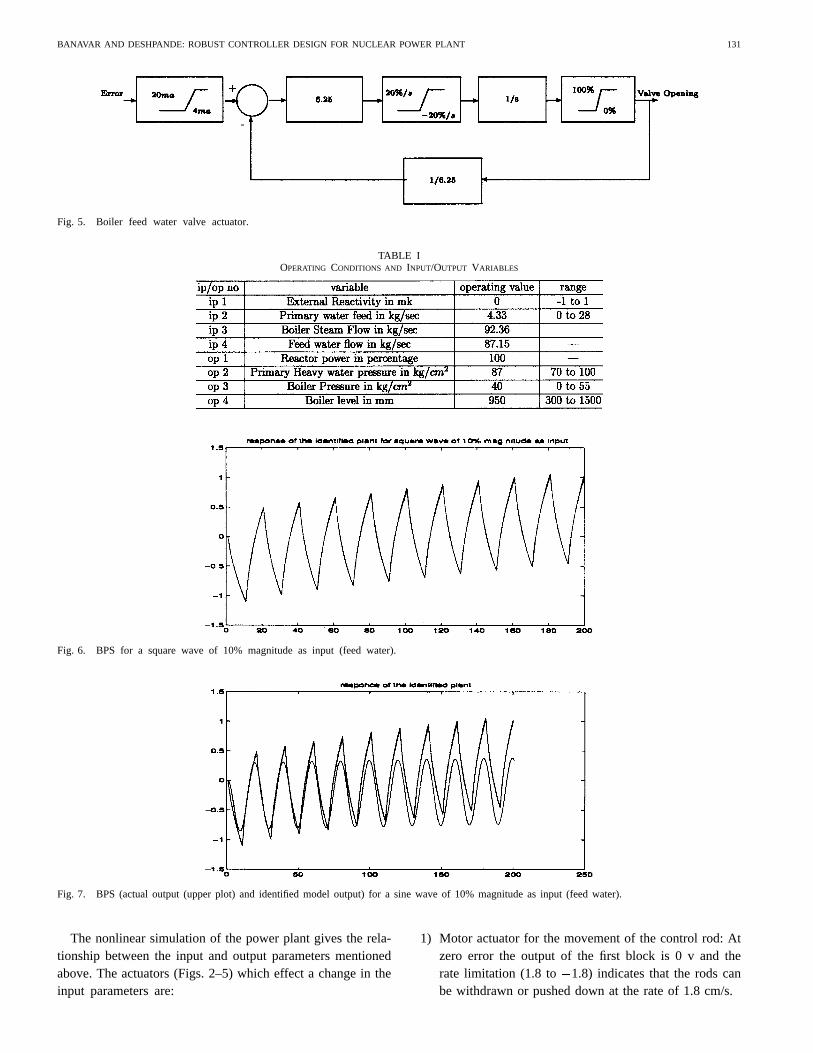
Fig. 5. Boiler feed water valve actuator.

TABLE IOPERATING CONDITIONS AND INPUT/OUTPUT VARIABLES

Fig. 6. BPS for a square wave of 10% magnitude as input (feed water).

Fig. 7. BPS (actual output (upper plot) and identified model output) for a sine wave of 10% magnitude as input (feed water).

The nonlinear simulation of the power plant gives the rela-tionship between the input and output parameters mentionedabove. The actuators (Figs. 2–5) which effect a change in theinput parameters are:

1) Motor actuator for the movement of the control rod: Atzero error the output of the first block is 0 v and therate limitation (1.8 to 1.8) indicates that the rods canbe withdrawn or pushed down at the rate of 1.8 cm/s.


Fig. 8. Reactor power (actual output (upper plot) and identified model output) for a square wave of 10% magnitude as input (BS flow).

Fig. 9. Reactor power (actual output (upper plot) and identified model output) for a sine wave of 10% magnitude as input (BS flow).

Fig. 10. Plant with actuator.

Fig. 11. Plant with precompensatorW:

2) Feed valve: At zero error, the output of the first block is4 mA. The rate limitation indicates a peak closing rateof 37%/s and an opening rate of172%/s.

3) Steam flow valve: At zero error, the output of the firstblock is 12 mA. The rate limitation indicates a peakclosing rate of 100%/s and an opening rate of300%/s.

4) Boiler feed valve: At zero error, the output of the firstblock is 16.8 mA. The rate limitation indicates a peakclosing rate of 20%/s and an opening rate of20%/s.

III. I DENTIFICATION OF THE PROCESS

The user-inputs to the executable program are as follows:

• the initial states and their derivatives;• the four inputs from the actuators, mentioned in Table I.

Operating values of the input-variables are provided toenable simulation of the plant at the operating condition.Table I lists the operating values of input and output variables.Since the objective of the controller is to attenuate disturbancesand adapt to small changes in the setpoint, linear models of themulti-input/multi-output (MIMO) system about the operatingcondition are extracted. As described in Section II, the powerplant has four inputs and four outputs. Since the system iscoupled, in all, 16 transfer functions are to be identified.Three of the outputs (reactor power, BPS, and BLVL) areunaffected by the primary heavy water flow. Hence thesetransfer functions are zero. For the basic theory and algorithmsused for identification, the interested reader is referred to [8]and [3].

A. Identification Procedure

Identification is carried out as follows.

1) To collect data for identification, a pseudorandom binarysignal (PRBS) is applied to the input. The magnitudeof the PRBS is within 10% of the total range forthat particular input variable at the operating point.While collecting data for a particular input/output (I/O)combination all the other inputs are set at their operatingvalues.

2) The data is fit to an auto-regressive-exogenous (ARX)model whose order is based on a loss function. Aquadratic loss function based on the prediction error is


TABLE IIIDENTIFIED REDUCED-ORDER TRANSFER FUNCTIONS

Fig. 12. Singular values of the plant.

evaluated. The model with the minimum value for theloss function is selected.

3) To avoid numerical instabilities and very high-ordercontrollers, it is essential to reduce the order of themodels which typically were of the 70th order. Aparticular analytic technique suitable in MIMOstablesystems is the balanced model order reduction which isbased on sensitivity analysis of the I/O properties. Inthis method, a balanced realization is first obtained by

Fig. 13. Singular values of the shaped plant.

using a transformation which uses the controllability andobservability Gramians and respectively, that areobtained from the Lyapunov equations [1]

(1)

where and denote the conventional state-spacemodel. The Hankel singular values (HSV) [7] of the


Fig. 14. The linear system.

Fig. 15. Coprime uncertainty description.

Fig. 16. Singular values of the controller.

system are given by

(2)

The HSV gives an indication of the contribution of aparticular state to the I/O behavior of the system. If aparticular HSV is very small, that particular state canbe neglected in the description of the system withoutappreciable change in the I/O properties [7]. The high-order models were reduced by balanced-order modelreduction.

4) The responses for inputs such as a square wave andsine wave are obtained. The output obtained by theidentified model and the one obtained by applying thesame input to the nonlinear simulation of the plant arecompared. The models with the lowest possible orderyielding satisfactory responses are selected.

Fig. 17. The closed-loop system.

5) The discrete model is converted to the continuous-timedomain by the TUSTIN approximation [6].

6) Since the control philosophy is optimization, itis desired that suitable uncertainty models be obtainedat the identification stage to quantify the bounds onuncertainty. Hence, after identification, the PRBS input(one used for identification) is applied to the model.The error in the output is calculated. Then the transferfunction between the error and the PRBS input is foundout by a similar procedure as explained above. Inparlance, this transfer function can be considered as an“additive uncertainty” block [4].

B. Transfer Functions and Related Graphs

The transfer functions obtained after the identificationprocess are presented in Table II. As mentioned earlier, thetransfer functions from the second input to outputs 1, 3, 4are zeros.

Responses for different inputs such as a square wave and asine wave are shown in Figs. 6–9.

IV. CONTROLLER DESIGN PROCEDURE

The controller is synthesized by using the normalized co-prime factorization approach. The reader is referred to [5],[9], [2], and [10] for a detailed treatment of -optimizationtheory.

The identification procedure yields the linear models be-tween perturbation inputs to the plant and perturbations inthe output of the plant around a nominal operating point,as shown in Fig. 10. The controller output is feed to theactuator. The block diagrams for the actuators are shown inFigs. 2–5.

A. Controller Design Procedure

1) The transfer functions initially identified are betweeninput and output as shown in Fig. 10. Including theactutator dynamics, the overall transfer function betweenthe actuator input and the plant output is computed.The order of the overall plant was found out to be70. The singular values of the system are shown inFig. 12. It should be mentioned at this stage that thenonlinearities in the actuator models are not incorporatedin the design as yet. Since all the nonlinearities thatappear in the problem are of the type that have a bounded

gain (i.e., finite energy input produces a finite energyoutput), they are treated as uncertainty blocks in the

paradigm with a bounded norm. As long as thecontroller designed provides guaranteed norm bounds


Fig. 18. Response of different outputs for a step in output power.

Fig. 19. Response of different inputs for a step in output power.

that are greater than the bounds of uncertainty due tothese nonlinearities, stability of the closed-loop systemis guaranteed. For more on this see [11].

2) To align the singular values in the frequency range ofinterest, a precompensator is designed (see Fig. 11).Specifications on the closed-loop system are indirectlyimposed by selecting the weighting function and ap-propriately adjusting the open-loop frequency response.Higher bandwidth of the shaped plant implies goodtracking ability of the closed-loop system. Similarly, lowgain in higher frequency implies better noise rejection.After designing the controller on the shaped plant, thesingular values of the sensitivity and complementarysensitivity transfer functions are checked. The controllershould be redesigned if the singular values of sensitivity

do not have the satisfactory shape. The singular val-ues of the sensitivity should have low gain in lowerfrequency region to get approximately zero steady-stateerrors. A point that should be noted while designingthe precompensator is that the shaped plant shouldhave approximately the same order of magnitude ofsteady state gains in all the channels. This is termed“plant normalization.” These are general guidelines fordesigning the precompensator and loopshaping.

Taking into consideration the above guidelines a prec-ompensator is designed to have an open-loop bandwidthof approximately 1 rad/s. The singular values are madeclose together at the gain crossover frequency. For thepurpose of simplicity, a diagonal matrix transfer function


Fig. 20. Response of different outputs for a step disturbance in PHTP.

Fig. 21. Response of different inputs for a step disturbance in PHTP.

of the form

where

is chosen as a precompensator. The singular values ofthe “shaped plant” to are shown in Fig. 13.

3) After loopshaping, a controller is designed using thenormalized coprime factorization approach. The coprimeuncertainty description has been found to be highlysuccessful in representing uncertainty in engineeringsystems [9]; hence we adopt this uncertainty model here.Fig. 15 shows the “generalized” plant (see [9]) for thecoprime uncertainty description of the plant. Hereand represent the normalized left coprime factors ofthe shapedplant. The resulting objective function to beminimized is

(3)


Fig. 22. Response of different outputs for a step disturbance in BPS.

Fig. 23. Response of different inputs for a step disturbance in BPS.

where

(4)

and denotes the maximum singular value. Thestate-space representation of the central controller givenby McFarlaneet al. [9] which ensures

(5)

is given by

(6)

where and are the solutions of the generalizedcontrol algebraic Riccati equation (GCARE) and thegeneralized filter algebraic Riccati equation (GFARE)respectively and

(7)

The synthesis procedure yields the controller ofFig. 14. The final controller is obtained by ap-pending the weights to The singular values to

of the final controller are shown in Fig. 16.Fig. 17 is a schematic of the closed-loop system with


Fig. 24. Response of different outputs for a step disturbance in BLVL.

Fig. 25. Response of different inputs for a step disturbance in BLVL.

the controller. The signal is the nominal value of theoutput at the operating condition. Similarly, is thenominal value of the input at the operating condition.Signals without a “” indicate the deviations from thenominal operating values in Fig. 17. The deviation ofthe output from its nominal operating value should bemaintained zero. Thus the setpoint signalin Fig. 17indicates the command signal for the deviation of theoutput from the nominal operating value, which is zeroif the system is expected to run at nominal conditions.

Figs. 18 and 19 show the command-following capa-bilities of the system for a unit step change in the power.Figs. 20–25 show the disturbance rejection characteris-tics for a unit output disturbance in the PHTP, BPS, andBLVL.

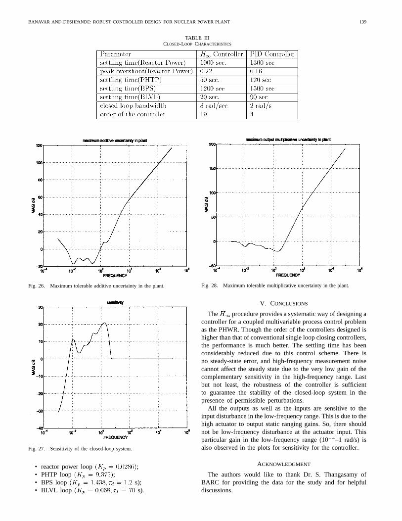
4) Robustness evaluation: The robustness of the controlleris confirmed by introducing an additive perturbation tothe plant dynamics and checking the stability of theclosed-loop system. Various responses for the perturbedplant are confirmed. Figs. 26–28 depict some of theserobustness properties. Further, as mentioned earlier, thevarious nonlinear elements such as saturation and ratelimitation in the actuators can be considered as additiveuncertainty blocks to the nominal plant. It is observedthat this uncertainty lies well below the maximum per-missible additive uncertainty shown in Fig. 26.

A few of the closed-loop characteristics are summarized inTable III. Steady-state error for all the channels is found tobe negligible. The gains of the existing proportional-integral-derivative (PID) controller in the plant are:


TABLE IIICLOSED-LOOP CHARACTERISTICS

Fig. 26. Maximum tolerable additive uncertainty in the plant.

Fig. 27. Sensitivity of the closed-loop system.

• reactor power loop ;• PHTP loop ;• BPS loop s);• BLVL loop s).

Fig. 28. Maximum tolerable multiplicative uncertainty in the plant.

V. CONCLUSIONS

The procedure provides a systematic way of designing acontroller for a coupled multivariable process control problemas the PHWR. Though the order of the controllers designed ishigher than that of conventional single loop closing controllers,the performance is much better. The settling time has beenconsiderably reduced due to this control scheme. There isno steady-state error, and high-frequency measurement noisecannot affect the steady state due to the very low gain of thecomplementary sensitivity in the high-frequency range. Lastbut not least, the robustness of the controller is sufficientto guarantee the stability of the closed-loop system in thepresence of permissible perturbations.

All the outputs as well as the inputs are sensitive to theinput disturbance in the low-frequency range. This is due to thehigh actuator to output static ranging gains. So, there shouldnot be low-frequency disturbance at the actuator input. Thisparticular gain in the low-frequency range (10–1 rad/s) isalso observed in the plots for sensitivity for the controller.

ACKNOWLEDGMENT

The authors would like to thank Dr. S. Thangasamy ofBARC for providing the data for the study and for helpfuldiscussions.


REFERENCES

[1] C. T. Chen, “Linear system theory and design,”HRW Series in Elec.Eng., 1984.

[2] J. C. Doyle, “Lecture notes in advances in multivariable control,” inProc. ONR/Honeywell Workshop, Minneapolis, MN, 1984.

[3] P. Eykhoff, System Identification: Parameter Estimation.London,U.K.: Wiley, 1974.

[4] B. Francis and J. Doyle, “Linear control theory with anH1 optimalitycriterion,” SIAM J. Contr. Opt., vol. 25, pp. 815–844, 1987.

[5] B. Francis, A Course inH1 Control Theory. Berlin, Germany:Springer Verlag, 1987.

[6] G. Franklin and J. D. Powell,Digital Control-Theory and Applications.New York: McGraw Hill, 1993.

[7] K. Glover, “All optimal Hankel norm approximations of linear multi-variable systems and theirL1 error bounds,”Int. J. Contr., vol. 39,pp. 1115–1193, 1984.

[8] L. Ljung, System Identification: Theory for Users. Englewood Cliffs,NJ: Prentice Hall, 1987.

[9] D. Mcfarlane and K. Glover,Robust Controller Design Using Normal-ized Coprime Factors. Berlin, Germany: Springer Verlag, 1990.

[10] D. C. Youla, H. A. Jabr, and J. Bongiorno, “Modern Wiener-Hopfdesign of optimal controllers—Part II,”IEEE Trans. Automat. Contr.,vol. AC-21, pp. 319–338, 1971.

[11] G. Zames, “On the input–output stability of time-varying nonlinearfeedback systems—Part 2: Conditions involving circles in the frequencyplane and sector nonlinearities,”IEEE Trans. Automat. Contr., vol.AC-11, pp. 465–476, July 1966.

robust controller design for a nuclear power plant using h∞ optimization

Documents