robust estimation of a linearized nonlinear regression...

Pertanika J. Sci. & Techno!. 6(1): 23 - 35 (1998)ISS : 0128-7680

© Universiti Putra Malaysia Press

Robust Estimation of a Linearized Nonlinear Regression Modelwith Heteroscedastic Errors:A Simulation Study

Habshah MidiMathematics Department

Faculty of Science and Environmental StudiesUniversiti Putra Malaysia

43400 UPM Serdang, Selangor, Malaysia

Received: 24 Disember 1996

ABSTRAK

Suatu kajian simulasi telah dijalankan untuk memeriksa keteguhan penganggarKuasadua Terkecil Biasa Dilinearkan (LOLS), penganggar Kuasadua TerkecilTeritlak Terjelma (TGLS) , penganggar Kuasadua Terkecil Berpemberat Terjelma(LRLS) dan penganggar Kuasadua Terkecil Berpemberat Terjelma Dilinearkan(TLRLS). Kaedah TLRLS adalah pengubahsuaian kaedah Kuasadua TerkecilBerpemberat (RLS) berasaskan kepada kaedah Median Kuasadua Terkecil(LMS). Kajian berangka menunjukkan bahawa penganggar LOLS, TGLS danLRLS tidak cukup teguh apabila peratusan titik terpencil di dalam datameningkat. Ini bermakna ketiga-tiga penganggar tersebut tidak mempunyaititik musnah yang tinggi. Keputusan kajian menunjukkan bahawa KaedahTLRLS mempunyai titik musnah yang tinggi berbanding dengan tiga kaedahyang lain.

ABSTRACT

A simulation study is used to examine the robustness of some estimators on alinearized nonlinear regression model with heteroscedastic errors, namely theLinearized Ordinary Least Squares (LOLS), Transformed Generalized LeastSquares (TGLS) , Linearized Reweighted Least Squares (LRLS) and TransformedLinearized Reweighted Least Squares (TLRLS). The latter is a modification ofReweighted Least Squares (RLS) based on Least Median of Squares (LMS).The empirical evidence shows that the first three estimators are not ufficientlyrobust when the percentage of outliers in the data increases. That is, they donot have a high breakdown point. On the other hand, the modified estimator(TLRLS) has a higher breakdown point than the other three estimators.

Keywords: breakdown point, outliers, generalized least squares,heteroscedasticity, least median of squares, linearized model, lognormal distribution, reweighted least squares

INTRODUCTION

The difficulty in computations involving a complex nonlinear structure can besolved by some transformation of the data so that it appears to follow a newmodel which is less complicated. A common type of transformation is tolinearize the nonlinear model by means of log transformation. However, it isnecessary to be aware of the consequences of using log transformation of a

Habshah Midi

nonlinear model with additive error terms. Such a transformation may alter theerror structure unless the error terms are multiplicative. While transformationmay solve the computational problem, it may produce another problem interms of violation of error structure. Thus, a clear advantage of linearization asfar as the properties of the estimators are concerned is not gained.

Consider the general nonlinear model with multiplicative error terms

Yi = f(X i , f3)E i (1.1 )

where [3T = ([31' [32 , , [3p) is the vector of parameters to be estimated. Theregressors Xi i = 1,2 , , are, in general, p dimensional vectors whose values areassumed known, and the errors Ej = 1,2, ... ,0 are i.i.d log-normal randomvariables, i.e. E - A(O, (J2Q) where A denotes a log-normal distribution and nis a n x n scale matrix.

In many applications, errors which are heteroscedastic, multiplicative andnot normally distributed may be encountered. Often the nature ofheteroscedasticitys not known. Heteroscedasticity is frequently modelled as afunction of covariates, mean response or other functional forms. By erroneuoslyassuming that the model has an error structure which is additive,_ normallydistributed, and n is an identity matrix, the least square estimator [3 is foundby minimizing the sum of squares

(1.2)

Using the Gauss-Newton Method (see Ratkowsky 1983), fi are obtained by

an iterative process. At the (k + l)th iteration, we have

where J (~) is the n x p Jacobian matrix, i.e.

df(X"

[3) df(X ,,[3) df(X I, [3)J[31 J[32 L J[3p

J([3') = M [3 [3*

df(X n , [3) df(XIl,[3) df(X n ,[3)

J[31 J[32 L J[3p

Starting with initial values for [3 at k = 0, the process continues untilconvergence, wh~ch occurs when l[3k+1 - [3(k>1 is smaller than some preselectedsmall quantity. [3 obtained from (1.3) is not asymptotically optimal when it

24 PertanikaJ. Sci. & Techno!. Vo!. 6 No.1, 1998

Robust Estimation of a Linearized Nonlinear Regression Model with Heteroscedastic Errors

violates the assumption of homoscedasticity. Moreover, equation (1.2) is notvalid when the error structure is really multiplicative instead of addtive innature. Consequently, a 'bad' estimator is obtained as a result of employing anincorrect formula on the erroneous a sumptions.

There are, however several nonlinear models which can be made linear bysome appropriate transformation. It should be noted, however, that thelinearization of the non-linear models may require the transformed error termsto be independent and normally distributed with mean °and constant variance,(j2.

Model (1.1) can be linearized by taking a natural logarithm that is,

Ln Y = Ln f(X,P) + Ln c

or it can be written as

Y = X'po + c'

where

Y = Ln Y, X'po = Ln f(X,P), c* = Ln c)

(1.4)

Ln c is normally distributed, i.e. Ln c. - N (O,(j2Q) since c. in model (1.1)follows a'log-normal distribution, i.e. c

j- A(O,(j2Q). The transfo~mationenables

the use of the standard regression method. It is very important to note thatwhen transformed models are employed, the estimators obtained by leastsquares have the least squares properties with respect to the transformedobservations, not the original ones, However, the ordinary Least Square Estimatorof the linearized model (LOLS) in (1.4),

(1.5)

is not an optimal estimator because Q is not an identity matrix. Let Q = ppTwhere P is an nxn diagonal matrix, i.e.

P =diag {l/~p(x)), 1/~p(x2)' L , l/~p(xn),}

The above problem of heteroscedasticity can be removed by means of asuitable transformation.

The transformed model is defined as

to give

PertanikaJ ci. & Techno!. Vo!. 6 No.1, 1998

(1.6)

25

Habshah Midi

where

This leads to

(1.7)

which is the best linear unbiased estimator with respect to the transformedmodel (1.4), and is called the generalized least square estimator on thetransformed variables (TGLS).

However, the drawback of the LOLS and the TGLS estimator is that theymay be affected by outliers, which are observations which significantly deviatingfrom the underlying model governing the bulk of the data. Hampel (1971)pointed out that even one single outlier can have an arbitrarily large effect onthe estimates. In this connection, he introduced the so-called breakdown point,c' as the smallest percentage of contaminated data that can cause an estimatorto take an arbitrarily large values. The robustness of each estimator depends onthe value of c'. An estimator becomes more robust as the value of c' increases.A better approach is to consider a robust method which is much less influencedby the outliers.

Several works on robust estimation have been proposed in the literature.Among them are Barrodale and Roberts (1973) and Armstrong and Kung(1978) who introduce L1-norm estimators. Huber (1973) proposed M-estimationand this was modified further by Krasker and Welsch (1982) who introducedbounded-influence regression estimator. one of these estimators achieves abreakdown point c' = 30% in the case of simple regression. Rousseeuw (1984)introduced the most robust regression estimator with the highest possiblebreakdown point, i.e. c' = 50%. This method is known as the Reweighted LeastSquares (RLS) based on the Least Median of Squares (LMS).

There have been numerous studies concerning the estimation of a linearmodel with heteroscedastic errors in the literature (Box and Hill 1974; Carrolland Ruppert 1982; Cohen et al1993). However, none of the studies has takeninto consideration the estimation of a high breakdown linear regression withheteroscedastic errors.

The focus of this study was to investigate the effect of outliers on theestimates of the linearized regression model when the errors are heteroscedastic.Consider a nonlinear model with multiplicative error terms, log-normallydistributed and heteroscedastic; i.e,

i.e. cj - ~(0,X2~. The mean and the variance of cj

are E(cj) =V(Cj) =e

2'; - e Xj respectively (Johnson and Kotz 1970).

(1.8)

and

26 PertanikaJ. Sci. & Techno!. Vo!. 6 No.1, 1998


By taking logarithms, model (1.8) can be written as a linear model:

Ln Yi = Ln ~o + Xi Ln ~l + Ln C j

where

(1.9)

The linearized model (1.9) is an additive model with hetercoscedasticerrors. It is very important to note that when heteroscedasticity prevails butother conditions of model (1.9) are satisfied, the estimators obtained byordinary least squares methods are still unbiased, but they are no longerminimum variance unbiased estimators. The variance of the error terms isproportional to x2

,V(t)=kx~, k~l. For simplicity, we take k = 1. The appropriatetransformations to obtain minimum variance unbiased estimators for model(1.9) are

Ln y x· 1y'X x

Model (1.9) then becomes

Ln Yi Ln /30 + In /31 + Ln ci(1.10)

Xi Xi Xi

A slight modification of the RLS method based on LMS is proposed. Thevalues of the variables X and yare then substituted with the values of thetransformed linearized variables l/x and L ny, respectively.

xThe modified method, known as the Transformed Linearized Reweighted

Least Squares (TLRLS) based on the LMS is performed by implementing theRLS method to the transformed linearized variables. We would expect themodified method to be more robust than the Linearized Ordinary LeastSquares (LOLS), the Transformed Generalized Least Squares (TGLS) and theLinearized Reweighted Least Squares (LRLS) procedures would maintain abreakdown point as high as 50%.

ROBUST REGRESSION ESTIMATOR

The Least Median of Squares (LMS) estimator (Rousseeuw 1984; Rousseeuwand Leroy 1987) is defined as the value that minimizes

where

median r.2I

T/3'r i = Yi - X , 1,2, .....n

(2.1)

PertanikaJ. Sci. & Techno!. Vo!. 6 No.1, 1998 27

Habshah Midi

for model (1.4).

This estimator is very robust with respect to outliers in y as well as outliersin x and also has the highest possible breakdown point, e' 50%.

The estimated variance, 0- is given by

(j' =

where

(2.2)

w ={li °

if h/sl ::; 2.5

otherwise(2.3)

s = 1.4826 {I + 5/(n-p)}~m~dri2I

In matrix notation, w; may be written as n x n diagonal matrix:

W = diag 1l,0,1,1, ... ,0, ..... 0,1}

t

(2.4)

the j'h outlier in the data set

Unfortunately, the LMS performs poorly (inefficient) when the errors areactually normally distributed. In order to impove the LMS estimator, Rousseeuwand Leroy (1987) introduced a method called Reweighted Least Squares (RLS)regression based on LMS, which is given by:

minimize L w.r.2• I I

f3

(2.5)

The weights Wi are determined from the LMS solutions (2.1), but with theestimated variance of (2.2) instead of (2.4). From (1.4), the LinearizedReweighted Least Square (LRLS) model can be written as: WY = WX' + We'.

Therefore, the LRLS estimator is given by

fi = (X'T WX') X'T WV' (2.6)

From (1.6), the Transformed Linearized Reweighted Least Squares (TLRLS)model then becomes

28 Perlanikaj. Sci. & Techno!. Vo!. 6 No. I, 1998

(2.7)


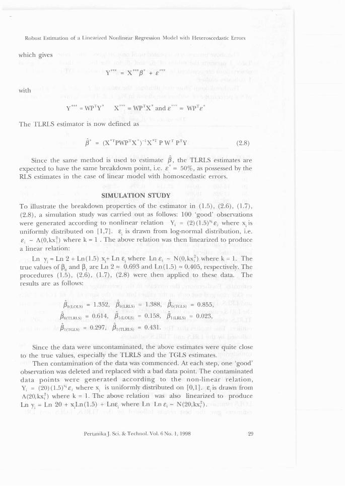
which gives

y*** X *** f3* + E ***

with

The TLRLS estimator is now defined as

(2.8)

Since the same method is used to estimate fi, the TLRLS estimates areexpected to have the same breakdown point, i.e. c' = 50%, as possessed by theRLS estimates in the case of linear model with homoscedastic errors.

SIMULATION STUDY

To illustrate the breakdown properties of the estimator in (1.5), (2.6), (1.7),(2.8), a simulation study was carried out as follows: 100 'good' observationswere generated according to nonlinear relation Yi = (2)(1.5)'i c; where Xi isuniformly distributed on [1,7]. ci is drawn from log-normal distribution, i.e.ci - A(O,kxi) where k = 1 . The above relation was then linearized to producea linear relation:

Ln y. = Ln 2 + Ln(1.5) x.+ Ln c. where Ln c; - N(0,kx2,.) where k = 1. The, "

true values of ~o and ~I are Ln 2 '" 0.693 and Ln(1.5) '" 0.405, respectively. Theprocedures (1.5), (2.6), (1.7), (2.8) were then applied to these data. Theresults are as follows:

fiO(LOLS) = 1.352, f30(LRLS) = 1.388, fiO(TGLS) = 0.855,

fiO(TLRLS) = 0.614, fil (LOLS) 0.158, fil (LRLS) = 0.023,

fil(TGLS) = 0.297, f31 (TLRLS) 0.431.

Since the data were uncontaminated, the above estimates were quite closeto the true values, especially the TLRLS and the TGLS estimates.

Then contamination of the data was commenced. At each step, one 'good'observation was deleted and replaced with a bad data point. The contaminateddata points were generated according to the non-linear relation,Yi = (20)(1.5)X; c; where Xi is uniformly distributed on [0,1]. c

iis drawn from

A(20, kxf) where k = 1. The above relation was also linearized to produceLn y. = Ln 20 + xLn(1.5) + Lnc. where Ln Ln c; - N(20,kxf).

, , I

PertanikaJ. Sci. & Technol. Vol. 6 No.1, 1998 29

Habshah Midi

The above process was repeated until only 50 'good' observations remained.Table 1 presents the values of iJo and iJl for the four methods, when goodobservations are replaced by certain percentages of outliers. OT noted in Table1 indicates outlier.

The breakdown plots that illustrate the values of iJo and iJl as a functionof the percentage of outliers are shown in Fig. 1, 2. These figures show that the

TABLE 1The values of iJ;and iJ~ for n = 100

/30 /31Method Method

%OT LOLS LRLS TGLS TLRLS LOLS LRLS TGLS TLRLS

0 1.352 1.388 0.855 0.614 0.158 0.023 0.297 0.43110 9.864 0.508 23.957 0.463 -1.515 0.517 -6.620 0.53220 14.569 0.506 23.114 0.398 -2.396 0.538 -5.555 0.56930 17.928 19.460 23.085 0.464 -3.032 -3.299 -4.717 0.60740 20.136 23.930 23.081 0.250 -3.558 -3.914 -3.960 0.65445 21.834 24.678 23.082 0.108 -3.695 -4.121 -3.713 0.71150 21.691 24.169 23.057 23.675 -3.879 -2.750 -3.300 -3.373

estimated values iJo and /31' which are based on the LOLS and TGLS wereimmediately affectd by the outliers. As can be expected, when there is nooutlier, the TGLS estimator performs better than the LOLS and the LRLSestimators. But as the percentage of outliers increases, the TGLS estimatesmove away from the true values drastically, followed by the LOLS and the LRLSestimates. Furthermore, the increase in the percentage of ou?iers from 0% upto 45% changed not only in the values but also the signs of /31 of TGLS, LOLSand LRLS, i.e. from positive to negative values. The results also point out thatthe LRLS estimates can tolerate slightly over 20% of outliers. The values of theTLRLS estimates seem to be consistent, before breaking down at 50% ofoutliers. This implies that The TGLS and the LOLS estimates break down first,followed by the LRLS and TLRLS estimates.

The breakdown properties of these estimates were investigated further byconsidering three samples of size 20, 50 and 100 observations. Simulationstudies were carried out in the manner described earlier. Tables 2, 3 and 4 showthe summary statistics, such as bias, standard error (SE) and root mean squareerror (RMSE) of the estimators. These results are very useful in assessing thebreakdown properties of the estimates.

These tables show that the TLRLS estimates are almost as good as theLOLS estimates in the normal error situation. As was to be expected, the TGLSestimates give the best results followed by the TLRLS, LOLS and LRLS

30 PertanikaJ. Sci. & Technol. Vol. 6 0.1,1998


60

LOLS

•LRLS

- - - .... - --TGLS

.......•......

TLRLS--,....-

50403020

•"".. ..•........ ...~ .. <.-t.:~.~.:.~~.::.::IIItIttIItItttI

10

5

30

25

0!S.,

20CO'-0en.,::> 15~"0~co 10E.::>~

Estimated Values of BetaO

Fig. 1. The breakdown plots of {3IJ

2

.. _~~~~~------~-----4------*--10 .....;,,;,,;,.;----------=-----------+--------1

..•.....

605040

TLRLS-->!---

TGLS

•30

----.. ---."-,t,;.,'

,,,,,~f"

.':.

20

...LOLS LRLS

• _u .... _u

.....

10

!S.,(2)co

'-0en.,::>

co (4)>"0.,iilE

(6)';:1

~

(8)0

Percentages of Outliers

Fig. 2. The breakdown plots of {3/

PertanikaJ. Sci. & Technol. Vol. 6 10 . I, 1998 31

Habshah Midi

TABLE 2Bias, SE, RMSE of {3~and f3, for n = 20

Outlier {3~ {3~% Method Bias SE RMSE Bias SE RMSE

LOLS 0.083 1.964 1.966 -0.014 0.615 0.615LRLS 0.159 2.136 2.142 -0.051 0.816 0.818

0 TGLS 0.100 1.367 1.370 -0.021 0.480 0.480TLRLS 0.109 2.104 2.106 -0.034 0.645 0.646

LOLS 9.338 2.143 9.580 -1.925 0.626 2.024LRLS 0.257 2.957 2.968 -0.041 0.886 0.881

10 TGLS 22.858 1.517 22.908 -6.894 1.020 6.969TLRLS 0.289 3.167 3.180 -0.051 0.801 0.801

LOLS 14.246 2.008 14.387 -2.965 0.637 3.032LRLS 2.140 6.550 6.891 -0.468 1.527 1.597

20 TGLS 23.644 1.003 23.665 -6.884 1.094 6.971TLRLS 0.635 4.180 4.227 -0.136 0.957 0.967

LOLS 17.339 1.811 17.434 -3.622 0.655 3.681LRLS 10.711 11.488 15.706 -2.320 2.656 3.526

30 TGLS 23.482 0.984 23.503 -6.358 1.198 6.470TLRLS 2.018 6.963 7.249 -0.416 1.509 1.565

LOLS 19.420 1.555 19.482 -4.078 0.698 4.137LRLS 22.265 5.816 23.012 -4.653 1.795 4.987

40 TGLS 23.283 0.926 23.301 -5.709 1.227 5.839TLRLS 6.828 10.965 12.917 -1.355 2.244 2.621

LOLS 20.959 1.330 21.001 -4.425 0.765 4.490LRLS 24.008 0.736 24.020 -3.693 1.390 3.946

50 TGLS 23.094 0.842 23.109 -4.961 1.262 5.119TLRLS 24.180 1.477 24.225 -4.551 1.556 4.809

estimates, when no contamination occurs in the model. The LOLS seems to bebetter than the LRLS estimator in this situation. It appears that the bias isalmost negligible and the variance makes up most of the MSE.

Nevertheless, as the percentage of outliers in the data becomes larger, theRMSE of the TGLS and the LOLS estimates increase significantly with thebiases making up most of the &\I1SE and the variances are rather small. TheTGLS estimates emerge to be conspicuously more efficient in the problem ofheteroscedasticity wi.th no contamination in the model. The LRLS estimatorcan be considered a good alternative for the case with slightly above 20%

outliers.On the other hand, the RMSE of the TLRLS estimates is consistently small

as the percentage of outliers becomes larger. Nonetheless, its values changed

32 PertanikaJ. Sci. & Technol. Vol. 6 No. I, )998


TABLE 3Bias, SE, RMSE of /3~and /3~ for n = 50

Outlier /3~ /3~% Method Bias SE RMSE Bias SE RMSE

LOLS 0.073 1.222 1.224 -0.008 0.386 0.386LRLS 0.126 1.375 1.381 -0.031 0.5430 0.543

0 TGLS 0.015 0.783 0.783 0.008 0.285 0.285TLRLS 0.032 0.978 0.978 0.005 0.339 0.339

LOLS 9.164 1.275 9.253 -1.887 0.382 1.926LRLS 0.057 1.666 1.667 0.005 0.559 0.559

10 TGLS 22.913 0.578 22.921 -6.896 0.653 6.927TLRLS 0.041 1.055 1.056 0.000 0.357 0.357

LOLS 14.076 1.215 14.129 -2.907 0.372 2.930LRLS 0.667 3.852 3.909 -0.127 0.905 0.914

20 TGLS 23.064 0.628 23.073 -6.480 0.766 6.626TLRLS 0.127 1.564 1.5669 -0.017 0.444 0.444

LOLS 17.130 1.106 17.166 -3.543 0.385 3.564LRLS 9.210 10.914 14.281 -1.892 2.321 2.995

30 TGLS 22.896 0.579 22.903 -5.828 0.817 5.885TLRLS 0.423 3.165 3.193 -0.076 0.706 0.710

LOLS 19.241 0.954 19.265 -3.989 0.389 4.008LRLS 23.713 2.050 23.801 -4.727 0.969 4.825

40 TGLS 22.738 0.457 22.743 -5.090 0.774 5.149TLRLS 2.416 7.278 7.669 -0.464 1.442 1.515

LOLS 20.805 0.835 20.821 -4.320 0.432 4.342LRLS 23.810 0.534 23.816 -3.210 1.103 3.395

50 TGLS 22.618 0.349 22.621 -4.307 0.738 4.370TLRLS 23.949 1.153 23.976 -4.212 1.210 4.383

dramatically at 50% of outliers. The results seem to be consistent in all 500 trialsand for each sample, size n = 20, 50, 100. The RMSE of the TLRLS estimatesare relatively smaller than the other three estimates. Summarizing the findingsfrom Tables 2, 3 and 4, it can be concluded that the TGLS and the LOLSestimates break down first and are then followed by the LRLS and TLRLSestimates. Thus, it can be concluded that the TLRLS estimates are the bestmethod for handling the problem of outliers in the linearized model when theerror terms are heteroscedastic.

PertanikaJ. Sci. & Techno\. Vo\. 6 No.1, 1998 33

Habshah Midi

TABLE 4Bias, SE, RMSE of ~~and fi~ for n = 100

Outlier fi~ fi~% Method Bias SE RMSE Bias SE RMSE

LOLS 0.027 0.822 0.823 -0.002 0.264 0.264LRLS 0.009 1.009 1.009 0.005 0.411 0.411

0 TGLS 0.009 0.506 0.506 0.005 0.193 1.193TLRLS 0.040 0.613 0.614 -0.004 0.227 0.227

LOLS 9.069 0.829 9.107 -1.863 0.265 1.882LRLS -0.026 0.949 0.949 0.021 0.373 0.374

10 TGLS 22.836 0.368 22.839 -6.838 0.432 6.852TLRLS -0.002 0.576 0.576 0.012 0.222 0.223

LOLS 13.971 0.794 13.994 -2.874 0.269 2.887LRLS 0.045 1.306 1.307 0.000 0.413 0.413

20 TGLS 22.7Ql 0.477 22.796 -6.265 0.512 6.286TLRLS 0.009 0.595 0.5959 0.010 0.230 0.230

LOLS 17.059 0.720 17.074 -3.508 0.273 3.518LRLS 7.639 10.244 12.779 -1.569 2.146 2.658

30 TGLS 22.632 0.359 22.634 -5.533 0.537 5.559TLRLS 0.026 0.624 0.624 0.010 0.239 0.239

LOLS 19.180 0.618 19.190 -3.941 0.281 3.951LRLS 23.787 0.612 23.795 -4.646 0.608 4.686

40 TGLS 22.551 0.275 22.553 -4.805 0.515 4.833TLRLS 0.405 3.179 3.205 -0.973 0.675 0.679

LOLS 20.720 0.530 20.727 -4.246 0.304 4.257LRLS 23.643 0.478 23.648 -2.853 1.014 3.028

50 TGLS 22.489 0.210 22.490 -4.055 0.083 4.084TLRLS 23.787 0.991 23.808 -4.071 1.157 4.232

CONCLUSION

The TGLS estimator of the linearized model is a better choice than the otherthree estimators in eliminating the problem of heteroscedasticity. Nevertheless,its performance was inferior to LOLS, LRLS and TLRLS estimators whencontamination occurred in the data. The LRLS estimator has a breakdownpoint slightly over 20% with the presence of outliers. It cannot provide a robustalternative to the TGLS and LOLS since it is not sufficiently robust when thepercentage of outliers increases. The simulation studies clearly shows that theTLRLS estimator is definitely the best because it is able to withstand a largeamount of outliers and has a highest breakdown point (up to 50% of outliers).Hence, it should provide a robust alternative to the well-known TGLS estimators.

34 PertanikaJ. Sci. & Technol. Vol. 6 No. I, 1998

Robust Estimation of a Linearized Tonlinear Regression Model with Heteroscedastic Errors

REFERENCES

AR.\1SfRO:-iG, R.D. and MT. KC:'\G. 1978. Least absolute values estimates for a simple linearregression problem. Applied Statistics 27: 363-366.

BARRODALE, 1 and F.D.K. ROBERTS. 1973. An improved algorithm for discrete L-l linearapproximation. Siam Journal of Numerical Analysis 10: 839-848.

Box, G.E.P. and WJ. HILL. 1974. Correcting inhomogeneity of variance with powertransformation weighting. Technometrics 16: 385-389.

CARROLL, RJ. and D. Ruppert. 1982. Robust estimation in heteroscedastic linear models.Ann. Stat. 10: 429-441.

COHEN, M., S.R. DALAL and J.W. TUKEY. 1993. Robust smoothly heterogeneous varianceregression. Appl. Statist. 42(2): 339-353.

HAMPEL, F.R. 1971. A general qualitative definition of robustness. Annals of MathematicalStatistics 42: 1887-1896.

HUBER, PJ. 1973. Robust estimation of a location parameter. Annals of MathematicalStatistics 35: 73-101. .

JOHNSON, .L. and S. KOTZ. 1970. DistrilJutions in Statistics-Continuous Univariate Df.strilJutions.Boston: Houghton Mifflin.

KRAsKER, W.S. and R.E. WELSCH. 1982. Efficient bounded-influence regression estimation.Journal of the American Statistical Association. 77: 595-605.

RATKOWSKY, DA. 1983. Non-Linear Regression Modelling. ew York: Marcel Dekker.

ROCSSEEUW, PJ. 1984. Least median of squares regression. Journal of the AmericanStatistical Association. 79: 871-879.

ROCSSEEUW, PJ. and A. LEROY. 1987. RolJust Regression and Outlier Detection. ew York:Wiley.

PertanikaJ. Sci. & Technol. Vol. 6 No.1, 1998 35

robust estimation of a linearized nonlinear regression...

Documents