robust parameterized component analysis

Robust Parameterized Component AnalysisTheory and Applications to 2D Facial Modeling

Fernando De la Torre1 and Michael J. Black2

1 Department of Communications and Signal Theory, La Salle School of Engineering,Universitat Ramon LLull, Barcelona 08022, Spain.

[email protected], http://www.salleURL.edu/˜ftorre/2 Department of Computer Science, Brown University, Box 1910, Providence, RI 02912, USA.

[email protected] http://www.cs.brown.edu/˜black/

Abstract. Principal Component Analysis (PCA) has been successfully applied toconstruct linear models of shape, graylevel, and motion. In particular, PCA hasbeen widely used to model the variation in the appearance of people’s faces. Weextend previous work on facial modeling for tracking faces in video sequencesas they undergo significant changes due to facial expressions. Here we developperson-specific facial appearance models (PSFAM), which use modular PCA tomodel complex intra-person appearance changes. Such models require aligned vi-sual training data; in previous work, this has involved a time consuming and error-prone hand alignment and cropping process. Instead, we introduce parameterizedcomponent analysis to learn a subspace that is invariant to affine (or higher order)geometric transformations. The automatic learning of a PSFAM given a trainingimage sequence is posed as a continuous optimization problem and is solved witha mixture of stochastic and deterministic techniques achieving sub-pixel accuracy.We illustrate the use of the 2D PSFAM model with several applications includingvideo-conferencing, realistic avatar animation and eye tracking.

1 Introduction

Many computer vision researchers have used Principal Component Analysis (PCA) toparameterize appearance, shape or motion [3,10,23,30]. However, one major drawbackof this traditional technique is that it needs normalized samples in the training data. In thecase of computer vision applications, the result is that the samples have to be aligned orgeometrically normalized (we assume that other normalizations, e.g. photometric, havealready been done). Previous methods for constructing appearance or shape models [10,16,17,23,30,31] have cropped the region of interest by hand, or have used a hand-labeledpre-defined feature points to apply the translation, scaling and rotation that brought eachimage into alignment with a prototype. These manual approaches are likely to introduceerrors into the model due to inaccuracies which arise from labeling the points by hand.In addition, manual cropping is a tedious, unpleasant, and time consuming task. Thispaper automates this process with a general framework for learning low dimensionallinear subspaces while automatically solving for the alignment of the input data withsub-pixel accuracy.

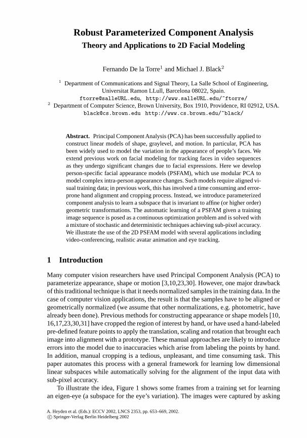
To illustrate the idea, Figure 1 shows some frames from a training set for learningan eigen-eye (a subspace for the eye’s variation). The images were captured by asking

A. Heyden et al. (Eds.): ECCV 2002, LNCS 2353, pp. 653–669, 2002.c© Springer-Verlag Berlin Heidelberg 2002

654 F. De la Torre and M.J. Black

Fig. 1. Some frames of the original image sequence.

a:

b:

c:

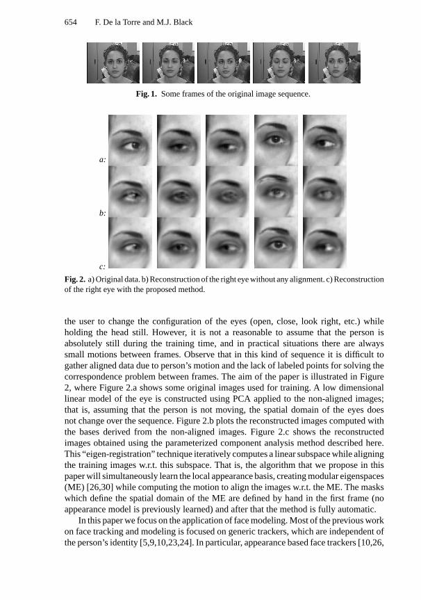
Fig. 2. a) Original data. b) Reconstruction of the right eye without any alignment. c) Reconstructionof the right eye with the proposed method.

the user to change the configuration of the eyes (open, close, look right, etc.) whileholding the head still. However, it is not a reasonable to assume that the person isabsolutely still during the training time, and in practical situations there are alwayssmall motions between frames. Observe that in this kind of sequence it is difficult togather aligned data due to person’s motion and the lack of labeled points for solving thecorrespondence problem between frames. The aim of the paper is illustrated in Figure2, where Figure 2.a shows some original images used for training. A low dimensionallinear model of the eye is constructed using PCA applied to the non-aligned images;that is, assuming that the person is not moving, the spatial domain of the eyes doesnot change over the sequence. Figure 2.b plots the reconstructed images computed withthe bases derived from the non-aligned images. Figure 2.c shows the reconstructedimages obtained using the parameterized component analysis method described here.This “eigen-registration” technique iteratively computes a linear subspace while aligningthe training images w.r.t. this subspace. That is, the algorithm that we propose in thispaper will simultaneously learn the local appearance basis, creating modular eigenspaces(ME) [26,30] while computing the motion to align the images w.r.t. the ME. The maskswhich define the spatial domain of the ME are defined by hand in the first frame (noappearance model is previously learned) and after that the method is fully automatic.

In this paper we focus on the application of face modeling. Most of the previous workon face tracking and modeling is focused on generic trackers, which are independent ofthe person’s identity [5,9,10,23,24]. In particular, appearance based face trackers [10,26,

Robust Parameterized Component Analysis 655

34] make use of PCA in order to construct a linear model of the face’s subspace (variationacross people) rather than the intra-person variations due to changes in expression.When working with person-specific models [15,17,20,23], PCA will model the complexintra-person appearance changes due mostly to variations of expression (eyes’ blinking,wrinkles in the mouth area, appearance of the teeth, etc.) rather than modeling theappearance changes due to identity. Although PSFAM are just valid for one person, theyremain useful in many vision related applications such as vision-based human computerinteraction (VBHCI), speech driven animation (to animate faces from audio), facialanimation in general, video-conferencing, face verification, etc, which usually involvea particular user. In related but different work, Edwards et al. [19,20] have proposeda method for approximately isolating the sources of image variation such as identity,pose, lighting, etc [19] by using linear discriminant analysis. Edwards et al. [20] usethis factorized basis to update some characteristics to personalize a model. In this paper,we will apply Robust Parameterized Component Analysis to learn a PSFAM and willillustrate the method with applications involving facial modeling. Preliminary results ofthis paper were presented in [12].

2 Previous Work

This paper is related to previous work on subspace learning methods and PCA. It isbeyond the scope of the paper to review all possible applications of PCA, therefore wejust briefly describe the theory and point to related work for further information.

2.1 Subspace Learning

LetD = [d1 d2 ... dN ] = [d1 d2 ... dd]T be a matrixD ∈ �d×N 1, where each columndi is a data sample (or image),N is the number of training images, andd is the numberof pixels (variables) in each image. If the effective rank ofD is much less thand, we canapproximate the column space ofD with k << d principal components. Let the firstkprincipal components ofD beB = [b1, ...,bk] ∈ �d×k. The columns ofB span thesubspace of maximum variation of the dataD.

Although a closed form solution for computing the principal components (B) canbe achieved by computing thek largest eigenvectors of the covariance matrixDDT

[18], here it is useful to exploit work that formulates PCA as the minimization of anenergy function [14,18]. Related formulations have been studied in various communities

1 Bold capital letters denote a matrixD, bold lower-case letters a column vectord. dj representsthe j-th column of the matrixD anddj is a column vector representing thej-th row of thematrix D. dij denotes the scalar in rowi and columnj of the matrixD and the scalari-thelement of a column vectordj . All non-bold letters represent scalar variables.dji is thei-thscalar element of the vectordj .diag is an operator that transforms a vector to a diagonal matrix,or a matrix into a column vector by taking each of its diagonal components.tr(D) is the traceoperator for a square matrixD ∈ �d×d, that is,

∑di=1 dii. ||d||22 denotes theL2 norm of the

vectord, that isdT d. ||d||2W denotes the weightedL2 norm of the vectord, that isdT Wd,and||D||2F is the Frobenius norm of a matrix,tr(DT D) = tr(DDT ). D1 ◦ D2 denotes theHadamard (point wise) product between two matrices of equal dimension.


(see [14]): machine learning, statistics, neural networks and computer vision. In spirit,all these approaches essentially minimize the following energy function (although withdifferent noise models, deterministic or Bayesian frameworks, or different metrics):

Epca(B,C) = ||D − BC||2F =N∑

i=1

||di − Bci||22 =N∑

t=1

d∑p=1

(dpt −k∑

j=1

bpjcjt)2 (1)

whereC = [c1 c2 · · · cn] and eachci is a vector of coefficients used to reconstruct thedata vectordi. It is interesting to note that the three equivalent previous equations cangive different insights into the subspace learning technique. The first matrix formulationclearly poses PCA as a simple factorization ofD intoB andC. The problem of subspacelearning translates to a bilinear estimation process of matricesB andC. The secondequivalence shows more explicitly how each data sampledi is reconstructed with acoefficientci and a common basisB. Finally the last equation expresses the subspaceconstraint at a pixel level. Many methods exist for minimizing (1) (Alternated LeastSquares (ALS), Expectation-Maximization (EM), etc.), but in the case of PCA, share thesame basic philosophy. These algorithms alternate between solving for the coefficientsC with the basesB fixed and then solving for the basesB with C fixed. Typically, bothupdates are computed by solving a linear system of equations.

2.2 Adding Motion into the Subspace Formulation

Principal component analysis has been widely applied to the construction of facial mod-els using linear subspaces [34]. During recognition or tracking it is common to automat-ically align the input images with the eigenspace using some optimization technique [4,10,34]. In contrast, little work has addressed problems posed by facial misalignment atthe learning stage. Mis-registration introduces significant non-linearities in the manifoldof faces and can reduce the accuracy of tracking and recognition algorithms.While previ-ous approaches have dealt with these issues as a separate, off-line registration processes(often manual), here it is integrated into the learning procedure.

Recently there has been an interest in the simultaneous computation (although theexisting algorithms compute it iteratively) of appearance bases and motion. This problemis is a classical chicken-and-egg problem (like motion segmentation). Once the pixelcorrespondence between the images in the training data is solved, learning the appearancemodel is straightforward, and if the appearance is known, solving for the correspondenceis easy. De la Torre et al. [15] proposed a method for face tracking which recovers affineparameters using subspace methods. This method dynamically updates the eigenspaceby utilizing the most recent history. The updating algorithm estimates the parametrictransformation, which aligns the actual image w.r.t. the eigenspace and recalculates alocal eigenspace. Because the new images usually contain information not available inthe eigenspace, the motion parameters are calculated in a robust manner. However, themethod assumes that an initial eigenspace is learned from a training set aligned by hand.Schweitzer [33] has proposed a deterministic method which registers the images withrespect to their eigenfeatures, applying it to theflower garden sequence for indexingpurposes. However, the assumption of affine or quadratic motion models is only valid


when the scene is planar. The extension to the general case of arbitrary 3D scenes andcamera motions remains unclear. As Schweitzer notices [33] the algorithm is likelyto get stuck in local minima, since it comes from a linearization and uses gradientdescent methods. On the other hand, Rao [32] has proposed a neural-network whichcan learn a translation-invariant code for natural images. Although he suggests updatingthe appearance basis, the experiments show only translation-invariant recognition, asproposed by Black and Jepson [4].

Frey and Jojic [21] took a different approach and they introduce an ExpectationMaximization (EM) algorithm for factor analysis (similar to PCA) that is invariant togeometric transformations. While their work represents a significant and pioneeringcontribution, the proposed method can be problematic because it discretizes the space ofspatial transformations and the computational cost grows exponentially with the numberof possible transformations. Our work attempts to solve a similar problem but with acontinuous optimization framework that is more appropriate for common parameterizedtransformations of the data (e.g. affine).

In a different direction, there has been intensive research on automatically or semi-automatically aligning facial shape models using extracted landmarks. See [11] fora good review of automatic 2D and 3D landmark placement. In contrast to previousautomatic landmark methods, we use parameterized matching with a low dimensionalmodel (e.g. affine) and generalize the matching by solving for both the subspace of theappearance variation and the alignment of the training data with the subspace.

In this paper, unlike previous methods we use stochastic and multi-resolution tech-niques to avoid local minima in the minimization process. Also, we extend previousapproaches to multiple regions within a robust (to outliers) and continuous optimizationframework. We apply the method to learn 2D modular PSFAMs and several potentialapplications of PSFAMs are proposed.

3 Generative Face Models: Motivation

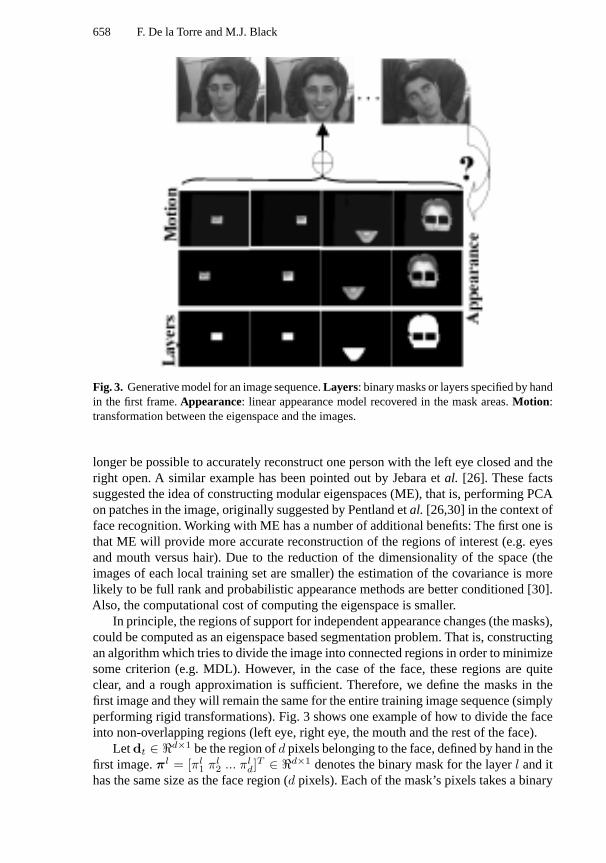
Our eigen-registration algorithm will be introduced with examples from face modeling.In this section we describe one possible generative model for dynamic faces. Similar tothe previous work of Black and Jepson [4], Black etal. [3] and Cootes etal. [10], thegenerative model that we propose for image formation takes into account motion andappearance, but in our case we also exploit predefined masks and learn the appearancebases. Figure 3 shows some frames of a training set for learning a 2D PSFAM. Given thistraining data as an input, the algorithm that we propose in this paper is able to factorizethe training data into appearance and motion of some predefined regions.

3.1 Modular Eigenspaces

The eyes and the mouth, while weakly correlated, can perform independent graylevelchanges (over a long sequence), so they should be represented in different eigenspacesin order to facilitate interpretation, to allow a more flexible model and to generate amore compact representation. Consider, for instance, a training set of people with botheyes open or both eyes closed. If we consider the face as a unique region, it would no


Fig. 3. Generative model for an image sequence.Layers: binary masks or layers specified by handin the first frame.Appearance: linear appearance model recovered in the mask areas.Motion:transformation between the eigenspace and the images.

longer be possible to accurately reconstruct one person with the left eye closed and theright open. A similar example has been pointed out by Jebara etal. [26]. These factssuggested the idea of constructing modular eigenspaces (ME), that is, performing PCAon patches in the image, originally suggested by Pentland etal. [26,30] in the context offace recognition. Working with ME has a number of additional benefits: The first one isthat ME will provide more accurate reconstruction of the regions of interest (e.g. eyesand mouth versus hair). Due to the reduction of the dimensionality of the space (theimages of each local training set are smaller) the estimation of the covariance is morelikely to be full rank and probabilistic appearance methods are better conditioned [30].Also, the computational cost of computing the eigenspace is smaller.

In principle, the regions of support for independent appearance changes (the masks),could be computed as an eigenspace based segmentation problem. That is, constructingan algorithm which tries to divide the image into connected regions in order to minimizesome criterion (e.g. MDL). However, in the case of the face, these regions are quiteclear, and a rough approximation is sufficient. Therefore, we define the masks in thefirst image and they will remain the same for the entire training image sequence (simplyperforming rigid transformations). Fig. 3 shows one example of how to divide the faceinto non-overlapping regions (left eye, right eye, the mouth and the rest of the face).

Letdt ∈ �d×1 be the region ofd pixels belonging to the face, defined by hand in thefirst image.πl = [πl

1 πl2 ... πl

d]T ∈ �d×1 denotes the binary mask for the layerl and it

has the same size as the face region (d pixels). Each of the mask’s pixels takes a binary


value,πlp ∈ {0, 1} and there is no overlap between masks, that is,

∑Ll=1 π

lp = 1 ∀ p .

πl will containdl pixels with value1, which define the spatial domain of the maskl (seeFig. 3) and

∑Ll=1 dl = d.

Each of these masks will have an associated eigenspace. The graylevel of the patch,or layerl, will be reconstructed by a linear combination of an appearance basisBl:

dt =

d1t...

dLt

=

B1c1t

...BLcL

t

=

L∑i=1

(πl ◦ Blclt) (2)

wheredlt ∈ �dl×1 is the patch of the layerl andcl

t are the appearance coefficients ofthe layerl at timet. Bl = [bl

1 bl2 ... b

lkl

] ∈ �dl×kl are thekl appearance bases for thel

layer.Bl ∈ �d×kl will be equal toBl for all pixels whereπlp = 1 (i.e. belonging to the

lth mask) and otherwise can take an arbitrary value.

3.2 Motion

If the face to be tracked can be considered to be far away from the camera, it canbe approximated by a plane [5]. The motion of planar surfaces, under orthographic orperspective projection, can be recovered with a parametric model of6 or 8 parameters.The rigid motion of the face will be parameterized by an affine model:

f1(xp,alt) =

[al1t

al4t

]+

[al2t al

3t

al5t al

6t

] [xp − xl

c

yp − ylc

](3)

wherealt = [al

1t al2t . . . al

6t]T denotes the vector of motion parameters of the maskl at

time t, xp = [xp yp]T are the Cartesian coordinates of the image at thepth pixel andxl

c = [xlc yl

c]T is the center of thel layer. Throughout the paper, we will assume that

the rigid motion of all the modular eigenspaces (w.r.t. the center of the face) is the same.That is,a1

t = a2t . . . = aL

t .Once the appearance and motion models have been defined, the graylevel of each

pixel of the imagedt is explained as a superposition of a layer-subspace plus a warping,see Fig. (3); that is,dt =

∑Ll=1

(πl ◦ Blcl

t

)(f1(x,al

t)), wherex = [x1 x2 · · · xd]T .

The notation(πl◦Blcl

t

)(f1(x,al

t))

means that the reconstructed image within the mask,(πl ◦ Blcl

t

), is warped (or indexed) by the parameterized transformationf1(x,al

t). Ob-serve that this image model is essentially the same as previous appearance representations[4,10,16] but with the addition of modular eigenspaces.

4 Learning the Model Parameters

Once the model has been established, in order to automatically learn the PSFAM, it is nec-essary to learn the model parameters. In this section we describe the learning procedure;that is, given an observed image sequence(D ∈ �d×N ) (N is the number of images) andL masks in the first image (π = {π1, . . . ,πL}), finding the parametersB, C, A andσ,


which best reconstruct the sequence. WhereA = {A1, A2, ... ,AL} is the set of motionparameters of all the layers in all the image frames.Ai = [ai

1 ai2 · · · ai

N ] is the ma-trix which contains the motion parameters for each image in theith layer. Analogously,C = {C1, C2, ... ,CL} whereCi = [ci

1 ci2 · · · ci

N ] andB = {B1, B2, ... ,BL}.At this point, learning the model parameters can be posed as a minimization problem.

In this case the residual will be the difference between the image at timet and thereconstruction with the model. In order to take into account outlying data, we introducea robust objective function, minimizingErereg(B, C,A;σ):

Erereg =∑N

t=1∑d

p=1 ρ

(dpt − ∑L

l=1

(πl

p

∑kj=1 b

lpjc

ljt

)(f1(xp,al

t)), σp

)(4)

whereblpj is thepth pixel of thejth basis ofBl for the layerl. Observe that the pixel

residual isfiltered by the Geman-McClure robust error function [22] given byρ(x, σp) =x2

x2+σ2p, in order to reduce the influence of outlying data.σp is a parameter that controls

the convexity of the robust function and is used for the deterministic annealing in aGraduated Non-Convexity algorithm [4,7] (we do not minimizeErereg overσp). Benefitsof the robust formulation in the subspace related problems are explained elsewhere [14].Observe that the previous Eq. (4) is similar toEigentracking [4] but is applied in imagepatches (masks). It is also similar to AAM [10] orFlexible Eigentracking [16] withoutshape constraints. However, in contrast to these approaches [4,10,16], inErereg theappearance basesB are now treated as parameters to be estimated.

4.1 Stochastic State Initialization

The error functionErereg, Eq. (4), is non-convex and, without a good starting point,gradient descent methods are likely to get trapped in local minima. When computingthe motion parameters, as in the case of optical flow, a coarse-to-fine strategy [4,11] canhelp to avoid local minima. Although a coarse-to-fine strategy is helpful, this techniqueis insufficient in our case, since in real image sequences the size of the face can be smallin comparison to the number of pixels in the background, and large motions can beperformed (e.g. in the sequences that we tried, the face can move more than 20 pixelsfrom frame to frame). In order to cope with such real conditions, we explore the useof stochastic methods such as Simulated Annealing (SA) [2], Genetic Algorithms (GA)[27,29] orCondensation (particle filtering) [6,17] for motion estimation. Although thetechniques are very similar computationally speaking, here we make use of GA [29]within a coarse-to-fine strategy.

Given the first image of the sequence, we manually initialize the layers or masks atthe highest resolution level and assign the graylevel to the first bases for each layerB ={b1

1, . . . ,bL1 }. Afterwards, we take the subset of them frames closest in time (typically

m=15), and use a GA for a first estimation of the motion parameters which minimizeEq. (4) (the least squares version). Given the genetic estimation of these parameters, werecompute the basesB which preserve60% of the energy. This initialization procedureis repeated until all the frames in the image sequence are initialized. The procedure issummarized as:


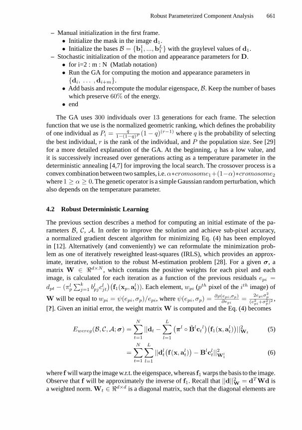
– Manual initialization in the first frame.• Initialize the mask in the imaged1.• Initialize the basesB = {b1

1, ...,bL1 } with the graylevel values ofd1.

– Stochastic initialization of the motion and appearance parameters forD.• for i=2 : m : N (Matlab notation)• Run the GA for computing the motion and appearance parameters in

{di, . . . ,di+m}.• Add basis and recompute the modular eigenspace,B. Keep the number of bases

which preserve60% of the energy.• end

The GA uses300 individuals over13 generations for each frame. The selectionfunction that we use is the normalized geometric ranking, which defines the probabilityof one individual asPi = q

1−(1−q)P (1 − q)(r−1) whereq is the probability of selectingthe best individual,r is the rank of the individual, andP the population size. See [29]for a more detailed explanation of the GA. At the beginning,q has a low value, andit is successively increased over generations acting as a temperature parameter in thedeterministic annealing [4,7] for improving the local search. The crossover process is aconvex combination between two samples, i.e.α∗cromosome1+(1−α)∗cromosome2where1 ≥ α ≥ 0. The genetic operator is a simple Gaussian random perturbation, whichalso depends on the temperature parameter.

4.2 Robust Deterministic Learning

The previous section describes a method for computing an initial estimate of the pa-rametersB, C, A. In order to improve the solution and achieve sub-pixel accuracy,a normalized gradient descent algorithm for minimizing Eq. (4) has been employedin [12]. Alternatively (and conveniently) we can reformulate the minimization prob-lem as one of iteratively reweighted least-squares (IRLS), which provides an approx-imate, iterative, solution to the robust M-estimation problem [28]. For a givenσ, amatrix W ∈ �d×N , which contains the positive weights for each pixel and eachimage, is calculated for each iteration as a function of the previous residualsepi =dpt − (πl

p

∑kj=1 b

lpjc

ljt

)(f1(xp,al

t)). Each element,wpi (pth pixel of theith image) of

W will be equal towpi = ψ(epi, σp)/epi, whereψ(epi, σp) = ∂ρ(epi,σp)∂epi

= 2epiσ2p

(e2pi+σ2

p)2 ,

[?]. Given an initial error, the weight matrixW is computed and the Eq. (4) becomes

Ewereg(B, C,A;σ) =N∑

t=1

||dt −L∑

l=1

(πl ◦ Blct

l)(

f1(x,alt)

)||2Wt(5)

=N∑

t=1

L∑l=1

||dlt

(f(x,al

t)) − Blcl

t||2Wlt

(6)

wheref will warp the image w.r.t. the eigenspace, whereasf1 warps the basis to the image.Observe thatf will be approximately the inverse off1. Recall that||d||2W = dT Wd isa weighted norm.Wt ∈ �d×d is a diagonal matrix, such that the diagonal elements are


the tth column ofW. Wlt ∈ �dl×dl is diagonal matrix, where the diagonal is created

by the elements of thet column ofW which belong to thelth layer. Observe that ifWis a matrix with all ones we have the least-squares solution.

Eq. (6) provides the formulation for robusteigen-registration or robust parameterizedcomponent analysis. Minimizing (6) with respect to the parameters gives a subspacethat is invariant to the allowed geometric transformations and robust to outliers on apixel level. Clearly, finding the minimum is a challenge and the process for doing so isdescribed below.

Notice that, if the motion parameters are known, computing the basis (B) and thecoefficients (C) translates into a weighted bilinear problem. In order to compute theupdates of the bases and coefficients in closed form in the simplest way, we use thefollowing observation:

Ewereg(B, C,A;σ) =N∑

t=1

L∑l=1

||(dlw)t − Blcl

t||2Wlt

(7)

=dl∑

p=1

L∑l=1

||(dlw)p − (Cl)T (bl)p||2(Wl)p (8)

where(dlw)t is the warped imagedl

t

(f(x,at)

)and it is thetth column of the matrix

Dw (just thedl elements corresponding to thel layer). Recall that(dlw)p is a column

vector which corresponds to thepth row of the matrixDw and that(Wl)p is a diagonalmatrix which contains thepth row of the matrixW of the layerl.

Minimizing Eq. (6) is a non-linear optimization problem w.r.t. the motion parameters.Following previous work on motion estimation [4,24], we linearize the variation ofthe function, using a1st order Taylor series approximation. Without loss of generality,rather than linearizing the transformation which warps the eigenspace towards the imagef1(x,at), we linearize the transformation which aligns the incoming image w.r.t. theeigenspacef(x,at) (see Eq. 6). Expanding,dl

t(f(x,al0t + ∆al

t)) in the Taylor seriesabout the initial estimation of the motion parametersal0

t (given by the GA):

dlt(f(x,a

l0t + ∆al

t)) = dlt(f(x,a

l0t )) + Jl

t∆alt + h.o.t. (9)

whereJlt is the Jacobian at timet of the lth layer andh.o.t. denotes the higher order

terms. Observe that after the linearization the functionEwereg, Eq. (6), is convex ineach of the parameters. For instance,∆at can be computed in closed form solving alinear system of Equations:

((J1

t )T W1

t J1t

)((J2

t )T W2

t J2t

)..(

(JLt )T WL

t JLt

)

[∆at

]=

(J1t )

T W1t (dt(f(x,a0

t )) − B1c1t )

(J2t )

T W2t (dt(f(x,a0

t )) − B2c2t )

.

.

(J1t )

T WLt (dt(f(x,a0

t )) − BLcLt )

where recall thatWlt is a matrix containing the weights for the layerl at timet. In this

case, we have assumed that∆alt = ∆at ∀ l because the modular eigenspaces share the

motion parameters, therefore we drop the superscriptl in the motion parameters.


However,Ewereg is no longer convex as a joint function of these variables. In orderto learn the parameters, we break the estimation problem into two sub-problems. Wealternate between estimatingC andA with a Gauss-Newton scheme [4] and learning thebasisB and scale parametersσ until convergence, see [14] for more detailed information.Each of the updates forC,A andB are done in closed form. This multi-linear fittingalgorithm monotonically reduces the cost function, although it is not guaranteed toconverge to the global minimum. We also use a coarse-to-fine strategy [4,11] to copewith large motions and to improve the efficiency of the algorithm. Towards that end,a Gaussian image pyramid is constructed. Each level of the pyramid is constructed bytaking the image at the previous resolution level, convolving it with a Gaussian filter andsub-sampling. Details of the learning method are given below.

– For each image resolution level until convergence ofC,A andB• Until convergence ofC,A

∗ Until convergence ofA, rewarpD toDw and update the motion parametersfor each layer by computing:(al

t) = (alt) + ∆at ∀ l = 1 . . . L

∗ Update the appearance coefficients for each layer and each image((Bl)T Wl

tBl)cl

t = (Bl)T Wltdt(f(x,al

t)) ∀ l = 1 . . . L, ∀ t = 1 . . . N• UpdateB preserving85% of the energy, solving:

(Cl(Wl)p(Cl)T )(bl)p = Cl(Wl)p(dlw)p ∀ l = 1 . . . L, ∀ p = 1 . . . dl

• Recompute the error, weights (W) and the scale statisticsσ [14].

– Propagate the motion parameters to the next resolution level [4,11] (the translationparameters are multiplied by a factor 2). Once the motion parameters are propagatedthe bases are recomputed.

5 Experiments and Applications

5.1 Automatic Learning of Eigeneyes

Eyes are one of the key elements inVision Based Human Computer Interaction (VBHCI).In this experiment, we automatically learn a person-specific “eigeneye” without anymanual cropping, except in the first image. We assume that during the training processthe person is not moving far away (around 5-8 pixels) from the first frame.

Recall that Fig. 1 illustrates the eigen-registration method and shows a few imagesfrom a training set. In the first frame, we manually select the mask for the eyes, face,and background (in Fig. 6 the regions are represented). In this case, because we areassuming a small motion, the GA has not been applied for initializing the algorithm,and we minimize Eq. (6) with the robust deterministic learning method proposed, witha coarse-to-fine strategy (2 levels) over the entire training set (around 300 frames). Wehave presupposed that the data had few outliers, so we giveσ a high value.

In Fig. 2 the reconstruction of some right eye training images are shown. Fig. 2.ashows the original images, Fig. 2.b plots the reconstructed images with non-alignedbasis (assuming that the person is not moving, each layer does not change over thesequence). Fig. 2.c represents the reconstructed images after minimizing Eq. (6). As


0 50 100 150 200 250 3000.01

0.02

0.03

0.04

0.05

0.06

0.07

Frames

No

rmal

ized

Err

or

Proposed Method Original Error

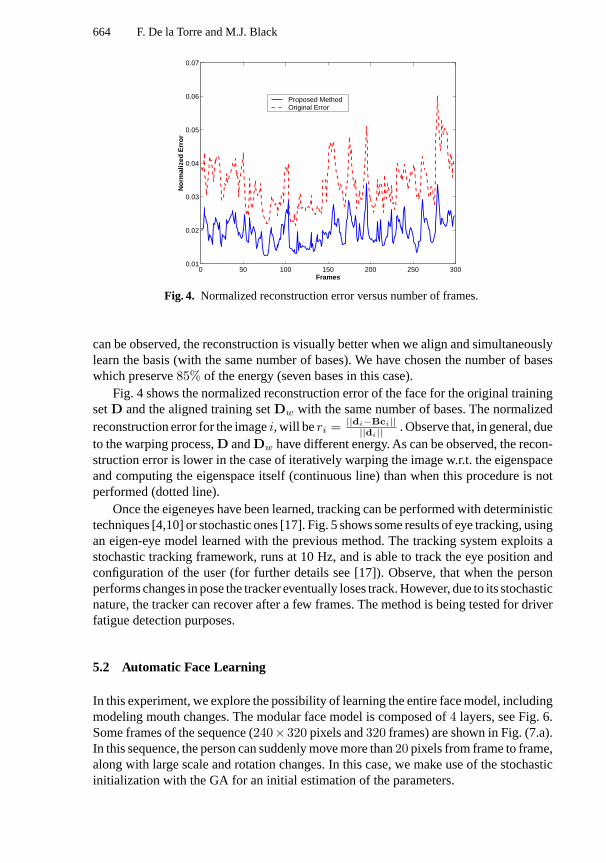
Fig. 4. Normalized reconstruction error versus number of frames.

can be observed, the reconstruction is visually better when we align and simultaneouslylearn the basis (with the same number of bases). We have chosen the number of baseswhich preserve85% of the energy (seven bases in this case).

Fig. 4 shows the normalized reconstruction error of the face for the original trainingsetD and the aligned training setDw with the same number of bases. The normalizedreconstruction error for the imagei, will beri = ||di−Bci||

||di|| . Observe that, in general, dueto the warping process,D andDw have different energy. As can be observed, the recon-struction error is lower in the case of iteratively warping the image w.r.t. the eigenspaceand computing the eigenspace itself (continuous line) than when this procedure is notperformed (dotted line).

Once the eigeneyes have been learned, tracking can be performed with deterministictechniques [4,10] or stochastic ones [17]. Fig. 5 shows some results of eye tracking, usingan eigen-eye model learned with the previous method. The tracking system exploits astochastic tracking framework, runs at 10 Hz, and is able to track the eye position andconfiguration of the user (for further details see [17]). Observe, that when the personperforms changes in pose the tracker eventually loses track. However, due to its stochasticnature, the tracker can recover after a few frames. The method is being tested for driverfatigue detection purposes.

5.2 Automatic Face Learning

In this experiment, we explore the possibility of learning the entire face model, includingmodeling mouth changes. The modular face model is composed of4 layers, see Fig. 6.Some frames of the sequence (240×320 pixels and320 frames) are shown in Fig. (7.a).In this sequence, the person can suddenly move more than20 pixels from frame to frame,along with large scale and rotation changes. In this case, we make use of the stochasticinitialization with the GA for an initial estimation of the parameters.


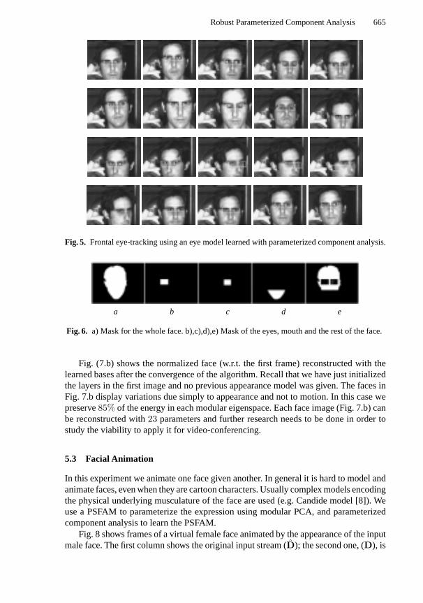
Fig. 5. Frontal eye-tracking using an eye model learned with parameterized component analysis.

a b c d e

Fig. 6. a) Mask for the whole face. b),c),d),e) Mask of the eyes, mouth and the rest of the face.

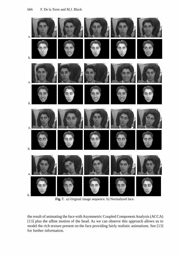
Fig. (7.b) shows the normalized face (w.r.t. the first frame) reconstructed with thelearned bases after the convergence of the algorithm. Recall that we have just initializedthe layers in the first image and no previous appearance model was given. The faces inFig. 7.b display variations due simply to appearance and not to motion. In this case wepreserve85% of the energy in each modular eigenspace. Each face image (Fig. 7.b) canbe reconstructed with23 parameters and further research needs to be done in order tostudy the viability to apply it for video-conferencing.

5.3 Facial Animation

In this experiment we animate one face given another. In general it is hard to model andanimate faces, even when they are cartoon characters. Usually complex models encodingthe physical underlying musculature of the face are used (e.g. Candide model [8]). Weuse a PSFAM to parameterize the expression using modular PCA, and parameterizedcomponent analysis to learn the PSFAM.

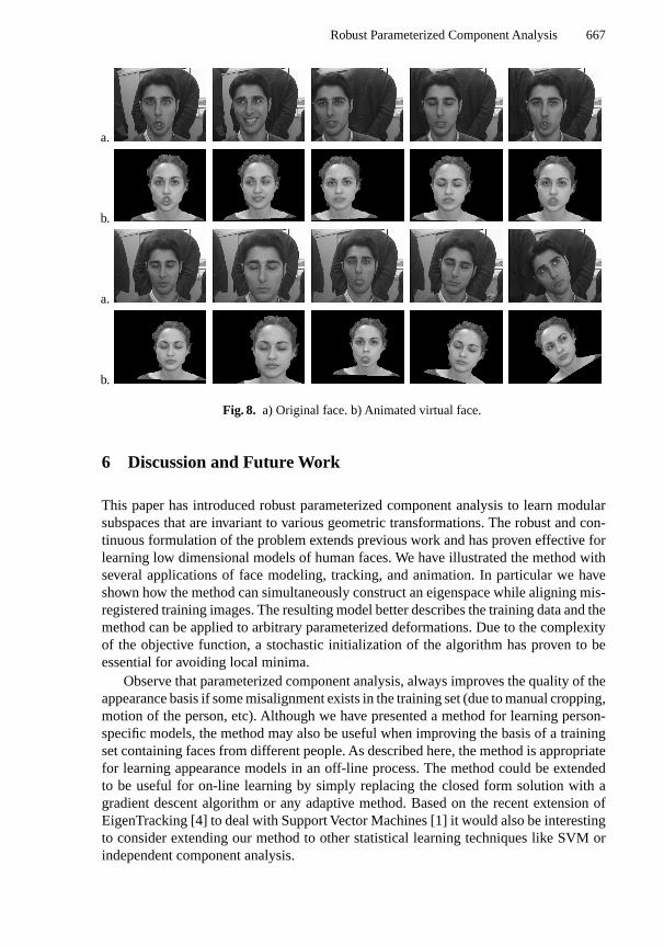
Fig. 8 shows frames of a virtual female face animated by the appearance of the inputmale face. The first column shows the original input stream (D); the second one, (D), is


a.

b.

a.

b.

a.

b.

a.

b.Fig. 7. a) Original image sequence. b) Normalized face.

the result of animating the face withAsymmetric Coupled ComponentAnalysis (ACCA)[13] plus the affine motion of the head. As we can observe this approach allows us tomodel the rich texture present on the face providing fairly realistic animations. See [13]for further information.


a.

b.

a.

b.

Fig. 8. a) Original face. b) Animated virtual face.

6 Discussion and Future Work

This paper has introduced robust parameterized component analysis to learn modularsubspaces that are invariant to various geometric transformations. The robust and con-tinuous formulation of the problem extends previous work and has proven effective forlearning low dimensional models of human faces. We have illustrated the method withseveral applications of face modeling, tracking, and animation. In particular we haveshown how the method can simultaneously construct an eigenspace while aligning mis-registered training images. The resulting model better describes the training data and themethod can be applied to arbitrary parameterized deformations. Due to the complexityof the objective function, a stochastic initialization of the algorithm has proven to beessential for avoiding local minima.

Observe that parameterized component analysis, always improves the quality of theappearance basis if some misalignment exists in the training set (due to manual cropping,motion of the person, etc). Although we have presented a method for learning person-specific models, the method may also be useful when improving the basis of a trainingset containing faces from different people. As described here, the method is appropriatefor learning appearance models in an off-line process. The method could be extendedto be useful for on-line learning by simply replacing the closed form solution with agradient descent algorithm or any adaptive method. Based on the recent extension ofEigenTracking [4] to deal with Support Vector Machines [1] it would also be interestingto consider extending our method to other statistical learning techniques like SVM orindependent component analysis.


Modeling the face with modular eigenspaces coupled by the motion can result in theloss of correlations between the parts (e.g. when smiling some wrinkles appear in the eyeregion). Now we are working on modeling the face with symmetric coupled componentanalysis [13] and are experimenting with hierarchical component analysis in which oneset of coefficients models the coupling between regions while each individual region hasits own coefficients for local variation.

Finally, the work presented in this paper on automatic learning of 2D PSFAMs hasthe limitation of being applicable to some particular view of the face, in this case thefrontal view. We are working on extending the PSFAM to model 3D changes withinthe same continuous optimization framework described here. Also, we are exploringimproving the 2D model (e.g. adding a more complex geometric transformation thattakes into account chin deformations).

Videos with the results for all the experiments performed in this paper can be down-loaded from http://www.salleURL.edu/∼ftorre/.

Acknowledgements. The first author has been partially supported by a grant from thethe Direccio General de Recerca of the Generalitat of Catalunya (#2001BEAI200220).This research was also supported by the DARPA HumanID project (ONR contractN000140110886) and a gift from the Xerox Foundation. We would like to thank Al-lan Jepson for discussions on robust PCA and eigen-registration.

References

1. S. Avidan. Support vector tracking. InConference on Computer Vision and Pattern Recogni-tion, 2001.

2. M. Betke and N. Makris. Fast object recognition in noisy images using simulated annealing.In International Conference Computer Vision, pages 523–530, 1994.

3. M. J. Black, D. J. Fleet, and Y. Yacoob. Robustly estimating changes in image appearance.Computer Vision and Image Understanding, 78(1):8–31, 2000.

4. M. J. Black and A. D. Jepson. Eigentracking: Robust matching and tracking of objects usingview-based representation.International Journal of Computer Vision, 26(1):63–84, 1998.

5. M. J. Black and Y. Yacoob. Recognizing facial expressions in image sequences using localparameterized models of image motion.International Journal of Computer Vision, 25(1):23–48, 1997.

6. A. Blake and M. Isard.Active Contours. Springer Verlag, 1998.7. A. Blake and A. Zisserman.Visual Reconstruction. MIT Press series, Massachusetts, 1987.8. M. Brand. Voice puppetry. InSIGGRAPH, pages 21–28, 1999.9. R. Cipolla and A. Pentland.Computer vision for Human-Machine Interaction. Cambridge

university press, 1998.10. T. F. Cootes, G. J. Edwards, and C. J. Taylor. Active appearance models. InEuropean Con-

ference Computer Vision, pages 484–498, 1998.11. T. F. Cootes and C. J. Taylor. Statistical models of appearance for com-puter vision. InWorld

Wide Web Publication, February 2001. (Available fromhttp://www.isbe.man.ac.uk/bim/refs.html).

12. F. de la Torre. Automatic learning of appearance face models. InSecond International Work-shop on Recognition, Analysis and Tracking of Faces and Gestures in Real-time Systems,pages 32–39, 2001.


13. F. de la Torre and M. J. Black. Dynamic coupled component analysis. InComputer Visionand Pattern Recognition, 2001.

14. F. de la Torre and M. J. Black. Robust principal component analysis for computer vision. InInternational Conference on Computer Vision, pages 362–369, 2001.

15. F. de la Torre, S. Gong, and S. McKenna. View alignment with dynamically updated affinetracking. InInt. Conf. on Automatic Face and Gesture Recognition, pages 510–515, 1998.

16. F. de la Torre, J. Vitri`a, P. Radeva, and J. Melench´on. Eigenfiltering for flexible eigentracking.In International Conference on Pattern Recognition, pages 1118–1121, Barcelona, 2000.

17. F. de la Torre, Y. Yacoob, and L. Davis. A probabilisitc framework for rigid and non-rigidappearance based tracking and recognition. InInt. Conf. on Automatic Face and GestureRecognition, pages 491–498, 2000.

18. K. I. Diamantaras.Principal Component Neural Networks (Therory and Applications). JohnWiley & Sons, 1996.

19. G. J. Edwards, A. Lanitis, C. Taylor, and T. F. Cootes. Statistical models of face images-improving specificity.Image and Vision Computing, 16:203–211, 1998.

20. G. J. Edwards, C. J. Taylor, and T.F. Cootes. Improving identitification performance by inte-grating evidence from sequences. InComputer Vision and Pattern Recognition, pages 486–491, 1999.

21. B. J. Frey and N. Jojic. Transformation-invariant clustering and dimensionality reduction.Submitted to IEEE Transaction on Pattern Analysis and Machine Intelligence, 2000.

22. S. Geman and D. McClure. Statistical methods for tomographic image reconstruction.Bulletinof the International Statistical Institute, LII:4:5, 1987.

23. S. Gong, S. Mckenna, and A. Psarrou.Dynamic Vision: From Images to Face Recognition.Imperial College Press, 2000.

24. G. Hager and P. Belhumeur. Efficient region tracking with parametric models of geometry andillumination.IEEE Transactions on Pattern Analysis and Machine Intelligence, 20(10):1025–1039, 1998.

25. F. Hampel, E. Ronchetti, P. Rousseeuw, and W. Stahel.Robust Statistics: The Approach Basedon Influence Functions. Wiley, New York., 1986.

26. T. Jebara, K. Russell, and A. Pentland. Mixtures of eigenfeatures for real-time structure fromtexture. InInternational Conference on Computer Vision, 1998.

27. A. Lanitis, A. Hill, T. F. Cootes, and C. J. Taylor. Locating facial feature using genetic algo-rithms. InInternational Conference on Digital Signal Processing, pages 520–525, 1995.

28. G. Li. Robust regression. In D. C. Hoaglin, F. Mosteller, and J. W. Tukey, editors,ExploringData, Tables, Trends and Shapes. John Wiley & Sons, 1985.

29. M. Mitchell.An Introduction to Genetic Algorithms. MIT Press, 1996.30. B. Moghaddam and A. Pentland. Probabilistic visual learning for object representation.Pat-

tern Analysis and Machine Intelligence, 19(7):137–143, July 1997.31. S. K. Nayar and T. Poggio.Early Visual Learning. Oxford University Press, 1996.32. R. P. N. Rao. Development of localized oriented receptive fields by learning a translation-

invariant code for natural images.Network: Comput. Neural Systems, 9:219–234, 1998.33. H. Schweitzer. Optimal eigenfeature selection by optimal image registration. InConference

on Computer Vision and Pattern Recognition, pages 219–224, 1999.34. M. Turk and A. Pentland. Eigenfaces for recognition.Journal Cognitive Neuroscience,

3(1):71–86, 1991.

robust parameterized component analysis

Documents