role of the plasmapause in dictating the ground

Role of the plasmapause in dictating the groundaccessibility of ELF/VLF chorus

D. I. Golden,1 M. Spasojevic,1 F. R. Foust,1 N. G. Lehtinen,1 N. P. Meredith,2

and U. S. Inan1,3

Received 21 July 2010; revised 23 August 2010; accepted 2 September 2010; published 17 November 2010.

[1] This study explores the manner in which the plasmapause is responsible fordictating which magnetospheric source regions of ELF/VLF chorus are able to propagate toand be received by midlatitude stations on the ground. First, we explore the effects ofplasmapause extent on ground‐based observations of chorus via a 3 month study ofground‐based measurements of chorus at Palmer Station, Antarctica (L = 2.4, 50°Sgeomagnetic latitude), and data on the plasmapause extent from the IMAGE EUVinstrument. It is found that chorus normalized occurrence peaks when the plasmapause isat L ∼ 2.6, somewhat higher than Palmer’s L shell, and that this occurrence peakpersists across a range of observed chorus frequencies. Next, reverse ray tracing isemployed to evaluate the portion of the equatorial chorus source region, distributed inradial distance and wave normal, from which chorus is able to reach Palmer Station viapropagation in a nonducted mode. The results of ray tracing are similar to those ofobservations, with a peak of expected occurrence when the plasmapause is at L ∼ 3.The exact location of the peak is frequency dependent. This supports the conclusionthat the ability of chorus to propagate to low altitudes and the ground is a strongfunction of instantaneous plasmapause extent and that peak occurrence of chorus at agiven ground station may occur when the L shell of the plasmapause is somewhat beyondthat of the observing station. These results also suggest that chorus observed on theground at midlatitude stations propagates predominantly in the nonducted mode.

Citation: Golden, D. I., M. Spasojevic, F. R. Foust, N. G. Lehtinen, N. P. Meredith, and U. S. Inan (2010), Role of theplasmapause in dictating the ground accessibility of ELF/VLF chorus, J. Geophys. Res., 115, A11211,doi:10.1029/2010JA015955.

1. Introduction

[2] Extremely low frequency/very low frequency (ELF/VLF) chorus emissions are electromagnetic waves which arespontaneously generated in the Earth’s magnetosphere.Chorus is characterized as consisting of repeating, usuallyrising and often overlapping coherent tones and is oftenaccompanied by a band of hiss [e.g., Cornilleau‐Wehrlin etal., 1978]. In recent years, chorus has received increasedattention due to the role that it is thought to play in theacceleration [e.g., Meredith et al., 2002; Horne et al., 2003,2005] and loss [e.g., Lorentzen et al., 2001; O’Brien et al.,2003; Thorne et al., 2005; Shprits et al., 2006] of energeticelectrons in the Earth’s radiation belts. Additionally, somefraction of chorus may act via its evolution into plasma-spheric hiss [Parrot et al., 2004; Santolík et al., 2006;Bortnik et al., 2008] as an additional loss agent for energetic

electrons [e.g., Lyons et al., 1972; Lyons and Thorne, 1973;Abel and Thorne, 1998; Meredith et al., 2007].[3] Chorus waves are believed to be generated by a

Doppler‐shifted cyclotron interaction between anisotropicdistributions of energetic >40 keV electrons and ambientbackground VLF noise [Tsurutani and Smith, 1974, 1977;Thorne et al., 1977]. These unstable distributions can resultfrom substorm injection, and correspondingly, chorus ispredominantly observed across the morning and noon localtime sectors in association with eastward drifting electrons.Because magnetic substorms both increase the flux of hotsource electrons which generate chorus as well as enhancethe auroral electrojet (AE), increases in the AE index havebeen shown to be a good predictor of chorus occurrencewithin the inner magnetosphere [Smith et al., 1999;Meredithet al., 2001]. The outer dayside region of the magnetosphereis also conducive to chorus generation, but here waves areless dependent on substorm activity and can be observedunder both quiet and disturbed geomagnetic conditions[Tsurutani and Smith, 1977; Li et al., 2009; Spasojevic andInan, 2010].[4] Ground‐based measurements of ELF/VLF emissions

are by definition limited to the small subset of space‐based

1STAR Laboratory, Stanford University, Stanford, California, USA.2British Antarctic Survey, Natural Environment Research Council,

Cambridge, UK.3Electrical Engineering Department, Koç University, Istanbul, Turkey.

Copyright 2010 by the American Geophysical Union.0148‐0227/10/2010JA015955

JOURNAL OF GEOPHYSICAL RESEARCH, VOL. 115, A11211, doi:10.1029/2010JA015955, 2010

A11211 1 of 15

http://dx.doi.org/10.1029/2010JA015955

emissions that are able to penetrate to low altitudes andthrough the ionosphere [e.g., Sonwalkar, 1995, pp. 424–425]. Ground‐based observations may include (1) wavesthat have propagated such that their wave normals naturallyarrive within the transmission cone at the ionosphericboundary [Helliwell, 1965, section 3.7], (2) waves that havepropagated within field‐aligned density irregularities knownas “ducts” [e.g., Smith, 1961; Carpenter, 1966; Carpenterand Sulic, 1988], which have the effect of constraining thewave normals to be nearly field aligned, or (3) waves thatarrive at the ionospheric boundary with nonvertical wavenormals and are then scattered from low‐altitude meter‐scaledensity irregularities [Sonwalkar and Harikumar, 2000] thatrotate the wave normals into the transmission cone.[5] In situ measurements of chorus have shown that

chorus occurs in two bands, separated by half the equatorialgyrofrequency ( fceq) along the observation field line[Tsurutani and Smith, 1974; Burtis and Helliwell, 1976;Tsurutani and Smith, 1977]. Of the two bands, only thelower band is thought to reach the ground; the upper band isbelieved to reflect at high altitudes due to its highly obliquewave normal angle [Hayakawa et al., 1984; Haque et al.,2010]. Thus, chorus received on the ground is expected tobe exclusively lower band chorus, generated below half theequatorial gyrofrequency.[6] The current work is motivated by a recent statistical

study by Golden et al. [2009] of chorus and hiss observed onthe ground at Palmer Station, Antarctica, at L = 2.4, 50°Sgeomagnetic latitude. During the course of that study, whichspanned 10 months in 2003, chorus was observed on morethan 50% of days. This was unexpected for several reasons.First, chorus is generated outside the plasmasphere, accord-ing to early satellite studies [e.g., Gurnett and O’Brien,1964; Dunckel and Helliwell, 1969] which have shownthat chorus is most commonly observed outside the plas-masphere. In addition, chorus observed on the ground hastraditionally been interpreted as a ducted emission, andtherefore, that the L shell on which it is received is approx-imately the same as the L shell on which it is generated. Thepresumption that nonducted chorus cannot penetrate to theground [e.g., Imhof et al., 1989, p. 10,092] is based on raytracing results that show that nonducted whistlers willmagnetospherically reflect before returning to the ground[Kimura, 1966; Edgar, 1976] and is supported by occasionalobservation of chorus‐like noise bursts that, in groundobservations, appear to have been triggered [Carpenteret al., 1975] or damped [Gail and Carpenter, 1984] byducted whistlers (implying that the observed whistlers andchorus share the same duct). However, in the study ofGolden et al. [2009], the magnetospheric conditions weresuch that the plasmapause was often expected to be wellbeyond Palmer’s L shell during chorus observations. Duringthat study, chorus was observed for Kp ] 2+. According tothe plasmapause model of Carpenter and Anderson [1992],at Kp = 2+, the plasmapause is expected to be around L ∼ 4.5.It is only for Kp > 6+ that the plasmapause is expected toreach down to L < 2.5. Also, the frequency range of observedchorus suggests that the source region of the waves is wellbeyond Palmer’s L shell. Satellite studies have shown thatlower band chorus is generated for frequencies in the range0.1 fceq ≤ f ≤ 0.5 fceq [Tsurutani and Smith, 1974; Burtis andHelliwell, 1976]. Waves of frequencies below 500 Hz were

observed by Golden et al. [2009], which corresponds to asource location of L > 5.5 under a dipole model of the Earth’smagnetic field.[7] It seems clear that the observations of Golden et al.

[2009] are inconsistent with the theory of ducted propaga-tion of chorus and that the dominant mode of chorus receptionat midlatitude stations like Palmer may instead be nonducted.In support of this possibility, Chum and Santolík [2005] haveshown via ray tracing that nonducted chorus, generated in theequatorial magnetosphere with wave normal angles near thelocal Gendrin angle, may be able to reach the ionosphere andpenetrate to the ground at L shells significantly below those atwhich the waves are generated. Although Chum and Santolík[2005] did not include a plasmasphere in their analysis, itseems logical, given the exoplasmaspheric source of chorusand the location of Palmer within the plasmasphere, that thelocation of the plasmapause may play an important role indetermining which subsets of chorus may be able to bereceived at Palmer.[8] In this study, we address two broad questions. (1) What

is the location of the plasmapause when chorus is observed atPalmer? (2) How does the location of the plasmapause affectthe portion of the chorus source region that is able to prop-agate to the ground and be received at Palmer? Thesequestions are answered via a combination of (1) a 3 monthstatistical study of chorus observations using the StanfordELF/VLF wave receiver at Palmer Station coupled withsimultaneous measurements of the plasmapause using theExtreme Ultraviolet (EUV) instrument on board the IMAGEsatellite and (2) a model‐based study of chorus propagationeffects via a new Stanford VLF 3‐D ray tracing softwarepackage, used to model magnetospheric propagation andLandau damping under different models of the plasmapauselocation, as well as a full wave code, used to model elec-tromagnetic propagation in the Earth‐ionosphere waveguide.

2. Experimental Methodology

[9] In order to determine the location of the plasmapausewhen chorus is observed at Palmer Station, we employ twoseparate databases: a database of emissions observed atPalmer Station and a database of plasmapause locations atPalmer’s MLT. Both databases span 3 months, from Aprilthrough June 2001, and are discussed below.

2.1. Palmer Emission Database

[10] Palmer Station is located on Anvers Island, near thetip of the Antarctic peninsula, at 64.77°S, 64.05°W, withIGRF geomagnetic parameters of L = 2.4, 50°S geomag-netic latitude, and magnetic local time (MLT) = UTC − 4.0at 100 km altitude. The Palmer VLF receiver records broad-band VLF data at 100 kilosamples per second using twocross‐loop magnetic field antennas, with 96 dB of dynamicrange. This analysis uses the North/South channel exclu-sively, it being the less subjectively noisy of the two channels;this has the additional effect of focusing Palmer’s viewingarea more tightly to its magnetic meridian than if bothchannels were used. Data products used in this study are 10 sbroadband data files, subsampled at a rate of 20 kilosamplesper second, beginning every 15 min at 5, 20, 35, and 50 minpast the hour, 24 h per day.

GOLDEN ET AL.: PLASMAPAUSE AND CHORUS A11211A11211

2 of 15

[11] The year 2001 falls approximately on the peak ofSolar Cycle 23, and chorus occurrence is frequent at PalmerStation during this period. A combination of automatedemission detection (D. I. Golden and M. Spasojevic, Deter-mination of solar cycle variations of midlatitude ELF/VLFchorus and hiss via automated signal detection, submitted toJournal of Geophysical Research, 2010) and manual cor-rection is used to determine the presence of emissions. Theautomated detector rejects confounding impulsive electro-magnetic signals, such as sferics and whistlers, and focuseson chorus and hiss. Chorus is then distinguished from hissbased on its “burstiness,” namely, the frequency content ofthe amplitude modulation of the broadband signal. Burstysignals are classified as chorus, and nonbursty signals areclassified as hiss, and discarded. The output of the automateddetector is then manually verified to eliminate false positives(e.g., hiss or lightning‐generated whistlers erroneouslylabeled as chorus) and false negatives (e.g., weak chorusemissions that may have been rejected based on their prox-imity to sferics or other emissions). Although it is likely thatsome chorus emissions with low signal‐to‐noise ratios areerroneously rejected by this algorithm, the profusion ofdetected chorus emissions still leads to statistically signif-icant results.[12] We define a “synoptic epoch” as an interval during

which Palmer data is sampled for this study. Each universalhour contains four synoptic epochs, at 5, 20, 35, and 50 minpast the hour. At each synoptic epoch, a binary judgment ismade about whether chorus is observed or not, based on theresults of both the automated detector and manual inspec-tion. The resulting table of true/false values for chorusobservation versus time then becomes the database ofPalmer chorus emissions. As an overview, Figure 1 shows acumulative spectrogram of the chorus emissions used in thisstudy. The cumulative spectrogram is effectively the loga-rithmic sum of the spectrums of its constituent emissions,and is a measure of the average chorus spectrum withrespect to frequency and local time. The full procedure isdescribed by Golden et al. [2009, section 2.2]. The gap at∼1.7 kHz on the cumulative spectrogram is a result ofincreased attenuation below the first transverse electric (TE1)waveguide mode cutoff during propagation in the Earth‐ionosphere waveguide. Only emissions in the boxed region,in the range 4 ≤ MLT ≤ 10 are used in this study.

2.2. Plasmapause Location Database

[13] In order to determine the instantaneous plasmapauselocation at each synoptic epoch, data from the Extreme

Ultraviolet (EUV) instrument [Sandel et al., 2000] on boardthe IMAGE satellite [Burch, 2000] are used. The EUVinstrument images resonantly scattered sunlight from He+

ions, which are a minority constituent of the plasma in theEarth’s plasmasphere. The He+ edge, as seen by the EUVinstrument, has been shown to be an accurate proxy for theplasmapause [Goldstein et al., 2003], which is the region ofthe magnetosphere where the electron density exhibits asteep drop with increasing L value.[14] Because this study focuses on emissions observed on

the ground at Palmer, the extent of the plasmapause is onlyconsidered at Palmer’s magnetic local time, MLT = UTC −4.0. Raw EUV images are initially mapped to the equatorialplane using the minimum L technique of Roelof and Skinner[2000, section 2.2], assuming a dipole model for the Earth’smagnetic field. The radial extent of the plasmapause is thenmanually selected on each individual EUV image at MLT =UTC − 4.0 and that plasmapause value is added to thedatabase. EUV images where the plasmapause cannot befound due to excessive noise or EUV camera malfunction,or where the plasmapause is either poorly defined or notvisible below L = 6, are discarded. After removing data gapsfrom both databases, 1033 synoptic epochs, or approxi-mately 260 h of data, remain for this study.

3. Dependence of Chorus Observations onPlasmapause Extent

3.1. Choice of AE Metric

[15] Since this study concerns the role of the plasmapausein dictating the observation of chorus emissions, it isinstructive to make mention of how the plasmapause iscorrelated with the AE index, which is itself well correlatedwith the observation of chorus emissions [e.g., Meredith etal., 2001]. This is done to explore a potential confoundingeffect where a single event, namely a magnetic substorm,may have two simultaneous consequences: (1) enhancementof the auroral electrojet, causing an increase in AE, and (2)erosion of the plasmasphere.[16] Figure 2 shows the extent of the plasmapause, sam-

pled at 04 ≤ MLT ≤ 10, MLT = UTC − 4.0, plotted againstthe instantaneous AE index (left), and the average AE in the

Figure 1. Cumulative spectrogram of chorus emissionsfrom April through June 2001. Only emissions in the boxedarea, between 04 and 10 MLT, are used in this study.

Figure 2. L shell of plasmapause at MLT = UTC − 4.0within the range 04 ≤ MLT ≤ 10 plotted against (left)instantaneous AE and (right) average AE in the previous12 hours. Plasmapause extent is moderately correlated withinstantaneous AE (r = −0.43, serr = 0.75 L) and highly cor-related with average AE in the previous 12 hours (r = −0.81,serr = 0.49 L). In each plot, the solid red line is a linear fitbetween plasmapause L and the logarithm of AE.


3 of 15

previous 12 hours (right), over the 3 month period of thisstudy. Averaging the AE index over N = 12 hours yieldsapproximately the greatest correlation for any value of N.The plasmapause is moderately correlated with the log ofinstantaneous AE, with correlation coefficient r = −0.43 andresidual standard deviation serr = 0.75 L, and highly corre-lated with the log of the average AE in the previous 12 hours,with correlation coefficient r = −0.81 and residual standarddeviation serr = 0.49 L.[17] However, the manner in which AE is associated with

plasmapause extent differs from how it is expected to beassociated with chorus occurrence. The time between whenAE is enhanced and when chorus is expected to be seen atPalmer may be determined by calculating the expected timerequired for a chorus source particle to drift from 00 MLTto 06 MLT. Based on work by Walt [1994, Figure B.2],100 keV electrons at L = 4 will drift from midnight to06 MLT in ∼21 min; higher‐energy particles will drift morequickly. This time period is on the order of the synopticepoch used in this study (15 min). Therefore instantaneousAE is used as the metric for predicting chorus in this study. Itis significant that, while instantaneous AE is expected to be agood predictor of chorus occurrence, it is only weakly cor-related with plasmapause extent. This suggests that sourceeffects, as measured by instantaneous AE, and propagationeffects, as measured by plasmapause extent, may exertindependent control over the probability that chorus will beseen at Palmer at any given time.

3.2. Chorus Occurrence Versus Plasmapause Extent

[18] Here the dependence of chorus normalized occurrenceon plasmapause extent is examined. The additional compli-cation of AE is deferred to the multivariate analysis ofsection 3.3. Although the detailed structure of the plasma-pause boundary layer is complex [Carpenter and Lemaire,2004], the major plasmapause structure is assumed to befield aligned over much of its range. For the purposes of thisstudy, the plasmapause can therefore be described via thescalar quantity LPP, which represents the equatorial plasma-pause extent, in units of Earth radii. A scatterplot of chorusobservations at each synoptic epoch versus instantaneousAE and LPP is shown in Figure 3. Synoptic epochs with

chorus are indicated with blue squares and epochs withoutchorus are indicated with red dots. The scattered pointsthemselves are the same as in the left panel of Figure 2,with some data gaps removed. One can get the generalimpression from this plot that chorus is more likely to beobserved at Palmer for low LPP and high AE. To examinethe data more rigorously, regression analysis is used toconstruct a generalized linear model [e.g., Chatterjee andHadi, 2006] of chorus normalized occurrence as a func-tion of plasmapause extent. This provides additionalinsight into properties that are not obvious from a simplescatterplot, such as at which LPP chorus occurrence ismaximized, and how strong that peak is.[19] Under regression analysis, a linear combination of

parameters is sought to form an estimate of m, the proba-bility of chorus occurrence. Because linear models have, ingeneral, unbounded values, a logit response function is usedfor m, defining the output of the linear model, Y, as

Y ¼ log�

1� �

� �ð1Þ

and, conversely,

� ¼ eY

1þ eY: ð2Þ

This transforms the bounded parameter m 2 [0, 1] to theunbounded parameter Y 2 (−∞, ∞). Given p distinct inde-pendent variables, Y is modeled as

Y ¼ X� ¼ 1; x1; x2; . . . ; xp½ �

�0

�1

�2

..

.

�p

26666666666664

37777777777775

; ð3Þ

where X is a row vector of predictors, formed by transfor-mations of the independent variables (e.g., x1 = LPP, x2 =LPP2 , etc.), and b is a column vector of coefficient estimates.[20] The generalized linear model regression procedure

from the MATLAB software package is used to obtain alinear fit. Although it is possible to include an arbitrarynumber of powers of LPP in the model, we honor the principleof parsimony and favor simpler models. Bayesian Informa-tion Criterion (BIC) [Chatterjee and Hadi, 2006, section12.6] is employed for this purpose, which assigns any par-ticular model a lower score for better goodness of fit, and ahigher score for each included term; lower scores are favored.Additionally, the maximum model order is restricted to 4.[21] To determine whether there is any frequency depen-

dence in the degree to which chorus occurrence changes withLPP, the regression analysis is separately performed on threecases: all frequencies, f < 1.5 kHz and f > 3 kHz. For allfrequencies and f < 1.5 kHz, the fourth‐order model has thelowest BIC and is therefore the favored model. For f > 3 kHz,the second‐order model has the lowest BIC. The modelparameters for the three cases, along with the p values, are

Figure 3. Scatterplot of synoptic epochs with (blue squares)and without (red dots) chorus. Note that AE is displayed ona logarithmic scale, while plasmapause extent is displayedon a linear scale.


4 of 15

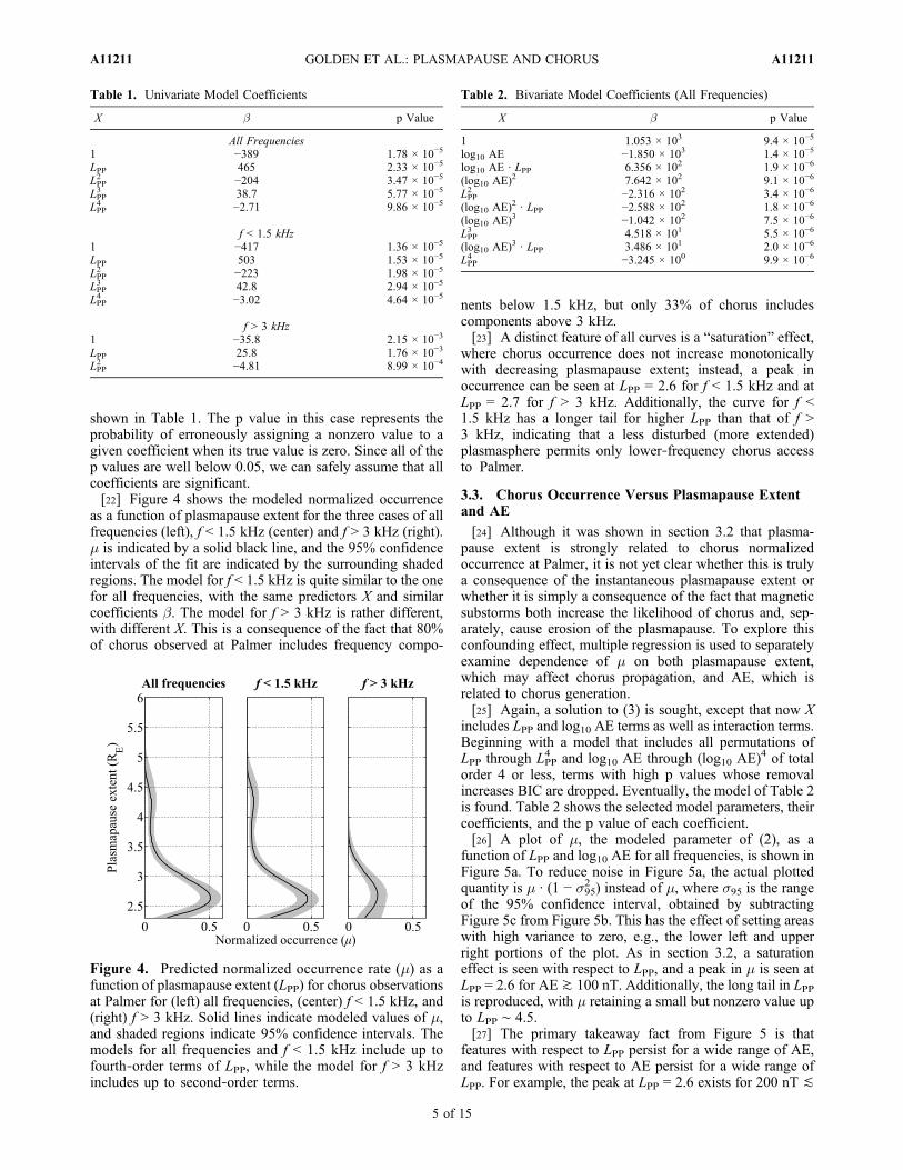
shown in Table 1. The p value in this case represents theprobability of erroneously assigning a nonzero value to agiven coefficient when its true value is zero. Since all of thep values are well below 0.05, we can safely assume that allcoefficients are significant.[22] Figure 4 shows the modeled normalized occurrence

as a function of plasmapause extent for the three cases of allfrequencies (left), f < 1.5 kHz (center) and f > 3 kHz (right).m is indicated by a solid black line, and the 95% confidenceintervals of the fit are indicated by the surrounding shadedregions. The model for f < 1.5 kHz is quite similar to the onefor all frequencies, with the same predictors X and similarcoefficients b. The model for f > 3 kHz is rather different,with different X. This is a consequence of the fact that 80%of chorus observed at Palmer includes frequency compo-

nents below 1.5 kHz, but only 33% of chorus includescomponents above 3 kHz.[23] A distinct feature of all curves is a “saturation” effect,

where chorus occurrence does not increase monotonicallywith decreasing plasmapause extent; instead, a peak inoccurrence can be seen at LPP = 2.6 for f < 1.5 kHz and atLPP = 2.7 for f > 3 kHz. Additionally, the curve for f <1.5 kHz has a longer tail for higher LPP than that of f >3 kHz, indicating that a less disturbed (more extended)plasmasphere permits only lower‐frequency chorus accessto Palmer.

3.3. Chorus Occurrence Versus Plasmapause Extentand AE

[24] Although it was shown in section 3.2 that plasma-pause extent is strongly related to chorus normalizedoccurrence at Palmer, it is not yet clear whether this is trulya consequence of the instantaneous plasmapause extent orwhether it is simply a consequence of the fact that magneticsubstorms both increase the likelihood of chorus and, sep-arately, cause erosion of the plasmapause. To explore thisconfounding effect, multiple regression is used to separatelyexamine dependence of m on both plasmapause extent,which may affect chorus propagation, and AE, which isrelated to chorus generation.[25] Again, a solution to (3) is sought, except that now X

includes LPP and log10 AE terms as well as interaction terms.Beginning with a model that includes all permutations ofLPP through LPP

4 and log10 AE through (log10 AE)4 of total

order 4 or less, terms with high p values whose removalincreases BIC are dropped. Eventually, the model of Table 2is found. Table 2 shows the selected model parameters, theircoefficients, and the p value of each coefficient.[26] A plot of m, the modeled parameter of (2), as a

function of LPP and log10 AE for all frequencies, is shown inFigure 5a. To reduce noise in Figure 5a, the actual plottedquantity is m · (1 − s95

2 ) instead of m, where s95 is the rangeof the 95% confidence interval, obtained by subtractingFigure 5c from Figure 5b. This has the effect of setting areaswith high variance to zero, e.g., the lower left and upperright portions of the plot. As in section 3.2, a saturationeffect is seen with respect to LPP, and a peak in m is seen atLPP = 2.6 for AE^ 100 nT. Additionally, the long tail in LPPis reproduced, with m retaining a small but nonzero value upto LPP ∼ 4.5.[27] The primary takeaway fact from Figure 5 is that

features with respect to LPP persist for a wide range of AE,and features with respect to AE persist for a wide range ofLPP. For example, the peak at LPP = 2.6 exists for 200 nT ]

Table 1. Univariate Model Coefficients

X b p Value

All Frequencies1 −389 1.78 × 10−5

LPP 465 2.33 × 10−5

LPP2 −204 3.47 × 10−5

LPP3 38.7 5.77 × 10−5

LPP4 −2.71 9.86 × 10−5

f < 1.5 kHz1 −417 1.36 × 10−5

LPP 503 1.53 × 10−5

LPP2 −223 1.98 × 10−5

LPP3 42.8 2.94 × 10−5

LPP4 −3.02 4.64 × 10−5

f > 3 kHz1 −35.8 2.15 × 10−3

LPP 25.8 1.76 × 10−3

LPP2 −4.81 8.99 × 10−4

Figure 4. Predicted normalized occurrence rate (m) as afunction of plasmapause extent (LPP) for chorus observationsat Palmer for (left) all frequencies, (center) f < 1.5 kHz, and(right) f > 3 kHz. Solid lines indicate modeled values of m,and shaded regions indicate 95% confidence intervals. Themodels for all frequencies and f < 1.5 kHz include up tofourth‐order terms of LPP, while the model for f > 3 kHzincludes up to second‐order terms.

Table 2. Bivariate Model Coefficients (All Frequencies)

X b p Value

1 1.053 × 103 9.4 × 10−5

log10 AE −1.850 × 103 1.4 × 10−5

log10 AE · LPP 6.356 × 102 1.9 × 10−6

(log10 AE)2 7.642 × 102 9.1 × 10−6

LPP2 −2.316 × 102 3.4 × 10−6

(log10 AE)2 · LPP −2.588 × 102 1.8 × 10−6

(log10 AE)3 −1.042 × 102 7.5 × 10−6

LPP3 4.518 × 101 5.5 × 10−6

(log10 AE)3 · LPP 3.486 × 101 2.0 × 10−6

LPP4 −3.245 × 100 9.9 × 10−6


5 of 15

AE ] 1000 nT, and the peak at AE = 500 nT exists for2.1 ] LPP ] 3.1. This is an indication that effects of AE orLPP near the peak of chorus occurrence are quasi‐indepen-dent of each other. Had it been otherwise, and the effects ofAE and LPP were strongly dependent, the peak in Figure 5would appear as a diagonal line. Therefore, it is clear thatthe plasmapause is in fact significantly changing the char-acteristics of chorus propagation to Palmer, and that thecorrelation between LPP and m is not merely a confoundingeffect of the fact that magnetic substorms tend to affect bothchorus generation and the plasmapause.

4. Modeling of Chorus Propagation

[28] The effects of plasmapause extent on chorus propa-gation are further investigated using a combination of raytracing and full wave modeling. First, reverse ray tracing isused wherein rays begin above the ionosphere over Palmerwith wave normal angles within the ionospheric transmis-sion cone. The rays are then propagated backward to theirmagnetospheric source. A valid source location for each rayis outside the plasmasphere at the magnetic equatorial plane[LeDocq et al., 1998; Santolík et al., 2005] at a radialdistance such that the wave frequency is in the range 0.1fceq ≤ f ≤ 0.5 fceq [Tsurutani and Smith, 1974; Burtis andHelliwell, 1976]. Rays that are able to enter a valid sourcelocation are binned by radial extent and wave normal angle.This creates a comprehensive picture of the portion of theequatorial source region from which generated rays mayreach Palmer. Ray attenuation is calculated via Landaudamping on the magnetospheric ray paths using an empiricalmodel of energetic particle fluxes. In addition, we assumethat waves may penetrate the ionosphere some distance fromPalmer and propagate within the Earth‐ionosphere wave-guide before being received; a full wave model is used toestimate this additional waveguide attenuation. Full detailsof the simulation are further discussed below. The simulationis performed for a range of plasmapause extents. For each

plasmapause extent, a single scalar quantity is calculated,which we term the Chorus Availability Factor (CHAF).CHAF is a cumulative measure of the portion of the chorussource region, integrated over all radial extents and wavenormals, and weighted by relative attenuation and sourceprobability, that is observable at Palmer. Although CHAF isnot a probability, if the plasmapause extent does significantlyinfluence chorus propagation, the trends of CHAF versus LPPare expected to resemble those of the experimentally mod-eled chorus normalized occurrence, m, from section 3.2.

4.1. Stanford VLF 3‐D Ray Tracer

[29] The new version of the Stanford VLF ray tracer wasdeveloped by one of us (F. R. F.) as a more accurate andcomplete model to replace Stanford’s previous ray tracingprogram [Inan and Bell, 1977], which we refer to as theStanford VLF legacy ray tracer. The new ray tracer, whichwe refer to as the Stanford VLF 3‐D ray tracer, was writtenfrom the ground up, and is not an extension or revision ofthe Stanford VLF legacy ray tracer. A description of the raytracer follows.[30] Hamilton’s equations for the propagation of a ray

through a medium with spatially varying dispersion relationdefined by the implicit function F(w, k, r) = 0 can be statedas

drdt

¼ � rkF

@F=@!ð4Þ

dkdt

¼ rrF

@F=@!ð5Þ

with the constraint

F !;k; rð Þ ¼ 0: ð6Þ

For generality, and for the purpose of accommodating anyarbitrary function for the plasma density or backgroundmagnetic field, the spatial and k‐space derivatives areevaluated numerically using finite differences; that is,

@F

@ki� 1

2DkF !; k þDkei; rð Þ � F !;k �Dkei; rð Þð Þ ð7Þ

@F

@ri� 1

2DrF !;k; rþDreið Þ � F !; k; r�Dreið Þð Þ; ð8Þ

where i = {1, 2, 3}, and ei are the unit vectors. Since thederivatives are evaluated numerically, all that is required toadapt a new plasma density model is a function that eval-uates F(w, k, r).[31] After approximating the spatial and k‐space deriva-

tives, six ordinary differential equations remain, which areintegrated numerically in time using a standard adaptiveRunge‐Kutta method. In contrast to the approach ofHaselgrove [1955], a moving B0‐aligned coordinate systemis not used; instead, the system of equations is directly solvedin global Cartesian coordinates. After one time step, theconstraint F = 0 is not in general met, and an intermediatesolution exists with an error F(w, k*, r*) = �. This is handledusing a standard method for solving constrained ODEs, by

Figure 5. Model for m, the normalized occurrence rateof chorus as a function of plasmapause extent and AE,obtained using generalized linear model regression onobservations of chorus. (a) The expected value of normalizedoccurrence. (b) Upper and (c) lower bounds of the 95%confidence interval for m.


6 of 15

finding a “nearby” point (k, r) that satisfies F(w, k, r) = 0 afterevery time step. The specific approach used is to simplyre‐solve the dispersion relation assuming the wave normalangle is kept constant. If this fails (due to being too close tothe resonance cone), the time step is halved and the proce-dure is attempted again.[32] The Stanford VLF 3‐D ray tracer can accommodate

any arbitrary function for the cold background plasmanumber density. In this study, the Global Core Plasma Model(GCPM) [Gallagher et al., 2000] is implemented, sampledon a regular grid and interpolated by a fast, local, C1 (con-tinuous in the first derivative) tricubic interpolation schemedescribed by Lekien and Marsden [2005]. The plasmaspheremodeled by the GCPM is field aligned to the dipole field, andremains so from the equatorial region down to altitudesbetween 7800 km (Kp ∼ 3+) to 2600 km (Kp ∼ 8−). Thetypical plasmapause represented by the GCPM exhibits adensity drop of between 1 (Kp ∼ 3+) and 1.5 (Kp ∼ 8−) ordersof magnitude in the equatorial plane over a range of about0.3 RE. The choice of background magnetic field is alsoarbitrary; in this study, the Tsyganenko‐96 (T96) model[Tsyganenko, 1995; Tsyganenko and Stern, 1996] is used.[33] Thermal losses are included as in work by Kennel

[1966]. Equation (3.9) by Kennel [1966], corrected for atypographical error [Chen et al., 2009, paragraph 9], issolved for the Landau (m = 0) resonance. This yields thetemporal damping rate wi, which is then related to the spatialdamping rate ki by the relation by Brinca [1972]:

!i ¼ ki!� vg!: ð9Þ

The method by Kennel [1966] requires the evaluation of thegradients of the hot particle distribution function in (vk, v?)space, as well as the evaluation of a 1‐D integral over v?over the interval [0, ∞). In order to accommodate anyarbitrary distribution function, the derivatives are againevaluated numerically using finite differences. The velocityis first normalized by the speed of light for numerical rea-sons, then mapped into a finite range t = (0, 1) using themapping v? = (1 − t)/t:

Z 1

0f v?ð Þdv? ¼

Z 1

0

1

t2f

1� t

t

� �dt: ð10Þ

Finally, the integral is evaluated numerically using adaptivequadrature. The method used is general and can accom-modate any number of resonances. In this study, only theLandau (m = 0) resonance is used, since it is the dominantsource of loss.[34] The choice of hot particle distribution is crucial to the

accurate calculation of Landau damping. Within the plas-masphere, the phase space density expression of Bell et al.[2002], based on measurements with the POLAR space-craft sampled in the range 2.3 < L < 4, is used. Outside theplasmasphere, the methodology of Bortnik et al. [2007a],derived from measurements with the CRRES spacecraftoutside the plasmasphere up to L ∼ 7, is used.[35] A hybrid model smooths the two models at the

plasmasphere boundary, and is implemented as follows. Letf0POL represent the phase space density (PSD) of Bell et al.[2002] from POLAR in units of, e.g., s3/cm6, and let f0

CRR

represent the PSD of Bortnik et al. [2007a] from CRRES in

the same units. Define the “weights” of the two distributionsat a given L shell, Lmeas, for a given plasmapause extent,LPP, as

wPOL ¼ exp �� Lmeas � LPPð Þð Þ1þ exp �� Lmeas � LPPð Þð Þ

wCRR ¼ exp � Lmeas � LPPð Þð Þ1þ exp � Lmeas � LPPð Þð Þ :

ð11Þ

Then, the implemented hybrid PSD is given by the weightedmean in log‐space of POLAR and CRRES PSDs as

f hybrid0 ¼ explog f POL0

� �wPOL þ log f CRR0

� �wCRR

wPOL þ wCRR

� �: ð12Þ

[36] Reasonable results are obtained with a = 5. For ref-erence, when Lmeas − LPP = 0, the two distributions areweighted equally in log‐space, and when Lmeas − LPP = +(−)0.5, i.e., the measurement location is 0.5 L shells beyond(within) the plasmapause, f 0

CRR is weighted 12 times more(less) than f 0POL in log‐space.[37] It should be noted that, although this ray tracing

procedure is three dimensional, the following study isrestricted to rays that lie approximately in a single meridi-onal plane. Due to azimuthal gradients in the plasma and Bfield models, rays exhibit a slight tendency to propagate toearlier local times with increasing L shell. The maximumazimuthal deviation of any ray considered in this study is18° (1.2 hours in MLT), with an average maximal deviationper ray of 7° (0.5 hours in MLT). Because this value issmall, the local time deviation of rays is neglected in thisstudy, and wave normals and positions are given in twodimensions with respect to the meridional plane of the rays.

4.2. Ray Tracing Procedure

[38] Rays are launched in the vicinity of Palmer, at l =50°S, MLT = 06, UT = 10. The GCPM and Tsyganenkomodels for plasma density and magnetic field are used, andthe rays propagate in the nonducted mode. Rays are launchedat 1000 km altitude, with 80 equally spaced magnetic lati-tudes within 1000 km of 50°S, and with 13 equally spaced kvector angles directed away from the Earth within thetransmission cone, for a total of 1040 rays per simulation.[39] The transmission cone angle defines the maximum

deviation of downward‐directed k vectors, with respect tothe normal to the Earth’s surface, that may penetrate throughthe ionosphere and to the ground without suffering totalinternal reflection at the boundary between the lower edgeof the ionosphere and free space [e.g., Helliwell, 1965,section 3.7]. To calculate the transmission cone, it isassumed that the plasma density from the ray origin to theground may be approximated as a stratified medium, andtherefore that the horizontal component of the k vector isconserved. At 1 kHz and 4 kHz, two frequencies of interestfor this study, the half angle of the transmission cone,measured from the vertical, is 0.84° and 1.44°, respectively.[40] Each ray is traced for up to 30 s or until it either

impacts the Earth or departs from the precalculated densitygrid in the range −4 ≤ XSM ≤ 4, −8 ≤ YSM ≤ 0, −3 ≤ ZSM ≤ 3,where all coordinates are in units of Earth radii in the solar‐magnetic coordinate system. In practice, under these criteria,


7 of 15

no rays survive beyond 10 s. Each time a ray crosses theequatorial plane, the local plasma density and gyrofrequencyare examined. If the ray is (1) outside the plasmasphere and(2) within the range 0.1 fceq ≤ f ≤ 0.5 fceq (where fceq is theequatorial electron gyrofrequency along the given fieldline), which is the frequency range of lower band chorus[Tsurutani and Smith, 1974; Burtis and Helliwell, 1976],then that point is saved as a potential chorus source location.A single original ray may give rise to more than onepotential chorus source location if it exhibits multiplemagnetospheric reflections.[41] The chorus source region (i.e., the region from which

chorus is truly generated, which is not the same as thelocation from which the “reverse” rays are launched) isconsidered to lie on the equatorial plane, with initial wavenormal angles uniformly distributed within the resonancecone. Although several satellite studies have attempted tocharacterize the wave normal distribution of the equatorialchorus source [e.g., Haque et al., 2010, and referencestherein], statistics have generally been too low to draw anydefinitive conclusions, leading to our use of a uniform dis-tribution in this study. The source region is binned on twoparameters: R, the distance from the center of the Earth inthe equatorial plane, and y, the initial wave normal angle

with respect to the ambient magnetic field. Each bin is ofuniform size, with DR = 0.05 RE and Dy = 4°.[42] Chorus rays that can reach Palmer tend to occur in

several distinct “families,” or groupings of rays with similarinitial wave normals and radial extent. Figure 6 shows sev-eral facets of the ray tracing procedure, along with examplerays from the two ray families that are present at 1 kHz. Forthis simulation, LPP = 2.9. The ray tracing procedure isdescribed below with reference to Figure 6.[43] Figure 6a shows representative rays from the two ray

families. We interpret the rays in their “forward” sense, as ifthey were originally launched from the equatorial plane andeventually arrived at 1000 km altitude. Ray paths are shownin white, with wave normals shown as red ticks, equallyspaced every 100 ms. The magenta line indicates a contourof f /fceq = 0.1; all chorus generation happens at values of Rbeyond this boundary. The upper bound on fceq for chorusgeneration, at f/fceq = 0.5 is beyond the scale of the image, atR ∼ 7 RE. Palmer’s location is indicated by the green triangleat l = −50° on the surface of the Earth. The backgroundimage is a meridional slice of the GCPM electron density.Ray family 1 consists of rays that propagate directly fromthe chorus source region to Palmer without magneto-spherically reflecting (MR), and family 2 consists of raysthat MR at the plasmapause boundary, which allows them

Figure 6. Two 1 kHz ray families that are capable of being received at Palmer. (a) Representativeraypaths from each of two ray families. Family 1 is the direct path from the source region to Palmer,and family 2 includes rays that magnetospherically reflect into the plasmasphere before their receptionon the ground. (b) Initial refractive index surfaces for example rays. (c) Attenuation of example raysversus time over the course of ray tracing, via Landau damping. (d) Attenuation of example rays versusdistance within the Earth‐ionosphere waveguide, via full wave modeling. (e) Source factor showing rel-ative expected chorus versus radial extent. (f) Source attenuation plot of relative received power versuswave normal y and radial extent. Solid lines indicate the local resonance cone angle, yres, and dashedlines indicate the local Gendrin angle, yg. The two families of similar rays, labeled 1 and 2, correspondto the two example rays from the previous panels.


8 of 15

access into the plasmapause before reaching Palmer.Because ray tracing is performed in three dimensions, theray paths and wave normals have been projected into theMLT = 06 meridional plane.[44] Figure 6b shows the initial refractive index surfaces

for the representative rays. The direction of the ambientmagnetic field, B0, the wave refractive index, np = c/vp, andthe group refractive index, ng = c/vg, as well as the Gendrinangle, yg, are indicated, where c is the speed of light in freespace, vp is the wave phase velocity and vg is the wave groupvelocity. np and ng point in the direction of the wave kvector and group velocity vector, respectively.[45] Each potential chorus source location represents a ray

that originally begins with unity power and is attenuated intwo separate steps. First, Figure 6c shows the attenuation ofthe representative rays over the course of their magneto-spheric propagation due to Landau damping, as discussed insection 4.1. The majority of damping occurs at high L shellsoutside the plasmasphere. In particular, once ray 2 enters theplasmasphere, the attenuation due to Landau damping isnegligible. Unlike some other studies of ray tracing [e.g.,Bortnik et al., 2007a, 2007b], this study does not include ageometric effect in determining the power gain or loss dueto the focusing of magnetic field lines at low altitudes.Instead, this focusing or defocusing happens naturallythrough the use of a large number of rays.[46] The second mode of attenuation, shown in Figure 6d,

is attenuation from Earth‐ionosphere waveguide propaga-tion. Each ray begins at 1000 km altitude with the injectionpoint footprint a distance d from Palmer Station, where d ≤1000 km. Earth‐ionosphere waveguide attenuation is cal-culated using the full wave model of Lehtinen and Inan[2008, 2009]. A summer nighttime ionospheric profile anda perfectly conducting ground layer (representative of Pal-mer’s primarily all‐sea paths) are used. A Gaussian wavepacket of the appropriate frequency is injected at 140 kmaltitude with vertical (downward) wave normal. The groundpower at various distances from the source is recorded,normalized by the ground power directly beneath the source.The resulting quantity A(d) represents an attenuation factorfor Earth‐ionosphere waveguide propagation, as a functionof d, by which each ray’s power is multiplied. The full wavemodel is run only once for any given frequency, and thequantity A(d) is assumed to be valid for all modeled rayswithin 1000 km of Palmer. The two example rays reach theground at ∼450 km and ∼215 km from Palmer, respectively,and are marked as such in Figure 6d. When both Landaudamping and Earth‐ionosphere waveguide attenuation areconsidered, there can be wide variations in the attenuation ofdifferent rays in a given family, due to the fact that slightvariations in initial conditions may give rise to large varia-tions in propagation paths and ionospheric penetrationpoints.[47] Figure 6e is a plot of “source factor” as a function of

radial extent, R. This plot is derived from work by Burtisand Helliwell [1976, Figure 9c], which shows chorusoccurrence as a function of f/fceq. We define source factor asthe observed occurrence of Burtis and Helliwell [1976,Figure 9c], normalized so that the maximum value is 1.Here, source factor is plotted against R, using the T96magnetic field model to map from f/fceq to R. The sourcefactor plot is then the relative expected likelihood of

observing a 1 kHz chorus source at a given radial extent inthe equatorial plane. Because the measurements of Burtisand Helliwell [1976] include both waves inside and out-side the plasmasphere, it is possible that the observed choruspercentage is artificially low at low f/fceq or R due to thosemeasurements being taken within the plasmasphere wherechorus is generally not observed. The use of the sourcefactor in deriving the Chorus Availability Factor (CHAF) isdiscussed in section 4.3, and due to the possible con-founding effects of its constituent data containing mea-surements inside the plasmasphere, CHAF is derived bothwith and without implementing the source factor.[48] After building a list of potential chorus source loca-

tions from the 1040 original rays, the amplitude of any givenR‐y bin is set to the maximum ray amplitude in that bin afterattenuation both via Landau damping in the magnetosphereand via attenuation in the Earth‐ionosphere waveguide. Werefer to a plot of the binned results for a simulation with agiven wave frequency and plasmapause extent as a “sourceattenuation plot.”[49] Figure 6f shows a source attenuation plot for a sim-

ulation where LPP = 2.9, from which the two example raysare drawn. The local resonance cone angle, yres, defined asthe wave normal angle at which the magnitude of therefractive index goes to infinity, is indicated by the solidblack lines. The local Gendrin angle, yg, defined as thenonzero wave normal angle at which the group velocityvector is parallel to the static magnetic field, is indicated bythe dashed black lines. The two separate ray families, fromwhich the above example rays are drawn, are highlightedwith red boxes. The rays do not show any particular rela-tionship with the resonance cone or Gendrin angles.[50] Figure 7 is analogous to Figure 6, but for 4 kHz

waves. Because f is increased, the magenta lines, indicatingthe contours of f/fceq = 0.1 and f/fceq = 0.5 are now closer tothe Earth, and both boundaries of the chorus source regioncan be seen. In addition, there are now four ray families,representing the direct path, and one, two and three magne-tospheric reflections. In all cases, the damping is most sig-nificant at large L shells outside the plasmasphere, wherewave normals are most oblique. Rays 3 and 4 begin withtheir wave normals directed away from the Earth, near theresonance cone. After the first magnetospheric reflection,they appear to be guided by the plasmapause boundarybefore reflecting from the inner boundary. This has the effectof rotating the wave normal toward the Earth, allowing therays to reach the ground. Because Rays 3 and 4 spend moretime outside the plasmasphere, and have more highly obliquewave normals than do rays 1 and 2, they are damped moreheavily during their propagation.[51] In the 4 kHz case, the initial wave normals of some

ray families do show a relationship with the resonance coneand Gendrin angles. Some rays from families 1 and 2 tend tobe generated near the Gendrin angle, while some rays fromfamilies 3 and 4 tend to be generated near the resonancecone angle. The associations are loose, and no ray familiesappear constrained to either the resonance cone or theGendrin angle. The relation between the wave normals ofray family 1 (the direct path) and the Gendrin angle isconsistent with the work of Chum and Santolík [2005], whofound that certain rays generated with wave normals in thevicinity of the Gendrin angle would reach low altitudes and


9 of 15

possibly penetrate to the ground before being magneto-spherically reflected. Although this behavior is seen in ourresults at 4 kHz, it is not observed at 1 kHz. This is possiblydue to the fact that Chum and Santolík [2005] did notinclude Landau damping in their calculations. Althoughsome 1 kHz rays in our study do begin at the equatorialplane with wave normals near the Gendrin angle, thosewaves are damped to negligible power in the simulation, andtherefore do not appear on the source attenuation plot inFigure 6f.

4.3. Chorus Availability Factor

[52] Figures 6f and 7f showed source attenuation plots at1 kHz and 4 kHz for a single plasmapause extent, LPP =2.9. This analysis is repeated for many different values of LPPto gain insight into the particular way in which the plasma-pause extent affects the ability for chorus waves to propagatefrom their source to Palmer. Figure 8 shows source attenu-ation plots for 1 kHz (upper panels) and 4 kHz (lower panels)for plasmapause extents in the range 2.1 ≤ LPP ≤ 4.3. Thecolor scale has been changed slightly for clarity.[53] Initially, we focus our discussion on the 1 kHz case,

in the upper panels of Figure 8. At the greatest plasmapauseextent, LPP = 4.3, rays from the chorus source region are notaccessible to Palmer; reverse rays launched from Palmer areeither unable to escape the plasmasphere, and instead reflect

off of its inner boundary before impacting the ionosphere inthe conjugate hemisphere, or they escape the plasmaspherewith oblique wave normals and are heavily damped beforecrossing the equatorial plane. As the plasmasphere becomesmore eroded down to LPP = 2.9, although rays as far out asL = 7 are accessible to Palmer (not shown), most areseverely damped; only certain rays that originate within4.2 ⪅ L ⪅ 4.6 sufficiently avoid damping to be receivedabove the −70 dB cutoff. Erosion of the plasmaspherebeyond LPP = 2.9 results in increased propagation time out-side the plasmasphere, and hence, increased damping, par-ticularly for waves with initial wave normals y ∼ 50°. Thesituation is similar for 4 kHz. For high LPP, rays from thechorus source region cannot reach Palmer; reverse rays areunable to escape the plasmasphere. For LPP ∼ 2.9, a maxi-mum of rays reach Palmer with significant power. For lowLPP, as for high LPP most reverse rays launched fromPalmer do not escape the plasmasphere.[54] One important difference between the simulations at

1 kHz and 4 kHz is where the plasmapause lies with respectto the extents of the chorus source region, defined by 0.1 ≤f/fceq ≤ 0.5. At 1 kHz, the source region is in the range4.2 ≤ L ≤ 6.9, which is beyond the plasmapause foralmost all simulations. However, at 4 kHz, the sourceregion is in the range 2.7 ≤ L ≤ 4.5, which means that formany of the simulations, the plasmasphere overlaps the

Figure 7. Same as Figure 6 but for 4 kHz. At this frequency, there are four distinct ray families,representing the direct path and one, two, and three magnetic reflections.


10 of 15

chorus source region. This is why, in the lower panels ofFigure 8, the chorus source region appears to expand tothe left as LPP decreases. The plasmapause is moving tothe left of the plots, and a greater portion of the chorussource region is becoming available.[55] Because rays may be substantially damped over the

course of propagation, in order to properly analyze theresults of the simulations, it is necessary to define a “mini-mum detectable ray power,” below which rays are excludedfrom the analysis. To first order, this can be achieved bycomparing the mean power observed on the ground with themean power observed via in situ measurements. A histogramof observed amplitudes over the course of this study, overlaidwith the associated probability distribution, is shown inFigure 9. Chorus amplitudes observed at Palmer are dis-tributed approximately lognormally, as

AdB � lnN � ¼ 3:5; �2 ¼ 0:036� �

; ð13Þ

with mean 35 dB‐fT and standard deviation 6.8 dB‐fT. Theobserved mean amplitude of 35 dB‐fT at Palmer can becompared with the mean B field amplitude calculated bySantolík [2008], based on equatorial chorus E field mea-surements fromMeredith et al. [2001], of 10–100 pT, or 80–100 dB‐fT. Comparing the two numbers, up to ∼65 dB ofattenuation is expected from the equatorial source region toPalmer. However, in this analysis, we are not modelingattenuation suffered through transionospheric propagation.Transionospheric attenuation is expected to be on the orderof ∼5 dB, somewhere between the daytime and nighttimeattenuation calculations of Helliwell [1965, Figure 3‐35], for2 kHz waves (since our simulations are run at 06 MLT). Thisleaves an expected attenuation from Landau damping andEarth‐ionosphere waveguide losses of ∼60 dB. To accountfor the lower end of our observed power distribution, whichreaches down to ∼25 dB‐fT in Figure 9, an additional 10 dBof loss is allowed. Thus, we define our minimum detectable

Figure 8. Source attenuation plots for (upper panels) f = 1 kHz and (lower panels) f = 4 kHz for plas-mapause extents in the range 2.1 ≤ LPP ≤ 4.3. Note that the scales of the x axes in the upper and lowerpanels are not the same.


11 of 15

ray power to be −70 dB. Although it is necessary to define aminimum detectable ray power to perform the followinganalysis, our conclusions are not strongly dependent on itsexact value.[56] We define the CHAF for a given frequency and LPP

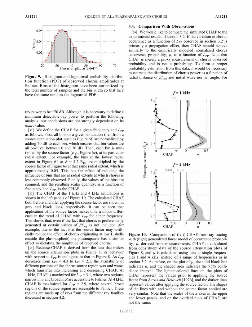
as follows. First, all bins of a given simulation (i.e., from asource attenuation plot, such as Figure 6f) are normalized byadding 70 dB to each bin, which ensures that bin values areall positive, between 0 and 70 dB. Then, each bin is mul-tiplied by the source factor (e.g., Figure 6e), at its particularradial extent. For example, the bins at the lowest radialextent in Figure 6f, at R ∼ 4.2 RE, are multiplied by thesource factor of Figure 6e at that same radial extent, which isapproximately 0.05. This has the effect of reducing theinfluence of bins that are at radial extents at which chorus isless commonly observed. Finally, the values of the bins aresummed, and the resulting scalar quantity, as a function offrequency and LPP, is the CHAF.[57] The CHAF of the 1 kHz and 4 kHz simulations is

shown in the left panels of Figure 10. The calculated CHAFboth before and after applying the source factor are shown ingray and black lines, respectively. It can be seen thatapplication of the source factor makes only a minor differ-ence in the trend of CHAF with LPP for either frequency.This shows that, even if the fact that chorus is preferentiallygenerated at certain values of f/fceq is not included (forexample, due to the fact that the source factor may artifi-cially reduce the effect of chorus originating at low L shellsoutside the plasmasphere) the plasmapause has a similareffect in dictating the amplitude of received chorus.[58] Because CHAF is derived from the data that makes

up the source attenuation plots in Figure 8, its behaviorwith respect to LPP is analogous to that in Figure 8. As LPPdecreases from LPP = 4.3 to LPP = 2.1, the availability ofdifferent portions of the chorus source region wax and wane,which translates into increasing and decreasing CHAF. At1 kHz, CHAF is maximized for LPP = 3.1, where two regions,narrow iny and broad inR are accessible to Palmer. At 4 kHz,CHAF is maximized for LPP = 2.9, where several broadregions of the source region are accessible to Palmer. Theseregions are made up of rays from the different ray familiesdiscussed in section 4.2.

4.4. Comparison With Observations

[59] We would like to compare the simulated CHAF to theexperimental results of section 3.2. If the variation in chorusoccurrence as a function of LPP observed in section 3.2 isprimarily a propagation effect, then CHAF should behavesimilarly to the empirically modeled normalized chorusoccurrence probability, m, as a function of LPP. Note thatCHAF is merely a proxy measurement of chorus observedprobability and is not a probability. To form a properprobability estimation from this data, it would be necessaryto estimate the distribution of chorus power as a function ofradial distance or f/fceq and initial wave normal angle. For

Figure 10. Comparison of (left) CHAF from ray tracingwith (right) generalized linear model of occurrence probabil-ity, m, derived from measurements. CHAF is calculatedfrom constituent data of the source attenuation plots ofFigure 8, and m is calculated using data at single frequen-cies 1 and 4 kHz, instead of a range of frequencies as insection 3.2. As before, on the plot of m, the solid black lineindicates m, and the shaded area indicates the 95% confi-dence interval. The lighter‐colored lines on the plots ofCHAF represent the values prior to applying the sourcefactor from Burtis and Helliwell [1976], and the darker linesrepresent values after applying the source factor. The shapesof the lines with and without the source factor applied arevery similar. Note that the scales of the x axes in the upperand lower panels, and on the overlaid plots of CHAF, arenot the same.

Figure 9. Histogram and lognormal probability distribu-tion function (PDF) of observed chorus amplitudes atPalmer. Bins of the histogram have been normalized bythe total number of samples and the bin width so that theyhave the same units as the lognormal PDF.


12 of 15

lack of this information, we have assumed uniform initialpower at all wave normals and radial distances.[60] Figure 10 shows a comparison of the CHAF at 1 and

4 kHz with the equivalent univariate generalized linearmodel (GLM) results for m. The GLM results shown hereare limited to chorus occurring at 1 and 4 kHz, instead of theranges f < 1.5 kHz and f > 3 kHz shown in Figure 4. First,and most importantly, the saturation effect is reproduced forboth frequencies. Both m and CHAF initially increase withdecreasing LPP, reach a peak, and then decrease. Their peaksare within 0.5 L. This similarity between CHAF and m isstrongly indicative of the fact that the behavior of m withrespect to LPP is a propagation effect and not a source effect(since only propagation effects are included in the raytracing).[61] However, we also note the important discrepancy

between the LPP values for the peaks of CHAF and the peaksof m. For 1 kHz, the peak of m is at LPP = 2.6, whereas thatfor CHAF is at LPP = 3.1, a difference of 0.5 RE. The ran-dom error in the measured value of LPP for either m (mea-sured by clicking on equatorially mapped EUV images) orCHAF (measured by direct examination of an equatorialslice through the GCPM grid) is estimated to be ±0.1 RE, butthis is too small to account for the observed discrepancy.Similarly for 4 kHz, the observed peaks are at LPP = 2.7 andLPP = 2.9, respectively, a smaller difference of 0.2 RE.[62] There are several different possible causes for the

discrepancy between the peaks in m and CHAF. The firstand most obvious cause may be errors in particle densitiesfrom the GCPM density model, either in the absolute den-sity or in density gradients. The GCPM model necessarilyrepresents “averaged” conditions for its input values, andmay contain systematic biases with respect to the truemagnetospheric conditions under which chorus is observedat Palmer.[63] Another cause may lie in our use of a hybrid ener-

getic electron distribution when calculating Landau damp-ing. The CRRES distribution used outside the plasmasphereuses data from disturbed periods, when AE > 300 nT.However, the POLAR distribution used inside the plasma-sphere uses data from quiet‐to‐moderate conditions, whenKp ≤ 4. Because chorus tends to peak during active periods,the use of quiet/moderate fluxes within the plasmaspherehas the effect of artificially lowering the energetic particleflux inside the plasmasphere, therefore lowering the damp-ing coefficients and allowing rays to propagate for a longtime within the plasmasphere. Thus, at 1 kHz, ray family 2from Figure 6, which involves extended propagation withinthe plasmasphere, and which is dominant for LPP ^ 2.7, maybe less influential than modeled.[64] Finally, by excluding the prevalent density irregu-

larities that permeate the plasmasphere [e.g., Carpenteret al., 2002, and references therein], we neglect what maybe a significant population of waves that are guided by theseirregularities. In particular, in the real plasmasphere, densityirregularities in the vicinity of the plasmapause may prefer-entially guide waves to Palmer when the plasmapause is atlower L shells [Inan and Bell, 1977]. The exclusion ofirregularities is an inevitable consequence of using an“averaged” plasma density model, such as the GCPM modelfor the plasma density. A full discussion of the effects of

guiding by density irregularities is beyond the scope of thisstudy.[65] One other important discrepancy between the plots

of m and CHAF is that the relative value of m for lowfrequencies is significantly greater than that for high fre-quencies (right panels), whereas the opposite relation is truefor CHAF (left panels). This may be due to the fact thathigher‐frequency waves tend to be generated with loweramplitudes [Burtis and Helliwell, 1975], whereas we haveassumed in our ray tracing analysis that the amplitude ofgenerated waves is the same across all frequencies.

5. Conclusions

[66] We have proposed in this study that the extent of theplasmapause, denoted LPP, plays a large role in determiningthe ability for chorus waves to propagate from their equa-torial magnetospheric source region to the ground. Usingwave data from the ground‐based receiver at Palmer Station,Antarctica, together with plasmapause data from the IMAGEEUV instrument, a generalized linear model regression wasemployed in section 3.2 to show the strong dependence ofchorus normalized occurrence on LPP.[67] The separability of AE and LPP shown in section 3.3

provides evidence that the dependence of chorus occurrenceon LPP is in fact a propagation effect, and not simply aconfounding source effect (i.e., a consequence of the fact thatmagnetic substorms both give rise to chorus generation and,separately, cause erosion of the plasmasphere). In particular,Figure 5 shows that the general trend of normalized occur-rence versus plasmapause persists across a wide range of AEvalues. This shows that the relation of chorus occurrence toAE (a proxy measure of a source effect), is separable fromthe relation of chorus occurrence to LPP (a measure of apropagation effect), and therefore, that there is a significantinfluence of instantaneous plasmapause extent in determin-ing whether chorus can reach Palmer.[68] These conclusions were solidified via a reverse ray

tracing study. By launching rays from Palmer and trackingtheir power, wave normal, and equatorial crossings throughthe expected chorus source region, a measure of the portionof the chorus source region from which rays may reachPalmer was obtained, which we termed the Chorus Avail-ability Factor, or CHAF. The most salient similarity betweenhow the experimentally observed chorus occurrence (m) andthe ray tracing model (CHAF) depend on LPP is the so‐calledsaturation effect, where during experimental observations,chorus is observed on the ground most often for L ∼ 2.6. Itwas shown in section 4.4 that this effect is reproduced via raytracing (with a small systematic error in the exact value ofLPP) by varying only LPP; this eliminates the possibility of aconfounding source effect, and further enforces the con-clusion that the plasmapause extent has a direct effect onallowing chorus access to the ground.[69] The peak of the saturation, either the observed peak

of 2.6 ] LPP ] 2.7 or the modeled peak of 2.9 ] LPP ] 3.1,is somewhat higher than Palmer’s location at L = 2.4. Onemight naïvely expect the peak of chorus to occur at LPP =2.4, because it is at that plasmasphere extent that PalmerStation lies on the plasmapause boundary. However, thistheory neglects the mechanism of rays reaching Palmer viamagnetospherically reflecting at the plasmapause boundary,


13 of 15

as in ray family 2 from Figure 6 and ray families 2, 3, and 4from Figure 7. This can occur at high plasmapause extents,and the prevalence of this mode of propagation may be oneexplanation for why chorus is often observed at Palmereven when the plasmapause is beyond L = 2.4.[70] Additionally, by ray tracing in a smooth magneto-

sphere (except for the obvious density gradient of theplasmapause itself), it was shown that it is possible forchorus to reach the ionosphere within the transmission coneand penetrate to the ground in the absence of any field‐aligned guiding structures. This is in contrast to long‐heldcolloquial belief that only ducted chorus may access theground. In fact, in light of the similarities between the raytracing and the experimentally observed results, it seemsplausible that nonducted chorus is the dominant mode ofchorus observed on the ground. Without the constraint of afield‐aligned guiding structure, chorus is able to cross Lshells as it propagates from the source region to the ground.This explains why Palmer Station, located at a significantlylower L shell than that of the typical chorus source region, isable to observe chorus as often as it does.[71] We conclude by saying that, due to the fact that

midlatitude ground observations of chorus are likely toresult from nonducted propagation, these observations areby no means limited to chorus source regions that lie on thesame L shell as the receiver. In addition, plasmapause extentis an often neglected but critically important factor indetermining chorus propagation to low altitudes and theground.

[72] Acknowledgments. The work at Stanford University was sup-ported by the National Science Foundation under award 0538627 and theOffice of Naval Research under awards N00014‐09‐1‐0034 and Z882802.[73] Robert Lysak thanks Yuri Shprits and another reviewer for their

assistance in evaluating this paper.

ReferencesAbel, B., and R. M. Thorne (1998), Electron scattering loss in Earth’s innermagnetosphere: 1. Dominant physical processes, J. Geophys. Res., 103,2385–2396, doi:10.1029/97JA02919.

Bell, T. F., U. S. Inan, J. Bortnik, and J. D. Scudder (2002), The Landaudamping of magnetospherically reflected whistlers within the plasma-sphere, Geophys. Res. Lett., 29(15), 1733, doi:10.1029/2002GL014752.

Bortnik, J., R. M. Thorne, and N. P. Meredith (2007a), Modeling the prop-agation characteristics of chorus using CRRES suprathermal electronfluxes, J. Geophys. Res., 112, A08204, doi:10.1029/2006JA012237.

Bortnik, J., R. M. Thorne, N. P. Meredith, and O. Santolík (2007b), Raytracing of penetrating chorus and its implications for the radiation belts,Geophys. Res. Lett., 34, L15109, doi:10.1029/2007GL030040.

Bortnik, J., R. M. Thorne, and N. P. Meredith (2008), The unexpected ori-gin of plasmaspheric hiss from discrete chorus emissions, Nature, 452,62–66, doi:10.1038/nature06741.

Brinca, A. L. (1972), On the stability of obliquely propagating whistlers,J. Geophys. Res., 77, 3495–3507, doi:10.1029/JA077i019p03495.

Burch, J. L. (2000), IMAGE mission overview, Space Sci. Rev., 91, 1–14.Burtis, W. J., and R. A. Helliwell (1975), Magnetospheric chorus: Ampli-tude and growth rate, J. Geophys. Res., 80, 3265–3270.

Burtis, W. J., and R. A. Helliwell (1976), Magnetospheric chorus:Occurrence patterns and normalized frequency, Planet. Space Sci., 24,1007–1007, doi:10.1016/0032-0633(76)90119-7.

Carpenter, D. L. (1966), Whistler studies of the plasmapause in the mag-netosphere: 1. Temporal variations in the position of the knee andsome evidence on plasma motions near the knee, J. Geophys. Res., 71,693–709.

Carpenter, D. L., and R. R. Anderson (1992), An ISEE/Whistler model ofequatorial electron density in the magnetosphere, J. Geophys. Res., 97,1097–1108, doi:10.1029/91JA01548.

Carpenter, D. L., and J. Lemaire (2004), The plasmasphere boundary layer,Ann. Geophys., 22, 4291–4298.

Carpenter, D. L., and D. M. Sulic (1988), Ducted whistler propagation out-side the plasmapause, J. Geophys. Res., 93, 9731–9742, doi:10.1029/JA093iA09p09731.

Carpenter, D. L., J. C. Foster, T. J. Rosenberg, and L. J. Lanzerotti (1975),A subauroral and midlatitude view of substorm activity, J. Geophys. Res.,80, 4279–4286.

Carpenter, D. L., et al. (2002), Small‐scale field‐aligned plasmasphericdensity structures inferred from the Radio Plasma Imager on IMAGE,J. Geophys. Res., 107(A9), 1258, doi:10.1029/2001JA009199.

Chatterjee, S., and A. S. Hadi (2006), Regression Analysis by Example, 4thed., Wiley‐Interscience, Hoboken, N. J.

Chen, L., J. Bortnik, R. M. Thorne, R. B. Horne, and V. K. Jordanova(2009), Three‐dimensional ray tracing of VLF waves in a magneto-spheric environment containing a plasmaspheric plume, Geophys. Res.Lett., 36, L22101, doi:10.1029/2009GL040451.

Chum, J., and O. Santolík (2005), Propagation of whistler‐mode chorus tolow altitudes: Divergent ray trajectories and ground accessibility, Ann.Geophys., 23, 3727–3738.

Cornilleau‐Wehrlin, N., R. Gendrin, F. Lefeuvre, M. Parrot, R. Grard,D. Jones, A. Bahnsen, E. Ungstrup, and W. Gibbons (1978), VLF elec-tromagnetic waves observed onboard GEOS‐1, Space Sci. Rev., 22,371–382.

Dunckel, N., and R. A. Helliwell (1969), Whistler‐mode emissions on theOGO 1 satellite, J. Geophys. Res., 74, 6371–6385, doi:10.1029/JA074i026p06371.

Edgar, B. C. (1976), The upper‐ and lower‐frequency cutoffs of magne-tospherically reflected whistlers, J. Geophys. Res., 81, 205–211,doi:10.1029/JA081i001p00205.

Gail, W. B., and D. L. Carpenter (1984), Whistler‐induced suppressionof VLF noise, J. Geophys. Res., 89, 1015–1022, doi:10.1029/JA089iA02p01015.

Gallagher, D. L., P. D. Craven, and R. H. Comfort (2000), Global coreplasma model, J. Geophys. Res., 105, 18,819–18,834, doi:10.1029/1999JA000241.

Golden, D. I., M. Spasojevic, and U. S. Inan (2009), Diurnal dependence ofELF/VLF hiss and its relation to chorus at L = 2.4, J. Geophys. Res., 114,A05212, doi:10.1029/2008JA013946.

Goldstein, J., M. Spasojević, P. H. Reiff, B. R. Sandel, W. T. Forrester,D. L. Gallagher, and B. W. Reinisch (2003), Identifying the plasmapausein IMAGE EUV data using IMAGE RPI in situ steep density gradients,J. Geophys. Res., 108(A4), 1147, doi:10.1029/2002JA009475.

Gurnett, D. A., and B. J. O’Brien (1964), High‐latitude geophysical studieswith satellite Injun 3: 5. Very low frequency electromagnetic radiation,J. Geophys. Res., 69, 65–89.

Haque, N., M. Spasojevic, O. Santolík, and U. S. Inan (2010), Wave nor-mal angles of magnetospheric chorus emissions observed on the Polarspacecraft, J. Geophys. Res., 115, A00F07, doi:10.1029/2009JA014717.

Haselgrove, J. (1955), Ray theory and a new method for ray tracing, in ThePhysics of the Ionosphere: Report of the Physical Society Conference onthe Physics of the Ionosphere Held at the Cavendish Laboratory, Cam-bridge, September, 1954, p. 355, Physical Soc., London.

Hayakawa, M., Y. Yamanaka, M. Parrot, and F. Lefeuvre (1984), The wavenormals of magnetospheric chorus emissions observed on board GEOS 2,J. Geophys. Res., 89, 2811–2821, doi:10.1029/JA089iA05p02811.

Helliwell, R. A. (1965), Whistlers and Related Ionospheric Phenomena,Stanford Univ. Press, Stanford, Calif.

Horne, R. B., S. A. Glauert, and R. M. Thorne (2003), Resonant diffusionof radiation belt electrons by whistler‐mode chorus, Geophys. Res. Lett.,30(9), 1493, doi:10.1029/2003GL016963.

Horne, R. B., et al. (2005), Wave acceleration of electrons in the Van Allenradiation belts, Nature, 437, 227–230, doi:10.1038/nature03939.

Imhof, W. L., H. D. Voss, J. Mobilia, M. Walt, and U. S. Inan (1989),Characteristics of short‐duration electron precipitation bursts and theirrelationship with VLF wave activity, J. Geophys. Res., 94, 10,079–10,093, doi:10.1029/JA094iA08p10079.

Inan, U. S., and T. F. Bell (1977), The plasmapause as a VLF wave guide,J. Geophys. Res., 82, 2819–2827, doi:10.1029/JA082i019p02819.

Kennel, C. (1966), Low‐frequency whistler mode, Phys. Fluids, 9,2190–2202, doi:10.1063/1.1761588.

Kimura, I. (1966), Effects of ions on whistler‐mode ray tracing, Radio Sci.,1(3), 269–283.

LeDocq, M. J., D. A. Gurnett, and G. B. Hospodarsky (1998), Chorussource locations from VLF Poynting flux measurements with the Polarspacecraft, Geophys. Res. Lett. , 25, 4063–4066, doi:10.1029/1998GL900071.

Lehtinen, N. G., and U. S. Inan (2008), Radiation of ELF/VLF waves byharmonically varying currents into a stratified ionosphere with applica-


14 of 15

tion to radiation by a modulated electrojet, J. Geophys. Res., 113,A06301, doi:10.1029/2007JA012911.

Lehtinen, N. G., and U. S. Inan (2009), Full‐wave modeling of transiono-spheric propagation of VLF waves, Geophys. Res. Lett., 36, L03104,doi:10.1029/2008GL036535.

Lekien, F., and J. Marsden (2005), Tricubic interpolation in three dimen-sions, Int. J. Numer. Methods Eng., 63, 455–471.

Li, W., et al. (2009), Global distribution of whistler‐mode chorus wavesobserved on the THEMIS spacecraft, Geophys. Res. Lett., 36, L09104,doi:10.1029/2009GL037595.

Lorentzen, K. R., J. B. Blake, U. S. Inan, and J. Bortnik (2001), Observa-tions of relativistic electron microbursts in association with VLF chorus,J. Geophys. Res., 106, 6017–6028, doi:10.1029/2000JA003018.

Lyons, L. R., and R. M. Thorne (1973), Equilibrium structure of radia-tion belt electrons, J. Geophys. Res., 78, 2142–2149, doi:10.1029/JA078i013p02142.

Lyons, L. R., R. M. Thorne, and C. F. Kennel (1972), Pitch‐angle diffusionof radiation belt electrons within the plasmasphere, J. Geophys. Res., 77,3455–3474.

Meredith, N. P., R. B. Horne, and R. R. Anderson (2001), Substorm depen-dence of chorus amplitudes: Implications for the acceleration of electronsto relativistic energies, J. Geophys. Res., 106, 13,165–13,178,doi:10.1029/2000JA900156.

Meredith, N. P., R. B. Horne, D. Summers, R. M. Thorne, R. H. A. Iles,D. Heynderickx, and R. R. Anderson (2002), Evidence for accelerationof outer zone electrons to relativistic energies by whistler mode chorus,Ann. Geophys., 20, 967–979.

Meredith, N. P., R. B. Horne, S. A. Glauert, and R. R. Anderson (2007),Slot region electron loss timescales due to plasmaspheric hiss and light-ning‐generated whistlers, J. Geophys. Res., 112, A08214, doi:10.1029/2007JA012413.

O’Brien, T. P., K. R. Lorentzen, I. R. Mann, N. P. Meredith, J. B. Blake,J. F. Fennell, M. D. Looper, D. K. Milling, and R. R. Anderson (2003),Energization of relativistic electrons in the presence of ULF powerand MeV microbursts: Evidence for dual ULF and VLF acceleration,J. Geophys. Res., 108(A8), 1329, doi:10.1029/2002JA009784.

Parrot, M., O. Santolík, D. Gurnett, J. Pickett, and N. Cornilleau‐Wehrlin(2004), Characteristics of magnetospherically reflected chorus wavesobserved by CLUSTER, Ann. Geophys., 22, 2597–2606.

Roelof, E. C., and A. J. Skinner (2000), Extraction of ion distributions frommagnetospheric ENA and EUV images, Space Sci. Rev., 91, 437–459.

Sandel, B. R., et al. (2000), The Extreme Ultraviolet Imager investigationfor the IMAGE mission, Space Sci. Rev., 91, 197–242.

Santolík, O. (2008), New results of investigations of whistler‐mode chorusemissions, Nonlinear Processes Geophys., 15, 621–630.

Santolík, O., D. A. Gurnett, J. S. Pickett, M. Parrot, and N. Cornilleau‐Wehrlin (2005), Central position of the source region of storm‐timechorus, Planet. Space Sci., 53, 299–305, doi:10.1016/j.pss.2004.09.056.

Santolík, O., J. Chum, M. Parrot, D. A. Gurnett, J. S. Pickett, and N.Cornilleau‐Wehrlin (2006), Propagation of whistler mode chorus to lowaltitudes: Spacecraft observations of structured ELF hiss, J. Geophys.Res., 111, A10208, doi:10.1029/2005JA011462.

Shprits, Y. Y., R. M. Thorne, R. B. Horne, S. A. Glauert, M. Cartwright,C. T. Russell, D. N. Baker, and S. G. Kanekal (2006), Accelerationmechanism responsible for the formation of the new radiation belt dur-ing the 2003 Halloween solar storm, Geophys. Res. Lett., 33, L05104,doi:10.1029/2005GL024256.

Smith, A. J., M. P. Freeman, M. G. Wickett, and B. D. Cox (1999), On therelationship between the magnetic and VLF signatures of the substormexpansion phase, J. Geophys. Res., 104, 12,351–12,360, doi:10.1029/1998JA900184.

Smith, R. L. (1961), Propagation characteristics of whistlers trapped infield‐aligned columns of enhanced ionization, J. Geophys. Res., 66,3699–3707, doi:10.1029/JZ066i011p03699.

Sonwalkar, V. S. (1995), Magnetospheric LF‐, VLF‐, and ELF‐waves, inHandbook of Atmospheric Electrodynamics, vol. 2, edited by H. Volland,pp. 407–460, CRC Press, Boca Raton, Fla.

Sonwalkar, V. S., and J. Harikumar (2000), An explanation of groundobservations of auroral hiss: Role of density depletions and meter‐scaleirregularities, J. Geophys. Res., 105, 18,867–18,884, doi:10.1029/1999JA000302.

Spasojevic, M., and U. S. Inan (2010), Drivers of chorus in the outer day-side magnetosphere, J. Geophys. Res., 115, A00F09, doi:10.1029/2009JA014452.

Thorne, R. M., S. R. Church, W. J. Malloy, and B. T. Tsurutani (1977), Thelocal time variation of ELF emissions during periods of substorm activ-ity, J. Geophys. Res., 82, 1585–1590.

Thorne, R. M., T. P. O’Brien, Y. Y. Shprits, D. Summers, and R. B. Horne(2005), Timescale for MeV electron microburst loss during geomagneticstorms, J. Geophys. Res., 110, A09202, doi:10.1029/2004JA010882.

Tsurutani, B. T., and E. J. Smith (1974), Postmidnight chorus: A substormphenomenon, J. Geophys. Res. , 79 , 118–127, doi :10.1029/JA079i001p00118.

Tsurutani, B. T., and E. J. Smith (1977), Two types of magnetosphericELF chorus and their substorm dependences, J. Geophys. Res., 82,5112–5128.

Tsyganenko, N. A. (1995), Modeling the Earth’s magnetospheric magneticfield confined within a realistic magnetopause, J. Geophys. Res., 100,5599–5612, doi:10.1029/94JA03193.

Tsyganenko, N. A., and D. P. Stern (1996), Modeling the global magneticfield of the large‐scale Birkeland current systems, J. Geophys. Res., 101,27,187–27,198, doi:10.1029/96JA02735.

Walt, M. (1994), Introduction to Geomagnetically Trapped Radiation,Cambridge Univ. Press, Cambridge, U. K.

F. R. Foust, D. I. Golden, N. G. Lehtinen, and M. Spasojevic, STARLaboratory, Stanford University, 350 Serra Mall, Packard Bldg., Stanford,CA 94305‐9515, USA. ([email protected])U. S. Inan, Electrical Engineering Department, Koç University, Sariyer

34450, Istanbul, Turkey. ([email protected])N. P. Meredith, British Antarctic Survey, Natural Environment Research

Council, Madingley Road, Cambridge CB3 0ET, UK. ([email protected])


15 of 15

role of the plasmapause in dictating the ground

Documents