ronald c. davidson intense self fieldphysics of charged … · · 2002-07-05ities based on...

Physics of Charged Particle Beams withIntense Self Field

Ronald C. Davidson

Plasma Physics Laboratory

Princeton University, Princeton, NJ 08543

Workshop on Advanced Accelerator Concepts

Mandalay Beach, California

June 23 – 28, 2002

∗Research supported by the U.S. Department of Energy.

Collaborators

➱ Theory:Hong Qin, Paul Channell, Igor Kaganovich, Wei-li Lee, Gennady Shvets,Edward Startsev, Sean Strasburg, Stephan Tzenov, and Tai-Sen Wang

➱ Experiment:Philip Efthimion, Eirk Gilson, Larry Grisham, and Richard Majeski.

Physics of Intense Charged Particle Beams

Background:

➱ A fundamental understanding of nonlinear effects and collective processeson the propagation, acceleration, and compression of high-brightness, high-intensity charged particle beam is essential to the identification of optimumoperating regimes in which emittance growth and beam losses are mini-mized.

➱ Collective processes and self-field effects become particularly important atthe high beam intensities and luminosities envisioned in present and next-generation accelerators and transport systems for applications in:

❍ High energy and nuclear physics.

❍ Heavy Ion Fusion.

Physics of Intense Charged Particle Beams

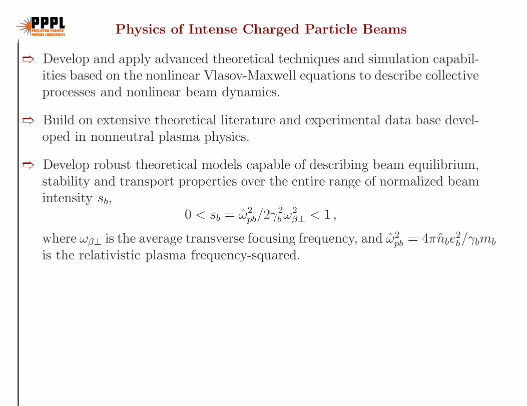
➱ Develop and apply advanced theoretical techniques and simulation capabil-ities based on the nonlinear Vlasov-Maxwell equations to describe collectiveprocesses and nonlinear beam dynamics.

➱ Build on extensive theoretical literature and experimental data base devel-oped in nonneutral plasma physics.

➱ Develop robust theoretical models capable of describing beam equilibrium,stability and transport properties over the entire range of normalized beamintensity sb,

0 < sb = ω2pb/2γ

2bω

2β⊥ < 1 ,

where ωβ⊥ is the average transverse focusing frequency, and ω2pb = 4πnbe

2b/γbmb

is the relativistic plasma frequency-squared.

What is Nonneutral Plasma?

➱ A nonneutral plasma is a many-body collection of charged particles in whichthere isn’t overall charge neutrality.

➱ Such systems are characterized by intense self-electric fields (space-chargefields), and in high-current configurations by intense self-magnetic fields.

➱ Examples of nonneutral plasma systems include:

❍ One-component nonneutral plasmas confined in a Malmberg-Penningtrap or a Paul trap.

❍ Intense charged particle beams and charge bunches in high energy ac-celerators, transport lines, and storage rings.

❍ Coherent radiation sources (magnetrons, gyrotrons, free electron lasers).

Presentation Outline

❍ Nonlinear stability theorem

❍ Nonlinear perturbative simulations (BEST code)

❍ Collective two-stream interactions

❍ Instability driven by temperature anisotropy (T⊥b � T‖b).

❍ Hamiltonian averaging techniques

❍ Halo particle production by collective excitations

❍ Paul Trap Simulator Experiment


❍➱ Nonlinear stability theorem







Nonlinear Stability Theorem

Objective:

➱ Determine the class of beam distribution functions fb(x,p, t) that can prop-agate quiescently over large distances at high space-charge intensity.

Approach:

➱ Analysis makes use of global (spatially-averaged) conservation constraintssatisfied by the nonlinear Vlasov-Maxwell equations to determine a suffi-cient condition for stability of an intense charged particle (or charge bunch)propagating in the z-direction with average axial velocity Vb = const.along the axis of a perfectly-conducting cylindrical pipe with wall radiusr = (x2 + y2)1/2 = rw.

References:

➱ Physics of Intense Charged Particle Beams in High Energy Accelerators(World Scientific, 2001), R. C. Davidson and H. Qin, Chapter 4.

➱ “Kinetic Stability Theorem for High-Intensity Charged Particle BeamsBased on the Nonlinear Vlasov-Maxwell Equations,” R. C. Davidson, Phys-ical Review Letters 81, 991 (1998).

➱ “Three-Dimensional Kinetic Stability Theorem for High-Intensity ChargedParticle Beams,” R. C. Davidson, Physics of Plasmas 5, 3459 (1998).

Theoretical Model and Assumptions

➱ Model makes use of fully nonlinear Vlasov-Maxwell equations for the self-consistent evolution of the distribution function fb(x,p, t) and self-generatedelectric and magnetic fields

E = −∇φ− 1

c

∂

∂tA

B = ∇× A

➱ Vlasov-Maxwell equations are Lorentz transformed to the beam frame (‘primed’coordinates) where the (time-independent) confining potential of the ap-plied focusing force is assumed to be of the form (smooth-focusing approx-imation)

Ψ′sf(x

′) =1

2γbmb ω

2β⊥ (x′ 2 + y′ 2) +

1

2γbmb ω

2βz z

′ 2,

where ωβ⊥ and ωβz are constant focusing frequencies.

➱ Particle motions in the beam frame are assumed to be nonrelativistic.


In the beam frame, the nonlinear Vlasov-Maxwell equations possess (atleast) two global conservation constraints corresponding to:

➱ Conservation of total energy

U(t′) =1

L′

∫d3x′

{ |ET′|2 + |BT

′|28π

+

∫d3p′

(p ′2

2mb

+ Ψ′sf +

1

2qb φ

′)fb

}= const.

➱ Conservation of generalized entropy

S(t′) =1

L′

∫d3x′ d3p′G(fb) = const.


➱ Consider general perturbations about a quasi-steady equilibrium distribu-tion function feq(x

′,p ′). For feq = feq(H′), using the global conservation

constraints, it can be shown that

∂

∂H ′ feq(H′) ≤ 0

is a sufficient condition for linear and nonlinear stability.

➱ Here,H ′ is the single-particle Hamiltonian defined by

H ′ =1

2mb

p ′2 + Ψ′sf(x

′) + qb φ′(x ′),

where φ′(x ′) is the equilibrium space-charge potential.


➱ There is a wide range of choices of equilibrium distribution function feq(H′)

that satisfy∂

∂H ′ feq(H′) ≤ 0

and the equilibrium is therefore stable.

➱ One such distribution is the thermal equilibrium distribution

feq = g(H ′) ≡ β ′exp

[−H

′

T ′b

],

where β ′ and T ′b are positive constants.


The three-dimensional stability theorem has a wide range of applicabilityto

➱ Perturbations about equilibria feq(H′) with arbitrary polarization and ini-

tial amplitude.

➱ Continuous-beams that are radially confined and infinite in axial extent(ωβ⊥ 6= 0, ωβz = 0).

➱ Charge bunches that are radially and axially confined (ωβ⊥ 6= 0, ωβz 6= 0).

➱ Beams with arbitrary space-charge intensity consistent with the require-ment that the applied focusing potential Ψ′

sf(x′) provides confinement of

the beam particles.

Extension of Stability Theorem toGeneral Confining Potential

➱ The stability theorem developed here has far wider applicability than tothe case where Ψ′

sf(x′) has the simple quadratic dependence on x′, y′, and

z′, provided the confining potential is time-stationary in the beam frame,i.e., ∂Ψ′

sf/∂t′ = 0.

➱ The main requirement on the x ′-dependence is that Ψ′sf(x

′) correspondto a confining potential, i.e., that the focusing force [F foc

′]sf = −∇′Ψ′sf is

restoring.



❍➱ Nonlinear perturbative simulations (BEST code)






Nonlinear Perturbative Particle Simulations

Objective:

➱ For high intensity beam, it is increasingly important to develop an improvedtheoretical understanding of the influence of the intense self fields using akinetic model based on the nonlinear Vlasov-Maxwell equations.

❍ Space-charge effects and collective instabilities.

❍ Collective mode structure, growth rates, and thresholds.

❍ Damping mechanisms and nonlinear wave-particle interactions.

Approach:

➱ 3D multi-species nonlinear δf particle simulation code, called the BeamEquilibrium, Stability, and Transport (BEST) code, has been developed byHong Qin. The BEST code is based on nonlinear Vlasov-Maxwell equationsand provides a very effective tool for the investigating collective instabilities,self-field effects, and nonlinear beam dynamics.

❍ Significantly reduced simulation noise.

❍ Linear stability properties and nonlinear beam dynamics.

Nonlinear Perturbative Particle Simulations

References (Illustrative):

➱ 3D Simulation Studies of the Two-Stream Instability in Intense ParticleBeams Based on the Vlasov-Maxwell Equations, H. Qin, R. C. Davidson,W. W. Lee, and E. Startsev, Proceedings of the 2001 Particle AcceleratorConference, 696 (2001).

➱ 3D Multispecies Nonlinear Perturbative Particle Simulations of CollectiveProcesses in Intense Particle Beams for Heavy Ion Fusion, H. Qin, R. C.Davidson, W. W. Lee, and R. Kolesnikov, Nuclear Instruments and Meth-ods in Physics Research A464, 477 (2001).

➱ Physics of Intense Charged Particle Beams in High Energy Accelerators(World Scientific, 2001), R. C. Davidson and H. Qin, Chapter 8.

➱ 3D Multispecies Nonlinear Perturbative Particle Simulations of CollectiveProcesses in Intense Particle Beams, H. Qin, R. C. Davidson, and W. W.Lee, Physical Review Special Topics – Accelerators and Beams 3, 084401(2000).

➱ 3D Nonlinear Perturbative Particle Simulations of Two-Stream CollectiveProcesses in Intense Particle Beams, H. Qin, R. C. Davidson, and W. W.Lee, Physics Letter A272, 389 (2000).

Theoretical Model — Nonlinear Vlasov-Maxwell System

➱ Thin, continuous, high-intensity ion beam (j = b) propagates in the z-direction through background electron and ion components (j = e, i) de-scribed by distribution function fj(x,p, t).

➱ Transverse and axial particle velocities in a frame of reference moving withaxial velocity βjcez are assumed to be nonrelativistic.

➱ Adopt a smooth-focusing model in which the focusing force is described by

F focj = −γjmjω

2βjx⊥

➱ Self-electric and self-magnetic fields are expressed as

Es = −∇φ(x, t)

Bs = ∇× Az(x, t)ez

Theoretical Model — Nonlinear Vlasov-Maxwell System

➱ Distribution functions and electromagnetic fields are described self-consistentlyby the nonlinear Vlasov-Maxwell equations in the six-dimensional phasespace (x, p):

{∂

∂t+ v · ∂

∂x− [γjmjω

2βjx⊥ + ej(∇φ− vz

c∇⊥Az)] · ∂

∂p

}fj(x,p, t) = 0

and

∇2φ = −4π∑

j

ej

∫d3pfj(x,p, t)

∇2Az = −4π

c

∑j

ej

∫d3pvzfj(x,p, t)

Nonlinear δf Particle Simulation Method

➱ Divide the distribution function into two parts: fj = fj0 + δfj .

➱ fj0 is a known solution to the nonlinear Vlasov-Maxwell equations.

➱ Determine numerically the evolution of the perturbed distribution functionδfj ≡ fj − fj0 .

➱ Advance the weight function defined by wj ≡ δfj/fj, together with theparticles’ positions and momenta.

➱ Equations of motion for the particles are given by

dx⊥ji

dt= (γjmj)

−1p⊥ji,

dzji

dt= vzji = βjc+ γ−3

j m−1j (pzji − γjmjβjc),

dpji

dt= −γjmjω

2βjx⊥ji − ej(∇φ− vzji

c∇⊥Az)

➱ Weight functions wj are carried by the simulation particles, and the dynam-ical equations for wj are derived from the definition of wj and the Vlasovequation.


➱ Weight functions evolve according to

dwji

dt= −(1 − wji)

1

fj0

∂fj0

∂p· δ

(dpji

dt

)

δ

(dpji

dt

)≡ −ej(∇δφ− vzji

c∇⊥δAz)

Here, δφ = φ− φ0, δAz = Az −Az0, and (φ0, Az0, fj0 ) are the equilibriumsolutions.

➱ The perturbed distribution function δfj is given by the weighted Klimon-tovich representation

δfj =Nj

Nsj

Nsj∑i=1

wjiδ(x − xji)δ(p − pji)

where Nj is the total number of actual j’th species particles, and Nsj is thetotal number of simulation particles for the j’th species.


➱ Maxwell’s equations are also expressed in terms of the perturbed quantities:

∇2δφ = −4π∑

j

ejδnj

∇2δAz = −4π

c

∑j

δjzj

δnj =

∫d3pδfj(x,p, t) =

Nj

Nsj

Nsj∑i=1

wjiS(x − xji)

δjzj = ej

∫d3pvzδfj(x,p, t) =

ejNj

Nsj

Nsj∑i=1

vzjiwjiS(x − xji)

where S(x − xji) represents the method of distributing particles on thegrids.

Advantages of the δf method

➱ Simulation noise is reduced significantly.

❍ Statistical noise ∼ 1/√Ns.

❍ To achieve the same accuracy, number of simulation particles requiredby the δf method is only (δf/f)2 times of that required by the con-ventional PIC method.

➱ No waste of computing resource on something already known — fj0.

➱ Moreover, make use of the known (fj0) to determine the unknown (δfj).

➱ Study physics effects separately, as well as simultaneously.

➱ Easily switched between linear and nonlinear operation.

The BEST Code

Application of the 3D multispecies nonlinear δf simulation method is car-ried out using the Beam Equilibrium Stability and Transport (BEST) codeat the Princeton Plasma Physics Laboratory.

➱ Adiabatic field pusher for light particles (electrons).

➱ Solves Maxwell’s equations in cylindrical geometry.

➱ Written in Fortran 90/95 and extensively object-oriented.

➱ NetCDF data format for large-scale diagnostics and visualization.

➱ Achieved an average speed of 40µs/(particle×step) on a DEC alpha per-sonal workstation 500au computer.

➱ The code has been parallelized using OpenMP and MPI.

❍ NERSC: IBM-SP2 Processors.

❍ PPPL: Dec-α Processors.

➱ Achieved 2.0×1010 ion-steps + 4×1011 electron-steps for instability studies.

Nonlinear Properties of Equilibrium Proton Beam

➱ Single-species thermal equilibrium ion beam in a constant focusing field.

➱ Equilibrium properties depend on the radial coordinate r = (x2 + y2)1/2.

➱ Cylindrical chamber with perfectly conducting wall located at r = rw.

➱ Thermal equilibrium distribution function for the beam ion is given by

fb0(r,p) =nb

γ5/2b (2πmbTb)3/2

exp

[−H⊥Tb

]× exp

[−(pz − γbmbβbc)

2

2γ3bmbTb

]

➱ As a benchmark test, system parameters are chosen to correspond to high-intensity proton beam in the Proton Storage Ring (PSR) experiment inthe absence of background electrons, with normalized beam intensity sb =ω2

pb/2γ2bω

2βb = 0.079, and relativistic mass factor γb = 1.85.

Nonlinear Properties of Stable Proton Beam Propagation

(a) Equilibrium Density (b) Equilibrium Space-Charge Potential

➱ Equilibrium solutions (φ0, Az0, fj0 ) solve the steady-state (∂/∂t = 0)Vlasov-Maxwell equations with ∂/∂z = 0 and ∂/∂θ = 0.


(a) Perturbed δn at t = 0τβ . (b) Perturbed δn at t = 3000τβ.

➱ Random initial perturbation with normalized amplitudes of 10−3 are intro-duced into the system.

➱ The beam is propagated from t = 0 to t = 3000τβ, where τβ ≡ ω−1βb .


➱ Simulation results show that the perturbations do not grow and the beampropagates quiescently, which agrees with the nonlinear stability theorem[Phys. Rev. Lett. 81, 991 (1998)].

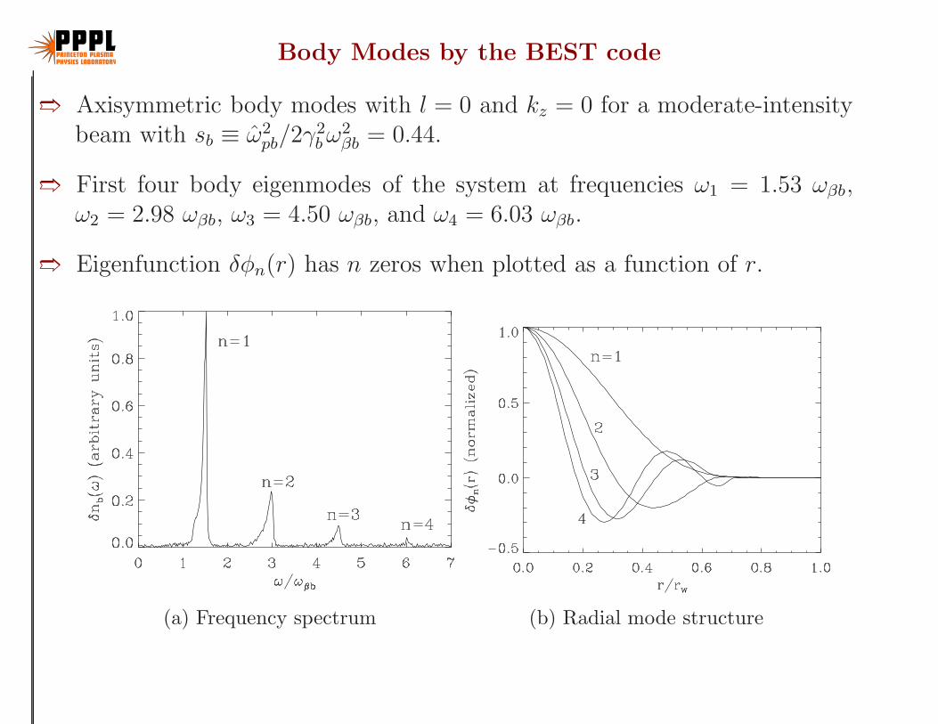
Body Modes by the BEST code

➱ Axisymmetric body modes with l = 0 and kz = 0 for a moderate-intensitybeam with sb ≡ ω2

pb/2γ2bω

2βb = 0.44.

➱ First four body eigenmodes of the system at frequencies ω1 = 1.53 ωβb,ω2 = 2.98 ωβb, ω3 = 4.50 ωβb, and ω4 = 6.03 ωβb.

➱ Eigenfunction δφn(r) has n zeros when plotted as a function of r.

(a) Frequency spectrum (b) Radial mode structure

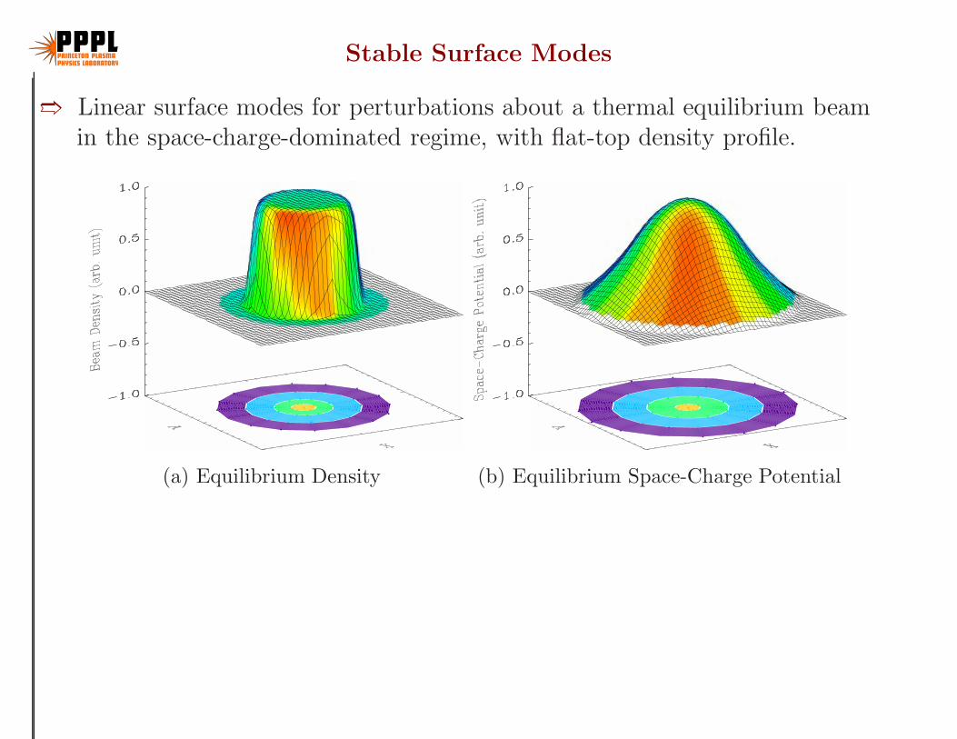
Stable Surface Modes

➱ Linear surface modes for perturbations about a thermal equilibrium beamin the space-charge-dominated regime, with flat-top density profile.

(a) Equilibrium Density (b) Equilibrium Space-Charge Potential

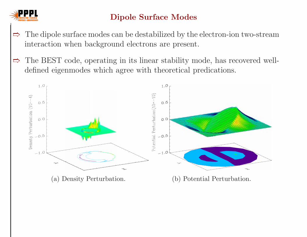
Dipole Surface Modes

➱ The dipole surface modes can be destabilized by the electron-ion two-streaminteraction when background electrons are present.

➱ The BEST code, operating in its linear stability mode, has recovered well-defined eigenmodes which agree with theoretical predications.

(a) Density Perturbation. (b) Potential Perturbation.

Dipole Surface Modes (l=1)

➱ For azimuthal mode number l = 1, the dispersion relation is given by

ω = kzVb ± ωpb√2γb

√1 − r2

b

r2w

(1)

where rb is the radius of the beam edge, and rw is location of the conductingwall. Here, ω2

pb = 4πnbe2b/γbmb is the ion plasma frequency-squared, and

ωpb/√

2γb w ωβb in the space-charge-dominated limit.

(a) ω/ωβb versus rw/rb (b) Spectrum for rw/rb = 2.2




❍➱ Collective two-stream interactions





Two-Stream Instability for Intense Ion Beams

➱ In the absence of background electrons, an intense nonneutral ion beamsupports collective oscillations (sideband oscillations) with phase velocityω/kz upshifted and downshifted relative to the average beam velocity βbc.

➱ Introduction of an (unwanted) electron component (produced, for example,by secondary emission of electrons due to the interaction of halo ions withthe chamber wall) provides the free energy to drive the classical two-streaminstability.

(OHFWURQ'LVWULEXWLRQ

%HDP,RQV

'RZQVKLIWHG 8SVKLIWHG

3KDVH�YHORFLW\ zκω/=

β bcβ ec

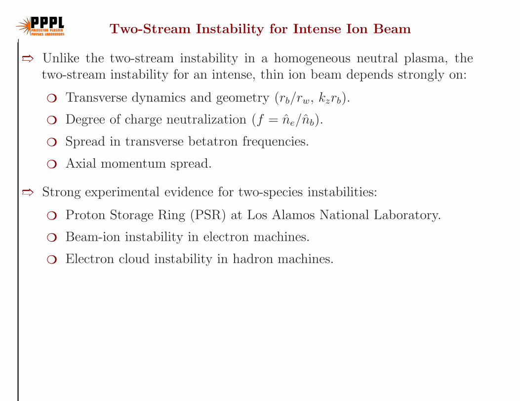
Two-Stream Instability for Intense Ion Beam

➱ Unlike the two-stream instability in a homogeneous neutral plasma, thetwo-stream instability for an intense, thin ion beam depends strongly on:

❍ Transverse dynamics and geometry (rb/rw, kzrb).

❍ Degree of charge neutralization (f = ne/nb).

❍ Spread in transverse betatron frequencies.

❍ Axial momentum spread.

➱ Strong experimental evidence for two-species instabilities:

❍ Proton Storage Ring (PSR) at Los Alamos National Laboratory.

❍ Beam-ion instability in electron machines.

❍ Electron cloud instability in hadron machines.

l = 1 Dipole Mode in a Moderate-Intensity Proton Beam

➱ Generally, these is no analytical description of the eigenmodes in beamswith nonuniform density profiles.

➱ However, numerical result shows that eigenmode is localized in the regionwhere the density gradient is large.

(a) Equilibrium Density Profile (b) Mode Structure

Electron-Proton Two-Stream Instability

➱ When a background electron component is introduced with βe = Ve/c w 0,the l = 1 dipole mode can be destabilized for a certain range of axialwavenumber and a certain range of electron temperature Te.

(a) t = 0 (b) t = 200/ωβb

Growth Rate for Illustrative PSR Parameters

➱ Illustrative parameters in the Proton Storage Ring (PSR) experiment.

❍ Space-charge-induced tune shift: δν/ν0 ∼ −0.020, ω2pb/2γ

2bω

2βb = 0.079.

❍ Oscillation frequency (simulations): f ∼ 163MHz. Mode number atmaximum growth n = 55 ∼ 65.

❍ λb = 9.13 × 108cm−1, λe = 9.25 × 107cm−1, Tb⊥ = 4.41keV, Te⊥ =0.73keV, φ0(rw) − φ0(0) = −3.08 × 103Volts.

Growth Rate for Two-Stream Instability

➱ Maximum growth rate depends on the normalized beam density nb/nb0 andthe initial axial momentum spread.

0 0.5 1 1.5 2

. %0 33

. %0 46

. %0 59

ˆ / ˆb bn n0

/ . %b bp p 0 00=∆P P

0.0

1.0

2.0

3.0

4.0

5.0

6.0

(Im

)/

()

max

ωω βb

10

2−

➱ nb0 = 9.41 × 108cm−3, corresponding to an average current of 35A in theProton Storage Ring (PSR) experiment (ω2

pb/2γ2bω

2βb = 0.079).

➱ A larger longitudinal momentum spread induces stronger Landau damp-ing by parallel kinetic effects and therefore reduces the growth rate of theinstability.

➱ Higher beam intensity provides more free energy to drive a stronger insta-bility.

Instability Threshold

➱ Important damping mechanisms includes

❍ Longitudinal Landau damping by the beam ions.

❍ Stabilizing effects due to space-charge-induced tune spread.

➱ An instability threshold is observed in the simulations.

00

0.5

1

1.5

2

nn

bb0

ˆ/

ˆ

p pb b−10 3/ ( )∆

P P

1 2 3 4 5 6

f = 0 05.

0 08.

0 10.

0 15.

0 20.

0 25.

➱ Larger momentum spread and smaller fractional charge neutralization im-ply a higher density threshold for the instability to occur.

Long-Time Evolution of the e-p Instability

➱ Late-time nonlinear phase of e-p instability.

➱ Late-time nonlinear growth observed for system parameters above marginalstability.

➱ Simulations show two phases to the e-p instability.

Long-Time Evolution of the e-p Instability

➱ Late-time nonlinear phase of e-p instability at twice the beam intensity.

➱ Nonlinear growth to larger amplitudes occurs on faster time scale.

Conclusions

➱ A 3D multispecies nonlinear perturbative particle simulation method hasbeen developed to study two-stream instabilities in intense charged particlebeams described self-consistently by the Vlasov-Maxwell equations.

➱ Introducing a background component of electrons, the two-stream insta-bility is observed in the simulations. Several properties of this instabilityare investigated numerically, and are found to be in qualitative agreementwith theoretical predictions.

➱ The self-consistent simulations show that the instability has a dipole modestructure, and the growth rate is an increasing function of proton densityand fractional charge neutralization.

➱ The simulations show that an axial momentum spread and the space-chargeinduced tune spread provide effective stabilization mechanisms for the e-pinstability.





❍➱ Instability driven by temperature anisotropy (T⊥b � T‖b).




Instability Driven by Large Temperature Anisotropy

Objective:• Determine linear and nonlinear dynamics of intense beams with large

temperature anisotropy

Approach:• Develop an analytical model based on linearized Vlasov-Maxwell equations

to describe Harris-like instability in intense beams. Apply nonlinear f BEST code to determine linear and nonlinear dynamics.References:

• “Delta-f Simulation Studies of the Stability Properties of Intense Charged Particle Beams with Temperature Anisotropy,” E. A. Startsev, R. C. Davidson and H. Qin, Proceedings of the 2001 Particle Accelerator Conference, 3080 (2001).

).( ||bb TT >>⊥

δ

• “Nonlinear F Simulation Studies of Intense Charged Particle Beams with Large Temperature Anisotropy,” E. A. Startsev, R. C. Davidson and H. Qin, Phys. Plasmas 9, in press (2002).

δ

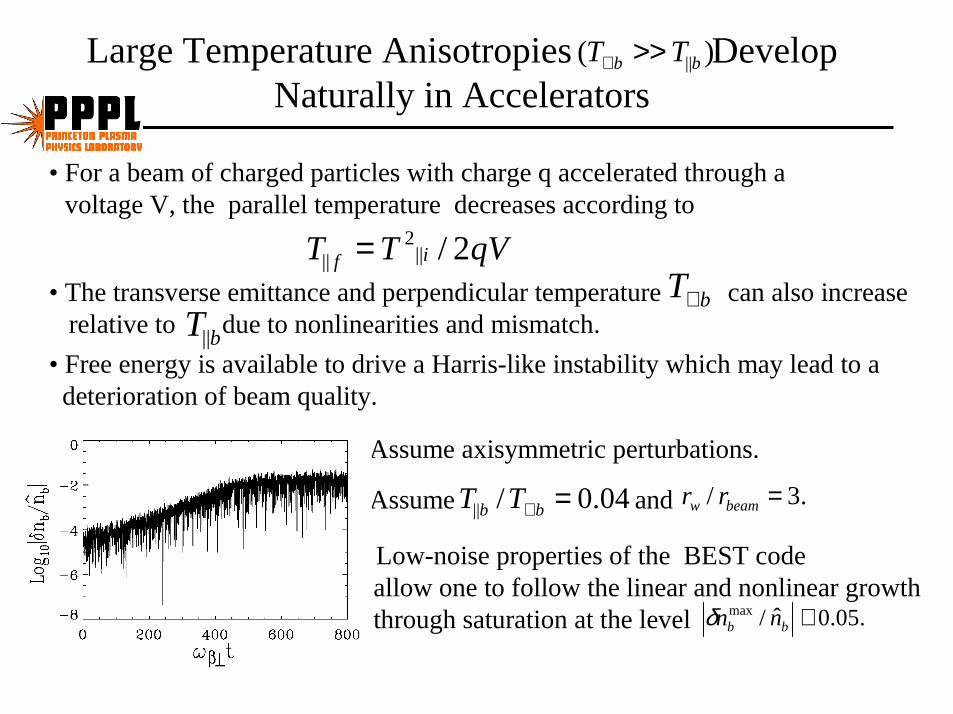
Large Temperature Anisotropies Develop Naturally in Accelerators

• For a beam of charged particles with charge q accelerated through a

• Free energy is available to drive a Harris-like instability which may lead to a deterioration of beam quality.

qVTT if 2/||2

|| =

)( ||bb TT >>⊥

• The transverse emittance and perpendicular temperature can also increase relative to due to nonlinearities and mismatch.

bT⊥

• Low-noise properties of the BEST codeallow one to follow the linear and nonlinear growththrough saturation at the level .05.0ˆ/max ≅bb nnδ

•Assume axisymmetric perturbations.

•Assume and04.0/|| =⊥ bb TT .3/ =beamw rr

bT||

voltage V, the parallel temperature decreases according to

Onset and Saturation of the Instability

• The formation of tails in the axial momentum distribution and the consequent saturation ofthe instability are attributed to resonant wave-particle interactions.

• Plot shows the net change in the longitudinalmomentum distribution where,ˆ/)( 0bzb FpFδ

,)( 32∫ ⊥= bzb fxdpdpF δδ .)2/(ˆˆ 2/1||

30 bbbbb TmnF πγ=

• The maximum growth rate occurs for with no instability in the region

038.0/)(Im max ≅⊥βωω,8.02/ˆ 222 ≅= ⊥βωγω bpbbs.5.0≤bs

•The instability is found to be absent if.07.0/|| >⊥ bb TT

Instability Threshold

• The instability is stabilized by formation of a tail in the longitudinal momentumdistribution and the consequent Landau damping of the wave excitations.

)0( || =bTγ• The growth rate for can be estimated as

,)/()0( 2/13|||| bbthbzb mTkT γγ ≅=

0|| =bT

• The final width of the longitudinal velocity distribution can be estimated as , where |v|v|| bph V−≅∆ ./v zph kω=

where thbT|| is the threshold temperature for

stabilization.






❍➱ Hamiltonian averaging techniques



Hamiltonian Averaging Techniques

Objective

➱ Develop a formalism based on the nonlinear Vlasov-Maxwell equations thatcan be used to investigate the equilibrium and stability properties of ageneral class of intense charged particle beam distributions propagatingthrough periodic focusing field configurations.

Approach

➱ Apply the third-order Hamiltonian averaging technique developed by Chan-nell [Phys. Plasmas 6, 982 (1999)] to the specific example of intense beampropagation through a periodic focusing quadrupole field.

Hamiltonian Averaging Techniques

References

➱ “Approximate Periodically-Focused Solutions to the Nonlinear Vlasov-MaxwellEquations for Intense Beam Propagation Through an Alternating-GradientField”, R. C. Davidson, H. Qin, and P. J. Channell, Physical Review SpecialTopics on Accelerators and Beams 2, 074401 (1999); 3, 029901 (2000).

➱ “Hamiltonian Formalism for Solving the Vlasov-Poisson Equations and itsApplication to Periodic Focusing Systems and the Coherent Beam-BeamInteractions”, S. I. Tzenov and R. C. Davidson, Physical Review SpecialTopics on Accelerators and Beams 5, 021001 (2002).

➱ ”Guiding-Center Vlasov-Maxwell Description of Intense Beam PropagationThrough a Periodic Focusing Field”, R. C. Davidson and H. Qin, PhysicalReview Special Topics on Accelerators and Beams 4, 104401 (2001).


➱ Consider a thin (rb � S) intense nonneutral ion beam (ion charge = +Zbe,rest mass = mb) propagating in the z-direction through a periodic focusingquadrupole field with average axial momentum γbmbβbc, and axial period-icity length S.

➱ Here, rb is the characteristic beam radius, Vb = βbc is the average axialvelocity, and (γb − 1)mbc

2 is the directed kinetic energy, where γb = (1 −β2

b )−1/2 is the relativistic mass factor.

➱ The particle motion in the beam frame is assumed to be nonrelativistic.


➱ Introduce the scaled ‘time’ variable

s = βbct

and the (dimensionless) transverse velocities

x′ =dx

dsand y′ =

dy

ds

➱ The beam particles propagate in the z-direction through an alternating-gradient quadrupole field

Bfocq (x) = B′

q(s)(yex + xey)

with lattice coupling coefficient defined by

κq(s) ≡ZbeB

′q(s)

γbmbβbc2

Here, B′q(s) ≡ (∂Bq

x/∂y)(0,0) = (∂Bqy/∂x)(0,0), and xex + yey is the trans-

verse displacement of a particle from the beam axis.

➱ Here,κq(s+ S) = κq(s)

where S = const. is the axial periodicity length.


➱ Neglecting the axial velocity spread, and approximating vz ' βbc, the ap-plied transverse focusing force on a beam particle is (inverse length units)

F foc = −κq(s)[xex − yey]

over the transverse dimensions of the beam (rb � S).

➱ The (dimensionless) self-field potential experienced by a beam ion is

ψ(x, y, s) =Zbe

γbmbβ2b c

2[φ(x, y, s) − βbAz(x, y, s)]

where φ(x, y, s) is the space-charge potential, and Az(x, y, s) ' βbφ(x, y, s)is the axial component of vector potential.

➱ The corresponding self-field force on a beam particle is (inverse lengthunits)

F self = −[∂ψ

∂xex +

∂ψ

∂yey

]


➱ Transverse particle orbits x(s) and y(s) in the laboratory frame are deter-mined from

d2

ds2x(s) + κq(s)x(s) = − ∂

∂xψ(x, y, s)

d2

ds2y(s) − κq(s)y(s) = − ∂

∂yψ(x, y, s)

➱ The characteristic axial wavelength λq of transverse particle oscillationsinduced by a quadrupole field with amplitude κq is

λq ∼ 2π√κq

➱ The dimensionless small parameter ε assumed in the present analysis s is

ε ∼(S

λq

)2

∼ κqS2

(2π)2< 1,

which is proportional to the strength of the applied focusing field.


➱ The laboratory-frame Hamiltonian H(x, y, x′, y′, s) for single-particle mo-tion in the transverse phase space (x, y, x′, y′) is

H(x, y, x′, y′, s) =1

2(x′2 + y′2)

+1

2κq(s)(x

2 − y2) + ψ(x, y, s)

➱ The Vlasov equation describing the nonlinear evolution of the distributionfunction fb(x, y, x

′, y′, s) in laboratory-frame variables is given by{∂

∂s+ x′

∂

∂x+ y′

∂

∂y−

(κq(s)x+

∂ψ

∂x

)∂

∂x′

−(−κq(s)y +

∂ψ

∂y

)∂

∂y′

}fb = 0,

where ψ(x, y, s) = ebφs(x, y, s)/γ3

bmbβ2b c

2 is the dimensionless self-field po-tential.


➱ The self-field potential ψ(x, y, s) is determined self-consistently in terms ofthe distribution function fb(x, y, x

′, y′, s) from(∂2

∂x2+

∂2

∂y2

)ψ = −2πKb

Nb

∫dx′dy′fb

➱ Here, nb(x, y, s) =∫dx′dy′fb(x, y, x

′, y′, s) is the number density of thebeam ions, and the constants, Kb and Nb, are the self-field perveance andthe number of beam ions per unit axial length, respectively, defined by

Kb =2NbZ

2b e

2

γ3bmbβ2

b c2

= const.

Nb =

∫dxdydx′dy′fb = const.

Canonical Transformation to Slow Variables

➱ Transform from laboratory-frame variables (x, y, x′, y′) to ‘slow’ variables(X,Y,X ′, Y ′) and new Hamiltonian H(X,Y,X ′, Y ′, s).

➱ Formalism employs a canonical transformation to transform away the rapidlyoscillating terms in the laboratory-frame Hamiltonian.

➱ Formally express the laboratory-frame Hamiltonian as

H(x, y, x′, y′, s) = εH(x, y, x′, y′, s)

= ε

[1

2(x′2 + y′2) + V (x, y, s) + ψ(x, y, s)

]

where ε is a small dimensionless parameter proportional to the focusingfield strength.

➱ Here, V (x, y, s) is the potential for the applied focusing field

V (x, y, s) =1

2κq(s)(x

2 − y2)

where∫ S

0dsκq(s) = 0.


➱ Introduce a near-identity canonical transformation where the expandedgenerating function is defined by

S(x, y,X ′, Y ′, s) = xX ′ + yY ′ +∞∑

n=1

εnSn(x, y,X ′, Y ′, s)

➱ The transformed Hamiltonian H(X,Y,X ′, Y ′, s) in the slow variables isgiven by

H(X,Y,X ′, Y ′, s) = H(x, y, x′, y′, s) +∂

∂sS(x, y,X ′, Y ′, s)

➱ Expressing H =∑∞

n=1 εnHn gives

∞∑n=1

εnHn(X,Y,X ′, Y ′, s)

= ε

[1

2(x′2 + y′2) + V (x, y, s) + ψ(x, y, s)

]

+

∞∑n=1

εn∂

∂sSn(x, y,X ′, Y ′, s)


➱ Solve for Sn(x, y,X ′, Y ′, s), order by order, enforcing the requirement thatthe transformed Hamiltonian H(X, Y , X ′, Y ′, s) be slowly varying.

➱ This gives (correct to order ε3 ) the slowly varying Hamiltonian

H(X, Y , X ′, Y ′, s) =1

2(X ′2 + Y ′2)

+1

2κf(X

2 + Y 2) + ψ(X, Y , s)

➱ Here, κf is the constant focusing coefficient defined by

κf ≡ κfq =1

S

∫ S

0

ds[α2q(s) − 〈αq〉2]

αq(s) =

∫ s

0

dsκq(s) , 〈αq〉 =1

S

∫ S

0

dsαq(s)

Transformed Hamiltonian andCoordinate Transformation

➱ The coordinate transformation relating the laboratory-frame variables (x, y, x′, y′)to the slow variables (X, Y , X ′, Y ′) is then given correct to order ε3 by

x(X, Y , X ′, Y ′, s) = [1 − βq(s)]X + 2

(∫ s

0

dsβq(s)

)X ′

y(X, Y , X ′, Y ′, s) = [1 + βq(s)]Y − 2

(∫ s

0

dsβq(s)

)Y ′

and

x′(X, Y , X ′, Y ′, s) = [1 + βq(s)]X′ + {−αq(s) + 〈αq〉〈αq〉βq(s) − αq(s)βq(s)

−(∫ s

0

ds[δq(s) − 〈δq〉])}X +

(∫ s

0

dsβq(s)

)∂

∂X

(X∂ψ

∂X− Y

∂ψ

∂Y

)

y′(X, Y , X ′, Y ′, s) = [1 − βq(s)]Y′ + {αq(s) − 〈αq〉 + 〈αq〉βq(s) − αq(s)βq(s)

−(∫ s

0

ds[δq(s) − 〈δq〉])}Y −

(∫ s

0

dsβq(s)

)∂

∂Y

(Y∂ψ

∂Y− X

∂ψ

∂X

)

Nonlinear Vlasov-Maxwell Equationsin the Transformed Variables

➱ For the transformed Hamiltonian, the single-particle equations of motionare given by

d

dsX =

∂H∂X

′ = X ′ex + Y ′ey

d

dsX

′= − ∂H

∂X= −κf(Xex + Y ey) − ∂

∂Xψ(X, Y , s)

➱ The nonlinear Vlasov equation for the distribution function Fb(X, Y , X′, Y ′, s)

in the transformed variables is then given by{∂

∂s+ X ′ ∂

∂Y+ Y ′ ∂

∂Y−

(κfX +

∂

∂Xψ

)∂

∂X ′

−(κf Y +

∂

∂Yψ

)∂

∂Y ′

}Fb(X, Y , X

′, Y ′, s) = 0


➱ The characteristics of the Vlasov equation correspond to the single-particleequations of motion in the applied-field plus self-field configuration.

➱ The slowly-varying self-field potential ψ(X, Y , s) is determined self-consistentlyin terms of the distribution function Fb(X, Y , X

′, Y ′, s) from

(∂2

∂X2+

∂2

∂Y 2

)ψ(X, Y , s)

= −2πKb

Nb

∫dX ′dY ′Fb(X, Y , X

′, Y ′, s)

➱ Because the coordinate transformation is canonical, the laboratory-framedistribution function fb(x, y, x

′, y′, s) is related to the transformed distribu-tion function Fb(X, Y , X

′, Y ′, s) by

fb(x, y, x′, y′, s)dxdydx′dy′ = Fb(X, Y , X

′, Y ′, s)dXdY dX ′dY ′


➱ The Jacobian of the transformation is equal to unity

∂(x, y, x′, y′)

∂(X, Y , X ′, Y ′)= 1

which can also be verified correct to order ε3 by direct calculation.

➱ Nonlinear Vlasov-Maxwell equations for Fb(X, Y , X′, Y ′, s) and ψ(X, Y , s)

in the slow variables (X, Y , X ′, Y ′) can be used to investigate detailed equi-librium and stability properties over a wide range of system parameters,including beam intensity [Kb] and choice of periodic lattice function [κq(s)].

➱ Because the focusing coefficient is constant (κf = const.) in the trans-formed variables, analysis of the nonlinear Vlasov-Maxwell equations forFb(X, Y , X

′, Y ′, s) and ψ(X, Y , s) is far more amenable to direct calcula-tion than the nonlinear Vlasov-Maxwell equations for fb(x, y, x

′, y′, s) andψ(x, y, s) in laboratory-frame variables.

➱ Because κf = const. in the transformed variables, a wide body of kineticequilibrium and stability literature derived in the constant-focusing casecan be applied virtually intact.


➱ Because the focusing force, F foc = −κf(Xex + Y ey), is isotropic in thetransverse plane, the nonlinear Vlasov-Maxwell equations for Fb(X, Y , X

′, Y ′, s)and ψ(X, Y , s) support a broad class of equilibrium solutions (∂/∂s = 0)which are axisymmetric (∂/∂Θ = 0) in the transformed variables.

➱ The corresponding solutions for fb(x, y, x′, y′, s) and ψ(x, y, s) in laboratory-

frame variables, however, are periodically focused with axial periodicitylength S = const.

➱ While the transformed variables (X, Y ) are ‘space-like’ and (X ′, Y ′) are‘velocity-like’, it is important to keep in mind that the dependence of(x, y, x′, y′) on (X, Y , X ′, Y ) is inexorably mixed by the coordinate trans-formation derived earlier.

Conclusions

➱ The present formalism represents a powerful framework for describing periodically-focused beam propagation through an alternating-gradient quadrupole fo-cusing field, κq(s+ S) = κq(s), at arbitrary beam intensity.

➱ Circular cross-section beam equilibria in the transformed variables (X, Y , X ′, Y ′),back-transform to periodically-focused pulsating beam distribution func-tions with elliptical cross-section in the laboratory-frame variables (x, y, x′, y′).

➱ Because κf = const. in the transformed variables, a large body of constant-focusing equilibrium and stability results can be applied virtually intact.

Conclusions

➱ One key result is the kinetic stability theorem, which demonstrates that(∂/∂H0)F 0

b (H0) ≤ 0 is a sufficient condition for stability (linear and non-linear).

➱ Within the context of the present analysis, there are numerous beam equi-libria F 0

b (H0) in the transformed variables (X, Y , X ′, Y ), with correspond-ing (periodically-focused) beam distributions in laboratory-frame variables(x, y, x′, y′).

➱ No longer is the Kapchinskij-Vladimirskij (KV) distribution the only knownperiodically-focused solution to the nonlinear Vlasov-Maxwell equations.







❍➱ Halo particle production by collective excitations


Halo Particle Production byCollective Excitations in Intense Beams

Background

➱ Frequently explored mechanisms for production of halo particles in in-tense beams include beam mismatch, envelope instabilities, and nonuniformcharge density, using test-particle and particle-core models as appropriate.

Recent Developement

➱ Collective wave excitations, even in a matched beam, provide an additionalmechanism for ejecting halo particles from the beam core.

References

➱ “Production of Halo Particles by Excitation of Collective Modes in High-Intensity Charged Particle Beams,” S. Strasburg and R. C. Davidson, Phys-ical Review E61, 5753 (2000).

➱ ”Warm-Fluid Collective Mode Excitations in Intense Charged Particle Beams– Test Particle Simulations”, S. Strasburg and R. C. Davidson, Nucl. Instr.and Meth. in Phys. Res. A464, 524 (2001).

Theoretical Model

➱ Assume collective oscillations about an intense axisymmetric beam (∂/∂θ =0) in the smooth-focusing approximation with applied focusing force

F foc = −γbmbω2βb(xex + yey).

➱ Assume matched-beam equilibrium (constant rms radius), and follow thetest-particle motion, including the combined effects of the applied focus-ing and equilibrium space-charge forces, and the self-consistent collectiveoscillations.

➱ Electrostatic potential is expressed as

φ(r, t) = φ(r) + δφ(r, t)

where the oscillating potential δφ is calculated self-consistently using thewarm-fluid model for perturbations about a step-function waterbag densityprofile (Lund and Davidson) or a waterbag density profile (Strasburg andDavidson).

Theoretical Model

➱ Defines ≡ βbct κf ≡ ω2

βb/β2b c

2

ψ(r, s) =qb

γ3bmbβ2

b c2φ(r, s).

➱ Radial orbit equation for a test particle is

d2r

ds2+

(κf +

1

r

∂ψ0

∂r+

1

r

∂δψ

∂r

)r =

P 2θ

r3,

➱ For a matched beam, and δψ = 0, the test particle motion is regular.

➱ For a matched beam, and δψ 6= 0, the nonlinear oscillatory force (−∂δψ/∂r)can induce chaotic particle motion, and eject particles from the beam core.

Poincare Plot: Low Beam Intensity

- 1.5 - 1.0 - 0.5 0.0 0.5 1.0 1.5

- 1.0

- 0.5

0.0

0.5

1.0

x

x’

(a) νν0

= 0.54, sb = 0.7, δnb

nb= 0

- 1.0 - 0.5 0.0 0.5 1.0

- 1.0

- 0.5

0.0

0.5

1.0

x

x’

x

(b) νν0

= 0.54, sb = 0.7, δnb

nb= 10%

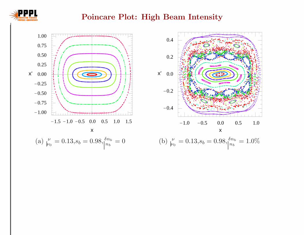
Poincare Plot: High Beam Intensity

- 1.5 - 1.0 - 0.5 0.0 0.5 1.0 1.5

- 1.00

- 0.75

- 0.50

- 0.25

0.00

0.25

0.50

0.75

1.00

x

x’

(a) νν0

= 0.13,sb = 0.98, δnb

nb= 0

- 1.0 - 0.5 0.0 0.5 1.0

- 0.4

- 0.2

0.0

0.2

0.4

x

x’

(b) νν0

= 0.13,sb = 0.98, δnb

nb= 1.0%

Poincare Plot: High Beam Intensity, Moderate ModeAmplitude

- 1.0 - 0.5 0.0 0.5 1.0

- 0.6

- 0.4

- 0.2

0.0

0.2

0.4

0.6

x

x’

System Parameters:

ν

ν0

= 0.13, sb = 0.98,δnb

nb

= 2.5%

Location of Resonances in Phase Space

0.2 0.4 0.6 0.80.00

0.50

0.75

1.00

1.25

1.50

2.00

υ/υ0

x

0.2 0.4 0.6 0.80.00

0.50

0.75

1.00

1.25

1.50

2.00

υ/υ0

x

n = 1, 2, 3, 4

For ν/ν0 = 0.54 with large amplitude perturbations, island chains arevisible (?) for 6:1, 13:2, 20:3, 7:1, and 8:1 resonances, and their locationsare very accurately predicted by analytic theory.








❍➱ Paul Trap Simulator Experiment

Objective:• Simulate collective processes and transverse dynamics of intense charged

particle beam propagation through an alternating-gradient quadrupole focusing field using a compact laboratory Paul trap.

Approach:• Investigate dynamics and collective processes in a long one-component charge

bunch confined in a Paul trap with oscillating wall voltage

References:• “A Paul Trap Configuration to Simulate Intense Nonneutral Beam Propagation Over Large Distances

Through a Periodic Focusing Quadrupole Magnetic Field,” R. C. Davidson, H. Qin, and G. Shvets, Physics of Plasmas 7, 1020 (2000).

• “Paul Trap Experiment for Simulating Intense Beam Propagation Through a Quadrupole Focusing Field,” R. C. Davidson, P. Efthimion, R. Majeski, and H. Qin, Proceedings of the 2001 Particle Accelerator Conference, 2978 (2001).

• “Paul Trap Simulator Experiment to Simulate Intense Beam Propagation Through a Periodic Focusing Quadrupole Field,” R. C. Davidson, P. C. Efthimion, E. Gilson, R. Majeski, and H. Qin, American Institute of Physics Conference Proceedings 606, 576 (2002).

).()( 00 tVTtV =+

Paul Trap Simulator Experiment

Paul Trap Simulator Configuration

(a) (b)

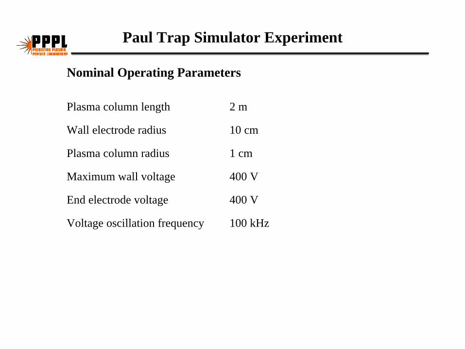
Nominal Operating Parameters

100 kHzVoltage oscillation frequency

400 VEnd electrode voltage

400 VMaximum wall voltage

1 cmPlasma column radius

10 cmWall electrode radius

2 mPlasma column length


),,())((21

)(21

),,,,( 2222 syxyxsyxsyxyxH q ψκ +−+′+′=′′⊥

223/),,(),,( ,/ ,/ where cmsyxesyxdsdyydsdxx bbbs

b βγφψ ==′=′

2

)()(

cm

sBes

bbb

qbq βγ

κ′

=

)()( sSs qq κκ =+

Transverse Hamiltonian (dimensionless units) for intense beam propagation through a periodic focusing quadrupole magnetic field is given by

and

with

Transverse Hamiltonian for IntenseBeam Propagation

),,(),,()(21

),,,,( 22 tyxetyxeyxsyxyxH sbapb φφ +++=⊥ &&&&

)2cos()2/sin()(4

),,(2

1

0 θπ

πφ l

ll

l

l

= ∑

∞

= wap r

rtVtyx

2022

)(8

)( where),)((21

),,(wb

bqqap rm

tVetyxttyx

πκκφ =−=

Transverse Hamiltonian for Particle Motionin a Paul Trap

Transverse Hamiltonian (dimensionless units) for a long charge bunch in a Paul trap with time periodic wall voltages bygiven is )()( 00 tVTtV =+

where the applied potential )0( wrr ≤≤

can be approximated by )for ( wp rr <<

Planned experimental studies include:

• Beam mismatch and envelope instabilities.

• Collective wave excitations.

• Chaotic particle dynamics and production of halo particles.

• Mechanisms for emittance growth.

• Effects of distribution function on stability properties.

Plasma is formed using a cesium source or a barium coated platinum or rhenium filament. Plasma microstate will be determined usinglaser-induced fluorescence (Levinton, FP&T).



Paul Trap Simulator Experiment vacuum chamber.

• Laboratory preparation, procurement, assembly, bakeout, and pumpdown of PTSX vacuum chamber to

2002). (May,Torr 1025.5 10−×


Paul Trap Simulator Experiment electrodes.

• Stainless steel gold-plated electrodes are supported by aluminum rings, teflon, and vespel spacers.


Paul Trap Simulator Experiment cesium source.

• Aluminosilicate cesium source produces up to 30 µA of ion current when a 200 V acceleration voltage is used.


Paul Trap Simulator Experiment Faraday cup.

• Faraday cup with sensitive electrometer allows 20 fC resolution. Linear motion feedthrough with 6" stroke allows measurement of radial density dependence.


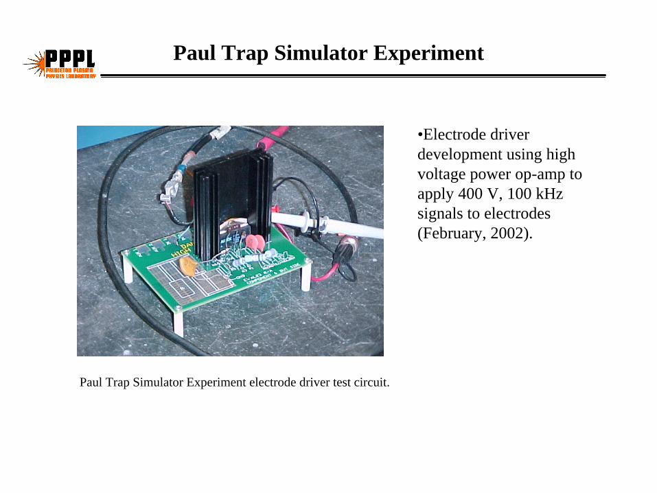
Paul Trap Simulator Experiment electrode driver test circuit.

•Electrode driver development using high voltage power op-amp to apply 400 V, 100 kHz signals to electrodes (February, 2002).

Paul Trap Simulator Experiment Initial Results

Current collected on Faraday cup versus radius.

• Experiment - stream Cs+

ions from source to collector without axial trapping of the plasma.

• V0(t) = V0 max sin (2π f t)• V0 max = 387.5 V• f = 90 kHz

• Vaccel = -183.3 V• Vdecel = -5.0 V

Ion source parameters:

Electrode parameters:

Conclusions

➱ Considerable progress has been made in developing and applying advancedtheoretical techniques and simulation capabilities based on the nonlinearVlasov-Maxwell equations to describe intense beam propagation.

➱ Quite remarkably, these capabilities can be applied over the entire range ofnormalized beam intensity

0 <ω2

pb

2γ2bω

2β⊥

< 1 .

➱ Advanced simulation studies benefit considerably from comparisons withanalytical results and experiment.

➱ Stay tuned for experimental results from the Paul Trap Simulator Experi-ment (PTSX).

ronald c. davidson intense self fieldphysics of charged … · · 2002-07-05ities based on...

Documents