root cause investigation best practices guide of objectivity/incorrect problem definition: the team...

AEROSPACE REPORT NO. TOR-2014-02202

Root Cause Investigation Best Practices Guide

May 30, 2014

Roland J. Duphily Acquisition Risk and Reliability Engineering Department Mission Assurance Subdivision

Prepared for: National Reconnaissance Office 14675 Lee Road Chantilly, VA 20151-1715

Contract No. FA8802-14-C-0001

Authorized by: National Systems Group

Developed in conjunction with Government and Industry contributions as part of the U.S. Space Program Mission Assurance Improvement Workshop.

Distribution Statement A: Approved for public release; distribution unlimited.

https://aeroreports.aero.org/faces/introduction.xhtml

https://aeroreports.aero.org/faces/introduction.xhtml

Report Documentation Page Form ApprovedOMB No. 0704-0188

Public reporting burden for the collection of information is estimated to average 1 hour per response, including the time for reviewing instructions, searching existing data sources, gathering andmaintaining the data needed, and completing and reviewing the collection of information. Send comments regarding this burden estimate or any other aspect of this collection of information,including suggestions for reducing this burden, to Washington Headquarters Services, Directorate for Information Operations and Reports, 1215 Jefferson Davis Highway, Suite 1204, ArlingtonVA 22202-4302. Respondents should be aware that notwithstanding any other provision of law, no person shall be subject to a penalty for failing to comply with a collection of information if itdoes not display a currently valid OMB control number.

1. REPORT DATE 30 MAY 2014

2. REPORT TYPE Final

3. DATES COVERED -

4. TITLE AND SUBTITLE Root Cause Investigation Best Practices Guide

5a. CONTRACT NUMBER FA8802-14-C-0001

5b. GRANT NUMBER

5c. PROGRAM ELEMENT NUMBER

6. AUTHOR(S) Roland J. Duphily

5d. PROJECT NUMBER

5e. TASK NUMBER

5f. WORK UNIT NUMBER

7. PERFORMING ORGANIZATION NAME(S) AND ADDRESS(ES) The Aerospace Corporation 2310 E. El Segundo Blvd. El Segundo, CA 90245-4609

8. PERFORMING ORGANIZATION REPORT NUMBER TOR-2014-02202

9. SPONSORING/MONITORING AGENCY NAME(S) AND ADDRESS(ES) National Reconnaissance Office 14675 Lee Road Chantilly, VA20151-1715

10. SPONSOR/MONITOR’S ACRONYM(S) NRO

11. SPONSOR/MONITOR’S REPORT NUMBER(S)

12. DISTRIBUTION/AVAILABILITY STATEMENT Approved for public release, distribution unlimited

13. SUPPLEMENTARY NOTES The original document contains color images.

14. ABSTRACT

15. SUBJECT TERMS

16. SECURITY CLASSIFICATION OF: 17. LIMITATIONOF ABSTRACT

UU

18. NUMBEROF PAGES

110

19a. NAME OFRESPONSIBLE PERSON

a. REPORT unclassified

b. ABSTRACT unclassified

c. THIS PAGE unclassified

Standard Form 298 (Rev. 8-98) Prescribed by ANSI Std Z39-18

i

Executive Summary

This guide has been prepared to help determine what methods and software tools are available when significant detailed root cause investigations are needed and what level of rigor is appropriate to reduce the likelihood of missing true root causes identification. For this report a root cause is the ultimate cause or causes that, if eliminated, would have prevented recurrence of the failure. In reality, many failures require only one or two investigators to identify root causes and do not demand an investigation plan that includes many of the practices defined in this document.

During ground testing and on-orbit operations of space systems, programs have experienced anomalies and failures where investigations did not truly establish definitive root causes. This has resulted in unidentified residual risk for future missions. Some reasons the team observed for missing the true root cause include the following:

1. Incorrect team composition: The lead investigator doesn’t understand how to perform an independent investigation and doesn’t have the right expertise on the team. Many times specialty representatives, such as parts, materials, and processes people are not part of the team from the beginning. (Sec 5.3)

2. Incorrect data classification: Investigation based on assumptions rather than objective evidence. Need to classify data accurately relative to observed facts (Sec 6.1)

3. Lack of objectivity/incorrect problem definition: The team begins the investigation with a likely root cause and looks for evidence to validate it, rather than collecting all of the pertinent data and coming to an objective root cause. The lead investigator may be biased toward a particular root cause and exerts their influence on the rest of the team members. (Sec 7)

4. Cost and schedule constraints: A limited investigation takes place in the interest of minimizing impacts to cost and schedule. Typically the limited investigation involves arriving at most likely root cause by examining test data and not attempting to replicate the failed condition. The actual root cause may lead to a redesign which becomes too painful to correct.

5. Rush to judgment: The investigation is closed before all potential causes are investigated. Only when the failure reoccurs is the original root cause questioned. “Jumping” to a probable cause is a major pitfall in root cause analysis (RCA).

6. Lack of management commitment: The lead investigator and team members are not given management backing to pursue root cause; quick closure is emphasized in the interest of program execution.

7. Lack of insight: Sometimes the team just doesn’t get the inspiration that leads to resolution. This can be after extensive investigation, but at some point there is just nothing else to do.

The investigation to determine root causes begins with containment, then continues with preservation of scene of failure, identifying an anomaly investigation lead, a preliminary investigation, an appropriate investigation team composition, failure definition, collection/analysis of data available before the failure, establishing a timeline of events, selecting the root cause analysis methods to use and any software tools to help the process.

This guide focuses on the early actions associated with the broader Root Cause Corrective Action (RCCA) process. The focus here includes the step beginning with the failure and ending with the root cause analysis step. It is also based on the RCI teams’ experience with space vehicle related failures

ii

on the ground as well as on-orbit operations. Although many of the methods discussed are applicable to ground and on-orbit failures, we discuss the additional challenges associated with on-orbit failures. Subsequent corrective action processes are not a part of this guide. Beginning with a confirmed significant anomaly we discuss the investigation team structure, what determines a good problem definition, several techniques available for the collection and classification of data, guidance for the anomaly investigation team on root cause analysis rigor needed, methods, software tools and also know when they have identified and confirmed the root cause or causes.

iii

Acknowledgments

Development of the Root Cause Investigation Best Practices Guide resulted from the efforts of the 2014 Mission Assurance Improvement Workshop (MAIW) Root Cause Investigation (RCI) topic team. Significant technical inputs, knowledge sharing, and disclosure were provided by all members of the team to leverage the industrial base to the maximum extent possible. For their content contributions, we thank the following contributing authors for making this collaborative effort possible:

Harold Harder (Co-Lead) The Boeing Company Roland Duphily (Co-Lead) The Aerospace Corporation Rodney Morehead The Aerospace Corporation Joe Haman Ball Aerospace & Technologies Corporation Helen Gjerde Lockheed Martin Corporation Susanne Dubois Northrop Grumman Corporation Thomas Stout Northrop Grumman Corporation David Ward Orbital Sciences Corporation Thomas Reinsel Raytheon Space and Airborne Systems Jim Loman SSL Eric Lau SSL

A special thank you goes to Harold Harder, The Boeing Company, for co-leading this team, and to Andrew King, The Boeing Company, for sponsoring this team. Your efforts to ensure the completeness and quality of this document are appreciated.

The Topic Team would like to acknowledge the contributions and feedback from the following subject matter experts who reviewed the document:

Lane Saechao Aerojet Rocketdyne Tom Hecht The Aerospace Corporation Matthew Eby The Aerospace Corporation David Eckhardt BAE Systems Gerald Schumann NASA Mark Wroth Northrop Grumman Corporation David Adcock Orbital Sciences Corporation Mauricio Tapia Orbital Sciences Corporation

iv

Release Notes

Although there are many failure investigation studies available, there is a smaller sample of ground related failure reports or on-orbit mishap reports where the implemented corrective action did not eliminate the problem and it occurred again. Our case study addresses a recurring failure where the true root causes were not identified during the first event.

v

Table of Contents

1. Overview ...................................................................................................................................... 1 1.1 MAIW RCI Team Formation ........................................................................................... 1

2. Purpose and Scope ........................................................................................................................ 2

3. Definitions .................................................................................................................................... 4

4. RCA Key Early Actions ............................................................................................................... 7 4.1 Preliminary Investigation .................................................................................................. 7 4.2 Scene Preservation and Data Collection ........................................................................... 8

4.2.1 Site Safety and Initial Data Collection ............................................................... 8 4.2.2 Witness Statements ............................................................................................ 9 4.2.3 Physical Control of Evidence ........................................................................... 10

4.3 Investigation Team Composition and Facilitation Techniques ....................................... 11 4.3.1 Team Composition ........................................................................................... 11 4.3.2 Team Facilitation Techniques .......................................................................... 12

5. Collect and Classify Data ........................................................................................................... 15 5.1 KNOT Chart ................................................................................................................... 17 5.2 Event Timeline ................................................................................................................ 17 5.3 Process Mapping ............................................................................................................. 18

6. Problem Definition ..................................................................................................................... 20

7. Root Cause Analysis (RCA) Methods ........................................................................................ 22 7.1 RCA Rigor Based on Significance of Anomaly ............................................................. 22 7.2 Brainstorming Potential Causes/Contributing Factors .................................................... 26 7.3 Fishbone Style ................................................................................................................ 26 7.4 Tree Techniques .............................................................................................................. 28

7.4.1 5-Why’s ............................................................................................................ 28 7.4.2 Cause Mapping ................................................................................................. 29 7.4.3 Advanced Cause and Effect Analysis (ACEA) ................................................ 30 7.4.4 Fault Tree Analysis (FTA) ............................................................................... 32

7.5 Process Flow Style .......................................................................................................... 34 7.5.1 Process Classification ....................................................................................... 34 7.5.2 Process Analysis ............................................................................................... 35

7.6 RCA Stacking ................................................................................................................. 36

8. Root Cause Analysis Tools (Software Package Survey) ............................................................ 38 8.1 Surveyed Candidates ...................................................................................................... 38 8.2 Reality Charting (Apollo) ............................................................................................... 39 8.3 TapRooT ......................................................................................................................... 40 8.4 GoldFire .......................................................................................................................... 43 8.5 RCAT (NASA Tool) ....................................................................................................... 45 8.6 Think Reliability ............................................................................................................. 47

9. When is RCA Depth Sufficient .................................................................................................. 49 9.1 Prioritization Techniques ................................................................................................ 51

9.1.1 Risk Cube ......................................................................................................... 51 9.1.2 Solution Evaluation Template .......................................................................... 52

10. RCA On-Orbit versus On-Ground .............................................................................................. 54

11. RCA Unverified and Unknown Cause Failures .......................................................................... 56

vi

11.1 Unverified Failure (UVF) ............................................................................................... 56 11.2 Unknown Direct/Root Cause Failure ............................................................................. 58

12. RCA Pitfalls ................................................................................................................................ 60

13. References ................................................................................................................................... 61

Appendix A. Case Study ............................................................................................................... A-1 A.1 Type B Reaction Wheel Root Cause Case Study ......................................................... A-1 A.2 Case Study – South Solar Array Deployment Anomaly .............................................. A-2

Appendix B. Data Collection Approaches ..................................................................................... B-1 B.1 Check Sheet .................................................................................................................. B-1 B.2 Control Charts .............................................................................................................. B-2 B.3 Histograms ................................................................................................................... B-4 B.4 Pareto Chart .................................................................................................................. B-7 B.5 Scatter Diagram ............................................................................................................ B-9 B.6 Stratification ............................................................................................................... B-15 B.7 Flowcharting............................................................................................................... B-17

Appendix C. Data Analysis Approaches ........................................................................................ C-1 C.1 Decision Matrix ............................................................................................................ C-1 C.2 Multi-voting ................................................................................................................. C-5

vii

Figures

Figure 1. Root cause investigation and RCCA. ........................................................................... 3 Figure 2. KNOT chart example. ................................................................................................ 17 Figure 3. Process mapping example. ......................................................................................... 19 Figure 4. Problem definition template. ...................................................................................... 21 Figure 5. Recommended methods for simple versus complex problems. ................................. 23 Figure 6. RCA rigor matrix. ...................................................................................................... 23 Figure 7. Example of RCA methods by RCA impact level matrix............................................ 24 Figure 8. Ishikawa diagram (fishbone) example........................................................................ 27 Figure 9. Five Why process example. ........................................................................................ 29 Figure 10. Cause mapping methodology example. ...................................................................... 30 Figure 11. Advance Cause and Effect Analysis (ACEA) process. .............................................. 31 Figure 12. Adding KNOT chart elements to Cause Tree. ............................................................ 32 Figure 13. Fault Tree Analysis (FTA) elements. ......................................................................... 33 Figure 14. Fault Tree example. .................................................................................................... 34 Figure 15. Example of process classification Cause and Effect (CE) diagram. .......................... 35 Figure 16. Process analysis method example. ............................................................................. 36 Figure 17. RCA stacking example. .............................................................................................. 37 Figure 18. Reality charting cause and effect continuum. ............................................................. 39 Figure 19. Reality charting cause and effect chart example. ....................................................... 40 Figure 20. TapRooT 7-step process. ............................................................................................ 41 Figure 21. TapRooT snap chart example. .................................................................................... 42 Figure 22. GoldFire cause effect chart. ........................................................................................ 44 Figure 23. RCAT introduction page. ........................................................................................... 45 Figure 24. Think reliability cause mapping steps. ....................................................................... 47 Figure 25. Reading a cause map. ................................................................................................. 48 Figure 26. Example – sinking of the Titanic cause map. ............................................................. 48 Figure 27 . Root cause prioritization risk cube. ............................................................................ 52 Figure 28. Solution evaluation template. ..................................................................................... 53 Figure 30. Check sheet example. ............................................................................................... B-1 Figure 31. Out-of-control signals............................................................................................... B-4 Figure 32. Normal distribution. ................................................................................................. B-5 Figure 33. Right-skewed distribution ........................................................................................ B-5 Figure 34. Bimodal (double-peaked) distribution. ..................................................................... B-6 Figure 35. Plateau distribution. .................................................................................................. B-6 Figure 36. Edge peak distribution. ............................................................................................. B-6 Figure 37. Truncated or heart-cut distribution. .......................................................................... B-7 Figure 38. Customer complaints pareto. .................................................................................... B-8 Figure 39. Document complaints pareto. ................................................................................... B-9 Figure 40. Examples of where scatter diagrams are used. ......................................................... B-9 Figure 41. Points on scatter diagram. ...................................................................................... B-10 Figure 42. Scatter affected by several causes. ......................................................................... B-11 Figure 43. Degrees of correlation. ........................................................................................... B-12 Figure 44. Types of correlation. .............................................................................................. B-13 Figure 45. Distribution of points across scatter diagram. ........................................................ B-14 Figure 46. Purity vs iron stratification diagram. ...................................................................... B-16 Figure 47. High-level flowchart for an order-filling process. .................................................. B-18 Figure 48. Detailed flow chart example – filling an order. ...................................................... B-19 Figure 49. Decision matrix example. ......................................................................................... C-2 Figure 50. Multi-voting example. .............................................................................................. C-6

viii

Tables

Table 1. Root Cause Investigation Core Team Composition ...................................................... 1 Table 2. Common RCI Terminology .......................................................................................... 4 Table 3. Levels of Causation and Associated Actions ................................................................ 6 Table 4. Core Team Members Roles and Responsibilities ....................................................... 11 Table 5. Additional Team Members’ Roles and Responsibilities ............................................. 12 Table 6. Data Collection and Classification Tools ................................................................... 16 Table 7. WIRE Spacecraft Avionics Timeline for Cover Deployment .................................... 18 Table 8. RCA Methods Pros and Cons ..................................................................................... 25 Table 9. RCA Software Tools Surveyed ................................................................................... 38 Table 10. UVF Risk Assessment Process Example .................................................................... 57 Table 11. UVF Verification Checklist ........................................................................................ 57

1

1. Overview

A multi-discipline team composed of representatives from different organizations in national security space has developed the following industry best practices guidance document for conducting consistent and successful root cause investigations. The desired outcome of a successful root cause investigation process is the conclusive determination of root causes, contributing factors and undesirable conditions. This provides the necessary information to define corrective actions that can be implemented to prevent recurrence of the associated failure or anomaly. This guide also addresses the realities of complex system failures and technical and programmatic constraints in the event root causes are not determined.

The analysis to determine root causes begins with a single engineer for most problems. For more complex problems, identify an anomaly investigation lead/team and develop a plan to collect and analyze data available before the failure, properly define the problem, establish a timeline of events, select the root cause analysis methods to use along with any software tools to help the process.

This guide focuses on specific early actions associated with the broader Root Cause Corrective Action (RCCA) process. The focus is the early root cause investigation steps of the RCCA process associated with space system anomalies during ground testing and on-orbit operations that significantly impact the RCA step of the RCCA process. Starting with a confirmed significant anomaly we discuss the collection and classification of data, what determines a good problem definition and what helps the anomaly investigation team select methods and software tools and also know when they have identified and confirmed the root cause or causes.

1.1 MAIW RCI Team Formation

The MAIW steering committee identified representatives from each of the participating industry partners as shown in Table 1. Weekly telecons and periodic face-to-face meetings were convened to share experiences between contractors and develop the final product.

Table 1. Root Cause Investigation Core Team Composition

The Aerospace Corporation Roland Duphily, Rodney Morehead Ball Aerospace and Technologies Corporation Joe Haman The Boeing Company Harold Harder Lockheed Martin Corporation Helen Gjerde Northrop Grumman Corporation Susanne Dubois, Thomas Stout Orbital Sciences Corporation David Ward Raytheon Space and Airborne Systems Thomas Reinsel SSL Jim Loman, Eric Lau

2

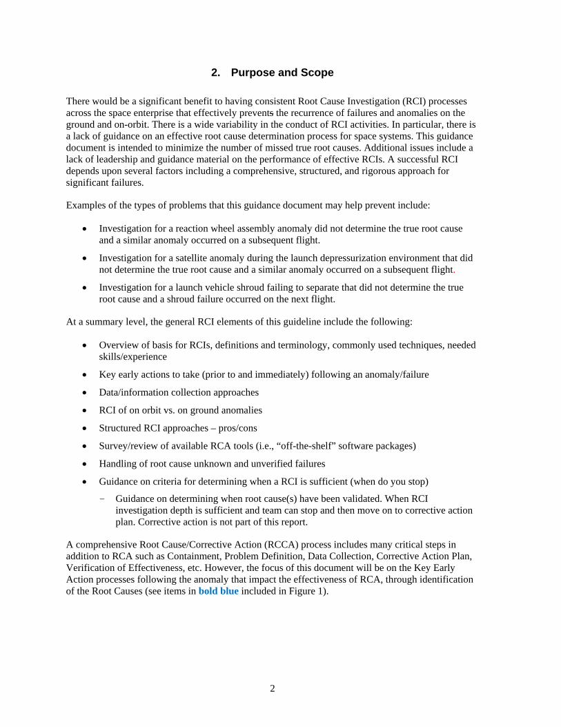
2. Purpose and Scope

There would be a significant benefit to having consistent Root Cause Investigation (RCI) processes across the space enterprise that effectively prevents the recurrence of failures and anomalies on the ground and on-orbit. There is a wide variability in the conduct of RCI activities. In particular, there is a lack of guidance on an effective root cause determination process for space systems. This guidance document is intended to minimize the number of missed true root causes. Additional issues include a lack of leadership and guidance material on the performance of effective RCIs. A successful RCI depends upon several factors including a comprehensive, structured, and rigorous approach for significant failures.

Examples of the types of problems that this guidance document may help prevent include:

• Investigation for a reaction wheel assembly anomaly did not determine the true root cause and a similar anomaly occurred on a subsequent flight.

• Investigation for a satellite anomaly during the launch depressurization environment that did not determine the true root cause and a similar anomaly occurred on a subsequent flight.

• Investigation for a launch vehicle shroud failing to separate that did not determine the true root cause and a shroud failure occurred on the next flight.

At a summary level, the general RCI elements of this guideline include the following:

• Overview of basis for RCIs, definitions and terminology, commonly used techniques, needed skills/experience

• Key early actions to take (prior to and immediately) following an anomaly/failure

• Data/information collection approaches

• RCI of on orbit vs. on ground anomalies

• Structured RCI approaches – pros/cons

• Survey/review of available RCA tools (i.e., “off-the-shelf” software packages)

• Handling of root cause unknown and unverified failures

• Guidance on criteria for determining when a RCI is sufficient (when do you stop)

- Guidance on determining when root cause(s) have been validated. When RCI investigation depth is sufficient and team can stop and then move on to corrective action plan. Corrective action is not part of this report.

A comprehensive Root Cause/Corrective Action (RCCA) process includes many critical steps in addition to RCA such as Containment, Problem Definition, Data Collection, Corrective Action Plan, Verification of Effectiveness, etc. However, the focus of this document will be on the Key Early Action processes following the anomaly that impact the effectiveness of RCA, through identification of the Root Causes (see items in bold blue included in Figure 1).

3

Figure 1. Root cause investigation and RCCA.

The remaining portions of the RCCA process either have either been addressed in previous MAIW documents (FRB Ref 1), or may be addressed in future MAIW documents.

Techniques employed to determine true root causes are varied, but this document identifies those structured approaches that have proven to be more effective than others. We discuss direct cause, immediate cause, proximate cause, and probable cause which are not true root causes. This document evaluates both creative “right-brain” activities such as brainstorming, as well as logical “left-brain” activities such as fault tree analyses, and will discuss the importance of approaching problems from different perspectives. The logical RCA methods include techniques such as Event Timeline, Fishbone Cause and Effect Diagram, Process Mapping, Cause and Effect Fault/Failure Tree, and RCA Stacking which combines multiple techniques. Several off-the-shelf software tools known by the team are summarized with vendor website addresses.

This document provides guidance on when to stop root cause identification process (validation of root causes), discusses special considerations for “on-orbit” vs. “on-ground” situations and how to handle “unverified” failures and “unknown” causes. In addition, a case study where the true root cause is missed, along with contributing factors is included in this document.

Finally, it is important to emphasize that trained and qualified individuals in RCCA facilitation, methods, tools and processes need to be present in, or available to, the organization.

4

3. Definitions

A common lexicon facilitates standardization and adoption of any new process. Table 2 defines terms used by the industry to implement the Failure Review Board (FRB) process. However, the authors note that significant variability exists even among the MAIW-participant contractors regarding terminology. Where this has occurred, emphasis is on inclusiveness and flexibility as opposed to historical accuracy or otherwise rigorous definitions.

Some of the more commonly used terms in RCI are shown in Table 2 below:

Table 2. Common RCI Terminology

Term Definition Acceptance Test A sequence of tests conducted to demonstrate workmanship and

provide screening of workmanship defects. Anomaly An unplanned, unexplained, unexpected, or uncharacteristic condition or

result or any condition that deviates from expectations. Failures, non-conformances, limit violations, out-of-family performance, undesired trends, unexpected results, procedural errors, improper test configurations, mishandling, and mishaps are all types of anomalies.

Component A stand-alone configuration item, which is typically an element of a larger subsystem or system. A component typically consists of built-up sub assemblies and individual piece parts.

Containment Appropriate, immediate actions taken to reduce the likelihood of additional system or component damage or to preclude the spreading of damage to other components. Containment may also infer steps taken to avoid creating an unverified failure or to avoid losing data essential to a failure investigation. In higher volume manufacturing containment may refer to quarantining and repairing as necessary all potentially effected materials.

Contributing Cause A factor that by itself does not cause a failure. In some cases, a failure cannot occur without the contributing cause (e.g., multiple contributing causes); in other cases, the contributing cause makes the failure more likely (e.g., a contributing cause and root cause).

Corrective Action An action that eliminates, mitigates, or prevents the root cause or contributing causes of a failure. A corrective action may or may not involve the remedial actions to the unit under test that bring it into conformance with the specification (or other accepted standard). However, after implementing the corrective actions, the design, the manufacturing processes, or test processes have changed so that they no longer lead to this failure on this type of UUT.

Corrective Action Process A generic closed-loop process that implements and verifies the remedial actions addressing the direct causes of a failure, the more general corrective actions that prevent recurrence of the failure, and any preventive actions identified during the investigation.

Destructive Physical Analysis (DPA)

Destructive Physical Analysis verifies and documents the quality of a device by disassembling, testing, and inspecting it to create a profile to determine how well a device conforms to design and process requirements.

Direct Cause (often referred to as immediate cause )

The event or condition that makes the test failure inevitable i.e., the event or condition event which is closest to, or immediately responsible for causing the failure. The condition can be physical (e.g., a bad solder joint) or technical (e.g., a design flaw), but a direct cause has a more fundamental basis for existence, namely the root cause. Some investigations reveal several layers of direct causes before the root cause, i.e., the real or true cause of the failure, becomes apparent. Also called proximate cause.

http://en.wikipedia.org/wiki/Causing

5

Term Definition Event Event is an unexpected behavior or functioning of hardware or software

which does not violate specified requirements and does not overstress or harm the hardware.

Failure A state or condition that occurs during test or pre-operations that indicates a system or component element has failed to meet its requirements.

Failure Modes and Effects Analysis (FMEA)

An analysis process which reviews the potential failure modes of an item and determines it effects on the item, adjacent elements, and the system itself.

Failure Review Board (FRB) Within the context of this guideline, a group, led by senior personnel, with authority to formally review and direct the course of a root-cause investigation and the associated actions that address the failed system.

Nonconformance The identification of the inability to meet physical or functional requirements as determined by test or inspection on a deliverable product.

Overstress An unintended event during test, integration, or manufacturing activities that result in a permanent degradation of the performance or reliability of acceptance, proto-qualification, or qualification hardware brought about by subjecting the hardware to conditions outside its specification operating or survival limits. The most common types of overstress are electrical, mechanical, and thermal.

Preventive Action An action that would prevent a failure that has not yet occurred. Implementations of preventive actions frequently require changes to enterprise standards or governance directives. Preventive actions can be thought of as actions taken to address a failure before it occurs in the same way that corrective actions systematically address a failure after it occurs.

Probable Cause A cause identified, with high probability, as the root cause of a failure but lacking in certain elements of absolute proof and supporting evidence. Probable causes may be lacking in additional engineering analysis, test, or data to support their reclassification as root cause and often require elements of speculative logic or judgment to explain the failure.

Proximate Cause The event that occurred, including any condition(s) that existed immediately before the undesired outcome, directly resulted in its occurrence and, if eliminated or modified, would have prevented the undesired outcome. Also called direct cause.

Qualification A sequence of tests, analyses, and inspections conducted to demonstrate satisfaction of design requirements including margin and product robustness for designs. Reference MIL-STD-1540 definitions

Remedial action An action performed to eliminate or correct a nonconformance without addressing the root cause(s). Remedial actions bring the UUT into conformance with a specification or other accepted standard. However, designing an identical UUT, or subjecting it to the same manufacturing and test flow may lead to the same failure. Remedial action is sometimes referred to as a correction or immediate action.

Root Cause The ultimate cause or causes that, if eliminated, would have prevented the occurrence of the failure.

Root-Cause Analysis (RCA) A systematic investigation that reviews available empirical and analytical evidence with the goal of definitively identifying a root cause for a failure.

Root Cause Corrective Action (RCCA) Combined activities of root cause analysis and corrective action.

Unit Under Test (UUT) The item being tested whose anomalous test results may initiate an FRB.

Unknown Cause A failure where the direct cause or root cause has not been determined. Unknown Direct Cause A repeatable/verifiable failure condition of unknown direct cause that

cannot be isolated to either the UUT or test equipment. Unknown Root Cause A failure that is sufficiently repeatable (verifiable) to be isolated to the

UUT or the test equipment, but whose root cause cannot be determined for any number of reasons.

6

Term Definition Unverified Failure (UVF) A failure (hardware, software, firmware, etc.) in the UUT or ambiguity

such that failure can’t be isolated to the UUT or test equipment. Transient symptoms usually contribute to the inability to isolate a UVF to direct cause. Typically a UVF does not repeat itself, preventing verification. Note that UVFs do not include failures that are in the test equipment once they have been successfully isolated there. UVFs have the possibility of affecting the flight unit after launch, and are the subject of greater scrutiny by the FRB.

Worst Case Analysis A circuit performance assessment under worst case conditions. It is used to demonstrate that it performs within specification despite particular variations in its constituent part parameters and the imposed environment, at the end of life (EOL).

Worst-Case Change Out (WCCO) (or Worst Case Rework/Repair)

An anomaly mitigation approach performed when the exact cause of the anomaly cannot be determined. The approach consists of performing an analysis to determine what system(s) or component(s) might have caused the failure and the suspect system(s) or component(s) are then replaced.

Table 3 reviews the terms “Remedial action,” “Corrective Action,” and “Preventive Action” for three levels of causation as follows:

Table 3. Levels of Causation and Associated Actions

Level of Causation (in order of increasing scope)

Action Taken to Mitigate Cause Scope of Action Taken

Direct Cause Remedial Action Addresses the specific nonconformance Root Cause Corrective Action Prevents nonconformance from recurring on

the program and/or other programs Potential Failure Preventive Action Prevents nonconformance from initially

occurring

7

4. RCA Key Early Actions

4.1 Preliminary Investigation

The first action that should be taken following a failure or anomaly is to contain the problem so that it does not spread or cause a personnel safety hazard, security issue, minimize impact to hardware, products, processes, assets, etc. Immediate steps should also be taken to preserve the scene of the failure until physical and/or other data has been collected from the immediate area and/or equipment involved before the scene becomes compromised and evidence of the failure is lost or distorted during the passage of time. It is during this very early stage of the RCCA process that we must collect, document and preserve facts, data, information, objective evidence, qualitative data (such as chart recordings, equipment settings/measurements etc.), and should also begin interviewing personnel involved or nearby. This data will later be classified using a KNOT Chart or similar tool. It is also critical to communicate as required to leadership and customers, and document the situation in as much detail as possible for future reference.

During the preliminary investigation, personnel should carefully consider the implications of the perceived anomaly. If executed properly, this element continues to safe the unit under test (UUT) and will preserve forensic evidence to facilitate the course of a subsequent root-cause investigation. In the event the nature of the failure precludes this (e.g., a catastrophic test failure), immediate recovery plans should be made. Some examples of seemingly benign actions that can be “destructive” if proper precautions are not taken for preserving forensic evidence include loosening fasteners without first verifying proper torque (once loosened, you’ll never know if it was properly tight); demating a connector without first verifying a proper mate; neglecting to place a white piece of paper below a connector during a demate to capture any foreign objects or debris.

Any preliminary investigation activities subsequent to the initial ruling about the necessity of an FRB are performed under the direction of the FRB chairperson or designee. The first investigative steps should attempt non-invasive troubleshooting activities such as UUT and test-set visual inspections and data reviews. Photographing the system or component and test setup to document the existing test condition or configuration is often appropriate. The photographs will help explain and demonstrate the failure to the FRB. The investigative team should record all relevant observables including the date and time of the failures (including overstress events), test type, test setup and fixtures, test conditions, and personnel conducting the test. The investigative team then evaluates the information collected, plans a course of action for the next steps of the failure investigation, and presents this information at a formal FRB meeting. Noninvasive troubleshooting should not be dismissed as a compulsory, low value exercise. There are a broad range of “best practices” that should be considered and adopted during the preliminary investigation process. The preliminary investigation process can be broken down into the following sub-phases:

• Additional safeguarding activities and data preservation

• Configuration containment controls and responsibilities

• Failure investigation plan and responsibilities

8

• Initial troubleshooting, data collection, and failure analysis (prior to breaking configuration) including failure timeline and primary factual data set related to failure event.

The actions of the preliminary investigation lead/team should be to verify that the immediate safe guarding actions taken earlier were done adequately. This includes verification of the initial assessment of damage and hardware conditions. This should also include the verification of data systems’ integrity and collected data prior to, and immediately after, the failure event occurrence. Once the area and systems are judged secure, additional considerations should be given to collecting initial photographic/video evidence and key eyewitness accounts (i.e., documented interviews). When the immediate actions are completed, securing the systems and the test area from further disturbance finalizes these actions.

Immediately following the safe-guarding and data-preservation actions, the preliminary investigation team, with help from the FRB and/or the program, should establish: area-access limitations, initial investigation constraints, and configuration-containment controls. The organization responsible for this should be involved in any further investigation requirements that could compromise evidence that may support the investigation. While this is often assigned to the quality or safety organizations it may vary across different companies and government organizations.

For Pre-Flight Anomalies, astute test design has been shown to improve the success of root cause investigations for difficult anomalies because of the following:

1. The test is designed to preserve the failure configuration; automatic test sets must stop on failure, rather than continuing on, giving more commands and even reconfiguring hardware.

2. Clever test design minimizes the chance of true unverified failures (UVFs) and ambiguous test results for both pre-flight and on-orbit anomalies;

3. The amount of clues available for the team is determined by what is chosen for telemetry or measured before the anomaly occurs.

4.2 Scene Preservation and Data Collection

4.2.1 Site Safety and Initial Data Collection

The cognizant authority, with support from all involved parties, should take immediate action to ensure the immediate safety of personnel and property. The scene should be secured to preserve evidence to the fullest extent possible. Any necessary activities that disturb the scene should be documented. Adapt the following steps as necessary to address the mishap location; on-orbit, air, ground, or water.

When the safety of personnel and property is assured, the first step in preservation is documentation. It may be helpful to use the following themes: Who, What, When, Where, and Environment. The next “W” is usually “Why” including “How,” but they are intentionally omitted since the RCCA process will answer those questions.

9

Consider the following as a start:

Who

• Who is involved and/or present? What was their role and location?

• What organization(s) were present? To what extent were they involved?

• Are there witnesses? All parties present should be considered witnesses, not just performers and management (e.g., security guard, IT specialist, etc.).

• Who was on the previous shift? Were there any indications of concern during recent shifts?

What

• What happened (without the why)? What is the sequence of events?

• What hardware, software, and/or processes were in use

• What operation being performed/procedure(s) in use? Occurred during normal or special conditions?

• What were the settings or modes on all relevant hardware and software?

When

• What is the time line? Match the timeline to the sequence of events.

Where

• Specific location of event

• Responsible individual(s) present

• Location of people during event (including shortly before as required)

Environment

• Pressure, temperature, humidity, lighting, radiation, etc.

• Hardware configurations (SV) and working space dimensions

• Working conditions including operations tempo, human factors, and crew rest

4.2.2 Witness Statements

It is often expected that personnel will provide a written statement after a mishap or anomaly. This is to capture as many of the details as possible while it is still fresh in the mind. The effectiveness of the subsequent RCA will be reduced if personnel believe their statements will be used against them in the future. There should be a policy and procedure governing the use of witness statements.

All statements should be obtained within the first 24 hours of the occurrence.

10

4.2.3 Physical Control of Evidence

The cognizant authority, with support from all involved parties, should control or impound if necessary all relevant data, documents, hardware, and sites that may be relevant to the subsequent investigation. Security should be set to control access to all relevant items until formally released by the cognizant authority.

Examples of data and documents include, but are not limited to:

• Drawings

• Check-out logs

• Test and check-out record charts

• Launch records

• Weather information

• Telemetry tapes

• Video tapes

• Audio tapes

• Time cards

• Training records

• Work authorization documents

• Maintenance and inspection records

• Problem reports

• Notes

• E-mail messages

• Automated log keeping systems

• Visitor’s logs

• Procedures

• The collection of observed measurements.

In addition, the acquisition of telemetry data over and above “tapes” should include telemetry from test equipment (if appropriate), and validating the time correlation between different telemetry streams (e.g., the time offset between the UUT telemetry and the test equipment telemetry).

11

4.3 Investigation Team Composition and Facilitation Techniques

4.3.1 Team Composition

The investigation team is multidisciplinary and may include members from Reliability, Product Line, Systems/Payload Engineering, Mission Assurance, On-Orbit Programs (for on-orbit investigations) and Failure Review Board. Additional team members may be assigned to ensure that subject matter experts (SMEs) are included, depending on the particular needs of each investigation.

The investigation team members are selected by senior leadership and/or mission assurance. Chair selection is critical to the success of the root cause analysis investigation. The ideal candidate is a person with prior experience in leading root cause investigations, has technical credibility, and has demonstrated the ability to bring a diverse group of people to closure on a technical issue. The root cause chair must be given the authority to operate independently of program management for root cause identification, but held accountable for appointing and completing task assignments. This is ideally a person who actively listens to the investigation team members’ points of view, adopts a questioning attitude, and has the ability to communicate well with the team members and program management. Above all the person must be able to objectively evaluate data and guide the team members to an understanding of the failure mechanism or scenario. The investigation team will be charged with completion of a final summary report and most likely an out-briefing presentation. If other priorities interfere with performing investigation responsibilities in a timely manner, it is their responsibility to address this with their management and report the issue and resolution to the investigation chairperson. At the discretion of the investigation chair, the investigation team membership may be modified during the course of the FRB depending on the resource needs of the investigation and personalities who may derail the investigation process. Table 4 identifies the core team member’s roles and responsibilities. Note one member may perform multiple responsibilities.

Table 4. Core Team Members Roles and Responsibilities

Core Team Member Roles and Responsibilities Investigation Chair Responsible for leading the investigation. Responsibilities include developing the

framework, managing resources, leading the root cause analysis process, identifying corrective actions, and creating the final investigation summary report.

Investigation Communications Lead (POC)

Responsible for internal and external briefings, status updates and general communications.

Mission Assurance Representative

Responsible for ensuring that the root cause is identified in a timely manner and corrective actions are implemented to address the design, performance, reliability and quality integrity of the hardware to meet customer requirements and flightworthiness standards.

Technical Lead Provides technical expertise and knowledge for all technical aspects of the hardware and/or processes under investigation.

Process Performers Know the actual/unwritten process and details.

Systems Lead Provides system application expertise and knowledge for all technical aspects of the spacecraft system under investigation.

12

Core Team Member Roles and Responsibilities Investigation Process Lead

Provides expertise and knowledge for the overall investigation process. Provides administration and analysis tools and ensures process compliance.

On-orbit program representative

Serves as a liaison between on-orbit program customer and Investigation team for on-orbit investigations.

Facilitator Provides guidance and keeps RCI team members on track when they meet (see 5.3.2).

Additional team members, as required:

Table 5 identifies the additional team members’ roles and responsibilities, qualifications required and functional areas of responsibility. Additional members are frequently specific “subject matter experts (SMEs)” needed to support the investigation.

Table 5. Additional Team Members’ Roles and Responsibilities

Additional team member Roles and Responsibilities

Product Lead Provides technical expertise and knowledge for the product and subassemblies under investigation.

Quality Lead Performs in-house and/or supplier Quality Engineering/Assurance activities during the investigation. Identifies and gathers the documentation pertinent to the hardware in question. Reviews all pertinent documentation to identify any anomalous condition that may be a contributor to the observed issue and provide the results to the Investigation.

Program Management Office (PMO) Representative

Responsible for program management activities during the investigation.

Customer Representative

Serves as a liaison between the investigation core team and the customer. Responsible for managing customer generated/assigned action items.

Subcontract Administrator

Responsible for conducting negotiations and maintaining effective working relationships and communications with suppliers on subcontract activities during the investigation (e.g., contractual requirements, action items, logistics).

Parts Engineering Responsible for parts engineering activities during the investigation, including searching pertinent screening and lot data, contacting the manufacturer, assessing the extent of the part contribution to the anomaly, analyzing the data.

Materials and Process (M&P) Engineering

Responsible for materials and process activities during the investigation, including searching pertinent lot data, contacting the manufacturer, assessing the extent of the material or process contribution to the anomaly and analyzing the data.

Failure Analysis Laboratory

Responsible for supporting failure analysis activities during the investigation.

Space Environments Responsible for space environment activities during the investigation. Reliability Analysis Responsible for design reliability analysis activities during the investigation. Planner Responsible for hardware planning activities during the investigation.

4.3.2 Team Facilitation Techniques

Team facilitation is more of an art than a science, and requires significant experience in order to be effective and efficient. Included among those facilitation techniques that have proven effective are:

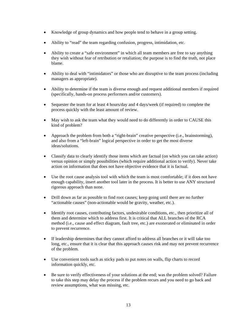
13

• Knowledge of group dynamics and how people tend to behave in a group setting.

• Ability to “read” the team regarding confusion, progress, intimidation, etc.

• Ability to create a “safe environment” in which all team members are free to say anything they wish without fear of retribution or retaliation; the purpose is to find the truth, not place blame.

• Ability to deal with “intimidators” or those who are disruptive to the team process (including managers as appropriate).

• Ability to determine if the team is diverse enough and request additional members if required (specifically, hands-on process performers and/or customers).

• Sequester the team for at least 4 hours/day and 4 days/week (if required) to complete the process quickly with the least amount of review.

• May wish to ask the team what they would need to do differently in order to CAUSE this kind of problem?

• Approach the problem from both a “right-brain” creative perspective (i.e., brainstorming), and also from a “left-brain” logical perspective in order to get the most diverse ideas/solutions.

• Classify data to clearly identify those items which are factual (on which you can take action) versus opinion or simply possibilities (which require additional action to verify). Never take action on information that does not have objective evidence that it is factual.

• Use the root cause analysis tool with which the team is most comfortable; if it does not have enough capability, insert another tool later in the process. It is better to use ANY structured rigorous approach than none.

• Drill down as far as possible to find root causes; keep going until there are no further “actionable causes” (non-actionable would be gravity, weather, etc.).

• Identify root causes, contributing factors, undesirable conditions, etc., then prioritize all of them and determine which to address first. It is critical that ALL branches of the RCA method (i.e., cause and effect diagram, fault tree, etc.) are exonerated or eliminated in order to prevent recurrence.

• If leadership determines that they cannot afford to address all branches or it will take too long, etc., ensure that it is clear that this approach causes risk and may not prevent recurrence of the problem.

• Use convenient tools such as sticky pads to put notes on walls, flip charts to record information quickly, etc.

• Be sure to verify effectiveness of your solutions at the end; was the problem solved? Failure to take this step may delay the process if the problem recurs and you need to go back and review assumptions, what was missing, etc.

14

• FOLLOW THE PROCESS! Deviation from or bypassing any component of the structured RCCA process almost always introduces risk, reduces likelihood that all root causes are discovered, and may preclude solving the problem.

• Be sure to document Preventive Actions (PAs) that could have been taken prior to failure in order to emphasize a sound PA plan in the future.

15

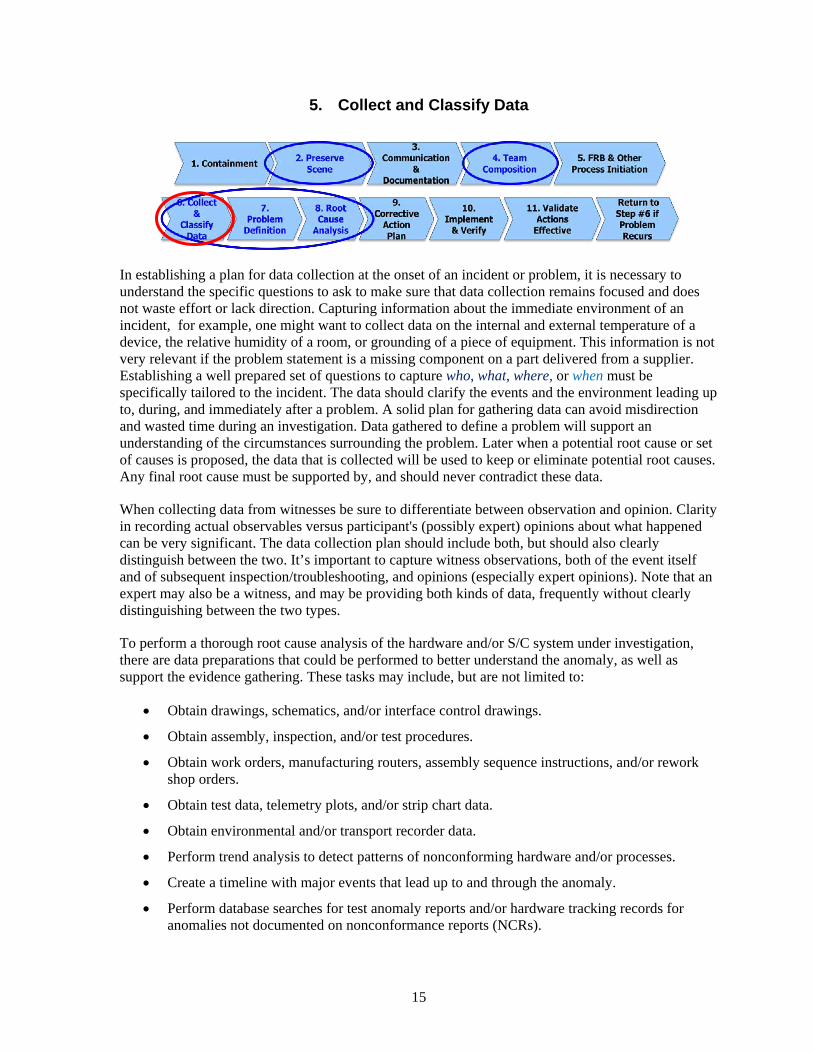
5. Collect and Classify Data

In establishing a plan for data collection at the onset of an incident or problem, it is necessary to understand the specific questions to ask to make sure that data collection remains focused and does not waste effort or lack direction. Capturing information about the immediate environment of an incident, for example, one might want to collect data on the internal and external temperature of a device, the relative humidity of a room, or grounding of a piece of equipment. This information is not very relevant if the problem statement is a missing component on a part delivered from a supplier. Establishing a well prepared set of questions to capture who, what, where, or when must be specifically tailored to the incident. The data should clarify the events and the environment leading up to, during, and immediately after a problem. A solid plan for gathering data can avoid misdirection and wasted time during an investigation. Data gathered to define a problem will support an understanding of the circumstances surrounding the problem. Later when a potential root cause or set of causes is proposed, the data that is collected will be used to keep or eliminate potential root causes. Any final root cause must be supported by, and should never contradict these data.

When collecting data from witnesses be sure to differentiate between observation and opinion. Clarity in recording actual observables versus participant's (possibly expert) opinions about what happened can be very significant. The data collection plan should include both, but should also clearly distinguish between the two. It’s important to capture witness observations, both of the event itself and of subsequent inspection/troubleshooting, and opinions (especially expert opinions). Note that an expert may also be a witness, and may be providing both kinds of data, frequently without clearly distinguishing between the two types.

To perform a thorough root cause analysis of the hardware and/or S/C system under investigation, there are data preparations that could be performed to better understand the anomaly, as well as support the evidence gathering. These tasks may include, but are not limited to:

• Obtain drawings, schematics, and/or interface control drawings.

• Obtain assembly, inspection, and/or test procedures.

• Obtain work orders, manufacturing routers, assembly sequence instructions, and/or rework shop orders.

• Obtain test data, telemetry plots, and/or strip chart data.

• Obtain environmental and/or transport recorder data.

• Perform trend analysis to detect patterns of nonconforming hardware and/or processes.

• Create a timeline with major events that lead up to and through the anomaly.

• Perform database searches for test anomaly reports and/or hardware tracking records for anomalies not documented on nonconformance reports (NCRs).

16

• Review NCRs on the hardware and subassemblies for possible rework, resulting in collateral damage.

• Review engineering change orders on the hardware and subassemblies for possible changes, resulting in unexpected consequences or performance issues.

• Interview technicians and engineers involved in the design, manufacture, and/or test.

• Perform site surveys of the design, manufacture, and/or test areas.

• Review manufacturing and/or test support equipment for calibration, maintenance, and/or expiration conditions.

• Review hardware and subassembly photos.

• Calculate on‐orbit, ground operating hours, and/or number of ON/OFF for the hardware and/or S/C system under investigation.

• Establish a point of contact for vendor/supplier communication with subcontracts.

• Obtain the test history of the anomaly unit and siblings, including the sequence of tests and previous test data relevant to the anomaly case.

As root cause team understanding expands, additional iterative troubleshooting may be warranted. Results from these activities should be fed back to the RCA team to incorporate the latest information. Additionally, troubleshooting should not be a trial-and-error activity but rather a controlled/managed process which directly supports RCA.

For each specific complex failure investigation a plan should be prepared which selects and prioritizes the needed data with roles and responsibilities. The investigation should be guided by the need to capture ephemeral data before it is lost, and by the need to confirm or refute hypotheses being investigated.

Some useful data collection and classification tools are summarized in Table 6 and described in detail in Appendix B.

Table 6. Data Collection and Classification Tools

Tool When to Use Check Sum When collecting data on the frequency or patterns of events, problems, defects,

defect location, defect causes, etc. Control Charts When predicting the expected range of outcomes from a process. Histograms When analyzing what the output from a process looks like. Pareto Chart When there are many problems or causes and you want to focus on the most

significant Scatter Diagrams When trying to determine whether the two variables are related, such as when

trying to identify potential root causes of problems. Stratification When data come from several sources or conditions, such as shifts, days of the

week, suppliers, or population groups. Flowcharting To develop understanding of how a process is done.

17

5.1 KNOT Chart

The KNOT Chart, shown in Figure 2, is used to categorize specific data items of interest according to the soundness of the information. The letters of the KNOT acronym represent the following:

Know: Credible Data

Need To Know: Data that is required, but not yet fully available

Opinion: May be credible, but needs an action item to verify and close

Think We Know: May be credible, but needs an action item to verify and close

The KNOT Chart is an extremely valuable tool because it allows the RCI investigator to record all information gathered during data collection, interviews, brainstorming, environmental measurements, etc. The data is then classified, and actions assigned with the goal of moving the N, O and T items into the Know category. Until data is classified as a K, it should not be considered factual for the purpose of RCA. This is a living document that can be used throughout the entire lifecycle of an RCA and helps drive data based decision making. One of the limitations is that verifying all data can be time consuming. Therefore, it can be tempting to not take actions on NOTs.

The KNOT Chart is typically depicted as follows:

Figure 2. KNOT chart example.

The first column includes a “Data” element that should be used later during the RCA as a reference to the KNOT Chart elements to ensure that all data collected has been considered.

5.2 Event Timeline

Following identification of the failure or anomaly, a detailed time line(s) of the events leading up to the failure is required. The purpose of the time line is to define a logical path for the failure to have

Kno

w

Nee

dto

kno

w

Opi

nion

Thin

kw

e kn

ow

Specific Data Item ActionD1 80% Humidity and Temperature of 84

degrees F at 2:00 PM

D2 Belt Speed on the machine appeared to be slower than usual

Locate and interview other witnesses

XX

Operator said she was having a difficult time cleaning the contacts

D3 X Locate and interview other witnesses

Press Head speed was set at 4500 rpmD4 X Verify by review of Press Head logs

D6

Oily Substance on the floor?D5 X Interview Cleaning Crew

Kno

w

Nee

dto

kno

wN

eed

to k

now

Opi

nion

Thin

kw

e kn

owTh

ink

we

know

Specific Data Item ActionD1 80% Humidity and Temperature of 84

degrees F at 2:00 PMD1 80% Humidity and Temperature of 84

degrees F at 2:00 PM



Locate and interview other witnesses

XX







D6


D6



18

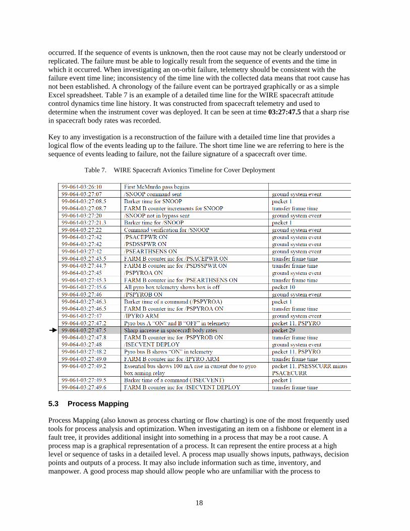
occurred. If the sequence of events is unknown, then the root cause may not be clearly understood or replicated. The failure must be able to logically result from the sequence of events and the time in which it occurred. When investigating an on-orbit failure, telemetry should be consistent with the failure event time line; inconsistency of the time line with the collected data means that root cause has not been established. A chronology of the failure event can be portrayed graphically or as a simple Excel spreadsheet. Table 7 is an example of a detailed time line for the WIRE spacecraft attitude control dynamics time line history. It was constructed from spacecraft telemetry and used to determine when the instrument cover was deployed. It can be seen at time 03:27:47.5 that a sharp rise in spacecraft body rates was recorded.

Key to any investigation is a reconstruction of the failure with a detailed time line that provides a logical flow of the events leading up to the failure. The short time line we are referring to here is the sequence of events leading to failure, not the failure signature of a spacecraft over time.

Table 7. WIRE Spacecraft Avionics Timeline for Cover Deployment

5.3 Process Mapping

Process Mapping (also known as process charting or flow charting) is one of the most frequently used tools for process analysis and optimization. When investigating an item on a fishbone or element in a fault tree, it provides additional insight into something in a process that may be a root cause. A process map is a graphical representation of a process. It can represent the entire process at a high level or sequence of tasks in a detailed level. A process map usually shows inputs, pathways, decision points and outputs of a process. It may also include information such as time, inventory, and manpower. A good process map should allow people who are unfamiliar with the process to

19

understand the workflow. It should be detailed and contain critical information such as inputs, outputs, and time in order to aid in further analysis.

The types of Process Maps are the following:

As-Is Process Map – The As-Is (also called Present State) process map is a representation of how the current process worked. It is important that this process map shows how the process works to deliver the product or service to the customer in reality, rather than how it should have been. This process map is very useful for identifying issues with the process being examined.

To-Be Process Map – The To-Be (also called Future State) process map is a representation of how the new process will work once improvements are implemented. This process map is useful for visualizing how the process will look after improvement and ensuring that the events flow in sequence.

Ideal Process Map – The ideal process map is a representation of how the process will work in an ideal situation with the constraints of time, cost, and technology. This process map is useful in creating a new process.

An example of a manufacturing process mapping flow diagram is shown in Figure 3 below:

Figure 3. Process mapping example.

20

6. Problem Definition

Before the root cause for an anomaly can be established, it is critical to develop a problem definition or statement which directly addresses the issue that needs to be resolved. When establishing the problem statement, the following elements should be considered:

• What happened? This statement needs to be concise, specific, and stated in facts, preferably based on objective data or other documentation. This statement should not include speculation on what caused the event (why?), nor what should be done next.

• Where did it happen? Where exactly was the anomaly observed? This may or may be the actual location where the event occurred. If the location of occurrence cannot be easily isolated (e.g., handling damage during shipment), then all possible locations between the last known ‘good’ condition and the observed anomaly should be investigated.

• Who observed the problem? Identification of the personnel involved can help characterize the circumstances surrounding the original observation, and understanding the subsequent access to those individuals may impact future options for root cause analysis.

• How often did it happen? Non-conformance research, yield data and/or interviews with personnel having experience with the affected hardware or process can aid in determining whether the event was a one-time occurrence or recurring problem, and likelihood of recurrence.

• Is the problem repeatable? If not, determination of root cause may be difficult or impossible, and inability to repeat the problem may lead to an unverified failure. If adequate information does not exist to establish repeatability or frequency of occurrence, consider replicating the event during the investigation process. Increased process monitoring (e.g., added instrumentation) while attempting to replicate the event may also help to isolate root cause. Other assets such as engineering units, brass boards, or residual inventory may be utilized in the RCA process so as not to impart further risk or damage to the impacted item. However, efforts to replicate the event should minimize the introduction of additional variables (e.g., different materials, processes, tools, personnel). Variability which may exist should be assessed before execution to determine the potential impact on the results, as well as how these differences may affect the ultimate relevancy to the original issue.

Other things to consider: • Title – A succinct statement of the problem using relevant terminology, which can be used

for future communication at all levels, including upper management and the customer • Who are the next level and higher customers? This information will aid in determining the

extent to which the issue may be communicated, the requirements for customer participation in the RCA process, and what approvals are required per the contract and associated mission assurance requirements.

• What is the significance of the event? Depending on the severity and potential impacts, the RCA process can be tailored to ensure the cost of achieving closure is commensurate with the potential impacts of recurrence.

21

Note the inability to adequately define and/or bound a problem can result in downstream inefficiencies, such as:

• Ineffective or non-value added investigative paths, which can lead to expenditure of resources which do not lead to the confirmation or exoneration of a suspected root cause or contributing factor.

• Incomplete results, when the problem statement is too narrow and closure does not provide enough information to implement corrective and/or preventive actions.

• Inability to close on root cause, when the problem statement is too broad, and closure becomes impractical or unachievable.

Figure 4 below is an example of a problem definition template.

Figure 4. Problem definition template.

22

7. Root Cause Analysis (RCA) Methods

In order to improve the efficiency or prevent recurrence of failures/anomalies of a product or process, root cause must be understood in order to adequately identify and implement appropriate corrective action. The purpose of any of the cause factor methods discussed here is to identify the true root cause that created the failure. It is not an attempt to find blame for the incident. This must be clearly understood by the investigating team and those involved in the process. Understanding that the investigation is not an attempt to fix blame is important for two reasons. First, the investigating team must understand that the real benefit of this structured RCA methodology is spacecraft design and process improvement. Second, those involved in the incident should not adopt a self-preservation attitude and assume that the investigation is intended to find and punish the person or persons responsible for the incident. Therefore, it is important for the investigators to allay this fear and replace it with the positive team effort required to resolve the problem. It is important for the investigator or investigating team to put aside its perceptions, base the analysis on pure fact, and not assume anything. Any assumptions that enter the analysis process through interviews and other data-gathering processes should be clearly stated. Assumptions that cannot be confirmed or proven must be discarded.

It is important to approach problems from different perspectives. Thus, the RCA processes include both “left-brain” logical techniques such as using a Fault/Failure Tree, Process Mapping, Fishbone Cause & Effect Diagram or Event Timeline as well as “right-brain” creative techniques such as Brainstorming. Regardless which RCA process is used, it is important to note that there are almost always more than one root cause and that proximate or direct cause are not root causes. The level of rigor needed to truly identify and confirm root causes is determined by the complexity, severity, and likelihood of recurrence of the problem. Included in the RCA techniques are methods that work well for simple problems (Brainstorming and 5-Why’s) as well as methods that work well for very complex problems (Advanced Cause & Effect Analysis and Process Mapping). As any RCA technique is applied, it is important to remember this about root cause: “The ultimate cause or causes that if eliminated would have prevented the occurrence of the failure.” In general they are the initiating event(s), action(s), or condition(s) in a chain of causes that lead to the anomaly or failure.

Root causes have no practical preceding related events, actions, or conditions.

Figure 5 provides some guidance when trying to decide what methods to use for simple versus complex problems.

7.1 RCA Rigor Based on Significance of Anomaly

In some cases it may be appropriate to reduce the level of RCA rigor if the issue is unlikely to recur, or if the impact of recurrence can be accommodated or is acceptable at a programmatic level (i.e., anticipated yield or ‘fallout’). Figure 6 may be used as guidance for determining the level of RCA rigor required: Based on the level of rigor from Figure 6, Figure 7 provides guidance for types of RCA methods which should be considered:

23

Figure 5. Recommended methods for simple versus complex problems.

Figure 6. RCA rigor matrix.

24

Figure 7. Example of RCA methods by RCA impact level matrix.

The following sections address commonly used RCA methods. Table 8 provides a summary of each method with pros and cons. A condition not discussed in each method but applicable to all is feedback. When the investigation team implements a method, it comes up with questions, then tasks troubleshooters to get more data or take a few more measurements. Then one updates the method until the next iteration. In addition as part of trouble shooting some analysts like the idea of isolating a fault geographically. For example; ‘A thruster doesn’t fire’, is the anomaly.

Step 1. Is the problem in the UUT or the test set? Answer, a logic analyzer shows the command was sent to fire the thruster, so the problem is in the UUT.

Step 2. Is the problem in the command decoder stage or the analog circuit that drives the thruster? Answer, troubleshooting shows the thruster fire command is decoded, so the problem is in the analog circuit. This process is continued until a particular bad part is found.

25

Table 8. RCA Methods Pros and Cons

RCA Method Pro Con Brainstorming (Sec 8.2)

Good technique for identifying potential causes and contributing factors.

Is a data gathering technique not a classification and prioritization process.

Cause and Effect Diagram (Fishbone) (sec 8.3)

Consideration of many different items Ability to plan, execute, and record results for multiple investigative paths in parallel. Simple graphical representation of a potentially large and complex RCA. Most commonly method used in industry.

Inability to easily identify and communicate the potential inter-relationship between multiple items. Best suited for simple problems with independent causes.

Fault Tree Analysis (FTA) (sec 8.4.4)

Help to understand logic leading to top event. Many software tools available NASA has an FTA Guide.

Requires knowledge of process. Fault Trees are typically used as a trial and error method in conjunction with a parts list.

Advanced Cause and Effect (ACEA) (sec 8.4.3)

Good tool for complex problems with dependent causes. Diligent scrutiny of cause and effect relationships of key factors and their inter-relationships.

Requires thorough understanding of cause and effect relationships and interactions. Higher commitment of resources and time in comparison to more basic tools.

Cause Mapping (sec 8.4.2)

Can be large or small, depending on the complexity of the issue. Introduces other factors which were required to cause the effect to create a more complete representation of the issue. Allows for clear association between causes and corrective actions, with a higher likelihood of implementation.

Difficult to learn and use.

Why-Why Charts (sec 8.4.1)

A good tool for simple problems with dependent causes. Also well suited for containment.

Typically based on attribute-based thinking, rather than a process perspective. Not as robust as some of the more advanced tools.

Process Classification Cause and Effect (CE) Diagram (sec 8.5.1)

They are easy to construct and allow the team to remain engaged in the brainstorming activity as the focus moves from one process step to the next. They invite the team members to consider several processes that may go beyond their immediate area of expertise. Invite the team to consider conditions and events between the process steps that could potentially be a primary cause of the problem. They often get many more potential root cause ideas and more specific ideas than might otherwise be captured in a brief brainstorming session.

Similar potential causes may repeatedly appear at the different processes steps.

26

RCA Method Pro Con Process Analysis (sec 8.5.2)

Excellent flowcharting method for complex problems with independent causes. Determines steps where defects can occur and defines factors or levels that would cause the defect.

Team-based methodology requiring knowledge of flowcharting.

RCA Stacking (combining Multiple RCA methods) (sec 8.6)

Allows simple tools to be used with a more complex method to find root causes quicker. 5-Why’s is simple and quicker to use and often used in conjunction with other methods.

Must go back and forth from one method to another – can cause confusion

7.2 Brainstorming Potential Causes/Contributing Factors

Following completion of the relevant portions of data collection/analysis activities, a key first step in the RCA process is to accumulate all of the potential causes and contributing factors. This step is often referred to as ‘brainstorming’, and the goal is to not only identify the most obvious root cause, but also to identify any possible underlying issues. The top level bones in an Ishikawa diagram can be used to provide reminders of categories that should be considered when identifying root cause hypotheses, and thus can serve as “ticklers” for a brainstorming session. One common RCA mistake is to identify and fix a problem at a too high a level, increasing the probability of recurrence.

Example: Multiple solder joint rejections are attributed to operator error, and the operator is reassigned based on the conclusion they did not have adequate skills to perform the task. A few weeks later, a similar solder operation performed by a different individual is rejected for the same reason. As it turns out, the company did not provide adequate training to the relevant process or specification. Had the true root cause been identified and addressed by subsequent training for all operators, the probability of recurrence would have been reduced.

It is preferable to not analyze or classify inputs at this time, as the logical arrangement of ideas can detract from the process. Brainstorming sessions are typically most productive when many ideas are brought forward without significant discussion, since classification and prioritization can take place once the methods and/or tools are selected.

All participants should be encouraged to identify any possible causes or contributors, and careful consideration of all ideas from team members typically encourages future participation. Also, no idea should be readily discarded, since by doing so the evidence against may not be adequately captured and available for subsequent RCA, team discussions, and/or customer presentations.

7.3 Fishbone Style

Figure 8 is commonly known as an ‘Ishikawa Diagram’ or ‘Fishbone Diagram’, this Cause and Effect Diagram is a method used to graphically arrange potential root causes into logical groups. The outcome is shown at the end of a horizontal line (the ‘head’ of the ‘fish’), and branches leading from this line identify the highest level category. Typically used categories (sometimes referred to as the ‘6Ms’) and examples are:

• Mother Nature (environment, surroundings)

• Material (physical items, requirements, standards)

• Man (people, skills, management)

27

• Measurement (metrics, data)

• Methods (process, procedures, systems)

• Machine (equipment, technology)

Note: These categories are suggestions only, and can be tailored to include other headings.

Potential root causes are then added to the relevant category, with the potential for one item being applicable to multiple categories. However, if during assignment of root causes this occurs repeatedly, it may be worth re-evaluating and identifying new categories.

Related causes are then added as progressively smaller branches, resulting in what appears to be a skeleton of a fish:

Figure 8. Ishikawa diagram (fishbone) example.

Diagram notes: 1) Potential root causes should be at the lowest level of a given branch. Higher levels should be used for grouping only. 2) Numbering items allows for cross-reference to an evidence table, which captures additional details and ultimately the rationale for disposition of a given item. 3) Color coding items by disposition aids in visualization, increasing efficiency during working meetings, and when communicating final outcomes.

Once all of the potential root causes are categorized and sub-branches identified graphically, supporting data can be associated with each item as the investigation proceeds. Arrangement of the potential root causes in this manner also helps to ensure that specific tasks, actionees, and due dates

28

are directly related to a specific item under investigation. Suggested tasks which do not promote the disposition of a given item should either be: a) rejected for lack of relevancy, or b) associated with a potential root cause which was not a part of the original brainstorming activity and should be added to the diagram.

Information regarding a specific item should be tracked in a supporting evidence table, which typically contains headers such as item number, description, reason for inclusion, open actions/actionees/due dates, results, and ultimately the final disposition for each individual item.

Several software tools can be used to produce this diagram such as Visio professional, iGRAFX Flowcharter, Powerpoint, etc. The advantages of a Cause and Effect Diagram include:

• Consideration of many different items

• Ability to plan, execute, and record results for multiple investigative paths in parallel

• Simple graphical representation of a potentially large and complex RCA

• Most commonly used method in industry

One commonly identified limitation of this method is the inability to easily identify and communicate the potential inter-relationship between multiple items.

7.4 Tree Techniques

7.4.1 5-Why’s

The 5-Why’s is a problem solving method which allows you to get to the root cause of a problem fairly quickly by repeatedly asking the question Why. Although five is a good rule of thumb, fewer or more may be needed. However, there becomes a point where the problem is no longer reasonably actionable.

5-Why’s analysis is a team-based process similar to brainstorming, designed to progressively probe the lower-tier causes of each potential cause. Using the tool is relatively simple:

• You first identify the problem statement

• Then ask Why the problem occurred (include multiple potential reasons if possible)

• Continue asking “Why” for each potential reason until the answers are identified as actionable root causes (stop when the answers become “unactionable” (like gravity, cold in Alaska, etc.)

• Systematically rule out items based upon objective evidence (such as test results, etc.) until actionable root causes are isolated

Note that the number “5” is purely notional; you continue asking “Why” as many times as is necessary until the answers become unactionable. An example of the 5-Why process follows in Figure 9:

29

Figure 9. Five Why process example.

To validate that there are true cause and effect relationships between items, read each branch backward and ask the question: If this cause is addressed, will the problem in the box before it be resolved? If not, then the causal item needs to be changed.

Although the 5-Why’s method may provide a quick and simple approach to problem solving, pursuing a single path may overlook other paths or interactions, potentially resulting in a sub-optimal root cause or an ineffective corrective action (see Cause Mapping).

7.4.2 Cause Mapping

Cause Mapping (also known as Apollo Root Cause Analysis Methodology) shown in Figure 10 is a graphical method which provides a visual explanation of why an event occurred. It is similar to the 5-Why’s method, but allows for multiple branches. Each causal box also includes the evidence that supports that specific cause. In addition, the Apollo RCA process also includes both “AND” and “OR” causal relationships. Cause Mapping connects individual cause-and-effect relationships to reveal the system of causes within an issue.

The advantages of a Cause Map include:

• Can be large or small, depending on the complexity of the issue

• Introduces other factors which were required to cause the effect to create a more complete representation of the issue

• Allows for clear association between causes and corrective actions, with a higher likelihood of implementation

30

Figure 10. Cause mapping methodology example.

7.4.3 Advanced Cause and Effect Analysis (ACEA)

The ACEA process shown in Figures 11 and 12 use cause and effect logic diagrams to define and document the logical relationships between the “Effect” (problem, anomaly, or unexpected event) and the various “Causes” (conditions, root causes, etc.) which contribute to it. The cause & effect relationships are more complex with this process since it utilizes both “OR” and “AND” relationships, and it also allows for the use of “SHIELDING” as opposed to elimination of root causes.

The steps in the ACEA process are as follows:

• Identify a chain of associated causes and effects

• Establish logical relationships (“or” or “and”)

• Identify potential solutions to eliminate or mitigate (“shield”) the causes

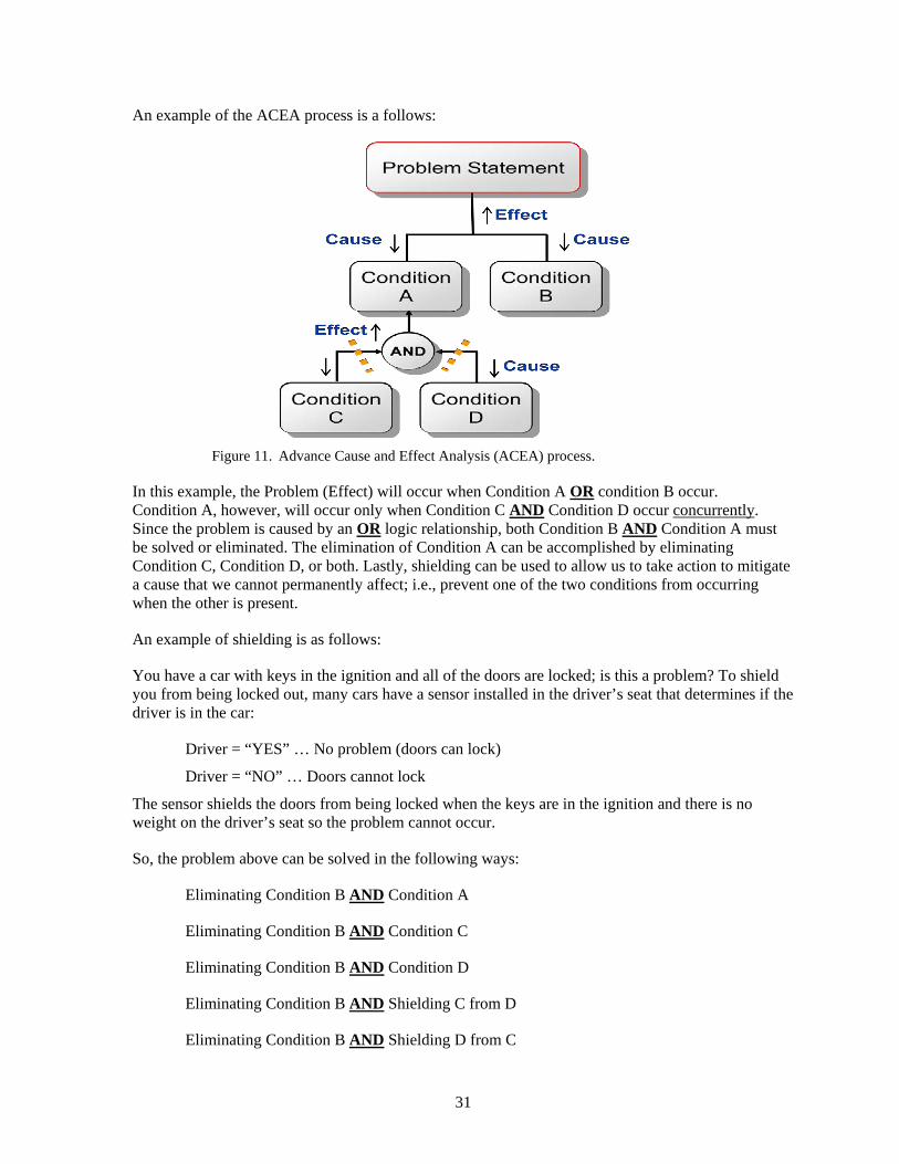
31

An example of the ACEA process is a follows:

Figure 11. Advance Cause and Effect Analysis (ACEA) process.

In this example, the Problem (Effect) will occur when Condition A OR condition B occur. Condition A, however, will occur only when Condition C AND Condition D occur concurrently. Since the problem is caused by an OR logic relationship, both Condition B AND Condition A must be solved or eliminated. The elimination of Condition A can be accomplished by eliminating Condition C, Condition D, or both. Lastly, shielding can be used to allow us to take action to mitigate a cause that we cannot permanently affect; i.e., prevent one of the two conditions from occurring when the other is present.

An example of shielding is as follows:

You have a car with keys in the ignition and all of the doors are locked; is this a problem? To shield you from being locked out, many cars have a sensor installed in the driver’s seat that determines if the driver is in the car:

Driver = “YES” … No problem (doors can lock)

Driver = “NO” … Doors cannot lock

The sensor shields the doors from being locked when the keys are in the ignition and there is no weight on the driver’s seat so the problem cannot occur.

So, the problem above can be solved in the following ways:

Eliminating Condition B AND Condition A

Eliminating Condition B AND Condition C

Eliminating Condition B AND Condition D

Eliminating Condition B AND Shielding C from D

Eliminating Condition B AND Shielding D from C

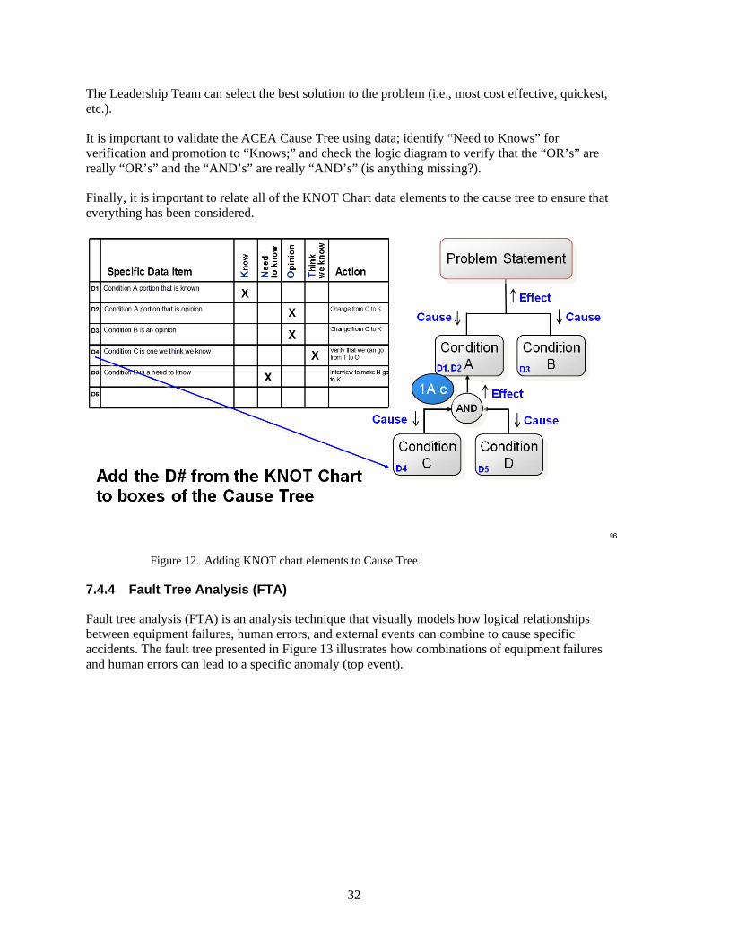
32

The Leadership Team can select the best solution to the problem (i.e., most cost effective, quickest, etc.).

It is important to validate the ACEA Cause Tree using data; identify “Need to Knows” for verification and promotion to “Knows;” and check the logic diagram to verify that the “OR’s” are really “OR’s” and the “AND’s” are really “AND’s” (is anything missing?).

Finally, it is important to relate all of the KNOT Chart data elements to the cause tree to ensure that everything has been considered.

Figure 12. Adding KNOT chart elements to Cause Tree.

7.4.4 Fault Tree Analysis (FTA)

Fault tree analysis (FTA) is an analysis technique that visually models how logical relationships between equipment failures, human errors, and external events can combine to cause specific accidents. The fault tree presented in Figure 13 illustrates how combinations of equipment failures and human errors can lead to a specific anomaly (top event).

33

Figure 13. Fault Tree Analysis (FTA) elements.

Below is a summary of the items most commonly used to construct a fault tree.

Top event and intermediate events

The rectangle is used to represent the TOP event and any intermediate fault events in a fault tree. The TOP event is the anomaly that is being analyzed. Intermediate events are system states or occurrences that somehow contribute to the anomaly.

Basic events

The circle is used to represent basic events in a fault tree. It is the lowest level of resolution in the fault tree.

Undeveloped events

The diamond is used to represent human errors and events that are not further developed in the fault tree.

AND gates

The event in the rectangle is the output event of the AND gate below the rectangle. The output event associated with this gate exists only if all of the input events exist simultaneously.

OR gates

The event in the rectangle is the output event of the OR gate below the rectangle. The output event associated with this gate exists if at least one of the input events exists.

34

Example of a RCA using fault tree analysis

Figure 14 is a partial example of fault tree analysis used during an accident investigation. Note that in this case, branches of the fault tree are not developed further if data gathered in the investigation indicate that the branch did not occur. These precluded branches are marked with “X’s” in the fault tree, and data are provided to defend the decisions. Each level of the fault tree is asking “why” questions at deeper and deeper levels until the causal factors of the accident are uncovered.

Figure 14. Fault Tree example.

7.5 Process Flow Style

7.5.1 Process Classification

A Process Classification CE diagram, as shown in Figure 15 is most useful when a known sequence of events or process steps precede the problem or unwanted effect. A Process Classification diagram is easy to construct. The problem statement (or the unwanted effect) is placed to the right end of the backbone of the diagram as in other CE diagrams. Along the backbone, however, are located blocks that represent the sequential events or process steps leading up to the problem. This can be considered

35

a linear time-based representation of the preceding events. From these blocks the team is asked to identify the potential causes, as they would on a typical CE diagram. The arrows between the process steps that form the backbone also have significance because they may represent opportunities for cause discovery that occur between the identified steps. The arrows may represent material handling events, documentation process delays, or even environmental changes from one location to another.

Figure 15. Example of process classification Cause and Effect (CE) diagram.

A well constructed Process Classification CE diagram has several distinct advantages.

They are easy to construct and allow the team to remain engaged in the brainstorming activity as the focus moves from one process step to the next.

They invite the team members to consider several processes that may go beyond their immediate area of expertise.

Invite the team to consider conditions and events between the process steps that could potentially be a primary cause of the problem.

They often get many more potential root cause ideas and more specific ideas than might otherwise be captured in a brief brainstorming session.

Disadvantages include

Similar potential causes may repeatedly appear at the different processes steps.

7.5.2 Process Analysis

The process analysis method is an 8 step process as follows:

Step 1: Flowchart the process

Step 2: Identify where the defects can occur

Step 3: Identify the factors where the defects can occur

Step 4: Identify the level of the factors which could cause the defect to occur

Step 5: Team identifies cause(s) to address

36

Step 6: Validate cause(s) via facts and data

Step 7: Update with findings and new potential cause(s)

Step 8: Repeat Steps 5-8 until causes are identified

Figure 16 is an example of the process analysis method.

Figure 16. Process analysis method example.

7.6 RCA Stacking

RCA Stacking, as shown in Figure 17, is the technique of using multiple root cause analysis tools to identify the underlying actionable causes of a nonconformity or other undesirable situation.

The steps in applying RCA Stacking are as follows:

Complete a basic investigation.

Including Problem Definition, Data Collection, and the generation of an RCA technique such as Fishbone Cause and Effect Diagram.

Determine if additional analysis is required.

Do the potential root causes listed on the Fishbone need more analysis in order to drill down to the true root causes?

Complete additional analysis.

Utilize another RCA technique such as a 5-Why Fault Tree to determine the true root causes of each item listed on the Fishbone.

Develop comprehensive output.

Include the results of the 5-Why on the Fishbone Diagram and C/A Plan.

37

Figure 17. RCA stacking example.

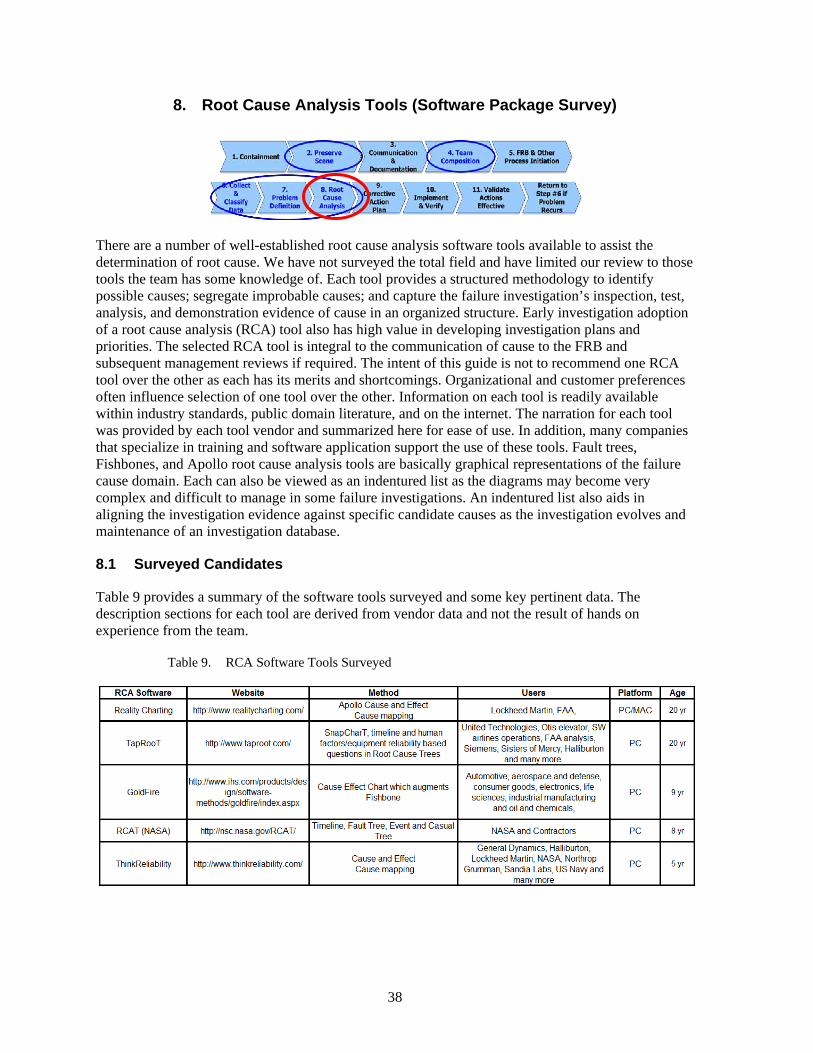
38

8. Root Cause Analysis Tools (Software Package Survey)

There are a number of well-established root cause analysis software tools available to assist the determination of root cause. We have not surveyed the total field and have limited our review to those tools the team has some knowledge of. Each tool provides a structured methodology to identify possible causes; segregate improbable causes; and capture the failure investigation’s inspection, test, analysis, and demonstration evidence of cause in an organized structure. Early investigation adoption of a root cause analysis (RCA) tool also has high value in developing investigation plans and priorities. The selected RCA tool is integral to the communication of cause to the FRB and subsequent management reviews if required. The intent of this guide is not to recommend one RCA tool over the other as each has its merits and shortcomings. Organizational and customer preferences often influence selection of one tool over the other. Information on each tool is readily available within industry standards, public domain literature, and on the internet. The narration for each tool was provided by each tool vendor and summarized here for ease of use. In addition, many companies that specialize in training and software application support the use of these tools. Fault trees, Fishbones, and Apollo root cause analysis tools are basically graphical representations of the failure cause domain. Each can also be viewed as an indentured list as the diagrams may become very complex and difficult to manage in some failure investigations. An indentured list also aids in aligning the investigation evidence against specific candidate causes as the investigation evolves and maintenance of an investigation database.

8.1 Surveyed Candidates

Table 9 provides a summary of the software tools surveyed and some key pertinent data. The description sections for each tool are derived from vendor data and not the result of hands on experience from the team.

Table 9. RCA Software Tools Surveyed

39

8.2 Reality Charting (Apollo)

The Apollo Root Cause Analysis (ARCA) process is described in the book Apollo Root Cause Analysis by Dean Gano. Apollo Root Cause Analysis was born out of the Three Mile Island Nuclear Power Plant incident of 1979 when Dean L. Gano was working in the nuclear power industry. It is an iterative process that looks at the entire system of causes and effects. ARCA is recommended for event/incident-based items of complex and higher significance.

Reality Charting is collaborative software used to graphically illustrate, with evidence, all of the causes, their inter-relationships, and effective solutions. The four steps of ARCA are:

• Determine Focus Areas and Define Problems

• Develop Cause and Effect Diagram with Evidence

- For each primary effect ask “why?” to the ‘point of ignorance’ or use ‘stop’

- Look for causes in ‘actions’ and ‘conditions’

- Connect causes with ‘caused by’

- Support causes with evidence or use a “?”

• Generate Potential Solutions

- Challenge the causes and offer solutions from ‘right’ to ‘left’

- Identify the ‘best’ solutions – they must:

Prevent recurrence

Be within your control

Meet your goals and objectives

• Implement and Mistake Proof

The Cause and Effect Continuum is illustrated in Figure 18 below:

Figure 18. Reality charting cause and effect continuum.

http://www.amazon.com/s/ref=nb_ss_gw?url=search-alias=aps&field-keywords=apollo+root+cause+analysis

http://www.amazon.com/s/ref=nb_ss_gw?url=search-alias=aps&field-keywords=apollo+root+cause+analysis

40

In investigating a root cause, the entire system of causes and effects is addressed. This method focuses on the condition causes versus the action causes to find more effective solutions, and prevent recurrence of undesired effects. Using the Reality Charting software, the output results in a typical diagram of a cause and effect continuum as shown in Figure 19.

Figure 19. Reality charting cause and effect chart example.

The cause investigations are stopped when the desired condition is achieved, or there is no control, or there is a new primary effect and persuing other causes would be more effective. Use of ARCA requires training by a facilitator, and it is not easily intuitive. The tool is most readily used when a complex failure investigation has multiple causes and effects.

8.3 TapRooT

TapRooT takes a completely different approach to how a root cause analysis process is used in an investigation. In the TapRooT 7-Step Process shown in Figure 20, the SnapCharT (Figure 21) is used throughout the investigation.

41

Figure 20. TapRooT 7-step process.

Planning

The first tool from the TapRooT toolbox that helps an investigator collect info is the SnapCharT. The investigator starts using this tool to organize the investigation and decide what evidence needs to be gathered and assigns a priority to securing evidence that might be lost.

Determine Sequence of Events and Casual Factors

The main tool they use for collecting evidence is the SnapCharT. Also used is Change Analysis, and Equifactor. This combination of advanced tools produces better information to analyze. The SnapCharT is a visual depiction of the evidence. It focuses the investigator on “What happened?” Any assumptions (not verified facts) are easily identified by their dashed boxes. The investigator then continues to look for more evidence to verify the assumptions or show a different, but also possible, sequence of events and conditions.

The SnapCharT different “seasons” determines the level of detail shown on the SnapCharT.

http://www.taproot.com/wordpress/wp-content/uploads/2011/01/201101071326.jpg

42

The Autumn SnapCharT includes all the Causal Factors and evidence needed to find the incident’s root causes. Occasionally, an investigator will discover additional information when using the Root Cause Tree to find root causes. This info needs to be added to the SnapCharT to make it complete.

Figure 21 below is an example of a SnapCharT.

Figure 21. TapRooT snap chart example.

Analyze Casual Factors for Root Cause

TapRooT’s tool for root cause analysis is the Root Cause Tree. The Root Cause Tree takes the knowledge of hundreds of experts and makes it available to every investigator. This knowledge doesn’t have to be in the investigator’s head; it is built into the Root Cause Tree and the Root Cause Tree Dictionary. Applying these systematic methods helps TapRooT users keep from jumping to conclusions.

The organization of causation in the Root Cause Tree not only came from many reliable, advanced sources but also was reviewed, critiqued, and tested. Beyond that, there are over 20 years of feedback from the international base of TapRooT Users and members of the TapRooT Advisory Board. This makes the TapRooT System a unique, advanced process for finding the real root causes of problems.

The TapRooT 5-Day Advanced Root Cause Analysis Team Leader Course includes cognitive interviewing combined with the TapRooT SnapCharT technique to improve interviews. This shifts the interviews from a questioning to a listening process. The cognitive interviewing process encourages interviewees to share all the info they know by encouraging them to remember. Also, the interviewee is told to provide details no matter how small or unimportant.

http://www.taproot.com/courses.php?d=2

43

Scale an Investigation

The TapRooT System is flexible to accommodate any size risk. Use some techniques for every investigation. Others are just applied in major investigations.

For simple incidents, a single investigator draws a simple SnapCharT of the sequence of events and identifies one to three easy-to-spot Causal Factors. They can do this working with those involved in a couple of interviews, just one or two hours total.

Drawing a SnapCharT is required because you have to understand what happened before you can determine why it happened.

Next, the investigator or team takes those Causal Factors through the Root Cause Tree. Perhaps an hour of work. Then another hour to develop some simple, SMARTER corrective actions based on the Corrective Action Helper Guide and to document it with some short written sections in the TapRooT Software. You are ready for approval, it takes about one half day’s work.

Investigating a large incident requires a full-blown investigation team with an independent facilitator; SnapCharT, Change Analysis, Equifactor, Safeguard Analysis, and the Root Cause Tree. Look for generic causes of each root cause. Then remove the hazard or target or change the human engineering of the system. If the appropriate investigation is a response in between, just do what you need based on the size of the problem. And if you discover that a problem is bigger than you thought, let management know and change the scope of the investigation.

8.4 GoldFire

Goldfire provides engineers and other technical and business professionals advanced research and knowledge-discovery tools. Goldfire provides access to internal scientific, technical, and business-development knowledge as well as a broad range of rich external content. It is a very large powerful tool with many uses. We will focus on the GoldFire Rapid Root Cause Analysis tool.

In the rush to resolution, engineers often solve only a symptomatic cause-resulting in rework or fault re-occurrence. Poor root cause analysis can increase companies’ total cost of ownership by as much as seven to ten percent. Given the impact of the lost revenues and opportunities, the expense of diverting key personnel resources, and the extended corporate liability, organizations are highly motivated to find a faster and better way to solve problems. Invention Machine’s Goldfire Innovator™ meets this need with a unique software solution that addresses the primary shortfalls of traditional approaches. By combining an automated problem analysis workbench with a patented semantic knowledge engine, Goldfire Innovator brings a structured and repeatable process that optimally leverages corporate expertise and external worldwide knowledge sources.

Simply solving or eliminating a problem is not always enough. Particularly when there is direct customer involvement, there is often a need to identify a root cause before initiating corrective action to verify the effectiveness of the solution, and to ensure there will be no unintended consequences. The standard approach to RCCA is to develop a fishbone diagram that separates potential causes into specific categories:

1. Equipment

2. Process

3. People

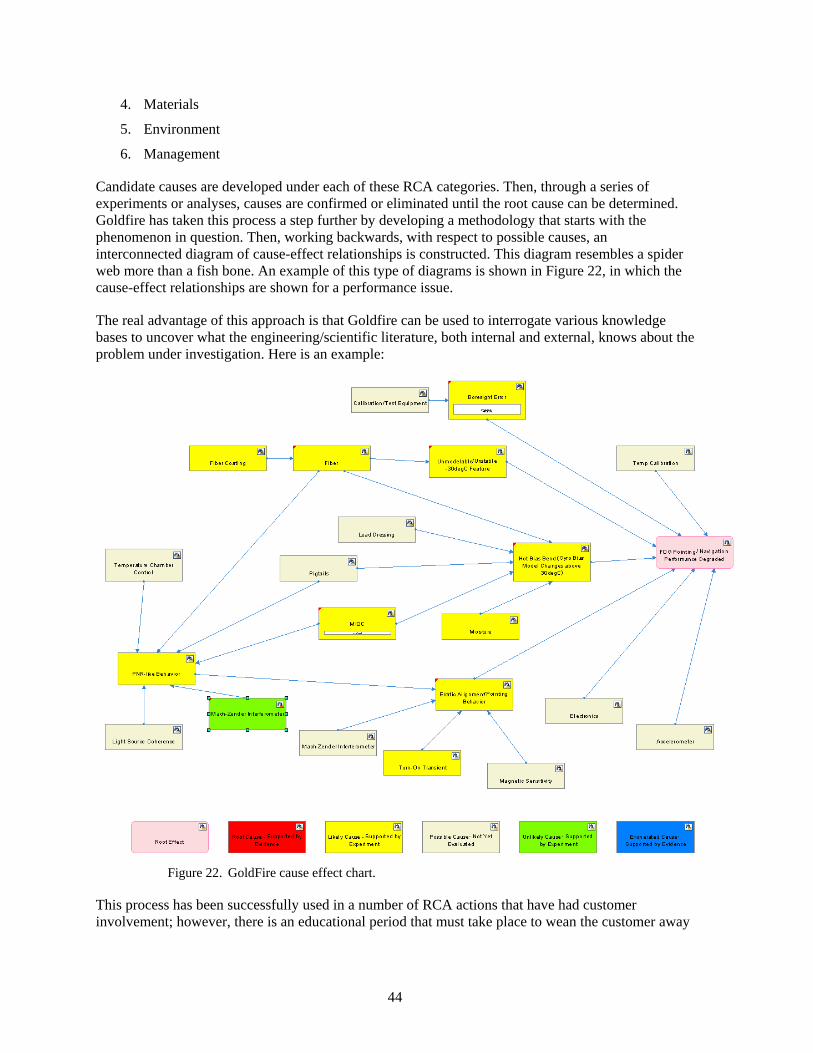
44

4. Materials

5. Environment

6. Management

Candidate causes are developed under each of these RCA categories. Then, through a series of experiments or analyses, causes are confirmed or eliminated until the root cause can be determined. Goldfire has taken this process a step further by developing a methodology that starts with the phenomenon in question. Then, working backwards, with respect to possible causes, an interconnected diagram of cause-effect relationships is constructed. This diagram resembles a spider web more than a fish bone. An example of this type of diagrams is shown in Figure 22, in which the cause-effect relationships are shown for a performance issue.

The real advantage of this approach is that Goldfire can be used to interrogate various knowledge bases to uncover what the engineering/scientific literature, both internal and external, knows about the problem under investigation. Here is an example:

Figure 22. GoldFire cause effect chart.

This process has been successfully used in a number of RCA actions that have had customer involvement; however, there is an educational period that must take place to wean the customer away

45

from the fishbone to this new approach, or at least to get customer concurrence that this approach may be pursued in parallel, since many customers are so accustomed to the fishbone process.

8.5 RCAT (NASA Tool)

Summary:

The Root Cause Analysis Tool (RCAT) was developed by NASA to address the specific needs of the space industry that were not presently available on the commercial off the shelf RCCA tools. The paper based tool with accompanying software is available free to all government agencies and contractors with NASA contracts.

Tool Overview:

RCAT is designed to facilitate the root cause and corrective action process in the space industry. Ideally, the RCAT software provides a framework to generate accurate and repeatable root cause investigations while helping to document that root cause and to identify corrective actions. The tool can also be used for trending analysis and data generation that can be used for further analysis or assessment.

While there are other RCCA tools on the market, NASA determined that those products were limited in their support of the comprehensive root cause analysis required in our industry. The NASA RCAT paper/software tool was developed to address this need and to provide it to government agencies and NASA contractors. Figure 23 below is the RCAT Introduction page.

Figure 23. RCAT introduction page.

46

Tool Functionality:

In contrast to the commercial tools, the NASA RCAT was designed to account for all types of activities and thus all types of potential causes of accidents in our industry (i.e., hardware, software, humans, the environment, weather, natural phenomenon, or external events), and allow them to be incorporated into the timeline, fault tree, and event and causal factor tree (5 Why). All of which make up the core of the tool. Specifically, the RCAT provides a step-by-step guide, logic diagramming capability, while using standard terminology, standard definitions, and standard symbols.

The RCAT software provides the user with a quick and easy method to perform the following:

1. Document case file properties

2. Identify and document the undesired outcome

3. Create and edit a detailed timeline

4. Create and edit a short timeline

5. Create and edit a fault tree

6. Create and edit an event and causal factor tree

7. Generate a report

8. Trend case file properties, causes, contributing factors, and other information

Pros and Cons:

• Pros Useful for complex RCA investigations with a lot of supporting information

Uses any combination of 3 root cause investigation methods

Timeline Fault Tree E&CFT (5-Why)

If items are fully implemented, creates comprehensive database of actors and actions

Recognized and accepted by NASA

Automated report generation

• Minuses

Restricted to NASA Contractors (but not restricted to NASA contracts)

Difficult to use and time consuming (impedes full implementation)

Full implementation needed to utilize database capabilities of actors and actions

NASA centric

Inherent parent structure between fault tree and E&CFT (5-Why)

47

Conclusion:

The tool can be very useful for data heavy root cause investigations, and the generated report is convenient, and welcomed by NASA. However, going to this system for straight forward investigations outside of your normal anomaly reporting system seems unlikely. Therefore, the database functionality of tracking actors and actions would be lost.

8.6 Think Reliability

Think Reliability

Think Reliability investigates errors, defects, failures, losses, outages and incidents in a wide variety of industries. Their Cause Mapping analysis method of root causes captures the complete investigation in an easy to understand format. Think Reliability provides investigation services and root cause analysis training to clients around the world.

The Cause Mapping Method of Root Cause Analysis

A Cause Map, as shown in Figure 24, provides a simple visual explanation of all the causes that were required to produce the incident. There are three basic steps to the Cause Mapping method:

Figure 24. Think reliability cause mapping steps.

1. Define the issue by its impact and risk to the overall goals

2. Analyze the causes in a visual map supported with evidence

3. Prevent or mitigate any negative impact and risk to the goals by selecting the most effective solutions

A Cause Map provides a visual explanation of why an incident occurred. It connects individual cause-and-effect relationships to reveal the system of causes within an issue. A Cause Map can be very basic and it can be extremely detailed depending on the issue. You can document the information with pen and paper, using dry-erase boards, on chart paper, or electronically in Microsoft Excel.

48

How to Read a Cause Map

As shown on Figure 25, start on the left. Read to the right saying “was caused by” in place of the arrows. Investigating a problem begins with the problem and then backs into the causes by asking Why questions. A Cause Map always begins with this deviation which is captured as the impact to the organizations overall goals.

Figure 25. Reading a cause map.

Figure 26 is an example of a cause map for –The Sinking of the Titanic.

Figure 26. Example – sinking of the Titanic cause map.

49

9. When Is RCA Depth Sufficient

Root Cause Analysis is the use of a set of methods and tools to create a confident understanding of the causes leading to particular event. Ideally, the depth of the root cause analysis is sufficient when those underlying cause are sufficiently understood to allow the prevention of recurrence. This includes, again in the ideal case, complete resolution of all of the possible causes (branches of the fishbone or fault tree) as either exonerated, or, for those causes that can or have contributed to the event, that the mechanisms of the failure are clearly understood, as are corrective actions which will conclusively prevent recurrence of the failure.

However, in practice this level of understanding is unlikely to be achieved, either because a specific set of root causes cannot be identified, or certain hypotheses (branches) cannot be conclusively exonerated or implicated in the failure in a resource constrained environment. While the constraining resource can in principle be technical, cost, or time (schedule), the constraint is usually not technical. Regardless of the specific constraint, at this point the depth of the root cause analysis needs to be assessed to determine if the existing analysis is sufficient, even if it is not complete.

To assess this, it is important to understand (and have common terminology to discuss) “cause” in two different ways: from the standpoint of the causal chain, and from the standpoint of the certainty of understanding.

The causal chain is the interrelationship between cause and effect leading to the observed event. In some cases, this may include all of the cause and effect relationships that could lead to the observed event, regardless of which sequence actually resulted in the particular event in question. The “causal chain” is so-called because there is a chain of cause and effect relationships reaching back from the observed event. Each effect, starting with the event in question, has a proximate (also called the direct or immediate) cause (or causes). This proximate cause is the event that occurred, including any condition(s) that existed immediately before the undesired outcome, directly resulted in its occurrence, and, if eliminated or modified, would have prevented the undesired outcome. Since this proximate cause is itself an undesirable event, it too has its own proximate cause, and so on. This chain can be extended essentially indefinitely. Branches may occur in the causal chain, for example when two different causes could lead to the same event; for a complete analysis each branch would have to be pursued to its full depth. We define a cause as a (or the) root cause — the “ultimate cause or causes that if eliminated would have prevented the occurrence of the failure” — when the analysis has reached sufficient depth (and breadth) to allow for the determination of effective actions that can be taken to prevent re-occurrence of the failure in the same design. Frequently, this means that there may be “root” causes at several levels, depending on what actions are considered feasible. So a practical concept of how deep the root cause analysis needs to go is deep enough so the team is satisfied that corrective action can be proposed that is both implementable and will reliably prevent re-occurrence.

Determination of a stopping point for RCI depends on different factors (practicality, cost, schedule, etc). Ideally, root cause analysis should be performed until no more actionable items exist. However, determining a stopping point should be the recommendation of the investigation team and a decision then should be made by the investigation sponsor.

50

In assessing the depth of root cause analysis, there are three key levels of depth, corresponding with the levels of action taken to correct the problem. The first two levels of action are remedial and corrective actions, which eliminate or correct the nonconformance and prevent recurrence of the failure within the sibling units of the same design. Since typically, only remedial and corrective actions are under the control of a program-funded investigation, completion at this level of RCI (and corrective action) should satisfy the contractual scope. However, specifics of each contract should be consulted.

At a deeper third level, preventive action can be put in place to prevent recurrence of similar problems across similar designs [see Ref 1. FRB TOR-2011(8591)-19]. Which level of action is desired is part of the defined scope of the analysis, and should be captured in the problem statement. In many cases, the initial analysis will be chartered to identify sufficient depth to enable corrective action, which is commonly program specific; further depth may then be handed off to an organizational/functional investigation. In some cases, the initial investigation team may be chartered to continue the investigation through the broader organization as preventive action. It is important for the team to have a clear problem statement and a means of escalating the decision of how deep the investigation should go, and who is paying for that deeper investigation.

In addition to the question of depth of the analysis, sufficiency of the analysis must also consider the breadth of the analysis. In other words, has the analysis considered the full range of causes appropriate to the undesired effect.

Here is a list of questions that may be asked within the team to determine if the depth has been sufficient:

1. Are there multiple potential contributing causes identified? The team should consider that while each contributor alone may not be sufficient, there are interactions of potential contributors that may be the root cause, whereas none of the issues alone would be sufficient. The interactions that could be significant should be vetted to the degree possible. For example, there may be considerable variation in manufacturing stresses and considerable variation in material strength. Failure occurs in only rare instances where the outlying high stress exceeds the outlying low strength.

2. Was the problem set up accurately by creating a list of Key Facts? The investigation team needs to take care that they did not assume something basic was a fact when it was actually a supposition. Was the team subject to “target fixation”? That is, did they assume they “knew” what the failure was from the beginning (perhaps based on a known process change) as opposed to performing an unbiased, impartial review? Care needs to be taken that the team did not fixate on collecting data to support a “known” theory and ignored key facts that didn’t fit their presupposition.

3. What is the potential impact to the particular spacecraft or fleet of spacecraft if further investigation is curtailed? If there is minor or no impact, then escalation to upper management and the affected customer may be appropriate to verify if the team needs to keep going. While Root Cause Analysis is not time based, it can be time bound. Will anything be impacted if the activities are curtailed, or is the concern “overcome by events”?

4. Is there any contradictory evidence to the root cause? If there is contradictory evidence remaining, the depth is probably not sufficient and further investigation is needed. The selected Root Cause(s) should explain every fact identified during the data collection, and must not contradict any of the facts.

51

5. Is there anything else that can be done? If there are no more data that can be obtained and reviewed (more likely for certain on-orbit investigations than for failures on the ground) then activities may be curtailed. Another similar case is where the root cause, while identified, is unchangeable or no longer relevant.

6. Have the open fishbone or fault tree branches been vetted thoroughly through representative testing? If not, then additional testing may be appropriate.

7. Has the team reached only proximate cause, or has the team gone deep enough into the underlying cause? For example, if root cause analysis identifies human error as the proximate root cause, the process should be continued until the underlying latent cause is identified, which allowed the human proximate cause to happen. This human error could, for example, be a lack of training, a lack of correct procedures, or a lack of management oversight.

8. Was the right expertise on the team? Impartial outside subject matter experts or failure investigation experts may be called in for a fresh opinion and impartial review.

9. Have corrective actions for each potential cause contributor been implemented to prevent recurrence? It may be acceptable to curtail activities if all corrective actions for all credible and likely causes have been implemented, even if one particular cause could not be identified.

10. Was a sufficiently rigorous RCA technique chosen?

So far, the discussion of causation has implicitly assumed that we have perfect understanding of the cause and effect relationships involved in the analysis. Frequently, this is not true. As a result, we may label a proposed (root) cause as a probable cause. Formally, a probable cause is a cause identified, with high probability, as the root cause of a failure but lacking in certain elements of absolute proof and supporting evidence. Probable causes may be lacking in additional engineering analysis, test, or data to support their reclassification as root cause and often require elements of speculative logic or judgment to explain the failure. The core of this formal definition is that we are not completely certain of all of the cause and effect relationships involved, theoretically or actually, in the proposed causal chain although we have a “high” confidence in our explanation.

If our understanding of the causal chain does not merit high confidence, we enter the realm of the unverified failure (UVF), and unknown direct or root causes. All of these terms (which have specific shades of meaning; see Section 3) express different, low, levels of uncertainty in understanding of the causal chain, and terminating the analysis under these conditions implies increased risk of re-occurrence — which is usually undesirable. Dealing with these situations is discussed in Section 12 below.

The ultimate proof of the root cause analysis is in the validation of the corrective actions taken as a result of the analysis. While a detailed discussion of this step of the RCCA process is beyond the scope of this guide, and even the absence of recurrence in a limited production run may not be complete proof of the validity of the corrective actions, the effective prevention of recurrence is both the goal of the RCCA process and the ultimate measure of the effectiveness of the root cause investigation.

9.1 Prioritization Techniques

9.1.1 Risk Cube

Using a two by two matrix as shown in Figure 27, the following 5 instructions follow:

1. Identify potential solutions using the results of the root cause analysis

52

2. Enter potential solution descriptions on the right of the template

3. Drag each solution to appropriate location on the solution selection square

4. Select solutions using guidance provided here

5. Develop CAP based upon the results of step 4

The team may wish to pursue those root causes and/or solutions in the high priority green area (i.e., high success/benefit w/low difficulty/cost); whereas, those in the red area (i.e., low success/benefit w/high difficulty/cost) would likely be the lowest priority. For the yellow areas (i.e., high/high and low/low), develop justification/ROI and implement only as a medium priority if the green solutions are ineffective.

Figure 27 . Root cause prioritization risk cube.

9.1.2 Solution Evaluation Template

The template shown in Figure 28 is a spreadsheet that can be used to help determine which solutions should be pursed based on quantitative data. The process is essentially the following three steps.

1. Populate solutions on the spreadsheet

2. Evaluate each solution using the relative score based upon the following criteria:

a. Probability of correcting problem

b. Whether solution is within team’s control

c. Whether solution could create new problem

d. Difficulty to implement

e. Cost to implement

3. Select solutions

53

Figure 28. Solution evaluation template.

54

10. RCA On-Orbit versus On-Ground

Anomalies associated with deployed systems can be substantially more difficult to investigate as compared to ground-based anomalies, often due to a lack of evidence and/or the ability to replicate the problem. In these situations, analysis of telemetry directly associated with the anomaly is often the most viable option. Pursuit and investigation of supplemental telemetry data from other subsystems – whether initially deemed to be relevant or not – may also provide ‘indicators’ which can assist in the RCA.

Example: Attitude control and determination data might shows that an in-orbit attitude control issue on a deployed satellite system could have led to a reduction in solar power, which in turn led to a loss of battery power and ultimately a transition to safe mode. Review of power telemetry alone may have prevented association to an orbital control issue.

Precursor telemetry should be analyzed when available, as it may provide indicators of the pending anomaly. Finally, other external factors should be considered, such as space weather or other unanticipated environments.

The RCA team may also have difficulty obtaining pre-launch build and test data, due to an inability to obtain internal historical records and/or supplier archives. Most contracts and subcontracts include data retention requirements; however, these may or may not exist, may not be effectively flowed to suppliers, or may expire before the anomaly is encountered. Therefore, data retention requirements should be established and understood early in the program lifecycle and reviewed periodically to ensure this information is available in the future if needed.

Exercising the affected item (i.e., repeating steps which led to the anomaly) and possibly varying parameters which led to the anomaly may aid in root cause determination. However, returning to a state where the anomaly occurred may result in further error propagation, or worst case a total loss of the asset. If the anomaly occurs after handoff of operation or ownership, there may also be resistance from the owner or operator to alter subsequent operations to support RCA, as this may create interruptions in service to the end customer. The risk of further impacts need to be understood and traded off against the potential benefit of establishing root cause.

Fault isolation trees can also aid in the diagnosis of an anomaly. Using the product structure of the affected item can aid in the evaluation of many possible contributors in parallel, and can also be used to eliminate various subsystems when adequate rationale has been established.

If the affected asset cannot be used for further RCA, other residual assets may be used to replicateroot cause, provided they are representative of the affected item. Such assets may include:

• Engineering or Qual Models

• Flight Spares

• Simulators or test benches

55

• Follow-on or other program assets (i.e., recurring builds still in-process)

• Supplier products or data

Again, the risks associated with exercising other assets need to be traded with the potential benefits to RCA.

In general, the ability to establish root cause for operational assets (especially those in-orbit) is often constrained by limited information associated with the original event, risk of failure propagation, risk of initiation of similar failures on redundant systems, inability to replicate the issue on similar hardware and/or operational considerations. Ultimately, the RCA is more likely to conclude with a ‘most probable root cause’ in these situations.

Although separate from understanding Root Cause, due to the constraints listed above, on-orbit anomalies also have the increased potential to result in an unverified failure (see below). Added telemetry functions should be considered for incorporation on designs which have shown susceptibility to degradation or failure, in order to provide additional data for future RCA in the event of recurrence.

56

11. RCA Unverified and Unknown Cause Failures

Practical considerations may sometimes render a particular failure not amenable to a root-cause determination. This can lead to an alternate process that deals with Unverified Failures or Unknown Cause Failures—the absence of the failure after implementing Remedial actions does not prove the effectiveness of the actions. Sometimes programmatic considerations (cost, schedule, safety of the system or component or personnel) may limit the scope of an investigation and make an accurate determination of direct causes impossible. In either case, the absence of definitive information about direct causes makes subsequent analyses of root causes highly speculative and requires significant effort to determine risk of proceeding without a determined root cause.

11.1 Unverified Failure (UVF)

An Unverified Failure (UVF) is a failure in hardware, software, or firmware in the UUT such that failure cannot be isolated to the UUT nor to the test equipment. Transient symptoms usually contribute to the inability of attributing a UVF to a direct cause. Typically a UVF does not repeat itself, preventing verification. UVFs do not include failures in the test equipment once they have been successfully isolated there. UVFs have the possibility of affecting flight units after launch. Like on-orbit anomalies, fault isolation and/or failure tree diagrams will be necessary and all potential RC’s must be addressed (i.e., eliminated, exonerated, shielded, etc.). When circumstances and supporting evidence prevent direct cause from being determined, three possibilities exist regarding knowledge as to the source of the failure.

1. It may be possible to determine the source of the failure is the support equipment.

2. It may be possible to determine the source of the failure is the flight system.

3. It may not be possible to determine if the source of the failure is the flight equipment or the support equipment.

The phrase “failure not verified” or “unverified failure” is sometimes used to describe this type of failure. After parsing the types of failures that resist direct cause investigations, two types remain that are threats to flight systems:

1. Failures that are known to originate in flight equipment (possibility 2 above)

2. Failures that may or may not originate in flight systems (possibility 3 above)

In the event of an UVF, a wide range of understanding and supporting evidence can exist regarding failures where the cause cannot be definitively determined. Examples include failures that appear to “self-heal” and are not repeatable, or when the majority of the evidence supports a “most probable” cause but confounding supporting evidence exists for other possible causes. Unless the failure is at a very low level of the system hierarchy and has very low consequences if it re-occurs, a Senior FRB is considered a highly recommended best practice. In addition unverified failures should be independently assessed to ensure that the risk baseline has not been unacceptably increased.

57

An example of an Unverified Failure is the following: a digital receiver processor box performed an uncommanded software reset during ambient electrical testing. Normal reset recovery did not occur because the flight software had been erased by the full power up sequence. After completion of 960 hours of powered on testing, the failure did not repeat. Circuit analysis and trouble-shooting indicated that the most probable cause was scintillation of a tantalum capacitor in the affected circuit. An independent subject matter expert on tantalum capacitors confirmed that scintillation was the most likely cause. Further environmental testing resulted in no recurrence of the failure.

In most cases, UVFs require a Worst Case Change Out (WCCO) performed on suspect hardware and software to minimize mission risk. If a WCCO is not performed then an independent UVF review team (depending upon the evaluated mission severity) should approve the mission risk. The composition of the UVF Review Team is dependent upon the mission severity. For those failures determined to have mission severity of loss or partial loss of redundancy, reduced mission data, increased complexity, or no mission impact, the UVF Review Team will be composed of independent and program/product area personnel. For those UVFs determined to have mission severity of mission loss, reduced mission life, or degraded mission the UVF Review Team should consist of senior level reviewers. Table 10 below illustrates a risk assessment process that can be performed for UVFs.

Table 10. UVF Risk Assessment Process Example

Mission severity (no WCCO) UVF Review Team Approves Mission loss Program Manager and Senior level review team Reduced mission life or degraded mission Loss of redundancy Program Manager, Mission Assurance, Quality Assurance,

Chief Engineer

Reduced mission data or partial loss of redundancy or increased operational complexity No mission impact Worst case change out approved disposition

Program Manager and Mission Assurance

Table 11 is a representative checklist or criteria to consider when a failure investigation ends without root cause being determined. Caution should be used when halting an investigation prior to determining root cause as it may become necessary to implement many other corrective actions to address all possible causes.

Table 11. UVF Verification Checklist

Number UVF Question 1 What was the nonconformance? Describe all significant events leading up to the occurrence.

Describe the trouble shooting conducted and the results. Note: A Fishbone Analysis or FMEA is recommended as an aid in presenting this data. Describe how each possible source of the nonconformance was dispositioned.

2 What was the test hardware/software configuration at the time of the nonconformance (i.e., if at system test, were all flight items installed)? Were some non-flight items installed? If at subsystem or unit level, were all flight components installed?) Describe the level of any software in use at the time of the nonconformance, if applicable (i.e., was flight code installed at the time of the nonconformance)?

3 What test was in process and were multiple tests being performed simultaneously? 4 Did the nonconformance repeat or were there any attempts to repeat the nonconformance? If so,

what was the result? Also, describe any troubleshooting performed while the nonconformance was present.

5 If the nonconformance cleared, what happened to cause the nonconformance to clear? What efforts were made to get the nonconformance to repeat? Were the hardware/software configurations identical to the original condition? If not, what were the differences, why were the differences necessary?

58

Number UVF Question 6 Was there any cumulative “nonconformance free” testing or re-testing that occurred after the

event(s)? 7 Does a failure analysis of the problem clearly lead to assigning the nonconformance to a specific

part or product? Was that part or product replaced? If so, when the part or product was fixed, was the problem cleared?

8 What would be required to perform a worst-case rework/repair? Was that performed? If not, describe the reason.

9 Did the nonconformance cause any overstress (consequential impact)? Is the overstress analysis documented? If not addressed, what was the rationale for not addressing the overstress issue?

10 Are there other relevant failures on other items or systems? If the failure is in a component/piece part, what is the failure history of that part? How many units have been built and what is their performance record?

11 If the nonconformance was traced to a part, what were the results of the failure analysis/DPA (e.g., did destructive physical analysis [DPA] confirm the failure)?

12 Were any troubleshooting steps considered and not performed due to cost or schedule concerns? Could these troubleshooting steps determine the cause of the nonconformance? Describe the reasonableness/risk in performing this troubleshooting now.

13 Are there operational workarounds possible to mitigate the effect of this nonconformance? Could they be implemented within the mission?

11.2 Unknown Direct/Root Cause Failure

An Unknown Direct Cause Failure is a repeatable/verifiable failure condition of unknown direct cause that cannot be isolated to the UUT nor to the test equipment.

An Unknown Root Cause Failure is a failure that is sufficiently repeatable (verifiable) to be isolated to the UUT or the Test Equipment, but whose root cause cannot be determined for any number of reasons.

The phrase “unknown direct cause” is sometimes used to describe failures isolated either to the UUT or the support equipment, whose direct cause cannot be found. Some failures do not provide sufficient evidence for the investigation team and FRB to determine if the cause originates in the flight system or the support systems. These failures typically involve transient symptoms. For these failures, the symptoms usually “evaporate” before it is possible to isolate the source of the failure to the flight or support systems.

An example of an Unknown Direct Root Cause Failure is the following: An electronic box fails during acceptance testing. Through investigation the failure is traced to a circuit board in the box and confirmed at card level. At this point the rest of the box is exonerated. Additional investigation traces the circuit board failure to a piece part, and the failure is again confirmed at the piece-part level. At this point the rest of the circuit board is exonerated. The piece part is taken to a Failure Analysis Laboratory, but root cause of the piece part failure cannot be determined. A new piece part in the circuit board results in acceptable test results. Appropriate actions to be taken at this stage would include additional investigation into the piece part’s history (e.g., lot date code (LDC), Destructive Physical Analysis results, usage of the LDC in other cards), a circuit overstress assessment based upon the part failure effect on other parts in the circuit (and whether an overstress caused the part to fail), and a margin assessment of the part in the circuit (similar to a Worst Case Analysis). The results of these efforts would be included in a completed UVF Engineering Analysis.

Since a failed piece part can be either a root cause or a symptom of another root cause, it is imperative that piece part failure analysis be thoroughly conducted. All potential failure modes are rigorously assessed for credibility. The observation of a failed piece part cannot be assumed to be the root cause of a failure. Care should be exercised to ensure that overstress, design features, failure of other piece

59

part(s), or other environmental factors are considered in determining the true root cause; in which case, the observed piece part failure is considered a consequence of the failure and not the root cause itself.

For Unknown Direct Cause and Unknown Root Cause failures, an Engineering Analysis and mission severity evaluation, as previously described, should be performed.

60

12. RCA Pitfalls

Some reasons the team observed for missing the true root cause include the following:

1. Incorrect team composition: the lead investigator doesn’t understand how to perform an independent investigation and doesn’t have the right expertise on the team. Many times specialty representatives, such as parts, materials, and processes people are not part of the team from the beginning.

2. Incorrect data classification: Investigation based on assumptions rather than objective evidence. Need to classify data accurately relative to observed facts.

3. Lack of objectivity/incorrect problem definition: The team begins the investigation with a likely root cause and looks for evidence to validate it, rather than collecting all of the pertinent data and coming to an objective root cause. The lead investigator may be biased toward a particular root cause and exerts their influence on the rest of the team members.

4. Cost and schedule constraints: A limited investigation takes place in the interest of minimizing impacts to cost and schedule. Typically the limited investigation involves arriving at most likely root cause by examining test data and not attempting to replicate the failed condition. The actual root cause may lead to a redesign which becomes too painful to correct.

5. Rush to judgment: The investigation is closed before all potential causes are investigated. Only when the failure reoccurs is the original root cause questioned. “Jumping” to a probable cause is a major pitfall in root cause analysis (RCA).

6. Lack of management commitment: the lead investigator and team members are not given management backing to pursue root cause; quick closure is emphasized in the interest of program execution.

7. Lack of insight: Sometimes the team just doesn’t get the inspiration that leads to resolution. This can be after extensive investigation, but at some point there is just nothing else to do.

8. Your knowledge (or lack of it) can get in the way of a good root cause analysis.

a. Experienced investigators often fall into the confirmation bias trap. They use their experience to guide the investigation. This leads them to find cause and effect relationships with which they are familiar. They search for familiar patterns and disregard counter evidence. The more experienced the investigator is the more likelythey are to fall into the trap.

b. Inexperienced investigators don’t know many cause and effect relationships. They can’t find what they don’t know. To combat the lack of knowledge, teams of investigators are assembled with the hope that someone on the team will see the right answer. Team effectiveness depends on team selection to counter the inherent weakness of the assumption behind cause and effect. Also, it assumes that the rest of the team will recognize the right answer when another team member suggests it. More likely, a “strong” member of the team will lead the team to arrive at the answers that the strong team member is experienced with.

61

13. References

The following list is provided to assist the community in establishing a common terminology for the practice of conducting Root Cause Analysis in support of space system failure review boards (FRBs) for failures on the ground and on-orbit.

1. TOR-2011(8591)-19 “Failure Review Board Guidance Document”

2. TOR-2013-00293 “Mission Assurance Practices for Satellite Operations”

3. NASA Safety Center (NSC) System Failure Case Studies http://nsc.nasa.gov/SFCS/

4. NASA Fault Tree Handbook http://www.hq.nasa.gov/office/codeq/doctree/fthb.pdf

5. NASA Procedural Requirements for Mishap and Close Call Reporting, Investigating, and Record Keeping http://nodis3.gsfc.nasa.gov/displayDir.cfm?Internal_ID=N_PR_8621_001B_&page_name=Chapter3

6. TOR-2009(8591)-13 “Space Vehicle FMECA Guide”

7. Root Cause Analysis Handbook, Third Edition, 2008, ABS Consulting www.ABSConsulting.com/RCA

8. Guide to Quality Control, Ishikaoru, K. 2nd Revised Ed., Asian Productivity Organization, JUSE Press, Tokyo, Japan, 1968

9. Apollo Root Cause Analysis- A New Way of Thinking, Gano, D.L. 2nd Ed., Apollonian Publications, Yakima, Washington, 2003

10. Reality Charting --- Seven Steps to Effective Problem-Solving and Strategies for Personal Success, Gano, D.L. 2nd Ed., Apollonian Publications, Richland, Washington, 2011

11. Effective Problem Solving Practitioners Guide, Automotive Industry Action Group, Southfield, Michigan, 2013

12. Practical Software Measurement: Measuring for Process Management and Improvement, Florac, W.A., Park, R.E., Carleton, A.D., Software Engineering Institute, Carnegie Mellon University, Pittsburgh, Pennsylvania, April 1997

http://nsc.nasa.gov/SFCS/

http://www.hq.nasa.gov/office/codeq/doctree/fthb.pdf

http://nodis3.gsfc.nasa.gov/displayDir.cfm?Internal_ID=N_PR_8621_001B_&page_name=Chapter3

http://nodis3.gsfc.nasa.gov/displayDir.cfm?Internal_ID=N_PR_8621_001B_&page_name=Chapter3

http://www.absconsulting.com/RCA

A-1

Appendix A. Case Study

A.1 Type B Reaction Wheel Root Cause Case Study

Executive Summary:

The value of this case study is that it is a vivid example of an incomplete RCI that recurred two years later. By 2007 the industry was made aware of an issue with the Type B reaction wheel. After an investigation, a root cause was proposed; however, this was ultimately deemed incorrect after further anomalies were experienced. A second investigation was conducted, but only proximate root cause was proposed, which mostly predicted wheel performance success or failure, but still some anomalies fell outside the prediction. To date the investigation is ongoing.

Problem Statement Relative to Root Cause Investigation:

Can anything be done to prevent root cause investigations from reaching incorrect or incomplete conclusions and/or make investigations more effective?

History of Events:

By 2007, two programs flagged on orbit issues with their “Type B” reaction wheels. An investigation was launched that included the vendor, NASA, the Air Force, commercial customers, and other interested parties. A tiger team was convened, and a fault tree/fish bone analysis was “started.” During the investigation the team discovered a perceived design flaw with the wheel and partly due to outside influences (cost, and especially schedule), the team focused on this flaw and minimized or ignored the impact of other bones. Thus, despite the initial investigative effort, the resultant root cause and perceived solution based on the design flaw turned out to be incorrect or only partially correct.

By 2009 the flawed root cause became apparent as more on orbit anomalies were experienced despite the implementation of “the fix.” Cost and schedule pressures cut short the initial RCI. Because there was no root cause and no appropriate corrective action, the problem recurred. A second investigation/tiger team was launched, which again included participation and input from a broad spectrum of interested parties. Again the team was under similar cost and schedule constraints, but wanting to avoid the mistakes of the first tiger team more of the bones were explored, but not all. Bones deemed “unlikely” were not fully vetted, again due to cost and schedule. However, the team did come up with a number of contributing factors and a relative scoring system based on variables of those factors. This was provided to industry, and was a reasonably good predictor of on orbit performance; however, there still have been some on orbit out of family anomalies.

As a result, there has been an ongoing investigation culminating in periodic Reaction Wheel Summits. These meetings, along with vendor testing to vet some of those “unlikely” bones, are still striving to discover definitive root cause. In the meantime, industry has shied away from what should be a needed and useful product line because of this root cause uncertainty.

Vendor Lesson Learned Relative to Root Cause Investigation:

Both investigations (2007 and 2009) were hampered from exploring every bone of the fishbone due to cost and schedule pressures. These pressures were exerted from inside and outside of this vendor as the impact was felt not only on orbit, but also at launch sites and in production and procurement lines across the industry.

A-2

“Correlation does not equal causation.” – Bill Bialke

RCI Guide Impact on This Issue:

MAIW added input: If any of the bones on the fishbone cannot be ruled out by test, analysis, or observation, then mitigation for those bones need to be implemented.

A.2 Case Study – South Solar Array Deployment Anomaly

A large geosynchronous commercial communications satellite was launched by a commercial launch provider in mid-2012. The spacecraft was inserted correctly into the intended geosynchronous transfer orbit. An observation was made of an unusual microphone, pressure transducer, and accelerometer response at 72 seconds after lift-off.

The South solar array deployment did not perform as expected. There was a partial deployment with extensive electrical damage. All other hardware on the spacecraft performed nominally.

After a lengthy investigation, the FRB determined that one of the Solar Array South Panel face sheets disbonded causing collateral damage to other solar array panels. The damaged panels and deployment mechanisms were subsequently constrained by the damage preventing full deployment.

The FRB determined the anomaly occurred during ascent at 72 sec after lift-off. The anomaly was an explosive event. The failure was attributed to more than one factor. Panels with poor bonds could escape the AT test program without seeing the specific environment that led to the failure. A major contributor to the root cause was determined to be that solar panels vented significantly slower than previous analysis had predicted.

The pressure transducers and microphones showed an increase in pressure as a result of the 72 second event. A Computational Fluid Dynamic (CFD) model was created of the spacecraft inside the fairing. Many cases were simulated to reproduce the signature provided by the microphones and pressure transducers. The FRB looked at pressure increases from both the spacecraft and the launch vehicle. A very good match to the data was found in a case where the source of increase pressure originated from the Solar Array panel.

The FRB also looked at the panel bond strength. The construction of panel is honeycomb sandwich with vented core. Graphite face sheets are bonded to the honeycomb core. During ascent, interior panel depressurization lags external depressurization, leading to a net outward force. Each honeycomb cell is like a pressure vessel. Qualification testing of the panel construction was limited to a witness coupon that ultimately did not represent the flight article.

The failure mode was reproduced in a test. A solar array panel coupon with known poor bond strength was deliberately prevented from venting. The panel was pressurized to determine the failure mode due to internal pressure and it was found that the result could be explosive. The test coupon case was shown to fail at a given peak pressure, the magnitude and the timing of which was consistent with the anomaly.

The FRB also discovered that the venting of the panel was impeded due to a minor manufacturing change that was put into place to solve an unrelated issue. The air flow resistance was several orders of magnitude greater than nominal. Hence the FRB determined the root cause of the failure was the buildup of solar array panel internal pressure due to poor venting combined with a weaker than average bond strength.

A-3

There were many challenges for this FRB. The FRB needed collaboration between three companies; the spacecraft supplier, the customer, and launch vehicle provider. Much of the data and a significant part of the investigation were in the possession and control of the third party (the launch vehicle provider) and their subcontractors and vendors. A nearly identical anomaly occurred eight years earlier with the same launch vehicle which did not end with an identified root cause. Several analysis/conclusions established at that time proved to be incorrect.

The team also experienced common FRB challenges. They needed to deal with data with ambiguous interpretation and relied on engineering judgment, which at the end of the day, is only opinion. In sorting through all the theories, some fixation occurred on issues that may or may not have had any relevance to the anomaly. As a lessons learned, the satellite manufacturer improved its FRB investigation process to ensure that failure investigations (on-ground and on-orbit) follow a more rigorous, formalized process to converge to root cause based on factual evidence that is followed by corrective actions, implementation of lessons learned, and verification.

The team identified that it is not always possible to “test like you fly.” Solar array panel coupons tested did not simulate ascent. Lower level tests and analyses are needed for extra scrutiny to cover gaps in “test like you fly.” While rigorous test programs were in place, the test regimes must be checked by analysis to see if proper factors are being applied to verify workmanship.

Design and manufacturing creep was also present over time. Qualified processes changed with minor modifications and the test program did not fully screen the effects of these seemingly “minor” changes. It was determined that the test coupons were not fully representative of flight processes. Investigations must challenge original documentation and analysis and determine exactly the “as designed” versus “as built” conditions.

Additional screening has been implemented by performing verification testing that more accurately represents flight conditions on the flight panel. Significant process improvements have also been applied to ensure that the witness coupon is more representative of the flight panel that it is intended to represent. In addition, surveillance and monitoring of the third party vendor has been increased to identify process changes and/or drift before they become a major issue.

B-1

Appendix B. Data Collection Approaches

B.1 Check Sheet

Also called: defect concentration diagram

Description

A check sheet is a structured, prepared form for collecting and analyzing data. This is a generic tool that can be adapted for a wide variety of purposes.

When to Use

• When data can be observed and collected repeatedly by the same person or at the same location.

• When collecting data on the frequency or patterns of events, problems, defects, defect location, defect causes, etc.

• When collecting data from a production process.

Procedure

1. Decide what event or problem will be observed. Develop operational definitions.

2. Decide when data will be collected and for how long.

3. Design the form. Set it up so that data can be recorded simply by making check marks or X’s or similar symbols and so that data do not have to be recopied for analysis.

4. Label all spaces on the form.

5. Test the check sheet for a short trial period to be sure it collects the appropriate data and is easy to use.

6. Each time the targeted event or problem occurs, record data on the check sheet.

Example:

Figure 30 shows a check sheet used to collect data on telephone interruptions. The tick marks were added as data was collected over several weeks.

Figure 30. Check sheet example.

B-2

B.2 Control Charts

Also called: statistical process control

Variations:

Different types of control charts can be used, depending upon the type of data. The two broadest groupings are for variable data and attribute data.

• Variable data are measured on a continuous scale. For example: time, weight, distance, or temperature can be measured in fractions or decimals. The possibility of measuring to greater precision defines variable data.

• Attribute data are counted and cannot have fractions or decimals. Attribute data arise when you are determining only the presence or absence of something: success or failure, accept or reject, correct or not correct. For example, a report can have four errors or five errors, but it cannot have four and a half errors.

Variables charts

• –X and R chart (also called averages and range chart)

• –X and s chart

• chart of individuals (also called X chart, X-R chart, IX-MR chart, Xm R chart, moving range chart)

• moving average–moving range chart (also called MA–MR chart)

• target charts (also called difference charts, deviation charts and nominal charts)

• CUSUM (also called cumulative sum chart)

• EWMA (also called exponentially weighted moving average chart)

• multivariate chart (also called Hotelling T2)

• Attributes charts

• p chart (also called proportion chart)

• np chart

• c chart (also called count chart)

• u chart

• Charts for either kind of data

• short run charts (also called stabilized charts or Z charts)

• group charts (also called multiple characteristic charts)

Description

The control chart is a graph used to study how a process changes over time. Data are plotted in time order. A control chart always has a central line for the average, an upper line for the upper control limit, and a lower line for the lower control limit. These lines are determined from historical data. By

B-3

comparing current data to these lines, you can draw conclusions about whether the process variation is consistent (in control) or is unpredictable (out of control, affected by special causes of variation).

Control charts for variable data are used in pairs. The top chart monitors the average, or the centering of the distribution of data from the process. The bottom chart monitors the range, or the width of the distribution. If your data were shots in target practice, the average is where the shots are clustering, and the range is how tightly they are clustered. Control charts for attribute data are used singly.

When to Use

• When controlling ongoing processes by finding and correcting problems as they occur.

• When predicting the expected range of outcomes from a process.

• When determining whether a process is stable (in statistical control).

• When analyzing patterns of process variation from special causes (non-routine events) or common causes (built into the process).

• When determining whether your quality improvement project should aim to prevent specific problems or to make fundamental changes to the process.

Basic Procedure 1. Choose the appropriate control chart for your data.

2. Determine the appropriate time period for collecting and plotting data.

3. Collect data, construct your chart, and analyze the data.

4. Look for “out-of-control signals” on the control chart. When one is identified, mark it on the chart and investigate the cause. Document how you investigated, what you learned, the cause and how it was corrected.

Out-of-control signals • A single point outside the control limits. In Figure 31, point sixteen is above the UCL (upper

control limit).

• Two out of three successive points are on the same side of the centerline and farther than 2σ from it. In Figure 5.6.2-1, point 4 sends that signal.

• Four out of five successive points are on the same side of the centerline and farther than 1σ from it. In Figure 34, point 11 sends that signal.

• A run of eight in a row are on the same side of the centerline. Or 10 out of 11, 12 out of 14 or 16 out of 20. In Figure 34, point 21 is eighth in a row above the centerline.

• Obvious consistent or persistent patterns that suggest something unusual about your data and your process.

B-4

Figure 31. Out-of-control signals.

1. Continue to plot data as they are generated. As each new data point is plotted, check for new out-of-control signals.

2. When you start a new control chart, the process may be out of control. If so, the control limits calculated from the first 20 points are conditional limits. When you have at least 20 sequential points from a period when the process is operating in control, recalculate control limits.

B.3 Histograms

Description

A histogram is most commonly used to show frequency distributions when the data is numerical. The frequency distribution shows how often each different value in a set of data occurs. It looks very much like a bar chart, but there are important differences between them.

When to Use

• When you want to see the shape of the data’s distribution, especially when determining whether the output of a process is distributed approximately normally.

• When analyzing whether a process can meet the customer’s requirements.

• When analyzing what the output from a supplier’s process looks like.

• When seeing whether a process change has occurred from one time period to another.

• When determining whether the outputs of two or more processes are different.

• When you wish to communicate the distribution of data quickly and easily to others.

Analysis of Histogram

• Before drawing any conclusions from your histogram, satisfy yourself that the process was operating normally during the time period being studied. If any unusual events affected the

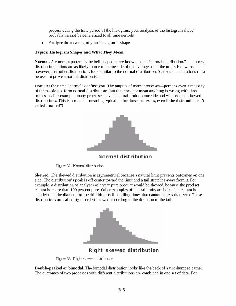
B-5

process during the time period of the histogram, your analysis of the histogram shape probably cannot be generalized to all time periods.

• Analyze the meaning of your histogram’s shape.

Typical Histogram Shapes and What They Mean

Normal. A common pattern is the bell-shaped curve known as the “normal distribution.” In a normal distribution, points are as likely to occur on one side of the average as on the other. Be aware, however, that other distributions look similar to the normal distribution. Statistical calculations must be used to prove a normal distribution.

Don’t let the name “normal” confuse you. The outputs of many processes—perhaps even a majority of them—do not form normal distributions, but that does not mean anything is wrong with those processes. For example, many processes have a natural limit on one side and will produce skewed distributions. This is normal — meaning typical — for those processes, even if the distribution isn’t called “normal”!

Figure 32. Normal distribution.

Skewed. The skewed distribution is asymmetrical because a natural limit prevents outcomes on one side. The distribution’s peak is off center toward the limit and a tail stretches away from it. For example, a distribution of analyses of a very pure product would be skewed, because the product cannot be more than 100 percent pure. Other examples of natural limits are holes that cannot be smaller than the diameter of the drill bit or call-handling times that cannot be less than zero. These distributions are called right- or left-skewed according to the direction of the tail.

Figure 33. Right-skewed distribution

Double-peaked or bimodal. The bimodal distribution looks like the back of a two-humped camel. The outcomes of two processes with different distributions are combined in one set of data. For

B-6

example, a distribution of production data from a two-shift operation might be bimodal, if each shift produces a different distribution of results. Stratification often reveals this problem.

Figure 34. Bimodal (double-peaked) distribution.

Plateau. The plateau might be called a “multimodal distribution.” Several processes with normal distributions are combined. Because there are many peaks close together, the top of the distribution resembles a plateau.

Figure 35. Plateau distribution.

Edge peak. The edge peak distribution looks like the normal distribution except that it has a large peak at one tail. Usually this is caused by faulty construction of the histogram, with data lumped together into a group labeled “greater than…”

Figure 36. Edge peak distribution.

Truncated or heart-cut. The truncated distribution looks like a normal distribution with the tails cut off. The supplier might be producing a normal distribution of material and then relying on inspection to separate what is within specification limits from what is out of spec. The resulting shipments to the customer from inside the specifications are the heart cut.

B-7

Figure 37. Truncated or heart-cut distribution.

B.4 Pareto Chart

Also called: Pareto diagram, Pareto analysis

Variations: weighted Pareto chart, comparative Pareto charts

Description

A Pareto chart is a bar graph. The lengths of the bars represent frequency or cost (time or money), and are arranged with the longest bars on the left and the shortest to the right. In this way the chart visually depicts which situations are more significant.

When to Use

• When analyzing data about the frequency of problems or causes in a process. This would be best used when evaluating the repeated engineering changes to fix a problem or documentation that was not done properly in the first engineering change processed.

• When there are many problems or causes and you want to focus on the most significant.

• When analyzing broad causes by looking at their specific components.

• When communicating with others about your data.

Process

1. Decide what categories you will use to group items.

2. Decide what measurement is appropriate. Common measurements are frequency, quantity, cost and time.

3. Decide what period of time the chart will cover: One work cycle? One full day? A week?

4. Collect the data, recording the category each time. (Or assemble data that already exist).

5. Subtotal the measurements for each category.

6. Determine the appropriate scale for the measurements you have collected. The maximum value will be the largest subtotal from step 5. (If you will do optional steps 8 and 9 below, the maximum value will be the sum of all subtotals from step 5). Mark the scale on the left side of the chart.

7. Construct and label bars for each category. Place the tallest at the far left, then the next tallest to its right and so on. If there are many categories with small measurements, they can be grouped as “other.”

B-8

- Steps 8 and 9 are optional but are useful for analysis and communication.

8. Calculate the percentage for each category: the subtotal for that category divided by the total for all categories. Draw a right vertical axis and label it with percentages. Be sure the two scales match: For example, the left measurement that corresponds to one-half should be exactly opposite 50% on the right scale.

9. Calculate and draw cumulative sums: Add the subtotals for the first and second categories, and place a dot above the second bar indicating that sum. To that sum add the subtotal for the third category, and place a dot above the third bar for that new sum. Continue the process for all the bars. Connect the dots, starting at the top of the first bar. The last dot should reach 100 percent on the right scale.

Example

Figure 38 shows how many customer complaints were received in each of five categories.

Figure 39 takes the largest category; “documents,” from the first Pareto diagram breaks it down into six categories of document-related complaints, and shows cumulative values.

If all complaints cause equal distress to the customer, working on eliminating document-related complaints would have the most impact, and of those, working on quality certificates should be most fruitful.

Figure 38. Customer complaints pareto.

B-9

Figure 39. Document complaints pareto.

B.5 Scatter Diagram

For the arrows shown in Figure 40, a Scatter Diagram is used when it is suspected that the variation of two items is connected in some way, to show any actual correlation between the two. Use it when it is suspected that one item may be causing another, to build evidence for the connection between the two. Use it only when both items being measured can be measured together, in pairs.

Figure 40. Examples of where scatter diagrams are used.

When investigating problems, typically when searching for their causes, it may be suspected that two items are related in some way. For example, it may be suspected that the number of accidents at work is related to the amount of overtime that people are working.

The Scatter Diagram helps to identify the existence of a measurable relationship between two such items by measuring them in pairs and plotting them on a graph, as shown on Figure 41 below. This visually shows the correlation between the two sets of measurements.

B-10

Figure 41. Points on scatter diagram.

If the points plotted on the Scatter Diagram are randomly scattered, with no discernible pattern, then this indicates that the two sets of measurements have no correlation and cannot be said to be related in any way. If, however, the points form a pattern of some kind, then this shows the type of relationship between the two measurement sets.

A Scatter Diagram shows correlation between two items for three reasons:

1. There is a cause and effect relationship between the two measured items, where one is causing the other (at least in part).

2. The two measured items are both caused by a third item. For example, a Scatter Diagram which shows a correlation between cracks and transparency of glass utensils because changes in both are caused by changes in furnace temperature.

3. Complete coincidence. It is possible to find high correlation of unrelated items, such as the number of ants crossing a path and newspaper sales.

Scatter Diagrams may thus be used to give evidence for a cause and effect relationship, but they alone do not prove it. Usually, it also requires a good understanding of the system being measured, and may require additional experiments. ‘Cause’ and ‘effect’ are thus quoted to indicate that although they may be suspected of having this relationship, it is not certain.

When evaluating a Scatter Diagram, both the degree and type of correlation should be considered. The visible differences in Scatter Diagrams for these are shown in Figures 43 and 44 below.

Where there is a cause-effect relationship, the degree of scatter in the diagram may be affected by several factors (as illustrated in the Figure 42 below):

• The proximity of the cause and effect. There is better chance of a high correlation if the cause is directly connected to the effect than if it is at the end of a chain of causes. Thus a root cause may not have a clear relationship with the end effect.

B-11

• Multiple causes of the effect. When measuring one cause, other causes are making the effect vary in an unrelated way. Other causes may also be having a greater effect, swamping the actual effect of the cause in question.

• Natural variation in the system. The effect may not react in the same way each time, even to a close major cause.

Figure 42. Scatter affected by several causes.

There is no one clear degree of correlation above which a clear relationship can be said to exist. Instead, as the degree of correlation increases, the probability of that relationship also increases.

If there is sufficient correlation, then the shape of the Scatter Diagram will indicate the type of correlation (see Figure 43 below). The most common shape is a straight line, either sloping up (positive correlation) or sloping down (negative correlation).

B-12

Scatter Diagram Degree of Correlation Interpretation

None No relationship can be seen. The ‘effect’ is not related to the ‘cause’ in any way.

Low A vague relationship is seen. The ‘cause’ may affect the ‘effect’, but only distantly. There are either more immediate causes to be found or there is significant variation in the ‘effect’.

High The points are grouped into a clear linear shape. It is probable that the ‘cause’ is directly related to the ‘effect’. Hence, any change in ‘cause’ will result in a reasonably predictable change in ‘effect’.

Perfect All points lie on a line (which is usually straight). Given any ‘cause’ value, the corresponding ‘effect’ value can be predicted with complete certainty.

Figure 43. Degrees of correlation.

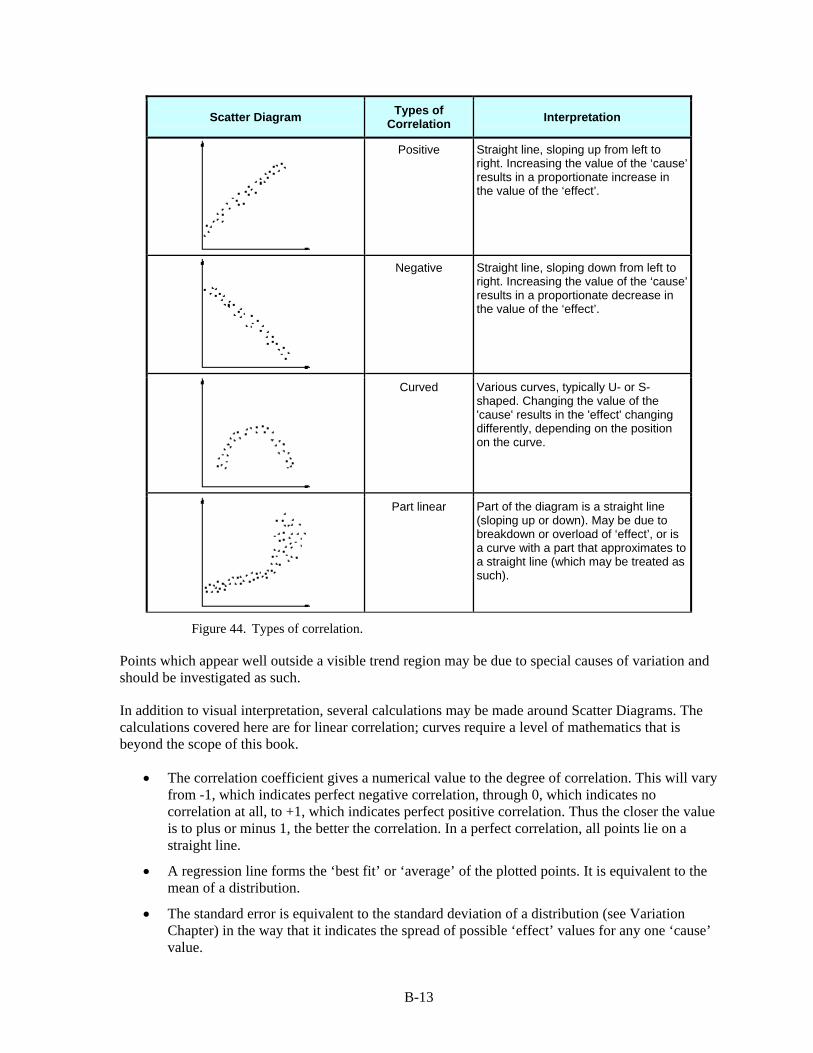
B-13

Scatter Diagram Types of Correlation Interpretation

Positive Straight line, sloping up from left to right. Increasing the value of the ‘cause’ results in a proportionate increase in the value of the ‘effect’.

Negative Straight line, sloping down from left to right. Increasing the value of the ‘cause’ results in a proportionate decrease in the value of the ‘effect’.

Curved Various curves, typically U- or S-shaped. Changing the value of the 'cause' results in the 'effect' changing differently, depending on the position on the curve.

Part linear Part of the diagram is a straight line (sloping up or down). May be due to breakdown or overload of ‘effect’, or is a curve with a part that approximates to a straight line (which may be treated as such).

Figure 44. Types of correlation.

Points which appear well outside a visible trend region may be due to special causes of variation and should be investigated as such.

In addition to visual interpretation, several calculations may be made around Scatter Diagrams. The calculations covered here are for linear correlation; curves require a level of mathematics that is beyond the scope of this book.

• The correlation coefficient gives a numerical value to the degree of correlation. This will vary from -1, which indicates perfect negative correlation, through 0, which indicates no correlation at all, to +1, which indicates perfect positive correlation. Thus the closer the value is to plus or minus 1, the better the correlation. In a perfect correlation, all points lie on a straight line.

• A regression line forms the ‘best fit’ or ‘average’ of the plotted points. It is equivalent to the mean of a distribution.

• The standard error is equivalent to the standard deviation of a distribution (see Variation Chapter) in the way that it indicates the spread of possible ‘effect’ values for any one ‘cause’ value.

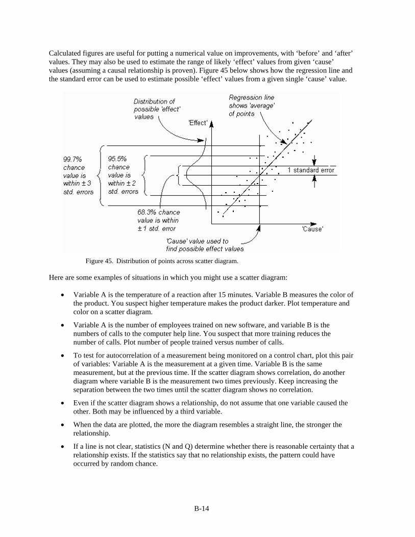
B-14

Calculated figures are useful for putting a numerical value on improvements, with ‘before’ and ‘after’ values. They may also be used to estimate the range of likely ‘effect’ values from given ‘cause’ values (assuming a causal relationship is proven). Figure 45 below shows how the regression line and the standard error can be used to estimate possible ‘effect’ values from a given single ‘cause’ value.

Figure 45. Distribution of points across scatter diagram.

Here are some examples of situations in which you might use a scatter diagram:

• Variable A is the temperature of a reaction after 15 minutes. Variable B measures the color of the product. You suspect higher temperature makes the product darker. Plot temperature and color on a scatter diagram.

• Variable A is the number of employees trained on new software, and variable B is the numbers of calls to the computer help line. You suspect that more training reduces the number of calls. Plot number of people trained versus number of calls.

• To test for autocorrelation of a measurement being monitored on a control chart, plot this pair of variables: Variable A is the measurement at a given time. Variable B is the same measurement, but at the previous time. If the scatter diagram shows correlation, do another diagram where variable B is the measurement two times previously. Keep increasing the separation between the two times until the scatter diagram shows no correlation.

• Even if the scatter diagram shows a relationship, do not assume that one variable caused the other. Both may be influenced by a third variable.

• When the data are plotted, the more the diagram resembles a straight line, the stronger the relationship.

• If a line is not clear, statistics (N and Q) determine whether there is reasonable certainty that a relationship exists. If the statistics say that no relationship exists, the pattern could have occurred by random chance.

B-15

• If the scatter diagram shows no relationship between the variables, consider whether the data might be stratified.

• If the diagram shows no relationship, consider whether the independent (x-axis) variable has been varied widely. Sometimes a relationship is not apparent because the data don’t cover a wide enough range.

• Think creatively about how to use scatter diagrams to discover a root cause.

• Drawing a scatter diagram is the first step in looking for a relationship between variables.

B.6 Stratification

Also called: flowchart or run chart

Description

Stratification is a technique used in combination with other data analysis tools. When data from a variety of sources or categories have been lumped together, the meaning of the data can be impossible to see. This technique separates the data so that patterns can be seen.

When to Use

• Before collecting data.

• When data come from several sources or conditions, such as shifts, days of the week, suppliers or population groups.

• When data analysis may require separating different sources or conditions.

Procedure

1. Before collecting data, consider which information about the sources of the data might have an effect on the results. Set up the data collection so that you collect that information as well.

2. When plotting or graphing the collected data on a scatter diagram, control chart, histogram or other analysis tool, use different marks or colors to distinguish data from various sources. Data that are distinguished in this way are said to be “stratified.”

3. Analyze the subsets of stratified data separately. For example, on a scatter diagram where data are stratified into data from source 1 and data from source 2, draw quadrants, count points and determine the critical value only for the data from source 1, then only for the data from source 2.

Example

The ZZ-400 manufacturing team drew a scatter diagram in Figure 46 to test whether product purity and iron contamination were related, but the plot did not demonstrate a relationship. Then a team member realized that the data came from three different reactors. The team member redrew the diagram, using a different symbol for each reactor’s data:

B-16

Figure 46. Purity vs iron stratification diagram.

Now patterns can be seen. The data from reactor 2 and reactor 3 are circled. Even without doing any calculations, it is clear that for those two reactors, purity decreases as iron increases. However, the data from reactor 1, the solid dots that are not circled, do not show that relationship. Something is different about reactor 1.

Considerations

Here are examples of different sources that might require data to be stratified:

• Equipment

• Shifts

• Departments

• Materials

• Suppliers

B-17

• Day of the week

• Time of day

• Products

• Survey data usually benefit from stratification.

• Always consider before collecting data whether stratification might be needed during analysis. Plan to collect stratification information. After the data are collected it might be too late.

• On your graph or chart, include a legend that identifies the marks or colors used.

B.7 Flowcharting

Also called: process flowchart, process flow diagram.

Variations: macro flowchart, top-down flowchart, detailed flowchart (also called process map, micro map, service map, or symbolic flowchart), deployment flowchart (also called down-across or cross-functional flowchart), several-leveled flowchart.

Description

A flowchart is a picture of the separate steps of a process in sequential order.

Elements that may be included are: sequence of actions, materials or services entering or leaving the process (inputs and outputs), decisions that must be made, people who become involved, time involved at each step and/or process measurements.

The process described can be anything: a manufacturing process, an administrative or service process, a project plan. This is a generic tool that can be adapted for a wide variety of purposes.

When to Use

• To develop understanding of how a process is done.

• To study a process for improvement.

• To communicate to others how a process is done.

• When better communication is needed between people involved with the same process.

• To document a process.

• When planning a project.

Basic Procedure

Materials needed: sticky notes or cards, a large piece of flipchart paper or newsprint, marking pens.

1. Define the process to be diagrammed. Write its title at the top of the work surface.

2. Discuss and decide on the boundaries of your process: Where or when does the process start? Where or when does it end? Discuss and decide on the level of detail to be included in the diagram.

B-18

3. Brainstorm the activities that take place. Write each on a card or sticky note. Sequence is not important at this point, although thinking in sequence may help people remember all the steps.

4. Arrange the activities in proper sequence.

5. When all activities are included and everyone agrees that the sequence is correct, draw arrows to show the flow of the process.

6. Review the flowchart with others involved in the process (workers, supervisors, and suppliers, customers) to see if they agree that the process is drawn accurately.

Considerations

Don’t worry too much about drawing the flowchart the “right way.” The right way is the way that helps those involved understand the process.

Identify and involve in the flowcharting process all key people involved with the process. This includes those who do the work in the process: suppliers, customers, and supervisors. Involve them in the actual flowcharting sessions by interviewing them before the sessions and/or by showing them the developing flowchart between work sessions and obtaining their feedback.

Do not assign a “technical expert” to draw the flowchart. People who actually perform the process should do it.

Computer software is available for drawing flowcharts. Software is useful for drawing a neat final diagram, but the method given here works better for the messy initial stages of creating the flowchart.

Examples:

Figure 47. High-level flowchart for an order-filling process.

B-19

Figure 48. Detailed flow chart example – filling an order.

C-1

Appendix C. Data Analysis Approaches

C.1 Decision Matrix

Also called: Pugh matrix, decision grid, selection matrix or grid, problem matrix, problem selection matrix, opportunity analysis, solution matrix, criteria rating form, criteria-based matrix.

Description

A decision matrix evaluates and prioritizes a list of options. The team first establishes a list of weighted criteria and then evaluates each option against those criteria. This is a variation of the L-shaped matrix.

When to Use

• When a list of options must be narrowed to one choice.

• When the decision must be made on the basis of several criteria.

• After the list of options has been reduced to a manageable number by list reduction.

• Typical situations are:

- When one improvement opportunity or problem must be selected to work on.

- When only one solution or problem-solving approach can be implemented.

- When only one new product can be developed.

Procedure

1. Brainstorm the evaluation criteria appropriate to the situation. If possible, involve customers in this process.

2. Discuss and refine the list of criteria. Identify any criteria that must be included and any that must not be included. Reduce the list of criteria to those that the team believes are most important. Tools such as list reduction and multi-voting may be useful here.

3. Assign a relative weight to each criterion; based on how important that criterion is to the situation. Do this by distributing 10 points among the criteria. The assignment can be done by discussion and consensus. Or each member can assign weights, then the numbers for each criterion are added for a composite team weighting.

4. Draw an L-shaped matrix. Write the criteria and their weights as labels along one edge and the list of options along the other edge. Usually, whichever group has fewer items occupies the vertical edge.

5. Evaluate each choice against the criteria. There are three ways to do this:

Method 1: Establish a rating scale for each criterion. Some options are:

1, 2, 3: 1 = slight extent, 2 = some extent, 3 = great extent 1, 2, 3: 1 = low, 2 = medium, 3 = high 1, 2, 3, 4, 5: 1 = little to 5 = great 1, 4, 9: 1 = low, 4 = moderate, 9 = high

C-2

Make sure that your rating scales are consistent. Word your criteria and set the scales so that the high end of the scale (5 or 3) is always the rating that would tend to make you select that option: most impact on customers, greatest importance, least difficulty, greatest likelihood of success.

Method 2: For each criterion, rank-order all options according to how well each meets the criterion. Number them with 1 being the option that is least desirable according to that criterion.

Method 3: Pugh matrix: Establish a baseline, which may be one of the alternatives of the current product or service. For each criterion, rate each other alternative in comparison to the baseline, using scores of worse (–1), same (0), or better (+1). Finer rating scales can be used, such as 2, 1, 0, –1, –2 for a five-point scale or 3, 2, 1, 0, –1, –2, –3 for a seven-point scale. Again, be sure that positive numbers reflect desirable ratings.

Multiply each option’s rating by the weight. Add the points for each option. The option with the highest score will not necessarily be the one to choose, but the relative scores can generate meaningful discussion and lead the team toward consensus

Example

Figure 49 shows a decision matrix used by the customer service team at the Parisian Experience restaurant to decide which aspect of the overall problem of “long wait time” to tackle first. The problems they identified are customers waiting for the host, the waiter, the food, and the check.

The criteria they identified are “customer pain” (how much does this negatively affect the customer?), “ease to solve,” “effect on other systems,” and “speed to solve.” Originally, the criteria “ease to solve” was written as “difficulty to solve,” but that wording reversed the rating scale. With the current wording, a high rating on each criterion defines a state that would encourage selecting the problem: high customer pain, very easy to solve, high effect on other systems, and quick solution.

Figure 49. Decision matrix example.

C-3

“Customer pain” has been weighted with 5 points, showing that the team considers it by far the most important criterion, compared to 1 or 2 points for the others. The team chose a rating scale of high = 3, medium = 2, and low = 1. For example, let’s look at the problem “customers wait for food.” The customer pain is medium (2), because the restaurant ambiance is nice. This problem would not be easy to solve (low ease = 1), as it involves both waiters and kitchen staff. The effect on other systems is medium (2), because waiters have to make several trips to the kitchen. The problem will take a while to solve (low speed = 1), as the kitchen is cramped and inflexible. (Notice that this has forced a guess about the ultimate solution: kitchen redesign. This may or may not be a good guess.)

Each rating is multiplied by the weight for that criterion. For example, “customer pain” (weight of 5) for “customers wait for host” rates high (3) for a score of 15. The scores are added across the rows to obtain a total for each problem. “Customers wait for host” has the highest score at 28. Since the next highest score is 18, the host problem probably should be addressed first.

Considerations

A very long list of options can first be shortened with a tool such as list reduction or multi-voting.

Criteria that are often used fall under the general categories of effectiveness, feasibility, capability, cost, time required, support or enthusiasm (of team and of others). Here are other commonly used criteria:

For selecting a problem or an improvement opportunity:

• Within control of the team

• Financial payback

• Resources required (for example; money and people)

• Customer pain caused by the problem

• Urgency of problem

• Team interest or buy-in

• Effect on other systems

• Management interest or support

• Difficulty of solving

• Time required to solve.

• For selecting a solution:

• Root causes addressed by this solution

• Extent of resolution of problem

• Cost to implement (for example, money and time)

• Return on investment; availability of resources (people, time)

• Ease of implementation

• Time until solution is fully implemented

• Cost to maintain (for example, money and time)

C-4

• Ease of maintenance

• Support or opposition to the solution

• Enthusiasm by team members

• Team control of the solution

• Safety, health, or environmental factors

• Training factors

• Potential effects on other systems

• Potential effects on customers or suppliers

• Value to customer

• Problems during implementation

• Potential negative consequences.

This matrix can be used to compare opinions. When possible, however, it is better used to summarize data that have been collected about the various criteria.

Sub-teams can be formed to collect data on the various criteria.

Several criteria for selecting a problem or improvement opportunity require guesses about the ultimate solution. For example: evaluating resources required, payback, difficulty to solve, and time required to solve. Therefore, your rating of the options will only be as good as your assumptions about the solutions.

It’s critical that the high end of the criteria scale (5 or 3) always is the end you would want to choose. Criteria such as cost, resource use, and difficulty can cause mix-ups: low cost is highly desirable. If your rating scale sometimes rates a desirable state as 5 and sometimes as 1, you will not get correct results. You can avoid this by rewording your criteria: Say “low cost” instead of “cost”; “ease” instead of “difficulty.” Or, in the matrix column headings, write what generates low and high ratings. For example:

Importance Cost Difficulty low = 1 high = 5 high = 1 low = 5 high = 1 low = 5

When evaluating options by method 1, some people prefer to think about just one option, rating each criterion in turn across the whole matrix, and then doing the next option and so on. Others prefer to think about one criterion, working down the matrix for all options, then going on to the next criterion. Take your pick.

If individuals on the team assign different ratings to the same criterion, discuss this so people can learn from each other’s views and arrive at a consensus. Do not average the ratings or vote for the most popular one.

In some versions of this tool, the sum of the unweighted scores is also calculated and both totals are studied for guidance toward a decision.

When this tool is used to choose a plan, solution, or new product, results can be used to improve options. An option that ranks highly overall but has low scores on criteria A and B can be modified

C-5

with ideas from options that score well on A and B. This combining and improving can be done for every option, and then the decision matrix used again to evaluate the new options.

C.2 Multi-voting

Also called: NGT voting, nominal prioritization

Variations: sticking dots, weighted voting, multiple picking-out method (MPM)

Description

Multivoting narrows a large list of possibilities to a smaller list of the top priorities or to a final selection. Multivoting is preferable to straight voting because it allows an item that is favored by all, but not the top choice of any, to rise to the top.

When to Use

• After brainstorming or some other expansion tool has been used to generate a long list of possibilities.

• When the list must be narrowed down.

• When the decision must be made by group judgment.

Procedure

Materials needed: flipchart or whiteboard, marking pens, 5 to 10 slips of paper for each individual, pen or pencil for each individual.

Display the list of options. Combine duplicate items. Affinity diagrams can be useful to organize large numbers of ideas and eliminate duplication and overlap. List reduction may also be useful.

Number (or letter) all items.

Decide how many items must be on the final reduced list. Decide also how many choices each member will vote for. Usually, five choices are allowed. The longer the original list, the more votes will be allowed, up to 10.

Working individually, each member selects the five items (or whatever number of choices is allowed) he or she thinks most important. Then each member ranks the choices in order of priority, with the first choice ranking highest. For example, if each member has five votes, the top choice would be ranked five, the next choice four, and so on. Each choice is written on a separate paper, with the ranking underlined in the lower right corner.

Tally votes. Collect the papers, shuffle them, and then record on a flipchart or whiteboard. The easiest way to record votes is for the scribe to write all the individual rankings next to each choice. For each item, the rankings are totaled next to the individual rankings.

If a decision is clear, stop here. Otherwise, continue with a brief discussion of the vote. The purpose of the discussion is to look at dramatic voting differences, such as an item that received both 5 and 1 rating, and avoid errors from incorrect information or understandings about the item. The discussion should not result in pressure on anyone to change their vote.

C-6

Repeat the voting process in steps 4 and 5. If greater decision-making accuracy is required, this voting may be done by weighting the relative importance of each choice on a scale of 1 to 10, with 10 being most important.

Example

A team had to develop a list of key customers to interview. First, team members brainstormed a list of possible names. Since they wanted representation of customers in three different departments, they divided the list into three groups. Within each group, they used multi-voting to identify four first-choice interviewees. This example shows the multi-voting for one department.

Fifteen of the brainstormed names were in that department. Each team member was allowed five votes, giving five points to the top choice, four to the second choice, and so on down to one point for the fifth choice. The votes and tally are shown in Figure 50. (The names are fictitious, and any resemblance to real individuals is strictly coincidental.) Although several of the choices emerge as agreed favorites, significant differences are indicated by the number of choices that have both high and low rankings. The team will discuss the options to ensure that everyone has the same information, and then vote again.

Figure 50. Multi-voting example.

Approved Electronically by:

Technical Peer Review Performed by:

AEROSPACE REPORT NO.TOR-2014-02202


Russell E. Averill, GENERALMANAGERSPACE BASEDSURVEILLANCE DIVISIONSPACE PROGRAMOPERATIONS

Jacqueline M. Wyrwitzke,PRINC DIRECTORMISSION ASSURANCESUBDIVISIONSYSTEMS ENGINEERINGDIVISIONENGINEERING &TECHNOLOGY GROUP

Manuel De Ponte, SR VPNATL SYSNATIONAL SYSTEMSGROUP

Jackie M. Webb-Larkin,SECURITY SPECIALIST IIIGOVERNMENT SECURITYSECURITY OPERATIONSOPERATIONS & SUPPORTGROUP

Norman Y. Lao, DIRECTOR DEPTACQ RISK & RELIABILITY ENGINEERINGDEPTMISSION ASSURANCE SUBDIVISIONENGINEERING & TECHNOLOGY GROUP

Jacqueline M. Wyrwitzke, PRINC DIRECTORMISSION ASSURANCE SUBDIVISIONSYSTEMS ENGINEERING DIVISIONENGINEERING & TECHNOLOGY GROUP

© The Aerospace Corporation, 2014.

All trademarks, service marks, and trade names are the property of their respective owners.

SK0673

External Distribution

REPORT TITLE


REPORT NO. PUBLICATION DATE SECURITY CLASSIFICATION

TOR-2014-02202 July 15, 2014 UNCLASSIFIED

Charles [email protected]

Carlo [email protected]

Andrew [email protected]

David [email protected]

Robert [email protected]

Scott [email protected]

Aaron [email protected]

Chic [email protected]

Brent [email protected]

Larry [email protected]

Ken [email protected] Martin

Dean [email protected]

Mark [email protected]

Lisa [email protected] Dynamics

Glenn [email protected]


Theresa [email protected]

Barry [email protected]

Ruth [email protected] Grumman


Silvia [email protected] Grumman

Wayne [email protected] Launch

Christopher [email protected]

Alexis [email protected]

Thomas [email protected]

Edward [email protected] Grumman

Tim [email protected] Martin

Kevin [email protected] Inc

Larry [email protected] Martin

Will [email protected]

Shawn [email protected] Martin

Janica [email protected]

Brian [email protected]

Brad [email protected]

Jerald [email protected]

Bernie [email protected]

Jeff [email protected]

Kevin [email protected]

James [email protected] Grumman

Stephen [email protected] Launch

Shawn [email protected]

Louis D'Angelolouis.a.d'[email protected] Martin


Douglas [email protected]

Jaclyn [email protected]


Ken [email protected] MDA

Tom [email protected]

Mary D'[email protected]

Susanne [email protected] Grumman

David [email protected] Systems


Matt [email protected] Corporation

James [email protected]

Tracy [email protected]

Brad [email protected]

Sherri [email protected]

Richard [email protected]

Bruce [email protected] Grumman

Mike [email protected] Dynamics


Robert [email protected] Martin

Bill [email protected]

Jace [email protected]

Matteo [email protected]

Helen [email protected] Martin

Ricardo [email protected] Systems

Dale [email protected]

Chuck [email protected]

Luigi [email protected] Inc

Gregory [email protected]

Joe [email protected]

Lilian [email protected]

Harold [email protected]

Bob [email protected]

Frederick [email protected] Martin

Ben [email protected]

Rosemary [email protected] Machined


Paul [email protected] Martin


Eugene [email protected]

Dan [email protected] Grumman


Mike [email protected] Launch

Amanda [email protected]

Edward [email protected] Grumman

Jim [email protected]

Geoffrey [email protected] Electronics

Mike [email protected]

Yehwan [email protected]




Byron [email protected]

Hans [email protected]



John [email protected] Martin

Rick [email protected]

Steve [email protected]

Steve [email protected] Grumman

Louise [email protected]

C J [email protected]

Chris [email protected]


Eric [email protected]

Marvin [email protected]

Scott [email protected] Grumman

Don [email protected] Bearings

Scot [email protected] Martin

Sultan Ali [email protected] - Tech

Josh [email protected]

Henry [email protected] Systems

Art [email protected] Grumman



Lester [email protected]

Frank [email protected] Com

Joan [email protected]


Julio [email protected]

Kevin [email protected] Com

Miroslav [email protected] 51

John Mc [email protected]

Ian [email protected] Systems

Kurt [email protected]


Jo [email protected]

Charles [email protected] Martin

Edmond [email protected]

Dennis [email protected] Martin

George [email protected] Lubricants

Nancy [email protected] Batteries

Deanna [email protected]


John [email protected] Martin

Dave [email protected]

Ron [email protected]


Michael O'[email protected] Inc

Michael [email protected] Inc

Debra [email protected] Grumman


Anthony [email protected]

Joseph [email protected] Inc

Peter [email protected]


Paulette [email protected]


Steven [email protected]


Angela [email protected]

Dave [email protected]

Kay [email protected] Grumman

David [email protected] Systems

Forrest [email protected]


Bob [email protected] Grumman

Mike [email protected] Logic

Sally [email protected]

Troy [email protected] Microwave

Ralph [email protected]


John [email protected]

William [email protected]

Dennis [email protected] Grumman


Lane [email protected]

Michael [email protected]

Victor [email protected]

Don [email protected]

Fred [email protected] - Navy


Gerald [email protected]

Annie [email protected] Batteries


Tom [email protected] Corp

Jonathan [email protected]


Fredic [email protected]

Rob [email protected]


Melanie [email protected] Martin

Jerry [email protected] Martin

LaKeisha [email protected] Grumman

Jerry [email protected] Inc

Peter [email protected] Corp

Thomas [email protected] Grumman

George [email protected] Inc


Mauricio [email protected]

Jeffrey [email protected]

Bill [email protected] Grumman

Ghislain [email protected]

Deborah [email protected]

Fred Van [email protected]

Marvin [email protected]

Gerrit [email protected]


John [email protected] UTC

Vinvent [email protected]


John [email protected]

Brian [email protected] Allen Hamilton

Arthur [email protected] UTC

Craig [email protected] Grumman

Dan [email protected]


Charlie [email protected]



Mark [email protected] Grumman

Jian [email protected]

George [email protected]

APPROVED BY_________________________________________________________________ DATE_______________(AF OFFICE)

root cause investigation best practices guide of objectivity/incorrect problem definition: the team...

Documents