rotation matrix representations of orientation homogeneous ... · pdf filerotation matrix...
TRANSCRIPT
INDUSTRIAL ROBOTICS Prof. Bruno SICILIANO
KINEMATICS
• relationship between joint positions and end-effector positionand orientation
Rotation matrix
Representations of orientation
Homogeneous transformations
Direct kinematics
Joint space and operational space
Kinematic calibration
Inverse kinematics problem
INDUSTRIAL ROBOTICS Prof. Bruno SICILIANO
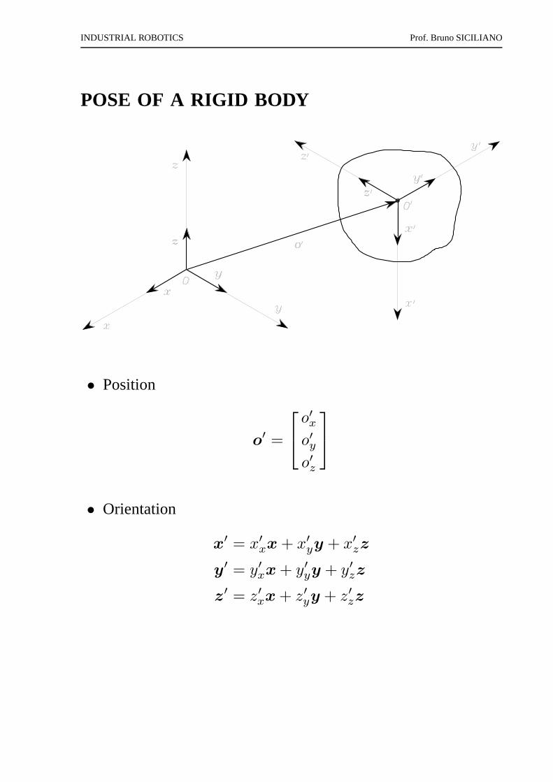
POSE OF A RIGID BODY
• Position
o′ =
o′xo′yo′z
• Orientation
x′ = x′xx + x′yy + x′zz
y′ = y′xx + y′yy + y′zz
z′ = z′xx + z′yy + z′zz
INDUSTRIAL ROBOTICS Prof. Bruno SICILIANO
ROTATION MATRIX
R =
x′ y′ z′
=
x′Tx y′Tx z′Tx
x′Ty y′Ty z′Ty
x′Tz y′Tz z′Tz
RTR = I
RT = R−1
INDUSTRIAL ROBOTICS Prof. Bruno SICILIANO
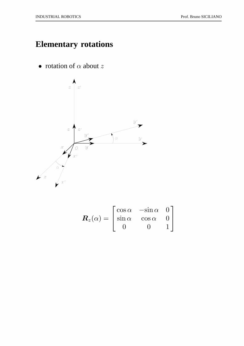
Elementary rotations
• rotation ofα aboutz
Rz(α) =
cosα −sinα 0sinα cosα 0
0 0 1
INDUSTRIAL ROBOTICS Prof. Bruno SICILIANO
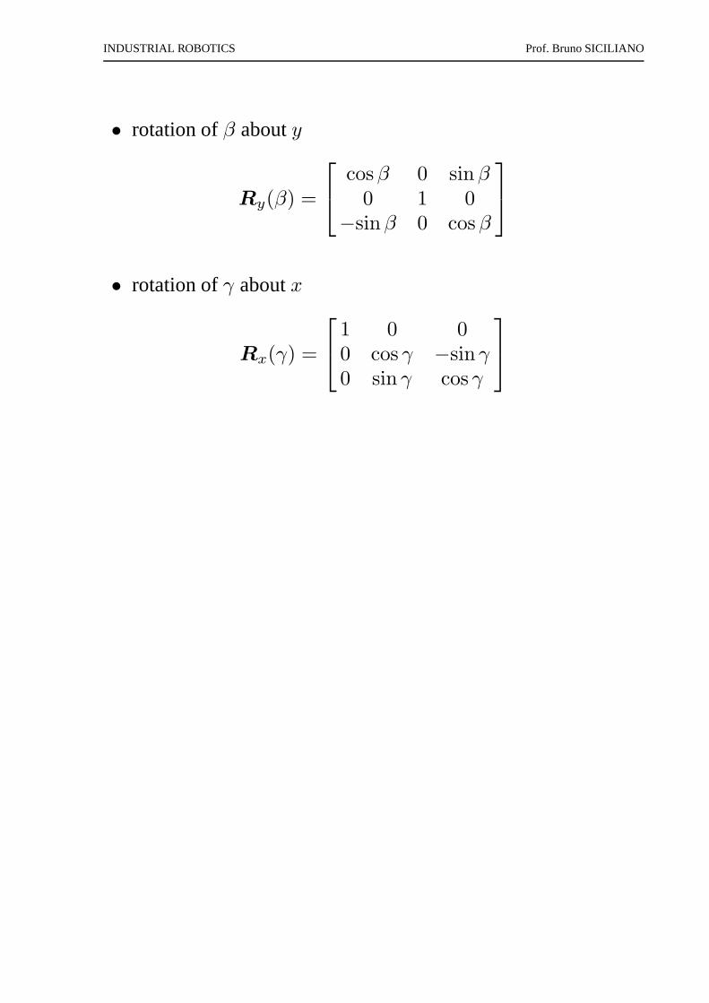
• rotation ofβ abouty
Ry(β) =
cosβ 0 sinβ0 1 0
−sinβ 0 cosβ
• rotation ofγ aboutx
Rx(γ) =
1 0 00 cos γ −sinγ0 sin γ cos γ
INDUSTRIAL ROBOTICS Prof. Bruno SICILIANO
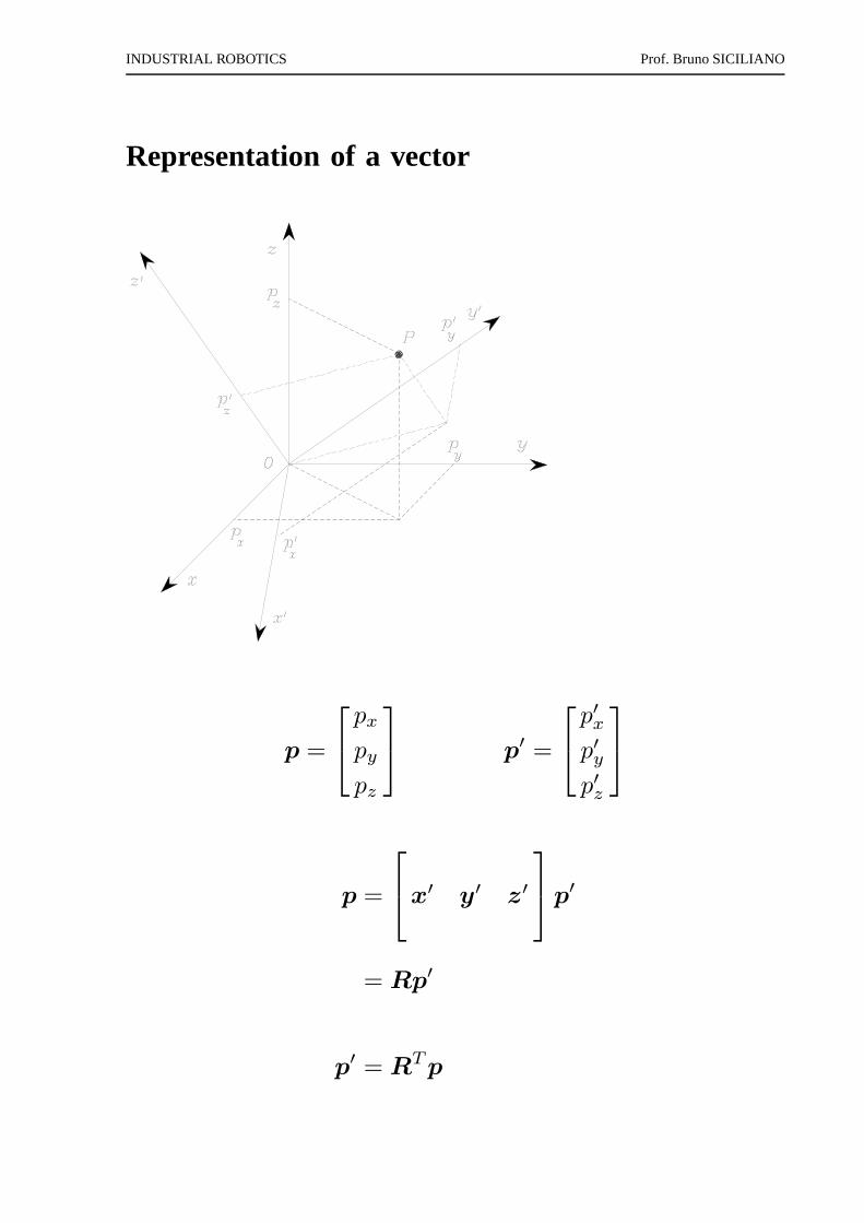
Representation of a vector
p =
pxpypz
p′ =
p′xp′yp′z
p =
x′ y′ z′
p′
= Rp′
p′ = RTp
INDUSTRIAL ROBOTICS Prof. Bruno SICILIANO
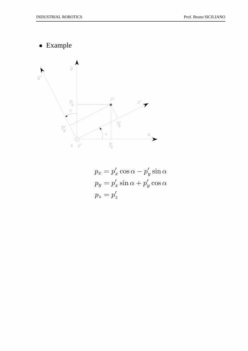
• Example
px = p′x cosα− p′y sinα
py = p′x sinα+ p′y cosα
pz = p′z
INDUSTRIAL ROBOTICS Prof. Bruno SICILIANO
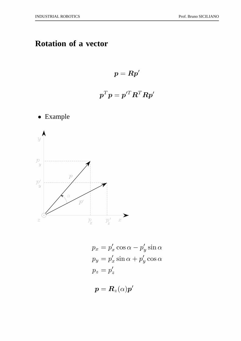
Rotation of a vector
p = Rp′
pTp = p′TRTRp′
• Example
px = p′x cosα− p′y sinα
py = p′x sinα+ p′y cosα
pz = p′z
p = Rz(α)p′
INDUSTRIAL ROBOTICS Prof. Bruno SICILIANO
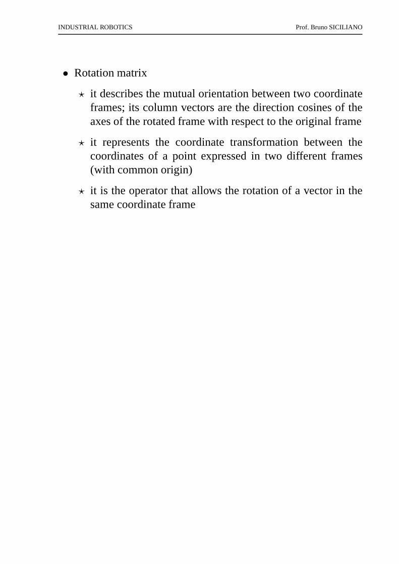
• Rotation matrix
⋆ it describes the mutual orientation between two coordinateframes; its column vectors are the direction cosines of theaxes of the rotated frame with respect to the original frame
⋆ it represents the coordinate transformation between thecoordinates of a point expressed in two different frames(with common origin)
⋆ it is the operator that allows the rotation of a vector in thesame coordinate frame
INDUSTRIAL ROBOTICS Prof. Bruno SICILIANO
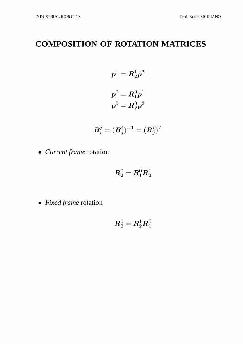
COMPOSITION OF ROTATION MATRICES
p1 = R12p
2
p0 = R01p
1
p0 = R02p
2
Rji = (Ri
j)−1 = (Ri
j)T
• Current frame rotation
R02 = R0
1R12
• Fixed frame rotation
R02 = R1
2R01
INDUSTRIAL ROBOTICS Prof. Bruno SICILIANO
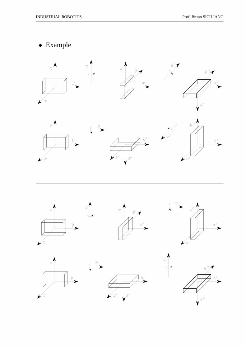
• Example

INDUSTRIAL ROBOTICS Prof. Bruno SICILIANO
EULER ANGLES
• rotation matrix
⋆ 9 parameters with 6 constraints
• minimal representation of orientation
⋆ 3 independent parameters
INDUSTRIAL ROBOTICS Prof. Bruno SICILIANO
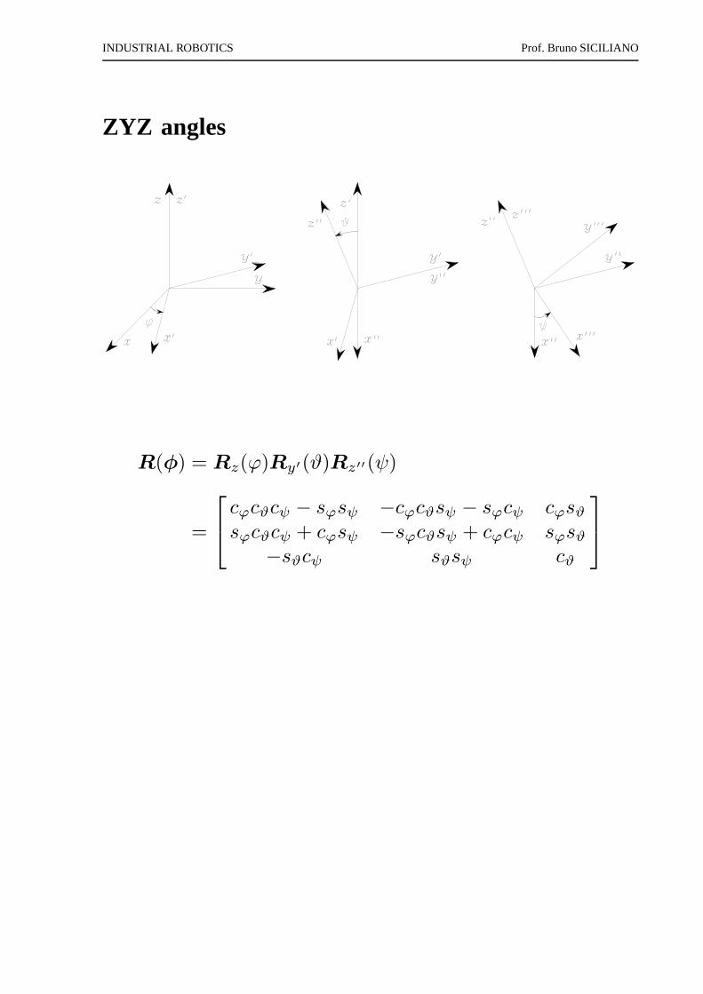
ZYZ angles
R(φ) = Rz(ϕ)Ry′(ϑ)Rz′′(ψ)
=
cϕcϑcψ − sϕsψ −cϕcϑsψ − sϕcψ cϕsϑsϕcϑcψ + cϕsψ −sϕcϑsψ + cϕcψ sϕsϑ
−sϑcψ sϑsψ cϑ
INDUSTRIAL ROBOTICS Prof. Bruno SICILIANO
• Inverse problem
⋆ Given
R =
r11 r12 r13r21 r22 r23r31 r32 r33
the three ZYZ angles are (ϑ ∈ (0, π))
ϕ = Atan2(r23, r13)
ϑ = Atan2
(
√
r213 + r223, r33
)
ψ = Atan2(r32,−r31)
or (ϑ ∈ (−π, 0))
ϕ = Atan2(−r23,−r13)
ϑ = Atan2
(
−√
r213 + r223, r33
)
ψ = Atan2(−r32, r31)
INDUSTRIAL ROBOTICS Prof. Bruno SICILIANO
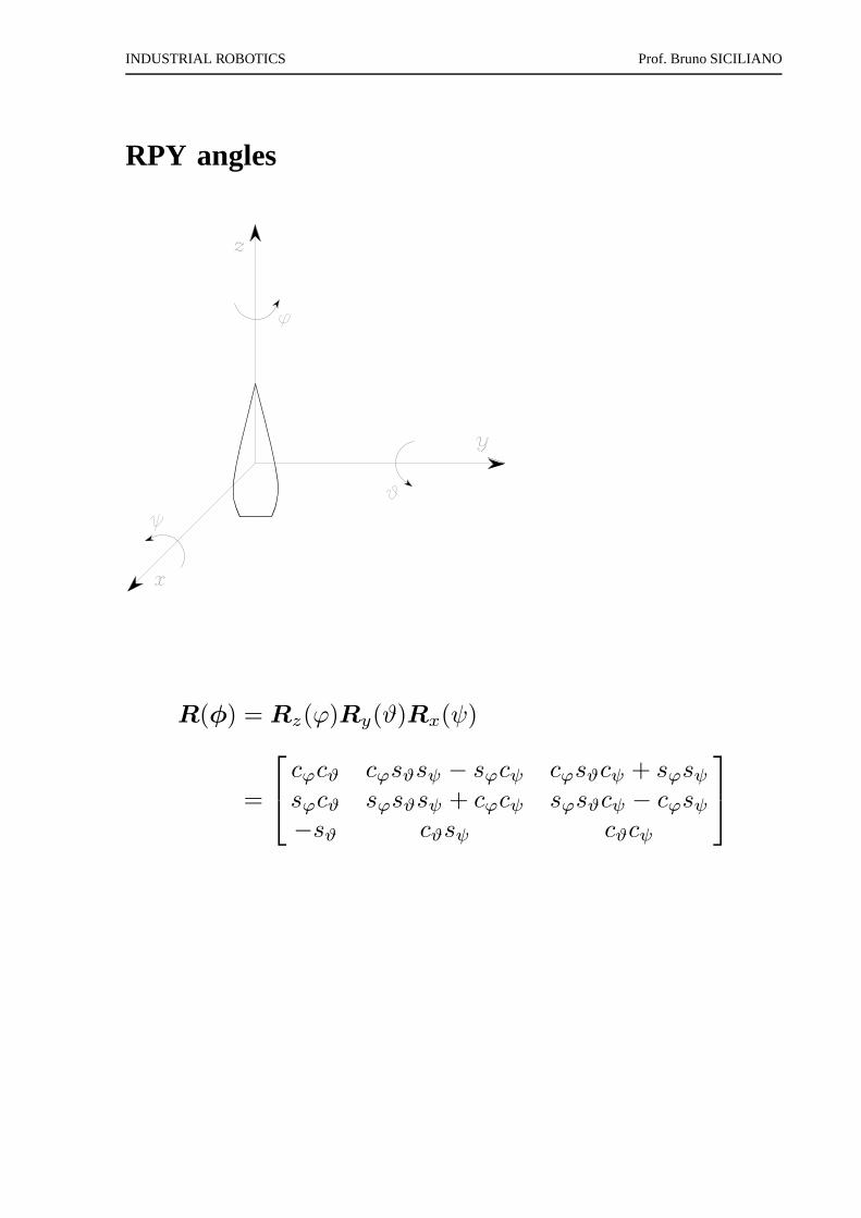
RPY angles
R(φ) = Rz(ϕ)Ry(ϑ)Rx(ψ)
=
cϕcϑ cϕsϑsψ − sϕcψ cϕsϑcψ + sϕsψsϕcϑ sϕsϑsψ + cϕcψ sϕsϑcψ − cϕsψ−sϑ cϑsψ cϑcψ
INDUSTRIAL ROBOTICS Prof. Bruno SICILIANO
• Inverse problem
⋆ Given
R =
r11 r12 r13r21 r22 r23r31 r32 r33
the three RPY angles are (ϑ ∈ (−π/2, π/2))
ϕ = Atan2(r21, r11)
ϑ = Atan2
(
−r31,√
r232 + r233
)
ψ = Atan2(r32, r33)
or (ϑ ∈ (π/2, 3π/2))
ϕ = Atan2(−r21,−r11)
ϑ = Atan2
(
−r31,−√
r232 + r233
)
ψ = Atan2(−r32,−r33)
INDUSTRIAL ROBOTICS Prof. Bruno SICILIANO
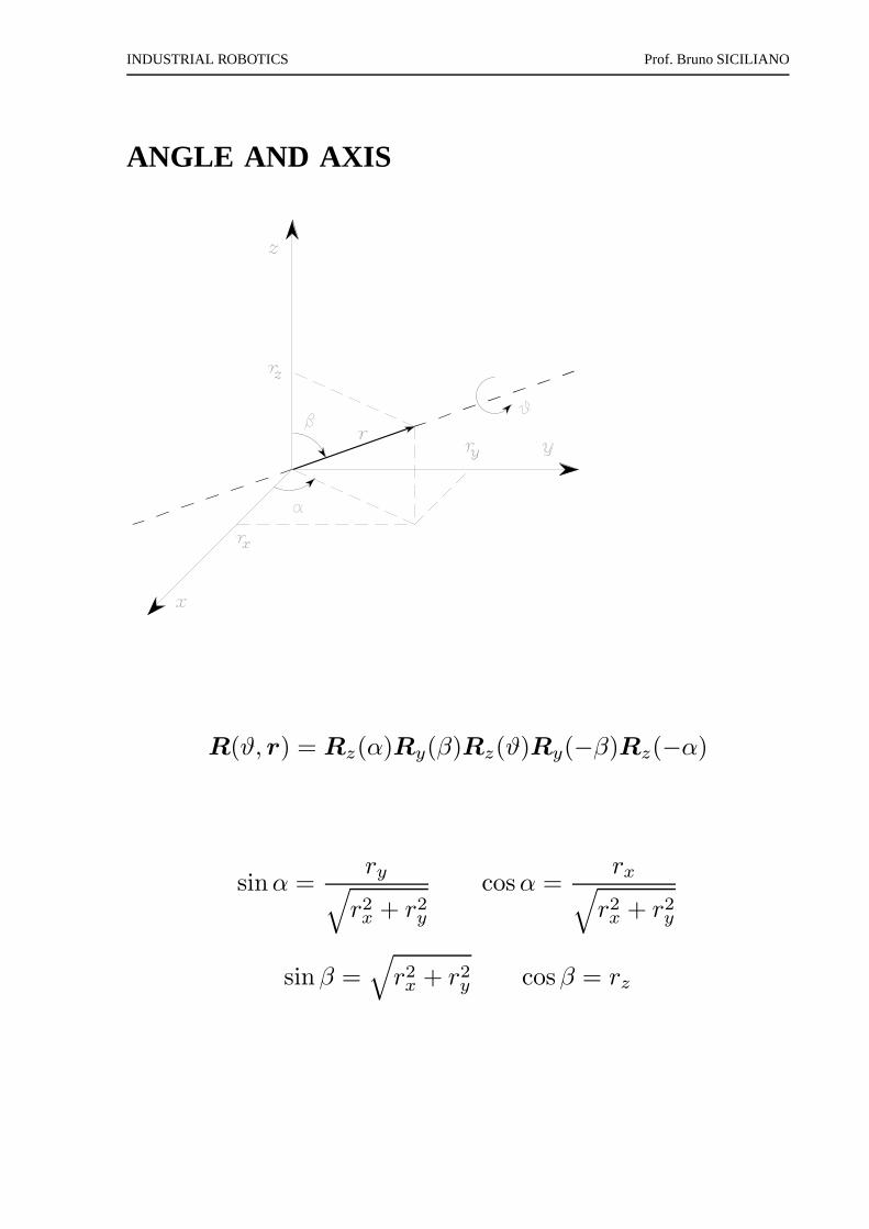
ANGLE AND AXIS
R(ϑ, r) = Rz(α)Ry(β)Rz(ϑ)Ry(−β)Rz(−α)
sinα =ry
√
r2x + r2y
cosα =rx
√
r2x + r2y
sinβ =√
r2x + r2y cosβ = rz
INDUSTRIAL ROBOTICS Prof. Bruno SICILIANO
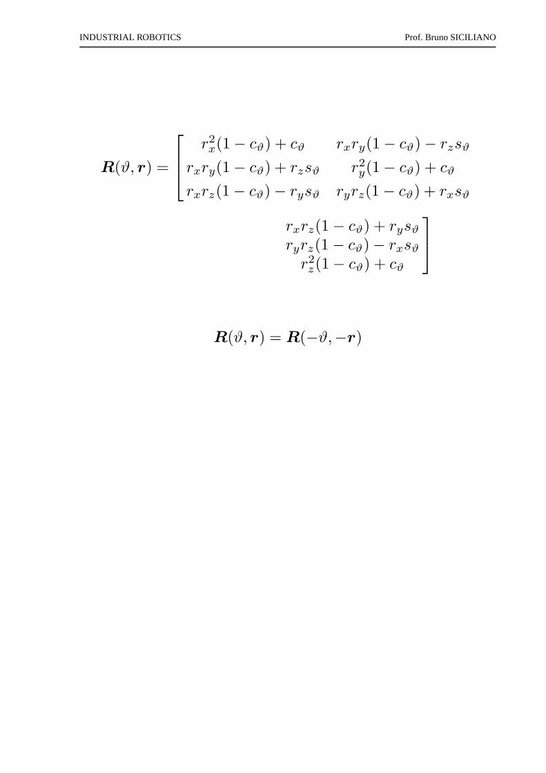
R(ϑ, r) =
r2x(1 − cϑ) + cϑ rxry(1 − cϑ) − rzsϑ
rxry(1 − cϑ) + rzsϑ r2y(1 − cϑ) + cϑ
rxrz(1 − cϑ) − rysϑ ryrz(1 − cϑ) + rxsϑ
rxrz(1 − cϑ) + rysϑryrz(1 − cϑ) − rxsϑr2z(1 − cϑ) + cϑ
R(ϑ, r) = R(−ϑ,−r)
INDUSTRIAL ROBOTICS Prof. Bruno SICILIANO
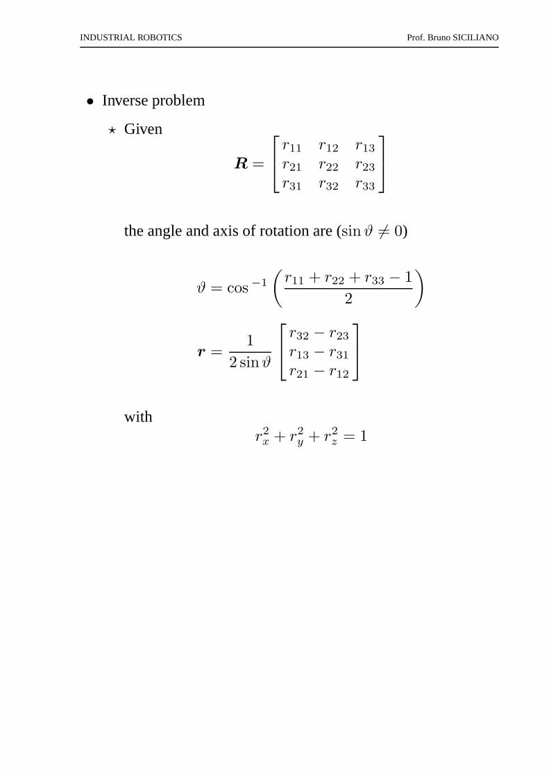
• Inverse problem
⋆ Given
R =
r11 r12 r13r21 r22 r23r31 r32 r33
the angle and axis of rotation are (sinϑ 6= 0)
ϑ = cos−1
(
r11 + r22 + r33 − 1
2
)
r =1
2 sinϑ
r32 − r23r13 − r31r21 − r12
withr2x + r2y + r2z = 1
INDUSTRIAL ROBOTICS Prof. Bruno SICILIANO
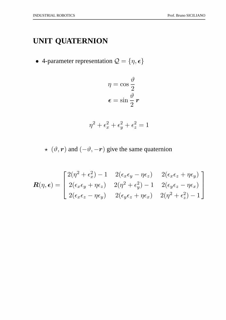
UNIT QUATERNION
• 4-parameter representationQ = {η, ǫ}
η = cosϑ
2
ǫ = sinϑ
2r
η2 + ǫ2x + ǫ2y + ǫ2z = 1
⋆ (ϑ, r) and(−ϑ,−r) give the same quaternion
R(η, ǫ) =
2(η2 + ǫ2x) − 1 2(ǫxǫy − ηǫz) 2(ǫxǫz + ηǫy)
2(ǫxǫy + ηǫz) 2(η2 + ǫ2y) − 1 2(ǫyǫz − ηǫx)
2(ǫxǫz − ηǫy) 2(ǫyǫz + ηǫx) 2(η2 + ǫ2z) − 1
INDUSTRIAL ROBOTICS Prof. Bruno SICILIANO
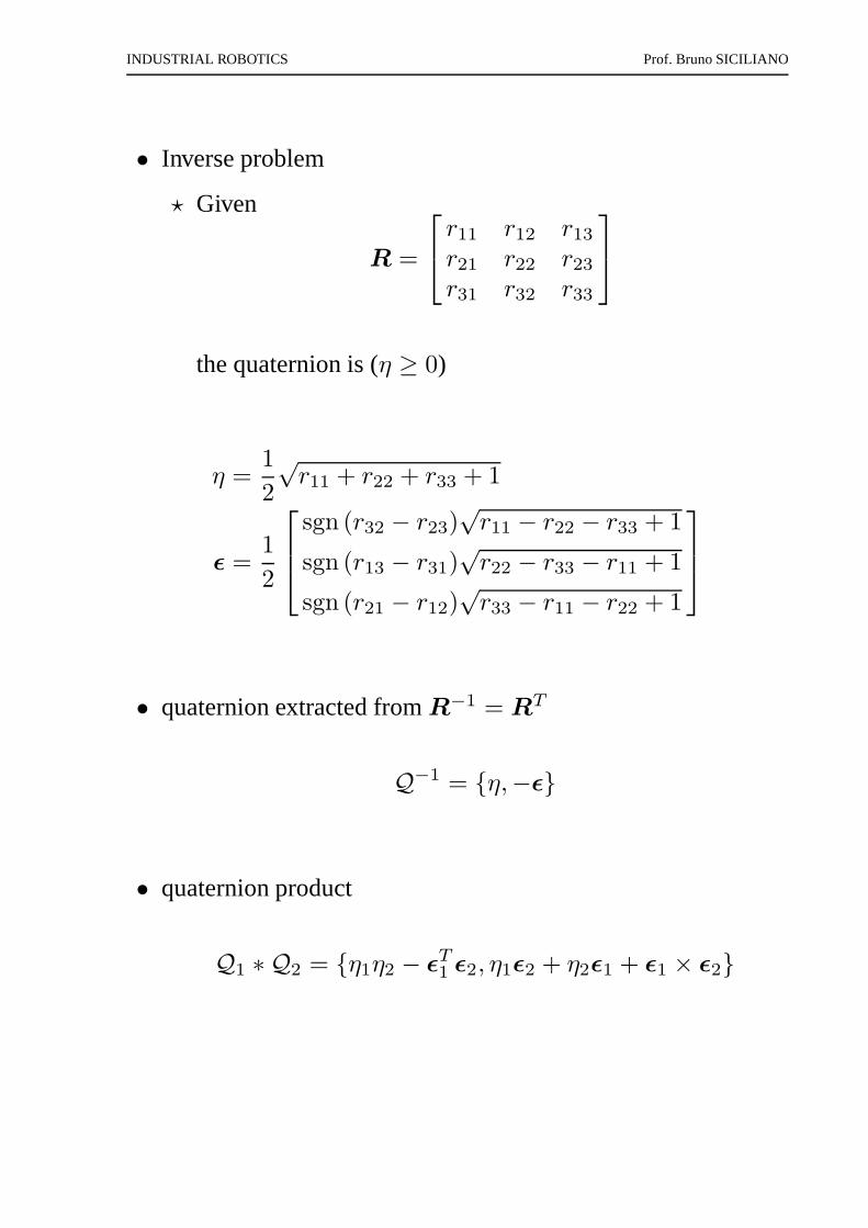
• Inverse problem
⋆ Given
R =
r11 r12 r13r21 r22 r23r31 r32 r33
the quaternion is (η ≥ 0)
η =1
2
√r11 + r22 + r33 + 1
ǫ =1
2
sgn (r32 − r23)√r11 − r22 − r33 + 1
sgn (r13 − r31)√r22 − r33 − r11 + 1
sgn (r21 − r12)√r33 − r11 − r22 + 1
• quaternion extracted fromR−1 = RT
Q−1 = {η,−ǫ}
• quaternion product
Q1 ∗ Q2 = {η1η2 − ǫT1 ǫ2, η1ǫ2 + η2ǫ1 + ǫ1 × ǫ2}
INDUSTRIAL ROBOTICS Prof. Bruno SICILIANO
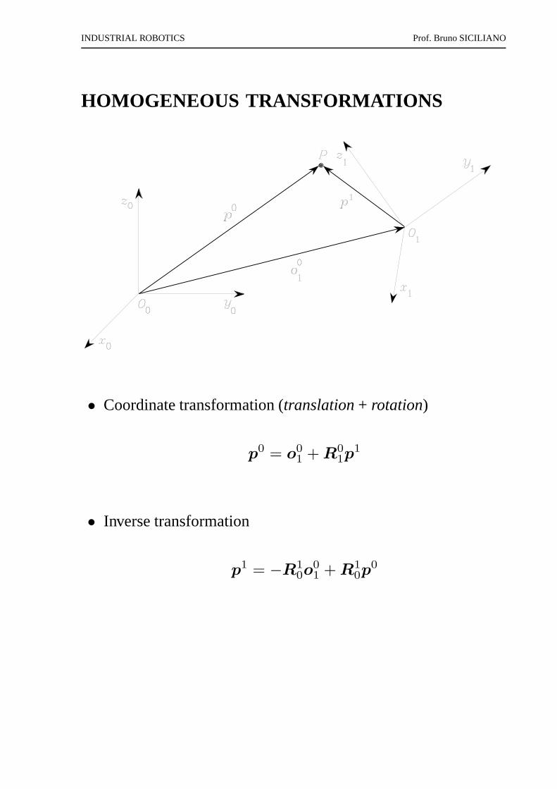
HOMOGENEOUS TRANSFORMATIONS
• Coordinate transformation (translation + rotation)
p0 = o01 + R0
1p1
• Inverse transformation
p1 = −R10o
01 + R1
0p0
INDUSTRIAL ROBOTICS Prof. Bruno SICILIANO
• Homogeneous representation
p̃ =
p
1
• Homogeneous transformation matrix
A01 =
R01 o0
1
0T 1
• Coordinate transformation
p̃0 = A01p̃
1
INDUSTRIAL ROBOTICS Prof. Bruno SICILIANO
• Inverse transformation
p̃1 = A10p̃
0 =(
A01
)−1p̃0
ove
A10 =
R10 −R1
0o01
0T 1
A−1 6= AT
• Sequence of coordinate transformations
p̃0 = A01A
12 . . .A
n−1n p̃n
INDUSTRIAL ROBOTICS Prof. Bruno SICILIANO
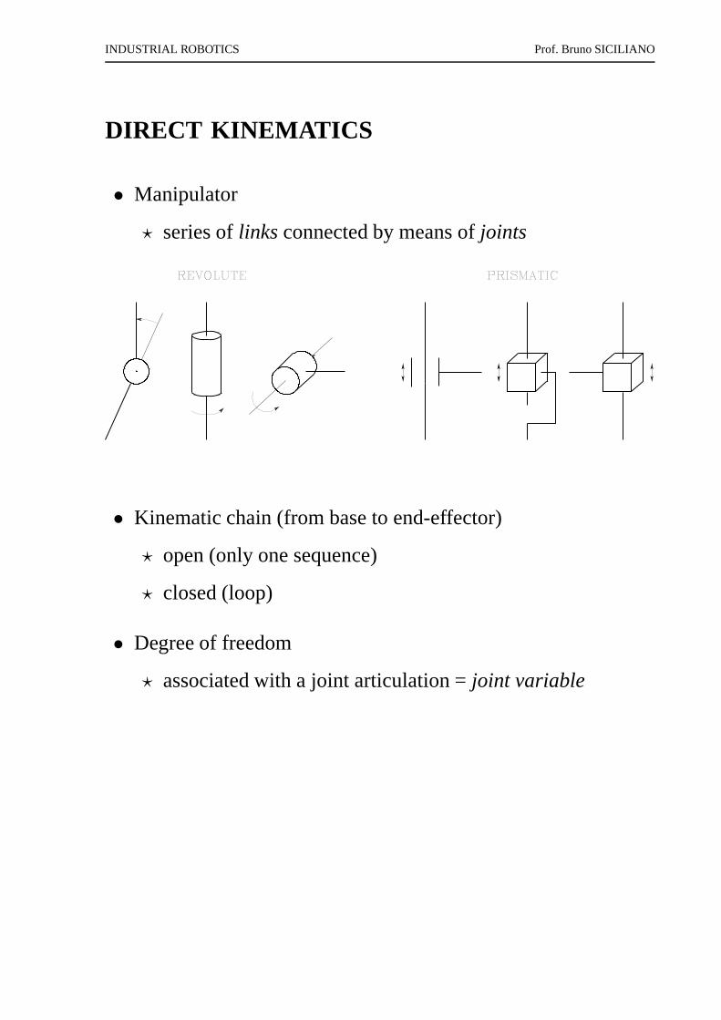
DIRECT KINEMATICS
• Manipulator
⋆ series oflinks connected by means ofjoints
• Kinematic chain (from base to end-effector)
⋆ open (only one sequence)
⋆ closed (loop)
• Degree of freedom
⋆ associated with a joint articulation =joint variable
INDUSTRIAL ROBOTICS Prof. Bruno SICILIANO
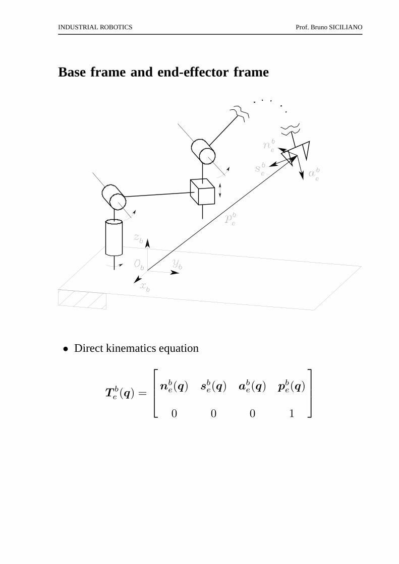
Base frame and end-effector frame
• Direct kinematics equation
T be (q) =
nbe(q) sbe(q) abe(q) pbe(q)
0 0 0 1
INDUSTRIAL ROBOTICS Prof. Bruno SICILIANO
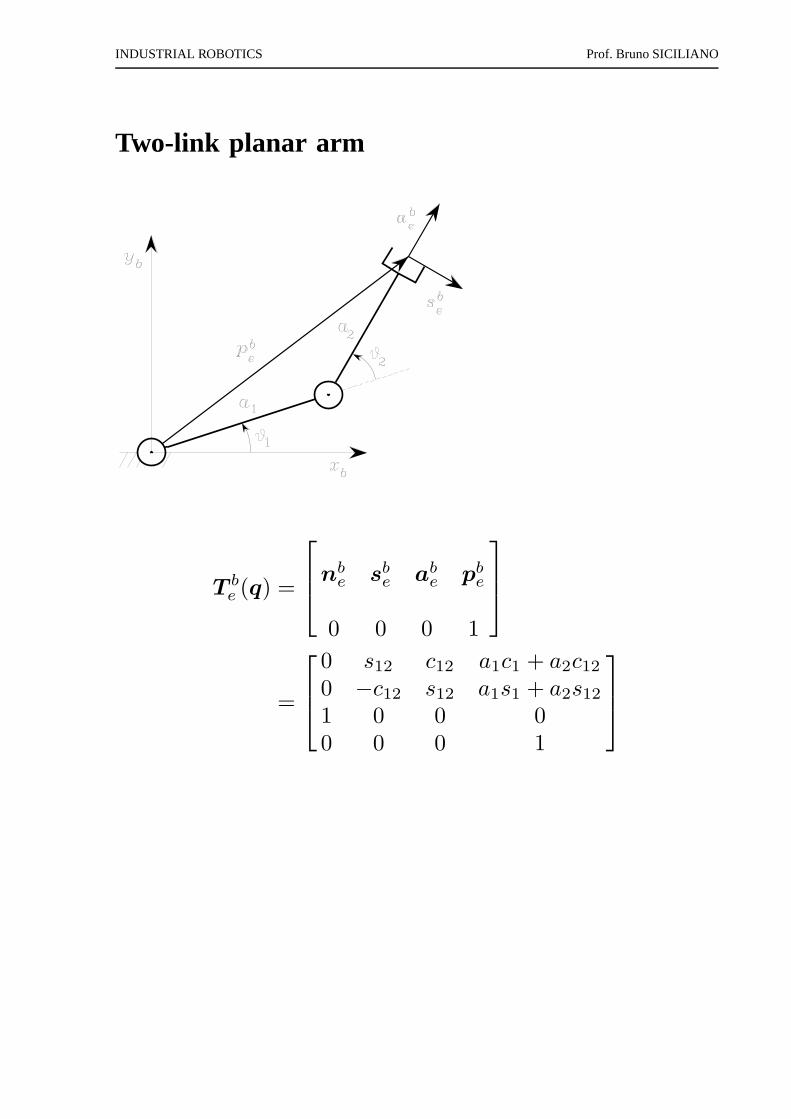
Two-link planar arm
T be (q) =
nbe sbe abe pbe
0 0 0 1
=
0 s12 c12 a1c1 + a2c120 −c12 s12 a1s1 + a2s121 0 0 00 0 0 1
INDUSTRIAL ROBOTICS Prof. Bruno SICILIANO
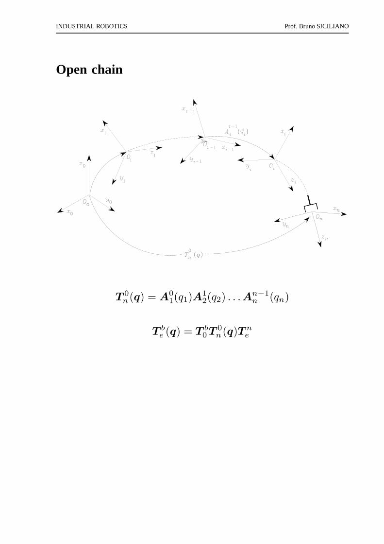
Open chain
T 0n (q) = A0
1(q1)A12(q2) . . .A
n−1n (qn)
T be (q) = T b
0 T 0n (q)T n
e
INDUSTRIAL ROBOTICS Prof. Bruno SICILIANO
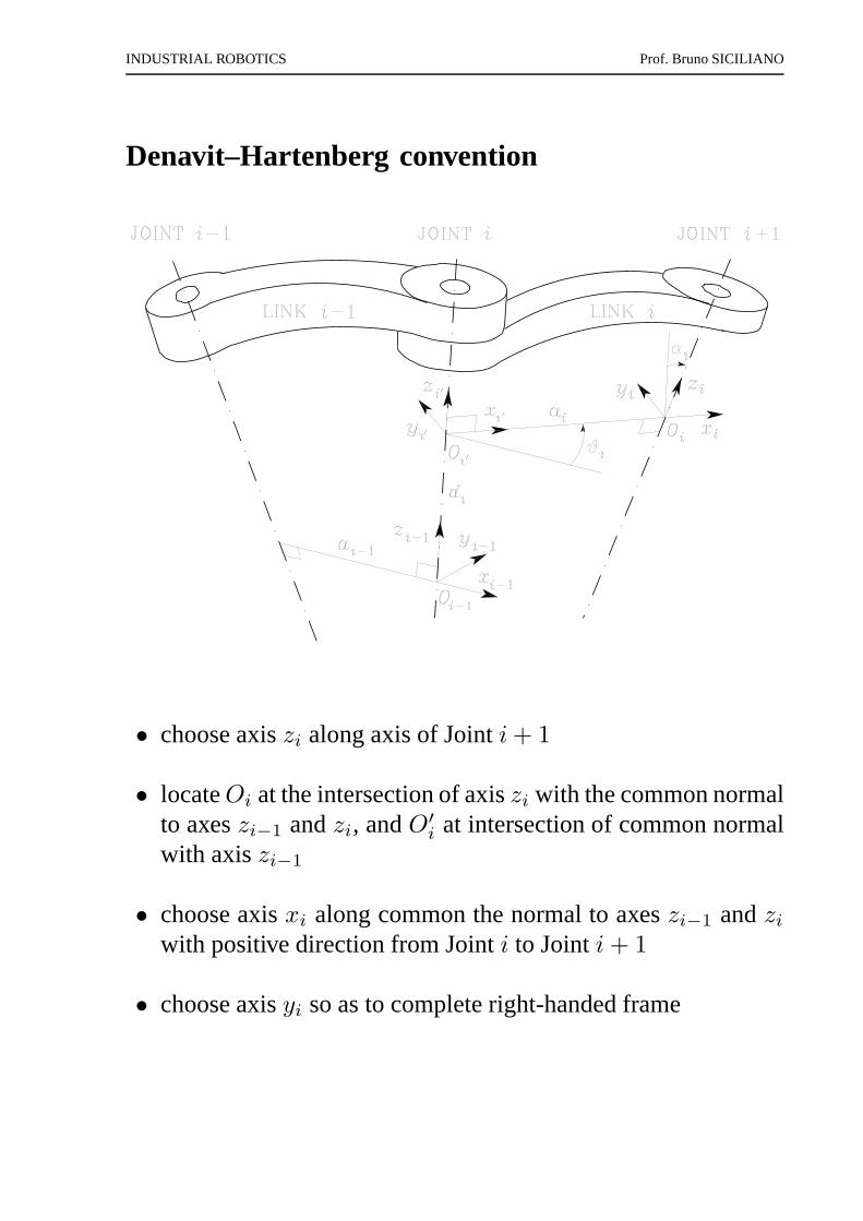
Denavit–Hartenberg convention
• choose axiszi along axis of Jointi+ 1
• locateOi at the intersection of axiszi with the common normalto axeszi−1 andzi, andO′
i at intersection of common normalwith axiszi−1
• choose axisxi along common the normal to axeszi−1 andziwith positive direction from Jointi to Jointi+ 1
• choose axisyi so as to complete right-handed frame
INDUSTRIAL ROBOTICS Prof. Bruno SICILIANO
• Nonunique definition of link frame:
⋆ for Frame0, only the direction of axisz0 is specified:thenO0 andx0 can be chosen arbitrarily
⋆ for Framen, since there is no Jointn+1, zn is not uniquelydefined whilexn has to be normal to axiszn−1); typicallyJointn is revolute and thuszn can be aligned withzn−1
⋆ when two consecutive axes are parallel, the common normalbetween them is not uniquely defined
⋆ when two consecutive axes intersect, the positive directionof xi is arbitrary
⋆ when Jointi is prismatic, only the direction ofzi−1 isspecified
INDUSTRIAL ROBOTICS Prof. Bruno SICILIANO
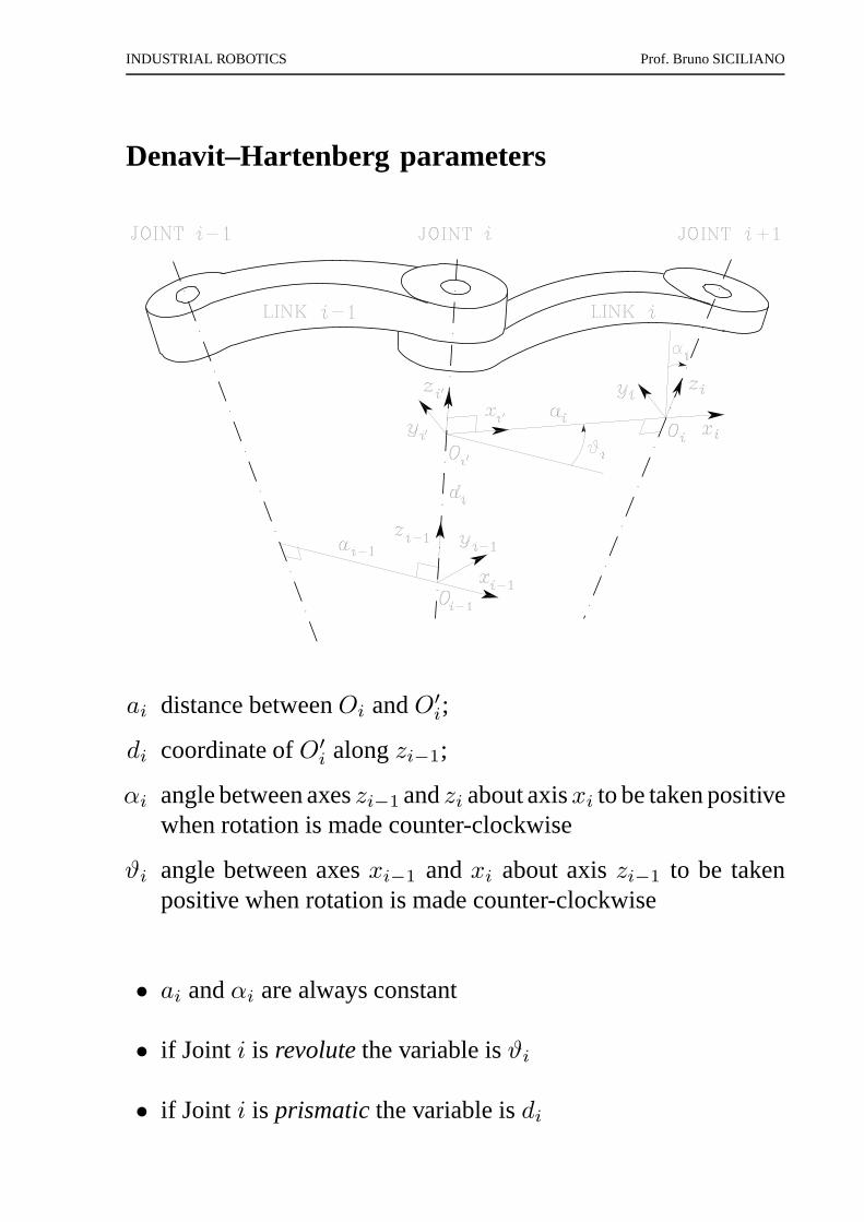
Denavit–Hartenberg parameters
ai distance betweenOi andO′
i;
di coordinate ofO′
i alongzi−1;
αi angle between axeszi−1 andzi about axisxi to be taken positivewhen rotation is made counter-clockwise
ϑi angle between axesxi−1 andxi about axiszi−1 to be takenpositive when rotation is made counter-clockwise
• ai andαi are always constant
• if Joint i is revolute the variable isϑi
• if Joint i is prismatic the variable isdi
INDUSTRIAL ROBOTICS Prof. Bruno SICILIANO
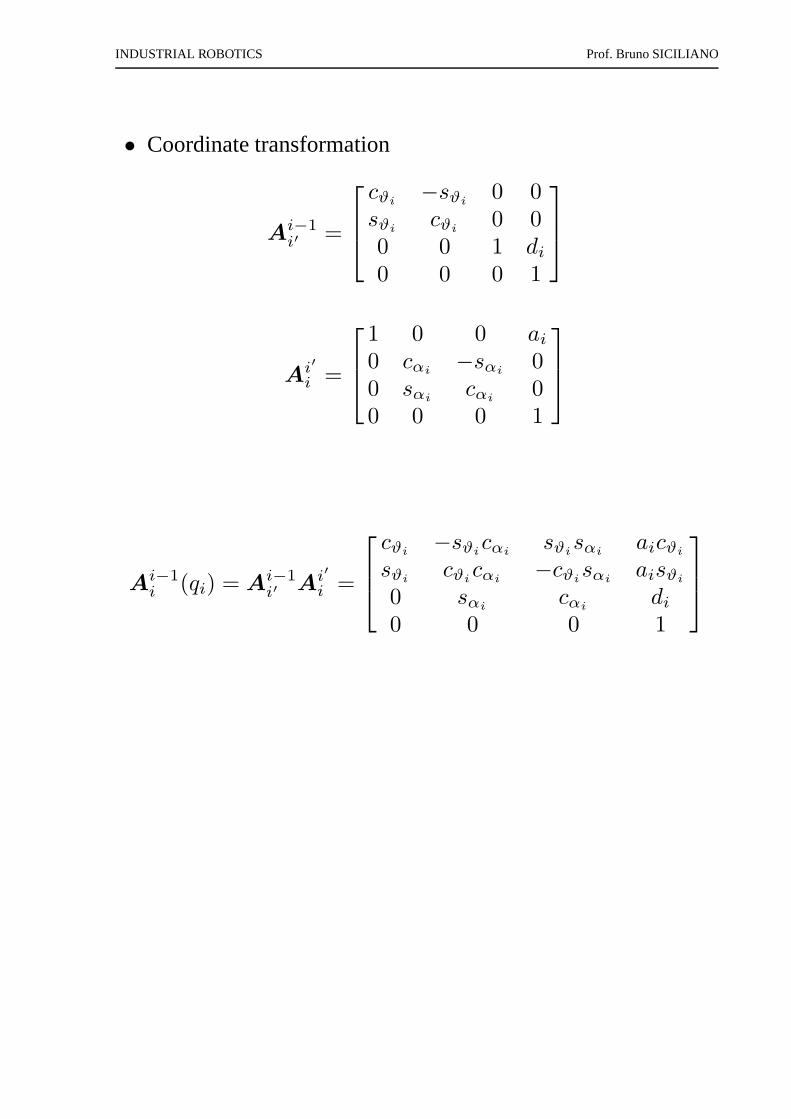
• Coordinate transformation
Ai−1
i′ =
cϑi−sϑi
0 0sϑi
cϑi0 0
0 0 1 di0 0 0 1
Ai′
i =
1 0 0 ai0 cαi
−sαi0
0 sαicαi
00 0 0 1
Ai−1
i (qi) = Ai−1
i′ Ai′
i =
cϑi−sϑi
cαisϑi
sαiaicϑi
sϑicϑicαi
−cϑisαi
aisϑi
0 sαicαi
di0 0 0 1
INDUSTRIAL ROBOTICS Prof. Bruno SICILIANO
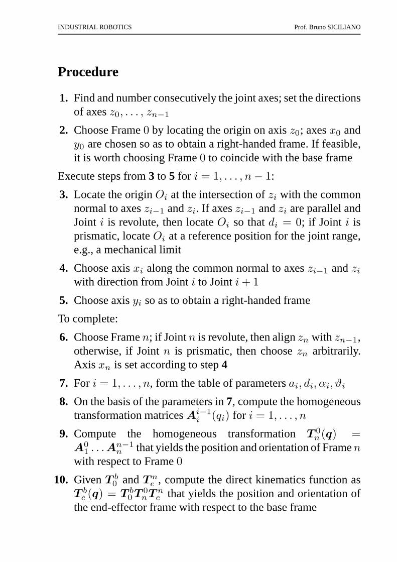
Procedure
1. Find and number consecutively the joint axes; set the directionsof axesz0, . . . , zn−1
2. Choose Frame0 by locating the origin on axisz0; axesx0 andy0 are chosen so as to obtain a right-handed frame. If feasible,it is worth choosing Frame0 to coincide with the base frame
Execute steps from3 to 5 for i = 1, . . . , n− 1:
3. Locate the originOi at the intersection ofzi with the commonnormal to axeszi−1 andzi. If axeszi−1 andzi are parallel andJoint i is revolute, then locateOi so thatdi = 0; if Joint i isprismatic, locateOi at a reference position for the joint range,e.g., a mechanical limit
4. Choose axisxi along the common normal to axeszi−1 andziwith direction from Jointi to Jointi+ 1
5. Choose axisyi so as to obtain a right-handed frame
To complete:
6. Choose Framen; if Jointn is revolute, then alignzn with zn−1,otherwise, if Jointn is prismatic, then choosezn arbitrarily.Axis xn is set according to step4
7. For i = 1, . . . , n, form the table of parametersai, di, αi, ϑi
8. On the basis of the parameters in7, compute the homogeneoustransformation matricesAi−1
i (qi) for i = 1, . . . , n
9. Compute the homogeneous transformationT 0n (q) =
A01 . . .A
n−1n that yields the position and orientation of Framen
with respect to Frame0
10. GivenT b0 andT n
e , compute the direct kinematics function asT be (q) = T b
0 T 0nT n
e that yields the position and orientation ofthe end-effector frame with respect to the base frame
INDUSTRIAL ROBOTICS Prof. Bruno SICILIANO
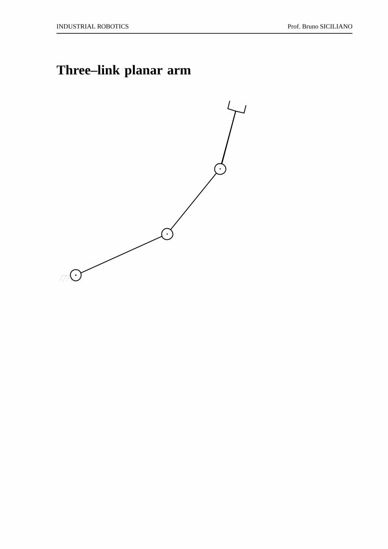
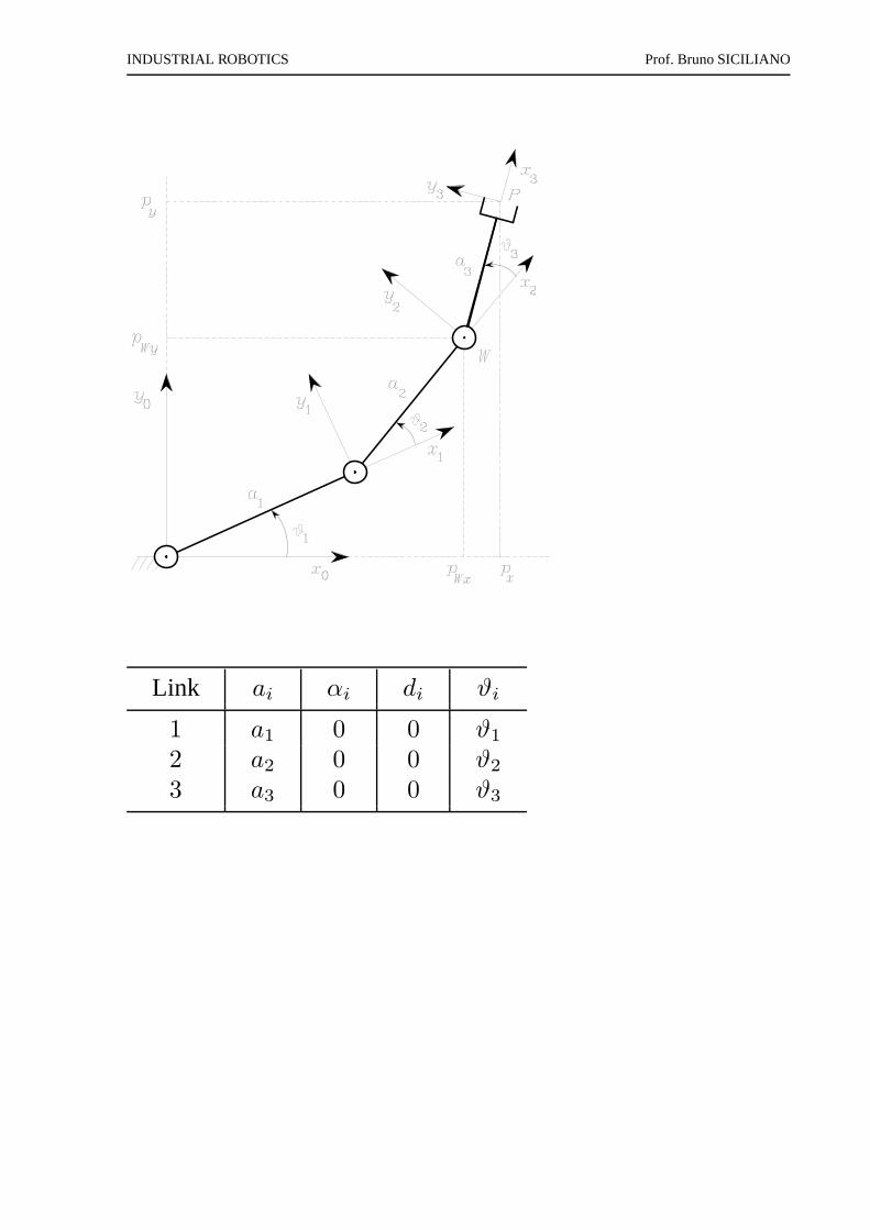
Three–link planar arm
INDUSTRIAL ROBOTICS Prof. Bruno SICILIANO
Link ai αi di ϑi
1 a1 0 0 ϑ1
2 a2 0 0 ϑ2
3 a3 0 0 ϑ3
INDUSTRIAL ROBOTICS Prof. Bruno SICILIANO
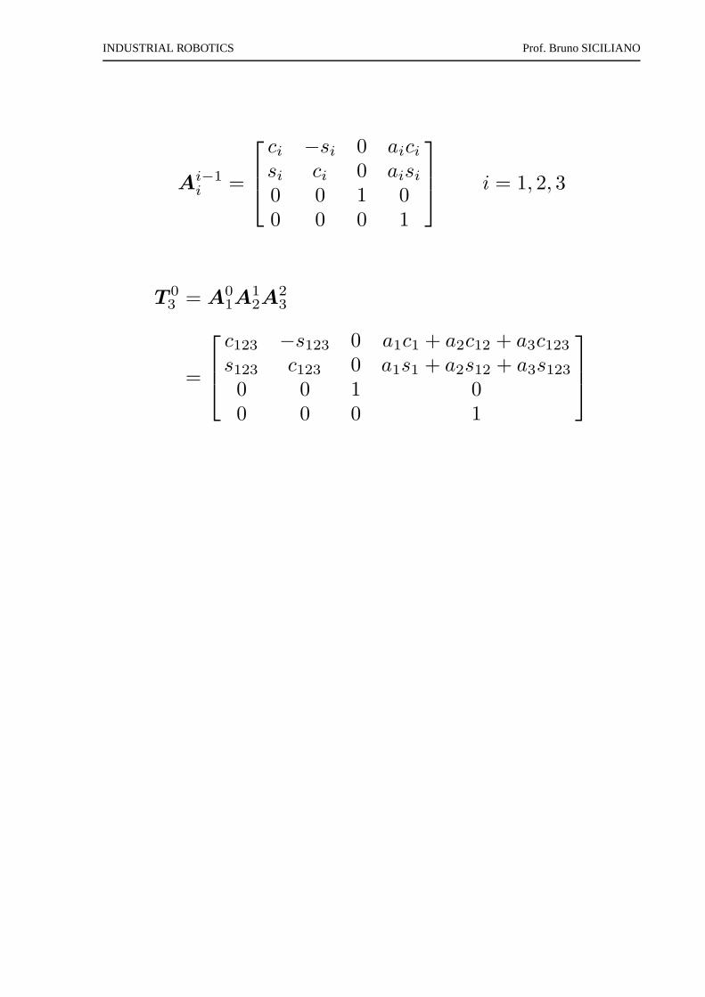
Ai−1
i =
ci −si 0 aicisi ci 0 aisi0 0 1 00 0 0 1
i = 1, 2, 3
T 03 = A0
1A12A
23
=
c123 −s123 0 a1c1 + a2c12 + a3c123s123 c123 0 a1s1 + a2s12 + a3s1230 0 1 00 0 0 1
INDUSTRIAL ROBOTICS Prof. Bruno SICILIANO
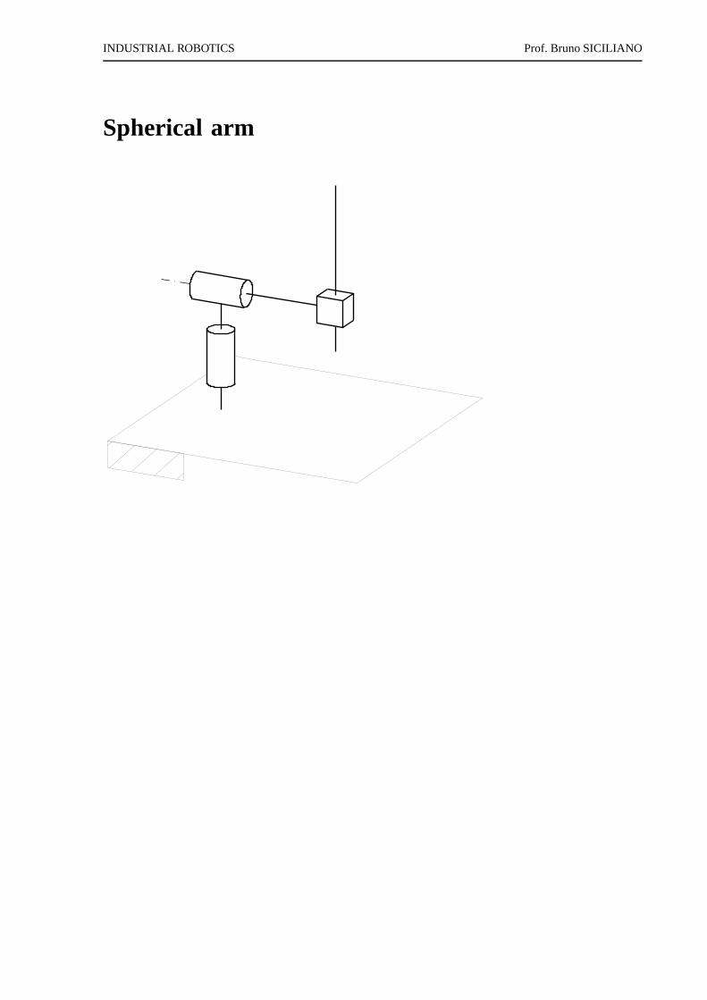
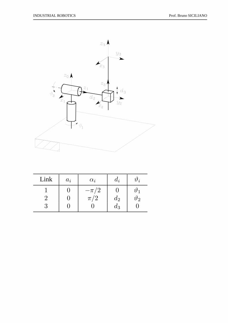
Spherical arm
INDUSTRIAL ROBOTICS Prof. Bruno SICILIANO
Link ai αi di ϑi
1 0 −π/2 0 ϑ1
2 0 π/2 d2 ϑ2
3 0 0 d3 0
INDUSTRIAL ROBOTICS Prof. Bruno SICILIANO
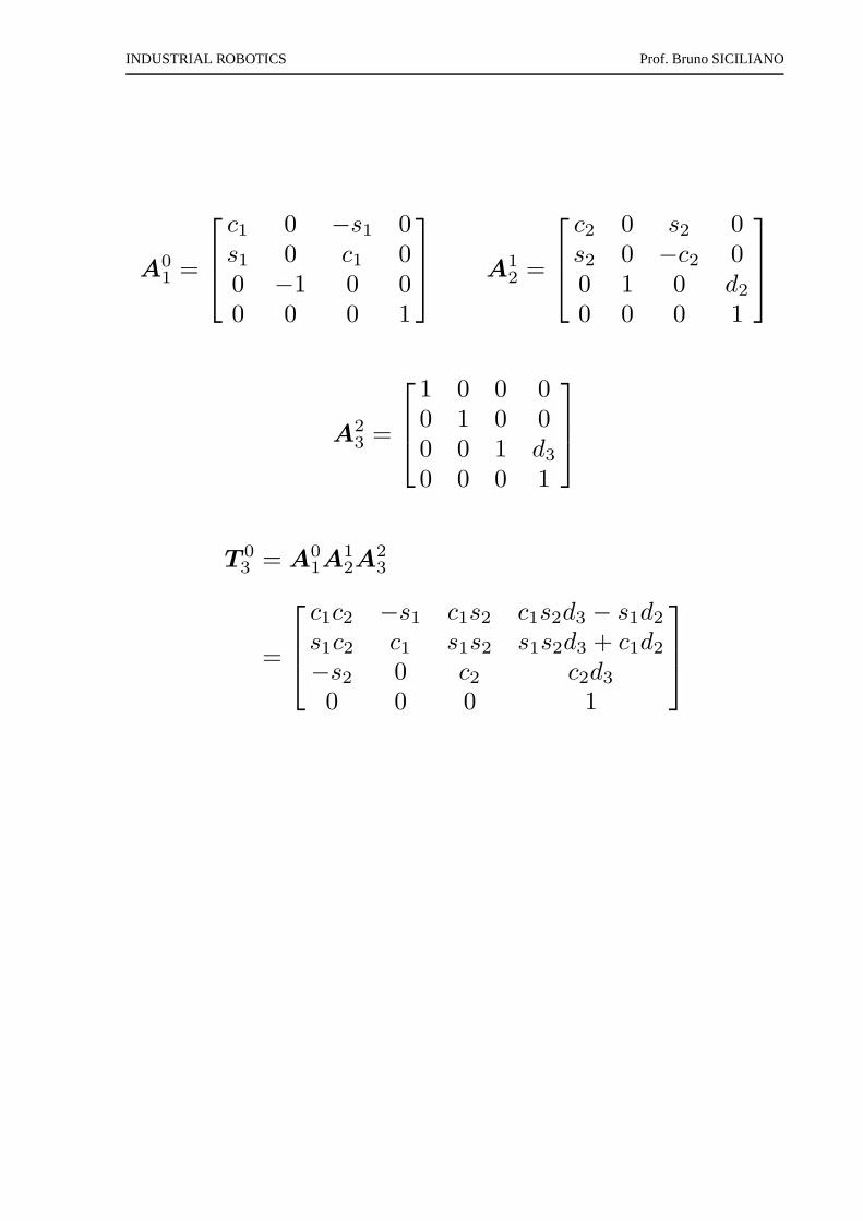
A01 =
c1 0 −s1 0s1 0 c1 00 −1 0 00 0 0 1
A1
2 =
c2 0 s2 0s2 0 −c2 00 1 0 d2
0 0 0 1
A23 =
1 0 0 00 1 0 00 0 1 d3
0 0 0 1
T 03 = A0
1A12A
23
=
c1c2 −s1 c1s2 c1s2d3 − s1d2
s1c2 c1 s1s2 s1s2d3 + c1d2
−s2 0 c2 c2d3
0 0 0 1
INDUSTRIAL ROBOTICS Prof. Bruno SICILIANO
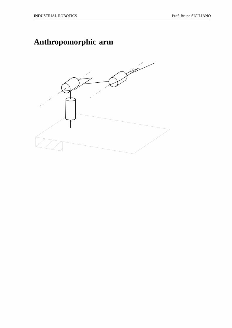
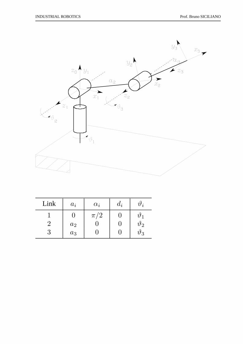
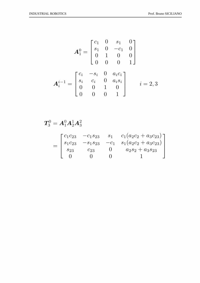
Anthropomorphic arm
INDUSTRIAL ROBOTICS Prof. Bruno SICILIANO
Link ai αi di ϑi
1 0 π/2 0 ϑ1
2 a2 0 0 ϑ2
3 a3 0 0 ϑ3
INDUSTRIAL ROBOTICS Prof. Bruno SICILIANO
A01 =
c1 0 s1 0s1 0 −c1 00 1 0 00 0 0 1
Ai−1
i =
ci −si 0 aicisi ci 0 aisi0 0 1 00 0 0 1
i = 2, 3
T 03 = A0
1A12A
23
=
c1c23 −c1s23 s1 c1(a2c2 + a3c23)s1c23 −s1s23 −c1 s1(a2c2 + a3c23)s23 c23 0 a2s2 + a3s230 0 0 1
INDUSTRIAL ROBOTICS Prof. Bruno SICILIANO
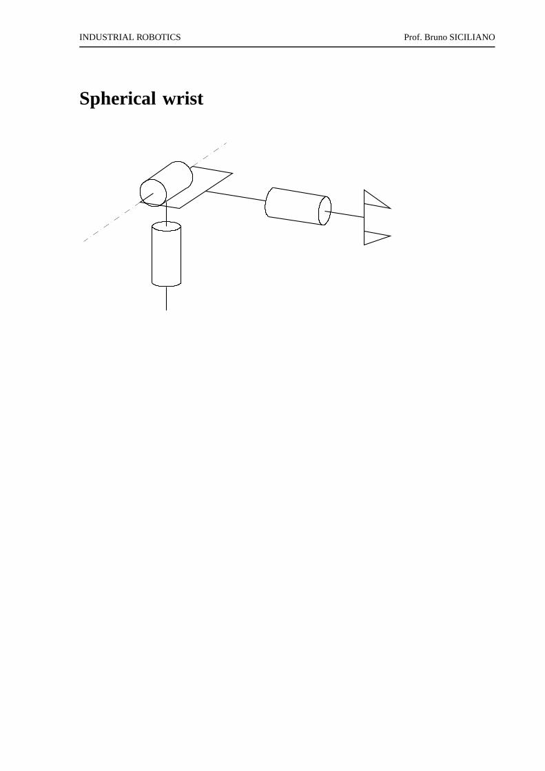
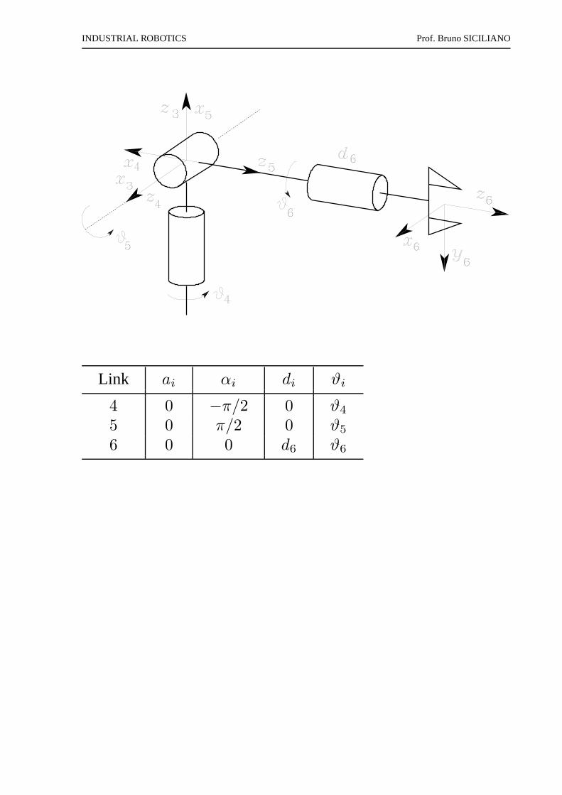
Spherical wrist
INDUSTRIAL ROBOTICS Prof. Bruno SICILIANO
Link ai αi di ϑi
4 0 −π/2 0 ϑ4
5 0 π/2 0 ϑ5
6 0 0 d6 ϑ6
INDUSTRIAL ROBOTICS Prof. Bruno SICILIANO
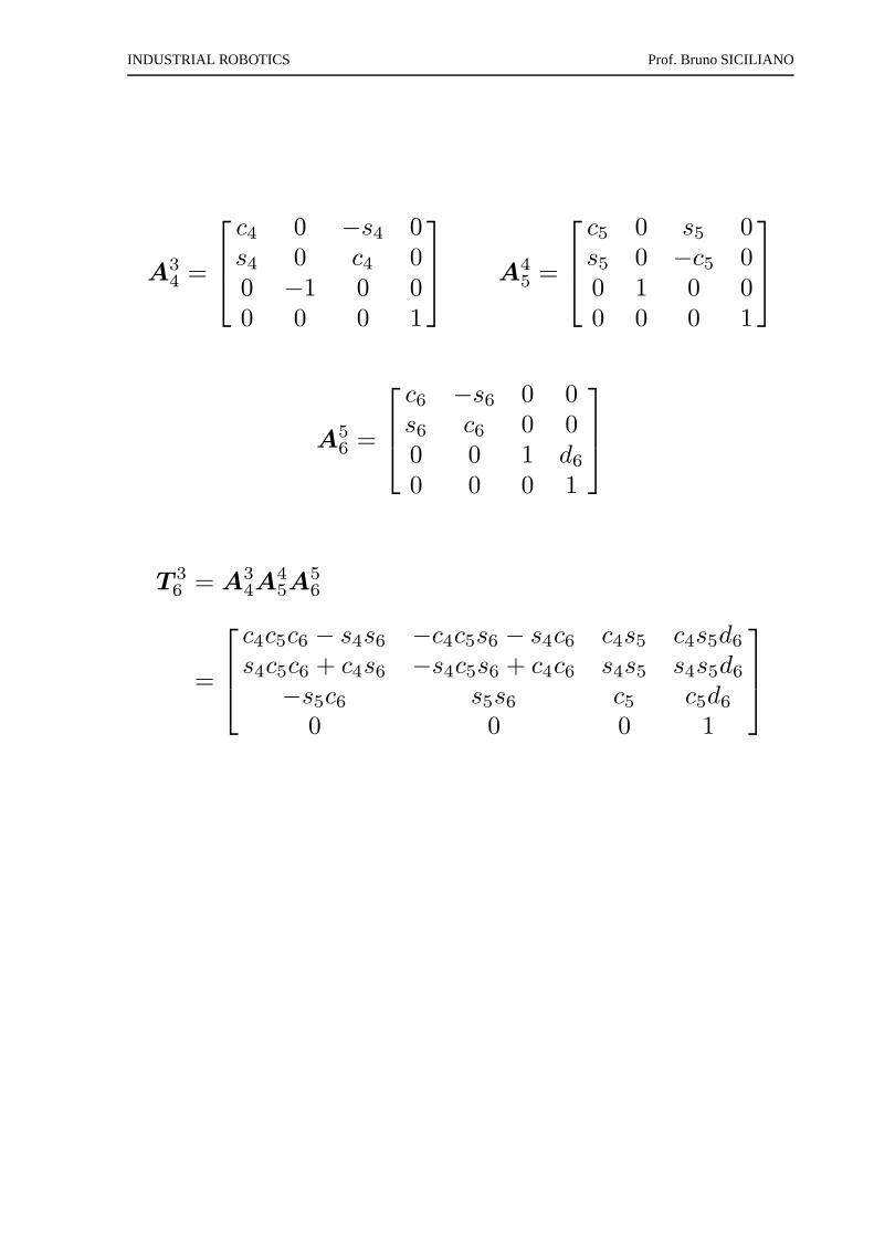
A34 =
c4 0 −s4 0s4 0 c4 00 −1 0 00 0 0 1
A4
5 =
c5 0 s5 0s5 0 −c5 00 1 0 00 0 0 1
A56 =
c6 −s6 0 0s6 c6 0 00 0 1 d6
0 0 0 1
T 36 = A3
4A45A
56
=
c4c5c6 − s4s6 −c4c5s6 − s4c6 c4s5 c4s5d6
s4c5c6 + c4s6 −s4c5s6 + c4c6 s4s5 s4s5d6
−s5c6 s5s6 c5 c5d6
0 0 0 1
INDUSTRIAL ROBOTICS Prof. Bruno SICILIANO
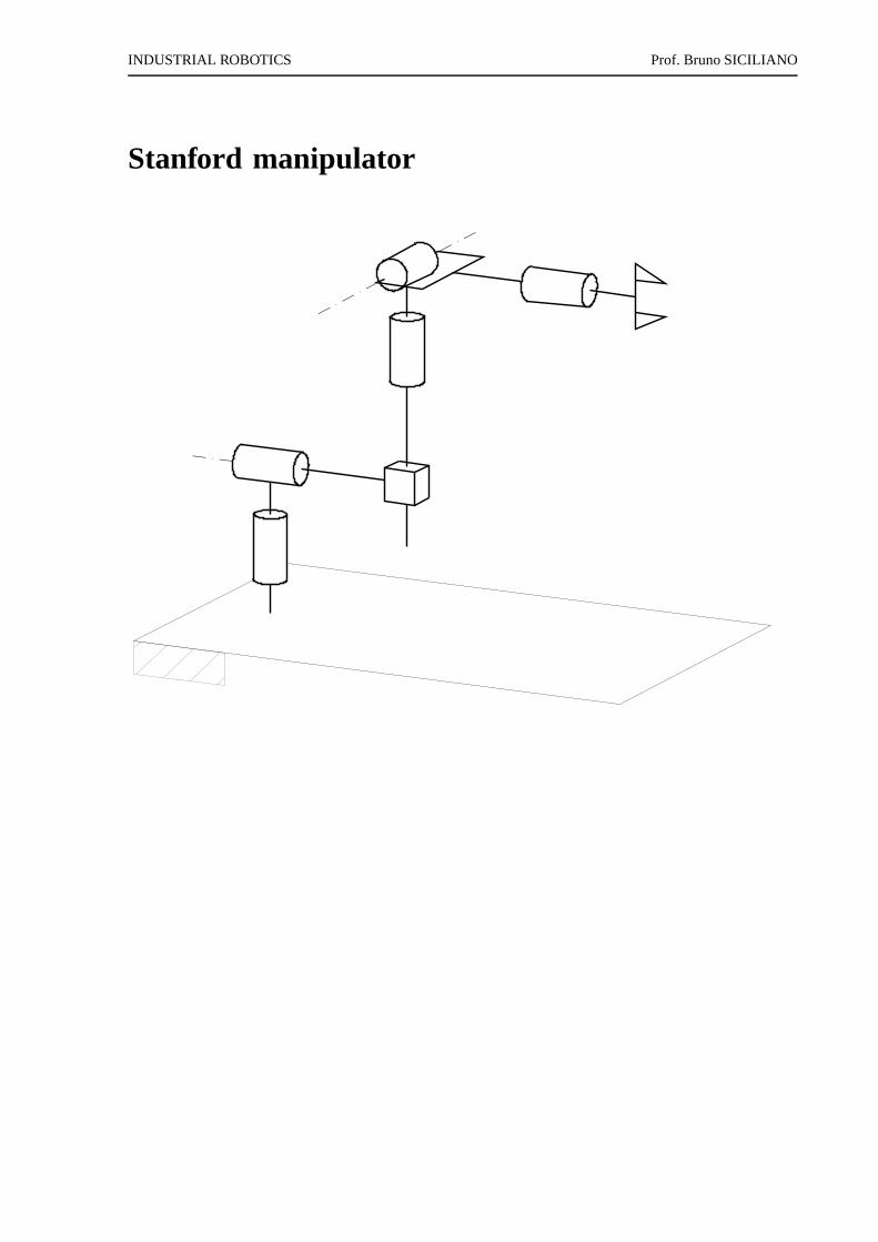
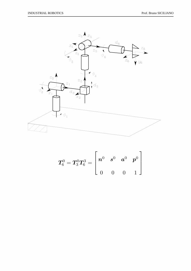
Stanford manipulator
INDUSTRIAL ROBOTICS Prof. Bruno SICILIANO
T 06 = T 0
3 T 36 =
n0 s0 a0 p0
0 0 0 1
INDUSTRIAL ROBOTICS Prof. Bruno SICILIANO
p0 =
c1s2d3 − s1d2 +(
c1(c2c4s5 + s2c5) − s1s4s5)
d6
s1s2d3 + c1d2 +(
s1(c2c4s5 + s2c5) + c1s4s5)
d6
c2d3 + (−s2c4s5 + c2c5)d6
n0 =
c1(
c2(c4c5c6 − s4s6) − s2s5c6)
− s1(s4c5c6 + c4s6)
s1(
c2(c4c5c6 − s4s6) − s2s5c6)
+ c1(s4c5c6 + c4s6)−s2(c4c5c6 − s4s6) − c2s5c6
s0 =
c1(
−c2(c4c5s6 + s4c6) + s2s5s6)
− s1(−s4c5s6 + c4c6)
s1(
−c2(c4c5s6 + s4c6) + s2s5s6)
+ c1(−s4c5s6 + c4c6)s2(c4c5s6 + s4c6) + c2s5s6
a0 =
c1(c2c4s5 + s2c5) − s1s4s5s1(c2c4s5 + s2c5) + c1s4s5
−s2c4s5 + c2c5
INDUSTRIAL ROBOTICS Prof. Bruno SICILIANO
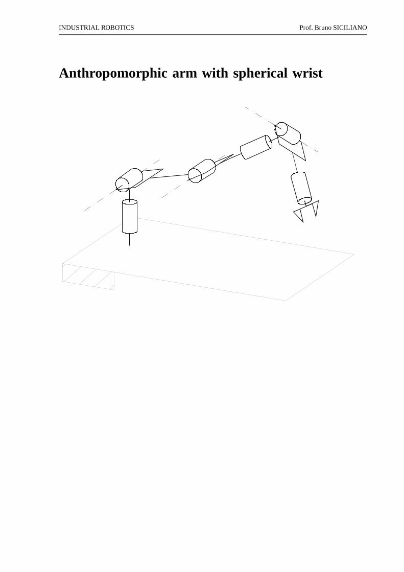
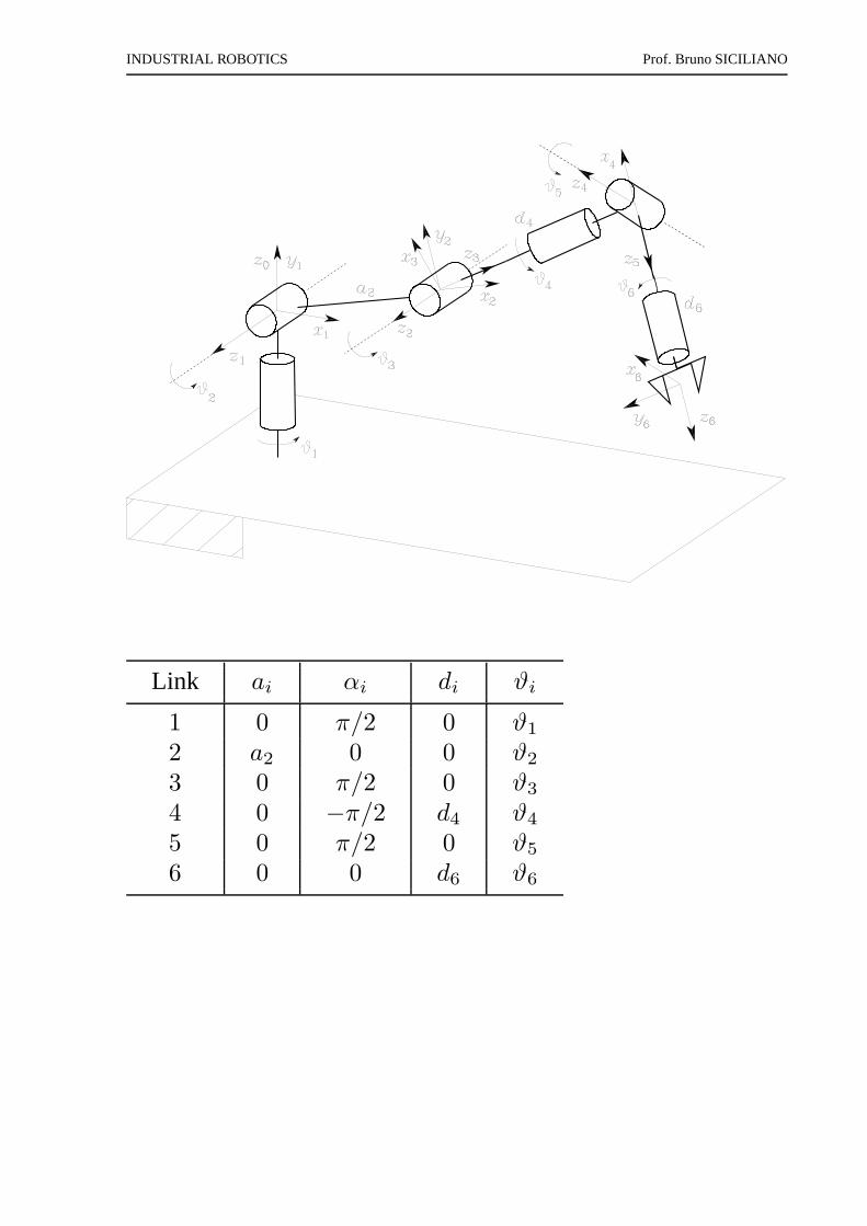
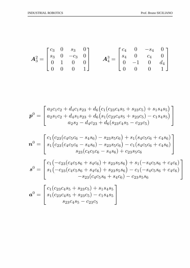
Anthropomorphic arm with spherical wrist
INDUSTRIAL ROBOTICS Prof. Bruno SICILIANO
Link ai αi di ϑi
1 0 π/2 0 ϑ1
2 a2 0 0 ϑ2
3 0 π/2 0 ϑ3
4 0 −π/2 d4 ϑ4
5 0 π/2 0 ϑ5
6 0 0 d6 ϑ6
INDUSTRIAL ROBOTICS Prof. Bruno SICILIANO
A23 =
c3 0 s3 0s3 0 −c3 00 1 0 00 0 0 1
A3
4 =
c4 0 −s4 0s4 0 c4 00 −1 0 d4
0 0 0 1
p0 =
a2c1c2 + d4c1s23 + d6
(
c1(c23c4s5 + s23c5) + s1s4s5)
a2s1c2 + d4s1s23 + d6
(
s1(c23c4s5 + s23c5) − c1s4s5)
a2s2 − d4c23 + d6(s23c4s5 − c23c5)
n0 =
c1(
c23(c4c5c6 − s4s6) − s23s5c6)
+ s1(s4c5c6 + c4s6)
s1(
c23(c4c5c6 − s4s6) − s23s5c6)
− c1(s4c5c6 + c4s6)s23(c4c5c6 − s4s6) + c23s5c6
s0 =
c1(
−c23(c4c5s6 + s4c6) + s23s5s6)
+ s1(−s4c5s6 + c4c6)
s1(
−c23(c4c5s6 + s4c6) + s23s5s6)
− c1(−s4c5s6 + c4c6)−s23(c4c5s6 + s4c6) − c23s5s6
a0 =
c1(c23c4s5 + s23c5) + s1s4s5s1(c23c4s5 + s23c5) − c1s4s5
s23c4s5 − c23c5
INDUSTRIAL ROBOTICS Prof. Bruno SICILIANO
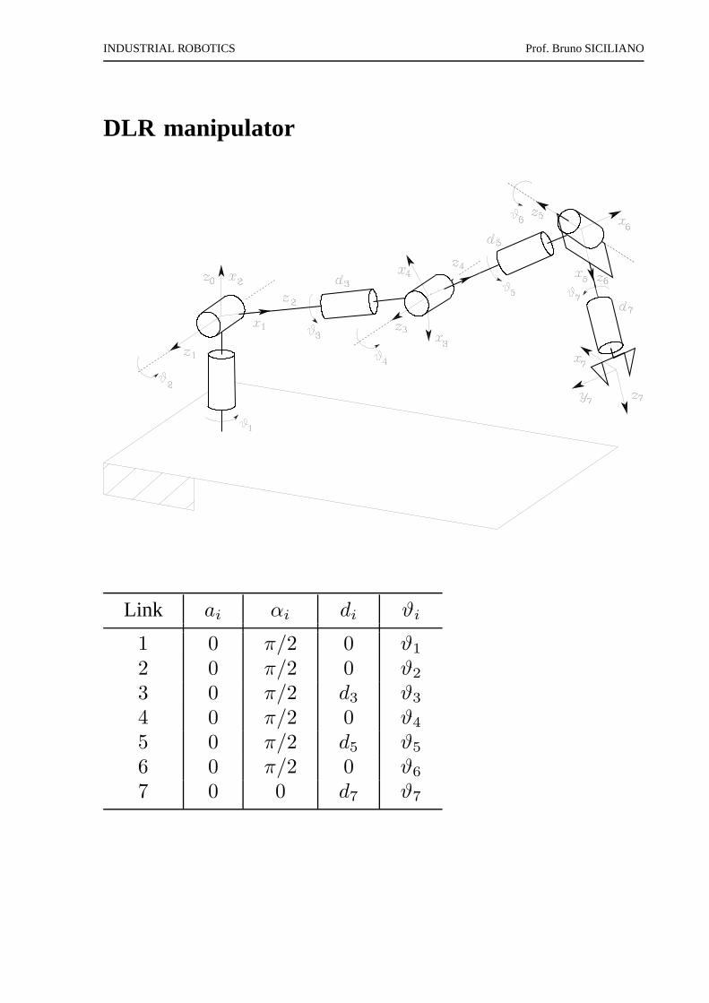
DLR manipulator
Link ai αi di ϑi
1 0 π/2 0 ϑ1
2 0 π/2 0 ϑ2
3 0 π/2 d3 ϑ3
4 0 π/2 0 ϑ4
5 0 π/2 d5 ϑ5
6 0 π/2 0 ϑ6
7 0 0 d7 ϑ7
INDUSTRIAL ROBOTICS Prof. Bruno SICILIANO
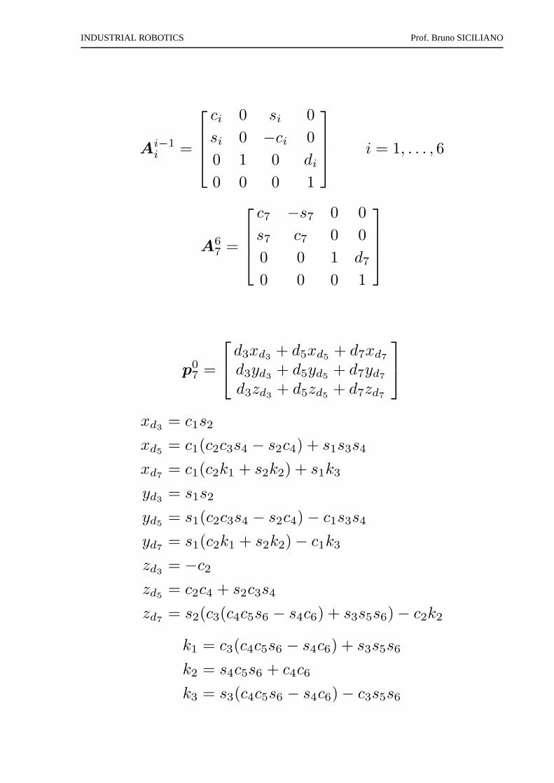
Ai−1
i =
ci 0 si 0
si 0 −ci 0
0 1 0 di
0 0 0 1
i = 1, . . . , 6
A67 =
c7 −s7 0 0
s7 c7 0 0
0 0 1 d7
0 0 0 1
p07 =
d3xd3 + d5xd5 + d7xd7d3yd3 + d5yd5 + d7yd7d3zd3 + d5zd5 + d7zd7
xd3 = c1s2
xd5 = c1(c2c3s4 − s2c4) + s1s3s4
xd7 = c1(c2k1 + s2k2) + s1k3
yd3 = s1s2
yd5 = s1(c2c3s4 − s2c4) − c1s3s4
yd7 = s1(c2k1 + s2k2) − c1k3
zd3 = −c2zd5 = c2c4 + s2c3s4
zd7 = s2(c3(c4c5s6 − s4c6) + s3s5s6) − c2k2
k1 = c3(c4c5s6 − s4c6) + s3s5s6
k2 = s4c5s6 + c4c6
k3 = s3(c4c5s6 − s4c6) − c3s5s6
INDUSTRIAL ROBOTICS Prof. Bruno SICILIANO
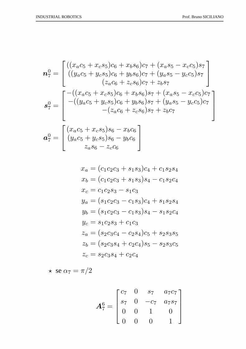
n07 =
((xac5 + xcs5)c6 + xbs6)c7 + (xas5 − xcc5)s7((yac5 + ycs5)c6 + ybs6)c7 + (yas5 − ycc5)s7
(zac6 + zcs6)c7 + zbs7
s07 =
−((xac5 + xcs5)c6 + xbs6)s7 + (xas5 − xcc5)c7−((yac5 + ycs5)c6 + ybs6)s7 + (yas5 − ycc5)c7
−(zac6 + zcs6)s7 + zbc7
a07 =
(xac5 + xcs5)s6 − xbc6(yac5 + ycs5)s6 − ybc6
zas6 − zcc6
xa = (c1c2c3 + s1s3)c4 + c1s2s4
xb = (c1c2c3 + s1s3)s4 − c1s2c4
xc = c1c2s3 − s1c3
ya = (s1c2c3 − c1s3)c4 + s1s2s4
yb = (s1c2c3 − c1s3)s4 − s1s2c4
yc = s1c2s3 + c1c3
za = (s2c3c4 − c2s4)c5 + s2s3s5
zb = (s2c3s4 + c2c4)s5 − s2s3c5
zc = s2c3s4 + c2c4
⋆ seα7 = π/2
A67 =
c7 0 s7 a7c7
s7 0 −c7 a7s7
0 0 1 0
0 0 0 1
INDUSTRIAL ROBOTICS Prof. Bruno SICILIANO
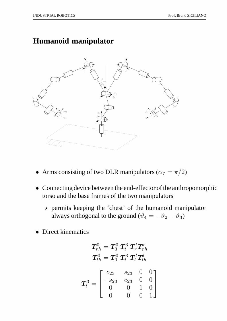
Humanoid manipulator
• Arms consisting of two DLR manipulators (α7 = π/2)
• Connecting device between the end-effector of the anthropomorphictorso and the base frames of the two manipulators
⋆ permits keeping the ‘chest’ of the humanoid manipulatoralways orthogonal to the ground (ϑ4 = −ϑ2 − ϑ3)
• Direct kinematics
T 0rh = T 0
3 T 3t T t
rTrrh
T 0lh = T 0
3 T 3t T t
l Tllh
T 3t =
c23 s23 0 0−s23 c23 0 0
0 0 1 00 0 0 1

INDUSTRIAL ROBOTICS Prof. Bruno SICILIANO
⋆ T 03 like for anthropomorphic manipulator
⋆ T tr andT t
l depend onβ
⋆ T rrh andT l
lh like for DLR manipulator
INDUSTRIAL ROBOTICS Prof. Bruno SICILIANO
JOINT SPACE AND OPERATIONAL SPACE
• Joint space
q =
q1...qn
⋆ qi = ϑi (revolute joint)
⋆ qi = di (prismatic joint)
• Operational space
x =
[
p
φ
]
⋆ p (position)
⋆ φ (orientation)
• Direct kinematics equation
x = k(q)
INDUSTRIAL ROBOTICS Prof. Bruno SICILIANO
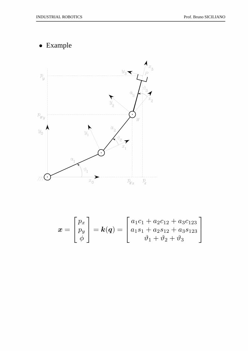
• Example
x =
pxpyφ
= k(q) =
a1c1 + a2c12 + a3c123a1s1 + a2s12 + a3s123
ϑ1 + ϑ2 + ϑ3
INDUSTRIAL ROBOTICS Prof. Bruno SICILIANO
Workspace
• Reachable workspace
p = p(q) qim ≤ qi ≤ qiM i = 1, . . . , n
⋆ surface elements of planar, spherical, toroidal andcylindrical type
• Dexterous workspace
⋆ different orientations
INDUSTRIAL ROBOTICS Prof. Bruno SICILIANO
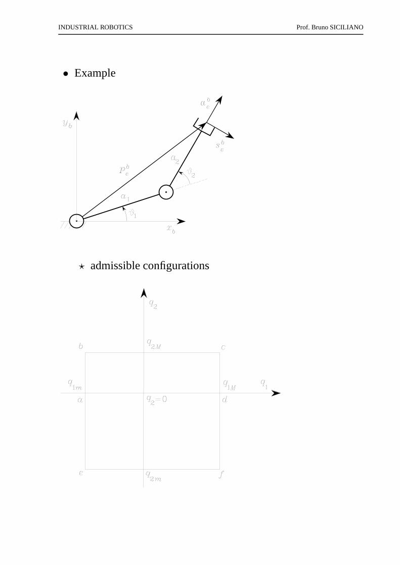
• Example
⋆ admissible configurations
INDUSTRIAL ROBOTICS Prof. Bruno SICILIANO
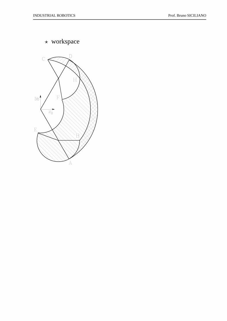
⋆ workspace

INDUSTRIAL ROBOTICS Prof. Bruno SICILIANO
• Accuracy
⋆ deviation between the position reached in the assignedposture and the position computed via direct kinematics
⋆ typical values:(0.2, 1) mm
• Repeatability
⋆ measure of manipulator’s ability to return to a previouslyreached position
⋆ typical values:(0.02, 0.2) mm
• Kinematic redundancy
⋆ m < n (intrinsic)
⋆ r < m = n (functional)
INDUSTRIAL ROBOTICS Prof. Bruno SICILIANO
KINEMATIC CALIBRATION
• Accurate estimates of DH parameters to improve manipulatoraccuracy
• Direct kinematics equation as a function of all parameters
x = k(a,α,d,ϑ)
xm measured pose
xn nominal pose (fixed parameters + joint variables)
∆x =∂k
∂a∆a +
∂k
∂α∆α +
∂k
∂d∆d +
∂k
∂ϑ∆ϑ
= Φ(ζn)∆ζ
INDUSTRIAL ROBOTICS Prof. Bruno SICILIANO
⋆ l measurements (lm≫ 4n)
∆x̄ =
∆x1
...∆xl
=
Φ1
...Φl
∆ζ = Φ̄∆ζ
• Solution
∆ζ = (Φ̄T Φ̄)−1Φ̄T∆x̄
ζ′ = ζn +∆ζ
. . .until ∆ζ converges
⋆ more accurate estimates of fixed parameters
⋆ corrections on transducers measurements
Start-up
• (Home) reference posture
INDUSTRIAL ROBOTICS Prof. Bruno SICILIANO
INVERSE KINEMATICS PROBLEM
• Direct kinematics
⋆ q =⇒ T
⋆ q =⇒ x
• Inverse kinematics
⋆ T =⇒ q
⋆ x =⇒ q
• Complexity
⋆ closed-form solution
⋆ multiple solutions
⋆ infinite solutions
⋆ no admissible solutions
• Intuition
⋆ algebraic
⋆ geometric
• Numerical techniques
INDUSTRIAL ROBOTICS Prof. Bruno SICILIANO
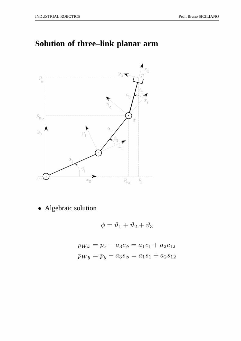
Solution of three–link planar arm
• Algebraic solution
φ = ϑ1 + ϑ2 + ϑ3
pWx = px − a3cφ = a1c1 + a2c12
pWy = py − a3sφ = a1s1 + a2s12
INDUSTRIAL ROBOTICS Prof. Bruno SICILIANO
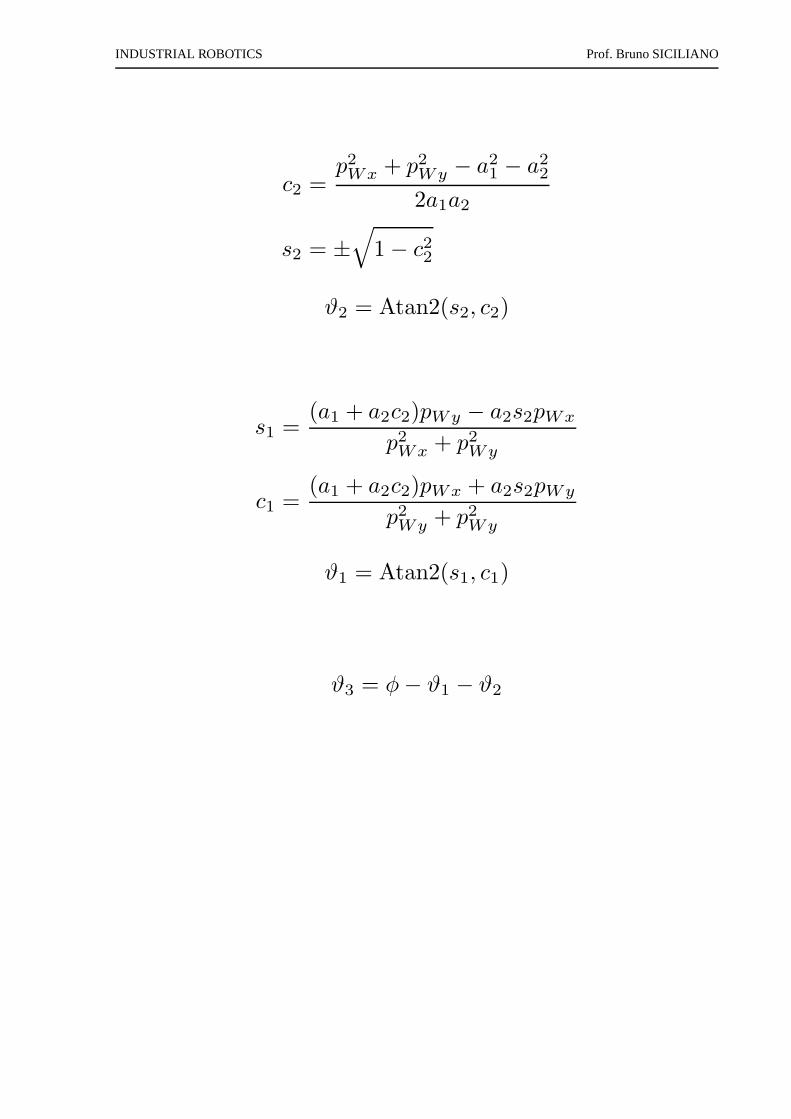
c2 =p2Wx + p2
Wy − a21 − a2
2
2a1a2
s2 = ±√
1 − c22
ϑ2 = Atan2(s2, c2)
s1 =(a1 + a2c2)pWy − a2s2pWx
p2Wx + p2
Wy
c1 =(a1 + a2c2)pWx + a2s2pWy
p2Wy + p2
Wy
ϑ1 = Atan2(s1, c1)
ϑ3 = φ− ϑ1 − ϑ2
INDUSTRIAL ROBOTICS Prof. Bruno SICILIANO
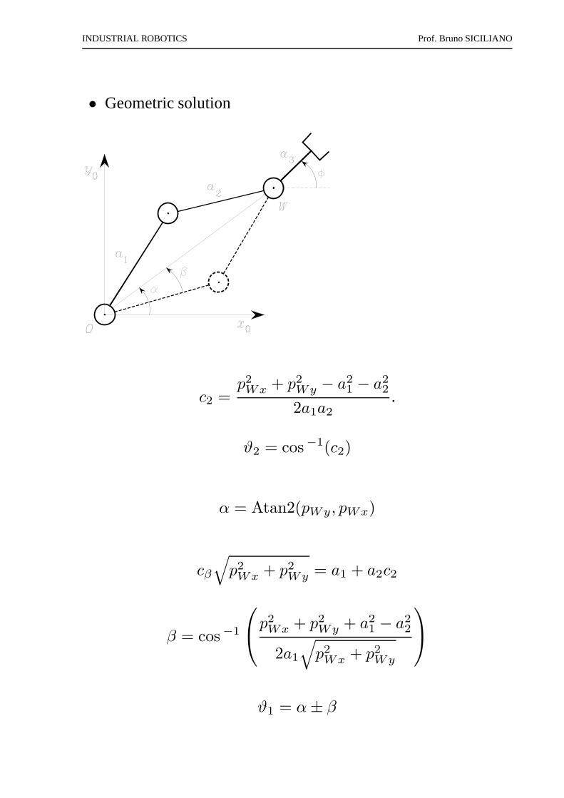
• Geometric solution
c2 =p2Wx + p2
Wy − a21 − a2
2
2a1a2
.
ϑ2 = cos−1(c2)
α = Atan2(pWy, pWx)
cβ
√
p2Wx + p2
Wy = a1 + a2c2
β = cos−1
p2Wx + p2
Wy + a21 − a2
2
2a1
√
p2Wx + p2
Wy
ϑ1 = α± β
INDUSTRIAL ROBOTICS Prof. Bruno SICILIANO
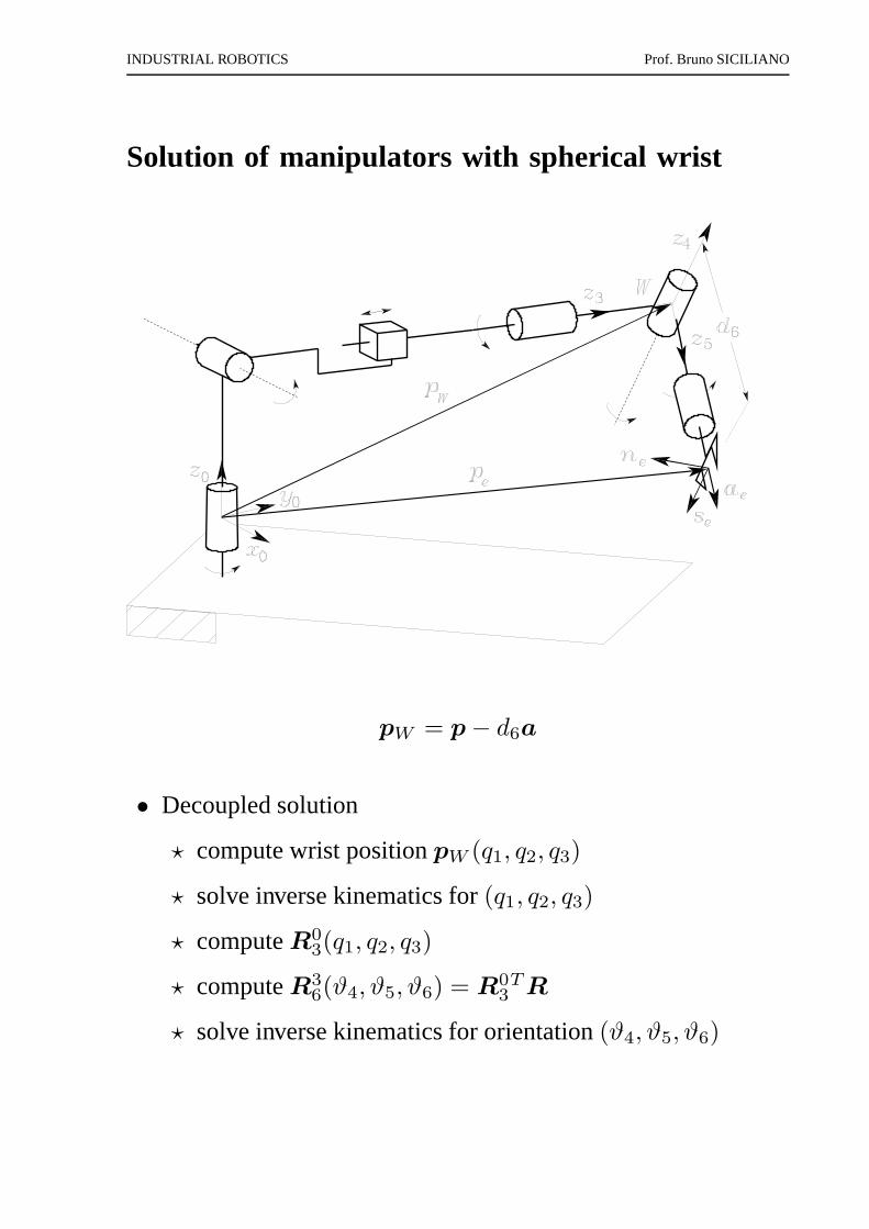
Solution of manipulators with spherical wrist
pW = p − d6a
• Decoupled solution
⋆ compute wrist positionpW (q1, q2, q3)
⋆ solve inverse kinematics for(q1, q2, q3)
⋆ computeR03(q1, q2, q3)
⋆ computeR36(ϑ4, ϑ5, ϑ6) = R0
3TR
⋆ solve inverse kinematics for orientation(ϑ4, ϑ5, ϑ6)
INDUSTRIAL ROBOTICS Prof. Bruno SICILIANO
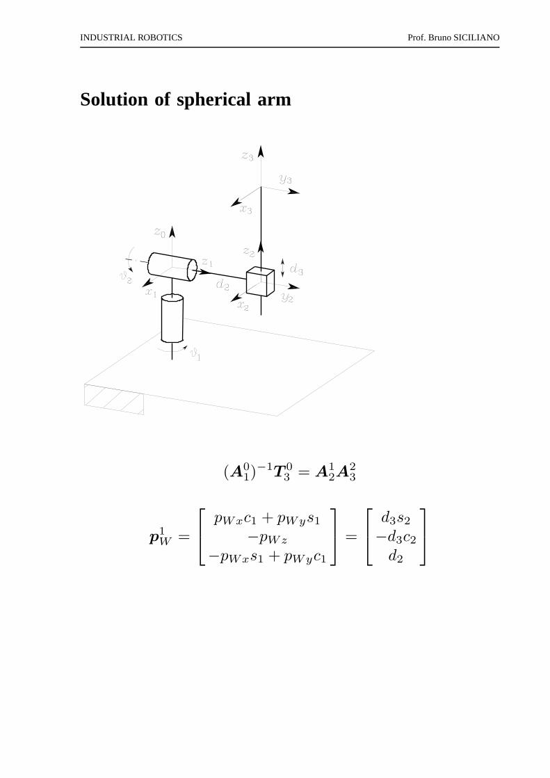
Solution of spherical arm
(A01)
−1T 03 = A1
2A23
p1W =
pWxc1 + pWys1−pWz
−pWxs1 + pWyc1
=
d3s2−d3c2d2
INDUSTRIAL ROBOTICS Prof. Bruno SICILIANO
c1 =1 − t2
1 + t2s1 =
2t
1 + t2
(d2 + pWy)t2 + 2pWxt+ d2 − pWy = 0
ϑ1 = 2Atan2(
−pWx ±√
p2Wx + p2
Wy − d22, d2 + pWy
)
pWxc1 + pWys1−pWz
=d3s2−d3c2
ϑ2 = Atan2(pWxc1 + pWys1, pWz)
d3 =√
(pWxc1 + pWys1)2 + p2Wz

INDUSTRIAL ROBOTICS Prof. Bruno SICILIANO
Solution of anthropomorphic arm
pWx = c1(a2c2 + a3c23)
pWy = s1(a2c2 + a3c23)
pWz = a2s2 + a3s23
c3 =p2Wx + p2
Wy + p2Wz − a2
2 − a23
2a2a3
s3 = ±√
1 − c23
ϑ3 = Atan2(s3, c3)
⇓
INDUSTRIAL ROBOTICS Prof. Bruno SICILIANO
ϑ3,I ∈ [−π, π]
ϑ3,II = −ϑ3,I
INDUSTRIAL ROBOTICS Prof. Bruno SICILIANO
c2 =±
√
p2Wx + p2
Wy(a2 + a3c3) + pWza3s3
a22 + a2
3 + 2a2a3c3
s2 =pWz(a2 + a3c3) ∓
√
p2Wx + p2
Wya3s3
a22 + a2
3 + 2a2a3c3
ϑ2 = Atan2(s2, c2)
⇓
⋆ for s+3 =√
1 − c23:
ϑ2,I = Atan2(
(a2 + a3c3)pWz − a3s+
3
√
p2Wx + p2
Wy,
(a2 + a3c3)√
p2Wx + p2
Wy + a3s+
3 pWz
)
ϑ2,II = Atan2(
(a2 + a3c3)pWz + a3s+
3
√
p2Wx + p2
Wy,
−(a2 + a3c3)√
p2Wx + p2
Wy + a3s+3 pWz
)
⋆ for s−3 = −√
1 − c23:
ϑ2,III = Atan2(
(a2 + a3c3)pWz − a3s−
3
√
p2Wx + p2
Wy,
(a2 + a3c3)√
p2Wx + p2
Wy + a3s−
3 pWz
)
ϑ2,IV = Atan2(
(a2 + a3c3)pWz + a3s−
3
√
p2Wx + p2
Wy,
−(a2 + a3c3)√
p2Wx + p2
Wy + a3s−
3 pWz
)
INDUSTRIAL ROBOTICS Prof. Bruno SICILIANO
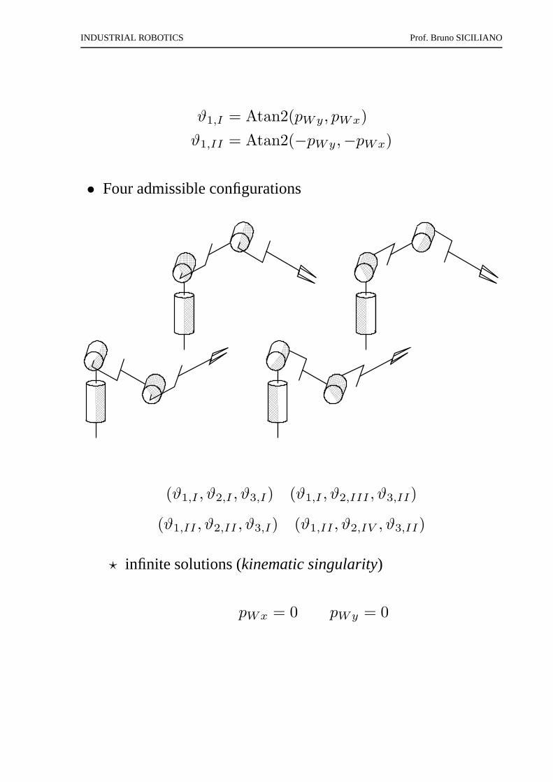
ϑ1,I = Atan2(pWy, pWx)
ϑ1,II = Atan2(−pWy,−pWx)
• Four admissible configurations
(ϑ1,I , ϑ2,I , ϑ3,I) (ϑ1,I , ϑ2,III , ϑ3,II)
(ϑ1,II , ϑ2,II , ϑ3,I) (ϑ1,II , ϑ2,IV , ϑ3,II)
⋆ infinite solutions (kinematic singularity)
pWx = 0 pWy = 0
INDUSTRIAL ROBOTICS Prof. Bruno SICILIANO
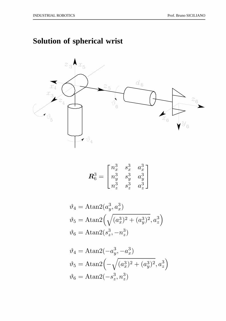
Solution of spherical wrist
R36 =
n3x s3x a3
x
n3y s3y a3
y
n3z s3z a3
z
ϑ4 = Atan2(a3y, a
3x)
ϑ5 = Atan2(√
(a3x)
2 + (a3y)
2, a3z
)
ϑ6 = Atan2(s3z,−n3z)
ϑ4 = Atan2(−a3y,−a3
x)
ϑ5 = Atan2(
−√
(a3x)
2 + (a3y)
2, a3z
)
ϑ6 = Atan2(−s3z, n3z)