rough paths, signatures and the modelling of … paths, signatures and the modelling of functions on...
TRANSCRIPT
Rough paths, Signatures and the modelling
of functions on streams
Terry Lyons∗
Abstract. Rough path theory is focused on capturing and making precise the interac-tions between highly oscillatory and non-linear systems. The techniques draw particularlyon the analysis of LC Young and the geometric algebra of KT Chen. The concepts andtheorems, and the uniform estimates, have found widespread application; the first appli-cations gave simplified proofs of basic questions from the large deviation theory and sub-stantially extending Ito’s theory of SDEs; the recent applications contribute to (Graham)automated recognition of Chinese handwriting and (Hairer) formulation of appropriateSPDEs to model randomly evolving interfaces. At the heart of the mathematics is thechallenge of describing a smooth but potentially highly oscillatory and vector valued pathxt parsimoniously so as to effectively predict the response of a nonlinear system such asdyt = f(yt)dxt, y0 = a. The Signature is a homomorphism from the monoid of paths intothe grouplike elements of a closed tensor algebra. It provides a graduated summary of thepath x. Hambly and Lyons have shown that this non-commutative transform is faithfulfor paths of bounded variation up to appropriate null modifications. Among paths ofbounded variation with given Signature there is always a unique shortest representative.These graduated summaries or features of a path are at the heart of the definition ofa rough path; locally they remove the need to look at the fine structure of the path.Taylor’s theorem explains how any smooth function can, locally, be expressed as a linearcombination of certain special functions (monomials based at that point). Coordinateiterated integrals form a more subtle algebra of features that can describe a stream orpath in an analogous way; they allow a definition of rough path and a natural linear”basis” for functions on streams that can be used for machine learning.
Mathematics Subject Classification (2010). Primary 00A05; Secondary 00B10.
Keywords. Rough paths, Regularity Structures, Machine Learning, Functional Regres-
sion, Numerical Approximation of Parabolic PDE, Shuffle Product, Tensor Algebra
∗Acknowledges the support of the Oxford-Man Institute, the support provided by ERC ad-vanced grant ESig (agreement no. 291244), and particularly the contributions of his colleaguesand his students without whom none of this would have happened and in addition to Kelly Wy-att, Justin Sharp, Ni Hao and Danyu Yang for helping the author finalise this mss. The dataanalysis is is reproduced from the cited paper with Gyurko et al., Gyurko did the analysis, ManGroup provided the initial data for that paper.

2 Terry Lyons
Contents
1 A path or a text? 3
2 Financial Data or a Semimartingale 4
3 Paths - Simply Everywhere - Evolving systems 4
4 A simple model for an interacting system 5
5 Remarkable Estimates (for p > 1) 8
6 The Log Signature 10
7 The ODE method 11
8 Going to Rough Paths 12
9 Coordinate Iterated Integrals 13
10 Expected Signature 14
11 Computing Expected Signatures 15
12 Characteristic Functions of Signatures 16
13 Moments are complicated 16
14 Regression onto a feature set 17
15 The obvious feature set for streams 18
16 Machine learning, an amateur’s first attempt 19
17 Linear regression onto a law on paths 23

Learning from Signatures 3
1. A path or a text?
The mathematical concept of a path embraces the notion of an evolving or timeordered sequence of events, parameterised by a continuous variable. Our mathe-matical study of these objects does not encourage us to think broadly about thetruly enormous range of ”paths” that occur. This talk will take an analyst’s per-spective, we do not expect to study a particular path but rather to find broad brushtools that allow us to study a wide variety of paths - ranging form very ”pure”mathematical objects that capture holonomy to very concrete paths that describefinancial data. Our goal will be to explain the progress we have made in the last50 years or so in describing such paths effectively, and some of the consequencesof these developments.
Let us start by noting that although most mathematicians would agree ona definition of a path, most have a rather stereotyped and limited imaginationabout the variety of paths that are ”in the wild”. One key observation is thatin most cases we are interested in paths because they represent some evolutionthat interacts with and influences some wider system. Another is that in mostpaths, in standard presentations, the content and influence are locked into complexmultidimensional oscillations.
The path in the figure is a piece of text. Each character is coded as a byte andeach byte is represented as four steps with each in one of four directions. It caneasily be represented in other ways, for example as a sequence of printed letters,perhaps in different fonts or bit resolutions. Each represents a stream which hasbroadly the same effect on a coarse scale although the detailed texture is perhapsa bit different.

4 Terry Lyons
2. Financial Data or a Semimartingale
One important source of sequential data comes from financial markets. An intrinsicfeature of financial markets is that they are high dimensional but there is a strongnotion of sequencing of events. Buying with future knowledge is forbidden. Muchof the information relates to prices, and one of the radical successes of appliedmathematics over the last 20-30 years came out of the approximation of priceprocesses by simple stochastic differential equations and semimartingales and theuse of Ito’s calculus. However, modern markets are not represented by simpleprice processes. Most orders happen on exchanges, where there are numerousbids, offers, and less commonly, trades. Much activity in markets is concernedwith market making and the provision of liquidity; decisions to post to the marketare based closely on expectation of patterns of behaviour, and most decisions aresomewhat distant from any view about fundamental value. If one is interested inalerting the trader who has a bug in his code, or understanding how to trade a largeorder without excessive charges then the semi-martingale model has a misplacedfocus. The data in the figure is actual activity on a market for oil futures over a
79.5
79.52
79.54
79.56
79.58
79.6
79.62
79.64
79.66
1
12
23
34
45
56
67
78
89
10
0
11
1
12
2
13
3
14
4
15
5
16
6
17
7
18
8
19
9
21
0
22
1
23
2
24
3
25
4
26
5
27
6
28
7
29
8
30
9
32
0
33
1
34
2
35
3
36
4
37
5
38
6
39
7
40
8
41
9
43
0
44
1
45
2
46
3
47
4
48
5
49
6
Pri
ce
Tick
500 Ticks
Bid
Ask
Last Traded Price
Source: QuantHouse, 2012 (www. quanthouse.com)
Oil Futures
15 minute period. One can see a lot of structure but a semi-martingale model forprices captures little of it.
3. Paths - Simply Everywhere - Evolving systems
Informally, a stream is a map γ from a totally ordered set I to some state space,where we are interested in the effect (or transformation of state) this streamachieves. As we have noted the same stream of information can admit differ-ent representations with different fidelity. When the totally ordered set I is an

Learning from Signatures 5
interval and there are reasonable path properties (e.g. such as right continuity)we will call the stream a path. Nonetheless, many interesting streams are finiteand discrete. There are canonical and informative ways to convert them [10] tocontinuous paths.
It is worth noting that, even at this abstract level, there are natural mathe-matical operations and invariances that are applied to a stream. One can repa-rameterise the speed at which one examines the stream and simultaneously thespeed at which one looks at the effects. One can split a stream into two or moresegments (a coproduct). One can sub-sample a stream. In general we will focuson those streams which are presented in a way where such sub-sampling degradesthe information in the stream gradually. One can also merge or interleave discretestreams according to their time stamps if the totally ordered sets I, I ′can be in-terleaved. All of these properties are inherited for the properties of totally orderedsets. If the target ”effect” or state space is linear there is also the opportunityto translate and so concatenate streams or paths [15] and so get richer algebraicstructures. One of the most interesting and economically important questions onecan ask about a stream is how to summarise (throw away irrelevant information)so as to succinctly capture its effects:
text schoolchild precissound audio engineer faithful perception
web page search provider interest for readerweb click history advertiser effective ad placementbrownian path numerical analysis effective simulation
rough paths analyst RDEsWhat is actually quite surprising is that there is a certain amount of useful workone can do on this problem that does not depend on the nature of the stream orpath.
4. A simple model for an interacting system
We now focus on a very specific framework where the streams are maps from a realinterval, that we will intuitively refer to as the time domain, into an a Banach spacethat we will refer to as the state space. We will work with continuous paths incontinuous time but, as we mentioned, there are canonical ways to embed discretetick style data into this framework using the Hoff process and in financial contextsthis is important. There is also a more general theory dealing with paths withjumps [Williams, Simon].
6 Terry Lyons
4.1. Controlled Differential Equations. A path is a map γ from aninterval J = [J−, J+] into a Banach space E. The dimension of E may well befinite, but we allow for the possibility that it is not. It has bounded (p-)variationif
sup...ui<ui+1...∈[J−,J+]
∑i
∥∥γui+1− γu
∥∥ < ∞
sup...ui<ui+1...∈[J−,J+]
∑i
∥∥γui+1− γu
∥∥p < ∞
where p ≥ 1 In our context the path γ is controlling the system, and we are inter-ested in its effect as measured by y and the interactions between γ and y. It wouldbe possible to use the theory of rough paths to deal with the internal interactions ofautonomous and ”rough” systems, one specific example of deterministic McKeanVlasov type is [4].
Separately there needs to be a space F that carries the state of the system anda family of different ways to evolve. We represent the dynamics on F through thespace Ω (F ) of vector fields on F. Each vector field provides a different way for thestate to evolve. We connect this potential to evolve the state in F to the controlγ via a linear map
V : Elinear→ Ω (F ) .
Immediately we can see the controlled differential equation
dyt = V (yt) dγt, yJ− = a
πJ(yJ−)
: = yJ+
provides a precise framework allowing for the system y to respond to γ accordingto the dynamics V . We call such a system a controlled differential equation.
The model of a controlled differential equation is a good one. Many differenttypes of object can be positioned to fit the definition. Apart from the more obviousapplied examples, one can view a finite automata (in computer science sense) andthe geometric concept of lifting a path along a connection as producing examples.
Lemma 4.1 (Reparameterisation). If τ : I → J is an increasing homeomorphism,and if
dyt = V (yt) dγt, yJ− = a,
then the reparameterised control produces the reparameterised effect:
dyτ(t) = V(yτ(t)
)dγτ(t), yτ(I−) = a.
Lemma 4.2 (Splitting). Let πJ be the diffeomorphism capturing the transfor-mational effect of γ|J . Let t ∈ J . Then πJ can be recovered by composing thediffeomorpisms π[J−,t], π[t,J+] associated with splitting the interval J at t and con-sidering the composing the effect of γ|
[J−,t]and γ|[t,J+] separately:
π[t,J+]π[J−,t] = πJ .
Learning from Signatures 7
In this way we see that, assuming the vector fields were smooth enough tosolve the differential equations uniquely and for all time, a controlled differentialequation is a homomorphism from the monoid of paths with concatenation intothe diffeomorphisms/transformations of the state space. By letting π act as anoperator on functions we see that every choice of V defines a representation of themonoid of paths in E
Remark 4.3 (Subsampling). Although there is a good behaviour with respectto sub-sampling, which in effect captures and quantifies the numerical analysis ofthese equations, it is more subtle and we do not make it explicit here.
Remark 4.4. Fixing V , restricting γ to smooth paths on [0, 1] and consideringthe solutions y with y0 = a, generically the closure of the set of pairs (γ, y) in theuniform topology is NOT the graph of a map; γ → y is not closable and so is notwell defined as a (even an unbounded and discontinuous) function in the space ofcontinuous paths. Different approximations lead to different views as to what thesolution should be.
4.2. Linear Controlled Differential Equations. Where the controlγ is fixed and smooth, the state space is linear, and all the vector fields are linear,then the space of responses y, as one varies the starting location a, is a linearspace and π[S,T ] : a = yS → yT is a linear automorphism. This case is essentiallyCartan’s development of a path in a aeaLie Algebra into a path in the aeaLieGroup starting at the identity. From our point of view it is a very important specialcase of our controlled differential equations; it reveals one of the key objects wewant to discuss in this paper.
Suppose F is a Banach space, and A is a linear map E → HomR (F, F ) andthat γt is a path in E. Consider the linear differential equation
dyt = Aytdγt.
By iterating using Picard iteration one obtains
yJ+=
∞∑n=0
An∫· · ·∫
J−≤u1≤...≤un≤J+
dγu1⊗ . . .⊗ dγun
y0
The Signature of γ over the interval J = [J−, J+]
Definition 4.5. The Signature S of a path γ over the interval J = [J−, J+] is thetensor sequence
S (γ|J) :=
∞∑n=0
∫· · ·∫
u1≤...≤un∈Jn
dγu1⊗ . . .⊗ dγun
∈∞⊕n=0
E⊗n
It is sometimes written S (γ)J or S (γ)J−,J+.
8 Terry Lyons
Lemma 4.6. The path t→ S (γ)0,t solves a linear differential equation controlledby γ.
Proof. The equation is the universal non-commutative exponential:
dS0,t = S0,t ⊗ dγt.S0,0 = 1
The solution to any linear equation is easily expressed in terms of the Signature
dyt = Aytdγt
yJ+
=
( ∞∑0
AnSnJ
)yJ−
(1)
πJ =
∞∑0
AnSnJ
and we will see in the next sections that this series converges very well and eventhe first few terms in S are effective in describing the response yT leading to theview that γ|J → S (γ|J) is a transform with some value. The use of S to describesolutions to linear controlled differential equations goes back at least to Chen, andFeynman. The magic is that one can estimate the errors in convergence of theseries (1) without detailed understanding of γ or A.
5. Remarkable Estimates (for p > 1)
It seems strange, and even counter intuitive, that one should be able to identifyand abstract a finite sequence of features or coefficients describing γ adequately sothat its effect on a broad range of different systems could be accurately predictedwithout detailed knowledge of the system A or the path - beyond those few co-efficients. But that is the truth of it, there are easy uniform estimates capturingthe convergence of the series (1) based entirely on the length (or more generallyp-rough path variation) of the control and the norm of A as a map from E to thelinear vector fields on F .
Lemma 5.1. If γ is a path of finite variation on J with length |γJ | <∞, then
SnJ : =
∫· · ·∫
u1≤...≤un∈Jn
dγu1⊗ . . .⊗ dγun
≤ |γJ |n
n!

Learning from Signatures 9
giving uniform error control∥∥∥∥∥∥∥yJ+ −N−1∑
0
An∫· · ·∫
J−≤u1≤...≤un≤J+
dγu1 ⊗ . . .⊗ dγuny0
∥∥∥∥∥∥∥ ≤( ∞∑n=N
‖A‖n |γJ |n
n!
)‖y0‖ .
Proof. Because the Signature of the path always solves the characteristic differen-tial equation it follows that one can reparameterise the path γ without changingthe Signature of γ. Reparameterise γ so that it is defined on an interval J oflength |γ| and runs at unit speed. Now there are n!disjoint simplexes inside a cubeobtained by different permuted rankings of the coordinates and thus
‖SnJ ‖ : =
∥∥∥∥∥∥∫· · ·∫
u1≤...≤un∈Jn
dγu1 ⊗ . . .⊗ dγun
∥∥∥∥∥∥=
∥∥∥∥∥∥∫· · ·∫
u1≤...≤un∈Jn
γu1⊗ . . .⊗ γun
du1 . . . dun
∥∥∥∥∥∥=
∫· · ·∫
u1≤...≤un∈Jn
‖γu1⊗ . . .⊗ γun
‖ du1 . . . dun
=
∫· · ·∫
u1≤...≤un∈Jn
du1 . . . dun
=|γJ |n
n!.
from which the second estimate is clear.
The Poisson approximation of a normal one learns at high school ensures thatthe estimates on the right become very sharply estimated in terms of λ→∞ andpretty effective as soon as N ≥ ‖A‖ |γJ |+ λ
√‖A‖ |γJ |.
Remark 5.2. The uniform convergence of the series
N−1∑n=0
An∫· · ·∫
J−≤u1≤...≤un≤J+
dγu1⊗ . . .⊗ dγun
y0
and the obvious continuity of the terms of the series in the inputs (A, γ, y0) guar-antees that the response yT is jointly continuous (uniform limits of continuousfunctions are continuous) in (A, γ, y0) where γ is given the topology of 1-variation(or any of the rough path metrics). It is already the case that
γ →∫· · ·∫
J−≤u1≤u2≤J+
dγu1⊗ dγu2
fails the closed graph property in the uniform metric.
10 Terry Lyons
6. The Log Signature
It is easy to see that the Signature of a path segment actually takes its values ina very special curved subspace of the tensor algebra. Indeed, Chen noted that themap S is a homomorphism of path segments with concatenation into the algebra,and reversing the path segment produces the inverse tensor. As a result one seesthat the range of the map is closed under multiplication and has inverses so it is agroup (inside the grouplike elements) in the tensor series. It is helpful to think ofthe range of this Signature map as a curved space in the tensor series. As a resultthere is a lot of valuable structure. One important map is the logarithm; it is oneto one on the group and provides a flat parameterisation of the group in terms ofelements of the free aeaLie series.
Definition 6.1. If γt ∈ E is a path segment and S is its Signature then
S = 1 + S1 + S2 + . . . ∀i, Si ∈ E⊗i
log (1 + x) = x− x2/2 + . . .
logS =(S1 + S2 + . . .
)−(S1 + S2 + . . .
)2/2 + . . .
The series logS =(S1 + S2 + . . .
)−(S1 + S2 + . . .
)2/2+ . . . which is well defined,
is referred to as the log Signature of γ.
Because the space of tensor series T ((E)) :=⊕∞
0 E⊗n is a unital associativealgebra under ⊗,+ it is also a aeaLie algebra, and with [A,B] := A⊗B −B ⊗A.
Definition 6.2. There are several canonical aeaLie algebras associated to T ((E)) ;weuse the notation L (E) for the algebra generated by E (the space of aeaLie poly-nomials), L(n) (E) the projection of this into T (n) (E) = T ((E)) /
⊕∞n+1E
⊗m (theaeaLie algebra of the free nilpotent group Gn of n steps) and L ((E)) the projectivelimit of the L(n) (E) (the aeaLie Series).
Because we are working in characteristic zero, we may take the exponential,and this recovers the Signature, so no information is lost. A key observationof Chen [6]was that if γ is a path segment then logS (γ) ∈ L ((E)). The mapfrom paths [23, 8]to L(n) (E) via the projection πn : T ((E)) → T (n) (E) is onto.Up to equivalence under a generalised notion of reparameterisation of paths, themap from paths γ of finite length in E to their Signatures S (γ) ∈ T ((E)) orlog-Signatures logS ∈ L ((E)) is injective [?].However the range of this map inL ((E)) ,although well behaved under integer multiplication is not closed underinteger division [21] and so the aeaLie algebra of the group of tree reduced pathsis well defined but not a linear space; it is altogether a more subtle object.
Implicit in the definition of a controlled differential equation
dyt = f (yt) dγt, y0 = a
is the map f . This object takes an element e ∈ E and an element y ∈ F andproduces a second vector in F.representing the infinitesimal change to the state

Learning from Signatures 11
y of the system that will occur if γ is changed infinitesimally in the direction e.This author is clear that the best way to think about f is as a linear map from thespace E into the vector fields on F . In this way one can see that the integral off along γ in its simplest form is a path in the aeaLie algebra and that in solvingthe differential equation we are developing that path into the group. Now, at leastformally, the vector fields are a aeaLie algebra (for the diffemorphisms of F) andsubject to the smoothness assumptions we can take aeaLie brackets to get newvector fields. Because L ((E)) is the free aeaLie algebra over E Chapter II, [2]anylinear map f of E into a aeaLie algebra g induces a unique aeaLie map extensionf∗ to a aeaLie map from L ((E)) to g. This map can be readily implemented andis well defined because of the abstract theory
e → f (e) a vector field
e1e2 − e2e1 → f (e1) f (e2)− f (e2) f (e1) a vector field
f : L(n) (E)→ vector fields.
although in practice one does not take the map to the full projective limit.
7. The ODE method
The linkage between truncations of the log-Signature in L ((E)) and vector fieldson Y is a practical one for modelling and understanding controlled differentialequations. It goes well beyond theory and underpins some of the most effectiveand stable numerical approaches (and control mechanisms) for translating the in-formation in the control γ into information about the response.
If dyt = f (yt) dγt, and yJ− = a then how can we use the first few terms ofthe (log-)Signature of γ to provide a good approximation to yJ+? We could usepicard iteration, or better an euler method based on a Taylor series in terms ofthe Signatures. Picard iteration for exp z already illustrates one issue. Picardinteration yields a power series as approximation - fine if z = 100,but awful ifx = −100. However, there is a more subtle problem to do with stability thatalmost all methods based on Taylor series have - stability - they can easily produceapproximations that are not feasible. These are aggravated in the controlled casebecause of the time varying nature of the systems. It can easily happen that thesolutions to the vector fields are hamiltonian etc. The ODE method uses the firstfew terms of the Signature to construct a time invariant ODE (vector field) that ifone solves it for unit time, it provides an approximation to the desired solution. Itpushes the numerics back onto state of the art ODE solvers. Providing the ODEsolver is accurate and stable then the approximation to y will also be. One can usesymplectic solvers etc. At the level of rough paths, the approximation is obtainedby replacing the path γ with a new rough path γ (a geodesic in the nilpotent groupGn) with the same first few terms in the Signature; this guarantees the feasibilityof the approximations. Today, rough path theory can be used to estimate thedifference between the solution and the approximation in terms of the distancebetween γ and γ even in infinite dimensions.[5][3]
12 Terry Lyons
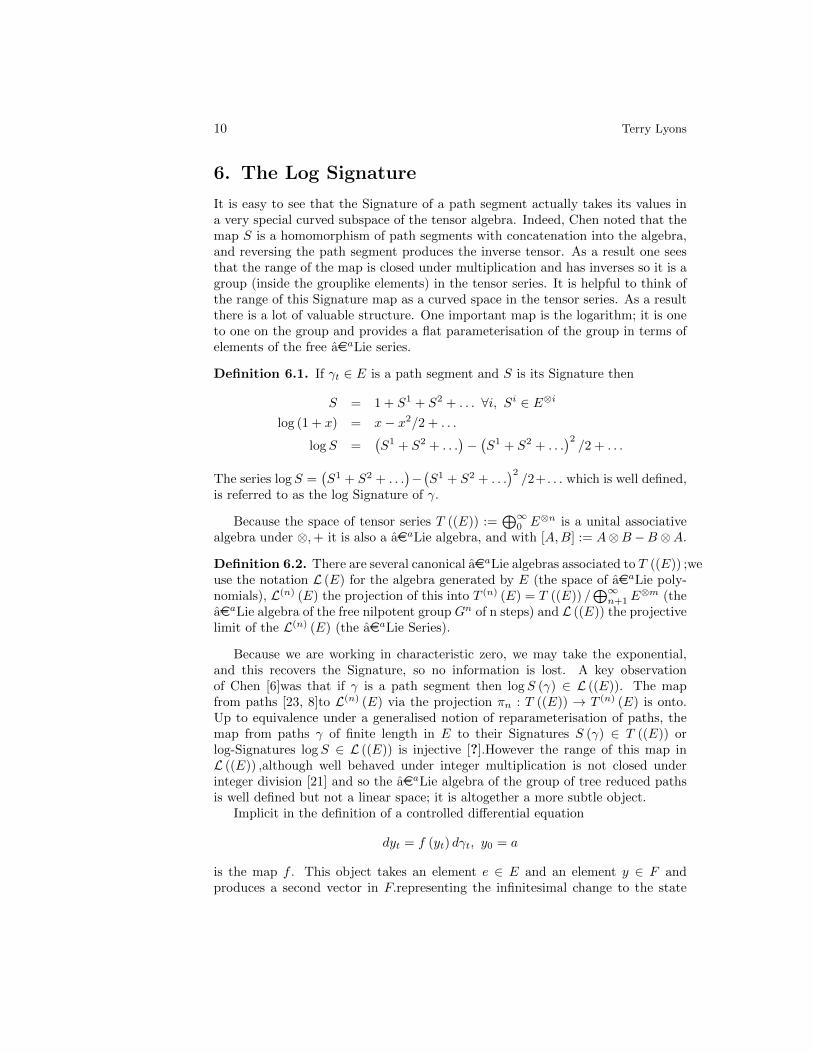
Remark 7.1. A practical numerical scheme can be built as follows.
1. Describe γ over a short interval J in terms of first few terms of logS(γ[J−,J+]
)expressed as a linear combination of terms of a fixed hall basis:
logSJ = l1 + l2 + . . . ∈ L ((E))
l(n) = πn (logSJ) = l1 + . . .+ ln ∈ L(n) (E)
l1 =∑i
λiei
l2 =∑i<j
λij [ei, ej ] ,
. . .
and use this information to produce a path dependent vector field V =f(l(n)).
2. Use an appropriate ODE solver to solve the ODE xt = V (xt), where x0 =yJ− . A stable high order approximation to yJ+
is given by xJ+.
3. Repeat over small enough time steps for the high order approximations tobe effective.
4. The method is high order, stable, and corresponding to replacing γ with apiecewise geodesic path on successively finer scales.
8. Going to Rough Paths
As this is a survey, we have deliberately let the words rough path enter the textbefore they are introduced more formally. Rough path theory answers the followingquestion. Suppose that γ is a smooth path but still on normal scales, a highly roughand oscillatory path. Suppose that we have some smooth system f . Give a simplemetric on paths γ and a continuity estimate that ensures that if two paths thatare close in this metric then their responses are quantifiably close as well. Theestimate should only depend on f through its smoothness. There is such a theory[20], and a family of rough path metrics which make the function γ → y uniformlycontinuous. The completion of the smooth paths γ under these metrics are therough paths we speak about. The theory extends to an infinite dimensional oneand the estimates are uniform in a way that does not depend on dimension.
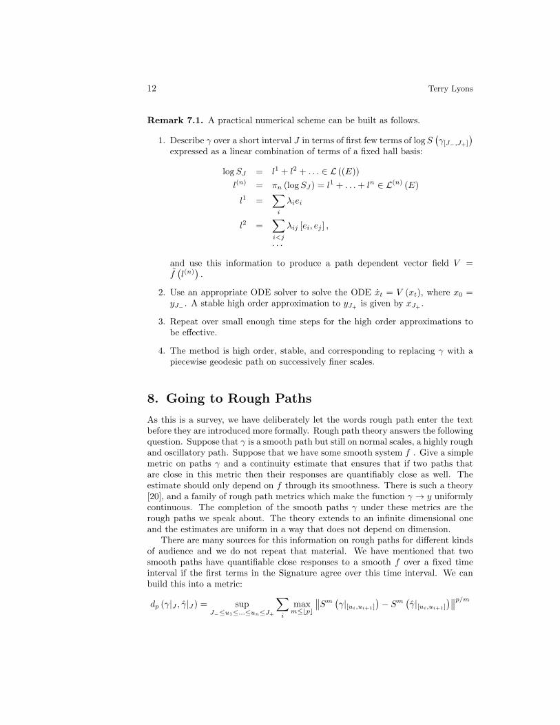
There are many sources for this information on rough paths for different kindsof audience and we do not repeat that material. We have mentioned that twosmooth paths have quantifiable close responses to a smooth f over a fixed timeinterval if the first terms in the Signature agree over this time interval. We canbuild this into a metric:
dp (γ|J , γ|J) = supJ−≤u1≤...≤un≤J+
∑i
maxm≤bpc
∥∥Sm (γ|[ui,ui+1]
)− Sm
(γ|[ui,ui+1]
)∥∥p/m
Learning from Signatures 13
and providing the system is Lip (p+ ε) the response will behave uniformly with thecontrol. The completion of the piecewise smooth paths under dp are p-variationpaths. They do not have smoothness but they do have a ”top down” descriptionand can be viewed as living in a bpc-step nilpotent group over E.
There is a big difference between the Kolmogorov view, xti ∈ Oi, and therough path view - in the latter it is not enough to know where a path is at timet. Instead for small intervals [ui, ui+1], one describes the increment of the pathover the interval. More accurately one describes the approximate effect of the pathsegment into a simple nonlinear system (the lift onto a nilpotent group). Knowingthis information in an analytically adequate way is all one needs to know to predictits effect on a general system.
The whole rough path theory is very substantial and we cannot survey it ad-equately here. The range is wide, and is related to any situation where one hasa family of non-commuting operators and one wants to do analysis on apparentlydivergent products and for example it is interesting to understand the paths onegets as partial integrals of complex Fourier transform as the nonlinear Fouriertransform is a differential equation driven by this path. Some results have beenobtained in this direction [22] while the generalisations to spatial contexts are sohuge that they are spoken about elsewhere at this congress. Many books are nowwritten on the subject [11].and new lecture notes by Friz are to appear soon withrecent developments. So in what is left of this paper we will focus on one topic theSignature of a path and the expected Signature of the path with a view to par-tially explaining how it is really an extension of Taylor’s theorem to various infinitedimensional groups, and how we can get practical traction from this perspective.One key point we will not mention is that using Taylor’s theorem twice works!This is actually a key point that the whole rough path story depends on and whichvalidates its use. One needs to read the proofs to understand this adequately and,except for this sentence, suppress it completely here.
9. Coordinate Iterated Integrals
In this short paper we have to have a focus, and as a result we cannot explorethe analysis and algebra needed to fully describe rough paths or to discuss thespatial generalisations directly even though they are having great impact[14][13].Nonetheless much of what we say can be though of as useful foundations for thiswork. We are going to focus on the Signature as a tool for understanding pathsand as a new tool to help with machine learning.
The essential remark may seem a bit daunting to an analyst, but will be stan-dard to others. The dual of the enveloping algebra of a group(like) object has anatural abelian product structure and linearises polynomial functions on a group.This fact allows one to use linear techniques on the linear spaces to approximategeneric smooth (and nonlinear) functions on the group. Here the group is the”group” of paths.
Monomials are special functions on Rn, and polynomials are linear combina-
14 Terry Lyons
tions of these monomials. Because monomials span an algebra, the polynomialsare able to approximate any continuous function on a compact set. Coordinateiterated integrals are linear functionals on the tensor algebra and at the same timethey are the monomials or the features on path space.
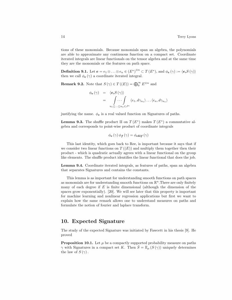
Definition 9.1. Let e = e1⊗ . . .⊗ en ∈ (E∗)⊗n ⊂ T (E∗), and φe (γ) := 〈e,S (γ)〉
then we call φe (γ) a coordinate iterated integral.
Remark 9.2. Note that S (γ) ∈ T ((E)) =⊕∞
0 E⊗n and
φe (γ) = 〈e,S (γ)〉
=
∫· · ·∫
u1≤...≤un∈Jn
〈e1, dγu1〉 . . . 〈en, dγun
〉
justifying the name. φe is a real valued function on Signatures of paths.
Lemma 9.3. The shuffle product q on T (E∗) makes T (E∗) a commutative al-gebra and corresponds to point-wise product of coordinate integrals
φe (γ)φf (γ) = φeqf (γ)
This last identity, which goes back to Ree, is important because it says that ifwe consider two linear functions on T ((E)) and multiply them together then theirproduct - which is quadratic actually agrees with a linear functional on the grouplike elements. The shuffle product identifies the linear functional that does the job.
Lemma 9.4. Coordinate iterated integrals, as features of paths, span an algebrathat separates Signatures and contains the constants.
This lemma is as important for understanding smooth functions on path spacesas monomials are for understanding smooth functions on Rn.There are only finitelymany of each degree if E is finite dimensional (although the dimension of thespaces grow exponentially). [20]. We will see later that this property is importantfor machine learning and nonlinear regression applications but first we want toexplain how the same remark allows one to understand measures on paths andformulate the notion of fourier and laplace transform.
10. Expected Signature
The study of the expected Signature was initiated by Fawcett in his thesis [9]. Heproved
Proposition 10.1. Let µ be a compactly supported probability measure on pathsγ with Signatures in a compact set K. Then S = Eµ (S (γ)) uniquely determinesthe law of S (γ) .

Learning from Signatures 15
Proof. Consider Eµ(φe (γ)).
Eµ(φe (γ)) = Eµ (〈e,S (γ)〉)= 〈e,Eµ (S (γ))〉
=⟨e,S⟩
Since the e with the shuffle product form an algebra and separate points of K theStone-Weierstrass Theorem implies they form a dense subspace in C (K) and sodetermine the law of the Signature of γ.
Given this lemma it immediately becomes interesting to ask how does onecompute Eµ (S). Also, Eµ (S) is like a Laplace transform and will fail to exist forreasons of tail behaviour of the random variables. Is there a characteristic function?Can we identify the general case where the expected Signature determines the lawin the non-compact case. All of these are fascinating and important questions.Partial answers and strong applications are emerging. One of the earliest was therealisation that one could approximate effectively to a complex measure such asWiener measure by a measure on finitely many paths that has the same expectedSignature on T (n) (E)[19, 17].
11. Computing Expected Signatures
Computing Laplace and Fourier transforms can often be a challenging problemfor undergraduates. In this case suppose that X a Brownian motion with Levyarea on a bounded C1 domain Ω ⊂ Rd,stopped on first exit. The following resultexplains how one may construct the expected Signature as a recurrence relation inPDEs[18].
Theorem 11.1. Let
F (z) : = Ez(S(X|[0,TΩ]
))F ∈ S
((Rd))
F = (f0, f1, . . . , )
Then F satisfies and is determined by a PDE finite difference operator
∆fn+2 = −d∑i=1
ei ⊗ ei ⊗ fn − 2
d∑i=1
ei ⊗∂
∂zifn+1
f0 ≡ 1, f1 ≡ 0, and fj |∂Ω ≡ 0, j > 0
Combining this result with Sobolev and regularity estimates from PDE theoryallow one to extract much nontrivial information about the underlying measurealthough it is still open whether in this case the expected Signature determines
16 Terry Lyons
the measure. This question is difficult even for brownian motion on min(Tτ , t)although (unpublished) it looks as if the question can be resolved.
Other interesting questions about expected Signatures can be found for examplein [1].
12. Characteristic Functions of Signatures
It is possible to build a characteristic function out of the expected Signature bylooking at the linear differential equations corresponding to development of thepaths into finite dimensional unitary groups. These linear images of the Signatureare always bounded and so expectations always make sense.
Consider SU (d) ⊂M (d) and realise su (d) as the space of traceless Hermitianmatrices and consider
ψ : E → su (d)
dΨt = ψ (Ψt) dγt.
Theorem 12.1. Ψt is a linear functional on the tensor algebra restricted to theSignatures S
(γ|[0,t]
)and is given by a convergent series. It is bounded and so its ex-
pectation as γ varies randomly always makes sense. The function ψ → E(ΨJ+
(S))
is an extended characteristic function.
Proposition 12.2. ψ → Ψ (S) (polynomial identities of Gambruni and Valentini)span an algebra and separate Signatures as ψ and d vary.
Corollary 12.3. The laws of measures on Signatures are completely determinedby ψ → E (Ψ (S))
Proof. Introduce a polish topology on the grouplike elements.
These results can be found in [7], the paper also gives a sufficient conditionfor the expected Signature to determine the law of the underlying measure onSignatures.
13. Moments are complicated
The question of determining the Signature from its moments seems quite hard atthe moment.
Example 13.1. Observe that if X is N (0, 1) then although X3 is not determinedby its moments, if Y = X3 then (X,Y ) is. The moment information implies
E((Y −X3
)2)= 0.
We repeat our previous question. Does the expected Signature determine thelaw of the Signature for say stopped brownian motion. The problem seems tocapture the challenge.
Learning from Signatures 17
Lemma 13.2 ([7]). If the radius of convergence of∑znE ‖Sn‖ is infinite then the
expected Signature determines the law.
Lemma 13.3 ([18]). If X a Brownian motion with Levy area on a bounded C1
domain Ω ⊂ Rd then∑znE ‖Sn‖ has at the least a strictly positive lower bound
on the radius of curvature.
The gap in understanding between the previous two results is, for the author,a fascinating and surprising one that should be closed!
14. Regression onto a feature set
Learning how to regress or learn a function from examples is a basic problem inmany different contexts. In what remains of this paper, we will outline recent workthat explains how the Signature engages very naturally with this problem and whyit is this engagement that makes it valuable in rough path theory too.
We should emphasise that the discussion and examples we give here is at a veryprimitive level of fitting curves. We are not trying to do statistics, or model andmake inference about uncertainty. Rather we are trying to solve the most basicproblems about extracting relationships from data that would exist even if onehad perfect knowledge. We will demonstrate that this approach can be easy toimplement and effective in reducing dimension and doing effective regression. Wewould expect Baysian statistics to be an added layer added to the process whereuncertanty exists in the data that can be modelled reasonably.
A core idea in many successful attempts to learn functions from a collectionof known (point, value) pairs revolves around the identification of basic func-tions or features that are readily evaluated at each point and then try to expressthe observed function a linear combination of these basic functions. For exam-ple one might evaluate a smooth function ρ at a generic collection xi ∈ [0, 1]of points producing pairs (yi = ρ (xi) , xi) Now consider as feature functionsφn : x→ xn, n = 0, . . . N. These are certainly easy to compute for each xi.Wetry to express
ρ 'N∑n=0
λnφn
and we see that if we can do this (that is to say ρ is well approximated by apolynomial) then the λn are given by the linear equation
yj =
N∑n=0
λnφn (xj) .
In general one should expect, and it is even desirable, that the equations aresignificantly degenerate. The purpose of learning is presumably to be able to usethe function
∑Nn=0 λnφn to predict ρ on new and unseen values of x and to at least
be able to replicate the observed values of y.
18 Terry Lyons
There are powerful numerical techniques for identifying robust solutions tothese equations. Most are based around least squares and singular value decom-position, along with L1 constraints and Lasso.
However, this approach fundamentally depends on the assumption that theφn span the class of functions that are interesting. It works well for monomialsbecause they span an algebra and so every Cn (K) function can be approximatedin Cn (K) by a multivariate real polynomial. It relies on a priori knowledge ofsmoothness or Lasso style techniques to address over-fitting.
I hope the reader can now see the significance of the coordinate iterated inte-grals. If we are interested in functions (such as controlled differential equations)that are effects of paths or streams, then we know from the general theory of roughpaths that the functions are indeed well approximated locally by linear combina-tions of coordinate iterated integrals . Coordinate iterated integrals are a naturalfeature set for capturing the aspects of the data that predicting the effects of thepath on a controlled system.
The shuffle product ensures that linear combinations of coordinate iteratedintegrals are an algebra which ensures they span adequately rich classes of func-tions. We can use the classical techniques of non-linear interpolation with thesenew feature functions to learn and model the behaviour of systems.
In many ways the machine learning perspective explains the whole theory ofrough paths. If I want to model the effect of a path segment, I can do a good job bystudying a few set features of my path locally. On smaller scales the approximationsimprove since the functionals the path interacts with become smoother. If theapproximation error is small compared with the volume, and consistent on differentscales, then knowing these features, and only these features, on all scales describesthe path or function adequately enough to allow a limit and integration of the pathor function against a Lipchitz function.
15. The obvious feature set for streams
The feature set that is the coordinate iterated integrals is able (with uniformerror - even in infinite dimension) via linear combinations whose coefficients arederivatives of f , to approximate solutions to controlled differential equations [3]. Inother words, any stream of finite length is characterised up to reparameterisationby its log Signature (see [15]) and the Poincare-Birkhoff-Witt theorem confirmsthat the coordinate iterated integrals are one way to parameterise the polynomialson this space. Many important nonlinear functions on paths are well approximatedby these polynomials...
We have a well defined methodology for linearisation of smooth functions onunparameterised streams as linear functionals of the Signature. As we will ex-plain in the remaining sections, this has potential for practical application evenif it comes from the local embedding of a group into its enveloping algebra andidentifying the dual with the real polynomials and analytic functions on the group.

Learning from Signatures 19
16. Machine learning, an amateur’s first attempt
Applications do not usually have a simple fix but require several methods in parallelto achieve significance. The best results to date for the use of Signatures haveinvolved the recognition of Chinese characters [24] where Ben Graham put togethera set of features based loosely on Signatures and state of the art deep learningtechniques to win a worldwide competition organised by the Chinese Academy ofSciences.
We will adopt a different perspective and simply explain a very transparentand naive approach, based on Signatures, can achieve with real data. The workappeared in [12]. The project and the data depended on collaboration with com-mercial partners acknowledged in the paper and is borrowed from the paper.
16.1. classification of time-buckets from standardised data.We considered a simple classification learning problem. We considered a moderatedata set of 30 minutes intervals of normalised one minute financial market data,which we will call buckets. The buckets are distinguished by the time of day thatthe trading is recorded. The buckets are divided into two sets - a learning and abacktesting set. The challenge is simple: learn to distinguish the time of day bylooking at the normalised data (if indeed one can - the normalisation is intendedto remove the obvious). It is a simple classification problem that can be regardedas learning a function with only two values
f (time series) → time slotf (time series) = 1 time slot=10.30-11.00f (time series) = 0 time slot=14.00-14.30
.
Our methodology has been spelt out. Use the low degree coordinates of theSignature of the normalised financial market data γ as features φi (γ), use leastsquares on the learning set to approximately reproduce f
f (γ) ≈∑i
λiφi (γ)
and then test it on the backtesting set. To summarise the methodology:
1. we used futures data normalised to remove volume and volatility information.
2. we used linear regression based pair-wise separation to find the best fit linearfunction to the learning pairs that assign 0 to one case and 1 to the other.(There other well known methods that might be better.)
(a) We used robust repeated sampling methods of LASSO type (least abso-lute shrinkage and selection operator) based on constrained L1 optimi-sation to achieve shrinkage of the linear functional onto a an expressioninvolving only a few of the Signatures.
20 Terry Lyons
3. and we used simple statistical indicators to indicate the discrimination thatthe learnt function provided on the learning data and then on the backtestingdata. The tests were:
(a) Kolmogorov-Smirnov distance of distributions of score values
(b) receiver operating characteristic (ROC) curve, area under ROC curve
(c) ratio of correct classification.
We did consider the full range of half hour time intervals. The other timeintervals were not readily distinguishable from each other but were easily distin-guishable from both of these two time intervals using the methodology mappedout here. It seems likely that the differences identified here were due to distinctivefeatures of the market associated with the opening and closing of the open outcrymarket.
Learning from Signatures 21
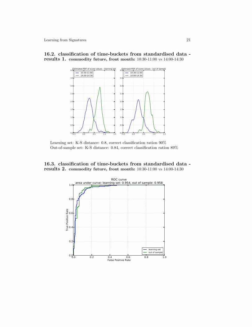
16.2. classification of time-buckets from standardised data -results 1. commodity future, front month: 10:30-11:00 vs 14:00-14:30
0.5 0.0 0.5 1.0 1.50.0
0.5
1.0
1.5
2.0
2.5
3.0
3.5
4.0Estimated PDF of score values - learning set
10:30-11:0014:00-14:30
0.5 0.0 0.5 1.0 1.50.0
0.5
1.0
1.5
2.0
2.5
3.0
3.5
4.0Estimaed PDF of score values - out of sample
10:30-11:0014:00-14:30
Learning set: K-S distance: 0.8, correct classification ration 90%Out-of-sample set: K-S distance: 0.84, correct classification ration 89%
16.3. classification of time-buckets from standardised data -results 2. commodity future, front month: 10:30-11:00 vs 14:00-14:30
0.0 0.2 0.4 0.6 0.8 1.0False Positive Rate
0.0
0.2
0.4
0.6
0.8
1.0
Tru
e P
osi
tive R
ate
ROC curvearea under curve: learning set: 0.954, out of sample: 0.958
learning set
out of sample
22 Terry Lyons
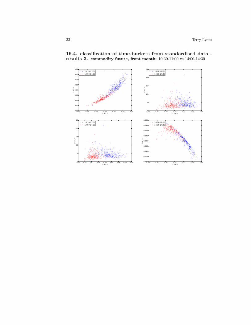
16.4. classification of time-buckets from standardised data -results 3. commodity future, front month: 10:30-11:00 vs 14:00-14:30
0.00 0.01 0.02 0.03 0.04 0.05 0.06(1,5,1,5)
0.00
0.01
0.02
0.03
0.04
0.05
0.06
0.07
0.08
(1,5
,5,5
)10:30-11:0014:00-14:30
0.00 0.01 0.02 0.03 0.04 0.05 0.06(1,5,1,5)
0
5
10
15
20
25
(6,2
,5,5
)
10:30-11:0014:00-14:30
0.00 0.01 0.02 0.03 0.04 0.05 0.06 0.07 0.08(1,5,5,5)
0
5
10
15
20
25
(6,2
,5,5
)
10:30-11:0014:00-14:30
0.00 0.01 0.02 0.03 0.04 0.05 0.06(1,5,1,5)
0.020
0.025
0.030
0.035
0.040
0.045
0.050
0.055
0.060
(5,1
,5,1
)
10:30-11:0014:00-14:30
Learning from Signatures 23
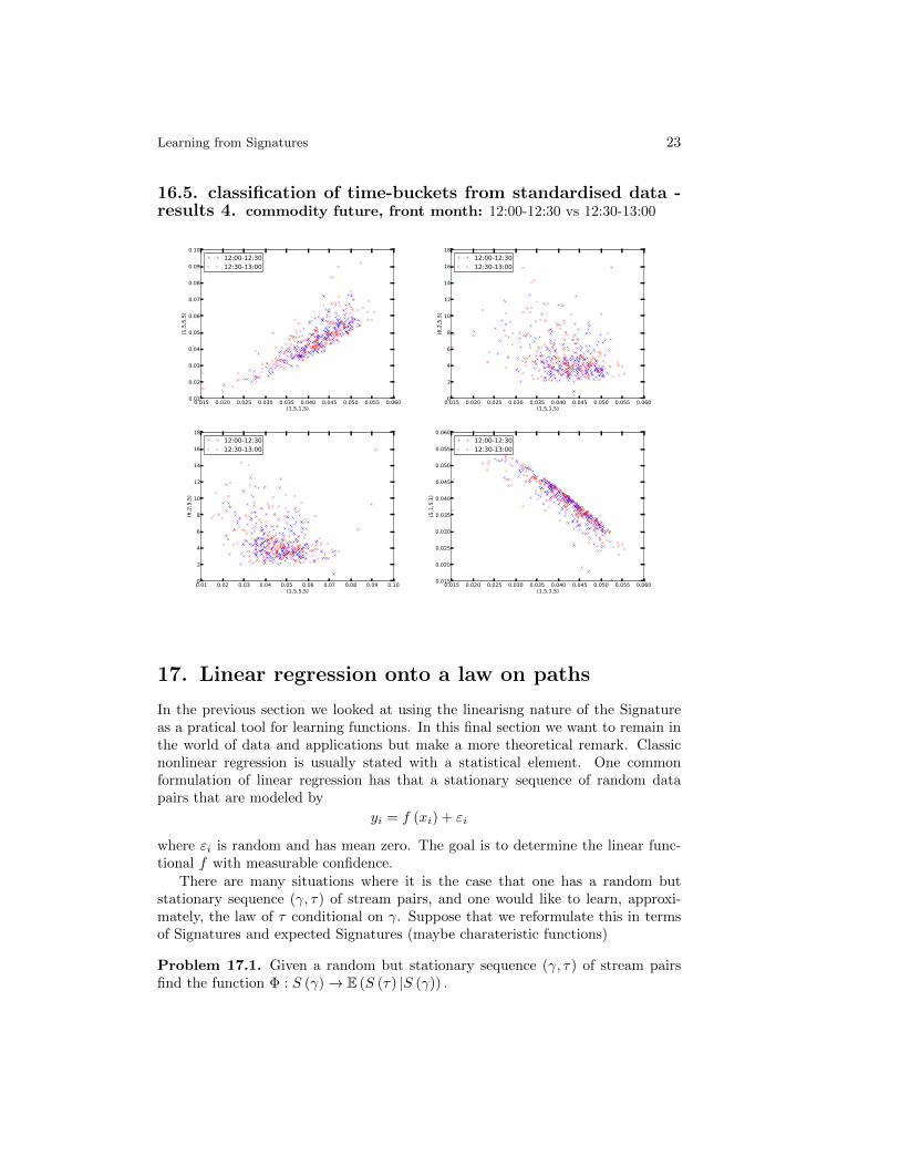
16.5. classification of time-buckets from standardised data -results 4. commodity future, front month: 12:00-12:30 vs 12:30-13:00
0.015 0.020 0.025 0.030 0.035 0.040 0.045 0.050 0.055 0.060(1,5,1,5)
0.01
0.02
0.03
0.04
0.05
0.06
0.07
0.08
0.09
0.10
(1,5
,5,5
)
12:00-12:3012:30-13:00
0.015 0.020 0.025 0.030 0.035 0.040 0.045 0.050 0.055 0.060(1,5,1,5)
0
2
4
6
8
10
12
14
16
18
(6,2
,5,5
)
12:00-12:3012:30-13:00
0.01 0.02 0.03 0.04 0.05 0.06 0.07 0.08 0.09 0.10(1,5,5,5)
0
2
4
6
8
10
12
14
16
18
(6,2
,5,5
)
12:00-12:3012:30-13:00
0.015 0.020 0.025 0.030 0.035 0.040 0.045 0.050 0.055 0.060(1,5,1,5)
0.015
0.020
0.025
0.030
0.035
0.040
0.045
0.050
0.055
0.060(5
,1,5
,1)
12:00-12:3012:30-13:00
17. Linear regression onto a law on paths
In the previous section we looked at using the linearisng nature of the Signatureas a pratical tool for learning functions. In this final section we want to remain inthe world of data and applications but make a more theoretical remark. Classicnonlinear regression is usually stated with a statistical element. One commonformulation of linear regression has that a stationary sequence of random datapairs that are modeled by
yi = f (xi) + εi
where εi is random and has mean zero. The goal is to determine the linear func-tional f with measurable confidence.
There are many situations where it is the case that one has a random butstationary sequence (γ, τ) of stream pairs, and one would like to learn, approxi-mately, the law of τ conditional on γ. Suppose that we reformulate this in termsof Signatures and expected Signatures (maybe charateristic functions)
Problem 17.1. Given a random but stationary sequence (γ, τ) of stream pairsfind the function Φ : S (γ)→ E (S (τ) |S (γ)) .
24 Terry Lyons
Then putting Yi = S (τi) and Xi = S (γi) we see that
Yi = Φ (Xi) + εi
where εi is random and has mean zero. If the measure is reasonably localisedand smooth then we can well approximate Φ by a polynomial and so to a linearfunction φ of the Signature. In other words the apparently difficult problem ofunderstanding conditional laws of paths becomes (at least locally) a problem oflinear regression
Yi = Φ (Xi) + εi
whch is infinite dimensional but which has well defined low dimensional approxi-mations [16].
References
[1] Horatio Boedihardjo, Uniqueness for the signature of sle curve, (2013).
[2] Nicolas Bourbaki, Lie groups and Lie algebras. Chapters 1–3, Elements of Mathe-matics (Berlin), Springer-Verlag, Berlin, 1989, Translated from the French, Reprintof the 1975 edition. MR 979493 (89k:17001)
[3] Youness Boutaib, Lajos Gergely Gyurko, Terry Lyons, and Danyu Yang, Dimension-free euler estimates of rough differential equations, to appear in Rev. RoumaineMath. Pures Appl. (2014).
[4] Thomas Cass and Terry Lyons, Evolving communities with individual preferences, toappear in Proceedings of London Mathematical Society (2014).
[5] Fabienne Castell and Jessica Gaines, An efficient approximation method for stochas-tic differential equations by means of the exponential lie series, Mathematics andcomputers in simulation 38 (1995), no. 1, 13–19.
[6] Kuo-Tsai Chen, Integration of paths, geometric invariants and a generalized Baker-Hausdorff formula, Ann. of Math. (2) 65 (1957), 163–178. MR 0085251 (19,12a)
[7] Ilya Chevyrev, Unitary representations of geometric rough paths, arXiv preprintarXiv:1307.3580 (2014).
[8] Wei-Liang Chow, Uber Systeme von linearen partiellen Differentialgleichungen ersterOrdnung, Math. Ann. 117 (1939), 98–105. MR 0001880 (1,313d)
[9] Thomas Fawcett, Problems in stochastic analysis: Connections between rough pathsand non-commutative harmonic analysis, Ph.D. thesis, University of Oxford, 2002.
[10] Guy Flint, Ben Hambly, and Terry Lyons, Convergence of sampled semimartingalerough paths and recovery of the it\ˆo integral, arXiv preprint arXiv:1310.4054v5(2013).
[11] Peter K Friz and Nicolas B Victoir, Multidimensional stochastic processes as roughpaths: theory and applications, vol. 120, Cambridge University Press, 2010.
[12] Lajos Gergely Gyurko, Terry Lyons, Mark Kontkowski, and Jonathan Field, Ex-tracting information from the signature of a financial data stream, arXiv preprintarXiv:1307.7244 (2013).

Learning from Signatures 25
[13] Martin Hairer, A theory of regularity structures, Invent. Math. (2014).
[14] Martin Hairer and Natesh S Pillai, Regularity of laws and ergodicity of hypoellipticsdes driven by rough paths, The Annals of Probability 41 (2013), no. 4, 2544–2598.
[15] Ben Hambly and Terry Lyons, Uniqueness for the signature of a path of boundedvariation and the reduced path group, Ann. of Math.(2) 171 (2010), no. 1, 109–167.
[16] Daniel Levin, Terry Lyons, and Hao Ni, Learning from the past, predicting thestatistics for the future, learning an evolving system, arXiv preprint arXiv:1309.0260(2013).
[17] Christian Litterer and Terry Lyons, Cubature on wiener space continued, StochasticProcesses and Applications to Mathematical Finance (2011), 197–218.
[18] Terry Lyons and Hao Ni, Expected signature of two dimensional Brownian Motionup to the first exit time of the domain, arXiv:1101.5902v4 (2011).
[19] Terry Lyons and Nicolas Victoir, Cubature on wiener space, Proceedings of the RoyalSociety of London. Series A: Mathematical, Physical and Engineering Sciences 460(2004), no. 2041, 169–198.
[20] Terry J Lyons, Michael Caruana, and Thierry Levy, Differential equations driven byrough paths, Springer, 2007.
[21] Terry J. Lyons and Nadia Sidorova, On the radius of convergence of the logarithmicsignature, Illinois J. Math. 50 (2006), no. 1-4, 763–790 (electronic). MR 2247845(2007m:60165)
[22] Terry J Lyons and Danyu Yang, The partial sum process of orthogonal expansionsas geometric rough process with fourier series as an examplean improvement ofmenshov–rademacher theorem, Journal of Functional Analysis 265 (2013), no. 12,3067–3103.
[23] P. K. Rashevski, About connecting two points of complete nonholonomic space byadmissible curve, Uch Zapiski ped. inst. Libknekhta 2 (1938), 83–94.
[24] Fei Yin, Qiu-Feng Wang, Xu-Yao Zhang, and Cheng-Lin Liu, Icdar 2013 chinesehandwriting recognition competition, Document Analysis and Recognition (ICDAR),2013 12th International Conference on, IEEE, 2013, pp. 1464–1470.
Oxford-Man Institute of Quantitative Finance, University of Oxford, England, OX26ED
E-mail: [email protected]