the geometry of the space of branched rough paths
TRANSCRIPT

THE GEOMETRY OF THE SPACE OF BRANCHED ROUGH PATHS
NIKOLAS TAPIA
WIAS-Institut Berlin, Mohrenstr. 39., 10117 Berlin, GermanyTechnische Universität Berlin, Str. des 17. Juni 136, 10587 Berlin, Germany.
LORENZO ZAMBOTTI
Laboratoire de Probabilités, Statistique et Modélisation, 4 place Jussieu, 75005 Paris,France
Abstract. We construct an explicit transitive free action of a Banach space of Hölderfunctions on the space of branched rough paths, which yields in particular abijectionbetween theses two spaces.This endows the space of branched rough paths with thestructure of a principal homogeneous space over a Banach space and allows to characterizeits automorphisms.The construction is based on the Baker-Campbell-Hausdorff formula,on a constructive version of the Lyons-Victoir extension theorem and on the Hairer-Kelly map, which allows to describe branched rough paths in terms of anisotropicgeometric rough paths.MSC (2010): 60H10; 16T05Keywords: Rough Paths; Hopf algebras;
Renormalisation
1. Introduction
The theory of Rough Paths has been introduced by Terry Lyons in the ’90s with the aimof giving an alternative construction of stochastic integration and stochastic differentialequations.More recently, it has been expanded by Martin Hairer to cover stochastic partialdifferential equations, with the invention of regularity structures.A rough path and a modelof a regularity structure are mathematical objects which must satisfy some algebraic andanalytical constraints.For instance, a rough path can be described as a Hölder functiondefined on an interval and taking values in a non-linear finite-dimensional Lie group;models of regularity structures are a generalization of this idea.A crucial ingredient ofregularity structures is the renormalisation procedure: given a family of regularized models,which fail to converge in an appropriate topology as the regularization is removed, onewants to modify it in a such a way that the algebraic and analytical constraints are stillsatisfied and the modified version converges.This procedure has been obtained in [6, 9]for a general class of models with a stationary character.The same question about roughpaths has been asked recently in [3, 4, 5], and indeed it could have been asked muchearlier.Maybe this has not happened because the motivation was less compelling; although
E-mail addresses: [email protected], [email protected]
arX
iv:1
810.
1217
9v5
[m
ath.
PR]
17
Nov
201
9

2 N. TAPIA AND L. ZAMBOTTI
one can construct examples of rough paths depending on a positive parameter which donot converge as the parameter tends to 0, this phenomenon is the exception rather thanthe rule.However the problem of characterizing the automorphisms of the space of roughpaths is clearly of interest; oneexample is the transformation from Itô to Stratonovichintegration, see e.g. [1, 16, 17]. However our aim is to put this particular example in amuch larger context.We recall that there are several possible notions of rough paths; inparticular we have geometric RPs and branched RPs, two notions defined respectivelyby Terry Lyons [29] and Massimiliano Gubinelli [25], see Sections 3 and 4 below.Thesetwo notions are intimately related to each other, as shown by Hairer and Kelly [28], seeSection 4 below.We note that regularity structures [27] are a natural and far-reachinggeneralization of branched RPs.In this paper we concentrate on the automorphisms ofthe space of branched RPs, see below for a discussion of the geometric case.Let F be thecollection of all non-planar rooted forests with nodes decorated by t1, . . . , du, see Section 4below.For instance the following forest
ab
ijk l
m
is an element of F. We call TĂ F the set of rooted trees, namely of non-empty forestswith a single connected component. Grading elements τ P F by the number |τ | of theirnodes we set
Tn – tτ P T : |τ | ď nu, n P N.Let now Hbe the linear span of F.It is possible to endow Hwith a product and a coproduct∆: HÑ HbHwhich make it a Hopf algebra, also known as the Butcher-Connes-KreimerHopf algebra, see Section 4.2 below.We let G denote the set of all characters over H, thatis, elements of G are functionals X P H˚ that are also multiplicative in the sense that
xX, τσy “ xX, τyxX, σy
for all forests (and in particular trees) τ, σ P F.Furthermore, the set G can be endowedwith a product ‹, dual to the coproduct, defined pointwise by xX ‹Y, τy “ xXbY,∆τy.Wework on the compact interval r0, 1s for simplicity, and all results canbe proved withoutdifficulty on r0, T s for any T ě 0.
Definition 1.1 (Gubinelli [25]). Given γ P s0, 1r, a branched γ-rough path is a pathX : r0, 1s2 Ñ Gwhich satisfies Chen’s rule
Xsu ‹Xut “ Xst, s, u, t P r0, 1s,and the analytical condition
|xXst, τy| À |t´ s|γ|τ |, τ P F.
Setting xit – xX0t, iy, t P r0, 1s, we say that X is a branched γ-rough path over the pathx “ px1, . . . , xdq. We denote by BRPγ the set of all branched γ-rough paths (for a fixedfinite alphabet t1, . . . , du).
By introducing the reduced coproduct ∆1 : HÑ HbH
∆1τ – ∆τ ´ τ b 1´ 1b τ,where 1 denotes the empty forest, Chen’s rule can we rewritten as follows
δxX, τysut “ xXsu bXut,∆1τy, s, u, t P r0, 1s, (1.1)
THE GEOMETRY OF THE SPACE OF BRANCHED ROUGH PATHS 3
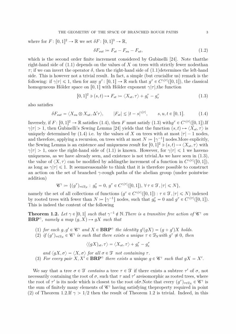
where for F : r0, 1s2 Ñ R we set δF : r0, 1s3 Ñ R,
δFsut – Fst ´ Fsu ´ Fut, (1.2)
which is the second order finite increment considered by Gubinelli [24]. Note thattheright-hand side of (1.1) depends on the values of X on trees with strictly fewer nodesthanτ ; if we can invert the operator δ, then the right-hand side of (1.1)determines the left-handside. This is however not a trivial result. In fact, a simple (but crucialfor us) remark is thefollowing: if γ|τ | ď 1, then for any gτ : r0, 1s Ñ R such that gτ P Cγ|τ |pr0, 1sq, the classicalhomogeneous Hölder space on r0, 1s with Hölder exponent γ|τ |,the function
r0, 1s2 Q ps, tq ÞÑ Fst – xXst, τy ` gτt ´ g
τs (1.3)
also satisfies
δFsut “ xXsu bXut,∆1τy, |Fst| À |t´ s|γ|τ |, s, u, t P r0, 1s. (1.4)
Inversely, if F : r0, 1s2 Ñ R satisfies (1.4), then F must satisfy (1.3) withgτ P Cγ|τ |pr0, 1sq.Ifγ|τ | ą 1, then Gubinelli’s Sewing Lemma [24] yields that the function ps, tq ÞÑ xXst, τy isuniquely determined by (1.4) i.e. by the values of X on trees with at most |τ | ´ 1 nodes,and therefore, applying a recursion, on trees with at most N – tγ´1u nodes.More explicitly,the Sewing Lemma is an existence and uniqueness result for r0, 1s2 Q ps, tq ÞÑ xXst, τy withγ|τ | ą 1, once the right-hand side of (1.1) is known. However, for γ|τ | ď 1 we havenouniqueness, as we have already seen, and existence is not trivial.As we have seen in (1.3),the value of xX, τy can be modified by addingthe increment of a function in Cγ|τ |pr0, 1sq,as long as γ|τ | ď 1. It seemsreasonable to think that it is therefore possible to constructan action on the set of branched γ-rough paths of the abelian group (under pointwiseaddition)
Cγ – tpgτ qτPTN : gτ0 “ 0, gτ P Cγ|τ |pr0, 1sq, @ τ P T, |τ | ď Nu,
namely the set of all collections of functions pgτ P Cγ|τ |pr0, 1sq : τ P T, |τ | ď Nq indexedby rooted trees with fewer than N – tγ´1u nodes, such that gτ0 “ 0 and gτ P Cγ|τ |pr0, 1sq.This is indeed the content of the following
Theorem 1.2. Let γ P s0, 1r such that γ´1 R N.There is a transitive free action of Cγ onBRPγ, namely a map pg,Xq ÞÑ gX such that
(1) for each g, g1 P Cγ and X P BRPγ the identity g1pgXq “ pg ` g1qX holds.(2) if pgτ qτPTN P Cγ is such that there exists a unique τ P TNwith gτ ı 0, then
xpgXqst, τy “ xXst, τy ` gτt ´ g
τs
and xgX, σy “ xX, σy for all σ P T not containing τ .(3) For every pair X,X 1 P BRPγ there exists a unique g P Cγ such that gX “ X 1.
We say that a tree σ P T contains a tree τ P T if there exists a subtree τ 1 of σ, notnecessarily containing the root of σ, such that τ and τ 1 areisomorphic as rooted trees, wherethe root of τ 1 is its node which is closest to the root ofσ.Note that every pgτ qτPTN P Cγ isthe sum of finitely many elements of Cγ having satisfying theproperty required in point(2) of Theorem 1.2.If γ ą 12 then the result of Theorem 1.2 is trivial. Indeed, in this

4 N. TAPIA AND L. ZAMBOTTI
case N “ 1, TN “ t i : i “ 1, . . . , du, andCγ “ tg i P Cγpr0, 1sq : g i0 “ 0, i “ 1, . . . , du.
Thenthe action is
pg,Xq ÞÑ gX, xpgXqst, iy– xXst, iy ` git ´ g
is , (1.5)
while the value of xgX, τy for |τ | ě 2 is uniquely determined by (1.1) via the SewingLemma. For example
xpgXqst, ijy–
ż t
s
pxju ´ xjs ` g
ju ´ g
js q dpxiu ` g i
u q, (1.6)
where xiu – xX0u, iy and the integral is well-defined in the Young sense, see [24, section3].If 13 ă γ ď 12 then N “ 2 and T2 “ T1 \ t i
j : i, j “ 1, . . . , du. Thenthe action atlevel |τ | “ 1 is still given by (1.5), while at level |τ | “ 2 we must have by (1.1)
δxgX,ijysut “ xpgXqsu b pgXqut,∆1τy “ pxju ´ x
js ` g
ju ´ g
js qpx
it ´ x
iu ` g
it ´ g
iu q. (1.7)
Although the right-hand side of (1.7) is explicit and simple, in this case there is nocanonicalchoice for xgX,
ijy. An expression like (1.6) is ill-defined in the Young sense, and the same
is true ifwe try the formulation
xpgXqst, ijy “ xXst, i
jy `
ż t
s
´
pxju ´ xjs ` g
ju ´ g
js q dg i
u ` pgju ´ g
js q dxiu
¯
, (1.8)
which satisfies formally (1.7), but the Young integrals are ill defined since2γ ď 1. Theconstruction of xgX,
ijy is therefore not trivial in this case.The same argument applies for
any γ ď 12 and any tree τ such that 2 ď |τ | ď N “ tγ´1u, and the fact that the aboveYoung integrals are not well defined shows why existence of the map X Ñ gX is nottrivial.Since Theorem 1.2 yields an action of Cγ on BRPγ which is regular, i.e. free andtransitive,then BRPγ is a principal Cγ-homogeneous space or Cγ-torsor. In particular,BRPγ is a copy of Cγ, but there is no canonical choice of an origin in BRPγ.Therefore,Theorem 1.2 also yields the following
Corollary 1.3. Given a branched γ-rough path X, the map g Ñ gX yields a bijectionbetween Cγ and the set of branched γ-rough paths.
Therefore Corollary 1.3 yields a complete parametrization of the space of branchedrough paths. This resultis somewhat surprising, since rough paths form a non-linear space,in particular because of the Chen relation; however Corollary 1.3 yields a natural bijectionbetween the space of branched γ-rough paths and thelinear space Cγ .Corollary 1.3 also givesa complete answer to the question of existence and characterization of branched γ-roughpaths over a γ-Hölder path x. Unsurprisingly, for our construction we start from a result ofT. Lyons and N. B. Victoir’s [30] of 2007, whichwas the first general theorem of existenceof a geometric γ-rough path over a γ-Hölder path x, see our discussion of Theorem 1.4below.An important point to stress is that the action constructed in Theorem 1.2 isneitherunique nor canonical. In the proof of Theorem 3.4 below, some parameters have tobe fixed arbitrarily,and the final outcome depends on them, see Remark 3.6. In this respect,the situation is similar to what happens in regularity structures with the reconstructionoperator on spaces Dγ with a negativeexponent γ ă 0, see [27, Theorem 3.10].

THE GEOMETRY OF THE SPACE OF BRANCHED ROUGH PATHS 5
1.1. Outline of our approach. A key point in Theorem 1.2 is the construction ofbranched γ-rough paths.In the case of geometric rough paths, see Definition 4.1, thesignature [11, 29] of a smooth path x : r0, 1s Ñ Rd yields a canonical construction. Othercases where geometric rough paths over non-smooth paths have been constructed areBrownian motion and fractional Brownian motion (see [13] for the case H ą 1
4 and [33]for the general case) among others.However, until T. Lyons and N. B. Victoir’s paper [30]in 2007, this question remained largely open in the general case.The precise result is asfollows
Theorem 1.4 (Lyons–Victoir extension). If p P r1,8qzN and γ : “ 1p, a γ-Hölder pathx : r0, 1s Ñ Rd can be lifted to a geometric γ-rough path. For any p ě 1 and ε P s0, γr, aγ-Hölder path can be lifted to a geometric pγ ´ εq-rough path.
Our first result is a version of this theorem which holds for rough paths in a moregeneral algebraic context, see Theorem 3.4 below. We use the Lyons-Victoir approachand an explicit form of the Baker–Campbell–Hausdorff formula by Reutenauer [34], seeformula (2.11) below. Whereas Lyons and Victoir used in one passage the axiom of choice,our method is completely constructive.Using the same idea we extend this construction tothe case where the collection px1, . . . , xdq is allowed to have different regularities in eachcomponent, which we call anisotropic (geometric) rough paths (aGRP), see Definition 4.8.
Theorem 1.5. To each collection pxiqi“1,...,d, with xi P Cγipr0, 1sq, we can associatean anisotropic rough path X over pxiqi“1,...,d. For every collection pgiqi“1,...,d, with gi PCγipr0, 1sq, denoting bygX the anisotropic geometric rough path over pxi ` giqi“1,...,d, wehave
g1pgXq “ pg ` g1qX.
This kind of extension to rough paths has already been explored in the papers [2, 26] inthe context of isomorphisms between geometric and branched rough paths.It turns outthat the additional property obtained by our method enables us to explicitly describethe propagation of suitable modifications from lower to higher degrees.We then go on todescribe the interpretation of the above results in the context of branched rough paths.The main tool is the Hairer–Kelly map [28], that we introduce and describein Lemma 5.1and then use to encode branched rough paths via anisotropic geometric rough paths, alongthe same lines as in [2, Theorem 4.3].
Theorem 1.6. Let X be a branched γ-rough path. There exists an anisotropic geometricrough path X indexed by words on the alphabet TN , with exponents pγτ “ γ|τ |, τ P TNq,and such that xX, τy “ xX, ψpτqy, where ψ is the Hairer–Kelly map.
The main difference of this result with [28, Theorem 1.9] is that we obtain an anisotropicgeometric rough path instead of a classical geometric rough path.This means that we do notconstruct unneeded components, i.e. components with regularity larger than 1, and we alsoobtain the right Hölder estimates in terms of the size of the indexing tree.This addresses twoproblems mentioned in Hairer and Kelly’s work, namely Remarks 4.14 and 5.9 in [28].Wethen use Theorem 1.5 and Theorem 1.6 to construct our action on branched roughpaths.

6 N. TAPIA AND L. ZAMBOTTI
Given pg,Xq P Cγ ˆBRPγ, we construct the anisotropic geometric roughpaths X andgX and then define the branched rough path gX P BRPγ as xgX, τy “ xgX, ψpτqy, whereψ is the Hairer–Kelly map.Our approach also does not make use of Foissy-Chapoton’sHopf-algebra isomorphism [10, 20] between the Butcher–Connes–Kreimer Hopf algebraand the shuffle algebra over a complicated set I of trees as is done in [2].This allows us toconstruct an action of a larger group on the set of branched rough paths;indeed, usingthe above isomorphism one would obtain a transformation group parametrized by pgτ qτPIwhere I is the aforementioned set of trees of Foissy-Chapoton’s results and gτ P Cγ|τ |;onthe other hand our approach yields a transformation group parametrized by pgτ qτPTN .With the smaller set I XTN , transitivity of the action g ÞÑ gX would be lost.Finally wenote that we use a special property of the Butcher-Connes-Kreimer Hopf algebra: the factthat it is freelygenerated as an algebra by the set of trees, so defining characters over itis significantly easier than in the geometric case.To define an element X P G it sufficesto give the values xX, τy for all trees τ P T; by freeness there is a unique multiplicativeextension to all of H.This is not at all the case for geometric rough paths: the shufflealgebra T pAq over an alphabet A is not free over the linear span of words so if one iswilling to define a character X over T pAq there are additional algebraic constraints thatthe values of X on words must satisfy.
Outline. We start by reviewing all the theoretical concepts needed to make the expositionin this section formal.In Section 3 we state and prove the main result of this chapter. Weextend the notion of rough path and we give an explicit construction of such a generalizedrough path above any given path x P Cγ.Next, in Section 4.3 we extend this resultto the class of anisotropic geometric rough paths.Finally, in Section 4 we connect ourconstruction with M. Gubinelli’s branched rough paths, and we extend M. Hairer and D.Kelly’s work in Section 5.1.We also explore possible connections with renormalisation inSection 6 by studying how our construction behaves under modification of the underlyingpaths.Then, we connect this approach with a recent work by Bruned, Chevyrev, Friz andPreiß [4] in Section 6.1, who borrowed ideas from the theory of Regularity Structures[6, 27] and proposed a renormalisation procedure for geometric and branched rough paths[4]based on pre-Lie morphisms.The main difference between our result and the BCFPprocedure is that they consider translation only by time-independent factors, whereas–under reasonable hypotheses– we are also able to handle general translations depending onthe time parameter.We also mention that some further algebraic aspects of renormalisationin rough paths have been recently developed in [5].
Acknowledgements. The authors thank Jean-David Jacques for pointing out a mistakein a previous version.N.T. acknowledges support by the CONICYT/Doctorado Nacionaldoctoral scholarship grant number 2013-21130733, Núcleo Milenio Modelos Estocásticos deSistemas Complejos y Desordenados and the Berlin Mathematical School MATH+ EF1-5project “On robustness of deep neural networks”. L.Z. gratefully acknowledges support bythe project of the Agence Nationale de la Recherche ANR-15-CE40-0020-01 grant LSD.

THE GEOMETRY OF THE SPACE OF BRANCHED ROUGH PATHS 7
2. Preliminaries
A Hopf algebra H is a vector space endowed with an associative product m : HbHÑ H:mpmb idq “ mpidbmq,
and a coassociative coproduct ∆: HÑ HbH:pidb∆q∆ “ p∆b idq∆,
satisfying moreover certain compatibility assumptions; H is also supposed to have a unit1 P H, a counit ε P H˚ and an antipode S : HÑ H such that
mpidb Sq∆x “ εpxq1 “ mpS b idq∆xfor all x P H.As usual we will use the more compact notation mpxb yq “ xy.The readeris referred to the papers [8, 31] for further details.
Definition 2.1. We say that the Hopf algebra H is graded if it can be decomposed as adirect sum
H“
8à
n“0Hpnq (2.1)
withm : Hpnq bHpmq Ñ Hpn`mq, ∆: Hpnq Ñ
à
p`q“n
Hppq bHpqq. (2.2)
In a graded Hopf algebra, each element x P H can be decomposed as a sum
x “8ÿ
n“0xn, xn P Hpnq, (2.3)
where only a finite number of the summands are non-zero.We call each xn the homogeneouspart of degree n of x, and elements of Hpnq are said to be homogeneous of degree n.In thiscase we write |xn| “ n.
Definition 2.2. The graded Hopf algebra H is connected if the degree 0 part is one-dimensional. It is locally finite if dim Hpnq ă 8 for all n ě 0.
From now on we consider a graded connected locally finite Hopf algebra H.Then, forany homogeneous element x P Hpnq the coproduct can be written as
∆x “ xb 1` 1b x`∆1x, where ∆1x Pà
p`q“np,qě1
Hppq bHpqq
and ∆1 : HÑ HbH is known as the reduced coproduct.Furthermore, the coassociativityof ∆ and of ∆1, i.e. the identity p∆1b idq∆1 “ pidb∆1q∆1, allows to unambiguously definetheir iterates ∆n,∆1
n : HÑ Hbpn`1q by setting for n ě 2∆n “ pidb∆n´1q∆, ∆1
n “ pidb∆1n´1q∆1.
Then we have, for a homogeneous element x P Hpkq of degree k,
∆1nx P
à
p1`...`pn`1“kpjě1
Hpp1q b ¨ ¨ ¨ bHppn`1q.

8 N. TAPIA AND L. ZAMBOTTI
Remark 2.3. These properties of the iterated coproduct imply that the bialgebra pH,∆qis conilpotent, that is, for each homogeneous x P Hpkq there is an integer n ď k suchthat∆1
nx “ 0.We obtain also the inclusion
∆1nHpn`1q Ă H
bpn`1qp1q ,
that is, the n-fold reduced coproduct of a homogeneous element of degree n` 1 is a sumof pn` 1q-fold tensor products of homogeneous elements of degree 1.
We recall that in general the dual space H˚ carries an algebra structure given by theconvolution product ‹, dual to the coproduct ∆, defined by
xf ‹ g, xy– xf b g,∆xy.
For a collection of maps f1, . . . , fk P H˚ we have the formula
f1 ‹ ¨ ¨ ¨ ‹ fk “ pf1 b ¨ ¨ ¨ b fkq ˝∆k´1. (2.4)
Definition 2.4. A character on H is a non-zero linear map X : HÑ R
xX, xyy “ xX, xyxX, yy, @x, y P H.
for all x, y P H. We call G the set of all characters on H.An infinitesimal character (orderivation) on H is a linear map α : HÑ R such that
xα, xyy “ xα, xyxε, yy ` xε, xyxα, yy, @x, y P H.
We call g the set of all infinitesimal characters on H.
We observe that necessarily xX,1y “ 1 and xα,1y “ 0 for all X P G and α P g.It iswell known that the pG, ‹, εq is a group with product ‹, unit ε and inverse X´1 “ X ˝ Swhere S is the antipode defined above.Moreover pg, r¨, ¨sq is a Lie algebra with bracketrα, βs– α ‹ β ´ β ‹ α.See e.g. [31].
2.1. Nilpotent Lie algebras. From (2.2) we have
Lemma 2.5. For any N P N the subspace
HN –
Nà
k“0Hpkq Ă H
is a counital subcoalgebra of pH,∆, εq.
By Lemma 2.5 we can consider the dual algebra pH˚N , ‹, εq.This algebra is also graded
and connected, since we have the natural grading
H˚N “
Nà
k“0H˚pkq, H˚
N Q α “Nÿ
k“0αpkq, (2.5)
where αpkq : HN Ñ R is defined by αpkqpxq – αpxkq with the notation (2.3).Since HN isnot a subalgebra of H, the notions of character and infinitesimal character on H˚
N are notwell-defined. We can however introduce their truncated versions.

THE GEOMETRY OF THE SPACE OF BRANCHED ROUGH PATHS 9
Definition 2.6. We say that X P H˚Nzt0u is a truncated character on HN if
xX, xyy “ xX, xyxX, yy
holds for all x P Hpnq, y P Hpmq with n ` m ď N . We call GN the space of truncatedcharacters on HN .Likewise, we say that α P H˚
N is a truncated infinitesimal character if
xα, xyy “ xα, xyxε, yy ` xε, xyxα, yy
holds for all x P Hpnq, y P Hpmq with n `m ď N . We call gN the space of truncatedin-finitesimal characters on HN .
Lemma 2.7. There are a canonical inclusions H˚N ãÑ H˚
N`1 ãÑ H˚, which induce canonicalinclusion gN ãÑ gN`1 ãÑ g. Moreover such canonical inclusions are right-inverse forthecorresponding restriction maps H˚ Ñ H˚
N`1 Ñ H˚N .
Proof. Using the notation (2.5), we can extend α P H˚N to α P H˚
N`1 (respectively H˚) bysetting αpN`1q ” 0 (respectively αpkq ” 0 for all k ě N ` 1).Trivially this extension takesH˚N to H˚
N`1. If α P gN and x, y P HN are such that |x| ` |y| ď N ` 1 then
xα, xyy “A
α,N`1ÿ
j“0pxyqj
E
“
Nÿ
j“0xα, pxyqjy “
Nÿ
j“0
jÿ
k“0xα, xkyk´jy
“
Nÿ
j“0pxα, xjyxε, yy ` xε, xyxα, yjyq “ xα, xyxε, yy ` xε, xyxα, yy.
so that the extension of α is in gN`1.The same argument yields the inclusion gN ãÑ g.
There are also the truncated exponential expN : H˚N Ñ H˚
N and logarithm logN : H˚N Ñ
H˚N , defined by the sums
expNpαq–Nÿ
k“0
1k! α
‹kˇ
ˇ
HN, logNpXq–
Nÿ
k“1
p´1qk`1
kpX ´ εq‹k
ˇ
ˇ
HN. (2.6)
The proof of the next result can be found for instance in [19, Thm 77].
Lemma 2.8. pGN , ‹, εq is a group and pgN , r¨, ¨sq is a Lie algebra.Moreover, expN : gN ÑGN is a bijection with inverse logN : GN Ñ gN .
For every k ě 0 we define now, using the notation (2.5),
Wk –
α P g : α “ αpkq(
.
Lemma 2.9. For all n,m ě 0 we have rWn,Wms Ă Wn`m.
Proof. Let x P H. With the notation (2.3) we have for α P Wn and β P Wm
pα ‹ β ´ β ‹ αqpxq “ pα b β ´ β b αq∆x “ pα b β ´ β b αq∆xn`mby (2.2).

10 N. TAPIA AND L. ZAMBOTTI
By the canonical inclusion of Lemma 2.7, we observe that
gN “Nà
k“1Wk, gN Q α “
Nÿ
k“0αpkq (2.7)
in the notation (2.5).With this decomposition gN becomes by Lemma 2.9 a graded Liealgebra.We recall that the center of gN is the subspace of all w P gN such that rα,ws “ 0for all α P gN ,while the center of GN is the set of all X P GN such that X ‹ Y “ Y ‹Xfor all Y P GN .
Proposition 2.10. WN is contained in the center of gN and expNpWNq is a subgroupcontained in the center of GN .
Proof. Let α P gN and w P WN . Clearly, xrα,ws, xy is zero unless |x| “ N .In this casexrα,ws, xy “ xα b w ´ w b α,∆xy “ xα, 1yxw, xy ´ xw, xyxα, 1y “ 0
since xw, yy “ xw, yNy, in the notation (2.3). The second assertion follows easily: it isenough to write X “ expNpwq and Y “ expNpαq with α P gN and w P WN and use theexplicit representation (2.6) of expN and the fact that α ‹ w “ w ‹ α.
The next (famous) result describes the group law on GN in terms of an operation ongN via the exponential/logarithmic map.
Theorem 2.11 (Baker–Campbell–Hausdorff). For all α, β P gN , we havelogNpexpNpαq ‹ expNpβqq P gN .
We define the map BCHN : gN ˆ gN Ñ gN byBCHNpα, βq– logNpexpNpαq ‹ expNpβqq. (2.8)
Another way to interpret this theorem is to say that there exists an element γ “
BCHNpα, βq P gN such that expNpαq ‹ expNpβq “ expNpγq.It is a classical result that themap BCHN is formed by a sum of iterated Lie brackets of α and β, where the first termsare
BCHNpα, βq “ α ` β `12rα, βs `
112rα, rα, βss ´
112rβ, rα, βss ` ¨ ¨ ¨ , (2.9)
and the following ones are explicit but difficult to compute.Nevertheless, fully explicitformulas have been known since 1947 by Dynkin [15].For our purposes, however, Dynkin’sformula is too complicated (for example, the regularity argument in step 2 of the proof ofTheorem 3.4 would not be as evident) so we rely on a different expression first shown byReutenauer [34].In order to describe it, let ϕk : pH˚qbk Ñ H˚ be the linear map
ϕkpα1 b ¨ ¨ ¨ b αkq “ÿ
σPSk
aσ ασp1q ‹ ¨ ¨ ¨ ‹ ασpkq (2.10)
where Sk denotes the symmetric group of order k, and aσ –p´1qdpσq
k
`
k´1dpσq
˘´1 is a constantdepending only on the descent number dpσq of the permutation σ P Sk, namely the numberof i P t1, . . . , k ´ 1u such that σpiq ą σpi` 1q.

THE GEOMETRY OF THE SPACE OF BRANCHED ROUGH PATHS 11
Lemma 2.12 (Reutenauer’s formula). For all α, β P gN
BCHNpα, βq “Nÿ
k“1
ÿ
i`j“k
1i!j! ϕkpα
bib βbjq. (2.11)
Moreover, for all i P t0, . . . , Nu, we have ϕN`
αbi b βbpN´iq˘
P WN .
Proof. Let us suppose first that T pV q is the (completed) tensor algebra over a two-dimensional vector space V ,with V linearly generated by te1, e2u. Then the result iscontained in Reutenauer’s paper [34] where the free step-N nilpotent Lie algebra LN playsthe rôle of gN .We want now to show how this implies the same result in our more generalsetting.Let α, β P gN and let Φ: pT pV qN ,bq Ñ pH˚
N , ‹q be the unique algebra morphismsuch thatΦpe1q “ α, Φpe2q “ β. Then Φ restricts to a Lie-algebra morphism Φ: LN Ñ gN
such that BCHNpα, βq “ ΦpBCHNpe1, e2qq and therefore (2.11) follows.In order to provethe first formula, we first note that Φ is not a graded morphism, since the generators e1 ande2 are homogeneous of degree 1 in T pV qN , but α and β are in general not homogeneous inH˚N .However, from the bilinearity of the Lie bracket and Lemma 2.9 we obtain
rWn ‘ ¨ ¨ ¨ ‘WN ,Wm ‘ ¨ ¨ ¨ ‘WN s Ă Wn`m ‘Wn`m`1 ‘ ¨ ¨ ¨ ‘WN .
Then, if α1, . . . , αk P gN then ϕkpα1 b ¨ ¨ ¨ b αkq P Wk ‘ ¨ ¨ ¨ ‘WN .
From all these considerations we obtain the following result on the map
BCHpn`1q : gn`1ˆ gn`1
Ñ Wn`1, BCHpn`1q – BCHn`1´BCHn, n ě 0. (2.12)
Note that BCHpn`1q takes indeed values in Wn`1 rather than in gn`1 by (both assertionsof)Lemma 2.12.
Lemma 2.13. Let x P Hpn`1q and α, β P gn`1. Then
xBCHpn`1qpα, βq, xy “ÿ
i`j“n`1
1i!j!
ÿ
pxq
ÿ
σPSn`1
aσ
iź
p“1xα, xpσ´1ppqqy
n`1ź
q“i`1xβ, xpσ´1pqqqy, (2.13)
where∆1nx “
ÿ
pxq
xp1q b ¨ ¨ ¨ b xpn`1q P Hbpn`1qp1q .
Proof. Set α1 “ ¨ ¨ ¨ “ αi – α, αi`1 “ ¨ ¨ ¨ “ αn`1 – β.Then the result follows directlyfrom the definition of ϕk in (2.10) together with (2.4) and the fact that since xαj,1y “ 0we can write
α1 ‹ ¨ ¨ ¨ ‹ αn`1 “ pα1 b ¨ ¨ ¨ b αn`1q∆1n (2.14)
instead (note the reduced coproduct in place of the full coproduct).
12 N. TAPIA AND L. ZAMBOTTI
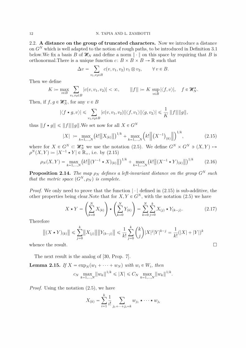
2.2. A distance on the group of truncated characters. Now we introduce a distanceon GN which is well adapted to the notion of rough paths, to be introduced in Definition 3.1below.We fix a basis B of HN and define a norm ¨ on this space by requiring that B isorthonormal.There is a unique function c : B ˆB ˆB Ñ R such that
∆v “ÿ
v1,v2PB
cpv, v1, v2q v1 b v2, @ v P B.
Then we defineK – max
vPB
ÿ
v1,v2PB
|cpv, v1, v2q| ă 8, ~f~– K supvPB
|xf, vy|, f P H˚N .
Then, if f, g P H˚N , for any v P B
|xf ‹ g, vy| ďÿ
v1,v2PB
|cpv, v1, v2q||xf, v1y||xg, v2y| ď1K~f~~g~,
thus ~f ‹ g~ ď ~f~~g~.We set now for all X P GN
|X| – maxk“1,...,N
`
k!
Xpkq
˘1k` max
k“1,...,N
´
k!
`
X´1˘
pkq
¯1k, (2.15)
where for X P GN Ă H˚N we use the notation (2.5). We define GN ˆ GN Q pX, Y q ÞÑ
ρNpX, Y q– |X´1 ‹ Y | P R`, i.e. by (2.15)
ρNpX, Y q “ maxk“1,...,N
`
k!
pY ´1‹Xqpkq
˘1k` max
k“1,...,N
`
k!
pX´1‹ Y qpkq
˘1k (2.16)
Proposition 2.14. The map ρN defines a left-invariant distance on the group GN suchthat the metric space pGN , ρNq is complete.
Proof. We only need to prove that the function | ¨ | defined in (2.15) is sub-additive, theother properties being clear.Note that for X, Y P GN , with the notation (2.5) we have
X ‹ Y “
˜
Nÿ
k“0Xpkq
¸
‹
˜
Nÿ
k“0Ypkq
¸
“
Nÿ
k“0
kÿ
j“0Xpjq ‹ Ypk´jq. (2.17)
Therefore
pX ‹ Y qpkq
ď
kÿ
j“0
Xpjq
Ypk´jq
ď1k!
kÿ
j“0
ˆ
k
j
˙
|X|j|Y |k´j “1k!p|X| ` |Y |q
k
whence the result.
The next result is the analog of [30, Prop. 7].
Lemma 2.15. If X “ expNpw1 ` ¨ ¨ ¨ ` wNq with wi P Wi, then
cN maxk“1,...,N
~wk~1kď |X| ď CN max
k“1,...,N~wk~
1k.
Proof. Using the notation (2.5), we have
Xpkq “kÿ
i“1
1i!
ÿ
j1`¨¨¨`ji“k
wj1 ‹ ¨ ¨ ¨ ‹ wji
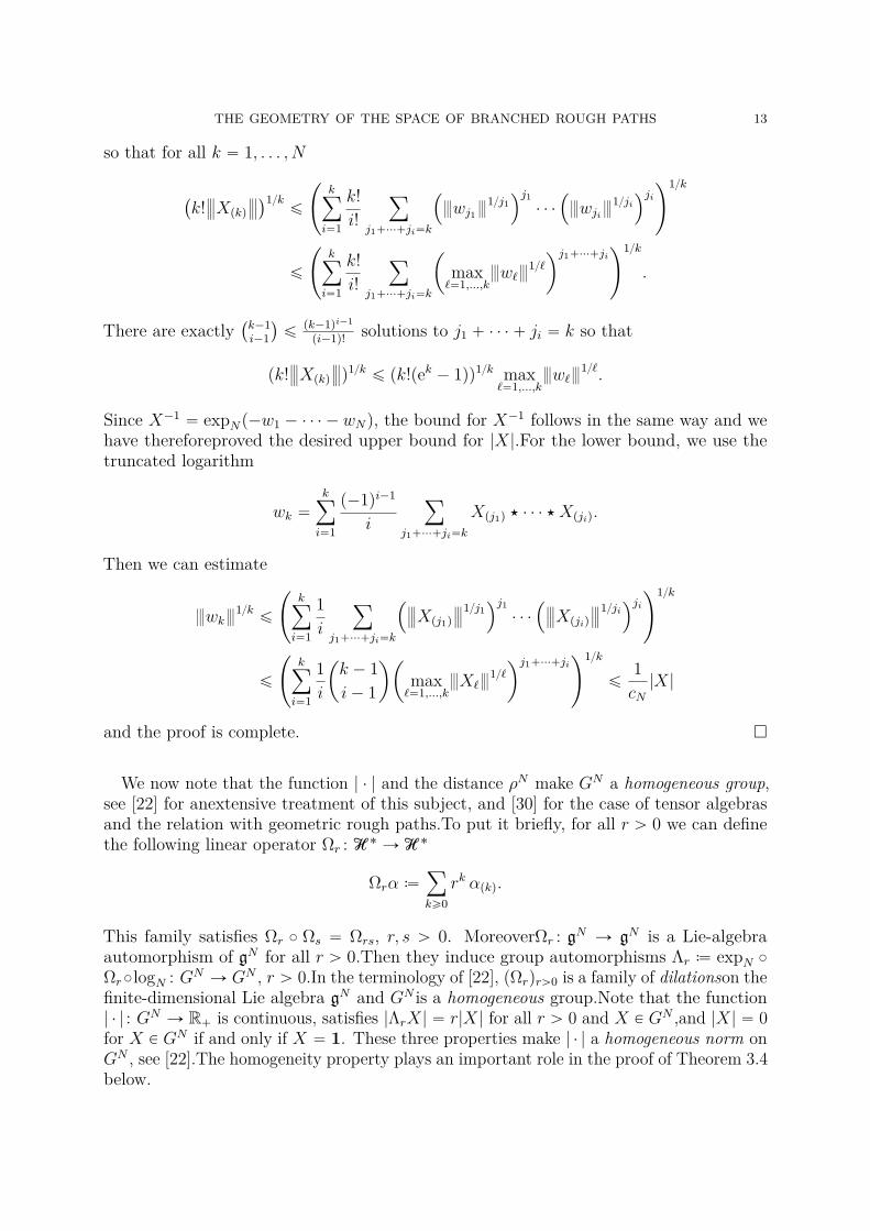
THE GEOMETRY OF THE SPACE OF BRANCHED ROUGH PATHS 13
so that for all k “ 1, . . . , N
`
k!
Xpkq
˘1kď
˜
kÿ
i“1
k!i!
ÿ
j1`¨¨¨`ji“k
´
~wj1~1j1
¯j1¨ ¨ ¨
´
~wji~1ji
¯ji
¸1k
ď
˜
kÿ
i“1
k!i!
ÿ
j1`¨¨¨`ji“k
ˆ
max`“1,...,k
~w`~1`˙j1`¨¨¨`ji
¸1k
.
There are exactly`
k´1i´1
˘
ďpk´1qi´1
pi´1q! solutions to j1 ` ¨ ¨ ¨ ` ji “ k so that
pk!
Xpkq
q1kď pk!pek ´ 1qq1k max
`“1,...,k~w`~
1`.
Since X´1 “ expNp´w1 ´ ¨ ¨ ¨ ´ wNq, the bound for X´1 follows in the same way and wehave thereforeproved the desired upper bound for |X|.For the lower bound, we use thetruncated logarithm
wk “kÿ
i“1
p´1qi´1
i
ÿ
j1`¨¨¨`ji“k
Xpj1q ‹ ¨ ¨ ¨ ‹Xpjiq.
Then we can estimate
~wk~1kď
˜
kÿ
i“1
1i
ÿ
j1`¨¨¨`ji“k
´
Xpj1q
1j1¯j1¨ ¨ ¨
´
Xpjiq
1ji¯ji
¸1k
ď
˜
kÿ
i“1
1i
ˆ
k ´ 1i´ 1
˙ˆ
max`“1,...,k
~X`~1`˙j1`¨¨¨`ji
¸1k
ď1cN|X|
and the proof is complete.
We now note that the function | ¨ | and the distance ρN make GN a homogeneous group,see [22] for anextensive treatment of this subject, and [30] for the case of tensor algebrasand the relation with geometric rough paths.To put it briefly, for all r ą 0 we can definethe following linear operator Ωr : H˚ Ñ H˚
Ωrα –ÿ
kě0rk αpkq.
This family satisfies Ωr ˝ Ωs “ Ωrs, r, s ą 0. MoreoverΩr : gN Ñ gN is a Lie-algebraautomorphism of gN for all r ą 0.Then they induce group automorphisms Λr – expN ˝Ωr˝logN : GN Ñ GN , r ą 0.In the terminology of [22], pΩrqrą0 is a family of dilationson thefinite-dimensional Lie algebra gN and GN is a homogeneous group.Note that the function| ¨ | : GN Ñ R` is continuous, satisfies |ΛrX| “ r|X| for all r ą 0 and X P GN ,and |X| “ 0for X P GN if and only if X “ 1. These three properties make | ¨ | a homogeneous norm onGN , see [22].The homogeneity property plays an important role in the proof of Theorem 3.4below.

14 N. TAPIA AND L. ZAMBOTTI
3. Construction of Rough paths
As in the previous section, we fix a locally-finite graded connected Hopf algebra H.We alsofix a number γ P s0, 1r and let N – tγ´1u be the biggest integer such that Nγ ď 1.Withoutloss of generality we can fix a basis B of HN consisting only of homogeneous elements andin particular we let te1, . . . , edu “ B XHp1q where d– dim Hp1q.Definition 3.1. A pH, γq-rough path is a function X : r0, 1s2 Ñ GN , with N “ tγ´1u,which satisfies Chen’s rule
Xsu ‹Xut “ Xst, s, u, t P r0, 1s, (3.1)and such that for all v P B
|xXst, vy| À |t´ s|γ|v|. (3.2)
If xi : r0, 1s Ñ R, i “ 1, . . . , d, is such thatxit ´ xis “ xXst, eiy, s, t P r0, 1s, we say that Xis a γ-rough path over px1, . . . , xdq.Remark 3.2. By specializing this definition to different choices of H we recover bothgeometric rough paths [29] where H is the shuffle Hopf algebra over an alphabet, branchedrough paths [25] where H is the Butcher–Connes–Kreimer Hopf algebra on decoratednon-planar rooted trees, and also planarly branched rough paths [14].
We remark that there is a bijection between
(1) functions X : r0, 1s2 Ñ GN such that Xsu ‹Xut “ Xst, for all s, u, t P r0, 1s,(2) functions X : r0, 1s Ñ GN such that X0 “ 1,
given byX ÞÑ X, Xt – X0t, X ÞÑ X, Xst – X´1
s ‹ Xt, s, t P r0, 1s. (3.3)Proposition 3.3. Let X : r0, 1s Ñ GN and X : r0, 1s2 Ñ GN as in (3.3).Then X is apH, γq-rough path as in Definition 3.1 if and only if X is γ-Hölder with respect to themetric ρN defined in (2.15).
Proof. First note that the distance in (2.16) is defined with respect to a fixed (but arbitrary)basis so we use the basis B fixed at the beginning of this section.Also, due to the aboveremark we only have to verify that X is γ-Hölder with respect to ρN if and only if Xsatisfies (3.2) using the same basis.In one direction, if X is γ-Hölder then, by definition
|Xst| “ ρNpXs,Xtq À |t´ s|γ
and so, for a basis element v P B we have|xXst, vy| À |t´ s|
γ|v|.
Conversely, if (3.2) holds then |Xst| À |t´s|γ and so by definition also ρNpXs,Xtq À |t´s|
γ ,i.e. X is γ-Hölder with respect to ρN .
We now come to the problem of existence.Our construction of a rough path in the senseof Definition 3.1 over an arbitrary collection of γ-Hölder paths px1, . . . , xdq relies in thefollowing extension theorem. We note that theproof is a reinterpretation of the approachof Lyons-Victoir [30, Theorem 1] in the context of a more general graded Hopf-algebra H.

THE GEOMETRY OF THE SPACE OF BRANCHED ROUGH PATHS 15
Theorem 3.4 (Rough path extension). Let 1 ď n ď N ´ 1 and γ P s0, 1r such thatγ´1 R N. Suppose we have a γ-Hölder path Xn : r0, 1s Ñ pGn, ρnq.There is a γ-Hölder pathXn`1 : r0, 1s Ñ pGn`1, ρn`1q extending Xn, i.e. such that Xn`1|Hn “ Xn.
A key tool is the following technical lemma whose proof can be found in [30, Lemma 2].Lemma 3.5. Let pE, ρq be a complete metric space and set
D “ ttmk – k2´m : m ě 0, k “ 0, . . . , 2m ´ 1u.Suppose y : D Ñ E is a path satisfying the bound ρpytm
k, ytm
k`1q À 2´γm for some γ P
p0, 1q.Then, there exists a γ-Hölder path x : r0, 1s Ñ E such that x|D “ y.
Proof of Theorem 3.4. The construction of Xn`1 is made in two steps.
Step 1. For m ě 0 and k P t0, . . . , 2mu we define tmk – k2´m P r0, 1s. Then we define thefollowing sets of dyadics in r0, 1s
Dpmq – ttmk | k “ 0, . . . , 2mu, Dm –ď
n“0,...,mDpnq, D –
ď
mě0Dpmq.
Set Xst “ pXns q´1 ‹Xn
t P Gn and Lst “ lognpXstq P g
n where logn was defined in (2.6).Then,the Baker–Campbell–Hausdorff formula (2.8) and Chen’s rule (3.1) imply that
Lst “ BCHnpLsu, Lutq. (3.4)We look for Y : r0, 1s2 Ñ Gn`1 such that Y satisfies Chen’s rule (3.1) andY
ˇ
ˇ
HN“ X.
We usethroughout the proof that gn Ă gn`1, see Lemma 2.7.In a first step, we defineY : D ˆD Ñ Gn`1. In the second step we show that Y has suitable uniformcontinuityproperties and can thus be extended to r0, 1s2 using Lemma 3.5.The construction ofY : D ˆD Ñ Gn`1 goes through a construction of Y m : Dm ˆDm Ñ Gn`1 by recursionon m ě 0.We claim that for all m ě 0 we can find Y m such that
(1) Y m satisfies Chen’s relation on Dm, namelyY mab ‹ Y
mbc “ Y m
ac for all a, b, c P Dm
(2) for any n P t0, . . . ,mu and k, ` P t0, . . . , 2m´nu, we have the compatibility relationY mtmk2n t
m`2n“ Y m´n
tm´nk
tm´n`
.
(3) Y m restricted to Hn is equal to X : Dm ˆDm Ñ Gn, in the sense thatY mab |Hn “ Xab, @ a, b P Dm.
(4) for all k “ 0, . . . , 2m ´ 1, setting
Zmtmktmk`1
– logn`1
´
Y mtmktmk`1‹ expn`1
´
´Ltmktmk`1
¯¯
,
we have Zmtmktmk`1P Wn`1.
For m “ 0, we setY 001 “ expn`1pL01q, Y 0
00 “ Y 011 – ε, and Z0
01 – 0 P Wn`1. Forx P Hn,we have xexpn`1pL01q, xy “ xexpnpL01q, xy, so that Y 0 restricted to Hn is equalto X : D0 ˆ D0 Ñ Gn.Let now m ě 1, and suppose that Y m´1 : Dm´1 ˆ Dm´1 Ñ Gn`1
has been constructed with the above properties.We start by defining Y mtt “ ε for all
t P Dpmq.Let us consider three consecutive points in Dpmq of the forms “ tm2k, u “ tm2k`1, t “ tm2k`2

16 N. TAPIA AND L. ZAMBOTTI
for some k “ 0, . . . , 2m´1´1. Note that s “ tm´1k and t “ tm´1
k`1 , so that Zmst – Zm´1
st P Wn`1is already defined by the recurrence hypothesis. We define Zm
su and Zmut as follows
Zmsu “ Zm
ut –12`
Zm´1st ´ BCHpn`1qpLsu, Lutq
˘
, (3.5)
where BCHpn`1q “ BCHn`1´BCHn : gn`1ˆgn`1 Ñ Wn`1, see (2.12). Since by recurrenceZm´1st P Wn`1, we obtain that Zm
su, Zmut P Wn`1 and
Zmsu ` Z
mut “ Zm´1
st ´ BCHpn`1qpLsu, Lutq “ Lst ` Zmst ´ BCHn`1pLsu, Lutq (3.6)
where in the last equality we have applied (3.4). Then we set
Y msu – expn`1pLsu ` Z
msuq, Y m
ut – expn`1pLut ` Zmutq.
Since expn`1pWn`1q is in the center of Gn`1 by Proposition 2.10, we obtain that
Y msu “ expn`1pLsuq ‹ expn`1pZ
msuq, Y m
ut “ expn`1pLutq ‹ expn`1pZmutq.
By (2.8) and (3.6) the product is equal to
Y msu ‹ Y
mut “ expn`1pBCHn`1pLsu, Lutq ` Z
msu ` Z
mutq “ expn`1pLst ` Z
mst q “ Y m
st .
Let now tmj , tmk P Dpmq with 0 ď j ă k ď 2m.We set
Y mtmj t
mk– Y m
tmj tmj`1‹ ¨ ¨ ¨ ‹ Y m
tmk´1t
mk, Y m
tmktmj
–
´
Y mtmj t
mk
¯´1
so that the identity Y mab ‹ Y
mbc “ Y m
ac is valid for any a, b, c P Dpmq.We need now to checkthat this definition is compatible with the values already constructed on Dm´1 ˆDm´1.By the recursion assumption, it is enough to show that for all k, ` P t0, . . . , 2m´1u
Y mtm2kt
m2`“ Y m´1
tm´1k
tm´1`
.
If k “ ` or |k´`| “ 1, then this is true by construction. Otherwise, if for example k`1 ă `then
Y mtm2kt
m2`“ Y m
tm2ktm2k`2
‹ ¨ ¨ ¨ ‹ Y mtm2`´2t
m2`“ Y m´1
tm´1k
tm´1k`1
‹ ¨ ¨ ¨ ‹ Y m´1tm´1`´1 tm´1
`
“ Y m´1tm´1k
tm´1`
by the recursion property and the Chen relation satisfied by Y m (respectively Y m´1) onDpmq(resp. Dpm´1q).We also have to check the extension property: for x P Hn we have
xY mtmj t
mj`1, xy “ xexpn`1pLtmj tmj`1
q ‹ expn`1pZmtmj t
mj`1q, xy “ xexpnpLtmj tmj`1
q, xy “ xXtmj tmj`1, xy.
By recurrence, we have proved that Y m : DmˆDm Ñ Gn`1 is well defined for allm ě 0,withthe above properties.Therefore, we can unambiguously define Y : D ˆD Ñ Gn`1,
Yst – Y mst , s, t P Dm,
and Y indeed satisfies the Chen relation on D, namely Yab ‹Ybc “ Yac for all a, b, c P D,andthe restriction property
xYab, xy “ xXab, xy, @ a, b P D, x P Hn.
THE GEOMETRY OF THE SPACE OF BRANCHED ROUGH PATHS 17
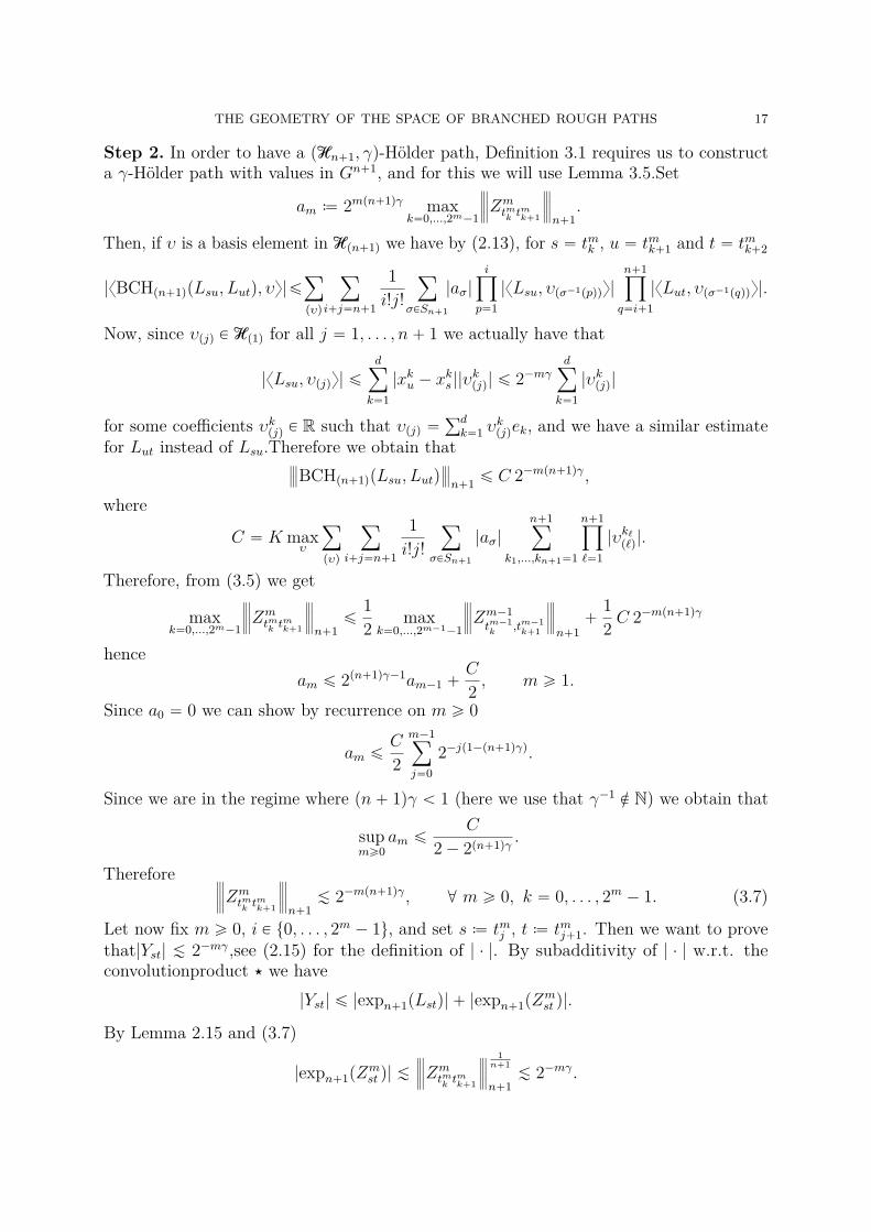
Step 2. In order to have a pHn`1, γq-Hölder path, Definition 3.1 requires us to constructa γ-Hölder path with values in Gn`1, and for this we will use Lemma 3.5.Set
am – 2mpn`1qγ maxk“0,...,2m´1
Zmtmktmk`1
n`1.
Then, if υ is a basis element in Hpn`1q we have by (2.13), for s “ tmk , u “ tmk`1 and t “ tmk`2
|xBCHpn`1qpLsu, Lutq, υy|ďÿ
pυq
ÿ
i`j“n`1
1i!j!
ÿ
σPSn`1
|aσ|iź
p“1|xLsu, υpσ´1ppqqy|
n`1ź
q“i`1|xLut, υpσ´1pqqqy|.
Now, since υpjq P Hp1q for all j “ 1, . . . , n` 1 we actually have that
|xLsu, υpjqy| ďdÿ
k“1|xku ´ x
ks ||υ
kpjq| ď 2´mγ
dÿ
k“1|υkpjq|
for some coefficients υkpjq P R such that υpjq “řdk“1 υ
kpjqek, and we have a similar estimate
for Lut instead of Lsu.Therefore we obtain that
BCHpn`1qpLsu, Lutq
n`1 ď C 2´mpn`1qγ,
where
C “ K maxυ
ÿ
pυq
ÿ
i`j“n`1
1i!j!
ÿ
σPSn`1
|aσ|n`1ÿ
k1,...,kn`1“1
n`1ź
`“1|υk`p`q|.
Therefore, from (3.5) we get
maxk“0,...,2m´1
Zmtmktmk`1
n`1ď
12 maxk“0,...,2m´1´1
Zm´1tm´1k
,tm´1k`1
n`1`
12 C 2´mpn`1qγ
henceam ď 2pn`1qγ´1am´1 `
C
2 , m ě 1.Since a0 “ 0 we can show by recurrence on m ě 0
am ďC
2
m´1ÿ
j“02´jp1´pn`1qγq.
Since we are in the regime where pn` 1qγ ă 1 (here we use that γ´1 R N) we obtain that
supmě0
am ďC
2´ 2pn`1qγ .
Therefore
Zmtmktmk`1
n`1À 2´mpn`1qγ, @ m ě 0, k “ 0, . . . , 2m ´ 1. (3.7)
Let now fix m ě 0, i P t0, . . . , 2m ´ 1u, and set s– tmj , t– tmj`1. Then we want to provethat|Yst| À 2´mγ,see (2.15) for the definition of | ¨ |. By subadditivity of | ¨ | w.r.t. theconvolutionproduct ‹ we have
|Yst| ď |expn`1pLstq| ` |expn`1pZmst q|.
By Lemma 2.15 and (3.7)
|expn`1pZmst q| À
Zmtmktmk`1
1n`1
n`1À 2´mγ.

18 N. TAPIA AND L. ZAMBOTTI
Moreover, using Lemma 2.15 again (first the upper bound, then the lower bound) and thefact that Xn : r0, 1s Ñ Gn is γ-Hölder by assumption,
|expn`1pLstq| ď Cn`1 supk“1,...,n`1
~pLstqk~1k“ Cn`1 sup
k“1,...,n~pLstqk~
1kď
ďCn`1
cn|expnpLstq| “
Cn`1
cn|Xst| “
Cn`1
cnρn
´
Xntmj,Xn
tmj`1
¯
À 2´mγ.
Therefore, the path Xn`1 : D Ñ Gn`1 defined by Xn`1tmj
– Y0,tmj satisfies
ρn`1
´
Xn`1tmj
,Xn`1tmj`1
¯
À 2´mγ,
thus by Lemma 3.5 we obtain a γ-Hölder path Xn`1 : r0, 1s Ñ Gn`1 extendingXn.
Remark 3.6. Our construction depends on a finite number of choices, namely we setZ01 “ 0 to start the recursion in (3.6), and this for each level; moreover in (3.6) we makethe choice Ztm2k,tm2k`1
“ Ztm2k`1,tm2k`2
. These choices are the same as in [30, Proof of Theorem1] and are indeed the most natural ones, but one could change them and thefinal outcomewould be different.
Remark 3.7. While in [30, Proof of Proposition 6] Lyons and Victoir use the axiomof choice, our proof is completely constructive. In particular, we use the explicit mapexpk`1 ˝ logk : GkpTnq Ñ Gk`1pTnq which plays the roleof the injection iGK,G : GK Ñ Gin [30, Proposition 6]. The fact that this map has goodcontinuity estimates is based onLemma 2.15.
Corollary 3.8. Given γ P s0, 1r with γ´1 R N and a collection of γ-Hölder paths xi : r0, 1s ÑR, i “ 1, . . . , d, there exists a γ-Hölder path X : r0, 1s Ñ GN such that xX, eiy “ xi ´ xi0,i “ 1, . . . , d. Then Xst – X´1
s ‹ Xtdefines a pH, γq-rough path over px1, . . . , xdq.
Proof. We start with the following observation: for n “ 1, the group G1 Ă H˚p1q is abelian,
and isomorphic to the additive group H˚p1q.Indeed, let X, Y P G1 and x P Hp1q. Then, as
∆x “ xb 1` 1b x by the grading, we have thatxX ‹ Y, xy “ xX, xy ` xY, xy,
that is, X ‹ Y “ X ` Y .Moreover, in H1 the product xy “ 0.Therefore, we may setxX1
t , eiy – xit ´ xi0 where te1, . . . , edu is a basis of Hp1q and this path is γ-Hölder withrespect to ρ1.By Theorem 3.4 there is a γ-Hölder path X2 : r0, 1s Ñ pG2, ρ2q extendingX1 so in particular xX2
t , eiy “ xit ´ xi0 also.Continuing in this way we obtain successiveγ-Hölder extensions X3, . . . ,XN and we set X – XN .
The following result has already been proved in the case where the underlying Hopfalgebra H is combinatorial by Curry, Ebrahimi-Fard, Manchon and Munthe-Kaas in [14,Theorem 4.3].We remark that their proof works without modifications in our context sowe have
Theorem 3.9. Let X : r0, 1s Ñ GN be a γ-Hölder path with X0 “ 1 and suppose thatγ´1 R
N. There exists a path X : r0, 1s Ñ G such that |xX´1s ‹ Xt, vy| À |t ´ s|γ|v| for all
homogeneous v P H and extending X, in the sense that Xˇ
ˇ
HN“ X.

THE GEOMETRY OF THE SPACE OF BRANCHED ROUGH PATHS 19
Remark 3.10. In view of Theorem 3.9 we can replace the truncated group in Definition 3.1by the full group of characters G.What this means is that γ-rough paths are uniquelydefined once we fix the first N levels and since H is locally finite, this amounts to a finitenumber of choices. This is of course a generalization of the extension theoremof [29], seealso [25, Theorem 7.3] for the branched case.
4. Applications
We now apply Theorem 3.4 to various kinds of Hopf algebras in order to link this resultwith the contexts already existing in the literature.
4.1. Geometric rough paths. In this setting we fix a finite alphabet A– t1, . . . , du.Asa vector space H – T pAq is the linear span of the free monoid MpAq generated byA. The product on H is the shuffle product : Hb H Ñ Hdefined recursively by1 v “ v1 “ v for all v P H, where 1 P MpAq is the unit for the monoid operation, and
pau bvq “ apu bvq ` bpau vq
for all u, v P H and a, b P A, where au and bv denote the product of the letters a, b withthe words u, v in MpAq.The coproduct ∆ : HÑ HbH is obtained by deconcatenation ofwords,
∆pa1 ¨ ¨ ¨ anq “ a1 ¨ ¨ ¨ an b 1` 1b a1 ¨ ¨ ¨ an `n´1ÿ
k“1a1 ¨ ¨ ¨ ak b ak`1 ¨ ¨ ¨ an.
It turns out that pH,, ∆q is a commutative unital Hopf algebra, and pH, ∆q is the cofreecoalgebra over the linear span of A.The antipode is the linear map S : HÑ H given by
Spa1 ¨ ¨ ¨ anq “ p´1qnan . . . a1.
Finally, we recall that H is graded by the length `pa1 ¨ ¨ ¨ anq “ n and it is also connected.Thehomogeneous components Hpnq are spanned by the sets ta1 ¨ ¨ ¨ an : ai P Au.Definition 3.1specializes in this case to geometric rough paths (GRP) as defined in [28] (see just belowfor the precise definition) and Theorem 3.4 coincides with [30, Theorem 6].
Definition 4.1. Let γ P s0, 1r and set N – tγ´1u. A geometric γ-rough path is a mapX : r0, 1s2 Ñ GN which satisfies Chen’s rule
Xst “ Xsu ‹Xut
for all s, u, t P r0, 1s and the analytic bound |xXst, vy| À |t´ s|γ`pvq for all v P HN .
Then Proposition 3.3 and the existence results Theorem 3.4-Corollary 3.8 are the contentof the paper [30] by Lyons and Victoir.

20 N. TAPIA AND L. ZAMBOTTI
4.2. Branched rough paths. Let Tbe the collection of all non-planar non-empty rootedtrees with nodes decorated by t1, . . . , du.Elements of T are written as 2-tuples τ “ pT, cqwhere T is a non-planar tree with node set NT and edge set ET , and c : NT Ñ t1, . . . , duis a function.Edges in ET are oriented away from the root, but this is not reflected in ourgraphical representation. Examples of elements of T include the following
i, ij,
ij k,
ijk l
m.
For τ P Twrite |τ | “ #NT for its number of nodes. Also, given an edge e “ px, yq P ET weset speq “ x and tpeq “ y.There is a natural partial order relation on NT where x ď y if andonly if there is a path in T from the root to y containing x.We denote by F the collectionof decorated rooted forests and we let H– HBCK denote the vector space spanned byF.There is a natural commutative and associative product on F, denoted by ¨ and given bythe disjoint union of forests, where the empty forest 1 acts as the unit.Then, H is the freecommutative algebra over T, with grading |τ1 ¨ ¨ ¨ τk| “ |τ1| ` ¨ ¨ ¨ ` |τk|.Given i P t1, . . . , duand a forest τ “ τ1 ¨ ¨ ¨ τk we denote by rτ1 ¨ ¨ ¨ τksi the tree obtained by grafting each of thetrees τ1, . . . , τk to a new root decorated by i, e.g.
r jsi “ ij, r j ksi “ i
j k.
The decorated Butcher–Connes–Kreimer coproduct [12, 25] is the unique algebra morphism∆: HÑ HbH such that
∆rτ si “ rτ si b 1` pidb r¨siq∆τ.
This coproduct admits a representation in terms of cuts.An admissible cut C of a treeT is a non-empty subset of ET such that any path from any vertex of the tree to theroot contains at most one edge from C; we denote by ApT q the set of all admissiblecuts of the tree T .Any admissible cut C containing k edges maps a tree T to a forestCpT q “ T1 ¨ ¨ ¨Tk`1 obtained by removing each of the edges in C.Observe that only oneof the remaining trees T1, . . . , Tk`1 contains the root of T , which we denote by RCpT q;the forest formed by the other k factors is denoted by PCpT q.This naturally induces amap on decorated trees by considering cuts of the underlying tree, and restriction of thedecoration map to each of the rooted subtrees T1, . . . , Tk`1.Then,
∆τ “ τ b 1` 1b τ `ÿ
CPApτq
PCpτq bRC
pτq. (4.1)
This, together with the counit map ε : FÑ R such that εpτq “ 1 if and only if τ “ 1 endowsFwith a connected graded commutative non-cocommutative bialgebra structure, hence aHopf algebra structure [31].As before we denote by H˚ the linear dual of Hwhich is analgebra via the convolution product xX ‹Y, τy “ xXbY,∆τy and we denote by G the set ofcharacters on H, that is, linear functionals X P H˚ such that xX, σ ¨ τy “ xX, σyxX, τy.Foreach n P N the finite-dimensional vector space Hn spanned by the set Fn of forests with atmost n nodes is a subcoalgebra of H, hence its dual is an algebra under the convolutionproduct, and we let Gn be the set of characters on Hn.We have already defined branchedrough paths in Definition 1.1.Proposition 3.3 yields the following characterization
Proposition 4.2. A path X : r0, 1s2 Ñ GN is a branched rough path if and only ifXt – X0t is γ-Hölder path with respect to thedistance ρN defined in (2.16).
THE GEOMETRY OF THE SPACE OF BRANCHED ROUGH PATHS 21
Directly applying Theorem 3.4 to the Butcher-Connes-Kreimer Hopf algebra H weobtain
Corollary 4.3. Given γ P s0, 1r with γ´1 R N and a family of γ-Hölder paths pxi : i “1, . . . , dq, there exists a branched rough path X above pxi : i “ 1, . . . , dq, i.e. X : r0, 1s2 ÑGN is such thatxXst, iy “ xit ´ x
is for all i “ 1, . . . , d.
Remark 4.4. Given the level of generality in which Theorem 3.4 is developed, our resultsalso apply to the case when H is a combinatorial Hopf algebra as defined in [14].Inparticular, we also have a construction theorem for planarly branched rough paths [14]which are characters over Munthe-Kaas and Wright’s Hopf algebra of Lie group integrators[32].
4.3. Anisotropic geometric rough paths. We now apply our results to another classof rough paths which we call anisotropic geometric rough paths (aGRPs for short).L.Gyurkó introduced a similar concept in [26], which he called Π-rough paths; unlike us, heuses a “primal” presentation, i.e. paths taking values in the tensor algebra T pRdq, andp-variation norms rather than Hölder norms. Geometric rough paths over a inhomogeneous(or anisotropic) set of paths can be traced back to Lyons’ original paper [29].As in thegeometric case, see Section 4.1, fix a finite alphabet A “ t1, . . . , du and denote by MpAqthe free monoid generated by A. We denote again by H– T pAq the shuffle Hopf algebraover the alphabet A.Let pγa : a P Aq be a sequence of real numbers such that 0 ă γa ă 1for all a, and let γ “ minaPA γa.For a word v “ a1 ¨ ¨ ¨ ak P MpAq of length k define
ωpvq– γa1 ` . . .` γak
and observe that ω is additive in the sense that ωpuvq “ ωpuq`ωpvq for each pair of wordsu, v P MpAq.The set
L – tv P MpAq : ωpvq ď 1uis finite; if N – tγ´1u then L Ă HN .In analogy with Lemma 2.5, the additivity of ω implies
Lemma 4.5. The subspace Ha Ă HN spanned by L is a subcoalgebra of pH, ∆, εq.
Consequently, we will consider the dual algebra pH˚a , ‹, εq. In this case, we define ga
to be the space of truncated infinitesimal characters on Ha, namelythe linear functionalsα P H˚
a such thatxα, x yy “ xα, xyxε, yy ` xε, xyxα, yy
for all x, y P Ha such that x y P Ha,and let Ga – tX “ expNpαq|Ha: α P gau.As before,
there is a canonical injection H˚a ãÑ H˚ so we suppose that xX, vy “ 0 for all X P H˚ and
v R L.For each λ ą 0 there is a unique coalgebra automorphism Ωλ : HÑ H such thatΩλa “ λγaγa for all a P A. We also define ¨ : Ga Ñ R,
X– maxvPL
|xX, vy|γωpvq. (4.2)
As at the end of Section 2, pΩλqλą0 is a one-parameter family of Lie-algebra automorphismsof ga andΩλX “ λX for all λ ą 0 and X P Ga, namely ¨ is a homogeneous norm onGa. However, unlike ~¨~ this norm is not subadditive and it therefore does not define adistance on Ga.

22 N. TAPIA AND L. ZAMBOTTI
4.3.1. Signatures. In order to construct an appropriate metric on Ga we consider signaturesof smooth paths. We observe that A Ă L.Let x “ pxa : a P Aq be a collection of (piecewise)smooth paths, and define a map Spxq : r0, 1s2 Ñ H˚ by
xSpxqst, vy–
ż t
s
dxvkskż sk
s
dxvk´1sk´1
¨ ¨ ¨
ż s2
s
dxv1s1 .
In his seminal work [11], K. T. Chen showed that Spxq is a character of pT pAq,q; inparticular, Spxqst|Ha
P Ga.Consider the metric dapX, Y q “ř
aPA |xX ´ Y, ay|γγa on H˚p1q,
where we recall that Hp1q is the vector space spanned by A.The anisotropic length ofa smooth curve θ : r0, 1s Ñ H˚
1 is defined to be its length with respect to this metricand will be denoted by Lapθq.Observe that since dapΩλX,ΩλY q “ λdapX, Y q we havethat LapΩλθq “ λLapθq.We now define a homogeneous norm (see the end of Section 2)| ¨ |CC : Ga Ñ R`, called the anisotropic Carnot–Carathéodory norm, by setting
|X|CC – inftLapxq : xa P C8, Spxq01 “ Xu.
Since curve length is invariant under reparametrization in any metric space we obtain, asin [23, Section 7.5.4]:
Proposition 4.6. The infimum defining the anisotropic Carnot–Carathéodory norm isfinite and attained at some minimizing path x.
Proposition 4.7. The anisotropic Carnot–Carathéodory norm is homogeneous, that is,|ΩλX|CC “ λ|X|CC.
Proof. Let x be the curve such that |X|CC “ Lapxq. For any λ ą 0 and word v P L wehave
xSpΩλxq01, vy “ λωpvqγxSpxq01, vy “ xΩλSpxq01, vy “ xΩλX, vy,
thus |ΩλX|CC ď LapΩλxq “ λLapxq “ λ|X|CC.The reverse inequality is obtained by notingthat X “ pΩλ´1 ˝ ΩλqX.
The anisotropic Carnot–Carathéodory norm can also be seen to satisfy |X|CC “ |X´1|CC
and|X ‹ Y |CC ď |X|CC ` |Y |CC for all X, Y P Ga, see e.g. the proof of [23, Proposition7.40];hence it induces a left-invariant metric ρapX, Y q – |X´1 ‹ Y |CC on Ga.Moreover,arguingas in the proof of [23, Theorem 7.44] we see that there exist positive constants c, Csuch that
c|X|CC ď X ď C|X|CC, @ X P Ga. (4.3)
Definition 4.8. An anisotropic geometric γ-rough path, with γ “ pγa, a P Aq, is a mapX : r0, 1s2 Ñ Ga which satisfies
(1) the Chen rule Xsu ‹Xut “ Xst for all ps, u, tq P r0, 1s3,(2) the bound |xXst, vy| À |t´ s|
ωpvq for all v P L.
Proposition 4.9. Anisotropic geometric γ-rough paths are in one-to-one correspondencewith γ-Hölder paths X : r0, 1s Ñ pGa, ρaq with X0 “ 1.
Proof. Let X be an anisotropic geometric γ-rough path and v a word. By definition wehave that |xXst, vy| À |t´ s|
ωpvq, hence Xst À |t´ s|γ.The equivalence between ¨ and

THE GEOMETRY OF THE SPACE OF BRANCHED ROUGH PATHS 23
| ¨ |CC of (4.3) implies that ρapXs,Xtq “ |Xst|CC À |t´ s|γ , hence t ÞÑ Xt is γ-Hölder with
respect to ρa.The other direction follows in a similar manner.
Theorem 3.4 also applies to this situation, and we obtain the following
Corollary 4.10. Let pγa : a P Aq be real numbers in s0, 1r such that 1 Rř
aPA γaN.Letpxa : a P Aq be a collection of real-valued paths such that xa is γa-Hölder. Thenthere existsan anisotropic geometric γ-rough path X such that xXst, ay “ xat ´ x
as for all a P A.
Proof. We start by constructing the homogeneous geometric rough path X given by theγ-Hölder path X : r0, 1s Ñ GN ofCorollary 3.8. Then we restrict X to Ha Ă HN andwe show that on this space it satisfies the stronger bound |xXst, vy| À |t ´ s|ωpvq for allv P L.Recalling the proof of Theorem Theorem 3.4, we consider v P Hn X Ha, and weproceed by recurrence on n.For n “ 0 there is nothing to prove. Suppose we have provedthe result for n and let v P Hn`1 XHa. In this case
xXn`1st , vy “ xexpn`1pLst ` Zstq, vy “
n`1ÿ
i“0
1i!xpLstq
i‹‹ pε` Zstq, vy
“
n`1ÿ
i“0
1i!xpLstq
i‹, vy ` xZst, vy “ xXnst, vy `
1pn` 1q!xpLstq
pn`1q‹, vy ` xZst, vy.
We want to prove now thatˇ
ˇ
ˇxXn`1
tmktmk`1, vy
ˇ
ˇ
ˇÀ 2´mωpvq, @m ě 0, k “ 0, . . . , 2m ´ 1. (4.4)
For m ě 0 setbm – 2mωpvq max
k“0,...,2m´1
ˇ
ˇ
ˇxZm
tmktmk`1, vy
ˇ
ˇ
ˇ.
Then, for s “ tmk , u “ tmk`1 and t “ tmk`2 and v “ v1 ¨ ¨ ¨ vn`1
|xBCHpn`1qpLsu, Lutq, vy| ďÿ
i`j“n`1
1i!j!
ÿ
σPSn`1
|aσ|iź
p“1|xLsu, vσ´1ppqy|
n`1ź
q“i`1|xLut, vσ´1pqqy|.
Now, since vj P Hp1q for all j “ 1, . . . , n ` 1 we actually have that by the assumptionxa P Cγa
|xLsu, ay| “ |xau ´ x
as | À 2´mγa
and we have a similar estimate for Lut instead of Lsu.Therefore we obtain thatˇ
ˇxBCHpn`1qpLsu, Lutq, vyˇ
ˇ À 2´mωpvq.
Therefore, from (3.5) we get
bm ď 2mpωpvq´1qbm´1 ` C, m ě 1,
hence since b0 “ 0 we can show by recurrence on m ě 0
bm ď Cm´1ÿ
j“02´jp1´ωpvqq.
24 N. TAPIA AND L. ZAMBOTTI
Since we are in the regime where ωpvq ă 1 (here we use that 1 Rř
aPA γaN) we obtain that
supmě0
bm ďC
1´ 2ωpvq´1 .
Thereforeˇ
ˇ
ˇxZm
tmktmk`1, vy
ˇ
ˇ
ˇÀ 2´mωpvq, m ě 0, k “ 0, . . . , 2m ´ 1.
Analogously, since Lst P g, arguing as in (2.14) we have
xpLstqpn`1q‹, vy “
n`1ź
i“1xLst, viy “
n`1ź
i“1pxvit ´ x
vis q ùñ
ˇ
ˇxpLstqpn`1q‹, vy
ˇ
ˇ À 2´mωpvq
and (4.4) is proved. This implies that Xn`1tmktmk`1 À 2´mγand by equivalence of homogeneous
norms (4.3) we obtainρa
´
Xn`1tmk,Xn`1
tmk`1
¯
À 2´mγ.
Then we can use Lemma 3.5 and obtain that the path Xn`1 constructedin the proof ofTheorem 3.4 is in fact γ-Hölder path withvalues in Ga.
5. The Hairer-Kelly construction
In this section we develop further results specifically for branched rough paths asintroduced in Section 4.2 by using our general results from Section 3.We analyze indetail the Hairer-Kelly map introduced in [28], which plays a very important role in ourconstruction, and we use it to prove Theorem 1.2 and Corollary 1.3.
5.1. The Hairer–Kelly map. Recall that Tdenotes the set of all decorated rooted trees,F denotes the collection of all decorated rooted forests, and HBCK is the Butcher–Connes–Kreimer Hopf algebra. As in Section 4.2, ∆ denotes the Connes–Kreimer coproduct onHBCK.For each n P N, n ě 1, we denote by Tn the set of (non-empty) trees with at mostn vertices.Recall also from Section 4.1 that given an alphabet A we denote by T pAq theshuffle Hopf algebra generated by A, and that ∆ denotes the deconcatenation coproducton it. We fix N P N and we consider the shuffle Hopf algebras T pTq and T pTNq,namelywe choose as letters of our alphabet the (non-empty) decorated rooted trees (respectivelyrooted trees with with at most N vertices).Note that we can identify every non-empty treeτ P Twith theword in T pTq composed by the single letter τ .We also remark that, in orderto avoid confusion with the forest product on HBCK we denote the concatenation of lettersin T pTq by a tensor symbol.We note that T pTq and T pTNq admit two different naturalgradings, both of which make them locally finite graded Hopf-algebras. One grading,asin Section 4.1, is given by the number of letters (trees) of each word, namely the degreeof v “ τ1 b ¨ ¨ ¨ b τk is k. Theother grading is given by the sum of the number of nodesof each letter (tree), namely the degree of v “ τ1 b ¨ ¨ ¨ b τk is|τ1| ` ¨ ¨ ¨ ` |τk|, where werecall that forests and trees are graded in HBCK by the number of nodes, with the notation|τ | “ #Nτ . We remark the latter grading is always greater or equal to the former. As anexample, take v “ i b j
k; then, as a word v has length 2 but the total number of nodes is3.We recall the following result from [28, Lemma 4.9].

THE GEOMETRY OF THE SPACE OF BRANCHED ROUGH PATHS 25
Lemma 5.1. We grade T pTq according to the number of nodes. Then there exists a gradedmorphism of Hopf algebras ψ : HBCK Ñ T pTq satisfying ψpτq “ τ `ψn´1pτq for all τ P Tn,where ψn´1 denotes the projection of ψ onto T pTn´1q.
We call ψ the Hairer-Kelly map. Since ψ is graded, for any forest τ P Fthe image ψpτq isa sum of words of the formτ1b¨ ¨ ¨b τk where all terms satisfy |τ1|` ¨ ¨ ¨` |τk| “ |τ |.Observethat since ψ is a Hopf algebra morphism, in particular a coalgebra morphism, then
pψ b ψq∆1τ “ ∆1ψpτq “ ∆1ψn´1pτq, τ P Tn,
since trees are primitive elements in T pTq, being single-letter words.From the proof of[28, Lemma 4.9] we are able to see that in fact ψn´1 is given by the recursion ψn´1 “
mbpψ b idq∆1 on the linear span of Tn, see also [3, Definition 1, section 6].
Example 5.2. Here are some examples of the action of ψ on some trees:
ψp iq “ i, ψp a bq “ ψp aq ψp bq “ a b b ` b b a, ψ`
ab˘
“ ab ` b b a
ψ´
acdb
¯
“acdb ` b b
acd` d b a
c d ` cd b a
b ` d b c b ab ` d b b b a
c ` b b d b ac
` cd b b b a ` b b c
d b a ` d b c b b b a ` d b b b c b d
` b b d b c b a.
5.2. A special class of anisotropic geometric rough paths. We have already dis-cussed anisotropic geometric rough paths (aGRPs) in Section 4.3. For the Hairer-Kellyconstructionwe need a very particular subclass of aGRPs, where the base paths pxaqaPAare such that each xa isγa-Hölder and there exists γ P s0, 1r and pkaqaPA Ă N such thatγa “ kaγ; therefore the Hölder exponents are all integer multiples of a fixed exponentγ.We may of course apply the extension result of Corollary 4.10, but it turns out that inthis setting wecan avoid using the Carnot-Carathéodory distance and rather use a moreexplicit metric, which is a simplegeneralization of the homogeneous case (2.16).We havealready seen that the space H– T pTNq can be graded in two ways. We can even definea bigrading on thisspace: for 1 ď n ď N andn ď j ď nN , we define the space Hpn,jq asthe linear span of the words τ1 b ¨ ¨ ¨ b τn P T pTNq such that|τ1| ` ¨ ¨ ¨ ` |τn| “ j. Then, inanalogy with (2.2), we have
: Hpn,jq bHpm,hq Ñ Hpn`m,j`hq, ∆ : Hpn,jq Ñà
p“0,...,n, q“1,...,j´1Hpp,qq bHpn´p,j´qq.
Then, recalling that H0 “ R1, we set
HN,N – H0 ‘Nà
n“1
Nà
j“n
Hpn,jq.
In other words, HN,N is the linear span of all words τ1 b ¨ ¨ ¨ b τn with n ď N and|τ1| ` ¨ ¨ ¨ ` |τn| ď N .Therefore, analogously to (2.3) and (2.5), we have decompositions
HN,N Q x “ x0 `
Nÿ
n“1
Nÿ
j“n
xn,j, H˚N,N Q α “ αp0q `
Nÿ
n“1
Nÿ
j“n
αpn,jq, αpn,jqpxq “ αpxn,jq.

26 N. TAPIA AND L. ZAMBOTTI
We define now gN,N as the space of truncated characters on HN,N , namely of all linearα : HN,N Ñ R such that
xα, x yy “ xα, xyxε, yy ` xε, xyxα, yy
for all x, y P HN,N such that x y P HN,N . Moreover we define GN,N – expNpgN,Nq ĂH˚N .Then we set in analogy with (2.17) for X P GN,N
|X| – N maxn“1,...,N
ˆ
maxj“n,...,N
`
j!
Xpn,jq
˘1j` max
j“n,...,N
´
j!
`
X´1˘
pn,jq
¯1j˙
, (5.1)
and we can see that
Lemma 5.3. The map GN,N ˆGN,N Q pX, Y q ÞÑ ρN,NpX, Y q – |X´1 ‹ Y | P R defines adistance on GN,N .
Proof. We only have to check the triangular inequality, which is equivalent to the sub-additivity property |X ‹ Y | ď |X| ` |Y | forall X, Y P GN,N . Arguing as in the proof ofProposition 2.14
pX ‹ Y qpn,jq
ď
nÿ
m“0
j´1ÿ
i“1
Xpm,jq
Ypn´m,j´iq
ď N1j!
1N2
jÿ
i“0
ˆ
j
i
˙
|X|i|Y |j´i “1N
1j!p|X| ` |Y |q
j
whence the result.
Let γ P s0, 1r and N – tγ´1u.In accordance with Definition 4.8, an anisotropic geometricγ-rough path in this setting is a map X : r0, 1s2 Ñ GN,N which satisfies
(1) the Chen rule Xsu ‹Xut “ Xst for all ps, u, tq P r0, 1s3,(2) |xXst, vy| À |t´ s|
jγ for all v P Hpn,jq with 1 ď n ď N and j ď N .
Then, arguing as in Proposition 3.3, it is easy to show that X : r0, 1s Ñ GN,N is γ-Hölderwith respect to the metric ρN,N if and only ifX : r0, 1s2 Ñ GN,N , defined asXst – X´1
s ‹Xt,isan anisotropic geometric γ-rough path with γv “ jγ for v “ τ1 b ¨ ¨ ¨ b τn with n ď N and|τ1| ` ¨ ¨ ¨ ` |τn| “ j ď N .The next result is the analog of Corollary 4.10 in this setting.The proof is the same, with one exception: we can use the explicit norm(5.1) rather thanthe Carnot-Carathéodory norm | ¨ |CC and we do not need the equivalence of norms result(4.3).
Proposition 5.4. Given γ P s0, 1r with γ´1 R N and a collection of paths xτ : r0, 1s Ñ R,τ P TN , such that xτ P Cγ|τ |, there exists a γ-Hölder path X : r0, 1s Ñ GN,N such thatxX, τy “ xτ for all τ P TN .
Corollary 5.5. In the setting of Proposition 5.4, let pgτ : τ P TNq bea collection offunctions with gτ P Cγ|τ |. Set xτt “ xτt ` gτt and denote by gX the anisotropic geometricγ-rough path constructed in Proposition 5.4 above the path
xt “ÿ
τPTN
xτt τ P Hp1q, t P r0, 1s.

THE GEOMETRY OF THE SPACE OF BRANCHED ROUGH PATHS 27
Then, for any two such functions g and g1 we have that g1pgXq “ pg ` g1qX.
Proof. Let g, g1 be two collections of functions as in the statement of the theorem. Wehave the identity
xrg1pgXqst, τy “ xpgXqt, τy ` pg1qτt “ xτt ` g
τt ` pg
1qτt “ xrpg
1` gqXst, τy.
Since both g1pgXq and pg1 ` gqX are constructed iteratively by adding at each step afunction Z satisfying (3.6) on the dyadics, if we let Ln and Ln denote the logarithmscorresponding to g1pgXq and pg1 ` gqX, Lemma 2.13 and the previous identity imply that
BCHn`1pLnsu, L
nutq “ BCHn`1pL
nsu, L
nutq
and so g1pgXq “ pg1 ` gqX.
5.3. Branched rough paths are anisotropic geometric rough paths. The nexttheorem is almost the same statement as Theorem 4.10 in [28], the only difference beingthatwe construct an anisotropic geometric rough path X while Hairer-Kelly need only that Xis geometric in the usual sense (see also [28, Remark 4.14].
Theorem 5.6. Let γ P s0, 1r with γ´1 R N, andlet X be a branched γ-rough path. Thereexists an anisotropic geometric rough path X : r0, 1s2 Ñ GN,N with exponents γ “ pγτ “γ|τ |, τ P TNq, and such that
xX, τy “ xX, ψpτqy, @ τ P FN .
Proof. We construct X iteratively as follows.Let Xp1q be the anisotropic geometric roughpath indexed by T1 “ t 1, . . . , du over the paths pxit – xXt, iy : i “ 1, . . . , dq withexponents pγ i “ γq given by Proposition 5.4 (alternatively we could use have usedTheorem 3.4 since all the exponents are equal). This will give us an anisotropic rough pathpath X : r0, 1s2 Ñ GapT1q with exponents pγτ “ γ, τ P T1q.Suppose we have constructedanisotropic geometric rough paths Xpkq : r0, 1s2 Ñ GapTkq over the paths pxτ : τ P Tkq
such that xτt ´ xτs “ xXst, τy ´ xXpk´1qst , ψk´1pτqy for k “ 1, . . . , n.This is true for n “ 1
by the previous paragraph, since ψp iq “ i for all i “ 1, . . . , d.If we let F τst “ xXst, τy and
Gτst “ xX
pnqst , ψnpτqy for τ P Tn`1 we have, by Chen’s rule, that
δF τsut “ xXsu bXut,∆1τy “ xXpnq
su ˝ ψ b Xpnqut ˝ ψ,∆1τy.
Since ψ is in particular a coalgebra morphism between pH,∆q and pT pTNq, ∆q we obtainthe identity δF τ
sut “ xXpnqsu b X
pnqut , ∆1ψpτqy, which then, by Lemma 5.1 becomes
δF τsut “ xX
pnqsu b X
pnqut , ∆1ψnpτqy “ δGτ
sut. (5.2)since every τ P T is primitive in pT pTNq, ∆q being a single-letter word.The finite incrementoperator δ has the following property: if J : r0, 1s2 Ñ R is such that δJ “ 0 then thereexists f : r0, 1s Ñ R such that Jst “ ft´ fs, and the function f is unique up to an additiveconstant shift, see also [25, formula (5)].Thus, by this fundamental property, for eachτ P Tn`1 there exists a function xτ : r0, 1s Ñ R such that xτt ´ xτs “ F τ
st ´Gτst and then
|xτt ´ xτs | ď |xXst, τy| ` |xX
pnqst , ψnpτqy| À |t´ s|
γ|τ |

28 N. TAPIA AND L. ZAMBOTTI
since ψnpτq preserves the number of nodes by Lemma 5.1.Repeatedly using Proposition 5.4we obtain an anisotropic geometric rough path Xpn`1q : r0, 1s Ñ GapTn`1q over pxτ : τ PTn`1q whose restriction to T pTnq coincides with Xpnq.Finally notice that if τ P Tn`1 is atree then
xXpn`1qst , ψpτqy “ xX
p|τ |qst , τy ` xX
p|τ |qst , ψ|τ |´1pτqy
“ xτt ´ xτs ` xXst, τy ´ px
τt ´ x
τsq “ xXst, τy
and the corresponding identity for arbitrary forests follows by multiplicativity.The anisotropicgeometric rough path sought for is X “ XpNq.
We note that our proof is shorter and simpler than that of [28, Theorem 4.10], so wewill now dedicate a few paragraphs to highlight the differences between our approach andthat of Hairer and Kelly.They define first
X1t “ expN
˜
ÿ
aPA
xat a
¸
P GNpT1q
then they note that this is not γ-Hölder with values in GNpT1q, but it is γ-Hölder withvaluesinGNpT1qK1, whereK1 – expNpW2`¨ ¨ ¨`WNq, see (2.7). By the Lyons-Victoir extensiontheorem there exists a γ-Hölder path X1
t Ñ GNpT1qsuch that πGN pT1qÑGN pT1qK1pX1q “ X1.Then, in order to add a new tree τ with |τ | “ 2, they define
pδXτqst “ xXst, τy ´ xX
p1qst , ψ1pτqy
and this defines the new function t ÞÑ xXt, τy. Then theydefine
X2t “ expN
˜
ÿ
aPA
xat a `ÿ
|τ |“2xXt, τy τ
¸
P GNpT2q
and again they note that this path is not γ-Hölder with values in GNpT2q, but it is withvalues in GNpT2qK2, where K2 – expNpW3 ` ¨ ¨ ¨ `WNq, and again the Lyons-Victoirextension theorem yieldsa γ-Hölder path X2
t Ñ GNpT2qsuch that πGN pT2qÑGN pT2qK2pX2q “
X2. Finally they construct recursively in this way Xk and Xk for all k ď N .At this point wesee the difference with our approach. We do not define X2
t nor Xk butrather we constructX step by step, namely on all GkpTnq with 1 ď k, n ď N ,first by recursion on k for fixed nand then by recursion on n;at each step we enforce the Hölder continuity on GkpTnq andthecompatibility with the previous levels. This is done using the Lyons-Victoir technique,butin a very explicit and constructive way, in particular without ever using the axiom ofchoice,since we have the explicit map expk`1 ˝ logk : GkpTnq Ñ Gk`1pTnq which playstherole of the injection iGK,G : GK Ñ G in [30, Proposition 6].
6. An action on branched rough paths
In this section we prove Theorem 1.2.Given γ P s0, 1r, let N “ tγ´1u and denote by Cγ
the set of collections of functions pgτ qτPTN such that gτ P Cγ|τ | and gτ0 “ 0 for all τ P TN .Itis easy to see that Cγ is a group under pointwise addition in t, that is,
pg ` hqτ – gτ ` hτ .

THE GEOMETRY OF THE SPACE OF BRANCHED ROUGH PATHS 29
As a consequence of Proposition 5.4, pg, Xq ÞÑ gX is an action of Cγ on the space ofanisotropic geometric rough paths.We use the Hairer-Kelly map ψ of Lemma 5.1 to inducean action of Cγ on branched rough paths.Given a branched rough path X and g P Cγ welet gX be the branched rough path defined by
xgXst, τy “ xgXst, ψpτqy,
where X is the anisotropic geometric rough path given by Theorem 5.6.As a simpleconsequence of Proposition 5.4 we obtain
Proposition 6.1. Let X P BRPγ.
(1) We have g1pgXq “ pg1 ` gqX for all g, g1 P Cγ.(2) If pgτ qτPTN P Cγ is such that there exists a unique τ P TNwith gτ ı 0, then
xpgXqst, τy “ xXst, τy ` gτt ´ g
τs
and xgX, σy “ xX, σy for all σ P T not containing τ as a subtree.
Proof. The first claim follows from point (1) in Proposition 5.4. In order to prove thesecond claim, letg “ pgτ qτPTN P Cγ be such that there exists a unique τ P TNwith gτ ı 0.Then by the property of g we have
xgX, τy “ xgX, ψpτqy “ xgX, τ ` ψ|τ |´1pτqy
“ xX, τy ` δgτ ` xgX, ψ|τ |´1pτqy
where δgτst – gτt´gτs .By Lemma 5.1 the tree τ does not appear as a factor in any of the tensor
products appearing in ψ|τ |´1pτq, hence one can recursively show that xgX, ψ|τ |´1pτqy “
xX, ψ|τ |´1pτqy so that the above expression becomes
xgX, τy “ xX, τ ` ψ|τ |´1pτqy ` δgτ
“ xX, τy ` δgτ .
For the last assertion, it is enough to note that σ P T contains τ P T if and only if τappears in the expression for ψpσq; this can be expressed more precisely by saying thatσ R T pTNztτuq.But if σ P T pTNztτuq, then xgX, ψpτqy “ xX,ψpτqy.
Proposition 6.2. The action of Cγ on branched γ-rough paths is transitive: for everypair of branched γ-rough paths X and X 1 there exists g P Cγ such that gX “ X 1.
Proof. We define g P Cγ inductively by imposing the desired identity.For trees τ P T1 “
t 1, . . . , du we set gτt “ xX 10t, τy ´ xX0t, τy P C
γ so that
xgX, τy “ xgX, ψpτqy “ xgX, τy “ xX, τy ` δgτ “ xX 1, τy
where δgτst – gτt ´ gτs . Suppose we have already defined gτ for all τ P Tn for some n ě 1,
satisfying the constraints in the definition of Cγ.For a tree τ with |τ | “ n` 1 we define
F τst “ xX
1st, τy ´ xXst, τy ´ xgXst, ψnpτqy.

30 N. TAPIA AND L. ZAMBOTTI
ThenδF τ
sut “ xX1su bX
1ut,∆1τy ´ xgXsu b gXut, ∆1ψnpτqy
“ xX 1su bX
1ut,∆1τy ´ xgXsu b gXut, ∆1ψpτqy
“ xX 1su bX
1ut,∆1τy ´ xgXsu ˝ ψ b gXut ˝ ψ,∆1τy
“ xX 1su bX
1ut,∆1τy ´ xgXsu b gXut,∆1τy “ 0
by the induction hypothesis. Hence there is gτ : r0, 1s Ñ R such that gτ0 “ 0 andgτt ´ g
τs “ xX
1st, τy ´ xXst, τy ´ xgXst, ψnpτqy (6.1)
whence g P Cγ|τ |; by constructionxgX, τy “ xgX, ψpτqy “ xgX, τy ` xgX, ψnpτqy
“ xX, τy ` δgτ ` xgX, ψnpτqy “ xX1, τy,
where δgτst “ gτt ´ gτs . This concludes the proof.
Proposition 6.3. The action of Cγ on branched γ-rough paths is free, namely if gX “ g1Xthen g “ g1.
Proof. This follows from the fact that by (6.1) the function gτ is defined up to a constantshift. Therefore, the condition gτ0 “ 0 determines gτ uniquely.
Together, Proposition 6.1, Proposition 6.2 and Proposition 6.3 imply Theorem 1.2.
6.1. The BCFP renormalisation. In [4] a different kind of modification is proposed.There,a new decoration 0 is considered so rough paths –branched and geometric– are over pathstaking values in Rd`1.Recall that since branched rough paths are seen as Hölder pathstaking values in the character group of the Butcher-Connes-Kreimer Hopf algebra, we maythink of them as an infinite forest series of the form
Xst “ÿ
τPF
xXst, τyτ (6.2)
where we regard τ as a linear functional on H, such that xτ, σy “ 1 if σ “ τ and zeroelse.The aforementioned modification procedure then acts as a translation of the series(6.2).Specifically, for each collection v “ pv0, . . . , vdq : TÑ Rd`1 an operator Mv : H˚ Ñ
H˚ is defined, such that for a γ-branched rough path, pMvXqst – MvpXstq is a γN -branched rough path.In the particular case where vj “ 0 except for v0, the action of thisoperator can be described in terms of an extraction/contraction map1 Ψ: HÑ HbH.Thismap acts on a tree τ by extracting subforests and placing them in the left factor; the rightfactor is obtained by contracting the extracted forest and decorating the resulting nodewith 0.As an example, consider
Ψpij kq “ 1b
ij k ` i b 0
j k ` j b i0 k ` k b i
j 0 `ij b 0
k ` ik b 0
j
` i j b 00 k ` i k b 0
j 0 ` j k b i0 0 `
ijk b 0
0 ` ik j b 0
0 `ij k b 0.
1In [4] this map is named δ but we choose to call it Ψ in order to avoid confusion with the operatordefined here.

THE GEOMETRY OF THE SPACE OF BRANCHED ROUGH PATHS 31
Extending v “ v0 : TÑ R to all of H˚ as an algebra morphism it is shown thatxpMvXqst, τy “ xXst, pv b idqΨpτqy. (6.3)
Furthermore, in this case MvX is a γ-branched rough path if coefficients corresponding totrees with decoration zero are required to satisfy the stronger analytical condition
sup0ďs,tď1
|xXst, τy|
|t´ s|p1´γq|τ |0`γ|τ |ă 8, (6.4)
where |τ |0 counts the times the decoration 0 appears in τ .Essentially, this condition imposesthat the components corresponding to the zero decoration be Lipschitz on the diagonals “ t.We now show how this setting can be recovered from the results of Section 6.LetX be a γ-branched rough path on Rd`1 satisfying (6.4).Since MvX is again a γ-branchedrough path, by Proposition 6.2 there exists a collection of functions g P Cγ such thatgX “MvX.Moreover, this collection is the unique one satisfying
gτt ´ gτs “ xXst, pv b idqΨpτqy ´ xXst, τy ´ xgXst, ψ|τ |´1pτqy (6.5)
for all τ P TpRd`1q where we have used (6.3) in order to express MvX in terms ofΨ.Theorem 28 in [4] ensures that the first term on the right-hand side is in Cγ|τ |
2 hence g isactually in Cγ|τ | as required.The approach of [4] is based on pre-Lie morphisms and cruciallyon a cointeraction property, which has been explored by [7], see in particular [4, Lemma 18].The cointeraction property can be used for time-independent modifications, indeed notethat the functional v in [4] is always constant.Let us see why this is the case. The approachof [4] is based on a cointeractionproperty studied by [6, 7, 21] between the Butcher-Connes-Kreimer coproduct and anotherextraction-contraction coproduct δ : HÑ HbH. Theformula is the following
pidb∆qδ “M1,3pδ b δq∆.Let us consider now a character v P H˚.If we multiply both sides by pv b idb idq and setM˚
v “ pv b idqδ : HÑ H as in [4, Proposition 17], then we obtain∆M˚
v “ pM˚v bM
˚v q∆,
namely M˚v is a coalgebra morphism on H. Then one can define a modified rough path
asvX –MvX “ X ˝M˚v . The crucial Chen property is still satisfied since
pvXqst “ pv bXstqδ “ pv bXsu bXutqpidb∆qδ“ pv bXsu bXutqM1,3pδ b δq∆“ ppv bXsuq b pv bXutqqpδ b δq∆“ ppvXqsu b pvXqutq∆
However this does not work if v : r0, 1s2 Ñ H˚ is a time-dependent character. Indeed inthis casewe set pvXqst – pvst b idqδ and we obtain
pvXqst “ pvst bXstqδ “ pvst bXsu bXutqpidb∆qδ“ pvst bXsu bXutqM1,3pδ b δq∆“ ppvst bXsuq b pvst bXutqqpδ b δq∆
but we can not conclude that this is equal to ppvXqsu b pvXqutq∆. Our construction, asexplained afterformula (1.8), is not purely algebraic but is based on a (non-canonical)choice of generalized Young integralswith respect to the rough path X.Moreover our

32 N. TAPIA AND L. ZAMBOTTI
transformation group, infinite-dimensional, is much larger than that finite-dimensionalgroup studiedin [4].
7. Perspectives
In this paper we have shown that the space of branched γ-rough paths is aprincipalhomogeneous space with respect to the linear group Cγ. This is related to theanalyticalproperties of the operator δ defined in (1.2), which is invertible under theconditions of Gubinelli’s Sewing Lemma, but not in general, and in particular not in thecontextof the Chen relation on trees with low degree.It would be now interesting to seehow this action can be translated on the level of controlled paths [24]. The space of pathscontrolled by a rough path X P BRPγ should be interpreted as thetangent space toBRPγ at X, and the action on rough paths should induce an action on controlled paths.In particular it should be possible to write an action on solutions to rough differentialequations.The proof of Proposition 6.2, and in particular (6.1), gives a recursive way ofcomputing the unique g P Cγ translating a given branched γ-rough path into another.Aninteresting feature of the BCFP scheme is that is given in terms of a coaction so explicitcalculations are somewhat easier in this more restricted case as one can compute gτ foreach tree τ P TN directly by extracting and contracting subforests of τ without doing anyrecursions (see (6.5).)However, we do not have a computational rule for an importantcase: suppose that X is branched rough path lift of a stochastic process with a.s. Cγ´
trajectories; it would be nice to have a way of finding g P Cγ such that gX is centeredwith respect to the underlying distribution of the process, provided this is possible.Eventhis last problem, namely giving precise conditions under which this centering is possibleis interesting in itself.This should be related to the notion of Wick polynomials anddeformations of products as considered in [18].More generally, in the physics literaturethere are various renormalisation procedures which allow to obtain convergent iteratedintegrals from divergent ones by subtracting suitable “counterterms”. In the context ofrough paths, implementing one of the most accepted such procedures due toBogoliubov–Parasiuk–Hepp–Zimmermman (BPHZ) has been carried out by J.Unterberger in [35, 36] by means of the Fourier normal ordering algorithm and using atechnique relating the trees in the Butcher–Connes–Kreimer Hopf algebra to certainFeynman diagrams.In our context, this could provide a canonical choice for g P Cγ
implementing the BPHZ renormalization procedure in a way analogous to what is done in[6] for Regularity Structures.
References[1] G. Ben Arous, “Flots et séries de Taylor stochastiques,”Probab. Theory RelatedFields 81 no. 1,
(1989) 29–77.[2] H. Boedihardjo and I. Chevyrev, “An isomorphism between branched and geometricrough paths,”
arXiv:1712.01965 [math.PR].[3] Y. Bruned, I. Chevyrev, and P. K. Friz, “Examples of renormalized SDEs,” inStochastic partial
differential equations and related fields, vol. 229of Springer Proc. Math. Stat., pp. 303–317.Springer,Cham, 2018.
[4] Y. Bruned, I. Chevyrev, P. K. Friz, and R. Preiß, “A Rough PathPerspective on Renormalization,”to appear in Journal ofFunctional Analysis (2019) ,arXiv:1701.01152[math.PR].
THE GEOMETRY OF THE SPACE OF BRANCHED ROUGH PATHS 33
[5] Y. Bruned, C. Curry, and K. Ebrahimi-Fard, “Quasi-shuffle algebras andrenormalisation of roughdifferential equations,”arXiv:1801.02964[math.PR].
[6] Y. Bruned, M. Hairer, and L. Zambotti, “Algebraic renormalisation ofregularity structures,”Invent.Math.215 no. 3, (2019) 1039–1156.https://doi.org/10.1007/s00222-018-0841-x.
[7] D. Calaque, K. Ebrahimi-Fard, and D. Manchon, “Two interacting Hopf algebrasof trees: AHopf-algebraic approach to composition and substitution ofB-series,” Adv.Appl. Math. 47 no. 2,(2011) 282–308,arXiv:0806.2238 [math.CO].
[8] P. Cartier, A Primer of Hopf Algebras,pp. 537–615.Springer-Verlag Berlin Heidelberg, 2007.[9] A. Chandra and M. Hairer, “An analytic BPHZ theorem for regularitystructures,”
arXiv:1612.08138 [math.PR].[10] F. Chapoton, “Free Pre-Lie Algebras are Free as Lie Algebras,”Canad. Math. Bull.53 no. 3, (2010)
425–437,arXiv:0704.2153 [math.RA].[11] K.-T. Chen, “Iterated path integrals,”Bull. Amer.Math. Soc. 83 no. 5, (1977) 831–880.[12] A. Connes and D. Kreimer, “Hopf Algebras, Renormalization and NoncommutativeGeometry,”
Comm. Math.Phys. 199 no. 1, (1998) 203–242,arXiv:hep-th/9808042[hep-th].[13] L. Coutin and Z. Qian, “Stochastic analysis, rough path analysis andfractional Brownian
motions,”Probab. Theory RelatedFields 122 no. 1, (2002) 108–140.[14] C. Curry, K. Ebrahimi-Fard, D. Manchon, and H. Z. Munthe-Kaas, “Planarlybranched rough paths
and rough differential equations on homogeneousspaces,” arXiv:1804.08515[math.CA].[15] E. B. Dynkin, Calculation of the coefficients in the Campbell–Hausdorffformula, pp. 31–35.Collected
Works.American Mathematical Society and International Press, 2000.[16] K. Ebrahimi-Fard, S. J. A. Malham, F. Patras, and A. Wiese, “The exponentialLie series for
continuous semimartingales,”Proc. A. 471 no. 2184, (2015) 20150429, 19.[17] K. Ebrahimi-Fard, S. J. A. Malham, F. Patras, and A. Wiese, “Flows andstochastic Taylor series in
Itô calculus,”J. Phys. A48 no. 49, (2015) 495202, 17.[18] K. Ebrahimi-Fard, F. Patras, N. Tapia, and L. Zambotti, “Hopf-algebraicdeformations of products
and Wick polynomials,” to appear in Int.Math. Res. Not. (2018) , arXiv:1710.00735 [math.PR].[19] L. Foissy, “Algèbres de Hopf combinatoires.”http://loic.foissy.free.fr/pageperso/Hopf.pdf.
Master 2 lecturenotes.[20] L. Foissy, “Finite dimensional comodules over the Hopf algebra of rootedtrees,” J.Algebra 255 no. 1,
(2002) 89–120,arXiv:math/0105210[math.QA].[21] L. Foissy, “Commutative and non-commutative bialgebras of quasi-posets andapplications to Ehrhart
polynomials,”arXiv:1605.08310[math.RA].[22] G. B. Folland and E. M. Stein, Hardy Spaces on Homogeneous Groups.No. 28 in Princeton
mathematical notes. Princeton University Press,1 ed., 1982.[23] P. K. Friz and N. B. Victoir,MultidimensionalStochastic Processes as Rough Paths.Cambridge
University Press, Cambridge, 2010.[24] M. Gubinelli, “Controlling Rough Paths,”J. Funct. Anal.216 no. 1, (2004)
86–140,arXiv:math/0306433[math.PR].[25] M. Gubinelli, “Ramification of rough paths,”J. DifferentialEquations 248 no. 4, (2010)
693–721,arXiv:math/0610300[math.CA].[26] L. G. Gyurkó, “Differential Equations Driven by Π-Rough Paths,”Proc. Edinb. Math.Soc. 59 no. 3,
(2016) 741–758,arXiv:1205.1832 [math.CA].[27] M. Hairer, “A theory of regularity structures,”Invent. Math.198 no. 2, (2014)
269–504,arXiv:1303.5113 [math.AP].[28] M. Hairer and D. Kelly, “Geometric versus non-geometric rough paths,”Annales de l’Institut
HenriPoincaré Probabilités et Statistiques 198 no. 2, (2014)269–504, arXiv:1210.6294[math.PR].[29] T. Lyons, “Differential equations driven by rough signals,”Rev. Mat. Iberoam. 14 (1998) 215–310.[30] T. Lyons and N. B. Victoir, “An extension theorem to rough paths,”Ann. Inst. H.Poincaré Anal.
Non Linéaire 24 no. 5, (2007) 835–847.[31] D. Manchon,“HopfAlgebras in Renormalisation,” in Handbook of Algebra, M. Hazewinkel,ed., vol. 5,
pp. 365–427.North-Holland, 2008.

34 N. TAPIA AND L. ZAMBOTTI
[32] H. Munthe-Kaas and W. Wright, “On the Hopf Algebraic Structure of Lie GroupIntegrators,”Foundations of Computational Mathematics 8 no. 2, (2008)227–257.
[33] D. Nualart and S. Tindel, “A construction of the rough path above fractionalBrownian motion usingVolterra’s representation,”Ann. Probab. 39no. 3, (2011) 1061–1096.
[34] C. Reutenauer, “Theorem ofPoincare-Birkhoff-Witt, logarithm and symmetric group representationsofdegrees equal to stirling numbers,” in Combinatoireénumérative, G. Labelle and P. Leroux, eds.,vol. 1234 of Lecture Notes in Mathematics.Springer, Berlin, Heidelberg, 1986.
[35] J. Unterberger, “Hölder-continuous rough paths by Fourier normalordering,” Comm.Math. Phys.298 no. 1, (2010) 1–36.
[36] J. Unterberger, “A renormalized rough path over fractional Brownianmotion,” Comm. Math.Phys.320 no. 3, (2013) 603–636.
URL: https://www.wias-berlin.de/people/tapia
URL: http://www.lpsm.paris/pageperso/zambotti