runoff prediction in ungauged catchments in norway

487 © IWA Publishing 2018 Hydrology Research | 49.2 | 2018

Downloaded from httpby NORGES VASSDRon 11 December 2018

Runoff prediction in ungauged catchments in Norway:

comparison of regionalization approaches

Xue Yang, Jan Magnusson, Jonathan Rizzi and Chong-Yu Xu

ABSTRACT

Runoff prediction in ungauged catchments has been a challenging topic over recent decades. Much

research have been conducted including the intensive studies of the PUB (Prediction in Ungauged

Basins) Decade of the International Association for Hydrological Science. Great progress has been

made in the field of regionalization study of hydrological models; however, there is no clear

conclusion yet about the applicability of various methods in different regions and for different

models. This study made a comprehensive assessment of the strengths and limitations of existing

regionalization methods in predicting ungauged stream flows in the high latitudes, large climate and

geographically diverse, seasonally snow-covered mountainous catchments of Norway. The

regionalization methods were evaluated using the water balance model – WASMOD (Water And

Snow balance MODeling system) on 118 independent catchments in Norway, and the results show

that: (1) distance-based similarity approaches (spatial proximity, physical similarity) performed better

than regression-based approaches; (2) one of the combination approaches (combining spatial

proximity and physical similarity methods) could slightly improve the simulation; and (3) classifying

the catchments into homogeneous groups did not improve the simulations in ungauged catchments

in our study region. This study contributes to the theoretical understanding and development of

regionalization methods.

doi: 10.2166/nh.2017.071

s://iwaponline.com/hr/article-pdf/49/2/487/196376/nh0490487.pdfAGS OG ENERGIVERK user

Xue YangJonathan RizziChong-Yu Xu (corresponding author)Department of Geosciences,University of Oslo,P O Box 1047 Blindern, Oslo N-0316,NorwayE-mail: [email protected]

Jan MagnussonNorwegian Water Resources and EnergyDirectorate,

Oslo,Norway

Jonathan RizziNorwegian Institute of Bioeconomy Research(NIBIO),

Oslo,Norway

Key words | Norway, regionalization comparison, runoff prediction, ungauged catchments

INTRODUCTION

Runoff prediction plays an important role in engineering

design and water resources management (Parajka et al.

). For regions with availability of stream flow data,

runoff is commonly predicted using a hydrological model

calibrated using observed input and stream flow data. How-

ever, hydrological models cannot directly work in regions

where observed runoff data are unavailable for model cali-

bration (Oudin et al. ; He et al. ). Since many

catchments lack discharge measurements, the International

Association of Hydrological Sciences (IAHS) established a

‘Decade on Predictions in Ungauged Basins (PUB): 2003–

2012’ with the goal of improving hydrological PUB (Sivapa-

lan et al. ). During that period, a wide range of methods

were developed to predict discharge in catchments lacking

observations (e.g. Xu ; Merz & Blöschl ; Young

; Parajka et al. ). Achievements of the PUB

Decade and remaining challenges in the field of runoff

PUB were reported in the review paper by Hrachowitz

et al. ().

Even though the concept of PUB was formally intro-

duced in 2003, many researchers started much earlier on

developing and testing methods for PUB (Jarboe & Haan

; Jones ; Magette et al. ; Hughes ; Servat

& Dezetter ; Xu a). A key step in hydrological regio-

nalization is transferring the parameter values of a

hydrological model determined from gauged ‘donor’

mailto:[email protected]

488 X. Yang et al. | Comparison of regionalization approaches in Norway Hydrology Research | 49.2 | 2018

Downloaded frby NORGES Von 11 Decemb

catchments to a target ungauged catchment lacking

measurements.

Regionalization methods can be divided into distance-

based (spatial proximity, physical similarity) and regression-

based approaches, according to He et al. (). At the same

time, Kriging is a geostatistical interpolation method and has

been applied in many regionalization studies (e.g.

Vandewiele & Elias ; Samuel et al. ; Ssegane et al.

). Egbuniwe & Todd () used the spatial proximity

method, which relies on the assumption that neighboring

catchments behave similarly. By applying this method, the

model parameter set of the target catchment is retrieved from

the nearest gauged catchment. Furthermore, the method was

extended by interpolating the parameter values using, for

example, Inverse Distance Weighting (IDW) or Kriging (e.g.

Merz&Blöschl ; Parajka et al. ). One of themost pop-

ular regionalization methods is the regression technique (Xu

a; Young ; Oudin et al. ). In this method,

regression is used for establishing a relationship between cali-

brated model parameter values and the so-called catchment

descriptors (e.g. soil properties or land-use characteristics,

etc.). Regression relationships are then used for estimating

the parameters of the hydrological model for the target catch-

ment (e.g. Sefton & Howarth ; Kokkonen et al. ; Xu

). Another important method is the physical similarity

method, which assumes that catchments with similar physical

characteristics have the same hydrological response. In this

method, the parameter set from the most physically similar

donor catchment or catchments is transferred to the target

catchment using the so-called similarity indices (e.g. Kokkonen

et al. ; McIntyre et al. ; Merz et al. ; Parajka et al.

; Wagener et al. ; Zhang & Chiew ). In recent

years, techniques combining the methods presented above

have been proposed in order to improve the estimation: for

instance, the integrated similarity method proposed by

Zhang & Chiew () and the coupled regionalization

approach developed by Samuel et al. ().

Even though the aforementioned methods have been

applied and validated in different regions, there is no clear

conclusion as to under which conditions the different

methods are applicable (e.g. Parajka et al. ; Oudin

et al. ; Reichl et al. ; He et al. ; Samuel et al.

; Razavi & Coulibaly ; Salinas et al. ; Viglione

et al. ). The lack of consistent conclusion is due to

om https://iwaponline.com/hr/article-pdf/49/2/487/196376/nh0490487.pdfASSDRAGS OG ENERGIVERK userer 2018

several different aspects. Firstly, the concept and structure

of hydrological models, which are selected subjectively by

authors based on their study area and study objective, are

different; secondly, there is significant diversity and hetero-

geneity in the study catchments in terms of geography,

climate, geology, land use and topography, etc.; thirdly,

there is a lack of knowledge on which physical character-

istics of the catchment play a dominant role in

determining different model parameters; and finally, the

subjective choice of evaluation criteria for donor catchment

selection differs and affects the result. Parajka et al. ()

reviewed a large range of studies participating in the PUB

project showing, by statistical results, that regionalization

methods perform better in humid regions than arid regions.

This result was obtained based on 75 assessments in differ-

ent climate regions and the conclusion is also supported

by many other studies (e.g. McIntyre et al. ; Bao et al.

). Parajka et al. () made a second comparison

among regionalization methods, showing that spatial and

physical similarity methods perform better than the

regression method. This conclusion is supported by many

comparison studies, such as Merz & Blöschl (), who

applied the Hydrologiska Byråns Vattenbalansavdelning

(HBV) model in Austria and concluded that estimation for

ungauged catchments from the spatial neighbors’ infor-

mation is better than Kriging, and regression approaches

performed the worst. Another study of Parajka et al.

(), which used the same model in similar catchments

in Austria, showed that the physical similarity method pro-

duced better results than regression, IDW and other

averaging methods, and Kriging gave the best result. How-

ever, Oudin et al. () used 913 catchments in France

and concluded that spatial proximity yielded the highest

accuracy, followed by physical similarity, and then

regression. Bao et al. () applied the Akaike Information

Criterion (AIC) to a set of 55 catchments distributed in

China and compared the performance of physical simi-

larity-based and regression-based regionalization methods.

Results indicated that the physical similarity-based methods

produced an overall higher accuracy than regression-based

methods, especially for arid regions. Using 260 catchments

from the UK, Young () concluded that the regression

method performed better than the proximity method based

on a single physiographically nearest donor catchment.



However, in another study, Kay et al. () compared

regression and physical similarity methods using 119 catch-

ments in the UK by applying two models (Probability

Distributed Model (PDM) and Time–Area Topographic

Extension (TATE) model), and found that results are model

dependent: the physical similarity method performed better

for PDM and the regression method is better for TATE.

Rather than using traditional single regionalization

methods, some studies have introduced so-called combi-

nation methods and compared them with single methods,

showing some improvements in the combination results.

For instance, Zhang & Chiew () concluded that the inte-

grated similarity method gave the best simulation followed by

physical similarity, while spatial proximity produced the least

satisfying simulation for 210 catchments in Austria by using

the Xinanjiang model. Similarly, Samuel et al. () pro-

duced the best simulation by using the coupled

regionalization method in Canada with the McMaster Uni-

versity (MAC)-HBV model, compared to a large set of

regionalization methods (Kriging, IDW, regression, physical

similarity and global mean of model parameters). However,

results from Arsenault et al. (), who compared two

kinds of combination methods (the regression-augmented

spatial proximity and the regression-augmented similarity

methods with the multiple linear regression method) with

spatial proximity and physical similarity methods in

Canada, did not show any improvement from using combi-

nation methods.

Not only is there no consistent conclusion that can be

drawn on the preference of regionalization methods, but also

there are fewer regionalization studies that have been carried

out for catchments at high latitudes and these studies usually

used only one regionalization method (e.g. Beldring et al.

; Seibert & Beven ; Samuel et al. ; Vormoor

et al. ; Hundecha et al. ). Furthermore, large parts of

high latitude regions (e.g. Scandinavia, northern Russia and

Canada) lack hydrological observations. The aim of this

study is, therefore, to assess whether regionalization methods

that are typically used for regions at lower latitudes can give

reliable results for watersheds in Norway, which stretch from

approximately 58 to 71�N (excluding Svalbard and Jan

Mayen), and are characterized by very large precipitation

amounts along the west coast (sometimes over 3,000 mm

per year), whereas the interior of the country shows much


lower precipitation amounts (500 to 1,000 mm per year). In

the highmountainous areas of Norway, a large fraction of pre-

cipitation falls as snow and many watersheds show a

pronounced nival-fluvial runoff regime. Thus, the character-

istics of our study region differ greatly from the areas

assessed in previously cited inter-comparison studies of hydro-

logical regionalization methods (e.g. Parajka et al. , ;

Merz et al. ; Oudin et al. ; Samuel et al. ). In this

study, we evaluated the most widely-used regionalization

methods in the literature, including the distance-based simi-

larity regionalization methods (spatial proximity methods,

physical similarity methods and combination methods), Kri-

ging and the regression-based approaches. Successively, we

evaluated whether these methods give better results if we clus-

ter different regions according to climate. This test was

performed because of the strong meteorological gradients

over the country and the high range of latitudes.

In order to reduce the influence of equifinality problems

and the inter-dependence of model parameters to a mini-

mum, and to provide an objective comparison of the

regionalization, we chose a simple water balance model –

the WASMOD (Water And Snow balance MODeling

system) (Xu ). Previous studies have shown that the

model parameters are statistically independent and normally

distributed (Xu ), and the model parameters can be

related to catchment physical characteristics in different

regions of the world (Xu a, ; Müller-Wohlfeil et al.

; Kizza et al. ). This paper also serves as the first

study that evaluates and compares the most used regionaliza-

tion methods in a high latitude, seasonally snow-covered

mountainous region. The results of the studywill not only pro-

vide a scientific basis and practical guidelines for water

balance mapping in Norway at the special resolution higher

than what is possible based only on observation data, but

will also contribute to the advancement of knowledge in

regionalization studies of high latitude mountainous regions.

MATERIAL AND METHODS

Study area

In this study, a set of 118 independent catchments are

selected in Norway, which is located in northern Europe



on the western and northern part of the Scandinavian Penin-

sula. Norway has a long and rugged coastline, spans 13

degrees of latitude, from approximately 58�N to 71�N (see

Figure 1), and covers an area of around 385,000 km2

(excluding Svalbard and Jan Mayen). Climate conditions

vary greatly within the country (see climate descriptor distri-

butions in Figure 1), from a wet maritime climate along the

coast towards drier conditions in the interior. The mean

annual temperature ranges from about 7�C in the south to

Figure 1 | Study area and catchments (top panels) and climate descriptors: aridity index (bott

(bottom right). See Table 1 for summary statistics and definitions of the indices.


about �2�C in the inland areas of northern Norway and

the high-altitude areas in the central parts of the country.

The average annual precipitation is about 1,000 mm with

large spatial variations. In particular, the southern parts of

Norway display a strong precipitation gradient, from more

than 3,000 mm per year in the western parts to around

700 mm per year in the inland regions in the east. As a

result, the runoff hydrographs in Norway show quite differ-

ent spatial patterns. For example, high flows or floods

om left), precipitation seasonality index (bottom middle) and climate seasonality index

Table 1 | Summary of catchment descriptors used in this study

Mean Median Minimum Maximum

Area (km2) 333 137 2.84 5,620

Climate indices

Mean annual precipitation(mm)

1,075 1,695 722 4,477

Precipitation seasonalityindices1

2.3 2.2 1.3 4.4

Mean annual temperature(�C)

1.9 1.5 �2.4 7.2

Temperature seasonalityindices2

18.9 18.7 12.5 27.4

Aridity indices3 0.14 0.12 0.02 0.35

Climate seasonality indices4 74 59 23 225

Terrain characteristics

Mean slope (�) 11 10 2 26

Elevation range (m) 936 880 171 2,036

Mean elevation (m) 717 690 90 1,471

Mean topographic index(ln(m))

15.1 15 11 19

Land use

Artificial (%) 0.4 <0.001 0.0 8.0

Agriculture (%) 3.6 0.8 0.0 57.6

Forest (%) 86.0 89.2 34.8 100.0

Wetland (%) 6.6 2.2 0.0 41.6

Waterbody (%) 3.3 2.5 0.0 15.1

Soil infiltration capacity5

Well suited (%) 0.1 <0.001 0.0 7.8

Medium suited (%) 2.0 1.3 0.0 10.4

Little suited (%) 18.8 9.8 0.0 81.4

Unsuitable (%) 27.2 26.1 0.0 90.7

Not classified (%) 42.2 37.4 0.0 98.7

1Precipitation seasonality indices: the ratio between the three consecutive wettest and

driest months for each watershed.2Temperature seasonality indices: the mean temperature of the hottest month minus the

mean temperature of the coldest month in �C.3Aridity indices: the ratio between annual mean precipitation and potential evapotran-

spiration for each watershed (Budyko 1974; Arora 2002).4Climate seasonality indices: δP � δEp R

�� , δP is half of amplitude of precipitation, δEp is half

of amplitude of potential evaporation and R is aridity indices (Ross 2003).5Soil infiltration capacity is measured by the ‘suitability for infiltration’ based on soil types

and geology, which is classified as ‘Most suited’, ‘Medium suited’, etc. Infiltration rate is a

function of water content and soil properties (Elliot 2010).



depend on high precipitation that occurs during November

and December in western regions, and the time changes to

October for southern and south-eastern regions. However,

high flow or flood is dominated by snow melting occurring

in spring (April-June) for inland regions and during

summer (July-August) in mountainous regions.

Data

In this study, we use monthly runoff data spanning the

period from September 1997 to August 2014. The size of

the catchments varies from approximately 3 to 5,620 km2,

while the majority of the catchments (98 out of 118) are

smaller than 500 km2. The climate data for our rainfall-

runoff model (monthly data of mean air temperature and

total precipitation) are interpolated grid data with a resol-

ution of 1 km retrieved from the seNorge dataset,

produced by the Norwegian Meteorological Institute.

In the study, the catchment descriptors proposed by He

et al. () are used. We classify the catchment descriptors

according to: (1) climate indices derived from meteorologi-

cal variables such as precipitation and temperature; (2)

terrain characteristics, for example average slope of the

catchment, computed from digital elevation models; (3)

land use, being the proportion information for five cat-

egories; and (4) soil indices, being the fractions of area

covered by each soil infiltration capacity class, which are

defined by the Geological Survey of Norway (). The

catchment descriptors used in the study are summarized in

Table 1. Generally, for climate indices, precipitation, temp-

erature and aridity indices are applied (Merz & Blöschl

; McIntyre et al. ). However, in Norway, the pre-

cipitation and temperature distributions are not spatially

uniform, therefore we added precipitation and temperature

seasonality into climate indices as well, using the method

proposed by Bull ().

Hydrological model

Numerous models have been developed in past decades.

Few of these are applicable across scales and in ungauged

basins because model structures, and/or model parameters

are highly correlated, resulting in parameter-identifiability

problems and poor performance in regionalization studies.


These considerations justify the use of simple conceptual

models, with few parameters that are physically relevant

and statistically independent, in regionalization studies. In

this study, we use the monthly hydrological model



WASMOD presented by Xu (). This model is well suited

for hydrological regionalization studies for several reasons.

First, it has six parameters in total including the snow

module, which is usually sufficient for reliably reproducing

discharge in humid regions. Second, the model parameters

are typically independent and statistically significant after

calibration (Xu ). This feature is very important for par-

ameter regionalization, which is negatively influenced by

parameter equifinality and interdependences (Seibert ;

Merz & Blöschl ). Third, the different versions of the

model have been well-tested and applied in many water-

sheds in Europe, Asia and Africa and in global water

balance studies (e.g., Vandewiele et al. , ; Xu ,

; Widén-Nilsson et al. ; Li et al. , ). Finally,

and more importantly, several publications have reported its

transferability in non-stationary climate conditions (Xu

b) and in ungauged basins in other regions of the

world (e.g. Xu a, ; Müller-Wohlfeil et al. ;

Kizza et al. ).

The principal equations of the model are shown in

Table 2. The parameters a1 and a2 are two threshold tempera-

ture parameters with a1 � a2. Snow melting begins when air

temperature is higher than a2, snowfall stops when air temp-

erature is higher than a1. Both snowfall and snowmelting are

Table 2 | Principal equations of the WASMOD

Snow fall st ¼ pt 1� exp � ct � a1ð Þ= a1 � a2ð Þ½ �2n oþ

(E1)

Rainfall rt ¼ pt � st (E2)

Snow storage spt ¼ spt�1 þ st �mt (E3)

Snowmelt mt ¼ spt 1� exp ct � a2ð Þ= a1 � a2ð Þ½ �2n oþ

(E4)

Potential evap ept ¼ 1þ a3 ct � cmð Þð Þepm (E5)

Actual evap et ¼ min ept 1� awt=ept4

� �, wt

h i(E6)

Slow flow bt ¼ a5 smþt�1

� �2 (E7)

Fast flowequation

ft ¼ a6 smþt�1

� �0:5 mt þ ntð Þ (E8)

Total computedrunoff

dt ¼ bt þ ft (E9)

Water balanceequation

smt ¼ smt�1 þ rt þmt � et � dt (E10)

where: wt ¼ rt þ smþt�1 is the available water; smþ

t�1 ¼ max(smt�1 , 0) is the available sto-

rage; nt ¼ rt � ept (1� e�(rt=ept ) ) is the active rainfall; pt and ct are monthly precipitation

and air temperature, respectively; epm and cm are long-term monthly average potential

evapotranspiration and air temperature, respectively; ai ¼ (1, 2, . . . , 6) are model par-

ameters with a1 � a2 , 0 � a4 � 1, a5 � 0 and a6 � 0.


allowed to take place when temperature is between a1 and a2due to the lumping of time and space. Parameter a3 is used to

convert long-term average monthly potential evapotranspira-

tion to actual values of monthly potential evapotranspiration.

It can be eliminated from the model if potential evapotran-

spiration data are available or calculated using other

methods. Parameter a4 determines the value of actual evapo-

transpiration that is an increasing function of potential

evapotranspiration and available water. Parameter a5 con-

trols the proportion of runoff that appears as ‘base flow’, a6is a non-negative parameter related to topography and soil

conditions (Xu ). Previous studies (e.g. Xu a, )

and a preliminary parameter sensitivity analysis performed

in this study show that Parameter a3 is relatively stable and

it has been set to 0.005 in this regionalization study. There-

fore, we only have five parameters in WASMOD with

model parameter ranges given in Table 3.

Model calibration and assessment criteria

The model parameters are calibrated by minimizing the sum

of squared errors (sse) between simulated and observed

discharge:

sse ¼Xni¼1

Qsim:i � Qobs:ið Þ2 (1)

where Qsim:i is the simulated monthly runoff, Qobs:i is the

observed data and the sum runs over all n time-steps.

The calibration was performed in two steps. First, we

used a Monte Carlo method for finding a global minimum

of the objective function. We sampled the parameter

values within ranges given in Table 3. Then, we used a

local search algorithm (Lagarias et al. ) to refine the

results obtained by the Monte Carlo method.

To evaluate the performance of the model and regiona-

lization methods, we used the square root transformed

Nash-Sutcliffe Efficiency (NSEsqrt ) as the evaluation

Table 3 | Parameter interval for WASMOD

Parameter a1 a2 a4 a5 a6

Interval [0 5] [�5 0] [0 0.02] [0 0.001] [0 1]



criterion. Unlike NSE, which gives more weight to peak flow

errors, NSEsqrt emphasizes the overall agreement between

observed and simulated streamflow (Seiller et al. ;

Peña-Arancibia et al. ).

NSEsqrt ¼ 1�Pn

i¼1

ffiffiffiffiffiffiffiffiffiffiffiffiQsim:i

p � ffiffiffiffiffiffiffiffiffiffiffiffiQobs:i

p� �2Pn

i¼1

ffiffiffiffiffiffiffiffiffiffiffiffiQobs:i

p � ffiffiffiffiffiffiffiffiffiffiffiffiQobs:i

p� �2 (2)

NSEsqrt ¼ 1 indicates a perfect agreement between

simulated and observed discharges, and if NSEsqrt < 0 the

average observed discharge is a better predictor than the

model.

We assessed the model performance by splitting the

complete data period into two sub-periods, spanning from

September 1997 to August 2006 and from September 2006

to August 2014, respectively. First, we calibrated the model

using the runoff data from the first period and evaluated

the model results using the data from the second period.

Afterwards, we swapped the calibration and evaluation

periods and performed the same analysis. For each period,

we used the first 36 months as the warm-up for the model

since the initial states were unknown.

Description of regionalization methods

For distance-based approaches, the model parameter set is

directly transferred from the donor to the target catchment.

For regression-based approaches, on the other hand, the

regression equation is transferred to target catchment. This

equation is estimated by regression methods between the

calibrated parameters of the hydrological model (dependent

variables) and catchment descriptors (independent vari-

ables) in gauged catchments.

The regionalization methods evaluated in this study

include: (1) distance-based approaches which include (i)

spatial proximity methods based on geographical distance,

(ii) physical similarity methods based on catchment charac-

teristics and (iii) combination methods combining spatial

proximity and physical similarity methods; (2) Kriging; and

(3) regression-based methods.

For distance-based methods, when we choose more than

one donor catchment, there are two different approaches to


transfer the model parameter set from donor catchments

(Oudin et al. ):

(a) Parameter option: the model parameters from the donor

catchments are first averaged and then used to run the

model for the target catchment.

(b) Output option: the model is first run using the par-

ameters from the donor catchments on the target

catchment and the outputs from the model are then

averaged. Thus, this method uses the unmodified par-

ameter sets from the gauged catchments for the

ungauged one.

Spatial proximity approach

The spatial proximity approach has been frequently used for

modeling discharge in ungauged catchments. The method

works under the assumption that catchments close to one

another show more similar hydrological characteristics

than those further apart from each other due to gradual

and smooth changes in climate and catchment conditions

in space (Merz & Blöschl ; Oudin et al. ).

To find the geographic neighbors, we use the Euclidean

distance Dtd between the donor and target catchments:

Dtd ¼ffiffiffiffiffiffiffiffiffiffiffiffiffiffiffiffiffiffiffiffiffiffiffiffiffiffiffiffiffiffiffiffiffiffiffiffiffiffiffiffiffiffiffiffiffiffixt � xdð Þ2 þ yt � ydð Þ2

q(3)

where xt, xd and yt, yd stand for the target and donor catch-

ment positions under the Universal Transverse Mercator

(UTM) coordinate system and Dtd is the distance between

them. The target catchment is denoted by t, and the donor

catchment in denoted by d.

We tested the two different approaches for choosing the

number of donor catchments. When using one donor catch-

ment, the parameter and output averaging options obviously

give the same results for the target catchment. For the case

of more than one donor catchment, we combine the

model parameters or model output by using either (a) the

arithmetic mean or (b) the inverse distance weighted

(IDW) method, which is calculated by the following

equation:

Wd i ¼ (1=Dtd i)Pni¼1 (1=Dtd i)

(4)



whereDtd i is the distance from the donor catchment i to the

target catchment, and n stands for the total number of donor

catchments.

Physical similarity approach

Physical similarity methods are based on catchment attributes

such as mean elevation, forest cover types and soil types (e.g.

Kokkonen et al. ; Parajka et al. ; Samuel et al. ;

Samuel et al. ). Thesemethods are based on the observation

that catchments that are far apart from each other may still

show similar hydrological behavior (e.g. Pilgrim ). For the

spatial proximity methods, all donor catchments are selected

based only on the spatial distance without any information

about catchment attributes (McIntyre et al. ; Oudin et al.

). For the physical similarity approach, on the other hand,

the donor catchments are selected based on their attributes

under the assumption that catchments with similar attributes

may behave similarly in terms of hydrological processes (Acre-

man & Sinclair ; Merz et al. ; Kay et al. ).

Several similarity indices, computed from catchment attri-

butes, have been used in regionalization studies (e.g. Burn &

Boorman ; Kay et al. ; Oudin et al. ). In this

study, we used the similarity index from Burn & Boorman

(), which is calculated using the following formula:

SItd ¼Xki¼1

CDd,i � CDt,i��

ΔCDi(5)

where CD is the catchment descriptor, d denotes the donor

catchment, t denotes the target catchment, k is the total

number of catchment descriptors and ΔCDi is the range of ith

catchment descriptor.

For the case of more than one donor catchment, as in

the case of the spatial proximity method, we combine the

model parameters or model output by using either (a) the

arithmetic mean or (b) the inverse similarity weighted

(ISW) method (Heng & Suetsugi ), which is similar to

IDW but uses the physical similarity index instead of the dis-

tance between the target and donor catchment:

Wd i ¼ (1=SItd i)Pni¼1 (1=SItd i)

(6)


where SItd i is the physical similarity between donor catch-

ment i and the target catchment, and n stands for the total

number of donor catchments.

Combination methods

Spatial proximity and physical similarity methods use

either information about the spatial location or physical

attributes of watersheds. In order to improve the results

from those two methods, some studies have combined

both approaches (e.g. Zhang & Chiew ; Samuel

et al. ). Zhang & Chiew () treated the distance

as an additional catchment attribute together with two

catchment descriptors. The authors used the rank-accu-

mulated similarity index to select the most similar donor

catchment and then applied the output averaging

method to predict discharge for the target catchments

(Inte-AVE). Samuel et al. () proposed a coupling

between the spatial proximity (IDW) and physical simi-

larity (Phys-IDW) approaches. In this method, donor

catchments are first selected using physical similarity

and afterwards the distance between the donor and

target catchment is used for combining the model results

using the output averaging approach.

In this study, we applied four combination methods. The

first two methods (Inte-AVE and Phys-IDW) are the same as

described above. Furthermore, we included two additional

methods: (1) Spat-ISW approach, in which we first used the

spatial distance to select the donor catchments and then

used the inverse physical similarity between the donor and

target catchments as the weight to transfer information from

several donor catchments; and (2) Comb-ISW approach, in

which we first used physical similarity indices to select donor

catchments and then used the inversed similarity as theweight

to transfer information from several donor catchments.

Kriging

In this study, we used ordinary Kriging in comparison with

other methods. Ordinary Kriging is based on the theory of

regionalized variables (Matheron ) and assumes that

the process consists of a trend component and a spatially

correlated random component (Vormoor et al. ). The



Kriging estimator is:

Ot ¼Xni¼1

wi�Odi (7)

where Ot is runoff in the ungauged target catchment, Odi is

the model output value from ith gauged donor catchment,

and wi is the interpolation weight estimated by the vario-

gram model at every ungauged site (for more details, see

Vormoor et al. ()). Differently to distance-based simi-

larity methods, we only use Kriging to interpolate the

output option for target catchment.

Regression methods

The regression method is one of the most popular regionali-

zation methods (Xu a, ; Young ; Oudin et al.

). In this method, functions are established between

model parameters and catchment descriptors for the

donor catchments. These functions, together with the catch-

ment descriptors of the target catchment, allow for

prediction of runoff in ungauged basins. The regression

methods assume that: (a) a well-behaved relationship exists

between the observable catchment characteristics and

model parameters; and (b) the catchment descriptors used

in regression provide information relevant to hydrological

behavior at ungauged sites (see Merz et al. () for further

details).

In this study, we used two different regression methods:

(a) stepwise regression and (b) principal component analy-

sis (PCA) with multiple regression methods to find

functions between catchment descriptors and model par-

ameters. This study assumes that all catchment

descriptors shown in Table 1 are related to parameters of

WASMOD. For the stepwise regression approach, we

applied Bayesian information criterion (BIC) and bidirec-

tional elimination, with a significant improvement of the

fit at 0.05 significance level for adding the variable and at

0.1 insignificant deterioration of the model fit for deleting

the variable. PCA is a statistical procedure that uses orthog-

onal transformations to convert a set of observations of

possibly correlated variables into a set of linearly uncorre-

lated variables, called principal components. The number

of principal components is less than or equal to the


number of original variables. After selecting catchment

descriptors, the multiple regression method was applied

to estimate the function between model parameters and

selected catchment descriptors in gauged donor catch-

ments. These functions were used for estimating

parameters in the ungauged locations.

Catchment classification method

Several studies have shown a strong relationship between

the homogeneity of the data and the performance of regio-

nalization methods (Blöschl & Sivapalan ; Oudin

et al. ). In our study area, the climate conditions

vary greatly from wet maritime climate along the coast to

drier conditions in the interior. In order to increase the

reliability of conclusions and test the preferences of regio-

nalization methods to climate conditions, we used a

cluster method to classify the catchments into five

groups based on the climate descriptors presented in

Table 1.

We classify the catchments in this study using the K-

Mean clustering method, which is a non-hierarchical clus-

tering method. For this classification method, the first

step is to calculate the centroids for each cluster; then, cal-

culate the distance between points and centroids, which

aims to assign the points to the closest cluster. This assign-

ment is dynamic in that all points can change the cluster

after being assigned to it, and this process is repeated

until all points are assigned to a cluster (Carvalho et al.

). In our study, we used the ArcGIS grouping analysis

(e.g. Assunção et al. ; Duque et al. ), which

makes use of the K-Means algorithm. Specifically, we did

not define the spatial constraints and initial seed locations

when using Euclidean distance. The distance calculation

includes six factors: mean monthly precipitation, mean

monthly temperature and their seasonalities, aridity indices

and climate seasonality indices.

Regional model parameter set method

This method uses the catchment classification presented

above. Within each group a regional model parameter set

was determined by the following steps:

Table 4 | Summary of regionalization methods used in this study

Regionalizationmethod Options

Weightingmethod

Numberof donors Abbreviation

Spatialproximity

Parameteroption

Mean 1 and 4IDW Spat-1

Outputoption

Mean Spat-AVEIDW Spat-IDW

Physicalsimilarity

Parameteroption

Mean 1 and 3ISW Phys-1

Outputoption

Mean Phys-AVEISW Phys-ISW

Combinationmethods

Outputoption

ISW 3 Spat-ISWIDW Phys-IDWMean Inte-AVEISW Comb-ISW

Kriging Outputoption

20 Kriging

Regression Stepwise Stpws-regPCA PCA-reg

Regionalmodelparameter*

Parameteroption

Regional-par

Regional model parameter*: only used for climate regions comparison.

Spat-1 and Phys-1 stand for one donor catchment.



(1) Set an objective function, which is used to select the best

performing parameter set for the group. In this study, the

objective function is:

OBJ ¼ max1n

Xni¼1

NSEsqrti

!¼ max OBJið Þ (8)

where n is the total number of catchments in each

group; ith catchment’s calibrated model parameter set

is applied to other catchments and the simulation

result is NSEsqrti .

(2) Calculate result of each parameter set OBJi.

(3) Select the ith parameter set as the regional (group)

model parameter set, which produced the maximum

OBJi.

This method is different from other regionalization

methods as all ungauged catchments will apply the same

model parameter set within one group. It is based on catch-

ment classification and applies a regional parameter set for

ungauged catchments. This method is denoted in this study

as reg-MP for grouped climate regions.

Summary of experiments performed in this study

Regionalization methods tested in our study are summarized

in Table 4. They collectively cover a wide range of methods

presented in earlier studies (e.g. Parajka et al. ; Oudin

et al. ; Zhang & Chiew ; Samuel et al. ; Bao

et al. ), as well as new combinations of those methods

(see combination methods). The performance of each regio-

nalization approach is assessed using a leave-one-out cross-

validation scheme as applied in many other regionalization

studies (e.g., Merz & Blöschl ; Parajka et al. ;

Laaha & Blo ; Leclerc & Ouarda ). Furthermore,

we also assessed the regionalization methods at two differ-

ent spatial levels:

• At the countrywide level (hereafter called the global

level), we treat each of the 118 catchments as if it was

ungauged and the remaining 117 catchments as the

pool of donor catchments available for the regionaliza-

tion methods. These results are denoted as global

regionalization methods.


• At the climate regional level (hereafter called the regional

level), the donor catchment pool is reduced from the

countrywide selection to different climate regions. We

repeat all the regionalization methods applied globally

into each regional group. These results are denoted as

regional regionalization methods.

RESULTS AND DISCUSSION

Model cross-validation results

The model calibration and validation results for the split-

sample test are shown in Figure 2. When tuning the

model parameters using runoff data from the second

period (2006–2014), the median value of NSEsqrt is

equal to 0.86 for the calibration and 0.81 for the vali-

dation period; while using the first period (1997–2006)

for optimizing the model, the NSEsqrt value decreases

to 0.83 for the calibration period and to 0.80 for the

Figure 2 | WASMOD calibration and validation performance in Norway.



validation period. Overall, the model shows slightly

better results when using data from the second instead

of the first period for calibration. The reason that the cali-

bration of the second period is better than that of the first

period might be because the data quality in the second

period is better than in the first period, since more

stations are available in interpolating the grid precipi-

tation data in the second period. In the following

sections, we use the calibrated model parameters from

the second period to test different regionalization

methods.

Figure 3 | Relationship between donor catchment number and performance.


Assessment of regionalization methods at the global

level

Relationship between model performance and numberof donor catchments

Figure 3 shows the model performance for different number

of donor catchments for the spatial proximity and physical

similarity methods, both for the parameter and output aver-

aging options. For the spatial proximity method, the model

performance increases quickly with the number of donor

catchments for the output averaging option. For the parameter

averaging option, the performance increases from one to four

donor catchments followed by a decrease between four and

eight donors. For the physical similarity method, the output

averaging option shows the highest performance when using

six donor catchments, whereas nine donor catchments pro-

duces the best model results for the parameter averaging

option. However, the difference in performance for varying

the number of donor catchments is small, shifting within a

range of 0.02 for the physical similarity method.

In order to compare two options in one method, it is pre-

ferable to select the same number of donor catchments.

However, since both input data and model structure are

affected by uncertainty (e.g. Liu & Gupta ; Oudin et al.

), and considering the balance of performance and

uncertainty, we selected four and three donor catchments

for spatial and physical similarity methods, respectively.



Further, we selected three donor catchments for the combi-

nation method (four donor catchments would have affected

the performance for physical similarity).

The number of donor catchments in this study is less

than the number of donor catchments used by previous

studies (Oudin et al. ; Zhang & Chiew ; Bao

et al. ; Arsenault et al. ) because of a relatively low

density of catchments compared with those studies. In

addition, the climate conditions and topographic character-

istics have variations in different regions within the country,

leading to more spatially heterogeneous catchments. This

result is consistent with Bao et al. (), who applied five

donor catchments in a big hydro-climatic region with low

catchment density.

Comparison of the parameter and output averaging option

The two options used in regionalization methods performed

differently (Merz & Blöschl ; Oudin et al. ; Heng &

Suetsugi ). Figure 4 gives the comparison of parameter

and output averaging options using the arithmetic mean

and IDW. For both spatial proximity and physical similarity

methods, the output option shows better results than the

parameter option. The difference in median NSEsqrt value

using the arithmetic mean and IDW of model outputs or

parameters is small, in particular for the physical similarity

method. The most robust results, in terms of minimum

NSEsqrt value, are given by output averaging using IDW.

Figure 4 | Parameter option and output option comparison.


This result is consistent with many previous studies (e.g.

Parajka et al. ; Oudin et al. ; Zhang & Chiew

), which illustrates that the influence of parameters

interaction is unavoidable. Hereafter, we will only apply

output averaging since this method appears to produce

better results than parameter averaging.

The results for all regionalization approaches examined

at the global level are shown in Figure 5 and Table 5. For

spatial proximity and physical similarity, we choose the opti-

mal results given by the analysis presented above.

For the distance-based similarity methods, the perform-

ance increases when going from one to multiple donor

catchments, in particular for spatial proximity (the median

NSEsqrt value increases from 0.75 to 0.80). This result is con-

sistent with earlier studies showing the benefit of using

multiple donor catchments (Samuel et al. ; Li et al. ;

Arsenault et al. ), especially for watersheds with low effi-

ciency (comparing the result between one andmultiple donor

catchments in Table 5). That is becausemultiple donor catch-

ments can avoid strong errors of simulations by smoothing

the response with other sources (Oudin et al. ).

Different weighting approaches do not greatly affect the

performances. According to the median NSEsqrt value, there

is no difference between the two weighting approaches in

the spatial proximity method and a small rise (0.003) for

the ISW approach in physical similarity. This result is differ-

ent from Zhang et al. (), whose results show further

improved performance by IDW than the simple average

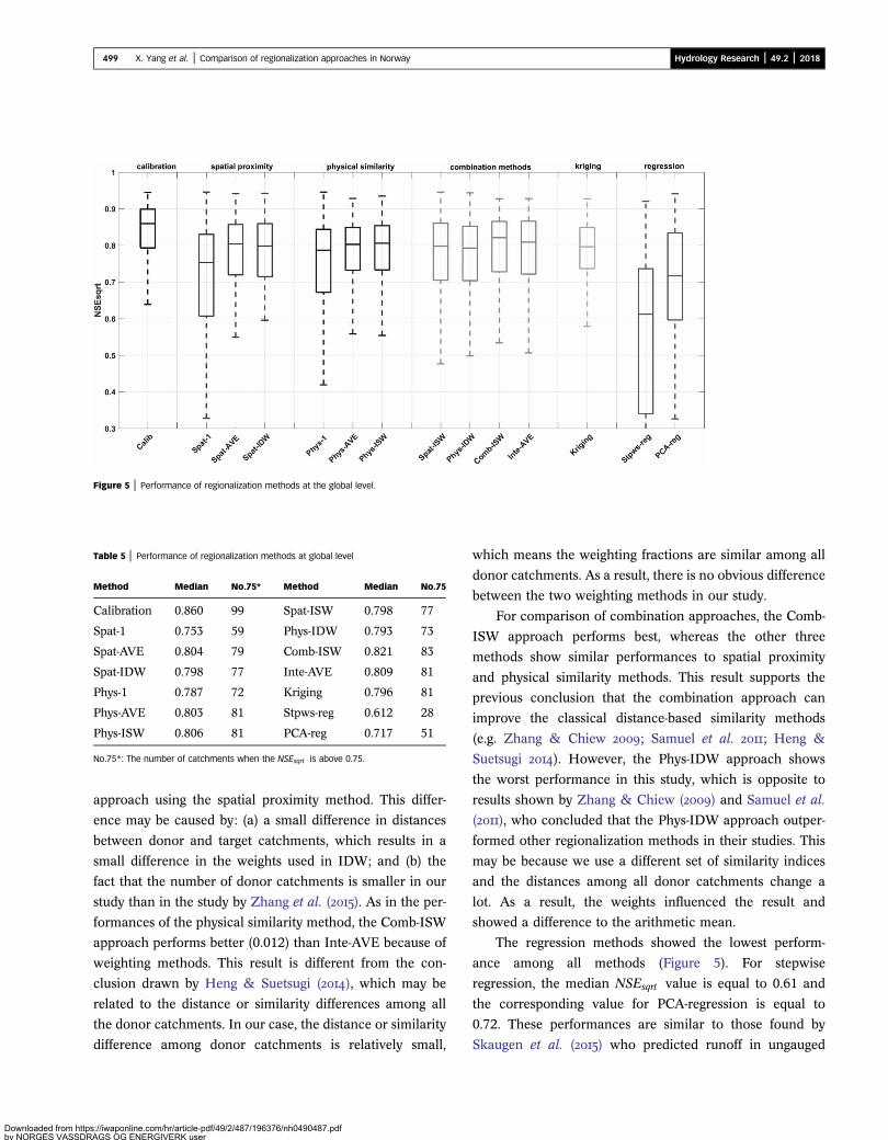
Figure 5 | Performance of regionalization methods at the global level.

Table 5 | Performance of regionalization methods at global level

Method Median No.75* Method Median No.75

Calibration 0.860 99 Spat-ISW 0.798 77

Spat-1 0.753 59 Phys-IDW 0.793 73

Spat-AVE 0.804 79 Comb-ISW 0.821 83

Spat-IDW 0.798 77 Inte-AVE 0.809 81

Phys-1 0.787 72 Kriging 0.796 81

Phys-AVE 0.803 81 Stpws-reg 0.612 28

Phys-ISW 0.806 81 PCA-reg 0.717 51

No.75*: The number of catchments when the NSEsqrt is above 0.75.



approach using the spatial proximity method. This differ-

ence may be caused by: (a) a small difference in distances

between donor and target catchments, which results in a

small difference in the weights used in IDW; and (b) the

fact that the number of donor catchments is smaller in our

study than in the study by Zhang et al. (). As in the per-

formances of the physical similarity method, the Comb-ISW

approach performs better (0.012) than Inte-AVE because of

weighting methods. This result is different from the con-

clusion drawn by Heng & Suetsugi (), which may be

related to the distance or similarity differences among all

the donor catchments. In our case, the distance or similarity

difference among donor catchments is relatively small,


which means the weighting fractions are similar among all

donor catchments. As a result, there is no obvious difference

between the two weighting methods in our study.

For comparison of combination approaches, the Comb-

ISW approach performs best, whereas the other three

methods show similar performances to spatial proximity

and physical similarity methods. This result supports the

previous conclusion that the combination approach can

improve the classical distance-based similarity methods

(e.g. Zhang & Chiew ; Samuel et al. ; Heng &

Suetsugi ). However, the Phys-IDW approach shows

the worst performance in this study, which is opposite to

results shown by Zhang & Chiew () and Samuel et al.

(), who concluded that the Phys-IDW approach outper-

formed other regionalization methods in their studies. This

may be because we use a different set of similarity indices

and the distances among all donor catchments change a

lot. As a result, the weights influenced the result and

showed a difference to the arithmetic mean.

The regression methods showed the lowest perform-

ance among all methods (Figure 5). For stepwise

regression, the median NSEsqrt value is equal to 0.61 and

the corresponding value for PCA-regression is equal to

0.72. These performances are similar to those found by

Skaugen et al. () who predicted runoff in ungauged

Figure 6 | Spatial distribution of best performing methods. For each catchment, the color

indicates which of the three standard regionalization methods (physical simi-

larity, regression, spatial proximity) produced the best results. Catchments

where the combination method outperformed the three other methods are

highlighted by a thick black border.



catchments in southern Norway by a multiple regression

method. In that study, they used a daily step, a parsimo-

nious rainfall-runoff model and built the regression

function using data from 84 catchments and tested in 17

independent catchments. Even though the datasets and

models are different, the performances are similar. The

PCA regression method produces a better result than step-

wise regression, likely because the PCA regression method

builds a relationship between model parameter values and

uncorrelated catchment descriptors.

For the difference in performance between Phys-ISW

and Comb-ISW, which is due to the inclusion of geographi-

cal distance in the Comb-ISWmethod, we can conclude that

the geographic distance plays a major role in regionaliza-

tion. This may be one of the reasons why spatial proximity

methods perform well in our case.

Summarizing our results at the global level, the best per-

formance is obtained by applying the combination method –

the Comb-ISW method – followed by a group of distance-

based similarity methods and Kriging, while the regression

methods showed the worst performance.

Figure 6 displays, for each catchment, which regionali-

zation method produced the best result. As with the

previous results, the spatial and physical similarity methods

show better results than the regression approach in most

watersheds. The regression method produces better results

than the remaining methods for a few catchments mainly

located at high elevations in the innermost parts of southern

Norway. The spatial proximity method shows the best per-

formance in 53 catchments, whereas the physical

similarity method outperforms the other methods in 46

catchments. Catchments where spatial proximity performs

best are mainly located in regions where the climate season-

ality and precipitation are close to the median for the whole

study region (climate seasonality index is on average 70 for

this group of catchments and annual mean precipitation is

1,842 mm). Meanwhile, the seasonality index rises to 88

and annual mean precipitation increases to 2,271 mm on

average for catchments where physical similarity performed

best. On the other hand, regression methods produced the

best simulations in catchments with low climate seasonality

(55 for mean climate seasonality index) and yearly precipi-

tation (1,630 mm). These catchments are located at the

highest mean elevation.


Note that even though we can identify the method that

performed best for each catchment from Figure 6, the aver-

age NSEsqrt difference between spatial proximity and

physical similarity methods is just about 0.06. This is poss-

ibly related to the low stream gauge network density in

our study, as it is not easy to decide which approach is the

most appropriate when the stream gauge network density

is lower than 60 stations per 100,000 km2 (Oudin et al.

).

Catchment classification

Figure 7 displays the result of the catchment classification

based on climate indices. The climate of catchments belong-

ing to groups 3 and 4 is characterized by larger precipitation

amounts and higher temperatures (see Figure 1 and Table 6).

Those watersheds are mainly located in the western parts of

southern Norway. Catchments in group 5 are exclusively

situated on higher elevations in southern Norway on the

Figure 7 | Climate regions classification in Norway.

Table 6 | Climate characteristics for different groups identified in the catchment

classification

Group1

Group2

Group3

Group4

Group5

Number of catchments 43 25 20 17 13

Precipitation(mm/month)

109 110 206 291 221

Temperature (�C) �0.03 2.82 4.18 3.79 0.16

Aridity index 0.13 0.25 0.13 0.08 0.05

Seasonality index 45.3 53 88 146 99

Area (km2) 453 547 129 127 111

Slope (�) 9.7 6.2 13.7 14 16

Elevation (m) 904 545.2 412 552 1,112

Normalized elevationrange*

1.41 1.85 2.08 1.40 0.56

*Normalized elevation range: Difference between maximum and minimum elevation

divided by mean elevation.

The numbers indicate the average values for each group.


Downloaded from https://iwaponline.com/hr/article-pdf/49/2/487/196376/nh0490487.pdfby NORGES VASSDRAGS OG ENERGIVERK useron 11 December 2018

transition zone where precipitation starts to decline from

west to east (see also Figure 1). Those catchments exhibit

higher precipitation amounts, whereas temperature is mark-

edly lower than for the watersheds in groups 3 and

4. Catchments in group 1 are located either in the mountai-

nous regions in southern Norway, or at higher latitudes

(above 68�N). The climate in those watersheds is dry and

cold. Finally, catchments in group 2 are mostly located in

the driest and relatively warm south-eastern parts of

Norway.

Assessment of regionalization methods using climate

regions

Figure 8 shows the NSEsqrt values from calibration and

global and regional regionalization results. The calibration

results show NSEsqrt values range between 0.76 and 0.89.

The highest median value is from group 5, which is 0.01

higher than group 1. The third ranked value is 0.86 for

group 4, being 0.04 higher than group 3. Group 2 displays

the lowest value.

Overall, selecting donor catchments from regions with a

similar climate does not strongly improve the model per-

formance. For the distance-based similarity methods,

group 5 produces the biggest difference while the differences

within the other four groups are relatively small. In most

cases, the regional results do not show better performance

than the global results, which means that the geographic fac-

tors are as important as climate factors in these kinds of

climate regions. For the regression methods, the differences

in median NSEsqrt value between the results of global and

regional regressions in all groups are within 0.02. The

global regression methods build the relationship based on

117 catchments and the regional regression methods use

information from catchments within each group to produce

the relationship. However, the difference between global

and regional result is small, which illustrates that the

regression methods are not strongly dependent on number

of catchments. For instance, there are only 13 catchments

in group 5 and both regional regression methods perform

with better results than the global regression methods.

The best performing method differs among the five

groups. For group 1 catchments, the regional Spat-AVE

approach produces the highest median NSEsqrt value and

Figure 8 | Comparison of NSEsqrt values for regionalization methods within five different climate regions.



combination approaches are on average better than other

methods. For group 2 catchments, the global Phys-AVE

approach is the best and physical similarity approaches

give similar simulations to combination approaches. The

global Inte-AVE approach performs the best in group 3

and most global approaches perform equally as well as

regional ones. For group 4 catchments, apart from

regression methods, the other methods all perform well

and the best performing approach is Comb-ISW. The Kri-

ging method performs robustly well for all groups; the

regional model parameter method performs better than

regression methods for most groups.

Generally, the distance-based similarity approaches per-

form much better than regression approaches in all groups.

In addition, the PCA regression approach produces accepta-

ble results (median NSEsqrt value is higher than 0.58).

Finally, the regional regression can further improve the

simulation if the global regression performs well, which

means that the linear relationship between model parameter

and catchment descriptors is validated. In general, the

results of regionalization methods in this study are better

than most of the similar studies reported in the literature,

confirming the hypothesis set up earlier that simple

models with statistically independent parameters are less


affected by equifinality and consequently have a better

chance to be successful for hydrological regionalization.

CONCLUSIONS

This study aims at evaluating the performances of regionali-

zation methods in Norway, a region located at high latitude,

characterized by a large climate gradient and with season-

ally snow-covered mountainous catchments. The

comparison was made at two levels: globally, over all catch-

ments in Norway; and regionally, in catchment groups

defined according to climate indices.

The study results show that the best regionalization

approach in Norway is the combination approach (Comb-

ISW), being slightly better than Kriging and other dis-

tance-based similarity approaches. The worst approach is

stepwise regression.

In this study, only the Comb-ISW approach showed

better simulation and the other three combination

approaches showed similar performances to classical

single approaches. All the distance-based similarity

approaches perform well in most humid regions in Norway.



The comparison of regionalization methods on the

regional and global levels shows that classifying catchments

into homogeneous groups before regionalization does not

improve the simulation in Norway, while it is worth testing

these conclusions in regions with more catchments and

different climate diversity.

ACKNOWLEDGEMENTS

This study is supported by Research and Development

Funding (Project number 80203) of the Norwegian Water

Resources and Energy Directorate (NVE), and by the

China Scholarship Council. We would like to thank the

NVE for providing the data for this study. We are thankful

to the three anonymous reviewers whose insightful and

constructive comments have led to a significant

improvement in the paper’s quality.

REFERENCES

Acreman, M. C. & Sinclair, C. D. Classification of drainagebasins according to their physical characteristics; anapplication for flood frequency analysis in Scotland.J. Hydrol. 84, 365–380.

Arora, V. K. The use of the aridity index to assess climatechange effect on annual runoff. J. Hydrol. 265, 164–177.doi:10.1016/S0022-1694(02)00101-4.

Arsenault, R., Poissant, D. & Brissette, F. Parameterdimensionality reduction of a conceptual model forstreamflow prediction in Canadian, snowmelt dominatedungauged basins. Adv. Water Resour. 85, 27–44. doi:10.1016/j.advwatres.2015.08.014.

Assunção, R. M., Neves, M. C., Câmara, G. & Da Costa Freitas, C. Efficient regionalization techniques for socio-economicgeographical units using minimum spanning trees.International Journal of Geographical Information Science 20(7), 797–811. https://doi.org/10.1080/13658810600665111.

Bao, Z., Zhang, J., Liu, J., Fu, G., Wang, G., He, R., Yan, X., Jin, J.& Liu, H. Comparison of regionalization approachesbased on regression and similarity for predictions inungauged catchments under multiple hydro-climaticconditions. J. Hydrol. 466–467, 37–46. doi:10.1016/j.jhydrol.2012.07.048.

Beldring, S., Engeland, K., Roald, L. A., Sælthun, N. R. & Voksø,A. Estimation of parameters in a distributedprecipitation-runoff model for Norway. Hydrology and Earth


System Sciences 7 (3), 304–316. https://doi.org/10.5194/hess-7-304-2003.

Blöschl, G. & Sivapalan, M. Scale issues in hydrologicalmodelling: A review. Hydrological Processes 9 (3–4), 251–290. https://doi.org/10.1002/hyp.3360090305

Budyko, M. I. Climate and Life. Academic Press, Orlando,FL, p. 508.

Bull, W. B. Tectonically Active Landscapes. Tectonically Act.Landscapes 1–326. doi:10.1002/9781444312003.

Burn, D. H. & Boorman, D. B. Estimation of hydrologicalparameters at ungauged catchments. J. Hydrol. 143, 429–454.doi:10.1016/0022-1694(93)90203-L.

Carvalho, M. J., Melo-Gonçalves, P., Teixeira, J. C. & Rocha, A. Regionalization of Europe based on a K-means clusteranalysis of the climate change of temperatures andprecipitation. Phys. Chem. Earth 94, 22–28. doi:10.1016/j.pce.2016.05.001.

Duque, J. C., Ramos, R. & Surinach, J. Supervisedregionalization methods: A survey. International RegionalScience Review 30 (3), 195–220. https://doi.org/10.1177/0160017607301605.

Egbuniwe, N. & Todd, D. K. Application of the StanfordWatershed Model to Nigerian watersheds. JAWRAJournal of the American Water Resources Association12 (3), 449–460. https://doi.org/10.1111/j.1752-1688.1976.tb02710.x

Elliot, W. Effects of forest biomass use on watershed processesin the Western United States. West. J. Appl. For. 25, 12–17.

Geological Survey of Norway (Norges geologiske undersøkelse) Product Specification: ND_Loads, Oslo, Norway.Retrieved from http://www.ngu.no/upload/Aktuelt/DOK_Produktspesifikasjon_Losmasser_ver3.pdf (accessed 2November 2016).

He, Y., Bárdossy, A. & Zehe, E. A review of regionalisation forcontinuous streamflow simulation. Hydrol. Earth Syst. Sci.15, 3539–3553. doi:10.5194/hess-15-3539-2011.

Heng, S. & Suetsugi, T. Comparison of regionalizationapproaches in parameterizing sediment rating curve inungauged catchments for subsequent instantaneous sedimentyield prediction. J. Hydrol. 512, 240–253. doi:10.1016/j.jhydrol.2014.03.003.

Hrachowitz, M., Savenije, H. H. G., Blöschl, G., McDonnell, J. J.,Sivapalan, M., Pomeroy, J. W., Arheimer, B., Blume, T., Clark,M. P., Ehret, U., Fenicia, F., Freer, J. E., Gelfan, A., Gupta,H.V.,Hughes,D.A.,Hut, R.W.,Montanari, A., Pande, S., Tetzlaff, D.,Troch, P. A., Uhlenbrook, S., Wagener, T., Winsemius, H. C.,Woods, R. A., Zehe, E. & Cudennec, C. A decade ofpredictions in ungauged basins (PUB)—a review. Hydrol. Sci. J.58, 1198–1255. doi:10.1080/02626667.2013.803183.

Hughes, D. A. Estimation of the parameters of an isolatedevent conceptual model from physical catchmentcharacteristics. Hydrological Sciences Journal 34 (5), 539–557. https://doi.org/10.1080/02626668909491361.

Hundecha, Y., Arheimer, B., Donnelly, C. & Pechlivanidis, I. A regional parameter estimation scheme for a pan-European

http://dx.doi.org/10.1016/0022-1694(86)90134-4

http://dx.doi.org/10.1016/0022-1694(86)90134-4

http://dx.doi.org/10.1016/0022-1694(86)90134-4

http://dx.doi.org/10.1016/S0022-1694(02)00101-4

http://dx.doi.org/10.1016/S0022-1694(02)00101-4

http://dx.doi.org/10.1016/j.advwatres.2015.08.014




http://dx.doi.org/10.1080/13658810600665111

http://dx.doi.org/10.1080/13658810600665111

http://dx.doi.org/10.1016/j.jhydrol.2012.07.048




http://dx.doi.org/10.5194/hess-7-304-2003


https://doi.org/10.1002/hyp.3360090305

https://doi.org/10.1002/hyp.3360090305

http://dx.doi.org/10.1016/0022-1694(93)90203-L

http://dx.doi.org/10.1016/0022-1694(93)90203-L

http://dx.doi.org/10.1016/j.pce.2016.05.001



http://dx.doi.org/10.1177/0160017607301605

http://dx.doi.org/10.1177/0160017607301605

http://dx.doi.org/10.1111/j.1752-1688.1976.tb02710.x

http://dx.doi.org/10.1111/j.1752-1688.1976.tb02710.x

http://www.ngu.no/upload/Aktuelt/DOK_Produktspesifikasjon_Losmasser_ver3.pdf









http://dx.doi.org/10.1080/02626667.2013.803183

http://dx.doi.org/10.1080/02626667.2013.803183

http://dx.doi.org/10.1080/02626668909491361

http://dx.doi.org/10.1080/02626668909491361

http://dx.doi.org/10.1080/02626668909491361

https://doi.org/10.1016/j.ejrh.2016.04.002



multi-basin model. Journal of Hydrology: Regional Studies 6,90–111. https://doi.org/10.1016/j.ejrh.2016.04.002.

Jarboe, J. E. & Haan, C. T. Calibrating a water yield model forsmall ungaged watersheds. Water Resources Research 10 (2),256–262. https://doi.org/10.1029/WR010i002p00256

Jones, J. R. Physical data for catchment models. NordicHydrology 7, 245–264.

Kay, A. L., Jones, D. A., Crooks, S. M., Kjeldsen, T. R. & Fung,C. F. An investigation of site-similarity approaches togeneralisation of a rainfall–runoff model. Hydrol. Earth Syst.Sci. 11, 500–515. doi:10.5194/hess-11-500-2007.

Kizza, M., Guerrero, J.-L., Rodhe, A., Xu, C.-Y. & Ntale, H. K. Modelling catchment inflows into Lake Victoria:regionalisation of the parameters of a conceptual waterbalance model. Hydrol. Res. 44 (5), 789–808.

Kokkonen, T. S., Jakeman, A. J., Young, P. C. & Koivusalo, H. J. Predicting daily flows in ungauged catchments: modelregionalization from catchment descriptors at the coweetahydrologic laboratory, North Carolina. Hydrol. Process. 17,2219–2238. doi:10.1002/hyp.1329.

Laaha, G. & Blöschl, G. A comparison of low flowregionalisation methods – catchment grouping. J. Hydrol.323, 193–214. doi:10.1016/j.jhydrol.2005.09.001.

Lagarias, J. C., Reeds, J. A., Wright, M. H. & Wright, P. E. Convergence properties of the Nelder-Mead simplex methodin low dimensions. SIAM Journal on Optimization, 9 (1),112–147. https://doi.org/10.1137/S1052623496303470.

Leclerc, M. & Ouarda, T. B. M. J. Non-stationary regionalflood frequency analysis at ungauged sites. J. Hydrol. 343,254–265. doi:10.1016/j.jhydrol.2007.06.021.

Li, L., Ngongondo, C. S., Xu, C.-Y. & Gong, L. Comparison ofthe global TRMM and WFD precipitation datasets in drivinga large-scale hydrological model in southern Africa.Hydrology Research 44 (5), 770–788. https://doi.org/10.2166/nh.2012.175.

Li, F., Zhang, Y., Xu, Z., Liu, C., Zhou, Y. & Liu, W. Runoffpredictions in ungauged catchments in southeast TibetanPlateau. J. Hydrol. 511, 28–38. doi:10.1016/j.jhydrol.2014.01.014.

Li, L., Diallo, I., Xu, C. Y. & Stordal, F. Hydrologicalprojections under climate change in the near future byRegCM4 in Southern Africa using a large-scale hydrologicalmodel. Journal of Hydrology 528, 1–16. https://doi.org/10.1016/j.jhydrol.2015.05.028

Liu, Y. & Gupta, H. V. Uncertainty in hydrologic modeling:toward an integrated data assimilation framework. WaterResour. Res. 43, 1–18. doi:10.1029/2006WR005756.

Magette, W. L., Shanholtz, V. O. & Carr, J. C. Estimatingselected parameters for the Kentucky Watershed Model fromwatershed characteristics. Water Resources Research 12 (3),472–476. https://doi.org/10.1029/WR012i003p00472

Matheron, G. The intrinsic random functions and theirapplications. Adv. Appl. Probab. 5, 439–468. doi:10.2307/1425829.


McIntyre, N., Lee, H., Wheater, H., Young, A. & Wagener, T. Ensemble predictions of runoff in ungauged catchments.Water Resour. Res. 41, 1–14. doi:10.1029/2005WR004289.

Merz, R. & Blöschl, G. Regionalisation of catchment modelparameters. J. Hydrol. 287, 95–123. doi:10.1016/j.jhydrol.2003.09.028.

Merz, R., Blöschl, G. & Parajka, J. Regionalisation methodsin rainfall-runoff modelling using large samples. Lr. ModelParam. Exp. IAHS Publ. 307, 117–125.

Müller-Wohlfeil, D.-I., Xu, C.-Y. & Iversen, H. L. Estimationof monthly river discharge from Danish catchments. NordicHydrology 34 (4), 295–320.

Oudin, L., Andréassian, V., Perrin, C., Michel, C. & Le Moine, N. Spatial proximity, physical similarity, regression andungauged catchments: a comparison of regionalizationapproaches based on 913 French catchments. Water Resour.Res. 44, 1–15. doi:10.1029/2007WR006240.

Parajka, J., Merz, R. & Blöschl, G. A comparison ofregionalisation methods for catchment model parameters.Hydrol. Earth Syst. Sci. Discuss. 2, 509–542. doi:10.5194/hessd-2-509-2005.

Parajka, J., Blöschl, G. & Merz, R. Regional calibration ofcatchment models: potential for ungauged catchments.WaterResour. Res. 43. doi:10.1029/2006WR005271.

Parajka, J., Viglione, A., Rogger, M., Salinas, J. L., Sivapalan, M. &Blöschl, G. Comparative assessment of predictions inungauged basins-Part 1: runoff-hydrograph studies. Hydrol.Earth Syst. Sci. 17, 1783–1795. doi:10.5194/hess-17-1783-2013.

Peña-Arancibia, J. L., Zhang, Y., Pagendam, D. E., Viney, N. R.,Lerat, J., van Dijk, A. I. J. M., Vaze, J. & Frost, A. J. Streamflow rating uncertainty: characterisation and impactson model calibration and performance. Environ. Model.Softw. 63, 32–44. doi:10.1016/j.envsoft.2014.09.011.

Pilgrim, D. H. Some problems in transferring hydrologicalrelationships between small and large drainage basins andbetween regions. J. Hydrol. 65, 49–72. doi:10.1016/0022-1694(83)90210-X.

Razavi, T. & Coulibaly, P. Streamflow prediction in ungaugedbasins: review of regionalization methods. J. Hydrol. Eng. 18,958–975. doi:10.1061/(ASCE)HE.1943-5584.0000690.

Reichl, J. P. C., Western, A. W., McIntyre, N. R. & Chiew, F. H. S. Optimization of a similarity measure for estimatingungauged streamflow. Water Resour. Res. 45, 1–15. doi:10.1029/2008WR007248.

Ross, W. The relative roles of climate, soil, vegetation andtopography in determining seasonal and long-termcatchment dynamics. Adv. Water Resour. 30, 1061. doi:10.1016/j.advwatres.2006.10.010.

Salinas, J. L., Laaha,G.,Rogger,M., Parajka, J.,Viglione,A., Sivapalan,M. & Blöschl, G. Comparative assessment of predictions inungaugedbasins-Part 2:floodand lowflowstudies.Hydrol. EarthSyst. Sci. 17, 2637–2652. doi:10.5194/hess-17-2637-2013.

Samuel, J., Coulibaly, P. & Metcalfe, R. A. Estimation ofcontinuous streamflow in Ontario ungauged basins:

https://doi.org/10.1016/j.ejrh.2016.04.002

http://dx.doi.org/10.1029/WR010i002p00256




http://dx.doi.org/10.2166/nh.2012.152

http://dx.doi.org/10.2166/nh.2012.152

http://dx.doi.org/10.2166/nh.2012.152

http://dx.doi.org/10.1002/hyp.1329





http://dx.doi.org/10.1137/S1052623496303470

http://dx.doi.org/10.1137/S1052623496303470



http://dx.doi.org/10.2166/nh.2012.175

http://dx.doi.org/10.2166/nh.2012.175

http://dx.doi.org/10.2166/nh.2012.175








http://dx.doi.org/10.1029/2006WR005756

http://dx.doi.org/10.1029/2006WR005756




http://dx.doi.org/10.1017/S0001867800039379

http://dx.doi.org/10.1017/S0001867800039379

http://dx.doi.org/10.1029/2005WR004289



http://dx.doi.org/10.1029/2007WR006240

http://dx.doi.org/10.1029/2007WR006240

http://dx.doi.org/10.1029/2007WR006240

http://dx.doi.org/10.5194/hessd-2-509-2005

http://dx.doi.org/10.5194/hessd-2-509-2005

http://dx.doi.org/10.1029/2006WR005271

http://dx.doi.org/10.1029/2006WR005271



http://dx.doi.org/10.1016/j.envsoft.2014.09.011

http://dx.doi.org/10.1016/j.envsoft.2014.09.011

http://dx.doi.org/10.1016/0022-1694(83)90210-X

http://dx.doi.org/10.1016/0022-1694(83)90210-X

http://dx.doi.org/10.1016/0022-1694(83)90210-X

http://dx.doi.org/10.1061/(ASCE)HE.1943-5584.0000690


http://dx.doi.org/10.1029/2008WR007248

http://dx.doi.org/10.1029/2008WR007248










comparison of regionalization methods. J. Hydrol. Eng. 16,447–459. doi:10.1061/(ASCE)HE.1943-5584.0000338.

Samuel, J., Coulibaly, P. & Metcalfe, R. A. Evaluation offuture flow variability in ungauged basins: validation ofcombined methods. Adv. Water Resour. 35, 121–140. doi:10.1016/j.advwatres.2011.09.015.

Sefton, C. E. M. & Howarth, S. M. Relationships betweendynamic response characteristics and physical descriptors ofcatchments in England and Wales. Journal of Hydrology 211(1–4), 1–16. https://doi.org/10.1016/S0022-1694(98)00163-2.

Seibert, J. Regionalisation of parameters for a conceptualrainfall-runoff model. Agricultural and Forest Meteorology98–99, 279–293. https://doi.org/10.1016/S0168-1923,(99)00105-7.

Seibert, J. & Beven, K. J. Gauging the ungauged basin: howmany discharge measurements are needed? Hydrology andEarth System Sciences 13, 883–892. https://doi.org/10.5194/hessd-6-2275-2009.

Seiller, G., Anctil, F. & Perrin, C. Multimodel evaluation oftwenty lumped hydrological models under contrasted climateconditions. Hydrol. Earth Syst. Sci. 16, 1171–1189. doi:10.5194/hess-16-1171-2012.

Servat, E. & Dezetter, A. Rainfall-runoff modelling and waterresources assessment in northwestern Ivory Coast. Tentativeextension to ungauged catchments. Journal of Hydrology 148(1–4), 231–248. https://doi.org/10.1016/0022-1694(93)90262-8

Sivapalan, M., Takeuchi, K., Franks, S. W., Gupta, V. K.,Karambiri, H., Lakshmi, V., Liang, X., McDonnell, J. J.,Mendiondo, E. M., O’Connell, P. E., Oki, T., Pomeroy, J. W.,Schertzer, D., Uhlenbrook, S. & Zehe, E. IAHS Decadeon Predictions in Ungauged Basins (PUB), 2003–2012:Shaping an exciting future for the hydrological sciences.Hydrological Sciences Journal 48 (6), 857–880. https://doi.org/10.1623/hysj.48.6.857.51421

Skaugen, T., Peerebom, I. O. & Nilsson, A. Use of aparsimonious rainfall-run-off model for predictinghydrological response in ungauged basins. Hydrol. Process.29, 1999–2013. doi:10.1002/hyp.10315.

Ssegane, H., Tollner, E. W., Mohamoud, Y. M., Rasmussen, T. C.& Dowd, J. F. Advances in variable selection methods I:causal selection methods versus stepwise regression andprincipal component analysis on data of known andunknown functional relationships. J. Hydrol. 438–439, 16–25.doi:10.1016/j.jhydrol.2012.01.008.

Vandewiele, G. L. & Elias, A. Monthly water balance ofungauged catchments obtained by geographical regionalization.J. Hydrol. 170, 277–291. doi:10.1016/0022-1694(95)02681-E.

Vandewiele, G. L., Xu, C.-Y. & Huybrechts, W. Regionalisation of physically-based water balance models inBelgium. application to ungauged catchments. Water Resour.Manag. 5, 199–208. doi:10.1007/BF00421989.


Vandewiele, G. L., Xu, C.-Y. & Ni-Lar-Win, Methodology andcomparative study on monthly water balance models inBelgium, China and Burma. J. Hydrol. 134, 315–347.

Viglione,A., Parajka, J., Rogger,M., Salinas, J. L., Laaha,G., Sivapalan,M. & Blöschl, G. Comparative assessment of predictions inungauged basins – part 3: runoff signatures in Austria. Hydrol.Earth Syst. Sci. 17, 2263–2279. doi:10.5194/hess-17-2263-2013.

Vormoor, K., Skaugen, T., Langsholt, E., Diekkrüger, B. & Skøien,J. O. Geostatistical regionalization of daily runoffforecasts in Norway. Int. J. River Basin Manag. 9, 3–15.doi:10.1080/15715124.2010.543905.

Wagener, T., Sivapalan, M., Troch, P. & Woods, R. Catchment classification and hydrologic similarity.Geography Compass 1, 1–31. https://doi.org/10.1111/j.1749-8198.2007.00039.x

Widén-Nilsson, E., Halldin, S. & Xu, C.-Y. Global water-balance modelling with WASMOD-M: parameter estimationand regionalisation. J. Hydrol. 340, 105–118. doi:10.1016/j.jhydrol.2007.04.002.

Xu, C.-Y. Application of water balance models to differentclimatic regions in China for water resources assessment.Water Resour. Manag. 11, 51–67.

Xu, C.-Y. a Estimation of parameters of a conceptual waterbalance model for ungauged catchments. Water Resour.Manag. 13 (5), 353–368.

Xu, C.-Y. b Operational testing of a water balance model forpredicting climate change impacts. Agricultural and ForestMeteorology 98–99 (1–4), 295–304.

Xu, C.-Y. Statistical analysis of a conceptual water balancemodel, methodology and case study. Water Resour. Manag.15, 75–92.

Xu, C.-Y. WAS-MOD The water and snow balance modelingsystem. In: Mathematical Models of Small WatershedHydrology and Applications, Chapter 17 (V. P. Singh & D. K.Frevert, eds). Water Resources Publications, LLC, Colorado,USA, pp. 555–590.

Xu, C.-Y. Testing the transferability of regression equationsderived from small sub-catchments to a large area in centralSweden. Hydrol. Earth Syst. Sci. 7, 317–324. doi:10.5194/hess-7-317-2003.

Young, A. R. Stream flow simulation withinUK ungauged catchments using a daily rainfall-runoff model.J. Hydrol. 320, 155–172. doi:10.1016/j.jhydrol.2005.07.017.

Zhang, Y. & Chiew, F. Evaluation of regionalization methodsfor predicting runoff in ungauged catchments in SoutheastAustralia. In: 18th World IMACS/MODSIM Congress,Cairns, Australia, pp. 3442–3448.

Zhang, Y., Vaze, J., Chiew, F. H. S. & Li, M. Comparing flowduration curve and rainfall-runoff modelling for predictingdaily runoff in ungauged catchments. J. Hydrol. 525, 72–86.doi:10.1016/j.jhydrol.2015.03.043.

First received 5 April 2017; accepted in revised form 1 November 2017. Available online 5 December 2017





http://dx.doi.org/10.1016/S0022-1694(98)00163-2

http://dx.doi.org/10.1016/S0022-1694(98)00163-2

http://dx.doi.org/10.1016/S0022-1694(98)00163-2

http://dx.doi.org/10.1016/S0168-1923(99)00105-7

http://dx.doi.org/10.1016/S0168-1923(99)00105-7






http://dx.doi.org/10.1016/0022-1694(93)90262-8

http://dx.doi.org/10.1016/0022-1694(93)90262-8

http://dx.doi.org/10.1016/0022-1694(93)90262-8

http://dx.doi.org/10.1623/hysj.48.6.857.51421










http://dx.doi.org/10.1016/0022-1694(95)02681-E

http://dx.doi.org/10.1016/0022-1694(95)02681-E

http://dx.doi.org/10.1007/BF00421989

http://dx.doi.org/10.1007/BF00421989

http://dx.doi.org/10.1016/0022-1694(92)90041-S

http://dx.doi.org/10.1016/0022-1694(92)90041-S

http://dx.doi.org/10.1016/0022-1694(92)90041-S



http://dx.doi.org/10.1080/15715124.2010.543905

http://dx.doi.org/10.1080/15715124.2010.543905

http://dx.doi.org/10.1111/j.1749-8198.2007.00039.x




http://dx.doi.org/10.1023/A:1007945406728

http://dx.doi.org/10.1023/A:1007945406728

http://dx.doi.org/10.1023/A:1008191517801

http://dx.doi.org/10.1023/A:1008191517801

http://dx.doi.org/10.1016/S0168-1923(99)00106-9

http://dx.doi.org/10.1016/S0168-1923(99)00106-9

http://dx.doi.org/10.1023/A:1012559608269

http://dx.doi.org/10.1023/A:1012559608269









runoff prediction in ungauged catchments in norway

Documents