sage reference manual: functionsdoc.sagemath.org/pdf/en/reference/functions/functions.pdf ·...
TRANSCRIPT

Sage Reference Manual: FunctionsRelease 9.0
The Sage Development Team
Jan 01, 2020


CONTENTS
1 Built-in Functions 11.1 Logarithmic Functions . . . . . . . . . . . . . . . . . . . . . . . . . . . . . . . . . . . . . . . . . . 11.2 Trigonometric Functions . . . . . . . . . . . . . . . . . . . . . . . . . . . . . . . . . . . . . . . . . 101.3 Hyperbolic Functions . . . . . . . . . . . . . . . . . . . . . . . . . . . . . . . . . . . . . . . . . . 201.4 Number-Theoretic Functions . . . . . . . . . . . . . . . . . . . . . . . . . . . . . . . . . . . . . . . 281.5 Error Functions . . . . . . . . . . . . . . . . . . . . . . . . . . . . . . . . . . . . . . . . . . . . . . 331.6 Piecewise-defined Functions . . . . . . . . . . . . . . . . . . . . . . . . . . . . . . . . . . . . . . . 361.7 Spike Functions . . . . . . . . . . . . . . . . . . . . . . . . . . . . . . . . . . . . . . . . . . . . . 471.8 Orthogonal Polynomials . . . . . . . . . . . . . . . . . . . . . . . . . . . . . . . . . . . . . . . . . 491.9 Other functions . . . . . . . . . . . . . . . . . . . . . . . . . . . . . . . . . . . . . . . . . . . . . . 601.10 Miscellaneous Special Functions . . . . . . . . . . . . . . . . . . . . . . . . . . . . . . . . . . . . 721.11 Hypergeometric Functions . . . . . . . . . . . . . . . . . . . . . . . . . . . . . . . . . . . . . . . . 771.12 Jacobi Elliptic Functions . . . . . . . . . . . . . . . . . . . . . . . . . . . . . . . . . . . . . . . . . 861.13 Airy Functions . . . . . . . . . . . . . . . . . . . . . . . . . . . . . . . . . . . . . . . . . . . . . . 891.14 Bessel Functions . . . . . . . . . . . . . . . . . . . . . . . . . . . . . . . . . . . . . . . . . . . . . 941.15 Exponential Integrals . . . . . . . . . . . . . . . . . . . . . . . . . . . . . . . . . . . . . . . . . . . 1091.16 Wigner, Clebsch-Gordan, Racah, and Gaunt coefficients . . . . . . . . . . . . . . . . . . . . . . . . 1201.17 Generalized Functions . . . . . . . . . . . . . . . . . . . . . . . . . . . . . . . . . . . . . . . . . . 1271.18 Counting Primes . . . . . . . . . . . . . . . . . . . . . . . . . . . . . . . . . . . . . . . . . . . . . 1301.19 Symbolic Minimum and Maximum . . . . . . . . . . . . . . . . . . . . . . . . . . . . . . . . . . . 133
2 Indices and Tables 135
Python Module Index 137
Index 139
i

ii

CHAPTER
ONE
BUILT-IN FUNCTIONS
1.1 Logarithmic Functions
AUTHORS:
• Yoora Yi Tenen (2012-11-16): Add documentation for log() (trac ticket #12113)
• Tomas Kalvoda (2015-04-01): Add exp_polar() (trac ticket #18085)
class sage.functions.log.Function_dilogBases: sage.symbolic.function.GinacFunction
The dilogarithm function Li2(𝑧) =∑∞
𝑘=1 𝑧𝑘/𝑘2.
This is simply an alias for polylog(2, z).
EXAMPLES:
sage: dilog(1)1/6*pi^2sage: dilog(1/2)1/12*pi^2 - 1/2*log(2)^2sage: dilog(x^2+1)dilog(x^2 + 1)sage: dilog(-1)-1/12*pi^2sage: dilog(-1.0)-0.822467033424113sage: dilog(-1.1)-0.890838090262283sage: dilog(1/2)1/12*pi^2 - 1/2*log(2)^2sage: dilog(.5)0.582240526465012sage: dilog(1/2).n()0.582240526465012sage: var('z')zsage: dilog(z).diff(z, 2)log(-z + 1)/z^2 - 1/((z - 1)*z)sage: dilog(z).series(z==1/2, 3)(1/12*pi^2 - 1/2*log(2)^2) + (-2*log(1/2))*(z - 1/2) + (2*log(1/2) +→˓2)*(z - 1/2)^2 + Order(1/8*(2*z - 1)^3)
sage: latex(dilog(z))\rm Li_2\left(z\right)
1

Sage Reference Manual: Functions, Release 9.0
Dilog has a branch point at 1. Sage’s floating point libraries may handle this differently from thesymbolic package:
sage: dilog(1)1/6*pi^2sage: dilog(1.)1.64493406684823sage: dilog(1).n()1.64493406684823sage: float(dilog(1))1.6449340668482262
class sage.functions.log.Function_expBases: sage.symbolic.function.GinacFunction
The exponential function, exp(𝑥) = 𝑒𝑥.
EXAMPLES:
sage: exp(-1)e^(-1)sage: exp(2)e^2sage: exp(2).n(100)7.3890560989306502272304274606sage: exp(x^2 + log(x))e^(x^2 + log(x))sage: exp(x^2 + log(x)).simplify()x*e^(x^2)sage: exp(2.5)12.1824939607035sage: exp(float(2.5))12.182493960703473sage: exp(RDF('2.5'))12.182493960703473sage: exp(I*pi/12)(1/4*I + 1/4)*sqrt(6) - (1/4*I - 1/4)*sqrt(2)
To prevent automatic evaluation, use the hold parameter:
sage: exp(I*pi,hold=True)e^(I*pi)sage: exp(0,hold=True)e^0
To then evaluate again, we currently must use Maxima via sage.symbolic.expression.Expression.simplify():
sage: exp(0,hold=True).simplify()1
sage: exp(pi*I/2)Isage: exp(pi*I)-1sage: exp(8*pi*I)1
(continues on next page)
2 Chapter 1. Built-in Functions

Sage Reference Manual: Functions, Release 9.0
(continued from previous page)
sage: exp(7*pi*I/2)-I
For the sake of simplification, the argument is reduced modulo the period of the complex exponential function,2𝜋𝑖:
sage: k = var('k', domain='integer')sage: exp(2*k*pi*I)1sage: exp(log(2) + 2*k*pi*I)2
The precision for the result is deduced from the precision of the input. Convert the input to a higher precisionexplicitly if a result with higher precision is desired:
sage: t = exp(RealField(100)(2)); t7.3890560989306502272304274606sage: t.prec()100sage: exp(2).n(100)7.3890560989306502272304274606
class sage.functions.log.Function_exp_polarBases: sage.symbolic.function.BuiltinFunction
Representation of a complex number in a polar form.
INPUT:
• z - a complex number 𝑧 = 𝑎 + 𝑖𝑏.
OUTPUT:
A complex number with modulus exp(𝑎) and argument 𝑏.
If −𝜋 < 𝑏 ≤ 𝜋 then exp_polar(𝑧) = exp(𝑧). For other values of 𝑏 the function is left unevaluated.
EXAMPLES:
The following expressions are evaluated using the exponential function:
sage: exp_polar(pi*I/2)Isage: x = var('x', domain='real')sage: exp_polar(-1/2*I*pi + x)e^(-1/2*I*pi + x)
The function is left unevaluated when the imaginary part of the input 𝑧 does not satisfy −𝜋 < ℑ(𝑧) ≤ 𝜋:
sage: exp_polar(2*pi*I)exp_polar(2*I*pi)sage: exp_polar(-4*pi*I)exp_polar(-4*I*pi)
This fixes trac ticket #18085:
sage: integrate(1/sqrt(1+x^3),x,algorithm='sympy')1/3*x*gamma(1/3)*hypergeometric((1/3, 1/2), (4/3,), -x^3)/gamma(4/3)
1.1. Logarithmic Functions 3
Sage Reference Manual: Functions, Release 9.0
See also:
Examples in Sympy documentation, Sympy source code of exp_polar
REFERENCES:
Wikipedia article Complex_number#Polar_form
class sage.functions.log.Function_harmonic_numberBases: sage.symbolic.function.BuiltinFunction
Harmonic number function, defined by:
𝐻𝑛 = 𝐻𝑛,1 =
𝑛∑𝑘=1
1
𝑘
𝐻𝑠 =
∫ 1
0
1 − 𝑥𝑠
1 − 𝑥
See the docstring for Function_harmonic_number_generalized().
This class exists as callback for harmonic_number returned by Maxima.
class sage.functions.log.Function_harmonic_number_generalizedBases: sage.symbolic.function.BuiltinFunction
Harmonic and generalized harmonic number functions, defined by:
𝐻𝑛 = 𝐻𝑛,1 =
𝑛∑𝑘=1
1
𝑘
𝐻𝑛,𝑚 =
𝑛∑𝑘=1
1
𝑘𝑚
They are also well-defined for complex argument, through:
𝐻𝑠 =
∫ 1
0
1 − 𝑥𝑠
1 − 𝑥
𝐻𝑠,𝑚 = 𝜁(𝑚) − 𝜁(𝑚, 𝑠− 1)
If called with a single argument, that argument is s and m is assumed to be 1 (the normal harmonic numbersH_s).
ALGORITHM:
Numerical evaluation is handled using the mpmath and FLINT libraries.
REFERENCES:
• Wikipedia article Harmonic_number
EXAMPLES:
Evaluation of integer, rational, or complex argument:
sage: harmonic_number(5)137/60sage: harmonic_number(3,3)251/216sage: harmonic_number(5/2)-2*log(2) + 46/15sage: harmonic_number(3.,3)
(continues on next page)
4 Chapter 1. Built-in Functions

Sage Reference Manual: Functions, Release 9.0
(continued from previous page)
zeta(3) - 0.0400198661225573sage: harmonic_number(3.,3.)1.16203703703704sage: harmonic_number(3,3).n(200)1.16203703703703703703703...sage: harmonic_number(1+I,5)harmonic_number(I + 1, 5)sage: harmonic_number(5,1.+I)1.57436810798989 - 1.06194728851357*I
Solutions to certain sums are returned in terms of harmonic numbers:
sage: k=var('k')sage: sum(1/k^7,k,1,x)harmonic_number(x, 7)
Check the defining integral at a random integer:
sage: n=randint(10,100)sage: bool(SR(integrate((1-x^n)/(1-x),x,0,1)) == harmonic_number(n))True
There are several special values which are automatically simplified:
sage: harmonic_number(0)0sage: harmonic_number(1)1sage: harmonic_number(x,1)harmonic_number(x)
Arguments are swapped with respect to the same functions in Maxima:
sage: maxima(harmonic_number(x,2)) # maxima expect interfacegen_harmonic_number(2,_SAGE_VAR_x)sage: from sage.calculus.calculus import symbolic_expression_from_maxima_string→˓as sefmssage: sefms('gen_harmonic_number(3,x)')harmonic_number(x, 3)sage: from sage.interfaces.maxima_lib import maxima_lib, max_to_srsage: c=maxima_lib(harmonic_number(x,2)); cgen_harmonic_number(2,_SAGE_VAR_x)sage: max_to_sr(c.ecl())harmonic_number(x, 2)
class sage.functions.log.Function_lambert_wBases: sage.symbolic.function.BuiltinFunction
The integral branches of the Lambert W function 𝑊𝑛(𝑧).
This function satisfies the equation
𝑧 = 𝑊𝑛(𝑧)𝑒𝑊𝑛(𝑧)
INPUT:
• n - an integer. 𝑛 = 0 corresponds to the principal branch.
• z - a complex number
1.1. Logarithmic Functions 5

Sage Reference Manual: Functions, Release 9.0
If called with a single argument, that argument is z and the branch n is assumed to be 0 (the principal branch).
ALGORITHM:
Numerical evaluation is handled using the mpmath and SciPy libraries.
REFERENCES:
• Wikipedia article Lambert_W_function
EXAMPLES:
Evaluation of the principal branch:
sage: lambert_w(1.0)0.567143290409784sage: lambert_w(-1).n()-0.318131505204764 + 1.33723570143069*Isage: lambert_w(-1.5 + 5*I)1.17418016254171 + 1.10651494102011*I
Evaluation of other branches:
sage: lambert_w(2, 1.0)-2.40158510486800 + 10.7762995161151*I
Solutions to certain exponential equations are returned in terms of lambert_w:
sage: S = solve(e^(5*x)+x==0, x, to_poly_solve=True)sage: z = S[0].rhs(); z-1/5*lambert_w(5)sage: N(z)-0.265344933048440
Check the defining equation numerically at 𝑧 = 5:
sage: N(lambert_w(5)*exp(lambert_w(5)) - 5)0.000000000000000
There are several special values of the principal branch which are automatically simplified:
sage: lambert_w(0)0sage: lambert_w(e)1sage: lambert_w(-1/e)-1
Integration (of the principal branch) is evaluated using Maxima:
sage: integrate(lambert_w(x), x)(lambert_w(x)^2 - lambert_w(x) + 1)*x/lambert_w(x)sage: integrate(lambert_w(x), x, 0, 1)(lambert_w(1)^2 - lambert_w(1) + 1)/lambert_w(1) - 1sage: integrate(lambert_w(x), x, 0, 1.0)0.3303661247616807
Warning: The integral of a non-principal branch is not implemented, neither is numerical integration using GSL.The numerical_integral() function does work if you pass a lambda function:
6 Chapter 1. Built-in Functions

Sage Reference Manual: Functions, Release 9.0
sage: numerical_integral(lambda x: lambert_w(x), 0, 1)(0.33036612476168054, 3.667800782666048e-15)
class sage.functions.log.Function_log1Bases: sage.symbolic.function.GinacFunction
The natural logarithm of x.
See log() for extensive documentation.
EXAMPLES:
sage: ln(e^2)2sage: ln(2)log(2)sage: ln(10)log(10)
class sage.functions.log.Function_log2Bases: sage.symbolic.function.GinacFunction
Return the logarithm of x to the given base.
See log() for extensive documentation.
EXAMPLES:
sage: from sage.functions.log import logbsage: logb(1000,10)3
class sage.functions.log.Function_polylogBases: sage.symbolic.function.GinacFunction
The polylog function Li𝑠(𝑧) =∑∞
𝑘=1 𝑧𝑘/𝑘𝑠.
This definition is valid for arbitrary complex order 𝑠 and for all complex arguments 𝑧 with |𝑧| < 1; it can beextended to |𝑧| ≥ 1 by the process of analytic continuation. So the function may have a discontinuity at 𝑧 = 1which can cause a 𝑁𝑎𝑁 value returned for floating point arguments.
EXAMPLES:
sage: polylog(2.7, 0)0.000000000000000sage: polylog(2, 1)1/6*pi^2sage: polylog(2, -1)-1/12*pi^2sage: polylog(3, -1)-3/4*zeta(3)sage: polylog(2, I)I*catalan - 1/48*pi^2sage: polylog(4, 1/2)polylog(4, 1/2)sage: polylog(4, 0.5)0.517479061673899
sage: polylog(1, x)-log(-x + 1)
(continues on next page)
1.1. Logarithmic Functions 7

Sage Reference Manual: Functions, Release 9.0
(continued from previous page)
sage: polylog(2,x^2+1)dilog(x^2 + 1)
sage: f = polylog(4, 1); f1/90*pi^4sage: f.n()1.08232323371114
sage: polylog(4, 2).n()2.42786280675470 - 0.174371300025453*Isage: complex(polylog(4,2))(2.4278628067547032-0.17437130002545306j)sage: float(polylog(4,0.5))0.5174790616738993
sage: z = var('z')sage: polylog(2,z).series(z==0, 5)1*z + 1/4*z^2 + 1/9*z^3 + 1/16*z^4 + Order(z^5)
sage: loads(dumps(polylog))polylog
sage: latex(polylog(5, x))\rm Li_5(x)sage: polylog(x, x)._sympy_()polylog(x, x)
sage.functions.log.log(*args, **kwds)Return the logarithm of the first argument to the base of the second argument which if missing defaults to e.
It calls the log method of the first argument when computing the logarithm, thus allowing the use of logarithmon any object containing a log method. In other words, log works on more than just real numbers.
EXAMPLES:
sage: log(e^2)2
To change the base of the logarithm, add a second parameter:
sage: log(1000,10)3
The synonym ln can only take one argument:
sage: ln(RDF(10))2.302585092994046sage: ln(2.718)0.999896315728952sage: ln(2.0)0.693147180559945sage: ln(float(-1))3.141592653589793jsage: ln(complex(-1))3.141592653589793j
You can use RDF, RealField or n to get a numerical real approximation:
8 Chapter 1. Built-in Functions
Sage Reference Manual: Functions, Release 9.0
sage: log(1024, 2)10sage: RDF(log(1024, 2))10.0sage: log(10, 4)1/2*log(10)/log(2)sage: RDF(log(10, 4))1.6609640474436813sage: log(10, 2)log(10)/log(2)sage: n(log(10, 2))3.32192809488736sage: log(10, e)log(10)sage: n(log(10, e))2.30258509299405
The log function works for negative numbers, complex numbers, and symbolic numbers too, picking the branchwith angle between −𝜋 and 𝜋:
sage: log(-1+0*I)I*pisage: log(CC(-1))3.14159265358979*Isage: log(-1.0)3.14159265358979*I
Small integer powers are factored out immediately:
sage: log(4)2*log(2)sage: log(1000000000)9*log(10)sage: log(8) - 3*log(2)0sage: bool(log(8) == 3*log(2))True
The hold parameter can be used to prevent automatic evaluation:
sage: log(-1,hold=True)log(-1)sage: log(-1)I*pisage: I.log(hold=True)log(I)sage: I.log(hold=True).simplify()1/2*I*pi
For input zero, the following behavior occurs:
sage: log(0)-Infinitysage: log(CC(0))-infinitysage: log(0.0)-infinity
1.1. Logarithmic Functions 9

Sage Reference Manual: Functions, Release 9.0
The log function also works in finite fields as long as the argument lies in the multiplicative group generated bythe base:
sage: F = GF(13); g = F.multiplicative_generator(); g2sage: a = F(8)sage: log(a,g); g^log(a,g)38sage: log(a,3)Traceback (most recent call last):...ValueError: No discrete log of 8 found to base 3 modulo 13sage: log(F(9), 3)2
The log function also works for p-adics (see documentation for p-adics for more information):
sage: R = Zp(5); R5-adic Ring with capped relative precision 20sage: a = R(16); a1 + 3*5 + O(5^20)sage: log(a)3*5 + 3*5^2 + 3*5^4 + 3*5^5 + 3*5^6 + 4*5^7 + 2*5^8 + 5^9 +5^11 + 2*5^12 + 5^13 + 3*5^15 + 2*5^16 + 4*5^17 + 3*5^18 +3*5^19 + O(5^20)
1.2 Trigonometric Functions
class sage.functions.trig.Function_arccosBases: sage.symbolic.function.GinacFunction
The arccosine function.
EXAMPLES:
sage: arccos(0.5)1.04719755119660sage: arccos(1/2)1/3*pisage: arccos(1 + 1.0*I)0.904556894302381 - 1.06127506190504*Isage: arccos(3/4).n(100)0.72273424781341561117837735264
We can delay evaluation using the hold parameter:
sage: arccos(0,hold=True)arccos(0)
To then evaluate again, we currently must use Maxima via sage.symbolic.expression.Expression.simplify():
sage: a = arccos(0,hold=True); a.simplify()1/2*pi
10 Chapter 1. Built-in Functions

Sage Reference Manual: Functions, Release 9.0
conjugate(arccos(x))==arccos(conjugate(x)), unless on the branch cuts, which run along thereal axis outside the interval [-1, +1].:
sage: conjugate(arccos(x))conjugate(arccos(x))sage: var('y', domain='positive')ysage: conjugate(arccos(y))conjugate(arccos(y))sage: conjugate(arccos(y+I))conjugate(arccos(y + I))sage: conjugate(arccos(1/16))arccos(1/16)sage: conjugate(arccos(2))conjugate(arccos(2))sage: conjugate(arccos(-2))pi - conjugate(arccos(2))
class sage.functions.trig.Function_arccotBases: sage.symbolic.function.GinacFunction
The arccotangent function.
EXAMPLES:
sage: arccot(1/2)arccot(1/2)sage: RDF(arccot(1/2)) # abs tol 2e-161.1071487177940906sage: arccot(1 + I)arccot(I + 1)sage: arccot(1/2).n(100)1.1071487177940905030170654602sage: float(arccot(1/2)) # abs tol 2e-161.1071487177940906sage: bool(diff(acot(x), x) == -diff(atan(x), x))Truesage: diff(acot(x), x)-1/(x^2 + 1)
We can delay evaluation using the hold parameter:
sage: arccot(1,hold=True)arccot(1)
To then evaluate again, we currently must use Maxima via sage.symbolic.expression.Expression.simplify():
sage: a = arccot(1,hold=True); a.simplify()1/4*pi
class sage.functions.trig.Function_arccscBases: sage.symbolic.function.GinacFunction
The arccosecant function.
EXAMPLES:
1.2. Trigonometric Functions 11

Sage Reference Manual: Functions, Release 9.0
sage: arccsc(2)arccsc(2)sage: RDF(arccsc(2)) # rel tol 1e-150.5235987755982988sage: arccsc(2).n(100)0.52359877559829887307710723055sage: float(arccsc(2))0.52359877559829...sage: arccsc(1 + I)arccsc(I + 1)sage: diff(acsc(x), x)-1/(sqrt(x^2 - 1)*x)sage: arccsc(x)._sympy_()acsc(x)
We can delay evaluation using the hold parameter:
sage: arccsc(1,hold=True)arccsc(1)
To then evaluate again, we currently must use Maxima via sage.symbolic.expression.Expression.simplify():
sage: a = arccsc(1,hold=True); a.simplify()1/2*pi
class sage.functions.trig.Function_arcsecBases: sage.symbolic.function.GinacFunction
The arcsecant function.
EXAMPLES:
sage: arcsec(2)arcsec(2)sage: arcsec(2.0)1.04719755119660sage: arcsec(2).n(100)1.0471975511965977461542144611sage: arcsec(1/2).n(100)1.3169578969248167086250463473*Isage: RDF(arcsec(2)) # abs tol 1e-151.0471975511965976sage: arcsec(1 + I)arcsec(I + 1)sage: diff(asec(x), x)1/(sqrt(x^2 - 1)*x)sage: arcsec(x)._sympy_()asec(x)
We can delay evaluation using the hold parameter:
sage: arcsec(1,hold=True)arcsec(1)
To then evaluate again, we currently must use Maxima via sage.symbolic.expression.Expression.simplify():
12 Chapter 1. Built-in Functions

Sage Reference Manual: Functions, Release 9.0
sage: a = arcsec(1,hold=True); a.simplify()0
class sage.functions.trig.Function_arcsinBases: sage.symbolic.function.GinacFunction
The arcsine function.
EXAMPLES:
sage: arcsin(0.5)0.523598775598299sage: arcsin(1/2)1/6*pisage: arcsin(1 + 1.0*I)0.666239432492515 + 1.06127506190504*I
We can delay evaluation using the hold parameter:
sage: arcsin(0,hold=True)arcsin(0)
To then evaluate again, we currently must use Maxima via sage.symbolic.expression.Expression.simplify():
sage: a = arcsin(0,hold=True); a.simplify()0
conjugate(arcsin(x))==arcsin(conjugate(x)), unless on the branch cuts which run along thereal axis outside the interval [-1, +1].:
sage: conjugate(arcsin(x))conjugate(arcsin(x))sage: var('y', domain='positive')ysage: conjugate(arcsin(y))conjugate(arcsin(y))sage: conjugate(arcsin(y+I))conjugate(arcsin(y + I))sage: conjugate(arcsin(1/16))arcsin(1/16)sage: conjugate(arcsin(2))conjugate(arcsin(2))sage: conjugate(arcsin(-2))-conjugate(arcsin(2))
class sage.functions.trig.Function_arctanBases: sage.symbolic.function.GinacFunction
The arctangent function.
EXAMPLES:
sage: arctan(1/2)arctan(1/2)sage: RDF(arctan(1/2)) # rel tol 1e-150.46364760900080615sage: arctan(1 + I)
(continues on next page)
1.2. Trigonometric Functions 13

Sage Reference Manual: Functions, Release 9.0
(continued from previous page)
arctan(I + 1)sage: arctan(1/2).n(100)0.46364760900080611621425623146
We can delay evaluation using the hold parameter:
sage: arctan(0,hold=True)arctan(0)
To then evaluate again, we currently must use Maxima via sage.symbolic.expression.Expression.simplify():
sage: a = arctan(0,hold=True); a.simplify()0
conjugate(arctan(x))==arctan(conjugate(x)), unless on the branch cuts which run along theimaginary axis outside the interval [-I, +I].:
sage: conjugate(arctan(x))conjugate(arctan(x))sage: var('y', domain='positive')ysage: conjugate(arctan(y))arctan(y)sage: conjugate(arctan(y+I))conjugate(arctan(y + I))sage: conjugate(arctan(1/16))arctan(1/16)sage: conjugate(arctan(-2*I))conjugate(arctan(-2*I))sage: conjugate(arctan(2*I))conjugate(arctan(2*I))sage: conjugate(arctan(I/2))arctan(-1/2*I)
class sage.functions.trig.Function_arctan2Bases: sage.symbolic.function.GinacFunction
The modified arctangent function.
Returns the arc tangent (measured in radians) of 𝑦/𝑥, where unlike arctan(y/x), the signs of both x and yare considered. In particular, this function measures the angle of a ray through the origin and (𝑥, 𝑦), with thepositive 𝑥-axis the zero mark, and with output angle 𝜃 being between −𝜋 < 𝜃 <= 𝜋.
Hence, arctan2(y,x) = arctan(y/x) only for 𝑥 > 0. One may consider the usual arctan to measureangles of lines through the origin, while the modified function measures rays through the origin.
Note that the 𝑦-coordinate is by convention the first input.
EXAMPLES:
Note the difference between the two functions:
sage: arctan2(1,-1)3/4*pisage: arctan(1/-1)-1/4*pi
This is consistent with Python and Maxima:
14 Chapter 1. Built-in Functions

Sage Reference Manual: Functions, Release 9.0
sage: maxima.atan2(1,-1)(3*%pi)/4sage: math.atan2(1,-1)2.356194490192345
More examples:
sage: arctan2(1,0)1/2*pisage: arctan2(2,3)arctan(2/3)sage: arctan2(-1,-1)-3/4*pi
Of course we can approximate as well:
sage: arctan2(-1/2,1).n(100)-0.46364760900080611621425623146sage: arctan2(2,3).n(100)0.58800260354756755124561108063
We can delay evaluation using the hold parameter:
sage: arctan2(-1/2,1,hold=True)arctan2(-1/2, 1)
To then evaluate again, we currently must use Maxima via sage.symbolic.expression.Expression.simplify():
sage: arctan2(-1/2,1,hold=True).simplify()-arctan(1/2)
The function also works with numpy arrays as input:
sage: import numpysage: a = numpy.linspace(1, 3, 3)sage: b = numpy.linspace(3, 6, 3)sage: atan2(a, b)array([0.32175055, 0.41822433, 0.46364761])
sage: atan2(1,a)array([0.78539816, 0.46364761, 0.32175055])
sage: atan2(a, 1)array([0.78539816, 1.10714872, 1.24904577])
class sage.functions.trig.Function_cosBases: sage.symbolic.function.GinacFunction
The cosine function.
EXAMPLES:
sage: cos(pi)-1sage: cos(x).subs(x==pi)-1sage: cos(2).n(100)
(continues on next page)
1.2. Trigonometric Functions 15

Sage Reference Manual: Functions, Release 9.0
(continued from previous page)
-0.41614683654714238699756822950sage: loads(dumps(cos))cossage: cos(x)._sympy_()cos(x)
We can prevent evaluation using the hold parameter:
sage: cos(0,hold=True)cos(0)
To then evaluate again, we currently must use Maxima via sage.symbolic.expression.Expression.simplify():
sage: a = cos(0,hold=True); a.simplify()1
If possible, the argument is also reduced modulo the period length 2𝜋, and well-known identities are directlyevaluated:
sage: k = var('k', domain='integer')sage: cos(1 + 2*k*pi)cos(1)sage: cos(k*pi)cos(pi*k)sage: cos(pi/3 + 2*k*pi)1/2
class sage.functions.trig.Function_cotBases: sage.symbolic.function.GinacFunction
The cotangent function.
EXAMPLES:
sage: cot(pi/4)1sage: RR(cot(pi/4))1.00000000000000sage: cot(1/2)cot(1/2)sage: cot(0.5)1.83048772171245
sage: latex(cot(x))\cot\left(x\right)sage: cot(x)._sympy_()cot(x)
We can prevent evaluation using the hold parameter:
sage: cot(pi/4,hold=True)cot(1/4*pi)
To then evaluate again, we currently must use Maxima via sage.symbolic.expression.Expression.simplify():
16 Chapter 1. Built-in Functions

Sage Reference Manual: Functions, Release 9.0
sage: a = cot(pi/4,hold=True); a.simplify()1
EXAMPLES:
sage: cot(pi/4)1sage: cot(x).subs(x==pi/4)1sage: cot(pi/7)cot(1/7*pi)sage: cot(x)cot(x)
sage: n(cot(pi/4),100)1.0000000000000000000000000000sage: float(cot(1))0.64209261593433...sage: bool(diff(cot(x), x) == diff(1/tan(x), x))Truesage: diff(cot(x), x)-cot(x)^2 - 1
class sage.functions.trig.Function_cscBases: sage.symbolic.function.GinacFunction
The cosecant function.
EXAMPLES:
sage: csc(pi/4)sqrt(2)sage: csc(x).subs(x==pi/4)sqrt(2)sage: csc(pi/7)csc(1/7*pi)sage: csc(x)csc(x)sage: RR(csc(pi/4))1.41421356237310sage: n(csc(pi/4),100)1.4142135623730950488016887242sage: float(csc(pi/4))1.4142135623730951sage: csc(1/2)csc(1/2)sage: csc(0.5)2.08582964293349
sage: bool(diff(csc(x), x) == diff(1/sin(x), x))Truesage: diff(csc(x), x)-cot(x)*csc(x)sage: latex(csc(x))\csc\left(x\right)sage: csc(x)._sympy_()csc(x)
We can prevent evaluation using the hold parameter:
1.2. Trigonometric Functions 17

Sage Reference Manual: Functions, Release 9.0
sage: csc(pi/4,hold=True)csc(1/4*pi)
To then evaluate again, we currently must use Maxima via sage.symbolic.expression.Expression.simplify():
sage: a = csc(pi/4,hold=True); a.simplify()sqrt(2)
class sage.functions.trig.Function_secBases: sage.symbolic.function.GinacFunction
The secant function.
EXAMPLES:
sage: sec(pi/4)sqrt(2)sage: sec(x).subs(x==pi/4)sqrt(2)sage: sec(pi/7)sec(1/7*pi)sage: sec(x)sec(x)sage: RR(sec(pi/4))1.41421356237310sage: n(sec(pi/4),100)1.4142135623730950488016887242sage: float(sec(pi/4))1.4142135623730951sage: sec(1/2)sec(1/2)sage: sec(0.5)1.13949392732455
sage: bool(diff(sec(x), x) == diff(1/cos(x), x))Truesage: diff(sec(x), x)sec(x)*tan(x)sage: latex(sec(x))\sec\left(x\right)sage: sec(x)._sympy_()sec(x)
We can prevent evaluation using the hold parameter:
sage: sec(pi/4,hold=True)sec(1/4*pi)
To then evaluate again, we currently must use Maxima via sage.symbolic.expression.Expression.simplify():
sage: a = sec(pi/4,hold=True); a.simplify()sqrt(2)
class sage.functions.trig.Function_sinBases: sage.symbolic.function.GinacFunction
The sine function.
18 Chapter 1. Built-in Functions

Sage Reference Manual: Functions, Release 9.0
EXAMPLES:
sage: sin(0)0sage: sin(x).subs(x==0)0sage: sin(2).n(100)0.90929742682568169539601986591sage: loads(dumps(sin))sinsage: sin(x)._sympy_()sin(x)
We can prevent evaluation using the hold parameter:
sage: sin(0,hold=True)sin(0)
To then evaluate again, we currently must use Maxima via sage.symbolic.expression.Expression.simplify():
sage: a = sin(0,hold=True); a.simplify()0
If possible, the argument is also reduced modulo the period length 2𝜋, and well-known identities are directlyevaluated:
sage: k = var('k', domain='integer')sage: sin(1 + 2*k*pi)sin(1)sage: sin(k*pi)0
class sage.functions.trig.Function_tanBases: sage.symbolic.function.GinacFunction
The tangent function.
EXAMPLES:
sage: tan(pi)0sage: tan(3.1415)-0.0000926535900581913sage: tan(3.1415/4)0.999953674278156sage: tan(pi/4)1sage: tan(1/2)tan(1/2)sage: RR(tan(1/2))0.546302489843790
We can prevent evaluation using the hold parameter:
sage: tan(pi/4,hold=True)tan(1/4*pi)
1.2. Trigonometric Functions 19

Sage Reference Manual: Functions, Release 9.0
To then evaluate again, we currently must use Maxima via sage.symbolic.expression.Expression.simplify():
sage: a = tan(pi/4,hold=True); a.simplify()1
If possible, the argument is also reduced modulo the period length 𝜋, and well-known identities are directlyevaluated:
sage: k = var('k', domain='integer')sage: tan(1 + 2*k*pi)tan(1)sage: tan(k*pi)0
1.3 Hyperbolic Functions
The full set of hyperbolic and inverse hyperbolic functions is available:
• hyperbolic sine: sinh()
• hyperbolic cosine: cosh()
• hyperbolic tangent: tanh()
• hyperbolic cotangent: coth()
• hyperbolic secant: sech()
• hyperbolic cosecant: csch()
• inverse hyperbolic sine: asinh()
• inverse hyperbolic cosine: acosh()
• inverse hyperbolic tangent: atanh()
• inverse hyperbolic cotangent: acoth()
• inverse hyperbolic secant: asech()
• inverse hyperbolic cosecant: acsch()
REFERENCES:
• Wikipedia article Hyperbolic function
• Wikipedia article Inverse hyperbolic functions
• R. Roy, F. W. J. Olver, Elementary Functions, https://dlmf.nist.gov/4
class sage.functions.hyperbolic.Function_arccoshBases: sage.symbolic.function.GinacFunction
The inverse of the hyperbolic cosine function.
EXAMPLES:
sage: acosh(1/2)arccosh(1/2)sage: acosh(1 + I*1.0)1.06127506190504 + 0.904556894302381*I
(continues on next page)
20 Chapter 1. Built-in Functions

Sage Reference Manual: Functions, Release 9.0
(continued from previous page)
sage: float(acosh(2))1.3169578969248168sage: cosh(float(acosh(2)))2.0sage: acosh(complex(1, 2)) # abs tol 1e-15(1.5285709194809982+1.1437177404024204j)
Warning: If the input is in the complex field or symbolic (which includes rational and integer input), theoutput will be complex. However, if the input is a real decimal, the output will be real or 𝑁𝑎𝑁 . See theexamples for details.
sage: acosh(0.5)NaNsage: acosh(1/2)arccosh(1/2)sage: acosh(1/2).n()NaNsage: acosh(CC(0.5))1.04719755119660*Isage: acosh(0)1/2*I*pisage: acosh(-1)I*pi
To prevent automatic evaluation use the hold argument:
sage: acosh(-1,hold=True)arccosh(-1)
To then evaluate again, use the unhold method:
sage: acosh(-1,hold=True).unhold()I*pi
conjugate(arccosh(x))==arccosh(conjugate(x)) unless on the branch cut which runs along thereal axis from +1 to -inf.:
sage: conjugate(acosh(x))conjugate(arccosh(x))sage: var('y', domain='positive')ysage: conjugate(acosh(y))conjugate(arccosh(y))sage: conjugate(acosh(y+I))conjugate(arccosh(y + I))sage: conjugate(acosh(1/16))conjugate(arccosh(1/16))sage: conjugate(acosh(2))arccosh(2)sage: conjugate(acosh(I/2))arccosh(-1/2*I)
class sage.functions.hyperbolic.Function_arccothBases: sage.symbolic.function.GinacFunction
1.3. Hyperbolic Functions 21

Sage Reference Manual: Functions, Release 9.0
The inverse of the hyperbolic cotangent function.
EXAMPLES:
sage: acoth(2.0)0.549306144334055sage: acoth(2)1/2*log(3)sage: acoth(1 + I*1.0)0.402359478108525 - 0.553574358897045*Isage: acoth(2).n(200)0.54930614433405484569762261846126285232374527891137472586735
sage: bool(diff(acoth(x), x) == diff(atanh(x), x))Truesage: diff(acoth(x), x)-1/(x^2 - 1)
sage: float(acoth(2))0.5493061443340549sage: float(acoth(2).n(53)) # Correct result to 53 bits0.5493061443340549sage: float(acoth(2).n(100)) # Compute 100 bits and then round to 530.5493061443340549
class sage.functions.hyperbolic.Function_arccschBases: sage.symbolic.function.GinacFunction
The inverse of the hyperbolic cosecant function.
EXAMPLES:
sage: acsch(2.0)0.481211825059603sage: acsch(2)arccsch(2)sage: acsch(1 + I*1.0)0.530637530952518 - 0.452278447151191*Isage: acsch(1).n(200)0.88137358701954302523260932497979230902816032826163541075330sage: float(acsch(1))0.881373587019543
sage: diff(acsch(x), x)-1/(sqrt(x^2 + 1)*x)sage: latex(acsch(x))\operatornamearcsch\left(x\right)
class sage.functions.hyperbolic.Function_arcsechBases: sage.symbolic.function.GinacFunction
The inverse of the hyperbolic secant function.
EXAMPLES:
sage: asech(0.5)1.31695789692482sage: asech(1/2)arcsech(1/2)sage: asech(1 + I*1.0)
(continues on next page)
22 Chapter 1. Built-in Functions

Sage Reference Manual: Functions, Release 9.0
(continued from previous page)
0.530637530952518 - 1.11851787964371*Isage: asech(1/2).n(200)1.3169578969248167086250463473079684440269819714675164797685sage: float(asech(1/2))1.3169578969248168
sage: diff(asech(x), x)-1/(sqrt(-x^2 + 1)*x)sage: latex(asech(x))\operatornamearsech\left(x\right)sage: asech(x)._sympy_()asech(x)
class sage.functions.hyperbolic.Function_arcsinhBases: sage.symbolic.function.GinacFunction
The inverse of the hyperbolic sine function.
EXAMPLES:
sage: asinharcsinhsage: asinh(0.5)0.481211825059603sage: asinh(1/2)arcsinh(1/2)sage: asinh(1 + I*1.0)1.06127506190504 + 0.666239432492515*I
To prevent automatic evaluation use the hold argument:
sage: asinh(-2,hold=True)arcsinh(-2)
To then evaluate again, use the unhold method:
sage: asinh(-2,hold=True).unhold()-arcsinh(2)
conjugate(asinh(x))==asinh(conjugate(x)) unless on the branch cuts which run along theimaginary axis outside the interval [-I, +I].:
sage: conjugate(asinh(x))conjugate(arcsinh(x))sage: var('y', domain='positive')ysage: conjugate(asinh(y))arcsinh(y)sage: conjugate(asinh(y+I))conjugate(arcsinh(y + I))sage: conjugate(asinh(1/16))arcsinh(1/16)sage: conjugate(asinh(I/2))arcsinh(-1/2*I)sage: conjugate(asinh(2*I))conjugate(arcsinh(2*I))
1.3. Hyperbolic Functions 23

Sage Reference Manual: Functions, Release 9.0
class sage.functions.hyperbolic.Function_arctanhBases: sage.symbolic.function.GinacFunction
The inverse of the hyperbolic tangent function.
EXAMPLES:
sage: atanh(0.5)0.549306144334055sage: atanh(1/2)1/2*log(3)sage: atanh(1 + I*1.0)0.402359478108525 + 1.01722196789785*I
To prevent automatic evaluation use the hold argument:
sage: atanh(-1/2,hold=True)arctanh(-1/2)
To then evaluate again, use the unhold method:
sage: atanh(-1/2,hold=True).unhold()-1/2*log(3)
conjugate(arctanh(x))==arctanh(conjugate(x)) unless on the branch cuts which run along thereal axis outside the interval [-1, +1].:
sage: conjugate(atanh(x))conjugate(arctanh(x))sage: var('y', domain='positive')ysage: conjugate(atanh(y))conjugate(arctanh(y))sage: conjugate(atanh(y+I))conjugate(arctanh(y + I))sage: conjugate(atanh(1/16))1/2*log(17/15)sage: conjugate(atanh(I/2))arctanh(-1/2*I)sage: conjugate(atanh(-2*I))arctanh(2*I)
class sage.functions.hyperbolic.Function_coshBases: sage.symbolic.function.GinacFunction
The hyperbolic cosine function.
EXAMPLES:
sage: cosh(pi)cosh(pi)sage: cosh(3.1415)11.5908832931176sage: float(cosh(pi))11.591953275521519sage: RR(cosh(1/2))1.12762596520638
sage: latex(cosh(x))
(continues on next page)
24 Chapter 1. Built-in Functions

Sage Reference Manual: Functions, Release 9.0
(continued from previous page)
\cosh\left(x\right)sage: cosh(x)._sympy_()cosh(x)
To prevent automatic evaluation, use the hold parameter:
sage: cosh(arcsinh(x),hold=True)cosh(arcsinh(x))
To then evaluate again, use the unhold method:
sage: cosh(arcsinh(x),hold=True).unhold()sqrt(x^2 + 1)
class sage.functions.hyperbolic.Function_cothBases: sage.symbolic.function.GinacFunction
The hyperbolic cotangent function.
EXAMPLES:
sage: coth(pi)coth(pi)sage: coth(0)Infinitysage: coth(pi*I)Infinitysage: coth(pi*I/2)0sage: coth(7*pi*I/2)0sage: coth(8*pi*I/2)Infinitysage: coth(7.*pi*I/2)-I*cot(3.50000000000000*pi)sage: coth(3.1415)1.00374256795520sage: float(coth(pi))1.0037418731973213sage: RR(coth(pi))1.00374187319732sage: coth(complex(1, 2)) # abs tol 1e-15(0.8213297974938518+0.17138361290918508j)
sage: bool(diff(coth(x), x) == diff(1/tanh(x), x))Truesage: diff(coth(x), x)-1/sinh(x)^2sage: latex(coth(x))\coth\left(x\right)sage: coth(x)._sympy_()coth(x)
class sage.functions.hyperbolic.Function_cschBases: sage.symbolic.function.GinacFunction
The hyperbolic cosecant function.
EXAMPLES:
1.3. Hyperbolic Functions 25

Sage Reference Manual: Functions, Release 9.0
sage: csch(pi)csch(pi)sage: csch(3.1415)0.0865975907592133sage: float(csch(pi))0.0865895375300469...sage: RR(csch(pi))0.0865895375300470sage: csch(0)Infinitysage: csch(pi*I)Infinitysage: csch(pi*I/2)-Isage: csch(7*pi*I/2)Isage: csch(7.*pi*I/2)-I*csc(3.50000000000000*pi)
sage: bool(diff(csch(x), x) == diff(1/sinh(x), x))Truesage: diff(csch(x), x)-coth(x)*csch(x)sage: latex(csch(x))\operatornamecsch\left(x\right)sage: csch(x)._sympy_()csch(x)
class sage.functions.hyperbolic.Function_sechBases: sage.symbolic.function.GinacFunction
The hyperbolic secant function.
EXAMPLES:
sage: sech(pi)sech(pi)sage: sech(3.1415)0.0862747018248192sage: float(sech(pi))0.0862667383340544...sage: RR(sech(pi))0.0862667383340544sage: sech(0)1sage: sech(pi*I)-1sage: sech(pi*I/2)Infinitysage: sech(7*pi*I/2)Infinitysage: sech(8*pi*I/2)1sage: sech(8.*pi*I/2)sec(4.00000000000000*pi)
sage: bool(diff(sech(x), x) == diff(1/cosh(x), x))True
(continues on next page)
26 Chapter 1. Built-in Functions

Sage Reference Manual: Functions, Release 9.0
(continued from previous page)
sage: diff(sech(x), x)-sech(x)*tanh(x)sage: latex(sech(x))\operatornamesech\left(x\right)sage: sech(x)._sympy_()sech(x)
class sage.functions.hyperbolic.Function_sinhBases: sage.symbolic.function.GinacFunction
The hyperbolic sine function.
EXAMPLES:
sage: sinh(pi)sinh(pi)sage: sinh(3.1415)11.5476653707437sage: float(sinh(pi))11.54873935725774...sage: RR(sinh(pi))11.5487393572577
sage: latex(sinh(x))\sinh\left(x\right)sage: sinh(x)._sympy_()sinh(x)
To prevent automatic evaluation, use the hold parameter:
sage: sinh(arccosh(x),hold=True)sinh(arccosh(x))
To then evaluate again, use the unhold method:
sage: sinh(arccosh(x),hold=True).unhold()sqrt(x + 1)*sqrt(x - 1)
class sage.functions.hyperbolic.Function_tanhBases: sage.symbolic.function.GinacFunction
The hyperbolic tangent function.
EXAMPLES:
sage: tanh(pi)tanh(pi)sage: tanh(3.1415)0.996271386633702sage: float(tanh(pi))0.99627207622075sage: tan(3.1415/4)0.999953674278156sage: tanh(pi/4)tanh(1/4*pi)sage: RR(tanh(1/2))0.462117157260010
1.3. Hyperbolic Functions 27

Sage Reference Manual: Functions, Release 9.0
sage: CC(tanh(pi + I*e))0.997524731976164 - 0.00279068768100315*Isage: ComplexField(100)(tanh(pi + I*e))0.99752473197616361034204366446 - 0.0027906876810031453884245163923*Isage: CDF(tanh(pi + I*e)) # rel tol 2e-150.9975247319761636 - 0.002790687681003147*I
To prevent automatic evaluation, use the hold parameter:
sage: tanh(arcsinh(x),hold=True)tanh(arcsinh(x))
To then evaluate again, use the unhold method:
sage: tanh(arcsinh(x),hold=True).unhold()x/sqrt(x^2 + 1)
1.4 Number-Theoretic Functions
class sage.functions.transcendental.DickmanRhoBases: sage.symbolic.function.BuiltinFunction
Dickman’s function is the continuous function satisfying the differential equation
𝑥𝜌′(𝑥) + 𝜌(𝑥− 1) = 0
with initial conditions 𝜌(𝑥) = 1 for 0 ≤ 𝑥 ≤ 1. It is useful in estimating the frequency of smooth numbers asasymptotically
Ψ(𝑎, 𝑎1/𝑠) ∼ 𝑎𝜌(𝑠)
where Ψ(𝑎, 𝑏) is the number of 𝑏-smooth numbers less than 𝑎.
ALGORITHM:
Dickmans’s function is analytic on the interval [𝑛, 𝑛 + 1] for each integer 𝑛. To evaluate at 𝑛 + 𝑡, 0 ≤ 𝑡 < 1,a power series is recursively computed about 𝑛 + 1/2 using the differential equation stated above. As highprecision arithmetic may be needed for intermediate results the computed series are cached for later use.
Simple explicit formulas are used for the intervals [0,1] and [1,2].
EXAMPLES:
sage: dickman_rho(2)0.306852819440055sage: dickman_rho(10)2.77017183772596e-11sage: dickman_rho(10.00000000000000000000000000000000000000)2.77017183772595898875812120063434232634e-11sage: plot(log(dickman_rho(x)), (x, 0, 15))Graphics object consisting of 1 graphics primitive
AUTHORS:
• Robert Bradshaw (2008-09)
REFERENCES:
28 Chapter 1. Built-in Functions
Sage Reference Manual: Functions, Release 9.0
• G. Marsaglia, A. Zaman, J. Marsaglia. “Numerical Solutions to some Classical Differential-DifferenceEquations.” Mathematics of Computation, Vol. 53, No. 187 (1989).
approximate(x, parent=None)Approximate using de Bruijn’s formula
𝜌(𝑥) ∼ 𝑒𝑥𝑝(−𝑥𝜉 + 𝐸𝑖(𝜉))√2𝜋𝑥𝜉
which is asymptotically equal to Dickman’s function, and is much faster to compute.
REFERENCES:
• N. De Bruijn, “The Asymptotic behavior of a function occurring in the theory of primes.” J. IndianMath Soc. v 15. (1951)
EXAMPLES:
sage: dickman_rho.approximate(10)2.41739196365564e-11sage: dickman_rho(10)2.77017183772596e-11sage: dickman_rho.approximate(1000)4.32938809066403e-3464
power_series(n, abs_prec)This function returns the power series about 𝑛+1/2 used to evaluate Dickman’s function. It is scaled suchthat the interval [𝑛, 𝑛 + 1] corresponds to x in [−1, 1].
INPUT:
• n - the lower endpoint of the interval for which this power series holds
• abs_prec - the absolute precision of the resulting power series
EXAMPLES:
sage: f = dickman_rho.power_series(2, 20); f-9.9376e-8*x^11 + 3.7722e-7*x^10 - 1.4684e-6*x^9 + 5.8783e-6*x^8 - 0.→˓000024259*x^7 + 0.00010341*x^6 - 0.00045583*x^5 + 0.0020773*x^4 - 0.→˓0097336*x^3 + 0.045224*x^2 - 0.11891*x + 0.13032sage: f(-1), f(0), f(1)(0.30685, 0.13032, 0.048608)sage: dickman_rho(2), dickman_rho(2.5), dickman_rho(3)(0.306852819440055, 0.130319561832251, 0.0486083882911316)
class sage.functions.transcendental.Function_HurwitzZetaBases: sage.symbolic.function.BuiltinFunction
class sage.functions.transcendental.Function_stieltjesBases: sage.symbolic.function.GinacFunction
Stieltjes constant of index n.
stieltjes(0) is identical to the Euler-Mascheroni constant (sage.symbolic.constants.EulerGamma). The Stieltjes constants are used in the series expansions of 𝜁(𝑠).
INPUT:
• n - non-negative integer
EXAMPLES:
1.4. Number-Theoretic Functions 29

Sage Reference Manual: Functions, Release 9.0
sage: _ = var('n')sage: stieltjes(n)stieltjes(n)sage: stieltjes(0)euler_gammasage: stieltjes(2)stieltjes(2)sage: stieltjes(int(2))stieltjes(2)sage: stieltjes(2).n(100)-0.0096903631928723184845303860352sage: RR = RealField(200)sage: stieltjes(RR(2))-0.0096903631928723184845303860352125293590658061013407498807014
It is possible to use the hold argument to prevent automatic evaluation:
sage: stieltjes(0,hold=True)stieltjes(0)
sage: latex(stieltjes(n))\gamma_nsage: a = loads(dumps(stieltjes(n)))sage: a.operator() == stieltjesTruesage: stieltjes(x)._sympy_()stieltjes(x)
sage: stieltjes(x).subs(x==0)euler_gamma
class sage.functions.transcendental.Function_zetaBases: sage.symbolic.function.GinacFunction
Riemann zeta function at s with s a real or complex number.
INPUT:
• s - real or complex number
If s is a real number the computation is done using the MPFR library. When the input is not real, the computationis done using the PARI C library.
EXAMPLES:
sage: zeta(x)zeta(x)sage: zeta(2)1/6*pi^2sage: zeta(2.)1.64493406684823sage: RR = RealField(200)sage: zeta(RR(2))1.6449340668482264364724151666460251892189499012067984377356sage: zeta(I)zeta(I)sage: zeta(I).n()0.00330022368532410 - 0.418155449141322*Isage: zeta(sqrt(2))
(continues on next page)
30 Chapter 1. Built-in Functions

Sage Reference Manual: Functions, Release 9.0
(continued from previous page)
zeta(sqrt(2))sage: zeta(sqrt(2)).n() # rel tol 1e-103.02073767948603
It is possible to use the hold argument to prevent automatic evaluation:
sage: zeta(2,hold=True)zeta(2)
To then evaluate again, we currently must use Maxima via sage.symbolic.expression.Expression.simplify():
sage: a = zeta(2,hold=True); a.simplify()1/6*pi^2
The Laurent expansion of 𝜁(𝑠) at 𝑠 = 1 is implemented by means of the Stieltjes constants:
sage: s = SR('s')sage: zeta(s).series(s==1, 2)1*(s - 1)^(-1) + euler_gamma + (-stieltjes(1))*(s - 1) + Order((s - 1)^2)
Generally, the Stieltjes constants occur in the Laurent expansion of 𝜁-type singularities:
sage: zeta(2*s/(s+1)).series(s==1, 2)2*(s - 1)^(-1) + (euler_gamma + 1) + (-1/2*stieltjes(1))*(s - 1) + Order((s - 1)^→˓2)
class sage.functions.transcendental.Function_zetaderivBases: sage.symbolic.function.GinacFunction
Derivatives of the Riemann zeta function.
EXAMPLES:
sage: zetaderiv(1, x)zetaderiv(1, x)sage: zetaderiv(1, x).diff(x)zetaderiv(2, x)sage: var('n')nsage: zetaderiv(n,x)zetaderiv(n, x)sage: zetaderiv(1, 4).n()-0.0689112658961254sage: import mpmath; mpmath.diff(lambda x: mpmath.zeta(x), 4)mpf('-0.068911265896125382')
sage.functions.transcendental.hurwitz_zeta(s, x, **kwargs)The Hurwitz zeta function 𝜁(𝑠, 𝑥), where 𝑠 and 𝑥 are complex.
The Hurwitz zeta function is one of the many zeta functions. It is defined as
𝜁(𝑠, 𝑥) =
∞∑𝑘=0
(𝑘 + 𝑥)−𝑠.
When 𝑥 = 1, this coincides with Riemann’s zeta function. The Dirichlet L-functions may be expressed as linearcombinations of Hurwitz zeta functions.
1.4. Number-Theoretic Functions 31

Sage Reference Manual: Functions, Release 9.0
EXAMPLES:
Symbolic evaluations:
sage: hurwitz_zeta(x, 1)zeta(x)sage: hurwitz_zeta(4, 3)1/90*pi^4 - 17/16sage: hurwitz_zeta(-4, x)-1/5*x^5 + 1/2*x^4 - 1/3*x^3 + 1/30*xsage: hurwitz_zeta(7, -1/2)127*zeta(7) - 128sage: hurwitz_zeta(-3, 1)1/120
Numerical evaluations:
sage: hurwitz_zeta(3, 1/2).n()8.41439832211716sage: hurwitz_zeta(11/10, 1/2).n()12.1038134956837sage: hurwitz_zeta(3, x).series(x, 60).subs(x=0.5).n()8.41439832211716sage: hurwitz_zeta(3, 0.5)8.41439832211716
REFERENCES:
• Wikipedia article Hurwitz_zeta_function
sage.functions.transcendental.zeta_symmetric(s)Completed function 𝜉(𝑠) that satisfies 𝜉(𝑠) = 𝜉(1 − 𝑠) and has zeros at the same points as the Riemann zetafunction.
INPUT:
• s - real or complex number
If s is a real number the computation is done using the MPFR library. When the input is not real, the computationis done using the PARI C library.
More precisely,
𝑥𝑖(𝑠) = 𝛾(𝑠/2 + 1) * (𝑠− 1) * 𝜋−𝑠/2 * 𝜁(𝑠).
EXAMPLES:
sage: zeta_symmetric(0.7)0.497580414651127sage: zeta_symmetric(1-0.7)0.497580414651127sage: RR = RealField(200)sage: zeta_symmetric(RR(0.7))0.49758041465112690357779107525638385212657443284080589766062sage: C.<i> = ComplexField()sage: zeta_symmetric(0.5 + i*14.0)0.000201294444235258 + 1.49077798716757e-19*Isage: zeta_symmetric(0.5 + i*14.1)0.0000489893483255687 + 4.40457132572236e-20*Isage: zeta_symmetric(0.5 + i*14.2)-0.0000868931282620101 + 7.11507675693612e-20*I
32 Chapter 1. Built-in Functions

Sage Reference Manual: Functions, Release 9.0
REFERENCE:
• I copied the definition of xi from http://web.viu.ca/pughg/RiemannZeta/RiemannZetaLong.html
1.5 Error Functions
This module provides symbolic error functions. These functions use the 𝑚𝑝𝑚𝑎𝑡ℎ𝑙𝑖𝑏𝑟𝑎𝑟𝑦 for numerical evaluationand Maxima, Pynac for symbolics.
The main objects which are exported from this module are:
• erf – The error function
• erfc – The complementary error function
• erfi – The imaginary error function
• erfinv – The inverse error function
• fresnel_sin – The Fresnel integral 𝑆(𝑥)
• fresnel_cos – The Fresnel integral 𝐶(𝑥)
AUTHORS:
• Original authors erf/error_fcn (c) 2006-2014: Karl-Dieter Crisman, Benjamin Jones, Mike Hansen,William Stein, Burcin Erocal, Jeroen Demeyer, W. D. Joyner, R. Andrew Ohana
• Reorganisation in new file, addition of erfi/erfinv/erfc (c) 2016: Ralf Stephan
• Fresnel integrals (c) 2017 Marcelo Forets
REFERENCES:
• [DLMF-Error]
• [WP-Error]
class sage.functions.error.Function_Fresnel_cosBases: sage.symbolic.function.BuiltinFunction
The cosine Fresnel integral.
It is defined by the integral
C(𝑥) =
∫ 𝑥
0
cos
(𝜋𝑡2
2
)𝑑𝑡
for real 𝑥. Using power series expansions, it can be extended to the domain of complex numbers. See theWikipedia article Fresnel_integral.
INPUT:
• x – the argument of the function
EXAMPLES:
sage: fresnel_cos(0)0sage: fresnel_cos(x).subs(x==0)0sage: x = var('x')sage: fresnel_cos(1).n(100)
(continues on next page)
1.5. Error Functions 33

Sage Reference Manual: Functions, Release 9.0
(continued from previous page)
0.77989340037682282947420641365sage: fresnel_cos(x)._sympy_()fresnelc(x)
class sage.functions.error.Function_Fresnel_sinBases: sage.symbolic.function.BuiltinFunction
The sine Fresnel integral.
It is defined by the integral
S(𝑥) =
∫ 𝑥
0
sin
(𝜋𝑡2
2
)𝑑𝑡
for real 𝑥. Using power series expansions, it can be extended to the domain of complex numbers. See theWikipedia article Fresnel_integral.
INPUT:
• x – the argument of the function
EXAMPLES:
sage: fresnel_sin(0)0sage: fresnel_sin(x).subs(x==0)0sage: x = var('x')sage: fresnel_sin(1).n(100)0.43825914739035476607675669662sage: fresnel_sin(x)._sympy_()fresnels(x)
class sage.functions.error.Function_erfBases: sage.symbolic.function.BuiltinFunction
The error function.
The error function is defined for real values as
erf(𝑥) =2√𝜋
∫ 𝑥
0
𝑒−𝑡2𝑑𝑡.
This function is also defined for complex values, via analytic continuation.
EXAMPLES:
We can evaluate numerically:
sage: erf(2)erf(2)sage: erf(2).n()0.995322265018953sage: erf(2).n(100)0.99532226501895273416206925637sage: erf(ComplexField(100)(2+3j))-20.829461427614568389103088452 + 8.6873182714701631444280787545*I
Basic symbolic properties are handled by Sage and Maxima:
34 Chapter 1. Built-in Functions

Sage Reference Manual: Functions, Release 9.0
sage: x = var("x")sage: diff(erf(x),x)2*e^(-x^2)/sqrt(pi)sage: integrate(erf(x),x)x*erf(x) + e^(-x^2)/sqrt(pi)
ALGORITHM:
Sage implements numerical evaluation of the error function via the erf() function from mpmath. Symbolicsare handled by Sage and Maxima.
REFERENCES:
• Wikipedia article Error_function
• http://mpmath.googlecode.com/svn/trunk/doc/build/functions/expintegrals.html#error-functions
class sage.functions.error.Function_erfcBases: sage.symbolic.function.BuiltinFunction
The complementary error function.
The complementary error function is defined by
2√𝜋
∫ ∞
𝑡
𝑒−𝑥2
𝑑𝑥.
EXAMPLES:
sage: erfc(6)erfc(6)sage: erfc(6).n()2.15197367124989e-17sage: erfc(RealField(100)(1/2))0.47950012218695346231725334611
sage: 1 - erfc(0.5)0.520499877813047sage: erf(0.5)0.520499877813047
class sage.functions.error.Function_erfiBases: sage.symbolic.function.BuiltinFunction
The imaginary error function.
The imaginary error function is defined by
erfi(𝑥) = −𝑖 erf(𝑖𝑥).
class sage.functions.error.Function_erfinvBases: sage.symbolic.function.BuiltinFunction
The inverse error function.
The inverse error function is defined by:
erfinv(𝑥) = erf−1(𝑥).
1.5. Error Functions 35

Sage Reference Manual: Functions, Release 9.0
1.6 Piecewise-defined Functions
This module implement piecewise functions in a single variable. See sage.sets.real_set for more informationabout how to construct subsets of the real line for the domains.
EXAMPLES:
sage: f = piecewise([((0,1), x^3), ([-1,0], -x^2)]); fpiecewise(x|-->x^3 on (0, 1), x|-->-x^2 on [-1, 0]; x)sage: 2*f2*piecewise(x|-->x^3 on (0, 1), x|-->-x^2 on [-1, 0]; x)sage: f(x=1/2)1/8sage: plot(f) # not tested
Todo: Implement max/min location and values,
AUTHORS:
• David Joyner (2006-04): initial version
• David Joyner (2006-09): added __eq__, extend_by_zero_to, unextend, convolution, trapezoid, trape-zoid_integral_approximation, riemann_sum, riemann_sum_integral_approximation, tangent_line fixed bugs in__mul__, __add__
• David Joyner (2007-03): adding Hann filter for FS, added general FS filter methods for computing and plotting,added options to plotting of FS (eg, specifying rgb values are now allowed). Fixed bug in documentationreported by Pablo De Napoli.
• David Joyner (2007-09): bug fixes due to behaviour of SymbolicArithmetic
• David Joyner (2008-04): fixed docstring bugs reported by J Morrow; added support for Laplace transform offunctions with infinite support.
• David Joyner (2008-07): fixed a left multiplication bug reported by C. Boncelet (by defining __rmul__ =__mul__).
• Paul Butler (2009-01): added indefinite integration and default_variable
• Volker Braun (2013): Complete rewrite
• Ralf Stephan (2015): Rewrite of convolution() and other calculus functions; many doctest adaptations
• Eric Gourgoulhon (2017): Improve documentation and user interface of Fourier series
class sage.functions.piecewise.PiecewiseFunctionBases: sage.symbolic.function.BuiltinFunction
Piecewise function
EXAMPLES:
sage: var('x, y')(x, y)sage: f = piecewise([((0,1), x^2*y), ([-1,0], -x*y^2)], var=x); fpiecewise(x|-->x^2*y on (0, 1), x|-->-x*y^2 on [-1, 0]; x)sage: f(1/2)1/4*ysage: f(-1/2)1/2*y^2
36 Chapter 1. Built-in Functions

Sage Reference Manual: Functions, Release 9.0
class EvaluationMethodsBases: object
convolution(parameters, variable, other)Return the convolution function, 𝑓 * 𝑔(𝑡) =
∫∞−∞ 𝑓(𝑢)𝑔(𝑡− 𝑢)𝑑𝑢, for compactly supported 𝑓, 𝑔.
EXAMPLES:
sage: x = PolynomialRing(QQ,'x').gen()sage: f = piecewise([[[0,1],1]]) ## example 0sage: g = f.convolution(f); gpiecewise(x|-->x on (0, 1], x|-->-x + 2 on (1, 2]; x)sage: h = f.convolution(g); hpiecewise(x|-->1/2*x^2 on (0, 1], x|-->-x^2 + 3*x - 3/2 on (1, 2], x|-->1/→˓2*x^2 - 3*x + 9/2 on (2, 3]; x)sage: f = piecewise([[(0,1),1],[(1,2),2],[(2,3),1]]) ## example 1sage: g = f.convolution(f)sage: h = f.convolution(g); hpiecewise(x|-->1/2*x^2 on (0, 1], x|-->2*x^2 - 3*x + 3/2 on (1, 3], x|-->-→˓2*x^2 + 21*x - 69/2 on (3, 4], x|-->-5*x^2 + 45*x - 165/2 on (4, 5], x|-→˓->-2*x^2 + 15*x - 15/2 on (5, 6], x|-->2*x^2 - 33*x + 273/2 on (6, 8],→˓x|-->1/2*x^2 - 9*x + 81/2 on (8, 9]; x)sage: f = piecewise([[(-1,1),1]]) ## example 2sage: g = piecewise([[(0,3),x]])sage: f.convolution(g)piecewise(x|-->1/2*x^2 + x + 1/2 on (-1, 1], x|-->2*x on (1, 2], x|-->-1/→˓2*x^2 + x + 4 on (2, 4]; x)sage: g = piecewise([[(0,3),1],[(3,4),2]])sage: f.convolution(g)piecewise(x|-->x + 1 on (-1, 1], x|-->2 on (1, 2], x|-->x on (2, 3], x|-->→˓-x + 6 on (3, 4], x|-->-2*x + 10 on (4, 5]; x)
Check that the bugs raised in trac ticket #12123 are fixed:
sage: f = piecewise([[(-2, 2), 2]])sage: g = piecewise([[(0, 2), 3/4]])sage: f.convolution(g)piecewise(x|-->3/2*x + 3 on (-2, 0], x|-->3 on (0, 2], x|-->-3/2*x + 6 on→˓(2, 4]; x)sage: f = piecewise([[(-1, 1), 1]])sage: g = piecewise([[(0, 1), x], [(1, 2), -x + 2]])sage: f.convolution(g)piecewise(x|-->1/2*x^2 + x + 1/2 on (-1, 0], x|-->-1/2*x^2 + x + 1/2 on→˓(0, 2], x|-->1/2*x^2 - 3*x + 9/2 on (2, 3]; x)
critical_points(parameters, variable)Return the critical points of this piecewise function.
EXAMPLES:
sage: R.<x> = QQ[]sage: f1 = x^0sage: f2 = 10*x - x^2sage: f3 = 3*x^4 - 156*x^3 + 3036*x^2 - 26208*xsage: f = piecewise([[(0,3),f1],[(3,10),f2],[(10,20),f3]])sage: expected = [5, 12, 13, 14]sage: all(abs(e-a) < 0.001 for e,a in zip(expected, f.critical_points()))True
1.6. Piecewise-defined Functions 37

Sage Reference Manual: Functions, Release 9.0
domain(parameters, variable)Return the domain
OUTPUT:
The union of the domains of the individual pieces as a RealSet.
EXAMPLES:
sage: f = piecewise([([0,0], sin(x)), ((0,2), cos(x))]); fpiecewise(x|-->sin(x) on 0, x|-->cos(x) on (0, 2); x)sage: f.domain()[0, 2)
domains(parameters, variable)Return the individual domains
See also expressions().
OUTPUT:
The collection of domains of the component functions as a tuple of RealSet.
EXAMPLES:
sage: f = piecewise([([0,0], sin(x)), ((0,2), cos(x))]); fpiecewise(x|-->sin(x) on 0, x|-->cos(x) on (0, 2); x)sage: f.domains()(0, (0, 2))
end_points(parameters, variable)Return a list of all interval endpoints for this function.
EXAMPLES:
sage: f1(x) = 1sage: f2(x) = 1-xsage: f3(x) = x^2-5sage: f = piecewise([[(0,1),f1],[(1,2),f2],[(2,3),f3]])sage: f.end_points()[0, 1, 2, 3]sage: f = piecewise([([0,0], sin(x)), ((0,2), cos(x))]); fpiecewise(x|-->sin(x) on 0, x|-->cos(x) on (0, 2); x)sage: f.end_points()[0, 2]
expression_at(parameters, variable, point)Return the expression defining the piecewise function at value
INPUT:• point – a real number.
OUTPUT:
The symbolic expression defining the function value at the given point.
EXAMPLES:
sage: f = piecewise([([0,0], sin(x)), ((0,2), cos(x))]); fpiecewise(x|-->sin(x) on 0, x|-->cos(x) on (0, 2); x)sage: f.expression_at(0)sin(x)
(continues on next page)
38 Chapter 1. Built-in Functions

Sage Reference Manual: Functions, Release 9.0
(continued from previous page)
sage: f.expression_at(1)cos(x)sage: f.expression_at(2)Traceback (most recent call last):...ValueError: point is not in the domain
expressions(parameters, variable)Return the individual domains
See also domains().
OUTPUT:
The collection of expressions of the component functions.
EXAMPLES:
sage: f = piecewise([([0,0], sin(x)), ((0,2), cos(x))]); fpiecewise(x|-->sin(x) on 0, x|-->cos(x) on (0, 2); x)sage: f.expressions()(sin(x), cos(x))
extension(parameters, variable, extension, extension_domain=None)Extend the function
INPUT:• extension – a symbolic expression• extension_domain – a RealSet or None (default). The domain of the extension. By
default, the entire complement of the current domain.EXAMPLES:
sage: f = piecewise([((-1,1), x)]); fpiecewise(x|-->x on (-1, 1); x)sage: f(3)Traceback (most recent call last):...ValueError: point 3 is not in the domain
sage: g = f.extension(0); gpiecewise(x|-->x on (-1, 1), x|-->0 on (-oo, -1] + [1, +oo); x)sage: g(3)0
sage: h = f.extension(1, RealSet.unbounded_above_closed(1)); hpiecewise(x|-->x on (-1, 1), x|-->1 on [1, +oo); x)sage: h(3)1
fourier_series_cosine_coefficient(parameters, variable, n, L=None)Return the 𝑛-th cosine coefficient of the Fourier series of the periodic function 𝑓 extending thepiecewise-defined function self.
Given an integer 𝑛 ≥ 0, the 𝑛-th cosine coefficient of the Fourier series of 𝑓 is defined by
𝑎𝑛 =1
𝐿
∫ 𝐿
−𝐿
𝑓(𝑥) cos(𝑛𝜋𝑥
𝐿
)𝑑𝑥,
1.6. Piecewise-defined Functions 39

Sage Reference Manual: Functions, Release 9.0
where 𝐿 is the half-period of 𝑓 . For 𝑛 ≥ 1, 𝑎𝑛 is the coefficient of cos(𝑛𝜋𝑥/𝐿) in the Fourier seriesof 𝑓 , while 𝑎0 is twice the coefficient of the constant term cos(0𝑥), i.e. twice the mean value of 𝑓over one period (cf. fourier_series_partial_sum()).
INPUT:• n – a non-negative integer• L – (default: None) the half-period of 𝑓 ; if none is provided, 𝐿 is assumed to be the half-width
of the domain of selfOUTPUT:
• the Fourier coefficient 𝑎𝑛, as defined aboveEXAMPLES:
A triangle wave function of period 2:
sage: f = piecewise([((0,1), x), ((1,2), 2-x)])sage: f.fourier_series_cosine_coefficient(0)1sage: f.fourier_series_cosine_coefficient(3)-4/9/pi^2
If the domain of the piecewise-defined function encompasses more than one period, the half-periodmust be passed as the second argument; for instance:
sage: f2 = piecewise([((0,1), x), ((1,2), 2-x),....: ((2,3), x-2), ((3,4), 2-(x-2))])sage: bool(f2.restriction((0,2)) == f) # f2 extends f on (0,4)Truesage: f2.fourier_series_cosine_coefficient(3, 1) # half-period = 1-4/9/pi^2
The default half-period is 2 and one has:
sage: f2.fourier_series_cosine_coefficient(3) # half-period = 20
The Fourier coefficient −4/(9𝜋2) obtained above is actually recovered for 𝑛 = 6:
sage: f2.fourier_series_cosine_coefficient(6)-4/9/pi^2
Other examples:
sage: f(x) = x^2sage: f = piecewise([[(-1,1),f]])sage: f.fourier_series_cosine_coefficient(2)pi^(-2)sage: f1(x) = -1sage: f2(x) = 2sage: f = piecewise([[(-pi,pi/2),f1],[(pi/2,pi),f2]])sage: f.fourier_series_cosine_coefficient(5,pi)-3/5/pi
fourier_series_partial_sum(parameters, variable, N, L=None)Returns the partial sum up to a given order of the Fourier series of the periodic function 𝑓 extendingthe piecewise-defined function self.
40 Chapter 1. Built-in Functions

Sage Reference Manual: Functions, Release 9.0
The Fourier partial sum of order 𝑁 is defined as
𝑆𝑁 (𝑥) =𝑎02
+
𝑁∑𝑛=1
[𝑎𝑛 cos
(𝑛𝜋𝑥𝐿
)+ 𝑏𝑛 sin
(𝑛𝜋𝑥𝐿
)],
where 𝐿 is the half-period of 𝑓 and the 𝑎𝑛’s and 𝑏𝑛’s are respectively the cosine coefficients and sinecoefficients of the Fourier series of 𝑓 (cf. fourier_series_cosine_coefficient() andfourier_series_sine_coefficient()).
INPUT:• N – a positive integer; the order of the partial sum• L – (default: None) the half-period of 𝑓 ; if none is provided, 𝐿 is assumed to be the half-width
of the domain of selfOUTPUT:
• the partial sum 𝑆𝑁 (𝑥), as a symbolic expressionEXAMPLES:
A square wave function of period 2:
sage: f = piecewise([((-1,0), -1), ((0,1), 1)])sage: f.fourier_series_partial_sum(5)4/5*sin(5*pi*x)/pi + 4/3*sin(3*pi*x)/pi + 4*sin(pi*x)/pi
If the domain of the piecewise-defined function encompasses more than one period, the half-periodmust be passed as the second argument; for instance:
sage: f2 = piecewise([((-1,0), -1), ((0,1), 1),....: ((1,2), -1), ((2,3), 1)])sage: bool(f2.restriction((-1,1)) == f) # f2 extends f on (-1,3)Truesage: f2.fourier_series_partial_sum(5, 1) # half-period = 14/5*sin(5*pi*x)/pi + 4/3*sin(3*pi*x)/pi + 4*sin(pi*x)/pisage: bool(f2.fourier_series_partial_sum(5, 1) ==....: f.fourier_series_partial_sum(5))True
The default half-period is 2, so that skipping the second argument yields a different result:
sage: f2.fourier_series_partial_sum(5) # half-period = 24*sin(pi*x)/pi
An example of partial sum involving both cosine and sine terms:
sage: f = piecewise([((-1,0), 0), ((0,1/2), 2*x),....: ((1/2,1), 2*(1-x))])sage: f.fourier_series_partial_sum(5)-2*cos(2*pi*x)/pi^2 + 4/25*sin(5*pi*x)/pi^2- 4/9*sin(3*pi*x)/pi^2 + 4*sin(pi*x)/pi^2 + 1/4
fourier_series_sine_coefficient(parameters, variable, n, L=None)Return the 𝑛-th sine coefficient of the Fourier series of the periodic function 𝑓 extending thepiecewise-defined function self.
Given an integer 𝑛 ≥ 0, the 𝑛-th sine coefficient of the Fourier series of 𝑓 is defined by
𝑏𝑛 =1
𝐿
∫ 𝐿
−𝐿
𝑓(𝑥) sin(𝑛𝜋𝑥
𝐿
)𝑑𝑥,
1.6. Piecewise-defined Functions 41

Sage Reference Manual: Functions, Release 9.0
where 𝐿 is the half-period of 𝑓 . The number 𝑏𝑛 is the coefficient of sin(𝑛𝜋𝑥/𝐿) in the Fourier seriesof 𝑓 (cf. fourier_series_partial_sum()).
INPUT:• n – a non-negative integer• L – (default: None) the half-period of 𝑓 ; if none is provided, 𝐿 is assumed to be the half-width
of the domain of selfOUTPUT:
• the Fourier coefficient 𝑏𝑛, as defined aboveEXAMPLES:
A square wave function of period 2:
sage: f = piecewise([((-1,0), -1), ((0,1), 1)])sage: f.fourier_series_sine_coefficient(1)4/pisage: f.fourier_series_sine_coefficient(2)0sage: f.fourier_series_sine_coefficient(3)4/3/pi
If the domain of the piecewise-defined function encompasses more than one period, the half-periodmust be passed as the second argument; for instance:
sage: f2 = piecewise([((-1,0), -1), ((0,1), 1),....: ((1,2), -1), ((2,3), 1)])sage: bool(f2.restriction((-1,1)) == f) # f2 extends f on (-1,3)Truesage: f2.fourier_series_sine_coefficient(1, 1) # half-period = 14/pisage: f2.fourier_series_sine_coefficient(3, 1) # half-period = 14/3/pi
The default half-period is 2 and one has:
sage: f2.fourier_series_sine_coefficient(1) # half-period = 20sage: f2.fourier_series_sine_coefficient(3) # half-period = 20
The Fourier coefficients obtained from f are actually recovered for 𝑛 = 2 and 𝑛 = 6 respectively:
sage: f2.fourier_series_sine_coefficient(2)4/pisage: f2.fourier_series_sine_coefficient(6)4/3/pi
integral(parameters, variable, x=None, a=None, b=None, definite=False)By default, return the indefinite integral of the function.
If definite=True is given, returns the definite integral.
AUTHOR:• Paul Butler
EXAMPLES:
sage: f1(x) = 1-xsage: f = piecewise([((0,1),1), ((1,2),f1)])
(continues on next page)
42 Chapter 1. Built-in Functions

Sage Reference Manual: Functions, Release 9.0
(continued from previous page)
sage: f.integral(definite=True)1/2
sage: f1(x) = -1sage: f2(x) = 2sage: f = piecewise([((0,pi/2),f1), ((pi/2,pi),f2)])sage: f.integral(definite=True)1/2*pi
sage: f1(x) = 2sage: f2(x) = 3 - xsage: f = piecewise([[(-2, 0), f1], [(0, 3), f2]])sage: f.integral()piecewise(x|-->2*x + 4 on (-2, 0), x|-->-1/2*x^2 + 3*x + 4 on (0, 3); x)
sage: f1(y) = -1sage: f2(y) = y + 3sage: f3(y) = -y - 1sage: f4(y) = y^2 - 1sage: f5(y) = 3sage: f = piecewise([[[-4,-3],f1],[(-3,-2),f2],[[-2,0],f3],[(0,2),f4],[[2,→˓3],f5]])sage: F = f.integral(y)sage: Fpiecewise(y|-->-y - 4 on [-4, -3], y|-->1/2*y^2 + 3*y + 7/2 on (-3, -2),→˓y|-->-1/2*y^2 - y - 1/2 on [-2, 0], y|-->1/3*y^3 - y - 1/2 on (0, 2),→˓y|-->3*y - 35/6 on [2, 3]; y)
Ensure results are consistent with FTC:
sage: F(-3) - F(-4)-1sage: F(-1) - F(-3)1sage: F(2) - F(0)2/3sage: f.integral(y, 0, 2)2/3sage: F(3) - F(-4)19/6sage: f.integral(y, -4, 3)19/6sage: f.integral(definite=True)19/6
sage: f1(y) = (y+3)^2sage: f2(y) = y+3sage: f3(y) = 3sage: f = piecewise([[(-infinity, -3), f1], [(-3, 0), f2], [(0, infinity),→˓ f3]])sage: f.integral()piecewise(y|-->1/3*y^3 + 3*y^2 + 9*y + 9 on (-oo, -3), y|-->1/2*y^2 + 3*y→˓+ 9/2 on (-3, 0), y|-->3*y + 9/2 on (0, +oo); y)
sage: f1(x) = e^(-abs(x))
(continues on next page)
1.6. Piecewise-defined Functions 43

Sage Reference Manual: Functions, Release 9.0
(continued from previous page)
sage: f = piecewise([[(-infinity, infinity), f1]])sage: f.integral(definite=True)2sage: f.integral()piecewise(x|-->-integrate(e^(-abs(x)), x, x, +Infinity) on (-oo, +oo); x)
sage: f = piecewise([((0, 5), cos(x))])sage: f.integral()piecewise(x|-->sin(x) on (0, 5); x)
items(parameters, variable)Iterate over the pieces of the piecewise function
Note: You should probably use pieces() instead, which offers a nicer interface.
OUTPUT:
This method iterates over pieces of the piecewise function, each represented by a pair. The firstelement is the support, and the second the function over that support.
EXAMPLES:
sage: f = piecewise([([0,0], sin(x)), ((0,2), cos(x))])sage: for support, function in f.items():....: print('support is 0, function is 1'.format(support,→˓function))support is 0, function is sin(x)support is (0, 2), function is cos(x)
laplace(parameters, variable, x=’x’, s=’t’)Returns the Laplace transform of self with respect to the variable var.
INPUT:• x - variable of self• s - variable of Laplace transform.
We assume that a piecewise function is 0 outside of its domain and that the left-most endpoint of thedomain is 0.
EXAMPLES:
sage: x, s, w = var('x, s, w')sage: f = piecewise([[(0,1),1],[[1,2], 1-x]])sage: f.laplace(x, s)-e^(-s)/s + (s + 1)*e^(-2*s)/s^2 + 1/s - e^(-s)/s^2sage: f.laplace(x, w)-e^(-w)/w + (w + 1)*e^(-2*w)/w^2 + 1/w - e^(-w)/w^2
sage: y, t = var('y, t')sage: f = piecewise([[[1,2], 1-y]])sage: f.laplace(y, t)(t + 1)*e^(-2*t)/t^2 - e^(-t)/t^2
sage: s = var('s')sage: t = var('t')sage: f1(t) = -t
(continues on next page)
44 Chapter 1. Built-in Functions

Sage Reference Manual: Functions, Release 9.0
(continued from previous page)
sage: f2(t) = 2sage: f = piecewise([[[0,1],f1],[(1,infinity),f2]])sage: f.laplace(t,s)(s + 1)*e^(-s)/s^2 + 2*e^(-s)/s - 1/s^2
pieces(parameters, variable)Return the “pieces”.
OUTPUT:
A tuple of piecewise functions, each having only a single expression.
EXAMPLES:
sage: p = piecewise([((-1, 0), -x), ([0, 1], x)], var=x)sage: p.pieces()(piecewise(x|-->-x on (-1, 0); x),piecewise(x|-->x on [0, 1]; x))
piecewise_add(parameters, variable, other)Return a new piecewise function with domain the union of the original domains and functionssummed. Undefined intervals in the union domain get function value 0.
EXAMPLES:
sage: f = piecewise([([0,1], 1), ((2,3), x)])sage: g = piecewise([((1/2, 2), x)])sage: f.piecewise_add(g).unextend_zero()piecewise(x|-->1 on (0, 1/2], x|-->x + 1 on (1/2, 1], x|-->x on (1, 2) +→˓(2, 3); x)
restriction(parameters, variable, restricted_domain)Restrict the domain
INPUT:• restricted_domain – a RealSet or something that defines one.
OUTPUT:
A new piecewise function obtained by restricting the domain.
EXAMPLES:
sage: f = piecewise([((-oo, oo), x)]); fpiecewise(x|-->x on (-oo, +oo); x)sage: f.restriction([[-1,1], [3,3]])piecewise(x|-->x on [-1, 1] + 3; x)
trapezoid(parameters, variable, N)Return the piecewise line function defined by the trapezoid rule for numerical integration based on asubdivision of each domain interval into N subintervals.
EXAMPLES:
sage: f = piecewise([[[0,1], x^2], [RealSet.open_closed(1,2), 5-x^2]])sage: f.trapezoid(2)piecewise(x|-->1/2*x on (0, 1/2), x|-->3/2*x - 1/2 on (1/2, 1), x|-->7/→˓2*x - 5/2 on (1, 3/2), x|-->-7/2*x + 8 on (3/2, 2); x)sage: f = piecewise([[[-1,1], 1-x^2]])sage: f.trapezoid(4).integral(definite=True)
(continues on next page)
1.6. Piecewise-defined Functions 45

Sage Reference Manual: Functions, Release 9.0
(continued from previous page)
5/4sage: f = piecewise([[[-1,1], 1/2+x-x^3]]) ## example 3sage: f.trapezoid(6).integral(definite=True)1
unextend_zero(parameters, variable)Remove zero pieces.
EXAMPLES:
sage: f = piecewise([((-1,1), x)]); fpiecewise(x|-->x on (-1, 1); x)sage: g = f.extension(0); gpiecewise(x|-->x on (-1, 1), x|-->0 on (-oo, -1] + [1, +oo); x)sage: g(3)0sage: h = g.unextend_zero()sage: bool(h == f)True
which_function(parameters, variable, point)Return the expression defining the piecewise function at value
INPUT:• point – a real number.
OUTPUT:
The symbolic expression defining the function value at the given point.
EXAMPLES:
sage: f = piecewise([([0,0], sin(x)), ((0,2), cos(x))]); fpiecewise(x|-->sin(x) on 0, x|-->cos(x) on (0, 2); x)sage: f.expression_at(0)sin(x)sage: f.expression_at(1)cos(x)sage: f.expression_at(2)Traceback (most recent call last):...ValueError: point is not in the domain
static in_operands(ex)Return whether a symbolic expression contains a piecewise function as operand
INPUT:
• ex – a symbolic expression.
OUTPUT:
Boolean
EXAMPLES:
sage: f = piecewise([([0,0], sin(x)), ((0,2), cos(x))]); fpiecewise(x|-->sin(x) on 0, x|-->cos(x) on (0, 2); x)sage: piecewise.in_operands(f)True
(continues on next page)
46 Chapter 1. Built-in Functions

Sage Reference Manual: Functions, Release 9.0
(continued from previous page)
sage: piecewise.in_operands(1+sin(f))Truesage: piecewise.in_operands(1+sin(0*f))False
static simplify(ex)Combine piecewise operands into single piecewise function
OUTPUT:
A piecewise function whose operands are not piecewiese if possible, that is, as long as the piecewisevariable is the same.
EXAMPLES:
sage: f = piecewise([([0,0], sin(x)), ((0,2), cos(x))])sage: piecewise.simplify(f)Traceback (most recent call last):...NotImplementedError
1.7 Spike Functions
AUTHORS:
• William Stein (2007-07): initial version
• Karl-Dieter Crisman (2009-09): adding documentation and doctests
class sage.functions.spike_function.SpikeFunction(v, eps=1e-07)Bases: object
Base class for spike functions.
INPUT:
• v - list of pairs (x, height)
• eps - parameter that determines approximation to a true spike
OUTPUT:
a function with spikes at each point x in v with the given height.
EXAMPLES:
sage: spike_function([(-3,4),(-1,1),(2,3)],0.001)A spike function with spikes at [-3.0, -1.0, 2.0]
Putting the spikes too close together may delete some:
sage: spike_function([(1,1),(1.01,4)],0.1)Some overlapping spikes have been deleted.You might want to use a smaller value for eps.A spike function with spikes at [1.0]
Note this should normally be used indirectly via spike_function, but one can use it directly:
1.7. Spike Functions 47

Sage Reference Manual: Functions, Release 9.0
sage: from sage.functions.spike_function import SpikeFunctionsage: S = SpikeFunction([(0,1),(1,2),(pi,-5)])sage: SA spike function with spikes at [0.0, 1.0, 3.141592653589793]sage: S.support[0.0, 1.0, 3.141592653589793]
plot(xmin=None, xmax=None, **kwds)Special fast plot method for spike functions.
EXAMPLES:
sage: S = spike_function([(-1,1),(1,40)])sage: P = plot(S)sage: P[0]Line defined by 8 points
plot_fft_abs(samples=4096, xmin=None, xmax=None, **kwds)Plot of (absolute values of) Fast Fourier Transform of the spike function with given number of samples.
EXAMPLES:
sage: S = spike_function([(-3,4),(-1,1),(2,3)]); SA spike function with spikes at [-3.0, -1.0, 2.0]sage: P = S.plot_fft_abs(8)sage: p = P[0]; p.ydata # abs tol 1e-8[5.0, 5.0, 3.367958691924177, 3.367958691924177, 4.123105625617661, 4.→˓123105625617661, 4.759921664218055, 4.759921664218055]
plot_fft_arg(samples=4096, xmin=None, xmax=None, **kwds)Plot of (absolute values of) Fast Fourier Transform of the spike function with given number of samples.
EXAMPLES:
sage: S = spike_function([(-3,4),(-1,1),(2,3)]); SA spike function with spikes at [-3.0, -1.0, 2.0]sage: P = S.plot_fft_arg(8)sage: p = P[0]; p.ydata # abs tol 1e-8[0.0, 0.0, -0.211524990023434, -0.211524990023434, 0.244978663126864, 0.→˓244978663126864, -0.149106180027477, -0.149106180027477]
vector(samples=65536, xmin=None, xmax=None)Creates a sampling vector of the spike function in question.
EXAMPLES:
sage: S = spike_function([(-3,4),(-1,1),(2,3)],0.001); SA spike function with spikes at [-3.0, -1.0, 2.0]sage: S.vector(16)(4.0, 0.0, 0.0, 0.0, 0.0, 0.0, 1.0, 0.0, 0.0, 0.0, 0.0, 0.0, 0.0, 0.0, 0.0, 0.→˓0)
sage.functions.spike_function.spike_functionalias of sage.functions.spike_function.SpikeFunction
48 Chapter 1. Built-in Functions

Sage Reference Manual: Functions, Release 9.0
1.8 Orthogonal Polynomials
• The Chebyshev polynomial of the first kind arises as a solution to the differential equation
(1 − 𝑥2) 𝑦′′ − 𝑥 𝑦′ + 𝑛2 𝑦 = 0
and those of the second kind as a solution to
(1 − 𝑥2) 𝑦′′ − 3𝑥 𝑦′ + 𝑛(𝑛 + 2) 𝑦 = 0.
The Chebyshev polynomials of the first kind are defined by the recurrence relation
𝑇0(𝑥) = 1𝑇1(𝑥) = 𝑥𝑇𝑛+1(𝑥) = 2𝑥𝑇𝑛(𝑥) − 𝑇𝑛−1(𝑥).
The Chebyshev polynomials of the second kind are defined by the recurrence relation
𝑈0(𝑥) = 1𝑈1(𝑥) = 2𝑥𝑈𝑛+1(𝑥) = 2𝑥𝑈𝑛(𝑥) − 𝑈𝑛−1(𝑥).
For integers 𝑚,𝑛, they satisfy the orthogonality relations
∫ 1
−1
𝑇𝑛(𝑥)𝑇𝑚(𝑥)𝑑𝑥√
1 − 𝑥2=
⎧⎨⎩ 0 : 𝑛 = 𝑚𝜋 : 𝑛 = 𝑚 = 0𝜋/2 : 𝑛 = 𝑚 = 0
and ∫ 1
−1
𝑈𝑛(𝑥)𝑈𝑚(𝑥)√
1 − 𝑥2 𝑑𝑥 =𝜋
2𝛿𝑚,𝑛.
They are named after Pafnuty Chebyshev (alternative transliterations: Tchebyshef or Tschebyscheff).
• The Hermite polynomials are defined either by
𝐻𝑛(𝑥) = (−1)𝑛𝑒𝑥2/2 𝑑𝑛
𝑑𝑥𝑛𝑒−𝑥2/2
(the “probabilists’ Hermite polynomials”), or by
𝐻𝑛(𝑥) = (−1)𝑛𝑒𝑥2 𝑑𝑛
𝑑𝑥𝑛𝑒−𝑥2
(the “physicists’ Hermite polynomials”). Sage (via Maxima) implements the latter flavor. These satisfy theorthogonality relation ∫ ∞
−∞𝐻𝑛(𝑥)𝐻𝑚(𝑥) 𝑒−𝑥2
𝑑𝑥 = 𝑛!2𝑛√𝜋𝛿𝑛𝑚
They are named in honor of Charles Hermite.
• Each Legendre polynomial 𝑃𝑛(𝑥) is an 𝑛-th degree polynomial. It may be expressed using Rodrigues’ formula:
𝑃𝑛(𝑥) = (2𝑛𝑛!)−1 𝑑𝑛
𝑑𝑥𝑛
[(𝑥2 − 1)𝑛
].
These are solutions to Legendre’s differential equation:
𝑑
𝑑𝑥
[(1 − 𝑥2)
𝑑
𝑑𝑥𝑃 (𝑥)
]+ 𝑛(𝑛 + 1)𝑃 (𝑥) = 0.
1.8. Orthogonal Polynomials 49

Sage Reference Manual: Functions, Release 9.0
and satisfy the orthogonality relation ∫ 1
−1
𝑃𝑚(𝑥)𝑃𝑛(𝑥) 𝑑𝑥 =2
2𝑛 + 1𝛿𝑚𝑛
The Legendre function of the second kind 𝑄𝑛(𝑥) is another (linearly independent) solution to the Legendredifferential equation. It is not an “orthogonal polynomial” however.
The associated Legendre functions of the first kind 𝑃𝑚ℓ (𝑥) can be given in terms of the “usual” Legendre
polynomials by
𝑃𝑚ℓ (𝑥) = (−1)𝑚(1 − 𝑥2)𝑚/2 𝑑𝑚
𝑑𝑥𝑚𝑃ℓ(𝑥)
= (−1)𝑚
2ℓℓ!(1 − 𝑥2)𝑚/2 𝑑ℓ+𝑚
𝑑𝑥ℓ+𝑚 (𝑥2 − 1)ℓ.
Assuming 0 ≤ 𝑚 ≤ ℓ, they satisfy the orthogonality relation:∫ 1
−1
𝑃(𝑚)𝑘 𝑃
(𝑚)ℓ 𝑑𝑥 =
2(ℓ + 𝑚)!
(2ℓ + 1)(ℓ−𝑚)!𝛿𝑘,ℓ,
where 𝛿𝑘,ℓ is the Kronecker delta.
The associated Legendre functions of the second kind 𝑄𝑚ℓ (𝑥) can be given in terms of the “usual” Legendre
polynomials by
𝑄𝑚ℓ (𝑥) = (−1)𝑚(1 − 𝑥2)𝑚/2 𝑑𝑚
𝑑𝑥𝑚𝑄ℓ(𝑥).
They are named after Adrien-Marie Legendre.
• Laguerre polynomials may be defined by the Rodrigues formula
𝐿𝑛(𝑥) =𝑒𝑥
𝑛!
𝑑𝑛
𝑑𝑥𝑛
(𝑒−𝑥𝑥𝑛
).
They are solutions of Laguerre’s equation:
𝑥 𝑦′′ + (1 − 𝑥) 𝑦′ + 𝑛 𝑦 = 0
and satisfy the orthogonality relation ∫ ∞
0
𝐿𝑚(𝑥)𝐿𝑛(𝑥)𝑒−𝑥 𝑑𝑥 = 𝛿𝑚𝑛.
The generalized Laguerre polynomials may be defined by the Rodrigues formula:
𝐿(𝛼)𝑛 (𝑥) =
𝑥−𝛼𝑒𝑥
𝑛!
𝑑𝑛
𝑑𝑥𝑛
(𝑒−𝑥𝑥𝑛+𝛼
).
(These are also sometimes called the associated Laguerre polynomials.) The simple Laguerre polynomials arerecovered from the generalized polynomials by setting 𝛼 = 0.
They are named after Edmond Laguerre.
• Jacobi polynomials are a class of orthogonal polynomials. They are obtained from hypergeometric series incases where the series is in fact finite:
𝑃 (𝛼,𝛽)𝑛 (𝑧) =
(𝛼 + 1)𝑛𝑛!
2𝐹1
(−𝑛, 1 + 𝛼 + 𝛽 + 𝑛;𝛼 + 1;
1 − 𝑧
2
),
where ()𝑛 is Pochhammer’s symbol (for the rising factorial), (Abramowitz and Stegun p561.) and thus have theexplicit expression
𝑃 (𝛼,𝛽)𝑛 (𝑧) =
Γ(𝛼 + 𝑛 + 1)
𝑛!Γ(𝛼 + 𝛽 + 𝑛 + 1)
𝑛∑𝑚=0
(𝑛
𝑚
)Γ(𝛼 + 𝛽 + 𝑛 + 𝑚 + 1)
Γ(𝛼 + 𝑚 + 1)
(𝑧 − 1
2
)𝑚
.
They are named after Carl Jacobi.
50 Chapter 1. Built-in Functions

Sage Reference Manual: Functions, Release 9.0
• Ultraspherical or Gegenbauer polynomials are given in terms of the Jacobi polynomials 𝑃(𝛼,𝛽)𝑛 (𝑥) with 𝛼 =
𝛽 = 𝑎− 1/2 by
𝐶(𝑎)𝑛 (𝑥) =
Γ(𝑎 + 1/2)
Γ(2𝑎)
Γ(𝑛 + 2𝑎)
Γ(𝑛 + 𝑎 + 1/2)𝑃 (𝑎−1/2,𝑎−1/2)𝑛 (𝑥).
They satisfy the orthogonality relation∫ 1
−1
(1 − 𝑥2)𝑎−1/2𝐶(𝑎)𝑚 (𝑥)𝐶(𝑎)
𝑛 (𝑥) 𝑑𝑥 = 𝛿𝑚𝑛21−2𝑎𝜋Γ(𝑛 + 2𝑎)
(𝑛 + 𝑎)Γ2(𝑎)Γ(𝑛 + 1),
for 𝑎 > −1/2. They are obtained from hypergeometric series in cases where the series is in fact finite:
𝐶(𝑎)𝑛 (𝑧) =
(2𝑎)𝑛
𝑛!2𝐹1
(−𝑛, 2𝑎 + 𝑛; 𝑎 +
1
2;
1 − 𝑧
2
)where 𝑛 is the falling factorial. (See Abramowitz and Stegun p561)
They are named for Leopold Gegenbauer (1849-1903).
For completeness, the Pochhammer symbol, introduced by Leo August Pochhammer, (𝑥)𝑛, is used in the theory ofspecial functions to represent the “rising factorial” or “upper factorial”
(𝑥)𝑛 = 𝑥(𝑥 + 1)(𝑥 + 2) · · · (𝑥 + 𝑛− 1) =(𝑥 + 𝑛− 1)!
(𝑥− 1)!.
On the other hand, the “falling factorial” or “lower factorial” is
𝑥𝑛 =𝑥!
(𝑥− 𝑛)!,
in the notation of Ronald L. Graham, Donald E. Knuth and Oren Patashnik in their book Concrete Mathematics.
Todo: Implement Zernike polynomials. Wikipedia article Zernike_polynomials
REFERENCES:
• [AS1964]
• Wikipedia article Chebyshev_polynomials
• Wikipedia article Legendre_polynomials
• Wikipedia article Hermite_polynomials
• http://mathworld.wolfram.com/GegenbauerPolynomial.html
• Wikipedia article Jacobi_polynomials
• Wikipedia article Laguerre_polynomia
• Wikipedia article Associated_Legendre_polynomials
• [Koe1999]
AUTHORS:
• David Joyner (2006-06)
• Stefan Reiterer (2010-)
• Ralf Stephan (2015-)
1.8. Orthogonal Polynomials 51

Sage Reference Manual: Functions, Release 9.0
The original module wrapped some of the orthogonal/special functions in the Maxima package “orthopoly” and waswritten by Barton Willis of the University of Nebraska at Kearney.
class sage.functions.orthogonal_polys.ChebyshevFunction(name, nargs=2, la-tex_name=None, conver-sions=)
Bases: sage.functions.orthogonal_polys.OrthogonalFunction
Abstract base class for Chebyshev polynomials of the first and second kind.
EXAMPLES:
sage: chebyshev_T(3,x)4*x^3 - 3*x
class sage.functions.orthogonal_polys.Func_assoc_legendre_PBases: sage.symbolic.function.BuiltinFunction
EXAMPLES:
sage: loads(dumps(gen_legendre_P))gen_legendre_Psage: maxima(gen_legendre_P(20,6,x, hold=True))._sage_().expand().coefficient(x,→˓10)2508866163428625/128
eval_poly(n, m, arg, **kwds)Return the associated Legendre P(n, m, arg) polynomial for integers 𝑛 > −1,𝑚 > −1.
EXAMPLES:
sage: gen_legendre_P(7,4,x)3465/2*(13*x^3 - 3*x)*(x^2 - 1)^2sage: gen_legendre_P(3,1,sqrt(x))-3/2*(5*x - 1)*sqrt(-x + 1)
REFERENCE:
• T.M. Dunster, Legendre and Related Functions, https://dlmf.nist.gov/14.7#E10
class sage.functions.orthogonal_polys.Func_assoc_legendre_QBases: sage.symbolic.function.BuiltinFunction
EXAMPLES:
sage: loads(dumps(gen_legendre_Q))gen_legendre_Qsage: maxima(gen_legendre_Q(2,1,3, hold=True))._sage_().simplify_full()1/4*sqrt(2)*(36*pi - 36*I*log(2) + 25*I)
eval_recursive(n, m, x, **kwds)Return the associated Legendre Q(n, m, arg) function for integers 𝑛 > −1,𝑚 > −1.
EXAMPLES:
sage: gen_legendre_Q(3,4,x)48/(x^2 - 1)^2sage: gen_legendre_Q(4,5,x)-384/((x^2 - 1)^2*sqrt(-x^2 + 1))sage: gen_legendre_Q(0,1,x)-1/sqrt(-x^2 + 1)
(continues on next page)
52 Chapter 1. Built-in Functions

Sage Reference Manual: Functions, Release 9.0
(continued from previous page)
sage: gen_legendre_Q(0,2,x)-1/2*((x + 1)^2 - (x - 1)^2)/(x^2 - 1)sage: gen_legendre_Q(2,2,x).subs(x=2).expand()9/2*I*pi - 9/2*log(3) + 14/3
class sage.functions.orthogonal_polys.Func_chebyshev_TBases: sage.functions.orthogonal_polys.ChebyshevFunction
Chebyshev polynomials of the first kind.
REFERENCE:
• [AS1964] 22.5.31 page 778 and 6.1.22 page 256.
EXAMPLES:
sage: chebyshev_T(5,x)16*x^5 - 20*x^3 + 5*xsage: var('k')ksage: test = chebyshev_T(k,x)sage: testchebyshev_T(k, x)
eval_algebraic(n, x)Evaluate chebyshev_T as polynomial, using a recursive formula.
INPUT:
• n – an integer
• x – a value to evaluate the polynomial at (this can be any ring element)
EXAMPLES:
sage: chebyshev_T.eval_algebraic(5, x)2*(2*(2*x^2 - 1)*x - x)*(2*x^2 - 1) - xsage: chebyshev_T(-7, x) - chebyshev_T(7,x)0sage: R.<t> = ZZ[]sage: chebyshev_T.eval_algebraic(-1, t)tsage: chebyshev_T.eval_algebraic(0, t)1sage: chebyshev_T.eval_algebraic(1, t)tsage: chebyshev_T(7^100, 1/2)1/2sage: chebyshev_T(7^100, Mod(2,3))2sage: n = 97; x = RIF(pi/2/n)sage: chebyshev_T(n, cos(x)).contains_zero()Truesage: R.<t> = Zp(2, 8, 'capped-abs')[]sage: chebyshev_T(10^6+1, t)(2^7 + O(2^8))*t^5 + O(2^8)*t^4 + (2^6 + O(2^8))*t^3 + O(2^8)*t^2 + (1 + 2^6→˓+ O(2^8))*t + O(2^8)
eval_formula(n, x)
1.8. Orthogonal Polynomials 53

Sage Reference Manual: Functions, Release 9.0
Evaluate chebyshev_T using an explicit formula. See [AS1964] 227 (p. 782) for details for the recur-sions. See also [Koe1999] for fast evaluation techniques.
INPUT:
• n – an integer
• x – a value to evaluate the polynomial at (this can be any ring element)
EXAMPLES:
sage: chebyshev_T.eval_formula(-1,x)xsage: chebyshev_T.eval_formula(0,x)1sage: chebyshev_T.eval_formula(1,x)xsage: chebyshev_T.eval_formula(2,0.1) == chebyshev_T._evalf_(2,0.1)Truesage: chebyshev_T.eval_formula(10,x)512*x^10 - 1280*x^8 + 1120*x^6 - 400*x^4 + 50*x^2 - 1sage: chebyshev_T.eval_algebraic(10,x).expand()512*x^10 - 1280*x^8 + 1120*x^6 - 400*x^4 + 50*x^2 - 1
class sage.functions.orthogonal_polys.Func_chebyshev_UBases: sage.functions.orthogonal_polys.ChebyshevFunction
Class for the Chebyshev polynomial of the second kind.
REFERENCE:
• [AS1964] 22.8.3 page 783 and 6.1.22 page 256.
EXAMPLES:
sage: R.<t> = QQ[]sage: chebyshev_U(2,t)4*t^2 - 1sage: chebyshev_U(3,t)8*t^3 - 4*t
eval_algebraic(n, x)Evaluate chebyshev_U as polynomial, using a recursive formula.
INPUT:
• n – an integer
• x – a value to evaluate the polynomial at (this can be any ring element)
EXAMPLES:
sage: chebyshev_U.eval_algebraic(5,x)-2*((2*x + 1)*(2*x - 1)*x - 4*(2*x^2 - 1)*x)*(2*x + 1)*(2*x - 1)sage: parent(chebyshev_U(3, Mod(8,9)))Ring of integers modulo 9sage: parent(chebyshev_U(3, Mod(1,9)))Ring of integers modulo 9sage: chebyshev_U(-3,x) + chebyshev_U(1,x)0sage: chebyshev_U(-1,Mod(5,8))0
(continues on next page)
54 Chapter 1. Built-in Functions

Sage Reference Manual: Functions, Release 9.0
(continued from previous page)
sage: parent(chebyshev_U(-1,Mod(5,8)))Ring of integers modulo 8sage: R.<t> = ZZ[]sage: chebyshev_U.eval_algebraic(-2, t)-1sage: chebyshev_U.eval_algebraic(-1, t)0sage: chebyshev_U.eval_algebraic(0, t)1sage: chebyshev_U.eval_algebraic(1, t)2*tsage: n = 97; x = RIF(pi/n)sage: chebyshev_U(n-1, cos(x)).contains_zero()Truesage: R.<t> = Zp(2, 6, 'capped-abs')[]sage: chebyshev_U(10^6+1, t)(2 + O(2^6))*t + O(2^6)
eval_formula(n, x)Evaluate chebyshev_U using an explicit formula.
See [AS1964] 227 (p. 782) for details on the recursions. See also [Koe1999] for the recursion formulas.
INPUT:
• n – an integer
• x – a value to evaluate the polynomial at (this can be any ring element)
EXAMPLES:
sage: chebyshev_U.eval_formula(10, x)1024*x^10 - 2304*x^8 + 1792*x^6 - 560*x^4 + 60*x^2 - 1sage: chebyshev_U.eval_formula(-2, x)-1sage: chebyshev_U.eval_formula(-1, x)0sage: chebyshev_U.eval_formula(0, x)1sage: chebyshev_U.eval_formula(1, x)2*xsage: chebyshev_U.eval_formula(2,0.1) == chebyshev_U._evalf_(2,0.1)True
class sage.functions.orthogonal_polys.Func_gen_laguerreBases: sage.functions.orthogonal_polys.OrthogonalFunction
REFERENCE:
• [AS1964] 22.5.16, page 778 and page 789.
class sage.functions.orthogonal_polys.Func_hermiteBases: sage.symbolic.function.GinacFunction
Returns the Hermite polynomial for integers 𝑛 > −1.
REFERENCE:
• [AS1964] 22.5.40 and 22.5.41, page 779.
EXAMPLES:
1.8. Orthogonal Polynomials 55

Sage Reference Manual: Functions, Release 9.0
sage: x = PolynomialRing(QQ, 'x').gen()sage: hermite(2,x)4*x^2 - 2sage: hermite(3,x)8*x^3 - 12*xsage: hermite(3,2)40sage: S.<y> = PolynomialRing(RR)sage: hermite(3,y)8.00000000000000*y^3 - 12.0000000000000*ysage: R.<x,y> = QQ[]sage: hermite(3,y^2)8*y^6 - 12*y^2sage: w = var('w')sage: hermite(3,2*w)64*w^3 - 24*wsage: hermite(5,3.1416)5208.69733891963sage: hermite(5,RealField(100)(pi))5208.6167627118104649470287166
Check that trac ticket #17192 is fixed:
sage: x = PolynomialRing(QQ, 'x').gen()sage: hermite(0,x)1
sage: hermite(-1,x)Traceback (most recent call last):...RuntimeError: hermite_eval: The index n must be a nonnegative integer
sage: hermite(-7,x)Traceback (most recent call last):...RuntimeError: hermite_eval: The index n must be a nonnegative integer
sage: _ = var('m x')sage: hermite(m, x).diff(m)Traceback (most recent call last):...RuntimeError: derivative w.r.t. to the index is not supported yet
class sage.functions.orthogonal_polys.Func_jacobi_PBases: sage.functions.orthogonal_polys.OrthogonalFunction
Return the Jacobi polynomial 𝑃 (𝑎,𝑏)𝑛 (𝑥) for integers 𝑛 > −1 and a and b symbolic or 𝑎 > −1 and 𝑏 > −1. The
Jacobi polynomials are actually defined for all a and b. However, the Jacobi polynomial weight (1−𝑥)𝑎(1+𝑥)𝑏
isn’t integrable for 𝑎 ≤ −1 or 𝑏 ≤ −1.
REFERENCE:
• Table on page 789 in [AS1964].
EXAMPLES:
sage: x = PolynomialRing(QQ, 'x').gen()sage: jacobi_P(2,0,0,x)
(continues on next page)
56 Chapter 1. Built-in Functions

Sage Reference Manual: Functions, Release 9.0
(continued from previous page)
3/2*x^2 - 1/2sage: jacobi_P(2,1,2,1.2)5.01000000000000
class sage.functions.orthogonal_polys.Func_laguerreBases: sage.functions.orthogonal_polys.OrthogonalFunction
REFERENCE:
• [AS1964] 22.5.16, page 778 and page 789.
class sage.functions.orthogonal_polys.Func_legendre_PBases: sage.symbolic.function.GinacFunction
EXAMPLES:
sage: legendre_P(4, 2.0)55.3750000000000sage: legendre_P(1, x)xsage: legendre_P(4, x+1)35/8*(x + 1)^4 - 15/4*(x + 1)^2 + 3/8sage: legendre_P(1/2, I+1.)1.05338240025858 + 0.359890322109665*Isage: legendre_P(0, SR(1)).parent()Symbolic Ring
sage: legendre_P(0, 0)1sage: legendre_P(1, x)x
sage: legendre_P(4, 2.)55.3750000000000sage: legendre_P(5.5,1.00001)1.00017875754114sage: legendre_P(1/2, I+1).n()1.05338240025858 + 0.359890322109665*Isage: legendre_P(1/2, I+1).n(59)1.0533824002585801 + 0.35989032210966539*Isage: legendre_P(42, RR(12345678))2.66314881466753e309sage: legendre_P(42, Reals(20)(12345678))2.6632e309sage: legendre_P(201/2, 0).n()0.0561386178630179sage: legendre_P(201/2, 0).n(100)0.056138617863017877699963095883
sage: R.<x> = QQ[]sage: legendre_P(4,x)35/8*x^4 - 15/4*x^2 + 3/8sage: legendre_P(10000,x).coefficient(x,1)0sage: var('t,x')(t, x)sage: legendre_P(-5,t)35/8*t^4 - 15/4*t^2 + 3/8
(continues on next page)
1.8. Orthogonal Polynomials 57
Sage Reference Manual: Functions, Release 9.0
(continued from previous page)
sage: legendre_P(4, x+1)35/8*(x + 1)^4 - 15/4*(x + 1)^2 + 3/8sage: legendre_P(4, sqrt(2))83/8sage: legendre_P(4, I*e)35/8*e^4 + 15/4*e^2 + 3/8
sage: n = var('n')sage: derivative(legendre_P(n,x), x)(n*x*legendre_P(n, x) - n*legendre_P(n - 1, x))/(x^2 - 1)sage: derivative(legendre_P(3,x), x)15/2*x^2 - 3/2sage: derivative(legendre_P(n,x), n)Traceback (most recent call last):...RuntimeError: derivative w.r.t. to the index is not supported yet
class sage.functions.orthogonal_polys.Func_legendre_QBases: sage.symbolic.function.BuiltinFunction
EXAMPLES:
sage: loads(dumps(legendre_Q))legendre_Qsage: maxima(legendre_Q(20,x, hold=True))._sage_().coefficient(x,10)-29113619535/131072*log(-(x + 1)/(x - 1))
eval_formula(n, arg, **kwds)Return expanded Legendre Q(n, arg) function expression.
REFERENCE:
• T.M. Dunster, Legendre and Related Functions, https://dlmf.nist.gov/14.7#E2
EXAMPLES:
sage: legendre_Q.eval_formula(1, x)1/2*x*(log(x + 1) - log(-x + 1)) - 1sage: legendre_Q.eval_formula(2,x).expand().collect(log(1+x)).collect(log(1-→˓x))1/4*(3*x^2 - 1)*log(x + 1) - 1/4*(3*x^2 - 1)*log(-x + 1) - 3/2*xsage: legendre_Q.eval_formula(20,x).coefficient(x,10)-29113619535/131072*log(x + 1) + 29113619535/131072*log(-x + 1)sage: legendre_Q(0, 2)-1/2*I*pi + 1/2*log(3)sage: legendre_Q(0, 2.)0.549306144334055 - 1.57079632679490*I
eval_recursive(n, arg, **kwds)Return expanded Legendre Q(n, arg) function expression.
EXAMPLES:
sage: legendre_Q.eval_recursive(2,x)3/4*x^2*(log(x + 1) - log(-x + 1)) - 3/2*x - 1/4*log(x + 1) + 1/4*log(-x + 1)sage: legendre_Q.eval_recursive(20,x).expand().coefficient(x,10)-29113619535/131072*log(x + 1) + 29113619535/131072*log(-x + 1)
58 Chapter 1. Built-in Functions

Sage Reference Manual: Functions, Release 9.0
class sage.functions.orthogonal_polys.Func_ultrasphericalBases: sage.symbolic.function.GinacFunction
Return the ultraspherical (or Gegenbauer) polynomial gegenbauer(n,a,x),
𝐶𝑎𝑛(𝑥) =
⌊𝑛/2⌋∑𝑘=0
(−1)𝑘Γ(𝑛− 𝑘 + 𝑎)
Γ(𝑎)𝑘!(𝑛− 2𝑘)!(2𝑥)𝑛−2𝑘.
When 𝑛 is a nonnegative integer, this formula gives a polynomial in 𝑧 of degree 𝑛, but all parameters are per-mitted to be complex numbers. When 𝑎 = 1/2, the Gegenbauer polynomial reduces to a Legendre polynomial.
Computed using Pynac.
For numerical evaluation, consider using the mpmath library,, as it also allows complex numbers (and negative𝑛 as well); see the examples below.
REFERENCE:
• [AS1964] 22.5.27
EXAMPLES:
sage: ultraspherical(8, 101/11, x)795972057547264/214358881*x^8 - 62604543852032/19487171*x^6...sage: x = PolynomialRing(QQ, 'x').gen()sage: ultraspherical(2,3/2,x)15/2*x^2 - 3/2sage: ultraspherical(1,1,x)2*xsage: t = PolynomialRing(RationalField(),"t").gen()sage: gegenbauer(3,2,t)32*t^3 - 12*tsage: _ = var('x')sage: for N in range(100):....: n = ZZ.random_element().abs() + 5....: a = QQ.random_element().abs() + 5....: assert ((n+1)*ultraspherical(n+1,a,x) - 2*x*(n+a)*ultraspherical(n,a,x)→˓+ (n+2*a-1)*ultraspherical(n-1,a,x)).expand().is_zero()sage: ultraspherical(5,9/10,3.1416)6949.55439044240sage: ultraspherical(5,9/10,RealField(100)(pi))6949.4695419382702451843080687
sage: _ = var('a n')sage: gegenbauer(2,a,x)2*(a + 1)*a*x^2 - asage: gegenbauer(3,a,x)4/3*(a + 2)*(a + 1)*a*x^3 - 2*(a + 1)*a*xsage: gegenbauer(3,a,x).expand()4/3*a^3*x^3 + 4*a^2*x^3 + 8/3*a*x^3 - 2*a^2*x - 2*a*xsage: gegenbauer(10,a,x).expand().coefficient(x,2)1/12*a^6 + 5/4*a^5 + 85/12*a^4 + 75/4*a^3 + 137/6*a^2 + 10*asage: ex = gegenbauer(100,a,x)sage: (ex.subs(a==55/98) - gegenbauer(100,55/98,x)).is_trivial_zero()True
sage: gegenbauer(2,-3,x)12*x^2 + 3sage: gegenbauer(120,-99/2,3)
(continues on next page)
1.8. Orthogonal Polynomials 59

Sage Reference Manual: Functions, Release 9.0
(continued from previous page)
1654502372608570682112687530178328494861923493372493824sage: gegenbauer(5,9/2,x)21879/8*x^5 - 6435/4*x^3 + 1287/8*xsage: gegenbauer(15,3/2,5)3903412392243800
sage: derivative(gegenbauer(n,a,x),x)2*a*gegenbauer(n - 1, a + 1, x)sage: derivative(gegenbauer(3,a,x),x)4*(a + 2)*(a + 1)*a*x^2 - 2*(a + 1)*asage: derivative(gegenbauer(n,a,x),a)Traceback (most recent call last):...RuntimeError: derivative w.r.t. to the second index is not supported yet
Numerical evaluation with the mpmath library:
sage: from mpmath import gegenbauer as gegenbauer_mpsage: from mpmath import mpsage: mp.pretty = True; mp.dps=25sage: gegenbauer_mp(-7,0.5,0.3)0.1291811875sage: gegenbauer_mp(2+3j, -0.75, -1000j)(-5038991.358609026523401901 + 9414549.285447104177860806j)
class sage.functions.orthogonal_polys.OrthogonalFunction(name, nargs=2, la-tex_name=None, conver-sions=)
Bases: sage.symbolic.function.BuiltinFunction
Base class for orthogonal polynomials.
This class is an abstract base class for all orthogonal polynomials since they share similar properties. Theevaluation as a polynomial is either done via maxima, or with pynac.
Convention: The first argument is always the order of the polynomial, the others are other values or parameterswhere the polynomial is evaluated.
eval_formula(*args)Evaluate this polynomial using an explicit formula.
EXAMPLES:
sage: from sage.functions.orthogonal_polys import OrthogonalFunctionsage: P = OrthogonalFunction('testo_P')sage: P.eval_formula(1,2.0)Traceback (most recent call last):...NotImplementedError: no explicit calculation of values implemented
1.9 Other functions
class sage.functions.other.Function_OrderBases: sage.symbolic.function.GinacFunction
The order function.
60 Chapter 1. Built-in Functions

Sage Reference Manual: Functions, Release 9.0
This function gives the order of magnitude of some expression, similar to 𝑂-terms.
See also:
Order(), big_oh
EXAMPLES:
sage: x = SR('x')sage: x.Order()Order(x)sage: (x^2 + x).Order()Order(x^2 + x)
class sage.functions.other.Function_absBases: sage.symbolic.function.GinacFunction
The absolute value function.
EXAMPLES:
sage: var('x y')(x, y)sage: abs(x)abs(x)sage: abs(x^2 + y^2)abs(x^2 + y^2)sage: abs(-2)2sage: sqrt(x^2)sqrt(x^2)sage: abs(sqrt(x))sqrt(abs(x))sage: complex(abs(3*I))(3+0j)
sage: f = sage.functions.other.Function_abs()sage: latex(f)\mathrmabssage: latex(abs(x))\left| x \right|sage: abs(x)._sympy_()Abs(x)
Test pickling:
sage: loads(dumps(abs(x)))abs(x)
class sage.functions.other.Function_argBases: sage.symbolic.function.BuiltinFunction
The argument function for complex numbers.
EXAMPLES:
sage: arg(3+i)arctan(1/3)sage: arg(-1+i)3/4*pi
(continues on next page)
1.9. Other functions 61

Sage Reference Manual: Functions, Release 9.0
(continued from previous page)
sage: arg(2+2*i)1/4*pisage: arg(2+x)arg(x + 2)sage: arg(2.0+i+x)arg(x + 2.00000000000000 + 1.00000000000000*I)sage: arg(-3)pisage: arg(3)0sage: arg(0)0
sage: latex(arg(x))\rm arg\left(x\right)sage: maxima(arg(x))atan2(0,_SAGE_VAR_x)sage: maxima(arg(2+i))atan(1/2)sage: maxima(arg(sqrt(2)+i))atan(1/sqrt(2))sage: arg(x)._sympy_()arg(x)
sage: arg(2+i)arctan(1/2)sage: arg(sqrt(2)+i)arg(sqrt(2) + I)sage: arg(sqrt(2)+i).simplify()arctan(1/2*sqrt(2))
class sage.functions.other.Function_binomialBases: sage.symbolic.function.GinacFunction
Return the binomial coefficient (𝑥
𝑚
)= 𝑥(𝑥− 1) · · · (𝑥−𝑚 + 1)/𝑚!
which is defined for 𝑚 ∈ Z and any 𝑥. We extend this definition to include cases when 𝑥−𝑚 is an integer but𝑚 is not by (
𝑥
𝑚
)=
(𝑥
𝑥−𝑚
)If 𝑚 < 0, return 0.
INPUT:
• x, m - numbers or symbolic expressions. Either m or x-m must be an integer, else the output is symbolic.
OUTPUT: number or symbolic expression (if input is symbolic)
EXAMPLES:
sage: binomial(5,2)10sage: binomial(2,0)1
(continues on next page)
62 Chapter 1. Built-in Functions

Sage Reference Manual: Functions, Release 9.0
(continued from previous page)
sage: binomial(1/2, 0)1sage: binomial(3,-1)0sage: binomial(20,10)184756sage: binomial(-2, 5)-6sage: binomial(RealField()('2.5'), 2)1.87500000000000sage: n=var('n'); binomial(n,2)1/2*(n - 1)*nsage: n=var('n'); binomial(n,n)1sage: n=var('n'); binomial(n,n-1)nsage: binomial(2^100, 2^100)1
sage: k, i = var('k,i')sage: binomial(k,i)binomial(k, i)
We can use a hold parameter to prevent automatic evaluation:
sage: SR(5).binomial(3, hold=True)binomial(5, 3)sage: SR(5).binomial(3, hold=True).simplify()10
class sage.functions.other.Function_casesBases: sage.symbolic.function.GinacFunction
Formal function holding (condition, expression) pairs.
Numbers are considered conditions with zero being False. A true condition marks a default value. Thefunction is not evaluated as long as it contains a relation that cannot be decided by Pynac.
EXAMPLES:
sage: ex = cases([(x==0, pi), (True, 0)]); excases(((x == 0, pi), (1, 0)))sage: ex.subs(x==0)pisage: ex.subs(x==2)0sage: ex + 1cases(((x == 0, pi), (1, 0))) + 1sage: _.subs(x==0)pi + 1
The first encountered default is used, as well as the first relation that can be trivially decided:
sage: cases(((True, pi), (True, 0)))pi
sage: _ = var('y')
(continues on next page)
1.9. Other functions 63

Sage Reference Manual: Functions, Release 9.0
(continued from previous page)
sage: ex = cases(((x==0, pi), (y==1, 0))); excases(((x == 0, pi), (y == 1, 0)))sage: ex.subs(x==0)pisage: ex.subs(x==0, y==1)pi
class sage.functions.other.Function_ceilBases: sage.symbolic.function.BuiltinFunction
The ceiling function.
The ceiling of 𝑥 is computed in the following manner.
1. The x.ceil() method is called and returned if it is there. If it is not, then Sage checks if 𝑥 is one ofPython’s native numeric data types. If so, then it calls and returns Integer(math.ceil(x)).
2. Sage tries to convert 𝑥 into a RealIntervalField with 53 bits of precision. Next, the ceilings of theendpoints are computed. If they are the same, then that value is returned. Otherwise, the precision of theRealIntervalField is increased until they do match up or it reaches bits of precision.
3. If none of the above work, Sage returns a Expression object.
EXAMPLES:
sage: a = ceil(2/5 + x)sage: aceil(x + 2/5)sage: a(x=4)5sage: a(x=4.0)5sage: ZZ(a(x=3))4sage: a = ceil(x^3 + x + 5/2); aceil(x^3 + x + 5/2)sage: a.simplify()ceil(x^3 + x + 1/2) + 2sage: a(x=2)13
sage: ceil(sin(8)/sin(2))2
sage: ceil(5.4)6sage: type(ceil(5.4))<type 'sage.rings.integer.Integer'>
sage: ceil(factorial(50)/exp(1))11188719610782480504630258070757734324011354208865721592720336801sage: ceil(SR(10^50 + 10^(-50)))100000000000000000000000000000000000000000000000001sage: ceil(SR(10^50 - 10^(-50)))100000000000000000000000000000000000000000000000000
Small numbers which are extremely close to an integer are hard to deal with:
64 Chapter 1. Built-in Functions
Sage Reference Manual: Functions, Release 9.0
sage: ceil((33^100 + 1)^(1/100))Traceback (most recent call last):...ValueError: cannot compute ceil(...) using 256 bits of precision
This can be fixed by giving a sufficiently large bits argument:
sage: ceil((33^100 + 1)^(1/100), bits=500)Traceback (most recent call last):...ValueError: cannot compute ceil(...) using 512 bits of precisionsage: ceil((33^100 + 1)^(1/100), bits=1000)34
sage: ceil(sec(e))-1
sage: latex(ceil(x))\left \lceil x \right \rceilsage: ceil(x)._sympy_()ceiling(x)
sage: import numpysage: a = numpy.linspace(0,2,6)sage: ceil(a)array([0., 1., 1., 2., 2., 2.])
Test pickling:
sage: loads(dumps(ceil))ceil
class sage.functions.other.Function_conjugateBases: sage.symbolic.function.GinacFunction
Returns the complex conjugate of the input.
It is possible to prevent automatic evaluation using the hold parameter:
sage: conjugate(I,hold=True)conjugate(I)
To then evaluate again, we currently must use Maxima via sage.symbolic.expression.Expression.simplify():
sage: conjugate(I,hold=True).simplify()-I
class sage.functions.other.Function_crootofBases: sage.symbolic.function.BuiltinFunction
Formal function holding (polynomial, index) pairs.
The expression evaluates to a floating point value that is an approximation to a specific complex root of thepolynomial. The ordering is fixed so you always get the same root.
The functionality is imported from SymPy, see http://docs.sympy.org/latest/_modules/sympy/polys/rootoftools.html
1.9. Other functions 65

Sage Reference Manual: Functions, Release 9.0
EXAMPLES:
sage: c = complex_root_of(x^6 + x + 1, 1); ccomplex_root_of(x^6 + x + 1, 1)sage: c.n()-0.790667188814418 + 0.300506920309552*Isage: c.n(100)-0.79066718881441764449859281847 + 0.30050692030955162512001002521*Isage: (c^6 + c + 1).n(100) < 1e-25True
class sage.functions.other.Function_factorialBases: sage.symbolic.function.GinacFunction
Returns the factorial of 𝑛.
INPUT:
• n - a non-negative integer, a complex number (except negative integers) or any symbolic expression
OUTPUT: an integer or symbolic expression
EXAMPLES:
sage: factorial(0)1sage: factorial(4)24sage: factorial(10)3628800sage: factorial(6) == 6*5*4*3*2True
sage: x = SR.var('x')sage: f = factorial(x + factorial(x)); ffactorial(x + factorial(x))sage: f(x=3)362880sage: factorial(x)^2factorial(x)^2
To prevent automatic evaluation use the hold argument:
sage: factorial(5, hold=True)factorial(5)
To then evaluate again, we currently must use Maxima via sage.symbolic.expression.Expression.simplify():
sage: factorial(5, hold=True).simplify()120
We can also give input other than nonnegative integers. For other nonnegative numbers, the sage.functions.gamma.gamma() function is used:
sage: factorial(1/2)1/2*sqrt(pi)sage: factorial(3/4)gamma(7/4)
(continues on next page)
66 Chapter 1. Built-in Functions

Sage Reference Manual: Functions, Release 9.0
(continued from previous page)
sage: factorial(2.3)2.68343738195577
But negative input always fails:
sage: factorial(-32)Traceback (most recent call last):...ValueError: factorial only defined for non-negative integers
And very large integers remain unevaluated:
sage: factorial(2**64)factorial(18446744073709551616)sage: SR(2**64).factorial()factorial(18446744073709551616)
class sage.functions.other.Function_floorBases: sage.symbolic.function.BuiltinFunction
The floor function.
The floor of 𝑥 is computed in the following manner.
1. The x.floor() method is called and returned if it is there. If it is not, then Sage checks if 𝑥 is one ofPython’s native numeric data types. If so, then it calls and returns Integer(math.floor(x)).
2. Sage tries to convert 𝑥 into a RealIntervalField with 53 bits of precision. Next, the floors of theendpoints are computed. If they are the same, then that value is returned. Otherwise, the precision of theRealIntervalField is increased until they do match up or it reaches bits of precision.
3. If none of the above work, Sage returns a symbolic Expression object.
EXAMPLES:
sage: floor(5.4)5sage: type(floor(5.4))<type 'sage.rings.integer.Integer'>sage: var('x')xsage: a = floor(5.4 + x); afloor(x + 5.40000000000000)sage: a.simplify()floor(x + 0.4000000000000004) + 5sage: a(x=2)7
sage: floor(cos(8) / cos(2))0sage: floor(log(4) / log(2))2sage: a = floor(5.4 + x); afloor(x + 5.40000000000000)sage: a.subs(x==2)7sage: floor(log(2^(3/2)) / log(2) + 1/2)2
(continues on next page)
1.9. Other functions 67

Sage Reference Manual: Functions, Release 9.0
(continued from previous page)
sage: floor(log(2^(-3/2)) / log(2) + 1/2)-1
sage: floor(factorial(50)/exp(1))11188719610782480504630258070757734324011354208865721592720336800sage: floor(SR(10^50 + 10^(-50)))100000000000000000000000000000000000000000000000000sage: floor(SR(10^50 - 10^(-50)))99999999999999999999999999999999999999999999999999sage: floor(int(10^50))100000000000000000000000000000000000000000000000000
Small numbers which are extremely close to an integer are hard to deal with:
sage: floor((33^100 + 1)^(1/100))Traceback (most recent call last):...ValueError: cannot compute floor(...) using 256 bits of precision
This can be fixed by giving a sufficiently large bits argument:
sage: floor((33^100 + 1)^(1/100), bits=500)Traceback (most recent call last):...ValueError: cannot compute floor(...) using 512 bits of precisionsage: floor((33^100 + 1)^(1/100), bits=1000)33
sage: import numpysage: a = numpy.linspace(0,2,6)sage: floor(a)array([0., 0., 0., 1., 1., 2.])sage: floor(x)._sympy_()floor(x)
Test pickling:
sage: loads(dumps(floor))floor
class sage.functions.other.Function_fracBases: sage.symbolic.function.BuiltinFunction
The fractional part function 𝑥.
frac(x) is defined as 𝑥 = 𝑥− ⌊𝑥⌋.
EXAMPLES:
sage: frac(5.4)0.400000000000000sage: type(frac(5.4))<type 'sage.rings.real_mpfr.RealNumber'>sage: frac(456/123)29/41sage: var('x')x
(continues on next page)
68 Chapter 1. Built-in Functions

Sage Reference Manual: Functions, Release 9.0
(continued from previous page)
sage: a = frac(5.4 + x); afrac(x + 5.40000000000000)sage: frac(cos(8)/cos(2))cos(8)/cos(2)sage: latex(frac(x))\operatornamefrac\left(x\right)sage: frac(x)._sympy_()frac(x)
Test pickling:
sage: loads(dumps(floor))floor
class sage.functions.other.Function_imag_partBases: sage.symbolic.function.GinacFunction
Returns the imaginary part of the (possibly complex) input.
It is possible to prevent automatic evaluation using the hold parameter:
sage: imag_part(I,hold=True)imag_part(I)
To then evaluate again, we currently must use Maxima via sage.symbolic.expression.Expression.simplify():
sage: imag_part(I,hold=True).simplify()1
class sage.functions.other.Function_limitBases: sage.symbolic.function.BuiltinFunction
Placeholder symbolic limit function that is only accessible internally.
This function is called to create formal wrappers of limits that Maxima can’t compute:
sage: a = lim(exp(x^2)*(1-erf(x)), x=infinity); a-limit((erf(x) - 1)*e^(x^2), x, +Infinity)
EXAMPLES:
sage: from sage.functions.other import symbolic_limit as slimitsage: slimit(1/x, x, +oo)limit(1/x, x, +Infinity)sage: var('minus,plus')(minus, plus)sage: slimit(1/x, x, +oo)limit(1/x, x, +Infinity)sage: slimit(1/x, x, 0, plus)limit(1/x, x, 0, plus)sage: slimit(1/x, x, 0, minus)limit(1/x, x, 0, minus)
class sage.functions.other.Function_prodBases: sage.symbolic.function.BuiltinFunction
Placeholder symbolic product function that is only accessible internally.
1.9. Other functions 69

Sage Reference Manual: Functions, Release 9.0
EXAMPLES:
sage: from sage.functions.other import symbolic_product as sprodsage: r = sprod(x, x, 1, 10); rproduct(x, x, 1, 10)sage: r.unhold()3628800
class sage.functions.other.Function_real_partBases: sage.symbolic.function.GinacFunction
Returns the real part of the (possibly complex) input.
It is possible to prevent automatic evaluation using the hold parameter:
sage: real_part(I,hold=True)real_part(I)
To then evaluate again, we currently must use Maxima via sage.symbolic.expression.Expression.simplify():
sage: real_part(I,hold=True).simplify()0
EXAMPLES:
sage: z = 1+2*Isage: real(z)1sage: real(5/3)5/3sage: a = 2.5sage: real(a)2.50000000000000sage: type(real(a))<type 'sage.rings.real_mpfr.RealLiteral'>sage: real(1.0r)1.0sage: real(complex(3, 4))3.0
Sage can recognize some expressions as real and accordingly return the identical argument:
sage: SR.var('x', domain='integer').real_part()xsage: SR.var('x', domain='integer').imag_part()0sage: real_part(sin(x)+x)x + sin(x)sage: real_part(x*exp(x))x*e^xsage: imag_part(sin(x)+x)0sage: real_part(real_part(x))xsage: forget()
class sage.functions.other.Function_sqrtBases: object
70 Chapter 1. Built-in Functions
Sage Reference Manual: Functions, Release 9.0
class sage.functions.other.Function_sumBases: sage.symbolic.function.BuiltinFunction
Placeholder symbolic sum function that is only accessible internally.
EXAMPLES:
sage: from sage.functions.other import symbolic_sum as ssumsage: r = ssum(x, x, 1, 10); rsum(x, x, 1, 10)sage: r.unhold()55
sage.functions.other.sqrt(x, *args, **kwds)INPUT:
• x - a number
• prec - integer (default: None): if None, returns an exact square root; otherwise returns a numerical squareroot if necessary, to the given bits of precision.
• extend - bool (default: True); this is a place holder, and is always ignored or passed to the sqrt functionfor x, since in the symbolic ring everything has a square root.
• all - bool (default: False); if True, return all square roots of self, instead of just one.
EXAMPLES:
sage: sqrt(-1)Isage: sqrt(2)sqrt(2)sage: sqrt(2)^22sage: sqrt(4)2sage: sqrt(4,all=True)[2, -2]sage: sqrt(x^2)sqrt(x^2)
For a non-symbolic square root, there are a few options. The best is to numerically approximate afterward:
sage: sqrt(2).n()1.41421356237310sage: sqrt(2).n(prec=100)1.4142135623730950488016887242
Or one can input a numerical type.
sage: sqrt(2.) 1.41421356237310 sage: sqrt(2.000000000000000000000000)1.41421356237309504880169 sage: sqrt(4.0) 2.00000000000000
To prevent automatic evaluation, one can use the hold parameter after coercing to the symbolic ring:
sage: sqrt(SR(4),hold=True)sqrt(4)sage: sqrt(4,hold=True)Traceback (most recent call last):...TypeError: _do_sqrt() got an unexpected keyword argument 'hold'
1.9. Other functions 71

Sage Reference Manual: Functions, Release 9.0
This illustrates that the bug reported in trac ticket #6171 has been fixed:
sage: a = 1.1sage: a.sqrt(prec=100) # this is supposed to failTraceback (most recent call last):...TypeError: sqrt() got an unexpected keyword argument 'prec'sage: sqrt(a, prec=100)1.0488088481701515469914535137sage: sqrt(4.00, prec=250)2.0000000000000000000000000000000000000000000000000000000000000000000000000
One can use numpy input as well:
sage: import numpysage: a = numpy.arange(2,5)sage: sqrt(a)array([1.41421356, 1.73205081, 2. ])
1.10 Miscellaneous Special Functions
AUTHORS:
• David Joyner (2006-13-06): initial version
• David Joyner (2006-30-10): bug fixes to pari wrappers of Bessel functions, hypergeometric_U
• William Stein (2008-02): Impose some sanity checks.
• David Joyner (2008-04-23): addition of elliptic integrals
• Eviatar Bach (2013): making elliptic integrals symbolic
This module provides easy access to many of Maxima and PARI’s special functions.
Maxima’s special functions package (which includes spherical harmonic functions, spherical Bessel functions (of the1st and 2nd kind), and spherical Hankel functions (of the 1st and 2nd kind)) was written by Barton Willis of theUniversity of Nebraska at Kearney. It is released under the terms of the General Public License (GPL).
Support for elliptic functions and integrals was written by Raymond Toy. It is placed under the terms of the GeneralPublic License (GPL) that governs the distribution of Maxima.
Next, we summarize some of the properties of the functions implemented here.
• Spherical harmonics: Laplace’s equation in spherical coordinates is:
1
𝑟2𝜕
𝜕𝑟
(𝑟2
𝜕𝑓
𝜕𝑟
)+
1
𝑟2 sin 𝜃
𝜕
𝜕𝜃
(sin 𝜃
𝜕𝑓
𝜕𝜃
)+
1
𝑟2 sin2 𝜃
𝜕2𝑓
𝜕𝜙2= 0.
Note that the spherical coordinates 𝜃 and 𝜙 are defined here as follows: 𝜃 is the colatitude or polar angle, rangingfrom 0 ≤ 𝜃 ≤ 𝜋 and 𝜙 the azimuth or longitude, ranging from 0 ≤ 𝜙 < 2𝜋.
The general solution which remains finite towards infinity is a linear combination of functions of the form
𝑟−1−ℓ cos(𝑚𝜙)𝑃𝑚ℓ (cos 𝜃)
and
𝑟−1−ℓ sin(𝑚𝜙)𝑃𝑚ℓ (cos 𝜃)
72 Chapter 1. Built-in Functions
Sage Reference Manual: Functions, Release 9.0
where 𝑃𝑚ℓ are the associated Legendre polynomials, and with integer parameters ℓ ≥ 0 and 𝑚 from 0 to ℓ.
Put in another way, the solutions with integer parameters ℓ ≥ 0 and −ℓ ≤ 𝑚 ≤ ℓ, can be written as linearcombinations of:
𝑈ℓ,𝑚(𝑟, 𝜃, 𝜙) = 𝑟−1−ℓ𝑌 𝑚ℓ (𝜃, 𝜙)
where the functions 𝑌 are the spherical harmonic functions with parameters ℓ, 𝑚, which can be written as:
𝑌 𝑚ℓ (𝜃, 𝜙) = (−1)𝑚
√(2ℓ + 1)
4𝜋
(ℓ−𝑚)!
(ℓ + 𝑚)!𝑒𝑖𝑚𝜙 𝑃𝑚
ℓ (cos 𝜃).
The spherical harmonics obey the normalisation condition∫ 𝜋
𝜃=0
∫ 2𝜋
𝜙=0
𝑌 𝑚ℓ 𝑌 𝑚′*
ℓ′ 𝑑Ω = 𝛿ℓℓ′𝛿𝑚𝑚′ 𝑑Ω = sin 𝜃 𝑑𝜙 𝑑𝜃.
– The incomplete elliptic integrals (of the first kind, etc.) are:∫ 𝜑
0
1√1 −𝑚 sin(𝑥)2
𝑑𝑥,∫ 𝜑
0
√1 −𝑚 sin(𝑥)2 𝑑𝑥,∫ 𝜑
0
√1 −𝑚𝑡2√(1 − 𝑡2)
𝑑𝑥,∫ 𝜑
0
1√1 −𝑚 sin(𝑥)2
√1 − 𝑛 sin(𝑥)2
𝑑𝑥,
and the complete ones are obtained by taking 𝜑 = 𝜋/2.
REFERENCES:
• Abramowitz and Stegun: Handbook of Mathematical Functions, http://www.math.sfu.ca/~cbm/aands/
• Wikipedia article Spherical_harmonics
• Wikipedia article Helmholtz_equation
• Online Encyclopedia of Special Function http://algo.inria.fr/esf/index.html
AUTHORS:
• David Joyner and William Stein
Added 16-02-2008 (wdj): optional calls to scipy and replace all ‘#random’ by ‘. . . ’ (both at the request of WilliamStein)
Warning: SciPy’s versions are poorly documented and seem less accurate than the Maxima and PARI versions;typically they are limited by hardware floats precision.
class sage.functions.special.EllipticEBases: sage.symbolic.function.BuiltinFunction
Return the incomplete elliptic integral of the second kind:
𝐸(𝜙 |𝑚) =
∫ 𝜙
0
√1 −𝑚 sin(𝑥)2 𝑑𝑥.
EXAMPLES:
1.10. Miscellaneous Special Functions 73

Sage Reference Manual: Functions, Release 9.0
sage: z = var("z")sage: elliptic_e(z, 1)elliptic_e(z, 1)sage: # this is still wrong: must be abs(sin(z)) + 2*round(z/pi)sage: elliptic_e(z, 1).simplify()2*round(z/pi) + sin(z)sage: elliptic_e(z, 0)zsage: elliptic_e(0.5, 0.1) # abs tol 2e-150.498011394498832sage: elliptic_e(1/2, 1/10).n(200)0.4980113944988315331154610406...
See also:
• Taking 𝜙 = 𝜋/2 gives elliptic_ec().
• Taking 𝜙 = arc sin(sn(𝑢,𝑚)) gives elliptic_eu().
REFERENCES:
• Wikipedia article Elliptic_integral#Incomplete_elliptic_integral_of_the_second_kind
• Wikipedia article Jacobi_elliptic_functions
class sage.functions.special.EllipticECBases: sage.symbolic.function.BuiltinFunction
Return the complete elliptic integral of the second kind:
𝐸(𝑚) =
∫ 𝜋/2
0
√1 −𝑚 sin(𝑥)2 𝑑𝑥.
EXAMPLES:
sage: elliptic_ec(0.1)1.53075763689776sage: elliptic_ec(x).diff()1/2*(elliptic_ec(x) - elliptic_kc(x))/x
See also:
• elliptic_e().
REFERENCES:
• Wikipedia article Elliptic_integral#Complete_elliptic_integral_of_the_second_kind
class sage.functions.special.EllipticEUBases: sage.symbolic.function.BuiltinFunction
Return Jacobi’s form of the incomplete elliptic integral of the second kind:
𝐸(𝑢,𝑚) =
∫ 𝑢
0
dn(𝑥,𝑚)2 𝑑𝑥 =
∫ 𝜏
0
√1 −𝑚𝑥2
√1 − 𝑥2
𝑑𝑥.
where 𝜏 = sn(𝑢,𝑚).
Also, elliptic_eu(u, m) = elliptic_e(asin(sn(u,m)),m).
EXAMPLES:
74 Chapter 1. Built-in Functions

Sage Reference Manual: Functions, Release 9.0
sage: elliptic_eu (0.5, 0.1)0.496054551286597
See also:
• elliptic_e().
REFERENCES:
• Wikipedia article Elliptic_integral#Incomplete_elliptic_integral_of_the_second_kind
• Wikipedia article Jacobi_elliptic_functions
class sage.functions.special.EllipticFBases: sage.symbolic.function.BuiltinFunction
Return the incomplete elliptic integral of the first kind.
𝐹 (𝜙 |𝑚) =
∫ 𝜙
0
𝑑𝑥√1 −𝑚 sin(𝑥)2
,
Taking 𝜙 = 𝜋/2 gives elliptic_kc().
EXAMPLES:
sage: z = var("z")sage: elliptic_f (z, 0)zsage: elliptic_f (z, 1).simplify()log(tan(1/4*pi + 1/2*z))sage: elliptic_f (0.2, 0.1)0.200132506747543
See also:
• elliptic_e().
REFERENCES:
• Wikipedia article Elliptic_integral#Incomplete_elliptic_integral_of_the_first_kind
class sage.functions.special.EllipticKCBases: sage.symbolic.function.BuiltinFunction
Return the complete elliptic integral of the first kind:
𝐾(𝑚) =
∫ 𝜋/2
0
𝑑𝑥√1 −𝑚 sin(𝑥)2
.
EXAMPLES:
sage: elliptic_kc(0.5)1.85407467730137
See also:
• elliptic_f().
• elliptic_ec().
1.10. Miscellaneous Special Functions 75

Sage Reference Manual: Functions, Release 9.0
REFERENCES:
• Wikipedia article Elliptic_integral#Complete_elliptic_integral_of_the_first_kind
• Wikipedia article Elliptic_integral#Incomplete_elliptic_integral_of_the_first_kind
class sage.functions.special.EllipticPiBases: sage.symbolic.function.BuiltinFunction
Return the incomplete elliptic integral of the third kind:
Π(𝑛, 𝑡,𝑚) =
∫ 𝑡
0
𝑑𝑥
(1 − 𝑛 sin(𝑥)2)√
1 −𝑚 sin(𝑥)2.
INPUT:
• n – a real number, called the “characteristic”
• t – a real number, called the “amplitude”
• m – a real number, called the “parameter”
EXAMPLES:
sage: N(elliptic_pi(1, pi/4, 1))1.14779357469632
Compare the value computed by Maxima to the definition as a definite integral (using GSL):
sage: elliptic_pi(0.1, 0.2, 0.3)0.200665068220979sage: numerical_integral(1/(1-0.1*sin(x)^2)/sqrt(1-0.3*sin(x)^2), 0.0, 0.2)(0.2006650682209791, 2.227829789769088e-15)
REFERENCES:
• Wikipedia article Elliptic_integral#Incomplete_elliptic_integral_of_the_third_kind
class sage.functions.special.SphericalHarmonicBases: sage.symbolic.function.BuiltinFunction
Returns the spherical harmonic function 𝑌 𝑚𝑛 (𝜃, 𝜙).
For integers 𝑛 > −1, |𝑚| ≤ 𝑛, simplification is done automatically. Numeric evaluation is supported forcomplex 𝑛 and 𝑚.
EXAMPLES:
sage: x, y = var('x, y')sage: spherical_harmonic(3, 2, x, y)1/8*sqrt(30)*sqrt(7)*cos(x)*e^(2*I*y)*sin(x)^2/sqrt(pi)sage: spherical_harmonic(3, 2, 1, 2)1/8*sqrt(30)*sqrt(7)*cos(1)*e^(4*I)*sin(1)^2/sqrt(pi)sage: spherical_harmonic(3 + I, 2., 1, 2)-0.351154337307488 - 0.415562233975369*Isage: latex(spherical_harmonic(3, 2, x, y, hold=True))Y_3^2\left(x, y\right)sage: spherical_harmonic(1, 2, x, y)0
sage.functions.special.elliptic_eu_f(u, m)Internal function for numeric evaluation of elliptic_eu, defined as 𝐸 (am(𝑢,𝑚)|𝑚), where 𝐸 is the in-complete elliptic integral of the second kind and am is the Jacobi amplitude function.
76 Chapter 1. Built-in Functions

Sage Reference Manual: Functions, Release 9.0
EXAMPLES:
sage: from sage.functions.special import elliptic_eu_fsage: elliptic_eu_f(0.5, 0.1)mpf('0.49605455128659691')
sage.functions.special.elliptic_j(z, prec=53)Returns the elliptic modular 𝑗-function evaluated at 𝑧.
INPUT:
• z (complex) – a complex number with positive imaginary part.
• prec (default: 53) – precision in bits for the complex field.
OUTPUT:
(complex) The value of 𝑗(𝑧).
ALGORITHM:
Calls the pari function ellj().
AUTHOR:
John Cremona
EXAMPLES:
sage: elliptic_j(CC(i))1728.00000000000sage: elliptic_j(sqrt(-2.0))8000.00000000000sage: z = ComplexField(100)(1,sqrt(11))/2sage: elliptic_j(z)-32768.000...sage: elliptic_j(z).real().round()-32768
sage: tau = (1 + sqrt(-163))/2sage: (-elliptic_j(tau.n(100)).real().round())^(1/3)640320
This example shows the need for higher precision than the default one of the 𝐶𝑜𝑚𝑝𝑙𝑒𝑥𝐹 𝑖𝑒𝑙𝑑, see trac ticket#28355:
sage: -elliptic_j(tau) # rel tol 1e-22.62537412640767e17 - 732.558854258998*Isage: -elliptic_j(tau,75) # rel tol 1e-22.625374126407680000000e17 - 0.0001309913593909879441262*Isage: -elliptic_j(tau,100) # rel tol 1e-22.6253741264076799999999999999e17 - 1.3012822400356887122945119790e-12*Isage: (-elliptic_j(tau, 100).real().round())^(1/3)640320
1.11 Hypergeometric Functions
This module implements manipulation of infinite hypergeometric series represented in standard parametric form (as𝑝𝐹𝑞 functions).
1.11. Hypergeometric Functions 77

Sage Reference Manual: Functions, Release 9.0
AUTHORS:
• Fredrik Johansson (2010): initial version
• Eviatar Bach (2013): major changes
EXAMPLES:
Examples from trac ticket #9908:
sage: maxima('integrate(bessel_j(2, x), x)').sage()1/24*x^3*hypergeometric((3/2,), (5/2, 3), -1/4*x^2)sage: sum(((2*I)^x/(x^3 + 1)*(1/4)^x), x, 0, oo)hypergeometric((1, 1, -1/2*I*sqrt(3) - 1/2, 1/2*I*sqrt(3) - 1/2),...(2, -1/2*I*sqrt(3) + 1/2, 1/2*I*sqrt(3) + 1/2), 1/2*I)sage: sum((-1)^x/((2*x + 1)*factorial(2*x + 1)), x, 0, oo)hypergeometric((1/2,), (3/2, 3/2), -1/4)
Simplification (note that simplify_full does not yet call simplify_hypergeometric):
sage: hypergeometric([-2], [], x).simplify_hypergeometric()x^2 - 2*x + 1sage: hypergeometric([], [], x).simplify_hypergeometric()e^xsage: a = hypergeometric((hypergeometric((), (), x),), (),....: hypergeometric((), (), x))sage: a.simplify_hypergeometric()1/((-e^x + 1)^e^x)sage: a.simplify_hypergeometric(algorithm='sage')1/((-e^x + 1)^e^x)
Equality testing:
sage: bool(hypergeometric([], [], x).derivative(x) ==....: hypergeometric([], [], x)) # diff(e^x, x) == e^xTruesage: bool(hypergeometric([], [], x) == hypergeometric([], [1], x))False
Computing terms and series:
sage: var('z')zsage: hypergeometric([], [], z).series(z, 0)Order(1)sage: hypergeometric([], [], z).series(z, 1)1 + Order(z)sage: hypergeometric([], [], z).series(z, 2)1 + 1*z + Order(z^2)sage: hypergeometric([], [], z).series(z, 3)1 + 1*z + 1/2*z^2 + Order(z^3)
sage: hypergeometric([-2], [], z).series(z, 3)1 + (-2)*z + 1*z^2sage: hypergeometric([-2], [], z).series(z, 6)1 + (-2)*z + 1*z^2sage: hypergeometric([-2], [], z).series(z, 6).is_terminating_series()Truesage: hypergeometric([-2], [], z).series(z, 2)
(continues on next page)
78 Chapter 1. Built-in Functions

Sage Reference Manual: Functions, Release 9.0
(continued from previous page)
1 + (-2)*z + Order(z^2)sage: hypergeometric([-2], [], z).series(z, 2).is_terminating_series()False
sage: hypergeometric([1], [], z).series(z, 6)1 + 1*z + 1*z^2 + 1*z^3 + 1*z^4 + 1*z^5 + Order(z^6)sage: hypergeometric([], [1/2], -z^2/4).series(z, 11)1 + (-1/2)*z^2 + 1/24*z^4 + (-1/720)*z^6 + 1/40320*z^8 +...(-1/3628800)*z^10 + Order(z^11)
sage: hypergeometric([1], [5], x).series(x, 5)1 + 1/5*x + 1/30*x^2 + 1/210*x^3 + 1/1680*x^4 + Order(x^5)
sage: sum(hypergeometric([1, 2], [3], 1/3).terms(6)).n()1.29788359788360sage: hypergeometric([1, 2], [3], 1/3).n()1.29837194594696sage: hypergeometric([], [], x).series(x, 20)(x=1).n() == e.n()True
Plotting:
sage: f(x) = hypergeometric([1, 1], [3, 3, 3], x)sage: plot(f, x, -30, 30)Graphics object consisting of 1 graphics primitivesage: g(x) = hypergeometric([x], [], 2)sage: complex_plot(g, (-1, 1), (-1, 1))Graphics object consisting of 1 graphics primitive
Numeric evaluation:
sage: hypergeometric([1], [], 1/10).n() # geometric series1.11111111111111sage: hypergeometric([], [], 1).n() # e2.71828182845905sage: hypergeometric([], [], 3., hold=True)hypergeometric((), (), 3.00000000000000)sage: hypergeometric([1, 2, 3], [4, 5, 6], 1/2).n()1.02573619590134sage: hypergeometric([1, 2, 3], [4, 5, 6], 1/2).n(digits=30)1.02573619590133865036584139535sage: hypergeometric([5 - 3*I], [3/2, 2 + I, sqrt(2)], 4 + I).n()5.52605111678803 - 7.86331357527540*Isage: hypergeometric((10, 10), (50,), 2.)-1705.75733163554 - 356.749986056024*I
Conversions:
sage: maxima(hypergeometric([1, 1, 1], [3, 3, 3], x))hypergeometric([1,1,1],[3,3,3],_SAGE_VAR_x)sage: hypergeometric((5, 4), (4, 4), 3)._sympy_()hyper((5, 4), (4, 4), 3)sage: hypergeometric((5, 4), (4, 4), 3)._mathematica_init_()'HypergeometricPFQ[5,4,4,4,3]'
Arbitrary level of nesting for conversions:
1.11. Hypergeometric Functions 79

Sage Reference Manual: Functions, Release 9.0
sage: maxima(nest(lambda y: hypergeometric([y], [], x), 3, 1))1/(1-_SAGE_VAR_x)^(1/(1-_SAGE_VAR_x)^(1/(1-_SAGE_VAR_x)))sage: maxima(nest(lambda y: hypergeometric([y], [3], x), 3, 1))._sage_()hypergeometric((hypergeometric((hypergeometric((1,), (3,), x),), (3,),...x),), (3,), x)sage: nest(lambda y: hypergeometric([y], [], x), 3, 1)._mathematica_init_()'HypergeometricPFQ[HypergeometricPFQ[HypergeometricPFQ[1,,x],...
The confluent hypergeometric functions can arise as solutions to second-order differential equations (example fromhere):
sage: var('m')msage: y = function('y')(x)sage: desolve(diff(y, x, 2) + 2*x*diff(y, x) - 4*m*y, y,....: contrib_ode=true, ivar=x)[y(x) == _K1*hypergeometric_M(-m, 1/2, -x^2) +..._K2*hypergeometric_U(-m, 1/2, -x^2)]
Series expansions of confluent hypergeometric functions:
sage: hypergeometric_M(2, 2, x).series(x, 3)1 + 1*x + 1/2*x^2 + Order(x^3)sage: hypergeometric_U(2, 2, x).series(x == 3, 100).subs(x=1).n() # known bug (see→˓:trac:`25688`)0.403652637676806sage: hypergeometric_U(2, 2, 1).n()0.403652637676806
class sage.functions.hypergeometric.HypergeometricBases: sage.symbolic.function.BuiltinFunction
Represents a (formal) generalized infinite hypergeometric series. It is defined as
𝑝𝐹𝑞(𝑎1, . . . , 𝑎𝑝; 𝑏1, . . . , 𝑏𝑞; 𝑧) =
∞∑𝑛=0
(𝑎1)𝑛 · · · (𝑎𝑝)𝑛(𝑏1)𝑛 · · · (𝑏𝑞)𝑛
𝑧𝑛
𝑛!,
where (𝑥)𝑛 is the rising factorial.
class EvaluationMethodsBases: object
deflated(a, b, z)Rewrite as a linear combination of functions of strictly lower degree by eliminating all parametersa[i] and b[j] such that a[i] = b[i] + m for nonnegative integer m.
EXAMPLES:
sage: x = hypergeometric([6, 1], [3, 4, 5], 10)sage: y = x.deflated()sage: y1/252*hypergeometric((4,), (7, 8), 10)+ 1/12*hypergeometric((3,), (6, 7), 10)+ 1/2*hypergeometric((2,), (5, 6), 10)+ hypergeometric((1,), (4, 5), 10)
sage: x.n(); y.n()2.878936126867822.87893612686782
(continues on next page)
80 Chapter 1. Built-in Functions

Sage Reference Manual: Functions, Release 9.0
(continued from previous page)
sage: x = hypergeometric([6, 7], [3, 4, 5], 10)sage: y = x.deflated()sage: y25/27216*hypergeometric((), (11,), 10)+ 25/648*hypergeometric((), (10,), 10)+ 265/504*hypergeometric((), (9,), 10)+ 181/63*hypergeometric((), (8,), 10)+ 19/3*hypergeometric((), (7,), 10)+ 5*hypergeometric((), (6,), 10)+ hypergeometric((), (5,), 10)sage: x.n(); y.n()63.073411071696963.0734110716969
eliminate_parameters(a, b, z)Eliminate repeated parameters by pairwise cancellation of identical terms in a and b.
EXAMPLES:
sage: hypergeometric([1, 1, 2, 5], [5, 1, 4],....: 1/2).eliminate_parameters()hypergeometric((1, 2), (4,), 1/2)sage: hypergeometric([x], [x], x).eliminate_parameters()hypergeometric((), (), x)sage: hypergeometric((5, 4), (4, 4), 3).eliminate_parameters()hypergeometric((5,), (4,), 3)
is_absolutely_convergent(a, b, z)Determine whether self converges absolutely as an infinite series. False is returned if not all termsare finite.
EXAMPLES:
Degree giving infinite radius of convergence:
sage: hypergeometric([2, 3], [4, 5],....: 6).is_absolutely_convergent()Truesage: hypergeometric([2, 3], [-4, 5],....: 6).is_absolutely_convergent() # undefinedFalsesage: (hypergeometric([2, 3], [-4, 5], Infinity)....: .is_absolutely_convergent()) # undefinedFalse
Ordinary geometric series (unit radius of convergence):
sage: hypergeometric([1], [], 1/2).is_absolutely_convergent()Truesage: hypergeometric([1], [], 2).is_absolutely_convergent()Falsesage: hypergeometric([1], [], 1).is_absolutely_convergent()Falsesage: hypergeometric([1], [], -1).is_absolutely_convergent()Falsesage: hypergeometric([1], [], -1).n() # Sum still exists0.500000000000000
1.11. Hypergeometric Functions 81

Sage Reference Manual: Functions, Release 9.0
Degree 𝑝 = 𝑞 + 1 (unit radius of convergence):
sage: hypergeometric([2, 3], [4], 6).is_absolutely_convergent()Falsesage: hypergeometric([2, 3], [4], 1).is_absolutely_convergent()Falsesage: hypergeometric([2, 3], [5], 1).is_absolutely_convergent()Falsesage: hypergeometric([2, 3], [6], 1).is_absolutely_convergent()Truesage: hypergeometric([-2, 3], [4],....: 5).is_absolutely_convergent()Truesage: hypergeometric([2, -3], [4],....: 5).is_absolutely_convergent()Truesage: hypergeometric([2, -3], [-4],....: 5).is_absolutely_convergent()Truesage: hypergeometric([2, -3], [-1],....: 5).is_absolutely_convergent()False
Degree giving zero radius of convergence:
sage: hypergeometric([1, 2, 3], [4],....: 2).is_absolutely_convergent()Falsesage: hypergeometric([1, 2, 3], [4],....: 1/2).is_absolutely_convergent()Falsesage: (hypergeometric([1, 2, -3], [4], 1/2)....: .is_absolutely_convergent()) # polynomialTrue
is_terminating(a, b, z)Determine whether the series represented by self terminates after a finite number of terms, i.e. whetherany of the numerator parameters are nonnegative integers (with no preceding nonnegative denominatorparameters), or 𝑧 = 0.
If terminating, the series represents a polynomial of 𝑧.
EXAMPLES:
sage: hypergeometric([1, 2], [3, 4], x).is_terminating()Falsesage: hypergeometric([1, -2], [3, 4], x).is_terminating()Truesage: hypergeometric([1, -2], [], x).is_terminating()True
is_termwise_finite(a, b, z)Determine whether all terms of self are finite. Any infinite terms or ambiguous terms beyond thefirst zero, if one exists, are ignored.
Ambiguous cases (where a term is the product of both zero and an infinity) are not considered finite.
EXAMPLES:
82 Chapter 1. Built-in Functions

Sage Reference Manual: Functions, Release 9.0
sage: hypergeometric([2], [3, 4], 5).is_termwise_finite()Truesage: hypergeometric([2], [-3, 4], 5).is_termwise_finite()Falsesage: hypergeometric([-2], [-3, 4], 5).is_termwise_finite()Truesage: hypergeometric([-3], [-3, 4],....: 5).is_termwise_finite() # ambiguousFalse
sage: hypergeometric([0], [-1], 5).is_termwise_finite()Truesage: hypergeometric([0], [0],....: 5).is_termwise_finite() # ambiguousFalsesage: hypergeometric([1], [2], Infinity).is_termwise_finite()Falsesage: (hypergeometric([0], [0], Infinity)....: .is_termwise_finite()) # ambiguousFalsesage: (hypergeometric([0], [], Infinity)....: .is_termwise_finite()) # ambiguousFalse
sorted_parameters(a, b, z)Return with parameters sorted in a canonical order.
EXAMPLES:
sage: hypergeometric([2, 1, 3], [5, 4],....: 1/2).sorted_parameters()hypergeometric((1, 2, 3), (4, 5), 1/2)
terms(a, b, z, n=None)Generate the terms of self (optionally only n terms).
EXAMPLES:
sage: list(hypergeometric([-2, 1], [3, 4], x).terms())[1, -1/6*x, 1/120*x^2]sage: list(hypergeometric([-2, 1], [3, 4], x).terms(2))[1, -1/6*x]sage: list(hypergeometric([-2, 1], [3, 4], x).terms(0))[]
class sage.functions.hypergeometric.Hypergeometric_MBases: sage.symbolic.function.BuiltinFunction
The confluent hypergeometric function of the first kind, 𝑦 = 𝑀(𝑎, 𝑏, 𝑧), is defined to be the solution to Kum-mer’s differential equation
𝑧𝑦′′ + (𝑏− 𝑧)𝑦′ − 𝑎𝑦 = 0.
This is not the same as Kummer’s 𝑈 -hypergeometric function, though it satisfies the same DE that 𝑀 does.
Warning: In the literature, both are called “Kummer confluent hypergeometric” functions.
1.11. Hypergeometric Functions 83

Sage Reference Manual: Functions, Release 9.0
EXAMPLES:
sage: hypergeometric_M(1, 1, 1)hypergeometric_M(1, 1, 1)sage: hypergeometric_M(1, 1, 1.)2.71828182845905sage: hypergeometric_M(1, 1, 1).n(70)2.7182818284590452354sage: hypergeometric_M(1, 1, 1).simplify_hypergeometric()esage: hypergeometric_M(1, 1/2, x).simplify_hypergeometric()(-I*sqrt(pi)*x*erf(I*sqrt(-x))*e^x + sqrt(-x))/sqrt(-x)sage: hypergeometric_M(1, 3/2, 1).simplify_hypergeometric()1/2*sqrt(pi)*erf(1)*e
class EvaluationMethodsBases: object
generalized(a, b, z)Return as a generalized hypergeometric function
EXAMPLES:
sage: var('a b z')(a, b, z)sage: hypergeometric_M(a, b, z).generalized()hypergeometric((a,), (b,), z)
class sage.functions.hypergeometric.Hypergeometric_UBases: sage.symbolic.function.BuiltinFunction
The confluent hypergeometric function of the second kind, 𝑦 = 𝑈(𝑎, 𝑏, 𝑧), is defined to be the solution toKummer’s differential equation
𝑧𝑦′′ + (𝑏− 𝑧)𝑦′ − 𝑎𝑦 = 0.
This satisfies 𝑈(𝑎, 𝑏, 𝑧) ∼ 𝑧−𝑎, as 𝑧 → ∞, and is sometimes denoted 𝑧−𝑎2𝐹0(𝑎, 1 + 𝑎− 𝑏; ;−1/𝑧). This is not
the same as Kummer’s 𝑀 -hypergeometric function, denoted sometimes as 1𝐹1(𝛼, 𝛽, 𝑧), though it satisfies thesame DE that 𝑈 does.
Warning: In the literature, both are called “Kummer confluent hypergeometric” functions.
EXAMPLES:
sage: hypergeometric_U(1, 1, 1)hypergeometric_U(1, 1, 1)sage: hypergeometric_U(1, 1, 1.)0.596347362323194sage: hypergeometric_U(1, 1, 1).n(70)0.59634736232319407434sage: hypergeometric_U(10^4, 1/3, 1).n()6.60377008885811e-35745sage: hypergeometric_U(2 + I, 2, 1).n()0.183481989942099 - 0.458685959185190*Isage: hypergeometric_U(1, 3, x).simplify_hypergeometric()(x + 1)/x^2sage: hypergeometric_U(1, 2, 2).simplify_hypergeometric()1/2
84 Chapter 1. Built-in Functions

Sage Reference Manual: Functions, Release 9.0
class EvaluationMethodsBases: object
generalized(a, b, z)Return in terms of the generalized hypergeometric function
EXAMPLES:
sage: var('a b z')(a, b, z)sage: hypergeometric_U(a, b, z).generalized()hypergeometric((a, a - b + 1), (), -1/z)/z^asage: hypergeometric_U(1, 3, 1/2).generalized()2*hypergeometric((1, -1), (), -2)sage: hypergeometric_U(3, I, 2).generalized()1/8*hypergeometric((3, -I + 4), (), -1/2)
sage.functions.hypergeometric.closed_form(hyp)Try to evaluate hyp in closed form using elementary (and other simple) functions.
It may be necessary to call Hypergeometric.deflated() first to find some closed forms.
EXAMPLES:
sage: from sage.functions.hypergeometric import closed_formsage: var('a b c z')(a, b, c, z)sage: closed_form(hypergeometric([1], [], 1 + z))-1/zsage: closed_form(hypergeometric([], [], 1 + z))e^(z + 1)sage: closed_form(hypergeometric([], [1/2], 4))cosh(4)sage: closed_form(hypergeometric([], [3/2], 4))1/4*sinh(4)sage: closed_form(hypergeometric([], [5/2], 4))3/16*cosh(4) - 3/64*sinh(4)sage: closed_form(hypergeometric([], [-3/2], 4))19/3*cosh(4) - 4*sinh(4)sage: closed_form(hypergeometric([-3, 1], [var('a')], z))-3*z/a + 6*z^2/((a + 1)*a) - 6*z^3/((a + 2)*(a + 1)*a) + 1sage: closed_form(hypergeometric([-3, 1/3], [-4], z))7/162*z^3 + 1/9*z^2 + 1/4*z + 1sage: closed_form(hypergeometric([], [], z))e^zsage: closed_form(hypergeometric([a], [], z))1/((-z + 1)^a)sage: closed_form(hypergeometric([1, 1, 2], [1, 1], z))(z - 1)^(-2)sage: closed_form(hypergeometric([2, 3], [1], x))-1/(x - 1)^3 + 3*x/(x - 1)^4sage: closed_form(hypergeometric([1/2], [3/2], -5))1/10*sqrt(5)*sqrt(pi)*erf(sqrt(5))sage: closed_form(hypergeometric([2], [5], 3))4sage: closed_form(hypergeometric([2], [5], 5))48/625*e^5 + 612/625sage: closed_form(hypergeometric([1/2, 7/2], [3/2], z))1/5*z^2/(-z + 1)^(5/2) + 2/3*z/(-z + 1)^(3/2) + 1/sqrt(-z + 1)
(continues on next page)
1.11. Hypergeometric Functions 85

Sage Reference Manual: Functions, Release 9.0
(continued from previous page)
sage: closed_form(hypergeometric([1/2, 1], [2], z))-2*(sqrt(-z + 1) - 1)/zsage: closed_form(hypergeometric([1, 1], [2], z))-log(-z + 1)/zsage: closed_form(hypergeometric([1, 1], [3], z))-2*((z - 1)*log(-z + 1)/z - 1)/zsage: closed_form(hypergeometric([1, 1, 1], [2, 2], x))hypergeometric((1, 1, 1), (2, 2), x)
sage.functions.hypergeometric.rational_param_as_tuple(x)Utility function for converting rational 𝑝𝐹𝑞 parameters to tuples (which mpmath handles more efficiently).
EXAMPLES:
sage: from sage.functions.hypergeometric import rational_param_as_tuplesage: rational_param_as_tuple(1/2)(1, 2)sage: rational_param_as_tuple(3)3sage: rational_param_as_tuple(pi)pi
1.12 Jacobi Elliptic Functions
This module implements the 12 Jacobi elliptic functions, along with their inverses and the Jacobi amplitude function.
Jacobi elliptic functions can be thought of as generalizations of both ordinary and hyperbolic trig functions. There aretwelve Jacobian elliptic functions. Each of the twelve corresponds to an arrow drawn from one corner of a rectangleto another.
n ------------------- d| || || |s ------------------- c
Each of the corners of the rectangle are labeled, by convention, s, c, d, and n. The rectangle is understood to belying on the complex plane, so that s is at the origin, c is on the real axis, and n is on the imaginary axis. The twelveJacobian elliptic functions are then pq(𝑥), where p and q are one of the letters s, c, d, n.
The Jacobian elliptic functions are then the unique doubly-periodic, meromorphic functions satisfying the followingthree properties:
1. There is a simple zero at the corner p, and a simple pole at the corner q.
2. The step from p to q is equal to half the period of the function pq(𝑥); that is, the function pq(𝑥) is periodicin the direction pq, with the period being twice the distance from p to q. pq(𝑥) is periodic in the other twodirections as well, with a period such that the distance from p to one of the other corners is a quarter period.
3. If the function pq(𝑥) is expanded in terms of 𝑥 at one of the corners, the leading term in the expansion has acoefficient of 1. In other words, the leading term of the expansion of pq(𝑥) at the corner p is 𝑥; the leading termof the expansion at the corner q is 1/𝑥, and the leading term of an expansion at the other two corners is 1.
We can write
pq(𝑥) =pr(𝑥)
qr(𝑥)
86 Chapter 1. Built-in Functions

Sage Reference Manual: Functions, Release 9.0
where p, q, and r are any of the letters s, c, d, n, with the understanding that ss = cc = dd = nn = 1.
Let
𝑢 =
∫ 𝜑
0
𝑑𝜃√1 −𝑚 sin2 𝜃
,
then the Jacobi elliptic function sn(𝑢) is given by
sn𝑢 = sin𝜑
and cn(𝑢) is given by
cn𝑢 = cos𝜑
and
dn𝑢 =
√1 −𝑚 sin2 𝜑.
To emphasize the dependence on 𝑚, one can write sn(𝑢|𝑚) for example (and similarly for cn and dn). This is thenotation used below.
For a given 𝑘 with 0 < 𝑘 < 1 they therefore are solutions to the following nonlinear ordinary differential equations:
• sn (𝑥; 𝑘) solves the differential equations
𝑑2𝑦
𝑑𝑥2+ (1 + 𝑘2)𝑦 − 2𝑘2𝑦3 = 0 and
(𝑑𝑦
𝑑𝑥
)2
= (1 − 𝑦2)(1 − 𝑘2𝑦2).
• cn(𝑥; 𝑘) solves the differential equations
𝑑2𝑦
𝑑𝑥2+ (1 − 2𝑘2)𝑦 + 2𝑘2𝑦3 = 0 and
(𝑑𝑦
𝑑𝑥
)2
= (1 − 𝑦2)(1 − 𝑘2 + 𝑘2𝑦2).
• dn(𝑥; 𝑘) solves the differential equations
𝑑2𝑦
𝑑𝑥2− (2 − 𝑘2)𝑦 + 2𝑦3 = 0 and
(𝑑𝑦
𝑑𝑥
)2
= 𝑦2(1 − 𝑘2 − 𝑦2).
If 𝐾(𝑚) denotes the complete elliptic integral of the first kind (named elliptic_kc in Sage), the ellipticfunctions sn(𝑥|𝑚) and cn(𝑥|𝑚) have real periods 4𝐾(𝑚), whereas dn(𝑥|𝑚) has a period 2𝐾(𝑚). The limit𝑚 → 0 gives 𝐾(0) = 𝜋/2 and trigonometric functions: sn(𝑥|0) = sin𝑥, cn(𝑥|0) = cos𝑥, dn(𝑥|0) = 1. Thelimit 𝑚 → 1 gives 𝐾(1) → ∞ and hyperbolic functions: sn(𝑥|1) = tanh𝑥, cn(𝑥|1) = sech𝑥, dn(𝑥|1) =sech𝑥.
REFERENCES:
• Wikipedia article Jacobi’s_elliptic_functions
• [KS2002]
AUTHORS:
• David Joyner (2006): initial version
• Eviatar Bach (2013): complete rewrite, new numerical evaluation, and addition of the Jacobi amplitude function
class sage.functions.jacobi.InverseJacobi(kind)Bases: sage.symbolic.function.BuiltinFunction
Base class for the inverse Jacobi elliptic functions.
1.12. Jacobi Elliptic Functions 87

Sage Reference Manual: Functions, Release 9.0
class sage.functions.jacobi.Jacobi(kind)Bases: sage.symbolic.function.BuiltinFunction
Base class for the Jacobi elliptic functions.
class sage.functions.jacobi.JacobiAmplitudeBases: sage.symbolic.function.BuiltinFunction
The Jacobi amplitude function am(𝑥|𝑚) =∫ 𝑥
0dn(𝑡|𝑚)𝑑𝑡 for −𝐾(𝑚) ≤ 𝑥 ≤ 𝐾(𝑚), 𝐹 (am(𝑥|𝑚)|𝑚) = 𝑥.
sage.functions.jacobi.inverse_jacobi(kind, x, m, **kwargs)The inverses of the 12 Jacobi elliptic functions. They have the property that
pq(arcpq(𝑥|𝑚)|𝑚) = pq(pq−1(𝑥|𝑚)|𝑚) = 𝑥.
INPUT:
• kind – a string of the form 'pq', where p, q are in c, d, n, s
• x – a real number
• m – a real number; note that 𝑚 = 𝑘2, where 𝑘 is the elliptic modulus
EXAMPLES:
sage: jacobi('dn', inverse_jacobi('dn', 3, 0.4), 0.4)3.00000000000000sage: inverse_jacobi('dn', 10, 1/10).n(digits=50)2.4777736267904273296523691232988240759001423661683*Isage: inverse_jacobi_dn(x, 1)arcsech(x)sage: inverse_jacobi_dn(1, 3)0sage: m = var('m')sage: z = inverse_jacobi_dn(x, m).series(x, 4).subs(x=0.1, m=0.7)sage: jacobi_dn(z, 0.7)0.0999892750039819...sage: inverse_jacobi_nd(x, 1)arccosh(x)sage: inverse_jacobi_nd(1, 2)0sage: inverse_jacobi_ns(10^-5, 3).n()5.77350269202456e-6 + 1.17142008414677*Isage: jacobi('sn', 1/2, 1/2)jacobi_sn(1/2, 1/2)sage: jacobi('sn', 1/2, 1/2).n()0.470750473655657sage: inverse_jacobi('sn', 0.47, 1/2)0.499098231322220sage: inverse_jacobi('sn', 0.4707504, 0.5)0.499999911466555sage: P = plot(inverse_jacobi('sn', x, 0.5), 0, 1)
sage.functions.jacobi.inverse_jacobi_f(kind, x, m)Internal function for numerical evaluation of a continuous complex branch of each inverse Jacobi function, asdescribed in [Tee1997]. Only accepts real arguments.
sage.functions.jacobi.jacobi(kind, z, m, **kwargs)The 12 Jacobi elliptic functions.
INPUT:
88 Chapter 1. Built-in Functions

Sage Reference Manual: Functions, Release 9.0
• kind – a string of the form 'pq', where p, q are in c, d, n, s
• z – a complex number
• m – a complex number; note that 𝑚 = 𝑘2, where 𝑘 is the elliptic modulus
EXAMPLES:
sage: jacobi('sn', 1, 1)tanh(1)sage: jacobi('cd', 1, 1/2)jacobi_cd(1, 1/2)sage: RDF(jacobi('cd', 1, 1/2))0.7240097216593705sage: (RDF(jacobi('cn', 1, 1/2)), RDF(jacobi('dn', 1, 1/2)),....: RDF(jacobi('cn', 1, 1/2) / jacobi('dn', 1, 1/2)))(0.5959765676721407, 0.8231610016315962, 0.7240097216593705)sage: jsn = jacobi('sn', x, 1)sage: P = plot(jsn, 0, 1)
sage.functions.jacobi.jacobi_am_f(x, m)Internal function for numeric evaluation of the Jacobi amplitude function for real arguments. Procedure de-scribed in [Eh2013].
1.13 Airy Functions
This module implements Airy functions and their generalized derivatives. It supports symbolic functionality throughMaxima and numeric evaluation through mpmath and scipy.
Airy functions are solutions to the differential equation 𝑓 ′′(𝑥) − 𝑥𝑓(𝑥) = 0.
Four global function symbols are immediately available, please see
• airy_ai(): for the Airy Ai function
• airy_ai_prime(): for the first differential of the Airy Ai function
• airy_bi(): for the Airy Bi function
• airy_bi_prime(): for the first differential of the Airy Bi function
AUTHORS:
• Oscar Gerardo Lazo Arjona (2010): initial version
• Douglas McNeil (2012): rewrite
EXAMPLES:
Verify that the Airy functions are solutions to the differential equation:
sage: diff(airy_ai(x), x, 2) - x * airy_ai(x)0sage: diff(airy_bi(x), x, 2) - x * airy_bi(x)0
class sage.functions.airy.FunctionAiryAiGeneralBases: sage.symbolic.function.BuiltinFunction
The generalized derivative of the Airy Ai function
INPUT:
1.13. Airy Functions 89

Sage Reference Manual: Functions, Release 9.0
• alpha – Return the 𝛼-th order fractional derivative with respect to 𝑧. For 𝛼 = 𝑛 = 1, 2, 3, . . . this givesthe derivative Ai(𝑛)(𝑧), and for 𝛼 = −𝑛 = −1,−2,−3, . . . this gives the 𝑛-fold iterated integral.
𝑓0(𝑧) = Ai(𝑧)
𝑓𝑛(𝑧) =
∫ 𝑧
0
𝑓𝑛−1(𝑡)𝑑𝑡
• x – The argument of the function
EXAMPLES:
sage: from sage.functions.airy import airy_ai_generalsage: x, n = var('x n')sage: airy_ai_general(-2, x)airy_ai(-2, x)sage: derivative(airy_ai_general(-2, x), x)airy_ai(-1, x)sage: airy_ai_general(n, x)airy_ai(n, x)sage: derivative(airy_ai_general(n, x), x)airy_ai(n + 1, x)
class sage.functions.airy.FunctionAiryAiPrimeBases: sage.symbolic.function.BuiltinFunction
The derivative of the Airy Ai function; see airy_ai() for the full documentation.
EXAMPLES:
sage: x, n = var('x n')sage: airy_ai_prime(x)airy_ai_prime(x)sage: airy_ai_prime(0)-1/3*3^(2/3)/gamma(1/3)sage: airy_ai_prime(x)._sympy_()airyaiprime(x)
class sage.functions.airy.FunctionAiryAiSimpleBases: sage.symbolic.function.BuiltinFunction
The class for the Airy Ai function.
EXAMPLES:
sage: from sage.functions.airy import airy_ai_simplesage: f = airy_ai_simple(x); fairy_ai(x)sage: airy_ai_simple(x)._sympy_()airyai(x)
class sage.functions.airy.FunctionAiryBiGeneralBases: sage.symbolic.function.BuiltinFunction
The generalized derivative of the Airy Bi function.
INPUT:
• alpha – Return the 𝛼-th order fractional derivative with respect to 𝑧. For 𝛼 = 𝑛 = 1, 2, 3, . . . this givesthe derivative Bi(𝑛)(𝑧), and for 𝛼 = −𝑛 = −1,−2,−3, . . . this gives the 𝑛-fold iterated integral.
90 Chapter 1. Built-in Functions

Sage Reference Manual: Functions, Release 9.0
𝑓0(𝑧) = Bi(𝑧)
𝑓𝑛(𝑧) =
∫ 𝑧
0
𝑓𝑛−1(𝑡)𝑑𝑡
• x – The argument of the function
EXAMPLES:
sage: from sage.functions.airy import airy_bi_generalsage: x, n = var('x n')sage: airy_bi_general(-2, x)airy_bi(-2, x)sage: derivative(airy_bi_general(-2, x), x)airy_bi(-1, x)sage: airy_bi_general(n, x)airy_bi(n, x)sage: derivative(airy_bi_general(n, x), x)airy_bi(n + 1, x)
class sage.functions.airy.FunctionAiryBiPrimeBases: sage.symbolic.function.BuiltinFunction
The derivative of the Airy Bi function; see airy_bi() for the full documentation.
EXAMPLES:
sage: x, n = var('x n')sage: airy_bi_prime(x)airy_bi_prime(x)sage: airy_bi_prime(0)3^(1/6)/gamma(1/3)sage: airy_bi_prime(x)._sympy_()airybiprime(x)
class sage.functions.airy.FunctionAiryBiSimpleBases: sage.symbolic.function.BuiltinFunction
The class for the Airy Bi function.
EXAMPLES:
sage: from sage.functions.airy import airy_bi_simplesage: f = airy_bi_simple(x); fairy_bi(x)sage: f._sympy_()airybi(x)
sage.functions.airy.airy_ai(alpha, x=None, hold_derivative=True, **kwds)The Airy Ai function
The Airy Ai function Ai(𝑥) is (along with Bi(𝑥)) one of the two linearly independent standard solutions to theAiry differential equation 𝑓 ′′(𝑥) − 𝑥𝑓(𝑥) = 0. It is defined by the initial conditions:
Ai(0) =1
22/3Γ(23
) ,Ai′(0) = − 1
21/3Γ(13
) .Another way to define the Airy Ai function is:
Ai(𝑥) =1
𝜋
∫ ∞
0
cos
(1
3𝑡3 + 𝑥𝑡
)𝑑𝑡.
1.13. Airy Functions 91

Sage Reference Manual: Functions, Release 9.0
INPUT:
• alpha – Return the 𝛼-th order fractional derivative with respect to 𝑧. For 𝛼 = 𝑛 = 1, 2, 3, . . . this givesthe derivative Ai(𝑛)(𝑧), and for 𝛼 = −𝑛 = −1,−2,−3, . . . this gives the 𝑛-fold iterated integral.
𝑓0(𝑧) = Ai(𝑧)
𝑓𝑛(𝑧) =
∫ 𝑧
0
𝑓𝑛−1(𝑡)𝑑𝑡
• x – The argument of the function
• hold_derivative – Whether or not to stop from returning higher derivatives in terms of Ai(𝑥) andAi′(𝑥)
See also:
airy_bi()
EXAMPLES:
sage: n, x = var('n x')sage: airy_ai(x)airy_ai(x)
It can return derivatives or integrals:
sage: airy_ai(2, x)airy_ai(2, x)sage: airy_ai(1, x, hold_derivative=False)airy_ai_prime(x)sage: airy_ai(2, x, hold_derivative=False)x*airy_ai(x)sage: airy_ai(-2, x, hold_derivative=False)airy_ai(-2, x)sage: airy_ai(n, x)airy_ai(n, x)
It can be evaluated symbolically or numerically for real or complex values:
sage: airy_ai(0)1/3*3^(1/3)/gamma(2/3)sage: airy_ai(0.0)0.355028053887817sage: airy_ai(I)airy_ai(I)sage: airy_ai(1.0*I)0.331493305432141 - 0.317449858968444*I
The functions can be evaluated numerically either using mpmath. which can compute the values to arbitraryprecision, and scipy:
sage: airy_ai(2).n(prec=100)0.034924130423274379135322080792sage: airy_ai(2).n(algorithm='mpmath', prec=100)0.034924130423274379135322080792sage: airy_ai(2).n(algorithm='scipy') # rel tol 1e-100.03492413042327323
And the derivatives can be evaluated:
92 Chapter 1. Built-in Functions

Sage Reference Manual: Functions, Release 9.0
sage: airy_ai(1, 0)-1/3*3^(2/3)/gamma(1/3)sage: airy_ai(1, 0.0)-0.258819403792807
Plots:
sage: plot(airy_ai(x), (x, -10, 5)) + plot(airy_ai_prime(x),....: (x, -10, 5), color='red')Graphics object consisting of 2 graphics primitives
REFERENCES:
• Abramowitz, Milton; Stegun, Irene A., eds. (1965), “Chapter 10”
• Wikipedia article Airy_function
sage.functions.airy.airy_bi(alpha, x=None, hold_derivative=True, **kwds)The Airy Bi function
The Airy Bi function Bi(𝑥) is (along with Ai(𝑥)) one of the two linearly independent standard solutions to theAiry differential equation 𝑓 ′′(𝑥) − 𝑥𝑓(𝑥) = 0. It is defined by the initial conditions:
Bi(0) =1
31/6Γ(23
) ,Bi′(0) =
31/6
Γ(13
) .Another way to define the Airy Bi function is:
Bi(𝑥) =1
𝜋
∫ ∞
0
[exp
(𝑥𝑡− 𝑡3
3
)+ sin
(𝑥𝑡 +
1
3𝑡3)]
𝑑𝑡.
INPUT:
• alpha – Return the 𝛼-th order fractional derivative with respect to 𝑧. For 𝛼 = 𝑛 = 1, 2, 3, . . . this givesthe derivative Bi(𝑛)(𝑧), and for 𝛼 = −𝑛 = −1,−2,−3, . . . this gives the 𝑛-fold iterated integral.
𝑓0(𝑧) = Bi(𝑧)
𝑓𝑛(𝑧) =
∫ 𝑧
0
𝑓𝑛−1(𝑡)𝑑𝑡
• x – The argument of the function
• hold_derivative – Whether or not to stop from returning higher derivatives in terms of Bi(𝑥) andBi′(𝑥)
See also:
airy_ai()
EXAMPLES:
sage: n, x = var('n x')sage: airy_bi(x)airy_bi(x)
It can return derivatives or integrals:
1.13. Airy Functions 93

Sage Reference Manual: Functions, Release 9.0
sage: airy_bi(2, x)airy_bi(2, x)sage: airy_bi(1, x, hold_derivative=False)airy_bi_prime(x)sage: airy_bi(2, x, hold_derivative=False)x*airy_bi(x)sage: airy_bi(-2, x, hold_derivative=False)airy_bi(-2, x)sage: airy_bi(n, x)airy_bi(n, x)
It can be evaluated symbolically or numerically for real or complex values:
sage: airy_bi(0)1/3*3^(5/6)/gamma(2/3)sage: airy_bi(0.0)0.614926627446001sage: airy_bi(I)airy_bi(I)sage: airy_bi(1.0*I)0.648858208330395 + 0.344958634768048*I
The functions can be evaluated numerically using mpmath, which can compute the values to arbitrary precision,and scipy:
sage: airy_bi(2).n(prec=100)3.2980949999782147102806044252sage: airy_bi(2).n(algorithm='mpmath', prec=100)3.2980949999782147102806044252sage: airy_bi(2).n(algorithm='scipy') # rel tol 1e-103.2980949999782134
And the derivatives can be evaluated:
sage: airy_bi(1, 0)3^(1/6)/gamma(1/3)sage: airy_bi(1, 0.0)0.448288357353826
Plots:
sage: plot(airy_bi(x), (x, -10, 5)) + plot(airy_bi_prime(x),....: (x, -10, 5), color='red')Graphics object consisting of 2 graphics primitives
REFERENCES:
• Abramowitz, Milton; Stegun, Irene A., eds. (1965), “Chapter 10”
• Wikipedia article Airy_function
1.14 Bessel Functions
This module provides symbolic Bessel and Hankel functions, and their spherical versions. These functions use thempmath library for numerical evaluation and Maxima, GiNaC, Pynac for symbolics.
The main objects which are exported from this module are:
94 Chapter 1. Built-in Functions

Sage Reference Manual: Functions, Release 9.0
• bessel_J(n, x) – The Bessel J function
• bessel_Y(n, x) – The Bessel Y function
• bessel_I(n, x) – The Bessel I function
• bessel_K(n, x) – The Bessel K function
• Bessel(...) – A factory function for producing Bessel functions of various kinds and orders
• hankel1(nu, z) – The Hankel function of the first kind
• hankel2(nu, z) – The Hankel function of the second kind
• struve_H(nu, z) – The Struve function
• struve_L(nu, z) – The modified Struve function
• spherical_bessel_J(n, z) – The Spherical Bessel J function
• spherical_bessel_Y(n, z) – The Spherical Bessel J function
• spherical_hankel1(n, z) – The Spherical Hankel function of the first kind
• spherical_hankel2(n, z) – The Spherical Hankel function of the second kind
• Bessel functions, first defined by the Swiss mathematician Daniel Bernoulli and named after Friedrich Bessel,are canonical solutions y(x) of Bessel’s differential equation:
𝑥2 𝑑2𝑦
𝑑𝑥2+ 𝑥
𝑑𝑦
𝑑𝑥+
(𝑥2 − 𝜈2
)𝑦 = 0,
for an arbitrary complex number 𝜈 (the order).
• In this module, 𝐽𝜈 denotes the unique solution of Bessel’s equation which is non-singular at 𝑥 = 0. Thisfunction is known as the Bessel Function of the First Kind. This function also arises as a special case of thehypergeometric function 0𝐹1:
𝐽𝜈(𝑥) =𝑥𝑛
2𝜈Γ(𝜈 + 1)0𝐹1(𝜈 + 1,−𝑥2
4).
• The second linearly independent solution to Bessel’s equation (which is singular at 𝑥 = 0) is denoted by 𝑌𝜈 andis called the Bessel Function of the Second Kind:
𝑌𝜈(𝑥) =𝐽𝜈(𝑥) cos(𝜋𝜈) − 𝐽−𝜈(𝑥)
sin(𝜋𝜈).
• There are also two commonly used combinations of the Bessel J and Y Functions. The Bessel I Function, or theModified Bessel Function of the First Kind, is defined by:
𝐼𝜈(𝑥) = 𝑖−𝜈𝐽𝜈(𝑖𝑥).
The Bessel K Function, or the Modified Bessel Function of the Second Kind, is defined by:
𝐾𝜈(𝑥) =𝜋
2· 𝐼−𝜈(𝑥) − 𝐼𝑛(𝑥)
sin(𝜋𝜈).
We should note here that the above formulas for Bessel Y and K functions should be understood as limits when𝜈 is an integer.
• It follows from Bessel’s differential equation that the derivative of 𝐽𝑛(𝑥) with respect to 𝑥 is:
𝑑
𝑑𝑥𝐽𝑛(𝑥) =
1
𝑥𝑛
(𝑥𝑛𝐽𝑛−1(𝑥) − 𝑛𝑥𝑛−1𝐽𝑛(𝑧)
)1.14. Bessel Functions 95

Sage Reference Manual: Functions, Release 9.0
• Another important formulation of the two linearly independent solutions to Bessel’s equation are the Hankelfunctions 𝐻(1)
𝜈 (𝑥) and 𝐻(2)𝜈 (𝑥), defined by:
𝐻(1)𝜈 (𝑥) = 𝐽𝜈(𝑥) + 𝑖𝑌𝜈(𝑥)
𝐻(2)𝜈 (𝑥) = 𝐽𝜈(𝑥) − 𝑖𝑌𝜈(𝑥)
where 𝑖 is the imaginary unit (and 𝐽* and 𝑌* are the usual J- and Y-Bessel functions). These linear combinationsare also known as Bessel functions of the third kind; they are also two linearly independent solutions of Bessel’sdifferential equation. They are named for Hermann Hankel.
• When solving for separable solutions of Laplace’s equation in spherical coordinates, the radial equation has theform:
𝑥2 𝑑2𝑦
𝑑𝑥2+ 2𝑥
𝑑𝑦
𝑑𝑥+ [𝑥2 − 𝑛(𝑛 + 1)]𝑦 = 0.
The spherical Bessel functions 𝑗𝑛 and 𝑦𝑛, are two linearly independent solutions to this equation. They arerelated to the ordinary Bessel functions 𝐽𝑛 and 𝑌𝑛 by:
𝑗𝑛(𝑥) =
√𝜋
2𝑥𝐽𝑛+1/2(𝑥),
𝑦𝑛(𝑥) =
√𝜋
2𝑥𝑌𝑛+1/2(𝑥) = (−1)𝑛+1
√𝜋
2𝑥𝐽−𝑛−1/2(𝑥).
EXAMPLES:
Evaluate the Bessel J function symbolically and numerically:
sage: bessel_J(0, x)bessel_J(0, x)sage: bessel_J(0, 0)1sage: bessel_J(0, x).diff(x)-1/2*bessel_J(1, x) + 1/2*bessel_J(-1, x)
sage: N(bessel_J(0, 0), digits = 20)1.0000000000000000000sage: find_root(bessel_J(0,x), 0, 5)2.404825557695773
Plot the Bessel J function:
sage: f(x) = Bessel(0)(x); fx |--> bessel_J(0, x)sage: plot(f, (x, 1, 10))Graphics object consisting of 1 graphics primitive
Visualize the Bessel Y function on the complex plane (set plot_points to a higher value to get more detail):
sage: complex_plot(bessel_Y(0, x), (-5, 5), (-5, 5), plot_points=20)Graphics object consisting of 1 graphics primitive
Evaluate a combination of Bessel functions:
96 Chapter 1. Built-in Functions

Sage Reference Manual: Functions, Release 9.0
sage: f(x) = bessel_J(1, x) - bessel_Y(0, x)sage: f(pi)bessel_J(1, pi) - bessel_Y(0, pi)sage: f(pi).n()-0.0437509653365599sage: f(pi).n(digits=50)-0.043750965336559909054985168023342675387737118378169
Symbolically solve a second order differential equation with initial conditions 𝑦(1) = 𝑎 and 𝑦′(1) = 𝑏 interms of Bessel functions:
sage: y = function('y')(x)sage: a, b = var('a, b')sage: diffeq = x^2*diff(y,x,x) + x*diff(y,x) + x^2*y == 0sage: f = desolve(diffeq, y, [1, a, b]); f(a*bessel_Y(1, 1) + b*bessel_Y(0, 1))*bessel_J(0, x)/(bessel_J(0,1)*bessel_Y(1, 1) - bessel_J(1, 1)*bessel_Y(0, 1)) -(a*bessel_J(1, 1) + b*bessel_J(0, 1))*bessel_Y(0, x)/(bessel_J(0,1)*bessel_Y(1, 1) - bessel_J(1, 1)*bessel_Y(0, 1))
For more examples, see the docstring for Bessel().
AUTHORS:
• Some of the documentation here has been adapted from David Joyner’s original documentation of Sage’s specialfunctions module (2006).
REFERENCES:
• [AS-Bessel]
• [AS-Spherical]
• [AS-Struve]
• [DLMF-Bessel]
• [DLMF-Struve]
• [WP-Bessel]
• [WP-Struve]
sage.functions.bessel.Bessel(*args, **kwds)A function factory that produces symbolic I, J, K, and Y Bessel functions. There are several ways to call thisfunction:
• Bessel(order, type)
• Bessel(order) – type defaults to ‘J’
• Bessel(order, typ=T)
• Bessel(typ=T) – order is unspecified, this is a 2-parameter function
• Bessel() – order is unspecified, type is ‘J’
where order can be any integer and T must be one of the strings ‘I’, ‘J’, ‘K’, or ‘Y’.
See the EXAMPLES below.
EXAMPLES:
Construction of Bessel functions with various orders and types:
1.14. Bessel Functions 97

Sage Reference Manual: Functions, Release 9.0
sage: Bessel()bessel_Jsage: Bessel(1)(x)bessel_J(1, x)sage: Bessel(1, 'Y')(x)bessel_Y(1, x)sage: Bessel(-2, 'Y')(x)bessel_Y(-2, x)sage: Bessel(typ='K')bessel_Ksage: Bessel(0, typ='I')(x)bessel_I(0, x)
Evaluation:
sage: f = Bessel(1)sage: f(3.0)0.339058958525936sage: f(3)bessel_J(1, 3)sage: f(3).n(digits=50)0.33905895852593645892551459720647889697308041819801
sage: g = Bessel(typ='J')sage: g(1,3)bessel_J(1, 3)sage: g(2, 3+I).n()0.634160370148554 + 0.0253384000032695*Isage: abs(numerical_integral(1/pi*cos(3*sin(x)), 0.0, pi)[0] - Bessel(0, 'J')(3.→˓0)) < 1e-15True
Symbolic calculus:
sage: f(x) = Bessel(0, 'J')(x)sage: derivative(f, x)x |--> -1/2*bessel_J(1, x) + 1/2*bessel_J(-1, x)sage: derivative(f, x, x)x |--> 1/4*bessel_J(2, x) - 1/2*bessel_J(0, x) + 1/4*bessel_J(-2, x)
Verify that 𝐽0 satisfies Bessel’s differential equation numerically using the test_relation() method:
sage: y = bessel_J(0, x)sage: diffeq = x^2*derivative(y,x,x) + x*derivative(y,x) + x^2*y == 0sage: diffeq.test_relation(proof=False)True
Conversion to other systems:
sage: x,y = var('x,y')sage: f = maxima(Bessel(typ='K')(x,y))sage: f.derivative('_SAGE_VAR_x')(%pi*csc(%pi*_SAGE_VAR_x)*('diff(bessel_i(-_SAGE_VAR_x,_SAGE_VAR_y),_SAGE_VAR_x,→˓1)-'diff(bessel_i(_SAGE_VAR_x,_SAGE_VAR_y),_SAGE_VAR_x,1)))/2-%pi*bessel_k(_→˓SAGE_VAR_x,_SAGE_VAR_y)*cot(%pi*_SAGE_VAR_x)sage: f.derivative('_SAGE_VAR_y')-(bessel_k(_SAGE_VAR_x+1,_SAGE_VAR_y)+bessel_k(_SAGE_VAR_x-1,_SAGE_VAR_y))/2
98 Chapter 1. Built-in Functions

Sage Reference Manual: Functions, Release 9.0
Compute the particular solution to Bessel’s Differential Equation that satisfies 𝑦(1) = 1 and 𝑦′(1) = 1, thenverify the initial conditions and plot it:
sage: y = function('y')(x)sage: diffeq = x^2*diff(y,x,x) + x*diff(y,x) + x^2*y == 0sage: f = desolve(diffeq, y, [1, 1, 1]); f(bessel_Y(1, 1) + bessel_Y(0, 1))*bessel_J(0, x)/(bessel_J(0,1)*bessel_Y(1, 1) - bessel_J(1, 1)*bessel_Y(0, 1)) - (bessel_J(1,1) + bessel_J(0, 1))*bessel_Y(0, x)/(bessel_J(0, 1)*bessel_Y(1, 1)- bessel_J(1, 1)*bessel_Y(0, 1))sage: f.subs(x=1).n() # numerical verification1.00000000000000sage: fp = f.diff(x)sage: fp.subs(x=1).n()1.00000000000000
sage: f.subs(x=1).simplify_full() # symbolic verification1sage: fp = f.diff(x)sage: fp.subs(x=1).simplify_full()1
sage: plot(f, (x,0,5))Graphics object consisting of 1 graphics primitive
Plotting:
sage: f(x) = Bessel(0)(x); fx |--> bessel_J(0, x)sage: plot(f, (x, 1, 10))Graphics object consisting of 1 graphics primitive
sage: plot([ Bessel(i, 'J') for i in range(5) ], 2, 10)Graphics object consisting of 5 graphics primitives
sage: G = Graphics()sage: G += sum([ plot(Bessel(i), 0, 4*pi, rgbcolor=hue(sin(pi*i/10))) for i in→˓range(5) ])sage: show(G)
A recreation of Abramowitz and Stegun Figure 9.1:
sage: G = plot(Bessel(0, 'J'), 0, 15, color='black')sage: G += plot(Bessel(0, 'Y'), 0, 15, color='black')sage: G += plot(Bessel(1, 'J'), 0, 15, color='black', linestyle='dotted')sage: G += plot(Bessel(1, 'Y'), 0, 15, color='black', linestyle='dotted')sage: show(G, ymin=-1, ymax=1)
class sage.functions.bessel.Function_Bessel_IBases: sage.symbolic.function.BuiltinFunction
The Bessel I function, or the Modified Bessel Function of the First Kind.
DEFINITION:
𝐼𝜈(𝑥) = 𝑖−𝜈𝐽𝜈(𝑖𝑥)
EXAMPLES:
1.14. Bessel Functions 99

Sage Reference Manual: Functions, Release 9.0
sage: bessel_I(1, x)bessel_I(1, x)sage: bessel_I(1.0, 1.0)0.565159103992485sage: n = var('n')sage: bessel_I(n, x)bessel_I(n, x)sage: bessel_I(2, I).n()-0.114903484931900
Examples of symbolic manipulation:
sage: a = bessel_I(pi, bessel_I(1, I))sage: N(a, digits=20)0.00026073272117205890524 - 0.0011528954889080572268*I
sage: f = bessel_I(2, x)sage: f.diff(x)1/2*bessel_I(3, x) + 1/2*bessel_I(1, x)
Special identities that bessel_I satisfies:
sage: bessel_I(1/2, x)sqrt(2)*sqrt(1/(pi*x))*sinh(x)sage: eq = bessel_I(1/2, x) == bessel_I(0.5, x)sage: eq.test_relation()Truesage: bessel_I(-1/2, x)sqrt(2)*sqrt(1/(pi*x))*cosh(x)sage: eq = bessel_I(-1/2, x) == bessel_I(-0.5, x)sage: eq.test_relation()True
Examples of asymptotic behavior:
sage: limit(bessel_I(0, x), x=oo)+Infinitysage: limit(bessel_I(0, x), x=0)1
High precision and complex valued inputs:
sage: bessel_I(0, 1).n(128)1.2660658777520083355982446252147175376sage: bessel_I(0, RealField(200)(1))1.2660658777520083355982446252147175376076703113549622068081sage: bessel_I(0, ComplexField(200)(0.5+I))0.80644357583493619472428518415019222845373366024179916785502 + 0.→˓22686958987911161141397453401487525043310874687430711021434*I
Visualization (set plot_points to a higher value to get more detail):
sage: plot(bessel_I(1,x), (x,0,5), color='blue')Graphics object consisting of 1 graphics primitivesage: complex_plot(bessel_I(1, x), (-5, 5), (-5, 5), plot_points=20)Graphics object consisting of 1 graphics primitive
ALGORITHM:
100 Chapter 1. Built-in Functions

Sage Reference Manual: Functions, Release 9.0
Numerical evaluation is handled by the mpmath library. Symbolics are handled by a combination ofMaxima and Sage (Ginac/Pynac).
REFERENCES:
• [AS-Bessel]
• [DLMF-Bessel]
• [WP-Bessel]
class sage.functions.bessel.Function_Bessel_JBases: sage.symbolic.function.BuiltinFunction
The Bessel J Function, denoted by bessel_J(𝜈, x) or 𝐽𝜈(𝑥). As a Taylor series about 𝑥 = 0 it is equal to:
𝐽𝜈(𝑥) =
∞∑𝑘=0
(−1)𝑘
𝑘!Γ(𝑘 + 𝜈 + 1)
(𝑥2
)2𝑘+𝜈
The parameter 𝜈 is called the order and may be any real or complex number; however, integer and half-integervalues are most common. It is defined for all complex numbers 𝑥 when 𝜈 is an integer or greater than zero andit diverges as 𝑥 → 0 for negative non-integer values of 𝜈.
For integer orders 𝜈 = 𝑛 there is an integral representation:
𝐽𝑛(𝑥) =1
𝜋
∫ 𝜋
0
cos(𝑛𝑡− 𝑥 sin(𝑡)) 𝑑𝑡
This function also arises as a special case of the hypergeometric function 0𝐹1:
𝐽𝜈(𝑥) =𝑥𝑛
2𝜈Γ(𝜈 + 1)0𝐹1
(𝜈 + 1,−𝑥2
4
).
EXAMPLES:
sage: bessel_J(1.0, 1.0)0.440050585744933sage: bessel_J(2, I).n(digits=30)-0.135747669767038281182852569995
sage: bessel_J(1, x)bessel_J(1, x)sage: n = var('n')sage: bessel_J(n, x)bessel_J(n, x)
Examples of symbolic manipulation:
sage: a = bessel_J(pi, bessel_J(1, I)); abessel_J(pi, bessel_J(1, I))sage: N(a, digits=20)0.00059023706363796717363 - 0.0026098820470081958110*I
sage: f = bessel_J(2, x)sage: f.diff(x)-1/2*bessel_J(3, x) + 1/2*bessel_J(1, x)
Comparison to a well-known integral representation of 𝐽1(1):
1.14. Bessel Functions 101

Sage Reference Manual: Functions, Release 9.0
sage: A = numerical_integral(1/pi*cos(x - sin(x)), 0, pi)sage: A[0] # abs tol 1e-140.44005058574493355sage: bessel_J(1.0, 1.0) - A[0] < 1e-15True
Integration is supported directly and through Maxima:
sage: f = bessel_J(2, x)sage: f.integrate(x)1/24*x^3*hypergeometric((3/2,), (5/2, 3), -1/4*x^2)sage: m = maxima(bessel_J(2, x))sage: m.integrate(x)(hypergeometric([3/2],[5/2,3],-_SAGE_VAR_x^2/4)*_SAGE_VAR_x^3)/24
Visualization (set plot_points to a higher value to get more detail):
sage: plot(bessel_J(1,x), (x,0,5), color='blue')Graphics object consisting of 1 graphics primitivesage: complex_plot(bessel_J(1, x), (-5, 5), (-5, 5), plot_points=20)Graphics object consisting of 1 graphics primitive
ALGORITHM:
Numerical evaluation is handled by the mpmath library. Symbolics are handled by a combination ofMaxima and Sage (Ginac/Pynac).
Check whether the return value is real whenever the argument is real (trac ticket #10251):
sage: bessel_J(5, 1.5) in RRTrue
REFERENCES:
• [AS-Bessel]
• [DLMF-Bessel]
• [AS-Bessel]
class sage.functions.bessel.Function_Bessel_KBases: sage.symbolic.function.BuiltinFunction
The Bessel K function, or the modified Bessel function of the second kind.
DEFINITION:
𝐾𝜈(𝑥) =𝜋
2
𝐼−𝜈(𝑥) − 𝐼𝜈(𝑥)
sin(𝜈𝜋)
EXAMPLES:
sage: bessel_K(1, x)bessel_K(1, x)sage: bessel_K(1.0, 1.0)0.601907230197235sage: n = var('n')sage: bessel_K(n, x)bessel_K(n, x)sage: bessel_K(2, I).n()-2.59288617549120 + 0.180489972066962*I
102 Chapter 1. Built-in Functions

Sage Reference Manual: Functions, Release 9.0
Examples of symbolic manipulation:
sage: a = bessel_K(pi, bessel_K(1, I)); abessel_K(pi, bessel_K(1, I))sage: N(a, digits=20)3.8507583115005220156 + 0.068528298579883425456*I
sage: f = bessel_K(2, x)sage: f.diff(x)-1/2*bessel_K(3, x) - 1/2*bessel_K(1, x)
sage: bessel_K(1/2, x)sqrt(1/2)*sqrt(pi)*e^(-x)/sqrt(x)sage: bessel_K(1/2, -1)-I*sqrt(1/2)*sqrt(pi)*esage: bessel_K(1/2, 1)sqrt(1/2)*sqrt(pi)*e^(-1)
Examples of asymptotic behavior:
sage: bessel_K(0, 0.0)+infinitysage: limit(bessel_K(0, x), x=0)+Infinitysage: limit(bessel_K(0, x), x=oo)0
High precision and complex valued inputs:
sage: bessel_K(0, 1).n(128)0.42102443824070833333562737921260903614sage: bessel_K(0, RealField(200)(1))0.42102443824070833333562737921260903613621974822666047229897sage: bessel_K(0, ComplexField(200)(0.5+I))0.058365979093103864080375311643360048144715516692187818271179 - 0.→˓67645499731334483535184142196073004335768129348518210260256*I
Visualization (set plot_points to a higher value to get more detail):
sage: plot(bessel_K(1,x), (x,0,5), color='blue')Graphics object consisting of 1 graphics primitivesage: complex_plot(bessel_K(1, x), (-5, 5), (-5, 5), plot_points=20)Graphics object consisting of 1 graphics primitive
ALGORITHM:
Numerical evaluation is handled by the mpmath library. Symbolics are handled by a combination ofMaxima and Sage (Ginac/Pynac).
REFERENCES:
• [AS-Bessel]
• [DLMF-Bessel]
• [WP-Bessel]
class sage.functions.bessel.Function_Bessel_YBases: sage.symbolic.function.BuiltinFunction
1.14. Bessel Functions 103

Sage Reference Manual: Functions, Release 9.0
The Bessel Y functions, also known as the Bessel functions of the second kind, Weber functions, or Neumannfunctions.
𝑌𝜈(𝑧) is a holomorphic function of 𝑧 on the complex plane, cut along the negative real axis. It is singular at𝑧 = 0. When 𝑧 is fixed, 𝑌𝜈(𝑧) is an entire function of the order 𝜈.
DEFINITION:
𝑌𝑛(𝑧) =𝐽𝜈(𝑧) cos(𝜈𝑧) − 𝐽−𝜈(𝑧)
sin(𝜈𝑧)
Its derivative with respect to 𝑧 is:
𝑑
𝑑𝑧𝑌𝑛(𝑧) =
1
𝑧𝑛(𝑧𝑛𝑌𝑛−1(𝑧) − 𝑛𝑧𝑛−1𝑌𝑛(𝑧)
)EXAMPLES:
sage: bessel_Y(1, x)bessel_Y(1, x)sage: bessel_Y(1.0, 1.0)-0.781212821300289sage: n = var('n')sage: bessel_Y(n, x)bessel_Y(n, x)sage: bessel_Y(2, I).n()1.03440456978312 - 0.135747669767038*Isage: bessel_Y(0, 0).n()-infinitysage: bessel_Y(0, 1).n(128)0.088256964215676957982926766023515162828
Examples of symbolic manipulation:
sage: a = bessel_Y(pi, bessel_Y(1, I)); abessel_Y(pi, bessel_Y(1, I))sage: N(a, digits=20)4.2059146571791095708 + 21.307914215321993526*I
sage: f = bessel_Y(2, x)sage: f.diff(x)-1/2*bessel_Y(3, x) + 1/2*bessel_Y(1, x)
High precision and complex valued inputs (see trac ticket #4230):
sage: bessel_Y(0, 1).n(128)0.088256964215676957982926766023515162828sage: bessel_Y(0, RealField(200)(1))0.088256964215676957982926766023515162827817523090675546711044sage: bessel_Y(0, ComplexField(200)(0.5+I))0.077763160184438051408593468823822434235010300228009867784073 + 1.→˓0142336049916069152644677682828326441579314239591288411739*I
Visualization (set plot_points to a higher value to get more detail):
sage: plot(bessel_Y(1,x), (x,0,5), color='blue')Graphics object consisting of 1 graphics primitivesage: complex_plot(bessel_Y(1, x), (-5, 5), (-5, 5), plot_points=20)Graphics object consisting of 1 graphics primitive
104 Chapter 1. Built-in Functions

Sage Reference Manual: Functions, Release 9.0
ALGORITHM:
Numerical evaluation is handled by the mpmath library. Symbolics are handled by a combination ofMaxima and Sage (Ginac/Pynac).
REFERENCES:
• [AS-Bessel]
• [DLMF-Bessel]
• [WP-Bessel]
class sage.functions.bessel.Function_Hankel1Bases: sage.symbolic.function.BuiltinFunction
The Hankel function of the first kind
DEFINITION:
𝐻(1)𝜈 (𝑧) = 𝐽𝜈(𝑧) + 𝑖𝑌𝜈(𝑧)
EXAMPLES:
sage: hankel1(3, x)hankel1(3, x)sage: hankel1(3, 4.)0.430171473875622 - 0.182022115953485*Isage: latex(hankel1(3, x))H_3^(1)\left(x\right)sage: hankel1(3., x).series(x == 2, 10).subs(x=3).n() # abs tol 1e-120.309062682819597 - 0.512591541605233*Isage: hankel1(3, 3.)0.309062722255252 - 0.538541616105032*I
REFERENCES:
• [AS-Bessel] see 9.1.6
class sage.functions.bessel.Function_Hankel2Bases: sage.symbolic.function.BuiltinFunction
The Hankel function of the second kind
DEFINITION:
𝐻(2)𝜈 (𝑧) = 𝐽𝜈(𝑧) − 𝑖𝑌𝜈(𝑧)
EXAMPLES:
sage: hankel2(3, x)hankel2(3, x)sage: hankel2(3, 4.)0.430171473875622 + 0.182022115953485*Isage: latex(hankel2(3, x))H_3^(2)\left(x\right)sage: hankel2(3., x).series(x == 2, 10).subs(x=3).n() # abs tol 1e-120.309062682819597 + 0.512591541605234*Isage: hankel2(3, 3.)0.309062722255252 + 0.538541616105032*I
REFERENCES:
1.14. Bessel Functions 105

Sage Reference Manual: Functions, Release 9.0
• [AS-Bessel] see 9.1.6
class sage.functions.bessel.Function_Struve_HBases: sage.symbolic.function.BuiltinFunction
The Struve functions, solutions to the non-homogeneous Bessel differential equation:
𝑥2 𝑑2𝑦
𝑑𝑥2+ 𝑥
𝑑𝑦
𝑑𝑥+ (𝑥2 − 𝛼2)𝑦 =
4(𝑥2
)𝛼+1
√𝜋Γ(𝛼 + 1
2 ),
H𝛼(𝑥) = 𝑦(𝑥)
EXAMPLES:
sage: struve_H(-1/2,x)sqrt(2)*sqrt(1/(pi*x))*sin(x)sage: struve_H(2,x)struve_H(2, x)sage: struve_H(1/2,pi).n()0.900316316157106
REFERENCES:
• [AS-Struve]
• [DLMF-Struve]
• [WP-Struve]
class sage.functions.bessel.Function_Struve_LBases: sage.symbolic.function.BuiltinFunction
The modified Struve functions.
L𝛼(𝑥) = −𝑖 · 𝑒− 𝑖𝛼𝜋2 · H𝛼(𝑖𝑥)
EXAMPLES:
sage: struve_L(2,x)struve_L(2, x)sage: struve_L(1/2,pi).n()4.76805417696286sage: diff(struve_L(1,x),x)1/3*x/pi - 1/2*struve_L(2, x) + 1/2*struve_L(0, x)
REFERENCES:
• [AS-Struve]
• [DLMF-Struve]
• [WP-Struve]
class sage.functions.bessel.SphericalBesselJBases: sage.symbolic.function.BuiltinFunction
The spherical Bessel function of the first kind
DEFINITION:
𝑗𝑛(𝑧) =
√𝜋
2𝑧𝐽𝑛+ 1
2(𝑧)
EXAMPLES:
106 Chapter 1. Built-in Functions

Sage Reference Manual: Functions, Release 9.0
sage: spherical_bessel_J(3, x)spherical_bessel_J(3, x)sage: spherical_bessel_J(3 + 0.2 * I, 3)0.150770999183897 - 0.0260662466510632*Isage: spherical_bessel_J(3, x).series(x == 2, 10).subs(x=3).n()0.152051648665037sage: spherical_bessel_J(3, 3.)0.152051662030533sage: spherical_bessel_J(2.,3.) # rel tol 1e-100.2986374970757335sage: spherical_bessel_J(4, x).simplify()-((45/x^2 - 105/x^4 - 1)*sin(x) + 5*(21/x^2 - 2)*cos(x)/x)/xsage: integrate(spherical_bessel_J(1,x)^2,(x,0,oo))1/6*pisage: latex(spherical_bessel_J(4, x))j_4\left(x\right)
REFERENCES:
• [AS-Spherical]
• [DLMF-Bessel]
• [WP-Bessel]
class sage.functions.bessel.SphericalBesselYBases: sage.symbolic.function.BuiltinFunction
The spherical Bessel function of the second kind
DEFINITION:
𝑦𝑛(𝑧) =
√𝜋
2𝑧𝑌𝑛+ 1
2(𝑧)
EXAMPLES:
sage: spherical_bessel_Y(3, x)spherical_bessel_Y(3, x)sage: spherical_bessel_Y(3 + 0.2 * I, 3)-0.505215297588210 - 0.0508835883281404*Isage: spherical_bessel_Y(-3, x).simplify()((3/x^2 - 1)*sin(x) - 3*cos(x)/x)/xsage: spherical_bessel_Y(3 + 2 * I, 5 - 0.2 * I)-0.270205813266440 - 0.615994702714957*Isage: integrate(spherical_bessel_Y(0, x), x)-1/2*Ei(I*x) - 1/2*Ei(-I*x)sage: integrate(spherical_bessel_Y(1,x)^2,(x,0,oo))-1/6*pisage: latex(spherical_bessel_Y(0, x))y_0\left(x\right)
REFERENCES:
• [AS-Spherical]
• [DLMF-Bessel]
• [WP-Bessel]
class sage.functions.bessel.SphericalHankel1Bases: sage.symbolic.function.BuiltinFunction
1.14. Bessel Functions 107

Sage Reference Manual: Functions, Release 9.0
The spherical Hankel function of the first kind
DEFINITION:
ℎ(1)𝑛 (𝑧) =
√𝜋
2𝑧𝐻
(1)
𝑛+ 12
(𝑧)
EXAMPLES:
sage: spherical_hankel1(3, x)spherical_hankel1(3, x)sage: spherical_hankel1(3 + 0.2 * I, 3)0.201654587512037 - 0.531281544239273*Isage: spherical_hankel1(1, x).simplify()-(x + I)*e^(I*x)/x^2sage: spherical_hankel1(3 + 2 * I, 5 - 0.2 * I)1.25375216869913 - 0.518011435921789*Isage: integrate(spherical_hankel1(3, x), x)Ei(I*x) - 6*gamma(-1, -I*x) - 15*gamma(-2, -I*x) - 15*gamma(-3, -I*x)sage: latex(spherical_hankel1(3, x))h_3^(1)\left(x\right)
REFERENCES:
• [AS-Spherical]
• [DLMF-Bessel]
• [WP-Bessel]
class sage.functions.bessel.SphericalHankel2Bases: sage.symbolic.function.BuiltinFunction
The spherical Hankel function of the second kind
DEFINITION:
ℎ(2)𝑛 (𝑧) =
√𝜋
2𝑧𝐻
(2)
𝑛+ 12
(𝑧)
EXAMPLES:
sage: spherical_hankel2(3, x)spherical_hankel2(3, x)sage: spherical_hankel2(3 + 0.2 * I, 3)0.0998874108557565 + 0.479149050937147*Isage: spherical_hankel2(1, x).simplify()-(x - I)*e^(-I*x)/x^2sage: spherical_hankel2(2,i).simplify()-esage: spherical_hankel2(2,x).simplify()(-I*x^2 - 3*x + 3*I)*e^(-I*x)/x^3sage: spherical_hankel2(3 + 2*I, 5 - 0.2*I)0.0217627632692163 + 0.0224001906110906*Isage: integrate(spherical_hankel2(3, x), x)Ei(-I*x) - 6*gamma(-1, I*x) - 15*gamma(-2, I*x) - 15*gamma(-3, I*x)sage: latex(spherical_hankel2(3, x))h_3^(2)\left(x\right)
REFERENCES:
• [AS-Spherical]
108 Chapter 1. Built-in Functions

Sage Reference Manual: Functions, Release 9.0
• [DLMF-Bessel]
• [WP-Bessel]
sage.functions.bessel.spherical_bessel_f(F, n, z)Numerically evaluate the spherical version, 𝑓 , of the Bessel function 𝐹 by computing 𝑓𝑛(𝑧) =√
12𝜋/𝑧𝐹𝑛+ 1
2(𝑧). According to Abramowitz & Stegun, this identity holds for the Bessel functions 𝐽 , 𝑌 , 𝐾, 𝐼 ,
𝐻(1), and 𝐻(2).
EXAMPLES:
sage: from sage.functions.bessel import spherical_bessel_fsage: spherical_bessel_f('besselj', 3, 4)mpf('0.22924385795503024')sage: spherical_bessel_f('hankel1', 3, 4)mpc(real='0.22924385795503024', imag='-0.21864196590306359')
1.15 Exponential Integrals
AUTHORS:
• Benjamin Jones (2011-06-12)
This module provides easy access to many exponential integral special functions. It utilizes Maxima’s special functionspackage and the mpmath library.
REFERENCES:
• [AS1964] Abramowitz and Stegun: Handbook of Mathematical Functions
• Wikipedia article Exponential_integral
• Online Encyclopedia of Special Function: http://algo.inria.fr/esf/index.html
• NIST Digital Library of Mathematical Functions: https://dlmf.nist.gov/
• Maxima special functions package
• mpmath library
AUTHORS:
• Benjamin Jones
Implementations of the classes Function_exp_integral_*.
• David Joyner and William Stein
Authors of the code which was moved from special.py and trans.py. Implementation of exp_int()(from sage/functions/special.py). Implementation of exponential_integral_1() (fromsage/functions/transcendental.py).
class sage.functions.exp_integral.Function_cos_integralBases: sage.symbolic.function.BuiltinFunction
The trigonometric integral Ci(𝑧) defined by
Ci(𝑧) = 𝛾 + log(𝑧) +
∫ 𝑧
0
cos(𝑡) − 1
𝑡𝑑𝑡,
where 𝛾 is the Euler gamma constant (euler_gamma in Sage), see [AS1964] 5.2.1.
EXAMPLES:
1.15. Exponential Integrals 109
Sage Reference Manual: Functions, Release 9.0
sage: z = var('z')sage: cos_integral(z)cos_integral(z)sage: cos_integral(3.0)0.119629786008000sage: cos_integral(0)cos_integral(0)sage: N(cos_integral(0))-infinity
Numerical evaluation for real and complex arguments is handled using mpmath:
sage: cos_integral(3.0)0.119629786008000
The alias Ci can be used instead of cos_integral:
sage: Ci(3.0)0.119629786008000
Compare cos_integral(3.0) to the definition of the value using numerical integration:
sage: a = numerical_integral((cos(x)-1)/x, 0, 3)[0]sage: abs(N(euler_gamma + log(3)) + a - N(cos_integral(3.0))) < 1e-14True
Arbitrary precision and complex arguments are handled:
sage: N(cos_integral(3), digits=30)0.119629786008000327626472281177sage: cos_integral(ComplexField(100)(3+I))0.078134230477495714401983633057 - 0.37814733904787920181190368789*I
The limit Ci(𝑧) as 𝑧 → ∞ is zero:
sage: N(cos_integral(1e23))-3.24053937643003e-24
Symbolic derivatives and integrals are handled by Sage and Maxima:
sage: x = var('x')sage: f = cos_integral(x)sage: f.diff(x)cos(x)/x
sage: f.integrate(x)x*cos_integral(x) - sin(x)
The Nielsen spiral is the parametric plot of (Si(t), Ci(t)):
sage: t=var('t')sage: f(t) = sin_integral(t)sage: g(t) = cos_integral(t)sage: P = parametric_plot([f, g], (t, 0.5 ,20))sage: show(P, frame=True, axes=False)
ALGORITHM:
110 Chapter 1. Built-in Functions
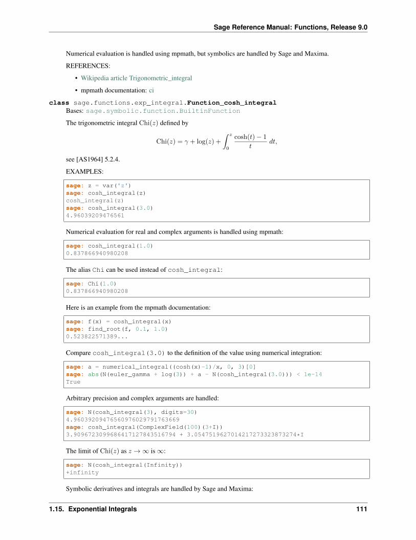
Sage Reference Manual: Functions, Release 9.0
Numerical evaluation is handled using mpmath, but symbolics are handled by Sage and Maxima.
REFERENCES:
• Wikipedia article Trigonometric_integral
• mpmath documentation: ci
class sage.functions.exp_integral.Function_cosh_integralBases: sage.symbolic.function.BuiltinFunction
The trigonometric integral Chi(𝑧) defined by
Chi(𝑧) = 𝛾 + log(𝑧) +
∫ 𝑧
0
cosh(𝑡) − 1
𝑡𝑑𝑡,
see [AS1964] 5.2.4.
EXAMPLES:
sage: z = var('z')sage: cosh_integral(z)cosh_integral(z)sage: cosh_integral(3.0)4.96039209476561
Numerical evaluation for real and complex arguments is handled using mpmath:
sage: cosh_integral(1.0)0.837866940980208
The alias Chi can be used instead of cosh_integral:
sage: Chi(1.0)0.837866940980208
Here is an example from the mpmath documentation:
sage: f(x) = cosh_integral(x)sage: find_root(f, 0.1, 1.0)0.523822571389...
Compare cosh_integral(3.0) to the definition of the value using numerical integration:
sage: a = numerical_integral((cosh(x)-1)/x, 0, 3)[0]sage: abs(N(euler_gamma + log(3)) + a - N(cosh_integral(3.0))) < 1e-14True
Arbitrary precision and complex arguments are handled:
sage: N(cosh_integral(3), digits=30)4.96039209476560976029791763669sage: cosh_integral(ComplexField(100)(3+I))3.9096723099686417127843516794 + 3.0547519627014217273323873274*I
The limit of Chi(𝑧) as 𝑧 → ∞ is ∞:
sage: N(cosh_integral(Infinity))+infinity
Symbolic derivatives and integrals are handled by Sage and Maxima:
1.15. Exponential Integrals 111

Sage Reference Manual: Functions, Release 9.0
sage: x = var('x')sage: f = cosh_integral(x)sage: f.diff(x)cosh(x)/x
sage: f.integrate(x)x*cosh_integral(x) - sinh(x)
ALGORITHM:
Numerical evaluation is handled using mpmath, but symbolics are handled by Sage and Maxima.
REFERENCES:
• Wikipedia article Trigonometric_integral
• mpmath documentation: chi
class sage.functions.exp_integral.Function_exp_integralBases: sage.symbolic.function.BuiltinFunction
The generalized complex exponential integral Ei(z) defined by
Ei(𝑥) =
∫ 𝑥
−∞
𝑒𝑡
𝑡𝑑𝑡
for x > 0 and for complex arguments by analytic continuation, see [AS1964] 5.1.2.
EXAMPLES:
sage: Ei(10)Ei(10)sage: Ei(I)Ei(I)sage: Ei(3+I)Ei(I + 3)sage: Ei(1.3)2.72139888023202sage: Ei(10r)Ei(10)sage: Ei(1.3r)2.7213988802320235
The branch cut for this function is along the negative real axis:
sage: Ei(-3 + 0.1*I)-0.0129379427181693 + 3.13993830250942*Isage: Ei(-3 - 0.1*I)-0.0129379427181693 - 3.13993830250942*I
The precision for the result is deduced from the precision of the input. Convert the input to a higher precisionexplicitly if a result with higher precision is desired:
sage: Ei(RealField(300)(1.1))2.→˓16737827956340282358378734233807621497112737591639704719499002090327541763352339357795426
ALGORITHM: Uses mpmath.
class sage.functions.exp_integral.Function_exp_integral_eBases: sage.symbolic.function.BuiltinFunction
112 Chapter 1. Built-in Functions

Sage Reference Manual: Functions, Release 9.0
The generalized complex exponential integral 𝐸𝑛(𝑧) defined by
𝐸𝑛(𝑧) =
∫ ∞
1
𝑒−𝑧𝑡
𝑡𝑛𝑑𝑡
for complex numbers 𝑛 and 𝑧, see [AS1964] 5.1.4.
The special case where 𝑛 = 1 is denoted in Sage by exp_integral_e1.
EXAMPLES:
Numerical evaluation is handled using mpmath:
sage: N(exp_integral_e(1,1))0.219383934395520sage: exp_integral_e(1, RealField(100)(1))0.21938393439552027367716377546
We can compare this to PARI’s evaluation of exponential_integral_1():
sage: N(exponential_integral_1(1))0.219383934395520
We can verify one case of [AS1964] 5.1.45, i.e. 𝐸𝑛(𝑧) = 𝑧𝑛−1Γ(1 − 𝑛, 𝑧):
sage: N(exp_integral_e(2, 3+I))0.00354575823814662 - 0.00973200528288687*Isage: N((3+I)*gamma(-1, 3+I))0.00354575823814662 - 0.00973200528288687*I
Maxima returns the following improper integral as a multiple of exp_integral_e(1,1):
sage: uu = integral(e^(-x)*log(x+1),x,0,oo)sage: uue*exp_integral_e(1, 1)sage: uu.n(digits=30)0.596347362323194074341078499369
Symbolic derivatives and integrals are handled by Sage and Maxima:
sage: x = var('x')sage: f = exp_integral_e(2,x)sage: f.diff(x)-exp_integral_e(1, x)
sage: f.integrate(x)-exp_integral_e(3, x)
sage: f = exp_integral_e(-1,x)sage: f.integrate(x)Ei(-x) - gamma(-1, x)
Some special values of exp_integral_e can be simplified. [AS1964] 5.1.23:
sage: exp_integral_e(0,x)e^(-x)/x
[AS1964] 5.1.24:
1.15. Exponential Integrals 113

Sage Reference Manual: Functions, Release 9.0
sage: exp_integral_e(6,0)1/5sage: nn = var('nn')sage: assume(nn > 1)sage: f = exp_integral_e(nn,0)sage: f.simplify()1/(nn - 1)
ALGORITHM:
Numerical evaluation is handled using mpmath, but symbolics are handled by Sage and Maxima.
class sage.functions.exp_integral.Function_exp_integral_e1Bases: sage.symbolic.function.BuiltinFunction
The generalized complex exponential integral 𝐸1(𝑧) defined by
𝐸1(𝑧) =
∫ ∞
𝑧
𝑒−𝑡
𝑡𝑑𝑡
see [AS1964] 5.1.4.
EXAMPLES:
sage: exp_integral_e1(x)exp_integral_e1(x)sage: exp_integral_e1(1.0)0.219383934395520
Numerical evaluation is handled using mpmath:
sage: N(exp_integral_e1(1))0.219383934395520sage: exp_integral_e1(RealField(100)(1))0.21938393439552027367716377546
We can compare this to PARI’s evaluation of exponential_integral_1():
sage: N(exp_integral_e1(2.0))0.0489005107080611sage: N(exponential_integral_1(2.0))0.0489005107080611
Symbolic derivatives and integrals are handled by Sage and Maxima:
sage: x = var('x')sage: f = exp_integral_e1(x)sage: f.diff(x)-e^(-x)/x
sage: f.integrate(x)-exp_integral_e(2, x)
ALGORITHM:
Numerical evaluation is handled using mpmath, but symbolics are handled by Sage and Maxima.
class sage.functions.exp_integral.Function_log_integralBases: sage.symbolic.function.BuiltinFunction
114 Chapter 1. Built-in Functions

Sage Reference Manual: Functions, Release 9.0
The logarithmic integral li(𝑧) defined by
li(𝑥) =
∫ 𝑧
0
𝑑𝑡
ln(𝑡)= Ei(ln(𝑥))
for x > 1 and by analytic continuation for complex arguments z (see [AS1964] 5.1.3).
EXAMPLES:
Numerical evaluation for real and complex arguments is handled using mpmath:
sage: N(log_integral(3))2.16358859466719sage: N(log_integral(3), digits=30)2.16358859466719197287692236735sage: log_integral(ComplexField(100)(3+I))2.2879892769816826157078450911 + 0.87232935488528370139883806779*Isage: log_integral(0)0
Symbolic derivatives and integrals are handled by Sage and Maxima:
sage: x = var('x')sage: f = log_integral(x)sage: f.diff(x)1/log(x)
sage: f.integrate(x)x*log_integral(x) - Ei(2*log(x))
Here is a test from the mpmath documentation. There are 1,925,320,391,606,803,968,923 many prime numbersless than 1e23. The value of log_integral(1e23) is very close to this:
sage: log_integral(1e23)1.92532039161405e21
ALGORITHM:
Numerical evaluation is handled using mpmath, but symbolics are handled by Sage and Maxima.
REFERENCES:
• Wikipedia article Logarithmic_integral_function
• mpmath documentation: logarithmic-integral
class sage.functions.exp_integral.Function_log_integral_offsetBases: sage.symbolic.function.BuiltinFunction
The offset logarithmic integral, or Eulerian logarithmic integral, Li(𝑥) is defined by
Li(𝑥) =
∫ 𝑥
2
𝑑𝑡
ln(𝑡)= li(𝑥) − li(2)
for 𝑥 ≥ 2.
The offset logarithmic integral should also not be confused with the polylogarithm (also denoted by Li(𝑥) ),which is implemented as sage.functions.log.Function_polylog.
Li(𝑥) is identical to li(𝑥) except that the lower limit of integration is 2 rather than 0 to avoid the singularity at𝑥 = 1 of
1
ln(𝑡)
1.15. Exponential Integrals 115

Sage Reference Manual: Functions, Release 9.0
See Function_log_integral for details of li(𝑥). Thus Li(𝑥) can also be represented by
Li(𝑥) = li(𝑥) − li(2)
So we have:
sage: li(4.5)-li(2.0)-Li(4.5)0.000000000000000
Li(𝑥) is extended to complex arguments 𝑧 by analytic continuation (see [AS1964] 5.1.3):
sage: Li(6.6+5.4*I)3.97032201503632 + 2.62311237593572*I
The function Li is an approximation for the number of primes up to 𝑥. In fact, the famous Riemann Hypothesisis
|𝜋(𝑥) − Li(𝑥)| ≤√𝑥 log(𝑥).
For “small” 𝑥, Li(𝑥) is always slightly bigger than 𝜋(𝑥). However it is a theorem that there are very large valuesof 𝑥 (e.g., around 10316), such that ∃𝑥 : 𝜋(𝑥) > Li(𝑥). See “A new bound for the smallest x with 𝜋(𝑥) > li(𝑥)”,Bays and Hudson, Mathematics of Computation, 69 (2000) 1285-1296.
Note: Definite integration returns a part symbolic and part numerical result. This is because when Li(x) isevaluated it is passed as li(x)-li(2).
EXAMPLES:
Numerical evaluation for real and complex arguments is handled using mpmath:
sage: N(log_integral_offset(3))1.11842481454970sage: N(log_integral_offset(3), digits=30)1.11842481454969918803233347815sage: log_integral_offset(ComplexField(100)(3+I))1.2428254968641898308632562019 + 0.87232935488528370139883806779*Isage: log_integral_offset(2)0sage: for n in range(1,7):....: print('%-10s%-10s%-20s'%(10^n, prime_pi(10^n), N(Li(10^n))))10 4 5.12043572466980100 25 29.08097780396211000 168 176.56449421003510000 1229 1245.09205211927100000 9592 9628.763837270681000000 78498 78626.5039956821
Here is a test from the mpmath documentation. There are 1,925,320,391,606,803,968,923 prime numbers lessthan 1e23. The value of log_integral_offset(1e23) is very close to this:
sage: log_integral_offset(1e23)1.92532039161405e21
Symbolic derivatives are handled by Sage and integration by Maxima:
116 Chapter 1. Built-in Functions

Sage Reference Manual: Functions, Release 9.0
sage: x = var('x')sage: f = log_integral_offset(x)sage: f.diff(x)1/log(x)sage: f.integrate(x)-x*log_integral(2) + x*log_integral(x) - Ei(2*log(x))sage: Li(x).integrate(x,2.0,4.5)-2.5*log_integral(2) + 5.799321147411334sage: N(f.integrate(x,2.0,3.0)) # abs tol 1e-150.601621785860587
ALGORITHM:
Numerical evaluation is handled using mpmath, but symbolics are handled by Sage and Maxima.
REFERENCES:
• Wikipedia article Logarithmic_integral_function
• mpmath documentation: logarithmic-integral
class sage.functions.exp_integral.Function_sin_integralBases: sage.symbolic.function.BuiltinFunction
The trigonometric integral Si(𝑧) defined by
Si(𝑧) =
∫ 𝑧
0
sin(𝑡)
𝑡𝑑𝑡,
see [AS1964] 5.2.1.
EXAMPLES:
Numerical evaluation for real and complex arguments is handled using mpmath:
sage: sin_integral(0)0sage: sin_integral(0.0)0.000000000000000sage: sin_integral(3.0)1.84865252799947sage: N(sin_integral(3), digits=30)1.84865252799946825639773025111sage: sin_integral(ComplexField(100)(3+I))2.0277151656451253616038525998 + 0.015210926166954211913653130271*I
The alias Si can be used instead of sin_integral:
sage: Si(3.0)1.84865252799947
The limit of Si(𝑧) as 𝑧 → ∞ is 𝜋/2:
sage: N(sin_integral(1e23))1.57079632679490sage: N(pi/2)1.57079632679490
At 200 bits of precision Si(1023) agrees with 𝜋/2 up to 10−24:
1.15. Exponential Integrals 117

Sage Reference Manual: Functions, Release 9.0
sage: sin_integral(RealField(200)(1e23))1.5707963267948966192313288218697837425815368604836679189519sage: N(pi/2, prec=200)1.5707963267948966192313216916397514420985846996875529104875
The exponential sine integral is analytic everywhere:
sage: sin_integral(-1.0)-0.946083070367183sage: sin_integral(-2.0)-1.60541297680269sage: sin_integral(-1e23)-1.57079632679490
Symbolic derivatives and integrals are handled by Sage and Maxima:
sage: x = var('x')sage: f = sin_integral(x)sage: f.diff(x)sin(x)/x
sage: f.integrate(x)x*sin_integral(x) + cos(x)
sage: integrate(sin(x)/x, x)-1/2*I*Ei(I*x) + 1/2*I*Ei(-I*x)
Compare values of the functions Si(𝑥) and 𝑓(𝑥) = (1/2)𝑖 · Ei(−𝑖𝑥) − (1/2)𝑖 · Ei(𝑖𝑥) − 𝜋/2, which are bothanti-derivatives of sin(𝑥)/𝑥, at some random positive real numbers:
sage: f(x) = 1/2*I*Ei(-I*x) - 1/2*I*Ei(I*x) - pi/2sage: g(x) = sin_integral(x)sage: R = [ abs(RDF.random_element()) for i in range(100) ]sage: all(abs(f(x) - g(x)) < 1e-10 for x in R)True
The Nielsen spiral is the parametric plot of (Si(t), Ci(t)):
sage: x=var('x')sage: f(x) = sin_integral(x)sage: g(x) = cos_integral(x)sage: P = parametric_plot([f, g], (x, 0.5 ,20))sage: show(P, frame=True, axes=False)
ALGORITHM:
Numerical evaluation is handled using mpmath, but symbolics are handled by Sage and Maxima.
REFERENCES:
• Wikipedia article Trigonometric_integral
• mpmath documentation: si
class sage.functions.exp_integral.Function_sinh_integralBases: sage.symbolic.function.BuiltinFunction
The trigonometric integral Shi(𝑧) defined by
Shi(𝑧) =
∫ 𝑧
0
sinh(𝑡)
𝑡𝑑𝑡,
118 Chapter 1. Built-in Functions

Sage Reference Manual: Functions, Release 9.0
see [AS1964] 5.2.3.
EXAMPLES:
Numerical evaluation for real and complex arguments is handled using mpmath:
sage: sinh_integral(3.0)4.97344047585981sage: sinh_integral(1.0)1.05725087537573sage: sinh_integral(-1.0)-1.05725087537573
The alias Shi can be used instead of sinh_integral:
sage: Shi(3.0)4.97344047585981
Compare sinh_integral(3.0) to the definition of the value using numerical integration:
sage: a = numerical_integral(sinh(x)/x, 0, 3)[0]sage: abs(a - N(sinh_integral(3))) < 1e-14True
Arbitrary precision and complex arguments are handled:
sage: N(sinh_integral(3), digits=30)4.97344047585980679771041838252sage: sinh_integral(ComplexField(100)(3+I))3.9134623660329374406788354078 + 3.0427678212908839256360163759*I
The limit Shi(𝑧) as 𝑧 → ∞ is ∞:
sage: N(sinh_integral(Infinity))+infinity
Symbolic derivatives and integrals are handled by Sage and Maxima:
sage: x = var('x')sage: f = sinh_integral(x)sage: f.diff(x)sinh(x)/x
sage: f.integrate(x)x*sinh_integral(x) - cosh(x)
Note that due to some problems with the way Maxima handles these expressions, definite integrals can some-times give unexpected results (typically when using inexact endpoints) due to inconsistent branching:
sage: integrate(sinh_integral(x), x, 0, 1/2)-cosh(1/2) + 1/2*sinh_integral(1/2) + 1sage: integrate(sinh_integral(x), x, 0, 1/2).n() # correct0.125872409703453sage: integrate(sinh_integral(x), x, 0, 0.5).n() # fixed in maxima 5.29.10.125872409703453
ALGORITHM:
Numerical evaluation is handled using mpmath, but symbolics are handled by Sage and Maxima.
1.15. Exponential Integrals 119

Sage Reference Manual: Functions, Release 9.0
REFERENCES:
• Wikipedia article Trigonometric_integral
• mpmath documentation: shi
sage.functions.exp_integral.exponential_integral_1(x, n=0)Returns the exponential integral 𝐸1(𝑥). If the optional argument 𝑛 is given, computes list of the first 𝑛 valuesof the exponential integral 𝐸1(𝑥𝑚).
The exponential integral 𝐸1(𝑥) is
𝐸1(𝑥) =
∫ ∞
𝑥
𝑒−𝑡
𝑡𝑑𝑡
INPUT:
• x – a positive real number
• n – (default: 0) a nonnegative integer; if nonzero, then return a list of values E_1(x*m) for m =1,2,3,. . . ,n. This is useful, e.g., when computing derivatives of L-functions.
OUTPUT:
A real number if n is 0 (the default) or a list of reals if n > 0. The precision is the same as the input, with adefault of 53 bits in case the input is exact.
EXAMPLES:
sage: exponential_integral_1(2)0.0489005107080611sage: exponential_integral_1(2, 4) # abs tol 1e-18[0.0489005107080611, 0.00377935240984891, 0.000360082452162659, 0.→˓0000376656228439245]sage: exponential_integral_1(40, 5)[0.000000000000000, 2.22854325868847e-37, 6.33732515501151e-55, 2.02336191509997e-→˓72, 6.88522610630764e-90]sage: exponential_integral_1(0)+Infinitysage: r = exponential_integral_1(RealField(150)(1))sage: r0.21938393439552027367716377546012164903104729sage: parent(r)Real Field with 150 bits of precisionsage: exponential_integral_1(RealField(150)(100))3.6835977616820321802351926205081189876552201e-46
ALGORITHM: use the PARI C-library function eint1.
REFERENCE:
• See Proposition 5.6.12 of Cohen’s book “A Course in Computational Algebraic Number Theory”.
1.16 Wigner, Clebsch-Gordan, Racah, and Gaunt coefficients
Collection of functions for calculating Wigner 3-𝑗, 6-𝑗, 9-𝑗, Clebsch-Gordan, Racah as well as Gaunt coefficientsexactly, all evaluating to a rational number times the square root of a rational number [RH2003].
Please see the description of the individual functions for further details and examples.
AUTHORS:
120 Chapter 1. Built-in Functions

Sage Reference Manual: Functions, Release 9.0
• Jens Rasch (2009-03-24): initial version for Sage
• Jens Rasch (2009-05-31): updated to sage-4.0
sage.functions.wigner.clebsch_gordan(j_1, j_2, j_3, m_1, m_2, m_3, prec=None)Calculates the Clebsch-Gordan coefficient ⟨𝑗1𝑚1 𝑗2𝑚2|𝑗3𝑚3⟩.
The reference for this function is [Ed1974].
INPUT:
• j_1, j_2, j_3, m_1, m_2, m_3 - integer or half integer
• prec - precision, default: None. Providing a precision can drastically speed up the calculation.
OUTPUT:
Rational number times the square root of a rational number (if prec=None), or real number if a precision isgiven.
EXAMPLES:
sage: simplify(clebsch_gordan(3/2,1/2,2, 3/2,1/2,2))1sage: clebsch_gordan(1.5,0.5,1, 1.5,-0.5,1)1/2*sqrt(3)sage: clebsch_gordan(3/2,1/2,1, -1/2,1/2,0)-sqrt(3)*sqrt(1/6)
NOTES:
The Clebsch-Gordan coefficient will be evaluated via its relation to Wigner 3-𝑗 symbols:
⟨𝑗1𝑚1 𝑗2𝑚2|𝑗3𝑚3⟩ = (−1)𝑗1−𝑗2+𝑚3√
2𝑗3 + 1
(𝑗1 𝑗2 𝑗3𝑚1 𝑚2 −𝑚3
)See also the documentation on Wigner 3-𝑗 symbols which exhibit much higher symmetry relations than theClebsch-Gordan coefficient.
AUTHORS:
• Jens Rasch (2009-03-24): initial version
sage.functions.wigner.gaunt(l_1, l_2, l_3, m_1, m_2, m_3, prec=None)Calculate the Gaunt coefficient.
The Gaunt coefficient is defined as the integral over three spherical harmonics:
𝑌 (𝑙1, 𝑙2, 𝑙3,𝑚1,𝑚2,𝑚3)
=
∫𝑌𝑙1,𝑚1
(Ω) 𝑌𝑙2,𝑚2(Ω) 𝑌𝑙3,𝑚3
(Ω) 𝑑Ω
=
√(2𝑙1 + 1)(2𝑙2 + 1)(2𝑙3 + 1)
4𝜋
×(𝑙1 𝑙2 𝑙30 0 0
)(𝑙1 𝑙2 𝑙3𝑚1 𝑚2 𝑚3
)INPUT:
• l_1, l_2, l_3, m_1, m_2, m_3 - integer
• prec - precision, default: None. Providing a precision can drastically speed up the calculation.
1.16. Wigner, Clebsch-Gordan, Racah, and Gaunt coefficients 121

Sage Reference Manual: Functions, Release 9.0
OUTPUT:
Rational number times the square root of a rational number (if prec=None), or real number if a precision isgiven.
EXAMPLES:
sage: gaunt(1,0,1,1,0,-1)-1/2/sqrt(pi)sage: gaunt(1,0,1,1,0,0)0sage: gaunt(29,29,34,10,-5,-5)1821867940156/215552371055153321*sqrt(22134)/sqrt(pi)sage: gaunt(20,20,40,1,-1,0)28384503878959800/74029560764440771/sqrt(pi)sage: gaunt(12,15,5,2,3,-5)91/124062*sqrt(36890)/sqrt(pi)sage: gaunt(10,10,12,9,3,-12)-98/62031*sqrt(6279)/sqrt(pi)sage: gaunt(1000,1000,1200,9,3,-12).n(64)0.00689500421922113448
If the sum of the 𝑙𝑖 is odd, the answer is zero, even for Python ints (see trac ticket #14766):
sage: gaunt(1,2,2,1,0,-1)0sage: gaunt(int(1),int(2),int(2),1,0,-1)0
It is an error to use non-integer values for 𝑙 or 𝑚:
sage: gaunt(1.2,0,1.2,0,0,0)Traceback (most recent call last):...TypeError: Attempt to coerce non-integral RealNumber to Integersage: gaunt(1,0,1,1.1,0,-1.1)Traceback (most recent call last):...TypeError: Attempt to coerce non-integral RealNumber to Integer
NOTES:
The Gaunt coefficient obeys the following symmetry rules:
• invariant under any permutation of the columns
𝑌 (𝑙1, 𝑙2, 𝑙3,𝑚1,𝑚2,𝑚3) = 𝑌 (𝑙3, 𝑙1, 𝑙2,𝑚3,𝑚1,𝑚2)
= 𝑌 (𝑙2, 𝑙3, 𝑙1,𝑚2,𝑚3,𝑚1) = 𝑌 (𝑙3, 𝑙2, 𝑙1,𝑚3,𝑚2,𝑚1)
= 𝑌 (𝑙1, 𝑙3, 𝑙2,𝑚1,𝑚3,𝑚2) = 𝑌 (𝑙2, 𝑙1, 𝑙3,𝑚2,𝑚1,𝑚3)
• invariant under space inflection, i.e.
𝑌 (𝑙1, 𝑙2, 𝑙3,𝑚1,𝑚2,𝑚3) = 𝑌 (𝑙1, 𝑙2, 𝑙3,−𝑚1,−𝑚2,−𝑚3)
• symmetric with respect to the 72 Regge symmetries as inherited for the 3-𝑗 symbols [Reg1958]
• zero for 𝑙1, 𝑙2, 𝑙3 not fulfilling triangle relation
• zero for violating any one of the conditions: 𝑙1 ≥ |𝑚1|, 𝑙2 ≥ |𝑚2|, 𝑙3 ≥ |𝑚3|
122 Chapter 1. Built-in Functions

Sage Reference Manual: Functions, Release 9.0
• non-zero only for an even sum of the 𝑙𝑖, i.e. 𝐽 = 𝑙1 + 𝑙2 + 𝑙3 = 2𝑛 for 𝑛 in N
ALGORITHM:
This function uses the algorithm of [LdB1982] to calculate the value of the Gaunt coefficient exactly. Notethat the formula contains alternating sums over large factorials and is therefore unsuitable for finite precisionarithmetic and only useful for a computer algebra system [RH2003].
AUTHORS:
• Jens Rasch (2009-03-24): initial version for Sage
sage.functions.wigner.racah(aa, bb, cc, dd, ee, ff, prec=None)Calculate the Racah symbol 𝑊 (𝑎𝑎, 𝑏𝑏, 𝑐𝑐, 𝑑𝑑; 𝑒𝑒, 𝑓𝑓).
INPUT:
• aa, . . . , ff - integer or half integer
• prec - precision, default: None. Providing a precision can drastically speed up the calculation.
OUTPUT:
Rational number times the square root of a rational number (if prec=None), or real number if a precision isgiven.
EXAMPLES:
sage: racah(3,3,3,3,3,3)-1/14
NOTES:
The Racah symbol is related to the Wigner 6-𝑗 symbol:𝑗1 𝑗2 𝑗3𝑗4 𝑗5 𝑗6
= (−1)𝑗1+𝑗2+𝑗4+𝑗5𝑊 (𝑗1, 𝑗2, 𝑗5, 𝑗4; 𝑗3, 𝑗6)
Please see the 6-𝑗 symbol for its much richer symmetries and for additional properties.
ALGORITHM:
This function uses the algorithm of [Ed1974] to calculate the value of the 6-𝑗 symbol exactly. Note that theformula contains alternating sums over large factorials and is therefore unsuitable for finite precision arithmeticand only useful for a computer algebra system [RH2003].
AUTHORS:
• Jens Rasch (2009-03-24): initial version
sage.functions.wigner.wigner_3j(j_1, j_2, j_3, m_1, m_2, m_3, prec=None)
Calculate the Wigner 3-𝑗 symbol(𝑗1 𝑗2 𝑗3𝑚1 𝑚2 𝑚3
).
INPUT:
• j_1, j_2, j_3, m_1, m_2, m_3 - integer or half integer
• prec - precision, default: None. Providing a precision can drastically speed up the calculation.
OUTPUT:
Rational number times the square root of a rational number (if prec=None), or real number if a precision isgiven.
EXAMPLES:
1.16. Wigner, Clebsch-Gordan, Racah, and Gaunt coefficients 123
Sage Reference Manual: Functions, Release 9.0
sage: wigner_3j(2, 6, 4, 0, 0, 0)sqrt(5/143)sage: wigner_3j(2, 6, 4, 0, 0, 1)0sage: wigner_3j(0.5, 0.5, 1, 0.5, -0.5, 0)sqrt(1/6)sage: wigner_3j(40, 100, 60, -10, 60, -50)95608/18702538494885*sqrt(21082735836735314343364163310/220491455010479533763)sage: wigner_3j(2500, 2500, 5000, 2488, 2400, -4888, prec=64)7.60424456883448589e-12
It is an error to have arguments that are not integer or half integer values:
sage: wigner_3j(2.1, 6, 4, 0, 0, 0)Traceback (most recent call last):...ValueError: j values must be integer or half integersage: wigner_3j(2, 6, 4, 1, 0, -1.1)Traceback (most recent call last):...ValueError: m values must be integer or half integer
NOTES:
The Wigner 3-𝑗 symbol obeys the following symmetry rules:
• invariant under any permutation of the columns (with the exception of a sign change where 𝐽 = 𝑗1 + 𝑗2 +𝑗3): (
𝑗1 𝑗2 𝑗3𝑚1 𝑚2 𝑚3
)=
(𝑗3 𝑗1 𝑗2𝑚3 𝑚1 𝑚2
)=
(𝑗2 𝑗3 𝑗1𝑚2 𝑚3 𝑚1
)= (−1)𝐽
(𝑗3 𝑗2 𝑗1𝑚3 𝑚2 𝑚1
)= (−1)𝐽
(𝑗1 𝑗3 𝑗2𝑚1 𝑚3 𝑚2
)= (−1)𝐽
(𝑗2 𝑗1 𝑗3𝑚2 𝑚1 𝑚3
)• invariant under space inflection, i.e.(
𝑗1 𝑗2 𝑗3𝑚1 𝑚2 𝑚3
)= (−1)𝐽
(𝑗1 𝑗2 𝑗3
−𝑚1 −𝑚2 −𝑚3
)• symmetric with respect to the 72 additional symmetries based on the work by [Reg1958]
• zero for 𝑗1, 𝑗2, 𝑗3 not fulfilling triangle relation
• zero for 𝑚1 + 𝑚2 + 𝑚3 = 0
• zero for violating any one of the conditions 𝑗1 ≥ |𝑚1|, 𝑗2 ≥ |𝑚2|, 𝑗3 ≥ |𝑚3|
ALGORITHM:
This function uses the algorithm of [Ed1974] to calculate the value of the 3-𝑗 symbol exactly. Note that theformula contains alternating sums over large factorials and is therefore unsuitable for finite precision arithmeticand only useful for a computer algebra system [RH2003].
AUTHORS:
• Jens Rasch (2009-03-24): initial version
sage.functions.wigner.wigner_6j(j_1, j_2, j_3, j_4, j_5, j_6, prec=None)
Calculate the Wigner 6-𝑗 symbol𝑗1 𝑗2 𝑗3𝑗4 𝑗5 𝑗6
.
INPUT:
124 Chapter 1. Built-in Functions

Sage Reference Manual: Functions, Release 9.0
• j_1, . . . , j_6 - integer or half integer
• prec - precision, default: None. Providing a precision can drastically speed up the calculation.
OUTPUT:
Rational number times the square root of a rational number (if prec=None), or real number if a precision isgiven.
EXAMPLES:
sage: wigner_6j(3,3,3,3,3,3)-1/14sage: wigner_6j(5,5,5,5,5,5)1/52sage: wigner_6j(6,6,6,6,6,6)309/10868sage: wigner_6j(8,8,8,8,8,8)-12219/965770sage: wigner_6j(30,30,30,30,30,30)36082186869033479581/87954851694828981714124sage: wigner_6j(0.5,0.5,1,0.5,0.5,1)1/6sage: wigner_6j(200,200,200,200,200,200, prec=1000)*1.00.000155903212413242
It is an error to have arguments that are not integer or half integer values or do not fulfill the triangle relation:
sage: wigner_6j(2.5,2.5,2.5,2.5,2.5,2.5)Traceback (most recent call last):...ValueError: j values must be integer or half integer and fulfill the triangle→˓relationsage: wigner_6j(0.5,0.5,1.1,0.5,0.5,1.1)Traceback (most recent call last):...ValueError: j values must be integer or half integer and fulfill the triangle→˓relation
NOTES:
The Wigner 6-𝑗 symbol is related to the Racah symbol but exhibits more symmetries as detailed below.𝑗1 𝑗2 𝑗3𝑗4 𝑗5 𝑗6
= (−1)𝑗1+𝑗2+𝑗4+𝑗5𝑊 (𝑗1, 𝑗2, 𝑗5, 𝑗4; 𝑗3, 𝑗6)
The Wigner 6-𝑗 symbol obeys the following symmetry rules:
• Wigner 6-𝑗 symbols are left invariant under any permutation of the columns:𝑗1 𝑗2 𝑗3𝑗4 𝑗5 𝑗6
=
𝑗3 𝑗1 𝑗2𝑗6 𝑗4 𝑗5
=
𝑗2 𝑗3 𝑗1𝑗5 𝑗6 𝑗4
=
𝑗3 𝑗2 𝑗1𝑗6 𝑗5 𝑗4
=
𝑗1 𝑗3 𝑗2𝑗4 𝑗6 𝑗5
=
𝑗2 𝑗1 𝑗3𝑗5 𝑗4 𝑗6
• They are invariant under the exchange of the upper and lower arguments in each of any two columns, i.e.𝑗1 𝑗2 𝑗3𝑗4 𝑗5 𝑗6
=
𝑗1 𝑗5 𝑗6𝑗4 𝑗2 𝑗3
=
𝑗4 𝑗2 𝑗6𝑗1 𝑗5 𝑗3
=
𝑗4 𝑗5 𝑗3𝑗1 𝑗2 𝑗6
1.16. Wigner, Clebsch-Gordan, Racah, and Gaunt coefficients 125

Sage Reference Manual: Functions, Release 9.0
• additional 6 symmetries [Reg1959] giving rise to 144 symmetries in total
• only non-zero if any triple of 𝑗’s fulfill a triangle relation
ALGORITHM:
This function uses the algorithm of [Ed1974] to calculate the value of the 6-𝑗 symbol exactly. Note that theformula contains alternating sums over large factorials and is therefore unsuitable for finite precision arithmeticand only useful for a computer algebra system [RH2003].
sage.functions.wigner.wigner_9j(j_1, j_2, j_3, j_4, j_5, j_6, j_7, j_8, j_9, prec=None)
Calculate the Wigner 9-𝑗 symbol
⎧⎨⎩𝑗1 𝑗2 𝑗3𝑗4 𝑗5 𝑗6𝑗7 𝑗8 𝑗9
⎫⎬⎭.
INPUT:
• j_1, . . . , j_9 - integer or half integer
• prec - precision, default: None. Providing a precision can drastically speed up the calculation.
OUTPUT:
Rational number times the square root of a rational number (if prec=None), or real number if a precision isgiven.
EXAMPLES:
A couple of examples and test cases, note that for speed reasons a precision is given:
sage: wigner_9j(1,1,1, 1,1,1, 1,1,0 ,prec=64) # ==1/180.0555555555555555555sage: wigner_9j(1,1,1, 1,1,1, 1,1,1)0sage: wigner_9j(1,1,1, 1,1,1, 1,1,2 ,prec=64) # ==1/180.0555555555555555556sage: wigner_9j(1,2,1, 2,2,2, 1,2,1 ,prec=64) # ==-1/150-0.00666666666666666667sage: wigner_9j(3,3,2, 2,2,2, 3,3,2 ,prec=64) # ==157/147000.0106802721088435374sage: wigner_9j(3,3,2, 3,3,2, 3,3,2 ,prec=64) # ==3221*sqrt(70)/→˓(246960*sqrt(105)) - 365/(3528*sqrt(70)*sqrt(105))0.00944247746651111739sage: wigner_9j(3,3,1, 3.5,3.5,2, 3.5,3.5,1 ,prec=64) # ==3221*sqrt(70)/→˓(246960*sqrt(105)) - 365/(3528*sqrt(70)*sqrt(105))0.0110216678544351364sage: wigner_9j(100,80,50, 50,100,70, 60,50,100 ,prec=1000)*1.01.05597798065761e-7sage: wigner_9j(30,30,10, 30.5,30.5,20, 30.5,30.5,10 ,prec=1000)*1.0 #→˓==(80944680186359968990/95103769817469)*sqrt(1/682288158959699477295)0.0000325841699408828sage: wigner_9j(64,62.5,114.5, 61.5,61,112.5, 113.5,110.5,60, prec=1000)*1.0-3.41407910055520e-39sage: wigner_9j(15,15,15, 15,3,15, 15,18,10, prec=1000)*1.0-0.0000778324615309539sage: wigner_9j(1.5,1,1.5, 1,1,1, 1.5,1,1.5)0
It is an error to have arguments that are not integer or half integer values or do not fulfill the triangle relation:
126 Chapter 1. Built-in Functions

Sage Reference Manual: Functions, Release 9.0
sage: wigner_9j(0.5,0.5,0.5, 0.5,0.5,0.5, 0.5,0.5,0.5,prec=64)Traceback (most recent call last):...ValueError: j values must be integer or half integer and fulfill the triangle→˓relationsage: wigner_9j(1,1,1, 0.5,1,1.5, 0.5,1,2.5,prec=64)Traceback (most recent call last):...ValueError: j values must be integer or half integer and fulfill the triangle→˓relation
ALGORITHM:
This function uses the algorithm of [Ed1974] to calculate the value of the 3-𝑗 symbol exactly. Note that theformula contains alternating sums over large factorials and is therefore unsuitable for finite precision arithmeticand only useful for a computer algebra system [RH2003].
1.17 Generalized Functions
Sage implements several generalized functions (also known as distributions) such as Dirac delta, Heaviside step func-tions. These generalized functions can be manipulated within Sage like any other symbolic functions.
AUTHORS:
• Golam Mortuza Hossain (2009-06-26): initial version
EXAMPLES:
Dirac delta function:
sage: dirac_delta(x)dirac_delta(x)
Heaviside step function:
sage: heaviside(x)heaviside(x)
Unit step function:
sage: unit_step(x)unit_step(x)
Signum (sgn) function:
sage: sgn(x)sgn(x)
Kronecker delta function:
sage: m,n=var('m,n')sage: kronecker_delta(m,n)kronecker_delta(m, n)
class sage.functions.generalized.FunctionDiracDeltaBases: sage.symbolic.function.BuiltinFunction
The Dirac delta (generalized) function, 𝛿(𝑥) (dirac_delta(x)).
1.17. Generalized Functions 127
Sage Reference Manual: Functions, Release 9.0
INPUT:
• x - a real number or a symbolic expression
DEFINITION:
Dirac delta function 𝛿(𝑥), is defined in Sage as:
𝛿(𝑥) = 0 for real 𝑥 = 0 and∫∞−∞ 𝛿(𝑥)𝑑𝑥 = 1
Its alternate definition with respect to an arbitrary test function 𝑓(𝑥) is∫∞−∞ 𝑓(𝑥)𝛿(𝑥− 𝑎)𝑑𝑥 = 𝑓(𝑎)
EXAMPLES:
sage: dirac_delta(1)0sage: dirac_delta(0)dirac_delta(0)sage: dirac_delta(x)dirac_delta(x)sage: integrate(dirac_delta(x), x, -1, 1, algorithm='sympy')1
REFERENCES:
• Wikipedia article Dirac_delta_function
class sage.functions.generalized.FunctionHeavisideBases: sage.symbolic.function.GinacFunction
The Heaviside step function, 𝐻(𝑥) (heaviside(x)).
INPUT:
• x - a real number or a symbolic expression
DEFINITION:
The Heaviside step function, 𝐻(𝑥) is defined in Sage as:
𝐻(𝑥) = 0 for 𝑥 < 0 and 𝐻(𝑥) = 1 for 𝑥 > 0
See also:
unit_step()
EXAMPLES:
sage: heaviside(-1)0sage: heaviside(1)1sage: heaviside(0)heaviside(0)sage: heaviside(x)heaviside(x)
sage: heaviside(-1/2)0sage: heaviside(exp(-1000000000000000000000))1
REFERENCES:
128 Chapter 1. Built-in Functions

Sage Reference Manual: Functions, Release 9.0
• Wikipedia article Heaviside_function
class sage.functions.generalized.FunctionKroneckerDeltaBases: sage.symbolic.function.BuiltinFunction
The Kronecker delta function 𝛿𝑚,𝑛 (kronecker_delta(m, n)).
INPUT:
• m - a number or a symbolic expression
• n - a number or a symbolic expression
DEFINITION:
Kronecker delta function 𝛿𝑚,𝑛 is defined as:
𝛿𝑚,𝑛 = 0 for 𝑚 = 𝑛 and 𝛿𝑚,𝑛 = 1 for 𝑚 = 𝑛
EXAMPLES:
sage: kronecker_delta(1,2)0sage: kronecker_delta(1,1)1sage: m,n=var('m,n')sage: kronecker_delta(m,n)kronecker_delta(m, n)
REFERENCES:
• Wikipedia article Kronecker_delta
class sage.functions.generalized.FunctionSignumBases: sage.symbolic.function.BuiltinFunction
The signum or sgn function sgn(𝑥) (sgn(x)).
INPUT:
• x - a real number or a symbolic expression
DEFINITION:
The sgn function, sgn(𝑥) is defined as:
sgn(𝑥) = 1 for 𝑥 > 0, sgn(𝑥) = 0 for 𝑥 = 0 and sgn(𝑥) = −1 for 𝑥 < 0
EXAMPLES:
sage: sgn(-1)-1sage: sgn(1)1sage: sgn(0)0sage: sgn(x)sgn(x)
We can also use sign:
sage: sign(1)1sage: sign(0)
(continues on next page)
1.17. Generalized Functions 129

Sage Reference Manual: Functions, Release 9.0
(continued from previous page)
0sage: a = AA(-5).nth_root(7)sage: sign(a)-1
REFERENCES:
• Wikipedia article Sign_function
class sage.functions.generalized.FunctionUnitStepBases: sage.symbolic.function.GinacFunction
The unit step function, u(𝑥) (unit_step(x)).
INPUT:
• x - a real number or a symbolic expression
DEFINITION:
The unit step function, u(𝑥) is defined in Sage as:
u(𝑥) = 0 for 𝑥 < 0 and u(𝑥) = 1 for 𝑥 ≥ 0
See also:
heaviside()
EXAMPLES:
sage: unit_step(-1)0sage: unit_step(1)1sage: unit_step(0)1sage: unit_step(x)unit_step(x)sage: unit_step(-exp(-10000000000000000000))0
1.18 Counting Primes
AUTHORS:
• R. Andrew Ohana (2009): initial version of efficient prime_pi
• William Stein (2009): fix plot method
• R. Andrew Ohana (2011): complete rewrite, ~5x speedup
EXAMPLES:
sage: z = sage.functions.prime_pi.PrimePi()sage: loads(dumps(z))prime_pisage: loads(dumps(z)) == zTrue
130 Chapter 1. Built-in Functions
Sage Reference Manual: Functions, Release 9.0
class sage.functions.prime_pi.PrimePiBases: sage.symbolic.function.BuiltinFunction
The prime counting function, which counts the number of primes less than or equal to a given value.
INPUT:
• x - a real number
• prime_bound - (default 0) a real number < 2^32, prime_pi will make sure to use all the primes upto prime_bound (although, possibly more) in computing prime_pi, this can potentially speedup thetime of computation, at a cost to memory usage.
OUTPUT:
integer – the number of primes ≤ x
EXAMPLES:
These examples test common inputs:
sage: prime_pi(7)4sage: prime_pi(100)25sage: prime_pi(1000)168sage: prime_pi(100000)9592sage: prime_pi(500509)41581
These examples test a variety of odd inputs:
sage: prime_pi(3.5)2sage: prime_pi(sqrt(2357))15sage: prime_pi(mod(30957, 9750979))Traceback (most recent call last):...TypeError: cannot coerce arguments: positive characteristic not allowed in→˓symbolic computations
We test non-trivial prime_bound values:
sage: prime_pi(100000, 10000)9592sage: prime_pi(500509, 50051)41581
The following test is to verify that trac ticket #4670 has been essentially resolved:
sage: prime_pi(10^10)455052511
The prime_pi function also has a special plotting method, so it plots quickly and perfectly as a step function:
sage: P = plot(prime_pi, 50, 100)
NOTES:
1.18. Counting Primes 131
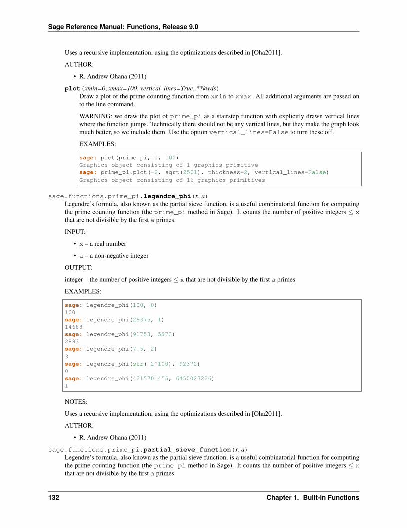
Sage Reference Manual: Functions, Release 9.0
Uses a recursive implementation, using the optimizations described in [Oha2011].
AUTHOR:
• R. Andrew Ohana (2011)
plot(xmin=0, xmax=100, vertical_lines=True, **kwds)Draw a plot of the prime counting function from xmin to xmax. All additional arguments are passed onto the line command.
WARNING: we draw the plot of prime_pi as a stairstep function with explicitly drawn vertical lineswhere the function jumps. Technically there should not be any vertical lines, but they make the graph lookmuch better, so we include them. Use the option vertical_lines=False to turn these off.
EXAMPLES:
sage: plot(prime_pi, 1, 100)Graphics object consisting of 1 graphics primitivesage: prime_pi.plot(-2, sqrt(2501), thickness=2, vertical_lines=False)Graphics object consisting of 16 graphics primitives
sage.functions.prime_pi.legendre_phi(x, a)Legendre’s formula, also known as the partial sieve function, is a useful combinatorial function for computingthe prime counting function (the prime_pi method in Sage). It counts the number of positive integers ≤ xthat are not divisible by the first a primes.
INPUT:
• x – a real number
• a – a non-negative integer
OUTPUT:
integer – the number of positive integers ≤ x that are not divisible by the first a primes
EXAMPLES:
sage: legendre_phi(100, 0)100sage: legendre_phi(29375, 1)14688sage: legendre_phi(91753, 5973)2893sage: legendre_phi(7.5, 2)3sage: legendre_phi(str(-2^100), 92372)0sage: legendre_phi(4215701455, 6450023226)1
NOTES:
Uses a recursive implementation, using the optimizations described in [Oha2011].
AUTHOR:
• R. Andrew Ohana (2011)
sage.functions.prime_pi.partial_sieve_function(x, a)Legendre’s formula, also known as the partial sieve function, is a useful combinatorial function for computingthe prime counting function (the prime_pi method in Sage). It counts the number of positive integers ≤ xthat are not divisible by the first a primes.
132 Chapter 1. Built-in Functions

Sage Reference Manual: Functions, Release 9.0
INPUT:
• x – a real number
• a – a non-negative integer
OUTPUT:
integer – the number of positive integers ≤ x that are not divisible by the first a primes
EXAMPLES:
sage: legendre_phi(100, 0)100sage: legendre_phi(29375, 1)14688sage: legendre_phi(91753, 5973)2893sage: legendre_phi(7.5, 2)3sage: legendre_phi(str(-2^100), 92372)0sage: legendre_phi(4215701455, 6450023226)1
NOTES:
Uses a recursive implementation, using the optimizations described in [Oha2011].
AUTHOR:
• R. Andrew Ohana (2011)
1.19 Symbolic Minimum and Maximum
Sage provides a symbolic maximum and minimum due to the fact that the Python builtin max and min are not able todeal with variables as users might expect. These functions wait to evaluate if there are variables.
Here you can see some differences:
sage: max(x,x^2)xsage: max_symbolic(x,x^2)max(x, x^2)sage: f(x) = max_symbolic(x,x^2); f(1/2)1/2
This works as expected for more than two entries:
sage: max(3,5,x)5sage: min(3,5,x)3sage: max_symbolic(3,5,x)max(x, 5)sage: min_symbolic(3,5,x)min(x, 3)
class sage.functions.min_max.MaxSymbolicBases: sage.functions.min_max.MinMax_base
1.19. Symbolic Minimum and Maximum 133

Sage Reference Manual: Functions, Release 9.0
Symbolic max function.
The Python builtin max function doesn’t work as expected when symbolic expressions are given as arguments.This function delays evaluation until all symbolic arguments are substituted with values.
EXAMPLES:
sage: max_symbolic(3, x)max(3, x)sage: max_symbolic(3, x).subs(x=5)5sage: max_symbolic(3, 5, x)max(x, 5)sage: max_symbolic([3,5,x])max(x, 5)
class sage.functions.min_max.MinMax_baseBases: sage.symbolic.function.BuiltinFunction
eval_helper(this_f, builtin_f, initial_val, args)EXAMPLES:
sage: max_symbolic(3,5,x) # indirect doctestmax(x, 5)sage: min_symbolic(3,5,x)min(x, 3)
class sage.functions.min_max.MinSymbolicBases: sage.functions.min_max.MinMax_base
Symbolic min function.
The Python builtin min function doesn’t work as expected when symbolic expressions are given as arguments.This function delays evaluation until all symbolic arguments are substituted with values.
EXAMPLES:
sage: min_symbolic(3, x)min(3, x)sage: min_symbolic(3, x).subs(x=5)3sage: min_symbolic(3, 5, x)min(x, 3)sage: min_symbolic([3,5,x])min(x, 3)
Please find extensive developer documentation for creating new functions in Symbolic Calculus, in particular in thesection Classes for symbolic functions.
134 Chapter 1. Built-in Functions

CHAPTER
TWO
INDICES AND TABLES
• Index
• Module Index
• Search Page
135

Sage Reference Manual: Functions, Release 9.0
136 Chapter 2. Indices and Tables

PYTHON MODULE INDEX
fsage.functions.airy, 89sage.functions.bessel, 94sage.functions.error, 33sage.functions.exp_integral, 109sage.functions.generalized, 127sage.functions.hyperbolic, 20sage.functions.hypergeometric, 77sage.functions.jacobi, 86sage.functions.log, 1sage.functions.min_max, 133sage.functions.orthogonal_polys, 49sage.functions.other, 60sage.functions.piecewise, 36sage.functions.prime_pi, 130sage.functions.special, 72sage.functions.spike_function, 47sage.functions.transcendental, 28sage.functions.trig, 10sage.functions.wigner, 120
137

Sage Reference Manual: Functions, Release 9.0
138 Python Module Index

INDEX
Aairy_ai() (in module sage.functions.airy), 91airy_bi() (in module sage.functions.airy), 93approximate() (sage.functions.transcendental.DickmanRho method), 29
BBessel() (in module sage.functions.bessel), 97
CChebyshevFunction (class in sage.functions.orthogonal_polys), 52clebsch_gordan() (in module sage.functions.wigner), 121closed_form() (in module sage.functions.hypergeometric), 85convolution() (sage.functions.piecewise.PiecewiseFunction.EvaluationMethods method), 37critical_points() (sage.functions.piecewise.PiecewiseFunction.EvaluationMethods method), 37
Ddeflated() (sage.functions.hypergeometric.Hypergeometric.EvaluationMethods method), 80DickmanRho (class in sage.functions.transcendental), 28domain() (sage.functions.piecewise.PiecewiseFunction.EvaluationMethods method), 37domains() (sage.functions.piecewise.PiecewiseFunction.EvaluationMethods method), 38
Eeliminate_parameters() (sage.functions.hypergeometric.Hypergeometric.EvaluationMethods method), 81elliptic_eu_f() (in module sage.functions.special), 76elliptic_j() (in module sage.functions.special), 77EllipticE (class in sage.functions.special), 73EllipticEC (class in sage.functions.special), 74EllipticEU (class in sage.functions.special), 74EllipticF (class in sage.functions.special), 75EllipticKC (class in sage.functions.special), 75EllipticPi (class in sage.functions.special), 76end_points() (sage.functions.piecewise.PiecewiseFunction.EvaluationMethods method), 38eval_algebraic() (sage.functions.orthogonal_polys.Func_chebyshev_T method), 53eval_algebraic() (sage.functions.orthogonal_polys.Func_chebyshev_U method), 54eval_formula() (sage.functions.orthogonal_polys.Func_chebyshev_T method), 53eval_formula() (sage.functions.orthogonal_polys.Func_chebyshev_U method), 55eval_formula() (sage.functions.orthogonal_polys.Func_legendre_Q method), 58
139

Sage Reference Manual: Functions, Release 9.0
eval_formula() (sage.functions.orthogonal_polys.OrthogonalFunction method), 60eval_helper() (sage.functions.min_max.MinMax_base method), 134eval_poly() (sage.functions.orthogonal_polys.Func_assoc_legendre_P method), 52eval_recursive() (sage.functions.orthogonal_polys.Func_assoc_legendre_Q method), 52eval_recursive() (sage.functions.orthogonal_polys.Func_legendre_Q method), 58exponential_integral_1() (in module sage.functions.exp_integral), 120expression_at() (sage.functions.piecewise.PiecewiseFunction.EvaluationMethods method), 38expressions() (sage.functions.piecewise.PiecewiseFunction.EvaluationMethods method), 39extension() (sage.functions.piecewise.PiecewiseFunction.EvaluationMethods method), 39
Ffourier_series_cosine_coefficient() (sage.functions.piecewise.PiecewiseFunction.EvaluationMethods
method), 39fourier_series_partial_sum() (sage.functions.piecewise.PiecewiseFunction.EvaluationMethods method),
40fourier_series_sine_coefficient() (sage.functions.piecewise.PiecewiseFunction.EvaluationMethods
method), 41Func_assoc_legendre_P (class in sage.functions.orthogonal_polys), 52Func_assoc_legendre_Q (class in sage.functions.orthogonal_polys), 52Func_chebyshev_T (class in sage.functions.orthogonal_polys), 53Func_chebyshev_U (class in sage.functions.orthogonal_polys), 54Func_gen_laguerre (class in sage.functions.orthogonal_polys), 55Func_hermite (class in sage.functions.orthogonal_polys), 55Func_jacobi_P (class in sage.functions.orthogonal_polys), 56Func_laguerre (class in sage.functions.orthogonal_polys), 57Func_legendre_P (class in sage.functions.orthogonal_polys), 57Func_legendre_Q (class in sage.functions.orthogonal_polys), 58Func_ultraspherical (class in sage.functions.orthogonal_polys), 58Function_abs (class in sage.functions.other), 61Function_arccos (class in sage.functions.trig), 10Function_arccosh (class in sage.functions.hyperbolic), 20Function_arccot (class in sage.functions.trig), 11Function_arccoth (class in sage.functions.hyperbolic), 21Function_arccsc (class in sage.functions.trig), 11Function_arccsch (class in sage.functions.hyperbolic), 22Function_arcsec (class in sage.functions.trig), 12Function_arcsech (class in sage.functions.hyperbolic), 22Function_arcsin (class in sage.functions.trig), 13Function_arcsinh (class in sage.functions.hyperbolic), 23Function_arctan (class in sage.functions.trig), 13Function_arctan2 (class in sage.functions.trig), 14Function_arctanh (class in sage.functions.hyperbolic), 23Function_arg (class in sage.functions.other), 61Function_Bessel_I (class in sage.functions.bessel), 99Function_Bessel_J (class in sage.functions.bessel), 101Function_Bessel_K (class in sage.functions.bessel), 102Function_Bessel_Y (class in sage.functions.bessel), 103Function_binomial (class in sage.functions.other), 62Function_cases (class in sage.functions.other), 63Function_ceil (class in sage.functions.other), 64
140 Index
Sage Reference Manual: Functions, Release 9.0
Function_conjugate (class in sage.functions.other), 65Function_cos (class in sage.functions.trig), 15Function_cos_integral (class in sage.functions.exp_integral), 109Function_cosh (class in sage.functions.hyperbolic), 24Function_cosh_integral (class in sage.functions.exp_integral), 111Function_cot (class in sage.functions.trig), 16Function_coth (class in sage.functions.hyperbolic), 25Function_crootof (class in sage.functions.other), 65Function_csc (class in sage.functions.trig), 17Function_csch (class in sage.functions.hyperbolic), 25Function_dilog (class in sage.functions.log), 1Function_erf (class in sage.functions.error), 34Function_erfc (class in sage.functions.error), 35Function_erfi (class in sage.functions.error), 35Function_erfinv (class in sage.functions.error), 35Function_exp (class in sage.functions.log), 2Function_exp_integral (class in sage.functions.exp_integral), 112Function_exp_integral_e (class in sage.functions.exp_integral), 112Function_exp_integral_e1 (class in sage.functions.exp_integral), 114Function_exp_polar (class in sage.functions.log), 3Function_factorial (class in sage.functions.other), 66Function_floor (class in sage.functions.other), 67Function_frac (class in sage.functions.other), 68Function_Fresnel_cos (class in sage.functions.error), 33Function_Fresnel_sin (class in sage.functions.error), 34Function_Hankel1 (class in sage.functions.bessel), 105Function_Hankel2 (class in sage.functions.bessel), 105Function_harmonic_number (class in sage.functions.log), 4Function_harmonic_number_generalized (class in sage.functions.log), 4Function_HurwitzZeta (class in sage.functions.transcendental), 29Function_imag_part (class in sage.functions.other), 69Function_lambert_w (class in sage.functions.log), 5Function_limit (class in sage.functions.other), 69Function_log1 (class in sage.functions.log), 7Function_log2 (class in sage.functions.log), 7Function_log_integral (class in sage.functions.exp_integral), 114Function_log_integral_offset (class in sage.functions.exp_integral), 115Function_Order (class in sage.functions.other), 60Function_polylog (class in sage.functions.log), 7Function_prod (class in sage.functions.other), 69Function_real_part (class in sage.functions.other), 70Function_sec (class in sage.functions.trig), 18Function_sech (class in sage.functions.hyperbolic), 26Function_sin (class in sage.functions.trig), 18Function_sin_integral (class in sage.functions.exp_integral), 117Function_sinh (class in sage.functions.hyperbolic), 27Function_sinh_integral (class in sage.functions.exp_integral), 118Function_sqrt (class in sage.functions.other), 70Function_stieltjes (class in sage.functions.transcendental), 29Function_Struve_H (class in sage.functions.bessel), 106
Index 141

Sage Reference Manual: Functions, Release 9.0
Function_Struve_L (class in sage.functions.bessel), 106Function_sum (class in sage.functions.other), 70Function_tan (class in sage.functions.trig), 19Function_tanh (class in sage.functions.hyperbolic), 27Function_zeta (class in sage.functions.transcendental), 30Function_zetaderiv (class in sage.functions.transcendental), 31FunctionAiryAiGeneral (class in sage.functions.airy), 89FunctionAiryAiPrime (class in sage.functions.airy), 90FunctionAiryAiSimple (class in sage.functions.airy), 90FunctionAiryBiGeneral (class in sage.functions.airy), 90FunctionAiryBiPrime (class in sage.functions.airy), 91FunctionAiryBiSimple (class in sage.functions.airy), 91FunctionDiracDelta (class in sage.functions.generalized), 127FunctionHeaviside (class in sage.functions.generalized), 128FunctionKroneckerDelta (class in sage.functions.generalized), 129FunctionSignum (class in sage.functions.generalized), 129FunctionUnitStep (class in sage.functions.generalized), 130
Ggaunt() (in module sage.functions.wigner), 121generalized() (sage.functions.hypergeometric.Hypergeometric_M.EvaluationMethods method), 84generalized() (sage.functions.hypergeometric.Hypergeometric_U.EvaluationMethods method), 85
Hhurwitz_zeta() (in module sage.functions.transcendental), 31Hypergeometric (class in sage.functions.hypergeometric), 80Hypergeometric.EvaluationMethods (class in sage.functions.hypergeometric), 80Hypergeometric_M (class in sage.functions.hypergeometric), 83Hypergeometric_M.EvaluationMethods (class in sage.functions.hypergeometric), 84Hypergeometric_U (class in sage.functions.hypergeometric), 84Hypergeometric_U.EvaluationMethods (class in sage.functions.hypergeometric), 84
Iin_operands() (sage.functions.piecewise.PiecewiseFunction static method), 46integral() (sage.functions.piecewise.PiecewiseFunction.EvaluationMethods method), 42inverse_jacobi() (in module sage.functions.jacobi), 88inverse_jacobi_f() (in module sage.functions.jacobi), 88InverseJacobi (class in sage.functions.jacobi), 87is_absolutely_convergent() (sage.functions.hypergeometric.Hypergeometric.EvaluationMethods method),
81is_terminating() (sage.functions.hypergeometric.Hypergeometric.EvaluationMethods method), 82is_termwise_finite() (sage.functions.hypergeometric.Hypergeometric.EvaluationMethods method), 82items() (sage.functions.piecewise.PiecewiseFunction.EvaluationMethods method), 44
JJacobi (class in sage.functions.jacobi), 88jacobi() (in module sage.functions.jacobi), 88jacobi_am_f() (in module sage.functions.jacobi), 89JacobiAmplitude (class in sage.functions.jacobi), 88
142 Index

Sage Reference Manual: Functions, Release 9.0
Llaplace() (sage.functions.piecewise.PiecewiseFunction.EvaluationMethods method), 44legendre_phi() (in module sage.functions.prime_pi), 132log() (in module sage.functions.log), 8
MMaxSymbolic (class in sage.functions.min_max), 133MinMax_base (class in sage.functions.min_max), 134MinSymbolic (class in sage.functions.min_max), 134
OOrthogonalFunction (class in sage.functions.orthogonal_polys), 60
Ppartial_sieve_function() (in module sage.functions.prime_pi), 132pieces() (sage.functions.piecewise.PiecewiseFunction.EvaluationMethods method), 45piecewise_add() (sage.functions.piecewise.PiecewiseFunction.EvaluationMethods method), 45PiecewiseFunction (class in sage.functions.piecewise), 36PiecewiseFunction.EvaluationMethods (class in sage.functions.piecewise), 36plot() (sage.functions.prime_pi.PrimePi method), 132plot() (sage.functions.spike_function.SpikeFunction method), 48plot_fft_abs() (sage.functions.spike_function.SpikeFunction method), 48plot_fft_arg() (sage.functions.spike_function.SpikeFunction method), 48power_series() (sage.functions.transcendental.DickmanRho method), 29PrimePi (class in sage.functions.prime_pi), 130
Rracah() (in module sage.functions.wigner), 123rational_param_as_tuple() (in module sage.functions.hypergeometric), 86restriction() (sage.functions.piecewise.PiecewiseFunction.EvaluationMethods method), 45
Ssage.functions.airy (module), 89sage.functions.bessel (module), 94sage.functions.error (module), 33sage.functions.exp_integral (module), 109sage.functions.generalized (module), 127sage.functions.hyperbolic (module), 20sage.functions.hypergeometric (module), 77sage.functions.jacobi (module), 86sage.functions.log (module), 1sage.functions.min_max (module), 133sage.functions.orthogonal_polys (module), 49sage.functions.other (module), 60sage.functions.piecewise (module), 36sage.functions.prime_pi (module), 130sage.functions.special (module), 72sage.functions.spike_function (module), 47sage.functions.transcendental (module), 28
Index 143
Sage Reference Manual: Functions, Release 9.0
sage.functions.trig (module), 10sage.functions.wigner (module), 120simplify() (sage.functions.piecewise.PiecewiseFunction static method), 47sorted_parameters() (sage.functions.hypergeometric.Hypergeometric.EvaluationMethods method), 83spherical_bessel_f() (in module sage.functions.bessel), 109SphericalBesselJ (class in sage.functions.bessel), 106SphericalBesselY (class in sage.functions.bessel), 107SphericalHankel1 (class in sage.functions.bessel), 107SphericalHankel2 (class in sage.functions.bessel), 108SphericalHarmonic (class in sage.functions.special), 76spike_function (in module sage.functions.spike_function), 48SpikeFunction (class in sage.functions.spike_function), 47sqrt() (in module sage.functions.other), 71
Tterms() (sage.functions.hypergeometric.Hypergeometric.EvaluationMethods method), 83trapezoid() (sage.functions.piecewise.PiecewiseFunction.EvaluationMethods method), 45
Uunextend_zero() (sage.functions.piecewise.PiecewiseFunction.EvaluationMethods method), 46
Vvector() (sage.functions.spike_function.SpikeFunction method), 48
Wwhich_function() (sage.functions.piecewise.PiecewiseFunction.EvaluationMethods method), 46wigner_3j() (in module sage.functions.wigner), 123wigner_6j() (in module sage.functions.wigner), 124wigner_9j() (in module sage.functions.wigner), 126
Zzeta_symmetric() (in module sage.functions.transcendental), 32
144 Index