sales-forceincentivesandinventory management · sales-forceincentivesandinventory ......

1523-4614/00/0202/0186$05.001526-5498 electronic ISSN

Manufacturing & Service Operations Management �2000 INFORMSVol. 2, No. 2, Spring 2000 pp. 186–202 186

Sales-Force Incentives and InventoryManagement

Fangruo ChenGraduate School of Business, Columbia University, New York, New York 10027

[email protected]

This article studies the problem of sales-force compensation by considering the impact ofsales-force behavior on a firm’s production and inventory system. The sales force’s com-

pensation package affects how the salespeople are going to exert their effort, which in turndetermines the sales pattern for the firm’s product and ultimately drives the performance ofthe firm’s production and inventory system. In general, a smooth demand process facilitatesproduction/inventory planning. Therefore, it is beneficial for a firm to induce its salespeopleto exert effort in a way that actually smoothes the demand process. The article proposes acompensation package to induce such behavior. It evaluates and compensates the sales forceon a moving-time-window basis, where the length of the time window is determined by theproduction lead time. Numerical examples show that the proposed package is beneficial tothe firm relative to a widely used compensation plan based on annual quotas.(Sales-Force Compensation; Agency Theory; Sales-Force Management; Demand Smoothing; Produc-tion/Inventory Planning)

1. IntroductionThere is a great deal of research on the problem ofsales-force compensation. The firm benefits from sell-ing effort, but effort is costly to the sales force, resultingin a misalignment of objectives between the firm andits salespeople. Thus a reward system is needed to cor-rect this misalignment. The existing research providesguidelines that can help a firm structure an appropri-ate reward system.So far, the theoretical papers in the area of sales-force

management have largely ignored the impact of sales-force behavior as induced by a given reward systemon the firm’s production and inventory system. Ifsalespeople are evaluated on an annual basis accordingto a quota-based plan, it is not surprising to see thatsales magically surge at the end of the year, exhibitingthe so-called “hockey stick” phenomenon.1 This sales

1There are other possible explanations for the hockey stick phenom-enon. For example, buyers may have more incentive to buy as the

pattern causes difficulties in production planning andthus increases the firm’s operational costs.The objective of this paper is to investigate sales-

force compensation schemes in light of their impact onthe firm’s production/inventory system. It is wellknown from the operations management literaturethat an inventory system with a smoother demandprocess, i.e., less variability, incurs less overage and

year comes to an end, since they face less budget uncertainty. It mayeven have something to do with the human psyche (e.g., a year as anatural unit of measurement of time) and various societal rhythms(e.g., holidays). Moreover, the phenomenon also arises in formsother than the flow of physical goods. In financial markets, it hasoften been observed that stocks that have been doing well (resp.,poorly) in a quarter tend to do even better (resp., worse) toward theend of the quarter. One explanation is that at the end of a quarter,mutual fund managers tend to sell laggards and buy winners inorder to boost their quarterly performance. This phenomenon isknown as “window dressing.” The author thanks Mark Broadie fora discussion of this phenomenon.

CHENSales-Force Incentives and Inventory Management

Manufacturing & Service Operations ManagementVol. 2, No. 2, Spring 2000 pp. 186–202 187

underage costs. Therefore, the firm benefits if it caninduce its salespeople to exert selling effort in a waythat actually smoothes the demand process. As it turnsout, this is possible, and the resulting benefits to thefirm can be substantial.We consider a model where a firm sells a single

product through a single-agent sales force. The de-mand in a period is jointly determined by the sellingeffort exerted in the period and a random shock. Thefirm cannot directly observe the selling effort and thuscan only reward the salesperson based on the realizeddemand. This article begins with a prevalent compen-sation package, a quota-based plan, that rewards thesales force on an annual basis: The salesperson earns asalary and a commission income that is a prespecifiedfraction of the annual sales in excess of the quota.Widely used in practice, this annual-quota (AQ) planhas also been justified on theoretical grounds; see, e.g.,Basu et al. (1985) and Raju and Srinivasan (1996). Weshow how the firm can determine the optimal contractparameters for the AQ plan after taking into accountits impact on sales as well as production and inventorycosts.To understand how the AQ plan can be improved,

the article proceeds to consider the first-best (FB) sce-nario, where it is assumed that selling effort is cost-lessly observable and legally contractible. In this case,the firm can instruct the sales force to follow a giveneffort strategy, and the problem reduces to identifyingan integrated effort/replenishment strategy to maxi-mize the firm’s profits. The FB solution suggests aneffort strategy that in fact smoothes the demand pro-cess. Based on the structure of the FB solution, we pro-pose an alternative compensation package to inducethe demand-smoothing behavior from the sales force(when effort is not observable).The proposal is the so-called moving-time-window

(MW) plan. At the end of each period t (e.g., month),the firm determines the total sales in the current periodas well as the past L periods, where L is the productionlead time. Let the total be wt. The salesperson earns afixed bonus only if wt reaches a predetermined quota.Therefore, it is still a quota-based plan, but sales per-formance is evaluated every period based on the mostrecent lead-time demand (i.e.,wt). Numerical examples

show that, compared with the AQ plan, the MW plancan sometimes substantially increase the firm’s profits.This article contributes to the existing sales-force

management literature in the following way. In de-signing a sales-force compensation package, there areinvariably two basic questions: 1) How often shouldthe salespeople be evaluated (e.g., monthly, quarterly,or annually)? and 2) At the time of an evaluation, howshould sales performance be measured, for example,under monthly evaluations, should the performancebe based on sales in the most recent month or the mostrecent quarter? It appears that the existing literaturedoes not distinguish between these two questions; e.g.,a monthly plan evaluates salespeople at the end ofeachmonth based on sales in the currentmonth. There-fore, sales performance is evaluated in nonoverlappingtime windows. So how long should the performancewindow be? In a survey of 200 compensation plans,31% paid salespeople incentive earnings on an annualbasis, 8% semiannually, 28% quarterly, and 33%monthly (Churchill et al. 1993, p. 590). It is unclear onwhat basis these performance windows were chosen.Churchill et al. offer one rationale: Shorter windowsincrease the motivating power of the plan but add tothe administrative expenses, suggesting that quarterlyplans appear to be a good compromise. This articleadds another dimension to this trade-off: the benefit ofdemand smoothing. To induce the sales force tosmooth the demand process, its performance shouldbe evaluated as often as possible (every period in themodel),2 with the length of the performance windowdetermined by the production lead time (which can bemultiple periods). Therefore, the performance win-dows associated with different evaluations oftenoverlap.The literature on sales-force management is volu-

minous. It roughly divides into two groups. One as-sumes deterministic sales-response functions (of sell-ing effort); the other stochastic. The first groupconsiders such issues as how commission rates can beoptimally set in a multiproduct environment with a

2The optimal frequency of performance evaluation should also takeinto account the cost in administering a compensation plan as wellas its psychological impact on the sales force (a high evaluation fre-quency may decrease the potential incentive earnings at each reviewto such a small amount that it no longer has any motivating power).


Manufacturing & Service Operations Management188 Vol. 2, No. 2, Spring 2000 pp. 186–202

multiperson sales force, when the pricing decisionshould or should not be delegated to the sales force,and the impact of dynamic effort decisions on sales-force compensation. Sample references are Farley(1964), Davis and Farley (1971), Tapiero and Farley(1975), Weinberg (1975, 1978), and Srinivasan (1981).The literature assuming a stochastic demand functionis built upon agency theory in economics. The seminalpapers in agency theory include Harris and Raviv(1978, 1979), Holmstrom (1979, 1982), Shavell (1979),and Grossman and Hart (1983). Basu et al. (1985) arethe first to apply the agency theory to the sales-forceproblem, characterizing the form of an optimal com-pensation plan in a single-product, single-agent set-ting. This model is then extended by a stream of re-search to allow for multiple sales agents, multipleproducts, asymmetric information about sales-forceproductivity, delegation of pricing decisions, and soon. For more details, see Lal (1986), Lal and Staelin(1986), Dearden and Lilien (1990), Rao (1990), Lal andSrinivasan (1993), and Raju and Srinivasan (1996).Porteus and Whang (1991) further extend this litera-ture by connecting sales-force incentives to manufac-turing incentives. Their model is single-period andthus ignores the dynamic nature of sales-force behav-ior. Comprehensive reviews are provided by Baiman(1982) for agency theory and by Coughlan and Sen(1990) and Coughlan (1993) for the sales-forceliterature.The rest of this article is organized as follows. Sec-

tion 2 presents the model basics. Section 3 analyzes theannual-quota plan. Section 4 characterizes the first-bestsolution. Section 5 describes the moving-time-windowplan. Section 6 contains the numerical examples. Sec-tion 7 concludes.

2. Model BasicsA firm sells a single product through a single agent.The selling price of the product is fixed; the agent isnot empowered to give price discounts to customers.The only way to increase sales is for the agent to ex-pend selling effort (e.g., making sales calls and visitingcustomer sites). Let Dt be the demand in period t,which is assumed to be

D � n � e ,t t t

where nt is the random shock and et the selling effortin period t. Moreover, we assume that n1, n2, • • • areindependent and identically distributed. Both nt and ettake only nonnegative values. The above sales-response function has appeared in Lal and Staelin(1986), Rao (1990), and Lal and Srinivasan (1993).The sales agent’s utility is a function of income and

effort. We assume that the agent assesses her utility onan annual basis.3 Let H(w, e) be the agent’s utility in ayear if her annual income is w and annual effort is e.Assume

H(w, e) � U(w) � V(e),

with U(•) strictly concave, increasing, and twice differ-entiable, and V(•) convex, increasing, and twice differ-entiable. Therefore, the agent is risk averse, and shedislikes exerting effort (all else being equal). This ad-ditive utility function has been used by others; see, e.g.,Holmstrom (1979).The sales agent decides how much effort to exert in

each period. The objective is to maximize her expectedutility.The firm keeps a finished-goods inventory, and a

production manager (PM) is responsible for replenish-ing it. In each period, he decides howmuch to produce.The production lead time is constant. When the firmruns out of finished-goods inventory, the customer de-mand is assumed to be backlogged. The firm incursvariable costs for production and procurement, as wellas linear inventory holding costs and linear back-orderpenalty costs. The PM’s objective is to minimize thelong-run average operational costs, i.e., variable, hold-ing, and back-order costs, given the demand processthat is shaped by the sales agent’s effort decisions.The firm’s objective is to maximize its long-run av-

erage profits, i.e., revenues minus sales-force compen-sationminus operational costs, subject to the constraintthat the expected utility for the sales agent is at leastU0, the agent’s reservation utility. This constraint is re-quired to keep the agent from leaving the firm. Becausethe selling price is fixed and the agent controls the sell-ing effort, the long-run average revenues are beyondthe control of the PM. Thus the PM’s objective is con-sistent with the firm’s, a simplifying assumption. This

3For convenience, the sales agent is “she.” Later, the productionmanager is “he.”



is, however, not true for the agent since she dislikesexerting effort. Thus the firm must motivate the agentto work (through a compensation plan). The rest of thispaper examines various types of compensation plans.We close this section with a summary of basic

notation:

p � unit selling price.Dt � demand in period t.nt � random shock in period t.

f(•) � probability density function of nt,t � 1, 2, • • •.

F(•) � cumulative distribution function of nt,t � 1, 2, • • •.

et � selling effort in period t.K � number of periods in a year.c � variable production/procurement cost.h � holding cost rate.b � back-order cost rate.L �replenishment lead time, a nonnegative

integer.H(w, e) � sales agent’s utility function, w annual

income, and e annual effort� U(w) � V(e), U(•) strictly concave, in-

creasing, and twice differentiable, andV(•) convex, increasing, and twicedifferentiable.

3. The Annual-Quota SystemThis section considers a prevalent reward system,which compensates the sales agent at the end of eachyear according to a quota-based plan. It has a quota qand a commission rate b. If the annual demand4 x (inphysical units) exceeds the quota, the agent makescommissions on the excess at rate b. That is, b(x � q)�

equals total commissions for the year. In addition, theagent receives an annual salary, � (� 0). The sequenceof events is: 1) the firm specifies a contract (i.e., �, q,and b); 2) the agent makes effort decisions under thecontract; and 3) the PM makes production decisions.The contract, once determined, does not change overtime. The firm chooses the contract parameters to max-imize its long-run average profits. We begin with theagent’s response to a given contract.

4We use demands and sales interchangeably in this paper.

3.1. The Agent’s ResponseRecall that the sales agent’s objective is to maximizeher expected utility. Because the utility is calculated onan annual basis, the planning horizon for the agent iseffectively one year. Moreover, because neither thecompensation package nor the characteristics of therandom shocks change over time, the problem facingthe agent is the same every year. Suppose period 1 isthe first period of a year. Because there are K periodsin a year, the objective is to maximize

K K�

E U � � b D � q � V e .� t � t� � � � � � ��t�1 t�1

Note that there exists an optimal solution with e1� • • •� eK�1 � 0, i.e., the selling effort, if any, is con-centrated in the last period of the year. This is becausethe value of the objective function is not affected if etfor some t � K, which may be a function of the salesin the periods before t, is postponed to periodK. There-fore, the hockey stick phenomenon arises in thismodel. At the beginning of period K, before eK is de-cided, the agent has observed the values of n1, n2, • • • ,nK�1. Let be the sum of these observed values. FornKconvenience, replace eK with e. The agent’s problembecomes

�ˆmax E [U(� � b(n � n � e � q) ) � V(e)].n K KKe

Of course, the optimal solution is a function of Letn .Kit be ˆe(n ).K

It is quite intuitive why the agent wants to postponethe effort decision to the last period of the year. At anypoint in time, the marginal benefit of effort dependson past as well as future sales during the year. Post-poning the effort decision allows the agent to learnmore about the marginal benefit of effort. Because thecost of effort (i.e., the value of V(•)) is unaffected bythe allocation of effort over time as long as the annualtotal remains fixed, it is not surprising to see that alleffort is concentrated in the last period.5

5In reality, it is possible to see selling effort exerted in other periodsas well. Perhaps this is because the amount of effort that can beexerted in a period is often limited, e.g., there are only 24 hours ina day. Our model assumes no such limits. This is a reasonable sim-plification if the period in the model is fairly long, such as a quarteror a month.



The agent’s objective function is generally not wellbehaved. The following lemma provides an easy-to-compute upper bound that is useful in solving theproblem numerically. (All omitted proofs can be foundin the Appendix, unless otherwise mentioned.)

Lemma 1. � e for any whereˆ ê(n ) n ,K K

e � argmaxeÊ [U(� � b(n � n � e � q)) � V(e)].n K KK

The following lemma is expected.

Lemma 2. � 0 for any i.e., increasing sal-ˆ ˆ�e(n )/�� n ,K K

ary reduces the agent’s incentive to sell.

3.2. The PM’s ProblemSuppose the PM knows the sales agent’s decision rule.Thus, he knows that the selling effort in a year is con-centrated in the last period, the amount of which is

a function of the cumulative demand in that yearê(n ),K

before the last period. This periodic effort streammerges with the random stream {nt} to form the de-mand process for the firm’s product. Given this de-mand process, the PM determines a replenishmentstrategy to minimize the long-run average operationalcosts, i.e., variable costs and holding and back-ordercosts. Because all demands are eventually satisfied(due to backlogging), the long-run average variablecosts are fixed. We thus focus on holding and back-order costs.Define (finished-goods) inventory position to be out-

standing orders plus on-hand inventory minus backorders, and inventory level to be on-hand inventory mi-nus back orders. Let IP(t) be the inventory position atthe beginning of period t after ordering and IL(t) theinventory level at the end of period t. (We follow theconvention of charging holding and back-order costsbased on period-ending inventory levels.)A period is of type k if it is the kth period in a year,

k � 1, • • • , K. Let kt be the type of period t. Let Dt bethe total sales in periods t � 1, t � 2, • • • , t � kt � 1,with Dt � 0 if kt � 1. Since period t � kt � 1 is thefirst period in the year that contains period t, Dt is thetotal sales before period t in that year. Since effort isexerted only in type-K periods,

D � n � n � • • •� nt t�1 t�2 t�k �1t

for all t with kt � 1. Define St � (kt, Dt) to be the stateof the inventory system at the beginning of period t.Note that St completely determines the probabilisticcharacteristics of the demand process after t. For ex-ample, if St � (k, z) for some k � K, then Dt � nt; if St� (K, z), then Dt � nt � e(z). It is thus conceivable thatthe optimal replenishment policy in period t dependson St.The stochastic process {St} is a Markov chain, with

one-step transition probabilities

Pr(S � (1,0)|S � (K, z)) � 1,t�1 t

and

Pr(S � (k � 1, z )|S � (k, z )) �t�1 t�1 t t

Pr(n � z � z ), k � 1, • • • , K � 1,t t�1 t

and Pr(St�1|St) � 0 otherwise. Let S be the state spaceof the Markov chain.The PM’s problem is somewhat similar to the inven-

tory problem studied in Chen and Song (1997), wherethe demand process is driven by an exogenousMarkovchain (whose evolution is independent of the opera-tions of the inventory system). In our model, however,the Markov chain {St} driving the demand process isno longer exogenous. As it turns out, one can still usethe Chen-Song approach to characterize the optimalpolicy. We state the following result without proof,which can be found in Chen (1998).

Theorem 1. The optimal replenishment policy is to fol-low a base-stock policy with an order-up-to level y*(s) whenthe state of the Markov chain is s, s � S. That is, for anyperiod t with St � s, if the inventory position is below y*(s),order to increase the inventory position to y*(s); otherwise,do not order.

The optimality proof in Chen (1998) is in fact an al-gorithm for finding the optimal state-dependent base-stock levels. However, the algorithm in its currentform is rather complex. Below, we first show how anoptimal solution can easily be obtained in a specialcase, and then present a dynamic programming algo-rithm that generates a heuristic, and sometimes opti-mal, solution.Let D[t1, t2] be the total demand in periods t1, • • • , t2.

The following is the well-known inventory balanceequation:



IL(t � L) � IP(t) � D[t, t � L].

Given IP(t) � y and St � s � S, the expected holdingand back-order costs in period t � L are

�G(y|s) � E[h(y � D[t, t � L])�� b(y � D[t, t � L]) |S � s]. (1)t

We charge G(y|s) to period t if IP(t) � y and St � s �

S. Clearly, G(y|s) is convex in y and is minimized at afinite point, which we denote by y � yo(s). Thus yo(s)is the myopic base-stock level for any period with state s,i.e., setting the inventory position at this level mini-mizes the expected holding and back-order costs onelead time later. For convenience, we also write yo(k, z)for yo(s) if s � (k, z).

Theorem 2. If L � 0, then the myopic base-stock policyis optimal. That is, for any period t with St � s, if theinventory position is below yo(s), order to increase the in-ventory position to yo(s); otherwise, do not order.

Now suppose L � 0. Below, we present a dynamicprogramming (DP) algorithm for finding a heuristicsolution. The DP algorithm relaxes the linkage be-tween consecutive years, reducing the infinite plan-ning horizon to a single year.Let period 1 be the first period of a year. Suppose

the planning horizon is only one year, i.e., we try tominimize the expected holding and back-order costs inperiods 1, 2, • • • , K. Recall that the costs charged to aperiod are G(y|s) if the state is s and the inventoryposition after ordering is y. Let Hk(w, z) be the mini-mum expected holding and back-order costs in periodsk, k � 1, • • • , K given that the inventory position beforeordering in period k is w and the state is (k, z) � S, k� 1, • • • , K. This function can be computed recursively.First, consider period K, the last period in the planninghorizon. Because G(y|(K, z)) is convex in y and is min-imized at y � yo(K, z),

oH (w, z) � G(max{w, y (K, z)}|(K, z)). (2)K

That is, if w � yo(K, z), order to increase the inventoryposition to yo(K, z); otherwise, do not order. The fol-lowing is the dynamic program recursion:

H (w, z) � min [G(y|(k, z)) �ky�w

EH (y � n , z � n )], k � 1, • • • ,K � 1, (3)k�1 k k

where y is the inventory position after ordering in pe-riod k. Equation (3) uses the fact that no effort is ex-erted in period k, and thus Dk � nk for k � 1, • • • ,K � 1.

Lemma 3. Hk(w, z) is convex in w for all (k, z) � S, k� 1, • • • , K.

Therefore, solving the dynamic program amounts tominimizing a sequence of convex functions. Let yd(k, z)be a minimum point of G(y|(k, z)) � EHk�1(y � nk, z� nk), k � 1, • • • , K � 1, and yd(K, z) � y0(K, z). Theoptimal DP solution is a state-dependent base-stockpolicy: If the state is (k, z), place an order to increasethe inventory position to yd(k, z), and do not order ifthe inventory position before ordering is already abovethe target. The minimum expected total cost over theone-year planning horizon is

dH (y (1, 0), 0). (4)1

The DP solution is certainly feasible for the originalproblem (with an infinite planning horizon). The re-sulting long-run average holding and back-order costsper year are, however, likely to be different from Equa-tion (4), which is a lower bound on the long-run av-erage cost of any feasible policy.The DP solution is optimal when it has the so-called

maximum property (Zipkin 1989), i.e., the inventory po-sition before ordering at the beginning of each yeardoes not exceed yd(1, 0). This holds if and only if

d dy (k, z) � (D[k, K]|(k, z)) � y (1, 0),

∀(k, z) � S, (5)

where (D[k, K]|(k, z)) denotes the total demand in pe-riods k, • • • , K given Sk � (k, z). This turns out to betrue when K � 2.

Theorem 3. The DP solution is optimal if K � 2.

3.3. Choosing Contract ParametersAfter characterizing the sales agent’s effort decisionsand the production manager’s replenishment deci-sions, we now turn to the problem of choosing the con-tract parameters �, q, and b. This is a typical principal-agent problem with the firm as the principal and thesales force as the agent.Let P(�, q, b) be the firm’s long-run average profits

per year. The problem facing the firm is to maximize



P(�, q, b) in anticipation of the responses of the salesagent and the production manager. (Thus the firm isrisk neutral.) Recall that the sales agent’s optimal re-sponse is to exert all the selling effort in a year in thelast period, and the effort level is a function of the totaldemand in the prior K � 1 periods. This function is

ê(n ) � argmaxK e

�Ê [U(� � b(n � n � e � q) ) � V(e)] (6)n K KK

where is, again, the demand in the first K � 1 pe-nKriods of a year. Thus the annual demand is � nK �nK

and the expected gross profits (revenues � vari-ê(n ),K

able costs) per year are (p � � nK � Letˆ ˆc)E[n e(n )].K K

chb(�, q, b) be the minimum long-run average holdingand back-order costs per year. Therefore,

ˆ ˆP(�, q, b) � (p � c)E[n � n � e(n )]K K K

�ˆ ˆ� c (�, q, b) � � � bE[n � n � e(n ) � q]hb K K K

where the last two terms represent the total paymentto the sales force (salary plus commissions). To keepthe agent from leaving the firm, the firm must ensurethat her expected payoff is not lower than U0, i.e.,

�ˆ ÊU(� � b(n � n � e(n ) � q) )K K K

ˆ� E[V(e(n ))] � U . (7)K 0

This is often referred to as the participation constraint inagency theory. The firm’s problem can thus be writtenas

max P(�, q, b)�,q,b

s.t. Constraints (6) and (7). (8)

We evaluate the objective function by simulation. Theoptimal solution can be obtained via a search. Let (�*,q*, b*) be an optimal solution.The following heuristic bounds are useful in obtain-

ing the optimal contract parameters. First, we conjec-ture that if �* � 0, then the participation constraintmust be binding.6 As a result, U(�*) � U0 if �* � 0.

6The intuition is that increasing salary decreases the sales agent’sincentive to sell (Lemma 2), and thus decreases the firm’s revenue.Also, a higher salary leads to a higher expected payment to the agent.Consequently, a positive salary makes sense only when the partici-pation constraint is binding.

(Suppose U(�*) � U0. In this case, if the agent choosesto exert zero effort, her expected utility will be at leastU(�*), which already exceeds her reservation utility.Therefore, under the agent’s optimal response, the par-ticipation constraint is not binding—a contradiction.)Let be the solution to � U0. Then 0 � �* �� U(�) �.Second, it is reasonable that 0 � b* � p � c since thefirm’s profit margin does not exceed p � c. Finally, asto the quota, note that it serves to limit the commissionincome due to the random shocks, which have nothingto do with selling effort. If q is larger than where¯Kn,is an upper bound on the random shock in a periodn

(assuming it is bounded), then the commission income,if any, comes from sales effort. Consequently, we re-strict to 0 � q* � ¯Kn.

4. The First-Best SolutionIn this section, we assume that selling effort is cost-lessly observable and legally contractible. In this case,the firm can instruct the sales agent to follow any giveneffort strategy and pay her a salary that makes the par-ticipation constraint binding. If the agent does not fol-low the instruction, the firm can make her compensa-tion so low that this becomes a less attractive option.In other words, the firm can impose a forcing contracton the agent. Let e be the total effort in a year, whichmay be a random variable. From the binding partici-pation constraint, we have the agent’s salary � �

U�1(U0 � EV(e)), where U�1(•) is the inverse functionof U(•). (Because the firm is risk neutral and the agentis risk averse, a salary is the firm’s optimal way of com-pensating the agent.) The firm’s objective is to choosean integrated effort/replenishment strategy to maxi-mize its long-run average profits (i.e., revenues minusoperational costs minus agent’s salary). The result isthe first-best solution.The first-best solution provides a benchmark for the

original scenario with unobservable selling effort.More important, as we will see later, it leads to an al-ternative reward system that can improve the firm’sprofits. In general, however, the problem facing thefirm is complex; we begin with simpler special casesto build intuition.

4.1. Zero Lead TimeWhen the replenishment lead time is zero, i.e., L � 0,the first-best solution is easy to obtain. Suppose we are



at the beginning of period t, and it has been decidedthat the selling effort for the period is going to be et.Thus Dt � nt � et. Consider the replenishment deci-sion. If IP(t) � y, the expected holding and back-ordercosts in period t are equal to E[h(y � n t � et)� � b(y� nt � et)�], a convex function of y minimized at y �

y0 � et, where y0 is a minimum point of g(y) �

E[h(y�nt)� � b(y � nt)�]. Suppose IP(t) � y0 � et,the myopic base-stock level minimizing the one-periodcosts. At the end of period t, the inventory position isy0 � et � Dt � y0. Thus we can place an order to ensureIP(t � 1) � y0 � et�1, the myopic base-stock level forthe next period, and so on. In other words, the mini-mum expected holding and back-order costs per pe-riod, i.e., g(y0), can be achieved regardless of the effortstrategy. Now let e be the total selling effort in a year.The firm’s annual profits can be written as a constantplus (p � c)e � U�1(U0 � V(e)), a concave function ofe. (Because V(•) is convex, it is optimal for the firm tokeep selling effort constant for every year.) Let thisfunction be maximized at e � e*.

Theorem 4. If L � 0, then the optimal replenishmentstrategy is to order up to y0 � et in period t, where et is theselling effort in the period, and the optimal effort strategy isto have the total selling effort in every year equal to e*. It isnot important how the effort is allocated across time periods.

4.2. Linear Disutility of EffortNow suppose the replenishment lead time is positive.In this case, the first-best solution becomes very com-plex. This is because the optimal effort decisions musttake into account the entire vector of incoming ordersso as to better match supply with demand.7 To sim-plify, we assume that V(x) � ax for some positive con-stant a.When the effort and replenishment decisions are in-

tegrated, it becomes apparent that the sales force hasthe so-called demand-smoothing function. Consider asimple example. Suppose L � 1 and the random shock

7To minimize underage and overage costs, it is desirable to have ahigh level of effort in a period with high expected supply and tohave a low level of effort when shortage is likely. Therefore, it is nottrue that the firm prefers higher effort every period. This is in con-trast with a typical marketing model where more selling effort al-ways increases the firm’s profits (before compensating the salesforce).

nt has a finite support [0, 5]. Let the effort strategy beet � 5 � nt�1. What will the minimum long-run av-erage holding and back-order costs be? Take any pe-riod t. Note that

D[t, t � L] � D � D � n � e � n � et t�1 t t t�1 t�1

� e � 5 � n .t t�1

Thus the myopic policy for period t, i.e., one that min-imizes the expected holding and back-order costs onelead time later (in period t � 1), is to order up to y0 �

et � 5, and the resulting minimum one-period cost isg(y0). (Recall that y0 is a minimum point of g(y)� E[h(y� nt)� � b(y � nt)�].) Assume IP(t) � y0 � et � 5.Thus the inventory position at the end of period t isIP(t) � Dt � y0 � 5 � nt � y0 � et�1 � 5, the myopicbase-stock level for period t � 1. This indicates thatthe myopic base-stock level can be reached in everyperiod, and the minimum long-run average holdingand back-order costs are g(y0) per period. Note that thisis also the minimum holding and back-order costswhen L � 0. With no selling effort, the variance of thelead-time demand would be 2Var[nt]; the above effortstrategy reduces the variance to Var[nt]. Therefore,sales effort, when properly exerted, can smooth the de-mand process, reducing holding and back-order costs.Interestingly, the form of the above effort strategy is

myopically optimal (among all feasible policies). Sup-pose we are at the beginning of period t, having ob-served IP(t) � y. The expected holding and back-ordercosts incurred one lead time later are

def�G(y) � E[h(y � D[t, t � L])

�� b(y � D[t, t � L]) ]y

� (h � b) Pr(D[t, t � L] � x)dx�0

� by � bED[t, t � L]. (9)

Suppose we want to minimize G(y) through exertingsales effort in periods t, t � 1, • • • , t � L. Without lossof generality, we restrict to strategies that exert all theeffort (in periods t, t � 1, • • • , t � L) in the last periodof the interval. (This is the postponement idea used in§ 3.1.) Let h be the effort level in period t � L, whichmay be a function of Dt, Dt�1, • • • , Dt�L�1 but not nt�L



since the selling effort in period t � Lmust be decidedbefore observing nt�L. (Note that Ds, s � t, • • •, t � L� 1, may be different from ns because of earlier effortdecisions.) Thus

D[t, t � L] � D � D � • • •�Dt t�1 t�L�1

� n � h(D , D , • • • ,D ).t�L t t�1 t�L�1

Clearly, we can restrict h to be a function of

Ds only. As a result,def t�L�1D � �s�t

ˆ ˆD[t, t � L] � D � h(D) � n . (10)t�L

If h(•) minimizes G(y) for all y while keeping E(h(D))constant, then it is called a myopic effort strategy.8 Thefollowing theorem establishes the form of such astrategy.

Theorem 5. Let X be a nonnegative random variable.For any function h(•) � 0 and any nonnegative real numberB with E(B � X)� � Eh(X),(i) z � z� Pr(X � (B � X) � x)dx � � Pr(X �0 0

, ∀ z � 0, andh(X) � x)dx(ii) Var[X � (B � X)�] � Var[X � h(X)] with the

former nonincreasing in B.

Recall that a myopic effort strategy h(•) minimizesG(y) for all y while keeping E(h(D)) constant. That is,from Equations (9) and (10), h(•) minimizes Pr(D[t,y�0t � L] � x)dx for all y. From Equation (10) and the factthat D is independent of nt�L,y y x

Pr(D[t, t � L] � x)dx �� 0 x�0 z�0

ˆ ˆPr(D � h(D) � x � z)dF(z)dxy y

ˆ ˆ� dF(z) Pr(D � h(D) � x � z)dx� �z�0 x�z

y y�zˆ ˆ� dF(z) Pr(D � h(D) � x�)dx�.� �

z�0 x��0

Therefore, it suffices for h(•) to minimize Pr(D �y�z�x��0

h(D) � x�)dx� for all y and z � y. From Theorem 5(i),

8If the expected effort remains constant in every period, the firm’slong-run average revenues and variable costs are fixed. Moreover,because the expected annual effort is also constant, the sales agent’ssalary remains fixed because the disutility of effort is linear as as-sumed earlier. We can, therefore, focus on the holding and back-order costs.

this is achieved with h(x) � (B � x)� for some non-negative real number B. From Theorem 5(ii), this my-opic effort strategy also minimizes the variance of thelead-time demand D[t, t � L] while keeping its meanconstant.Based on the above analysis, we suggest the follow-

ing heuristic first-best solution. Let the sales effort inperiod t be

�e � (B � D � • • •� D ) (11)t t�1 t�L

for some nonnegative constant B. On the other hand,replenishment follows a base-stock policy with order-up-to level Y � et, where Y is a constant. As in the zerolead-time case, one can show that

IP(t) � Y � e , ∀t. (12)t

The heuristic solution is parameterized by B and Y. Ingeneral, the above effort/replenishment strategy leadsto a complex demand/supply process. We use simu-lation for evaluating the firm’s long-run average prof-its and search for the optimal B and Y.

4.3. Convex Disutility of EffortWhen V(•) is strictly convex, it is desirable to reducethe uncertainty in the annual sales effort. We thuschange the effort strategy to

�e � A � (B � D � • • •� D ) (13)t t�1 t�L

for some nonnegative constants A and B. If B � 0, thesales effort stays constant from period to period andthus from year to year. The replenishment strategy re-mains the same as in Equation (12). Now there arethree strategy parameters (A, B, Y) whose optimal val-ues can again be obtained via a search usingsimulation.

5. The Moving-Time-Window PlanWe now return to the original scenario where the firmcannot directly observe the selling effort and thusmustrely on the realized demands for rewarding the salesagent. The annual-quota system considered earlierdoes not take into account the impact of selling efforton the firm’s production and inventory system,whereas the first-best solution suggests that sales ef-fort, when properly allocated over time, can smooththe demand process and reduce operational costs. This



section provides a plan that induces this demand-smoothing behavior.Consider the following reward system. At the end

of each period, t, the firm determines the total demandin the past L � 1 periods, wt, i.e.,

w � D � D � • • •� D .t t t�1 t�L

The sales agent earns a fixed bonus c in period t onlyif wt is greater than or equal to m, a predeterminedquota. In addition to the bonuses (if any), the firm paysthe agent an annual salary, which is again denoted by�. This compensation package will be referred to as themoving-time-window system. The firm chooses thecontract parameters (�, m, c) to maximize its long-runaverage profits.We now develop a plausible response by the sales

agent to the above reward system. Suppose the agentis now at the beginning of period t, trying to determineet. Although this decision affects her bonuses in pe-riods t, t � 1, • • • , t � L, the only reason for the agentto choose a positive effort level, i.e., et � 0, is to earn abonus in period t. (Sales effort can always be post-poned if the objective is to make a bonus in a futureperiod.) Let ut be the total demand in the past L pe-riods, i.e., ut � Dt�1 � Dt�2 � • • •� Dt�L. Thus

w � u � e � n .t t t t

If et � 0, it should be just large enough to provide asufficient probability for a bonus in period t, i.e., in-creasing Pr(ut � et � nt � m) to a threshold level. Onthe other hand, the agent may choose et � 0. This ariseseither because the random shock nt and the past de-mands ut already provide a sufficient probability for abonus in period t, or because ut is so low that the effortrequired to earn a bonus in period t is too great. Theabove discussion suggests the following effort strat-egy: et � 0 if and only if u � ut � u, in which case et� u � ut, where u and u are policy parameters chosenby the agent to maximize her expected utility.

Remark. If the sales agent is risk neutral and thedisutility function is linear, i.e., U(w) � w and V(x) �

ax for some positive constant a, then the above effortstrategy is myopically optimal under rather mild con-ditions. To see this, note that the expected bonus inperiod t is cPr(nt � m � e � u). Because the disutilityof effort is ae, the expected utility for the period is

cPr(n � m � e � u) � aet

� c(1 � F(m � e � u)) � ae.

Maximizing the above expected utility is equivalent to

def

min z(y) � cF(m � y) � ayy�u

where y � u � e. It is easy to see that the above (u, u)policy solves this optimization problem if, e.g., eitherz(•) or �z(•) is unimodal in (0, m). The necessary con-ditions are much more general than these unimodalityconditions.We assume that the production manager knows the

agent’s effort strategy and, based on that, determinesa replenishment policy to minimize the firm’s holdingand back-order costs. (Note, again, that the firm’s rev-enue, variable cost, and payment to the sales agent arenot affected by the PM’s decisions.) As in the first-bestsolution, we assume that the PM follows a base-stockpolicy with order-up-to level Y � et in period t forsome constant Y.Finally, anticipating the responses of the sales agent

and the production manager, the firm chooses the con-tract parameters (�, m, c) to maximize its long-run av-erage profits, subject to the participation constraint.We again rely on simulation for finding the optimalcontract parameters.

6. Numerical ExamplesIn this section, we use numerical examples to comparethe following three scenarios: the annual-quota system(AQ), the first-best scenario (FB), and themoving-time-window system (MW). AQ represents the status quo,MW is an alternative, and FB is the ultimate, albeitunrealistic, goal.We first specify the numerical examples. There are

12 periods (months) in a year, i.e., K � 12. The randomshocks have a binomial distribution with parameters10 and 0.5, i.e.,

10 10f(x) � 0.5 , x � 0, 1, • • • , 10.� �x

The sales agent’s utility function is H(w, e) � 5 �w�0.1e2. The selling price is p � 15 per unit. The variablecost is c � 12 per unit. The back-order penalty cost is



Table 1 Numerical Examples.

No. 1 2 3 4 5 6 7 8

U0 5 5 5 5 10 10 10 10h 0.5 0.5 1 1 0.5 0.5 1 1L 1 4 1 4 1 4 1 4

b � 10 per unit per period. We vary the remainingparameters to yield eight examples; see Table 1. Foreach example, we solved the principal-agent problemsassociated with AQ and MW and the centralizeddecision-making problem under FB.Figure 1 depicts the firm’s profits under the three

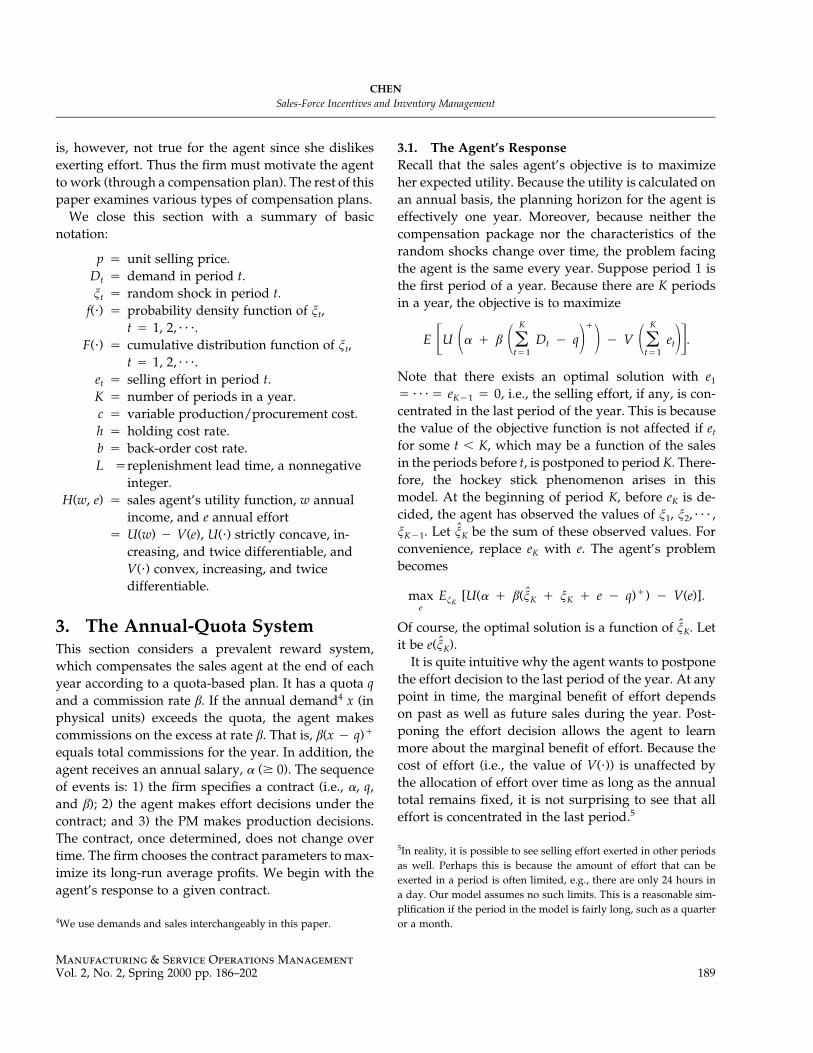
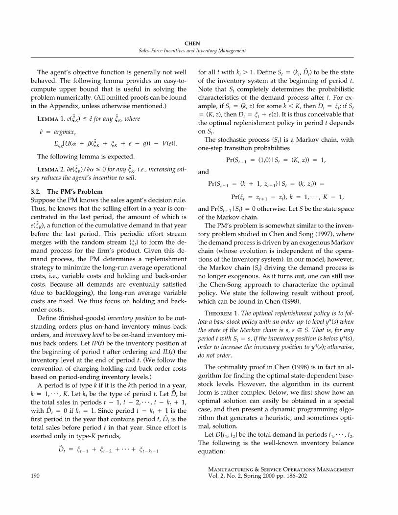
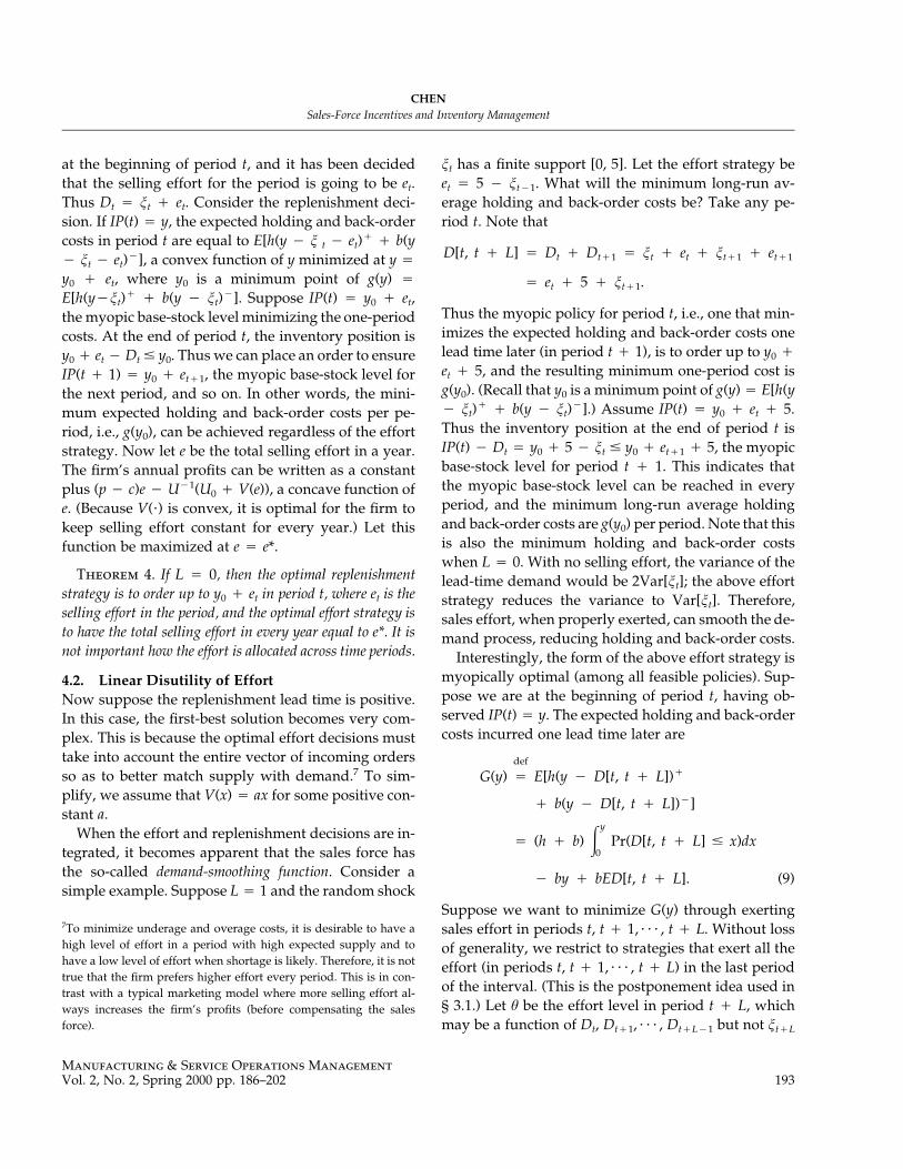
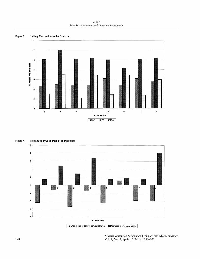
scenarios. Of course, the FB profits are always the high-est. MW is better than AQ only when the lead time islong (the even-numbered examples). This is intuitivebecause when the lead time increases, the benefit ofdemand smoothing becomes greater. This benefit isshown in Figure 2: MW is able to lower the holdingand back-order costs from the status quo, but not asmuch as FB can. Thus the unobservability of sellingeffort hinders the firm’s ability to induce the salesagent to smooth demand. Figure 3 shows the amountof selling effort exerted by the sales agent under thethree scenarios. The agent works harder under FB thanshe does under the other two scenarios. It is interestingto note that whenever MW outperforms AQ (in theeven-numbered examples), the sales agent expendsmore effort in MW than in AQ. So, does MW improveon AQ by extracting more surplus from the agent orby demand smoothing? Figure 4 answers this question,where net benefit from sales force (NBFS) is the firm’sgross revenue from selling effort, i.e., (p � c) * e, wheree is the expected annual effort minus the expected an-nual compensation received by the sales agent. Figure4 shows the change in NBFS and the decrease in in-ventory costs, as the firm switches from AQ to MW.Interestingly, MW often leads to lower NBFS and al-ways leads to lower inventory costs. Whenever the lat-ter outweighs the former, MW is better than AQ. Thissuggests that MW improves upon AQ via demandsmoothing, not by extracting more surplus from thesales force. Finally, Figure 5 shows that to reach FB,the firm must improve in both dimensions: NBFS as

well as demand smoothing. Exactly how this can bedone remains an open question.

7. ConclusionThe thesis of this article is that in designing a compen-sation package for its sales force, the firm ought to con-sider the impact of the sales-force behavior on itsproduct-delivery system. Generally speaking, a salespattern that exhibits large swings causes difficulties inproduction and distribution planning. It is thereforebeneficial to induce the sales force to exert selling effortin a way that smoothes the demand process. Toachieve this, the compensation package should havethe following features. 1) Incentive earnings (commis-sions and/or bonuses) should be based on the salesperformance in a time window whose length is deter-mined by the replenishment lead time. For example, ifit takes two months to replenish the finished-goods in-ventory, then incentive earnings should be based onquarterly sales. 2) After taking into account the admin-istrative costs and the psychological impact on thesales force, performance evaluation should be con-ducted as frequently as possible on a moving-time-window basis. For example, the sales force is evaluatedevery month based on its performance in the most re-cent quarter.9 This strategy can be beneficial to firmswith long lead times and significant costs associatedwith supply-demand mismatch.The sales-force incentive problem naturally lies in

the marketing-operations interface, and it should bestudied as such. It is our hope that future research willcontinue to investigate the different facets of thisproblem.

Appendix: Omitted ProofsProof of Lemma 1. Take any values of and nK. For any d � 0,nK

since � nK � e � d � q)� � � nK � e � q)� � d and U(•)ˆ ˆ(n (nK K

is increasing, we have

9An executive from Hewlett-Packard Company once suggested thatsalespeople should receive incentive earnings on their birthdaysbased on the performance in the most recent year. This is an inter-esting way to achieve demand smoothing with a multiperson salesforce. The author thanks Warren Hausman for this information.



Figure 1 Firm Profits and Incentive Scenarios

Figure 2 Inventory Costs and Incentive Scenarios



Figure 3 Selling Effort and Incentive Scenarios

Figure 4 From AQ to MW: Sources of Improvement



Figure 5 From AQ to FB: Sources of Improvement

�ˆU(� � b(n � n � e � d � q) )K K

�ˆ� U(� � b(n � n � e � q) � bd).K K

Therefore,

�ˆU(� � b(n � n � e � d � q) )K K

�ˆ� U(� � b(n � n � e � q) )K K

�ˆ� U(� � b(n � n � e � q) � bd)K K

�ˆ� U(� � b(n � n � e � q) )K K

ˆ� U(� � b(n � n � e � d � q))K K

ˆ� U(� � b(n � n � e � q)),K K

where the second inequality follows since U(•) is concave and �ˆ(nKnK � e � q) � � nK � e � q)�. Therefore, �EnKU (� � �ˆ ˆ(n b(nK K

nK � e � q)�)/�e � �EnKU (� � � nK � e � q))/�e. The lemmaˆb(nKfollows. ▫

Proof of Lemma 2. Define a � q � Thus the agent’s objectiven .Kfunction can be written as

�� a�e

U(� � b(x � e � a))f(x)dx � U(�)f(x)dx � V(e).� �a�e ��

Taking derivative of the objective function with respect to e and set-ting it to zero, we have the first-order condition:

��

b U�(� � b(x � e � a))f(x)dx � V�(e) � 0. (14)�a�e

Suppose e is a local maximum. Then, the second-order derivative isless than or equal to zero, i.e.,

��2b U�(� � b(x � e � a))f(x)dx�

a�e

� bU�(�)f(a � e) � V�(e) � 0. (15)

Differentiating the left-hand side of Equation (14) with respect to �

and rearranging terms, we have

��e 2[b U�(� � b(x � e � a))f(x)dx�a�e��

� bU�(�)f(a � e) � V�(e)]

��

� �b U�(� � b(x � e � a))f(x)dx�a�e

� 0,

where the inequality follows since U(•) is strictly concave. Thelemma follows by applying Equation (15). ▫

Proof of Theorem 2. Suppose L � 0. Let y0 be a minimum pointof E[h(y � nt)� � b(y � nt)�], a convex function of y. From Equation(1), yo(s) � y0 for all s � (k, z) � S with k � K, and yo(s) � y0 � e(z)for all s � (K, z) � S. It suffices to show that under the myopic base-stock policy, IP(t) � yo(s) for any t with St � s. Take any period t



with St � (K, z) for some z � 0. Suppose IP(t)� y0 � e(z), themyopicbase-stock level for period t. Since Dt � nt � e(z), the inventoryposition at the beginning of period t � 1 before ordering is y0 � e(z)� Dt � y0. Thus IP(t � 1) � y0 under the myopic base-stock policy.It is then clear that IP(t � 2) � • • • � IP(t � K � 1) � y0, whichimplies that IP(t � K) � y0 � e(z�) if St�K � (K, z�). ▫

Proof of Lemma 3. The lemma holds for k � K; see Equation (2).Now suppose it holds for k � 1. Take any z with (k, z) � S. Since (k� 1, z � nk) � S for any value of nk, the inductive assumption impliesthat EHk�1 (y � nk, z � nk) is convex in y. Recall that G(y|(k, z)) isconvex in y. From Equation (3), the lemma holds for k. ▫

Proof of Theorem 3. Suppose K � 2. Thus S � {(1, 0), (2, z), z� 0}. Clearly, Equation (5) holds for state (1, 0). Now take any state(2, z) � S. Note that yd(2, z) � yo(2, z) and (D[2, K]|(2, z)) � e(z).Thus Equation (5) holds for state (2, z) if yo(2, z) � e(z) � yd(1, 0).Given St � (2, z), D[t, t � L] is equal to e(z) plus a random com-ponent, denoted by D2. That is, D[t, t � L] � e(z) � D2. Define g(y)� E[h(y � D2)� � b(y � D2)�], a convex function minimized at,say, y2. Note that G(y|(2, z)) � g(y � e(z)) and thus yo(2, z) � y2 �

e(z). Now it only remains to show y2 � yd(1, 0). Recall that

dy (1, 0) � argmin [G(y|(1, 0)) � EH (y � n , n )] (16)y 2 1 1

and that

oH (w, z) � G(max{w, y (2, z)}|(2, z))2

o� g(max{w, y (2, z)} � e(z))

2� g(max{w � e(z), y }).

Thus H2(y � n1, n1) � g(max {y � n1 � e(n1), y2}), which, as a func-tion of y, is flat for y � n1 � e(n1) � y2 and is thus flat for y � y2.Consequently, EH2(y � n1, n1) is flat for y � y2. From Equation (16),to have y2 � yd(1, 0), it suffices to have

2 oy � y (1, 0), (17)

which we now verify. Let D1 be D[t, t � L] given St � (1, 0). ThusG(y|(1, 0)) � E[h(y � D1)� � b(y � D1)�]. If D1 is stochasticallylarger than D2, then Equation (17) holds. The exact relationship be-tweenD1 andD2 depends onwhether L is an even or an odd number.If, say, L � 1, then

1 2D � n � n � e(n ) and D � n � n .1 2 1 2 3

The former is stochastically larger. On the other hand, if, say, L �

2, then

1 2D � n � n � e(n ) � n and D � n � n � n � e(n ),1 2 1 3 2 3 4 3

which are stochastically the same. ▫

Proof of Theorem 5. Let w(•) andW(•) be, respectively, the p.d.f.and c.d.f. of X. Let be the c.d.f. of X � h(X).W(•)

Theorem 5(i): Because X � (B � X)� � B, Pr(X � (B � X)� �

x) � 0 for any x � B. Thus Theorem 5 (i) is true for z � B. Nowsuppose z � B. Because for any x � B, Pr(X � (B � X)� � x) �

W(x), it suffices to show

z z˜W(x)dx � W(x)dx. (18)� �

B 0

Because X � h(X) is stochastically larger than X, � W(x) for allW(x)x. Thus

� �˜[1 � W(x)]dx � [1 � W(x)]dx. (19)� �

z z

Because Eh(X) � E(B � X)� � W(x) dx, E[X � h(X)] � E[X �B�x�0

(B � X)�] can be written as� � B

˜[1 � W(x)]dx � [1 � W(x)]dx � W(x)dx.� � �0 0 0

The right side of the above equation can also be written as

� z B

[1 � W(x)]dx � [1 � W(x)]dx � W(x)dx� � �z 0 0

� z

� [1 � W(x)]dx � z � W(x)dx.� �z B

Therefore,� � z

˜[1 � W(x)]dx � [1 � W(x)]dx � z � W(x)dx, (20)� � �0 z B

which impliesz � �

˜ ˜ ˜[1 � W(x)]dx � [1 � W(x)]dx � [1 � W(x)]dx� � �0 0 z

(20) � z �˜� [1 � W(x)]dx � z � W(x)dx � [1 � W(x)]dx� � �

z B z

(19) z

� z � W(x),�B

which implies Equation (18).Theorem 5(ii): Because E[X � h(X)] � E[X � (B � X)�], it suf-

fices to show E[X � h(X)]2 � E[X � (B � X)�]2. Note that

� �2 2 2E[X � h(X)] � (x � h(x)) w(x)dx � x w(x)dx� �

0 0

� �2� 2xh(x)w(x)dx � h (x)w(x)dx� �

0 0

and that

B �� 2 2 2E[X � (B � X) ] � B w(x)dx � x w(x)dx� �

0 B

�2 2� B W(B) � x w(x)dx.�

B

Therefore, it suffices to show

B � �2 2 2x w(x)dx � 2xh(x)w(x)dx � h (x)w(x)dx � B W(B). (21)� � �

0 0 0

Because E[X � (B � X)�] � BW(B) � xw(x)dx and E[X � h(X)]��B� (x � h(x))w(x)dx, we have from E[X � h(X)] � E[X � (B ��0X)�]



B �

BW(B) � xw(x)dx � h(x)w(x)dx. (22)� �0 0

Note that

� B

h(x)w(x)dx � 2 (x � h(x))w(x)dx� �B 0

B � �

� 2 xw(x)dx � 2 h(x)w(x)dx � h(x)w(x)dx� � �0 0 B

(22) �

� 2BW(B) � h(x)w(x)dx � 2BW(B) � 2xW(B)�B

for all x � B. Therefore,

�

2x � h(x)�B �

� B

h(x)w(x)dx � 2 (x � h(x))w(x)dx� �B 0

� h(x)w(x)dx � 0W(B)

because the integrand is nonnegative. After some algebra, the aboveinequality implies

B � �2 2(x � h(x)) w(x)dx � 2xh(x)w(x)dx � h (x)w(x)dx� � �

0 B B2B �1

� x � h(x) � h(x)w(x)dx w(x)dx. (23)� � � �0 BW(B)

Note that the right side of Equation (23) is2B �1 w(x)

� W(B) (x � h(x) � h(x)w(x)dx) dx�� 0 BW(B) W(B)

B B1 1� W(B) xw(x)dx � h(x)w(x)dx� � �

0 0W(B) W(B)

2�1� h(x)w(x)dx� �

BW(B)

2B �1� xw(x)dx � h(x)w(x)dx��

0 0W(B)

(22) 1 2 2� (BW(B)) � B W(B),W(B)

where the first inequality follows since w2 is convex in w. The firstpart of Theorem 5(ii) follows by noting that the left side of Equation(23) is equal to the left side of Equation (21).

The second part of Theorem 5(ii) follows since

� � 2 � 2Var[X � (B � X) ] � E[X � (B � X) ] � (E[X � (B � X) ])� �

2 2 2� B W(B) � x w(x)dx � (BW(B) � xw(x)dx)� �B B

and

�dVar� 2W(B) B � (BW(B) � xw(x)dx)� � �

BdB

�� 2W(B) [B � E[X � (B � X) ]]

� 0. ▫

ReferencesBaiman, S. 1982. Agency research in managerial accounting: A sur-

vey. J. Accounting Literature 1 155–213.Basu, A., R. Lal, V. Srinivasan, R. Staelin 1985. Salesforce-

compensation plans: An agency theoretic perspective. Market-ing Sci. 4 (4) 267–291.

Chen, F. 1998. Salesforce incentives and inventory management.Working paper, Graduate School of Business, Columbia Uni-versity, New York, NY.

———, J. Song. 1997. Optimal policies for multi-echelon inventoryproblems with Markov modulated demand. To appear inOper.Res.

Churchill, G., Jr., N. Ford, O. Walker, Jr. 1993. Sales Force Manage-ment. Irwin, Homewook, IL.

Coughlan, A. 1993. Salesforce compensation: A review of MS/ORadvances. J. Eliashberg, G. Lilien, eds. Handbooks in OperationsResearch and Management Science: Marketing, vol. 5. North-Holland, Amsterdam, The Netherlands.

———, S. Sen. 1989. Salesforce compensation: Theory and manage-rial implications. Marketing Sci. 8 (4) 324–342.

Davis, O., J. Farley. 1971. Allocating sales force effort with commis-sions and quotas. Management Sci. 18 (4) (Part II) P-55–P-63.

Dearden, J., G. Lilien. 1990. On optimal salesforce compensation inthe presence of production learning effects. Internat. J. Res. Mar-keting 7 (2–3) 179–188.

Farley, J. 1964. An optimal plan for salesmen’s compensation. J. Mar-keting Res. 1 (2) 39–43.

———, C. Weinberg. 1975. Inferential optimization: An algorithmfor determining optimal sales commissions in multiproductsales forces. Oper. Res. Quart. 26 (2) 413–418.

Grossman, S., O. Hart. 1983. An analysis of the principal-agent prob-lem. Econometrica 51 (1) 7–45.

Harris, M., A. Raviv. 1978. Some results on incentive contracts withapplications to education and employment, health insurance,and law enforcement. Amer. Econom. Rev. 68 (March) 20–30.

———, ———. 1979. Optimal incentive contracts with imperfect in-formation. J. Econom. Theory 20 (April) 231–259.

Holmstrom, B. 1979. Moral hazard and observability. Bell J. Econom.10 (1) 74–91.

———. 1982. Moral hazard in teams. Bell J. Econom. 13 (2) 324–340.———, P. Milgrom. 1987. Aggregation and linearity in the provision

of intertemporal incentives. Econometrica 55 (March) 303–328.Lal, R. 1986. Delegating pricing responsibility to the salesforce.Mar-

keting Sci. 5 (2) 159–168.———, V. Srinivasan. 1993. Compensation plans for single- and

multi-product salesforces: An application of the Holmstrom-Milgrom model. Management Sci. 39 (7) 777–793.

———, R. Staelin. 1986. Salesforce-compensation plans in environ-ments with asymmetric information. Marketing Sci. 5 (3) 179–198.

Porteus, E., S. Whang. 1991. On manufacturing/marketing incen-tives. Management Sci. 37 (9) 1166–1181.

Raju, J., V. Srinivasan. 1996. Quota-based compensation plans for



multiterritory heterogeneous salesforces. Management Sci. 42(10) 1454–1462.

Rao, R. 1990. Compensating heterogeneous salesforces: Some ex-plicit solutions. Marketing Sci. 9 (4) 319–341.

Shavell, S. 1979. Risk sharing and incentives in the principal andagent relationship. Bell J. Econom. 10 (1) 55–73.

Srinivasan, V. 1981. An investigation of the equal commission ratepolicy for a multi-product salesforce. Management Sci. 27 (7)731–756.

Tapiero, C., J. Farley. 1975. Optimal control of salesforce effort intime. Management Sci. 21 (9) 976–985.

Weinberg, C. 1975. An optimal commission plan for salesmen’s con-trol over price. Management Sci. 21 (8) 937–943.

———. 1978. Jointly optimal sales commissions for nonincomemax-imizing salesforces. Management Sci. 24 (12) 1252–1258.

Zipkin, P. 1989. Critical number policies for inventory models withperiodic data. Management Sci. 35 (1) 71–80.

The consulting Senior Editors for this manuscript were Morris Cohen and Jehoshua Eliashberg. This manuscript was received on February 1, 1999, andwas with the author 105 days for 1 revision. The average review cycle time was 109.5 days.

sales-forceincentivesandinventory management · sales-forceincentivesandinventory ......

Documents