sales - ted whitmer companies sales comparison approach is every appraiser’s favorite approach...

Sales

Table of ContentsChapter 1 Sales Comparison Approach Concepts 1Chapter 2 Units of Comparison 11Chapter 3 Elements of Comparison 13Chapter 3 Elements of Comparison 13Chapter 4 Sales Analysis 21Chapter 5 Condemnation 37

Ted Whitmer, MAI

College Station, TX 77845Phone: (979) 690 9465Phone: (979) 690-9465

Email: [email protected]: www.tedwhitmer.com

2508 Merrimac Ct

NOTES This page left intentionally blank.

Chapter 1 Sales Comparison Approach Concepts

The sales comparison approach is every appraiser’s favorite approach when there is adequate data and information to adjust the sales. All appraisers are good when they are appraising a property and have sales on both sides of the subject, three across the street. This is especially true when they are exactly like the subject and sold for the exact same price. However, this is seldom the case in appraising, especially when the property is subject to litigation. Furthermore, the property interest that sells and the property interest appraised are often different. Property tax and condemnation appraisals are generally of the fee simple interest, while the sales of leased properties are leased fees. If there is a sale of a property without a lease, often it is still not exactly comparable because there is generally an assumption of market occupancy for a fee simple valuation. Besides the property interest, the definition of value used in the case must be applied to the subject valuation and compared to the actual conditions behind the sale. The following premises are usually required by “market value.” ♦ Most probable or highest price ♦ In terms of cash ♦ No concessions ♦ Willing buyer & seller ♦ Acting in their own best interests ♦ Typically motivated ♦ Well informed ♦ Property exposed for a reasonable length of time ♦ Competent management ♦ Highest & best use ♦ It is a gross value, including commissions and closing costs ♦ It is usually defined as a point in time estimate (opinion)

The appraiser must select units of comparison that help explain differences in prices. Furthermore, the elements of comparison must be applied to the units of comparison to adjust the comparable to the subject.

Relationship to appraisal principles Supply & demand – Prices paid are a function of the supply relative to the demand for the product. Substitution – A buyer will not pay more than for an equally useful substitute property. Balance – It is when the agents of production are in their proper mix. Externalities – Real estate is fixed in location and dependent upon surrounding properties and linkages.

Linkages are time and/or distance relationships between a property and work, play, shopping, etc.

Procedure Research - Sales, listings, contracts, etc. Verify – To verify is to establish that the information is a fact. To confirm is remove doubt about the fact. Unit of comparison(s) – Ways to look at value such as psf, per unit, overall price, etc. Compare sales with elements of comparison – The adjustment factors. Reconcile – Using judgment to take all information and come to a conclusion about value, etc.

Sales

Copyright Ted Whitmer. All rights reserved.

1 Sales

Sales Comparison ApproachApproach

Quantitative Qualitative MethodsMethods

Paired data (One pair)Grouped data

MethodsRelative comparison

Up, down & thereforeGrouped data

by independent variable

Statistical Graphical

Ranking Ascending or descending orderPersonal interviewsp

Sensitivityisolate affect of variable

Trend

AdjustmentsDollar or percentage

CostSecondaryDirect comparisons (Grid)

OrderElements of Comparison

Capitalization of rent differences

Units of Comparison

Sales


2 Sales

Let’s Be Reasonable

Does the market have to do the approach like we do it to be a valid approach?

Wh t if th h l i What if the approach explains the actions of buyers & sellers?

Does the market do 3 approaches?

Does the residential market even do an adjustment grid?

Sales


3 Sales

Reasonableness as to Rate SelectionSe ec o

Can we apply a rate derived pp yfrom annual year-end-accounting models to another frequency?frequency?

Can we adjust for horizontal or Can we adjust for horizontal or vertical risk?

Can we adjust for fee simple, leased fee or leasehold valuations?valuations?

Can we adjust multipliers?Can we adjust multipliers?

Sales


4 Sales

Reasonableness of the Single P i E ior Point Estimate

If the data applied indicate a range of value, then the most “conservative” answer is in the middle.

The point estimate is as reliable as…the appraiserthe datah l i f h d i li h f ll the analysis of the data in light of all other market evidence

Sales


5 Sales

Reasonableness of Three Approachespp oac es

Cost approachppdoes not set upper limit of valuedoes not end in cost

Income approachdoes not set lower limit of valueis not an investment value in appraisals requiring market value

Sales comparison approachis not always the best approachdoes not require pairing sales

Sales


6 Sales

Reasonableness of Rounding

Do you round to more than Do you round to more than your annual income in one appraisal?Rounding rules in science:◦ Round after every calculation◦ Use the least precise “significant ◦ Use the least precise significant

digits”

Rounding rules in appraising:◦ Ignore rounding rules in science◦ Use reasonable rounding

Sales


7 Sales

Tests of R blReasonableness

Rules of thumbRules of thumbIncome multipliers

1/3, 1/3 & 1/3 rule

etc.

Between approachesAge expressed in depreciation?

Obsolescence expressed in sales comparison & income p papproaches?

Risk in income approach show up in sales & cost approaches?

Adjustments make sense in all three approaches?Adjustments make sense in all three approaches?

Does property interest reflect cost approach (fee simple without adjustments) & sales comparison approach (often leased fee sales)?

Are approaches over-adjusted?

Is income that rate is applied to similar from income the rate is derived from?

Sales


8 Sales

Reasonableness as to Overall ValueOve a Va ue

If ld b h If you would buy the property for the appraised value, you probably underappraised it!What does the history of the property tell us?What were past listing prices?What were past listing prices?Are you too optimistic in a growth market or too pessimistic i d k ?in a down market?Were you steered by your client?

Sales


9 Sales


Sales


10 Sales

Chapter 2 Units of Comparison

Definition – Components a property can economically or physically be divided into for comparison and analysis purposes. Is usually expressed as e.g. $100 psf. Rentals are expressed as e.g. $10 psf per year (a time period is given as a qualifier).

Examples of units of comparison 1. Farms Bushels, pounds of production, bales, etc. 2. Ranches Animal units (be careful of price per acre) 3. Ski resorts Skiers per day, lift tickets sold, Lifts per day 4. Golf courses Rounds per day, acres, linear 5. Day care facilities Licensed child capacity 6. Warehouses Cubic or square foot 7. Retail/fast food restaurant Look per site, per square foot 8. Churches Per seat, per pew 9. Residential lots Per lot, per front foot, per square foot 10. Apartments Per square foot, per unit, per room, per bedroom

Selection of a unit of comparison - Consider the following How would an investor look at the property to purchase based upon productivity of the

capital invested?

How are the rental rates quoted? This may give an indication of a reasonable unit of comparisons.

If two potential units of comparison are per size (e.g. psf, per acre) and per economic

characteristic (e.g. per licensed child capacity, per animal unit), then the best unit of comparison is probably going to be the economic characteristic. However, you may want to initially analyze based upon both. The appraisal of a ranch may indicate sale prices at $500 to $2,000 per acre, but $500 to $750 per animal unit. The price per animal unit would be the most appropriate to use.

Use multiple units of comparison and reconcile the indications. For example, look at a golf

course per acre, per hole, per rounds played, per lineal foot of yardage, etc. and reconcile the conclusions giving the most weight to the unit that is the best indicator of value.

Sales


11 Sales

Property Types & Subtypes Units of Comparison?

Agricultural

1. Agribusiness a. Aquaculture b. Dairy c. Grain elevator d. Greenhouse/nursery e. Livestock farms

2. Pasture/ranch 3. Permanent crops 4. Row crops 5. Timberland 6. Undeveloped agricultural

Assembly/Meeting Place

1. Armory/club/lodge facility 2. Community/recreation center 3. Convention center 4. Reception hall/banquet facility 5. Religious facility

Health Care

1. Acute care hospital 2. Ambulatory surgery center 3. Behavioral care facility 4. Clinical laboratory 5. Comprehensive ambulatory care

center 6. Medical center 7. Medical office 8. Rehabilitation center/hospital

Industrial

1. Flex space 2. Industrial-business park 3. Industrial condominium 4. Intermodal facility 5. Manufacturing (Heavy, light,

high-tech) 6. Office/showroom 7. Processing/production/refinery

facility (Chemical, energy, food, mineral, water)

8. Research & development (R&D) 9. Salvage yard 10. Sawmill/lumberyard 11. Self-storage/mini-storage facility 12. Tank farm/petroleum storage 13. Truck terminal/hub/transit

facility 14. Underground/cave storage 15. Warehouse (air cargo,

distribution warehouse, loft/multi-storage, refrigerated/cold storage, storage warehouse)

Land

1. Undeveloped agricultural

2. Easement (Conservation/preservation, flowage, right-of-way)

3. Industrial 4. Multifamily (apartment, duplex,

etc.) 5. Office 6. Park/open space 7. Residential (single-family) 8. Retail 9. Retail pad 10. Water-related (coastal/island,

flood zone, wetland/marshland) 11. Wilderness

Lodging and Hospitality

1. All-suite 2. Bed & breakfast 3. Campground/RV-trailer camp 4. Casino hotel 5. Convention hotel 6. Economy/limited service 7. Extended-stay 8. Full-service 9. Luxury 10. Mixed-use (Hotel-office, hotel-

office-retail, hotel-retail) 11. Resort/spa

Multifamily

1. Garden/low rise 2. Government-subsidized 3. Mid/high-rise 4. Mobile/manufactured housing 5. Student-oriented housing

(dormitory, fraternity/sorority, student-oriented apartment)

Office

1. Creative/loft 2. Office building (low, mid, high-

rise) 3. Institutional/governmental 4. Medical 5. Mixed-use (office and industrial,

multifamily, retail, retail & industrial, retail & multifamily)

6. Office/business park 7. Office/R&D 8. Office/warehouse

Retail-Commercial

1. Car wash (full-service, hybrid, self-service)

2. Convenience store 3. Day care/nursery 4. Garden center

5. Mixed-use (with office, or residential)

6. Parking (garage & surface) 7. Post office 8. Restaurant (fast food, full-

service, limited service, sit down)

9. Mulit-screen/megaplex theatre 10. Retail-pad 11. Tavern, bar, nightclub,

microbrewery 12. Service station/gas station 13. Single-screen theatre 14. Freestanding building (bank

branch, big box, department store, grocery, freestanding)

15. Street retail 16. Vehicle-related (dealership, lube,

tire, service & repair) Senior Housing

1. Assisted living 2. Congregate senior housing 3. Continuing care retirement 4. Skilled nursing

Shopping Center

1. Community 2. Convenience/strip 3. Fashion/specialty 4. Neighborhood 5. Outlet 6. Power center 7. Regional 8. Superregional mall 9. Theme/festival

Special Purpose

1. Airport/hanger 2. Cemetery/mausoleum 3. Courthouse 4. Funeral home/mortuary 5. Jail/correctional facility 6. Landfill 7. Library 8. Marina 9. Military facility 10. Mine/quarry 11. Museum/gallery 12. Outdoor signs 13. Salvage yard 14. Sawmill/lumberyard 15. School/university 16. Tank farm/petroleum storage 17. Train station/bus terminal 18. Truck terminal/hubtransit facility 19. Zoo/nature facility

Sales


12 Sales

Chapter 3 Elements of Comparison

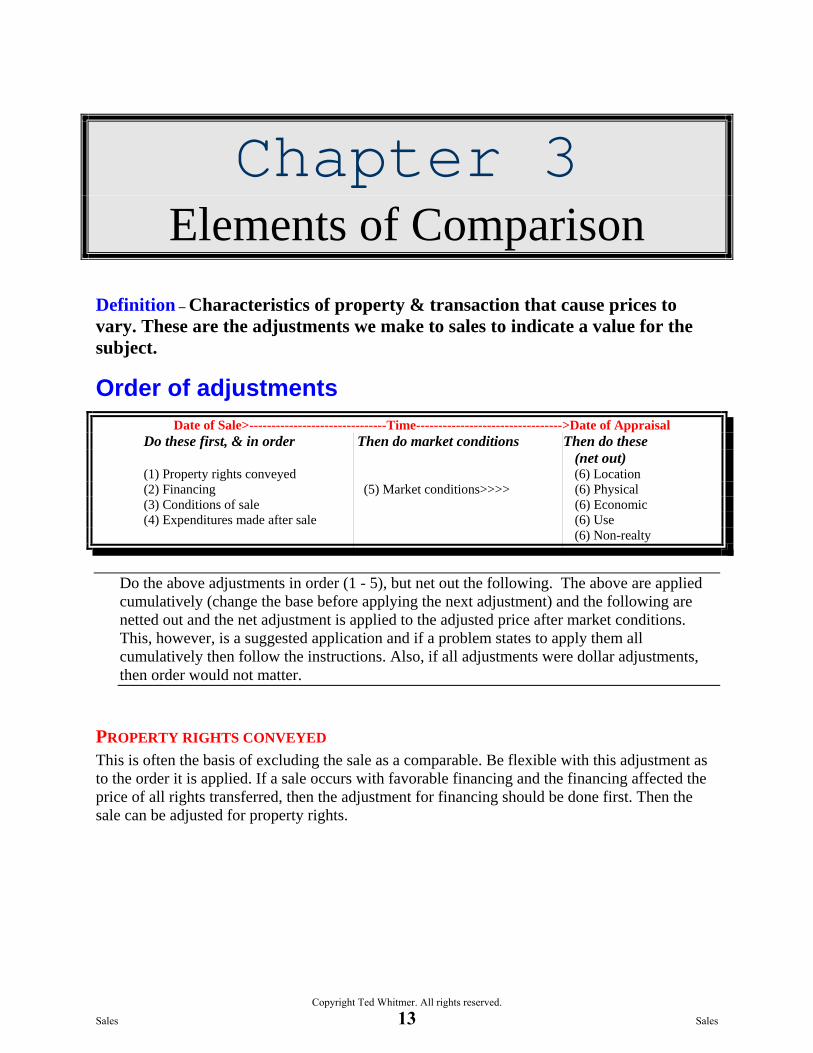
Definition – Characteristics of property & transaction that cause prices to vary. These are the adjustments we make to sales to indicate a value for the subject.

Order of adjustments Date of Sale>-------------------------------Time--------------------------------->Date of Appraisal Do these first, & in order Then do market conditions Then do these (net out) (1) Property rights conveyed (6) Location (2) Financing (5) Market conditions>>>> (6) Physical (3) Conditions of sale (6) Economic (4) Expenditures made after sale (6) Use (6) Non-realty

Do the above adjustments in order (1 - 5), but net out the following. The above are applied cumulatively (change the base before applying the next adjustment) and the following are netted out and the net adjustment is applied to the adjusted price after market conditions. This, however, is a suggested application and if a problem states to apply them all cumulatively then follow the instructions. Also, if all adjustments were dollar adjustments, then order would not matter.

PROPERTY RIGHTS CONVEYED This is often the basis of excluding the sale as a comparable. Be flexible with this adjustment as to the order it is applied. If a sale occurs with favorable financing and the financing affected the price of all rights transferred, then the adjustment for financing should be done first. Then the sale can be adjusted for property rights.

Sales


13 Sales

FINANCING OR CASH EQUIVALENCE

Decision Tree 1. Seller carries a note Discount the note to market 2. Seller sells with an assumable note Discount the note to market 3. Seller pays points on buyer’s note Deduct the amount of points (compute on the

loan amount & not sale price!) 4. Seller “wraps” a first note Discount the debt the owner carries to market 5. Paired sales show price is affected Adjust the sale price 6. Owner sells note after sale for less/more Deduct or add the discount or premium 7. Market indicates a flat discount Apply 1 - % of flat discount to loan amount 8. Seller Rm & market Rm given Loan x Rm to seller divided by Rm from

market

Discounting a Note - (3 Step Process) 1. Calculate the payments on the note at the contract, not the market rate and the contract, not the market

term. 2. If necessary, calculate the balance of the loan at the contract, not the market rate by either: a. By the contract terms; e.g. “the loan balloons in 5 years”, or b. The “average life” of the loan 3. Leave the above in the calculator, put the market rate of interest in i and solve for PV. NOTE: Cash equivalency adjustments are a 4 step process when the seller carries a note. Do the above 3 steps and

add the down payment back to the value of the note derived in the three steps above.

Example

Seller carries a note for $100,000 at 7%, 240 months with a 10 year call provision. The market rate for similar notes is 10%. What is the value of the note. N i PV PMT FV Step 1: Payment at contract 240 7/12 100,000 [775.30] Step 2: Balance at contract 120 [66,774] Step 3: Discount at market rate 10/12 [83,334] 1. What if the seller carries a note and pays points for the buyer to get a first note?

Answer: Discount the note carried by the seller to market and deduct points.

2. What if the seller pays points and the buyer gets a favorable note from his parents? Answer: Deduct the points paid by the seller and don’t do anything with the note.

3. What if the seller transfers a note with a favorable rate on the sale to a buyer?

Answer: Discount the note to market at a rate that reflects the risk position of the assumed note.

4. What if the seller carries a note at a below market rate, but tells you it did not affect the sale price? Answer: Compare the sale price to other sales to see if that looks reasonable.

Sales


14 Sales

Related Problem: A buyer purchases a property worth $2,000,000 for $2,300,000 with a note for $2,000,000, interest only at 10%, monthly payments and a balloon in 8 years. What was the discount rate applicable to the note?

Answer: The cash equivalent price is given at $2,000,000. The question is what is the rate that will discount the note to $1,700,000 (there is $300,000 down).

N I PV PMT FV

96* [Compute:1.0857 x 12 =13.03%] -1,700,000 16,667** 2,000,000***

**8 x 12 = 96 months

**The payment is $2,000,000 X .10 divided by 12 = 16,667 ***The note is interest only, so does not reduce.

CONDITIONS OF SALE (MOTIVATION) Example: Ten lots were purchased at a 45% discount to one buyer for $100,000, or $10,000 each. If comparing the individual lots to a subject lot, what percentage would you have to adjust the sales price to get the indication of value for the subject? Assume the subject is worth the price of the lot in the comparable before discounting. [Note: This is an example of how percentages can be confusing more than it is an example of how to do a conditions of sale adjustment.] Lot price without discounting X (1 – 45%) = $10,000 Lot price without discounting X .55 = $10,000 Lot price without discounting = $10,000/.55 = $18,182 To adjust the $10,000 lot to $18,182, an upward adjustment of 81.81% would be necessary. [10,000 ENTER 18,182 ∆%, Display: 81.82%]

EXPENDITURES MADE AFTER SALE This category should be broadened to any known adjustment that is relevant as of the date of sale (other than property rights, financing and conditions of sale). The adjustment should be made prior to a market conditions adjustment because it is relevant as of the date of sale and not after a time adjustment.

Example: A buyer bought property for $125,000 and spent $25,000 in repairs immediately after purchase. The market conditions have resulted in an increase in prices of 10% since the date of sale. Appraise the subject as in good repair, what is the indicated value? Adjust first for the expenditure: $125,000 + 25,000 = $150,000 Then adjust for market conditions: $150,000 x 1.10 = $165,000

Sales


15 Sales

MARKET CONDITIONS (TIME) A sale happened 18 months ago for $100,000 and recently sold for $125,000, what is the straight-line and compound time adjustments? Sale 2 occurred 14 months ago for $95,000, what is the adjusted price? Straight-line: 100,000 ENTER 125,000 ∆% [Display: 25%] divide by 18 [Answer: 1.38%/mo., or .0138 as a decimal]

Compound: N I PV PMT FV 18 [Calculate:1.25%] -100,000 125,000 Note: The compound adjustment for the same sale is less per month than straight-line because the base of the percent changes every month to the new price. The straight-line adjustment is made on the original price every month; therefore, the base of the adjustment is smaller and a larger percent is required to achieve the same adjusted price (in this example the $100,000 is adjusted to $125,000 over 18 months either straight-line at 1.38% or compounded at 1.25%).

To adjust the sale of $95,000 over 14 months, use the percentage adjustment extracted from the sale.

Straight-line: 95,000 x (1 + .0138 x 14) = $113,354

Compound: N I PV PMT FV 14 1.25 -95,000 [Calculate: $113,046] Note: The application of the straight-line and compound adjustment gives a slightly different answer because the adjustment was over 14 and not 18 months as it was extracted.

Important: Read the question and if the market conditions adjustment is given, then calculate it as given, if there are two sale and resales, you may compute both ways and see which gives a tighter indication. If for example, if two sale & resales shows a compound time adjustment of 1% and 1.3%, but the indicated straight-line adjustments are 1.15% and 1.2%, then use a 1.2% straight-line adjustment to the sales.

YOU MUST APPLY THE ADJUSTMENT IN THE WAY YOU DERIVE THE ADJUSTMENT!!!

Sales


16 Sales

THE FOLLOWING HAVE NO ORDER & THEY ARE NETTED OUT ♦ LOCATION ♦ PHYSICAL ♦ ECONOMIC CHARACTERISTICS ♦ USE ♦ NON-REALTY COMPONENTS OF VALUE

For example: An adjusted price, after financing, conditions of sale, expenditures made after sale, and market conditions is $100,000. Assume a location adjustment of 10%, a size adjustment of –10%, an occupancy adjustment of 10%, a use adjustment of –5% and an adjustment for personal property of –5%, the adjusted sale is still $100,000 because all the adjustments netted out to 0%.

Rules for order of adjustments

If you have all dollar adjustments, it doesn't matter

If you have some percentage adjustments, do (1) - (5) in order, then net out the rest (6) - (10).

If you have all percentage adjustments, it doesn't matter if you mathematically apply them all the same way.

Sales


17 Sales

Adjustments on the Time Line - Example: Single-family house

Assume a sale of a house for $250,000. Also assume the following adjustments. (1) Location $10,000 (2) Financing 10% (3) Physical - 2,000 (4) Market conditions - 8% (5) Expenditure after sale 5,000 (6) Non-realty components 10% (7) Real property rights conveyed - 5% (8) Conditions of sale 3,000 The adjustments of (1) real property rights conveyed, (2) financing, (3) conditions of sale, and (4) expenditures made after sale are made as of the date of sale. The resulting adjusted price from above is then adjusted to the date of valuation. The remaining adjustments are from that adjusted price and are netted out. There is no order of adjustments after market conditions. Comparable sale price $250,000 (1) Real property rights - 12,500 [250,000 x -5%] $237,500 (2) Financing 23,750 [237,500 x 10%] $261,250 (3) Conditions of sale 3,000 $264,250 (4) Expenditure after sale 5,000 $269,250 (5) Market conditions - 21,540 [269,250 x -8%] $247,710 Note: This is the adjusted price to the date of valuation after adjusting in order the first four adjustments as of the date of sale. The remaining adjustments are derived from this number as the base of any percentage adjustment and are netted out. (6) Physical & location 8,000 [Location $10,000 & physical -2,000] (7) Non-realty components 24,771 [247,710 x 10%] Adjusted price $280,481

Problem (Going backwards): The adjusted sale price is $10 psf and it sold 10 months ago. Appreciation is 5% per year (straight-line). There was a +20% density adjustment, a +10% location adjustment and a –5% age adjustment. What was the price before adjusting?

Answer: Price X (1 + .05(10/12) X (1 + .20 + .10 - .05) = $10 Price X (1.041667) X 1.25 = $10 Price X 1.3020833 = $10 Price = 10/1.3020833 = $7.68

Sales


18 Sales

Order of adjustmentsOrder of adjustmentsSuggested

Date of Sale>------------------Time-------------->Date of AppraisalDo these first, & in order. Then do market conditions. Then do these (net out).

In no particular order.

(1) Property rights conveyed| | (6) Location(2) Financing | (5) Market conditions>>> | (6) Physical(3) Conditions of sale | | (6) Economic(4) Expenditures made | | (6) Use

after sale

However,

(1) If there is special financing, wouldn’t this also affect the property rights conveyed sale price? (If the real property is worth $700,000, personal property worth $200,000 & intangibles worth $100,000 & price affected $250,000 by intangibles worth $100,000 & price affected $250,000 by favorable terms, the favorable terms would affect all parts of the transaction.)

(2) Shouldn’t all dollar adjustments that are provided as of the date of sale be adjusted before a market conditions adjustment? (If a buyer tells you that location was worth $5.00 psf versus where the subject is located, as of when he bought it, the adjustment should be before a market conditions adjustment.)conditions adjustment.)

Sales


19 Sales


Sales


20 Sales

Chapter 4 Sales Analysis

Comparables Selection Highest & best use - The most important consideration when analyzing sales is to use comparables with the same highest and best use. Not just general category, but subcategory of use.

DO NOT BE AFRAID TO EXCLUDE A BAD “COMPARABLE.” Often appraisers lean on relatively few (or one) sale(s) if the one or few seem to be in line with other market indications and sales. Exclude sales or rentals of dissimilar use or ones that get in the way of determining adjustments or value. What is the better comparable, the site adjacent to the corner gas station site used for fast food or another gas station site across town? Is a suburban office building the same highest and best use as a downtown? If the subject is a community shopping center, would the best comparable be a regional mall or neighborhood center, or would an older community shopping center sale be more useful? Bottom Line: Compare properties in the same subcategory, not just the five general categories listed below. What are the 5 general categories of use?

Residential Commercial Industrial Agricultural Special use

“Best comparable” – is the one that is the same highest and best use as the subject, and then the overall smallest number of total adjustments, not net adjustments. A comparable can be adjusted 100%, but with a net 0% adjustments.

Organization of data If a simple property, then a grid. If a complex property, then another way. First chose one or more units of comparison, then… • Arrange the sales data by date of sale • Arrange the sales data by age of property • Arrange by highest to lowest NOI psf (However, avoid using a regression). • Arrange by location, size, or look at the questions & see what might be an important consideration • Place the sales on a simple graph. The y-axis is sale price & the x-axis some independent variable. • By comparing two different units of comparison such as price psf and price per unit in multifamily and

correlating to a reasonable value. • Be creative, see how the income is generated on income producing properties & order according to an

economic unit of comparison.

Sales


21 Sales

Adjustments Paired Sales - direct comparisons

Inferred - direction of adjustment (objective), but not quantity of adjustment (this is the judgment).

For example: A corner commercial property (the subject) is identical to another commercial site that sold for $10 psf except the subject has 10% better traffic (both quality and quantity). What is the adjustment for the traffic?

We would all agree that the adjustment would be a “+” adjustment. However, if the +10% traffic resulted in +10% sales, then the adjustment may be greater than 10%. It is possible that 10% increased sales could result in additional profit of 20% for some commercial endeavors. A purchaser may pay more than 10% more for the subject.

Percentage vs. dollar adjustments Most quantified adjustments are dollar adjustments. A percentage adjustment is problematic because there is a question as to what the base of the adjustment should be. Follow the suggested order of adjustments unless led another way by a problem (or the market). When extracting adjustments, extract them as dollar adjustments (except a market conditions adjustment) and do not make them percentage adjustments unless the questions on the test are set up that way. The following are two examples of misused percentage adjustments.

Example 1: Utility adjustment that is $25,000/acre when comparing two comparables with and without utilities. The adjustment was $25,000 divided by $50,000 or 50%. Two tracts sold for $60,000 & $100,000 respectively. Both need adjustments for utilities. If the percentage is used, the adjustments are $30,000 and $50,000. However, utility adjustments are generally based upon the money necessary to get utilities to a site. The amount is not dependent upon the value of the raw land. Both tracts should be adjusted $25,000 per acre unless other information leads you to another adjustment.

Example 2: A 10% upward & 10% downward adjustment. A site sold for $100,000 with a corner and a site sold on the same block for $90,000 without a corner. All other attributes are equal. The adjustment is 10% with the $100,000 as the base, and 11.1% with the $90,000 as the base. Furthermore, many appraisers use the extracted adjustment across prices such as $50,000 or $200,000 sites. The adjustments would be $5,000 or $20,000 at 10%. Furthermore, the 10% adjustment would not be appropriate regardless of the direction of the adjustment (+10% and –10% to different comparables).

Sales


22 Sales

If a comparable sold for $100,000 and is 10% superior to the subject, what is the value of the subject? Answer: C = 1.10 X S $100,000 = 1.10 X S S = $100,000/1.10 = $90,909 If A is 15% inferior to B, C is 10% superior to B, and C is 20% inferior to D, what is the percentage adjustment from A to D? Procedure: 1. Convert the sentences to equations. The “is” in the sentence is the equal sign.

For example: A = 15% inferior to B “Inferior” means the number multiplied into the letter or word to the right of the equality will be less than one. “Superior” means add the percentage to one. Therefore, the number will be greater than one. For example: A = (1 – 15%) X B, or A = .85B [Convert all the sentences to equations in a similar way.] A = .85B C = 1.10B C = .80D

2. Make up a number, such as 100 for one of the letters. It is easiest to make up a number for the letter that appears most frequently on the right side of the equal sign. However, the answer is the same no matter which letter you make up the number for. I will use B = 100.

3. Substitute the made up number in place of the letter. A = .85 (100) = 85 C = 1.10 (100) = 110 C = .80 D

4. Substitute the calculated numbers and solve for all letters. 110 = .80 D 110/.80 = D D = 137.5

5. To adjust A to D, use the ∆% key. Put in the value of A & ENTER, then the value of D and hit ∆%. [85 ENTER 137.5 ∆%] [Display: 61.76%]

Identification and Measurement of Adjustments Quantitative 1. Paired data - used to isolate one adjustment. See direct comparisons for more than one adjustment to many

sales. Example: A property sold in 1/96 for $100,000. The owner added a bathroom for $7,500 and sold the house shortly

afterward for $115,000. The extra bath from sale and resale is worth $15,000 in this market. A property sold in 5/96 for $100,000 and sold in 5/97 for $110,000. The market indicates a 10% increase in prices

from this sale. 2. Grouped data analysis - grouping data by independent variable such as size, date of sale, etc. 3. Statistical analysis - Inference or regression Example: The following regression is sale price psf against size of homes. The vertical line from the x-axis to the

regression line represents the size of the subject. The horizontal line from the regression line to the y-axis shows the indication of value psf for the subject size.

4. Graphic analysis - Visual interpretation. Three graphs of sales follows the regression graph.

Sales


23 Sales

Regression Assume the dotted line represents the subject of an appraisal. What is the size and value of the subject? Is r (correlation coefficient) negative or positive? Is r2 positive or negative? What is the approximate slope of the line? What is the y-intercept? The size of the “subject” appears to cross at about 2,175 sf and the value at the y-axis is approximately $122 because each interval appears to represent $20 psf when going from $60 to $200 psf. The line is sloping downward. Therefore, the correlation coefficient (r) is negative. The coeffecient of determination r2 is always positive. The slope of the line is the change in y divided by the change in x (∆y/∆x). At 1,600 sf y = approximately $160 and at 2,700 sf y = approximately $100 psf. Therefore, the slope is (100 – 160)/(2,700 – 1,600) = -3/55. The line drawn out

would intercept the y-axis at approximately $178. The equation of the line is y = -3/55x + 178

Price psf

Size 1,500 sf 2,500 sf2,000 sf

$ 200

$60

Sales


24 Sales

Sales Graph 1 What is being represented in this graph? What can be said about the desirability of the various tracts represented by A , B & C?

Sale price psf

Size

A

B

C

The graph represents size as the independent variable and sale price psf as the dependent variable. The curve begins upward sloping which means the price psf gets higher as the size increases. The price psf is highest at point B. The curve becomes downward sloping and the price psf gets smaller to point C. This is probably representing a highest and best use where the properties to the left of B are too small for the optimal use and are too large to the right of B. Desirability is based upon the overall value of a property and not the price psf. If the x & y axis were labeled then the overall desirability could be determined. However, with what is given it cannot be determined. B is not necessarily more desirable than C, just because the value psf is higher. If C were large enough, it would be worth more even with a smaller unit value psf.

Sales


25 Sales

Sales Graph 2

What is being represented in this graph?

Price PSF

Size

This appears to be the flip on the preceding graph. The sale price psf is getting smaller to a point, then it gets larger again as the size increases. This could possibly be representing the utility of properties across two different highest and best uses. The properties become too large for the highest and best use on the left but are too small for the highest and best use represented to the right of the graph. The lowest point psf is too small for one use and too large for the other.

Sales


26 Sales

Sales Graph 3

What is being represented in this graph? Can E be used for any of the two uses plotted? What is the most desirable tract?

A B

D C

E

Price psf

Size

Two different highest and best uses are represented. One the price psf gets higher as the size decreases and one the price psf gets larger as the size increases. The crossing at point E does not mean that a property that would be represented by E could be used for either use. The zoning or other characteristic(s) of the property may not allow the development of either use. The price psf may simply be the same at that size. B would be the most desirable tract because it would have a higher overall value than those represented by A, C, D or E.

Sales


27 Sales

Sales Graph 4

The subject is a 10 yr old property. Size is another important factor. The subject is 4 acres. Procedure: Choose an independent variable to use on x-axis (size). Plot the sales by a unit of comparison (price psf) on the y-axis. Label the sales by another independent variable (age). Draw a line up from the plot if inferior (older properties) and down if superior (newer properties). Then draw a visual regression line that would result in the least variability between all the points and the line. Read the indication of value for the subject. Note: You can use more than one dependent variable and adjust the line up or down to finalize. Notice the adjustment for “x” = 15 years is approximately $.50 psf.

X 15 yrs

X 8 yrs

X 12 yrs

X 22 yrs X 10 yrs

X 25 yrs

Price PSF

Size 1 Acre 5 acres

$1.00

$6.00

This tool can also be used by adjusting for many factors up or down. After many adjustments up and down the regression line can be drawn and the indication of value for a subject pulled off the graph.

Sales


28 Sales

5. Sensitivity analysis - Used to isolate the individual affect of one variable on value. Example: Sales are analyzed to see the affect of expense ratio on value. After analysis, it appears that for every 1%

the expense ratio increases the value declines by 1.25%. 6. Trend analysis - used for large amounts of data to study affect of elements on price. 7. Cost-related analysis - Using cost as an adjustment Example: The subject is land with utility lines to the property and the rights for utility capacity have been purchased

for $400,000. A comparable property identical in all respects to the subject except utility lines are 1 mile away and does not have utility capacity sold for $5,000,000. The purchaser stated the lines could be brought to the site for a cost of $250,000 and capacity would, like the subject cost $400,000. The indicated value for the subject is $5,000,000 + 400,000 + 250,000 = $5,650,000.

8. Secondary data analysis - Inference of indications from general market to the subject Example: The subject is a vacant corner at a busy intersection that has 30,000 cars in a 24-hour period. A

comparable sold for $20.00 psf at a similar corner (both on the “going home, away side” and has a traffic count of 28,000 cars in a 24 hour period. The subject therefore has 7% more traffic than the comparable. Although there is a direct relationship between sale price and traffic count, it is the experience of the appraiser that purchasers pay a greater percentage than the increased traffic count because of efficiencies. The comparable price is adjusted upward 10% to indicate a value of $22.00 psf for the subject.

9. Direct comparisons - Pairing sales. Tips on direct comparisons (grids)

♦ The number of matched pairs is the number of comparables minus 1. ♦ Think of a spreadsheet with cells. The cells in the grid where the subject and comparable are equal

should be left blank because there is no adjustment when the subject and comparable are equal. Leaving the cell blank will give you a visual aid on seeing which comparables are different and also you will not make an incorrect adjustment to a comparable that is equal to the subject.

♦ Group the comparables by relative adjustments, that is those that are not “either-or” adjustments. For example, place the comparables side-by-side that are on the same street.

Sales


29 Sales

Recognition of direct comparisons ♦ Simple properties with relatively few differences that explain differences in price. For example,

residential or industrial lots or tracts. The number of adjustments that can be made is (n - 1) as to the number of comparables, therefore complex properties cannot be adjusted by comparing, there are too many factors that cause differences in price.

♦ There are three general presentations of properties that can be in a grid. (Note, however, that complex properties that cannot be adjusted may also fit into the following presentations).

♦ Narrative ♦ Table - See the following ♦ Pictorially - See questions 13 - 19 in the practice set. (But compare questions 48 - 50 which are

analyzed as complex and would not fit on a grid. ♦ For complex properties, pairing is not mathematically possible. You must have relatively few factors

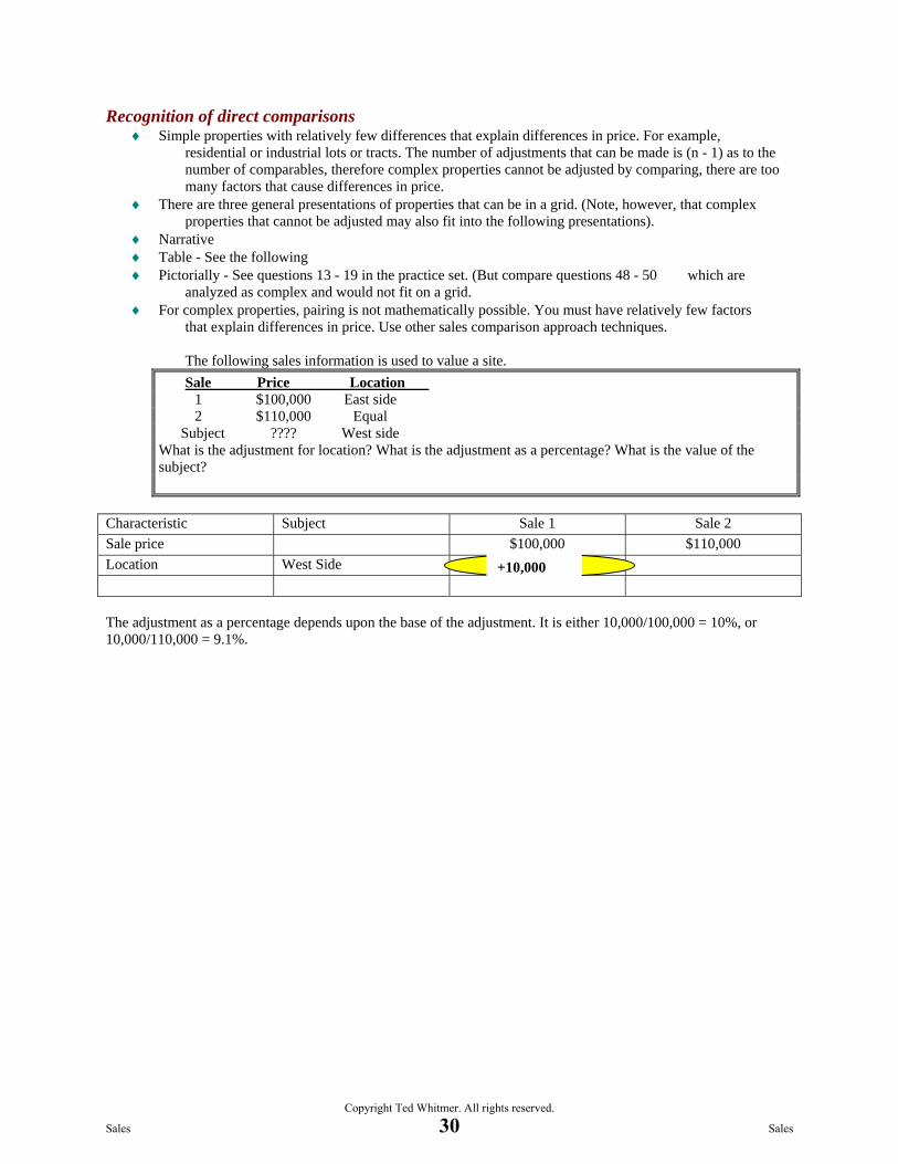
that explain differences in price. Use other sales comparison approach techniques. The following sales information is used to value a site.

Sale Price Location 1 $100,000 East side 2 $110,000 Equal Subject ???? West side What is the adjustment for location? What is the adjustment as a percentage? What is the value of the subject?

Characteristic Subject Sale 1 Sale 2 Sale price $100,000 $110,000 Location West Side The adjustment as a percentage depends upon the base of the adjustment. It is either 10,000/100,000 = 10%, or 10,000/110,000 = 9.1%.

+10,000

Sales


30 Sales

The following sales information is used to value a site. Sale Price Location Size (SF) 1 $120,000 Good 2,000 2 $110,000 Good 1,800 3 $120,000 Average 2,200 Subject ???? Average 1,900 What is each adjustment? What is the value of the subject?

Setup: You will need number of sales + 3 for the number of columns. Circle the differences between the subject and comparables. Do not put any information in a cell when the subject and comparable are equal. Put notes in the upper right hand corner. Matching circles do not necessary mean the comparables are alike. For example, all comparables are circled for size differences between the comparables and subject, but the comparables are all different sizes.

Characteristic Subject Sale 1 Sale 2 Sale 3 Price $120,000 $110,000 $120,000 Location Average

Good

-10,000 Good

-10,000

Size 1,900 sf 2,000 sf -5,000

1,800 sf +5,000

2,200 sf -15,000

Sales 1 & 2 Sales 2 & 3

Size Location

115,000

105,000

115,000

105,000

105,000

Compare sale 1 and sale 2 for size. 200 sf resulted in a difference of $10,000 or $50 psf and bigger is better. Therefore, all properties bigger than the subject should have a minus sign inserted and those smaller should have a positive sign. Then the adjustment is on the basis of $50 psf times the difference in the sale and the 1,900 sf of the subject. After the size is adjusted, use sales one and two versus sale 3 to adjust for location.

Sales


31 Sales

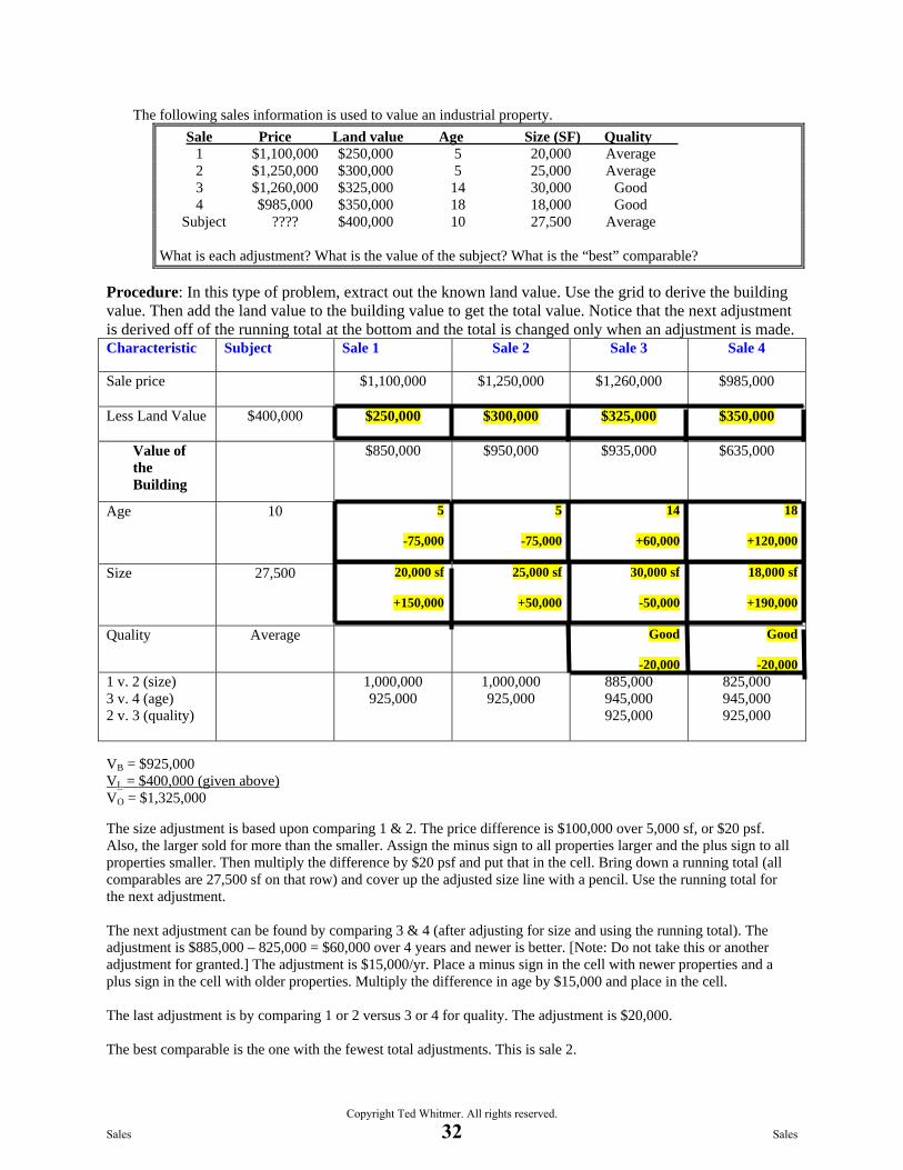
The following sales information is used to value an industrial property. Sale Price Land value Age Size (SF) Quality 1 $1,100,000 $250,000 5 20,000 Average 2 $1,250,000 $300,000 5 25,000 Average 3 $1,260,000 $325,000 14 30,000 Good 4 $985,000 $350,000 18 18,000 Good Subject ???? $400,000 10 27,500 Average What is each adjustment? What is the value of the subject? What is the “best” comparable?

Procedure: In this type of problem, extract out the known land value. Use the grid to derive the building value. Then add the land value to the building value to get the total value. Notice that the next adjustment is derived off of the running total at the bottom and the total is changed only when an adjustment is made. Characteristic Subject Sale 1 Sale 2 Sale 3 Sale 4

Sale price

$1,100,000 $1,250,000 $1,260,000 $985,000

Less Land Value $400,000

$250,000 $300,000 $325,000 $350,000

Value of the Building

$850,000

$950,000

$935,000 $635,000

Age

10 5

-75,000

5

-75,000

14

+60,000

18

+120,000

Size

27,500 20,000 sf

+150,000

25,000 sf

+50,000

30,000 sf

-50,000

18,000 sf

+190,000

Quality

Average Good

-20,000

Good

-20,000 1 v. 2 (size) 3 v. 4 (age) 2 v. 3 (quality)

1,000,000 925,000

1,000,000 925,000

885,000 945,000 925,000

825,000 945,000 925,000

VB = $925,000 VL = $400,000 (given above) VO = $1,325,000 The size adjustment is based upon comparing 1 & 2. The price difference is $100,000 over 5,000 sf, or $20 psf. Also, the larger sold for more than the smaller. Assign the minus sign to all properties larger and the plus sign to all properties smaller. Then multiply the difference by $20 psf and put that in the cell. Bring down a running total (all comparables are 27,500 sf on that row) and cover up the adjusted size line with a pencil. Use the running total for the next adjustment. The next adjustment can be found by comparing 3 & 4 (after adjusting for size and using the running total). The adjustment is $885,000 – 825,000 = $60,000 over 4 years and newer is better. [Note: Do not take this or another adjustment for granted.] The adjustment is $15,000/yr. Place a minus sign in the cell with newer properties and a plus sign in the cell with older properties. Multiply the difference in age by $15,000 and place in the cell. The last adjustment is by comparing 1 or 2 versus 3 or 4 for quality. The adjustment is $20,000. The best comparable is the one with the fewest total adjustments. This is sale 2.

Sales


32 Sales

The following sales information is used to value a retail site

Sale Price psf Size Traffic Shape Utilities Corner 1 $10.50 Optimal 20,000 cars Regular No Yes 2 $9.50 Over 20,000 cars Regular No Yes 3 $9.00 Over 15,000 cars Regular Yes Yes 4 $11.75 Optimal 20,000 cars Regular Yes Yes 5 $9.75 Optimal 20,000 cars Irregular Yes No 6 $5.50 Over 15,000 cars Regular Yes No Subject ???? Over 20,000 cars Regular Yes No

• Sale 5 had an old gas station that was removed shortly after the sale for $.50 psf of land area by the buyer. The subject and all other comps are vacant. • The subject and sale 4 needed approximately 25¢ psf of fill because of low areas. None of the others need fill.

Characteristic Subject Sale 1 Sale 2 Sale 3 Sale 4 Sale 5 Sale 6 Sale price $10.50 $9.50 $9.00 $11.75 $9.75 $5.50 Improvements

None +.50

Fill

Needs -.25 -.25 -.25 -.25 -.25

Adjusted Price $10.25 $9.25 $8.75 $11.75 $10.00 $5.25 Size

Over -1 -1 -1

Traffic

20,000 +2 +2

Shape

Regular -1.75

Utilities

Yes +1.50 +1.50

Corner

No -3.50 -3.50 -3.50 -3.50

1 v. 2 (size) 3 v. 4 (traffic) 5 v. 6 (shape) 2 v. 3 (util.) 4 v. 5 (corner)

9.25

10.75 7.25

9.25

10.75 7.25

8.75 10.75

7.25

10.75

7.25

9.00

7.25

5.25 7.25

Notes: There are no notes in the right hand corner because all adjustments are “either-or-adjustments.” The comparable is either equal to the subject or is one other difference. Also, the order in this grid just happens to be 1 & 2, then 3 & 4, etc. and from one row down to the next. This is not necessarily the case and there is absolutely no order of adjustments in a grid because the adjustments are all dollar adjustments and there are no percentage adjustments that would make the order matter. 10. Capitalization of rent differences

Sales


33 Sales

Qualitative 1. Relative comparison analysis - Use of inferior, superior, without quantifying. Often the use of “-” and

“+” signs are used in place of inferior or superior. This method has most applicability when ♦ A property is complex and has many adjustment features ♦ The adjustments cannot be quantified ♦ The subject value can be “bracketed” by the reasonable analysis of the comparable prices. For example, “the

indicated range of value is $5.00 psf to $12.00 psf for 10 sales. The subject is superior to all but one sale ($12.00 psf). However, the other sales overall support the validity of this sale as arms length, etc. and the subject is demonstrably superior to the other sales. Therefore, the value of the subject is towards the upper end of the range.”

♦ The direction of the adjustments can be reasonably argued. Although not quantifiable, the direction of adjustment (the comparable being superior means subtract and the comparable being inferior means add) should be reasonably established.

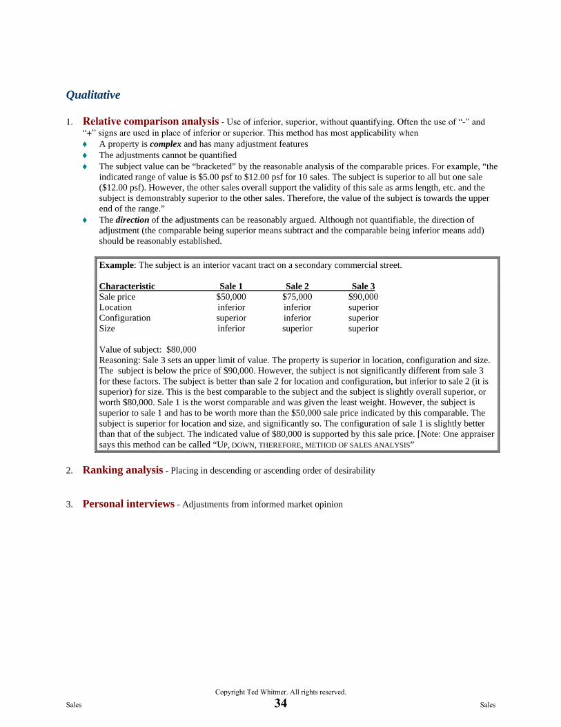
Example: The subject is an interior vacant tract on a secondary commercial street. Characteristic Sale 1 Sale 2 Sale 3 Sale price $50,000 $75,000 $90,000 Location inferior inferior superior Configuration superior inferior superior Size inferior superior superior Value of subject: $80,000 Reasoning: Sale 3 sets an upper limit of value. The property is superior in location, configuration and size. The subject is below the price of $90,000. However, the subject is not significantly different from sale 3 for these factors. The subject is better than sale 2 for location and configuration, but inferior to sale 2 (it is superior) for size. This is the best comparable to the subject and the subject is slightly overall superior, or worth $80,000. Sale 1 is the worst comparable and was given the least weight. However, the subject is superior to sale 1 and has to be worth more than the $50,000 sale price indicated by this comparable. The subject is superior for location and size, and significantly so. The configuration of sale 1 is slightly better than that of the subject. The indicated value of $80,000 is supported by this sale price. [Note: One appraiser says this method can be called “UP, DOWN, THEREFORE, METHOD OF SALES ANALYSIS”

2. Ranking analysis - Placing in descending or ascending order of desirability 3. Personal interviews - Adjustments from informed market opinion

Sales


34 Sales

P blProblem

• What is worth • Answer 1: They are

worth the same, more money a commercial retail building on the best

worth the same, only the land values are different.

• Answer 2: The on the best street in a large city, or the identical

Answer 2: The building on the better site is worth more than the building on the

building on a street with lower land values?

glesser site.

• Answer 3: The building on the values?

Assume the highest & best

building on the better site is worth less than the building on the lesser site because highest & best

use of both is the developed use.

the economic life is less.

Sales


35 Sales


Sales


36 Sales

Chapter 5 Condemnation

The federal concept of condemnation is to appraise the before, as though the governmental improvements will not be made. This is generally not an “as is” value because the influence of the improvements is not considered in the before valuation. The after value is appraised in a partial taking as though the improvements are already in place and the partial taking is completed. The compensation recommendation is based upon subtracting the after value from the before value. The appraisal of the before is the appraisal of the highest and best use of the property as though the government is not going to build the “project” and the appraisal of the after is under the highest and best use of the property as though the part taken is taken and the project is in place. The part taken is valued on the unit value before. For example, if the land is worth $2.00 psf before and $3.00 psf after, the payment of land taken is on the basis of $2.00 psf. Damages are loss in value to the after as a result of the taking. For example, if improvements are worth $50,000 before, but only $40,000 after, the damages are $10,000. It is common to have damages to the improvements when the land value increases to a higher and better use. This is because it is not likely the improvements would represent a use consistent with the higher use. Therefore, there would be special benefits to the land and damages to the improvements. If enough of a difference in highest and developed use, the improvements could become and interim use or in need of demolition. The theory of “consistent use” must be followed both in the before and after valuation. The land is valued under its highest and best use and the improvements their contribution to the highest and best use of the land. If the result of before minus after is negative or zero, then there is no compensation recommendation for the owner. In the federal concept, the owner of a property may be paid nothing if the property has increased in value as a result of the governmental improvements. However, in the federal concept general benefits cannot be used to offset special benefits. General benefits are an increase in value to the community as a whole and cannot be used to offset the damages to the after or the part taken. Special benefits are the increase that is attributable to the subject as a result of the influence of the project. Special benefits can be used to offset damages and the part taken. If the special benefits exceed the part taken and damages, there is no recommendation of compensation. General benefits are “those that arise from the fulfillment of the public object which justified the taking”, and special benefits “are those which arise from the peculiar relation of the land in question to the public improvement.” Special benefits are “direct and peculiar to the particular

Sales


37 Sales

property as distinguished from the incidental benefits enjoyed to a greater or less extent by the lands in the area of the improvement.” 3 Nichols on Eminent Domain, 3.d Ed., 45, Sect.8.6203. The federal concept is followed in many states. However, the state concepts often include a requirement where the property owner is at least paid for the part taken, regardless of special benefits. This is not the federal concept where a property owner may receive no payment, even with a physical taking of property. For example, assume a before value of $500,000, a taking of $50,000 and an after value of $550,000. In the federal concept there would be no payment. In many states the owner would be paid the $50,000 and would be left with a property worth $550,000. The tests of the parent tract are called “unities.” This is important to establish what to appraise and therefore what is the basis of compensation. The owner of a large tract would claim the part taken near the road is the “commercial property” while the governmental entity may claim the compensation should be based on the larger parcel that is primarily agricultural. The tests are (1) unity of use, (2) contiguity (is it adjacent), and (3) ownership. Some states, such as California ignore the unity of use and appraise the entire contiguous ownership and pay based upon the parent tract being the larger parcel. When valuing the parcel under the federal concept, one need only value the before and after. However, to determine the part taken, damages and special benefits, more calculations are necessary. Furthermore, the distinction between special and general benefits requires more than simply valuing on the basis of before and after. Additionally, some loss is not compensable such as business or intangible values, some circuity of travel, some access, noise, dust or smoke. (Although there are some cases where there may be an issue of compensability.) The appraiser does not have to determine compensability of damages, because the determination is a matter of law. However, the appraiser helps identify potential noncompensible items as well as special and general benefits. The determination of compensation could be formulized as follows. 1. Before – after = recommendation of compensation 2. Before – part – after = damages – special benefits (Note: this is the damages, net of special

benefits) 3. Before – part – after + special benefits = damages (1) Before (2) Part (3) After (4) Special

Benefits

Damages (1)–(2)-(3)+(4)

Compensation (1) – (2)

Sales


38 Sales

Problem: What is the before, after, part taken, special benefits, and damages of a property worth $400,000 if the government does not locate a sewer treatment plant adjacent to the property (land value is $2 psf x 60,000 sf)? Assume the land value will be $1.10 psf after the taking and the improvements will decrease in value 50% as a result of the sewer treatment plant. Furthermore, assume 20,000 sf of land will be taken with 3,000 square feet of asphalt on the area taken 20% depreciated with a cost new of $2.50 psf to replace. (Damages) Before Part After Special benefits Before - Part - After + Special benefit Land $120,000 40,000 44,000 0 36,000 Improvements 280,000 6,000 137,000 0 137,000 Total 400,000 46,000 181,000 0 173,000 or Income ÷ R Total BEFORE: (1) TOTAL OF $400,000 IS GIVEN (2) LAND VALUE IS $2 X 60,000 = $120,000 (3) IMPROVEMENTS ARE THE DIFFERENCE AFTER: (1) LAND: 40,000 X $1.10 = $44,000 (2) IMPROVEMENTS: ($280,000 BEFORE - 6,000) X 50% = $137,000 PART: (1) LAND: 20,000 X $2 = $40,000 (2) IMPROVEMENTS: 3,000 X $2.50 X (1 - 20%) = $6,000 NOTE: THE $280,000 INCLUDES THE $6,000 IN THE PART. WITHOUT DAMAGES THE AFTER VALUE OF THE IMPROVEMENTS WOULD BE $274,000. DAMAGES ARE 50% TO THE AFTER OR $137,000 ($274,000 X 50% DAMAGES

Sales


39 Sales

sales - ted whitmer companies sales comparison approach is every appraiser’s favorite approach...

Documents