sampling and reconstruction of analog signalshcso/ee3202_4.pdf · · 2011-12-23h. c. so page 1...

H. C. So Semester B, 2011-2012

Sampling and Reconstruction of Analog Signals

Chapter Intended Learning Outcomes:

(i) Ability to convert an analog signal to a discrete-time sequence via sampling (ii) Ability to construct an analog signal from a discrete-time sequence (iii) Understanding the conditions when a sampled signal can uniquely present its analog counterpart


Sampling

Process of converting a continuous-time signal into a

discrete-time sequence

is obtained by extracting every s where is

known as the sampling period or interval

sample at

analog

signal

discrete-time

signal Fig.4.1: Conversion of analog signal to discrete-time sequence

Relationship between and is:

(4.1)


Conceptually, conversion of to is achieved by a

continuous-time to discrete-time (CD) converter:

t n

impulse train

to sequence

conversion

CD converter

Fig.4.2: Block diagram of CD converter


A fundamental question is whether can uniquely

represent or if we can use to reconstruct

t

Fig.4.3: Different analog signals map to same sequence


But, the answer is yes when:

(1) is bandlimited such that its Fourier transform

for where is called the bandwidth

(2) Sampling period is sufficiently small Example 4.1 The continuous-time signal is used as the

input for a CD converter with the sampling period s.

Determine the resultant discrete-time signal .

According to (4.1), is

The frequency in is while that of is


Frequency Domain Representation of Sampled Signal

In the time domain, is obtained by multiplying by

the impulse train :

(4.2)

with the use of the sifting property of (2.12) Let the sampling frequency in radian be (or

in Hz). From Example 2.8:

(4.3)


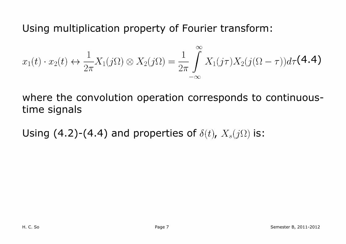
Using multiplication property of Fourier transform:

(4.4)

where the convolution operation corresponds to continuous-time signals Using (4.2)-(4.4) and properties of , is:


(4.5)

which is the sum of infinite copies of scaled by


When is chosen sufficiently large such that all copies of do not overlap, that is, or , we

can get from

......

......

Fig.4.4: for sufficiently large


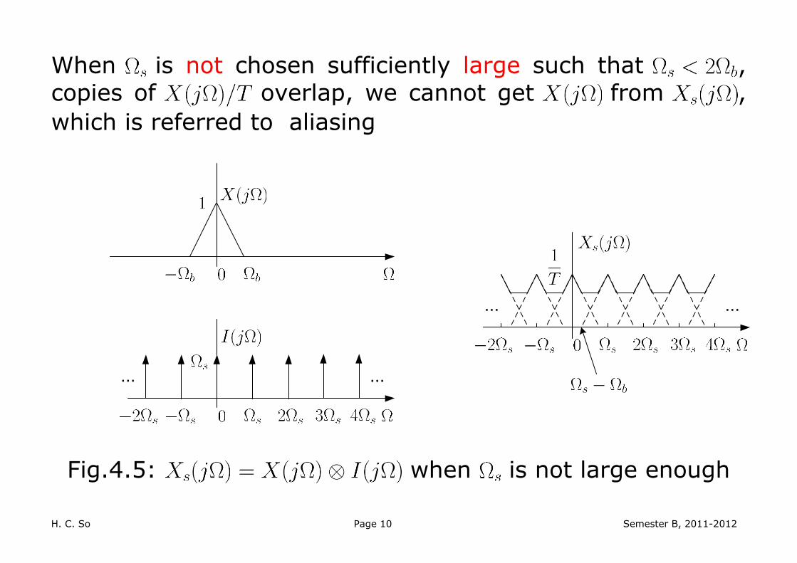
When is not chosen sufficiently large such that , copies of overlap, we cannot get from ,

which is referred to aliasing

......

......

Fig.4.5: when is not large enough


Nyquist Sampling Theorem (1928) Let be a bandlimited continuous-time signal with

(4.6)

Then is uniquely determined by its samples ,

, if

(4.7)

The bandwidth is also known as the Nyquist frequency while is called the Nyquist rate and must exceed it in order to avoid aliasing


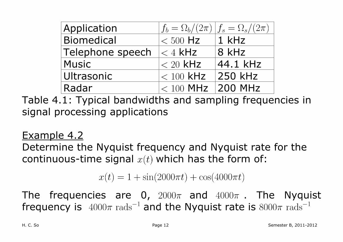
Application

Biomedical Hz 1 kHz

Telephone speech kHz 8 kHz

Music kHz 44.1 kHz

Ultrasonic kHz 250 kHz

Radar MHz 200 MHz

Table 4.1: Typical bandwidths and sampling frequencies in signal processing applications Example 4.2 Determine the Nyquist frequency and Nyquist rate for the continuous-time signal which has the form of:

The frequencies are 0, and . The Nyquist frequency is and the Nyquist rate is


......

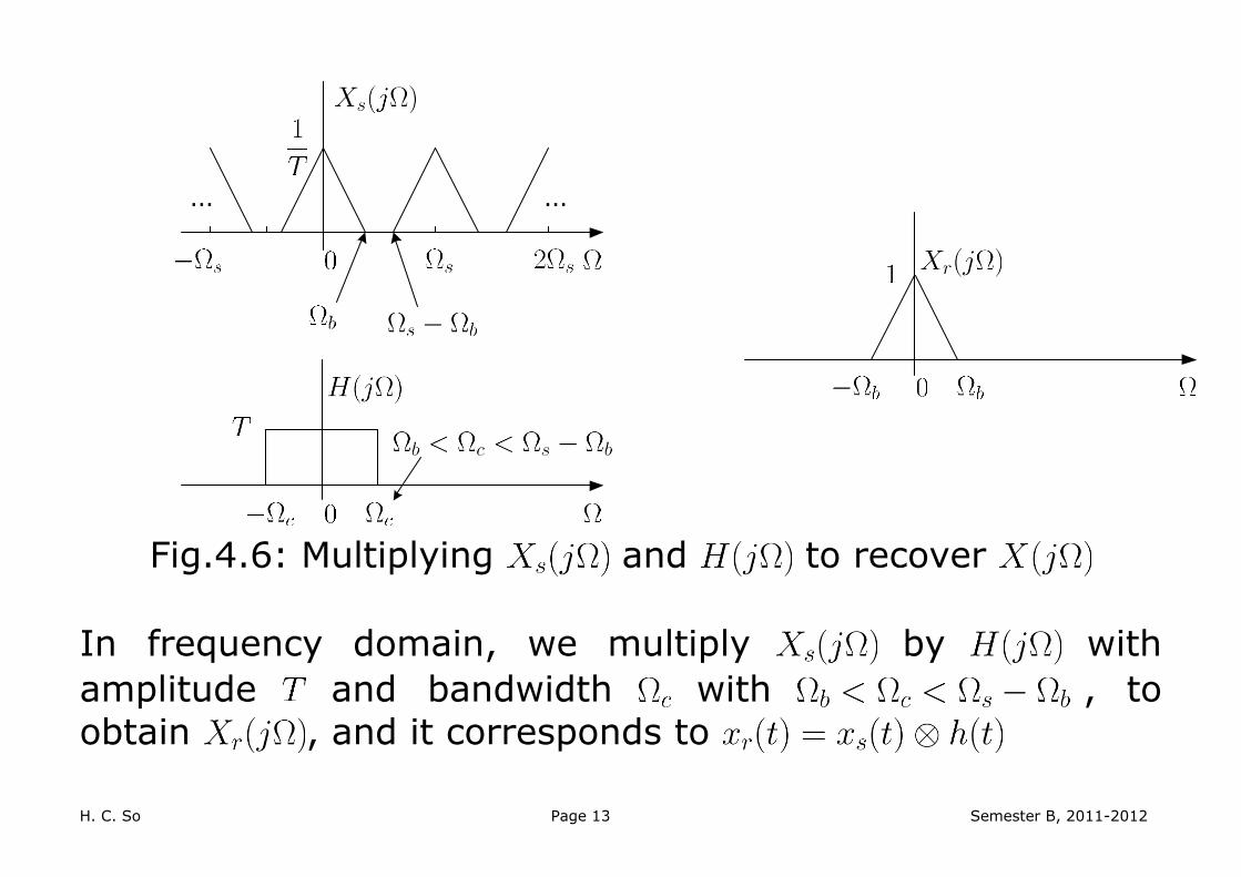
Fig.4.6: Multiplying and to recover

In frequency domain, we multiply by with

amplitude and bandwidth with , to obtain , and it corresponds to


Reconstruction

Process of transforming back to

sequence to

impulse train

conversion

DC converter

Fig.4.7: Block diagram of DC converter

From Fig.4.6, is

(4.8)

where


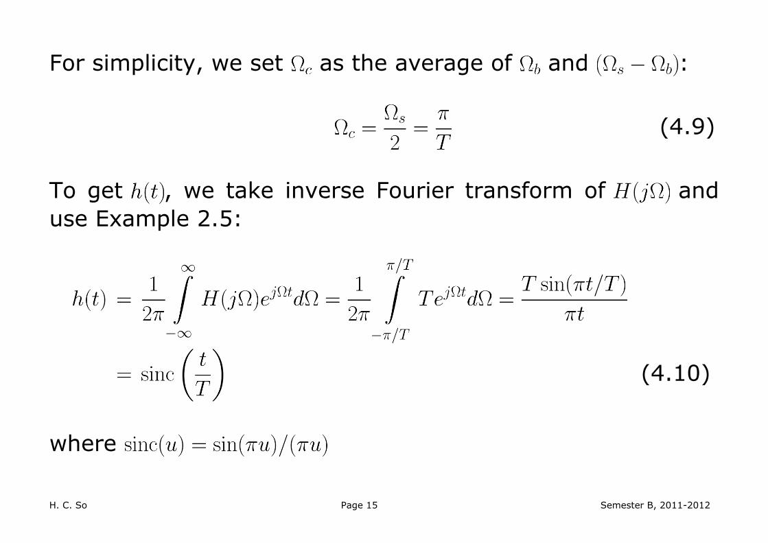
For simplicity, we set as the average of and :

(4.9)

To get , we take inverse Fourier transform of and

use Example 2.5:

(4.10)

where


Using (2.23)-(2.24), (4.2) and (2.11)-(2.12), is:

(4.11)

which holds for all real values of


The interpolation formula can be verified at :

(4.12)

It is easy to see that

(4.13)

For , we use ’s rule to obtain:

(4.14)

Substituting (4.13)-(4.14) into (4.12) yields:

(4.15)

which aligns with


Example 4.3 Given a discrete-time sequence . Generate its

time-delayed version which has the form of

where and is a positive integer. Applying (4.11)

with :

By employing a change of variable of :

Is it practical to get y[n]?


Note that when , the time-shifted signal is simply obtained by shifting the sequence by samples:

Sampling and Reconstruction in Digital Signal Processing

CD converterdigital signal

processorDC converter

Fig.4.8: Ideal digital processing of analog signal

CD converter produces a sequence from

is processed in discrete-time domain to give

DC converter creates from according to (4.11):

(4.16)


anti-aliasing

filter

digital signal

processor

digital-to-analog

converter

analog-to-digital

converter

Fig.4.9: Practical digital processing of analog signal

may not be precisely bandlimited a lowpass filter or

anti-aliasing filter is needed to process

Ideal CD converter is approximated by AD converter Not practical to generate

AD converter introduces quantization error Ideal DC converter is approximated by DA converter

because ideal reconstruction of (4.16) is impossible Not practical to perform infinite summation Not practical to have future data

and are quantized signals


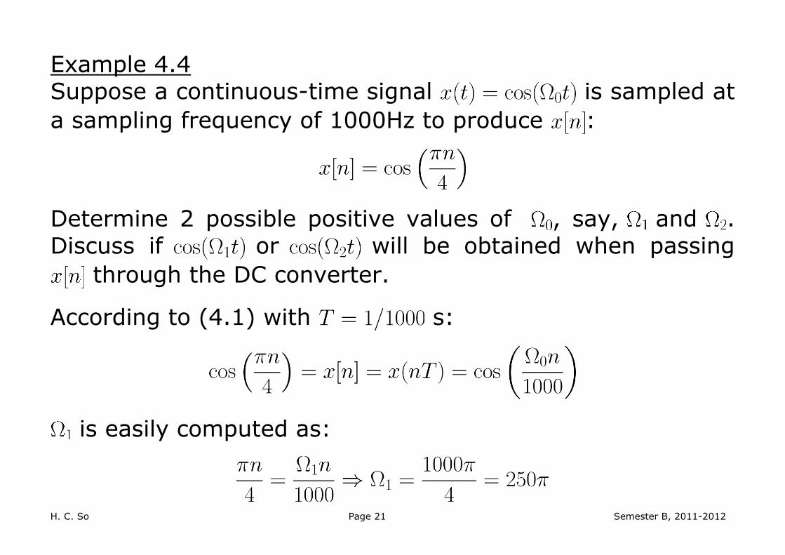
Example 4.4 Suppose a continuous-time signal is sampled at

a sampling frequency of 1000Hz to produce :

Determine 2 possible positive values of , say, and . Discuss if or will be obtained when passing

through the DC converter.

According to (4.1) with s:

is easily computed as:


can be obtained by noting the periodicity of a sinusoid:

As a result, we have:

This is illustrated using the MATLAB code:

O1=250*pi; %first frequency

O2=2250*pi; %second frequency

Ts=1/100000;%successive sample separation is 0.01T

t=0:Ts:0.02;%observation interval

x1=cos(O1.*t); %tone from first frequency

x2=cos(O2.*t); %tone from second frequency

There are 2001 samples in 0.02s and interpolating the successive points based on plot yields good approximations


0 5 10 15 20-1

-0.8

-0.6

-0.4

-0.2

0

0.2

0.4

0.6

0.8

1

n

x[n]

Fig.4.10: Discrete-time sinusoid


0 0.005 0.01 0.015 0.02-1

-0.8

-0.6

-0.4

-0.2

0

0.2

0.4

0.6

0.8

1

t

1

2

Fig.4.11: Continuous-time sinusoids


Passing through the DC converter only produces

but not

The Nyquist frequency of is and hence the

sampling frequency without aliasing is

Given Hz or , does not

correspond to

We can recover because the Nyquist frequency

and Nyquist rate for are and

Based on (4.11), is:

with s


The MATLAB code for reconstructing is:

n=-10:30; %add 20 past and future samples

x=cos(pi.*n./4);

T=1/1000; %sampling interval is 1/1000

for l=1:2000 %observed interval is [0,0.02]

t=(l-1)*T/100;%successive sample separation is 0.01T

h=sinc((t-n.*T)./T);

xr(l)=x*h.'; %approximate interpolation of (4.11)

end

We compute 2000 samples of in s

The value of each at time t is approximated as x*h.'

where the sinc vector is updated for each computation

The MATLAB program is provided as ex4_4.m


0 0.005 0.01 0.015 0.02-1

-0.8

-0.6

-0.4

-0.2

0

0.2

0.4

0.6

0.8

1

t

xr(t)

Fig.4.12: Reconstructed continuous-time sinusoid


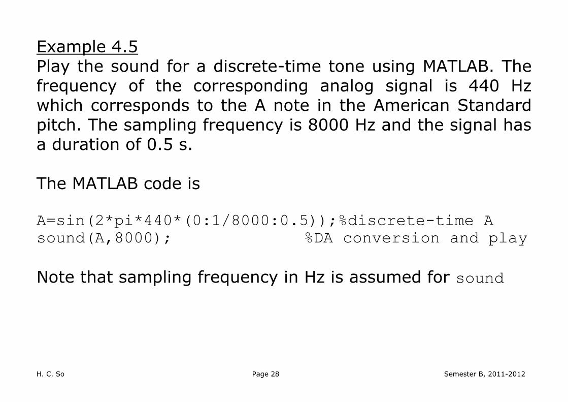
Example 4.5 Play the sound for a discrete-time tone using MATLAB. The frequency of the corresponding analog signal is 440 Hz which corresponds to the A note in the American Standard pitch. The sampling frequency is 8000 Hz and the signal has a duration of 0.5 s. The MATLAB code is A=sin(2*pi*440*(0:1/8000:0.5));%discrete-time A

sound(A,8000); %DA conversion and play

Note that sampling frequency in Hz is assumed for sound

sampling and reconstruction of analog signalshcso/ee3202_4.pdf · · 2011-12-23h. c. so page 1...

Documents