santa catarina state university udesc college of

Títu

lo

No

me

do A

uto

r

This dissertation investigates the effects of well

modeling on production forecasts for a

hydrocarbon reservoir. To carry out this work, a

program was developed, this program considers

the pressure losses over the entire length of the

well, including in the region of the production zone.

The results showed that the well model has an

expressive impact on the estimated production.

Advisor: Marcus Vinícius Canhoto Alves

Joinville, 2020

DISSERTAÇÃO DE MESTRADO

NUMERICAL MODELING OF THE COUPLED INTERACTION BETWEEN PRODUCTION WELL AND RESERVOIR

2020

R

AFA

EL JOA

QU

IM A

LVES |N

UM

ERIC

AL M

OD

ELING

OF TH

E CO

UP

LED

INTER

AC

TION

BETW

EEN P

RO

DU

CTIO

N W

ELL AN

D R

ESERV

OIR

SANTA CATARINA STATE UNIVERSITY – UDESC COLLEGE OF TECHNOLOGICAL SCIENCE – CCT MECHANICAL ENGINEERING GRADUATE PROGRAM

RAFAEL JOAQUIM ALVES

JOINVILLE, 2020

RAFAEL JOAQUIM ALVES

NUMERICAL MODELING OF THE COUPLED INTERACTION BETWEEN

PRODUCTION WELL AND RESERVOIR

Master thesis submitted to the Mechanical Engineering

Department at the College of Technological Science of

Santa Catarina State University in fullfillmet of the partial

requirement for the Master`s degree in Mechanical

Engineering.

Advisor: Marcus Vinícius Canhoto Alves

JOINVILLE - SC

2020

Dedico este trabalho a minha mãe Jocélia Fátima

Alves e aos meus tios Joel e Joélia por todos os

tipos de apoio dados ao longo da minha vida.

ACKNOWLEDGMENT

I would like to thank my entire Family for helping me to carry out this project in all of

its aspects.

I would like to thank my friends for their overall support.

I would like to thank Prof. Marcus Vinicius Canhoto Alves, for his guidance, advice,

partnership, patience and for suggesting me a very interesting subject of study. It was an

honor to work with him for five years.

I am grateful to the State University of Santa Catarina–UDESC and the Department of

Mechanical Engineering for the educational opportunity and the Department of Petroleum

Engineering for some reference books.

I thank Cleomir Waiczyk for the support regarding administrative issues.

A special word of gratitude is due to the Coordination for the Improvement of Higher

Education Personnel – CAPES for the Master Scholarship at UDESC (CAPES 001 grant

program).

Also, I express my thanks to the Nacional Council of Scientific and Technological

Development for funding this work and for the overall support to our laboratory (CNPq

43382020187 grant program).

Finally, I would like to acknowledge with gratitude the Santa Catarina State Research

Foundation – FAPESC for also funding this work and for the overall support to our laboratory

(FAPESC 2019TR000779 and FAPESC 2019TR000783 grant programs).

RESUMO

A simulação acoplada de poços e reservatórios é de grande importância para que se possa

obter resultados confiáveis de produção em campos de hidrocarbonetos; neste sentido, este

trabalho apresenta os passos para o desenvolvimento de um simulador de acoplamento

incompletamente implícito. Uma apresentação do sistema físico a ser simulado, bem como de

trabalhos anteriores que abordaram a solução acoplada deste sistema é realizada. Para o

desenvolvimento do simulador principal foram acoplados um simulador de reservatório, um

simulador de escoamentos bifásicos permanentes que não considera influxos radias e um

simulador que representa a região do poço que recebe influxo do reservatório também de

regime permanente; estes três simuladores foram acoplados de 4 maneiras diferentes. Além

deste simulador de acoplamento principal, em que o reservatório é simulado de maneira

transiente utilizando o método de volumes finitos, foi desenvolvido um simulador secundário

que resolve o reservatório utilizando a equação do balanço de massa. Os primeiros resultados

obtidos estavam relacionados à possibilidade de se adaptar uma correlação bifásica que

originalmente não considerava influxos radiais para um cenário com esse tipo de influxo.

Esses resultados mostraram que em poços horizontais, os números obtidos para a perda de

pressão dentro do poço foram bastante diferentes utilizando a correlação antes e depois das

modificações; além disso, os resultados depois das modificações se aproximaram mais dos

números de referência obtidos com uma correlação originalmente desenvolvida para

considerar os influxos do reservatório. Os resultados obtidos com o simulador de reservatório

discretizado foram bastante satisfatórios, indicando que o simulador acoplado foi

efetivamente desenvolvido. A comparação dos quatros métodos de acoplamento

implementados apontou que os métodos em que os três simuladores iteram em apenas um

laço iterativo são menos suscetíveis a falhas, mas necessitam mais iterações quando

comparados com os métodos que utilizam dois laços. Além disso, o trabalho utilizou um

simulador de poço que permitia o uso de 4 correlações para o poço sem influxo e de 2 duas

para a região do poço sob influxo do reservatório; os números obtidos para a perda de

pressão utilizando cada um desses modelos foram comparados, e as comparações mostraram

que os resultados obtidos para a produção variaram muito de acordo com o modelo utilizado

na região sem influxo. Em função do menor comprimento, a correlação utilizada na região do

poço com influxo foi pouco influente. Finalmente o simulador acoplado foi utilizado para

simular situações similares de produção com raios diferentes; os resultados indicam que os

impacto dos raios, ainda que sempre tenham resultado em maior produção por surgência

quando o menor raio foi utilizado, podem variar muito de acordo com a correlação utilizada.

Desse modo, os resultados finais obtidos foram bastante satisfatórios, trabalhos futuros devem

focar em aproveitar a estrutura desenvolvida para simulações que se aproximem de situações

mais específicas de produção, como prever formação de carga de líquido no poço.

Palavras-chave: Acoplamento poço-reservatóro. Correlações de fluxo multifásicas. Sistema

de produção de petróleo.

ABSTRACT

The coupled simulation of wells and reservoirs is of great importance in order to obtain

reliable production results in hydrocarbon fields; in this sense, this work presents the steps for

the development of an incompletely implicit coupling simulator. A presentation of the

physical system to be simulated, as well as of previous works that addressed the coupled

solution of this system is made. For the development of a main simulator, all these simulators

were coupled: a reservoir simulator, a simulator of steady-state two-phase flows that does not

consider radial inflows and a steady-state simulator that handles the region of the well that

permanently receives influx from the reservoir; these three simulators were coupled in 4

ways. In addition to this main coupling simulator, in which a reservoir is simulated in a

transient way using the finite volume method, a secondary simulator was developed to

simulate the reservoir using the mass balance equation. The first results obtained were related

to the possibility of adapting a two-phase correlation that originally did not consider radial

inflows for a scenario with this type of influx. These results showed that in horizontal wells,

the pressure loss figures in the well can vary a lot if the correlation is used before or after

the modifications; in addition, the results after the modifications were closer to the reference

numbers obtained with a correlation originally developed to consider the inflows from the

reservoir. The outcome obtained with the discretized reservoir simulator was quite

satisfactory, indicating that the coupled simulator was effectively developed. The comparison

of the four coupling methods implemented showed that the methods in which the three

simulators iterate in only one iterative loop are less susceptible to failures but require more

iterations when compared to the methods that use two loops. Besides that, this work used a

well simulator that allowed the use of 4 correlations for the well region without inflow and

two correlations for the well region under inflow from the reservoir; the figures obtained for

the pressure loss using each one of these models were compared, and the comparisons showed

that production results varied a lot in line with the model applied in the region without

inflow. In the face of a shorter length, the correlation used in the region of the well with

inflow was not very influential. Finally, the coupled simulator was used to simulate similar

situations of production with different radii; the results indicate that the impact of the radius,

despite having always resulted in greater production due to the reservoir natural energy when

the smallest radius was used, can vary a lot according to the correlation used. In the face of

the satisfactory end results achieved, future works should focus on taking advantage of the

structure developed for simulations that approach more specific production situations, like

predicting the formation of liquid loads in the well.

Keywords: Well-reservoir coupling. Multiphase flow correlations. Petroleum Production

System.

LIST OF FIGURES

Figure 1.1 - Schematic representation of a production system…………………………..…...23

Figure 1.2 - Division of the model utilized by this work…………………………………..…25

Figure 1.3 - Representation of two-phase flow patterns for vertical flow………………...….26

Figure 1.4 - Well Completion with Production Liner…………………………………..…….27

Figure 1.5 - Nodal analysis for BHP using IPR and TPR………………………………….....29

Figure 2.1 - Time and space scales for well and reservoir events…………………..………...32

Figure 2.2 – Connections between chapters and results obtained…………………..………...36

Figure 3.1 - BHP determination algorithm…………………………………………………...38

Figure 4.1 - Algorithm utilized to determine wellbore pressures to match BHP and reservoir

inflows ………………………………….…………………………………………………….42

Figure 4.2 - Representation of where values are taken from to calculate the pressure

derivative………………………………………………………………………………..…….43

Figure 4.3 - Representation of control volume for flow with inflow through perforations ...…...46

Figure 4.4 - Wave formation that leads to intermittent flow……………………………..…...50

Figure 4.5 - Slug liquid holdup isolines (dashed lines are just illustrative) ………………….51

Figure 4.6 - Instability of a solitary wave ………………………………………………...….56

Figure 4.7 - Calculations to solve stratified regime …………………………………….……63

Figure 4.8 - Calculations to solve annular regime ……………………………………..…….66

Figure 5.1 - Point distribution around a central point P – r and z…………………….………76

Figure 5.2 - Point distribution around a central point P – θ…………………………….…….76

Figure 5.3 - Representation of a cylindrical grid……………………………………..………76

Figure 5.4 - Matrix of derivatives for a 1x1x3 grid – each line represents three matrix lines

𝛼 = 𝑜,𝑤, 𝑔……………………………………………………………………………………91

Figure 5.5 - Plan View of Reservoir Physical Model utilized to apply the Permadi Model….93

Figure 6.1 - Algorithm for Coupling Method 1………………………………………...…….96

Figure 6.2 - Algorithm for Coupling Method 2………………………………………...…….97

Figure 6.3 - Algorithm for Coupling Method 3……………………...……………………….98

Figure 6.4 - Algorithm for Coupling Method 4…………………………………………...….99

Figure 6.5 - Algorithm for horizontal coupling…………………………………………......100

Figure 6.6 - Detailed algorithm for an estimate of BHP…………………………………….102

Figure 6.7 - Detailed algorithm for an estimate of PWB and to determine Wellbore Error...103

Figure 7.1 - Horizontal well positions nomenclature………………………………...……...104

Figure 7.2 - Pressure Drop in Wellbore between heel and toe for Case 1 ……….………..….106

Figure 7.3 - Total Oil Flow Rate for Case 1 .............................................……….………..….106

Figure 7.4 - Liquid holdup in Wellbore for the first depletion step - Case 1……...………...107

Figure 7.5 - Pressure Drop in Wellbore between heel and toe for Case 2 .……………………108

Figure 7.6 - Liquid holdup in Wellbore for the first depletion step - Case 2……...………...108

Figure 7.7 - Pressure Drop in Wellbore between heel and toe for Case 9 ...……………..…109

Figure 7.8 - Liquid holdup in Wellbore for the first depletion step - Case 9 ..………………...109

Figure 7.9 - Pressure Drop in Wellbore between heel and toe for Case 16 ………………...110

Figure 7.10 - Liquid holdup in wellbore for the last depletion step - Case 16 ...……….…...111

Figure 7.11 - Pressure in wellbore for the last depletion step - Case 16 ..…………………..111

Figure 7.12 - Pressure Drop in Wellbore between heel and toe for Case 16 ....…………….112

Figure 7.13 - Total Oil Flow Rate for Case 17 .........................................……….………..….112

Figure 7.14 - Liquid holdup in wellbore for the first depletion step - Case 17……..……….113

Figure 7.15 - Pressure in wellbore for the first depletion step - Case 17……..…………….113

Figure 7.16 - Total Pressure Drop estimated for each depletion step in every simulation

case…………………………………………………………………………………………..114

Figure 8.1 - Iterations of coupling methods for Case 1 every 50 time steps………………..118

Figure 8.2 - Oil Flow Rate for Case 1……………………………………………………….118

Figure 8.3 - Iterations of coupling methods for Case 2 every 50 time steps………………...119




Figure 8.7 - Oil Flow Rate for Case 5……………………………………………………….122

Figure 8.8 - Iterations of coupling methods for Case 6 every 50 time steps……………...…123


Figure 8.10 - Oil Flow Rate for simulations 1 to 4………………………………………….127

Figure 8.11 - Cumulative oil production for simulations 1 to 4.….......................………….127

Figure 8.12 - BHP for simulations 1 to 4……………………………………………………128

Figure 8.13 - GOR for simulations 1 to 4…………………………………………………...129

Figure 8.14 - Oil Flow Rate for simulations 25 to 28………………………………….……130

Figure 8.15 - BHP for simulations 25 to 28…………………………………………………130

Figure 8.16 - Oil Flow Rate for simulations 21 to 24………………………………….……131

Figure 8.17 - Oil Flow Rate for simulations 29 and 61……………………………….…….132

Figure 8.18 - BHP for simulations 20 and 52……………………………………………….133

Figure 8.19 - BHP for simulations of line 5 of Table 8.4……………………………...……135

Figure 8.20 - Oil Flow Rate for simulations of line 9 of Table 8.4…………………………135

Figure A.1 – Algorithm to Lockhart-Martinelli Solution…………………………..……….153

LIST OF TABLES

Table 4.1 - Effects of inflow and outflow over the wall shear stress ….………………...…...45

Table 5.1 - Factors obtained from the substitution of pressures derivatives by Taylor First

Order Approximation …………………………….………...…………………………...……79

Table 5.2 - Groups of properties and approximation at boundaries ………………………….80

Table 5.3 - Weight of 𝑋 at each boundary ……….……………………………………….….80

Table 5.4 - Derivatives obtained using operator 𝑑{𝐹}𝝋, 𝜑 = 𝑝𝑜 , 𝑆𝑤, 𝑇…………….…..…….84

Table 5.5 - Derivatives of 𝜆1 with respect to the 𝜑 ………………………..………………...84

Table 5.6 - Derivatives of 𝜆2 with respect to the 𝜑 ….………………………………………84

Table 5.7 - Derivatives of 𝜆3 and 𝜆4 with respect to the 𝜑, 𝛽 = 𝑜 …………………….…….85

Table 5.8 - Derivatives associated with reservoir state ………………………………….…...85

Table 5.9 - Units utilized in the reservoir simulator……...………………………………..…89

Table 7.1 – Simulation Cases………………………...……………………………………...105

Table 8.1 – Coupling methods results for 8 simulation cases……….….……………..…….116

Table 8.2 – Simulations using Ouyang Homogeneous Wellbore Correlation …………...…125

Table 8.3 – Simulations using Beggs & Brill Modified Wellbore Correlation

...…………………...……………………………………………………………………...…126

Table 8.4 – Production results with two well radius ………...……….……………………..134

Table B.1 - Characterization of Reservoir 1 ……….………………………………...….….154

Table B.2 – Characterization of Reservoir 2 …………………………………………….….154

Table B.3 – Wellbore Permanent Characteristics………………………......………….……155

Table B.4 – Solution GOR ……………………. ………...……………...………………….155

Table B.5 – Oil volume factor ………………………….……….….…………...………….156

Table B.6 – Gas volume factor ………………………………………………………….….156

Table B.7 – Oil density…………………………………………………......…….…………157

Table B.8 – Oil viscosity ………………………….………...……….……...………………157

Table C.1 - Reservoir basic characteristics…………………………………….……...…….159

Table C.2 – Reservoir grid in vertical direction …………………………………………….160

Table C.3 – Constants for relative permeabilities calculations ……………......…..……..…161

Table C.4 – Constants for water volume factor calculation.…...…………...……………….162

Table C.5 – Constants for water density calculation.….………………………...……….....162

Table C.6 – Auxiliary values for oil viscosity calculation ………………………………….163

Table C.7 – Constants for gas viscosity calculation ………………………....……………..164

LIST OF SYMBOLS

𝑎 Expansion factor to radial grid distribution

𝐴 Area

𝐴𝜔,𝑝 Factor associated with FVM integration

𝐴𝜏,𝑝 Geometrical factor associated with orientation of boundary of point 𝑝

𝐴𝑓𝑎𝑛 Coefficient for Fanning Factor calculation

𝐵 Formation volume factor

𝐵𝑜 Bond Number

𝐵𝑓𝑎𝑛 Coefficient for Fanning Factor calculation

𝐵𝐻𝑃 Bottom-hole pressure

𝑐0 Drift-flux model coefficient

𝐶1 Unit correction constant



𝐶𝑓𝑎𝑛 Coefficient for Fanning Factor calculation

𝐶𝐼𝐷 Drag coefficient

𝐶𝑙𝐵&𝐵 Volumetric fraction of liquid in main inflow

𝐶𝐼𝑙 Volumetric fraction of liquid in radial inflow

𝐶𝑝 Heat capacity

𝑐𝑤 Drift-flux model coefficient

𝐷 Well diameter

𝐷𝑐𝑟𝑖𝑡 Critical diameter value

𝐷𝑚𝑎𝑥 Maximum diameter of a bubble in the flow

𝐷𝑃𝑊𝐵 Difference of pressure between the mean pressure of the reservoir and the pressure at

the well heel

𝐸𝑙 Liquid hold-up

𝐸𝑙𝑠 Liquid hold-up in the slug

𝑓 Friction factor

𝐹𝑒 Volumetric fraction of liquid entrained in gas core

𝐹𝑟 Froude number

𝑔 Acceleration of gravity

𝐺 Mass flow rate

𝐺𝑂𝑅 Production gas-oil ratio

𝐺𝑝 Cumulative gas production

ℎ Enthalpy

ℎ𝑙 Liquid height

ℎ𝑔 Gas height

𝐽ℎ Productivity index of a horizontal well

𝑘 Relative permeability

𝐾 Absolute permeability

𝐿 Wellbore coordinate from bottom to top (wellbore) or wellbore length (reservoir)

𝑚 Number of points in radial direction

𝑁 Initial oil-in-place

𝑁𝑝 Cumulative oil production

𝑝 Pressure

𝑃 Perimeter

𝑃𝑠𝑢𝑟𝑓 Wellhead pressure (Top hole Presure)

𝑃𝑊𝐵 Wellbore pressure

𝑝𝛼,𝜏 Pressure of phase 𝛼 in a neighbor point of point 𝑝

𝑝𝛼,𝑝 Pressure of phase 𝛼 in a point 𝑝

𝑄 Total flow rate in the well

𝑞𝐼 Inflow rate per length

𝑅 Radial position

𝑅𝑎𝑓 Ratio of acceleration and frictional pressure gradients

𝑅𝑑𝑎 Ratio of directional and acceleration pressure gradients

𝑅𝑒 Reynolds number

𝑟𝑒 Reservoir external radius

𝑅𝑒𝑤 Wall Reynolds number

𝑅𝑔𝑓 Ratio of gravitational and frictional pressure gradients

𝑟𝑟𝑒𝑠𝑒𝑟𝑣𝑜𝑖𝑟 Reservoir external radius

𝑅𝑠𝛽 Ratio of phase 𝛼 dissolved in phase 𝛽

𝑟 Reservoir radial coordinate

𝑟𝑤 Wellbore radius

𝑟𝑤𝑒𝑙𝑙𝑏𝑜𝑟𝑒 Wellbore radius

𝑆 Saturation

𝑆𝐵&𝐵 Beggs and Brill model coefficient

𝑇 Temperature (well), derivation variable according to gas presence at a grid

point(reservoir)

𝑡 Time

𝑇𝐻𝑃 Top hole pressure

𝑡𝑚𝑖𝑛 Reservoir simulation time in minutes

𝑇𝑆 Time step

𝑈 Velocity

𝑣 Fluid velocity

𝑥 Well coordinate (from bottom to top)

𝑋𝑒 Reservoir width

𝑋𝑝𝑏 Boolean value that is dependent on the presence of gas at a point of the grid

𝑦 Beggs and Brill model coefficient

𝑌𝑒 Reservoir length parallel to horizontal well axis

𝑧 Reservoir depth coordinate

𝑍 Vertical position

𝛿 Film thickness

Δ𝑡 Time step length

Δ𝑍𝑝,𝜏 Absolute value of depth distance between point 𝑝 and 𝜏

𝜖 Roughness

𝜂 Joule-Thompson coefficient for well equations and hydraulic diffusivity for reservoir

equations

𝜃 Well inclination or reservoir angular coordinate

Θ Angular position

𝜗(𝜏) Boolean function, adjust gravity effects according boundary direction

𝜅 Constant of Hinze Model to determine the maximum possible diameter of a bubble in

the flow

Κ Coefficient of Hinze Model to determine the maximum possible diameter of a bubble

in the flow

𝜆 Gas, liquid densities ratio

𝜇 Viscosity

𝜌 Density

𝜎 Surface tension

𝜏𝑤 Shear Stress in pipe wall

𝛾 Inflow angle

𝜙 Rock porosity

Φ Coefficient for production forecast

X(𝜏) Weight factor at boundary 𝜏

𝜔𝑜𝑢 Weight to estimate acceleration term in Ouyang Model

(𝐾𝜔)𝑝,𝜏 Absolute permeability in boundary between points 𝑝 and 𝜏

(𝑅𝑒𝑠𝛼)𝑝 Numerical residue for application of Newton-Raphson Method in equation of

phase 𝛼 in a point 𝑝

[ (𝜆1)𝛼]𝑝,𝜏 Transmissibility of phase 𝛼 over absolute permeability in boundary between

points 𝑝 and 𝜏

[ (𝜆3)𝛽]𝑝,𝜏 [ (𝜆1)𝛽]𝑝,𝜏

multiplied by 𝑅𝑠𝛽 in boundary between points 𝑝 and 𝜏

[ (𝜆2)𝛼]𝑝,𝜏 [ (𝜆1)𝛼 ]𝑝,𝜏 multiplied by 𝜌𝛼 in boundary between points 𝑝 and 𝜏

[ (𝜆4)𝛽]𝑝,𝜏 [ (𝜆3)𝛽]𝑝,𝜏

multiplied by 𝜌𝛽 in boundary between points 𝑝 and 𝜏

SUBSCRIPTS

0 Deepest point in wellbore

𝑎𝑣 Average during a time step

𝐵 Buoyancy (wellbore) or backward position (reservoir)

𝑏 Bubble (wellbore) or backward boundary (reservoir)

𝑐 Gas Core

𝑐𝛼 Critical of phase 𝛼

CALC Indicates a value that is estimated by the program

𝑑 Dimensioless

𝑑𝑏 Dispersed Bubbles

𝑑𝐻 Dispersed Bubbles in horizontal direction

𝑑𝑟 Drift

𝑑𝑉 Dispersed Bubbles in vertical direction

𝑒 East boundary

𝐸 East position

𝑓 Liquid Film(wellbore) or forward boundary (reservoir)

𝐹 Forward position

𝑔 Gas

ℎ Horizontal

𝑖 Indicates interfacial properties, wellbore grid position or reservoir time step

𝐼 Inflow

𝑖𝑛𝑖𝑡 Initial reservoir condition

𝑙 Liquid

𝐿 Longitudinal

𝑚 Mixture

𝑛 North boundary

𝑁 North position

𝑝 Represents one point of reservoir grid

𝑟 Radial or reservoir radial coordinate

𝑟𝑒𝑠 Reservoir

𝑠 Slip (well and wellbore) or south boundary (reservoir)

𝑆 South position

𝑡 Time

𝑇 Turbulent

𝑡𝑝 Two-phase mixture

𝑣 Vertical

𝑤 Wall(wellbore) or water (reservoir property) or west boundary (Grid related)

𝑊 West position

𝑧 Reservoir axial coordinate

𝛼 Represents the phase of fluid (oil, gas, or water)

𝛽 Represents the phase in which the phase of equation is dissolved on reservoir

simulation

𝜃 Reservoir angular coordinate

𝜔 Represents the coordinate, 𝑧, 𝜃 or 𝑟

𝜑 Represents one of three main properties in reservoir (𝑝𝑜, 𝑆𝑤 or 𝑇)

𝜏 Represents the neighbor of reservoir grid point 𝑝 in orientation 𝜏

∞ Translational

CONTENTS

1 INTRODUCTION ............................................................................................................... 23

1.1 WELL ............................................................................................................................................................. 25

1.2 WELLBORE .................................................................................................................................................. 27

1.3 RESERVOIR ................................................................................................................................................. 28

1.4 COUPLING ................................................................................................................................................... 28

1.5 OBJECTIVES ................................................................................................................................................ 30

2 REVIEW OF COUPLING METHODS ............................................................................ 31

3 WELL ................................................................................................................................... 37

3.1 WELLHEAD PRESSURE ITERATIVE ALGORITHM .......................................................................... 37

3.2 WELL PRESSURE AND TEMPERATURE INTEGRATION ................................................................ 39

3.3 WELL CORRELATIONS ............................................................................................................................ 40

4. WELLBORE ....................................................................................................................... 41

4.1 WELLBORE ALGORITHM ....................................................................................................................... 41

4.2 WELLBORE PRESSURE NUMERICAL INTEGRATION .................................................................... 42

4.3 WELLBORE MODELS ............................................................................................................................... 43 4.3.1 OUYANG SINGLE-PHASE MODEL......................................................................................................... 44 4.3.2 OUYANG MECHANISTIC MODEL ......................................................................................................... 49 4.3.2.1 Intermittent-Annular Transition ................................................................................................................ 49 4.3.2.2 Intermittent-Dispersed Bubble Transition ................................................................................................. 52 4.3.2.2.1 Creaming and Bubble Migration ............................................................................................................ 52 4.3.2.2.2 Bubble Agglomeration and Coalescence ................................................................................................ 54 4.3.2.2.3 Maximum Packing .................................................................................................................................. 55 4.3.2.3 Transition from Stratified Flow ................................................................................................................. 55 4.3.2.3 Pressure drop and hold-up calculations ..................................................................................................... 59 4.3.2.3.1 Stratified Flow Calculation ..................................................................................................................... 59 4.3.2.3.2 Annular-Mist Flow Calculation .............................................................................................................. 64 4.3.2.3.3 Intermittent Flow Calculation ................................................................................................................. 66 4.3.2.3.4 Bubble Flow Calculation ........................................................................................................................ 69 4.3.2 OUYANG HOMOGENOUS TWO-PHASE FLOW MODEL .................................................................... 70 4.3.3 BEGGS & BRILL MODIFIED FOR RADIAL INFLOW OR OUTFLOW ................................................ 72

5 RESERVOIR MODELING ................................................................................................ 75

5.1 RESERVOIR SIMULATION USING THE FINITE VOLUMES METHOD ........................................ 75

5.1.1 RESERVOIR GRID ..................................................................................................................................... 75 5.1.2 FINITE VOLUME METHOD ..................................................................................................................... 77 5.1.2.1 Boundary Conditions ................................................................................................................................. 86 5.1.2.2 Point distribution in direction r .................................................................................................................. 87 5.1.2.3 Units and Constants ................................................................................................................................... 89 5.1.2.4 Newton-Raphson Method and Matrix Solver ............................................................................................ 90

5.2 SIMPLIFIED RESERVOIR MODEL FOR COMPLEMENTARY SIMULATIONS ........................... 91 5.2.1 PERMADI MODEL FOR SEMISTEADY-STATE FLOW ........................................................................ 92 5.2.2 PRODUCTION FORECAST FROM A TWO-PHASE RESERVOIR WITH SOLUTION GAS DRIVE AS

PRODUCTION MECHANISM ............................................................................................................................ 93

6 COUPLING .......................................................................................................................... 95

6.1 COUPLING METHOD 1 ............................................................................................................................. 95

6.2 COUPLING METHOD 2 ............................................................................................................................. 96

6.3 COUPLING METHOD 3 ............................................................................................................................. 97

6.3 COUPLING METHOD 4 ............................................................................................................................. 98

6.5 COUPLING METHOD FOR HORIZONTAL WELLS .......................................................................... 100

6.6 ROOT FINDING ALGORITHMS FOR FINDING 𝑩𝑯𝑷 AND 𝑷𝑾𝑩𝟎 ................................................ 101

7 HORIZONTAL WELL SIMULATIONS ....................................................................... 104

7.1 SIMULATION CASES ............................................................................................................................... 104

7.2 RESULTS ..................................................................................................................................................... 105

8 VERTICAL WELL SIMULATIONS .............................................................................. 115

8.1 COUPLING METHODS ............................................................................................................................ 116

8.2 CORRELATIONS ....................................................................................................................................... 125 8.2.1 IMPACT OF WELL CORRELATIONS.................................................................................................... 126 8.2.2 WELLBORE CORRELATIONS IMPACT ............................................................................................... 131

8.3 WELL RADIUS ........................................................................................................................................... 133

9 CONCLUSIONS ................................................................................................................ 136

REFERENCES ..................................................................................................................... 139

APPENDIX A ........................................................................................................................ 149

A.1 LOCKHART-MARTINELLI FOR STRATIFIED FLOW .................................................................... 149

A.2 LOCKHART-MARTINELLI FOR ANNULAR FLOW ........................................................................ 150

A.3 RIDDERS’ METHOD ADAPTED TO 𝒉𝒍𝒅 AND 𝜹𝒍𝒅 CALCULATIONS............................................ 151

APPENDIX B ........................................................................................................................ 154

B.1 RESERVOIRS UTILIZED FOR HORIZONTAL WELLBORE SIMULATION ............................... 154

APPENDIX C ........................................................................................................................ 159

C.1 RESERVOIR UTILIZED FOR VERTICAL SIMULATION ................................................................ 159

C.2 ROCK AND FLUID PROPERTIES ......................................................................................................... 160

23

1 INTRODUCTION

According to BP Energy Economics (2019), if technologies, government measures and

also public opinion maintain the same trend and the same influence that they have today on

the energy field, the use of oil as an energy source will grow in absolute numbers until 2030

and will remain stable until 2040, even if oil percentage share of the energy market decreases.

In this scenario, natural gas would gain significant space, accounting for almost 85% of the

growth in energy supply, surpassing coal as the second primary energy source and evolving to

reach oil in the first position (BP ENERGY ECONOMICS, 2019).

Based on the report presented by the International Energy Agency (2018), a possible

scenario is that oil demand will continue to grow until 2040; this expectation derives from a

context in which new policies for renewable energies are adopted; even assuming another

scenario in which sustainable development is forseen, oil production would still be above 60

million barrels per day.

This work will address a specific field of the oil industry: the production engineering.

According to Souza (2013), in general, a complete oil and gas production system comprises a

reservoir, a well, flow lines, separators, pumps and pipelines for transporting fluids. Guo,

Lyons and Ghalambir (2007) points out that petroleum production engineering aims to get the

maximum rentability of oil and gas from a field and guarantee that each increase in field

investment has an advantageous return. Figure 1.1 represents a production system.

Figure 1.1 Schematic representation of a production system for one reservoir

Source: Clegg, 2007

24

Bret-Rouzaut and Favennec (2011) point out that exploration costs are low when

compared to the cost of developing an oil field. Implementing the production system, either

using drilling wells or surface equipment, is one of the most costly stages of oil field

development. In this respect, the correct design of the production system reduces the

significant costs of the development of the field while, according to the Bret-Rouzaut and

Favennec (2011), the costs with engineering studies do not have a great percentage impact.

Then, an improvement of design techniques for production systems can generate great savings

in the final result.

To reduce costs of the production system, the possibilities are the integration of the

reservoir, flow assurance, sub-sea engineering and well and topside design, as pointed out by

Nunes, Silva and Esch (2018). In Egbe, Sanni and Chiroma (2018), the authors analyze the

advances of the integration of technologies used in WRFM (wells, reservoirs & facility

management), identifying that the major need for improvements in analytical field

management is related to the development of programs that allow the digitalization of

processes. This improvement must be made so that human intervention is unnecessary to

integrate the results of a reservoir program with another well program, for example.

Given these circumstances, this work will focus on developing a computer program

that allows the integrated simulation of the well-reservoir system, requiring the coupling of

these items and the region under direct influence of both. In order to proceed to the coupling

simulation, the model will be divided in three components that are simulated separately and

combined by a sophisticated nodal analysis (Figure 1.2). These three components are:

-Reservoir – which is simulated using the pressures in the wellbore as a boundary

condition to obtain the flow-rates of each fluid;

-Wellbore – which is defined as the region of the tube in the production zone and uses

BHP as boundary condition determined by the well and flow-rates as boundary conditions

determined by the reservoir to obtain the distribution of pressures in the production zone. This

definition is not largely utilized, but it is applied in his work in order to facilitate the

comprehension of the division made in this study;

-Well – which is the region of the tube that is not under flow from the formation. It

uses BHP as boundary condition determined by the wellbore and THP as boundary condition

at the wellhead.

25

Figure 1.2 Model division utilized by this work

Source: Prepared by the author, 2020.

1.1 WELL

The well comprises the production tube that is used to carry the fluids from the

reservoir to the surface and all the equipment and structures responsible for maintaining safety

and flow control. In the case of a simple well in which the flow derives from the natural

energy of the reservoir, these equipments and structures are the production linings, safety

valves, flow control and hangers (GUO; LYONS; GHALAMBIR, 2007). In this simplified

case, starting above the reservoir region open to the flow, the well takes the fluids to the

production head where a valve (known as the choke valve) adjusts the pressure and the flow

coming from the reservoir.

The physics found inside an oil well can be complex as the different fluids can be

found in different configurations that will generate effects that are not well represented by

analytical models and are not easily simulated by any numerical method.

26

To represent the behavior of fluids in the well, firstly it is necessary to understand the

type of flow: if it is single-phased (only oil or only gas) the approach to pressure loss using

the friction factor as presented in Fox, McDonald and Pritchard (2014) can be applied (with

adaptations eventually being necessary for compressible gases).

However, if multiphase flow occurs, because of the infeasibility to use computational

fluid mechanics due to the size of the mesh that would be required, it is necessary to use

mechanistic and phenomenological models or even empirical correlations to calculate the

head loss, the fraction of each fluid phase and the composition of each stream. It is important

to note that in multiphase flow, fluids usually present a topological pattern for the

conformation of the interface during flow, this pattern being determinant to the calculation of

pressure drop in the well.

There are many classifications for flow patterns. To illustrate flow patterns and to

display one possible classification, Figure 1.3 shows the four patterns for vertical flow

according to Whalley (1996).

Figure 1.3 Representation of two-phase flow patterns for vertical flow

Source: Adapted from Wolff (2012) apud Whalley (1996)

For more information about well flow patterns and correlations for two-phase flows,

please refer to Alves, E. (2017). Alves, Alves and Alves (2017) compares several well

correlations, showing the importance for the engineer to know the limitations of the use in

27

each case. More information about well simulation, including the equations for pressure drop,

can be found in the section dedicated to the methodology of this work.

1.2 WELLBORE

Wellbore refers to tubing in the perforated interval undergoing radial inflow from the

reservoir. The dynamics of that region is not very different from well dynamics, but it

presents some specificities caused by radial inflow effects. Two differences are very

important: friction effects are influenced by the reservoir dynamics and inflow provides an

extra momentum that changes the main flow. To illustrate how the “wellbore” is defined in

this work, Figure 1.4 shows this region as perforated interval.

Figure 1.4 Well Completion with Production Liner

Source: Ingersoll, Locke and Reavis; 2010

Although many authors address single-phase flow under radial inflow, as presented in

Chapter 4, for multi-phase flow there are not many models available. In fact only one two-

phase gas-liquid model that includes considerations for radial inflow was found in the course

28

of this work. This region also affects reservoir dynamics at the interface of flow, but these

interfacial effects will not be considered for the sake of this work.

1.3 RESERVOIR

In the geological process, oil and natural gas are generated by organic matter that is

deposited together with sediments, experience a decomposition process, and undergoes a

consequent increase in temperature and pressure. The fluids formed migrate through the rocks

until they find a barrier (trap) that stops the flow; the rock that contains the fluid is called the

reservoir rock (THOMAS, 2001). The behavior of fluids in reservoirs in general, except

when they reach high velocities, is governed by the equation of hydraulic diffusivity in porous

media, which is obtained by combining Darcy's Law with the conservation of mass; according

to Rosa, Carvalho and Xavier (2006) it is essential to know these laws to estimate the value of

a reservoir.

1.4 COUPLING

The importance of coupling these systems is not only organizational; it must be taken

into account that, as pointed out by Beggs (1994), the design of a production system cannot be

put aside when analyzing the performance of the reservoir and tubing once the flow of the

reservoir is a consequence of the pressure drop in the tube and this pressure drop is a result of

the flow from the reservoir. If we consider a well that produces by expansion or compaction

processes (that is, only because of the original pressure in the porous medium) the reservoir is

not only responsible for storing the fluids that will be produced: its energy will cause the

fluids to flow to the surface.

As an oil industry practice, it is common to do the integration between reservoir and

tubings through nodal analysis, a technique based on the principle of continuity that breaks

the elements of the production system into two sections around a node and uses this node as a

boundary condition (with equal flow and pressure conditions) for both domains. Thus, it is

possible to use simpler approaches, such as reservoir performance curves (IPR) and pressure

drop curves in the pipeline (TPR) to evaluate the system in a coupled manner. The IPR curves

result from analytical solutions of the hydraulic diffusivity equation, while the TPR curves are

obtained using a correlation for head loss in the well. Figure 1.5 presents a graphical

representation of a nodal analysis.

29

Figure 1.5 Nodal analysis for using IPR and TPR

Source: Guo; Lyons; Ghalambir, 2007.

According to Alves, R. (2017), the coupling presents intrinsic deviations in the

modeling of each domain, and its origins are the primordial characteristics of each system

involved, since the volumes of mesh used in a reservoir simulator are usually much larger

than that used in the well and transient effects in reservoir and well results occurs in diffent

timescales. In general, the modeling of the well in a reservoir simulator is done through the

“well models”, in which it is represented by an analytically developed source term; however,

Dumkwu, Islam and Carlson (2012) highlight that the use of cylindrical coordinates permits

the well to be a reservoir boundary condition.

Most coupling methods for vertical wells assume that pressure in perforation interval

is the same along wellbore length or only consider gravitational effects as Alves, R. (2017)

does. In this study, the vertical model will assume that pressures in perforation interval

behave according to the wellbore model, and this implies that pressure needs to be checked in

every point of the wellbore grid in order to permit a multinodal analysis.

Schiozer (1994) presents classifications for coupling reservoir, well, and surface

facilities:

- Explicit – Solutions for reservoir and facilities are found at different time levels; the

production facilities at the beginning of a time step are set as the boundary condition for the

30

reservoir during the entire time step. This method may lead to large errors if conditions

change rapidly.

- Implicit – This method requires an iterative procedure at each time step where

wellbore and reservoir are modelled as different domains; it iterates until the error drops

below a specified tolerance.

- Fully Implicit – In this method the well and reservoir equations are coupled in one

system.

According to this classification, the primary model for reservoir-tubing coupling

presented in this work can be classified as an implicit model.

1.5 OBJECTIVES

The main aim of this work is to develop a coupling well-reservoir model for vertical

pipes, assuming transient behavior for reservoirs and steady-state equations for wells, that

estimates frictional and accelerational pressure effects on the region of the well open to flow

from reservoir (this region is named “wellbore” in this work).

Several secondary objectives of the present work have been outlined:

• Evaluate 4 distinct ways for the reservoir-wellbore-well coupling.

• Evaluate the impact of correlations in the reservoir production.

• Through a secondary model for horizontal well, evaluate adaptations in classical

correlations for well flow to adjust them according to radial inflow/outflow.

The long-term aim of this research is to develop a model for the complete coupled

flow of hydrocarbons in the production well in order to prevent slug flow. This model should

be capable of simulating the flow all the way from the reservoir up to the wellhead, including

a sophisticated reservoir model and effects of chokes and other equipment in the well.

31

2 REVIEW OF COUPLING METHODS

Since the 70s of the twentieth century, a series of works has been addressing the well-

reservoir coupling, either directly or indirectly. In the 90s, there was a significant growth in

research on this topic with an increase in the utilization of horizontal wells. As in this type of

well the production zone is expanded and the gravitational effects are less influential, the

importance of knowing the behavior of fluids in the reservoir-well interface increases, given

that both frictional losses and the losses that occur because of fluid acceleration suffer the

influence of radial flow in the production zone.

Over the past few years, with the expansion of multilateral wells and advanced

completions, even more knowledge of what happens inside the well is required, thus, more

topics need to be studied by additional initiatives that seek to improve the coupling system.

As the phenomena that occur in the well tend to last at most a few hours to fully

develop and some effects in reservoirs can last for years, direct approaches to coupling

generally focus on maximum time scale problems for the well in which the reservoir shows

transient behavior, with emphasis on the formation of a liquid load in the well. Figure 2.1

shows the time scales for the development of events in the well and reservoir; it is possible to

note that even phenomena that occur in the reservoir region closest to the well, such as

coning, still occur in a time scale higher than those well events.

The studies that indirectly approach the coupling are those that explored related

subjects, for example, those that analyse the influence of radial flow on pipelines, those that

analyze the effects of multiphase flow in well tests and those that seek to characterize effects

that occur in the region of the well-reservoir interface. Even though they are not focused on

solving the system integration, these articles provide essential information for understanding

the physical phenomenon.

Silva and Jansen (2015) and Alves, R. (2017) presented literature reviews on well-

reservoir coupling, but none of them claimed to have developed complete reviews; both

focused on exemplifying the diversity of approaches used and problems related to the theme.

In this work, the approach will be similar, but opening the scope for studies with a focus on

mechanisms involved in the dynamic coupling between wells and reservoirs.

32

Figure 2.1 Time and space scales for well and reservoir events

Source: Alberts et al. (2007) apud Silva and Jansen (2015)

Dempsey et al. (1971) presented an innovative work about the need for integration. He

addressed the challenge of evaluating the design of gas well systems using an iterative

strategy to simulate reservoir, production string and surface system.

Settari and Aziz (1974) introduced a novel approach to deal with the interaction of the

well with the reservoir. To solve water conning adequately, they considered two effects: the

first one is a specific behavior of water saturation near the interface that is called outlet effect.

The authors showed that this effect, except for very small flows, is restricted to a small region

(less than an inch in length) of the reservoir and that capillary pressure tends to decrease with

the formation of the water cone.

The second effect considered by Settari and Aziz (1974) is the need for compatibility

between the pressure behavior in the well and the flows that come from the reservoir. To do

this, the authors considered the pressure changes in the well by gravitational and friction

factors and made it compatible with pressure changes in the reservoir using the friction factor

as a "transmissibility" between regions.

Miller (1980) analyzes storage effects, focusing on understanding how the bottom

pressure behaves during the reservoir start-up and how the transition between the production

periods occurs as a consequence of the expansion of well fluid and due to reservoir inflow.

The author proposes that pressure variation in the well-reservoir interface is relevant during

this period.

33

Winterfeld (1989) creates a coupling method to simulate build-up tests in order to

obtain phase segregation in the well; this work uses a fully implicit approach. The results

obtained by Winterfeld (1989) shows that phase segregation causes significant impact in the

results of build-up tests. Almehaideb, Aziz and Pedrosa (1989) deal with the differences

found between the traditional simulation of reservoirs and the simulation that implicitly treats

the effects of multiphase flow in the well. In the case of multiphase injection, they show that

the coupling leads to a more detailed description of the effects that occur in the well.

Stone et al. (1989) presented a coupling method to simulate vapor and gas production

under gravity drainage; a staggered grid was utilized for well simulation and the model

includes the possibility flow in the annulus.

Dickenstein et al. (1997) implemented an implicit scheme for the simulation of a

refined reservoir mesh coupled with a horizontal well in a single-phase system; the work

showed that this scheme could solve problems regarding the time scale of well and reservoir

by introducing an adaptive time step scheme.

In Ouyang, Arbabi and Aziz (1998), a single-phase model representing the well was

presented, for injection or production, which includes in the friction factor the effects of the

radial inflow on the flow. They expanded this model to the case of horizontal multiphase flow

in Ouyang and Aziz (2002), showing also how to consider the effects of radial inflow in each

flow regime.

Ouyang and Aziz (1998) present a way to simplify the solution of the well equations

system solving a single-phase system with multilateral wells; the work broke the solution of

the set of equations, reducing the size of the system and creating an iterative process.

Holmes, Barkve and Lund (1998) investigate the benefits of utilizing drift flux models

when compared to homogeneous models to simulate multi-segment wells; on the one hand the

results demonstrate that drift flux was stable under crossflow, on the other hand the

homogeneous model was unstable under this circumstance.

Vicente, Sarica and Ertekin (2000) performed the single-phase transient coupling for

slightly compressible liquids and gases using a simulator created by them that was capable of

capturing storage and discharge effects in horizontal reservoirs. To approach the problem, a

scheme of central finite differences with seven points was solved implicitly in time; in spite of

this, when the reservoir started, the time step used was less than 10 milliseconds to avoid

instability, reaching well stability period of 10 days.

34

In Vicente and Ertekin (2006), the coupling model presented by Vicente, Sarica and

Ertekin (2000) was simplified by bringing together the conservation equations of moment and

continuity in one equation, adapted to have a similar shape to the equation for the reservoir;

these adaptations aimed at facilitating the use of the model in the case of multi-fractured

wells.

The study of Sturm et al. (2004) seeks to create conditions to correctly represent the

production of an oil border in a reservoir in which gas is the predominant fluid (oil rim); the

integrated model that was developed allows precise simulations of interactions between

systems in minutes, so it is possible to develop a control system based on it. Sagen et al.

(2007) developed a dynamic coupling to simulate oil rims; the model approximates BHP as a

linear equation dependent on gas and oil flow rates. The main objective of that work was to

simulate with precision days of production.

Johansen and Khoriakov (2007) developed a basic well model for advanced

completions that is capable of handling unique situations, such as losses in the annular well,

multilateral wells, flows with two or three fluids, flows with or without slipping between the

phases. This work has an interesting peculiarity, since the authors built a basic well model that

can be coupled to the reservoir iteratively; the authors opened doors to many other

possibilities for improving the model, making it adaptable.

Chupin et al. (2007) used an integrated model to simulate the behavior of a gas

reservoir with water cone formation which generates liquid loads. The simulation results were

compared with field data and got better responses than the separate well and reservoir models.

Schietz (2009) used commercial softwares to develop a transient coupling that aimed to

develop a control method for opening the well for production; so, he created a model for

controlling the pressure in the wellhead to prevent large variations in production during the

reservoir start-up.

Byrne et al. (2011) used CFD to simulate the coupling of the reservoir region close to

the well and the well in specific situations of a production system, allowing for improved

decisions to be made during well completion.

Azadi, Aminossadati and Chen (2016) used CFD to couple a well and reservoir in the

gas drainage situation of a coal mine; the simulation performed in this case was monophasic

and showed the importance of the diameter of the well in the drainage process.

Hohendorff Filho and Schiozer (2014) proposed a methodology for adaptive control of

time step advance when performing simulations using a explicit coupling of reservoir and

35

surface facilities. Complementary Hohendorff Filho and Schiozer (2017) propose a correction

in IPR curves to improve explicit coupling results.

Zhang et al. (2014) developed a model for the single-phase and isothermal flow with

mass influx through the wall. One of the advances about this work was to consider not only

the effects of mass influx, but also the effects that perforations generate on roughness. Zhang

et al. (2014) also presents a compilation of previous works that addressed the influence of the

radial inflow on the flow.

Yue et al. (2014) developed a correlation to predict the apparent friction factor using

as parameters the density of the perforations, the angle between them, the Reynolds number

of the axial flow and the radial inflow rate. Wang et al. (2017) developed a mechanistic model

for the pressure drop in a horizontal well with a flow of water and oil that considers the flow

pattern.

Hoffmann, Stanko and González (2019) developed a stationary coupling between the

reservoir and the production system as a whole, modeling the reservoir with material balance

(being completed with an IPR model for integration with the well), well models and

production lines based on tables generated by permanent flow simulators.

This work presents different studies that aim at improvements for couplings made

implicitly. The focus, as in the work of Johansen and Khoriakov (2007), is to develop a

simple coupling model in which it can change the models of each coupled region according to

the need of the problem to be solved.

Thus, this research is the first to discuss the order in which the coupled systems are

iterated and what effects this order causes in the simulation of implicit couplings. Also,

impacts of well correlations on production estimates were investigated, something that many

other presented models could do, but that the authors chose not to address. Finally, the impact

of losses due to inflow in horizontal and vertical wells was investigated and the significance

of these losses was discussed.

In this way, this work focused on studies of specific issues within the well-reservoir

coupling field. Figure 2.2 shows the volume of work developed and how chapters of this work

are connected to obtain results.

36

Figure 2.2 Connections between chapters and results obtained


37

3 WELL

The well simulator utilized here was developed by Alves, E. (2017); the original

simulator was only modified to guarantee coherence between reservoir and well properties.

Well simulation is based on correlations to estimate pressure drop and temperature behavior;

these correlations are based on experimental results for two-phase flow.

In the context of this work, the utilization of well simulation is aimed at obtaining a

value for the bottom-hole pressure consistent with the wellhead pressure, pressure drop in the

well and the reservoir flows rates. To obtain that match it was necessary to implement an

algorithm to find an adequate BHP. The sections below present this algorithm, how the

integration of the results obtained from correlation is used to obtain pressure and temperature

distributions.

3.1 WELLHEAD PRESSURE ITERATIVE ALGORITHM

With the wellhead pressure and reservoir liquids and gas flow rates, it is possible to

determine the bottom hole pressure using one of the available correlations. However, the well

pressure behavior is calculated from the bottom of the well to the top, following the positive

axial direction, which requires the program to develop BHP calculation in an iterative manner,

considering the surface pressure as a function of this variable and a chosen correlation as

shown in equation 3.1.

𝑃𝑠𝑢𝑟𝑓𝑔 = 𝐹(𝐶𝑜𝑟𝑟𝑒𝑙𝑎𝑡𝑖𝑜𝑛, 𝐵𝐻𝑃, 𝑄𝛼) (3.1)

Thus, the function necessary to find a root is represented by 𝛿𝑃𝑠𝑢𝑟𝑓 in equation 3.2.

𝛿𝑃𝑠𝑢𝑟𝑓(𝐶𝑜𝑟𝑟𝑒𝑙𝑎𝑡𝑖𝑜𝑛, 𝐵𝐻𝑃, 𝑄𝛼) = 𝑃𝑠𝑢𝑟𝑓𝑟 − 𝐹(𝐶𝑜𝑟𝑟𝑒𝑙𝑎𝑡𝑖𝑜𝑛, 𝐵𝐻𝑃, 𝑄𝛼) (3.2)

Due to numerical errors and possible correlation failures, the iterative simulation of

the well results is a double check process: it is verified if the wellhead pressure has been

obtained and if the solution obtained is valid. The process for obtaining downhole pressure is

38

based on the bisection method, but with adaptations to avoid unnecessarily low-pressure

points for which it is probable that pressure would drop below zero at points near the surface.

The adjustment made in the bisection is intended to define a specific interval to search

for roots and if this interval does not contain the root, the position of the interval is changed to

higher or lower values as needed. Very often, almost every time, the definition of a new range

of values is made based on a numerical decision, but eventually (especially in cases of end-of-

production reservoir) this interval redefinition is caused by a numerical error in the correlation

calculation.

Figure 3.1 represents the numerical method used to find the bottom hole pressure that

equals the estimated wellhead pressure. It is important to note that the maximum number of

iterations within a bisection interval is 20 (i.e. the interval is reduced by 220 times) and that

the tolerance considered is 1 psi, thus, as the pressure of a reservoir is usually lower than

10000 psi, it is safe to say that even if the wellhead pressure variation caused by a change in

𝐵𝐻𝑃 is 10 times greater than this change, which is unlikely, the solutions will have been

explored on a scale much smaller than the tolerance scale.

Figure 3.1 - 𝐵𝐻𝑃 determination algorithm.


39

It is important to define a value for Δ𝐵𝐻𝑃 to start the iterative process; generally this

value is set at 1000 psi in this work, but for reservoirs with greater initial pressure this value

can be set at 1/3 of reservoir average pressure.

3.2 WELL PRESSURE AND TEMPERATURE INTEGRATION

To obtain well pressure and temperature distributions requires the solution of ODE’s,

since correlations can only estimate the derivatives of these two variables. In order to perform

this integration, a Fourth Order Runge-Kutta Method is utilized.

The pressure and temperature derivatives are respectively calculated by equations

3.3 and 3.4.

𝑑𝑝

𝑑𝑥= (

𝑑𝑝

𝑑𝑥)𝑎𝑐𝑐

+ (𝑑𝑝

𝑑𝑥)𝑓𝑟𝑖𝑐

+ (𝑑𝑝

𝑑𝑥)𝑔𝑟𝑎𝑣

(3.3)

𝑑𝑇

𝑑𝑥=

𝑑ℎ𝑑𝑥

+ ηdpdx

𝐶𝑝𝑚 (3.4)

The temperature is obtained using an equation of state based on Joule-Thompson

coefficient. Enthalpy derivative can be calculated by equation 3.5.

𝑑ℎ

𝑑𝑥= (

𝑑ℎ

𝑑𝑥)ℎ𝑒𝑎𝑡

+ (𝑑ℎ

𝑑𝑥)𝑔𝑟𝑎𝑣

+ (𝑑ℎ

𝑑𝑥)𝑐𝑖𝑛𝑒

(3.5)

These terms for pressure and enthalpy calculations were extensively discussed by

Alves, E. (2017). For pressure drop, frictional and gravitational terms are determined by

correlations, but acceleration term is defined by Alves, E. (2017) as:

(𝑑𝑝

𝑑𝑥)𝑎𝑐𝑐

= 𝐺𝑚2

(1𝜌𝑚

+1𝜌𝑚0 )

𝛿𝑥 (3.6)

40

So, this term turns into a numerical adversity, because it depends on the pressure in the

point that pressure is being estimated; in other words, this term made the integration process

an iterative process.

3.3 WELL CORRELATIONS

Correlations have in common the origin in experimental results, but each correlation

presents a different development. Alves, E. (2017) classified correlations according to their

complexity. Concisely this classification is:

- Category 1- Correlations that consider phases as homogeneous mixtures and do not

consider slip between phases;

- Category 2- Correlations that consider two-phases and the slip between phases, but do

not determine the flow pattern;

- Category 3- Correlations that determine the flow pattern, but utilize only simple

functions in each pattern;

- Category 4- Sophisticated correlations that determine flow pattern and solve

momentum balance or utilize very different models for each pattern.

Flow patterns are essentially flow topologies, or the way the phases are distributed in

the flow. The correlations that will be utilized for the calculations are as follows:

- A combination of Friedel (1979) and Chexal et al. (1992) correlations, in which the

first correlation calculates friction term and the second the gravitational term by

determining liquid hold-up. Both correlations are classified in Category 2. This

combination of correlations eventually will be referenced as Chexal & Lellouche

correlation.

- Hagedorn and Brown (1965) correlation is a classical Category 2 correlation and

eventually it will be referenced as Hagedorn & Brown correlation.

- Beggs and Brill (1973) correlation, this is a classical Category 3correlation and

eventually it will be referenced as Beggs & Brill correlation.

- Barbosa and Hewitt (2006) correlation, a Category 4 correlation, eventually will be

referenced as Barbosa & Hewitt.

These correlations are described and discussed in detail in the work of Alves, E.

(2017).

41

4. WELLBORE

The wellbore calculation can be divided in three levels:

-The main algorithm that calculates the connection among wellbore and the other two

parts; this is a root-finding algorithm using a function of the type 𝐵𝐻𝑃(𝑃𝑊𝐵0). This level is

adressed in section 4.1.

-The algorithm to advance from a point to another inside the wellbore; it applies the

Euler Method to obtain the pressure after estimating liquid holdup and pressure drop using a

wellbore model. Physical properties eventually are dependent on pressure and the liquid

holdup defines some mixture properties, so it demands iterative steps. This level is adressed in

section 4.2.

-The model for obtaining pressure drop and liquid holdup, that is always an

experimental model; in this work the four models will be presented and discussed. This level

is adressed in section 4.3.

4.1 WELLBORE ALGORITHM

Wellbore simulation in this work is essentially a root-finding process. The function

utilized to find a root is given by:

𝑓𝐵𝐻𝑃(𝐵𝐻𝑃, 𝑃𝑊𝐵0, 𝑞𝑖𝛼 ) = 𝐵𝐻𝑃 − 𝐵𝐻𝑃𝐶𝐴𝐿𝐶(𝑃𝑊𝐵0, 𝑞𝑖𝛼 ) (4.1)

Bottom-hole pressure is obtained using well modeling and the fluids inflow rates are

obtained by reservoir simulation; so, this function becomes dependent only on

𝑃𝑊𝐵0 (pressure on the deepest point of wellbore). The numerical method utilized here is the

secant method adapted from Métodos... (2007); this method is fully described in Figure 4.1,

which presents the wellbore algorithm.

It is important to realize that the initial point for calculation is the deepest point in the

wellbore for vertical cases or the “toe” for horizontal cases which implies that the main

flowrate is equal to zero, so the pressure is taken at this point but the main flow rate is

calculated at the middle of the first segment.

42

Figure 4.1 Algorithm utilized to determine wellbore pressures to match 𝐵𝐻𝑃 and reservoir

inflows

Source: Prepared by the author, 2020

4.2 WELLBORE PRESSURE NUMERICAL INTEGRATION

Independently of the wellbore model utilized, they all permit to obtain the pressure

derivative at one point but not the pressure distribution along a segment; as such, in order to

obtain pressure at a point, it is necessary to integrate around an initial value.

43

The method utilized to perform wellbore numerical integration is not exactly a rigid

version of Euler Method, as present in Equações… (2008). In fact, when estimating pressure

at a point 𝑖 + 1, the pressure utilized to calculate the derivative will be the pressure at point 𝑖,

but the main flowrate will be obtained in the middle of the segment and the inflow will be

considered constant between 𝑖 and 𝑖 + 1 as presented in figure 4.2.

Figure 4.2 Representation of where values are taken from to calculate the pressure derivative


So, the pressure at point 𝑖 + 1 can be expressed by equation 4.2.

𝑃𝑊𝐵𝑖+1 = 𝑃𝑊𝐵𝑖 +𝑑𝑃𝑊𝐵

𝑑𝐿(𝑃𝑊𝐵𝑖, 𝑄𝑚𝑖+1/2

, 𝑞𝐼𝛼𝑊𝐵 ) (4.2)

4.3 WELLBORE MODELS

Wellbore models can be classified in the same way as well models; in fact, the only

difference between a wellbore model and a well model as defined here, is that wellbore

models are capable of considering wall mass transfer. Many authors developed single-phase

models to consider the effects of wall mass transfer, as Siwon (1987); Asheim, Kolnes and

Oudeman (1992); Su and Gudmundsson (1993); Yuan, Sarica and Brill (1996); Yalniz and

Ozkan (2001); Firoozabadi et al. (2011); Zhang et al. (2014) and Yue et al. (2014). Wang et

al. (2017) presented a model for two phase oil-water flow.

44

As the focus of this work are multiphase liquid-gas flows, the studies of the sole group

of authors that presented models for this type of flow are of utmost importance. Ouyang,

Arbabi and Aziz (1998) originally presented a single-phase model, then Ouyang (1998)

presented a mechanistic model and a homogeneous liquid-gas model, Ouyang and Aziz

(2002) also presented an improved mechanistic model. The considerations of these models

will be summarized here in order to facilitate code development understanding.

A modification in Beggs and Brill (1973) correlation for multiphase flow also will be

shown. The objective of utilizing this modification is to understand if it possible to improve

classical pipe correlations in case of wall mass transfer flow and to present an alternative for

vertical wellbore simulations.

The presentation of models starts from Ouyang Single-Phase model, because

multiphase models are based on this model.

4.3.1 OUYANG SINGLE-PHASE MODEL

Ouyang, Arbabi and Aziz (1998) presented a model that incorporates pressure drops

caused by frictional , acceleration and gravitational effects, inflow and outflow. This work

found that the influence of either inflow or outflow depends on the regime (laminar or

turbulent) presented in the wellbore.

According to the authors, laminar inflow leads to a greater increase in axial velocities

near the pipe wall than in locations near the centerline; similarly, outflow decreases axial

velocities near the wall more significantly than those away from the wall. As a consequence

of this, wall friction decreases for outflow and increases for inflow.

If turbulent flow occurs, Ouyang, Arbabi and Aziz (1998) describe that as the inflow

lifts and expands the turbulent boundary layer, the axial velocity beyond the layer increases

and velocity within the layer decreases following the mass conservation law; that reduction in

velocity implies a reduction in wall shear stress. On the other hand, outflow decreases the

average velocity outside the layer, increases velocity inside the layer and also the wall shear

stress. Table 4.1 summarizes the effects of inflow and outflow over the wall shear stress.

45

Table 4.1- Effects of inflow and outflow over the wall shear stress.

Inflow Outflow

Laminar Shear stress increases Shear stress decreases

Turbulent Shear stress decreases Shear stress increases

Source: Ouyang, Arbabi and Aziz, 1998.

Ouyang, Arbabi and Aziz (1998) also have clarified the differences between fluid flow

in horizontal wells and pipe flow with mass transfer to its porous wall; in order to do that,

they presented three main distinctions:

1. As in horizontal well the mass transfer occurs through perforations, the

effective perforation density is much smaller than it is in the porous pipe case. In the

case of open hole completions, in different ways, the problems are conceptually

identical;

2. Injection rates are quite small in the case of pipe flow;

3. Great effect of perforations on pipe effective roughness when there is

no mass transfer, there is only a slight effect on porous-pipe flow.

After a revision of previous works that studied pipe flow, the authors identified that

more study was needed regarding the following observations:

• Non existent general correlation for inflow and outflow;

• Acceleration and inflow directional pressure drops are neglected in

most models;

• Wall-friction shear stresses are usually evaluated without considering

wall mass transfer.

Ouyang, Arbabi and Aziz (1998) considered these points in order to develop their

single-phase model. This model considers single-phase flow, incompressible Newtonian fluid,

isothermal conditions and assumes that no mechanical work is done on or by the fluid. So, the

momentum-balance for control volume of Figure 4.3 is presented in equation 4.3.

46

Figure 4.3 Representation of control volume for flow with inflow through perforations

Source: Adapted from Ouyang (1997).

[(𝑝𝐴)2 − (𝑝𝐴)1] = [1

𝐵1𝜌𝐴1𝑣1

2 −1

𝐵2𝜌𝐴2𝑣2

2] − 𝜏𝑤𝑃Δ𝐿

+𝑛Δ𝐿

𝐵𝐼𝜌𝐴𝐼𝑣2𝑣𝐿 − 𝜌𝐴Δ𝐿𝑔 sin 𝜃 (4.3)

Assuming 𝐴1 = 𝐴2 = 𝐴 and that Δ𝐿 → 0 equation 4.3 can be rearranged to get

pressure gradient equation:

𝑑𝑝

𝑑𝐿= −𝜌

𝑑

𝑑𝐿(𝑣2

𝐵) −

𝜏𝑤𝑃

𝐴+𝑛𝜌

𝐵𝐼

𝐴𝐼𝐴 𝑣𝑟𝑣𝐿 − 𝜌𝑔 sin 𝜃 (4.4)

Decomposing 𝑣𝐼:

𝑣𝑟 = 𝑣𝐼 sin 𝛾 (4.5)

𝑣𝐿 = 𝑣𝐼 cos 𝛾 (4.6)

47

Substituting equations 4.5 and 4.6 into Eq. 4.4:

𝑑𝑝

𝑑𝐿= −𝜌

𝑑

𝑑𝐿(𝑣2

𝐵) −

𝜏𝑤𝑃

𝐴+

𝜌

2𝐵𝐼

𝐴𝐼𝐴𝑣𝐼2 sin 2𝛾 − 𝜌𝑔 sin 𝜃 (4.7)

Rearranging that equation:

𝑑𝑝

𝑑𝐿= −

4𝜏𝑤𝐷[1 + 𝑅𝑎𝑓(1 − 𝑅𝑑𝑎) + 𝑅𝑔𝑓] (4.8)

Where:

𝑅𝑎𝑓 =𝑞𝐼𝐷

𝑓 𝑞𝑤 (4.9)

𝑅𝑑𝑎 =1

4

𝑞𝐼𝐴𝐼

sin 2𝛾

𝑣 (4.10)

𝑅𝑔𝑓 =𝑔𝐷 sin 𝜃

2𝑓𝑣2 (4.11)

𝑅𝑎𝑓, 𝑅𝑑𝑎 and 𝑅𝑔𝑓 are dimensionless numbers and they represent respectively the ratio

of accelerational and frictional pressure gradients, the ratio of directional and accelerational

pressure gradients and the ratio of gravitational and frictional pressure gradients. Shear stress

is calculated by:

𝜏𝑤 =𝑓𝜌𝑣2

2 (4.12)

Where 𝑓 is determined, according Ouyang, Arbabi and Aziz (1998) results, by:

48

𝐹𝑤𝑒𝑙𝑙𝑏𝑜𝑟𝑒 =

{

{

16

𝑅𝑒(1 + 0.04304𝑅𝑒𝑤

0.6142), 𝑅𝑒𝑤 ≥ 0

16

𝑅𝑒[1 − 0.0625

(−𝑅𝑒𝑤)1.3056

(𝑅𝑒𝑤 + 4.626)−0.2724] , 𝑅𝑒𝑤 < 0

, 𝑅𝑒 ≤ 3000

{

𝐹𝑓𝑎𝑛𝑛𝑖𝑛𝑔(1 − 0.0153𝑅𝑒𝑤0.3978), 𝑅𝑒𝑤 ≥ 0

𝐹𝑓𝑎𝑛𝑛𝑖𝑛𝑔 (1 − 17.5𝑅𝑒𝑤𝑅𝑒0.75

) , 𝑅𝑒𝑤 < 0, 𝑅𝑒 > 3000

(4.13)

The Fanning friction factor can be estimated by the approximation of Seghides (1984);

this approximation is described by Offor e Alabi (2016) as extremely accurate. Equations

4.14 to 4.17 are utilized for this explicit estimation:

𝐹𝑓𝑎𝑛𝑛𝑖𝑛𝑔 =0.25

[𝐴𝑓𝑎𝑛 −(𝐵𝑓𝑎𝑛 − 𝐴𝑓𝑎𝑛)

2

𝐶𝑓𝑎𝑛 − 2𝐵𝑓𝑎𝑛 + 𝐴𝑓𝑎𝑛]

2 (4.14)

𝐴𝑓𝑎𝑛 = −2 log (𝜖

3.7𝐷+12

𝑅𝑒) (4.15)

𝐵𝑓𝑎𝑛 = −2 log (𝜖

3.7𝐷+2.51 𝐴𝑓𝑎𝑛

𝑅𝑒) (4.16)

𝐶𝑓𝑎𝑛 = −2 log (𝜖

3.7𝐷+2.51 𝐵𝑓𝑎𝑛

𝑅𝑒) (4.17)

Reynold numbers for the main flow and for inflow/outflow are obtained using

equations 4.18 and 4.19, respectively.

𝑅𝑒 =4𝜌𝑞

𝜋𝜇𝐷 (4.18)

𝑅𝑒𝑤 =4𝜌𝑞𝐼𝜋𝜇

(4.19)

49

4.3.2 OUYANG MECHANISTIC MODEL

Ouyang and Aziz (2002) propose a mechanistic model that considers 4 flow patterns:

stratified, annular (annular mist), bubble and intermittent. Modeling consists of both

calculating pressure losses and the void fraction in each model and determining which model

is most probable at a given point.

4.3.2.1 Intermittent-Annular Transition

The mechanism assumed for this transition is spontaneous blockage. In this

mechanism, the liquid in the annular should be enough to form a bridge in the center of the

pipe. The condition for forming this liquid bridge is presented in equation 4.20:

𝐸𝑙 ≥ 0.24 (4.20)

Barnea (1986) presents two mechanisms to describe this transition. The first one is

based on a stability criterion for the film, but this mechanism only causes the transition to up-

flow pipes (at high slopes or vertically), so the relevant criterion for horizontal flow is

spontaneous blockage.

Spontaneous blockage can be described as the moment when the annular liquid film is

large enough to form a bridge in the center of the pipe, this being the consequence of the gas-

liquid interface oscillations. Two concepts are important to follow this description:

-𝐸𝑙𝑠𝑀𝑖𝑛 - which is the minimum amount of liquid that exists in a liquid slug; it is

important to realize that this liquid hold-up refers only to the slug and not to the flow as a

whole.

-𝐴𝑜𝑙 - which is the area occupied by the annular in the flow near the transition and is

given by:

𝐴𝑜𝑙 =𝐴𝑙

𝐸𝑙𝑠𝑀𝑖𝑛 (4.21)

50

To get a value for 𝐴𝑜𝑙 Barnea, Shoham and Taitel (1982b) refer to the work of Taitel

and Dukler (1976) with the proposed changes in Barnea, Shoham and Taitel (1982a). In Taitel

and Dukler (1976) the authors argue about the intermittent-annular transition from stratified

flow; since when the dominant regime in the pipe is stratified it can transition to intermittent

or annular, so when a wave forms over the liquid it will lead to intermittent regime if it blocks

the gas. Assuming that the shape of this wave is sinusoidal when it begins its formation, the

suction of the liquid will form a "valley" of gas behind the rise of the liquid, as shown in

Figure 4.4.

Figure 4.4 Wave formation that leads to intermittent flow.


Thus, if the value of ℎ𝑙/𝐷 is greater than 0.5, the liquid will reach the top of the pipe

and block the gas forming an intermittent regime. Barnea, Shoham and Taitel (1982a),

changed this criterion to consider that the gas hold-up in liquid slug is close to 0.3 (or 𝐸𝑙𝑠 =

0.7). Thus, when the liquid height reaches half of the pipe for a slug, the height calculated

using the stratified regime considerations should be ℎ𝑙/𝐷 = (ℎ𝑙/𝐷)𝑠𝑙𝑢𝑔𝐸𝑙𝑠 = 0.35.

On the other hand, Barnea, Shoham and Taitel (1982b) simply assume that the value

of 𝐴𝑜𝑙/𝐴 in the transition, considering the annular flow pattern, is the same as the one in the

transition from intermittent to stratified regime and therefore:

𝐴𝑜𝑙𝐴= 0.5 (4.22)

And substituting 𝐴𝑜𝑙 according to equation 4.21:

𝐴𝑙𝐸𝑙𝑠𝑀𝑖𝑛𝐴

= 0.5 (4.23)

51

It now remains to determine the value of 𝐸𝑙𝑠𝑀𝑖𝑛 , as previously explained; Barnea,

Shoham and Taitel (1982a) consider this value to be 0.7; however, this value is presented

without a clear justification. A more reasonable value can be found by looking at the

transition mechanism between intermittent and bubble flow. In Barnea and Brauner (1985) the

authors discuss this transition; they argue that for low void fraction values the transition

occurs when buoyant forces acting to facilitate Taylor bubble coalescence outweigh the

turbulent forces. But for values greater than a certain amount of gas, the union of bubbles is

inevitable.

This amount of gas in which the Taylor bubble formation is always consumed is

relevant because the liquid holdup in the slug is tied to the transition holdup. Looking at the

flow pattern map of Figure 4.5, the dashed lines are isolines of 𝐸𝑙𝑠 and the line pointed by the

arrow represents the transition caused by the excess gas, which means that all isolines

departing from this line have the same 𝐸𝑙𝑠 value. This value is the smallest 𝐸𝑙 value at which

the bubble-intermittent transition occurs, so the smallest possible 𝐸𝑙𝑠 value or 𝐸𝑙𝑠𝑀𝑖𝑛 .

Figure 4.5 Slug liquid holdup isolines (dashed lines are just illustrative).

Source: Adapted from Ouyang (1998)

The values found for 𝐸𝑙𝑠𝑀𝑖𝑛 vary according to the approach of each work; Taitel,

Barnea and Dukler (1980) presented two values:

52

-𝐸𝑙𝑠𝑀𝑖𝑛 = 0.48 - This value is obtained by considering that the gas bubbles are

arranged in a primitive cubic system, which means one cube on each corner, thus the

maximum possible gas fraction is 0.52.

-𝐸𝑙𝑠𝑀𝑖𝑛 = 0.70 - This value is taken from the work of Radovicich and Moisis (1962) in

which, considering the frequency of collisions between bubbles, the authors obtain a

maximum void fraction in the bubble flow of 0.30.

4.3.2.2 Intermittent-Dispersed Bubble Transition

Ouyang and Aziz (2002) considers three phenomena to determine the transition

between these flow patterns.

4.3.2.2.1 Creaming and Bubble Migration

The basis of this phenomenon is presented by Taitel and Dukler (1976); the authors

argue that for high liquid flows and low gas flows, on intermittent flow pattern, the

equilibrium level of the region between them increases and from the moment the turbulent

forces that cause the formation of bubbles overcome the buoyant force that tends to maintain

the gas at the top of the pipe, the flow will shift from intermittent to bubble. In order to

determine a criterion for transition it is necessary to consider buoyancy and turbulent forces:

𝐹𝐵 = 𝑔 cos 𝜃 (𝜌𝑙 − 𝜌𝑔)𝐴𝑔 (4.24)

𝐹𝑇 =1

2 𝜌𝑙𝑣

′2 𝑃𝑖 (4.25)

The radial velocity fluctuation is estimated using the friction velocity:

(𝑣′2 )1/2

= 𝑈𝑙 (𝑓𝑙2)1/2

(4.26)

Hence for 𝐹𝑇 ≥ 𝐹𝐵:

53

𝑈𝑙 ≥ [4𝐴𝑔

𝑆𝑖

g cos 𝜃

𝑓𝑙 (1 −

𝜌𝑔

𝜌𝑙)]

12 (4.27)

If the inequality 4.27 is true, the flow pattern will be bubble.

Ouyang (1998) however preferred to consider the approach of Barnea (1986); the

latter observes a bubble and identifies when the buoyant forces will surpass the turbulent

forces. Despite a great similarity between this approach and the previous one, a major

difference is that in this case, the starting point is under the bubble regime and it is necessary

to find the point when bubbles will be mixed, while for the former approach, the authors

looked at the intermittent regime and the moment the Taylor bubble collapse occurs.

Numerically, the result of this approach is just like the result of Taitel and Dukler

(1976):

𝐹𝑇 =1

2𝜌𝑙𝑣

′2𝐴𝑏 =1

2𝜌𝑙 𝑈𝑚2 𝑓𝑚2

𝜋𝐷𝑏2

4=𝜋𝜌𝑙𝑓𝑚𝑈𝑚

2𝐷𝑏2

16 (4.28)

𝐹𝐵 =(𝜌𝑙 − 𝜌𝑔)𝑔 cos θ 𝜋𝐷𝑏

3

6 (4.29)

As for the transition 𝐹𝐵 > 𝐹𝑇:

𝐷𝑏 >3

8

𝜌𝑙

(𝜌𝑙 − 𝜌𝑔)

𝑓𝑚𝑈𝑚2

𝑔 cos 𝜃 (4.30)

However, in the case of radial inflow, it is important to consider drag force as another

impediment to bubble rise and the formation of Taylor bubbles. The drag force is calculated

by:

𝐹𝐷 =3𝜆 + 2

𝜆 + 1𝜋𝜇𝑙𝑉𝐼𝑚𝐶𝐼𝐷𝐷𝑏 (4.31)

Where:

𝐶𝐼𝐷 = 0.8 (4.32)

54

𝜆 =𝜌𝑔

𝜌𝑙 (4.33)

Hence to obtain 𝐹𝐵 > 𝐹𝑇 + 𝐹𝐷:

𝐷𝑏2 − 𝐴1𝐷𝑏 − 𝐵1 < 0 (4.34)

Where:

𝐴1 =3𝜌𝑙𝑓𝑚𝑈𝑚

2

8(𝜌𝑙 − 𝜌𝑔)𝑔 cos 𝜃 (4.35)

𝐵1 =6𝜇𝑙𝑉𝐼𝑚𝐶𝐼𝐷

(𝜌𝑙 − 𝜌𝑔)𝑔 cos 𝜃

3𝜆 + 2

𝜆 + 1 (4.36)

And:

𝑓𝑚 = 𝐹𝑐𝑜𝑙𝑒𝑏𝑟𝑜𝑜𝑘 (𝜌𝑙𝑈𝑚𝐷

𝜇𝑙,𝜖

𝐷) (4.37)

4.3.2.2.2 Bubble Agglomeration and Coalescence

For vertical flows, turbulent forces act against the interfacial tension in the Taylor

bubble. Here the phenomenon is described as in Barnea (1986); according to this author, for

values below a critical diameter (𝐷𝑐𝑟𝑖𝑡), the bubble of a fluid behaves like a solid. However,

when a bubble reaches twice this diameter it tends to coalesce. Then, for transition to occur, it

is necessary to determine the critical diameter value and the maximum diameter of a bubble in

the flow; the former can be determined by:

𝐷𝑐𝑟𝑖𝑡 = [0.4𝜎

(𝜌𝑙 − 𝜌𝑔)𝑔]

1/2

(4.38)

55

To calculate the maximum diameter of a bubble it is possible to use the relation as in

the Hinze (1955) model:

𝐷𝑚𝑎𝑥 = 𝜅 (𝜎

𝜌𝑙)0.6

Κ (4.39)

Where:

𝜅 = 1.14 (4.40)

Κ =2𝑓𝑚𝑈𝑚

3

𝐷 (4.41)

Thus, for the flow pattern to be considered bubble it is necessary that 𝐷𝑚𝑎𝑥 < 2𝐷𝑐𝑟𝑖𝑡.

4.3.2.2.3 Maximum Packing

This criterion is simple: it consists of obtaining the percentage of the maximum

volume occupied by bubbles that allows them not to touch each other. To obtain this value,

just calculate the packing factor in a simple arrangement that is equal to 52%. So, for 𝐸𝑙 <

0.48, the volume fraction occupied by the gas crosses the limit and the flow pattern will not

be bubble flow.

4.3.2.3 Transition from Stratified Flow

The transition from the stratified regime can lead to both annular and intermittent

regimes. For the transition to take place, it is necessary to consider that a small wave forms at

the top of the liquid layer; in this sense there will be a change in the balance between the

pressure forces of the gas and the gravitational force that attracts the liquid to the bottom of

the pipe. Figure 4.6 shows the development of this event.

56

Figure 4.6 Instability of a solitary wave.

Source: Taitel and Dukler (1976).

Thus, mathematically developing the conditions for the wave formation, the pressure

difference caused by the speed difference must be greater than the pressure difference caused

by gravity:

1

2𝜌𝑔(𝑈𝑔

′ 2 − 𝑈𝑔2) > (ℎ𝑔 − ℎ𝑔

′ )(𝜌𝑙 − 𝜌𝑔)𝑔 cos 𝜃 (4.42)

On the other hand, by mass conservation:

𝑈𝑔𝐴𝑔 = 𝑈𝑔′𝐴𝑔

′ (4.43)

Replacing 4.43 in 4.42:

𝑈𝑔2 [(

𝐴𝑔

𝐴𝑔′)

2

− 1] > 2(ℎ𝑔 − ℎ𝑔′ ) [

𝑔 cos 𝜃 (𝜌𝑙 − 𝜌𝑔)

𝜌𝑔] (4.44)

And by geometry:

ℎ𝑔 − ℎ𝑔′ = ℎ𝑙

′ − ℎ𝑙 (4.45)

Replacing 4.45 in 4.44 and obtaining 𝑈𝑔2:

57

𝑈𝑔2 >

2(ℎ𝑙′ − ℎ𝑙)𝑔 cos 𝜃 (𝜌𝑙 − 𝜌𝑔)

𝜌𝑙(𝐴𝑔2 − 𝐴′𝑔

2)

𝐴′𝑔2

(4.46)

Expanding 𝐴𝑔′ by Taylor Series:

𝐴𝑔′ = 𝐴𝑔 +

𝑑𝐴𝑔

𝑑ℎ𝑔(ℎ𝑔

′ − ℎ𝑔) + 𝑂(Δℎ𝑔2) (4.47)

𝐴𝑔′ 2 = 𝐴𝑔

2 + 2𝐴𝑔𝑑𝐴𝑔

𝑑ℎ𝑔(ℎ𝑔

′ − ℎ𝑔) + 𝑂(Δℎ𝑔2) (4.48)

So, the equation 𝐴𝑔2−𝐴′𝑔

2

𝐴′𝑔2 can be obtained as follows:

𝐴𝑔2 − 𝐴′𝑔

2

𝐴′𝑔2 ≅ −

2𝐴𝑔𝑑𝐴𝑔𝑑ℎ𝑔

(ℎ𝑔′ − ℎ𝑔)

𝐴′𝑔2 =

2𝐴𝑔𝑑𝐴𝑙𝑑ℎ𝑙

(ℎ𝑙′ − ℎ𝑙)

𝐴′𝑔2 (4.49)

Replacing 4.49 in 4.46:

𝑈𝑔2 >

𝑔(𝜌𝑙 − 𝜌𝑔)𝐴𝑔′ 2

𝜌𝑔𝐴𝑔𝑑𝐴𝑙𝑑ℎ𝑙

(4.50)

Rearranging:

𝑈𝑔 > [(𝐴𝑔′

𝐴𝑔)

2𝑔 cos 𝜃 (𝜌𝑙 − 𝜌𝑔)𝐴𝑔

𝜌𝑔𝑑𝐴𝑙𝑑ℎ𝑙

]

1/2

(4.51)

And the final expression for this criterion:

58

𝑈𝑔 > 𝐶2 [𝑔 cos 𝜃 (𝜌𝑙 − 𝜌𝑔)𝐴𝑔

𝜌𝑔𝑑𝐴𝑙𝑑ℎ𝑙

]

1/2

(4.52)

Where:

𝐶2 ≅𝐴𝑔′

𝐴𝑔 (4.53)

Taitel and Dukler (1976) speculated that this adjustment constant 𝐶2 is approximately

equal to 1 − ℎ𝑙/𝐷; the justification for this approximation is based on 3 arguments:

1-When the value of 𝐴𝑔 is small, any undulations will cause the liquid to occupy the

entire tube and 𝐶2 → 0, 1 − ℎ𝑙/𝐷 will also tend to zero in this case.

2-On the other hand, when the liquid occupies little space, a small wave will not

change as much 𝐴𝑔’ in relation to 𝐴𝑔 and, therefore, 𝐶2 → 1, as well as 1 − ℎ𝑙/𝐷.

3-The work of Kordyban and Ranov (1970) who analyzed the transition from

intermittent to stratified flow among flat plates found good results using 𝐶2 = 1 − ℎ𝑙/𝐷.

Ouyang and Aziz (2002) added a term to represent the pressure exerted by the inflow

or outflow in the formation of the wave. When fluid is added to the flow, the pressure

increases and the wave formation is more unlikely to occur; when fluid is removed, the

difference in speed increases and the wave formation is facilitated. Thus, the inequality that

needs to be investigated is:

𝑝 − 𝑝′ > 𝑔(ℎ𝑔 − ℎ𝑔′ )𝜌𝑙 cos 𝜃 +

1

2𝜌𝑔𝑈𝐼𝑚|𝑈𝐼𝑚|

(ℎ𝑔 − ℎ𝑔′ )

ℎ𝑔 (4.54)

The term (ℎ𝑔 − ℎ𝑔′ )/ℎ𝑔 is a convenient interpolation because when the wave is on

the wall (ℎ𝑔’ = 0), the influence of the inflow will be obedient to Bernoulli’s principle. When

the flow occurs in a situation where the wave has not yet been formed, the radial flow is

expected to be less influential. Interpolation is also convenient because it allows to cancel the

effect of the term ℎ𝑔 − ℎ𝑔′ , avoiding iterative steps. Thus, the final condition for the transition

is given by:

59

𝑈𝑔 > (1 −ℎ𝑙𝐷) [

𝐴𝑔𝑑𝐴𝑙𝑑ℎ𝑙

(𝜌𝑙𝑔 cos 𝜃

𝜌𝑔+𝑈𝐼𝑚|𝑈𝐼𝑚|

2ℎ𝑔)]

1/2

(4.55)

Where (from trigonometric relations):

𝑑𝐴𝑙𝑑ℎ𝑙

= 2√ℎ𝑙(𝐷 − ℎ𝑙) (4.56)

4.3.2.3 Pressure drop and hold-up calculations

After determining the flow pattern, it is necessary to use a specific method for the

calculation of pressure drop and liquid hold-up for each flow pattern; the deduction of these

methods can be found in Ouyang (1998). Calculations will be presented here in an favorable

order for code development and programming. The stratified and annular models are the most

complex models, as they require the solution of the Lockhart-Martinelli equation; the

computation of bubble and intermittent patterns are simpler.

4.3.2.3.1 Stratified Flow Calculation

To consider stratified wellbore flow with inflow or outflow through the pipe walls, the

following considerations are made by Ouyang and Aziz (2002):

• Incompressible Newtonian fluids.

• No mass transfer between phases.

• Isothermal flow.

• Negligible heat transfer to and from the fluids to the environment.

• Negligible inflow-directional pressure-drop (90° inflow).

• Identical flow pattern over the short pipe.

• No mechanical work done on or by the fluid during its passage through

the wellbore.

60

In large part, the procedure for obtaining the solution for the stratified flow pattern

and the solution for the annular flow pattern are similar, so the first part of the description of

the problem-solving procedure can also be used for the next subsection.

If the physical properties of the fluid in the tube section to be investigated are known,

then the procedure begins by calculating the Reynolds numbers based on the slip velocities:

𝑅𝑒𝑠𝑙 =𝜌𝑙𝑈𝑠𝑙𝐷

𝜇𝑙 (4.57)

𝑅𝑒𝑠𝑔 =𝜌𝑔𝑈𝑠𝑔𝐷

𝜇𝑔 (4.58)

It follows by calculating a volumetric fraction of liquid in radial inflow:

𝐶𝐼𝑙 =𝑞𝐼𝑙

𝑞𝐼𝑙 + 𝑞𝐼𝑔 (4.59)

This fraction is used to calculate the properties of the mixture at inflow:

𝜌𝐼𝑚 = 𝜌𝑙𝐶𝐼𝑙 + 𝜌𝑔(1 − 𝐶𝐼𝑙) (4.60)

𝜇𝐼𝑚 = 𝜇𝑙𝐶𝐼𝑙 + 𝜇𝑔(1 − 𝐶𝐼𝑙) (4.61)

And these properties are used to obtain the Reynolds number in the radial direction:

𝑅𝑒𝑤 =𝜌𝐼𝑚 (𝑞𝐼𝑙 + 𝑞𝐼𝑔)

𝜋𝜇𝐼𝑚 (4.62)

With these dimensionless numbers, it is possible to obtain the friction factor for each

phase:

𝑓𝑠𝑙 = 𝐹𝑤𝑒𝑙𝑙𝑏𝑜𝑟𝑒(𝑅𝑒𝑠𝑙 , 𝑅𝑒𝑤, 𝐷, 𝜖) (4.63)

61

𝑓𝑠𝑔 = 𝐹𝑤𝑒𝑙𝑙𝑏𝑜𝑟𝑒(𝑅𝑒𝑠𝑔, 𝑅𝑒𝑤, 𝐷, 𝜖) (4.64)

And with 𝑓𝑠𝑔 it is possible to calculate the gas reference pressure gradient:

(𝑑𝑝

𝑑𝐿)𝑠𝑔= −

2𝑓𝑠𝑔𝑈𝑠𝑔2 𝜌𝑔

𝐷 (4.65)

And then get the constants of the Lockhart-Martinelli equation:

𝑋2 =𝑓𝑠𝑙𝑈𝑠𝑙

2𝜌𝑙𝑓𝑠𝑔𝑈𝑠𝑔2 𝜌𝑔

(4.66)

𝑌 =(𝜌𝑙 − 𝜌𝑔)𝑔 sin 𝜃

(𝑑𝑝𝑑𝐿)𝑠𝑔

(4.67)

So far, the procedure is the same as one used in the annular flow pattern. The next step

is to obtain ℎ𝑙𝑑 (dimensionless liquid height) using the Lockhart-Martinelli equation (this

procedure is detailed in the first section of Appendix A). Having obtained ℎ𝑙𝑑, it is possible to

obtain the liquid fraction through a trigonometric relationship:

𝐸𝑙 =0.5{2 acos[1 − 2ℎ𝑙𝑑] − sin[2 acos(1 − 2ℎ𝑙𝑑)]}

𝜋 (4.68)

And several other geometric characteristics of the flow can be obtained, such as the

area occupied by the gas:

𝐴𝑔 = 0.25𝜋𝐷2 − 0.125𝐷²{2 acos[1 − 2ℎ𝑙𝑑] − sin[2 acos(1 − 2ℎ𝑙𝑑)]} (4.69)

The perimeter of the interface as well as the liquid-wall and gas-wall perimeters:

𝑃𝑖 = 𝐷√1 − (2ℎ𝑙𝑑 − 1)2 (4.70)

62

𝑃𝑙 = 𝐷 [𝜋 −1

2 cos(2ℎ𝑙𝑑 − 1)] (4.71)

𝑃𝑔 = 𝜋𝐷 − 𝑃𝑙 (4.72)

The hydraulic diameter of the gas layer:

𝐷𝑔 =4𝐴𝑔

(𝑃𝑔 + 𝑃𝑖) (4.73)

The in-situ velocities of each phase:

𝑈𝑔 =𝑈𝑠𝑔

1 − 𝐸𝑙 (4.74)

𝑈𝑙 =𝑈𝑠𝑙𝐸𝑙 (4.75)

The interfacial velocity:

𝑈𝑖 = 𝑈𝑔 − 𝑈𝑙 (4.76)

The Reynolds number based on the in-situ gas velocity and the Froude number for the

liquid:

𝑅𝑒𝑔 =𝜌𝑔𝑈𝑔𝐷𝑔

𝜇𝑔 (4.77)

𝐹𝑟𝑙 =𝑈𝑙

√𝑔ℎ𝑙 (4.78)

The procedure goes on calculating the friction factor based on the in-situ gas velocity:

𝑓𝑤𝑔 = 𝐹𝑤𝑒𝑙𝑙𝑏𝑜𝑟𝑒(𝑅𝑒𝑔, 𝑅𝑒𝑤, 𝐷, 𝜖) (4.79)

63

And the shear stress of the gas with the wall:

𝜏𝑤𝑔 =1

2𝑓𝑤𝑔𝜌𝑔𝑈𝑔² (4.80)

The friction factor at the interface and the interfacial shear stress are then calculated:

𝑓𝑖 = (0.004 + 0.5𝑥10−6𝑅𝑒𝑠𝑙)𝐹𝑟𝑙1.335 (

𝜌𝑙𝑔𝐷

𝜌𝑔𝑈𝑔2) (4.81)

𝜏𝑖 =1

2𝑓𝑖𝜌𝑔𝑈𝑖|𝑈𝑖| (4.82)

With what has been obtained so far, it is possible to calculate the pressure variation

with length using the momentum balance in the gas phase:

𝑑𝑝

𝑑𝐿= −

(𝜏𝑖𝑆𝑖 + 𝜏𝑤𝑔𝑆𝑔 + 𝜌𝑔𝐴𝑔𝑔 sin 𝜃 + 2𝜌𝑔𝑈𝑔𝑞𝐼𝑔)

𝐴𝑔 (4.83)

Figure 4.7 presents the algorithm, in a simplified way, to obtain 𝑑𝑝

𝑑𝐿 and ℎ𝑙 in the

stratified flow pattern.

Figure 4.7 – Calculations to solve stratified flow pattern.


64

4.3.2.3.2 Annular-Mist Flow Calculation

The initial calculation steps required by this flow pattern, used to obtain 𝑌 and 𝑋², are

the same as the ones used for the stratified flow pattern. The next step is to obtain 𝛿𝑙𝑑

(dimensionless liquid film thickness) using the Lockhart-Martinelli equation; this procedure is

detailed in the second section of Appendix A. With 𝛿𝑙𝑑 , it is possible to obtain gas core area

using a geometric relation:

𝐴𝑐 = 𝐴 − 𝜋𝐷2𝛿𝑙𝑑 (1 − 𝛿𝑙𝑑) (4.84)

The volumetric fraction of the liquid entrained in the gas core is calculate as presented

by Petalas and Aziz (1997) apud Ouyang and Aziz (2002):

𝐹𝑒

1 − 𝐹𝑒= 0.735(

𝜇𝑙2𝑈𝑠𝑔

2 𝜌𝑔

𝜎2𝜌𝑙)

0.074

(𝑈𝑠𝑔

𝑈𝑠𝑙)0.2

(4.85)

It is recommended to rearrange equation 4.85 so that 𝐹𝑒 is isolated avoiding an

iterative process. It follows by obtaining the fraction of the area occupied by the gas core:

𝐸𝑐 =𝐴𝑐𝐴 (4.86)

Then the liquid fraction in the core is calculated:

𝐸𝑙𝑐 = 𝐹𝑒𝑈𝑠𝑙

𝑈𝑠𝑔 + 𝐹𝑒 𝑈𝑠𝑙 (4.87)

And with that, the fraction of liquid in the flow as a whole:

𝐸𝑙 = 1 − 𝐸𝑐(1 − 𝐸𝑙𝑐) (4.88)

Now it is possible to obtain the interfacial perimeter and the hydraulic diameters of

core and film:

65

𝑃𝑖 = 𝜋𝐷(1 − 2𝛿𝑙𝑑) (4.89)

𝐷𝑐 =4𝐴𝑐𝑃𝑖 (4.90)

𝐷𝑓 = 4𝐷𝛿𝑙𝑑(1 − 𝛿𝑙𝑑) (4.91)

The film, core and interfacial velocities:

𝑈𝑓 =𝑈𝑠𝑙(1 − 𝐹𝑒)𝐴

1 − 𝐴𝑐 (4.92)

𝑈𝑐 = (𝑈𝑠𝑔 + 𝐹𝑒 𝑈𝑠𝑙)𝐴

𝐴𝑐 (4.93)

𝑈𝑖 = 𝑈𝑐 − 𝑈𝑓 (4.94)

The properties in gas core:

𝜌𝑐 = 𝐸𝑙𝑐𝜌𝑙 + (1 − 𝐸𝑙𝑐)𝜌𝑔 (4.95)

𝜇𝑐 = 𝐸𝑙𝑐𝜇𝑙 + (1 − 𝐸𝑙𝑐)𝜇𝑔 (4.96)

And finally, the Reynolds number in gas core and liquid film:

𝑅𝑒𝑐 =𝜌𝑐𝑈𝑐𝐷𝑐𝜇𝑐

(4.97)

𝑅𝑒𝑓 =𝜌𝑙𝑈𝑓𝐷𝑓

𝜇𝑙 (4.98)

As such, it is possible to obtain the friction factors for the core and for the interface

(note that it is necessary to use 𝑓𝑐 to obtain 𝑓𝑖) and the shear stress at the interface:

66

𝑓𝑐 = 𝐹𝑐𝑜𝑙𝑒𝑏𝑟𝑜𝑜𝑘 (𝑅𝑒𝑐,𝜖

𝐷) (4.99)

𝑓𝑖 = 0.24𝑓𝑐𝑅𝑒𝑓0.305 (

𝜎

𝜌𝑐𝑈𝑐2𝐷𝑐)0.085

(4.100)

𝜏𝑖 =1

2𝑓𝑖𝜌𝑐𝑈𝑖|𝑈𝑖| (4.101)

With what has been calculated so far, it is possible to determine the pressure

derivative with the length of the pipe and, afterwards, to obtain the pressure drop:

𝑑𝑝

𝑑𝐿= −

(𝜏𝑖𝑆𝑖 + 𝜌𝑐𝐴𝑐𝑔 sin 𝜃 +2𝜌𝑐𝑈𝑐𝑞𝐼𝑔1 − 𝐹𝑒 )

𝐴𝑐 (4.102)

Figure 4.8 presents a schematic representation of the algorithm, to obtain 𝑑𝑝

𝑑𝐿 and 𝐸𝑙 in

the annular flow pattern.

Figure 4.8 – Calculations to solve annular regime.


4.3.2.3.3 Intermittent Flow Calculation

The process of obtaining the solutions for intermittent regime is simpler than the

process for the regimes presented above. The model used here is basically a mixture model

with slip between phases. Then the calculation procedure starts with the variables of a drift-

flux model:

67

𝑐0 = 𝑐𝑤 − 0.2√𝜌𝑔

𝜌𝑙 (4.103)

𝑈𝑏 = 1.53√√𝑔(𝜌𝑙 − 𝜌𝑔)𝜎

𝜌𝑙sin 𝜃 (4.104)

Where:

𝑐𝑤 = 1.2 (4.105)

The mixing velocity is then obtained:

𝑈𝑚 = 𝑈𝑠𝑔 + 𝑈𝑠𝑙 (4.106)

And the velocity of dispersed bubbles in the liquid piston:

𝑈𝑔𝑑𝑏 = 𝑐0𝑈𝑚 + 𝑈𝑏 (4.107)

It is also necessary to calculate the translational velocity of the elongated bubble. It

begins by obtaining the Bond number:

𝐵𝑜 =(𝜌𝑙 − 𝜌𝑔)𝑔𝐷

2

𝜎 (4.108)

Horizontal and vertical velocities:

𝑈𝑑𝐻∞ = (0.54 − 1.76𝐵𝑜−0.56)√𝑔𝐷(𝜌𝑙 − 𝜌𝑔)

𝜌𝑙 (4.109)

68

𝑈𝑑𝑉∞ = 0.345[1 − exp(0.337 − 0.1𝐵𝑜) ]√𝑔𝐷(𝜌𝑙 − 𝜌𝑔)

𝜌𝑙 (4.110)

An adjustment factor (𝑓𝑚) for the total drift velocity, which is calculated using the

Reynolds number obtained based on the weighted arithmetic mean (according to the angle θ)

of the horizontal and vertical drift velocities:

𝑅𝑒∞ =0.5𝜌𝑙(𝑈𝑑𝐻∞ cos 𝜃 +𝑈𝑑𝑉∞ sin 𝜃)𝐷

𝜇𝑙 (4.111)

𝑓𝑚 = min(1, 0.316√𝑅𝑒∞) (4.112)

The drift velocity:

𝑈𝑑𝑟 = 𝑓𝑚(𝑈𝑑𝐻∞ cos 𝜃 +𝑈𝑑𝑉∞ sin 𝜃) (4.113)

The translational velocity of the elongated bubble:

𝑈𝑡 = 𝑐0𝑈𝑚 + 𝑈𝑑𝑟 (4.114)

The liquid hold-up in the slug:

𝐸𝑙𝑠 =1

1 +𝑈𝑚

8.66𝑚𝑠

1.39 (4.115)

The total liquid hold-up:

𝐸𝑙 = 𝐸𝑙𝑠 +[𝑈𝑔𝑑𝑏(1 − 𝐸𝑙𝑠) − 𝑈𝑠𝑔]

𝑈𝑡 (4.116)

With 𝐸𝑙, it is possible to obtain the properties of the mixture:

69

𝜇𝑡𝑝 = 𝜇𝑙𝐸𝑙 + 𝜇𝑔(1 − 𝐸𝑙) (4.117)

𝜌𝑡𝑝 = 𝜌𝑙𝐸𝑙 + 𝜌𝑔(1 − 𝐸𝑙) (4.118)

𝑈𝑡𝑝 =𝑈𝑠𝑙𝐸𝑙 + 𝑈𝑠𝑔(1 − 𝐸𝑙)

𝜌𝑡𝑝 (4.119)

𝑞𝐼𝑡𝑝 =𝑞𝐼𝑙𝐸𝑙 + 𝑞𝐼𝑔(1 − 𝐸𝑙)

𝜌𝑡𝑝 (4.120)

𝑅𝑒𝑡𝑝 =𝜌𝑡𝑝𝑈𝑡𝑝𝐷

𝜇𝑡𝑝 (4.121)

Then 𝑅𝑒𝑤 is calculated using equations 4.59 to 4.62; with the corresponding result it is

possible to calculate the friction factor:

𝑓𝑡𝑝 = 𝐹𝑤𝑒𝑙𝑙𝑏𝑜𝑟𝑒(𝑅𝑒𝑡𝑝, 𝑅𝑤, 𝐷, 𝜖) (4.122)

And finally, it is possible to get the expected pressure drop:

𝑑𝑝

𝑑𝑥= −

2𝑓𝑡𝑝𝜌𝑡𝑝𝑈𝑡𝑝2

𝐷−2𝜌𝑡𝑝𝑈𝑡𝑝𝑞𝐼𝑡𝑝

𝐴− 𝜌𝑡𝑝𝑔 sin 𝜃 (4.123)

4.3.2.3.4 Bubble Flow Calculation

The calculation of the bubble flow pattern is also done using a homogeneous

approach, but it is possible to obtain the liquid fraction considering the slip between phases:

𝑈𝑠 = 1.53√√𝑔(𝜌𝑙 − 𝜌𝑔) ∗ 𝜎

𝜌𝑙sin 𝜃 (4.124)

70

𝐸𝑙 =𝑈𝑠𝑙

𝑐0𝑈𝑚 + 𝑈𝑠 (4.125)

Or without this slip:

𝐸𝑙 =𝑈𝑠𝑙𝑈𝑚

(4.126)

Regardless of the method used to calculate 𝐸𝑙, the solution process for this flow

pattern is followed by the calculation of the properties of the mixture using equations 4.117 to

4.122. After that, the wall shear stress is calculated:

𝜏𝑤 = 0.5 𝑓𝑡𝑝𝜌𝑡𝑝𝑈𝑡𝑝2 (4.127)

And then the pressure-drop along the length:

𝑑𝑝

𝑑𝐿= −

4𝜏𝑤𝐷

−2𝜌𝑡𝑝𝑈𝑡𝑝𝑞𝐼𝑡𝑝

𝐴− 𝜌𝑡𝑝𝑔 sin 𝜃 (4.128)

4.3.2 OUYANG HOMOGENOUS TWO-PHASE FLOW MODEL

According to Ouyang (1998), the mechanistic model presents potential weaknesses

such as discontinuities in predictions and dependence on empirical correlations. Because of

these weaknesses and as the focus of this work are mainly vertical wells, where the

mechanistic model does not fit well, it is necessary to present the Ouyang (1998)

homogeneous two-phase flow model. In this homogenous model the pressure gradient is

decomposed into four parts: acceleration for inflow and outflow; acceleration for

expansions/contractions; friction; and gravitational (eq. 4.129).

𝑑𝑝

𝑑𝐿= (

𝑑𝑝

𝑑𝐿)𝑎𝑐𝑐,𝐼/𝑂

+ (𝑑𝑝

𝑑𝐿)𝑎𝑐𝑐,𝑒𝑥𝑝

+ (𝑑𝑝

𝑑𝐿)𝑓𝑟𝑖𝑐

+ (𝑑𝑝

𝑑𝐿)𝑔𝑟𝑎𝑣

(4.129)

The acceleration term caused by fluid expansion can be calculated using 4.130.

71

(𝑑𝑝

𝑑𝐿)𝑎𝑐𝑐,𝑒𝑥𝑝

=𝛽𝑎,𝑒𝑥𝑝

1 − 𝛽𝑎,𝑒𝑥𝑝[(𝑑𝑝


+ (𝑑𝑝


+ (𝑑𝑝


] (4.130)

The expansion coefficient 𝛽𝑎,𝑒𝑥𝑝 can be evaluated by equation 4.131 (OUYANG,1998

apud GOVIER; AZIZ,1972).

𝛽𝑎,𝑒𝑥𝑝 =𝜌𝑡𝑝𝑈𝑚𝑈𝑠𝑔

𝑝 (4.131)

The wall mass transfer acceleration term can be estimated by equation 4.132 or by

equation 4.133.

(𝑑𝑝

𝑑𝐿)𝑎𝑐𝑐,1

= −𝜌𝑡𝑝𝑈𝑚𝑑𝑈𝑡𝑝

𝑑𝐿− 𝜌𝑡𝑝𝑈𝑡𝑝

𝑑𝑈𝑚𝑑𝐿

= −𝜌𝑡𝑝(𝑈𝑚𝑞𝐼𝑡𝑝 + 𝑈𝑡𝑝𝑞𝐼𝑚)

𝐴 (4.132)

(𝑑𝑝


= −2𝜌𝑡𝑝𝑈𝑡𝑝𝑑𝑈𝑡𝑝

𝑑𝐿= −

2𝜌𝑡𝑝𝑈𝑡𝑝𝑞𝐼𝑡𝑝𝐴

(4.133)

Where 𝜌𝑡𝑝, 𝑈𝑡𝑝, 𝑈𝑚, 𝑞𝐼𝑡𝑝 and 𝑞𝐼𝑚 are calculated as in the mechanistic model. Ouyang

(1998) matched experimental data and found the optimum value 𝜔𝑜𝑢 = 0.8 to weight these

two forms of acceleration terms; equation 4.134 represents the weighted average.

(𝑑𝑝


= 𝜔𝑜𝑢 (𝑑𝑝


+ (1 − 𝜔𝑜𝑢) (𝑑𝑝


(4.134)

The frictional term is calculated by equation 4.135.

(𝑑𝑝


= −2𝑓𝑡𝑝𝜌𝑡𝑝𝑈𝑡𝑝

2

𝐷 (4.135)

The friction factor in this case is calculated using equation 4.122. The pressure drop

due to gravity can be obtained by equation 4.136.

72

(𝑑𝑝


= −𝑔𝜌𝑡𝑝 sin 𝜃 (4.136)

This model is much simpler than the mechanistic model and this simplicity provides

more possibilities of use due to robustness.

4.3.3 BEGGS & BRILL MODIFIED FOR RADIAL INFLOW OR OUTFLOW

The mechanistic multiphase correlation presented by Ouyang (1998) was developed

for horizontal or slightly inclined flows, while the single-phase model presented in Ouyang,

Arbabi and Aziz (1998) can be described as a modification in the acceleration term and in the

expression for calculating the friction factor to account for wall mass transfer effects, which

can be replicated for any other existing model. Based on that, it is possible to try modifying a

largely used model for vertical pressure drop calculations in order to consider wall effects on

the main flow.

The initial calculation of the Beggs and Brill (1973) model aims to obtain the liquid

hold-up and a flow pattern; these first steps are not altered by the modification proposed here.

The first modification is for the frictional term; the original term as presented in Beggs and

Brill (1973) is shown in equation 4.137.

(𝑑𝑝


= −𝑓𝑡𝑝𝐺𝑚𝑈𝑚

2𝐷 (4.137)

Where 𝑈𝑚 is calculated using equation 4.106, 𝐺𝑚 using equation 4.138 and 𝑓𝑡𝑝 using

equations 4.139 to 4.142.

𝐺𝑚 = (𝜌𝑙𝑈𝑠𝑙 + 𝜌𝑔𝑈𝑠𝑔)𝐴 (4.138)

𝑓𝑡𝑝 = 4𝑒𝑆𝐵&𝐵𝐹𝑓𝑎𝑛𝑛𝑖𝑛𝑔(𝑅𝑒𝑡𝑝, 𝐷, 𝜖) (4.139)

𝑆𝐵&𝐵 = {

ln𝑦

−0.0523 + 3.182 ln 𝑦 − 0.8725 ln 𝑦2 + 0.01853 ln 𝑦4, 𝑦 ≤ 1 𝑜𝑟 𝑦 ≥ 1.2

ln(2.2𝑦 − 1.2) , 1 < 𝑦 < 1.2

(4.140)

73

𝑦 =𝐶𝑙𝐵&𝐵ℎ𝑙2 (4.141)

𝐶𝑙𝐵&𝐵 =𝑞𝑙

𝑞𝑙 + 𝑞𝑔 (4.142)

The modified frictional term presents two changes - 𝑈𝑚 is substituted by 𝑈𝑡𝑝 and 𝑓𝑡𝑝

is calculated considering inflow/outflow effects. The modified term is presented in equation

4.143.

(𝑑𝑝


= −𝑓𝑡𝑝𝐺𝑡𝑝𝑈𝑡𝑝

2𝐷= −

𝑓𝑡𝑝𝜌𝑡𝑝𝑈𝑡𝑝2

2𝐷 (4.143)

Where 𝑈𝑡𝑝 is calculated by equation 4.119, 𝜌𝑡𝑝 by equation 4.118 and 𝑓𝑡𝑝 is

calculated by equation 4.144.

𝑓𝑡𝑝 = 4𝑒𝑆𝐵&𝐵𝐹𝑤𝑒𝑙𝑙𝑏𝑜𝑟𝑒(𝑅𝑒𝑡𝑝, 𝑅𝑤, 𝐷, 𝜖) (4.144)

The original acceleration term is calculated as in equation 4.145. Beggs and Brill

(1973) chose to assume that liquid acceleration is small compared with gas acceleration; the

authors also made some considerations assuming 𝜌𝑔 calculated by engineering gas law, in

order to avoid that these considerations influence the comparison between original and

modified models; the original acceleration term (eq. 4.145) will be substituted using equation

4.146.

(𝑑𝑝

𝑑𝐿)𝑎𝑐𝑐

= −𝜌𝑡𝑝𝑈𝑚𝐺𝑔

𝜌𝑔2𝑑𝜌𝑔

𝑑𝐿 (4.145)

(𝑑𝑝


= −𝜌𝑡𝑝𝑈𝑚𝑑𝑈𝑚𝑑𝐿

(4.146)

74

The term 𝑑𝑈𝑚

𝑑𝐿 will be numerically determined considering the pressure drop in a

segment. The modified acceleration term, assuming inflow/outflow and taking into account

that 𝜌𝑡𝑝 does not change significantly in the segment, can be calculated by equation 4.132 or

by equation 4.133; however, as recommended in Ouyang (1998) homogenous model, it will

be calculated using a weighted mean. The gravitational term is calculated by equation 4.136

in both versions of the model. The total pressure drop is calculated by the sum of each term as

presented in equation 4.148.

𝑑𝑝

𝑑𝐿= (

𝑑𝑝


+ (𝑑𝑝


+ (𝑑𝑝


(4.148)

75

5 RESERVOIR MODELING

Two techniques of reservoir simulation will be presented here. The first one is more

complex and requires more computational time; it will be utilized to simulate the main results

of this work (Section 5.1). The second technique is very simple and will be utilized in a

supplementary way, to analyze the wellbore models(Section 5.2).

5.1 RESERVOIR SIMULATION USING THE FINITE VOLUMES METHOD

In this case, reservoir simulation implies a 3-step procedure:

- Define a grid and relations between points of this grid.

- Apply FVM to the reservoir equations in order to create a system of algebraic

equations to solve.

- Solve the system of equations.

5.1.1 RESERVOIR GRID

The definition of a grid is a consequence of the problem addressed; in this work, only

cylindrical reservoir will be studied. For this type of reservoir, the wellbore is in the center of

the reservoir, so the three dimensions of the grid are: the radial distance from to the center of

wellbore (𝑟); the distance from the bottom of reservoir (𝑧) and the angular position (𝜃).

The point distribution in 𝑟 direction will be defined in order to guarantee flow

conservation and will be addressed later in this chapter. In vertical direction it will be defined

according to the case study and the points will be equally spaced in the angular position.

Figures 5.1 and 5.2 represents the distribution of points around a central point 𝑃.

Figure 5.3 represents the cylindrical grid idea adopted here.

76

Figure 5.1 Point distribution around a central point 𝑃 – 𝑟 and 𝑧


Figure 5.2 Point distribution around a central point 𝑃 – 𝜃


Figure 5.3 Representation of a cylindrical grid

Source: Abou-Kassem and King, 2001

77

5.1.2 FINITE VOLUME METHOD

The Finite Volume Method is a way to transform differential equations on algebraic

expressions of the main function (MALISKA, 2014). The method is used here as it is

presented by Maliska (2014) to obtain a solution for a reservoir model that solves pressure

and saturations simultaneously. The reservoir considers three phases (oil, gas and water) so it

is necessary to solve mass conservation using Darcy’s Law for these three phases. The flow is

considered to be Black Oil Type; the water phase does not exchange mass with the other

phases, and the liquid and gaseous phase exchange mass with each othe (CHEN; HUAN; MA,

2006).

In order to simulate a petroleum reservoir, it is necessary to use the equation for

hydraulic diffusivity in porous media presented in equation 5.1, which represents the flow of a

phase 𝛼, that is also dissolved in phase 𝛽, in the porous medium for cylindrical coordinates:

𝜙𝜕

𝜕𝑡(𝑆𝛼𝐵𝛼+𝑅𝑠𝛽𝑆𝛽

𝐵𝛽)

=1

𝑟

𝜕

𝜕𝑟[𝑟 (

𝑘𝛼𝐾𝑟𝜇𝛼𝐵𝛼

𝜕𝑝𝛼𝜕𝑟

+ 𝑅𝑠𝛽𝑘𝛽𝐾𝑟

𝜇𝛽𝐵𝛽 𝜕𝑝𝛽

𝜕𝑟)]

+1

𝑟2𝜕

𝜕𝜃[(𝑘𝛼𝐾𝜃𝜇𝛼𝐵𝛼

𝜕𝑝𝛼𝜕𝜃

+ 𝑅𝑠𝛽𝑘𝛽𝐾𝜃


𝜕𝜃)]

+ 𝜕

𝜕𝑧[𝑘𝛼𝐾𝑧𝜇𝛼𝐵𝛼

(𝜕𝑝𝛼𝜕𝑧

− 𝜌𝛼𝑔) + 𝑅𝑠𝛽𝑘𝛽𝐾𝑧

𝜇𝛽𝐵𝛽 (𝜕𝑝𝛽

𝜕𝑧− 𝜌𝛽𝑔)] (5.1)

It is possible to apply the Finite Volume Method to discretize this equation; the FVM

requires this equation to be integrated in time and in each coordinate of the space. Multiplying

equation 5.1 by an infinitesimal volume and integrating each term:

∫ ∫ ∫ ∫ 𝑟𝑡+Δ𝑡

𝑡

𝑏

𝑓

𝑒

𝑤

𝑛

𝑠

𝜙𝜕

𝜕𝑡(𝑆𝛼𝐵𝛼+𝑅𝑠𝛽𝑆𝛽

𝐵𝛽)𝜕𝑡 𝜕𝑟 𝜕𝜃 𝜕𝑧

= 𝐴𝑡,𝑝 {[𝜙 (𝑆𝛼𝐵𝛼+𝑅𝑠𝛽𝑆𝛽

𝐵𝛽)]

𝑡+Δ𝑡

− [𝜙 (𝑆𝛼𝐵𝛼+𝑅𝑠𝛽𝑆𝛽

𝐵𝛽)]

𝑡

}

𝑝

(5.2)

78

∫ ∫ ∫ ∫𝜕

𝜕𝑟[𝑟 (

𝑘𝛼𝐾𝑟𝜇𝛼𝐵𝛼

𝜕𝑝𝛼𝜕𝑟

+ 𝑅𝑠𝛽𝑘𝛽𝐾𝑟


𝜕𝑟)]

𝑏

𝑓

𝑒

𝑤

𝑛

𝑠

𝑡+Δ𝑡

𝑡

𝜕𝑟 𝜕𝑡 𝜕𝜃 𝜕𝑧

= 𝐴𝑟,𝑝 {𝐴𝑏,𝑝(𝐾𝑟)𝑝,𝑏 [(𝑘𝛼𝜇𝛼𝐵𝛼

)𝑝,𝑏

(𝑝𝛼,𝐵 − 𝑝𝛼,𝑃) + (𝑅𝑠𝛽𝑘𝛽

𝜇𝛽𝐵𝛽)𝑝,𝑏

(𝑝𝛽,𝐵 − 𝑝𝛽,𝑃)]

+ 𝐴𝑓,𝑝(𝐾𝑟)𝑝,𝑓 [(𝑘𝛼𝜇𝛼𝐵𝛼

)𝑝,𝑓

(𝑝𝛼,𝐹 − 𝑝𝛼,𝑃) + (𝑅𝑠𝛽𝑘𝛽

𝜇𝛽𝐵𝛽)𝑝,𝑓

(𝑝𝛽,𝐹 − 𝑝𝛽,𝑃)]}

𝑡+Δ𝑡

(5.3)

∫ ∫ ∫ ∫ 1

𝑟

𝜕

𝜕𝜃[(𝑘𝛼𝐾𝜃𝜇𝛼𝐵𝛼

𝜕𝑝𝛼𝜕𝜃

+ 𝑅𝑠𝛽𝑘𝛽𝐾𝜃


𝜕𝜃)]

𝑒

𝑤

𝑏

𝑓

𝑛

𝑠

𝑡+Δ𝑡

𝑡

𝜕𝜃 𝜕𝑟 𝜕𝑧 𝜕𝑡

= 𝐴𝜃,𝑝 {𝐴𝑒,𝑝(𝐾𝜃)𝑝,𝑒 [(𝑘𝛼𝜇𝛼𝐵𝛼

)𝑝,𝑒

(𝑝𝛼,𝐸 − 𝑝𝛼,𝑃) + (𝑅𝑠𝛽𝑘𝛽

𝜇𝛽𝐵𝛽)𝑝,𝑒

(𝑝𝛽,𝐸 − 𝑝𝛽,𝑃)]

+ 𝐴𝑤,𝑝(𝐾𝜃)𝑝,𝑤 [(𝑘𝛼𝜇𝛼𝐵𝛼

)𝑝,𝑤

(𝑝𝛼,𝑊 − 𝑝𝛼,𝑃) + (𝑅𝑠𝛽𝑘𝛽

𝜇𝛽𝐵𝛽)𝑝,𝑤

(𝑝𝛽,𝑊 − 𝑝𝛽,𝑃)]}

𝑡+Δ𝑡

(5.4)

∫ ∫ ∫ ∫ 𝑟𝜕

𝜕𝑧[𝑘𝛼𝐾𝑧𝜇𝛼𝐵𝛼

(𝜕𝑝𝛼𝜕𝑧

− 𝜌𝛼𝑔) + 𝑅𝑠𝛽𝑘𝛽𝐾𝑧

𝜇𝛽𝐵𝛽 (𝜕𝑝𝛽

𝜕𝑧− 𝜌𝛽𝑔)]

𝑛

𝑠

𝑏

𝑓

𝑒

𝑤

𝑡+Δ𝑡

𝑡

𝜕𝑧 𝜕𝑟 𝜕𝜃 𝜕𝑡

= 𝐴𝑧,𝑝 {𝐴𝑛,𝑝(𝐾𝑧)𝑝,𝑛 [(𝑘𝛼𝜇𝛼𝐵𝛼

)𝑝,𝑛

(𝑝𝛼,𝑁 − 𝑝𝛼,𝑃) + (𝑅𝑠𝛽𝑘𝛽

𝜇𝛽𝐵𝛽)𝑝,𝑛

(𝑝𝛽,𝑁 − 𝑝𝛽,𝑃)]

− 𝐴𝑛,𝑝 𝑔 ΔZ𝑝,𝑛(𝐾𝑧)𝑝,𝑛 [(𝑘𝛼𝜌𝛼𝜇𝛼𝐵𝛼

)𝑝,𝑛

+ (𝑅𝑠𝛽𝑘𝛽𝜌𝛽

𝜇𝛽𝐵𝛽)𝑝,𝑛

]

+ 𝐴𝑠,𝑝(𝐾𝑧)𝑝,𝑠 [(𝑘𝛼𝜇𝛼𝐵𝛼

)𝑝,𝑠

(𝑝𝛼,𝑆 − 𝑝𝛼,𝑃) + (𝑅𝑠𝛽𝑘𝛽

𝜇𝛽𝐵𝛽)𝑝,𝑠

(𝑝𝛽,𝑆 − 𝑝𝛽,𝑃)]

+ 𝐴𝑠,𝑝 𝑔 Δ𝑍𝑝,𝑠(𝐾𝑧)𝑝,𝑠 [(𝑘𝛼𝜌𝛼𝜇𝛼𝐵𝛼

)𝑝,𝑠

+ (𝑅𝑠𝛽𝑘𝛽𝜌𝛽

𝜇𝛽𝐵𝛽)𝑝,𝑠

]}

𝑡+Δ𝑡

(5.5)

Since the reservoir presents a three phase flow and only gas dissolved in oil is

considered:

𝛼 = 𝑤, 𝑜, 𝑔 (5.6)

𝑅𝑠𝛽 = {𝑅𝑠𝑜 , 𝑖𝑓 𝛼 = 𝑔0, 𝑖𝑓 𝛼 = 𝑤, 𝑜

(5.7)

79

From the integration process:

𝐴𝑡,𝑝 = 0.5(𝑅𝑝,𝑏2 − 𝑅𝑝,𝑓

2 )ΔΘ𝑝Δ𝑍𝑝 (5.8)

𝐴𝑟,𝑝 = ΔΘ𝑝Δ𝑍𝑝Δ𝑡 (5.9)

𝐴𝜃,𝑝 = ln(𝑅𝑝,𝑏

𝑅𝑝,𝑓)Δ𝑍𝑝Δ𝑡 (5.10)

𝐴𝑧,𝑝 = 0.5(𝑅𝑝,𝑏2 − 𝑅𝑝,𝑓

2 )ΔΘ𝑝Δ𝑡 (5.11)

Other factors are created from the substitution of pressure derivatives and the radius at

boundaries; these factors are presented in Table 5.1.

Table 5.1- Factors obtained from the substitution of pressures derivatives by Taylor First

Order Approximation.

𝜏 = 𝑏 𝜏 = 𝑓 𝜏 = 𝑒 𝜏 = 𝑤 𝜏 = 𝑛 𝜏 = 𝑠

𝐴𝜏,𝑝 𝑅𝑝,𝑏Δ𝑅𝑝,𝑏

𝑅𝑝,𝑓

Δ𝑅𝑝,𝑓

1

ΔΘ𝑝,𝑒

1

ΔΘ𝑝,𝑤

1

ΔZ𝑝,𝑛

1

ΔZ𝑝,𝑠


The properties at each boundary are calculated using weights determined by geometry

and knowledge about the system stability. Table 5.2 presents the 4 groups of variables

calculated at the boundaries of a volume, and Table 5.3 presents the weights in each direction.

80

Table 5.2 - Groups of properties and approximation at boundaries.

𝜏 = 𝑏, 𝑓, 𝑛, 𝑠, 𝑒, 𝑤 𝜏 = 𝑝, 𝑏, 𝑓, 𝑛, 𝑠, 𝑒, 𝑤

(𝑘𝛼𝜇𝛼𝐵𝛼

)𝑝,𝜏

= [ (𝜆1)𝛼]𝑝,𝜏 [ (𝜆1)𝛼]𝑝,𝜏 = (1 − X(𝜏))[ (𝜆1)𝛼]𝑝 + X(𝜏) [ (𝜆1)𝛼]𝜏

[ (𝜆1)𝛼]𝜏 = (𝑘𝛼𝜇𝛼𝐵𝛼

)𝜏

(𝑘𝛼𝜌𝛼𝜇𝛼𝐵𝛼

)𝑝,𝜏

= [ (𝜆2)𝛼]𝑝,𝜏 [ (𝜆2)𝛼]𝑝,𝜏 = (1 − X(𝜏))[ (𝜆2)𝛼]𝑝 + X(𝜏) [ (𝜆2)𝛼]𝜏 [ (𝜆2)𝛼]𝜏 = (

𝑘𝛼𝜌𝛼𝜇𝛼𝐵𝛼

)𝜏

(𝑅𝑠𝛽𝑘𝛽

𝜇𝛽𝐵𝛽)𝑝,𝜏

= [ (𝜆3)𝛽]𝑝,𝜏 [ (𝜆3)𝛽]𝑝,𝜏 =

(1 − X(𝜏)) [ (𝜆3)𝛽 ]𝑝 + X(𝜏) [ (𝜆3)𝛽 ]𝜏

[ (𝜆3)𝛽 ]𝜏 = (𝑅𝑠𝛽𝑘𝛽

𝜇𝛽𝐵𝛽)𝜏

(𝑅𝑠𝛽𝑘𝛽𝜌𝛽

𝜇𝛽𝐵𝛽)𝑝,𝜏

= [ (𝜆4)𝛽]𝑝,𝜏 [ (𝜆4)𝛽]𝑝,𝜏 =

(1 − X(𝜏)) [ (𝜆4)𝛽 ]𝑝 + X(𝜏) [ (𝜆4)𝛽 ]𝜏

[ (𝜆4)𝛽 ]𝜏 = (𝑅𝑠𝛽𝑘𝛽𝜌𝛽



Table 5.3- Weight of 𝑋 at each boundary.

𝜏 = 𝑏 𝜏 = 𝑓 𝜏 = 𝑒 𝜏 = 𝑤 𝜏 = 𝑛 𝜏 = 𝑠

X(𝜏) 𝑅𝐵 − 𝑅𝑝,𝑏

Δ𝑅𝑝,𝑏

𝑅𝑝,𝑓 − 𝑅𝐹

Δ𝑅𝑝,𝑓

0.5 0.5 0.0 1.0


Although it looks strange to define X(𝜏) independently of geometry for 2 directions,

simple explanations can make this assumption understandable. For direction 𝜃, this work only

utilizes uniform grid distribution; as a consequence, the values utilized for permeability are

always equal at points of the same depth. For direction 𝑧, the use of geometrically based

values was tried but it generated a numerical oscillation in bubble pressure response; thus, the

solution tried was to utilize an approach similar to upwind since in most situations the flux

was from position 𝜏 = 𝑠 to position 𝜏 = 𝑛. Such proposition solved the oscillation problem.

The formation permeability is calculated by the harmonic mean between point 𝑝 and

its neighbors:

(𝐾𝜔)𝑝,𝜏 =2

1(𝐾𝜔)𝑝

+1

(𝐾𝜔)𝜏

, 𝑤ℎ𝑒𝑟𝑒 𝜏 = 𝑏, 𝑓, 𝑛, 𝑠, 𝑒, 𝑤 (5.12)

81

Substituting the terms after the integration in equation 5.1, reorganizing the equation in order

to obtain (𝑅𝑒𝑠𝛼)𝑝 ≅ 0 and considering constants to adjust the units, equation 5.13 is obtained

as follows:

(𝑅𝑒𝑠𝛼)𝑝 = ∑ 𝐴𝜔,𝑝𝐴𝜏,𝑝(𝐾𝜔)𝑝,𝜏 {𝐶1 [ [ (𝜆1)𝛼]𝑝,𝜏(𝑝𝛼,𝜏 − 𝑝𝛼,𝑃)

𝜏=𝑏,𝑓,𝑤,𝑒,𝑛,𝑠

+ [ (𝜆3)𝛽]𝑝,𝜏 (𝑝𝛽,𝜏 − 𝑝𝛽,𝑃)] + 𝐶2𝜗(𝜏)𝑔 Δ𝑧𝑝,𝜏 [[ (𝜆2)𝛼]𝑝,𝜏 + [ (𝜆4)𝛽 ]𝑝,𝜏

]}𝑡+Δ𝑡

− 𝐶3𝐴𝑡,𝑝 {[𝜙 (𝑆𝛼𝐵𝛼+𝑅𝑠𝛽𝑆𝛽

𝐵𝛽)]

𝑡+Δ𝑡


𝐵𝛽)]

𝑡

}

𝑝

≅ 0 (5.13)

Where two new variables are created in order to simplify the presentation. These two

variables are functions of 𝜏:

𝜗(𝜏) = {

0, 𝑖𝑓 𝜏 = 𝑏, 𝑓, 𝑤, 𝑒1, 𝑖𝑓 𝜏 = 𝑠−1, 𝑖𝑓 𝜏 = 𝑛

(5.14)

𝜔(𝜏) = {

𝑟, 𝑖𝑓 𝜏 = 𝑏, 𝑓𝜃, 𝑖𝑓 𝜏 = 𝑤, 𝑒𝑧, 𝑖𝑓 𝜏 = 𝑛, 𝑠

(5.15)

This residue is a function of 21 variables: oil pressure (𝑝𝑜), water saturation (𝑆𝑤) and

bubble pressure (𝑝𝑏) or oil saturation (𝑆𝑜) at point 𝑝, an at its neighbors, each one of these

variables on time 𝑡 + Δ𝑡. Equation 5.13 is nonlinear and compose a system of nonlinear

equations generated for each phase 𝛼 at each grid point. This system is linearized using

Newton-Raphson Method. In order to do it, it is necessary to obtain the derivatives with

respect to each one of the 21 variables; equations 5.16 to 5.21 represent theses derivatives.

82

[𝜕(𝑅𝑒𝑠𝛼)𝑝𝜕𝑝𝑜

]𝑝

= ∑ 𝐴𝜔,𝑝𝐴𝜏,𝑝(𝐾𝜔)𝑝,𝜏 {−𝐶1 [[ (𝜆1)𝛼]𝑝,𝜏 + [ (𝜆3)𝛽]𝑝,𝜏]


+ (1 − X(𝜏)) [𝐶1𝑑{[(𝜆1)𝛼]𝑝}𝑝𝑜(𝑝𝛼,𝜏 − 𝑝𝛼,𝑃) + 𝐶1𝑑 {[(𝜆3)𝛽]𝑝}𝑝𝑜

(𝑝𝛽,𝜏 − 𝑝𝛽,𝑃)

+ 𝐶2𝜗(𝜏)𝑔 ΔZ𝑝,𝜏 ([𝑑{[(𝜆2)𝛼]𝑝}𝑝𝑜+ 𝑑 {[(𝜆4)𝛽]𝑝}𝑝𝑜

])]}

𝑡+Δ𝑡

− 𝐶3𝐴𝑡,𝑝 {𝑆𝛼𝜕

𝜕𝑝𝑜[𝜙

𝐵𝛼] + 𝑆𝛽

𝜕

𝜕𝑝𝑜[𝜙𝑅𝑠𝛽

𝐵𝛽] }

𝑝

𝑡+Δ𝑡

(5.16)

[𝜕(𝑅𝑒𝑠𝛼)𝑝

𝜕𝑝𝑜 ]𝜏

= 𝐴𝜔,𝑝𝐴𝜏,𝑝(𝐾𝜔)𝑝,𝜏 {𝐶1 [[ (𝜆1)𝛼]𝑝,𝜏 + [ (𝜆3)𝛽]𝑝,𝜏]

+ X(𝜏) [𝐶1𝑑{[(𝜆1)𝛼]𝜏}𝑝𝑜(𝑝𝛼,𝜏 − 𝑝𝛼,𝑃) + 𝐶1𝑑 {[(𝜆3)𝛽]𝜏}𝑝𝑜(𝑝𝛽,𝜏 − 𝑝𝛽,𝑃)

+ 𝐶2𝜗(𝜏)𝑔 Δ𝑍𝑝,𝜏 (𝑑{[(𝜆2)𝛼]𝜏}𝑝𝑜 + 𝑑 {[(𝜆4)𝛽]𝜏}𝑝𝑜)]}

𝑡+Δ𝑡

(5.17)


𝜕𝑆𝑤 ]𝑝

= ∑ 𝐴𝜔,𝑝𝐴𝜏,𝑝(𝐾𝜔)𝑝,𝜏 {−𝐶1 [[ (𝜆1)𝛼]𝑝,𝜏 (𝜕𝑝𝑐𝛼𝜕𝑆𝑤

)𝑝

+ [ (𝜆3)𝛽]𝑝,𝜏(𝜕𝑝𝑐𝛽

𝜕𝑆𝑤 )𝑝

]


+ (1 − X(𝜏)) [𝐶1𝑑{[(𝜆1)𝛼]𝑝}𝑝𝑜(𝑝𝛼,𝜏 − 𝑝𝛼,𝑃) + 𝐶1𝑑 {[(𝜆3)𝛽]𝑝

}𝑝𝑜

(𝑝𝛽,𝜏 − 𝑝𝛽,𝑃)

+ 𝐶2𝜗(𝜏)𝑔 Δ𝑍𝑝,𝜏 ([𝑑{[(𝜆2)𝛼]𝑝}𝑝𝑜+ 𝑑 {[(𝜆4)𝛽]𝑝}𝑝𝑜

])]}

𝑡+Δ𝑡

− 𝐶3𝐴𝑡,𝑝 {𝜙

𝐵𝛼

𝜕𝑆𝛼𝜕𝑆𝑊

+𝜙𝑅𝑠𝛽

𝐵𝛽

𝜕𝑆𝛽

𝜕𝑆𝑊 }𝑝

𝑡+Δ𝑡

(5.18)


𝜕𝑆𝑤 ]𝜏

= 𝐴𝜔,𝑝𝐴𝜏,𝑝(𝐾𝜔)𝑝,𝜏 {𝐶1 [[ (𝜆1)𝛼]𝑝,𝜏 (𝜕𝑝𝑐𝛼𝜕𝑆𝑤

)𝜏

+ [ (𝜆3)𝛽]𝑝,𝜏(𝜕𝑝𝑐𝛽

𝜕𝑆𝑤 )𝜏

]

+ X(𝜏) [𝐶1𝑑{[(𝜆1)𝛼]𝜏}𝑆𝑤(𝑝𝛼,𝜏 − 𝑝𝛼,𝑃) + 𝐶1𝑑 {[(𝜆3)𝛽]𝜏}𝑆𝑤(𝑝𝛽,𝜏 − 𝑝𝛽,𝑃)

+ 𝐶2𝜗(𝜏)𝑔 Δ𝑍𝑝,𝜏 ([𝑑{[(𝜆2)𝛼]𝜏}𝑆𝑤 + 𝑑 {[(𝜆4)𝛽]𝜏}𝑆𝑤])]}

𝑡+Δ𝑡

(5.19)

83

[𝜕(𝑅𝑒𝑠𝛼)𝑝𝜕𝑇

]𝑝

= ∑ 𝐴𝜔,𝑝𝐴𝜏,𝑝(𝐾𝜔)𝑝,𝜏 {−𝐶1 [[ (𝜆1)𝛼]𝑝,𝜏 (𝜕𝑝𝑐𝛼𝜕𝑇

)𝑝+ [ (𝜆3)𝛽]𝑝,𝜏

(𝜕𝑝𝑐𝛽

𝜕𝑇 )𝑝

]


+ (1 − X(𝜏)) [𝐶1𝑑{[(𝜆1)𝛼]𝑝}𝑇(𝑝𝛼,𝜏 − 𝑝𝛼,𝑃) + 𝐶1𝑑 {[(𝜆3)𝛽]𝑝

}𝑇(𝑝𝛽,𝜏 − 𝑝𝛽,𝑃)

+ 𝐶2𝜗(𝜏)𝑔 ΔZ𝑝,𝜏 ([𝑑{[(𝜆2)𝛼]𝑝}𝑇+ 𝑑 {[(𝜆4)𝛽]𝑝

}𝑇,])]}

𝑡+Δ𝑡

− 𝐶3𝐴𝑡,𝑝 {𝜙 [1

𝐵𝛼

𝜕𝑆𝛼𝜕𝑇

+ 𝑆𝛼𝜕

𝜕𝑇(1

𝐵𝛼) +

𝑅𝑠𝛽

𝐵𝛽

𝜕𝑆𝛽

𝜕𝑇+ 𝑆𝛽

𝜕

𝜕𝑇(𝑅𝑠𝛽

𝐵𝛽)]}

𝑝

𝑡+Δ𝑡

(5.20)


𝜕𝑇 ]𝜏

= 𝐴𝜔,𝑝𝐴𝜏,𝑝(𝐾𝜔)𝑝,𝜏 {𝐶1 [[ (𝜆1)𝛼]𝑝,𝜏 (𝜕𝑝𝑐𝛼𝜕𝑇

)𝜏+ [ (𝜆3)𝛽]𝑝,𝜏

(𝜕𝑝𝑐𝛽

𝜕𝑇)𝜏

]

+ X(𝜏) [𝐶1𝑑{[(𝜆1)𝛼]𝜏}𝑇(𝑝𝛼,𝜏 − 𝑝𝛼,𝑃) + 𝐶1𝑑 {[(𝜆3)𝛽]𝜏}𝑇(𝑝𝛽,𝜏 − 𝑝𝛽,𝑃)

+ 𝐶2𝜗(𝜏)𝑔 Δ𝑍𝑝,𝜏 ([𝑑{[(𝜆2)𝛼]𝜏}𝑇 + 𝑑 {[(𝜆4)𝛽]𝜏}𝑇])]}

𝑡+Δ𝑡

(5.21)

These equations introduce two new variables: 𝑇 and 𝑋𝑝𝑏 that are dependent on the gas

presence at points 𝑝 or 𝜏.

𝑇 = {𝑝𝑏 , 𝑖𝑓 𝑆𝑔 = 0

𝑆𝑜 , 𝑖𝑓 𝑆𝑔 > 0 (5.22)

𝑋𝑝𝑏 = {1, 𝑖𝑓 𝑆𝑔 = 0

0, 𝑖𝑓 𝑆𝑔 > 0 (5.23)

The operator 𝑑{𝐹}𝝋 represents the derivative of 𝐹 with respect to 𝜑. Table 5.4

presents the derivatives in equation 5.16 until equation 5.21.

84

Table 5.4 Derivatives obtained using operator 𝑑{𝐹}𝝋, 𝜑 = 𝑝𝑜, 𝑆𝑤, 𝑇

𝜏 = 𝑝, 𝑏, 𝑓, 𝑛, 𝑠, 𝑒, 𝑤

𝑑{[(𝜆1)𝛼]𝜏}𝜑 =𝜕

𝜕𝜑(𝑘𝛼𝜇𝛼𝐵𝛼

)𝜏

𝑑{[(𝜆2)𝛼]𝜏}𝜑 =𝜕

𝜕𝜑(𝑘𝛼𝜌𝛼𝜇𝛼𝐵𝛼

)𝜏

𝑑 {[(𝜆3)𝛽]𝜏}𝜑=𝜕

𝜕𝜑(𝑅𝑠𝛽𝑘𝛽


𝑑 {[(𝜆4)𝛽]𝜏}𝜑=

𝜕

𝜕𝜑(𝑅𝑠𝛽𝑘𝛽𝜌𝛽



Considering the relationship between properties and variables it is possible to calculate

the derivatives of factor 𝜆. Tables 5.5 and 5.6, respectively, present the derivatives of 𝜆1 and

𝜆2 for each phase with respect to each variable.

Table 5.5 - Derivatives of 𝜆1 with respect to the 𝜑

𝑑{[(𝜆1)𝛼]𝜏}𝜑 𝛼 = 𝑤 𝛼 = 𝑜 𝛼 = 𝑔

𝜑 = 𝑝𝑜 −(𝜆1)𝑤,𝜏 [

1

𝜇𝑤

𝜕𝜇𝑤𝜕𝑝𝑜

+1

𝐵𝑤

𝜕𝐵𝑤𝜕𝑝𝑜

]𝜏

−(𝜆1)𝑜,𝜏 [1

𝜇𝑜

𝜕𝜇𝑜𝛿𝑝𝑜

+1

𝐵𝑜

𝜕𝐵𝑜𝜕𝑝𝑜

]𝜏

−(𝜆1)𝑔,𝜏 [1

𝜇𝑔

𝜕𝜇𝑔

𝜕𝑝𝑜+1

𝐵𝑔

𝜕𝐵𝑔

𝜕𝑝𝑜]𝜏

𝜑 = 𝑆𝑤 [1

𝜇𝑤𝐵𝑤

𝜕𝑘𝑤𝜕𝑆𝑤

]𝜏

[1

𝜇𝑜𝐵𝑜

𝜕𝑘𝑜𝜕𝑆𝑤

]𝜏

[1

𝜇𝑔𝐵𝑔

𝜕𝑘𝑔

𝜕𝑆𝑤]𝜏

𝜑 = 𝑇 0 −𝑋𝑝𝑏(𝜆1)𝑜,𝜏 [

1

𝜇𝑜

𝜕𝜇𝑜𝜕𝑝𝑏

+1

𝐵𝑜

𝜕𝐵𝑜𝜕𝑝𝑏

]𝜏

+ (1 − 𝑋𝑝𝑏) [1

𝜇𝑜𝐵𝑜

𝜕𝑘𝑜𝜕𝑆𝑜

]𝜏

(1 − 𝑋𝑝𝑏) [1

𝜇𝑔𝐵𝑔

𝜕𝑘𝑔

𝜕𝑆𝑔]𝜏


Table 5.6 - Derivatives of 𝜆2 with respect to the 𝜑

𝑑{[(𝜆2)𝛼]𝜏}𝜑 𝛼 = 𝑤 𝛼 = 𝑜 𝛼 = 𝑔

𝜑 = 𝑝𝑜

(𝜆1)𝑤,𝜏 [

𝜕𝜌𝑤𝜕𝑝𝑜

]𝜏

+ (𝜌𝑤)𝜏𝑑[(𝜆1)𝑤,𝜏]𝑝𝑜 (𝜆1)𝑜,𝜏 [

𝜕𝜌𝑜𝜕𝑝𝑜

]𝜏

+ (𝜌𝑜)𝜏𝑑[(𝜆1)𝑜,𝜏]𝑝𝑜 (𝜆1)𝑔,𝜏 [

𝜕𝜌𝑔

𝜕𝑝𝑜]𝜏

+ (𝜌𝑔)𝜏𝑑[(𝜆1)𝑔,𝜏]𝑝𝑜

𝜑 = 𝑆𝑤

(𝜌𝑤)𝜏𝑑[(𝜆1)𝑤,𝜏]𝑆𝑤 (𝜌𝑜)𝜏𝑑[(𝜆1)𝑜,𝜏]𝑆𝑤

(𝜌𝑔)𝜏𝑑[(𝜆1)𝑔,𝜏]𝑆𝑤

𝜑 = 𝑇

0 𝑋𝑝𝑏(𝜆1)𝑜,𝜏 [

𝜕𝜌𝑜𝜕𝑝𝑏

]𝜏

+ (𝜌𝑜)𝜏𝑑[(𝜆1)𝑜,𝜏]𝑇 (𝜌𝑔)𝜏𝑑[

(𝜆1)𝑔,𝜏]𝑇


85

As presented in equation 5.7, the terms 𝜆3 and 𝜆4 only exist in this work when the free

phase (𝛼) is gas since gas is also dissolved in oil. Table 5.7 presents the derivatives of 𝜆3 and

𝜆4 with respect to each variable; 𝛽 is assumed equal to 𝑜.

Table 5.7 - Derivatives of 𝜆3 and 𝜆4 with respect to the 𝜑, 𝛽 = 𝑜.

𝑑{[(𝜆3)𝑜]𝜏}𝜑 𝑑{[(𝜆4)𝑜]𝜏}𝜑

𝜑 = 𝑝𝑜

(𝜆1)𝑜,𝜏 [

𝜕𝑅𝑠𝑜𝜕𝑝𝑜

]𝜏

+ (𝑅𝑠𝑜)𝜏𝑑[(𝜆1)𝑜,𝜏]𝑝𝑜 (𝜆2)𝑜,𝜏 [

𝜕𝑅𝑠𝑜𝜕𝑝𝑜

]𝜏

+ (𝑅𝑠𝑜)𝜏𝑑[(𝜆2)𝑜,𝜏]𝑝𝑜

𝜑 = 𝑆𝑤

(𝑅𝑠𝑜)𝜏𝑑[(𝜆1)𝑜,𝜏]𝑆𝑤 (𝑅𝑠𝑜)𝜏𝑑[(𝜆2)𝑜,𝜏]𝑆𝑤

𝜑 = 𝑇

𝑋𝑝𝑏(𝜆1)𝑜,𝜏 [

𝜕𝑅𝑠𝑜𝜕𝑝𝑏

]𝜏

+ (𝑅𝑠𝑜)𝜏𝑑[(𝜆1)𝑜,𝜏]𝑇 𝑋𝑝𝑏(𝜆2)𝑜,𝜏 [𝜕𝑅𝑠𝑜𝜕𝑝𝑏

]𝜏

+ (𝑅𝑠𝑜)𝜏𝑑[(𝜆2)𝑜,𝜏]𝑇


There are some terms and derivatives that were not addressed until now which can be

confusing because of state transition. Table 5.8 presents derivatives whose values are

associated with gas presence.

Table 5.8 - Derivatives associated with reservoir state.

𝛼 = 𝑤 𝛼 = 𝑜 𝛼 = 𝑔

𝜕𝑆𝛼𝜕𝑆𝑤

1 −𝑋𝑝𝑏 -(1 − 𝑋𝑝𝑏)

𝜕𝑆𝛼𝜕𝑇

0 1 − 𝑋𝑝𝑏 -(1 − 𝑋𝑝𝑏)

𝜕

𝜕𝑇(𝑅𝑠𝛼𝐵𝛼)

0 𝑋𝑝𝑏

𝜕

𝜕𝑝𝑏(𝑅𝑠𝑜𝐵𝑜)

0

𝜕

𝜕𝑇(1

𝐵𝛼)

0 𝑋𝑝𝑏

𝜕

𝜕𝑝𝑏(1

𝐵𝑜) 𝑋𝑝𝑏

𝜕

𝜕𝑝𝑏(1

𝐵𝑔)

𝜕𝑝𝑐𝛼𝜕𝑆𝑤

𝜕𝑝𝑐𝑤𝜕𝑆𝑤

0

𝑋𝑝𝑏𝜕𝑝𝑐𝑔

𝜕𝑆𝑤

𝜕𝑝𝑐𝛼𝜕𝑇

0 0 (1 − 𝑋𝑝𝑏)

𝜕𝑝𝑐𝑔

𝜕𝑆𝑜


86

5.1.2.1 Boundary Conditions

To finish the presentation of the solution developed here, it will be shown the

boundary conditions of reservoir, at the reservoir external frontier, and the reservoir-well

boundary. In this work, all boundary conditions, except regarding the reservoir-well, will

present a non-flow condition, that is, the reservoir will be produced by the expansion of

produce fluids. The boundary condition at non-flow boundaries is simple, as the fluxes are

null, so it is only necessary to set to zero the value of the flux from the frontier, in the case of

a point that is neighbor to frontier N:

(𝑅𝑒𝑠𝛼)𝑝 = ∑ 𝐴𝜔,𝑝𝐴𝜏,𝑝(𝐾𝜔)𝑝,𝜏 {𝐶1 [ [ (𝜆1)𝛼]𝑝,𝜏(𝑝𝛼,𝜏 − 𝑝𝛼,𝑃)

𝜏=𝑏,𝑓,𝑤,𝑒,𝑠

+ [ (𝜆3)𝛽]𝑝,𝜏 (𝑝𝛽,𝜏 − 𝑝𝛽,𝑃)] + 𝐶2𝜗(𝜏)𝑔 ΔZ𝑝,𝜏 [[ (𝜆2)𝛼]𝑝,𝜏 + [ (𝜆4)𝛽 ]𝑝,𝜏

]}𝑡+Δ𝑡

− 𝐶3𝐴𝑡,𝑝 {[𝜙 (𝑆𝛼𝐵𝛼+𝑅𝑠𝛽𝑆𝛽

𝐵𝛽)]

𝑡+Δ𝑡


𝐵𝛽)]

𝑡

}

𝑝

(5.24)

This equation is very similar to equation 5.13, but the number of points in summation

is reduced, the derivatives are also defined as before except for the non-flow boundary

conditions. At the wellbore-reservoir boundary, the flow exists and should be included in the

residue according to equation 5.25:

(𝑅𝑒𝑠𝛼)𝑝 = (𝑅𝑒𝑠𝛼)𝑝 + 𝐴𝑟,𝑝𝐴𝑓,𝑝(𝐾𝑟)𝑝𝐶1 [ [ (𝜆1)𝛼]𝑝(𝑃𝑊𝐵 − 𝑝𝛼,𝑝) + [ (𝜆3)𝛽]𝑝 (𝑃𝑊𝐵 − 𝑝𝛽,𝑝)] (5.25)

Where:

𝐴𝑓,𝑝 = 𝑅𝑝,𝑓

𝑅𝑃 − 𝑅𝑝,𝑓 (5.26)

The change in 𝐴𝑓,𝑝 occurs because the pressure drop in the radial direction of the well

is not considered, since the permeability in free flow tends to infinite. As such, the value for

𝑃𝑊𝐵 is assumed in the well radius which is equal to 𝑅𝑝,𝑓 . Equations 5.27 to 5.29 present the

derivatives of residue in the well-reservoir boundary.

87


𝜕𝑝𝑜 ]𝑝

= [𝜕(𝑅𝑒𝑠𝛼)𝑝

𝜕𝑝𝑜 ]𝑝

+ 𝐴𝑟,𝑝𝐴𝑓,𝑝(𝐾𝑟)𝑝𝐶1 {− [[ (𝜆1)𝛼]𝑝 + [ (𝜆3)𝛽]𝑝]

+ [𝑑{[(𝜆1)𝛼]𝑝}𝑝𝑜(𝑃𝑊𝐵 − 𝑝𝛼,𝑝) + 𝑑 {[(𝜆3)𝛽]𝑝

}𝑝𝑜

(𝑃𝑊𝐵 − 𝑝𝛽,𝑝)]} (5.27)


𝜕𝑆𝑤 ]𝑝


𝜕𝑆𝑤 ]𝑝

+ 𝐴𝑟,𝑝𝐴𝑓,𝑝(𝐾𝑟)𝑝𝐶1 {− [[ (𝜆1)𝛼]𝑝 (𝜕𝑝𝑐𝛼𝜕𝑆𝑤

)𝑝

+ [ (𝜆3)𝛽]𝑝(𝜕𝑝𝑐𝛽

𝜕𝑆𝑤 )𝑝

]

+ [𝑑{[(𝜆1)𝛼]𝑝}𝑝𝑜(𝑝𝛼,𝜏 − 𝑝𝛼,𝑝) + 𝑑 {[(𝜆3)𝛽]𝑝

}𝑝𝑜

(𝑝𝛽,𝜏 − 𝑝𝛽,𝑝)]} (5.28)


𝜕𝑇 ]𝑝


𝜕𝑇 ]𝑝

+ 𝐴𝑟,𝑝𝐴𝑓,𝑝(𝐾𝑟)𝑝𝐶1 {− [[ (𝜆1)𝛼]𝑝,𝜏 (𝜕𝑝𝑐𝛼𝜕𝑇

)𝑝+ [ (𝜆3)𝛽]𝑝,𝜏

(𝜕𝑝𝑐𝛽

𝜕𝑇 )𝑝

]

+ [𝑑{[(𝜆1)𝛼]𝑝}𝑇(𝑝𝛼,𝜏 − 𝑝𝛼,𝑝) + 𝑑{[(𝜆3)𝛽]𝑝

}𝑇(𝑝𝛽,𝜏 − 𝑝𝛽,𝑝)]} (5.29)

5.1.2.2 Point distribution in direction r

While point distribution in direction z will be made in accordance with saturation and

permeability distributions imposed by the user, the point distribution in direction 𝑟 will be

automated in order to conserve the flow. The flux of phase 𝛼 in radial direction is given by

equation 5.30.

𝑞𝑏,𝑝 = 𝑞𝑗+1/2 = (𝐾𝑟)𝑗+1/2 (𝑘𝛼𝜇𝛼𝐵𝛼

)𝑗+1/2

(𝑝𝑗+1 − 𝑝𝑗)

ln (𝑅𝑗+1𝑅𝑗

)

ΔΘ𝑗Δ𝑍𝑗 (5.30)

88

In order to facilitate the comparison of this work with the literature on the subject like

Chen, Huan and Ma (2006), Ertekin, Abou-Kassem and King (2001), Abou-Kassem, Ali and

Islam (2006), the 𝑃 point notation will be replaced by a notation based on position 𝑗 in radial

direction and the boundary identification will be changed as in equation 5.30. The flow of

phase 𝛼 obtained by FVM is given by:

𝑞𝑏,𝑝 = 𝑞𝑗+1/2 = (𝐾𝑟)𝑗+1/2 (𝑘𝛼𝜇𝛼𝐵𝛼

)𝑗+1/2

𝑅𝑗+1/2(𝑝𝑗+1 − 𝑝𝑗)

𝑅𝑗+1 − 𝑅𝑗 ΔΘ𝑗Δ𝑍𝑗 (5.31)

Therefore, by comparison, the boundary point must be given by:

𝑅𝑝,𝑏 = 𝑅𝑗+1/2 =𝑅𝑗+1 − 𝑅𝑗

𝑙𝑛 (𝑅𝑗+1𝑅𝑗

)

=𝑅𝐵 − 𝑅𝑃

𝑙𝑛 (𝑅𝐵𝑅𝑃) (5.32)

And by similarity:

𝑅𝑝,𝑓 =𝑅𝑃 − 𝑅𝐹

𝑙𝑛 (𝑅𝑃𝑅𝐹) (5.33)

The scheme chosen to create the division of radial mesh has started by defining the

central point of each block, thereby creating a point-distribute mesh according to Settari and

Aziz (1974). On other hand, the advantage of using a radial grid is to coincide the boundary 𝑓

of a block with the wellbore radius and the boundary 𝑏 of a block with the external radius of

reservoir. So, considering 𝑚 points in radial direction:

𝑎 = (𝑟𝑟𝑒𝑠𝑒𝑟𝑣𝑜𝑖𝑟𝑟𝑤𝑒𝑙𝑙𝑏𝑜𝑟𝑒

)

1𝑚 (5.34)

Where 𝑎 is the expansion factor utilized in equation 5.35:

𝑅𝑗+1 = 𝑎 𝑅𝑗 (5.35)

89

Or, for this work:

𝑅𝐵 = 𝑎 𝑅𝑃 = 𝑎2 𝑅𝐹 (5.36)

5.1.2.3 Units and Constants

The reservoir simulator does not use a metric system, so it is necessary to consider the

correct units to utilize it in coupling. Table 5.9 presents the units concerning properties and

constants; the residue was obtained in 𝑓𝑡3. Units as 𝑏𝑏𝑙/𝑠𝑡𝑏 were omitted since they are not

relevant for conversion.

Table 5.9 – Units utilized in reservoir simulator.

Properties and constants Unit

𝐾𝑘 𝑚𝐷

𝜇 𝑐𝑃

𝐵𝛼 1

𝑅𝑠𝛽 1

𝑝 𝑝𝑠𝑖

𝐴𝜔,𝑝𝐴𝜏,𝑝 𝑓𝑡 𝑠

𝐴𝑡,𝑝 𝑓𝑡3

𝜙 1

𝑆 1

𝜌 𝑙𝑏𝑚/𝑓𝑡³

𝑔 𝑓𝑡/𝑠²

ΔZ 𝑓𝑡

(𝑅𝑒𝑠)𝛼 𝑓𝑡3


Using these units, the constants 𝐶1, 𝐶2, 𝐶3 are:

𝐶1 = 7.324407𝑥10−8 𝑓𝑡3

(𝑓𝑡 𝑠 𝑚𝐷 𝑝𝑠𝑖

𝑐𝑃 ) (5.37)

90

𝐶2 = 1.580900𝑥10−11 𝑓𝑡3

(𝑓𝑡 𝑠 𝑚𝐷 𝑐𝑃

𝑙𝑏𝑚𝑓𝑡3

𝑓𝑡𝑠2 𝑓𝑡)

(5.38)

𝐶3 = 1 (5.39)

5.1.2.4 Newton-Raphson Method and Matrix Solver

In the previous sections it is clear that residue is defined based on the Newton-

Raphson Method, but maybe it is unclear how it will be utilized in the method. Residue is a

function of pressure and saturation; this function is equal to zero when these variables are

fully determined for a time step. So, equation 5.40 represents residue assuming that ideal

values of 𝑝𝑜, 𝑆𝑤 and 𝑇 will be found at the iteration 𝑖 + 1 of a time step.

𝑅𝑒𝑠𝛼(𝑝𝑜𝑖+1, 𝑆𝑤𝑖+1, 𝑇𝑖+1) = 0 (5.40)

Then, expanding equation 5.40, it is possible to obtain a relation derivatives of this

function and the variation of 𝑝𝑜, 𝑆𝑤 and 𝑇 values between 𝑖 and 𝑖 + 1:

𝑅𝑒𝑠𝛼(𝑝𝑜𝑖+1, 𝑆𝑤𝑖+1, 𝑇𝑖+1)

= 𝑅𝑒𝑠𝛼(𝑝𝑜𝑖, 𝑆𝑤𝑖, 𝑇𝑖) +𝜕𝑅𝑒𝑠𝛼𝜕𝑝𝑜𝑖

(𝑝𝑜𝑖, 𝑆𝑤𝑖, 𝑇𝑖) (𝑝𝑜𝑖+1 − 𝑝𝑜𝑖)

+𝜕𝑅𝑒𝑠𝛼𝜕𝑆𝑤𝑖

(𝑝𝑜𝑖, 𝑆𝑤𝑖, 𝑇𝑖) (𝑆𝑤𝑖+1 − 𝑆𝑤𝑖)

+𝜕𝑅𝑒𝑠𝛼𝜕𝑇𝑖

(𝑝𝑜𝑖, 𝑆𝑤𝑖, 𝑇𝑖) (𝑇𝑖+1 − 𝑇𝑖) (5.41)

Using the values of residue and derivatives as deduced before:

(𝑅𝑒𝑠𝛼)𝑝 = −[𝜕(𝑅𝑒𝑠𝛼)𝑝

𝜕𝑝𝑜 ]𝑝

Δ𝑝𝑂𝑝 − [𝜕(𝑅𝑒𝑠𝛼)𝑝

𝜕𝑆𝑤 ]𝑝

Δ𝑆𝑤𝑝 − [𝜕(𝑅𝑒𝑠𝛼)𝑝

𝜕𝑇 ]𝑝

Δ𝑇𝑝

− ∑ {[𝜕(𝑅𝑒𝑠𝛼)𝑝

𝜕𝑝𝑜 ]𝜏

Δ𝑝𝑂𝜏 + [𝜕(𝑅𝑒𝑠𝛼)𝑝

𝜕𝑆𝑤 ]𝜏

Δ𝑆𝑤𝜏 + [𝜕(𝑅𝑒𝑠𝛼)𝑝

𝜕𝑇 ]𝜏

Δ𝑇𝜏}


(5.42)

91

The results of residues and derivatives for each grid-point can now be arranged in an

equation system and it is possible to obtain the variation of pressures and saturations.

Considering that each grid-point results in three residues to solve , a grid of dimensions 𝑁, 𝑀

and 𝑂 will result in a 3(𝑀𝑁𝑂) 𝑥 3(𝑀𝑁𝑂) system to be solved. For each example, a grid with

dimensions 𝑁 = 1, 𝑀 = 1 and 𝑂 = 3 will result in a 9𝑥9 system; the matrix of derivatives

for this system is represented by Figure 5.4 (each line representing three different matrix

lines).

Figure 5.4 Matrix of derivatives for a 1𝑥1𝑥3 grid – each line represents three matrix lines -

𝛼 = 𝑜,𝑤, 𝑔.

𝜕𝑅𝑒𝑠𝛼𝜕𝜑

=

[ [𝜕(𝑅𝑒𝑠𝛼)𝑛𝜕𝑝𝑜

]𝑛

[𝜕(𝑅𝑒𝑠𝛼)𝑛𝜕𝑆𝑤

]𝑛

[𝜕(𝑅𝑒𝑠𝛼)𝑛𝜕𝑇

]𝑛

[𝜕(𝑅𝑒𝑠𝛼)𝑛𝜕𝑝𝑜

]𝑝

[𝜕(𝑅𝑒𝑠𝛼)𝑛𝜕𝑆𝑤

]𝑝

[𝜕(𝑅𝑒𝑠𝛼)𝑛𝜕𝑇

]𝑝

0 0 0


𝜕𝑝𝑜 ]𝑛


𝜕𝑆𝑤 ]𝑛


𝜕𝑇 ]𝑛


𝜕𝑝𝑜 ]𝑝


𝜕𝑆𝑤 ]𝑝


𝜕𝑇 ]𝑝


𝜕𝑝𝑜 ]𝑠


𝜕𝑆𝑤 ]𝑠


𝜕𝑝𝑜 ]𝑠

0 0 0 [𝜕(𝑅𝑒𝑠𝛼)𝑠𝜕𝑝𝑜

]𝑝

[𝜕(𝑅𝑒𝑠𝛼)𝑠𝜕𝑆𝑤

]𝑝

[𝜕(𝑅𝑒𝑠𝛼)𝑠𝜕𝑇

]𝑝

[𝜕(𝑅𝑒𝑠𝛼)𝑠𝜕𝑝𝑜

]𝑠

[𝜕(𝑅𝑒𝑠𝛼)𝑠𝜕𝑆𝑤

]𝑠

[𝜕(𝑅𝑒𝑠𝛼)𝑠𝜕𝑇

]𝑠]


The Pardiso Solver, a high-performance and multi-thread package for symmetric and

unsymmetric linear systems, will be used to solve this system. More information about this

solver can be found in Kouronis, Fuchs and Schenk (2018), Verbosio et al. (2017) and

Coninck et al. (2016). This solver can be downloaded at Pardiso Solver Project (2020).

5.2 SIMPLIFIED RESERVOIR MODEL FOR COMPLEMENTARY

SIMULATIONS

Although the finite volume-based reservoir model is not slow, when exposed to

interaction with the well, it turns out to be more costly. Therefore, to test some situations,

especially for horizontal well situations, a model was also developed in a simplified way.

The simplified reservoir model is formed by two parts. The first part is responsible for

calculating the oil flow for a given reservoir condition while the second part is responsible for

calculating the energy loss in the reservoir.

92

5.2.1 PERMADI MODEL FOR SEMISTEADY-STATE FLOW

In Permadi (1993) and Permadi (1995) the author presented a model to estimate the oil

flow rate for horizontal well. The advantage of this method in comparison with others is the

simplicity. But of course this simplicity comes with limitations. In this work, this model will

be utilized to test the correlations for horizontal wells, so the reservoir model cannot be

considered complete (it is just capable of representing some reservoirs).

Equation 5.43 presents the concept of productivity index as a relation between

pressure drawdown and oil flowrate:

𝐽ℎ =𝑄𝑜

(𝑝𝑟𝑒𝑠 − 𝑃𝑊𝐵 ) (5.43)

When there is no pressure support, the reservoir presents a semisteady-state flow; the

Permadi model to estimate 𝐽ℎ in this situation is presented in equation 5.44.

𝐽ℎ =0.00708 𝐾ℎℎ 𝐿

𝜇𝑜𝐵𝑜 {0.523 (𝑋𝑒 − 𝑌𝑒√ℎ𝐿) + 𝛽𝑒ℎ [ln (

𝑌𝑒2𝑟𝑤

√ℎ𝐿) −

34]}

(5.44)

Where the horizontal permeability is given by equation 5.45.

𝐾ℎ = {

𝐿𝐾𝑥 + (𝑌𝑒 − 𝐿)√𝐾𝑥𝐾𝑦

𝑌𝑒, 𝑖𝑓 𝐾𝑥 ≥ 𝐾𝑦

𝐾𝑥, 𝑖𝑓 𝐾𝑋 < 𝐾𝑦

(5.45)

And the anisotropy factor is obtained using equation 5.46.

𝛽𝑒 = √𝐾ℎ𝐾𝑣 (5.46)

Figure 5.5 presents the reservoir model whereby Permadi (1993) developed the

productivity equation. This model is restricted but good enough for the purpose of this work.

93

Figure 5.5 Plan View of Reservoir Physical Model utilized to apply the Permadi Model.

Source: Adapted from Permadi (1993).

5.2.2 PRODUCTION FORECAST FROM A TWO-PHASE RESERVOIR WITH

SOLUTION GAS DRIVE AS PRODUCTION MECHANISM

To simulate reservoir depletion, the material balance method will be utilized. More

about this technique can be found in Economides et al(2013). Here the focus is for a reservoir

that produces oil and gas and, as such, we will utilize a calculation method for solution gas

drive reservoirs as presented in Economides et al(2013).

Solution gas drive reservoirs are defined as reservoirs with no initial gas cap but

rapidly goes below the bubble-point pressure after production commences according to

Economides et al (2013), this allows two-phase flow in wellbore from the production start and

consequently it allows comparisons between correlations. The calculation method starts by

estimating the original oil-in-place as in equation 5.47.

𝑁 = Φ𝑜𝑁𝑝 +Φ𝑔𝐺𝑝 (5.47)

Where Φ𝑜 and Φ𝑔 are obtained by equations 5.48 and 5.49.

Φ𝑜 =𝐵𝑜 − 𝑅𝑠𝐵𝑔

(𝐵𝑜 − 𝐵𝑜𝑖𝑛𝑖𝑡) + (𝑅𝑠𝑜𝑖𝑛𝑖𝑡 − 𝑅𝑠𝑜)𝐵𝑔 (5.48)

94

Φ𝑔 =𝐵𝑔

(𝐵𝑜 − 𝐵𝑜𝑖𝑛𝑖𝑡) + (𝑅𝑠𝑜𝑖𝑛𝑖𝑡 − 𝑅𝑠𝑜)𝐵𝑔 (5.49)

Then define a Δ𝑝𝑟 to deplete the reservoir from initial condition and calculate the oil

produced during this step using properties calculated at the average value between the initial

pressure and the pressure after the depletion. The oil produced is calculated by equation 5.50.

Δ𝑁𝑝𝑖→ 𝑖+1=1 − 𝑁𝑝𝑖Φ𝑜,𝑎𝑣 − 𝐺𝑝𝑖Φ𝑔,𝑎𝑣

Φ𝑜,𝑎𝑣 + 𝐺𝑂𝑅𝑔𝑢𝑒𝑠𝑠Φ𝑔,𝑎𝑣 (5.50)

The next step is to calculate the gas produced using 𝑅𝑝; note that 𝑅𝑝 ≠ 𝑅𝑠 since the

reservoir presents free gas which means that it cannot be calculated as an oil property. In fact,

this value transforms the calculation process in an iterative process and it has to be presumed

in the first iteration.

Δ𝐺𝑝𝑖→𝑖+1 = Δ𝑁𝑝𝑖→ 𝑖+1𝐺𝑂𝑅𝑔𝑢𝑒𝑠𝑠 (5.51)

To proceed with the calculation it is necessary to determine the oil saturation using

equation 5.52.

𝑆𝑜 = (1 −𝑁𝑝

𝑁)𝐵𝑜𝐵𝑜𝑖

(1 − 𝑆𝑤) (5.52)

With the saturation it is possible to calculate oil and gas relative permeabilities and

adjust the guess value for 𝑅𝑝 using equation 5.53; if the new value is near enough the last

value utilized to calculated Δ𝑁𝑝𝑖→ 𝑖+1 the simulation advances to the next step and sets a new

Δ𝑝𝑟 . Δ𝑁𝑝𝑖→ 𝑖+1 is recalculated in the same manner every step after it.

𝐺𝑂𝑅 = 𝑅𝑠𝑜𝑎𝑣 +𝑘𝑔𝜇𝑜𝐵𝑜

𝑘𝑜𝜇𝑔𝐵𝑔 (5.53)

95

6 COUPLING

The focus of this chapter is to explain how the coupling simulations between reservoir,

wellbore and well work in order to simulate a system with imposed wellhead and no flux

condition at the reservoir external frontier. Four arrangements are presented in order to do

coupling between the reservoir model for vertical wells simulations, wellbore and well. A

coupling model was created to simulate horizontal wells.

Two questions are relevant to understand how coupling works:

-What are the possible orders to simulate coupling?

This is a logical question. If there are three systems then it is possible to find a solution

combining two of them and then find a solution for the remaining system or look directly for a

three-system solution. In case of finding a two-system solution, firstly it is possible to solve

the wellbore-reservoir or the well-reservoir systems, as the well simulator only considers the

total flow from each productive layer of the reservoir.

-How does each system interact with the results obtained by others?

This question was addressed in the three chapters before this one, but more

information is necessary. For wellbore and well it is possible to know which pressures match

for a determined set of flowrates from reservoir, but as these flows are not induced by those

pressures, it is necessary to guess a set of pressures that induces flows that match these

pressures. In order to do that it is necessary to implement an algorithm to guess these

pressure values. A third question that will be addressed in this chapter is how to utilize data

from a time step to start simulating the next time step. In the next sections, the four models for

vertical wells will be presented.

6.1 COUPLING METHOD 1

This method solves reservoir-well in a loop inside the main loop, or, in other words,

firstly it obtains a bottom hole pressure that matches the reservoir for a determined pressure at

the wellbore deepest point and then checks the validity of the last wellbore solution. If

wellbore solution do not match, then a new guess value is set for it and the reservoir-well loop

is solved. This process repeats itself until a guess value for wellbore respects the tolerance.

Figure 6.1 represents this algorithm.

96

Figure 6.1 Algorithm for Coupling Method 1.



This method solves reservoir-well-wellbore in the same loop; this loop starts with

reservoir simulation, then well is simulated to obtain a response value to 𝐵𝐻𝑃 and finally this

𝐵𝐻𝑃𝑟 and reservoirs flow are utilized to simulate wellbore. If this process does not reduce the

error to a value below the tolerance, a new guess for 𝐵𝐻𝑃 is set. Figure 6.2 represents this

algorithm.

97




This method solves reservoir-wellbore-well in the same loop; this loop starts with

reservoir simulation, then wellbore is simulated to obtain wellbore pressure distribution using

𝐵𝐻𝑃𝑔 and finally well is simulated to obtain 𝐵𝐻𝑃𝑟. The difference between this method and

98

method 2 is the use of 𝐵𝐻𝑃𝑔 instead of 𝐵𝐻𝑃𝑟 to simulate wellbore. Figure 6.3 represents the

algorithm for this coupling.




This method solves reservoir-wellbore in a loop inside the main loop or, in other

words, firstly this method obtains the wellbore pressure values that match the reservoir for a

determined bottom hole pressure and then check the validity of this pressure. If 𝐵𝐻𝑃 does not

99

match then a new guess value is set for it and the reservoir-wellbore loop is resolved. This

process repeats itself until respect tolerance. Figure 6.4 represents this algorithm.



100

6.5 COUPLING METHOD FOR HORIZONTAL WELLS

The reservoir model based on the material balance method utilizes pressure steps; as

such, this algorithm starts setting a variation in the reservoir pressure to finally obtain

reservoir GOR. The Permadi Model is applied to the main loop to calculate 𝑄𝑜 for the

reservoir pressure at the beginning of the depletion step; after that, wellbore pressure is

calculated using 𝑄𝑜, 𝐺𝑂𝑅 and the bottom-hole pressure defined in program. The 𝑃𝑊𝐵

obtained is compared with the 𝑃𝑊𝐵 utilized to obtain 𝑄𝑜; if the loop converges the time of

the step is obtained, else Permadi Model is recalculated using the new 𝑃𝑊𝐵.

Figure 6.5 Algorithm for horizontal coupling.


101

6.6 ROOT FINDING ALGORITHMS FOR FINDING 𝑩𝑯𝑷 AND 𝑷𝑾𝑩𝟎

In order to carry out coupling simulations, it is necessary to find 𝐵𝐻𝑃 and 𝑃𝑊𝐵0 that

fit reservoir production at each timestep; in other words, if reservoir is simulated with these

values and then wellbore and well are simulated with reservoir inflow, these simulations

should result in values close enough to the original ones.

In this context, it was developed two different root-finding algorithms, one for each

pressure. Both methods are based on the secant method, but with restrictions to avoid

numerical errors, especially in cases when the application of two different pressures results in

the same guess result ratio as described in Alves, R. (2017).

For 𝐵𝐻𝑃, the guessing algorithm starts by considering if this is the first iteration of the

coupling method. If so, then 𝐵𝐻𝑃 of the last time step is utilized as the initial guess. For the

first time step of coupling, the search is made on an incremental basis; thus, this method

secures convergence. The difference of the first step to the other ones is that there is no

possibility of utilizing the last time step information to make the initial guess in a spot that is

close to the solution.

When a numerical error occurs, it is assumed that the root is between the last two

pressures guessed; this assumption is based on results from Alves, R. (2007). When the 𝐵𝐻𝑃

calculated is greater than the reservoir pressure at the wellbore interface, a random value in

the interval between this pressure and a pressure 50 psi lower is assumed. Figure 6.6

represents this 𝐵𝐻𝑃 guessing algorithm.

Although figure 6.7 does not present what the algorithm does in case of numerical

errors, its process presents the same errors of 𝐵𝐻𝑃 guessing. Here, however, every time a

numerical error happens the next guess is the pressure mean between the last guess and the

last response for 𝑃𝑊𝐵0. Figure 6.7 presents the concept 𝑃𝑊𝐵 Curve Shape. It is the pressure

difference between neighboring points of the wellbore grid divided by total pressure drop in

wellbore. These values permit that when a new 𝐵𝐻𝑃 is calculated all pressures on the

wellbore adjust to fit it .

102

Figure 6.6 Detailed algorithm to guess 𝐵𝐻𝑃.


103

Figure 6.7 Detailed algorithm to guess 𝑃𝑊𝐵 and determine Wellbore Error.


104

7 HORIZONTAL WELL SIMULATIONS

This chapter will present the comparison of results obtained by different correlations

for the same production cases. In order to do that, the simulation cases will be presented and

subsequently the results will be analyzed.

7.1 SIMULATION CASES

The simulation cases are based on the two reservoirs that are presented in Appendix B

with the other characteristics of the system. The four variables considered for each reservoir

are as follows:

- The length of the wellbore (𝐿);

- The reservoir horizontal permeability (𝑘ℎ);

- The difference of pressure between the mean pressure of the reservoir and the pressure

at the well heel (𝐷𝑃𝑊𝐵);

- The wellbore radius (𝑟𝑤).

The figure presents an illustration of a horizontal well. In this chapter, the non

horizontal region of the well will not be simulated; the pressure drop difference between

reservoir and well heel will be assumed constant during the production time. Table 7.1

presents all the simulations cases performed in order to obtain the results shown in the next

section. The depletion step utilized in every case is 100 psi.

Figure 7.1 – Horizontal well positions nomenclature

Source: Fekete (2020)

105

Table 7.1- Simulation Cases.

CASE RESERVOIR 𝑳 (𝒇𝒕) 𝒌𝒉 (𝒎𝑫) 𝑫𝑷𝑾𝑩 (𝒑𝒔𝒊) 𝒓𝒘 (𝒇𝒕)

1 1 200 100 2000 0.1875

2 1 200 100 2000 0.4060

3 1 200 100 2200 0.1875

4 1 200 100 2200 0.4060

5 1 200 200 2000 0.1875

6 1 200 200 2000 0.4060

7 1 200 200 2200 0.1875

8 1 200 200 2200 0.4060

9 1 600 100 2000 0.1875

10 1 600 100 2000 0.4060

11 1 600 100 2200 0.1875

12 1 600 100 2200 0.4060

13 1 600 200 2000 0.1875

14 1 600 200 2000 0.4060

15 1 600 200 2200 0.1875

16 1 600 200 2200 0.4060

17 2 4000 100 200 0.1666

Source: Prepared by the author.

7.2 RESULTS

The simulations cases presented previously will be carried out using the coupling

method shown in section 6.5 in order to estimate possible advantages of considering radial

mass transfer using Beggs & Brill. The first simulation was performed for Case 1 in table 7.1;

the results obtained for pressure drop over time are presented in figure 7.2.

Since Ouyang Model was created for this type of flow, it will be utilized as a reference

value for comparison purposes. It is clear in the figure above that Ouyang Homogeneous

Model obtained the closest results for pressure in each step of the simulation, but Beggs

Modified Model obtained better results than the original correlation, which is an evidence of

an improvement regarding the considerations made in Chapter 4. As presented in Figure 7.3

the oil flow rate was not a factor in pressure results, since correlations predicted almost equal

flow rates.

106

Figure 7.2 - Pressure Drop in Wellbore between heel and toe for Case 1.


Figure 7.3 – Total Oil Flow Rate for Case 1.


Figure 7.4 presents the liquid hold-up for the first step in Case 1. The liquid holdup for

Beggs & Brill Modified Model presents the same results as the original correlation; the

homogeneous model presents a constant value for liquid holdup as the inflow is made equal

along the length of wellbore. Ouyang Mechanistic Model shows discontinuities caused by

107

pattern prediction and due to these discontinuities, the results obtained are sometimes closer

to the homogeneous model and sometimes closer to Beggs & Brill results.

Figure 7.4 – Liquid holdup in Wellbore for the first depletion step - Case 1


Figures 7.5 and 7.6 show the results for Case 2. The pressure drop for Case 2 is small,

which probably indicates the occurrence of Reynolds numbers below 3000 (single-phase

laminar flow) in a significant length next to toe; in addition, the pressure-drop estimated by

the Beggs & Brill Modified Model is greater than the pressure-drop estimated by the original

correlation and it also indicates low Reynolds numbers. The value of 1 estimated for liquid

holdup by the Beggs & Brill Model is a consequence of a restriction factor applied when this

value is estimated above 1; this restriction is presented in Beggs and Brill (1983). Although

the modified model presents good results when compared with Ouyang Mechanistic Model,

this case of low Reynolds numbers is very unlikely to occur in real fields so it does not

produce a strong evidence of improvement.

108



Figure 7.6 – Liquid holdup in Wellbore for the first depletion step - Case 2


Cases 3 to 8 neither add any new information to the analysis nor enrich the discussion

of the results and so they are not explicitly presented or discussed. Case 9 presents an

expressive pressure drop. Figure 7.7 shows the pressure drop calculated by each correlation in

each depletion step. For this case the modified Beggs & Brill model predicts significant less

109

pressure drop than the original model, and this difference, that is caused by the reduction in

friction losses, reduces the gap between this model and Ouyang Mechanistic Model. The

homogeneous model proposed by Ouyang (1998) presents the nearest results for every

depletion step.



Figure 7.8 – Liquid holdup in Wellbore for the first depletion step - Case 9.

Source: Prepared by the author

110

For liquid holdup, the behavior predicted by each correlation is very similar to that

presented in Cases 1 and 2, except that in case 9 it is possible to observe a small difference

between Beggs & Brill Model and Beggs & Brill Modified Model. Figure 7.8 presents the

behavior of liquid holdup for first depletion step in each model.

Case 16 brings new information to the analysis; in this case, the pressure drop

estimated by Ouyang Mechanistic Model in the last depletion step calculated is closer to the

estimate obtained with the Beggs & Brill Modified Model than to the estimate derived from

the homogeneous model, as presented in figure 7.9. The reasons behind it can be investigated

in figures 7.10 and 7.11. In the former, the liquid holdup estimated by the mechanistic

correlation indicates a dominance of stratified flow along the wellbore, but the flow pattern

close to the heel is intermittent and the liquid holdup increases.

Figure 7.11 presents the pressure along the wellbore in the last depletion step,

observing Ouyang Mechanistic results and integrating them with the information of figure

7.10 it is possible to identify that for intermittent flow the pressure drop is underestimated in

relation to other models. For stratified flow, the pressure drop estimated is greater than the

one estimated from the Beggs & Brill Modified Model, although the sum of losses in each

pattern results in a total value that is close to the one obtained by the modified model. This

case presents oil flowrates between 50000 and 20000 bbl/d, but there is no significative

difference between correlations estimatives.

Figure 7.9 – Pressure drop in wellbore between heel and toe for Case 16.


111

Figure 7.10 – Liquid holdup in wellbore for the last depletion step - Case 16.


Figure 7.11 – Pressure in wellbore for the last depletion step - Case 16.


Case 17 is especially different because the wellbore is much longer; the results

obtained for pressure drop are presented in figure 7.12: the homogeneous model shows results

closer to the mechanistic model, but the modified model was significantly better than the

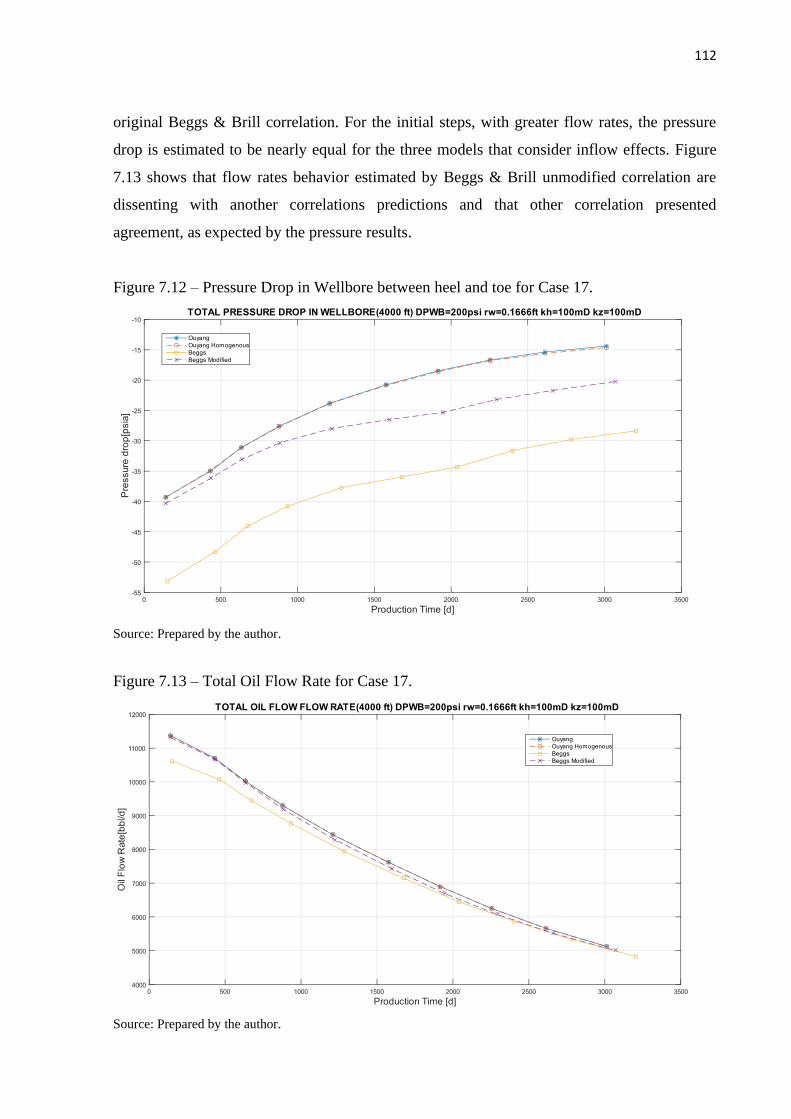
112

original Beggs & Brill correlation. For the initial steps, with greater flow rates, the pressure

drop is estimated to be nearly equal for the three models that consider inflow effects. Figure

7.13 shows that flow rates behavior estimated by Beggs & Brill unmodified correlation are

dissenting with another correlations predictions and that other correlation presented

agreement, as expected by the pressure results.

Figure 7.12 – Pressure Drop in Wellbore between heel and toe for Case 17.


Figure 7.13 – Total Oil Flow Rate for Case 17.


113

Figures 7.14 and 7.15 permit a deeper investigation on the factors behind the small

difference between the modified correlation and Ouyang models. Results for liquid holdup

are in the small range compared to other cases presented. Observing the pressure behavior, the

discontinuities in holdup do not clearly appear.

Figure 7.14 – Liquid holdup in wellbore for the first depletion step - Case 17.


Figure 7.15 – Pressure in wellbore for the first depletion step - Case 17.


114

There is no significant difference on the friction/acceleration losses ratio between the

first step and the last one when the results are not so close; so, the main reason behind that

small gap is the small range of liquid holdup that induces a similar estimate for mixture

properties and consequently a similar estimate for pressure drop. With the increase in the

amount of gas in the wellbore, liquid holdup range raises and the pressure drop estimated by

each correlation eventually differs from the results of other models.

A final observation can be made comparing all the total pressure drops after a

depletion step; this comparison is presented in figure 7.14. Using Ouyang Mechanistic Model

as comparation basis, it is possible to notice that for low pressure drops (generally associated

with low flow rates) the original Beggs & Brill Model estimates smaller losses than the

mechanistic model. However, when the flow rate increases, that relation is reverted. Beggs &

Brill Modified Model estimate greater losses for almost every depletion step, but it generally

presents results that do not deviate much from the 25% difference range for the reference

model; conversely, the original Beggs & Brill deviate significantly, more than 25% for losses

above 5 psi. The homogenous model is consistent with the original Ouyang model.

Figure 7.14 – Total Pressure Drop estimated for each depletion step in every simulation case.


115

8 VERTICAL WELL SIMULATIONS

This chapter is divided into three sections. Firstly, the coupling methods presented in

chapter 6 are compared. Then the influence of well and wellbore correlations in production

prediction is addressed and at last the coupling method is utilized to investigate the impact of

well radius in production. In order to obtain these results, the general characteristics of the

system are presented in Appendix C. Some complementary information is presented here:

- The well length is a variable that is changed according to the simulation; it refers

to the distance between the wellhead and the top of the reservoir formation.

- The well and reservoir radius are variables that are changed according to the

simulation;

- The production zone is also a variable; it is always defined in Zone 1 of the

reservoir structure as presented in Appendix C;

- The well characteristics are presented in Table B.3;

- The Δ𝑡 scheme for coupling simulations is as follows:

Δ𝑡 =

{

1000 𝑠, 𝑖𝑓 𝑇𝑆 < 1001 𝑑, 𝑖𝑓 100 ≤ 𝑇𝑆 < 2002 𝑑, 𝑖𝑓 200 ≤ 𝑇𝑆 < 3003 𝑑, 𝑖𝑓 300 ≤ 𝑇𝑆 < 4004 𝑑, 𝑖𝑓 400 ≤ 𝑇𝑆 < 5005 𝑑, 𝑖𝑓 500 ≤ 𝑇𝑆 < 70010 𝑑, 𝑖𝑓 700 ≤ 𝑇𝑆 < 80020 𝑑, 𝑖𝑓 800 ≤ 𝑇𝑆

(8.1)

- The top-hole pressure behavior that is controlled by the algorithm :

• The pressure is calculated by equation 8.2 until it falls below 780 𝑝𝑠𝑖; then 780

𝑝𝑠𝑖 is assumed. This is adapted from Schietz (2009) start-up method.

𝑇𝐻𝑃(𝑝𝑠𝑖) = (−0.85979 𝑡𝑚𝑖𝑛

(1 + 𝑒−0.03984(𝑡𝑚𝑖𝑛−120.53))) + 887.52 (8.2)

• After that start-up process, if the oil flow rate for a time step is lower than 1000

𝑏𝑏𝑙/𝑑, 𝑇𝐻𝑃 is reduced by 50 𝑝𝑠𝑖 until it reaches 580 𝑝𝑠𝑖, which is the

minimum wellhead pressure considered.

With this information it is possible to reproduce any result presented in this chapter.

116

8.1 COUPLING METHODS

The 4 coupling methods were tested in 8 simulation cases; for these simulations, the

tolerance considered is 10−3, 𝑟𝑤 = 0.1458 𝑓𝑡, 𝑟𝑒 = 1500 𝑓𝑡 and the length of production

zone is 20 𝑓𝑡. The results are presented in three complementary ways. Table 8.1 shows the

reason why a simulation ends, the ideal result for this is “No operation point reached”; this

implies that the simulation works but physically it is impossible to sustain production using

reservoir natural energy. The second way to present the results is to show a brief description

on how the simulation ends. Finally, the number of iterations required by each coupling are

compared.

Table 8.1- Coupling methods results for 8 simulation cases. Well

Length (m) COUP1 COUP2 COUP3 COUP4

H&B 1500 Numerical Failure (1,1)

UNCLEAR (1,2)

UNCLEAR (1,3)

Numerical Failure (1,4)

H&B 2000 Numerical Failure (2,1)

UNCLEAR (2,2)

UNCLEAR (2,3)


B&H 1500 No operation point reached

(3,1)

No operation point reached

(3,2)


(3,3)


(3,4)

B&H 2000 No operation point reached

(4,1)


(4,2)


(4,3)


(4,4)

C&L 1500 No operation point reached

(5,1)




(5,4)

C&L 2000 No operation point reached

(6,1)




(6,4)

B&B 1500 No operation point reached

(7,1)


(7,2)


(7,3)


(7,4)

B&B 2000 Production did not start

(8,1)

Production did not start

(8,2)


(8,3)


(8,4)

Source: Prepared by the author,2020.

Table 8.1 shows that COUP1 and COUP4, both methods based on two iterations

loops, presented the same final causes for simulation endings; these causes are different than

the ones for COUP2 and COUP3, methods with only one loop. Although at first glance the

two-loop methods are more secure, since they simulate 5 of 7 cases until the end of the

117

reservoir productive life, the failures presented by methods 2 and 3 are a consequence of very

low flow rates (a characteristic of Chexall & Lellouche correlation). The description of how

each simulation ends (the simulations are identified by their position in Table 8.1) helps to

clarify the information encountered.

Simulation (1,1) - The coupling method fails to advance to time step 1013 and it also

fails to reduce wellbore residue. It probably occurs because solution to wellbore pressures

oscillates between two vectors. BHP was stable for time step 1012 and total oil flow rate

swings between 612.732 and 612.736 bbl/d.

Simulation (1,2) - The coupling method fails to advance to time step 2067; the

numerical method to guess BHP was frequently inducing great production and consequently

causing a numerical error in the well results; when the guess value is robust, the producing

point was not found, so it is unclear if it is a numerical failure or the end of production.

Simulation (1,3) - The coupling method fails to advance to time step 2069; the failure

can be described as in Simulation (1,2).

Simulation (1,4) - The coupling method fails to advance to time step 1449; the failure

can be described as in Simulation (1,1), except that for this case oil flow rate swings between

508.063 and 508.071 bbl/d.

Figure 8.1 presents the necessary number of iterations (reservoir iteration) to advance

a time step in each coupling method; in the first step (0) COUP1 and COUP4 take more

iterations to reach the operation point than one- loop methods, but after that they generally

keep their iterations below 10. It is possible to observe that when COUP4 closes to time step

of failure, the number of iterations increases significantly which is an indication of a change

in reservoir behavior.

Figure 8.2 presents the oil flow behavior for Case 1; all the coupling methods present

little difference among the results obtained, except by the end of production. It is possible to

observe that COUP4 fails when the oil flow rate curve changes its inclination. The reason

behind this change will be addressed in the next section. This oil flow rate curves generally

shows this kind of results in this coupling comparison, so, except in special cases, they will

not be presented.

118

Figure 8.1- Iterations of coupling methods for Case 1 every 50 time steps.


Figure 8.2- Oil Flow Rate for Case 1.


Simulation (2,1)-The coupling method fails to advance to time step 227; the failure

apparently occurs because the method is incapable of reducing wellbore flow rates errors

which can be a consequence of iterate well and reservoir and after that include wellbore

simulation.

119





Simulation (2,4)-The coupling method fails to advance to time step 4493. Although it

is possible to produce more, according to results using other methods, there is no indication of

numerical failure that makes convergence impossible. The BHP value obtained can satisfy the

tolerance; therefore, a value in wellbore was considered intolerable.

In Figure 8.3 it is possible to observe that COUP4 shows a similar pattern to the one

presented in Case 1, which means that the start-up requires more than 100 iterations and after

that the number of iterations remains low. COUP1 struggles to obtain a solution for time step

200 and then fails in time step 227. COUP2 and COUP3, in general, need significantly more

iterations than coupling 1 to advance a time step; these correlations obtain very similar results.



Simulation (3,1)-The coupling method fails to advance to time step 494; it fails to find

a viable BHP too.


a viable BHP too.

120


a viable BHP too.


a viable BHP too.

Figure 8.4 shows the number of iterations that are utilized by each coupling method in

Case 3; COUP2 and COUP3 presented again a similar behavior, needing more reservoir

simulations to obtain the operation point than COUP1 and COUP4, except for the first time

step.




a viable BHP too.


a viable BHP too.


a viable BHP too.


a viable BHP too.

Figure 8.5 presents almost the same pattern shown in figure 8.4, except that for Case

5, the two-loop couplings presented a raise in the number of iterations after time step 300. An

121

important fact about this simulation is that the computational time for well simulation was

longer using Barbosa & Hewitt correlation than using other correlations that do not consider

the flow pattern in its calculations; this implies an advantage for COUP4 since this method

does not require well calculations for all iterations.



Simulation (5,1) - The coupling method fails to advance to time step 709; it fails to

find a viable BHP too.

Simulation (5,2) - The coupling method fails to advance to time step 559; it fails as

guess value for BHP induces a high flow rate from reservoir.

Simulation (5,3) - The coupling method fails to advance to time step 581; it is unclear

why it failed, but it is probable that it induces injection flow rate after 844 iterations.

Simulation (5,4) - The coupling method fails to advance to time step 707; it fails to

find a viable BHP too.

Figure 8.6 indicates an increase in the number of iterations when the reservoir energy

is reduced. For this case, relevant information about failures can be obtained observing the oil

flow rates results near the time when coupling methods 2 and 3 failed. In figure 8.7 it is

possible to observe that production is below 80 𝑏𝑏𝑙/𝑑 and that the results for each method

oscillate around a tendency. The two-loop method presented more consistency on this

122

oscillation; it starts with intervals in which the inclination almost remains constant, then its

inclination changes for a time step and returns to the original value. One-loop method does

not present a pattern in that oscillation; so it is possible that this random behavior, combined

with low flow rates, induced these methods to fail.



Figure 8.7- Oil Flow Rate for Case 5.


123


a viable BHP too.

Simulation (6,2)-The coupling method fails to advance to time step 598; it is probable

that the method induces injection flow rate after 539 iterations.

Simulation (6,3)-The coupling method fails to advance to time step 596; the numerical

error was unclear. Some negative oil flow rates are obtained during the iterations.


a viable BHP too.

Figure 8.8 shows a difference in the pattern of COUP1 and COUP4 results. In Case 6,

their iterations do not increase probably as a consequence of the reservoir energy that is

greater than in Case 5. A relevant observation about Chexall & Lellouche simulations is that

two loops methods found operation points even for 3 𝑏𝑏𝑙/𝑑 oil flow rate, which is almost

certainly an unrealistic result. So, the fact that they simulated these scenarios are not an

advantage in relation to COUP2 and COUP3.



Simulation (7,1)-The coupling method faild to advance to time step 382; it fails to find

a viable BHP too.

124


a viable BHP too.


a viable BHP too.


a viable BHP too.

Just as in Case 3, all simulations for Case 7 ended in the same time step. Case 7 also

presented, after step 100, two perfect matches. COUP1 and COUP4 as well as COUP2 and

COUP3 showed the same number of iterations in each time step.



Simulation (8,1)-The coupling method fails to find an operation point for reservoir

start-up.

Simulation (8,2)- The coupling method fails to find an operation point for reservoir

start-up.


start-up.


start-up.

125

In Case 8, there is no production, and thus, no iteration graphic. The combination of

all observations results is some conclusions:

- COUP1 and COUP4 presented similar results.

- COUP2 and COUP3 presented similar results.

- One-loop coupling requires more iterations than two-loop coupling.

- One-loop coupling performs better to the start-up and is more probable to advance

a time step than two-loop coupling.

- One-loop coupling requires an improvement

In the next sections, simulations were performed using COUP3 since there is more

security in one-loop coupling. No significant difference between coupling 2 and coupling 3

was found; COUP3 was chosen for the next simulation only because the simulation order of

the systems seems more natural.

8.2 CORRELATIONS

The impacts of the four correlations for well and the 2 correlations for wellbore were

tested in 8 simulation cases. The tolerance considered for these simulations was 10−2, 𝑟𝑤 =

0.1458 𝑓𝑡 and 𝑟𝑒 = 1500 𝑓𝑡. Tables 8.2 and 8.3 show the number for each simulation

performed.

Table 8.2 – Simulations using Ouyang Homogeneous Wellbore Correlation.

PRODUCTION

ZONE (𝒇𝒕)

WELL

LENGTH (𝒎)

H&B B&H C&L B&B

20 1500 1 2 3 4

20 2000 5 6 7 8

40 1500 9 10 11 12

40 2000 13 14 15 16

60 1500 17 18 19 20

60 2000 21 22 23 24

80 1500 25 26 27 28

80 2000 29 30 31 32


126

Table 8.3 – Simulations using Beggs & Brill Modified Wellbore Correlation.

PRODUCTION

ZONE (𝒇𝒕)

WELL

LENGTH (𝒎)

H&B B&H C&L B&B

20 1500 33 34 35 36

20 2000 37 38 39 40

40 1500 41 42 43 44

40 2000 45 46 47 48

60 1500 49 50 51 52

60 2000 53 54 55 56

80 1500 57 58 59 60

80 2000 61 62 63 64


8.2.1 IMPACT OF WELL CORRELATIONS

In order to estimate the impact of well simulation on reservoir production, only the

simulation results in Table 8.2 will be considered. Figure 8.10 presents the results for oil flow

rate in simulations 1 to 4; the results indicate that Hagedorn & Brown correlation estimates a

production time considerably longer than other correlations. Chexal & Lellouche and Barbosa

& Hewitt Models presented very similar results for production because along most of the

well, the flow pattern found by the Barbosa & Hewitt Model is bubble. For this pattern, the

pressure drop is calculated based on the correlation of Chexal & Lellouche.

Beggs & Brill forecast an initial flow rate above Chexal & Lellouche and Barbosa &

Hewitt Models, but this correlation indicates that reservoir energy sustains production for a

shorter time. A consequence of these two facts, that is not easily noticed in figure 8.11, is that

those three models presented almost the same results for total production. As expected for

figure 8.10, the total production estimated by Hagedorn & Brown is more than 10 times

greater than the production estimated by other correlations.

127

Figure 8.10 – Oil Flow Rate for simulations 1 to 4.


Figure 8.11 – Cumulative oil production for simulations 1 to 4.


128

The BHP behavior presented in figure 8.12 shows that after start-up, every correlation

remains at a quasi-constant value, but the timing of this stability is very different for the

Hagedorn & Brown correlation. It is a 10-day phenomenon in this case and in other situations

this condition remains unaltered until a change in 𝑇𝐻𝑃 occurs. After that period, Hagerdorn &

Brown reduces the pressure demand in the well and this extends the production time.

Though initially Barbosa & Hewitt and Chexal & Lellouche present almost the same

results, for the final days of production the mechanistic model shows a slow growth and

category 2 correlation spikes; this instantenous growth reduces production but permits more

days of production.

Figure 8.12 – BHP for simulations 1 to 4.


Figure 8.13 presents the gas-oil ratio for each model; except for Hagedorn & Brown,

the results found are essentially constant. GOR drops for Hagedorn & Brown correlation

before other simulations end. This drop implies the release of a quantity of gas from oil

located in the reservoir, but its low saturation makes the gas phase immobile in the reservoir.

Although the total volume of gas produced is reduced, the gas is free at the wellbore and this

implies a reduction in total energy required in well and wellbore.

129

Figure 8.13 – GOR for simulations 1 to 4.


For these four simulations, a complete analysis was made. As results are similar in

other cases, for the aforementioned four simulations only results that bring up new

information are shown. Figures 8.14 and 8.15 show an interesting point: Barbosa & Hewitt

correlation does not present similarities with Chexal & Lellouche correlation in the initial

steps which indicates that bubble flow is not dominant for these steps. After 100 days this

situation changes, and results are almost the same for both correlations.

Another observation that should be made is that even when the initial production

estimated by Hagedorn & Brown correlation is smaller compared to other correlations, the

estimated production time is longer. Figure 8.15 shows that the phenomenon of the drop in

BHP after a stability period is a consequence of correlation itself and not an effect of reservoir

transmitted to the well. This makes the pressure estimated by Hagedorn & Brown to fall

below the pressures values estimated by other correlations and bubble point (2000 psi)

allowing free gas flow throughout the wellbore.

130



Figure 8.15 – BHP for simulations 25 to 28.


Figure 8.16 shows the production predicted by simulations 21 to 24; an interesting

observation about this figure is that Beggs & Brill predicts more production than Barbosa &

Hewitt and Chexal & Lellouche. This is an important observation because for simulation 8,

131

category 3 correlation does not find a operation point to start-up. In fact, the behavior of

Beggs & Brill is the most sensitive to variations in the length of the production zone.



Other results do not bring up any new information. In a single sentence, the conclusion

of this section is that well correlation influences coupling production results a lot. So, in order

to simulate a field, it is important to consider which correlation best fit the well test results.

8.2.2 WELLBORE CORRELATIONS IMPACT

Ouyang Homogeneous Model and Beggs and Brill Modified Model were utilized for

simulation purposes. Each simulation that applied the homogeneous model in Table 8.2 has a

counterpart that used the modified model in Table 8.3. The results for oil flow rate obtained

by simulations 29 and 61 are presented in figure 8.17.

132

Figure 8.17 – Oil Flow Rate for simulations 29 and 61.


The results demonstrate that the wellbore method does not impact too much on the

production results, although Beggs & Brill Modified Model predicts a longer production time,

the time difference does not imply a significant difference in total production (around 5%).

The total pressure drop in wellbore remais at around 26 psi during production for both

correlations; in fact, the results for wellbore in the first time step are exactly the same. As a

consequence of these observation it is possible to suggest that the difference in production

time is a consequence of random guessing combined with COUP 3 failures for small flow

rates.

The comparison of results obtained by simulations 20 and 52 are shown in figure 8.18;

these results confirm the small impact of wellbore simulation in coupling results (the sum of

losses in wellbore was around 19 psi during production time). In fact, all 32 comparisons of

Table 8.2 and Table 8.3 presented this pattern; as a consequence, showing other results is

redundant. The main conclusion of this section is that unless the production zone represents a

significant portion of the well, the model utilized for its simulation is irrelevant for production

results.

133

Figure 8.18 – BHP for simulations 20 and 52.


8.3 WELL RADIUS

This section is intended to show how coupling simulations could be important to

define production strategies. Although the program developed is very simple and limited

when compared with a commercial software, it is possible to perform simulations to

understand how a variable impacts on the system. In order to exemplify that, the results

obtained with two well radii are compared in 9 simulations cases as presented in Table 8.4.

The tolerance considered for these simulations is 10−2, the length of production zone is 20 𝑓𝑡

and the well length is 2000 𝑚.

Table 8.4 shows the results for total production with two values for 𝑟𝑤 and the

percentual decrement when producing with larger radius. Hagedorn & Brown simulations

estimate greater values for total production than other correlations which results in

consistency among the results obtained for production decrement using a larger well. In fact,

for Hagerdorn & Brown, the initial oil flow rate is smaller when producing with smaller

radius, but production time is longer, and it induces an increment in total production as

presented in figure 8.20.

134

Table 8.4 – Production results with two well radii

𝑟𝑒 (𝑓𝑡) Well

Correlation

Total Production (𝑏𝑏𝑙)

𝑟𝑤 = 0.1463 𝑓𝑡

Total Production (𝑏𝑏𝑙)

𝑟𝑤 = 0.1875 𝑓𝑡

%

Production

Variation

1500 B&H 327861 292913 -10.66

2000 B&H 652018 531713 -18.45

2500 B&H 1007748 897134 -10.98

1500 C&L 347119 358236 -3.10

2000 C&L 594633 679762 -12.52

2500 C&L 885518 920818 -3.83

1500 H&B 18948085 20744665 -8.66

2000 H&B 34876996 37532274 -7.08

2500 H&B 55891138 59891747 -6.68


For Barbosa & Hewitt and Chexall & Lellouche, the initial oil flow rate is greater

when producing with smaller radius; this occurs due to a deeper release of gas into the well

that reduces 𝐵𝐻𝑃. Still on these correlations, the decrement in production for cases with 𝑟𝑒 =

2000 𝑓𝑡 is considerably bigger than in other simulations; this occurs because with smaller

well radius, the coupling method found an operation point with a greater value for 𝐵𝐻𝑃 when

the results of oil flow rate are closer to the value of reservoir death using 𝑟𝑤 = 0.1875 𝑓𝑡.

It is clear in Table 8.4 that there is a decrement in total production using a larger

diameter. The percentual value of this decrease could be very decisive in production

situations; a smaller diameter could imply more investment in drilling and completion.

Probably a 3.10% increase(line four in the table 8.4) in barrels produced will not provide a

return on the initial capital invested.

Figure 8.19 and 8.20 demonstrate that the well radius shifts production results. In

some cases, BHP is reduced when 𝑟𝑤 decreases and as consequence, the oil flow rate

increases. On the other hand, when producing at low flow rates, the reservoir energy is

preserved and it has more time to be restored by gravitational effects; production time is

longer so it is possible that for some situations a thinner well will increase total production

even when it gets started with a low flow rate.

135

Figure 8.19– BHP for simulations of line 5 of Table 8.4.


Figure 8.20 – Oil Flow Rate for simulations of line 9 of Table 8.4.


136

9 CONCLUSIONS

The main objective of this work was to develop a well-reservoir coupling method for

vertical simulations using a transient reservoir simulator and a steady-state well simulator.

During the development of this work, horizontal well results were needed and so, a simplified

reservoir simulator was developed to proceed with the simulations. Both methods were

successfully programmed and obtained reasonable results.

The proposed well simulator was broken in two simulators during this work; each one

using a specific approach. The first one, targeted at the region of well that do not receive

influx from reservoir, maintained the name “well”. The program for this region was

developed by Alves, E.(2017) and originally coupled with reservoir by Alves, R. (2017). The

second region is the one under reservoir inflow, namely “wellbore”; the related simulator was

fully developed exclusively for this work using as reference the work of Ouyang (1998).

The horizontal well simulations were performed in order to measure the impact of

adapting the correlation developed by Beggs and Brill (1983) to consider radial influx; this

correlation was compared with the modified model developed by this work and with the

mechanistic and homogenous models presented by Ouyang (1998) as both were developed

using radial influx as reference experiments. The results showed that, in general, Modified

Beggs & Brill correlation pressure drop calculation was more consonant with Ouyang (1998)

models than with the original correlation, although liquid holdup results were very similar

with or without modification.

As the well model was broken in two simulators, 4 methods were developed to couple

the reservoir with these two simulators; the differences between these methods were the

simulation order and the way they were iterated - either using one or two loops. The four

coupling methods were utilized to simulate eight production cases and the results of these

simulations permitted two main observations:

- The methods that utilize two loops (COUP1 and COUP4) needed fewer iterations to

advance a time step.

- The methods that utilize one loop (COUP2 and COUP3) are less susceptible to

numerical errors.

The well program permits to utilize the correlations developed by Hagedorn and

Brown (1965), Beggs and Brill (1973), Chexal et al. (1992) and Barbosa and Hewitt (2006)

and the wellbore program permits to utilize the Modified Beggs & Brill correlation and the

137

homogeneous Ouyang (1998) model. Thus, in order to evaluate the impact of correlations in

production, 8 systems were simulated using the 8 combinations of well and wellbore

correlations to obtain 64 simulations. These 64 simulations were compared, and the outcome

showed that:

- Well simulator correlations are very important to the production results; the coupling

results could even change the scale of oil produced according to the correlation

utilized.

- Altought for initial time steps each well correlation predicts a different flow rate, the

main difference in total production results is a consequence of gas liberation in

reservoir.

- Chexal & Lellouche and Barbosa & Hewitt correlations presented very similar results

in most correlations; this observation indicates a dominance of bubble flow in the

well.

- Wellbore results indicate that the correlation utilized for this region was not impactful

in the results; this is a consequence of the production zone length and of the small

presence of gas in this region.

Finally, the coupling simulator was utilized to compare two well radii in 9

configurations. The results of these simulations showed that a smaller radius induces a greater

production. The reasons behind this increase in production changes according to the

correlation utilized to simulate the well; for Hagedorn & Brown, a smaller initial flow rate

sustains the production for a long time; for the other correlations, the reservoir has a short life

but the initial flow rate is lower for larger diameters.

As such, the primary and secondary objectives of this work were fulfilled. Regarding

recommendations for future studies, a few topics of interest were identified:

- An investigation about the possibility of adapting two-phase flow models to consider

lateral influx.

- To develop a combination of the two and one-loop methods, utilizing two-loop

methods to reduce iterations and one-loop methods to increase the probability of

convergence.

- To test a coupling method with unified well and wellbore models using only the

pressures and flows at the wellbore as variables to be tested during iterations; this will

reduce the necessity of data exchange between well and wellbore models.

138

- To implement and compare more multiphase flow models and to run tests with more

reservoir models, preferably real field data, in order to better understand how

impactful these models are in a variety of situations.

- To develop a program that utilizes real field data to check which well model best

matches these data.

- To improve the program to perform a better representation of real fields, including gas

lift in the well, injection in reservoir, aquifer representation, gas in water solution and

so on.

- To perform simulations to investigate the liquid load formation in the well and

formation of a U-curve for the pressure in the reservoir; in order to do that it will be

necessary to allow for negative velocities in the well.

139

REFERENCES

ABOU-KASSEM, Jamal; ALI, S. Farouq; ISLAM, M. Rafiq. Petroleum Reservoir

Simulations. Houston: Gulf Publishing Company, 2006.

ALBERTS, Garrelt et al. An Investigation Into the Need of a Dynamic Coupled Well-

Reservoir Simulator. SPE Annual Technical Conference And Exhibition, [s.l.], p.1-9,

2007. Society of Petroleum Engineers. http://dx.doi.org/10.2118/110316-ms.

ALMEHAIDEB, R.A.; AZIZ, K.; PEDROSA, O.A.. A Reservoir/Wellbore Model for

Multiphase Injection and Pressure Transient Analysis. Middle East Oil Show, [s.l.], p.1-10,

1989. Society of Petroleum Engineers. http://dx.doi.org/10.2118/17941-ms.

ALVES, Eduardo Bader Dalfovo Mohr; ALVES, Marcus Vinicius Canhoto; ALVES, Rafael

Joaquim. Comparison of two phase flow correlation predictions with the black oil model. In:

RIO PIPELINE, 11., 2017, Rio de Janeiro. Rio de Janeiro: IBP, 2017. p. 1 - 9.

ALVES, Eduardo Bader Dalfovo Mohr. COMPARAÇÃO DE CORRELAÇÕES

BIFÁSICAS EM CONDIÇÕES DE POÇOS PRODUTORES. 2017. 106 f. TCC

(Graduação) - Curso de Engenharia de Petróleo, Engenharia de Petróleo, UDESC, Balneário

Camboriú, 2017. <http://sistemabu.udesc.br/pergamumweb/vinculos/000041/000041dc.pdf>.

ALVES, Rafael Joaquim. UM MODELO DE ACOPLAMENTO POÇO

RESERVATÓRIO. 2017. 113 f. TCC (Graduação) - Curso de Engenharia de Petróleo,

Engenharia de Petróleo, Udesc, Balneário Camboriú, 2017. Disponível em:

<http://sistemabu.udesc.br/pergamumweb/vinculos/000044/0000443d.pdf>. Acesso em: 10

jan. 2020.

ASHEIM, Harald; KOLNES, Johnny; OUDEMAN, Piet. A flow resistance correlation for

completed wellbore. Journal Of Petroleum Science And Engineering, [s.l.], v. 8, n. 2, p.97-

104, set. 1992. Elsevier BV.

AZADI, Mohsen; AMINOSSADATI, Saiied Mostafa; CHEN, Zhongwei. Numerical

Simulation of Integrated Reservoir Borehole Flow for Pre-Mining Drainage. In: COAL

OPERATORS' CONFERENCE, 16., 2016, Wollongong. Proceedings of the 16th Coal

Operators' Conference. Wollongong: Uow, 2016. p. 249 – 262

BARBOSA, J. and HEWITT, G., 2006. “Gas-liquid two-phase flow in vertical pipes-a

description of models used in the gramp2 programme”. Technical report, Internal Report,

Imperial College.

http://dx.doi.org/10.2118/110316-ms


140

BARNEA, Dvora. Transition from annular flow and from dispersed bubble flow—unified

models for the whole range of pipe inclinations. International Journal of Multiphase Flow,

[S.l.], v. 12, n. 5, p.733-744, set. 1986. Elsevier BV. http://dx.doi.org/10.1016/0301-

9322(86)90048-0.

BARNEA, Dvora; BRAUNER, Neima. Holdup of the liquid slug in two phase intermittent

flow. International Journal of Multiphase Flow, [S.l.], v. 11, n. 1, p.43-49, jan. 1985.

Elsevier BV. http://dx.doi.org/10.1016/0301-9322(85)90004-7.

BARNEA, Dvora; SHOHAM, Ovadia; TAITEL, Yehuda. Flow pattern transition for

downward inclined two phase flow; horizontal to vertical. Chemical Engineering Science,

[S.l.], v. 37, n. 5, p.735-740, 1982. Elsevier BV. http://dx.doi.org/10.1016/0009-

2509(82)85033-1.

BARNEA, Dvora; SHOHAM, Ovadia; TAITEL, Yehuda. Flow pattern transition for vertical

downward two phase flow. Chemical Engineering Science, [S.l.], v. 37, n. 5, p.741-744,

1982. Elsevier BV. http://dx.doi.org/10.1016/0009-2509(82)85034-3.

BEGGS, D.H.; BRILL, J.P.. A Study of Two-Phase Flow in Inclined Pipes. Journal Of

Petroleum Technology, [S.l.], v. 25, n. 05, p.607-617, 1 may 1973. Society of Petroleum

Engineers (SPE). http://dx.doi.org/10.2118/4007-pa.

BEGGS, H. Dale. Production System Analysis. In: BEGGS, H. Dale. Production

Optimization: Using NODAL Analysis. Tulsa: Ogci, 1994. Cap. 1, p. 1.

BP ENERGY ECONOMICS. BP Energy Outlook 2019 Edition. Londres: BP, 2019. 137 p.

BRET-ROUZAUT, Nadine; FAVENNEC, Jean-pierre. Investments and costs. In: BRET-

ROUZAUT, Nadine; FAVENNEC, Jean-pierre. Oil and Gas Exploration and Production:

Reserves, costs, contracts. 3. ed. Paris: Technip, 2011. Cap. 4. p. 121-167.

BYRNE, Michael T. et al. Computational Fluid Dynamics for Reservoir and Well Fluid Flow

Performance Modelling. Spe European Formation Damage Conference, [s.l.], p.1-7, 2011.

Society of Petroleum Engineers. http://dx.doi.org/10.2118/144130-ms.

CHEN, Zhangxin; HUAN, Guanren; MA, Yuanle. Computational Methods for Multiphase

Flows in Porous Media. Dallas, Texas: SIAM, 2006.

CHEXAL, B. et al. A void fraction correlation for generalized applications. Progress In

Nuclear Energy, [s.l.], v. 27, n. 4, p.255-295, jan. 1992. Elsevier BV.

http://dx.doi.org/10.1016/0149-1970(92)90007-p.

http://dx.doi.org/10.1016/0301-9322(86)90048-0

http://dx.doi.org/10.1016/0301-9322(86)90048-0

http://dx.doi.org/10.1016/0301-9322(85)90004-7

http://dx.doi.org/10.1016/0009-2509(82)85033-1

http://dx.doi.org/10.1016/0009-2509(82)85033-1

http://dx.doi.org/10.1016/0009-2509(82)85034-3

http://dx.doi.org/10.2118/4007-pa


http://dx.doi.org/10.1016/0149-1970(92)90007-p

141

CHEXAL, Bindi; LELLOUCHE, Gerald. Full-range drift-flux correlation for vertical

flows. Revision 1. Palo Alto: Inis, 1986.

CHUPIN, Gael et al. Integrated Wellbore/Reservoir Model Predicts Flow Transients in

Liquid-Loaded Gas Wells. Spe Annual Technical Conference and Exhibition, [S.l.], p.1-

11, 2007. Society of Petroleum Engineers. http://dx.doi.org/10.2118/110461-ms.

CLEGG, John (Ed.). Petroleum Engineering Handbook: Production Operations

Engineering. Richardson: SPE, 2007.

CONINCK, Arne de et al. Needles: Toward Large-Scale Genomic Prediction with Marker-by-

Environment Interaction. Genetics, [S.l.], v. 203, n. 1, p.543-555, 2 mar. 2016. Genetics

Society of America. http://dx.doi.org/10.1534/genetics.115.179887.

DEMPSEY, J.r. et al. An Efficient Model for Evaluating Gas Field Gathering System Design.

Journal Of Petroleum Technology, [s.l.], v. 23, n. 09, p.1067-1073, 1 set. 1971. Society of

Petroleum Engineers (SPE). http://dx.doi.org/10.2118/3161-pa.

DICKSTEIN, F. et al. Modeling and Simulation of Horizontal Wellbore-Reservoir Flow

Equations. Latin American And Caribbean Petroleum Engineering Conference, [s.l.],

p.1-8, 1997. Society of Petroleum Engineers. http://dx.doi.org/10.2118/39064-ms.

DUMKWU, Francis A.; ISLAM, Akand W.; CARLSON, Eric S.. Review of well models and

assessment of their impacts on numerical reservoir simulation performance. Journal Of

Petroleum Science And Engineering, [s.l.], v. 82-83, p.174-186, fev. 2012. Elsevier BV.

http://dx.doi.org/10.1016/j.petrol.2011.12.005.

ECONOMIDES, Michael et al. Petroleum Production Systems. 2. ed. New Jersey: Prentice

Hall, 2013.

EGBE, Thankgod; SANNI, Gideon; CHIROMA, Abba. Advances in WRFM Technology

Integration. Spe Nigeria Annual International Conference And Exhibition, [s.l.], p.1-9,

2018. Society of Petroleum Engineers. http://dx.doi.org/10.2118/193528-ms

EQUAÇÕES Diferenciais Ordinárias: Problemas de Valor Inicial. In: GILAT, Amos;

SUBRAMANIAM, Vish. Métodos Numéricos para Engenheiros e Cientistas: Uma


http://dx.doi.org/10.1534/genetics.115.179887

https://eur05.safelinks.protection.outlook.com/?url=http%3A%2F%2Fdx.doi.org%2F10.2118%2F3161-pa&data=02%7C01%7C%7C2284e3300ead46e5af0608d7beeafc15%7C84df9e7fe9f640afb435aaaaaaaaaaaa%7C1%7C0%7C637187788763847093&sdata=1n%2FcradT2WmBYke97PwteUsjzdMxy%2F%2Bch0lRAM%2FT4sc%3D&reserved=0


http://dx.doi.org/10.1016/j.petrol.2011.12.005


142

introdução com aplicações usando o MATLAB. Porto Alegre: Bookman, 2008. Cap. 8. p.

327-347.

ERTEKIN, Turgay; ABOU-KASSEM, Jamal; KING, Gregory. Basic Applied Reservoir

Simulation. Richardson, Texas: SPE, 2001.

FEKETE. Wellbore Configuration. Disponível em:

<http://www.fekete.com/SAN/TheoryAndEquations/VirtuWellTheoryEquations/c-sw-

wellbore.htm>. Acesso em: 10 fev. 2020.

FIROOZABADI, H. M. et al. Analysis of Production Logging Data to Develop a Model to

Predict Pressure Drop in Perforated Gas Condensate Wells. Petroleum Science And

Technology, [s.l.], v. 29, n. 16, p.1722-1732, 8 jul. 2011. Informa UK Limited.

http://dx.doi.org/10.1080/10916461003620420

FOX, Robert; MCDONALD, Alan; PRITCHARD, Philip. Escoamento Interno Viscoso e

Incompressível. In: FOX, Robert; MCDONALD, Alan; PRITCHARD, Philip. Introdução a

Mecânica dos Fluidos. 8. ed. Rio de Janeiro: LTC, 2014.

FRIEDEL, L. Improved friction pressure drop correlations for horizontal and vertical two-

phase pipe flow. In: European two-phase group meeting, Ispra, Italy. [S.l.: s.n.], 1979.

GOVIER, G. W.; AZIZ, Khalid. The flow of complex mixtures in pipes. New York: Van

Nostrand Reinhold Company, 1972. 792 p.

GUO, B.; LYONS, W. C.; GHALAMBIR, A. Petroleum Production Engineering, A

Computer-Assisted Approach. Elsevier Science, 2007. ISBN 0750682701. Disponível

em:<https://books.google.com.br/books?id=LKn-oVIHXDUC>.

HAGEDORN, Alton R.; BROWN, Kermit E.. Experimental Study of Pressure Gradients

Occurring During Continuous Two-Phase Flow in Small-Diameter Vertical Conduits.

Journal Of Petroleum Technology, [s.l.], v. 17, n. 04, p.475-484, 1 abr. 1965. Society of


HINZE, J. O.. Fundamentals of the hydrodynamic mechanism of splitting in dispersion

processes. Aiche Journal, [s.l.], v. 1, n. 3, p.289-295, set. 1955. Wiley.

http://dx.doi.org/10.1002/aic.690010303.

HOFFMANN, A.; STANKO, Milan; GONZÁLEZ, Diana. Optimized production profile

using a coupled reservoir-network model. Journal Of Petroleum Exploration And

Production Technology, [s.l.], p.1-15, 24 jan. 2019. Springer Nature.

http://dx.doi.org/10.1007/s13202-019-0613-1.

https://eur05.safelinks.protection.outlook.com/?url=http%3A%2F%2Fdx.doi.org%2F10.1080%2F10916461003620420&data=02%7C01%7C%7C851b442607294f28110108d7a53c0ea0%7C84df9e7fe9f640afb435aaaaaaaaaaaa%7C1%7C0%7C637159549665851619&sdata=AHHb6ZO00keB%2BjeXgbKb0u4it1HwAyrfNbe3%2BUL7sDA%3D&reserved=0


http://dx.doi.org/10.1002/aic.690010303

http://dx.doi.org/10.1007/s13202-019-0613-1

143

HOLMES, J.a.; BARKVE, T.; LUND, O.. Application of a Multisegment Well Model to

Simulate Flow in Advanced Wells. European Petroleum Conference, [s.l.], p.1-15, 1998.

Society of Petroleum Engineers. http://dx.doi.org/10.2118/50646-ms.

INGERSOLL, Christina; LOCKE, Richard M.; REAVIS, Cate. BP and the Deepwater

Horizon Disaster of 2010. 2010. Disponível em:

<https://mitsloan.mit.edu/LearningEdge/operations-management/BP-Deepwater-Horizon-

Disaster/Pages/BP-and-the-Deepwater-Horizon-Disaster-of-2010.aspx>. Acesso em: 04 fev.

2020.

INTERNATIONAL ENERGY AGENCY. World Energy Outlook 2018. Paris: IEA, 2018.

JOHANSEN, Thormod E.; KHORIAKOV, Vitaly. Iterative techniques in modeling of multi-

phase flow in advanced wells and the near well region. Journal Of Petroleum Science And

Engineering, [s.l.], v. 58, n. 1-2, p.49-67, ago. 2007. Elsevier BV.

http://dx.doi.org/10.1016/j.petrol.2006.11.013.

KORDYBAN, E. S.; RANOV, T.. Mechanism of Slug Formation in Horizontal Two-Phase

Flow. Journal Of Basic Engineering, [s.l.], v. 92, n. 4, p.857-865, 1970. ASME

International. http://dx.doi.org/10.1115/1.3425157.

KOUROUNIS, Drosos; FUCHS, Alexander; SCHENK, Olaf. Toward the Next Generation of

Multiperiod Optimal Power Flow Solvers. Ieee Transactions On Power Systems, [s.l.], v.

33, n. 4, p.4005-4014, jul. 2018. Institute of Electrical and Electronics Engineers (IEEE).

http://dx.doi.org/10.1109/tpwrs.2017.2789187.

MALISKA, Clovis. Transferência de Calor e Mecânica dos Fluidos Computacional. 2. ed.

Rio de Janeiro: LTC, 2014.

MÉTODOS abiertos. In: CHAPRA, Steven C.; CANALE, Raymond P.. Métodos numéricos

para ingenieros. 5. ed. México, D. F.: Mcgraw-hill, 2007. p. 154-159.

MILLER, Constance W.. Wellbore Storage Effects in Geothermal Wells. Society of

Petroleum Engineers Journal, [s.l.], v. 20, n. 06, p.555-566, 1 dez. 1980. Society of


NUNES, G. C.; SILVA, A. H. da; ESCH, L. G.. A Cost Reduction Methodology for Offshore

Projects. Offshore Technology Conference, [S.l.], p.1-13, 2018. Offshore Technology

Conference. http://dx.doi.org/10.4043/28898-ms.


http://dx.doi.org/10.1016/j.petrol.2006.11.013

http://dx.doi.org/10.1115/1.3425157

http://dx.doi.org/10.1109/tpwrs.2017.2789187



144

OFFOR, Uchechukwu Herbert; ALABI, Sunday Boladale. An Accurate and Computationally

Efficient Explicit Friction Factor Model. Advances In Chemical Engineering And Science,

[s.l.], v. 06, n. 03, p.237-245, 2016. Scientific Research Publishing, Inc,.

http://dx.doi.org/10.4236/aces.2016.63024.

OUYANG, Liang-Biao. General Single Phase Wellbore Flow Model. Stanford, CA:

Stanford University, 1997.

OUYANG, Liang-biao. Single Phase and Multiphase Fluid Flow in Horizontal Wells.

1998. 268 f. Tese (Doutorado) - Curso de Petroleum Engineering, Stanford University, Palo

Alto, 1998.

OUYANG, Liang-biao; ARBABI, Sepehr; AZIZ, Khalid. General Wellbore Flow Model for

Horizontal, Vertical, and Slanted Well Completions. Spe Journal, [s.l.], v. 3, n. 02, p.124-133,

1 jun. 1998. Society of Petroleum Engineers (SPE). http://dx.doi.org/10.2118/36608-pa.

OUYANG, Liang-biao; AZIZ, Khalid. A MECHANISTIC MODEL FOR GAS–LIQUID

FLOW IN HORIZONTAL WELLS WITH RADIAL INFLUX OR OUTFLUX. Petroleum

Science and Technology, [s.l.], v. 20, n. 1-2, p.191-222, 22 fev. 2002. Informa UK Limited.

http://dx.doi.org/10.1081/lft-120002095.

OUYANG, Liang-biao; AZIZ, Khalid. A Simplified Approach to Couple Wellbore Flow and

Reservoir Inflow for Arbitrary Well Configurations. Spe Annual Technical Conference And

Exhibition, [s.l.], p.1-13, 1998. Society of Petroleum Engineers.

http://dx.doi.org/10.2118/48936-ms.

PARDISO SOLVER PROJECT. PARDISO. Disponível em: <https://pardiso-project.org/>.

Acesso em: 01 fev. 2020.

PERMADI, Pudji. New Formulas for Estimating Productivity of Horizontal Wells. In:

ANNUAL CONVENTION-INDONESIAN PETROLEUM ASSOCIATION, 22., 1993,

Jacarta. Proceedings... . Jacarta: AAPG, 1993. v. 2, p. 131 - 144.

PERMADI, P.. Practical Methods to Forecast Production Performance of Horizontal Wells.

SPE Asia Pacific Oil And Gas Conference, [S.l.], p.1-10, 1995. Society of Petroleum

Engineers. http://dx.doi.org/10.2118/29310-ms.

PETALAS, N.; AZIZ, K. A Mechanistic Model for Stabilized Multiphase Flow in Pipes.

Technical Report for Members of the Reservoir Simulation Industrial Affiliates Program

(SUPRI-B) and Horizontal Well Industrial Affiliates Program (SUPRI-HW), Stanford

University, CA, 1997.

ROOT Finding and Nonlinear Sets of Equation. In: PRESS, William et al. Numerical

Recipes: The Art of Scientific Computing. 3. ed. Cambridge: Cambridge University Press,

2007. Cap. 9. p. 452-454.

http://dx.doi.org/10.4236/aces.2016.63024


http://dx.doi.org/10.1081/lft-120002095



145

ROSA, Adalberto José; CARVALHO, Renato de Souza; XAVIER, José Augusto Daniel.

Engenharia de Reservatórios de Petróleo. Rio de Janeiro: Interciência, 2006.

SAGEN, Jan et al. A Coupled Dynamic Reservoir and Pipeline Model – Development and

Initial Experience. In: INTERNATIONAL CONFERENCE ON MULTIPHASE

PRODUCTION, 13., 2007, Edinburgh. Proceedings [...] . Edinburgh, Uk: Bhr Group, 2007.

p. 1 - 14.

SCHIOZER, Denis José. Simultaneous Simulation of Reservoir and Surface Facilities.

1994. 193 f. Tese (Doutorado) - Curso de Petroleum Engineering, Stanford University, Palo

Alto, 1994.

SCHIETZ, Michael. Optimization of well start-up. 2009. 85 f. Dissertação (Mestrado) -

Curso de Petroleum Production And Processing, Montanuniversität Leoben , Leoben, 2009.

SEGHIDES, T.K. (1984) Estimate Friction Factor Accurately. Chemical Engineering Journal,

91, 63-64

SETTARI, Antonin; AZIZ, Khalid. A Computer Model for Two-Phase Coning Simulation.

Society Of Petroleum Engineers Journal, [s.l.], v. 14, n. 03, p.221-236, 1 jun. 1974. Society

of Petroleum Engineers (SPE). http://dx.doi.org/10.2118/4285-pa.

SETTARI, A.; AZIZ, K.. Use of Irregular Grid in Cylindrical Coordinates. Society Of

Petroleum Engineers Journal, [s.l.], v. 14, n. 04, p.396-412, 1 ago. 1974. Society of

Petroleum Engineers (SPE).

SILVA, D.V. da; JANSEN, J.D.. A Review of Coupled Dynamic Well-Reservoir Simulation,

Delft University of Technology, ENI, Statoil and Petrobras. IFAC, v. 48, n. 6, p.236-241,

2015. Elsevier BV. http://dx.doi.org/10.1016/j.ifacol.2015.08.037.

SIWON, Z., 1987, “Solutions for Lateral Inflow in Perforated Conduits,”

J. Hydraul. Eng., 113(9), pp. 1117-1132.

SOUZA, Grazione de. Acoplamento Poço-Reservatório na Simulação Numérica de

Reservatórios de Gás. 2013. 335 f. Tese (Doutorado) - Curso de Engenharia de Reservatório

e Exploração, Uenf, Macaé, 2013.


http://dx.doi.org/10.1016/j.ifacol.2015.08.037

146

STANDING, M.B. A Pressure-Volume-Temperature Correlation For Mixtures Of California

Oils And Gases. Drilling And Production Practice, Los Angeles, v. 5, n. 45, p.275-287,

May 1947.

STANDING, M. B. Volumetric and Phase Behavior of Oil Field Hydrocarbon Systems.

Dallas: SPE, 1981.

STONE, T.w.; EDMUNDS, N.r.; KRISTOFF, B.j.. A Comprehensive Wellbore/Reservoir

Simulator. SPE Symposium On Reservoir Simulation, p.1-14, 1989. Society of Petroleum


STURM, W.l. et al. Dynamic Reservoir Well Interaction. Spe Annual Technical Conference

And Exhibition, p.1-13, 2004. Society of Petroleum Engineers.


SU, Ze; GUDMUNDSSON, J.S.. Friction Factor of Perforation Roughness in Pipes. SPE

Annual Technical Conference And Exhibition, [S.l.], p.1-13, 1993. Society of Petroleum


TAITEL, Yehuda; BARNEA, Dvora; DUKLER, A. E.. Modelling flow pattern transitions for

steady upward gas-liquid flow in vertical tubes. Aiche Journal, [S.l.], v. 26, n. 3, p.345-354,

maio 1980. Wiley. http://dx.doi.org/10.1002/aic.690260304

TAITEL, Y.; DUKLER, A. E.. A model for predicting flow regime transitions in horizontal

and near horizontal gas-liquid flow. Aiche Journal, [S.l.], v. 22, n. 1, p.47-55, jan. 1976.

Wiley. http://dx.doi.org/10.1002/aic.690220105.

THOMAS, José Eduardo (Org.). Fundamentos de Engenharia de Petróleo. Rio de Janeiro:

Interciência, 2001.

VERBOSIO, Fabio et al. Enhancing the scalability of selected inversion factorization

algorithms in genomic prediction. Journal Of Computational Science, [S.l.], v. 22, p.99-

108, set. 2017. Elsevier BV. http://dx.doi.org/10.1016/j.jocs.2017.08.013.

VICENTE, Ronaldo; ERTEKIN, Turgay. Modeling of Coupled Reservoir and Multifractured

Horizontal Well Flow Dynamics. SPE Annual Technical Conference And Exhibition,

[s.l.], p.1-13, 2006. Society of Petroleum Engineers. http://dx.doi.org/10.2118/101929-ms.

VICENTE, Ronaldo; SARICA, Cem; ERTEKIN, Turgay. A Numerical Model Coupling

Reservoir and Horizontal Well Flow Dynamics: Transient Behavior of Single-Phase Liquid



https://eur05.safelinks.protection.outlook.com/?url=http%3A%2F%2Fdx.doi.org%2F10.2118%2F26521-ms&data=02%7C01%7C%7C851b442607294f28110108d7a53c0ea0%7C84df9e7fe9f640afb435aaaaaaaaaaaa%7C1%7C0%7C637159549665851619&sdata=R8uLWfpbdQzM%2F8YwOfq%2Fg07TS7buuHy4t7iF6AQ43xo%3D&reserved=0



http://dx.doi.org/10.1016/j.jocs.2017.08.013


147

and Gas Flow. SPE/CIM International Conference On Horizontal Well Technology, Calgary,

p.1-11, nov. 2000.

VON HOHENDORFF FILHO, João Carlos; SCHIOZER, Denis José. Correcting Inflow

Performance Relationship Curves for Explicitly Coupling Reservoir Simulations and

Production Systems Simulations. Journal Of Energy Resources Technology, [s.l.], v. 140, n.

3, p.1-10, 24 out. 2017. ASME International. http://dx.doi.org/10.1115/1.4038045.

VON HOHENDORFF FILHO, João Carlos; SCHIOZER, Denis José. Evaluation of Explicit

Coupling Between Reservoir Simulators and Production System. Journal Of Energy

Resources Technology, [s.l.], v. 136, n. 4, p.1-5, 6 nov. 2014. ASME International.

http://dx.doi.org/10.1115/1.4028860.

WANG, Zhiming et al. A Unified Model of Oil/Water Two-Phase Flow in the Horizontal

Wellbore. Spe Journal, [s.l.], v. 22, n. 01, p.353-364, 1 fev. 2017. Society of Petroleum

Engineers (SPE). http://dx.doi.org/10.2118/183641-pa.

WHALLEY, P.B. Two-phase flow and Heat Transfer. Oxford University Press, 1996.

WOLFF, F. G. ANÁLISE DE UM MODELO DE ESCOAMENTO BIFÁSICO AR-

ÁGUA EM TUBOS VERTICAIS. Florianópolis, 2012.

WIJAYA, Zein. CO2 Injection in an Oil Reservoir with Gas Cap: Compositional

Simulation Case at Heidrun Field Norway. 2006. 163 f. Petroleum Engineering and Applied

Geophysics, NTNU, Trondheim, 2006.

WINTERFELD, P.H.. Simulation of Pressure Buildup in a Multiphase Wellbore/Reservoir

System. SPE Formation Evaluation, v. 4, n. 02, p.247-252, 1 jun. 1989. Society of


YALNIZ, M.u.; OZKAN, E.. A Generalized Friction-Factor Correlation to Compute Pressure

Drop in Horizontal Wells. Spe Production & Facilities, [s.l.], v. 16, n. 04, p.232-239, 1 nov.

2001. Society of Petroleum Engineers (SPE). http://dx.doi.org/10.2118/74329-pa.

YUAN, H.; SARICA, C.; BRILL, J.p.. Effect of Perforation Density on Single Phase Liquid

Flow Behavior in Horizontal Wells. International Conference On Horizontal Well

Technology, [s.l.], p.203-209, 1996. Society of Petroleum Engineers.


http://dx.doi.org/10.1115/1.4038045

http://dx.doi.org/10.1115/1.4028860



https://eur05.safelinks.protection.outlook.com/?url=http%3A%2F%2Fdx.doi.org%2F10.2118%2F74329-pa&data=02%7C01%7C%7C851b442607294f28110108d7a53c0ea0%7C84df9e7fe9f640afb435aaaaaaaaaaaa%7C1%7C0%7C637159549665861624&sdata=gKRUEHnZC0%2FOPxesegBcZd2SzgO90hTE6%2F4zk76xknQ%3D&reserved=0

https://eur05.safelinks.protection.outlook.com/?url=http%3A%2F%2Fdx.doi.org%2F10.2118%2F37109-ms&data=02%7C01%7C%7C851b442607294f28110108d7a53c0ea0%7C84df9e7fe9f640afb435aaaaaaaaaaaa%7C1%7C0%7C637159549665871629&sdata=YqHqy5Zzv%2FjttoEqwmNtP0B1CJyBLT66hTvwHwvM6aU%3D&reserved=0

148

YUE, Ping et al. The Pressure Drop Model of Liquid Flow with Wall Mass Transfer in

Horizontal Wellbore with Perforated Completion. Mathematical Problems In Engineering,

[S.l.], v. 2014, p.1-8, 2014. Hindawi Limited. http://dx.doi.org/10.1155/2014/196729.

ZHANG, Quan et al. A New Comprehensive Model for Predicting the Pressure Drop of Flow

in the Horizontal Wellbore. Journal Of Energy Resources Technology, [s.l.], v. 136, n. 4, p.1-

9, 5 jun. 2014. ASME International. http://dx.doi.org/10.1115/1.4027572.

http://dx.doi.org/10.1155/2014/196729

http://dx.doi.org/10.1115/1.4027572

149

APPENDIX A

A.1 LOCKHART-MARTINELLI FOR STRATIFIED FLOW

For stratified regime, the Lockhart-Martinelli equation has the following format:

𝐺(ℎ𝑙𝑑) = 𝑋2𝐹2 − 𝐹1 − 4(𝑌 + 𝐼) (𝐴. 1)

As presented in chapter 4, 𝑋2 and 𝑌 are independent of ℎ𝑙𝑑; however 𝐹2, 𝐹1 and 𝐼 need

to be calculated according to the height of the liquid in the pipe. What follows is the process

to obtain these three variables. This process is initiated by the operations represented by

equations 4.68 until 4.79 and it is followed by obtaining the friction factor for the actual gas

velocity and other geometric properties of flow:

𝐴𝑙 = 𝐴 − 𝐴𝑔 (𝐴. 2)

𝐷𝑙 =4𝐴𝑙𝑆𝑙 (𝐴. 3)

𝑅𝑒𝑙 =𝜌𝑙𝑈𝑙𝐷𝑙μl

(𝐴. 4)

𝑓𝑤𝑙 = 𝐹𝑤𝑒𝑙𝑙𝑏𝑜𝑟𝑒(𝑅𝑒𝑙, 𝑅𝑒𝑤, 𝐷, 𝜖) (𝐴. 5)

It is important to note that 𝑅𝑒𝑤 does not depend on ℎ𝑙𝑑 It is also important to calculate

𝑓𝑖 using the equation R + 61. Thus, 𝐹2, 𝐹1 and 𝐼 can be calculated by:

𝐹2 = (𝑓𝑤𝑙𝑓𝑠𝑙) (𝑈𝑙𝑈𝑠𝑙)2

(𝐷𝑆𝑙𝐴𝑙) (𝐴. 6)

𝐹1 = (𝑓𝑤𝑔

𝑓𝑠𝑔)(

𝑈𝑔

𝑈𝑠𝑔)

2

[𝐷𝑆𝑔

𝐴𝑔+𝑓𝑖𝑓𝑤𝑔

𝑈𝑖|𝑈𝑖|𝐷𝑆𝑖𝑈𝑔2

(1

𝐴𝑙+1

𝐴𝑔)] (𝐴. 7)

150

𝐼 = 2 (𝜌𝑙𝑈𝑙𝑞𝐼𝑙𝐴𝑙

−𝜌𝑔𝑈𝑔𝑞𝐼𝑔

𝐴𝑔)/ (

𝑑𝑝

𝑑𝑥)𝑠𝑔 (𝐴. 8)

Therefore, there is now a method to obtain 𝐺 for any value of ℎ𝑙𝑑. The ℎ𝑙𝑑values that

allow the pressure drop calculated using the momentum conservation of one phase to be the

same as the pressure drop calculated using the momentum conservation of another phase, are

those that G equals zero. As such, one must seek to obtain the roots of G which will be done

by the numerical method in the third section of this appendix.

A.2 LOCKHART-MARTINELLI FOR ANNULAR FLOW

For this regime, the Lockhart-Martinelli equation has the following format:

𝐺(𝛿𝑙𝑑) = 𝑋2𝐹2 − 𝐹1 − 4(𝑌 + 𝐼) (𝐴. 9)

To calculate 𝐺, one must start by solving the equations from 4.84 to 4.100 and in a

complementary way:

𝐴𝑓 = 𝐴 − 𝐴𝑐 (𝐴. 10)

𝑓𝑤𝑙 = 𝐹𝑤𝑒𝑙𝑙𝑏𝑜𝑟𝑒(𝑅𝑒𝑓 , 𝑅𝑒𝑤, 𝐷, 𝜖) (𝐴. 11)

𝐹2 = (𝑓𝑤𝑙𝑓𝑠𝑙) (𝑈𝑓

𝑈𝑠𝑙)2

(𝐷𝑆𝑙𝐴𝑓) (𝐴. 12)

𝐹1 = (𝑓𝑖𝑓𝑠𝑔)(𝜌𝑐𝜌𝑔)(

𝑈𝑐𝑈𝑠𝑔

)

2

𝐷𝑆𝑖 (1

𝐴𝑙+1

𝐴𝑔) (𝐴. 13)

𝐼 = [2 (𝜌𝑙𝑈𝑓

𝐴𝑓) (𝑞𝐼𝑙 −

𝐹𝑒 𝑞𝐼𝑔

1 − 𝐹𝑒) −

2𝜌𝑐𝑈𝑐𝑞𝐼𝑔

𝐴𝑐(1 − 𝐹𝑒)] / (

𝑑𝑝

𝑑𝑥)𝑠𝑔 (𝐴. 14)

For annular pattern, when 𝐺 equals zero to a value of 𝛿𝑙𝑑 , the pressure drop calculated

by core momentum balance has the same value of the pressure drop calculated by liquid film

151

momentum balance; this condition indicates that the value of 𝛿𝑙𝑑 is mathematically coherent.

The numerical method in the next section will be utilized to find the possible values of 𝛿𝑙𝑑.

A.3 RIDDERS’ METHOD ADAPTED TO 𝒉𝒍𝒅 AND 𝜹𝒍𝒅 CALCULATIONS

Although there is physically only one coherent ℎ𝑙𝑑 value for a flow condition in the

stratified regime and one coherent 𝛿𝑙𝑑 value for a flow condition in the annular regime, it is

mathematically possible to find more than one root for G considering ℎ𝑙𝑑 or 𝛿𝑙𝑑 values greater

than zero and less than one.

That mathematical condition was addressed by Ouyang (1998) in order to determine

what is the physically coherent root. Some of Ouyang (1998) observations are important to

consider in order to define a numerical method to solve this problem properly:

- Although for pipes without wall mass transfer multiple solutions are only possible

for upward flow, for pipes with inflow or outflow multiple solutions may exist for horizontal

and downward flows;

- In case of multiple solutions, the lowest value of ℎ𝑙𝑑 or 𝛿𝑙𝑑 is the only that is

physically realistic.

- In case of multiple solutions, they are certainly not two, but three; this implies that

𝐺(0) and 𝐺(1) should have opposite signs.

This multiple solutions situation demands the use of a multiple root finding method or

an adaptation of a single root finding method combined with a bracketing scheme; in this

work the option was for the latter. The numerical method utilized for root finding is the

Ridders’ Method as presented in Root… (2007); this method is a variant of the false position

method.

The bracketing scheme focus is to guarantee that the lower root can be found, except

in cases that another “sufficiently close” root exists; in order to define what sufficiently close

means it is important to explain how the algorithm is utilized for bracketing works:

- The first step is to define an interval of solution; for the first iteration it is 0 < 𝑉𝑑 <

1;

- Then this interval is divided in 𝑛𝑡 − 1 subintervals; the maximum and minimum of

these subintervals and the values of 𝐺 calculated at these points are saved in two vectors

𝑉𝑑(𝑘) 𝑎𝑛𝑑 𝐺(𝑘) 𝑤ℎ𝑒𝑟𝑒 𝑘 = 0,… , 𝑛𝑡 − 1;

152

- A sequence of tests is performed with the values of 𝐺(𝑘) and if more than one

subinterval containing a change in sign is found, then the Ridders’ Method is utilized in the

lower subinterval;

- If only one root-subinterval is found, then is possible that two other roots are

bracketed in another lower interval. The maximum value for the interval of solution is made

equal to the maximum value of the lower root-subinterval (and in this case unique root-

subinterval) denoted by V(𝑘𝑙𝑜𝑤 + 1);

- Finally a new subdivision is created and investigated, according to the criteria in

Figure A.1, except if the last subdivision utilized was the fifth subdivision created. In this

case, the decision is to accept that the solution is unique. The criterion of fifth subdivisions

can be changed in order to obtain more precision; this criterion and the initial value of 𝑛𝑡 are

responsible to change the precision of the process.

The advantage of using this method against simply explore more points in each

iteration is based on the fact that most of the roots are encountered in values of 𝑉𝑑 lower than

0.5, so, it is possible to eliminate intervals that certainly do not contain a root and preserve the

number of points that are necessary to calculate in a new iteration.

153

Figure A.1 – Algorithm to Lockhart-Martinelli Solution


154

APPENDIX B

B.1 RESERVOIRS UTILIZED FOR HORIZONTAL WELLBORE

SIMULATION

Two basic reservoirs are created to perform horizontal wellbore simulations; they

share the same fluid properties, but the geometry is changed in order to obtain production

situations that are significantly different. The characteristics of Reservoir 1 and 2 are

respectively presented in tables B.1 and B.2.

Table B.1- Characterization of Reservoir 1

RESERVOIR 1 CHARACTERISTICS

𝑿𝒆 744 𝑓𝑡

𝒀𝒆 744 𝑓𝑡

𝒉 744 𝑓𝑡

𝒑𝒊 4336 𝑝𝑠𝑖

𝒑𝒃 4336 𝑝𝑠𝑖

𝝓 0.21

𝑺𝒘 0.3

𝒌𝒗 10 𝑚𝐷


Table B.2- Characterization of Reservoir 2

RESERVOIR 2 CHARACTERISTICS

𝑿𝒆 5000 𝑓𝑡

𝒀𝒆 5000 𝑓𝑡

𝒉 100 𝑓𝑡

𝒑𝒊 4336 𝑝𝑠𝑖

𝒑𝒃 4336 𝑝𝑠𝑖

𝝓 0.21

𝑺𝒘 0.3

𝒌𝒗 100 𝑚𝐷


The wellbore characteristics, except for length and diameter, are the same for all the

simulations; table B.3 presents these characteristics.

155

Table B.3- Wellbore Permanent Characteristics

WELLBORE PERMANENT CHARACTERISTICS

𝐏𝐞𝐫𝐟𝐨𝐫𝐚𝐭𝐢𝐨𝐧 𝐝𝐢𝐚𝐦𝐞𝐭𝐞𝐫 0.18 𝑖𝑛

𝐏𝐞𝐫𝐟𝐨𝐫𝐚𝐭𝐢𝐨𝐧 𝐝𝐞𝐧𝐬𝐢𝐭𝐲 10 𝑠ℎ𝑜𝑡𝑠/𝑓𝑡

𝐈𝐧𝐟𝐥𝐨𝐰 𝐚𝐧𝐠𝐥𝐞 𝐭𝐨 𝐭𝐡𝐞 𝐡𝐨𝐫𝐢𝐳𝐨𝐧𝐭𝐚𝐥 45°

𝐑𝐞𝐥𝐚𝐭𝐢𝐯𝐞 𝐑𝐨𝐮𝐠𝐡𝐧𝐞𝐬𝐬 0.0002


With respect to the rock, the gas and oil relative permeabilities are calculated

according to equations 𝐵. 1 and 𝐵. 2 for all the simulation cases.

𝑘𝑟𝑔 = 0.9314 𝑆𝑔2 − 0.0052 𝑆𝑔 + 10

−6 (𝐵. 1)

𝑘𝑟𝑜 = 13.342 𝑆𝑔2 − 4.5443 𝑆𝑔 + 0.4906 (𝐵. 2)

Solution gas-oil ratio, oil volume factor and gas volume factor are calculated by

interpolation using, respectively, tables B.4, B.5 and B.6.

Table B.4 – Solution GOR

PRESSURE (𝒑𝒔𝒊) 𝑹𝒔 (𝒔𝒄𝒇/𝒔𝒕𝒃)

464.3 55.20

940.5 135.9

1369 208.1

1821 293.0

2167 363.1

2583 456.5

3131 573.2

3762 713.4

4012 777.1

4369 857.7

4488 893.8

4631 891.7


156

Table B.5 – Oil volume factor

PRESSURE (𝒑𝒔𝒊) 𝑩𝒐 (𝒃𝒃𝒍/𝒔𝒕𝒃)

35.43 1.080

259.8 1.091

815.0 1.132

1417 1.180

2091 1.239

2469 1.276

3260 1.355

3673 1.397

4193 1.449

4453 1.461

4795 1.454

4972 1.453


Table B.6 – Gas volume factor

PRESSURE (𝒑𝒔𝒊) 𝑩𝒈 (𝟏𝟎−𝟐 𝒃𝒃𝒍/𝒔𝒕𝒃)

902.5 1.974

966.1 1.850

1017 1.738

1144 1.532

1373 1.270

1691 1.021

2136 0.7768

2949 0.5622

3432 0.4936

4093 0.4378

4703 0.3991

4945 0.3777


Oil density is calculated using Table B.7 and gas density is calculated using equation B.3.

157

Table B.7 – Oil density

PRESSURE (𝒑𝒔𝒊) 𝝆𝒐 (𝒍𝒃/𝒇𝒕³)

24.14 49.19

422.5 48.19

1195 46.24

1485 45.59

2197 43.71

2922 41.93

3767 39.89

4177 38.95

4382 38.63

4708 38.82

4938 38.95


𝜌𝑔 =𝑦𝑔𝜌𝑎𝑖𝑟

𝐵𝑔; 𝑤ℎ𝑒𝑟𝑒 𝑦𝑔 = 0.7 𝑎𝑛𝑑 𝜌𝑎𝑖𝑟 = 0.0764 𝑙𝑏/𝑓𝑡

3 (𝐵. 3)

Oil viscosity is estimated using table B.8 and gas viscosity is assumed constant using

equation B.4.

Table B.8 – Oil viscosity

PRESSURE (𝒑𝒔𝒊) 𝝁𝒐 (𝒄𝑷)

58.82 1.843

223.5 1.660

494.1 1.380

1035 1.040

2024 0.7219

2988 0.5732

4012 0.4798

5035 0.4671


158

𝜇𝑔 = 0.0246 𝑐𝑃 (𝐵. 4)

The properties utilized for these reservoirs are extracted from curves presented by

Economides et al (2013); the first reservoir geometry is based on an example presented by

Permadi (1995) and the second is based on an Ouyang (1998) example.

159

APPENDIX C

This appendix presents the basic information about the reservoir simulated to obtain

vertical results and how the properties were calculated for these simulations.

C.1 RESERVOIR UTILIZED FOR VERTICAL SIMULATION

The basic structure of reservoir utilized in simulations is presented in Table C.1

Table C.1 – Reservoir basic characteristics

Fluids Densities

°API 37.29

Gas Specific Gravity (𝑦𝑔) 0.367

Air density (Standard Condition) 7.640𝑥10−2 𝑙𝑏𝑚/𝑓𝑡³

Water density (Standard Condition, 𝜌𝑤𝑠) 63.02 𝑙𝑏𝑚/𝑓𝑡³

Reservoir Initial Condition

Pressure (at the bottom of reservoir, 𝑝𝑖) 3600 psi

Bubble Point Pressure 2000 psi

Oil Saturation 0.80

Water Saturation 0.20

Reservoir Height 460.0 ft

Temperature 122 °F

Rock Properties

Porosity (at 3600 psi, 𝜙) 0.25

Rock compressibility (𝑐𝑅) 4.7𝑥106 𝑝𝑠𝑖−1


The reservoir grid in vertical direction is presented in Table C.2; for radial direction,

20 points are utilized for all simulations. A grid with 500 points was utilized for all well

simulations. For wellbore simulation, the grid had the same number of points that the number

of reservoir layers open to flow.

160

Table C.2 – Reservoir grid in vertical direction


C.2 ROCK AND FLUID PROPERTIES

This section will present how properties that depend on pressure, temperature or rock

saturations are calculated for vertical problems. Porosity of a specific reservoir point is

calculated by equation 𝐶. 1; this equation is based on rock compressibility definition. Water

relative permeability is calculated by equation C.2 and gas relative permeability is calculated

by equation C.5. The curves utilized to obtain these permeabilities are presented in Wijaia

(2006).

𝜙 = 𝜙0𝑒𝑐𝑅(𝑝−𝑝𝑖) (𝐶. 1)

𝑘𝑟𝑤 = {

0.0, 𝑖𝑓 𝑆𝑤 ≤ 0.2116

𝑓𝑘𝑟𝑤(Sw), 𝑖𝑓 0.2115 < 𝑆𝑤 < 0.9839

1.0, 𝑖𝑓 𝑆𝑤 ≥ 0.9839

(𝐶. 2)

𝑓𝑘𝑟𝑤(Sw) = 7.1858𝑥10−5 (1.6264 ∗ 104)𝑆𝑤 (𝐶. 3)

𝑘𝑟𝑜𝑤 = {

1.0, 𝑖𝑓 𝑆𝑤 ≤ 0.2467

𝑓𝑘𝑟𝑜𝑤(Sw), 𝑖𝑓 0.2467 < 𝑆𝑤 < 0.8430

0.0, 𝑖𝑓 𝑆𝑤 ≥ 0.8430

(𝐶. 4)

𝑓𝑘𝑟𝑜𝑤(Sw) = ∑𝐶𝑖𝑘𝑟𝑜𝑤𝑆𝑤𝑖

6

𝑖=0

(𝐶. 5)

Zone Layers Thickness

1 20 100 ft

2 6 240 ft

3 2 80 ft

4 1 40 ft

161

𝑘𝑟𝑔 = {

0.0, 𝑖𝑓 𝑆𝑔 ≤ 0.08675

𝑓𝑘𝑟𝑔(𝑆𝑔), 𝑖𝑓 0.08675 < 𝑆𝑔 < 0.7884

1.0, 𝑖𝑓 𝑆𝑔 ≥ 0.7884

(𝐶. 6)

𝑓𝑘𝑟𝑔(Sg) = ∑𝐶𝑖𝑘𝑟𝑔𝑆𝑔𝑖

6

𝑖=0

(𝐶. 7)

𝑘𝑟𝑜𝑔 = {

1.0, 𝑖𝑓 𝑆𝑔 ≤ 0.0142

𝑓𝑘𝑟𝑜𝑔(𝑆𝑔), 𝑖𝑓 0.0142 < 𝑆𝑔 < 0.6995

0.0, 𝑖𝑓 𝑆𝑔 ≥ 0.6995

(𝐶. 8)

𝑓𝑘𝑟𝑜𝑔(Sg) = ∑𝐶𝑖𝑘𝑟𝑜𝑔𝑆𝑔𝑖

6

𝑖=0

(𝐶. 9)

Table C.3 – Constants for relative permeabilities calculations

𝑘𝑟𝑜𝑤 𝑘𝑟𝑔 𝑘𝑟𝑜𝑔

𝐶6 0 158.3384 0

𝐶5 89.2549 − 387.0558 9.9674

𝐶4 −287.3122 345.8214 − 16.5587

𝐶3 351.8027 − 139.2533 4.2659

𝐶2 −199.1794 27.4543 6.8697

𝐶1 48.7476 − 2.0339 − 5.0497

𝐶0 −3.2043 0.04230 1.0068


The oil permeability is calculated using Stone II model, as presented in Chen, Huan

and Ma (2006).

𝑘𝑟𝑜 = (𝑘𝑟𝑜𝑤 + 𝑘𝑟𝑤)(𝑘𝑟𝑜𝑔 + 𝑘𝑟𝑔) − (𝑘𝑟𝑔 + 𝑘𝑟𝑤) (𝐶. 10)

Water volume factor is calculated according to equation 𝐶. 11 which is an empirical

formula presented in Chen, Huan and Ma (2006). Water viscosity is calculated by equation

162

C.12 and water density by equation C.14; both equations are encountered in Chen, Huan and

Ma (2006). The water density receives the unit of 𝜌𝑤𝑠.

𝐵𝑤(𝑏𝑏𝑙/𝑠𝑡𝑏) = (𝐴𝐵𝑤 + 𝐵𝐵𝑤𝑝 + 𝐶𝐵𝑤𝑝2) (𝐶. 11)

Table C.4 – Constants for water volume factor calculation

𝐴𝐵𝑤 0.9911 + 6.35𝑥10−5𝑇𝐹 + 8.5𝑥10−7𝑇𝐹²

𝐵𝐵𝑤 −1.093𝑥10−6 − 3. 497𝑥10−9𝑇𝐹 + 4.57𝑥10−12𝑇𝐹

2

𝐶𝐵𝑤 −5.0𝑥10−11 − 6. 429𝑥10−13𝑇𝐹 − 1.43𝑥10−15𝑇𝐹

2


𝜇𝑤(𝑚𝐷) = 0.02414𝑥10247,8𝑇𝑘−140𝐹𝑃𝑉 (𝐶. 12)

𝐹𝑃𝑉 = 1 + 3.5𝑥10−12𝑝2(𝑇𝐹 − 40) (𝐶. 13)

𝜌𝑤 =𝜌𝑤𝑠𝐵𝑤𝑖

(1 + 𝑐𝑤(𝑝 − 𝑝𝑖)) (𝐶. 14)

𝑐𝑤(𝑝𝑠𝑖−1) = (𝐴𝑐𝑤 + 𝐵𝑐𝑤𝑇𝐹 + 𝐶𝑐𝑤𝑇𝐹)(1 + 0,0089𝑅𝑆𝑊) 𝑥10

−6 (𝐶. 15)

𝑅𝑆𝑊 = 𝐴𝑅𝑆𝑊 + 𝐵𝑅𝑆𝑊 𝑝 + 𝐶𝑅𝑆𝑊 𝑝2 (𝐶. 16)

Table C.5 – Constants for water density calculation

𝑅𝑠𝑤 𝑐𝑤

𝐴 2.12 + 3.45𝑥10−3𝑇𝐹 − 3.59𝑥10−5𝑇𝐹

2 3.8546 − 1.34𝑥10−4𝑝

𝐵 0.0107 − 5.26𝑥10−5𝑇𝐹 + 1.48𝑥10−7𝑇𝐹

2 −0.01052 + 4.77𝑥10−7𝑝

𝐶 −8.75𝑥10−7 + 3.9𝑥10−9𝑇𝐹 − 1.02𝑥10−11𝑇𝐹

2 3.9267𝑥10−5 − 8.8𝑥10−10𝑝


The GOR in solution (equation 𝐶. 17) and the oil volume factor (equation 𝐶. 18) are

calculated using Standing (1947) correlations as presented in Guo, Lyons and Ghalambir (2007).

Oil viscosity is calculated by equation C.19 presented in Chen, Huan and Ma (2006). The oil

density is calculated using equation C.22 and receives the unit of 𝜌𝑜𝑠.

163

𝑅𝑠𝑜 (𝑠𝑐𝑓

𝑠𝑡𝑏) = 𝑦𝑔 [

𝑝𝑏18

100,0125 °𝐴𝑃𝐼

100.00091 𝑇𝐹]

1.2048

(𝐶. 17)

𝐵𝑜(𝑏𝑏𝑙/𝑠𝑡𝑏) = 0.9759 + 0.000147 [ 𝑅𝑠𝑜√𝑦𝑔

𝑦𝑜+ 1.25𝑇𝐹]

1,175

(𝐶. 18)

𝜇𝑜(𝑚𝐷) = {𝜇𝑜𝑏 , 𝑖𝑓 𝑝 ≤ 𝑝𝑏

𝜇𝑜𝑏 + 0,001(𝑝 − 𝑝𝑏)(0,024𝜇𝑜𝑏1.6 + 0,38𝜇𝑜𝑏

0.56), 𝑖𝑓 𝑝 > 𝑝𝑏 (𝐶. 19)

𝜇𝑜𝑏 = 10𝑎𝜇𝑜𝑑

𝑏 (𝐶. 20)

𝜇𝑜𝑑 = (0.32 +1.8𝑥107

𝐴𝑃𝐼4,53) (

360

𝑇𝐹 + 200)𝐴𝜇𝑜𝑑

(𝐶. 21)

Table C.6 – Auxiliary values for oil viscosity calculation

𝐴𝜇𝑜𝑑 = 100.43+8.33°𝐴𝑃𝐼

𝑎 = 𝑅𝑠𝑜(2.2𝑥10−7𝑅𝑠𝑜 − 7.4𝑥10

−4)

𝑏 =0.68

10𝑐+0.25

10𝑑+0.062

10𝑒

𝑐 = 8.62𝑥10−5𝑅𝑠𝑜

𝑑 = 1.10𝑥10−3𝑅𝑠𝑜

𝑒 = 3.74𝑥10−3𝑅𝑠𝑜


𝜌𝑜 =𝜌𝑜𝑠 + 𝜌𝑔𝑠𝑅𝑠𝑜

𝐵𝑜 (𝐶. 22)

The gas volume factor (equation 𝐶. 23) was adapted by Alves R. (2017) from a table

presented in Chen, Huan and Ma (2006). Gas viscosity is calculated by equation C.24

presented in Chen, Huan and Ma (2006). The gas density is calculated using equation C.35

and receives the unit of 𝜌𝑜𝑠.

164

𝐵𝑔(𝑠𝑐𝑓/𝑠𝑡𝑏) = 2.3141 𝑝−0.95529 (𝐶. 23)

𝜇𝑔(𝑚𝐷) =exp(𝐹) 𝜇𝑐

𝑇𝑝𝑟 (𝐶. 24)

𝐹 = 𝐴𝜇𝑔 + 𝐵𝜇𝑔𝑇𝑝𝑟 + 𝐶𝜇𝑔𝑇𝑝𝑟2 + 𝐷𝜇𝑔𝑇𝑝𝑟

3 (𝐶. 25)

𝑇𝑝𝑟 =𝑇𝑅𝑇𝑝𝑐

(𝐶. 26)

𝑇𝑝𝑐 = 187 + 330 𝑦𝑔 − 71,5 𝑦𝑔2 (𝐶. 27)

𝐴𝜇𝑔 = 𝐴𝜇𝑔0 + 𝐴𝜇𝑔1𝑝𝑝𝑟 + 𝐴𝜇𝑔2𝑝𝑝𝑟2 + 𝐴𝜇𝑔3𝑝𝑝𝑟

3 (𝐶. 28)

𝐵𝜇𝑔 = 𝐵𝜇𝑔0 + 𝐵𝜇𝑔1𝑝𝑝𝑟 + 𝐵𝜇𝑔2𝑝𝑝𝑟2 + 𝐵𝜇𝑔3𝑝𝑝𝑟

3 (𝐶. 29)

𝐶𝜇𝑔 = 𝐶𝜇𝑔0 + 𝐶𝜇𝑔1𝑝𝑝𝑟 + 𝐶𝜇𝑔2𝑝𝑝𝑟2 + 𝐶𝜇𝑔3𝑝𝑝𝑟

3 (𝐶. 30)

𝐷𝜇𝑔 = 𝐷𝜇𝑔0 + 𝐷𝜇𝑔1𝑝𝑝𝑟 + 𝐷𝜇𝑔2𝑝𝑝𝑟2 + 𝐷𝜇𝑔3𝑝𝑝𝑟

3 (𝐶. 31)

𝑝𝑝𝑟 =𝑝

𝑝𝑝𝑐 (𝐶. 32)

𝑝𝑝𝑐 = 706 − 51,7 𝑦𝑔 − 11,1 𝑦𝑔2 (𝐶. 33)

Table C.7 – Constants for gas viscosity calculation

𝜇𝑔0 𝜇𝑔1 𝜇𝑔2 𝜇𝑔3

𝐴 −2.4621182 2.97054714 −0.286264054 8.0542052𝑥10−3

𝐵 2.80860949 −3.49803305 0.36037302 −1.04432413𝑥10−2

𝐶 −0.793385684 1.39643306 −0.149144925 4.41015512𝑥10−3

𝐷 0.0839387178 0.186408848 0.0203367881 6.09579263𝑥10−4


165

𝜇𝑐 = (1.709𝑥10−5 − 2.062𝑥10−6𝑦𝑔)𝑇𝐹 + 8.188𝑥10

−3 − 6.15𝑥10−3 ln 𝑦𝑔 (𝐶. 34)

𝜌𝑔 =𝜌𝑔𝑠

𝐵𝑔 (𝐶. 35)

santa catarina state university udesc college of

Documents