- I -

Development and Evaluation of a Semi-active Suspension System for Full Suspension Tractors

vorgelegt von M.Sc.

Shahriar Sarami

aus Teheran

Von der Fakultät V –Verkehrs und Maschinensysteme der Technischen Universität Berlin

zur Erlangung des akademischen Grades

Doktor der Ingenieurwissenschaften Dr.-Ing.

genehmigte Dissertation

Promotionsausschuss:

Vorsitzender: Prof. Dr.-Ing. P. U. Thamsen Berichter: Prof. Dr.-Ing. Henning J. Meyer Berichter: Prof. Dr.-Ing. P. Pickel

Tag der wissenschaftlichen Aussprache: 02. September 2009

Berlin 2009

D 83

- I -

Abstract

Conventional primary agricultural tractors have no suspension systems. Since the usage

of suspension systems in tractors improves the ride comfort and dynamic behavior of them,

modern agricultural tractors are equipped with different suspension systems such as seat,

cabin, or chassis suspension. The technology of the suspension systems for tractors is

developing. Recently, some tractor models are presented with the frame construction. These

tractors can be equipped with both front and rear axle suspensions. However, the efficiency

of the passive suspensions is limited, and the idea of active systems is considered nowadays

with the aim of improving the performance of vehicle’s suspensions. With recent progress in

electronic technology, this idea is going to be more and more practicable.

In this investigation, utilization of the active suspension was considered along with

development in the suspension technology of agricultural tractors. As the first step, the

background of the research was studied that led to select semi-active suspensions as proper

systems for agricultural tractors. In addition, as the control strategy of this system, on-off

skyhook was selected. In order to evaluate this new system experimentally, a test-tractor

was determined. This tractor, called TU-Trac was a full suspension test-tractor with hydro-

pneumatic rear suspension. During this research work, the rear axle suspension was

equipped with a semi-active control system.

In order to evaluate the new suspension system, two approaches of the computer

simulation testing and experimental testing were used. For the first one, the computer

model of the tractor and suspension system, using MATLAB-Simulink program, was built. For

the second approach, the prototype of the new suspension system including a set of the

sensors, hydraulic actuators, and electronic controller was developed, and then, they were

installed on the tractor suspension.

After that, the test design and test plan of the simulation and experimental tests

were determined. The suspension system was excited by three sets of impulse inputs, which

were applied to the four tractor’s wheels. Each test was performed once on the tractor with

passive suspension mode, and then, the same test was performed this time with the semi-

active suspension computer model. In the experimental tests, a suspension test rig was used

to apply the test inputs to the tractor. This test rig is a part of the facilities at the TU Berlin -

- II -

Department Machinery System Design. The outputs of the tests were the acceleration data

of the tractor body and wheels. These data were analyzed to obtain the time and frequency

domain results of them. These results were used in two groups of the body accelerations

and dynamic tire forces in order to evaluate the ride comfort and handling ability of the

tractor.

Using these results, overall computer model was validated by comparing the

simulation results with experimental one. Then, the comparative results of the passive and

semi-active modes of the simulation and experimental tests were used in order to evaluate

the performance of the new suspension system. This comparison demonstrated until 13 %

reduction on the average of the tractor body accelerations that showed significant

improvement in the ride comfort of the tractor. Additionally, the average of the dynamic tire

force of the tractor was reduced until 6 % showing that tractor handling was not reduced,

but also it was improved significantly. As conclusion, the overall performance of the tractor’s

suspension was increased by using the new suspension system.

Keywords: agricultural tractor, suspension, handling, ride comfort, hydro-pneumatic,

passive, semi-active, control system, skyhook, model, simulation, prototype, experimental

tests, test rig.

- III -

Deutsch

Entwicklung und Untersuchung eines semiaktiven Federungssystems für vollgefederte Traktoren

Federungssysteme können den Fahrkomfort und das dynamische Verhalten von

Traktoren verbessern. Aus diesem Grund werden moderne landwirtschaftliche Traktoren mit

verschiedenen Federungssystemen ausgestattet, wie Vorderachs-, Sitz- und

Kabinenfederung oder der Federung des Aufbaus. Besonders bei der Vorderachsfederung

kommen hauptsächlich passive Regelungssysteme zum Einsatz. Die Hinterachse ist bei

Standardtrakoren in der Regel ungefedert.

In dieser Untersuchung wurde die Anwendung eines semiaktiven Federungssystems

in landwirtschaftlichen Traktoren betrachtet. Hierzu wurde ein Testtraktor mit einem

hydropneumatischem Federungssystem für die Hinterachse und einem konventionellen

Vorderachsfederungssystem ausgerüstet. Gleichzeitig wurde von dem Traktor ein

Simulationsmodell mit dem Programmpaket Matlab-Simulink erstellt. Mit Hilfe von

Experimenten wurden Messungen mit der entwickelten semiaktiven und passiven

Fahrwerksregelung auf dem hydraulisch angetriebenen Fahrbahnsimulator der TU Berlin

durchgeführt und mit den Ergebnissen aus den Simulationsrechnungen verglichen. Hierbei

wurde auch das entwickelte Modell verifiziert und validiert. Es konnte festgestellt werden,

dass die Traktorbeschleunigungen mit dem semiaktiven System um bis zu 13 % verkleinert

werden konnten. Die dynamische Reifenkraft konnte um 6 % gegenüber dem passiven

System reduziert werden. Generell war festzustellen, dass mit einem semiaktiven System der

Fahrkomfort und die Fahrsicherheit entscheidend verbessert werden können.

Schlagworte: Traktor, Federung, Handling, Fahrkomfort, hydropneumatische Federung,

Regelung, Semiaktive Regelung, Skyhook, Modell, Simulation, Prototyp, Experimente,

Versuchsstand.

- IV -

Table of Contents

Abstract ............................................................................................................................... I

List of Tables .................................................................................................................... VIII

List of Figures ..................................................................................................................... IX

Nomenclature .................................................................................................................. XIII

1 Introduction ................................................................................................................. 1

U1.1U UMotivation U ....................................................................................................................... 1

U1.2 U UObjectivesU ........................................................................................................................ 2

U1.3 U UApproachU ......................................................................................................................... 3

U1.4 U UOutlineU ............................................................................................................................. 4

2 UBackground and Literature ReviewU .............................................................................. 6

U2.1U UVehicle SuspensionU ........................................................................................................... 6

U2.1.1 U URide ComfortU ................................................................................................................... 7

U2.1.2 U UVehicle HandlingU ............................................................................................................ 10

U2.1.3 U UPassive Suspension Compromise U .................................................................................. 12

U2.2 U UActive Suspension U .......................................................................................................... 13

U2.2.1 U UAdaptiveU ........................................................................................................................ 14

U2.2.2 U ULoad LevelingU ................................................................................................................. 17

2.2.3 Fully Active .................................................................................................................... 19

2.2.4 Semi-Active .................................................................................................................... 22

2.2.5 Conclusion ..................................................................................................................... 26

2.3 Semi-active Control Strategies ........................................................................................ 28

2.3.1 Skyhook ......................................................................................................................... 28

2.3.2 Groundhook................................................................................................................... 31

2.3.3 Hybrid ............................................................................................................................ 33

2.3.4 Fuzzy .............................................................................................................................. 35

2.3.5 Preview .......................................................................................................................... 36

2.3.6 On-Off Damping ............................................................................................................ 39

2.4 Hydro-pneumatic Suspension ......................................................................................... 41

2.5 Suspension System for Tractors ...................................................................................... 45

2.5.1 Suspension Characteristics of Tires ............................................................................... 46

2.5.2 Seat Suspension ............................................................................................................. 48

2.5.3 Cabin Suspension ........................................................................................................... 51

2.5.4 Hitch Suspension ........................................................................................................... 53

- V -

2.5.5 Front Axle Suspension ................................................................................................... 56

2.5.6 Full Suspension .............................................................................................................. 60

2.5.7 Full Suspension TUB-Trac .............................................................................................. 65

2.5.8 Summary........................................................................................................................ 69

3 Modeling of the Semi-active Suspension .................................................................... 72

3.1 Full Vehicle Model .......................................................................................................... 73

3.1.1 Tire Model ..................................................................................................................... 73

3.1.2 Quarter Car Suspension Model ..................................................................................... 74

3.1.3 Full-Vehicle Model Degrees of Freedom ....................................................................... 76

3.1.4 Physical Full Vehicle Model ........................................................................................... 78

3.1.5 Mathematical Full Vehicle Model.................................................................................. 81

3.1.6 Simulink Full Vehicle Model .......................................................................................... 82

3.1.7 Front Suspension Model ................................................................................................ 85

3.2 Actuator Model .............................................................................................................. 86

3.2.1 Hydro-Pneumatic Spring Model .................................................................................... 87

3.2.1.1 Cylinder ...................................................................................................................... 87

3.2.1.2 Accumulator .............................................................................................................. 89

3.2.1.3 Spring Model ............................................................................................................. 91

3.2.2 Hydro-pneumatic Variable Damper Model ................................................................... 92

3.2.2.1 On-off Damper Structure .......................................................................................... 92

3.2.2.2 Throttle ...................................................................................................................... 94

3.2.2.3 Cylinder Port .............................................................................................................. 95

3.2.2.4 Throttle Valve ............................................................................................................ 97

3.2.2.5 Overall On-Off Damper .............................................................................................. 99

3.2.2.6 High-Low Damping Level ......................................................................................... 100

3.2.3 Cylinder Friction Model ............................................................................................... 103

3.2.4 Overall Hydro-pneumatic Suspension Model ............................................................. 105

3.3 Controller Model .......................................................................................................... 107

4 Development of the Semi-active Suspension ............................................................ 113

4.1 Test-Tractor .................................................................................................................. 114

4.2 Hydraulic Actuator ....................................................................................................... 115

4.3 Velocity Sensors ........................................................................................................... 120

4.4 Controller Hardware..................................................................................................... 121

4.4.1 A/D Converter.............................................................................................................. 122

4.4.2 Interface Card .............................................................................................................. 123

- VI -

4.4.3 Electronic Relay System ............................................................................................... 125

4.5 Controller Software ...................................................................................................... 126

4.6 Load Level Control ........................................................................................................ 130

5 Simulation and Experimental Test ............................................................................ 134

5.1 Test Design ................................................................................................................... 134

5.1.1 Test Output .................................................................................................................. 135

5.1.2 Data Reduction ............................................................................................................ 135

5.1.2.1 Amplitude-Based Analysis ....................................................................................... 135

5.1.2.2 Frequency-Based Analysis ....................................................................................... 136

5.1.3 Test Input ..................................................................................................................... 138

5.1.4 Test Plan ...................................................................................................................... 140

5.2 Simulation Tests ........................................................................................................... 141

5.2.1 Final Simulation Model ................................................................................................ 142

5.2.2 Simulation Test Performing ......................................................................................... 144

5.3 Experimental Tests ....................................................................................................... 145

5.3.1 Full Suspension Test Rig .............................................................................................. 146

5.3.2 Data Acquisition System .............................................................................................. 147

5.3.3 System Operation Check ............................................................................................. 152

5.3.4 Experimental Test Performing ..................................................................................... 155

6 Result ....................................................................................................................... 158

6.1 Model Validation ......................................................................................................... 158

6.1.1 Amplitude-Based Validation ........................................................................................ 159

6.1.2 Frequency-Based Validation ........................................................................................ 161

6.2 Ride Comfort Evaluation............................................................................................... 164

6.2.1 Simulation Result ......................................................................................................... 165

6.2.2 Experimental Result .................................................................................................... 167

6.3 Handling Evaluation ..................................................................................................... 169

6.3.1 Simulation Result ......................................................................................................... 170

6.3.2 Experimental Result .................................................................................................... 173

6.4 Suspension Travel Evaluation ....................................................................................... 175

6.5 Result Summary ........................................................................................................... 177

7 Conclusion ................................................................................................................ 181

7.1 Summary and Conclusions ............................................................................................ 181

7.2 Recommendations ....................................................................................................... 183

References ....................................................................................................................... 186

- VII -

Appendices ...................................................................................................................... 193

Appendix A: Rest PSD Graphs .................................................................................................. 193

A.1: Passive, Experiment-Simulation ........................................................................................... 193

A.2: Simulation, Passive-Semi active ........................................................................................... 195

A.3: Experiment, Passive-Semi active .......................................................................................... 196

Appendix B: Suspension Test Rig ............................................................................................. 197

Appendix C: Measurement System .......................................................................................... 198

C.1: Accelerometer Sensor .......................................................................................................... 198

C.2: Velocity and Position Sensor ................................................................................................ 200

C.3: Interface USB Card 6008/6009 ............................................................................................. 201

C.3: BMCM PCI-BASE50/300 Data Acquisition Card .................................................................... 203

Appendix D: MATLAB M-files ................................................................................................... 205

D.1: Perform Simulink Model and Data Reduction ..................................................................... 205

D.2: Data Acquisition System (for Experimental Data) ............................................................... 207

Appendix E: Vehicle-Suspension Model Parameters ................................................................ 209

E.2: Tractor Body Geometry, Mass and Inertia ........................................................................... 209

E.2: Tire/Axle properties ............................................................................................................. 212

E.3: Front Suspension Properties ................................................................................................ 212

E.4: Hydro-pneumatic Rear Suspension Properties .................................................................... 213

Appendix F: Technical Data of MB Trac 1600 Turbo Tractor ..................................................... 214

- VIII -

List of Tables

Table 2-1 The ranking of the different active suspension systems used for agricultural tractors. ....... 27 Table 2-2 The capability of different suspension systems used for agricultural tractors. .................... 70 Table 3-1 Quarter-car suspension model parameters. ......................................................................... 75 Table 3-2 Vehicle degrees of freedom. ................................................................................................. 77 Table 3-3 Considered degrees of freedom in the full-vehicle model. ................................................... 80 Table 3-4 The parameters and variables definition of the double-acting hydraulic cylinder. .............. 88 Table 3-5 Parameters and variables definition of an accumulator. ...................................................... 90 Table 3-6 On-off damper components. ................................................................................................. 93 Table 3-7 Parameters and variables of the throttle. ............................................................................. 95 Table 3-8 Parameters and variables of a cylinder outlet. ..................................................................... 96 Table 3-9 Valve switching delays. .......................................................................................................... 98 Table 3-10 Illustration of the working of on-off skyhook control strategy. ........................................ 109 Table 3-11 On-off skyhook control commands for the double-acting hydro-pneumatic cylinder. .... 111 Table 4-1 Hydro-pneumatic suspension components in respect with figure 4-5. .............................. 116 Table 4-2 Technical data of the electronic relay system. .................................................................... 126 Table 5-1 Three input modes used for the tests and the relevant pulses applying to the wheels. .... 139 Table 5-2 Detailed tests plan. .............................................................................................................. 141 Table 5-3 Simulink software configuration used for the simulation tests. ......................................... 145 Table 5-4 Measured parameters of the test-tractor by data logger. .................................................. 151 Table 6-1 Comparison between simulation and experimental results in the passive suspension mode. ............................................................................................................................................................. 160 Table 6-2 Comparison between simulation and experimental results of the semi-active suspension. ............................................................................................................................................................. 160 Table 6-3 Comparison between simulation and experimental natural frequencies of the tractor. ... 164 Table 6-4 Simulation RMS results of the tractor body accelerations with passive and semi-active suspension. .......................................................................................................................................... 165 Table 6-5 Experimental RMS results of the tractor body accelerations with passive and semi-active suspension. .......................................................................................................................................... 167 Table 6-6 Simulation results of the dynamic tire force in the passive and semi-active suspension mode. .................................................................................................................................................. 170 Table 6-7 Experimental results of the dynamic tire force in the passive and semi-active suspension mode. .................................................................................................................................................. 173 Table 6-8 Simulation results of the suspension travel in the passive and semi-active suspension mode. ............................................................................................................................................................. 176 Table 6-9 Experimental results of the suspension travel in the passive and semi-active suspension mode. .................................................................................................................................................. 176 Table 6-10 Difference in performance of the semi-active suspension in the simulation and experimental tests. .............................................................................................................................. 179

- IX -

List of Figures

Figure 1-1 Block diagram showing the approach of this research. ......................................................... 3 Figure 2-1 The compromise present in passive suspension design. ..................................................... 13 Figure 2-2 A system of manually adjustable dampers for vehicle suspension (Barak P. , 1989). ......... 15 Figure 2-3 Level tractor body in spite of load change in the tractor, created a load leveling control (FASTRAC, 2007). ................................................................................................................................... 19 Figure 2-4 Fully active suspension comparison with passive system. ................................................... 19 Figure 2-5 Configuration of a low-bandwidth active suspension (Williams, 1994). ............................. 21 Figure 2-6 Semi-active suspension system. ........................................................................................... 22 Figure 2-7 Working area of the semi-active and fully active suspensions. ........................................... 23 Figure 2-8 A hydro-pneumatic suspension as a semi-active suspension by using a controllable throttle. ................................................................................................................................................. 24 Figure 2-9 Schematic Illustration of a MR damper (Paré, 1998). .......................................................... 24 Figure 2-10 Sky-hook damping approach. ............................................................................................. 29 Figure 2-11 Practicable implementation of sky-hook damping approach. ........................................... 29 Figure 2-12 Ground-hook damping approach. ...................................................................................... 32 Figure 2-13 Hybrid damping approach. ................................................................................................. 33 Figure 2-14 Preview sensor for active suspension (Donahue, 1998). ................................................... 37 Figure 2-15 Operating area of semi-active dampers a) continuously a) practicable continuously c) “On-Off” system. ................................................................................................................................... 41 Figure 2-16 Configuration of a hydro-pneumatic suspension system. ................................................. 42 Figure 2-17 Capability of hydro-pneumatic suspensions in converting to different types of active system. .................................................................................................................................................. 43 Figure 2-18 Hydro-pneumatic suspension with two-stage variable spring rate (Abd El-Tawwab, 1997). ............................................................................................................................................................... 44 Figure 2-19 Schematic of the hydro-pneumatic suspension interconnected in the pitch and roll planes (Chaudhary, 1998). ................................................................................................................................ 44 Figure 2-20 Suspension blockage mode by using the valves between the accumulators and cylinder (Bauer, 2007). ........................................................................................................................................ 45 Figure 2-21 Single point contact modeling of tires. .............................................................................. 46 Figure 2-22 Influence of the travel speed on tire suspension characteristics a) tire damping rate b) tire stiffness coefficient (Von Holst, 2000). ................................................................................................. 47 Figure 2-23 A “John Deere” modern seat using “active seat” technology (Jonh.Deere, 2005). ........... 50 Figure 2-24 “Deutz” semi suspended cabin using pneumatic suspension units (Deutz, 2006). ........... 52 Figure 2-25 A hydro-pneumatic shock absorber system applied to the tractor three-point hitch (Goehlich, 1984). ................................................................................................................................... 54 Figure 2-26 Full active vibration control system used for the tractor three-point hitch suspension (Hansson P. , 1995). ............................................................................................................................... 55 Figure 2-27 Typical standard and system constructive tractors. .......................................................... 57 Figure 2-28 Influence of seat position on seat vertical acceleration in “Standard” and “System” tractors with rigid and suspended front axle (Pickel P. , 1993). ........................................................... 58 Figure 2-29 A hydro-pneumatic front axle suspension used for 8020 series of John Deere tractors (Jonh.Deere, 2005). ............................................................................................................................... 59 Figure 2-30 Block construction of “Standard” tractors (Müller, 2001). ................................................ 61 Figure 2-31 Half frame construction of a “Standard” tractor (Müller, 2001). ...................................... 62

- X -

Figure 2-32 Full frame construction of fully suspension “JCB-FASTRAC” tractor (FASTRAC, 2007). ..... 63 Figure 2-33 Full frame construction of fully suspension “JCB- Fastrac, 7000 series” tractor (FASTRAC, 2007)...................................................................................................................................................... 64 Figure 2-34 MB-Trac 1600 tractor and relevant full frame construction equipped with front axle suspension. ............................................................................................................................................ 66 Figure 2-35 UNIMOG and relevant full suspension construction. ........................................................ 66 Figure 2-36 Amplitude spectrum of pitch movement of the tractor body for v=30 km (Lehmann, 2004)...................................................................................................................................................... 67 Figure 2-37 Constriction of the rear frame and rear axle suspension designed for the “TU-Trac” tractor (Thiebes, Müller, & Gericke, 2005). .......................................................................................... 68 Figure 2-38 Comparison of the vertical acceleration present on the seat of TUB-Trac with three different suspension modes: seat, Front Suspension, and full suspension (Hoppe, 2006). ................. 69 Figure 3-1 Control loop in a tractor with active suspension system. .................................................... 72 Figure 3-2 Modeling procedure. ............................................................................................................ 73 Figure 3-3 Contact point tire model used for the simulation model. ................................................... 74 Figure 3-4 Quarter-car model and relevant free body diagram. ........................................................... 75 Figure 3-5 Vehicle-fixed coordinate system. ......................................................................................... 76 Figure 3-6 Physical full-vehicle model with seven degrees of freedom. ............................................... 79 Figure 3-7 Full vehicle Simulink model. ................................................................................................. 83 Figure 3-8 Vehicle sprung mass Simulink model. .................................................................................. 84 Figure 3-9 Vehicle unsprung mass Simulink model. .............................................................................. 84 Figure 3-10 Measured force-velocity characteristic of the dampers used for the front axle of the test-tractor. ................................................................................................................................................... 85 Figure 3-11 Damper model of the front suspension in full vehicle Simulink model. ............................ 86 Figure 3-12 A variable hydro-pneumatic suspension as the actuator of the system. .......................... 86 Figure 3-13 Spring component of a hydro-pneumatic suspension with a double-acting cylinder. ...... 87 Figure 3-14 A double-acting hydraulic cylinder. .................................................................................... 88 Figure 3-15 Simulink model of the double-acting cylinder. .................................................................. 89 Figure 3-16 A bladder accumulator using in hydro-pneumatic suspensions. ....................................... 89 Figure 3-17 Accumulator Simulink model. ............................................................................................ 90 Figure 3-18 Simulink model of the hydro-pneumatic spring. ............................................................... 91 Figure 3-19 Stiffness-displacement curve of the hydro-pneumatic spring model. ............................... 91 Figure 3-20 Using a variable throttle in hydro-pneumatic suspension in order to create a variable damping effect. ..................................................................................................................................... 92 Figure 3-21 On-off damper components of the hydro-pneumatic suspension unit. ............................ 93 Figure 3-22 On-off damper system with two level of a) high and b) low damping. ............................. 93 Figure 3-23 Physical model of the throttle. ........................................................................................... 94 Figure 3-24 Simulink throttle model. .................................................................................................... 95 Figure 3-25 Hydraulic ports of a double-acting cylinder. ...................................................................... 95 Figure 3-26 Cylinder outlet is considered as a throttle (Siekmann, 2003). ........................................... 96 Figure 3-27 Simulink throttle model of a cylinder port. ........................................................................ 97 Figure 3-28 Switching characteristics of; ............................................................................................... 98 Figure 3-29 Simulink model of the throttle valve set and the equal hydraulic diagram. ..................... 99 Figure 3-30 Simulink model of the on-off hydro-pneumatic damper and the equal hydraulic diagram. ............................................................................................................................................................. 100 Figure 3-31 Hydro-pneumatic on-off damper characteristic. ............................................................. 102

- XI -

Figure 3-32 Hydraulic cylinder and relevant sealing components. ..................................................... 104 Figure 3-33 Relation of coulomb and static friction forces with the slip velocity of a hydraulic cylinder. ............................................................................................................................................................. 104 Figure 3-34 Simulink model of the cylinder friction. ........................................................................... 104 Figure 3-35 Circuit of the one unit of the controllable hydro-pneumatic suspension used for the tractor rear suspension. ...................................................................................................................... 105 Figure 3-36 Simulink model of the hydro-pneumatic actuator system. ............................................. 106 Figure 3-37 Using of the model of the hydro-pneumatic suspension in the Simulink full tractor model. ............................................................................................................................................................. 107 Figure 3-38 Position of the controller and sensors in the overall control system. ............................. 108 Figure 3-39 Simulink model of skyhook on-off controller for one suspension unit. ........................... 111 Figure 3-40 Control command for the rod and head cylinder sides using two sinusoidal waves as the input of control. ................................................................................................................................... 112 Figure 3-41 Connection of the Simulink control model to the full tractor model. ............................. 112 Figure 4-1 Structure of the actual prototype of the control system. .................................................. 113 Figure 4-2 Test-tractor with the conventional suspension of the front axle and the hydro-pneumatic suspension of the rear axle. ................................................................................................................ 114 Figure 4-3 Hydraulic circuit of the hydro-pneumatic suspension with controllable damping system. ............................................................................................................................................................. 116 Figure 4-4 Hydraulic components of the hydro-pneumatic rear suspension with controllable damping system. ................................................................................................................................................ 116 Figure 4-5 Position of the hydraulic cylinder in the rear axle suspension of the tractor. ................... 117 Figure 4-6 Hydraulic cylinder and head/rod side ports. ...................................................................... 118 Figure 4-7 A view of throttling system used for controlling the damping level of the suspension, T: throttles, V: valves, A: accumulators. .................................................................................................. 118 Figure 4-8 Throttle damping system with equivalent electrical circuit. .............................................. 119 Figure 4-9 Using velocity sensors for the on-off semi-active control on the rear axle suspension. ... 120 Figure 4-10 Schematic of the control hardware of the semi-active suspension system. ................... 122 Figure 4-11 Electronic circuit of a ADC unit. ........................................................................................ 123 Figure 4-12 Digital output of the ADC circuit, entering a sinusoidal wave input. ............................... 123 Figure 4-13 NI-DAC Interface card internal structure. ........................................................................ 124 Figure 4-14 NI-DAC Interface card and relevant connection to the input-output devices. ................ 124 Figure 4-15 The electronic relay circuit used for driving the solenoid valves of the actuators. ......... 125 Figure 4-16 Developed electronic relay system. ................................................................................. 126 Figure 4-17 Flowchart of skyhook on-off control strategy. ................................................................. 127 Figure 4-18 Block Diagram of the LabVIEW program of the semi-active controller. .......................... 128 Figure 4-19 Front panel of the LabVIEW program of the semi-active controller. ............................... 129 Figure 4-20 Effect of load changing on the tractor suspension .......................................................... 130 Figure 4-21 Block diagram of the load leveling control system. ......................................................... 131 Figure 4-22 Block diagram of the load leveling control system. ......................................................... 131 Figure 4-23 Block diagram of LabVIEW program of the load leveling controller. ............................... 132 Figure 5-1 Process of the test implementation. .................................................................................. 134 Figure 5-2 Maximum peak-to-peak value of suspension travel. ......................................................... 136 Figure 5-3 Different input signal, used for the frequency response analysis. .................................... 138 Figure 5-4 The positive and negative pulse used for the test input. ................................................... 139 Figure 5-5 Simulation test process. ..................................................................................................... 142

- XII -

Figure 5-6 The final Simulink model used for the simulation tests. .................................................... 142 Figure 5-7 Simulink model of the test input simulator with the relevant input-modes coefficients. 143 Figure 5-8 Simulink calculator of the dynamic tire force. ................................................................... 143 Figure 5-9 Flow chart of the MATLAB m-file used for simulation tests. ............................................. 144 Figure 5-10 Experimental test configuration. ..................................................................................... 145 Figure 5-11 Test-tractor standing on the full suspension test rig. ...................................................... 146 Figure 5-12 Equipment of the control system of the full suspension test rig. .................................... 147 Figure 5-13 Components of the data acquisition system. .................................................................. 148 Figure 5-14 Schematic configuration of the data acquisition system (Thiebes P. , 2006). ................. 148 Figure 5-15 Analysis procedure of the experimental data. ................................................................. 149 Figure 5-16 The acceleration and displacement sensors used for data acquisition system. .............. 151 Figure 5-17 Configuration of the primary test of the control system. ................................................ 152 Figure 5-18 A result of the primary controller test, indicating mistakes in the relay signals due to the noise effect. ......................................................................................................................................... 153 Figure 5-19 Semi-active close control loop. ........................................................................................ 154 Figure 5-20 Electronic equipment installed in the tractor cabin used for the experimental test. ..... 155 Figure 5-21 Rear view of the test-tractor standing on the full suspension test rig used for the experimental tests. .............................................................................................................................. 155 Figure 5-22 A view of the PC-based controller located in the test rig control cabin. ......................... 156 Figure 6-1 Model validation procedure. .............................................................................................. 159 Figure 6-2 Comparison between the simulation and experimental frequency responses of the tractor body acceleration in the passive suspension mode. ........................................................................... 161 Figure 6-3 Comparison between the simulation and experimental frequency responses of the tractor body acceleration in the semi-active suspension mode. .................................................................... 162 Figure 6-4 Comparison between semi-active and passive frequency responses of the tractor body acceleration in the simulation test. ..................................................................................................... 166 Figure 6-5 Comparison between semi-active and passive frequency responses of the tractor body acceleration in the experimental test. ................................................................................................ 168 Figure 6-6 Comparison between semi-active and passive frequency responses of the dynamic tire force in the simulation test. ................................................................................................................ 171 Figure 6-7 Comparison between semi-active and passive frequency responses of the unsprung mass (i.e. wheel) acceleration in the simulation test. .................................................................................. 172 Figure 6-8 Comparison between semi-active and passive frequency responses of the dynamic tire force in the experimental test. ............................................................................................................ 174 Figure 6-9 Comparison between RMS results of the tractor body accelerations in the simulation tests. ............................................................................................................................................................. 177 Figure 6-10 Comparison between RMS results of the tractor body accelerations in the experimental tests. .................................................................................................................................................... 178 Figure 6-11 Comparison between the RMS results of the dynamic tire force in the simulation and experimental tests. .............................................................................................................................. 178 Figure 6-12 Comparison between the MPTP results of the suspension travel in the simulation and experimental tests. .............................................................................................................................. 179 Figure 7-1 Driver command sensors for the semi-active control loop in order to provide a more efficient control. .................................................................................................................................. 184

- XIII -

Nomenclature

Abbreviations

CG Centre of gravity

DFT Discrete Fourier transform

DOF Degree of freedom

ER Electro-rheological

MR Magneto-rheological

RMS Root mean square

FFT Fast Fourier transformation

GND Groundhook

SKY Skyhook

MIN Minimum

MAX Maximum

FEM Finite element method

ISO International standard organization

CTIS Central tire inflation systems

MBS Multi-body system

TU-Berlin Technischen universität berlin

MIMO multiple-input and multiple-output

PSD Power spectral density

Symbols

𝜃𝜃 Rotation along y-axis (Pitch) 𝑟𝑟𝑟𝑟𝑟𝑟

𝜉𝜉 Damping ratio -

𝜑𝜑 Rotation along x-axis (Roll) 𝑟𝑟𝑟𝑟𝑟𝑟

𝑐𝑐 Damping coefficient 𝑁𝑁𝑁𝑁 𝑚𝑚⁄

𝑓𝑓 Frequency 1 𝑁𝑁⁄ ,𝐻𝐻𝐻𝐻

𝐹𝐹 Force 𝑁𝑁

𝐼𝐼𝑥𝑥𝑥𝑥 Inertia along x-axis 𝐾𝐾𝐾𝐾𝑚𝑚2

𝐼𝐼𝑦𝑦𝑦𝑦 Inertia along y-axis 𝐾𝐾𝐾𝐾𝑚𝑚2

𝐼𝐼𝐻𝐻𝐻𝐻 Inertia along z-axis 𝐾𝐾𝐾𝐾𝑚𝑚2

- XIV -

𝑘𝑘 Spring stiffness 𝑁𝑁 𝑚𝑚⁄

𝑚𝑚 Mass 𝐾𝐾𝐾𝐾

𝑡𝑡 Time 𝑁𝑁

z Vertical displacement 𝑚𝑚

z′ Vertical velocity 𝑚𝑚 𝑁𝑁⁄

″z Vertical acceleration 𝑚𝑚 𝑁𝑁⁄ 2

𝑚𝑚1 Unsprung mass 𝐾𝐾𝐾𝐾

𝑚𝑚2 Sprung mass 𝐾𝐾𝐾𝐾

𝑚𝑚𝑡𝑡 Tractor body mass 𝐾𝐾𝐾𝐾

𝐴𝐴1 Piston area (head side) 𝑚𝑚2

𝐴𝐴2 Piston area (rod side) 𝑚𝑚2

𝑝𝑝𝑜𝑜 Pre-charge accumulator gas pressure 𝑁𝑁/𝑚𝑚2 (𝑃𝑃𝑟𝑟) 𝑝𝑝1 Initial accumulator pressure 𝑁𝑁/𝑚𝑚2 (𝑃𝑃𝑟𝑟) 𝑉𝑉𝑜𝑜 Accumulator volume 𝑚𝑚3

𝛼𝛼 Flow reference number -

𝜌𝜌 Density of oil 𝑘𝑘𝐾𝐾 𝑚𝑚3⁄

𝐴𝐴𝐴𝐴 Throttle cross-section 𝑚𝑚2

𝐴𝐴𝑃𝑃 Cylinder port cross-section 𝑚𝑚2

𝑡𝑡𝑟𝑟 Valve switching-on time 𝑁𝑁

𝑡𝑡𝑏𝑏 Valve switching-off time 𝑁𝑁

𝑀𝑀𝑢𝑢 Tire /axle mass 𝑘𝑘𝐾𝐾

1z Unsprung mass vertical displacement 𝑚𝑚

2z Sprung mass vertical displacement 𝑚𝑚

0z Input vertical displacement 𝑚𝑚

G

Constant gain for hybrid control 𝑁𝑁𝑁𝑁 𝑚𝑚⁄

α

Relative ratio between skyhook and groundhook control

-

𝐾𝐾

Acceleration due to gravity 𝑚𝑚 𝑁𝑁⁄ 2

fl Distance from CG to front suspension attachment point

𝑚𝑚

rl Distance from CG to Rear suspension attachment point

𝑚𝑚

- XV -

rt Distance from CG to Right suspension attachment point

𝑚𝑚

lt Distance from CG to Left suspension attachment point

𝑚𝑚

𝑄𝑄

Volume flow rate 𝑚𝑚3 𝑁𝑁⁄

𝑉𝑉 Volume 𝑚𝑚3

𝐹𝐹𝑐𝑐𝑜𝑜 Cylinder coulomb friction force 𝑁𝑁

𝐹𝐹𝑁𝑁𝑡𝑡 Cylinder static friction force 𝑁𝑁

𝑣𝑣° Limit velocity of the static friction 𝑚𝑚 𝑁𝑁⁄

Subscripts

𝑐𝑐𝐾𝐾 Centre of gravity

𝑐𝑐𝑟𝑟 Critical

𝑓𝑓 Front suspension

𝑟𝑟 Rear suspension

𝑓𝑓𝑓𝑓 Front left vehicle corner

𝑓𝑓𝑟𝑟 Front right vehicle corner

𝑟𝑟𝑓𝑓 Rear left vehicle corner

𝑟𝑟𝑟𝑟 Rear right vehicle corner

ℎ𝑒𝑒 Heave

𝑝𝑝𝑝𝑝 Pitch

𝑟𝑟𝑜𝑜 Roll

𝑟𝑟 Cylinder rod side

𝑝𝑝 Cylinder head side

𝐴𝐴 Tire

𝑛𝑛𝑓𝑓 Natural frequency

𝑁𝑁𝑘𝑘𝑦𝑦 Skyhook

𝐾𝐾𝑛𝑛𝑟𝑟 Groundhook

ACC. Acceleration

- 1 -

Chapter 1

1 Introduction

The purpose of this chapter is to provide an introduction showing the overview of this

research. At the beginning of this chapter, the motivation of the research will be described.

Then, the determined objectives and the approach of the research will be explained. The

approach is planned based on the objectives. The chapter will be ended with classification of

the manuscript.

1.1 Motivation

Operators of agricultural tractors are exposed with high level of vibrations. The

operators work continuously many hours on the tractor, especially during the busy work

season. These working conditions not only harm the health and physical condition of the

operator, but also create early fatigue and reduce his efficiency. On the other hand, present

necessities for more production with lower expense in agricultural applications leads to an

important requirement for faster agricultural transportation. Under these circumstances,

upgrading the ride comfort and ride safety of agricultural tractors is an important

requirement. This improvement can be achieved by using a good suspension system.

Primary conventional tractors have only the tires as the elastic component between

road and tractor, whereas tires are unable to provide proper suspension characteristics.

Now, modern tractors are equipped with the different kinds of suspension systems, which

are including from the simple seat suspension to the new chassis suspension. Seat and cabin

suspensions are able to improve only the ride comfort, whereas chassis suspension can

increase road stability besides the ride comfort of tractors.

Suspension systems for agricultural tractors have been one of the main research

themes at the Institute of Agricultural Machinery of TU-Berlin for many years. The recent

research in this area (Hoppe, 2006) was about a full suspension tractor with both rear and

front suspensions. The results of this research showed that this full suspension tractor was

able to provide a high norm for ride comfort and handling. However, there was still a need to

- 2 -

improve the performance of the suspension system, especially about the tractor body

vibrations.

The efficiency of a passive suspension is principally limited. In order to achieve a better

performance, the idea of electronic controlled active systems is considered recently. With

the recent advancement in electronic technology, this idea is getting more and more

practicable, especially for cars. In this thesis, the idea of active suspensions for agricultural

tractors is considered.

1.2 Objectives

The primary objective of this research is to develop an active suspension for

agricultural tractors with the aim of improving the dynamic behavior of them. In order to

achieve this goal, these specific objectives are determined:

• To study the background of the suspension systems of vehicles, especially agricultural

tractors.

• To study the background of active suspensions and their control strategies.

• To reveal proper active suspension and control strategy for the tractor.

• To define a test-tractor and relevant specifications.

• To build a mathematical and computer model of the overall system.

• To develop a prototype of the test-tractor tractor with the active suspension,

including development of the components of the active suspension and installation

of them on the test-tractor.

• To design the simulation and experimental tests.

• To perform the simulation and experimental tests.

• To validate the simulation model by comparing the simulation results with

experimental results.

• To evaluate the new suspension by comparing the passive results with active

suspension results.

• To determine the conclusion of research based on the whole results.

- 3 -

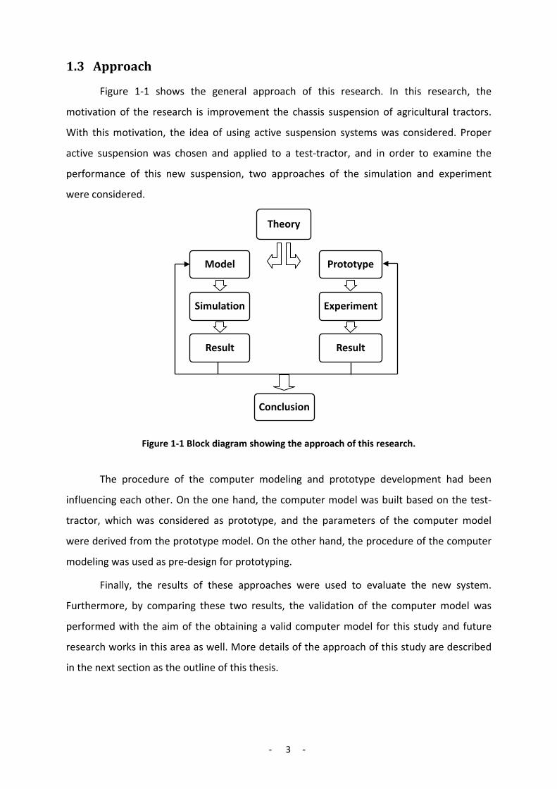
1.3 Approach

Figure 1-1 shows the general approach of this research. In this research, the

motivation of the research is improvement the chassis suspension of agricultural tractors.

With this motivation, the idea of using active suspension systems was considered. Proper

active suspension was chosen and applied to a test-tractor, and in order to examine the

performance of this new suspension, two approaches of the simulation and experiment

were considered.

Figure 1-1 Block diagram showing the approach of this research.

The procedure of the computer modeling and prototype development had been

influencing each other. On the one hand, the computer model was built based on the test-

tractor, which was considered as prototype, and the parameters of the computer model

were derived from the prototype model. On the other hand, the procedure of the computer

modeling was used as pre-design for prototyping.

Finally, the results of these approaches were used to evaluate the new system.

Furthermore, by comparing these two results, the validation of the computer model was

performed with the aim of the obtaining a valid computer model for this study and future

research works in this area as well. More details of the approach of this study are described

in the next section as the outline of this thesis.

Conclusion

Theory

Prototype

Experiment

Result

Model

Simulation

Result

- 4 -

1.4 Outline

In order to achieve the objectives of this investigation, five steps were performed. In

harmony with these steps, this thesis is organized in seven succeeding chapters. These steps

and the relevant chapters are presented here in this section.

The first step of the study was the background and literature review of the

investigation. This was made in the subjects of the suspension system of vehicles and

agricultural tractors, active suspensions, control strategies, and hydro-pneumatic

suspensions. These subjects are presented in the chapter 2 of this thesis. First, general

definitions about vehicle suspension are presented. After that, different kinds of active

suspensions and some related control-strategies are explained. Then, the actuator system of

semi-active suspensions, and the hydro-pneumatic suspension are described. At the end of

this chapter, different kinds of suspension systems used for agricultural tractors are

discussed. Among these subjects, some details on the objectives of the research are also

discussed. This study leads to determine a proper type of active suspensions and control

strategies used for agricultural tractors. Also in this step, the specifications of a test-tractor

used for the experimental study are revealed.

The second step was designing and modeling of a new suspension system. The

modeling included the mathematical modeling, derived from a physical model and finally a

computer model using MATLAB-Simulink program. These subjects are presented in chapter 3

of this thesis. At first, the model of the full suspension tractor is derived. After that, modeling

of the hydro-pneumatic rear suspension is done. This includes also the model of the

actuator. Next, the model of the control system is presented. At the end of this step, the

overall model involving all sub-models is completed.

The third step was the development of the prototype of the suspension system. The

prototype was used for the experimental study of this research. This step is described in

chapter 4 of the thesis. At first, the control system, including hardware and software

components is explained. The controller was a personal computer with proper software. This

computer was connected to the system’s inputs (i.e. sensors) and outputs (i.e. actuators) by

using an interface card. After the control system, the building the hydraulic actuator system

and relevant installation on the hydro-pneumatic rear suspension of the test-tractor is

presented.

- 5 -

The fourth step was the test design and test setup. The test design was similar for the

simulation and experimental tests. It included the determination of the test input, which

used for the excitation of the suspension, and the test output, which used for the derivation

of the test results. Unlike the test design, the test setup of the simulation and experimental

tests were different. For the simulation test, a MATLAB m-file program was used to conduct

the simulation process. For the experimental tests, the suspension test rig at the TU Berlin -

Department Machinery System Design was employed in order to apply the test input to the

tractor. In addition, a data acquisition system attached with acceleration sensors was used in

order to save the output parameters of the test.

In chapter 5 of this thesis, the fourth step of the study is presented. This step is the

test design and test setup. At the first part of this chapter, the test input and output, and the

analysis methods of the output date are determined. Then the test setup of the simulation

tests and the test setup of the experimental tests are presented separately. For the

experimental test, a suspension test rig and a data acquisition system were used. These

equipments are described at the end of this chapter.

The fifth step was the study of the results of the simulation and experimental tests.

These results were derived from the amplitude and frequency based data analysis. By

comparing the simulation results with experimental results, the validation of the model was

performed. After that, performance of the semi-active suspension was investigated by

comparing the passive and semi-active results. Two series of the results related to the

tractor body acceleration and the tire dynamic force were used in order to illustrate the ride

comfort and handling ability of the tractor. At the end, all results were used in order to

determine the conclusion of this study and provide some recommendations for future

works.

The results of the tests are presented in chapter 6. At first, the results of the model

validation are given. After that, two series of the evaluation results related to the ride

comfort and handling of the tractor are presented. Finally, in chapter 7 the results of this

study are concluded. The highlights, significant results, and the summary of the main works

are presented. At the end, recommendations for future work are given.

- 6 -

Chapter 2

2 Background and Literature Review

In this chapter the background of this investigation and the literature review are

presented. At first, general definitions related to vehicle suspensions such as ride comfort,

handling, and passive suspension are described. Then active suspensions and different types

of them are explained. It follows a description of the control strategies for semi-active

suspensions. These suspensions are the systems that were selected as the proper active

suspensions in this investigation. On the other hand, this new system was applied to a hydro-

pneumatic suspension. These suspensions are explained in this chapter. As the final point,

the different types of suspension systems of agricultural tractors are described.

2.1 Vehicle Suspension

On a road with smooth surface, there is no need for a suspension system to provide

ride comfort for the passengers of a vehicle. However, there are various types and roughness

of road surfaces in reality, and a suspension system is necessary in order to isolate the

vehicle from the exciting vibrations of the road unevenness. Besides this function,

suspension systems should maintain a permanent contact between tires and road surface so

as to provide good ride stability for vehicle. This ability is particularly important as vehicle is

turning, accelerating, or braking. Briefly, a vehicle suspension provides ride comfort and

driving stability for the vehicle. They are also necessary for protecting the road surface from

excessive tire forces and pavement damage.

The typical construction of the suspension system of a vehicle consists of the

suspension units, which place at the vehicle corners and connect the vehicle chassis to the

vehicle wheels via a linkage system. Each suspension unit is comprised of two basic

suspension elements of the spring and the damper, setting in parallel. Springs absorb the

shock-excitations, which is caused by the road surface roughness. As the suspension meets a

bump, the spring gets compressed and stores the energy of the shock. After that, it expands

and releases the absorbed energy gradually to the vehicle body. On the other hand, the

- 7 -

function of a damper is to dissipate the energy of suspension vibrations. As the suspension

meets a bump, the damper damps directly a part of the shock energy. In addition, it

dissipates the stored energy in the spring. In this way, it controls the action of the springs.

Likewise, springs and dampers control the motion of the vehicle body, caused by driving

maneuvers.

In most of the vehicles, steel springs are used for the suspension system, which

comes in three types of coil, torsion bar, and leaf springs. Pneumatic and hydro-pneumatic

springs are also used in some vehicles. The details of these systems will be described in the

following sections. Dampers in vehicle suspension systems are mostly hydraulic dampers.

The working principle of the hydraulic dampers is similar. As the damper compresses or

expands, a hydraulic fluid is forced through a throttle. The created pressure-drop in this

throttle creates the damping force. The size of the throttle determines the damping

coefficient of these dampers.

In the following sections, ride comfort and vehicle handling as the two main functions

of the suspension systems will be described. In addition, the limitations of the conventional

suspensions in achieving these functions, and available solutions will be discussed.

2.1.1 Ride Comfort

Ride comfort is considered as the first objective of the suspension systems of

vehicles. Ride comfort is an important characteristic of vehicles that indicates how much

riding is comfortable for passengers. Ride comfort is very important for agricultural tractors,

because the acceleration transmitting to the driver compared with other vehicles is very high

(Horton & Crolla, 1984). In addition, the operators of agricultural tractors spend many hours

in the field during peak working seasons. These conditions can affect the comfort, efficiency,

alertness, and health of the operators.

Vibration sources that affect ride comfort are categorized generally into two classes,

namely on-board sources and road sources (Jamei, 2002). On-board sources arise from the

rotating components including the wheels, the driveline, and the engine. These sources

caused aural vibrations in the frequency region of 25 - 20,000 Hz, which are called "noise"

(Gillespie, 1992). These two frequencies are the lower and higher frequency thresholds of

human hearing. The second category of the vibration sources of vehicles is the road source,

refering to the road roughness and maneuver excitations. Frequency range of these

- 8 -

excitations is between 0 and 25 Hz. This range including the natural frequencies of human

tactile and visual is the most sensitive frequency areas to human body. For that reason, the

road excitation source is considered as the most important factor in affecting ride comfort of

a vehicle.

Suspension systems are considered as the foundation of vehicles ride comfort. The

frequency area of suspension systems is in the range of lower than 25 Hz. In the case of

vehicle dynamics, "ride comfort" is related to only this part of the frequency range (Gillespie,

1992). Ride comfort depends particularly on the dynamic behavior of the vehicle body (i.e.

sprung mass). Vibrations on the body of a vehicle are the combination of the vertical

vibration of heave, and the angular vibrations of pitch and roll.

The vibration effect on human body, particularly about the passengers of a vehicle,

have been examined in many investigations (Bastow, 1987). The human body shows

different sensitivity to vibrations. This sensitivity is dependent on the direction and

frequency content of vibrations. In general, the human body is more sensitive in horizontal

directions compared with the vertical direction. In the vertical direction, the most sensitive

range of the body is 4 - 8 Hz corresponding to the resonant frequencies of the organs in the

abdominal cavity. The sensitivity in the horizontal directions is highest in the range of 1 - 2 Hz

(SAE, 1992). The range 0.5 - 0.75 Hz can be also associated with motion sickness or

“seasickness” (Barak P. , 1991). As a result, the most uncomfortable frequencies to humans

and those that a suspension system needs to control are in the 0.5 - 10Hz range (Barak P. ,

1991). Based on this conclusion, performance of the suspension system in this thesis was

evaluated in the mentioned frequency range.

In order to quantify the ride comfort of a vehicle, vibrations of the vehicle body

should be measured in two directions of vertical (i.e. heave) and horizontal (i.e. roll, pitch

and yaw). The most commonly used measurement methods is the RMS acceleration. Root

Mean Square (RMS) acceleration is defined as:

∫=T

dttaT

aRMS0

2 )(1)( 2-1

With (T) being the total sample time, (a) the sprung mass acceleration, and t the

time. This measurement must be performed for both directions. However, to simplify the

measurement, just the body vertical acceleration (i.e. heave) is often measured. In this

- 9 -

study, in order to evaluate the ride comfort, the RMS accelerations of both the vertical and

horizontal directions were measured. More detail will be presented in chapter 5.

With the purpose of considering the factor of vibration frequency in ride comfort

measurement, a weighted form of accelerations can be used in equation 2-1 instead of the

plain acceleration. In this method, a weighting curve, which is created base on the human

sensitivity of different vibration frequencies, determines a weighting factor for the amplitude

of each acceleration data respect to the frequency of this acceleration data. More detail in

this subject can be found in the reference of (Thoresson, 2003). In another method, with the

aim of considering the frequency factor, the acceleration data of the sprung mass is filtered

by a Human Response Filter (i.e. HRF) (Donahue, 1998).

In general, the mentioned formulation of the RMS acceleration is used in order to

evaluate the ride comfort capability of the suspension systems. The focus of some studies is

the human exposure to the vehicle vibrations. For these studies, other methods are needed

to involve some related variables in measurement of ride comfort. The important variables

are the magnitude, frequency, direction, and duration of vibrations. For example, There are

some standards defined concerning with the measurement of ride comfort of agricultural

vehicles and the acceptable levels of the acceleration transmitted to their operators. Among

them two ISO standards are usually preferred for the agricultural vehicles (Adams, 2002).

The first standard is ISO 2631, which was initially issued in 1974. This standard is a

general norm used for three main issues of vibration measurement, human exposure to the

whole body vibration, and acceptable vibration levels relative to the health risk (Pickel P. ,

1993). In this standard, a vector is used as the weighed factor for evaluating the total load,

which contains the loads of vibrations in all three linear directions (Hansson P. A., 1995). In

addition, this standard considers the factor of time limitation in order to define the

acceptable vibration levels of human.

Another standard is ISO 5008 issued initially in 1974. This standard describes a

method for the measurement and analysis of the vibration load on the driver of an

agricultural tractor (Hansson P. , 1995). This standard presents a rough and a smooth test-

track, which are designed in order to imitate normal driving conditions in agricultural

applications. In addition, ISO 5008 recommends that the test-tracks should be traversed at 5

km/h and 12 km/h (Adams, 2002). This standard makes use of the ISO2631/1 standard in

order to weight the frequency information of accelerations. Then, it integrates the values

- 10 -

overall frequencies in order to form a single root mean square (RMS) value for acceleration

(Adams, 2002).

2.1.2 Vehicle Handling

Handling is a characteristic of a vehicle that provides stable and safe driving that can

be created via a steady contact between the tires and road surface. In some references,

handling is called also with other names such as road holding, ride stability, and driving

safety, implying the same meaning. The handling capability of a vehicle is important during

maneuvers such as cornering, braking, or accelerating. In these extreme situations, weak

handling reduces the control ability of the vehicle and can affect the safety of the

passengers. Due to this fact, handling is considered as an important capability for vehicles,

and beside the ride comfort, it is considered as the main target of using the suspensions in

vehicles.

Handling is related to the tire contact force that is influenced by two factors: wheel

and vehicle body vibrations. Vertical motion of the wheels is affected mainly by road

roughness, and body motions are produced mainly by vehicle directional changing. The

maneuvers changing of vehicles are considered as the major challenge for the handling

characteristic of a vehicle. For example during cornering, the centrifugal forces push vehicles.

This must be resisted by the tire contact forces. In the same time, the centrifugal force

causes load shift on the tires from one side of the vehicle to another side. This leads to major

reduction in the tire contact forces and provides consequently a poor handling performance.

Likewise, as a vehicle brakes or accelerates rapidly, a critical handling state is created. In this

condition, extra traction forces on the tires are needed, whereas because of the weight

transfer from back to front or conversely, tire contact force cannot be created optimally.

The handling capability of a vehicle is affected by different characteristics of the

vehicle. The main one is the characteristic of the vehicle suspension. A good suspension

provides strong resistance to the vehicle body motion (i.e. roll, pitch and heave) and

prevents excessive weight transfer in the vehicle body, which increase the vertical loads of

the wheels and affects the handling negatively. In addition, an effective suspension can

control the vertical vibration of the wheels (i.e. wheel hop), which are produced by the road

roughness and have direct influence on the tire contact force and consequently on handling

of the vehicle.

- 11 -

As mentioned above, vehicle handling and ride comfort are the two main functions of

the vehicle suspension. In order to evaluate a suspension system, these two characteristics

must be measured and examined. Unlike ride comfort, which was explained before, there is

no standard to quantify or formulate the vehicle handling. This makes the qualification of the

handling complicated. However, there are some methods for indirect measurement of

handling. Good handling can be provided by stable tire contact forces, and high variation of

the tire force reduces the handling capability of the vehicles.

As a result, variation of the contact force between the tires and road surface

corresponds directly to the vehicle handling, and it can be used for the quantification. The

term of tire contact force is equal to the vertical tire force. As a result, the tire force variation

or dynamic tire force can be used in order to measure the handling. Lower dynamic tire force

means better handling and higher dynamic tire force indicates worse handling. In

experimental works, the direct measurement of the vertical tire force is difficult. Measuring

the deflection of tires is often an alternative. Due to the elasticity of tires, this deflection is

proportional to the vertical tire force.

(Mitschke, 1984) defined a factor called RLF “Radlastfaktor” in order to quantify

vehicle handling. In calculating this factor, the vertical static tire force was considered in

addition to the vertical dynamic tire force. RLF factor is equal to the value of the dynamic tire

force over the value of the static tire force. Greater value of this factor means higher

instability in the tire contact, implying worse handling. In another related study about tractor

dynamics, RLF factor was used also for examining handling of tractors. The conclusion of this

investigation is that the handling of tractors is acceptable if the RLF value is lower than 0.33

(Ulrich, 1983). This factor was also used by (Hoppe, 2006) in order to evaluate the handling

capability of a full suspension tractor.

Handling capability for the agricultural tractors is particularly important. A

comparison of agricultural tractors with automobiles shows that the position of the center of

gravity is higher. Further differences are the higher body mass and the lacking chassis

suspension. As a result, tractors have normally poor roll and pitch stability. In extreme

situations poor handling may lead to very weak steering and braking control ability of the

vehicle. On the other hand, effective agricultural processes need a higher tractor velocity.

This demand leads to an increasing importance of the handling capability for agricultural

tractors.

- 12 -

In the investigation of (Simon, 2001), it was concluded that the limit of the handling

performance of automobiles is characterized by the loss of the yaw stability, whereas this

limitation in off-road vehicles should be characterized by the loss of the roll and pitch

stability. In this investigation, the main objective was improvement of the tractors handling.

It was concluded that this can be achieved via providing a better control on the vibrations of

the tractor body (i.e. roll, pitch, and heave) by using an effective chassis suspension for the

tractor.

2.1.3 Passive Suspension Compromise

Usual suspension systems of vehicles are passive suspensions. In these systems, the

characteristics of the suspension elements are constant. In the design of these systems,

there is an inherent compromise between good ride comfort and vehicle stability as the two

main goals of the design. A vehicle suspension with stiff spring and firm damper is referred

as 'hard' suspension. This provides good control on the vehicle body motion and wheels

vibration, and it creates optimal handling. However, this system is unable to offer effective

body isolation. On the other hand, a suspension with low stiffness and soft damping, called

'soft' suspension provides effective body isolation from road unevenness and creates good

ride comfort. However, this system cannot control the motions of the vehicle body and

wheels effectively. Therefore, in the design of conventional passive suspensions, a

compromise has to be made between good handling and ride comfort. This limits the

performance of passive suspensions.

Figure 2-1 indicates the compromise in suspension design due to the damping ratio.

In suspension design, the main way to specify the suspension is the tuning of the damping

rate, because the selection of the spring stiffness is generally based on the vehicle’s weight.

A suspension with high damping ratio damps the resonance of the sprung mass effectively.

However, it increases the transmissibility of the road roughness and provides a poor ride

comfort for the vehicle. Conversely, low damping ratio decreases the transmissibility of the

road roughness. However, it is not able to damp the resonance of the sprung mass

effectively and provides a poor handling capability.

- 13 -

Figure 2-1 The compromise present in passive suspension design.

Even a good design for passive suspensions cannot remove this trade-off, but also it

can only optimize one set of the driving conditions. For example, sports cars with a hard

suspension provide a good handling capability and safe fast cornering, which is achieved at

the cost of relative uncomfortable ride for driver. Conversely, city buses with a soft

suspension provide a comfortable ride for passengers achieving at the cost of having poor

handling capability. Therefore, designers must decide about the priority of ride comfort or

handling based on the purposed application of the vehicle.

In order to overcome against the drawback of passive suspensions caused by the

inherent compromise, active suspensions are considered as the key of this problem,

presenting the possibility of optimizing both ride comfort and handling. These systems will

be described in the following sections.

2.2 Active Suspension

In a passive suspension system, springs store and dampers dissipate the energy of the

vibration. The parameters of these elements are generally fixed and are chosen in order to

achieve a certain level of the compromise between road holding and ride comfort of the

vehicle. This compromise limits the performance of the passive suspension. In order to

eliminate this limitation, other types of suspensions with beyond the passive components

are expected. Advance in electronic technology has recently provided new facilities for

improvement in the suspension of vehicles.

Modern suspensions are equipped with electronic control systems that control the

operation of the suspension elements. They have not a limited performance like passive

suspensions and create a new advancement in removing the drawback of the design

compromise present in passive suspensions. This optimizes both the ride comfort and

- 14 -

handling capability of vehicles. Therefore, active suspension systems are considered as a

proper solution in order to increase the performance of conventional suspensions and create

an effective suspension for vehicles. The idea of active suspension has been also considered

in this investigation with the aim of improving the performance of the chassis suspension of

agricultural tractors. The term of “active suspension” is used in this thesis for referring to

each type of the modern suspension that uses an electronic system for controlling the

suspension. These systems are different from passive systems that have constant

characteristics.

There are different types of active suspension. They could be relative simple such as

manual adjustable systems or relative complicated such as fully automatic systems. They

may use open loop controls or use sensory feedback loop controls. Their bandwidth could be

low, covering a part of the suspension vibrations, or it could be relative high, covering all the

suspension vibrations. They could work just by dissipating the suspension energy or work by

consumption of extra energy. In this script, all these advanced suspension systems are

classified to the four categories: adaptive, load leveling, semi-active, and fully active

suspension. Each one will be described in the following sections. In addition, these

suspension systems will be compared to one another in order to choose the proper system

for the chassis suspension of agricultural tractors.

2.2.1 Adaptive

In the design of passive suspension systems, there is an inherent compromise

between ride comfort and handling as two main design goals. The priority of these two goals

of suspensions is dependent on the operation conditions of the suspension. For example, as

a vehicle is driving on a rough road, ride comfort should be considered as the priority of the

vehicle suspension. On the other hand, as the vehicle arrives to a smooth road with many

corners, the priority shifts to handling rather than ride comfort. Therefore, a suspension

system that can adapt its parameters to the different operation modes is able to offer an

efficient performance. This system is called adaptive suspension system. They work normally

alike a passive system, until a change in operating condition of the suspension appears. This

system recognizing the change modifies the parameters of the suspension respect to the

change and adapts the suspension to the new condition.

- 15 -

In simple type of adaptive suspensions, change in operation condition of the

suspension is recognized directly by the driver of the vehicle, and the modification in the

suspension parameters is also performed directly by the driver manually. Figure 2-2

illustrates one of these systems that let driver choose one of three suspension modes of

“soft”, ”medium”, and “firm”. These modes are in fact three damping levels for the

suspension. For example, driver can choose the soft suspension mode as the vehicle is

running on a rough road. This provides a better ride comfort capability. In contrast, during

driving on a highway at high speed, firm suspension mode can be selected in order to

provide better ride stability. Advantage of these systems is the considering of the driver

impression. However by such a manual system, fast control cannot be provided, and proper

reaction to the short time changes in the operating condition of the suspension is

impossible. Therefore, instead of manual control, the automotive control systems are

employed in the advanced adaptive suspensions.

Figure 2-2 A system of manually adjustable dampers for vehicle suspension (Barak P. , 1989).

In automotive adaptive systems, the operating condition of the suspension is

distinguished based on the sensory information. After that, controller accomplishes the

necessary change in the suspension parameters. There are different ways for detecting the

operating condition of a suspension. In one system, the driver commands such as gas, brake,

and steering commands are measured. The achieved signals are used as the inputs of

adaptive control, and based on them; the controller can recognize the maneuver conditions.

For example, intense and frequent driving commands infer a severe maneuver condition.

This condition needs high ride stability, which can be provided by a firm suspension.

rear dampers front dampers

selector

controller

soft

medium

firm

- 16 -

In another type of adaptive systems, the maneuver condition and road surface

quality are recognized by analysis of the accelerations of the vehicle which are measured by

proper accelerometers. The amplitude and frequency analysis of the vertical, longitudinal, or

lateral accelerations are considered. The analysis can be also performed based on the

suspension deflection of the vehicle (Lizell, 1990). In some other systems, the travel speed of

the vehicle is measured as input of the adaptive control. High speed driving on the straight

and even roads implies the need to better ride stability, which can be provided by high

handling capability of vehicles (Williams, 1994).

The output of an automatic adaptive suspension is indeed to make the proper

changes in suspension parameters. Similar to the manual system, this is performed often by

changing the damping level of the suspension. However, the output of a type of these

systems is the stiffness of the suspension. In this system, which is called load-leveling

system, the stiffness is determined based on the static load of the vehicle. The details of this

system will be described in the next section.

For an adaptive suspension system, just a low bandwidth for the controller is needed,

because an adaptive suspension system reacts only to the steady form of the changes in

operating condition of the suspension, for example, entering of a vehicle from a smooth road

to a rough road. In the new adaptive systems, the bandwidth of the controller is increased in

order to create the ability of fast responding to the suspension inputs such as a bump or

sudden brake. However, the bandwidth of these systems is still lower than the natural

frequencies of the vehicle body, and their performance is limited. Higher control bandwidths

are used in other types of active suspension systems such as semi- active and fully active

suspension systems. These systems will be described in the next sections.

In the study of (Karnopp & Margolis, 1984) , a fast adaptive system was investigated.

Quick changes was performed in suspension parameters of the hydro-pneumatic suspension

system of a vehicle. This performed on both the damping and stiffness level. The input of the

control system was the frequency response of the vehicle body vibration. Examination of this

system showed the high potential of this system in improving both the ride comfort and

handling of the vehicle.

Adaptive suspension systems have a high potential for agricultural tractors. These

vehicles works in a wide range of different operating conditions from the field work to the

driving on the normal asphalt roads. By using adaptive suspension, the suspension

- 17 -

parameters can be tuned proportional to different conditions. This provides an efficient

suspension for tractors in all working conditions.

2.2.2 Load Leveling

Normally, static changes in the load of vehicles create steady changes in the vehicle

height, which is unwanted. A load leveling control system provides a constant vehicle height

in spite of these changes. This system detects the changes and tunes the springs’s stiffness of

the vehicle proportionally in order to correct the suspension height, and in this way, the

vehicle height stays invariable. These systems react only to the static inputs and have a low

control speed, but they still provide noticeable benefits for vehicle suspensions and improve

their performance. The advantages of load leveling control systems can be stated as follow:

1- In a passive suspension, until 50% of the suspension strike may be absorbed after

increasing the vehicle load, and just remained value can be used against dynamic inputs

from the road. While by using load-leveling system, the whole suspension strike stays usable

despite the different static loads (Eulenbach, 2003).

2- In a passive suspension, considering the maximum static loads, relative hard

springs are used. This reduces ride comfort of vehicles, particularly as a vehicle is running

with a low value of loading. Whereas by using load leveling system, softer springs can be

used in the suspension. These springs can be until six times more flexible than conventional

suspension and provide obviously better ride comfort for the vehicle (Williams, 1994).

3- In principle, the natural frequencies of the body of vehicles depend on the vehicle

load and suspension stiffness. The stiffness is constant in a passive suspension. As a result,

with change in the vehicle load, the natural frequencies of the vehicle body are changed.

This affects negatively the suspension performance and decreases ride comfort and handling

capability of the vehicle. While using a proper load leveling system, the spring’s stiffness is

tuned proportional to the change in the vehicle load. In this way, the dependency of the

vehicle natural frequencies to the vehicle load is nearly eliminated, and the suspension

performance is improved consequently.

Load leveling controller is a sensory feedback loop controller, which uses

displacement sensors for measuring the suspension height. The signals of these sensors are

passed first through a low-pass filter in order to remove the signals related to the dynamic

changes in the suspension height. In this way, the static suspension height is just used as the

- 18 -

input of control. The load leveling control system responses just to the static changes of the

suspension height, and it has a low speed controller. In practice, the bandwidth of this

system is usually less than 0.25 Hz (Burton, Truscott, & Wellstead, 1995). This low bandwidth

leads to an uncomplicated construction and low energy consumption of this system. These

facts have converted the load leveling system to the most practicable active suspensions in

vehicles (Williams, 1994).

The load leveling control is especially practicable by pneumatic and hydro-pneumatic

suspension systems. In these systems, the stiffness can be adjusted by charging and

discharging oil or air to the system, which leads to correct the suspension height. These

systems need an external power source to drive oil or air pump to the system. This power

source is provided from the vehicle engine. However, there are also self-energized systems

using relative suspension movement to pump oil to the system (Meller, 1987).

The load leveling system keeps the suspension height in a constant primary value. By

adjusting of this value with respect to the driving condition, operation of the suspension can

be developed. This can be performed manually by driver or automatically by a control

system. The automatic system uses sensory information to recognize the driving condition

and determine the proper primary suspension height. For example, as a vehicle is driving

with high speed on a flat highway, the center of gravity of the vehicle can be shifted lower by

reducing the primary height. This improves ride stability of the vehicle. In addition, the

aerodynamic resistance of the vehicle is decreased (Giliomee, 2003). On the other hand,

driving on uneven roads needs a higher suspension height to prevent hitting of the chassis

with the road surface.

Load-leveling systems have been used widely for heavy vehicles that work usually

with a wide range of load variation. A group of these vehicles is agricultural tractors that

have great potential to benefit from load leveling systems. A load leveling system used for

the front axle suspension of an agricultural tractor was described in the investigation of

(Marsili, Ragni, Santoro, & Servadio, 2002). This system was adjusted so as to react only to

the more than 2cm change in the suspension height. The change had to be survived for at

least 3.5 second. This proved that the change was a static type.

An example of manufactured tractors using this system is “Fastrac” from “JCB”

Company. This tractor is a full suspension tractor with the hydro-pneumatic rear suspension

that is equipped with a load leveling control system. Figure 2-3 illustrates the working of this

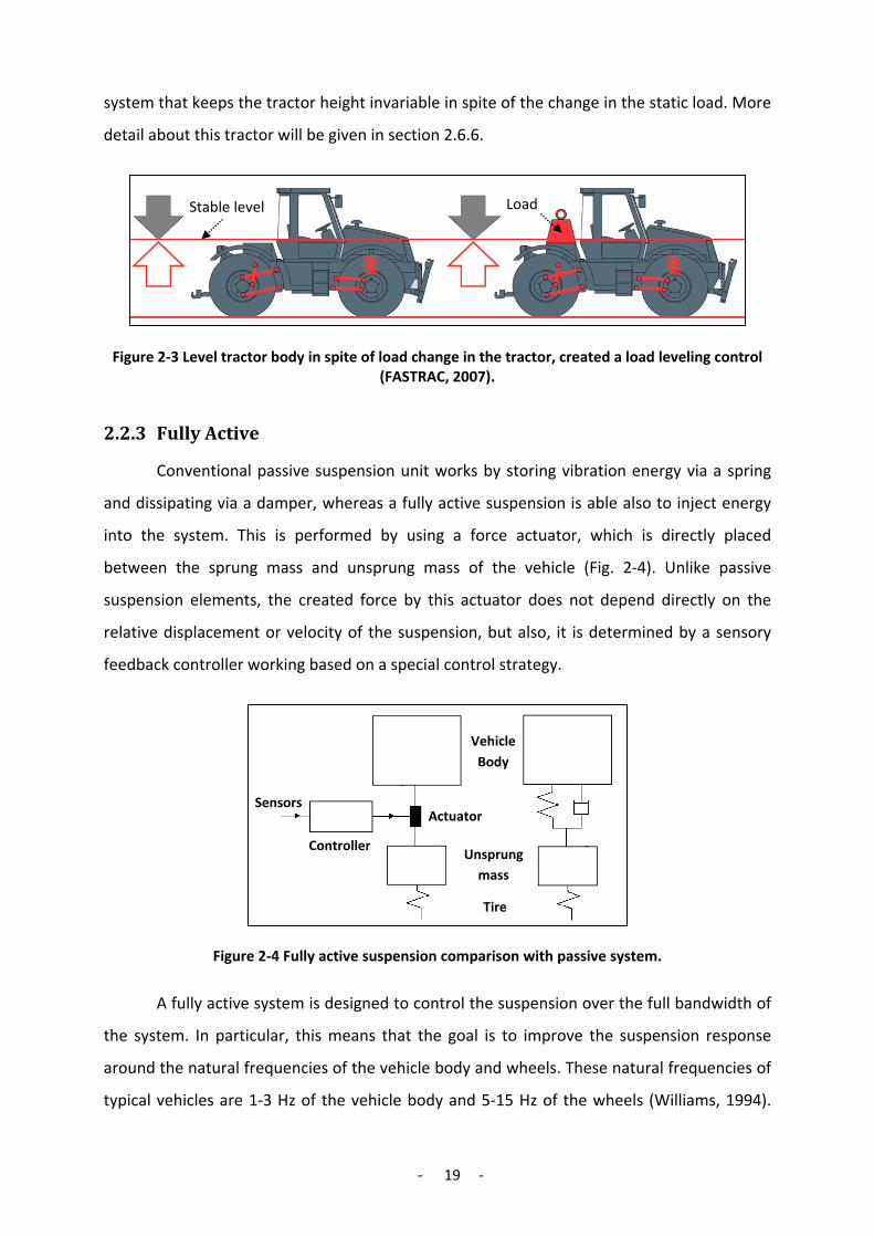
- 19 -

system that keeps the tractor height invariable in spite of the change in the static load. More

detail about this tractor will be given in section 2.6.6.

Figure 2-3 Level tractor body in spite of load change in the tractor, created a load leveling control (FASTRAC, 2007).

2.2.3 Fully Active

Conventional passive suspension unit works by storing vibration energy via a spring

and dissipating via a damper, whereas a fully active suspension is able also to inject energy

into the system. This is performed by using a force actuator, which is directly placed

between the sprung mass and unsprung mass of the vehicle (Fig. 2-4). Unlike passive

suspension elements, the created force by this actuator does not depend directly on the

relative displacement or velocity of the suspension, but also, it is determined by a sensory

feedback controller working based on a special control strategy.

Figure 2-4 Fully active suspension comparison with passive system.

A fully active system is designed to control the suspension over the full bandwidth of

the system. In particular, this means that the goal is to improve the suspension response

around the natural frequencies of the vehicle body and wheels. These natural frequencies of

typical vehicles are 1-3 Hz of the vehicle body and 5-15 Hz of the wheels (Williams, 1994).

Load Stable level

Controller Unsprung

mass

Actuator

Vehicle Body

Tire

Sensors

- 20 -

These systems cover the full bandwidth of the suspension system and are able to perform a

complete control on the vibrations. This provides good ride comfort and road stability for

vehicle. However, the high bandwidth control leads to a significant quantity of power

consumption, which is approximately until 10 kW for the normal automobiles. This high

power consumption can affect negatively the overall performance of the vehicle and

increases the fuel consumption in the range of 10 – 15 % (Williams, 1994).

On the other hand, the high bandwidth of these systems means that more accurate

and faster components especially wide bandwidth actuators are required. This leads to the

relative complexity and high expense of these systems. The relatively high level of noise is

another weakness of these systems due to the disability in isolating the high frequency

vibrations. These systems generate themselves also undesired noise causing from the fast

action of their actuators. This affects negatively the ride comfort of the vehicles. However,

this problem can be reduced by placing rubber elements in series with the actuators in the

system.

Since in a fully active suspension, the passive suspension elements are replaced by an

actuator, the actuator force has a central role in suspension performance. In this condition,

the failure modes of the actuator can affect critically the suspension. For example, an error

in operation of the controller in determining the actuator force may cause a major failure in

producing damping or stiffness force in the system. This leads to a major drop in ride quality

and road handling of the vehicle. On the other hand, a strong wrong force by an actuator

may cut the tire contact from the road surface and reduce critically the stability and

controllability of the vehicle. Such situation may lead to create dangerous modes for vehicle

and passengers.

Considering these weaknesses of fully active suspensions, in spite of the high

performance of these systems, they are not used generally for the normal vehicles, and just

for luxury or special vehicles are employed. In order to have a more practicable system of

the fully active suspension, low-bandwidth type of these systems is presented. In this

system, the actuator is placed in series with a passive spring and, in some cases, in series

with a passive damper (Fig. 2-5). Unlike fully active system, this system is not designed to

control the suspension vibrations over the full bandwidth of the system. On the contrary, the

goal is to improve the suspension response just around the natural frequencies of the body

of vehicles, with the typical range of 1 – 3 Hz, because these frequencies area has the main

- 21 -

role in both ride comfort and handling of vehicles. At higher frequencies, the actuator does

not work effectively, and the wheel-hop motion is controlled only by the passive elements.

Figure 2-5 Configuration of a low-bandwidth active suspension (Williams, 1994).

In practice, in spite of the lower bandwidth, performance of the low-bandwidth

active suspensions is relative similar to fully active systems in providing good ride quality and

handling capability for vehicles (Williams, 1994). These systems are able to create significant

reduction in the body roll and pitch motions during vehicle maneuvers such as cornering and

braking. This efficiency is achieved with lower energy consumption than high bandwidth

systems. In addition, since in these systems, passive suspension elements are employed

beside the actuator, the failure modes in system are not critical such as high-bandwidth

systems. These capabilities of these active systems have led to their application for

automobiles. The major motor manufacturers, such as Jaguar, BMW, Mercedes Benz, and

Toyota have already presented their own fully active suspension systems.

Many research works have been already conducted in this area with the purpose of

performance evaluation of fully active suspensions. One of these investigations is the basic

research work of (Chalasani R. , Dec.1986) that applied a low-bandwidth active suspension to a

quarter-car model. He examined the suspension system by using white noise as the road

input of the suspension. After the examination, he concluded that the RMS value of the

sprung mass acceleration was 20% reduced in comparison with a passive system. This was

achieved without negative effect on the unsprung mass vibration and suspension travel.

Power consumption of low-bandwidth fully active systems is lower than the high-

bandwidth systems. However, this consumption is still considerable, especially about heavy

Tire

Body

Sensors

USM

Actuator

Controller

- 22 -

vehicle. In the research work of (Deakin, Crolla, & Shovlin, 1997), the power consumption of a

military heavy vehicle, equipped with low-bandwidth active suspension, was examined. The

result of this investigation showed that until 25 % power of the vehicle engine could be spent

for the active suspension. However, this value for smooth roads was just 3 %. In a similar

investigation (Donahue, 1998), a low-bandwidth active suspension was applied to a military

off-road heavy vehicle “HMMWV”. The tests showed that until 30 HP of 150 HP engine

power was used by the active suspension. This led to considerable increase in the fuel

consumption of the vehicle.

Fully active systems provide high performance, but they are not used for the chassis

suspensions of the heavy vehicles such as agricultural tractors. Fully active systems in these

high masse vehicles consume considerable energy. However, for the partial suspension of

heavy vehicles, the fully active systems have been already used successfully. For example,

these systems have presented a good efficiency in the seat and cabin suspension of tractors.

2.2.4 Semi-Active

In a fully active suspension, a force generator using extra energy source is put in the

passive suspension with the purpose of improving its performance. In a semi-active

suspension, the active force generator is replaced with an adjustable damper. Using this

damper, the rate of energy dissipation can be changed depending on the instant condition of

the suspension motion. Figure 2-6 shows the construction of a semi-active suspension. In

this suspension, the passive damper is replaced with an adjustable damper that its damping

rate is determined by a controller with closed loop control, using sensory information as

feedback.

Figure 2-6 Semi-active suspension system.

- 23 -

In order to clarify the difference between the operation of semi-active and fully

active suspensions, the working area of these two systems are illustrated in figure 2-7. In a

fully active system, the four operation areas are covered, because the force of the actuator

can be applied to the system in direction or against the direction of the suspension

movement. In spite of this, in a semi-active system, the force of the adjustable damper can

be applied to the system only against the direction of the suspension movement. Thus, just

two areas of the four operating areas are covered by this system.

Figure 2-7 Working area of the semi-active and fully active suspensions.

Basic theory of a semi-active suspension is the controlling of the damping level of the

suspension. However, there are different strategies to perform this control. A semi-active

control approach determines the damping level based on the sensory information. These

strategies will be described in the next sections.

The main difference in the construction of a semi-active suspension with a fully active

suspension is the actuator of the system. The actuator of a semi-active suspension is in fact a

controllable damper with a relative simple construction in comparison with the force

actuator of a fully active system. A controllable damper is made normally based on the

common hydraulic dampers. In these dampers, the damping force is created based on the

throttling the hydraulic fluids. Two main methods are used in order to control the damping

rate of the controllable dampers.

In the first method, the controlling of the damping rate is created by adjusting the

cross area of a throttle. The hydro-pneumatic suspensions are the proper systems for

performing this method, because they can be equipped with a controllable throttle-valve

between the cylinder and accumulator (Fig. 2-8). This method was used in this investigation

as the actuation system of a semi-active suspension. More details about these systems will

be presented in the next parts.

- 24 -

Figure 2-8 A hydro-pneumatic suspension as a semi-active suspension by using a controllable throttle.

The second method for creating a variable damper is based on the viscosity property

of the hydraulic oil instead of cross-area of the throttle of a damper. There are two kinds of

such fluids. The first one is electro-rheological (ER) fluid. Viscosity of this fluid can be

changed by electrical field. The second fluid-type is magneto-rheological (MR) fluid. Viscosity

of this fluid can be controlled by magnetic field. A schematic illustration of a controllable

damper working with the MR fluid is shown in figure 2-9.

Figure 2-9 Schematic Illustration of a MR damper (Paré, 1998).

Advantage of these MR dampers is in their high-speed response, which is in the range

of millisecond. This is important in a semi-active control system, because among all

components of this control system, the time response of the actuator is the most limiting

factors in order to create the proper control bandwidth (Mäkelä, 1999). A feature of these

dampers is their form and their dimension that is similar to the typical passive dampers, and

so, they can be simply installed in their place. MR dampers has priority to the ER dampers in

- 25 -

practicable application (Goncalves, 2001), because they can be directly operated by the

electricity source of a vehicle. In addition, they provide a wide range of damping rate.

Many research works have been conducted about semi-active suspension since its

introducing in early 1970’s. The primary researches investigated this idea theoretically by

using simple car models. Later, the practicable application of the system was also

investigated for the different types of vehicles such as motorcycle, automobile and heavy

vehicle. Some of these research works proved that the performance of semi-active

suspensions can be considerable and competitive with fully active suspensions. For example,

in the analytical investigation of (Margolis D. , 1982), performances of semi-active suspensions

were compared with active suspensions. As result, some control strategies for a semi-active

suspension were presented. With these strategies, the semi-active suspension offered

comparable performance to fully active suspensions. In another research work (Karnopp,

Crosby, & Harwood, 1974), it was concluded that a continuous semi-active suspension can

achieve an acceptable performance near a fully active suspension.

In most of the studies about the semi-active suspensions, the efficiency of this system

are examined only in providing good ride comfort for vehicles. However, because of the well-

known compromise present in the suspension design, the handling of vehicles should be also

examined besides the ride comfort. To be exact, after achieving improvement in ride

comfort, the change in vehicle handling should be studied. In the research work of (Heo, Park,

& Hwang, 2000), both of these two criteria were considered for examining a semi-active

suspension. This suspension was applied to an automobile with some different control

strategies. The results of this investigation showed that this system was able to improve the

ride quality without aggravating the handling capability of the vehicle.

In another research work (Margolis & Nobles, 1991) , it was concluded that by using

semi-active suspensions for heavy vehicles, the vibrations control of the body of these

vehicles such as roll and heave control was improved. In addition, this improvement affected

the handling capability of the vehicles positively. In the work of (Yi & Hedrick, 1993) the

influence of semi-active suspensions on the dynamic tire force of vehicles was investigated.

The dynamic tire-force was considered as the criterion of the handling capability. Using the

prototype of a vehicle, some experiments were performed on a suspension test rig. The

results of these tests showed that improvement in ride comfort of the vehicle was achieved

- 26 -

without rise in the dynamic tire force. In other words, improvement in ride comfort was

accomplished without drop in the handling capability of the vehicle.

Failure modes of semi-active suspension systems are less than fully active systems,

because their operation is simpler. In these systems, just damping force is controllable, and

error modes just lead to create a passive damping mode in the suspension. This decreases its

efficiency without creating a critical situation in the vehicle. Besides this advantage, semi-

active suspensions have low energy consumption, and these systems have not complicated

construction and high cost. These properties beside the notable performance make these

systems as a practicable system and are usually preferred over fully active suspensions.

These semi-active suspensions are considered and employed in the new vehicles by most of

the famous companies.

For the heavy vehicles, semi-active suspensions are preferred particularly as a

practicable way in order to improve their suspension performance (Efatpenah, Beno, & Nichols,

2000). Application of fully active suspensions for heavy vehicles, which have high mass and

inertia, leads to unacceptable high-energy consumption. In an investigation (Nobles & Miller,

1985), efficiency of semi-active suspensions for military heavy vehicles was studied. For this

purpose, a tank was considered, and the four wheels of its ten wheels were equipped with

the semi-active suspensions. Performance of this tank was tested on a virtual road. In this

evaluation, the energy absorption of the body vibration was considered as the criteria of ride

comfort.

The results showed a significant reduction (13-40%) in this criterion, indicating a

significant improvement in ride comfort. An agricultural tractor is also a heavy vehicle used

for agricultural applications. Semi-active suspensions having low energy consumption are

proper systems for these vehicles, especially for the chassis suspension of the tractors.

However, the application of semi-active systems in the chassis suspension is still in research

stage. At this time, the semi-active suspension is used in practice for the secondary

suspension of tractors, such as seat and cab suspension. The proper active suspension for

agricultural tractors that was a key theme in this study will be discussed in the next section.

2.2.5 Conclusion

In this investigation, it was intended to improve the performance of the chassis

suspension of agricultural tractors by way of using active suspensions. This began with

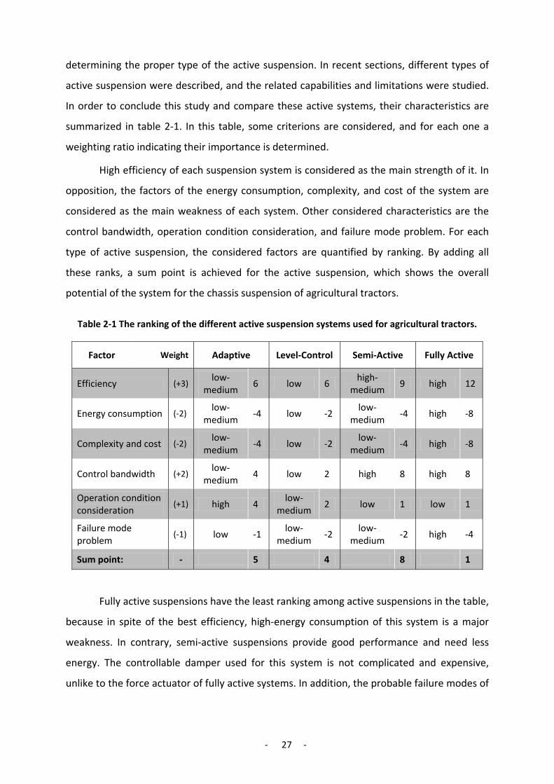
- 27 -

determining the proper type of the active suspension. In recent sections, different types of

active suspension were described, and the related capabilities and limitations were studied.

In order to conclude this study and compare these active systems, their characteristics are

summarized in table 2-1. In this table, some criterions are considered, and for each one a

weighting ratio indicating their importance is determined.

High efficiency of each suspension system is considered as the main strength of it. In

opposition, the factors of the energy consumption, complexity, and cost of the system are

considered as the main weakness of each system. Other considered characteristics are the

control bandwidth, operation condition consideration, and failure mode problem. For each

type of active suspension, the considered factors are quantified by ranking. By adding all

these ranks, a sum point is achieved for the active suspension, which shows the overall

potential of the system for the chassis suspension of agricultural tractors.

Table 2-1 The ranking of the different active suspension systems used for agricultural tractors.

Fully Active Semi-Active Level-Control Adaptive Weight Factor

12 high 9 high-medium 6 low 6 low-

medium (+3) Efficiency

-8 high -4 low-medium -2 low -4 low-

medium (-2) Energy consumption

-8 high -4 low-medium -2 low -4 low-

medium (-2) Complexity and cost

8 high 8 high 2 low 4 low-medium (+2) Control bandwidth

1 low 1 low 2 low-medium 4 high (+1)

Operation condition consideration

-4 high -2 low-medium -2 low-

medium -1 low (-1) Failure mode problem

1 8 4 5 - Sum point:

Fully active suspensions have the least ranking among active suspensions in the table,

because in spite of the best efficiency, high-energy consumption of this system is a major

weakness. In contrary, semi-active suspensions provide good performance and need less

energy. The controllable damper used for this system is not complicated and expensive,

unlike to the force actuator of fully active systems. In addition, the probable failure modes of

- 28 -

a semi-active suspension are not critical. Therefore, semi-active suspensions gain the best

ranking, and they are considered as the proper choice.

The two other systems (i.e. adaptive and load leveling systems) offer acceptable

efficiency, but not as well as the semi-active system. These systems have a ranking between

fully active and semi-active systems. Because of the special function of these systems, they

can be employed beside the semi-active suspension. This is particularly useful for agricultural

tractors that work in wide different operating conditions. Adaptive suspension systems are

able to involve the factor of suspension operating condition, and load leveling control system

can remove the negative influence of the load variation on suspension systems.

2.3 Semi-active Control Strategies

For each type of active suspensions, many different control approaches has been

used. Active suspensions are usually considered as the first practicable system for the

examination of the modern control theories, because a vehicle suspension, with some

simplifications and linearizations, symbolizes a true MIMO-system that its mathematical

model can be simply derived. In addition, ground vehicles are quite familiar example for

people, because almost everybody has an experience with driving an automobile. In most of

the investigations about the modern control theories, a linearized quarter model of the

vehicle suspension is used. By using this model, different control methods and their basic

features can be derived without creating complexity (Elmadany & Abduljabbar, 1999).

The semi-active suspension is the system that was used in this study. Main

practicable control approaches of semi-active suspensions will be reviewed in this part. With

small changes, these methods can be also used for fully active systems. At first skyhook-

based strategies of “skyhook”, “groundhook” and “hybrid” will be presented. After that,

fuzzy control method and preview control method will be reviewed. Finally, the on/off

damping control approach will be described

2.3.1 Skyhook

Skyhook is one of the most famous control methods for active suspensions and is

considered today as a classical method. This method was introduced for the first time in

1974 by (Karnopp, Crosby, & Harwood, 1974). Skyhook was derived by LQR calculation from the

optimal control method, as the control aim was to minimize the RMS value of the sprung

mass acceleration of the suspension. As from the name of “Skyhook” can be realized, the

- 29 -

vibration of the sprung mass in this method is damped by a damper that is connected to a

fixed point in space (Fig. 2-10).

Figure 2-10 Sky-hook damping approach.

Force of the skyhook damper can be defined mathematically as:

2zcF ssky ′= 2-2

However in sky-hook approach, the damper connection to the fixed point can be

performed only in a stationary system. In mobile systems like vehicle suspensions, a force

actuator between sprung and unsprung masses is used to simulate the skyhook damper

force. In a fully active suspension, a force actuator generates the sky-hook force by using an

external power source, whereas in a semi-active suspension, a controllable damper is used

as the force actuator (Fig. 2-11). This damper simulates the skyhook damper force without

using external power source, just by dissipating the suspension energy.

Figure 2-11 Practicable implementation of sky-hook damping approach.

- 30 -

The generated force by the practicable damper with coefficient of c₂ is calculated as:

)( 122 zzcFd ′−′= 2-3

This force must be equal to the skyhook damper. Therefore, considering equation 2-2, the

damping coefficient of the practicable damper can be calculated as:

)()(

12

222122 zz

zcczczzcFF ssskyd ′−′

′=→′=′−′→= 2-4

However, a damper generates the damping force always in inverse direction of the

suspension movement. As this force is not in the demand direction, the damper must be

shut off. The following switching law performs this consideration in the damper equation:

<′−′′≥′−′′′−′

=0)(00)()(

122

122122

zzzzzzzzc

Fd 2-5

Because of the strengths of skyhook control strategy, this method is usually

considered as a reference for evaluation of the other control strategies. However, this

method is not perfect and has some weaknesses. As mentioned, sky-hook method was

derived with the purpose of controlling the sprung mass vibration. In the skyhook

construction, the damper is connected just to the sprung mass, and the control is focused on

it. With this construction, the unsprung mass vibration remains without damping force.

Therefore, reduction of the unsprung mass vibration is achieved at the cost of the

rising sprung mass vibration. In the vehicle suspensions, this problem causes high wheels

bouncing and leads to a poor tire contact with road surface. As a result, this control strategy

is useful when the vibration control of the sprung mass or the ride comfort of a vehicle is in

priority. However, in the practicable implementation of skyhook, the damper is placed

between the two masses, and using this construction, this problem is moderated. This

subject will be discussed in the next chapter.

Another weakness of skyhook strategy is the high level of jerk in the sprung mass of

suspension. This is created because of the switching law of this method that causes a rapid

variation in the body accelerations. In vehicle suspension, this phenomenon has negative

effect on the ride quality of vehicles (Karnopp, Crosby, & Harwood, 1974). However, this

- 31 -

problem can be moderated by limiting the maximum and minimum level of the damping in

suspensions.

The skyhook control strategy is usually used for two main objectives. First, it is used

as the ideal model with the purpose of evaluating other control strategies. Second, it is used

as a practicable control method for the active suspensions (Valášek, Novak, Sika, & Vaculin,

1997). In the investigation of (Al-Holou, Joo, & Shaout, 1996), a fuzzy logic control method

for active suspensions was evaluated by comparing with a skyhook control method in

addition to a passive suspension. On the other hand, in the research work of (Satoh,

Fukushima, Akatsu, Fujimura, & Fukuyama, 1990), skyhook method was used as the control

method of a fully active suspension for an automobile. This system could provide a good

control on the vibration of the body and wheels of the vehicle. In addition, in comparison

with passive suspension, a significant improvement in ride quality and road stability was

achieved.

In another research work (Miller, 1988); a quarter car model was used to study the

performance of the passive, semi-active, and fully active suspensions. For the semi-active

suspensions, the used control algorithm was skyhook method. This control approach was

created based on the control feedbacks of the absolute and relative velocities. In order to

evaluate this suspension system, ride comfort, road holding, and suspension travel were

considered. The suspension was excited by a random velocity-input with the frequencies of

less than 100 Hz as the simulation of the road roughness.

The results of the evaluation of the semi-active system showed that the RMS values

of the body acceleration were reduced significantly. However, the suspension deflection and

tire contact force were both increased in comparison with the passive suspension. As

another result, it was found that the limitation of the maximum and minimum values of the

skyhook damping force had important influence on its performance, particularly on the tire

contact force of the vehicle.

Based on the skyhook control strategy, some other strategies such as groundhook

and hybrid are derived. These methods will be described in the following sections.

2.3.2 Groundhook

Groundhook is a control strategy similar to skyhook strategy with the difference that

instead of the sprung mass, the unsprung mass is connected to the damper fixed to the

- 32 -

space point (Fig. 2-12). This control method is focused on the unsprung mass and provides

optimal vibrations control on it. This decreases the dynamic load of the tires directly and

leads to an improvement in handling capability of the vehicle and reduction in the road

damage.

Figure 2-12 Ground-hook damping approach.

Looking at figure 2-12, the groundhook damper force with the coefficient of gc is defined as:

1zcF ggnd ′= 2-6

In the practicable implementation of groundhook strategy, the damper is placed between

the two masses of the suspension (refer to Fig. 2-11). This damper is used to generate the

same force as the groundhook damper. Therefore, its damping coefficient can be calculated

as:

)()(

12

121122 zz

zcczczzcFF g

ggndd ′−′′

=→′=′−′→= 2-7

The damper force is related to the movement direction of the two masses of the suspension.

When this force is in the opposite direction of the simulating groundhook force, the damper

must be switched off. This consideration can be performed by this switching law:

<′−′′−≥′−′′−′−′

=0)(00)()(

121

121122

zzzzzzzzc

Fd 2-8

In this method, the focus is on the control vibration of the unsprung mass, and the

groundhook damper is connected just to this mass and, no damping force enters to the

sprung mass. In this way, the reduction in the vibration of the unsprung mass is achieved at

the cost of increased vibration in the sprung mass. However in the practicable

implementation of groundhook, a damper is placed between the two masses and simulates

- 33 -

the groundhook damping force. This damper provides a partial damping force for the

unsprung mass vibration and moderates the problem.

Based on the related investigations, usage of the groundhook control reduces the

road damage, created by the vibration of the wheels. In addition, usage of this strategy

decreases the tire-road force and enhances the driving safety of the vehicle. However, this

can be achieved only at the cost of reduced ride comfort (Valášek, Novak, Sika, & Vaculin,

1997). Overall, this control strategy is useful as the vibration control of the unsprung mass is

the priority of the control.

2.3.3 Hybrid

Hybrid is the combination of two suspension control methods of skyhook and

groundhook. While skyhook control focus on the sprung mass vibration, and groundhook

strategy concentrates on the unsprung mass vibration, hybrid provides a balance between

these two methods. Figure 2-13 illustrates the configuration of this control strategy.

Figure 2-13 Hybrid damping approach.

As stated before, the forces of the skyhook and groundhook dampers are defined as:

𝐹𝐹𝑁𝑁𝑘𝑘𝑦𝑦 = 𝑐𝑐𝑁𝑁𝐻𝐻2′

𝐹𝐹𝐾𝐾𝑛𝑛𝑟𝑟 = 𝑐𝑐𝐾𝐾𝐻𝐻1′

In the practicable implementation of hybrid strategy, a damper between the sprung and

unsprung masses generates the hybrid damping force (refer to Fig. 2-11).

- 34 -

The hybrid damping force can be expressed mathematically as follows:

( )[ ]gndskyd GF σαασ −+= 1 2-9

<′−′′≥′−′′′

=0)(00)(

122

1222

zzzzzzz

skyσ

<′−′′−≥′−′′−′

=0)(00)(

121

1211

zzzzzzz

gndσ

Where, G is the damping coefficients of the skyhook and groundhook dampers, which are

assumed equivalent as:

Gcc gs ==

In addition, the coefficient of 𝛼𝛼 is defined as a ratio that determines the tendency of hybrid

strategy to the skyhook and groundhook methods. Also, 𝜎𝜎𝑁𝑁𝑘𝑘𝑦𝑦 and 𝜎𝜎𝐾𝐾𝑛𝑛𝑟𝑟 are the switch

variables of the skyhook and groundhook strategies, came out from the equations of 2-5 and

2-8.

The tendency of hybrid control method to skyhook and groundhook can be adjusted

by changing the ratio of 𝛼𝛼 , which has a value between zero and one. With the value of one,

the hybrid converts completely to skyhook, and with the value of zero, it converts

completely to groundhook control strategy. Between these two values, the hybrid approach

is a combination of the two control strategies. Indeed, this value defines the priority of the

control design. By selecting a proper value for 𝛼𝛼 , the hybrid approach is capable to offer the

benefits of both the skyhook and groundhook methods and provide good control on the

vibration of both the sprung and unsprung masses.

Performance of three control policies of the skyhook, groundhook, and their hybrid,

were compared experimentally with one another in the research work of (Ahmadian & Pare,

2000). It was concluded generally that the skyhook control improves ride comfort, and

conversely the ground-hook control improves vehicle stability and reduces the road damage.

Whereas a hybrid of these policies is capable to improve ride comfort, vehicle stability and

provide road protection in the same time. However, besides these advantages, some aspects

should be considered about this strategy.

The performance of this method is related closely to the ratio of 𝛼𝛼 in equation 2-9,

which is considered difficult to be determined correctly. In addition, in this control method,

unlike skyhook and groundhook methods, it is needed to measure the absolute velocity of

both the masses. On the other hand, by looking at the formulation of this control method,

this strategy cannot be performed in the on/off form, and just in continuous form by using

- 35 -

continuous controllable dampers can be executed. These issues are considered technically as

complexity of this system.

2.3.4 Fuzzy

Fuzzy control is a control theory based on “fuzzy logic”, which was introduced first by

“Lotfy Zadeh” in 1965 (Zadeh, 1965). This control method is particularly proper for the

systems with complex modeling (Carter, 1998). Since there are some nonlinear characteristics

in suspension systems, accurate modeling of them are complicated as well, and fuzzy control

can be considered as a proper strategy for the active suspensions.

Fuzzy logic runs basically by executing some rules that link the controller inputs to the

desired outputs. These rules are not derived based on the complicated mathematical

equations but also are created through the perception or knowledge of the proficient

operators of the system. There are three main steps for designing a fuzzy logic controller: the

fuzzification of the controller inputs, the execution of the rules, and the defuzzification of the

output. More detail about the theoretical and practicable background of fuzzy logic control

can be found in the reference of (Carter, 1998).

Fuzzy control method has been used for vehicle suspensions in practice only in recent

years. This control can be used directly for calculating of the damping coefficients for semi-

active systems (Al-Holou, Joo, & Shaout, 1996) or for calculating of the force of the actuators

of active suspensions (Barr & Ray, 1996). Most of the studies in this area are simulation-

based. However, there are also some experimental cases. Overall result of these

investigations implies high potential of this control method for active and semi-active vehicle

suspensions.

One feature of this method is its special flexible design. In the simulation study of

(Titli & Roukieh, 1995), a semi-active system with fuzzy logic control was applied to a

quarter-car model. The design goal of the fuzzy logic control was reduction of the

compromise between ride comfort and vehicle handling. For this purpose, a three-section

controller was created. This controller was consisted of two sub-controllers, namely

“comfort” and “handling”, and a fuzzy supervisor. Each sub-controller had two inputs. The

suspension deflection and body speed were used as the inputs of the ride comfort controller,

and tire deflection and tire speed were used as the inputs of the handling sub-controller.

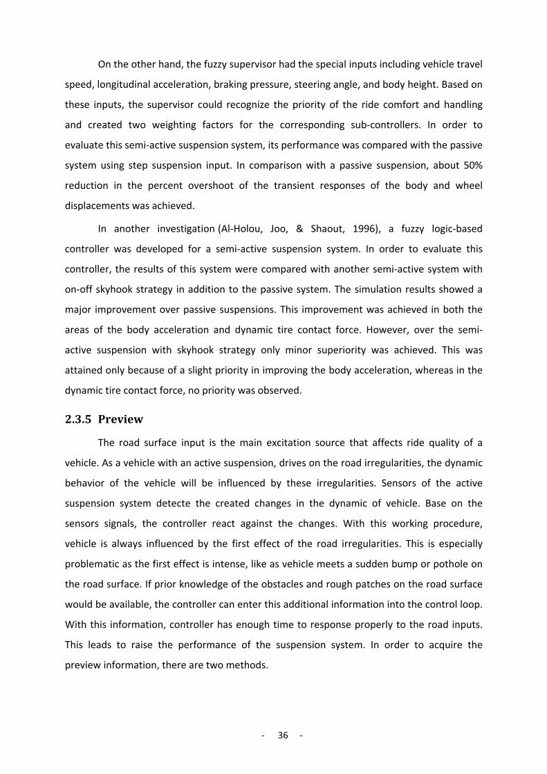
- 36 -

On the other hand, the fuzzy supervisor had the special inputs including vehicle travel

speed, longitudinal acceleration, braking pressure, steering angle, and body height. Based on

these inputs, the supervisor could recognize the priority of the ride comfort and handling

and created two weighting factors for the corresponding sub-controllers. In order to

evaluate this semi-active suspension system, its performance was compared with the passive

system using step suspension input. In comparison with a passive suspension, about 50%

reduction in the percent overshoot of the transient responses of the body and wheel

displacements was achieved.

In another investigation (Al-Holou, Joo, & Shaout, 1996), a fuzzy logic-based

controller was developed for a semi-active suspension system. In order to evaluate this

controller, the results of this system were compared with another semi-active system with

on-off skyhook strategy in addition to the passive system. The simulation results showed a

major improvement over passive suspensions. This improvement was achieved in both the

areas of the body acceleration and dynamic tire contact force. However, over the semi-

active suspension with skyhook strategy only minor superiority was achieved. This was

attained only because of a slight priority in improving the body acceleration, whereas in the

dynamic tire contact force, no priority was observed.

2.3.5 Preview

The road surface input is the main excitation source that affects ride quality of a

vehicle. As a vehicle with an active suspension, drives on the road irregularities, the dynamic

behavior of the vehicle will be influenced by these irregularities. Sensors of the active

suspension system detecte the created changes in the dynamic of vehicle. Base on the

sensors signals, the controller react against the changes. With this working procedure,

vehicle is always influenced by the first effect of the road irregularities. This is especially

problematic as the first effect is intense, like as vehicle meets a sudden bump or pothole on

the road surface. If prior knowledge of the obstacles and rough patches on the road surface

would be available, the controller can enter this additional information into the control loop.

With this information, controller has enough time to response properly to the road inputs.

This leads to raise the performance of the suspension system. In order to acquire the

preview information, there are two methods.

- 37 -

In the first method, the preview sensors are used for collecting the road profile ahead

of vehicles (Fig. 2-14). This sensory information can be used for both the front and rear

suspensions of the vehicles. For that reason, this system has high potential in improving the

performance of vehicle suspensions. However, it needs an advanced sensory set-up and

complex algorithm system in order to derive the road profile from the sensory information

(Baillie, 1999). Different kinds of sensors can be used for this system such as optical,

ultrasonic, and radar technology. In this method, the derivation of the road profile from the

sensory information is the main challenge of the system, and it is often executed with errors.

For example, a pothole filled with water may not be distinguished from the road surface and

cardboard box may not be distinguished from a piece of stone.

Figure 2-14 Preview sensor for active suspension (Donahue, 1998).

Theoretical investigations about this kind of preview control have considered

significant potential profits for these systems, such as the investigation of (Soliman & Crolla,

1996). In spite of this, the experimental investigations have reported some practical

difficulties in achieving these benefits. For example, in the practicable investigation of

(Langlois, Anderson, & Hanna, 1991), an ultrasonic height sensor was used as a look-ahead

preview sensor for an off-road military vehicle, which was equipped with an active

suspension. After testing the vehicle over a rounded bump with 50mm height, the results

showed that the preview control system provided a reduction of 15 % in the RMS

acceleration of the body in comparison with a passive suspension, whereas this system could

offer only 4 % improvement over the active system without preview.

In the second type of preview control systems by measuring the dynamic variables at

the front axle, the road profile under the rear wheel is predicted. The moment that the

roughness reaches to the front wheel can be calculated based on the vehicle speed and

- 38 -

wheelbase. For that reason, this method is called wheelbase preview control. As an

advantage of this system, they do not need to the complex sensory system in the front of the

vehicle. However, in this system, the preview information is only available for the rear

suspension. The investigations about wheelbase preview control have considered grate

potential benefits for this system. For example, in the research work of (Crolla & Abdel-Hady,

1991), the capability of the wheelbase preview system was evaluated by applying it to the

rear semi-active suspension of a vehicle. Based on the results of this investigation, it was

concluded that semi-active systems with preview control strategy have the potential to

achieve a performance over fully active systems.

The research work of (Hansson P. , 1996) is a rare research work in the theme of

active suspensions for fully suspension agricultural tractors. In this research work, a preview

control approach was used for the rear adaptive suspension of a tractor in order to modify

its performance. The primary adaptive suspension of this tractor was not enough fast to deal

with sudden changes in ground roughness, such as potholes. Especially, sudden roughness

on a smooth surface produced a high level of vibration, because on the smooth surface, the

dampers were normally set on the high damping mode by the controller. As the sudden

rougher area reached, the adaptive control was unable to create fast major change in the

damping gain. In this condition, result might be a suspension over-travel, inducing extreme

vibration levels at the driver.

Hansson found that the solution of this problem was to use a preview control system

in order to recognize the sudden road roughness previously. Since the first kind of preview

control with the look-ahead preview sensor was considered too complicated and expensive

for a tractor, the wheelbase preview-control system was chosen. In this system, the

accelerations at the front axle was measured and filtered in order to pre-estimate the

ground roughness under the rear wheel. Using this preview information, the damping

controller was able to determine the optimal damping degree so that, the rear suspension

could use the available travel space in an optimal way. In this way, rear suspension was able

to react effectively to the sudden road inputs.

In summary, employing the preview controls in advanced suspensions provides

encouraging results in improving their performance. However, the technical difficulties are

considered in the practicable application of these systems, particularly about the look-ahead

preview sensors.

- 39 -

2.3.6 On-Off Damping

In a semi-active suspension, dampers are able to generate force only in the opposite

direction of the suspension, and the control strategy includes always a switching law in order

to turn the damper off, as the damping force is in the inverse direction. Because of this

switching, the damping forces are discontinuous in these systems. This issue leads to create

rapid changes in the vehicle body accelerations and consequently, increase the problem of

the jerk and noise. This phenomenon affects negatively its ride quality and handling. This

issue has been also addressed in some research works such as (Karnopp, Crosby, & Harwood,

1974) and (Hauck, 2001). In order to regulate this problem, the difference between

maximum and minimum value of the damping forces should be reduced. The formulation of

the skyhook control strategy was presented before in section 2.3.1. By limiting the values of

the damping coefficients, the formulation of the control strategy can be modified as follows:

)(0)(0)()( max2min

122min

1221222

ccczzzczzzzzzc

c s <<

<′−′′≥′−′′′−′′

= 2-10

As seen, in the “off” mode, a minimum value for damping coefficient is defined instead of

the zero value. In addition, the lowest and highest values of the “on” mode are also limited.

Looking at equation 2-10 as a typical formulation of a continuous semi-active

suspension, it can be realized that a continuous controllable damper is needed in order to

perform a continuous semi-active system. In addition, in order to perform this system, both

the absolute and relative velocities of the suspension must be measured, because the

damping coefficient of the continuous damper is calculated based on these velocities.

However, these conditions can be changed totally with a simple change in the control

strategy.

By looking again at the semi-active strategy, it can be found that this approach works

in this principle that as the damping force is useful for the damping of vibrations, the damper

coefficient is increased to the specific values. Alternatively, as damping force is in the wrong

direction, the damper is turned off to a minimum value for its coefficient. Now, if for the

“on” mode of the damper similar to the “off” mode, just one coefficient would be

considered the major simplification would be achieved. This new strategy is called “on-off

damping” approach and can be defined mathematically as:

- 40 -

<′−′′≥′−′′

=0)(0)(

122

1222 zzzc

zzzcc

statelow

statehigh 2-11

The modes of “off” damping and “on” damping are called respectively as “low state”

and “high state”, referring to the low and high levels of the damping in system. The switching

law of this formulation is based on the skyhook approach, and because of this, it can be

called “on-off skyhook damping” control strategy. However, the switching law can be

defined differently based on the different on-off damping strategies.

On-off damping strategy provides major simplification in the application of a semi-

active system namely in the actuator, sensors, and controller components of the system. In

these systems unlike the continuous systems that need continuous controllable dampers,

just dampers with two levels of damping are necessary. On the other hand, the formulation

of this system implies that the measures of the relative velocity and absolute velocity are

needed in a continuous strategy, whereas just the signs of these velocities are necessary in

on-off strategy.

These simplifications are considered as the main advantage of this strategy in

comparison with the continuous method. These systems can be considered as proper option

for the semi-active suspensions used for agricultural tractors. A new system for these

vehicles, which work under severe operating conditions, should have a relative simple and

robust construction in addition to the good performance. In this research work, this was

considered also as the motivation of choosing on-off skyhook as the proper control strategy

for the semi-active suspension of agricultural tractors.

However, the probable weaknesses of this system should be studied as before to

ensure that this strategy provides a good efficiency for the system. Because of the

phenomenon of the discontinuous damping force in the on-off strategy, the most

challenging problem is the increasing jerk and noise in the system. “Miller” and “Nobles” in

their investigation (Nobles & Miller, 1985) tried to find a solution in order to overcome against

this problem in semi-active suspensions. They found finally that the method of creating a

limitation for the damping force range was completely effective in both continuous and on-

off semi-active suspensions. As a result, in order to overcome against this problem in on-off

strategy, a more limited range for the high and low level of damping should be defined as:

𝒄𝒄𝒉𝒉𝒉𝒉𝒉𝒉𝒉𝒉 𝒔𝒔𝒔𝒔𝒔𝒔𝒔𝒔𝒔𝒔 < 𝒄𝒄𝒎𝒎𝒔𝒔𝒎𝒎 , 𝒄𝒄𝒎𝒎𝒉𝒉𝒎𝒎 < 𝒄𝒄𝒍𝒍𝒍𝒍𝒍𝒍 𝒔𝒔𝒔𝒔𝒔𝒔𝒔𝒔𝒔𝒔 2-12

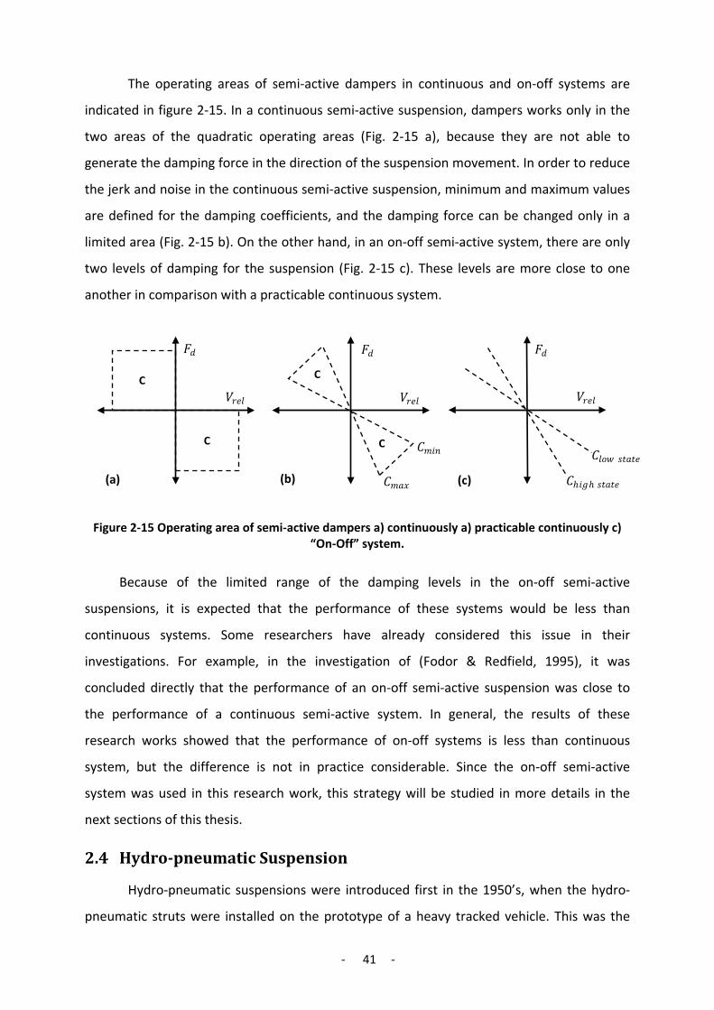
- 41 -

The operating areas of semi-active dampers in continuous and on-off systems are

indicated in figure 2-15. In a continuous semi-active suspension, dampers works only in the

two areas of the quadratic operating areas (Fig. 2-15 a), because they are not able to

generate the damping force in the direction of the suspension movement. In order to reduce

the jerk and noise in the continuous semi-active suspension, minimum and maximum values

are defined for the damping coefficients, and the damping force can be changed only in a

limited area (Fig. 2-15 b). On the other hand, in an on-off semi-active system, there are only

two levels of damping for the suspension (Fig. 2-15 c). These levels are more close to one

another in comparison with a practicable continuous system.

Figure 2-15 Operating area of semi-active dampers a) continuously a) practicable continuously c) “On-Off” system.

Because of the limited range of the damping levels in the on-off semi-active

suspensions, it is expected that the performance of these systems would be less than

continuous systems. Some researchers have already considered this issue in their

investigations. For example, in the investigation of (Fodor & Redfield, 1995), it was

concluded directly that the performance of an on-off semi-active suspension was close to

the performance of a continuous semi-active system. In general, the results of these

research works showed that the performance of on-off systems is less than continuous

system, but the difference is not in practice considerable. Since the on-off semi-active

system was used in this research work, this strategy will be studied in more details in the

next sections of this thesis.

2.4 Hydro-pneumatic Suspension

Hydro-pneumatic suspensions were introduced first in the 1950’s, when the hydro-

pneumatic struts were installed on the prototype of a heavy tracked vehicle. This was the

𝐹𝐹𝑟𝑟

𝑉𝑉𝑟𝑟𝑒𝑒𝑓𝑓

𝐶𝐶ℎ𝑝𝑝𝐾𝐾ℎ 𝑁𝑁𝑡𝑡𝑟𝑟𝑡𝑡𝑒𝑒

𝐶𝐶𝑓𝑓𝑜𝑜𝑙𝑙 𝑁𝑁𝑡𝑡𝑟𝑟𝑡𝑡𝑒𝑒

(c)

𝐹𝐹𝑟𝑟

𝑉𝑉𝑟𝑟𝑒𝑒𝑓𝑓

𝐶𝐶𝑚𝑚𝑟𝑟𝑥𝑥

𝐶𝐶𝑚𝑚𝑝𝑝𝑛𝑛

C

C

(b) (a)

𝐹𝐹𝑟𝑟

𝑉𝑉𝑟𝑟𝑒𝑒𝑓𝑓 C

C

- 42 -

result of an investigation with the purpose of using compressible fluids in suspension

systems, conducted by two German companies (Hilmes, 1982). After that, hydro-pneumatic

suspension was used for automobiles by Citroen Company as the first time in the mid-

1950’s. In this way, the superior capability of this system for the automobiles was proved as

well as in heavy vehicles. However, in the beginning, there were some shortages such as the

problems of improper sealing and heat influence of the system. During the next years, by

using new hydraulic technology, the problem of sealing was solved, and the temperature

influence was removed by employing the load leveling control system (Giliomee, 2003).

The principle of a hydro-pneumatic suspension is illustrated in figure 2-16. A

hydraulic cylinder is placed between the chassis and wheel of the vehicle instead of the

spring and damper in conventional suspensions. This cylinder has a hydraulic connection to

an accumulator through a throttle. As the cylinder is compressed, oil is forced to the

accumulator through the throttle. This condenses the gas inside the accumulator and

produces a pressure in the accumulator that appears as the stiffness force on the cylinder.

On the other hand, the pressure drop on the throttle creates the damping force on the

cylinder. More detail of this system will present in chapter 2.

Figure 2-16 Configuration of a hydro-pneumatic suspension system.

Since the stiffness property of a hydro-pneumatic suspension is created based on the

gas compression, unlike steel springs, the stiffness is not linear, and it rises progressively

with increase in the suspension displacement. This characteristic decreases the influence of

the load variation on the natural frequencies of the vehicle body. In addition, the overload

capability of this suspension type is improved, because the stiffness of the suspension rises

largely at the end of its strike.

- 43 -

One important feature of hydro-pneumatic suspensions is the controllability of this

system that can be equipped with different types of control systems. Figure 2-17 illustrate

the methods of converting this system to an active suspension. In figure 2-17 (a), a

controllable throttle valve is used between the cylinder and accumulator in order to control

the damping level of the suspension. This mechanism can be used as the actuation system of

semi-active or adaptive suspensions. On the other hand, by applying the pressurized oil from

a hydraulic pump to the hydro-pneumatic suspension, this system can be used as an

actuation system for fully active or for a load leveling suspension systems (Fig 2-17, b).

Figure 2-17 Capability of hydro-pneumatic suspensions in converting to different types of active system.

In hydro-pneumatic suspensions, variable stiffness can be also provided in addition to

the variable damping mechanism. This ability is created by changing the primary pressure of

the gas in the accumulator, which can be performed by pressurizing oil to the cylinder or

pulling oil out from it. In order to create major changes in the level of stiffness, extra

accumulators can be used. These accumulators are connected to the cylinder via the on/off

valves. Vehicle load leveling system is an application of the variable stiffness. In addition, the

variable stiffness can be used in order to create an adaptive suspension system like in the

research work of (Abd El-Tawwab, 1997). In this investigation, in addition to use a throttle

valve for creating a controllable damping system, an on/off valve with an extra accumulator

was used in order to create a controllable stiffness mechanism (Fig. 2-18).

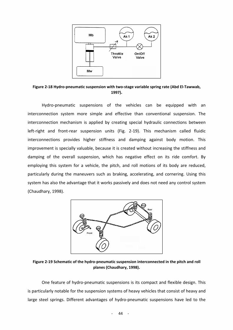
- 44 -

Figure 2-18 Hydro-pneumatic suspension with two-stage variable spring rate (Abd El-Tawwab, 1997).

Hydro-pneumatic suspensions of the vehicles can be equipped with an

interconnection system more simple and effective than conventional suspension. The

interconnection mechanism is applied by creating special hydraulic connections between

left-right and front-rear suspension units (Fig. 2-19). This mechanism called fluidic

interconnections provides higher stiffness and damping against body motion. This

improvement is specially valuable, because it is created without increasing the stiffness and

damping of the overall suspension, which has negative effect on its ride comfort. By

employing this system for a vehicle, the pitch, and roll motions of its body are reduced,

particularly during the maneuvers such as braking, accelerating, and cornering. Using this

system has also the advantage that it works passively and does not need any control system

(Chaudhary, 1998).

Figure 2-19 Schematic of the hydro-pneumatic suspension interconnected in the pitch and roll planes (Chaudhary, 1998).

One feature of hydro-pneumatic suspensions is its compact and flexible design. This

is particularly notable for the suspension systems of heavy vehicles that consist of heavy and

large steel springs. Different advantages of hydro-pneumatic suspensions have led to the

- 45 -

frequent use of this system for different vehicles. For example, these suspensions are

employed widely for the agricultural tractors, because of their compact and flexible design

and also their control ability. In these vehicles, the auto leveling system, which is needed

especially because of their wide range of loads, can be applied simply to the hydro-

pneumatic suspension. In addition, for station work or extreme working condition of

tractors, suspension blockage mode is necessary. This mechanism can also be added simply

to a hydro-pneumatic suspension by using hydraulic valves, so as to block the oil in the

cylinders (Fig. 2-20).

Figure 2-20 Suspension blockage mode by using the valves between the accumulators and cylinder (Bauer, 2007).

In this investigation, a semi-active control system was applied to the hydro-pneumatic

suspension of the rear axle of an agricultural tractor. For that reason, in the next sections of

this thesis, more theory and practical details will be presented about the hydro-pneumatic

suspension systems.

2.5 Suspension System for Tractors

In the previous sections, the suspension system of vehicles was studied in general.

Now, in this part, employment of the suspension systems for agricultural tractors is

considered. The early agricultural tractors had no suspension systems, and different types of

suspension systems were employed in them gradually with time. The primary systems were

seat suspensions, which were used with the aim of improving ride comfort of tractors. Along

with the development in tractors technology, chassis suspensions were also used for these

vehicles.

These systems were able to improve the handling of tractors besides the ride comfort

of them. This provided more safety and stability for tractors, and their travel speed was

increased. In this part of thesis, suspension systems used for agricultural tractors are studied.

- 46 -

This begins with characteristics of tires, and suspensions of seat and cabin. Then, the chassis

suspension systems of tractors including front axle and full suspension are explained. Finally,

as the summary of this part, the general characteristics of these systems are presented.

2.5.1 Suspension Characteristics of Tires

When in the early 30th, the pneumatic tires were used first time for agricultural

tractors, ride comfort and handling were improved, and the travel speed of tractors was

increased until 20 km/h (Hoppe-01, 2004). Tires are the first elastic elements between a

vehicle and the ground surface. For that reason, the suspension properties of the tires have

an important role in the dynamic behavior of tractors, particularly for tractors having no

other suspension systems.

The suspension characteristic of a tire can be demonstrated by a simple model, which

is constructed of a spring and a damper in parallel (Fig. 2-21). Based on this model, figure 2-

22 presents the measured stiffness and damping characteristic of a typical tire for

agricultural tractors. As shown, the stiffness and damping coefficients of the tire are

correspondingly too high and too low than typical suspension characteristic needed for a

tractor. Therefore, tires are not able to work lonely as a proper suspension system, because

high stiffness of tires is equal to a very hard suspension that is unable to provide good ride

comfort. On the other hand, with very low damping capacity of tires, they are not able to

provide effective control on vibrations.

Figure 2-21 Single point contact modeling of tires.

In addition to the improper value of stiffness and damping coefficient of tires, these

characteristic are not constant and depend on the inflation pressure and speed of tires. All

these factors cause a poor dynamic behavior for the conventional tractors that have no

primary suspension, and the tires are the only elastic element working as a suspension for

them. This is particularly considerable in the heave and pitch vibration of the tractors in the

- 47 -

high travel speed (Von Holst, 2000). With the raise in the travel speed of them, the road

excitations are increased, and in the same time, the damping coefficient of the tires is

reduced. The speed range of 50 - 60 km/h is reported as the critical driving condition of

conventional tractors on the standard roads (Vessonen & Järviluoma, 2001). In the worst

case, because of the resonance phenomenon, the vibration amplitude can be increased until

15 times and reach to the limit where the wheels lose their contact to the road surface. This

may reduce largely the steer ability of the tractors and creates an unsafe mode for them.

Figure 2-22 Influence of the travel speed on tire suspension characteristics a) tire damping rate b) tire stiffness coefficient (Von Holst, 2000).

As whole, in the lacking of a primary suspension, the insufficient suspension property of

tires creates these consequences for conventional tractors (Von Holst, 2000):

- Low handling, which causes low driving safety and low travel speed.

- 48 -

- Poor ride comfort, which decreases driver efficiency and can harm his healthy.

- Pavement damage, which is particularly problematical for the public asphalt

roadways used for the transportation.

As mentioned, the inflation pressure of a tire has significant influence on its

characteristics. Based on this fact, some research works have been conducted with the

theme of “Central Tire Inflation Systems” (CTIS). In these investigations, it was intended to

improve dynamic behavior and traction power of the tractors via an optimal control on the

tires inflation pressure. These investigations were confirmed that a significant improvement

in ride comfort of tractors could be achieved as the inflation pressure was optimally

controlled (Ulrich, 1983).

In addition, in the research work of (Kaczmarek, 1984) it was shown that the handling

capability of a vehicle could be improved also by this system. This improvement could be

created by modifying the natural frequency of the vehicle via an optimal control of the tires

stiffness. However, in spite of these achievements by the CTIS systems, the tires are not still

able to provide a good dynamic behavior, and this implies that the suspension systems are

totally needed for the agricultural tractors. The different suspension systems that are

employed in the agricultural tractors will be explained in the following sections.

2.5.2 Seat Suspension

Problem of the vibration transmitted to the operators of agricultural tractors has

been widely discussed over the last 40 years (Marsili, Ragni, Santoro, & Servadio,

2002).Operators of conventional agricultural tractors are exposed to a high level of

vibrations during typical farm operations (Scarlett, Price, & Stayner, 2007). On the other

hand, they work normally for a long time on the tractors particularly during intensive

working seasons. The high level of vibrations experienced by an operator is harmful for his

health and creates an early fatigue. This consequence decreases the efficiency of operators.

In order to overcome against this problem and decrease the vibration transmitted to

the operators, employment of suspension systems has been considered. The first system

used for this purpose is the suspension for the seat of the operator. This system is placed

directly between the driver seat and tractor body, and it affects directly driver comfort and

reduces the vibration experienced by him. Seat suspensions are uncomplicated, inexpensive

and have a robust construction. For these reasons, they are employed now for nearly the

- 49 -

whole modern agricultural tractors. A suspension seat is made of typically a foam cushion

suspended on a parallel spring and damper set. Type of suspension systems may be

mechanical, pneumatic, hydraulic, hydro-pneumatic, or a combination of these systems.

In order to improve the performance of seat suspensions, active suspension

technology have been employed. For example in the investigation of (Hauck, 2001), a semi-

active suspension with a MR damper as the actuator was employed in the seat suspension of

the agricultural tractors. This system was evaluated by both computer simulation and

experimental testing. In the experimental part, the tests were performed by use of a

suspension test rig. According to the simulation tests, a reduction until 22 % was achieved in

seat RMS acceleration in comparison with passive damping. However, in the experimental

tests, this improvement was fallen into 9 % improvement.

Considering the low total mass of a seat and driver, using fully active systems for seat

suspensions causes no high extra consumption of energy. Therefore, these systems have

been also considered as practical systems in order to improve the performance of the seat

suspensions. In this theme, (Stein & Ballo, 1991) conducted a research project with the

purpose of measuring the required energy for an active seat suspension. For this purpose,

they considered a low bandwidth fully active seat suspension, which used a hydraulic force

actuator combining with a passive spring-damper system. As a result, this system could

provide full vibration isolation until 3 Hz by consuming the maximum power of 2.2 kW.

The application of active suspension systems for the seat suspension has been

considered by most of the well known agricultural tractor companies with the aim of offering

a high level of ride comfort for the operators of tractors. Figure 2-23 shows a modern seat

from John Deere with an active seat technology. This seat technology uses a full active

hydro-pneumatic suspension. This system receiving 200 Hz sensory inputs is able to reduce

the excessive vertical movement of the seat. This provides more comfortable ride, and

consequently, the operator can travel faster in hard field conditions.

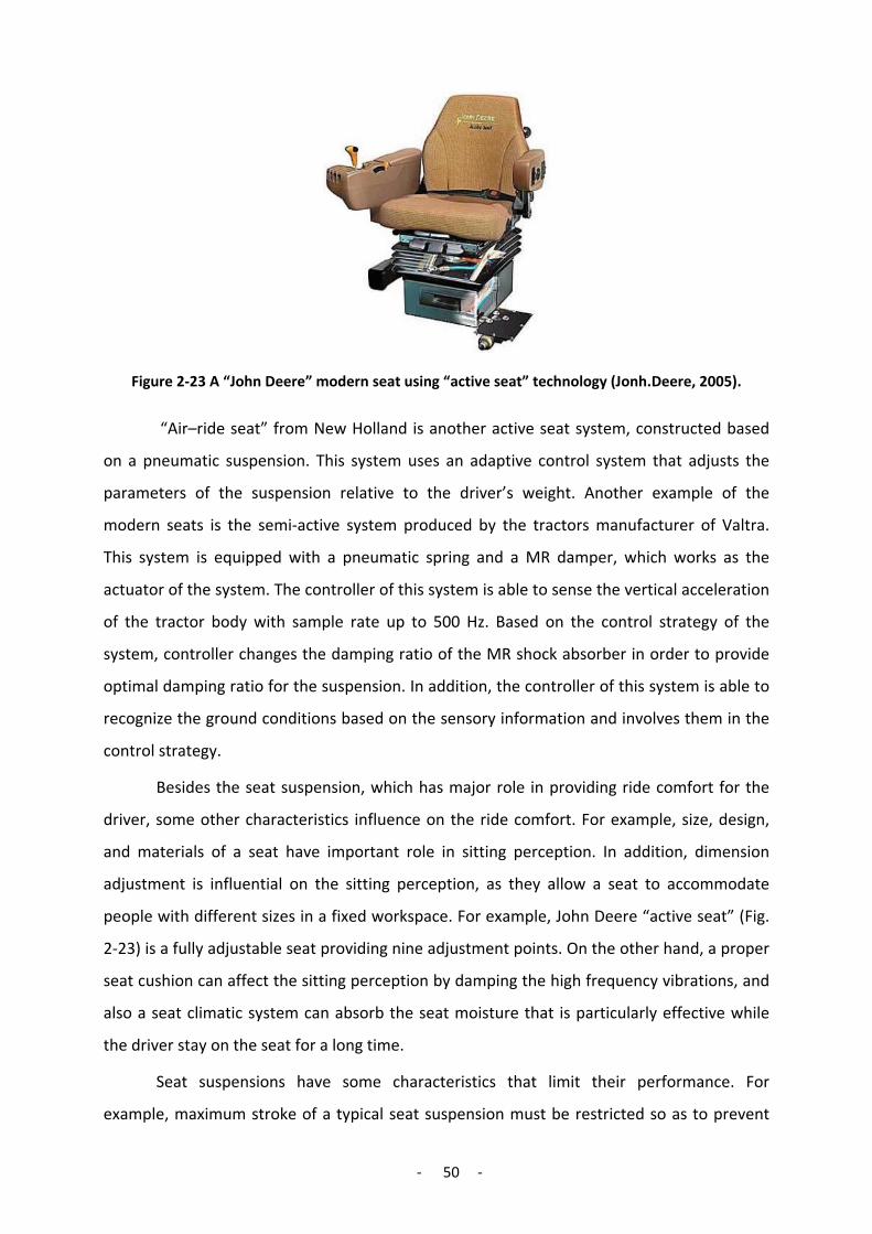
- 50 -

Figure 2-23 A “John Deere” modern seat using “active seat” technology (Jonh.Deere, 2005).

“Air–ride seat” from New Holland is another active seat system, constructed based

on a pneumatic suspension. This system uses an adaptive control system that adjusts the

parameters of the suspension relative to the driver’s weight. Another example of the

modern seats is the semi-active system produced by the tractors manufacturer of Valtra.

This system is equipped with a pneumatic spring and a MR damper, which works as the

actuator of the system. The controller of this system is able to sense the vertical acceleration

of the tractor body with sample rate up to 500 Hz. Based on the control strategy of the

system, controller changes the damping ratio of the MR shock absorber in order to provide

optimal damping ratio for the suspension. In addition, the controller of this system is able to

recognize the ground conditions based on the sensory information and involves them in the

control strategy.

Besides the seat suspension, which has major role in providing ride comfort for the

driver, some other characteristics influence on the ride comfort. For example, size, design,

and materials of a seat have important role in sitting perception. In addition, dimension

adjustment is influential on the sitting perception, as they allow a seat to accommodate

people with different sizes in a fixed workspace. For example, John Deere “active seat” (Fig.

2-23) is a fully adjustable seat providing nine adjustment points. On the other hand, a proper

seat cushion can affect the sitting perception by damping the high frequency vibrations, and

also a seat climatic system can absorb the seat moisture that is particularly effective while

the driver stay on the seat for a long time.

Seat suspensions have some characteristics that limit their performance. For

example, maximum stroke of a typical seat suspension must be restricted so as to prevent

- 51 -

the suspension from excessive displacement between the driver and the vehicle control

equipments (Boileau & Rakheja, 1990). In order to restrict the travel of the seat suspension,

rubber bump-stops are often used. However, contact with the bump stops can lead to a

higher level of vibrations on the seat over than the vehicle floor (Gunston, 2000). In order to

avoid this experience, a stiffer spring should be used. However, this increases the resonant

frequency of the seat closely to the resonant frequency of the vehicle. This leads to a higher

transmission of the vibrations to the seat, and it is the main restriction of the seat

suspensions.

On the other hand, whereas seat suspension is able to reduce effectively the vertical

vibration of the tractor body, it is very difficult to achieve effective vibration isolation by seat

suspension in horizontal and rotational directions. These vibrations are particularly

important, because they have high amplitude on the body of agricultural tractors and have a

significant influence on ride quality (Suggs & Huang, 1969). In order to remove these weak

points and achieve better performance, besides the seat suspension, the other types of

suspension systems such as cabin and chassis suspension should be used.

2.5.3 Cabin Suspension

In modern agricultural tractors, a cabin is used in order to isolate the driver from the

outside, and it protects the driver from the annoying environmental conditions, dust, and

noise. Using a suspension system for the cabin, driver place could be isolated from the

tractor vibrations as well.

A cabin suspension can offer more benefits than a seat suspension and provide

better ride comfort for the driver. These advantages can be stated as follow:

• It provides vibration isolation for both the driver and the control equipments beside

him. In this way, the problem of the relative movement between the driver and the

control equipments is eliminated (Hansson P. , 1995).

• Cabin suspension decreases the structurally transmitted noise to the drivers.

• Cabin suspension is able to isolate the driver from the rotational vibrations of the

tractor body in addition to the vertical vibrations.

• Since the mass of a cabin is greater than a seat, the natural frequency of cabins is

lower than the one of seat suspensions. This leads to provide better vibration

isolation (Von Holst, 2000).

- 52 -

• Because of the greater mass of a cabin, the variation in the drivers’ weight has less

influence on the performance of the cabin suspension.

The manufactured cabin suspensions of the agricultural tractors can be categorized in

two groups of semi suspended and fully suspended. In the first group, the rear side of the

cabin is connected to the chassis by means of two suspension units in its corners. In spite of

this, the front side is connected to the tractor chassis without suspension and only via a

joint-type link. This type is often used for the tractors with front axle suspension. In this

system, body vibrations appear on the cabin as pitch rotational movement, and response of

this system to the roll movement of the tractor body is very limited.

An example of this system is the cabin suspension of Deutz Agrotron tractors. The

suspension units used for this system are pneumatic-type (Fig. 2-24). This suspension is

controlled by an adaptive control system that adjusts the stiffness of suspension relatively to

the load of the cabin. Benefiting this control system, the used suspension strike is just 40

mm.

Figure 2-24 “Deutz” semi suspended cabin using pneumatic suspension units (Deutz, 2006).

Another type of the cabin suspensions is the fully suspended cabin, which is

constructed by four suspension units in the corners of the cabin. With this construction, this

system is capable to damp all six degrees of vibrations of the dimension and rotational

directions (Goehlich, 1984). This type of cabin suspensions have already used by tractor

companies of “Class” and “Renault” for their productions.

The cabin suspension of the agricultural tractors has been already the theme of some

research works such as (Kauss & Weigelt, 1980) and (Hilton & Moran, 1975). All these

investigations confirmed the capability of the cabin suspensions in providing good ride

comfort, especially as it was compared with seat suspensions. However, the cabin

- 53 -

suspension still suffers from the same problem of high natural frequencies due to the limited

travel space. These resonant frequencies are close to those of the tractor body and causes

high vibration transmitting.

In order to improve the performance of the cabin suspensions, the idea of active

suspensions can be considered. In this theme, there are some research projects, such as the

work of (Hansson P. , 1995). In this investigation, a combination of the adaptive and fully

active suspension was used for a cabin suspension intended primarily for the agricultural

tractors. In this system, based on a linear optimal control technique, the feedback gains of

the controller was varied iteratively so that the controller always strived to make the

optimum use of the available travel space. The efficiency of this system was evaluated in the

terms of the vibration isolation and power consumption. Based on the positive results and

low power consumption, the active cabin suspensions are recommended for the practicable

application. In addition to these investigations, the active cabin suspension has been already

employed by tractor companies such as Fendt and Deutz for their productions.

Cabin suspensions have no considerable influence on the dynamic behavior and

handling capability of the tractors, because the mass of the cabins (300-600 kg) is very low in

comparison with the total mass of the tractors. In this condition, the cab suspension can

create only a small reduction in the natural frequency of the tractors. However, in the

investigation of (Von Holst, 2000), it was concluded that the handling capability of the rear

axle in a conventional tractor can be affected significantly by the cab suspension, because in

these tractors, the cabin places on the rear axle, and the handling effect of the cabin

suspensions is focused on this axle.

As conclusion, a cabin suspension provides good ride comfort but have no significant

influence on the handling of the tractors. In order to provide both good ride comfort and

good handling, in addition to the secondary suspensions, the primary suspensions is needed.

The secondary suspension is referred here to the cabin and seat suspensions, and the

primary suspension is referred to the chassis suspensions, which will be described in the

following sections.

2.5.4 Hitch Suspension

During transportation, tractors are often mounted with heavy implements. These

heavy implements change largely the mass characteristics of the tractors, and influence

- 54 -

mainly the dynamic behavior of the tractors. On the other hand, tractors have typically no

axle suspensions, particularly no one for the rear axle. Without the primary suspension, the

tires are the only elastic elements that affect the handling of the tractors, whereas the tires

have no required suspension properties. Under these conditions, the dynamic behavior of

the tractor becomes worse under the influence of the attached implements, particularly the

bounce and pitch movement of the tractor are increased. This situation causes a fall in the

control ability of the tractor, which especially during high-speed transports leads to unsafe

modes.

In order to reduce the effect of the mounted implements on the tractors and in order

to control their vibration, a suspension system can be used in the connection between them

and the tractors. Since the implements are normally mounted on a tractor via the three-

point hitch, this suspension is applied to this mechanism and called “hitch suspension”.

Figure 2-25 illustrates such a system that employs a hydro-pneumatic suspension in damping

the pitch vibration of the implement. As shown, a hydraulic actuator is used instead of the

upper link in this system. This actuator is connected to a hydraulic accumulator through a

throttle valve and works as a hydro-pneumatic suspension.

Figure 2-25 A hydro-pneumatic shock absorber system applied to the tractor three-point hitch (Goehlich, 1984).

In order to improve the performance of hitch suspensions, the active suspensions can

be used. All types of active suspension such as fully active, semi-active, and adaptive control

could be applied to a hitch suspension. Since the primary hitch suspensions are usually

hydro-pneumatic, the actuation system of the active systems can be performed typically by

using an adjustable throttle between the cylinder and accumulator for semi-active system

and energizing oil to the cylinder for fully active system. According to the natural frequency

Valve

Hydraulic accumulator (shock absorber)

Implement

Hydraulic actuator (upper link)

- 55 -

of a hitch suspension, the control system of these active suspensions works with the

bandwidth of less than 3 Hz (Hoppe-01, 2004).

There are some research works in this area like the research work of (Hansen &

Andersen, 2003). In this investigation, in order to damp the pitch vibration of the tractor

body, a fully active hitch suspension was used for controlling the vibrations of the mounted

implements. Figure 2-26 shows the components of this system. A plough used as the

implement of the system was hung from the rear end of the tractor via a three-point hitch

linkage. This linkage was typically actuated by two so-called hitch hydraulic cylinders, which

were used as the actuator of the active hitch suspension. It was intended that for damping

the pitch movement of the tractor body, the actuators were controlled to move the

implement appropriately to the vibration of the tractor body in order to neutralize it. For

controlling the cylinders forces, the directional solenoid-valves were used to control the

connection of the cylinders to the hydraulic pump and the tank.

Hansen considered two different control strategies for the system. The first one was

based on measuring the cylinders oil pressure, and the second one was based on measuring

the pitch angle of the tractor body. The first control strategy strived to maintain the

derivative of the pressure signal substantially constant at the value of zero, and the second

control strategy strives to keep the derivative of the pitch angle at the value of zero. After

evaluation of the system, it was concluded that both the strategies created significant

improvement in performance of the hitch suspension in comparison with the non-controlled

system.

Figure 2-26 Full active vibration control system used for the tractor three-point hitch suspension (Hansson P. , 1995).

The influence of the hitch suspension on the dynamic behavior of tractors is

dependent on the quantity of the mass and moment of inertia of the mounted implement.

- 56 -

For the heavy implements, experimental and analytical studies have shown that the rear

hitch suspension modifies the vibration behavior of the tractors significantly, and in this way

first, they have a great positive influence on the steering and drive safety of the tractors, and

secondly, they improve the ride comfort of tractors (Ulrich, 1983) & (Von Holst, 2000).

For adding a hitch suspension system to a tractor, the main structure of the typical

three-point hitch can be employed, and in this manner, no constructional change is

necessary, and this suspension can be added to the tractors relative simply with low

expense, whereas they can create large improvement in the vibration behavior of the

tractor. Presently, most of the modern tractors are equipped with this kind of suspension

system.

2.5.5 Front Axle Suspension

During the late 1980’s, four Wheel Drive (4WD) tractors became popular due to the

better traction performance. Using these tractors, the front wheels acquired a new role in

the traction capability of the tractors and also in the steering ability of them. In this

condition, the typical problem of the pitch movement of the tractors was more noticeable,

because it created a load variation on the front tires and caused the problem of bouncing,

particularly during the pulling heavy loads by tractors. This produced a traction variation

effect, called “power hop,” that was not only uncomfortable for the operator, but also

caused a major loss in the traction efficiency of the tractors.

In order to overcome against this problem, the front axle suspension was used for

tractors. This suspension provided a stable contact between the front tires and ground that

leads to a significant improvement in the traction and steering capability of tractors. Because

of this advantage, front axle suspension has become a common option in 4WD tractors now.

In addition, the front wheels are the navigating wheels. They take the major steering and

brake loads of a tractor. Front suspension by keeping front tires in firm contact with the

ground, allows better steering control and brake efficiency. This promotes the handling

capability and increases consequently the travel speed of a tractor. The improvements

created by using front suspensions have been confirmed also in some references such as

(Rhenius, 1983), (Weigelt, 1987) and (Rill, Slag, & Wilks, 1992).

However, influence of the front suspension on ride comfort of tractors is not notable

as much as the influence of this system on the handling of tractors. In the research work of

- 57 -

(Weigelt, 1987) a front suspension was applied to a test-tractor with standard construction

(i.e. typical tractor construction with rear big wheels (Fig 2-27)). The evaluation of the

dynamic behavior of this tractor showed that by using front suspension, the handling of the

tractor was improved significantly. But, the influence of the front suspension on the vertical

acceleration of the seat was not considerable. This occurred, because in standard

constructive tractors, seat position is on top of the rear axle, and the front suspension had

no effect on the bouncing movement of the rear part of tractors body and only reduced the

pitching movement of the tractors.

Figure 2-27 Typical standard and system constructive tractors.

As mentioned, in the standard constructed tractors, using the front suspensions does

not reduce the vertical acceleration of the driver’s seats. In the investigation of (Pickel P. ,

1993), the influence of the seat position on the vertical acceleration was investigated. Figure

2-28 indicates the result of this investigation that is presented as the RMS value of the

vertical acceleration of the seat. This value is presented in respect to the position of the seat

on the tractor body. The examination was performed for the standard and system types of

tractors in the two modes of the suspended front axle and rigid front axle. System tractors

are the tractors that have the same rear and front tire size, and the seat is located in a

position between two axles and standard tractors are the typical tractors with rear big

wheels (Fig. 2-27).

As shown in this graph, the front axle suspension has a minor effect on the vertical

acceleration of the seat, which is located nearly over the rear axle. On the other hand,

position of the seat in a system tractor is between two axles, and the front axle suspension

can reduce the vertical acceleration of the seat considerably. Therefore, when the front

suspensions are employed with the aim of improving the ride comfort, the system tractors

have priority over standard tractors. However, in order to convert a standard tractor to a

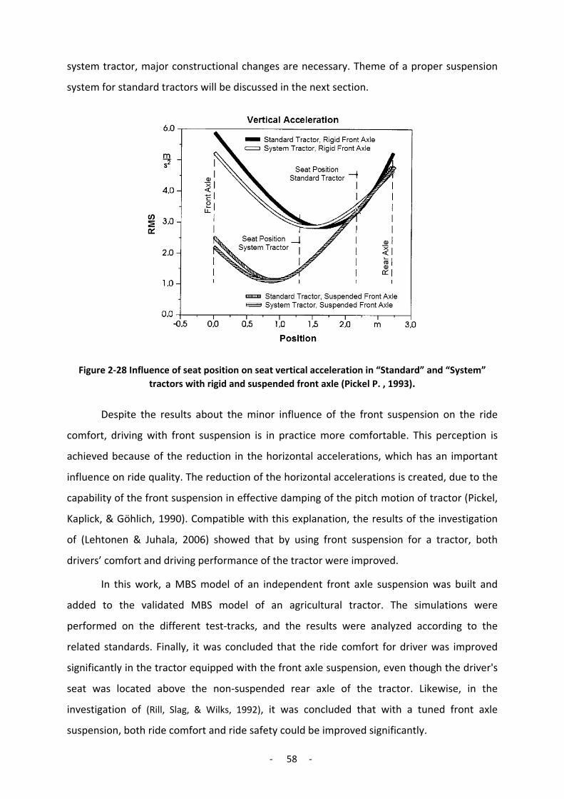
- 58 -

system tractor, major constructional changes are necessary. Theme of a proper suspension

system for standard tractors will be discussed in the next section.

Figure 2-28 Influence of seat position on seat vertical acceleration in “Standard” and “System” tractors with rigid and suspended front axle (Pickel P. , 1993).

Despite the results about the minor influence of the front suspension on the ride

comfort, driving with front suspension is in practice more comfortable. This perception is

achieved because of the reduction in the horizontal accelerations, which has an important

influence on ride quality. The reduction of the horizontal accelerations is created, due to the

capability of the front suspension in effective damping of the pitch motion of tractor (Pickel,

Kaplick, & Göhlich, 1990). Compatible with this explanation, the results of the investigation

of (Lehtonen & Juhala, 2006) showed that by using front suspension for a tractor, both

drivers’ comfort and driving performance of the tractor were improved.

In this work, a MBS model of an independent front axle suspension was built and

added to the validated MBS model of an agricultural tractor. The simulations were

performed on the different test-tracks, and the results were analyzed according to the

related standards. Finally, it was concluded that the ride comfort for driver was improved

significantly in the tractor equipped with the front axle suspension, even though the driver's

seat was located above the non-suspended rear axle of the tractor. Likewise, in the

investigation of (Rill, Slag, & Wilks, 1992), it was concluded that with a tuned front axle

suspension, both ride comfort and ride safety could be improved significantly.

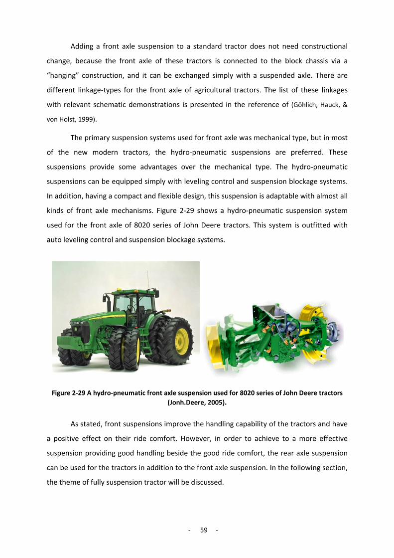
- 59 -

Adding a front axle suspension to a standard tractor does not need constructional

change, because the front axle of these tractors is connected to the block chassis via a

“hanging” construction, and it can be exchanged simply with a suspended axle. There are

different linkage-types for the front axle of agricultural tractors. The list of these linkages

with relevant schematic demonstrations is presented in the reference of (Göhlich, Hauck, &

von Holst, 1999).

The primary suspension systems used for front axle was mechanical type, but in most

of the new modern tractors, the hydro-pneumatic suspensions are preferred. These

suspensions provide some advantages over the mechanical type. The hydro-pneumatic

suspensions can be equipped simply with leveling control and suspension blockage systems.

In addition, having a compact and flexible design, this suspension is adaptable with almost all

kinds of front axle mechanisms. Figure 2-29 shows a hydro-pneumatic suspension system

used for the front axle of 8020 series of John Deere tractors. This system is outfitted with

auto leveling control and suspension blockage systems.

Figure 2-29 A hydro-pneumatic front axle suspension used for 8020 series of John Deere tractors (Jonh.Deere, 2005).

As stated, front suspensions improve the handling capability of the tractors and have

a positive effect on their ride comfort. However, in order to achieve to a more effective

suspension providing good handling beside the good ride comfort, the rear axle suspension

can be used for the tractors in addition to the front axle suspension. In the following section,

the theme of fully suspension tractor will be discussed.

- 60 -

2.5.6 Full Suspension

Higher travel speed is taken into consideration for the modern tractor design,

because road vehicles such as trucks do not fulfill all the necessities of the agricultural

transport-purposes. This led to try for development of high tractor speeds, which are able to

cover the transportation needs of agricultural applications (Goehlich, 1984). As mentioned,

employment of the front suspensions in tractors provided a major benefit regarding to the

high travel speed. However, front axle suspensions can be sufficient just to reach to a limited

maximum speed. In order to achieve a higher speed, the unique approach can be found in

employment of the full suspension in tractors. A full suspension tractor is a tractor equipped

with both rear and front axle suspensions. These tractors can provide improvement on both

driving behavior and ride comfort, promising the possibility for the rise in the driving speed.

Tractors with only front suspensions cannot present a perfect dynamic characteristic.

As mentioned, the influence of the front suspensions on ride comfort of the tractors is not

significant, especially on the vertical vibration of the seat. In addition, this influence depends

on the position of the seat between two axles. About the handling capacity of tractors, front

suspensions have a good efficiency. However, disadvantageously, the front axle suspension

affects negatively the vibration behavior of the unsuspended rear axle, which keeps more

than half of the load of the tractor, because by using front axle, rotation axle of the pitch

body oscillation shifts to the rear axle. This increases the bounce of the rear wheels and

decreases consequently the tires contact to the road surface.

On the other hand, the front suspensions have significant effects only on the pitch

and longitudinal vibration of the tractors, whereas the rear suspension influences the

vibrations in most of the directions, particularly in the important vertical direction (Hansson

P. , 1996). After all, using the rear axle suspension besides the front suspensions can end

these problems by creating an essential contribution in vibration isolation at both the rear

and front axles. In this way, a full suspension system provides both safe driving and good ride

comfort for the tractors. The previous research works also have already illustrated the

superior characteristics of the full suspension tractors (Claar, Sheth, Marley, & Buchele,

1980).

Despite of the advantages of the full suspension tractors, adding the rear suspensions

to the conventional tractors is not as simple as the front suspensions. This is originated from

the typical structure of the conventional or standard tractors, which are about 80 % of the

- 61 -

whole agricultural tractors (Kaplick C. , 1995). These tractors have a similar construction and

called block construction (Fig.2-30). These tractors have a block construction, instead of the

chassis construction. This construction is formed by connecting the three blocks of engine,

transmission, and rear axle unit. Since primary types of these tractors have just rear drive

wheels, in order to achieve optimal traction, at least 60% of their weight stands on the rear

axle, and the rear wheels are selected bigger and heavier than the front wheels.

Figure 2-30 Block construction of “Standard” tractors (Müller, 2001).

In these tractors, front axle is linked to the block via a hanging-type junction and

driver seat is positioned over the rear axle (Fig. 2-30). Adding front axle suspension to this

structure is simply possible and needs no major changes. In the case of the rear axle

suspension, the issue is not simple. In a standard tractor, axle of the rear wheels is fixed

directly to the block of the tractor, and in this way, it is related directly to the transmission.

With this structure, in order to add rear axle suspensions to standard tractors, basic changes

in the construction of these tractors are necessary. The block structure of these tractors is

not just for the rear suspension problematic. Each modification on the main components of

these tractors, such as engine and transmission is not simply possible. Therefore, tractor

manufacturers have recently tried to change the block construction of the tractors in order

to provide more flexibility in their systems.

First attempt to modify the block construction of the standard tractors was to use a

framework in the front part of them. In these tractors, the engine and front axle are

mounted on this frame, but the transmission and rear axle units have still their block

construction (Fig. 2-31). The engine is mounted on the frame. The connection between it and

the transmission block is made by using a universal shaft. The advantage of the tractors with

the semi-frame construction is their flexibility in employing the different type of front axle

mechanisms and engine models.

- 62 -

Figure 2-31 Half frame construction of a “Standard” tractor (Müller, 2001).

An example of the manufactured tractors with the half frame construction is John Deere

6030 series, which is called wrongly as a full frame tractor by its company. This manufacture

is mentioned some special benefits for this half frame tractor as follow (Jonh.Deere, 2005):

• To optimize weight distribution for traction, steering, and implement handling.

• All components have a dedicated function, and they can be designed without

compromise.

• It allows a compact modular construction.

• Modular design enables the option flexibility of drive train units and components.

• Low weight, high payload tractor handles larger and heavier implements with

ease.

• Isolated engine mounting and transmission mounting reduces noise and

vibrations transmitted to the cab.

• Integrated frame mounting points carry higher payloads without stressing the

engine and drive train.

However, after all these advantages, since the construction of the rear axle unit is still block

type, the complexity of adding the rear axle suspension to these tractors is still remained.

In the way of modifying the block-type construction of the standard tractors, finally,

the tractors with full frame-type construction were presented. These tractors, similar to

automobiles have a chassis that all the components of a tractor such as motor, transmission,

cabin, and axles are installed on it. All benefits mentioned for the half frame tractors are

presented more advantageously by these tractors. These tractors are four wheels drive with

the usually same size of the rear and front wheels. Weight of the tractor is distributed on the

wheels almost equally, causing optimal traction. Position of the driver seat and cabin is

shifted from the rear part of the tractors to the mid-point of them between two axles. This

- 63 -

leads to provide better ride comfort, even if the tractor is equipped just with front axle

suspension.

As an individual characteristic of the full frame tractors, the rear axle is separated

from the chassis, and it is connected to the transmission via a universal shaft. With this

construction, these tractors can be equipped simply with the rear axle suspensions.

Therefore, along with presenting the full frame tractors, the idea of the full suspension

tractors gets more practicable. On the other hand, some primary weaknesses of the full

suspension tractors has solved by employing of the hydro-pneumatic suspension systems,

giving the possibility of the self-leveling control and suspension blockage.

Nevertheless, most of the prepared full frame tractors have been already used just as

prototype for the research purposes, and only some rare full suspension models of tractors

have been already presented on the market. The best known of these tractors are the

“Fastrac” tractors from JCB Company. Figure 2-32 shows a typical model of these tractors

that are equipped with both rear and front axle suspensions. The rear suspension of these

tractors is hydro-pneumatic suspension regulated by a self-leveling control system. These

tractors provide great ride comfort and handling so that a high travel speed of between 60 to

80 km/h can be achieved by them.

Figure 2-32 Full frame construction of fully suspension “JCB-FASTRAC” tractor (FASTRAC, 2007).

In 7000 series of these full suspension tractors, both of the axles are equipped with

the hydro-pneumatic suspension regulated by a self-leveling control system. The form of

7000 series of these tractors has been changed unpredictably near the conventional tractors,

having big rear wheels (Fig. 2-33). This change has been probably done with the aim of

satisfying customers who believe wrongly that the conventional tractors with the rear big

and heavy wheels present better traction and power.

Chassis Accumulator

Rear axle

Cylinder

Front suspension

- 64 -

Figure 2-33 Full frame construction of fully suspension “JCB- Fastrac, 7000 series” tractor (FASTRAC, 2007).

In Fastrac tractors, coupling devices are mounted on the rear axle and not on the

body of the tractor. This means that attached implements are not suspended. The weak

point of this technique is that the natural frequency of the rear axle can be changed mainly

by the attached implements, because by mounting these devices, the value of the unsprung

mass is changed mainly. In addition, the whole weight of the implements is carrying by rear

tires. (Pickel P. , 1993) was also mentioned this problem for JCB-Fastrac; the relative small

rear tires of these tractors are not able to carry heavy implements. On the other hand, the

typical big agricultural tires are not also recommended for them because of their high travel

speed. However, JCB Company in “7000” series of Fastrac has overcome this problem. This

tractor using relative big rear tires is able to drive until 70 km/h, and at the same time, it can

carry loads until 9100kg on the rear linkage system (FASTRAC, 2007).

The method of the mounting the coupling devices on the rear axle is also confirmed

in the research work of (Hansson P. , 1996). In this investigation, it was concluded that

attaching the heavy implements to the suspended body of a full suspension tractor causes a

major change in the total ratio of the sprung mass to the unsprung mass of the tractor. He

considered also that the suspension would be controlled by a load-leveling device. But, this

solution was found to place a very high demand on a full suspension tractor. Therefore,

mounting the coupling devices on the rear axle was considered finally as the practicable

solution, because it does not affect directly the suspension system of the tractor.

With the purpose of improving the suspension efficiency of the full suspension

tractors, some research works has been already conducted. For example in the investigation

of (Hansson P. , 1996), a computer model of a full axle suspended tractor was built as a

virtual prototype of these tractors. Using this model, the characteristics of these tractors

with differently adjusted passive suspensions and slow load leveling devices were examined.

Rear Sus.

Chassis

Front Sus.

- 65 -

One conclusion of the results was that the most important dynamic behaviors of full

suspension tractors are determined by the characteristics of rear axle suspension.

In continue of this investigation, the various types of controlled damping system for

the rear axle of the full suspension tractors were considered, and the potential of these

control systems in providing an efficient control on the tractor body vibrations were

investigated. Based on the simulations results, it was shown that the new systems, with the

bandwidth of 5-10 Hz outperform the passive system with the fixed damping constants.

In addition to the semi-active suspension, a new type of the adaptive control was

presented for the rear axle suspension. This control system was designed to tune the

dampers in the way that, the available travel space of the suspension would be used always

optimally, in spite of the inconsistent driving speed and ground roughness condition. The

algorithm used for this system was a preview control strategy. In this strategy, the measured

information of the ground roughness at the front wheel was used as basics for the

adaptation of the rear suspension. The final evaluation results of the simulation tests

showed that this system offered good characteristics in vibration control of the tractor body.

In this thesis, improving the dynamic behavior of the tractors is considered also as

the objective of the research. For this purpose, the idea of using active suspensions for

tractors was chosen, because these systems provide high efficiency for the suspension

systems. Since the full suspension tractors present the most highly developed suspension

system for the tractors, the active suspension was decided to employ in these tractors. For

this purpose a test tractor with the name of TUB-Trac, which was a full suspension tractor,

was selected as the prototype for this investigation. This tractor will be described in the

following section.

2.5.7 Full Suspension TUB-Trac

Full suspension TUB-Trac is a prototype tractor-model at the TU Berlin - Department

Machinery System Design. This prototype model is derived from MB-Trac 1600 tractor,

which is a full frame agricultural tractor (Fig. 3-34). MB-Trac tractor series are developed by

Mercedes-Benz Company based on their Unimog platform (Fig. 3-35). This tractor is crossed

the Unimog technology of all-wheel drive and a power transmission to four large equal-sized

wheels. In contrast to conventional tractors, the cabin of this tractor is situated between the

axles. MB-Trac tractor has a front axle suspension, but the rear axle is not suspended.

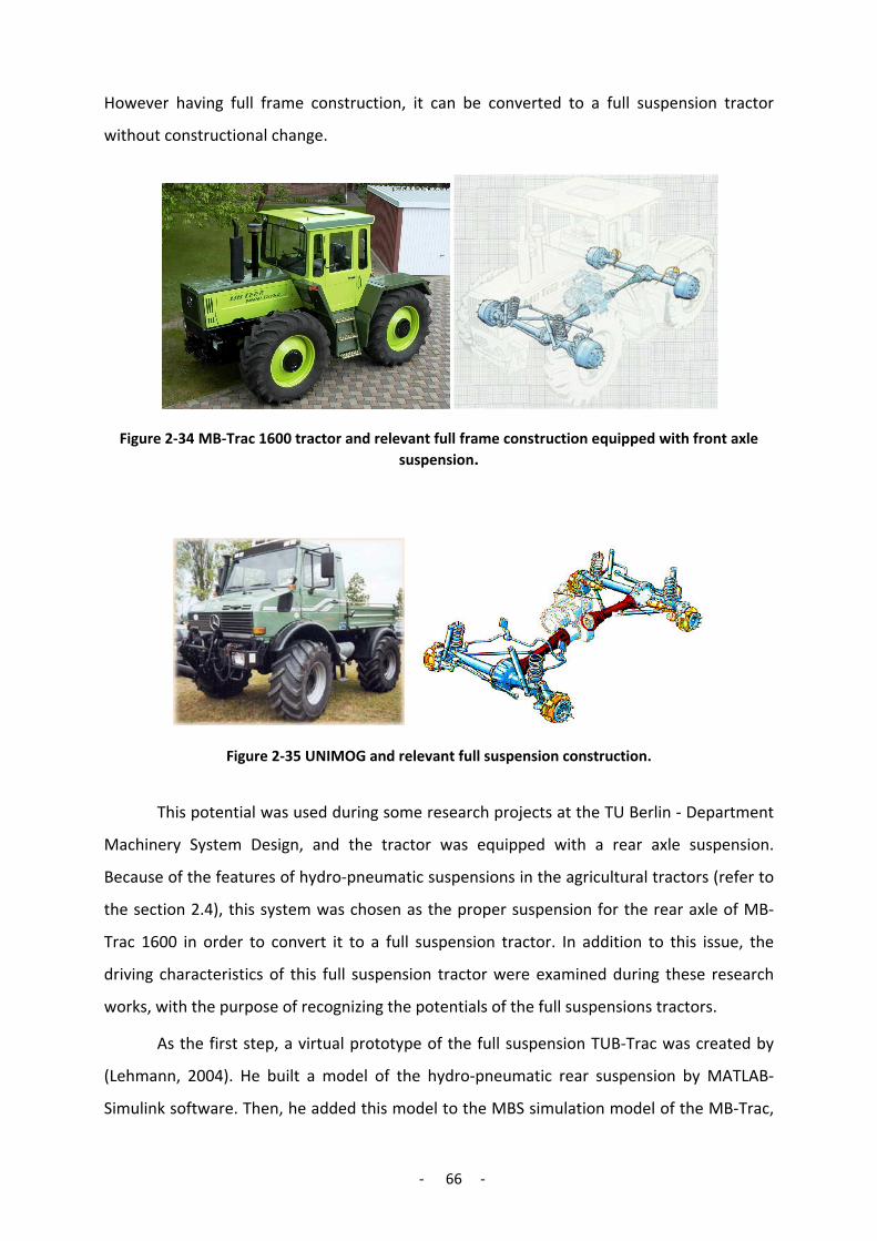
- 66 -

However having full frame construction, it can be converted to a full suspension tractor

without constructional change.

Figure 2-34 MB-Trac 1600 tractor and relevant full frame construction equipped with front axle suspension.

Figure 2-35 UNIMOG and relevant full suspension construction.

This potential was used during some research projects at the TU Berlin - Department

Machinery System Design, and the tractor was equipped with a rear axle suspension.

Because of the features of hydro-pneumatic suspensions in the agricultural tractors (refer to

the section 2.4), this system was chosen as the proper suspension for the rear axle of MB-

Trac 1600 in order to convert it to a full suspension tractor. In addition to this issue, the

driving characteristics of this full suspension tractor were examined during these research

works, with the purpose of recognizing the potentials of the full suspensions tractors.

As the first step, a virtual prototype of the full suspension TUB-Trac was created by

(Lehmann, 2004). He built a model of the hydro-pneumatic rear suspension by MATLAB-

Simulink software. Then, he added this model to the MBS simulation model of the MB-Trac,

- 67 -

which was made by “DADS” MBS software. By joining these two models together, he created

the overall model of the full suspension TUB-Trac. Finally, he performed some primary

simulation tests by using this model. In these tests, he considered four test modes: the

tractor without ballast, front ballast, rear ballast, and full ballast.

Figure 2-36 shows one of the results derived from these tests showing the frequency

response of the tractor in the two modes of the rear and front ballast. This graph indicates

that how the ballast of the tractor body influences on the natural frequency of the pitch

movement. At the end of this research work, it was recommended to employ the active

suspension systems, particularly the auto-leveling system. This system was considered for

the rear axle suspension of the tractor in order to improve its efficiency.

Figure 2-36 Amplitude spectrum of pitch movement of the tractor body for v=30 km (Lehmann, 2004).

After this model study, another research work was conducted by (Thiebes, Müller, &

Gericke, 2005) with the objective of preparing the MB-Trac for adding a hydro-pneumatic

suspension to its rear axle, including design and constructing a rear framework for it. Figure

2-37 shows the designed rear frame that was assembled to the main frame of the tractor.

Axle suspension was connected to this frame via a four bar linkage. This provides a degree of

freedom for the vertical movement of the axle. After this study, in the research work of

(Hoppe, 2006) the hydro-pneumatic rear suspension was designed and an actual prototype

was built, and then was installed on the MB-Trac tractor and in this way the full suspension

TUB-Trac was created. The details of this tractor and its rear suspension system will be given

in the next chapters.

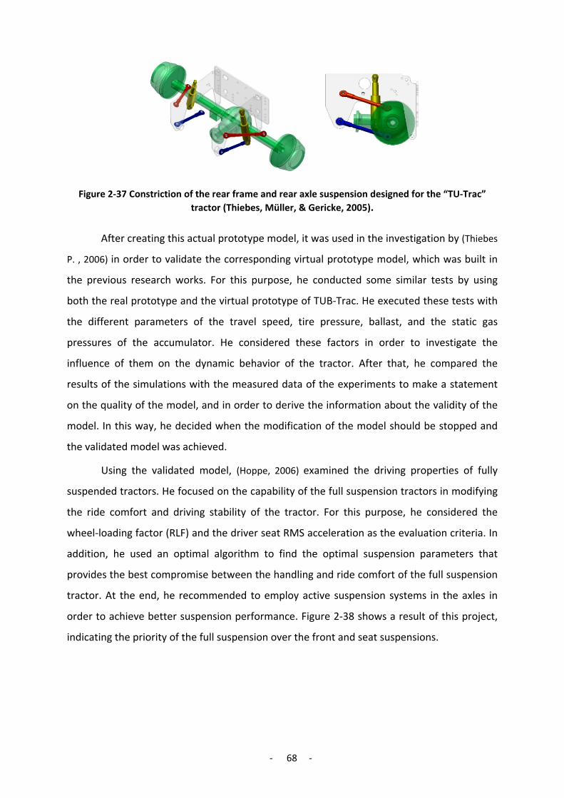
- 68 -

Figure 2-37 Constriction of the rear frame and rear axle suspension designed for the “TU-Trac” tractor (Thiebes, Müller, & Gericke, 2005).

After creating this actual prototype model, it was used in the investigation by (Thiebes

P. , 2006) in order to validate the corresponding virtual prototype model, which was built in

the previous research works. For this purpose, he conducted some similar tests by using

both the real prototype and the virtual prototype of TUB-Trac. He executed these tests with

the different parameters of the travel speed, tire pressure, ballast, and the static gas

pressures of the accumulator. He considered these factors in order to investigate the

influence of them on the dynamic behavior of the tractor. After that, he compared the

results of the simulations with the measured data of the experiments to make a statement

on the quality of the model, and in order to derive the information about the validity of the

model. In this way, he decided when the modification of the model should be stopped and

the validated model was achieved.

Using the validated model, (Hoppe, 2006) examined the driving properties of fully

suspended tractors. He focused on the capability of the full suspension tractors in modifying

the ride comfort and driving stability of the tractor. For this purpose, he considered the

wheel-loading factor (RLF) and the driver seat RMS acceleration as the evaluation criteria. In

addition, he used an optimal algorithm to find the optimal suspension parameters that

provides the best compromise between the handling and ride comfort of the full suspension

tractor. At the end, he recommended to employ active suspension systems in the axles in

order to achieve better suspension performance. Figure 2-38 shows a result of this project,

indicating the priority of the full suspension over the front and seat suspensions.

- 69 -

Figure 2-38 Comparison of the vertical acceleration present on the seat of TUB-Trac with three different suspension modes: seat, Front Suspension, and full suspension (Hoppe, 2006).

The main objective of the mentioned research works at the TU Berlin - Department

Machinery System Design was the improvement of the driving characteristics of the

agricultural tractors by using efficient suspension systems. Considering this objective, this

Ph.D. thesis was conducted with the theme of active suspension for the full suspension

tractors, as it was also recommended in the previous investigations. This project was

performed on the TUB-Trac, by applying an active suspension to the rear axle suspension of

this tractor, which was a hydro-pneumatic type.

2.5.8 Summary

In the previous sections, the characteristics of the different suspension systems of

agricultural tractors were described. In this part, these characteristics including positive and

negative features are summarized.

In order to determine the priority of the different suspension systems for agricultural

tractors, some research works has already been conducted. These investigations achieved

finally some useful results. However, they could not conclude directly about the priority of

the suspension systems. The reason was that they did not examine all these suspension

systems by similar tractors, but also they used different tractor models for each type of

suspension system. Since the qualities of the suspension systems in these tractors

independent of their type were not similar, it was not possible to achieve a clear conclusion

about the priority of suspension systems.

- 70 -

One of these investigations is the work of (Scarlett, Price, & Stayner, 2007) that was

conducted to the quantify emission of the whole-body vibration (WBV) of agricultural

tractors. For this purpose, exposure levels found upon a range of modern agricultural

tractors with different suspension systems were estimated. The considered systems were

seat suspension, seat plus cabin suspension, seat plus cabin plus front axle suspension, and

seat plus fully suspension. The evaluation tests were operated in some determined

conditions, and the test-tracks were the traversing ISO ride vibration types.

In addition, the conditions of performing selected agricultural operations and

performing identical tasks during ‘on-farm’ were considered. Finally in this investigation, the

whole RMS-results of the WBV for the different test conditions were presented. However,

the clear conclusion about the priority of the suspension systems was not achieved. It was

just founded that the emission-level of the WBV of tractors was very dependent upon the

nature of field operations, and in opposition, the emission-level was largely independent of

the capability of the vehicle suspension due to the dominance of the horizontal vibration.

However, during on-road transport, all these trends were reversed.

Based on the study about the different suspension systems used for agricultural

tractors, table 2-2 is derived, which shows a valuation of these systems. The judgment about

the capability of the suspension systems is issued based on their positive influence on the

ride comfort and handling of tractors. In addition, the complexity and the cost of adding the

suspension system to standard tractors is considered as a negative factor.

Table 2-2 The capability of different suspension systems used for agricultural tractors.

Suspension Influence on

Expenditure Ride Comfort Handling

Seat middle slight low

Cabin high low middle

Hitch low-middle low-high low

Front axle low high middle

Full axle high high high

As explanation of the grading for the suspension systems in this table, an abstract

about their capabilities and weaknesses are given again in this part. First systems are the

seat suspension systems that are relatively inexpensive and have robust construction. These

systems are the first choices in order to improve the ride comfort of tractors. Even if in

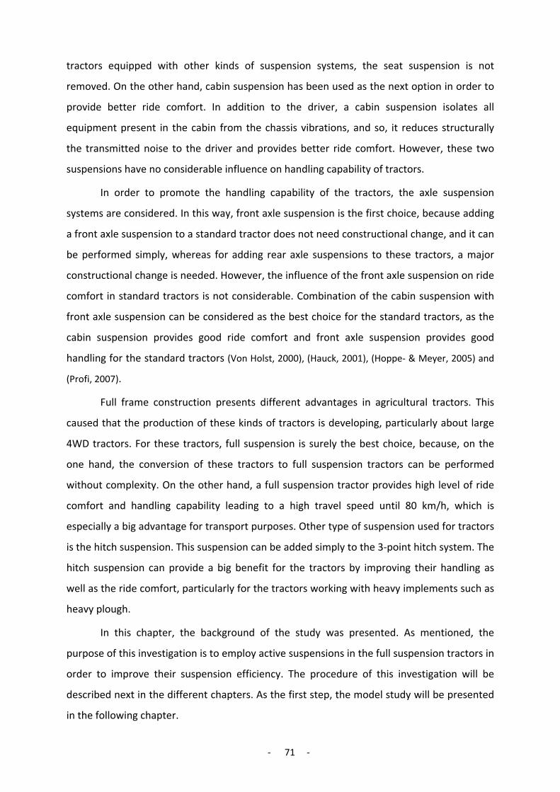
- 71 -

tractors equipped with other kinds of suspension systems, the seat suspension is not

removed. On the other hand, cabin suspension has been used as the next option in order to

provide better ride comfort. In addition to the driver, a cabin suspension isolates all

equipment present in the cabin from the chassis vibrations, and so, it reduces structurally

the transmitted noise to the driver and provides better ride comfort. However, these two

suspensions have no considerable influence on handling capability of tractors.

In order to promote the handling capability of the tractors, the axle suspension

systems are considered. In this way, front axle suspension is the first choice, because adding

a front axle suspension to a standard tractor does not need constructional change, and it can

be performed simply, whereas for adding rear axle suspensions to these tractors, a major

constructional change is needed. However, the influence of the front axle suspension on ride

comfort in standard tractors is not considerable. Combination of the cabin suspension with

front axle suspension can be considered as the best choice for the standard tractors, as the

cabin suspension provides good ride comfort and front axle suspension provides good

handling for the standard tractors (Von Holst, 2000), (Hauck, 2001), (Hoppe- & Meyer, 2005) and

(Profi, 2007).

Full frame construction presents different advantages in agricultural tractors. This

caused that the production of these kinds of tractors is developing, particularly about large

4WD tractors. For these tractors, full suspension is surely the best choice, because, on the

one hand, the conversion of these tractors to full suspension tractors can be performed

without complexity. On the other hand, a full suspension tractor provides high level of ride

comfort and handling capability leading to a high travel speed until 80 km/h, which is

especially a big advantage for transport purposes. Other type of suspension used for tractors

is the hitch suspension. This suspension can be added simply to the 3-point hitch system. The

hitch suspension can provide a big benefit for the tractors by improving their handling as

well as the ride comfort, particularly for the tractors working with heavy implements such as

heavy plough.

In this chapter, the background of the study was presented. As mentioned, the

purpose of this investigation is to employ active suspensions in the full suspension tractors in

order to improve their suspension efficiency. The procedure of this investigation will be

described next in the different chapters. As the first step, the model study will be presented

in the following chapter.

- 72 -

Chapter 3

3 Modeling of the Semi-active Suspension

In the previous chapters, the background and literature review of the investigation were

presented, and the proper active suspension and related control strategy for this

investigation were determined. In addition, it was proposed that the new suspension system

is examined by applying it to a test agricultural tractor. This examination was not performed

only by a practicable experience, but also a computer simulation was planned in order to

examine the new system. For this purpose, a computer model of all system components is

needed. This chapter explains the details of this modeling.

The total model includes two main components. The first one is the model of the semi-

active suspension including three sub-models: controller model, actuator model, and sensor

model. This semi-active suspension is applied to the test-tractor. Therefore, the second

model component is the model of this test-tractor. In figure 3-1, the structure is illustrated.

As shown, the whole system works in a close loop. The dynamic behavior of the tractor is

scanned by the sensors. After that, this information is sent to the controller. Based on the

relevant control strategy, the controller sends the commands to the actuator and in this way,

changes the parameters of the tractor suspension.

Figure 3-1 Control loop in a tractor with active suspension system.

For modeling of the components, a similar routine is used. Figure 3-2 illustrates the

four steps of the modeling process. In the first step, the real system is known in details. Then

Test-Tractor

Sensors

Controller Actuator Suspension Tractor

Dynamics

- 73 -

based on this knowledge, the physical model of the system is created, and after that by

deriving the equation of this model, the mathematical model is produced. In the last step,

the computer model is developed from the model equations by using MATLAB-Simulink

program.

Figure 3-2 Modeling procedure.

The modeling part of the research project is performed in three steps. At the first step,

the model of the tractor is built. Then, the model of the actuator system including the hydro-

pneumatic rear suspension of the tractor is created. In the last step, the controller and

sensors are modeled. In conclusion, after all these steps, the simulation model is developed

by connecting all models together.

3.1 Full Vehicle Model

In the first step of the modeling, the full vehicle model of the tractor is developed. This

model includes the sub-models of the tire, tractor body, wheels, and tractor suspension,

which will be explained in this part.

3.1.1 Tire Model

Tires are the first elastic element between the road surface and vehicle that have an

important role in providing effective isolation from the road disturbances, particularly the

high frequency road input that is not damped effectively by a suspension system. On the

other hand, the tires characteristics are related closely to the quality of the tire-road contact

and the vehicle handling.

A precise modeling of tires is complicated, because the stiffness and the damping

characteristics of tires are not constant and are affected by different factors such as static

load, inner pressure, temperature, rotational speed, and excitation frequency (Von Holst,

2000). In order to consider all these effects, some complicated models are presented. For

example, some of them use FEM modeling that defines a little bit of the tire as the basic

element of the modeling. In this way, they consider the effect of the vertical, lateral, and

longitudinal tire forces and also, the effect of these forces on one another (Blundell, 1999).

Real System Physical Model

Mathematical Model

Computer Model

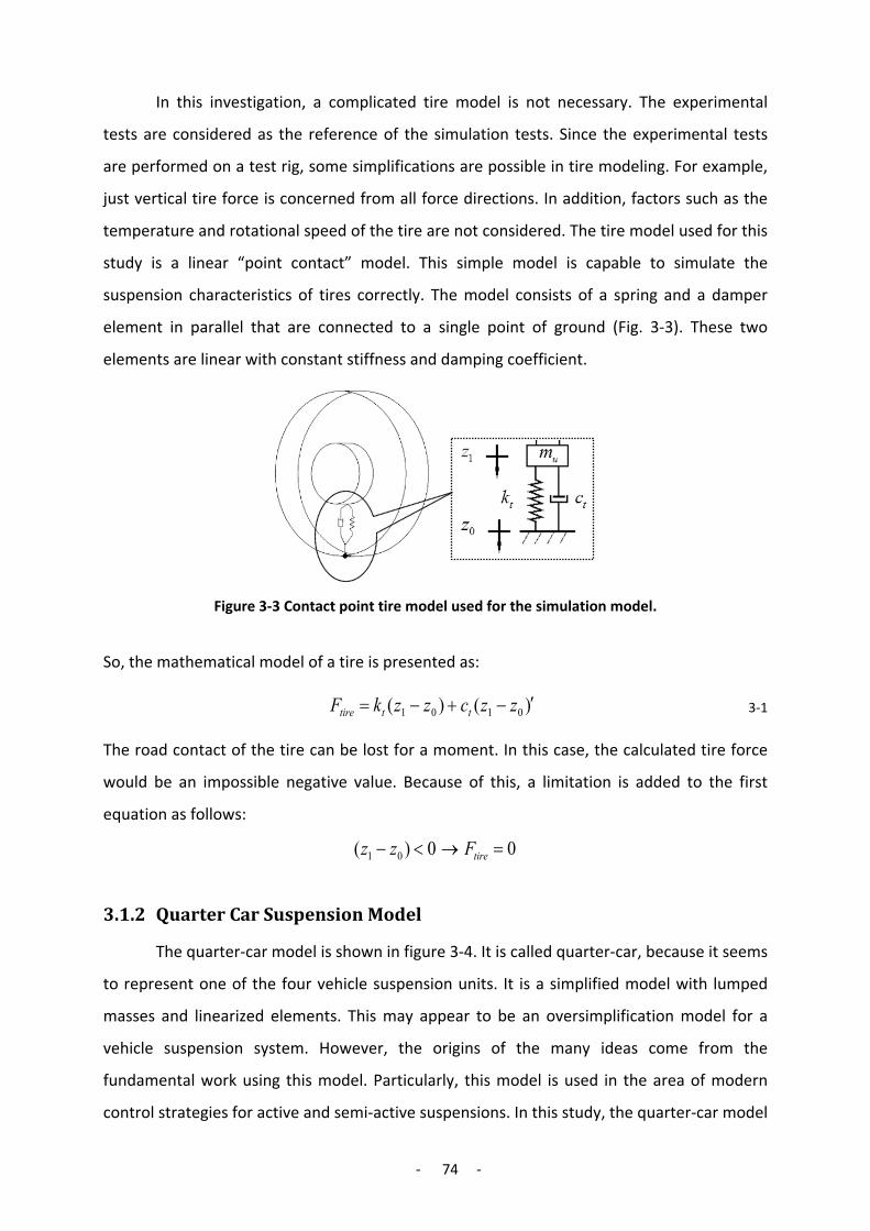
- 74 -

In this investigation, a complicated tire model is not necessary. The experimental

tests are considered as the reference of the simulation tests. Since the experimental tests

are performed on a test rig, some simplifications are possible in tire modeling. For example,

just vertical tire force is concerned from all force directions. In addition, factors such as the

temperature and rotational speed of the tire are not considered. The tire model used for this

study is a linear “point contact” model. This simple model is capable to simulate the

suspension characteristics of tires correctly. The model consists of a spring and a damper

element in parallel that are connected to a single point of ground (Fig. 3-3). These two

elements are linear with constant stiffness and damping coefficient.

Figure 3-3 Contact point tire model used for the simulation model.

So, the mathematical model of a tire is presented as:

)()( 0101 ′−+−= zzczzkF tttire 3-1

The road contact of the tire can be lost for a moment. In this case, the calculated tire force

would be an impossible negative value. Because of this, a limitation is added to the first

equation as follows:

00)( 01 =→<− tireFzz

3.1.2 Quarter Car Suspension Model

The quarter-car model is shown in figure 3-4. It is called quarter-car, because it seems

to represent one of the four vehicle suspension units. It is a simplified model with lumped

masses and linearized elements. This may appear to be an oversimplification model for a

vehicle suspension system. However, the origins of the many ideas come from the

fundamental work using this model. Particularly, this model is used in the area of modern

control strategies for active and semi-active suspensions. In this study, the quarter-car model

- 75 -

is also used as basics for deriving of the full vehicle. The fundamental parameters of a

suspension system can be defined by this model. These parameters are presented in table 3-

1.

Figure 3-4 Quarter-car model and relevant free body diagram.

Table 3-1 Quarter-car suspension model parameters.

Symbols Description Symbols Description

1m Unsprung mass (i.e. wheel assembly) 1z Unsprung mass displacement

2m Sprung mass (i.e. vehicle body) 2z Sprung mass displacement

2k Suspension stiffness 0z Road input displacement

2c Suspension damping )( 12 zz − Suspension travel

1k Tire stiffness )( 01 zz − Tire deflection

1c Tire damping

Figure 3-4 shows the free body diagram of the quarter-car model. Looking at this

model, the equations of the sprung mass and unsprung mass motions can be derived in two

parts as follow:

First, sprung mass equation,

0)()(

0

12212222

22 22

=′−′+−+″+

=++″+

zzczzkzm

FFzm ck 3-2

Then, unsprung mass equation,

0)()()()(

0

12212201101111

11 2211

=′−′−−−′−′+−+″+

=−−++″+

zzczzkzzczzkzm

FFFFzm ckck 3-3

- 76 -

The motions of the sprung and unsprung masses ),..( 21 zzei can be determined by solving

the system of these two differential equations. In the following sections, full-tractor

suspension model will be described. The quarter-car model and relevant equations will be

used as the basics of this full-tractor model.

3.1.3 Full-Vehicle Model Degrees of Freedom

The quarter-car model can be used in order to evaluate the main characteristics of

vehicle suspensions. However, a model with the two degrees of freedom of the sprung and

unsprung masses covers just the vertical motions of a vehicle, and in order to study the

rotational motions, other models with more degrees of freedom are necessary. A full-vehicle

model is able to cover all needed degrees of freedom. As before, it is necessary to define a

proper coordinate system for dynamics of a tractor.

For this purpose, there are two kinds of coordinate systems: space-fixed and vehicle-

fixed system. The first one fixing at one point in space determines the position and

orientation of a vehicle. This system is used in order to define the maneuver path of a

vehicle. In opposition, vehicle-fixed coordinate system is originated at the center of gravity

(CG) of a vehicle and travels with it. In the study of suspensions, the vehicle-fixed system is

used in order to define a relative coordinate system for the dynamics of the suspension

components. This coordinate system is shown in figure 3-5.

Figure 3-5 Vehicle-fixed coordinate system.

According to the ISO convention, the positive directions of the axes are defined as follow:

1- x-axis: straight to the forward from the vehicle.

- 77 -

2- y-axis: straight to the left from the vehicle.

3- z-axis: straight to the upwards from the vehicle.

Now with respect to the vehicle fixed coordinate system, the vehicle motions can be

described. There are six degrees of freedom (6DOF) related to the vehicle body motions

including three dimensional and three rotation degrees of freedom. In addition, there are

four dimensional degrees of freedom related to the unsprung masses, which is the number

of the vehicle wheels. These vehicle motions and relevant terminology are mentioned

frequently in this thesis. Thus, these motions of the vehicle body are described in this part.

Table 3-2 illustrates the list of the complete degrees of freedom for a four-wheel vehicle.

These degrees of freedom are explained as follow:

1- Longitudinal: It is the body motion in x-axis dimension or forward/backward. For

example as a vehicle accelerates or brakes, its body is exited with forces in this direction

called longitudinal forces.

2- Lateral: It is the body motion in y-axis dimension or left/right. An example for this

direction is the centrifugal lateral force entering to the vehicle during turning.

Table 3-2 Vehicle degrees of freedom.

No. Vehicle

Part Degree of Freedom Motion Axis

1 body longitudinal dimension x-axis

2 body lateral dimension y-axis

3 body vertical(heave) dimension z-axis

4 body roll rotation x-axis

5 body pitch rotation y-axis

6 body yaw rotation z-axis

7 wheel-1 vertical dimension z-axis

8 wheel-2 vertical dimension z-axis

9 wheel-3 vertical dimension z-axis

10 wheel-4 vertical dimension z-axis

3- Vertical: It is the body motion in z-axis dimension or up/down. Upward and

downward motion of the vehicle body caused by uneven road is an example for this case.

This motion is also referred to as "heave" or in some references as "bounce”. This motion is

usually measured at the mass center of the vehicle body and is considered as an important

- 78 -

parameter of the performance of a suspension. Among these three-dimensional motions of

the vehicle body, just vertical direction is related to the suspension operation, and because

of this, only this motion is studied in modeling of the tractor.

4- Roll: It is the rotation body motion about x-axis (Fig. 3-6 and 3-7). Leaning of the

vehicle body during cornering is an example for the excitation of the roll motion. As a vehicle

turns a corner, the centrifugal force entering to the vehicle body is resisted by the tires road

contact force. Interaction of these two forces creates torque at the vehicle body that causes

a vehicle weight transfer on one side, and the vehicle leans consequently towards the

outside of the curve. This is what is called body roll. The extreme amplitude of the body roll

causes a critical situation for vehicle stability. The performance of the suspension system has

the main role in providing the roll stability for a vehicle.

5- Pitch: It is the rotation body motion about y-axis (Fig. 3-6 and 3-7). The dive of the

vehicle body during braking is a typical example for the excitation of the pitch body motion.

As a vehicle brakes, the inertia of the vehicle body causes transfer of the center of gravity

(CG) of the body, and vehicle dives forward, and the weight on the rear tires transfers to the

front tires. This causes a critical moment in controlling of a vehicle.

6- Yaw: It is the rotation body motion about z-axis (Fig. 3-6 and 3-7). The spinning

motion of a vehicle is an example for the yaw motion. This instability mode may occur during

cornering on slippery surfaces. In this situation, the decreased traction forces of the rear

tires are not able to resist against centrifugal force, and tires slip, and vehicle turns violently

around itself. This body motion is not related directly to the suspension system of a vehicle,

and so that, it is not considered in the full-tractor model.

7- Wheel hop: It is the unsprung mass motion in z-axis dimension or up/down. In

addition to the body motions, the wheel motion is also important in the study of vehicle

dynamics. This motion is in z-axis direction and referred usually as “wheel hop”. This motion

affects directly the tire-road connections and influences consequently the vehicle stability.

Using the definitions of the coordinate systems and vehicle motions, physical model of the

tractor will be derived in the following sections.

3.1.4 Physical Full Vehicle Model

As mentioned before, a quarter-car model is not able to simulate all important

vehicle motions considered in the suspension system. Thus, another model with more

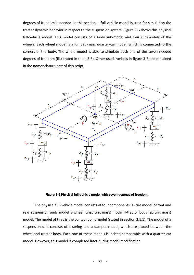
- 79 -

degrees of freedom is needed. In this section, a full-vehicle model is used for simulation the

tractor dynamic behavior in respect to the suspension system. Figure 3-6 shows this physical

full-vehicle model. This model consists of a body sub-model and four sub-models of the

wheels. Each wheel model is a lumped-mass quarter-car model, which is connected to the

corners of the body. The whole model is able to simulate each one of the seven needed

degrees of freedom (illustrated in table 3-3). Other used symbols in figure 3-6 are explained

in the nomenclature part of this script.

Figure 3-6 Physical full-vehicle model with seven degrees of freedom.

The physical full-vehicle model consists of four components: 1- tire model 2-front and

rear suspension units model 3-wheel (unsprung mass) model 4-tractor body (sprung mass)

model. The model of tires is the contact point model (stated in section 3.1.1). The model of a

suspension unit consists of a spring and a damper model, which are placed between the

wheel and tractor body. Each one of these models is indeed comparable with a quarter-car

model. However, this model is completed later during model modification.

- 80 -

Table 3-3 Considered degrees of freedom in the full-vehicle model.

Nr. Symbol Description

1 θ pitch angle at center of gravity

2 ϕ roll angle at center of gravity

3 cgz heave displacement at center of gravity

4 flz1 front-left unsprung mass vertical displacement

5 frz1 front-right unsprung mass vertical displacement

6 rlz1 rear-left unsprung mass vertical displacement

7 rrz1 rear-right unsprung mass vertical displacement

Similar to the procedure of all other modeling, there are some assumptions and

simplifications in this modeling. The tractor axles are like a link between the right and left

units. In spite of this, in the models of the unsprung masses, it is assumed that the

suspension units are independent, and the effects of the axles are ignored. Similar to

quarter-car model, the unsprung mass is considered as lumped-mass. The parameters of the

unsprung mass are calculated by adding the wheel mass and a part of the axle mass.

In full vehicle model, tractor body is also modeled as a rectangular form of lumped-

mass models. This mass form has specific dimensions determining the position of the center

of gravity and position of the four suspension units standing on the corners of the body. In

this modeling, it is also supposed that the axes of the roll and pitch cross the center of

gravity (Fig. 3-5). This model presents a proper simplification. However, it is needed that the

related mass and inertia parameters to be calculated accurately. In the reality, tractor body

involves different masses standing on different position. In order to accurate the model

parameters, the body of the tractor is considered a multi-rigid body mass. This mass consists

of some main mass-components such as engine, chassis, transmission, and cabin.

In appendix E1, there are more information about the parameters of the rigid multi-

body model including the mass and position of the body components. In addition, the

methods of calculating total mass and moment of inertia are indicated. It should be also

considered that the body model is still a solid model, and there is no consideration for elastic

connections among body components. In the following section as the next step of modeling,

equations derivation of the model will be explained.

- 81 -

3.1.5 Mathematical Full Vehicle Model

In mathematical modeling, the suspension between the tractor body and wheels are

modeled by simple linear spring and damper elements, whereas some of these elements in

the test-tractor are hydraulic or hydro-pneumatic elements with non-linear characteristic.

Using simple linear model for these elements provides proper simplifications for the primary

full tractor model. In the following steps of the modeling, the non-linear elements will be

modeled separately. Then, these new models will be replaced with the simple primary

models.

In mathematical modeling, the motion equations for each one of seven degrees of

freedom are derived. These motions are four unsprung masses motions along with the three

motions of the sprung mass. As the first stage, the differential equations of the tractor’s four

unsprung masses are derived based on the equations of the quarter-car model (refer to

section 3.1.2). The equations of the tractor’s four unsprung masses are with respect to figure

3-6 as follow:

0)()()()(

:

121201011 =−−′−−−+′−+″+ flflflflflflflfltfflfltffluf zzkzzczzkzzczm

fl 3-4

0)()()()(

:

121201011 =−−′−−−+′−+″+ frfrfrfrfrfrfrfrtffrfrtffruf zzkzzczzkzzczm

fr

0)()()()(

:

121201011 =−−′−−−+′−+″+ rlrlrlrlrlrlrlrltrrlrltrrlur zzkzzczzkzzczm

rl

0)()()()(

:

121201011 =−−′−−−+′−+″+ rrrrrrrrrrrrrrrrtrrrrrtrrrur zzkzzczzkzzczm

rr

After the unsprung mass, equations of the unsprung mass are derived. For this

purpose at first, the unsprung mass motion on the center of gravity is decomposed to the

three components: heave, pitch, and roll motions. After that, the equations of all motions

are derived separately, and finally by adding the effect of all these motions, the equations of

the body motions are achieved. First, it is supposed that the displacements are small (i.e. Sin

α ≈ α.). The equations are derived similar to sprung mass equation in the quarter-car model

(refer to equation 3-2).For each equation, the effects of all four unsprung mass forces are

considered.

- 82 -

After some manipulations, these equations are presented as follow:

Heave,

1 2 1 2 1 2 1 2

1 2 1 2 1 2 1 2

1 [ ( ) ( ) ( ) ( )

( ) ( ) ( ) ( )]

cg fl fl fl fl fl fl fr fr fr fr fr frt

rl rl rl rl rl rl rr rr rr rr rr rr

z c z z k z z c z z k z zm

c z z k z z c z z k z z

″ ′ ′= + − + − + − + − +

′ ′− + − + − + − 3-5

Pitch,

2 1 2 1 2 1 2 1

2 1 2 1 2 1 2 1

1 [ ( ) ( ) ( ) ( )

( ) ( ) ( ) ( )]

f fl fl fl f fl fl fl f fr fr fr f fr fr fryy

r rl rl rl r rl rl rl r rr rr rr r rr rr rr

l c z z l k z z l c z z l k z zI

l c z z l k z z l c z z l k z z

θ ′′ ′ ′= + ⋅ − + ⋅ − + ⋅ − + ⋅ − +

′ ′− ⋅ − − ⋅ − − ⋅ − − ⋅ −

3-6

Roll,

2 1 2 1 2 1 2 1

2 1 2 1 2 1 2 1

1 [ ( ) ( ) ( ) ( )

( ) ( ) ( ) ( )]

l fl fl fl l fl fl fl r fr fr fr r fr fr frxx

l rl rl rl l rl rl rl r rr rr rr r rr rr rr

t c z z t k z z t c z z t k z zI

t c z z t k z z t c z z t k z z

ϕ′′ ′ ′= − ⋅ − − ⋅ − + ⋅ − + ⋅ − −

′ ′⋅ − − ⋅ − + ⋅ − + ⋅ − 3-7

After all by considering the dimensions of the tractor body (Fig. 3-6), the effect of all these

sprung mass motions are added together in order to calculate the vertical accelerations of

the body’s corners as follows:

⎩⎪⎪⎨

⎪⎪⎧

ϕθ ′′+′′−′′=′′ ..z2fl lfcg tlz

ϕθ ′′−′′−′′=′′ ..z2fr rfcg tlz

ϕθ ′′+′′+′′=′′ ..z2rl lrcg tlz

ϕθ ′′−′′+′′=′′ ..z2rr rrcg tlz

� 3-8

In this section, the mathematical full-vehicle model was created. This model included the

equations of the vertical or rotational motion of the unsprung masses (i.e. wheels) and

sprung mass (i.e. body). These equations will be used as the basics of the full-vehicle

computer model presenting in the next section.

3.1.6 Simulink Full Vehicle Model

Figure 3-7 shows the computer model of the mathematical full vehicle model created

by MATLAB-Simulink program. This model consists of the two sub-models: unsprung mass

and sprung mass. Because of the direct relation between these two masses, their models are

also joined together. The input of the model is a road profile that enters to the unsprung

mass sub-model. Outputs of the model are some model variables that are used in order to

- 83 -

evaluate the suspension. In addition, some of these variables are used as the input of the

controller. These inputs and outputs of the model will be described in the next sections.

Figure 3-7 Full vehicle Simulink model.

The sprung mass model is shown in figure 3-8. This model simulates the motions of

the vehicle sprung mass. As explained before about the mathematical model, the sprung

motion is decomposed initially to the heave, pitch, and roll motions. As shown in this figure,

the Simulink model consists of three blocks: heave, pitch, and the roll motions of the sprung

mass. These blocks are based on the equation 3-5, 3-6, and 3-7.

The motions are summed by the “sum” block, which is based on equation 3-8. In

addition, this block produces the displacements and velocities of the vertical motion of the

body corners, which are used as the inputs of the unsprung mass model. Unsprung mass

model is shown in figure 3-9. This model simulates the vertical motions of the four vehicle

wheels. As shown in this figure, this model consists of the four blocks of the unsprung

masses of the vehicle created based on the equation 3-4.

As conclusion, the full vehicle simulink model of the tractor was presented in this

section. This model is used as the foundation of the overall model. As shown in figure 3-1,

the overall model consists of some other components that will be added to the full vehicle

Simulink model later. These rest components will be presented in the following sections of

this chapter.

- 84 -

Figure 3-8 Vehicle sprung mass Simulink model.

Figure 3-9 Vehicle unsprung mass Simulink model.

Heave

Pitch

Roll

- 85 -

3.1.7 Front Suspension Model

The dampers of the tractor front suspension are hydraulic dampers with non-linear

characteristic. In the full vehicle model, these dampers are simulated with a simple linear

model to prevent the model equations from complication. After building the Simulink full

vehicle model, a more accurate model for the dampers of the front suspension are

presented in this section. Figure 3-10 shows the force-velocity characteristic of these

dampers. This graph is achieved from the experimental data of the real damper, presenting

the real characteristic of the dampers.

Figure 3-10 Measured force-velocity characteristic of the dampers used for the front axle of the test-tractor.

By inserting this information into a Simulink “Lookup Table”, a one-dimensional

function is created to approximate the damper force with respect to the damper cross

velocity. This new function replaces the primary simple linear function, and so, an accurate

model for the damper is provided. Figure 3-11 shows the use of this new damper model in

the full vehicle Simulink model.

After the modification of the front suspension model, derivation of a more accurate

model is considered for the hydro-pneumatic rear suspension. This model is an important

part of the overall model, because it is indeed the actuator system of the semi-active

suspension. In the following sections, the parts of this modeling will be described.

-4

0

4

8

12

16

-4 -3 -2 -1 0 1 2 3 4

Forc

e [K

N]

Velocity (m/s)

- 86 -

Figure 3-11 Damper model of the front suspension in full vehicle Simulink model.

3.2 Actuator Model

In a vehicle with an active suspension system, the actuators are the components that

work between the controller and the tractor suspension (refer to Fig. 3-1). It receives the

control commands from the controller and applies the forces to the suspension. In this way,

it can modify the vehicle dynamics. The actuator is indeed a part of an active suspension

system with the parameters that can be changed by the command of a controller. In this

investigation, the semi-active suspension system is used for the hydro-pneumatic rear

suspension of the test-tractor. The variable damper of this hydro-pneumatic suspension is

indeed the actuator of the system. Using this part, the damping level of the suspension can

be changed by the order of the controller.

Figure 3-12 A variable hydro-pneumatic suspension as the actuator of the system.

Hydro-pneumatic suspension can be modeled as a set consists of a spring and a

damper. The stiffness effect of the system creates by the compressed gas of the

accumulator, and the damping effect of the system creates by throttling the flowing oil

between the cylinder and accumulator. In order to use this system as the actuator, a

- 87 -

controllable throttle is added to this system (Fig. 3-12). In order to build the model, the

function of the actuator is divided into the two parts of the spring and variable damper. The

first part generates the stiffness force and the second one generates the controllable force

damping force of the suspension. These two components are modeled separately. By joining

these two models, the hydro-pneumatic actuator model is created.

3.2.1 Hydro-Pneumatic Spring Model

The stiffness effect of a hydro-pneumatic suspension is produced by compressing the

gas in accumulators. The hydro-pneumatic cylinder forces oil to the accumulator and

compress the gas inside the accumulator. The produced pressure is transferred to the

cylinder via a pipe. This pressure is proportional to the piston displacement. Therefore,

stiffness force is produced in the cylinder. In the hydro-pneumatic suspension of the test-

tractor, a double-acting cylinder is used (Figure 3-13). Both side of this cylinder are

connected to two accumulators, which generate the stiffness force of the suspension.

Figure 3-13 Spring component of a hydro-pneumatic suspension with a double-acting

cylinder.

By removing the throttle from a hydro-pneumatic suspension, only the stiffness

effect is remained. In the following sections, the spring components of the hydro-pneumatic

suspension will be modeled. First, the cylinder and accumulator are modeled separately.

Then, these two models are joined together in order to create the model of the hydro-

pneumatic spring.

3.2.1.1 Cylinder

In a hydro-pneumatic suspension, the cylinder converts the hydraulic pressure to the

stiffness and damping forces. Then, the cylinder producing the stiffness and damping forces

works alone instead of both the spring and damper in a conventional suspension. The

cylinders used in the hydro-pneumatic suspension of the test-tractor are a double-acting

- 88 -

cylinder. Respecting to figure 3-14, the parameters and variables of the cylinder are

presented in table (3-4).

Figure 3-14 A double-acting hydraulic cylinder.

Table 3-4 The parameters and variables definition of the double-acting hydraulic cylinder.

Variable Symbol Parameter Symbol

travel, velocity, force Fvx ,, piston area (head side) 1A

pressure head/rod side 21, PP piston area (rod side) 2A

volume, head/rod side 21,VV

flow rate, head/rod side 21,QQ

The relations between these parameters and variables are presented by the following

formulas:

2211 ApApF ⋅−⋅= 3-9

vAQvAQ ⋅=⋅= 2211 , 3-10

xAVxAV ∆⋅−=∆∆⋅=∆ 2211 , 3-11

Based on these formulas, the Simulink model of the double-acting cylinder is built

(Fig. 3-15). This model is used as a component of the spring model. As shown, the outputs of

this model are: cylinder force, cylinder volume alternation, and cylinder volume flow rate.

The force is indeed the output of the suspension, and volume alternation output is

connected to the accumulator model. The output of the volume flow rate of the cylinder is

also applied to the throttle model. The inputs of the cylinder model are the cylinder

pressures, piston displacement, and velocity. The dynamics inputs are the functional road

inputs, and the pressure input comes from the accumulator model.

- 89 -

Figure 3-15 Simulink model of the double-acting cylinder.

3.2.1.2 Accumulator

As oil enters to an accumulator, the gas inside the accumulator becomes

compressed. In this way, the accumulator is used in the hydraulic systems in order to reserve

the pressurized oil. In a hydro-pneumatic suspension, the accumulator is connected to the

cylinder, and the cylinder converts the oil pressure of the accumulator to the spring force.

Accumulators have a dynamic function in a hydro-pneumatic suspension. Therefore, the

bladder-type of accumulators is employed in the tractor suspension (Fig. 3-16). The

parameters and variables of the accumulator are presented in table 3-5.

Figure 3-16 A bladder accumulator using in hydro-pneumatic suspensions.

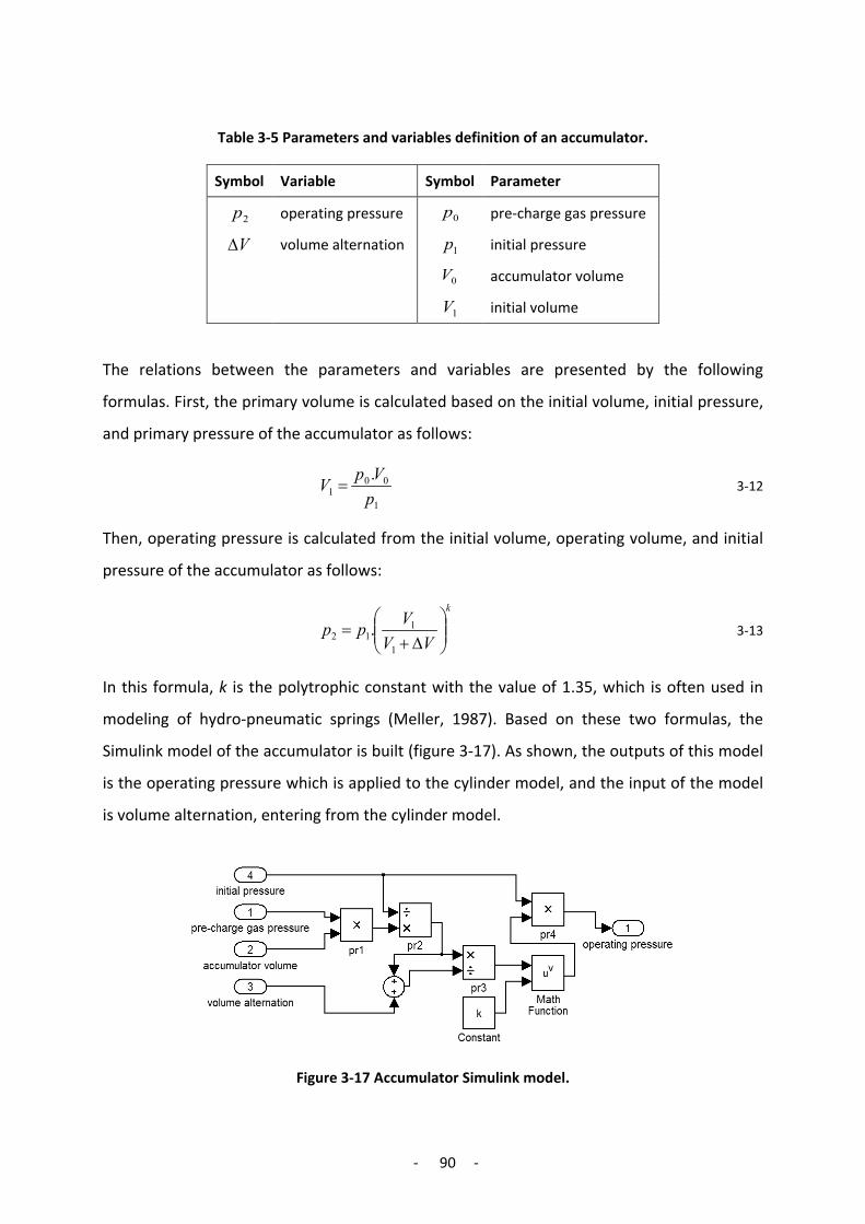
- 90 -

Table 3-5 Parameters and variables definition of an accumulator.

Parameter Symbol Variable Symbol

pre-charge gas pressure 0p operating pressure 2p

initial pressure 1p volume alternation V∆

accumulator volume 0V

initial volume 1V

The relations between the parameters and variables are presented by the following

formulas. First, the primary volume is calculated based on the initial volume, initial pressure,

and primary pressure of the accumulator as follows:

1

001

.pVpV = 3-12

Then, operating pressure is calculated from the initial volume, operating volume, and initial

pressure of the accumulator as follows:

k

VVVpp

∆+

=1

112 . 3-13

In this formula, k is the polytrophic constant with the value of 1.35, which is often used in

modeling of hydro-pneumatic springs (Meller, 1987). Based on these two formulas, the

Simulink model of the accumulator is built (figure 3-17). As shown, the outputs of this model

is the operating pressure which is applied to the cylinder model, and the input of the model

is volume alternation, entering from the cylinder model.

Figure 3-17 Accumulator Simulink model.

- 91 -

3.2.1.3 Spring Model

After building the models of the cylinder and accumulator, these two models are

joined together to create the hydro-pneumatic spring model (Fig. 3-18).

Figure 3-18 Simulink model of the hydro-pneumatic spring.

Figure 3-19 Stiffness-displacement curve of the hydro-pneumatic spring model.

As shown, the volume outputs of the cylinder are connected to the volume inputs of

the accumulator, and the pressure outputs of the accumulator are connected to the pressure

inputs of the cylinder. The output and input of the overall model of the hydro-pneumatic

spring are the displacement and force. These parameters are identical to the output and

input of a typical spring model.

- 92 -

In order to demonstrate the simulation characteristic of the hydro-pneumatic spring,

the stiffness-displacement curve of the overall model is created by applying the simulation

parameters (Fig. 3-19). Unlike a conventional spring, the stiffness is not constant and rises

progressively with increasing of the spring displacement. After modeling of the hydro-

pneumatic spring, the next step is to derive the model of the hydro-pneumatic variable

damper presented in the next sections.

3.2.2 Hydro-pneumatic Variable Damper Model

In a hydro-pneumatic suspension, the damping effect is created by using a throttle

between the cylinder and accumulators (Fig. 3-20). As oil flows through this throttle, a

pressure drop proportional to the flow rate is created. This pressure appears on the piston as

the damping force, which is proportional to the piston velocity and the. In a hydro-

pneumatic suspension with semi-active control, damping force is controllable by using a

variable throttle.

Figure 3-20 Using a variable throttle in hydro-pneumatic suspension in order to create a variable damping effect.

After modeling of the spring component, the variable damper is modeled to

complete the overall model of the actuator. The variable damping system and the relevant

derived models are described in the following sections.

3.2.2.1 On-off Damper Structure

There are two kinds of actuator systems in semi-active suspensions: continuous and

on-off variable damper. The used system in this study is on-off damper, which works in just

two levels of low and high damping. Figure 3-21 shows the hydro-pneumatic suspension unit

of the tractor including the variable on-off damping system. The components of this system

are presented in table 3-6.

- 93 -

Figure 3-21 On-off damper components of the hydro-pneumatic suspension unit.

Table 3-6 On-off damper components.

Description Symbol

cylinder ports 11, rh TT

throttles 22 , rh TT

valves rh VV ,

The throttles and valves are attached together in parallel, and they stand between

the cylinders and accumulators. As a valve is turned off, the oil flows through both the

throttle and cylinder port, and damping effect is created by both of them (Fig. 3-22-a). In

opposition, as the valve is on, the oil flows through the parallel valve as well as the throttle.

This deports the damping effect of the throttle from the system. Therefore, the damping

effect in this mode is created just by cylinder port, and the lower damping level is created in

this way (Fig. 3-22-b). To sum up, the “off” valve creates the high damping level, and “on”

valve creates the low damping level in the suspension system.

Figure 3-22 On-off damper system with two level of a) high and b) low damping.

b) a)

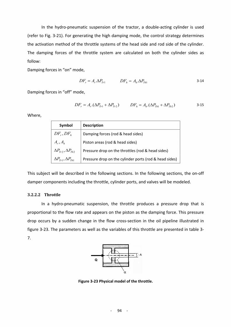
- 94 -

In the hydro-pneumatic suspension of the tractor, a double-acting cylinder is used

(refer to Fig. 3-21). For generating the high damping mode, the control strategy determines

the activation method of the throttle systems of the head side and rod side of the cylinder.

The damping forces of the throttle system are calculated on both the cylinder sides as

follow:

Damping forces in “on” mode,

3-14 1. Thhh PADF ∆= 1. Trrr PADF ∆=

Damping forces in “off” mode,

3-15 ).( 21 ThThhh PPADF ∆+∆=

).( 21 TrTrrr PPADF ∆+∆=

Where,

Description Symbol

Damping forces (rod & head sides) hr DFDF ,

Piston areas (rod & head sides) hr AA ,

Pressure drop on the throttles (rod & head sides) 22 , ThTr PP ∆∆

Pressure drop on the cylinder ports (rod & head sides) 11, ThTr PP ∆∆

This subject will be described in the following sections. In the following sections, the on-off

damper components including the throttle, cylinder ports, and valves will be modeled.

3.2.2.2 Throttle

In a hydro-pneumatic suspension, the throttle produces a pressure drop that is

proportional to the flow rate and appears on the piston as the damping force. This pressure

drop occurs by a sudden change in the flow cross-section in the oil pipeline illustrated in

figure 3-23. The parameters as well as the variables of this throttle are presented in table 3-

7.

Figure 3-23 Physical model of the throttle.

- 95 -

Table 3-7 Parameters and variables of the throttle.

Parameter Symbol Variable Symbol

throttle cross-section A volumetric flow rate Q

density of the oil ρ pressure drop p∆

flow reference number α

The following equation presents a proper mathematical model for a throttle (Festo, 2003).

22

2

..2.

AQp

αρ

=∆ 3-16

As shown, pressure drop of a throttle is directly proportional to the square of the flow rate.

Based on this formula, the Simulink model of the throttle is derived (Fig. 3-24).

Figure 3-24 Simulink throttle model.

In this model, flow rate and pressure drop are the input and output of the model,

which are connected to the cylinder model of the hydro-pneumatic suspension. The input of

the flow rate is provided from the output of the cylinder model, and the pressure drop of the

throttle is added to the pressure input of the cylinder model.

3.2.2.3 Cylinder Port

Cylinder ports are the outlet and inlet of a hydraulic cylinder (Fig. 3-25).

Figure 3-25 Hydraulic ports of a double-acting cylinder.

- 96 -

As mentioned before, ports of the cylinder works as a throttle in the hydro-

pneumatic suspension and affects the damping level of the system. A cylinder port is in fact a

throttle with a sudden change in the flow cross-section, producing pressure drop in hydraulic

system. As oil is leaving the cylinder through its port, a main reduction in the flow cross-

section occurs.

In opposition, as oil is flowing through the port to the cylinder, the change in the flow

cross-section is increased mainly. This means that the drop pressure in the outlet is

completely higher than the drop pressure in the inlet. Based on this fact, the throttling

effects of the cylinder ports are modeled only as oil is flowing out from the cylinder. Figure 3-

26 shows the physical model of the cylinder outlet throttle. The parameters as well as the

variables of this model are presented in table 3-8.

Figure 3-26 Cylinder outlet is considered as a throttle (Siekmann, 2003).

Table 3-8 Parameters and variables of a cylinder outlet.

Parameter Symbol Variable Symbol

cylinder port cross-section A cylinder volumetric flow rate Q

density of the oil ρ pressure drop p∆

The throttle effect of a cylinder outlet is calculated by the following equation (Siekmann,

2003).

2

2

.2..3AQp ρ

=∆ 3-17

From this formula, the Simulink model of a cylinder port is derived (Fig. 3-27). In this

model, flow rate and pressure drop are the input and output of the model that they are

connected to the cylinder model of the hydro-pneumatic suspension. The input of the flow

rate is provided from the output of the cylinder model, and the pressure drop of the cylinder

port is added to the pressure input of the cylinder.

- 97 -

Figure 3-27 Simulink throttle model of a cylinder port.

3.2.2.4 Throttle Valve

Damping level of the suspension is determined by the electric commands, coming

from the controller. These commands are applied to the valves, which are the only electric

components of the actuator system. As mentioned, the second way for oil flow between the

cylinder and accumulator is provided by the valve that is attached in parallel to the throttle.

As the valve is turned on, the oil flows through the valve as well as the throttle. In this mode

by selecting a proper valve, the pressure drop of the throttle is removed from the system,

and just the throttle effect of the cylinder ports is remained.

Solenoid valves work in practice with a delay, and the related timing should be

considered in their modeling. Figure 3-28 and table 3-9 illustrates the timing of a valve after

applying on-off command to it. A valve does not react at once, as it receives the command

(Fig. 3-28-a). The first delay is the switching time of the valve, and the second one is

changing pressure time (Fig. 3-28-b). In order to build a model for this timing of the valve, a

simplified physical model is created, considering the delay of the switching and delay of the

pressure change in the valve. However, in this model, the pressure changing is supposed to

be sharp, and it occurs in the middle of the delay of the pressure changing (Fig. 3-28-c).

Based on this simplification, the new delays are formulated as:

2,

24

32

1tttttt ba +=+= 3-18

- 98 -

Table 3-9 Valve switching delays.

Symbol Parameter

𝑡𝑡1 switching-on delay

𝑡𝑡2 switching-on pressure decrease delay

𝑡𝑡3 switching-off delay

𝑡𝑡4 switching-off pressure increase delay

𝑡𝑡𝑟𝑟 simplified switching-on delay

𝑡𝑡𝑏𝑏 simplified switching-off delay

Figure 3-28 Switching characteristics of;

a) input pulse b) real timing chart c) simplified timing chart.

As mentioned, the set of the valve and throttle construct a system that works as a

controllable on-off throttle system. Figure 3-29 shows the Simulink model of this system

including the throttle and valve timing models. The inputs of this model are the valve

command and flow rate, and the output of the model is the pressure drop. The input

command is kept for especial delay by this model and then is applied to the switch block. As

command is “off,” this block delivers pressure drop calculated by the throttle model to the

- 99 -

output of the model, and when command is “on”, none pressure drop is delivered to the

output of the model by switch block. The delay is also used based on the model of the valve

timing.

Figure 3-29 Simulink model of the throttle valve set and the equal hydraulic diagram.

3.2.2.5 Overall On-Off Damper

By joining the cylinder port model and the throttle valve model, the Simulink model

of the on-off damper is built (Fig. 3-30). The inputs of this model are the damper command

and flow rate, and output of the model is the pressure drop. As damper command is “off”,

pressure drop output is produced just by the cylinder port model, because the model of the

throttle valve set deliver none pressure drop in this mode. In opposition, when command is

- 100 -

“on”, pressure drop output is calculated by adding the outputs of the cylinder port to the

outputs of the throttle valve set models.

Figure 3-30 Simulink model of the on-off hydro-pneumatic damper and the equal hydraulic diagram.

In the next sections, the on-off damper model will be joined to the hydro-pneumatic spring

model with the intention of building the overall hydro-pneumatic actuator model. As before,

the proper damping level of the suspension system will be discussed.

3.2.2.6 High-Low Damping Level

As explained in section (2-3-1) about skyhook control strategy, vibration damping is

performed by a damper connected between the sprung mass and a constant point in space

(refer to Fig. 2-8). The damping coefficient of the skyhook damper is determined by

multiplying the damping rate by critical damping as:

crskysky cc .ξ= 3-19

Where, the critical damping is related to the spring stiffness and sprung mass of a suspension

as follows:

mkccr .2= 3-20

In the theoretical approach of skyhook, damping ratio is near one (Karnopp, Crosby, &

Harwood, 1974).

- 101 -

1≅skyξ 3-21

In practicable skyhook control strategy for semi-active suspension, a damper

installing between sprung mass and unsprung mass simulates the skyhook damper. The

coefficient of this damper is not constant and depends on the damper velocity. This

coefficient can be defined by multiplying the damping ratio by critical damping. The damping

ratio is theoretically between zero and one.

( ) crsky czfcc .. 22 ξ=′= 10 << tξ 3-22

Using the theoretical range in vehicle suspensions does not provide a good efficiency.

The values of damping ratio is near zero. This increase the vibration of the unsprung mass,

because with this ratio, there is no damping force to control the unsprung mass vibration. On

the other hand, zero damping ratio for sprung mass is also not permitted, with a technical

failure happens in the semi-active system, a lack of damping force will be happened in

suspension that can lead to an unsafe situation.

A value near one is also an inappropriate damping ratio in vehicle suspension,

because it creates a big difference between the low and high level of damping that means a

great change in the damping force. This increases the stroke and jerk level of the masses. In

addition, because of the technical consideration, this damping ratio is not permitted, and it

reduces the efficiency of a semi-active suspension, especially in situations such as facing with

a sudden road excitation.

As a result, another damping range for the skyhook semi-active suspension of

vehicles is necessary. Therefore, proper minimum and maximum values are determined for

the damping ratio. These edges are called ride ratio as the minimum damping ratio and

handling ratio as the maximum damping ratio. Ride damping is indeed a practicable damping

level that provides an optimal ride comfort for vehicles at the cost of minimum road stability.

In opposition, the handling damping is a practicable damping level that provides the best

road stability for vehicles at the cost of having minimum ride comfort. So, acceptable

damping ratio can be determined as:

HandingpRide ξξξ ≤≤ 3-23

Based on the different research references, the value of these two limits are declared

as 0.2 till 0.3 for ride damping ratio and 0.7 till 0.8 for the handling damping ratio (e.g.

(Hyvärinen, 2004), (Jalili, 2002), (Standards, 2004), (Masi, 2001)). In on-off skyhook semi-

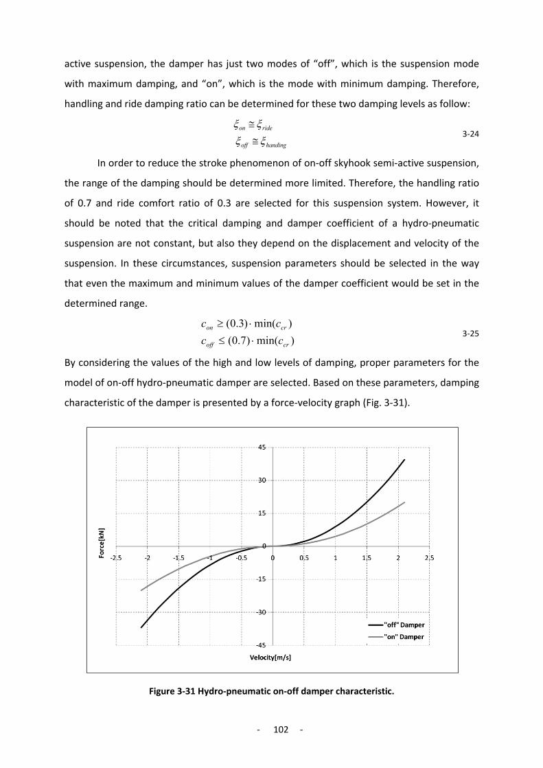
- 102 -

active suspension, the damper has just two modes of “off”, which is the suspension mode

with maximum damping, and “on”, which is the mode with minimum damping. Therefore,

handling and ride damping ratio can be determined for these two damping levels as follow:

handingoff

rideon

ξξξξ≅≅

3-24

In order to reduce the stroke phenomenon of on-off skyhook semi-active suspension,

the range of the damping should be determined more limited. Therefore, the handling ratio

of 0.7 and ride comfort ratio of 0.3 are selected for this suspension system. However, it

should be noted that the critical damping and damper coefficient of a hydro-pneumatic

suspension are not constant, but also they depend on the displacement and velocity of the

suspension. In these circumstances, suspension parameters should be selected in the way

that even the maximum and minimum values of the damper coefficient would be set in the

determined range.

)min()7.0()min()3.0(

croff

cron

cccc

⋅≤⋅≥

3-25

By considering the values of the high and low levels of damping, proper parameters for the

model of on-off hydro-pneumatic damper are selected. Based on these parameters, damping

characteristic of the damper is presented by a force-velocity graph (Fig. 3-31).

Figure 3-31 Hydro-pneumatic on-off damper characteristic.

- 103 -

As shown, the velocity-force curves of the hydro-pneumatic damper are not linear and rise in

a progressive way. It means that damper coefficient is not constant, but also it increases with

raising the damper velocity.

3.2.3 Cylinder Friction Model

In this section, the modeling of the friction effect in the hydro-pneumatic suspension

is considered. Friction is an unwanted effect in a suspension system and reduces its

performance. Similar to damping force, the friction force is always in the opposite direction

of the suspension movement. There are two kinds of frictions in a hydro-pneumatic

suspension.

The first kind of friction is created by the contact of oil with the inner area of other

components like pipe, cylinder, and throttle. This friction produces a pressure drop

proportional to the velocity of the suspension. Then, the cylinder converts this pressure to a

force similar to the damping force of the system. The example of this case is the friction

effect of the throttle that is the source of the damping force in a hydro-pneumatic

suspension. In this study, this kind of friction was also considered in the damper model.

Therefore, this kind of friction is considered as a useful effect, because it can be estimated in

the damping design of the system.

The second kind of friction is created by the contacts among the solid components of

a suspension, like the contact between a piston and the cylinder body or the contacts among

components of the mechanical mechanism of a suspension. This kind of friction is harmful,

because firstly, this friction is difficult to be calculated, and secondly, it is not proportional to

the suspension velocity and cannot be considered as the damping effect of the system.

Among these kinds of frictions, the static friction is particularly problematic, because it

appears at the beginning of the motion of the suspension, as no damping force is needed.

The cylinder is one component of a hydro-pneumatic suspension that produces this kind of

friction. This friction occurs because of the contact between the piston and cylinder body

through their sealing set (Fig. 3-32).

In order to consider the friction effect in the suspension model, in this section, the

model of the friction effect in the cylinders is built. For this purpose, the well-known friction

model of Coulomb is used. In this model, the friction force is independent of the slip velocity.

However, the friction coefficient with the slip velocity near zero is in practice higher (Fig 3-

- 104 -

33). This primary friction, calling as static friction, is more effective in suspension

performance, and it should be considered particularly in the friction model of the cylinder.

Figure 3-32 Hydraulic cylinder and relevant sealing components.

Figure 3-33 Relation of coulomb and static friction forces with the slip velocity of a hydraulic

cylinder.

Since coulomb and static friction are constant. The friction model of the cylinder is indeed a

switch that determines which one of these two friction forces adds to the cylinder force. The

mathematical model of the cylinder friction is defined as:

>−+≤−

=0)(0)(

vvFFvvF

Fcoulombstatic

staticf 3-26

In this formula, v is the symbol for the limit velocity of the static friction. Based on this

formulation, the Simulink model of the cylinder friction is built (Fig. 3-34).

Figure 3-34 Simulink model of the cylinder friction.

- 105 -

As mentioned, the coulomb friction force, static friction force, and static limit velocity

are constant values, and they are considered as the model parameters. In simulation, it was

supposed that the coulomb friction force of the hydro-pneumatic cylinder was negligible,

and the static friction force were determined via experimental measurement on the cylinder

of the prototype model. The Simulink model of the cylinder friction will be used in the model

of the hydro-pneumatic rear suspension presenting in the following section.

3.2.4 Overall Hydro-pneumatic Suspension Model

As was explained, in this investigation, the hydro-pneumatic rear suspension of the

tractor was equipped with a controllable damping system in order to be used as the actuator

for the semi-active suspension system. Figure 3.35 shows the circuit of the one unit of this

hydro-pneumatic suspension. For the modeling of this system, the hydro-pneumatic

suspension is divided into the two components: the hydro-pneumatic spring and the hydro-

pneumatic variable damper. The spring model consists of two components of the cylinder

and accumulator models, and variable damper consists of three components: throttle,

cylinder port, and valve models. Modeling of all these components was presented in the

previous sections. The final model of the actuator is created by joining all these components.

In this section, this model is presented.

Figure 3-35 Circuit of the one unit of the controllable hydro-pneumatic suspension used for the tractor rear suspension.

Figure 3-36 shows the final Simulink model of the hydro-pneumatic actuator unit,

which consists of four sub-models: cylinder, accumulator, throttling system, and cylinder

friction. Main component of this model is the cylinder model. This model receives the

displacement and the velocity of the suspension as the model inputs and delivers the

suspension force as the model output. By receiving the suspension input, the cylinder model

- 106 -

calculates the oil volume variation of both sides of the cylinder and sends these values to the

accumulator models.

Figure 3-36 Simulink model of the hydro-pneumatic actuator system.

On each side of the cylinder, the accumulator model calculates the created pressure

and sends it back to the cylinder model. This model can convert the received pressure to the

cylinder force. However, the effect of the throttle system on this pressure drop must be

considered before. For this purpose, the throttle model receives volumetric flow from the

cylinder model and based on the control command, determines the created pressure drop.

Now, total pressure of the cylinder can be calculated by subtracting this pressure drop from

the accumulator pressure. Based on this pressure, the cylinder model calculates the output

force. In the same time, the cylinder friction model calculates the friction force based on the

- 107 -

cylinder velocity. Therefore, the final suspension force is achieved by subtracting the friction

force from the cylinder force.

After building the hydro-pneumatic suspension model, this model can be applied to

the full tractor model. For this purpose, the simple linear model for the rear suspension units

is replaced by the hydro-pneumatic suspension model (Fig. 3-37).

Figure 3-37 Using of the model of the hydro-pneumatic suspension in the Simulink full tractor

model.

After this modeling, the last step is remained to complete the final simulation model.

This step is to create the controller model, and it will be presented in the following section.

3.3 Controller Model

The structure of the semi-active suspension system is illustrated in figure 3-38. This

structure consists of four components: tractor dynamics, actuator, sensors, and controller.

These components work all in a close loop. The controller monitors the dynamic behavior of

the tractor via the sensors. Then, based on the relevant control strategy, it produces the

control commands and sends them to the actuator in order to improve tractor dynamics.

In the previous sections, building the vehicle model and actuator model were

presented. Now in this section, modeling of the rest components of the system, namely

sensors and controller are considered. The sensors measure the vehicle dynamics

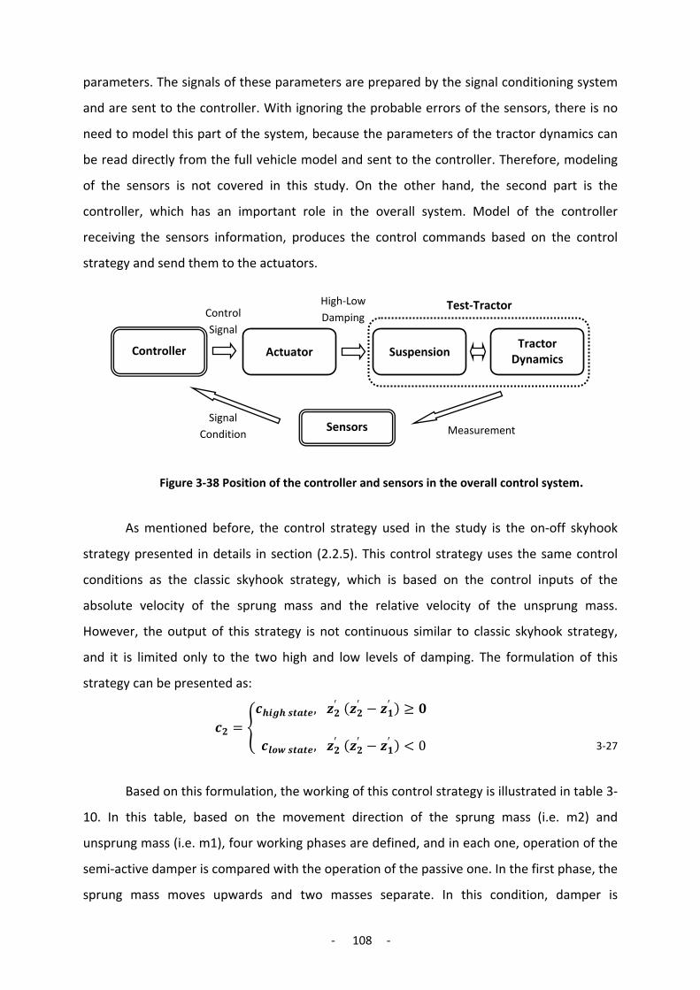
- 108 -

parameters. The signals of these parameters are prepared by the signal conditioning system

and are sent to the controller. With ignoring the probable errors of the sensors, there is no

need to model this part of the system, because the parameters of the tractor dynamics can

be read directly from the full vehicle model and sent to the controller. Therefore, modeling

of the sensors is not covered in this study. On the other hand, the second part is the

controller, which has an important role in the overall system. Model of the controller

receiving the sensors information, produces the control commands based on the control

strategy and send them to the actuators.

Figure 3-38 Position of the controller and sensors in the overall control system.

As mentioned before, the control strategy used in the study is the on-off skyhook

strategy presented in details in section (2.2.5). This control strategy uses the same control

conditions as the classic skyhook strategy, which is based on the control inputs of the

absolute velocity of the sprung mass and the relative velocity of the unsprung mass.

However, the output of this strategy is not continuous similar to classic skyhook strategy,

and it is limited only to the two high and low levels of damping. The formulation of this

strategy can be presented as:

𝒄𝒄𝟐𝟐 = �𝒄𝒄𝒉𝒉𝒉𝒉𝒉𝒉𝒉𝒉 𝒔𝒔𝒔𝒔𝒔𝒔𝒔𝒔𝒔𝒔, 𝒛𝒛𝟐𝟐′ (𝒛𝒛𝟐𝟐′ − 𝒛𝒛𝟏𝟏′ ) ≥ 𝟎𝟎

𝒄𝒄𝒍𝒍𝒍𝒍𝒍𝒍 𝒔𝒔𝒔𝒔𝒔𝒔𝒔𝒔𝒔𝒔, 𝒛𝒛𝟐𝟐′ (𝒛𝒛𝟐𝟐′ − 𝒛𝒛𝟏𝟏′ ) < 0� 3-27

Based on this formulation, the working of this control strategy is illustrated in table 3-

10. In this table, based on the movement direction of the sprung mass (i.e. m2) and

unsprung mass (i.e. m1), four working phases are defined, and in each one, operation of the

semi-active damper is compared with the operation of the passive one. In the first phase, the

sprung mass moves upwards and two masses separate. In this condition, damper is

Test-Tractor

Sensors

Controller Actuator Suspension Tractor

Dynamics

Measurement

Control Signal

Signal Condition

High-Low Damping

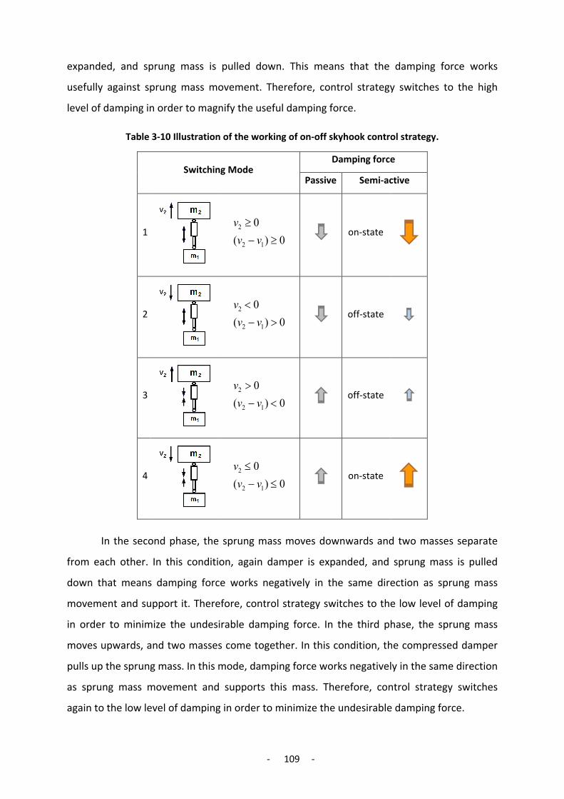
- 109 -

expanded, and sprung mass is pulled down. This means that the damping force works

usefully against sprung mass movement. Therefore, control strategy switches to the high

level of damping in order to magnify the useful damping force.

Table 3-10 Illustration of the working of on-off skyhook control strategy.

Damping force Switching Mode

Semi-active Passive

on-state

0)(0

12

2

≥−≥

vvv

1

off-state 0)(

0

12

2

>−<

vvv

2

off-state 0)(

0

12

2

<−>

vvv

3

on-state

0)(0

12

2

≤−≤

vvv

4

In the second phase, the sprung mass moves downwards and two masses separate

from each other. In this condition, again damper is expanded, and sprung mass is pulled

down that means damping force works negatively in the same direction as sprung mass

movement and support it. Therefore, control strategy switches to the low level of damping

in order to minimize the undesirable damping force. In the third phase, the sprung mass

moves upwards, and two masses come together. In this condition, the compressed damper

pulls up the sprung mass. In this mode, damping force works negatively in the same direction

as sprung mass movement and supports this mass. Therefore, control strategy switches

again to the low level of damping in order to minimize the undesirable damping force.

- 110 -

Finally, in the fourth phase, the sprung mass moves downwards, and two masses

come together. In this condition, the compressed damper pulls up the sprung mass. In this

mode, damping force works usefully against sprung mass movement. Therefore, control

strategy switches to the high level of damping in order to magnify the useful damping force.

To sum up, semi-active damper is tuned in the high level of damping, as damper force can be

useful for the damping of the sprung mass vibration. In opposition, semi-active damper is

tuned in the low damping level as the damper force is against damping of the sprung mass

vibration.

After the description of the control strategy, at this point, the method of applying the

control signals to the actuators should be determined. As mentioned before, the actuator of

each suspension unit is a double-acting cylinder with a throttle system on each side of it. As

experimental observations, it was found as the flowing oil toward the cylinder was throttled,

a vacuum effect was occurred in the cylinder, which was a disturbing phenomenon is hydro-

pneumatic suspension. On the other hand, this effect did not appear during the throttling of

the pressurized oil coming from the cylinder.

Therefore, as a design rule in this investigation, the high damping command of the

controller is applied to the throttle system of the just one side of the cylinder. It is the side

that oil is leaving the cylinder. The created damping level is the same as the determined

value, regardless of the cylinder side. Table 3-11 illustrates control commands in the four

control phases with respect to this rule. As shown, with the positive relative velocity, the

control command is applied to the throttle system of the rod side, and with the negative

relative velocity, the control command is applied to the throttle system of the head side.

Based on the table 3-11, the Simulink model of skyhook control strategy is built (Fig.

3-39). The inputs of this model are the absolute velocities of the sprung and unsprung

masses, and the outputs of the model are control commands, which are applied to both the

throttling systems of the head and rod sides of the cylinder. After building the controller

model, in order to examine its function, two sinusoidal waves were applied to the model as

the test input. Figure 3-40 shows the result of this test. The inputs waves and both rod and

piston cylinder control commands are shown in this chart. As shown, the outputs of the

model are created correctly based on the determined control approach.

- 111 -

Table 3-11 On-off skyhook control commands for the double-acting hydro-pneumatic cylinder.

Rod Side

Head Side

Damping State

Switching Mode

on off Hight 0)(

0

12

2

≥−≥

vvv

1

off off Low 0)(

0

12

2

>−<

vvv

2

off off Low 0)(

0

12

2

<−>

vvv

3

off on Hight 0)(

0

12

2

≤−≤

vvv

4

Figure 3-39 Simulink model of skyhook on-off controller for one suspension unit.

- 112 -

Figure 3-40 Control command for the rod and head cylinder sides using two sinusoidal waves as the input of control.

Figure 3-41 also shows how the controller model is joined to the full vehicle model.

Absolute velocities of the sprung mass and unsprung mass in the rear suspension units are

used as the input of the controller model. The outputs of the model are sent to the tractor

model. These outputs are the commands of the head and rod cylinder side of the tractor

model. The commands are applied to the models of the hydro-pneumatic rear suspension of

the tractor. This model is described in detail in section 3.2.4.

Figure 3-41 Connection of the Simulink control model to the full tractor model.

After the modeling of the controller and joining this model to the full tractor model,

the full tractor model is ready to be used for the simulation tests. However, the proper

design for the tests is needed and must be determined before. This subject will be presented

in chapter 5. In addition, the result of the simulation tests will be presented in chapter 6.

However, before presenting these chapters, the prototype phase of this study will be

presented in the following chapter.

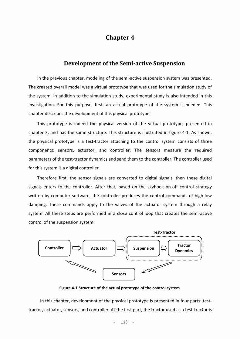
- 113 -

Chapter 4

4 Development of the Semi-active Suspension

In the previous chapter, modeling of the semi-active suspension system was presented.

The created overall model was a virtual prototype that was used for the simulation study of

the system. In addition to the simulation study, experimental study is also intended in this

investigation. For this purpose, first, an actual prototype of the system is needed. This

chapter describes the development of this physical prototype.

This prototype is indeed the physical version of the virtual prototype, presented in

chapter 3, and has the same structure. This structure is illustrated in figure 4-1. As shown,

the physical prototype is a test-tractor attaching to the control system consists of three

components: sensors, actuator, and controller. The sensors measure the required

parameters of the test-tractor dynamics and send them to the controller. The controller used

for this system is a digital controller.

Therefore first, the sensor signals are converted to digital signals, then these digital

signals enters to the controller. After that, based on the skyhook on-off control strategy

written by computer software, the controller produces the control commands of high-low

damping. These commands apply to the valves of the actuator system through a relay

system. All these steps are performed in a close control loop that creates the semi-active

control of the suspension system.

Figure 4-1 Structure of the actual prototype of the control system.

In this chapter, development of the physical prototype is presented in four parts: test-

tractor, actuator, sensors, and controller. At the first part, the tractor used as a test-tractor is

Test-Tractor

Sensors

Controller Actuator Suspension Tractor

Dynamics

- 114 -

introduced. Then, building the actuator system that is the hydro-pneumatic rear suspension

of the test-tractor with a controllable damping system is presented. After that, the sensors

of the control system and installation of them on the test-tractor are explained. At the end,

development of the hardware and the software parts of the controller is described.

4.1 Test-Tractor

A semi-active controller prototype cannot be evaluated by itself. It can be evaluated,

when the semi-active controller is applied to the suspension of a tractor, and the influence

of this system on the dynamics of the tractor is measured. Therefore, as the first step of

prototype developing, a tractor was determined as the test-tractor of the system. As stated

in section 2.6.6, the test-tractor used for this investigation was TUB-Trac (Fig. 4-2).

This tractor was indeed MB-1600 tractor that was converted to a full suspension

tractor by attaching a hydro-pneumatic suspension on the rear axle. This work was

performed before at the TU Berlin - Department Machinery System Design as a research

project, and after that, it is called TUB-Trac and used for research works in suspension area

as a test-tractor. Figure 4-2 shows this tractor and relevant rear and front axle suspensions.

Figure 4-2 Test-tractor with the conventional suspension of the front axle and the hydro-pneumatic suspension of the rear axle.

This tractor is a full suspension tractor with a hydro-pneumatic suspension for the

rear axle. A full suspension system is considered as the most complete passive suspensions

for a tractor. As the next step, the application of an active suspension is defined. This

provides better suspension performance, which is the objective of this investigation. On the

other hand, the hydro-pneumatic suspension can be converted simply to an active

suspension system. This is possible because of the simplification in building the actuation

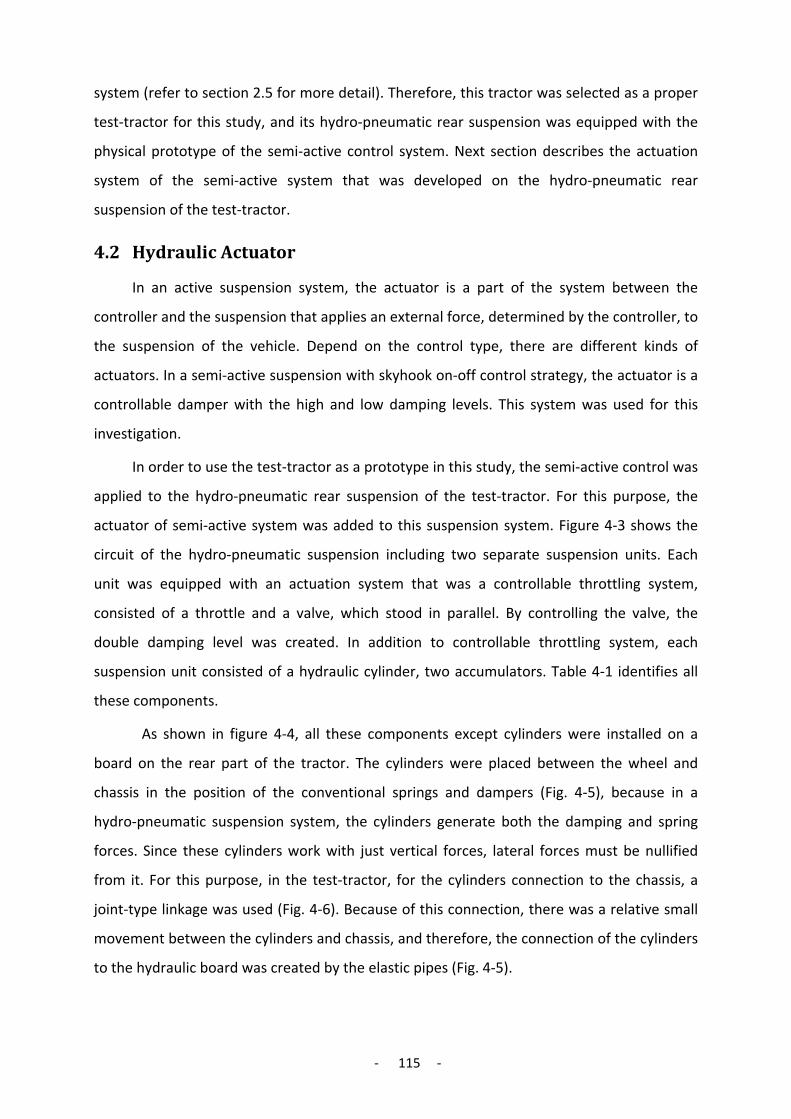
- 115 -

system (refer to section 2.5 for more detail). Therefore, this tractor was selected as a proper

test-tractor for this study, and its hydro-pneumatic rear suspension was equipped with the

physical prototype of the semi-active control system. Next section describes the actuation

system of the semi-active system that was developed on the hydro-pneumatic rear

suspension of the test-tractor.

4.2 Hydraulic Actuator

In an active suspension system, the actuator is a part of the system between the

controller and the suspension that applies an external force, determined by the controller, to

the suspension of the vehicle. Depend on the control type, there are different kinds of

actuators. In a semi-active suspension with skyhook on-off control strategy, the actuator is a

controllable damper with the high and low damping levels. This system was used for this

investigation.

In order to use the test-tractor as a prototype in this study, the semi-active control was

applied to the hydro-pneumatic rear suspension of the test-tractor. For this purpose, the

actuator of semi-active system was added to this suspension system. Figure 4-3 shows the

circuit of the hydro-pneumatic suspension including two separate suspension units. Each

unit was equipped with an actuation system that was a controllable throttling system,

consisted of a throttle and a valve, which stood in parallel. By controlling the valve, the

double damping level was created. In addition to controllable throttling system, each

suspension unit consisted of a hydraulic cylinder, two accumulators. Table 4-1 identifies all

these components.

As shown in figure 4-4, all these components except cylinders were installed on a

board on the rear part of the tractor. The cylinders were placed between the wheel and

chassis in the position of the conventional springs and dampers (Fig. 4-5), because in a

hydro-pneumatic suspension system, the cylinders generate both the damping and spring

forces. Since these cylinders work with just vertical forces, lateral forces must be nullified

from it. For this purpose, in the test-tractor, for the cylinders connection to the chassis, a

joint-type linkage was used (Fig. 4-6). Because of this connection, there was a relative small

movement between the cylinders and chassis, and therefore, the connection of the cylinders

to the hydraulic board was created by the elastic pipes (Fig. 4-5).

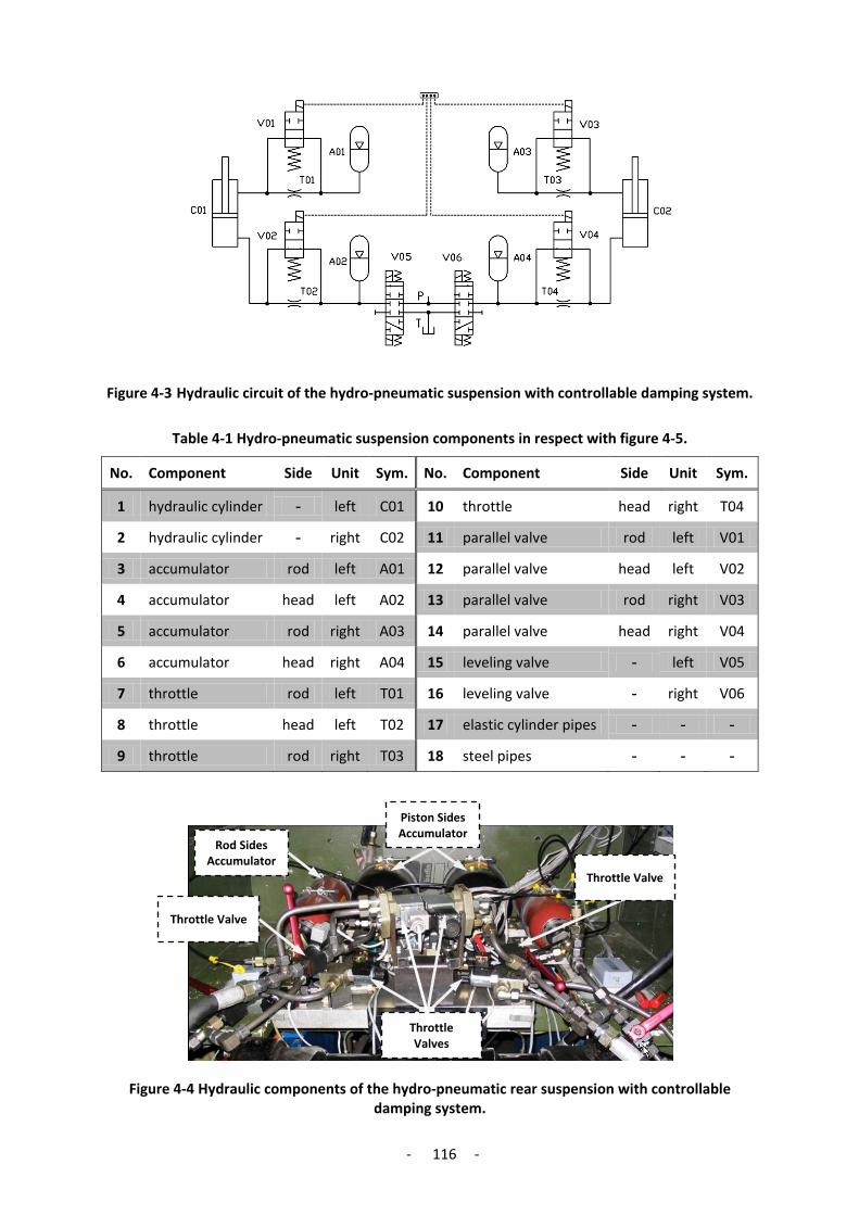
- 116 -

Figure 4-3 Hydraulic circuit of the hydro-pneumatic suspension with controllable damping system.

Table 4-1 Hydro-pneumatic suspension components in respect with figure 4-5.

No. Component Side Unit Sym. No. Component Side Unit Sym.

1 hydraulic cylinder - left C01 10 throttle head right T04

2 hydraulic cylinder - right C02 11 parallel valve rod left V01

3 accumulator rod left A01 12 parallel valve head left V02

4 accumulator head left A02 13 parallel valve rod right V03

5 accumulator rod right A03 14 parallel valve head right V04

6 accumulator head right A04 15 leveling valve - left V05

7 throttle rod left T01 16 leveling valve - right V06

8 throttle head left T02 17 elastic cylinder pipes - - -

9 throttle rod right T03 18 steel pipes - - -

Figure 4-4 Hydraulic components of the hydro-pneumatic rear suspension with controllable damping system.

Piston Sides Accumulator

Rod Sides Accumulator

Throttle Valves

Throttle Valve

Throttle Valve

- 117 -

Figure 4-5 Position of the hydraulic cylinder in the rear axle suspension of the tractor.

These cylinders were specialized hydro-pneumatic suspension cylinders, which were

equipped with a special seal system in order to provide a low friction level. The cylinders

used for rear axle suspension were double-acting type providing the feasibility of controlling

on both sides of the cylinder. Likewise, in this investigation, the throttling system was

applied to both sides of the cylinder.

Another point about the cylinders is the throttling effect of their ports. As stated

chapter 3, this throttling effect was considered in the design calculation of the damper for

the system as the only throttling effect of the system in the mode of low-level damping.

Figure 4-6 shows these cylinder ports. The detailed specification of the cylinder such as the

piston area, ports cross-section, and friction force are presented along with simulation

parameters in appendix E4.

Specific property of the hydro-pneumatic suspension that was used for this study was

the control ability of the damping level of the suspension. This ability was created in the

prototype by mean of a special throttling system comprised of a throttle and a parallel valve

(Fig. 4-4 and Fig. 4-7). Working of this system was described in section 3.2.2. The throttle

used in the system was an adjustable throttle-valve providing the high damping level and

passive damping level for the suspension. This valve also provided the possibility of testing of

other damping levels for these two damping modes. Determination of the proper value for

these two damping levels was described in section 3.2.6.

The valves, standing in parallel with the throttles, were the only controllable

elements of the system that provide the ability of controlling the damping level of the

Hydraulic Cylinder

Elastic Hydraulic

Pipe

Hydraulic board

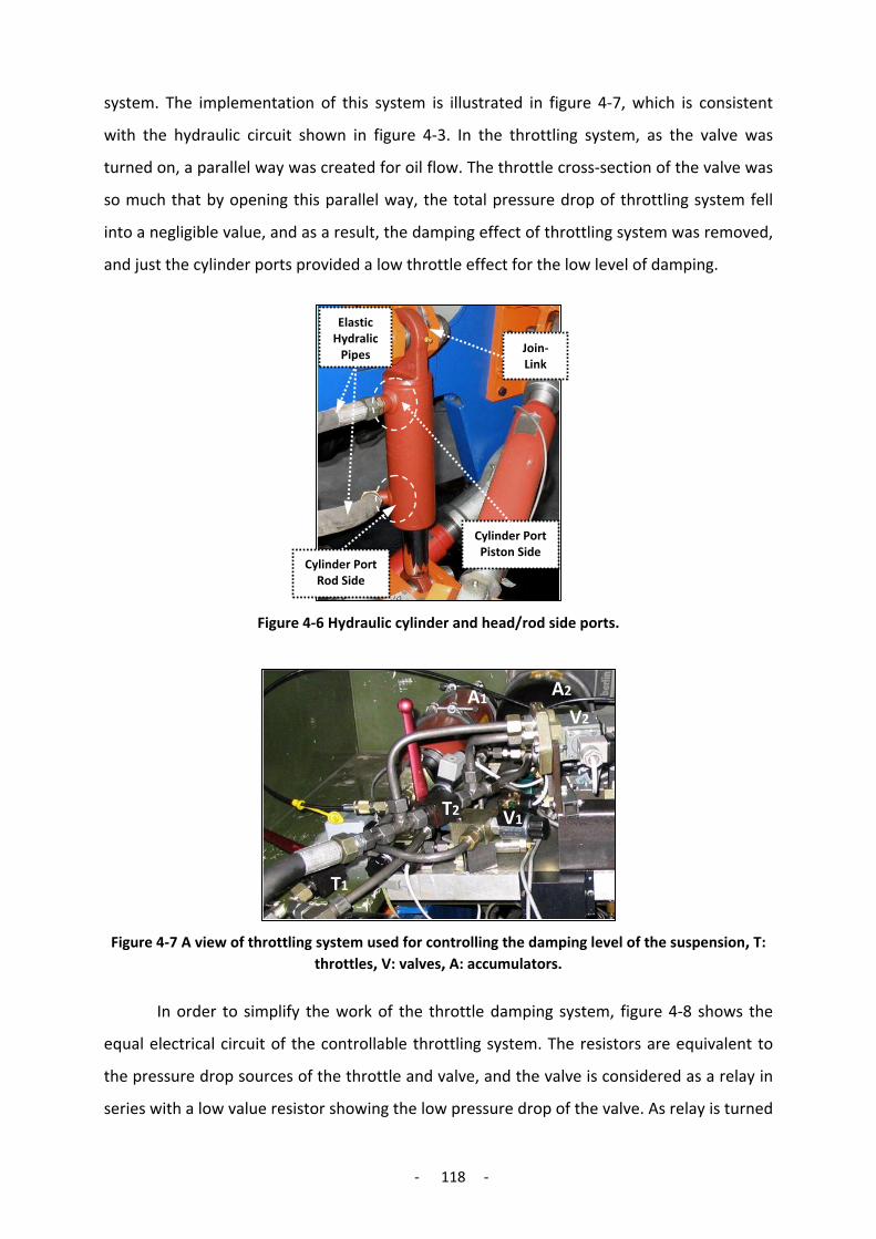
- 118 -

system. The implementation of this system is illustrated in figure 4-7, which is consistent

with the hydraulic circuit shown in figure 4-3. In the throttling system, as the valve was

turned on, a parallel way was created for oil flow. The throttle cross-section of the valve was

so much that by opening this parallel way, the total pressure drop of throttling system fell

into a negligible value, and as a result, the damping effect of throttling system was removed,

and just the cylinder ports provided a low throttle effect for the low level of damping.

Figure 4-6 Hydraulic cylinder and head/rod side ports.

Figure 4-7 A view of throttling system used for controlling the damping level of the suspension, T:

throttles, V: valves, A: accumulators.

In order to simplify the work of the throttle damping system, figure 4-8 shows the

equal electrical circuit of the controllable throttling system. The resistors are equivalent to

the pressure drop sources of the throttle and valve, and the valve is considered as a relay in

series with a low value resistor showing the low pressure drop of the valve. As relay is turned

Join-Link

Elastic Hydralic

Pipes

Cylinder Port Piston Side

Cylinder Port Rod Side

T1

T2

V2

V1

A2 A1

- 119 -

on, the low value resistor stands in parallel to the high value resistor of the throttle. This

decreases completely the total resistance, so that just the resistor of the cylinder port stays

in the circuit.

Figure 4-8 Throttle damping system with equivalent electrical circuit.

As a result, the calculation of total pressure drop for two damping levels can be

derived from the equal electric circuit as follow:

portvalvethrottle

valvethrottleporttotal

throttleporttotal

PPPPPPPModeLow

PPPModeHigh

∆≅∆+∆∆⋅∆

+∆=∆

∆+∆=∆

,""

,"" 4-1

Therefore, for selecting the valves, there was no need to calculate the quantity of

their throttling effect and just the throttle cross-section of the valve had to be in a size that

the total pressure drop would be negligible. With this design, the throttling effect of this part

of the system was removed. The characteristic curves of the 2-way solenoid valves used for

controllable throttling system, was derived from relevant hydraulic handbooks. These curves

indicate the relation between the pressure drop and flow rate of the valves and were used in

order to determine the throttling effect of the valves in different flow rates. This was done to

ensure that in the mode of low damping, the throttling effect of the parallel throttle set was

negligible. In other words, the parallel throttle set was equal to a piece of hydraulic pipe

connection in this mode.

In addition to throttle electro-vales, there are two other directional solenoid valves in

the hydraulic circuit (V05 and V06 in figure 4-3). These valves were used by auto leveling

control system as an actuation system to adjust the suspension height of the tractor. These

- 120 -

valves were used in a way that by receiving the control commands, the head side of the

cylinder was connected to the pressurized oil. This filled the cylinder and increased the

suspension height. On the other hand, in order to decrease the suspension height, the

cylinders were discharged by connecting to the oil tank via the valves. More detail about

load leveling will be given in section 4.5.2.

Another component of a hydro-pneumatic suspension is the accumulator, which

creates the spring force of the system. The accumulators used for the system were bladder-

type, which provides a good dynamic response in hydro-pneumatic suspension (refer to Fig.

4-4 and 4-7). Volume capacity of the accumulators was selected so that to cover the

maximum volume of the cylinder. Moreover, the pre-charge gas pressures of the

accumulators were adjusted by adding pressurized nitrogen gas with respect to the

determined values mentioned in appendix E4. At this point, after the description of

actuation system, the controller components of the prototype will be explained in the

following sections.

4.3 Velocity Sensors

In order to find the require sensors for the semi-active suspension system, it should be

referred to Section 3.3 that describes skyhook on-off control strategy used for the semi-

active suspension. Looking at table 3-11, the needed parameters can be identified that are

the absolute velocity of the tractor body (i.e. sprung mass) and the relative velocity between

the tractor body and wheel (i.e. unsprung mass). On the prototype, each unit of the semi-

active suspension was considered independent and, in order to measure the velocity of the

sprung mass (m2), the velocity of the corners of the tractor body was measured (Fig 4-9).

Moreover, in order to measure the velocity of the unsprung mass (m1), the velocity of the

corners of the rear axle was measured.

Figure 4-9 Using velocity sensors for the on-off semi-active control on the rear axle suspension.

- 121 -

One technique used for measuring the absolute velocity is to derive it from the

absolute accelerometer signals. For this purpose, the absolute acceleration of the tractor

body is measured by an accelerometer. Then, accelerometer signals are integrated in order

to achieve the corresponding velocity signals. The integration could be performed either

digitally by a computer or in analog by an integrator circuit. However, because of the

necessary signal integrating, this method is considered as a difficult method and associated

with errors.

In this investigation, the experimental tests were performed on a suspension test rig,

and it was not needed to move the tractor during the tests. Therefore, it was possible to

measure the absolute velocity directly by velocity sensors. For this purpose, a cable-type of

velocity transducers was used in order to measure the absolute velocity of the tractor body.

This sensor was fixed on the ground, and then, cable of the sensor was fixed to the directly

upside point of the tractor body (Fig. 4-9).

In order to measure the relative velocity between the tractor body and wheel, again,

a cable-type of velocity transducers was installed on the tractor mudguard, and then, the

cable was fixed to the directly downside point of the wheel (Fig. 4-9). Technical data of this

transducer is presented in appendix C2. The velocity signal of this transducer was out of

noise, linear and self-energizing. In this way, a proper signal for the control system was

provided. In spite of this, in order to remove the effect of the high frequency vibrations on

the vibrations signal, an external low pass filter with the cut-off frequency of 25 Hz was used.

This filtered the transducers signals before applying them to the controller.

4.4 Controller Hardware Development of the components of the control system including test-tractor,

actuator, and sensors were described in the previous section. At this point, development of

the controller is explained. Figure 4-10 illustrates the structure of the used controller for this

investigation. This controller was indeed a personal computer with control software that was

connected to the control input-output via an interface card.

As the input of control, the analog signals of the velocity transducers were applied to

the interface card, while this interface card worked just with digital signals. Therefore, an

ADC circuit was used in order to covert the analog signals to the digital ones before entering

to the interface card. On the other hand, the interface card was not able to drive the

solenoid valves directly. Though the digital output signal of the interface card was matched

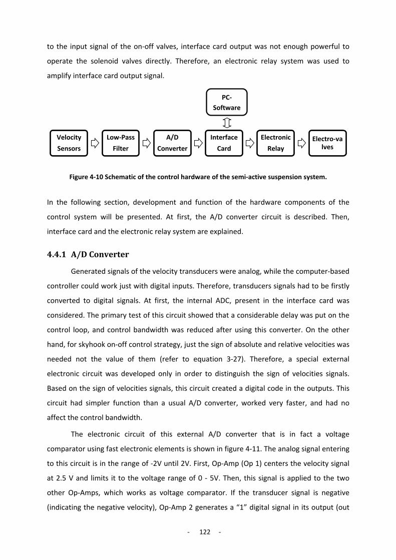
- 122 -

to the input signal of the on-off valves, interface card output was not enough powerful to

operate the solenoid valves directly. Therefore, an electronic relay system was used to

amplify interface card output signal.

Figure 4-10 Schematic of the control hardware of the semi-active suspension system.

In the following section, development and function of the hardware components of the

control system will be presented. At first, the A/D converter circuit is described. Then,

interface card and the electronic relay system are explained.

4.4.1 A/D Converter

Generated signals of the velocity transducers were analog, while the computer-based

controller could work just with digital inputs. Therefore, transducers signals had to be firstly

converted to digital signals. At first, the internal ADC, present in the interface card was

considered. The primary test of this circuit showed that a considerable delay was put on the

control loop, and control bandwidth was reduced after using this converter. On the other

hand, for skyhook on-off control strategy, just the sign of absolute and relative velocities was

needed not the value of them (refer to equation 3-27). Therefore, a special external

electronic circuit was developed only in order to distinguish the sign of velocities signals.

Based on the sign of velocities signals, this circuit created a digital code in the outputs. This

circuit had simpler function than a usual A/D converter, worked very faster, and had no

affect the control bandwidth.

The electronic circuit of this external A/D converter that is in fact a voltage

comparator using fast electronic elements is shown in figure 4-11. The analog signal entering

to this circuit is in the range of -2V until 2V. First, Op-Amp (Op 1) centers the velocity signal

at 2.5 V and limits it to the voltage range of 0 - 5V. Then, this signal is applied to the two

other Op-Amps, which works as voltage comparator. If the transducer signal is negative

(indicating the negative velocity), Op-Amp 2 generates a “1” digital signal in its output (out

Velocity

Sensors

Low-Pass

Filter

A/D

Converter

Interface

Card

Electronic

RelayElectro-va

lves

PC-Software

- 123 -

1), and if the transducer signal is positive, which indicated the positive velocity, Op-Amp 3

generates a “1” digital signal in its output (out 2). Figure 4-12 shows the output of the circuit

for a sinusoidal wave input.

Figure 4-11 Electronic circuit of a ADC unit.

Figure 4-12 Digital output of the ADC circuit, entering a sinusoidal wave input.

Such an ADC circuit was used for each velocity transducer signal. Therefore, the four

units of this circuit were used for the four velocities signals coming from the velocities

sensors of the system. The output digital signal was fitting to the input of the interface card,

and it could be applied directly.

4.4.2 Interface Card

The digital controller in this investigation was a personal computer that was

communicated to the inputs and outputs of control via an interface card. The interface card

used for this investigation was a data acquisition card (NI-DAQ) from National Instruments,

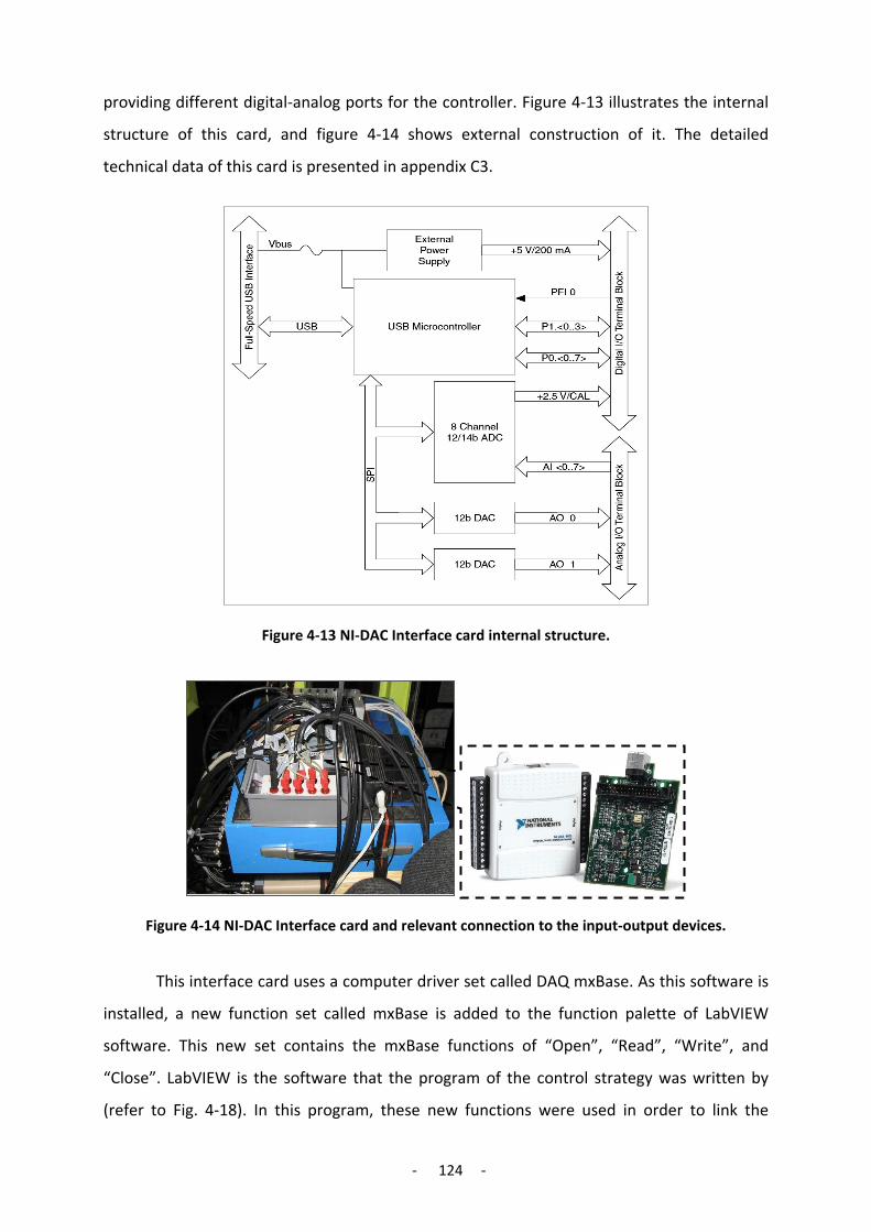
- 124 -

providing different digital-analog ports for the controller. Figure 4-13 illustrates the internal

structure of this card, and figure 4-14 shows external construction of it. The detailed

technical data of this card is presented in appendix C3.

Figure 4-13 NI-DAC Interface card internal structure.

Figure 4-14 NI-DAC Interface card and relevant connection to the input-output devices.

This interface card uses a computer driver set called DAQ mxBase. As this software is

installed, a new function set called mxBase is added to the function palette of LabVIEW

software. This new set contains the mxBase functions of “Open”, “Read”, “Write”, and

“Close”. LabVIEW is the software that the program of the control strategy was written by

(refer to Fig. 4-18). In this program, these new functions were used in order to link the

- 125 -

controller program to the inputs and outputs of the card, which were indeed the control

inputs, and outputs.

As shown in figure 4-13, the core of this interface card is a controller that

communicates with the computer through a USB port and provides the digital inputs and

outputs for the computer. Besides this controller, there are A/D and D/A converters. By

these converters, the card can receive the analog inputs and create analog outputs.

However, they were not used in the suspension controller, because the bandwidth of the

card would be decreased until 10 kHz after using these converters, and the controller

bandwidth would be reduced largely. Therefore, instead of the internal ADC, an external ADC

was developed and used for converting the control inputs. This external converter was

described in the previous section. By using the external converter, just the digital ports of

the interface card were used. This led that interface card worked with high sampling rate, so

that, the effect of card delay in control bandwidth was negligible.

The interface card was placed in the driver cabin beside other electronic components

so that it could be connected directly to the input-output of the devices (refer to Fig. 5-20).

Since the computer was placed out of the tractor, its communication with the interface card

was made by means of a long USB cable.

4.4.3 Electronic Relay System

Control output signals from the interface card were not enough powerful so as to be

applied directly to the solenoid valves. Therefore, this output signals were amplified firstly by

a relay system. Since the conventional electro-mechanic relays are not enough fast for the

control system, an electronic relay circuit was applied. Figure 4-15 shows the circuit of the

one unit of the electronic relay system.

Figure 4-15 The electronic relay circuit used for driving the solenoid valves of the actuators.

- 126 -

In this circuit, the output signal of the interface card passes through the opto-coupler

to an amplifier. Then, output of this amplifier put into the “base” connection of a power

transistor in order to turn the transistor on. This power transistor works as a switch in this

circuit and could afford until 5 amperes, which was enough for switching the solenoid valves.

Using an opto-coupler in this circuit provided a complete isolation between the valve circuit

and control circuit that protected interface card ports. In addition, a diode connecting to the

output of the circuit protected the power transistor from the high voltage signals, which

come from the solenoid valve as it was turning off. This occurred because of an inductance

effect in the valve’s solenoids.

In the practice circuit, each unit of the relay circuits was placed in a red capsule.

Figure 4-16 shows the developed electronic relay system including 10 relay channels, which

were enough in order to cover all the output channels of the system. Table 4-2 presents the

technical data of these electronic relay units.

Figure 4-16 Developed electronic relay system.

Table 4-2 Technical data of the electronic relay system.

Control Circuit (Input) Load Circuit (Output)

Voltage 3-24 V Voltage 3-60 V-DC

Current Max. 24 mA by 24V Current 0.01-3A, shock current: 5A 1s

4.5 Controller Software

In this investigation, a personal computer was used as the controller of the system.

This computer was connected to an I/O card in order to communicate with the output and

input of the control. Using special software, this computer was able to execute the strategy

of control. The controller read the inputs and generated a command based on the control

Electronic Relay Unit

- 127 -

strategy to put into the actuator. Then, the three main components of the control system

were; input, output, and the control strategy. The inputs of control were the transducers

signals of the absolute velocity of the tractor body and the relative velocities between the

wheels and body of the tractor. Moreover, the outputs of the controller were switching

signals, which were applied to the valves of both sides of the hydraulic cylinders. The third

part is the control strategy of the semi-active suspension control, which was the skyhook on-

off control strategy in this study. The input and output devices of the control system were

presented in the previous sections.

The software of the controller performs the control strategy. In this section, this

software is described. The flowchart of the control strategy is illustrated in figure 4-17. This

flowchart is created based on the description of the control strategy, which was presented in

detail in section 3.3.

Figure 4-17 Flowchart of skyhook on-off control strategy.

No

Yes

Yes

No

Turn on the electro-valve

of rod-side

Yes

No

Start on-off skyhook strategy

End on-off skyhook strategy

Turn on the electro-valve

of piston-side

Is relative velocity

negative?

Is relative velocity

negative?

Is body velocity

negative?

Turn off the electro-valves

- 128 -

The computer programming for the controller was done in LabVIEW software, which

is a graphical programming language from National Instruments used for writing the

instrumentation programs. This software was used for the controller, because it was

matched completely with the NI-DAQ interface card, recommended by the card

manufacturer. As mentioned, this card was driven by software called DAQ mxBase. As this

software was installed, a new function set was added to LabVIEW software. This provided an

access to the input and output ports of the interface card, which were equal to the inputs

and outputs of the control.

Figure 4-18 shows a screen captured from the diagram of the controller program,

which was a LabVIEW program. This program consisted of two similar controller units, which

were used for the right and left suspension units of the rear axle suspension. Each controller

unit was made of the three parts: input, control logic, and output.

Figure 4-18 Block Diagram of the LabVIEW program of the semi-active controller.

The control inputs were the converted digital signals from the velocity transducers

signals producing by A/D circuit. In this circuit, there were two digital outputs for each

velocity sensor, which were applied to the two digital input ports of the I/O card. These

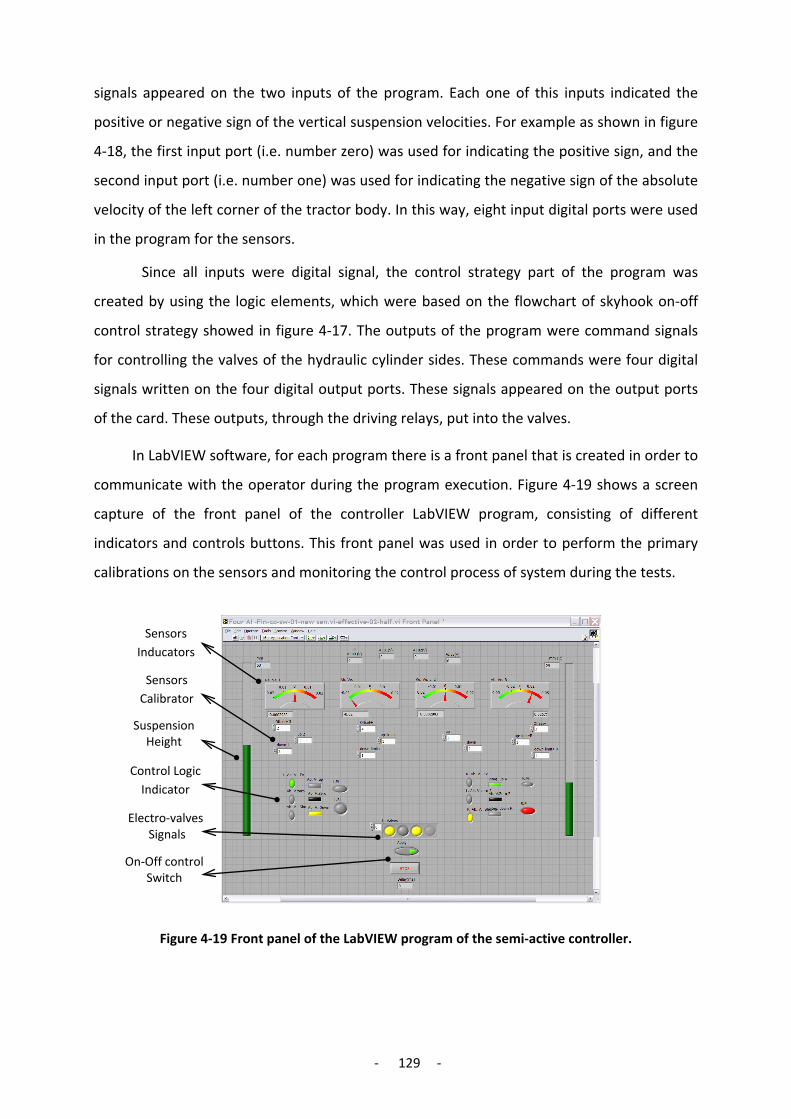
- 129 -

signals appeared on the two inputs of the program. Each one of this inputs indicated the

positive or negative sign of the vertical suspension velocities. For example as shown in figure

4-18, the first input port (i.e. number zero) was used for indicating the positive sign, and the

second input port (i.e. number one) was used for indicating the negative sign of the absolute

velocity of the left corner of the tractor body. In this way, eight input digital ports were used

in the program for the sensors.

Since all inputs were digital signal, the control strategy part of the program was

created by using the logic elements, which were based on the flowchart of skyhook on-off

control strategy showed in figure 4-17. The outputs of the program were command signals

for controlling the valves of the hydraulic cylinder sides. These commands were four digital

signals written on the four digital output ports. These signals appeared on the output ports

of the card. These outputs, through the driving relays, put into the valves.

In LabVIEW software, for each program there is a front panel that is created in order to

communicate with the operator during the program execution. Figure 4-19 shows a screen

capture of the front panel of the controller LabVIEW program, consisting of different

indicators and controls buttons. This front panel was used in order to perform the primary

calibrations on the sensors and monitoring the control process of system during the tests.

Figure 4-19 Front panel of the LabVIEW program of the semi-active controller.

Sensors Inducators

Electro-valves Signals

Sensors Calibrator

Control Logic Indicator

On-Off control Switch

Suspension Height

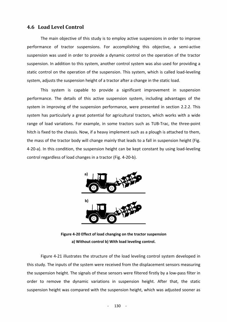
- 130 -

4.6 Load Level Control

The main objective of this study is to employ active suspensions in order to improve

performance of tractor suspensions. For accomplishing this objective, a semi-active

suspension was used in order to provide a dynamic control on the operation of the tractor

suspension. In addition to this system, another control system was also used for providing a

static control on the operation of the suspension. This system, which is called load-leveling

system, adjusts the suspension height of a tractor after a change in the static load.

This system is capable to provide a significant improvement in suspension

performance. The details of this active suspension system, including advantages of the

system in improving of the suspension performance, were presented in section 2.2.2. This

system has particularly a great potential for agricultural tractors, which works with a wide

range of load variations. For example, in some tractors such as TUB-Trac, the three-point

hitch is fixed to the chassis. Now, if a heavy implement such as a plough is attached to them,

the mass of the tractor body will change mainly that leads to a fall in suspension height (Fig.

4-20-a). In this condition, the suspension height can be kept constant by using load-leveling

control regardless of load changes in a tractor (Fig. 4-20-b).

Figure 4-20 Effect of load changing on the tractor suspension

a) Without control b) With load leveling control.

Figure 4-21 illustrates the structure of the load leveling control system developed in

this study. The inputs of the system were received from the displacement sensors measuring

the suspension height. The signals of these sensors were filtered firstly by a low-pass filter in

order to remove the dynamic variations in suspension height. After that, the static

suspension height was compared with the suspension height, which was adjusted sooner as

a)

b)

- 131 -

the desired primary height. If the static height changing occurred, and it continued for a

specific period, the system recognized it as a static change in suspension height and sent

proper output signals to the actuator in order to change the suspension height into the

primary value.

Figure 4-21 Block diagram of the load leveling control system.

For load leveling control system, a hardware configuration similar to the semi-active

suspension control was used. In figure 4-22, the configuration of this system is shown. The

controller of the system was the same computer as the semi-active controller with a new

interface card and separate control software. Since the bandwidth of the load-leveling

controller was largely lower than the bandwidth of the semi-active controller, the priority in

computer response was set on the semi-active control over the load leveling control, so no

interrupt occurred in operation of the semi-active controller.

Figure 4-22 Block diagram of the load leveling control system.

The program of the load-leveling controller was created in LabVIEW software. In this

software, instead of the external ADC circuit controller, the internal ADC component of the

interface card was used, and low-pass filter were performed by controller software. This led

to increase the delay of the controller loop. Since a low bandwidth control was needed for

this system, the delays created by these components did not disturb the system.

Distance Sensors

Low-Pass Filter

Height Comparison Timer

Electronic

Relay

Electro-

valves

Displacement

Sensors

Interface

Card

Electronic

Relay

Pressure

Electrovalves

Desire Height

Sensitivity Controller

PC

- 132 -

Figure 4-23 illustrates the block diagram of this program that consists of six parts:

input, low-pass filter, comparator I, timer, comparator II, and output. The first part includes

two A/D converters to convert the analog signals of the displacement sensors to digital

signals. These sensors were used for measurement of the suspension height. The second

part is a low-pass filter with the cut-off frequency of 0.1 Hz, which was used to remove the

signals of the dynamic change in suspension height. The third part is a comparator that lets

the operator determines the primary height of the suspension. In addition, the sensitivity of

the controller in responding to the static change in suspension height could be adjustable in

this part.

Figure 4-23 Block diagram of LabVIEW program of the load leveling controller.

The forth part of the software is a timer that was used in order to measure the

duration of static changes in suspension height to ensure that the change was not just a

Low Pass Filter

Output

Timer

Input

Comparator I Comparator II

- 133 -

transient one. The fifth part after receiving the output signal of the timer, created the proper

commands into the valves with the intention of running the cylinders so as to correct the

suspension height. This part compared continuously the suspension height with primary

height. This caused that the cylinders kept running until the height was corrected. The sixth

part is the output part that sent the control commands to the output of the interface card.

The hydraulic circuit of the hydro-pneumatic suspension for the rear axle was

presented in section 4.2 in figure 4-3. The directional solenoid valves that received these

commands were the valves number 5 and 6 in this circuit. As the suspension height should

be increased, the hydraulic oil was pressurized to the head side of the cylinder via these

valves. On the contrary, the initial pressure of the head side of the cylinder was decreased by

directing the oil to the tank as the suspension height should be decreased.

In semi-active control, a cable-type of velocity transducers was used to measure the

relative velocity of the suspension. These sensors can measure the displacement as well

(appendix C2). The displacement signals of these sensors were used as the input of the load-

leveling controller.

As the load leveling control system works with a very low frequency, evaluation of

this system was performed by applying an extra load to the system. Then, it was observed if

the reaction of the control system was correct and the tractor body became again level after

the delay time. These tests showed the correct operation of the system.

In chapter 4, development of the prototype of the full suspension tractor was

described. This prototype contained the semi-active and load leveling control system on the

rear axle suspension. In the next chapter, the test setup, which was indeed the preparation

for the evaluation system tests, will be presented.

- 134 -

Chapter 5

5 Simulation and Experimental Test

After building the computer model and developing the virtual prototype, the

simulation and experimental tests can be performed. However, the tests should be designed,

and their details should be determined before. In this chapter, the design and performance

of the simulation tests and experimental tests are described.

5.1 Test Design

An objective of this investigation is the evaluation of the new suspension system. To

begin with accomplishing the evaluation, a proper test design should be determined.

General steps of the tests are illustrated in figure 5-1. The first step was the application of

the test input to the test-tractor in order to excite the suspension system. In the second

step, by preparing the system and applying the test input to the system, the test was

performed. As the third step, the outcomes of the tests, which were the time history curves

of the output parameters, were read as the test output. This data was saved by a data logger

to use them later for the final step, which was the data analysis. By analyzing the data, the

results of the tests are concluded.

Figure 5-1 Process of the test implementation.

The test design and test plan will be described in the following sections. First, the

test-output are determined. These outputs are the parameters that evaluation criteria of the

system are inferred from them. Then, the data reduction methods are explained. After that,

test-input used for suspension excitation is described. Finally, all these cases of the test

design are considered for making the plan of the tests.

Test Input Test Running Test Output Data

Analysis

- 135 -

5.1.1 Test Output

In order to design a test, the output of the test should be determined initially. The

output of a test depends on the goal of the performing the test. In this study, the goal was to

evaluate the performance of the new suspension system. Therefore, the criteria of a

suspension performance should be determined initially. These criteria were considered the

ride comfort and vehicle handling of the tractor. The definition and importance of these

factors were stated in section 2.1.1 and 2.1.2 .

Ride comfort, implying the comfort of the driver, depends on the vibration of the

tractor body. Therefore, the accelerations of the tractor body including “Heave”, ”Pitch”, and

“Roll” accelerations were measured. Vehicle handling, involving vehicle stability and safety,

depends on the road contact of the tires, which is affected by the tractor body and wheel

vibrations. This parameter is evaluated by measuring the vertical dynamic force of the tire

contact called in short form “dynamic tire force”. Besides the two parameters, another

parameter is considered. This parameter is maximum suspension travel, which is related to

the constructional design of a suspension system and indicates the required suspension

stroke in the design of the suspension.

5.1.2 Data Reduction

From the evaluation tests, two groups of the time-domain and frequency-domain

results were achieved. In order to perform the vibration analysis of the new suspension,

these results should be studied. For this purpose, the two main analysis method of

amplitude-based and frequency-based were used for the test data reduction, which will be

described in the following sections.

5.1.2.1 Amplitude-Based Analysis

Amplitude-based analysis is used normally for the data reduction purpose in order to

derive a quantity indicating the magnitude characteristic of a data series. The most used

expressions for the amplitude of a set of data is root-mean-square that is often abbreviated

as “RMS”. This quantitative parameter, presenting the average of data magnitudes is used

for the analysis of the vibrations data. This indicates the energy of the vibrations.

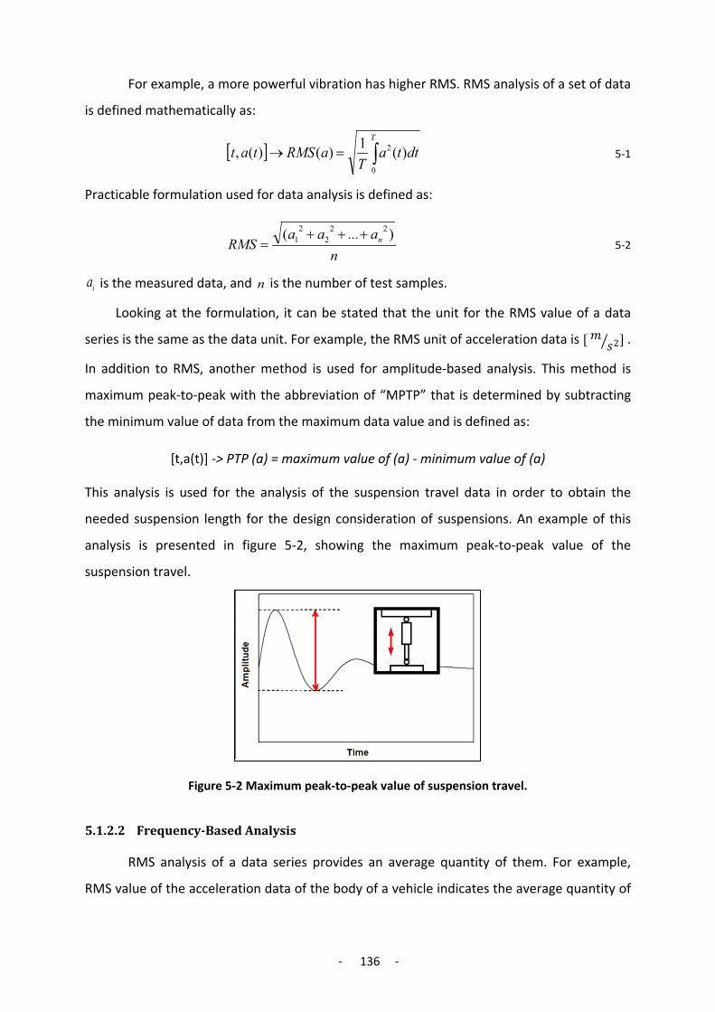
- 136 -

For example, a more powerful vibration has higher RMS. RMS analysis of a set of data

is defined mathematically as:

[ ] ∫=→T

dttaT

aRMStat0

2 )(1)()(, 5-1

Practicable formulation used for data analysis is defined as:

naaa

RMS n )...( 222

21 +++

= 5-2

ia is the measured data, and n is the number of test samples.

Looking at the formulation, it can be stated that the unit for the RMS value of a data

series is the same as the data unit. For example, the RMS unit of acceleration data is [ 𝑚𝑚 𝑁𝑁2� ] .

In addition to RMS, another method is used for amplitude-based analysis. This method is

maximum peak-to-peak with the abbreviation of “MPTP” that is determined by subtracting

the minimum value of data from the maximum data value and is defined as:

[t,a(t)] -> PTP (a) = maximum value of (a) - minimum value of (a)

This analysis is used for the analysis of the suspension travel data in order to obtain the

needed suspension length for the design consideration of suspensions. An example of this

analysis is presented in figure 5-2, showing the maximum peak-to-peak value of the

suspension travel.

Figure 5-2 Maximum peak-to-peak value of suspension travel.

5.1.2.2 Frequency-Based Analysis

RMS analysis of a data series provides an average quantity of them. For example,

RMS value of the acceleration data of the body of a vehicle indicates the average quantity of

- 137 -

ride comfort. In order to understand the quantity of ride comfort in different frequency

ranges, in addition to amplitude-based analysis, a frequency-based analysis is needed.

The common method in frequency analysis is spectrum analysis that presents a

graphical illustration from the different exciting frequencies derived from the time history

data along with the amplitude of each frequency. These graphs provide a useful tool in order

to recognize the different frequency components of a data series. In this study, a particular

spectrum method called “Power Spectral Density” or as abbreviation “PSD” is used that

instead of amplitude, presents the average of the vibration power.

PSD is defined mathematically as the average of the Fourier transform magnitude

squared, over a large time interval as follows:

= ∫−

−

∞→

2

2)(21lim)(

T

T

ftj

Tx dtetxT

EfS π 5-3

The power of x(t) in the range of (f1 -f2) is defined as:

∫=1

2

)(12

f

fx dffSP 5-4

In a PSD graph, the x-axis is the frequency with the unit of [Hz], and the y-axis is the PSD

value. The unit of the PSD values is resulting from its formulation that is the quarter of data

quantity divided by frequency unit. For example, for acceleration data, the PSD unit is (𝑚𝑚 𝑁𝑁2� )2

Hz.

In practice, estimating methods are used for sampling discrete date to perform the

PSD analysis. A standard way is to use a window function in “Discrete Fourier Transform” or

DFT. A discrete data is obtained effectively by a window w[n] function that selects a finite-

length (e.g. N samples) of x[n] from the continuous signal as follows:

[ ] [ ] [ ]nxnwnv ⋅= 5-5

The FFT of the sampled data is defined as:

[ ] [ ] nFiN

nkenxnwkV π21

0)( −−

=∑ ⋅⋅= 5-6

Where, N is the number of samples. As simplification, an estimation method can be used for

the calculation of the power spectrum as follows:

[ ]2

1

02

)()(

1)( kVnw

kP N

n∑ −

=

= 5-7

- 138 -

There are some different window functions. The simple one is the “Rectangular” window,

defined as:

[ ] 1=nw 5-8

In this study, the window function of “Hanning” is used, because it provides good

frequency resolution and leakage protection with fair amplitude accuracy. Having these

advantages, this function is became the most commonly used window functions for random

signals (Ziemer, Tranter, & Fannin, 1998). This function is defined as:

[ ]

−−=

12cos1

21

Nnnw π

5-9

5.1.3 Test Input

In order to evaluate the performance of the suspension system, response of the

system to a suspension excitation should be studied. Exciting of the suspension is performed

by the test input, which is indeed simulation of the road input. This input is a vertical

displacement wave that applies to the tires and through them excites the suspension

system.

In evaluating tests, in addition to the time domain, the frequency domain of the

system is also considered. Because of this, the test input must provide all the frequency

range of the suspension vibrations. There are different kinds of inputs waves used as the

suspension excitation for the tests. Figure 5-3 indicates the three main categories of them,

which are random, swept-frequency, and pulse inputs.

Figure 5-3 Different input signal, used for the frequency response analysis.

For this investigation, the pulse signal was used as input signal (Fig. 5-4). This input

was used for the simulation and experimental tests. Frequency of the input pulse was 10 Hz.

- 139 -

This value was selected based on the practical considerations of the test input in the

experimental tests, which were performed using a suspension test rig. The determined pulse

signal with this frequency was sufficient to cover the required bandwidth of the suspension

vibrations.

Figure 5-4 The positive and negative pulse used for the test input.

Table 5-1 Three input modes used for the tests and the relevant pulses applying to the wheels.

Pulse to Wheel

Input Mode Front Left

Front Right

Rear Left

Rear Right

Roll

Heave

Pitch

As mentioned before, the tests criteria were the parameters of the tractor body

vibrations including the vertical vibration (i.e. heave) and the rotational vibration (i.e. pitch

and roll) of the tractor body and the parameters of the vertical vibration (i.e. hip-hop) of the

wheels. In order to examine these parameters, the test input was designed so as to provide a

direct excitation on each one of these parameters. For this purpose, the input pulses were

applied to the four tires of the tractor in three special orders called: roll, heave, and pitch

modes. These inputs create direct excitations for the vertical and rotational vibrations. Table

5-1 shows these three input modes and determines the direction (i.e. positive or negative) of

each pulse, which is applied to a tire in order to perform the three input modes.

- 140 -

5.1.4 Test Plan

In the previous sections, the test input, output, and data reduction were determined.

At this point, the plan of the whole tests including the simulation and experimental tests can

be formulated. In this plan, the inputs and outputs of each test should be determined. In

addition, the measuring parameters and data reduction method of each test should be

resolved.

Table 5-2 presents a plan for the tests including inputs, outputs, measuring

parameters, and data reduction method for each test. This plan consists of two similar test

groups; the first with passive suspension mode and the second with semi-active suspension

mode, that are considered concerning to the main objective of this study as evaluation of the

new suspension by comparing it with conventional passive suspension.

On the other hand, model validation is an objective of this investigation. In order to

perform the model validation, the results of the simulation tests should be compared with

the experimental tests. Therefore, it is needed that the test design for the simulation and

experimental tests would be similar. This includes the test input, test output, and the test

plan. However, the repetitions of the two test groups are different. This issue will be

discussed in the following sections. As shown in table 5-2, there is a similar plan for both

groups of the tests. At the final columns of the table, results of the simulation and

experimental tests are shown separately.

There are three types of outputs for the tests. The first one includes the heave, pitch,

and roll accelerations of the tractor body, which are used for evaluating the ride comfort.

The second one is the dynamic tire vertical forces, which are used for evaluating the

handling ability of the tractor, and the third one is the suspension travel, which is considered

for suspension design consideration.

The corresponding test inputs to the test outputs are also determined in table 5-2.

The roll input mode is used for the body roll acceleration and the heave input mode is used

for body heave acceleration. The input mode of pitch is considered for the dynamic tire force

and suspension travel, in addition to body pitch acceleration.

In the table of the test plan, the data reduction method for each output of the tests is

determined. For the heave, pitch, and roll accelerations of the tractor body both RMS and

PSD as amplitude and frequency based analysis are considered. Similar analysis is considered

for the dynamic tire force, and for the suspension travel, MPTP amplitude-based analysis is

- 141 -

determined. In the last column of the table, the final reduced data of the tests are listed.

Repetition of each test is not considered in this table. This subject will be explained in the

following section during the description of the simulation and experimental tests.

Table 5-2 Detailed tests plan.

Test Suspension

Mode Input

Measuring Parameter

Output Data

Analysis (Exp.)

Data Nr. (Sim.)

Data Nr.

T01 Passive Roll Body corners acc. Roll acc. RMS &

PSD

e1 s1

e2 s2

T02 Passive Pitch 1-Body corners acc. 2-Wheels acc. 3-Sus. travel

Pitch acc. RMS &

PSD

e3 s3

e4 s4

Tire force RMS &

PSD

e5 s5

e6 s6

Sus. travel MPTP e7 s7

T03 Passive Heave Body corners acc. Heave acc. RMS &

PSD

e8 s8

e9 s9

T04 Semi-active

Roll Body corners acc. Roll acc. RMS &

PSD

e10 s10

e11 s11

T05 Semi-active

Pitch 1-Body corners acc. 2-Wheels acc. 3-Sus. travel

Pitch acc. RMS &

PSD

e12 s12

e13 s13

Tire force RMS &

PSD

e14 s14

e15 s15

Sus. travel MPTP e16 s16

T06 Semi-active

Heave Body corners acc. Heave acc. RMS &

PSD

e17 s17

e18 s18

In this section, the test plan was presented. The input, output, and data reduction

method of the tests were also explained. At this point, the tests can be performed. In the

following sections, performance of the simulation and experimental tests will be described.

5.2 Simulation Tests

Figure 5-5 shows the procedure of the simulation tests. In the previous sections, the

test plan, test input, test output, and data reduction were explained before. In this section,

performing of the simulation tests is presented. First, the preparation of the full tractor

Simulink model for these tests is explained. Then, the execution of the tests is described.

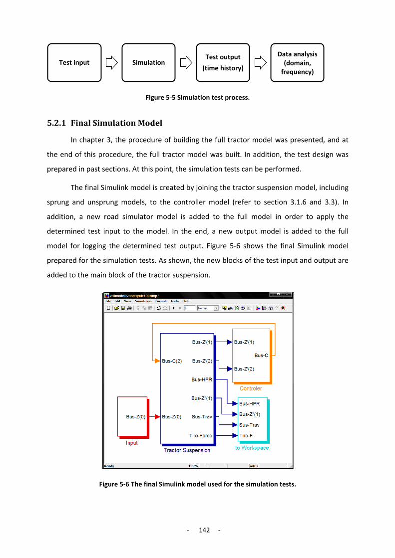
- 142 -

Figure 5-5 Simulation test process.

5.2.1 Final Simulation Model

In chapter 3, the procedure of building the full tractor model was presented, and at

the end of this procedure, the full tractor model was built. In addition, the test design was

prepared in past sections. At this point, the simulation tests can be performed.

The final Simulink model is created by joining the tractor suspension model, including

sprung and unsprung models, to the controller model (refer to section 3.1.6 and 3.3). In

addition, a new road simulator model is added to the full model in order to apply the

determined test input to the model. In the end, a new output model is added to the full

model for logging the determined test output. Figure 5-6 shows the final Simulink model

prepared for the simulation tests. As shown, the new blocks of the test input and output are

added to the main block of the tractor suspension.

Figure 5-6 The final Simulink model used for the simulation tests.

Test input Simulation Test output

(time history)

Data analysis(domain,

frequency)

- 143 -

Figure 5-7 shows the Simulink model of the test-input simulator. This model is

created based on the input test defined in section 5.1.3. Using the Simulink block of “signal

builder” and based on the figure 5.4, the simulator of the input signal is built. In addition, the

produced pulse is divided into four tractor tires according to the table 5-1 in order to

simulate three input modes.

Input Mode

Suspension Unit

fl fr rl rr

Roll +1 -1 +1 -1

Heave +1 +1 +1 +1

Pitch -1 -1 +1 +1

Figure 5-7 Simulink model of the test input simulator with the relevant input-modes coefficients.

For logging the outputs of the simulation tests, the determined parameters are sent

directly to the “workspace” and saved as time history data. However, the dynamic tire forces

are not available as the direct parameters in the model, and they are calculated through

other parameters. After the calculation of these data, they are sent to the workspace and

saved as time history data. Figure 5-8 indicates the Simulink model of the calculator of the

dynamic tire force. The inputs of this model are the displacement of the road simulator and

the displacement of the wheel.

Figure 5-8 Simulink calculator of the dynamic tire force.

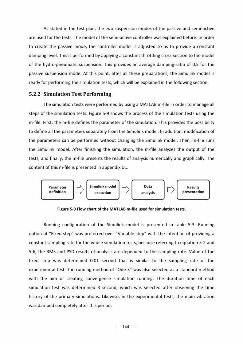
- 144 -

As stated in the test plan, the two suspension modes of the passive and semi-active

are used for the tests. The model of the semi-active controller was explained before. In order

to create the passive mode, the controller model is adjusted so as to provide a constant

damping level. This is performed by applying a constant throttling cross-section to the model

of the hydro-pneumatic suspension. This provides an average damping-ratio of 0.5 for the

passive suspension mode. At this point, after all these preparations, the Simulink model is

ready for performing the simulation tests, which will be explained in the following section.

5.2.2 Simulation Test Performing

The simulation tests were performed by using a MATLAB m-file in order to manage all

steps of the simulation tests. Figure 5-9 shows the process of the simulation tests using the

m-file. First, the m-file defines the parameter of the simulation. This provides the possibility

to define all the parameters separately from the Simulink model. In addition, modification of

the parameters can be performed without changing the Simulink model. Then, m-file runs

the Simulink model. After finishing the simulation, the m-file analyzes the output of the

tests, and finally, the m-file presents the results of analysis numerically and graphically. The

content of this m-file is presented in appendix D1.

Figure 5-9 Flow chart of the MATLAB m-file used for simulation tests.

Running configuration of the Simulink model is presented in table 5-3. Running

option of “Fixed-step” was preferred over “Variable-step” with the intention of providing a

constant sampling rate for the whole simulation tests, because referring to equation 5-2 and

5-6, the RMS and PSD results of analysis are depended to the sampling rate. Value of the

fixed step was determined 0.01 second that is similar to the sampling rate of the

experimental test. The running method of “Ode 3” was also selected as a standard method

with the aim of creating convergence simulation running. The duration time of each

simulation test was determined 3 second, which was selected after observing the time

history of the primary simulations. Likewise, in the experimental tests, the main vibration

was damped completely after this period.

Parameter definition

Simulink model

execution

Data

analysisResults

presentation

- 145 -

Table 5-3 Simulink software configuration used for the simulation tests.

Solver Parameters

Fixed-step Type: Ode 3 (Bagacki-Shanpine) Method: 0.01 sec. Fixed-step size: 3 sec. Simulation time:

The simulation tests, based on the test plan, were performed in two categories:

passive suspension mode and semi-active suspension mode. Adjusting a test input, the test

was performed once in the semi-active suspension mode. Then, the second corresponding

test was performed with the same input in the passive suspension mode. Since no random

function was used in the model and simulation, the repetition of each simulation test was

not required. However, in order to ensure the repeatability and correctness of the tests,

each simulation test was repeated once.

5.3 Experimental Tests

The building a prototype for the system was explained in chapter 4. This model was

used for the experimental tests. The test plan of the experimental tests was similar to the

simulation tests. Before performing the experimental tests, the necessary preparation was

organized. Figure 5-10 illustrates the configuration of the experimental tests. In order to

create the test input and test output in the experimental tests, two new components of

excitation unit and data logging unit were used. The excitation unit provided the test input in

order to excite the suspension system, and data logger was used in order to measure the

output parameter and to save them. These data were analyzed in the next step.

Figure 5-10 Experimental test configuration.

Sensors

Controller Actuator Test-tractor

Excitation

Data logging

Test Input

Test Output

- 146 -

In this section, first, the suspension test rig used for applying the test input to the

test-tractor is explained. Then, the data logging system used for measuring and saving the

test output is described. After that, the operation check of the control system is explained,

and finally, performing of the experimental tests is presented.

5.3.1 Full Suspension Test Rig

For performing the experimental tests and applying the test input to the test-tractor,

there were two options: field testing and laboratory testing. As this study was the first

attempt in evaluating the new suspension system after the creation of it, the first option was

considered as the best choice. This option was the performing of laboratory tests by using a

suspension test rig. For this purpose, the suspension test rig at the TU Berlin - Department

Machinery System Design was used as a road input simulator. By using these facilities, it was

possible to perform the test excitation and data logging accurately and without different

error sources, which exist in typical field testing.

This suspension test rig consists of four hydraulic shakers. As shown in figure 5-11,

the tractor stayed on the test rig so that each shaker was placed under one wheel, and so

the wheels could be excited individually. The framework of the test rig is mounted on a

foundation via an air suspension system in order to isolate ground from the test rig

vibrations.

Figure 5-11 Test-tractor standing on the full suspension test rig.

Tractor-Test

Test Rig Hydraulic Cylinder

Test Rig units

Test Rig units

Test Rig Framework

- 147 -

The control center of the suspension test rig is shown in figure 5-12. This system is

able to control each hydraulic shaker independently with individual waveform and

amplitude. The input of each shaker can be adjusted separately. Each shaker is indeed a

double-acting hydraulic cylinder, controlled by a servo-valve. This servo-valve receives

command signal from the control center. Technical data of the suspension test rig is

presented in appendix B.

For applying the determined input signal to the suspension test rig, a function

generator was used to create proper signals correspondent to the input signal illustrated in

figure (5-4). Amplitude and waveform of the control commands, which were sent to the

shakers, were monitored by an oscilloscope (Fig. 5-12). Amplitude of the input test created

by shaker was adjusted to the value of plus or minus five cm. Then, this input signal was

applied to each shaker with a special order, which was indicated before in table 5-1.

Figure 5-12 Equipment of the control system of the full suspension test rig.

The suspension test rig was used for applying the test inputs to the test tractor. For

output of tests, a data acquisition system was used in order to gather the data from the

output parameters of tests. This subject will be described in the following section.

5.3.2 Data Acquisition System

Data acquisition system conducted two functions: measurement and data logging.

The output parameters of the tests were measured by using suitable sensors, and the signals

of these sensors were saved by data logger as time history data. These saved data were later

analyzed in order to derive the test results.

Function Generator

Test Rig Control Devices

Oscilloscope

- 148 -

The data acquisition system used for this research was a PC-based system including a

laptop computer connecting to a sensory set-up via an ADC interface card (Fig. 5-13 and 5-

14). The sensory set-up consisted of the sensors, signal conditioner, and a low-pass filter.

The sensors measured the determined parameters. The signals of the sensors were

converted firstly to the proper type of signals, because signals of the sensors should be

compatible with the inputs of the interface card. For this purpose, a signal conditioner was

used.

Conditioning of the signals was composed of sensor excitation, sensor isolation, and

signal amplification. Before signals enter to the card, they were passed through a 20Hz low-

pass filter. This filter separated the signals of the sensors from the noise and from the high

frequency signals, which are not related to the suspension operation. Then, the sensory

signals were converted to digital signals by using ADC card and after that, were saved by

computer as time history data. The saved data was later transferred to another PC in order

to perform the needed analysis on them.

Figure 5-13 Components of the data acquisition system.

Figure 5-14 Schematic configuration of the data acquisition system (Thiebes P. , 2006).

The ADC interface Card used for data logger system was PCI-BASE300 from BMC

Company working with the nextView NT Software. This cart was equipped with 16 analog

inputs with the resolution of 16 bits. The sampling rate of the data logging system was 100

Hz. Technical data of this card is presented in appendix C5.

Sensors Signal conditioner

Low-Pass filter (20Hz)

Interface card Laptop

- 149 -

As mentioned, the output parameters of the tests were measured by data acquisition

system. These outputs were chosen based on the performance criteria. The output

parameters were accelerations of the center of gravity of the tractor body, dynamic tire

force, and suspension travel (section 5.1.1). However, except the suspension travel, it was

not possible to measure these parameters directly. Therefore in order to acquire these

parameters, initially some related parameters were measured. Then based on these values

and using relevant equation, the main parameters were derived. This procedure is illustrated

in figure 5-15.

Figure 5-15 Analysis procedure of the experimental data.

The acceleration of the center of gravity of the tractor body including heave, pitch,

and roll acceleration were calculated based on the vertical acceleration data, measured on

the body corners. The calculation was accomplished by using the following equations, which

are taken from section 3.1.5 based on the figure 3-6.

⎩⎪⎪⎨

⎪⎪⎧

ϕθ ′′+′′−′′=′′ ..z2fl lfcg tlz

ϕθ ′′−′′−′′=′′ ..z2fr rfcg tlz

ϕθ ′′+′′+′′=′′ ..z2rl lrcg tlz

ϕθ ′′−′′+′′=′′ ..z2rr rrcg tlz

� 5-10

In order to solve this system of linear equations, they were represented in the matrix form

as:

BXA =⋅

The unknown matrix X consisted of the accelerations of the center of gravity, and constant

matrix B consisted of the vertical accelerations of the body corners. Matrix A also consisted

of the dimensional parameters of the tractor. So, the system of linear equations was

presented as:

Saved data [time,a]

Data

calculationTest output

Accelerations data

Using MATLAB m-file

-Heave, pitch & roll of CG

-Dynamic tire force

- 150 -

′′′′′′

=

′′′′′′

−−

−

2rl

2fr

2fl

zzz

.111

ϕθ

cg

lr

rf

lf z

tltl

tl 5-11

By multiplication of the two sides of the equation by the inverse of the matrix of the

dimensional parameters (i.e. A), the system of linear equations was solved, and the matrix of

the accelerations of the center of gravity (i.e. X) was obtained as:

BAX ⋅= −1 5-12

In addition to the acceleration on the center of gravity, the dynamic tire force should be

calculated from the measured parameters. For this purpose, the formulation of the quarter

car model (i.e. the equations of the sprung and unsprung masses) from section 3.1.2 was

used as follow:

02222 =++″+ ck FFzm

0221111 =−−++″+ ckck FFFFzm

After some manipulations, a new equation was resulted as:

01122 11=″+++″+= zmFFzmF ckt 5-13

On the other hand, the dynamic tire force was equal as:

11 ckt FFF −−= 5-14

Therefore, the dynamic tire force was obtained based on the vertical accelerations of the

wheel and body corner as:

″+″+= 1122 zmzmFt 5-15

By writing a m-file in MATLAB the mentioned calculations of the body acceleration

and dynamic tire force were performed overall experimental data. This program read the

measured parameters, which were saved by data logger before. Then, by using the

formulation explained in this section, it gives the time history of the calculated parameters.

This m-file is presented in appendix D2.

As mentioned, the output parameters were obtained indirectly some other

measurable parameters. The list of these measured parameters is presented in table 5-4.

Four accelerometers, placed on the corners of the tractor body, were used to measure the

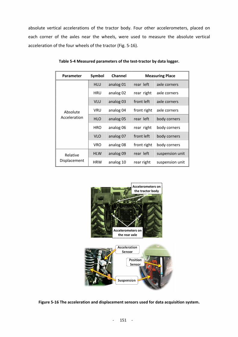
- 151 -

absolute vertical accelerations of the tractor body. Four other accelerometers, placed on

each corner of the axles near the wheels, were used to measure the absolute vertical

acceleration of the four wheels of the tractor (Fig. 5-16).

Table 5-4 Measured parameters of the test-tractor by data logger.

Measuring Place Channel Symbol Parameter

axle corners rear left analog 01 HLU

Absolute Acceleration

axle corners rear right analog 02 HRU

axle corners front left analog 03 VLU

axle corners front right analog 04 VRU

body corners rear left analog 05 HLO

body corners rear right analog 06 HRO

body corners front left analog 07 VLO

body corners front right analog 08 VRO

suspension unit rear left analog 09 HLW Relative Displacement suspension unit rear right analog 10 HRW

Figure 5-16 The acceleration and displacement sensors used for data acquisition system.

Accelerometers on the tractor body

Accelerometers on the rear axle

- 152 -

For measuring suspension travel, two displacement sensors were employed. For

measuring the displacement, linear resistor-type of the position transducers were used (Fig.

5-16). Accelerometers were piezo-resistive type with the measuring range of ±20𝐾𝐾 for the

wheel acceleration and with the measuring range of ±10𝐾𝐾 for the body acceleration. The

detailed specifications of the acceleration sensor are given in appendix C1.

5.3.3 System Operation Check

Before using developed prototype for performing the experimental tests, relevant

adjustment were done, and operation of the different components were proved separately.

For this purpose, at first, the hydro-pneumatic suspension was re-examined. Different

components of this system were considered separately. The proved parameters of these

components were the initial gas pressure of the accumulators, primary suspension height,

valves connections, and passive and semi-active modes of the throttle valves.

Suspension characteristic of the tires has a significant influence on the suspension

performance of a tractor. This characteristic is directly dependent on the inflation pressures

of tires. For more details about the suspension characteristic of the tires, please refer to

section 2.5.1. Therefore, after the hydro-pneumatic suspension, tractor tires were proved to

be with the correct determined inflation pressures. In addition, the data acquisition system

including sensors, signal conditioner, and pc-based data logger were calibrated and

confirmed.

At this point that the test-tractor was placed on the suspension test rig and was ready

for the tests (Fig. 5-11), a check on the electronic components of the control system was

done before performing the tests. For this purpose, the data logging system was arranged in

order to measure the output of each component. Figure 5-17 shows the configuration of this

primary test.

Figure 5-17 Configuration of the primary test of the control system.

Data Logger

PC

ADC Interface Relay Sensors Filter Test Rig

- 153 -

The test was started with applying a test input to the suspension test rig. The data

logger using a position sensor measured the real output of the test rig. Time-history data of

the output signal of all components were saved by data logger. These components were

sensors, low pass filter, A/D converter, interface card, and electronic relay. Using these data,

after the test, operation of each component was examined.

For example, figure 5-18 shows the saved time history data measured by the absolute

and relative velocity sensors that were used as the inputs of the tests along with the

electronic relay signals as the output of control. As shown, the noise effect of the sensors

signals caused some errors in the signals of the relays, which is applied to the valves in the

real system. Recognizing this problem, in order to overcome against it a low-pass filter was

used after the sensors in order to remove the noise part of the sensory signals.

Figure 5-18 A result of the primary controller test, indicating mistakes in the relay signals due to the noise effect.

Another characteristic of the control system that should be revealed was the system

bandwidth. The every part of control system worked in a close loop (Fig. 5-19). In order to

determine system bandwidth, the spending time of each component was considered. In

developing of the system, it was a challenge to fulfill the required control bandwidth.

Therefore, during the designing of the system, time response of each component of

the system was carefully determined. The system consisted of two categories of

components: the electronic components and the electro-mechanic components. The

electronic components were PC, I/O card, electronic relay, A/D converter, and low-pass

filter. The electro-mechanic components were the velocity transducers and solenoid valves.

- 154 -

Figure 5-19 Semi-active close control loop.

By using fast electronic components, especially I/O card, A/D converter, and

electronic relay, a high bandwidth value of about 300 Hz was achieved. This value measured

by creating close loop running of the system without electro-mechanic components. Among

electro-mechanic components, whereas the velocity transducers had no significant delay in

their operation, the valves created main delay in the system. Therefore, the delay time of

the valves was the single factor that established the bandwidth of the control system and

was concerned in the selection of these valves.

The valve delay was studied during the valve modeling presented in section 3.2.2.4.

The delays of the solenoid valves of this project were between 20 ms and 35 ms, referring to

their data sheet. Therefore, the whole delay of the control loop was determined maximum

40 ms that meant that the bandwidth of the system was at least 25 Hz.

This bandwidth was acceptable for the control system in this research, because the

goal of this research was the effective damping of the vibration of the tractor body. The

natural frequencies of the tractor body, which were obtained from the primary tests, were

maximum 2 Hz. On the other hand, the natural frequency of the wheels (i.e. unsprung mass)

was 5 Hz. As a result, these frequencies were covered by 25 Hz bandwidth of the control

system.

As described, by primary operation check of the system components, the correction

of the system operation was confirmed, and necessary adjustment was performed. As the

next step, the experimental tests were performed, which will be explained in the following

section.

PC

Out. Card

Relay

Electro-valve

Sensors

Filter

ADC

Inp. Card

- 155 -

5.3.4 Experimental Test Performing

In order to perform the experimental evaluation of the new suspension system, the

experimental tests were considered. For this purpose, as described in the previous chapter, a

prototype of the system was built. A test plan was determined, and the related test setup

was arranged. At the end, a check on system was performed. At this point, after all these

preparations, the experimental tests could be begun.

For performing the experimental tests, the control equipments were placed all in the

driver cabin (Fig. 5-20). These equipments consisted of interface card, low-pass filter, signal

conditioner, and electronic relay system. After that, test-tractor was placed on the

suspension test rig (Fig. 5-21).

Figure 5-20 Electronic equipment installed in the tractor cabin used for the experimental test.

Figure 5-21 Rear view of the test-tractor standing on the full suspension test rig used for the experimental tests.

Low-Pass Filters

Interface Card

Relay System

Signal conditioner

Controller Devices Hydro-

pneumatic system

Suspension Test units

- 156 -

Interface card was connected to the controller PC via a long USB cable, which was

placed in the controller room of the test rig (Fig. 5-22). Applying the proper input to the test

rig, monitoring of the semi-active controller, and data logging system were performed from

this room.

Figure 5-22 A view of the PC-based controller located in the test rig control cabin.

Performing of the experimental tests was based on the test plan presented in table 5-

2. First, hydro-pneumatic rear suspension was tuned in the passive mode. For this purpose,

the controller was turned off, and the throttle valve was tuned to the passive mode in order

to provide the standard damping level. Then, the input mode was selected, and the

controller of the suspension test rig was adjusted according to the arrangement in table 5-1.

After that, the data logger was turned on a new data file with specific name, and the

test was performed by applying the “Roll” input signal to the test rig. The second repetition

of the tests was performed after a period time in order to ensure that the vibrations of the

tractor are damped completely. Then, the third and forth attempts were performed

similarly, and finally, with closing the data file this test was finished.

The second and third test groups were performed with applying the “Pitch” and

“Heave” input signals to the test rig. Each test category was performed similar to the “Roll”

test. However, the data was saved with a new data file by data logger. Therefore, in the

passive suspension mode, three data files including data of the 12 tests were achieved as the

result of the tests.

After this test category of the passive suspension mode, the test category of the

semi-active suspension mode was performed. For this propose, firstly, the hydro-pneumatic

rear suspension was tuned on the semi-active mode. In this mode, the controller was tuned

PC-Based Controller

Trtactor on Test stand

Controller Software

Cable to Controller

- 157 -

on, and the throttle valve was tuned in the semi-active mode (i.e. low damping mode). Other

steps of the test were similar to the test category of the passive mode. At the end, three

data file including the data of the 12 tests, were achieved as the results of the tests.

As mentioned, each individual test was repeated four times in order to increase the

reliability of the tests and decrease the influence of unexpected errors. For analyzing of the

test data, the RMS, MPTP, and the PSD results of each repeat of the tests were calculated

separately. Then, the average of the four repeats was considered as main result. These

calculations were performed by using an m-file program in MATLAB software.

This program received the data files related to the four repeats of the experimental

tests, and based on these data, calculated the output of the tests. The formulation of this

calculation was presented in section 5.3.2. In addition, this program calculated the average

values of the RMS, MPTP, and PSD analysis of the test outputs. The content of this m-file

program is presented partly in appendix D1.

- 158 -

Chapter 6

6 Result

After describing the execution step of the simulation and experimental tests, in this

chapter, the achieved results from these tests are presented. These results are presented in

four groups, which are respectively: model validation results, ride comfort results, handling

results, and suspension stroke results. At first, the results of the model validation are

presented by comparison of the simulation tests results with the experimental tests results.

Then, performance of the new suspension system concerning the ride comfort of the

tractor is evaluated by comparison of the passive suspension results with the semi-active

suspension results for both the simulation and experimental tests. Likewise, the

performance of the new suspension system concerning the handling capability of the tractor

is evaluated. After that, the influence of the new suspension system on the suspension travel

is examined by comparison of the passive suspension results with the semi-active suspension

results for the simulation and experimental tests. Finally, all these results are summarized.

6.1 Model Validation

Along with the experimental and simulation studies, the validation of the simulation

model was considered also as an objective of this research work. This was performed by

comparison of the simulation result with the corresponding experimental results. After the

validation of the model, the results of the simulation test could be used for the evaluation of

the new suspension system by the simulation tests as well as the experimental tests. In

addition, this model can be used for future developing investigations in the area of the

suspension systems for agricultural tractors.

Figure 6-1 shows the procedure of the model validation. Each simulation result was

compared with the corresponding experimental result. The simulation model was examined

in order to recognize the weak points of the model and increase the correlations between

simulation and experimental results.

- 159 -

Figure 6-1 Model validation procedure.

Basically, low precise result appears in a simulation model because of the failure in

the logic of the modeling or in the imprecise parameters of the simulation. In the validation

process in this investigation, modification of the simulation model was performed by

considering these two inaccuracy sources. For instance, in the case of the failure in modeling

logic, after observing a low correlation in time and frequency domain results, it was realized

that the hydraulic cylinder model should be modified by considering the friction effect in the

model.

Therefore, as described in section 3.2.3, the model of the friction effect in the

cylinders was built and added to the main cylinder model. In another case, observing low

correlation in the natural frequency results led to consider a multi-body lumped-mass model

for the tractor body model. In addition, parameters that are more accurate were derived for

the tractor masses. These multi-body mass model and the relevant parameters are

presented in appendix E.

The validation was performed based on the comparative results of the simulation and

experimental tests in two categories of the time domain and frequency domain results.

These results will be presented in the following sections. It should be noted that the

simulation results of this part are the simulation results that were achieved after the model

validation.

6.1.1 Amplitude-Based Validation

The amplitude-based validation of the model was performed using RMS values in the

following formula. In this formula, which gives the percentage inaccuracy of the simulation

results, experimental results are considered as the reference.

Simulink

modelSimulation

test

Virtual prototype

Experimental test

Results

comaprisonCorrelation

(?) End

Weak

Strong

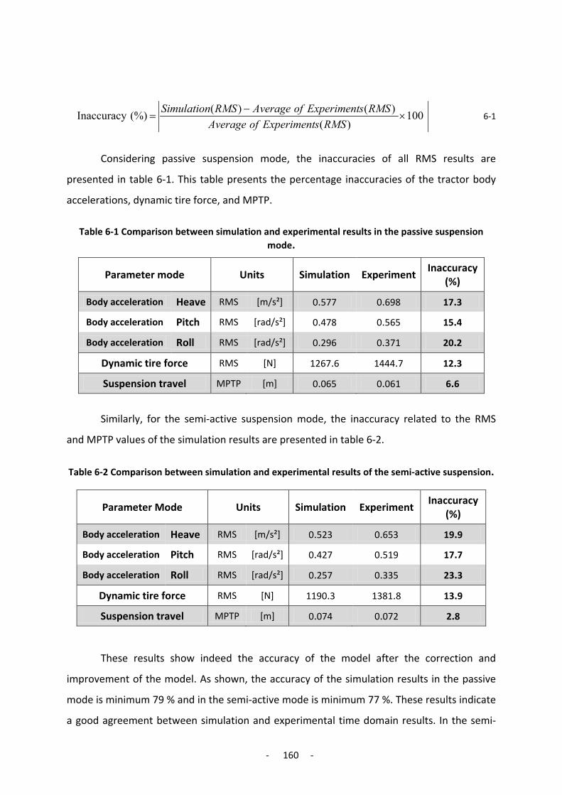
- 160 -

100)(

)()((%) Inaccuracy ×−

=RMSsExperimentofAverage

RMSsExperimentofAverageRMSSimulation 6-1

Considering passive suspension mode, the inaccuracies of all RMS results are

presented in table 6-1. This table presents the percentage inaccuracies of the tractor body

accelerations, dynamic tire force, and MPTP.

Table 6-1 Comparison between simulation and experimental results in the passive suspension mode.

Parameter mode Units Simulation Experiment Inaccuracy

(%)

Body acceleration Heave RMS [m/s²] 0.577 0.698 17.3

Body acceleration Pitch RMS [rad/s²] 0.478 0.565 15.4

Body acceleration Roll RMS [rad/s²] 0.296 0.371 20.2

Dynamic tire force RMS [N] 1267.6 1444.7 12.3

Suspension travel MPTP [m] 0.065 0.061 6.6

Similarly, for the semi-active suspension mode, the inaccuracy related to the RMS

and MPTP values of the simulation results are presented in table 6-2.

Table 6-2 Comparison between simulation and experimental results of the semi-active suspension.

Parameter Mode Units Simulation Experiment Inaccuracy

(%)

Body acceleration Heave RMS [m/s²] 0.523 0.653 19.9

Body acceleration Pitch RMS [rad/s²] 0.427 0.519 17.7

Body acceleration Roll RMS [rad/s²] 0.257 0.335 23.3

Dynamic tire force RMS [N] 1190.3 1381.8 13.9

Suspension travel MPTP [m] 0.074 0.072 2.8

These results show indeed the accuracy of the model after the correction and

improvement of the model. As shown, the accuracy of the simulation results in the passive

mode is minimum 79 % and in the semi-active mode is minimum 77 %. These results indicate

a good agreement between simulation and experimental time domain results. In the semi-

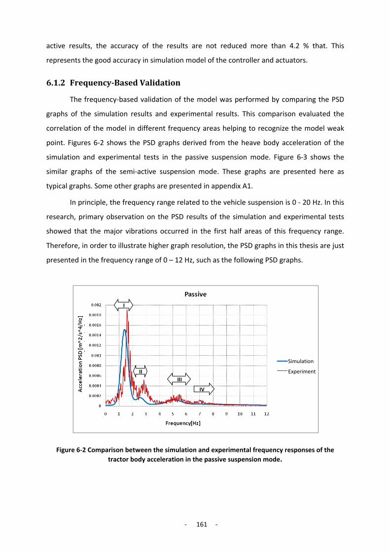
- 161 -

active results, the accuracy of the results are not reduced more than 4.2 % that. This

represents the good accuracy in simulation model of the controller and actuators.

6.1.2 Frequency-Based Validation

The frequency-based validation of the model was performed by comparing the PSD

graphs of the simulation results and experimental results. This comparison evaluated the

correlation of the model in different frequency areas helping to recognize the model weak

point. Figures 6-2 shows the PSD graphs derived from the heave body acceleration of the

simulation and experimental tests in the passive suspension mode. Figure 6-3 shows the

similar graphs of the semi-active suspension mode. These graphs are presented here as

typical graphs. Some other graphs are presented in appendix A1.

In principle, the frequency range related to the vehicle suspension is 0 - 20 Hz. In this

research, primary observation on the PSD results of the simulation and experimental tests

showed that the major vibrations occurred in the first half areas of this frequency range.

Therefore, in order to illustrate higher graph resolution, the PSD graphs in this thesis are just

presented in the frequency range of 0 – 12 Hz, such as the following PSD graphs.

Figure 6-2 Comparison between the simulation and experimental frequency responses of the tractor body acceleration in the passive suspension mode.

Simulation

Experiment

I

III II

IV

- 162 -

Figure 6-3 Comparison between the simulation and experimental frequency responses of the tractor body acceleration in the semi-active suspension mode.

These results are indeed the comparison of the experimental result with the results

of the validated simulation model. As the first different, simulation curve is smooth and

experimental curve is jagged. This is so, because the tractor body model was simplified to

the lumped solid-mass model, whereas in reality, tractor body consists of mass-components

(i.e. multi-body) with elastic connection. However, as shown the main curves demonstrate a

good agreement. In order to analyze these graphs, the frequency area is divided into four

areas.

The first area is the frequency range from 0.5 to 2 Hz, containing tractor body (sprung

mass) natural frequencies. As shown, there is a good agreement between two curves, and

just the frequency of the peak amplitude is a little different. The quantity of this difference

will present in the end of this section.

The second area is the frequency range from 2 to 4 Hz. This area is placed between

the two areas of the natural frequencies of the sprung mass and unsprung mass. As shown,

in this area on the experimental curve, there is an unknown peak amplitude. Before the

validation of the model, in the simulation curve, this peak did not exist. An estimated

computation showed that the frequency of this peak (~3 Hz) is comparable with natural

frequency of the tractor body when there would be solid connection between the body and

wheel. Primary experimental observation indicated that this peak occurred because of the

slip-stick effect in the suspension elements. In order to provide a better agreement between

IV

Simulation

Experiment

I

III II

- 163 -

simulation and experiment curves in this area, the friction model of the cylinder was added

to the main model (described in section 3.2.3). After that, a similar peak appeared in the

simulation curve in this area (Fig. 6-2, 6-3).

The third area is the frequency range between 4 and 6.5 Hz. This area contains

particularly the natural frequency of the wheels (i.e. unsprung mass). As shown, there is a

good agreement between the two curves, and just the frequency of the peak amplitude is a

small amount different. The quantity of this difference will be presented in the end of this

section.

Frequency range further than 6.5 Hz is the fourth area, which contains the natural

frequencies related to the minor mass-components of the tractor. Except a minor peak

amplitude in the experimental curve, there is no considerable peak in this area. This peak is

indeed the natural frequency of the cabin, which is attached to the tractor body through a

rubber connection operating as a semi-suspension and has its individual natural frequency.

Since this system had not significant effect on the results of the experimental tests, it was

not considered in the simulation model. Consequently, the effect related to this system does

not exist in the simulation curve.

As shown from the PSD graphs, the experimental curves show generally a little higher

amplitude than simulation curve. As shown before, this phenomenon was more obvious in

the amplitude-based results of the validation. As mentioned, in the validation procedure,

some modifications in modeling logic and the model parameters were done, such as adding

the friction model, adding the muliti-body mass model, and using the more accurate mass

parameters. Therefore, a better agreement between general amplitude level of the

simulation and experimental results was achieved. This improvement was particularly

notable in the second area of the PSD graph that was affected by the static friction factor in

the suspension system.

The frequency-based method for validation of the model is the comparison of the

different natural frequencies of the tractor, which are derived from the simulation and

experimental tests. As mentioned before, corresponding to each degree of freedom of the

model, a natural frequency can be derived from the simulation results. Therefore, seven

natural frequencies related to the seven degrees of freedom of the model are considered.

Heave, pitch, and roll motion of the tractor body are three of them, and the rest four

frequencies are the natural frequencies of the four tractor wheels. Since the tires and mass

- 164 -

parameters of the four wheels are similar, the four natural frequencies of the wheels are the

same, and in validation study, the frequency of the just one of them is considered.

Table 6-3 presents the five natural frequencies, derived from the simulation and

experimental results. Percentage validation of the simulation results are also presented in

this table. As seen, these percentage results are at least 67 %, showing an acceptable

agreement between simulation and experimental natural frequencies.

Table 6-3 Comparison between simulation and experimental natural frequencies of the tractor.

Vibration Mode

Natural Frequency Min. Validation

[%] Experiment

[Hz] Simulation

[Hz]

Body Heave ≈1.6 1.4 78

Body Pitch ≈1.7 1.6 84

Body Roll ≈1.0 0.8 67

Wheel Hop ≈5.4 5.1 88

In the whole, after attaining acceptable correlations between the time domain and

frequency domain results of the simulation and experimental tests, the model validation was

completed, so that it can be used in order to simulate the dynamic behavior of an

agricultural tractor by focusing on the suspension system. After this validation, the results of

the simulation tests were used for the evaluation of the new suspension system besides the

experimental tests, as the secondary reference. This led to a more accurate system

evaluation. In the following sections, these results will be presented.

6.2 Ride Comfort Evaluation

The first criterion for evaluating the semi-active suspension is the ride comfort. For

this purpose, as stated before, accelerations of the tractor body were considered. The

performance of the new suspension system was evaluated by comparing the time domain

and frequency domain results of the passive suspension mode with the semi-active

suspension mode. In this section, the results of the simulation tests and then, the results of

the experimental tests are given. In each part, the time domain results and the frequency

domain results of the tests are presented.

- 165 -

6.2.1 Simulation Result

Evaluation of the suspension system, based on the time domain results, was

performed by comparing the RMS value of accelerations. In order to quantify this

comparison, the following equation was used for calculating the percentage improvement of

ride comfort. The accelerations magnitudes on the center of gravity of the tractor body are

presented in table 6-4. This data were obtained from the simulation tests. These include the

heave, pitch, and roll accelerations of the passive and semi-active suspension.

In addition, improvement of ride comfort, based on the RMS values of accelerations

is denoted in percentage by means of equation 6-2, which is presented in the last column of

this table.

100)()((%) ×−−

=RMSpassive

RMSpassiveRMSactivesemitimprovemen

6-2

Table 6-4 Simulation RMS results of the tractor body accelerations with passive and semi-active suspension.

Body Acceleration

Units Passive (RMS)

Semi-active (RMS)

Improvement [%]

Heave [m/s²] 0.577 0.523 9.4

Pitch [rad/s²] 0.478 0.427 10.7

Roll [rad/s²] 0.296 0.257 13.3

As shown, the improvements are between 9.4 % and 13.3 %. Considering that the

semi-active control was applied just to the rear suspension of the tractor, these results

indicate a good performance for the new suspension in reducing the accelerations level on

the tractor body, and means that a considerable improvement in the ride comfort of the

tractor was achieved.

The RMS analysis gave quantitative information about the average performance of

the system. After that, in order to examine the detailed operation of the semi-active system

in different frequency ranges, the frequency analysis of data was considered, which was

performed by study of the related PSD graphs. Figure 6-4 shows on of these graphs derived

from the vertical acceleration on the tractor body in the passive and semi-active suspension

modes.

- 166 -

As seen, the frequency area of this graph can be divided into four ranges. The first

area is the frequency range between 0.5 and 2 Hz, which contains the natural frequencies of

the tractor body (i.e. sprung mass). As shown, the best performance of the semi-active

suspension in reduction of the acceleration occurs in this area. The peak of the curve in this

area shows the natural frequency related to the vertical movement of the tractor body. As

shown, this frequency is 1.4 Hz. Likewise; the natural frequencies related to the rotational

movements of the tractor body in the simulation tests were derived. These frequencies were

mentioned in the validation section before.

Figure 6-4 Comparison between semi-active and passive frequency responses of the tractor body acceleration in the simulation test.

The second area is the frequency range from 2 to 4 Hz, placed between the two areas

of the natural frequencies of the sprung mass and unsprung mass. As mentioned, the peak

amplitude in this area appears because of the friction-effect, which was considered in the

model of the hydro-pneumatic suspension. As shown, the performance of the semi-active

suspension in this area is also considerable and reduces the acceleration.

The third area is the frequency range between 4 and 6.5 Hz, containing the wheel

(i.e. unsprung mass) natural frequency. As shown, the semi-active is not reduced the

acceleration in this area. This happened because of the principle of the sky-hook control

strategy that concentrates on the controlling the tractor body vibration, and not on the

vibration of the wheels, which is the exciting source of the tractor body in this area. More

discussion in this theme is presented in section of “handling result”. The fourth area is the

IV

Semi-active

Passive

NF.=1,4

I

II

III

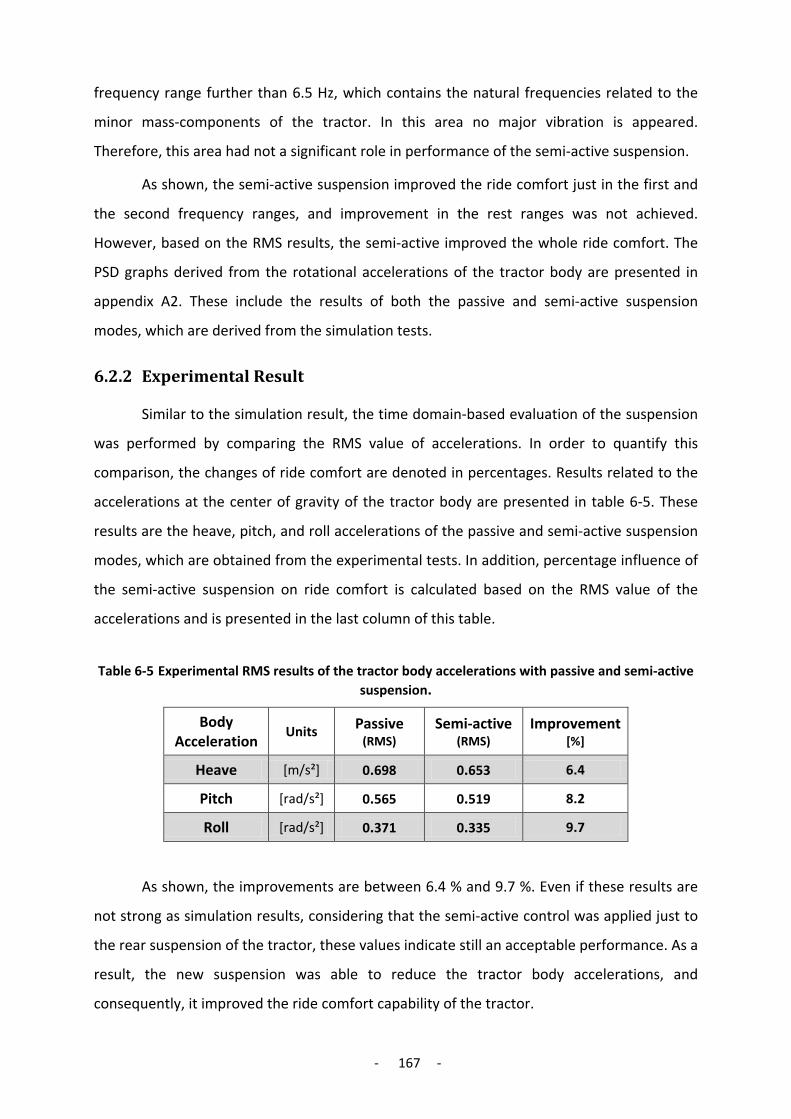
- 167 -

frequency range further than 6.5 Hz, which contains the natural frequencies related to the

minor mass-components of the tractor. In this area no major vibration is appeared.

Therefore, this area had not a significant role in performance of the semi-active suspension.

As shown, the semi-active suspension improved the ride comfort just in the first and

the second frequency ranges, and improvement in the rest ranges was not achieved.

However, based on the RMS results, the semi-active improved the whole ride comfort. The

PSD graphs derived from the rotational accelerations of the tractor body are presented in

appendix A2. These include the results of both the passive and semi-active suspension

modes, which are derived from the simulation tests.

6.2.2 Experimental Result

Similar to the simulation result, the time domain-based evaluation of the suspension

was performed by comparing the RMS value of accelerations. In order to quantify this

comparison, the changes of ride comfort are denoted in percentages. Results related to the

accelerations at the center of gravity of the tractor body are presented in table 6-5. These

results are the heave, pitch, and roll accelerations of the passive and semi-active suspension

modes, which are obtained from the experimental tests. In addition, percentage influence of

the semi-active suspension on ride comfort is calculated based on the RMS value of the

accelerations and is presented in the last column of this table.

Table 6-5 Experimental RMS results of the tractor body accelerations with passive and semi-active suspension.

Body Acceleration

Units Passive (RMS)

Semi-active (RMS)

Improvement [%]

Heave [m/s²] 0.698 0.653 6.4

Pitch [rad/s²] 0.565 0.519 8.2

Roll [rad/s²] 0.371 0.335 9.7

As shown, the improvements are between 6.4 % and 9.7 %. Even if these results are

not strong as simulation results, considering that the semi-active control was applied just to

the rear suspension of the tractor, these values indicate still an acceptable performance. As a

result, the new suspension was able to reduce the tractor body accelerations, and

consequently, it improved the ride comfort capability of the tractor.

- 168 -

Similar to simulation results, for experimental results, the frequency domain analysis

was considered in addition to the evaluation based on the time domain results. By frequency

domain analysis, the detailed operation of the semi-active system in different frequency

ranges was examined. This was performed based on the related PSD graphs. Figure 6-5

shows the PSD graphs derived from the vertical acceleration of the tractor body in the

passive and semi-active suspension modes, derived from the experimental tests.

Figure 6-5 Comparison between semi-active and passive frequency responses of the tractor body acceleration in the experimental test.

As seen, the frequency area of this graph is divided again into four ranges. The first

area is the frequency range from 0.5 to 2 Hz, containing the natural frequencies of the

tractor body (i.e. sprung mass). The peak of the curve in this area shows the natural

frequency related to the vertical movement of the tractor body. As shown, this frequency is

1.6 Hz. The natural frequencies of the body rotational movements were derived similarly in

the experimental tests. These data were presented in the validation section. As shown, the

best performance of the semi-active suspension in reduction of the acceleration occurs in

this area.

The second area is the frequency range of 2-4 Hz, located between the two areas of

the natural frequencies related to the sprung mass and unsprung mass. As mentioned, the

peak amplitude in this area appeared because of a friction effect. As shown the performance

IV

Semi-active

Passive II

NF.=1,6 Hz

I

III

- 169 -

of the semi-active suspension in this area is also considerable and reduces the acceleration

significantly.

The third area is the frequency range from 4 to 6.5 Hz. This area contains the natural

frequency of the wheels (i.e. unsprung masses). As shown, in this area, the acceleration level

was not reduced by the semi-active suspension. This happened because of two reasons.

First, the sky-hook control strategy in principle, concentrates on controlling the tractor body

vibration and not on controlling the wheel vibration, which is the source of the vibration

appearing in this frequency area. More discussion in this theme is presented in section of

“handling result”.

Secondly, a practicable rate was selected for the bandwidth of the controller with the

purpose of controlling the vibrations in the frequency range related to the tractor body

motions (i.e. first range). Therefore, as the frequency range goes far from the first range, the

control ability of the semi-active suspension reduced, and the suspension operation slanted

to a passive suspension. Despite the low performance of the semi-active suspension in the

third area, the overall performance of the system in controlling the vibration of the tractor

body was positive. This conclusion was obtained based on the related RMS results.

The fourth area is the frequency range further than 6.5 Hz, containing the natural

frequencies related to the minor mass-components of the tractor. In this area, no significant

vibration is observed. On the other hand, as explained, in this area the semi-active

suspension has no direct control. Therefore, this area is not considered important in

performance evaluation of the semi-active suspension.

Results of the experimental tests, similarly to the simulation results, revealed that the

semi-active suspension improved the ride comfort of the tractor. This improvement was

created particularly in the first and the second frequency ranges, and improvement in the

rest ranges was not achieved. However, the RMS results indicated that semi-active improved

the overall ride comfort. The PSD graphs derived from the rotational accelerations of the

tractor body are presented in appendix A3. These are the results of the experimental tests in

the passive and semi-active suspension modes.

6.3 Handling Evaluation

In order to evaluate the performance of the semi-active suspension, after ride

comfort, the handling capability of the tractor was investigated. As stated before, in order to

quantify the handling, vertical dynamic tire contact-force was measured. Similar to the ride

- 170 -

comfort study, by comparing the time domain and frequency domain results of the

suspension in the two modes of the passive and semi-active, the new suspension system was

evaluated. In this section, results of the simulation tests and experimental tests are

presented. In each part, the time domain results and frequency domain results are given.

These parts include the results of the two modes of the passive and semi-active suspension.

6.3.1 Simulation Result

Time domain analysis is performed based on the comparison of the RMS results of

the vertical dynamic tire force. The average of the RMS values derived from the dynamic tire

force of the tractor rear wheels are presented in table 6-6. These simulation results are given

for the two passive and semi-active suspension modes. In order to quantify this comparison,

the percentage improvement of ride comfort is given in the table as well.

Table 6-6 Simulation results of the dynamic tire force in the passive and semi-active suspension mode.

Dynamic Tire Force Passive Semi-active

Units

RMS 1267.6 1186.3 [N]

Improvement 6.4 [%]

As shown, the improvement of 6.4 % is gained. This result is considerable, because

the semi-active control was applied just to the rear suspension of the tractor and not to all

four wheels. On the other hand, since the skyhook control strategy is focused principally on

the vibration control of the vehicle body and not on the vibration control of the wheels.

Referring to the achieved result, the semi-active suspension was able to reduce the dynamic

tire force of the tractor significantly, and the handling capability of the tractor was improved

consequently.

The frequency-response results of the tractor body accelerations studied for ride

comfort investigation showed that in the third frequency range, which was related to the

vibration of the wheels, no positive performance by semi-active system was achieved. This

result was matched to the basic function of sky-hook strategy. However, the RMS results of

the dynamic tire force indicated that the new suspension had positive influence on the

handling capability of the tractor. In order to clarify this specious inconsistency, the

frequency-response of the dynamic tire force was studied.

- 171 -

The results of the frequency-based analysis of the dynamic tire force are presented as

the PSD graphs. Figure 6-6 shows one of these graphs derived from the dynamic tire force of

the tractor in passive and semi-active suspension modes, related to the simulation tests.

Figure 6-6 Comparison between semi-active and passive frequency responses of the dynamic tire force in the simulation test.

As seen, the frequency area of this graph is divided into three ranges. The first area is

the frequency range of 1 - 2 Hz, containing the natural frequencies of the tractor body (i.e.

sprung mass). As shown, the best performance of the semi-active suspension in reducing the

dynamic tire force was achieved in this area. The second area is the frequency range of 2 - 3

Hz, which is the area between two natural frequencies areas related to the sprung mass and

unsprung mass. As mentioned, the peak amplitude in this area appeared because of the

function of the friction model. As shown, the performance of the semi-active suspension in

this area was also considerable and reduced the amplitude of the dynamic tire force.

The third area is the frequency range from 4 to 6.5 Hz. This contains the natural

frequency of the wheels (i.e. unsprung masses). The peak of the curve in this area shows the

natural frequency related to the vertical motion of the tractor wheel that this frequency is

5.1 Hz. As shown, the dynamic tire force was not reduced by the semi-active in this area,

whereas based on the RMS results, the dynamic tire force was reduced, and handling was

improved.

The dynamic tire force is affected directly by the two factors of the vehicle body

vibration and wheel (i.e. unsprung mass) vibration (refer to section 5.3.2). Therefore, these

two factors were considered in order to investigate the influence of the semi-active

NF.=5,1 Hz

I

II III

Semi-active

Passive

- 172 -

suspension on the dynamic tire force. The PSD graphs related to the tractor body

accelerations showed that the semi-active suspension controlled notably the vibration of the

tractor body in the first frequency range. In order to examine the effect of the semi-active

suspension on the wheel vibration, the PSD graph derived from the vertical acceleration of

the wheels was studied.

Figure 6-7 shows the PSD graphs derived from the wheel acceleration in passive and

semi-active suspension modes, obtained from the simulation tests. In this graph two

frequency ranges is considered. The first one is the area including the natural frequencies of

the tractor body motions, and the second one is the area of the natural frequency related to

the wheel motion. As seen, in the first area, the role of the semi-active suspension in

reduction of the wheels acceleration is slightly positive. However, this effect in the third area

is significantly negative. This occurred because of the basics of sky-hook control strategy that

is focused on the vibration control of the body of a vehicle.

Figure 6-7 Comparison between semi-active and passive frequency responses of the unsprung mass (i.e. wheel) acceleration in the simulation test.

The negative effect on the wheel vibration was observable in the third frequency

range (i.e. wheel natural frequency area) of all the PSD graphs. However, this effect was

always small in comparison with the positive performance of the semi-active suspension on

the first frequency range (i.e. tractor body natural frequencies area). After looking at

equation 5-15 and considering that the mass of the tractor body is higher than unsprung

mass, it can be understood why the influence of the body vibration is greater than the factor

of the wheel vibration. This is the reason that the overall performance of the system in

Semi-active

Passive

- 173 -

controlling of the dynamic tire force was positive. This issue was observable especially in the

result of the dynamic tire force, as the dynamic tire force were improved significantly in spite

of the increase in the wheel acceleration. This was also approved in the RMS results of the

dynamic tire force.

6.3.2 Experimental Result

The average of the RMS values derived from the dynamic tire force of the rear wheels

are presented in table 6-7. These values are the results in the passive and semi-active

suspension modes and derived from the experimental tests. In order to quantify the

comparison of these two results, the percentage improvement is presented in the table as

well. This value indicates indeed the improvement of ride comfort, achieved by the new

semi-active suspension.

Table 6-7 Experimental results of the dynamic tire force in the passive and semi-active suspension mode.

Dynamic Tire Force Passive Semi-active

Units

RMS 1444.7 1381.8 [N]

Improvement 4.3 [%]

As shown, the improvement of 4.3 % is achieved. This result is not as strong as

simulation result, but it is still considerable, because as mentioned, the semi-active control

was employed just in the rear suspension of the tractor and not for the complete four

wheels. In addition, the skyhook control strategy is focused principally on the control of the

body vibration of a vehicle and not on the control of the wheels vibration. This result also

showed that in the experimental tests, the dynamic tire force of the tractor was reduced by

the semi-active suspension. Consequently, the handling capability of the tractor was

improved.

Performance of the semi-active suspension in reduction of the dynamic tire force in

different frequency ranges was studied by the frequency-response of the dynamic tire force.

Figure 6-8 shows the PSD graphs derived from the dynamic tire force of the tractor in the

passive and semi-active suspension modes, achieved from the experimental tests.

- 174 -

Figure 6-8 Comparison between semi-active and passive frequency responses of the dynamic tire force in the experimental test.

As seen, the frequency area of this graph is divided into three ranges. The first area is

the frequency range of 1 - 2 Hz, containing the natural frequencies of the tractor body (i.e.

sprung mass). As shown, the best performance of the semi-active suspension in reduction of

the dynamic tire force was gained in this area. The second area is the frequency range from 2

to 3.5 Hz. This area is located between two groups of the natural frequencies areas of the

sprung mass and natural frequencies areas of the unsprung masses. As mentioned, the peak

in this area appeared because of the friction-effect in the suspension elements. As shown,

performance of the semi-active suspension is also acceptable in this area, and the amplitude

of the dynamic tire force is reduced.

The third area is the frequency range from 4.5 to 7 Hz, which includes the natural

frequency of the wheels (i.e. unsprung masses). The peak of the curve in this area shows the

natural frequency related to the vertical motion of the tractor wheel. As shown, this

frequency is 5.4 Hz. In the third area, the dynamic tire force was not reduced by the semi-

active. However, the RMS results indicated that in general, the dynamic tire force was not

increased, but also a significant improvement in vehicle handling was achieved.

As mentioned, the dynamic tire force is affected directly by the two factors of the

body vibration and wheel vibration of a vehicle. The PSD graphs of the tractor body

accelerations showed that the semi-active suspension controlled remarkably the vibration of

the tractor body in the first frequency range. The PSD graphs of the tractor body

II

NF.=5,4 Hz

I

III

Semi-active

Passive

- 175 -

accelerations and dynamic tire force indicated that the effect of the semi-active suspension

on the reduction of the wheels acceleration in the third area was significantly negative. This

effect occurred because of the control logic of sky-hook strategy that is concentrated on the

vibration control of the body of a vehicle. However, using practicable sky-hook strategy

moderated this focus, and leads to improve the vibration control of the wheels partially as

well.

The semi-active suspension increased the wheels acceleration. This has just a slight

negative construction effect on the wheels. However, the indirect effect of this phenomenon

on the dynamic tire force is important, and it affects significantly on the handling of the

vehicle. This negative effect was recognizable in the third frequency range (i.e. wheel natural

frequency area) of all the PSD graphs. However, this effect was always small in comparison

with the positive performance of the semi-active suspension in the first frequency range (i.e.

tractor body natural frequencies area). This fact that the factor of the body vibration has

stronger effect than the wheel effect led to overall positive performance of the system,

particularly in reducing the dynamic tire force. This was also approved by the RMS results of

the dynamic tire force.

As whole, results of the experimental tests revealed similar to simulation results that

the semi-active suspension improved the handling capability as well as the ride comfort of

the tractor. This improvement was created particularly in the first frequency ranges, and

improvement in the third ranges was not achieved. Although, the RMS results indicated that

the semi-active reduced the total dynamic tire force of the tractor and so, improved the

handling capability.

6.4 Suspension Travel Evaluation

After the examination of ride comfort and handling as the dynamic parameters of the

tractor, a constructional parameter of suspension systems was considered in order to

evaluate the performance of the new suspension system. In design of a suspension system,

the available place between the vehicle chassis and each wheel used for suspension

elements is limited. Therefore, in design of a suspension system, this factor must be

considered. The related factor is the stroke of a suspension. Lower required stroke is

considered as an advantage in suspension design, because means that less suspension place

is needed. With conversion a passive suspension to an active suspension, this factor may be

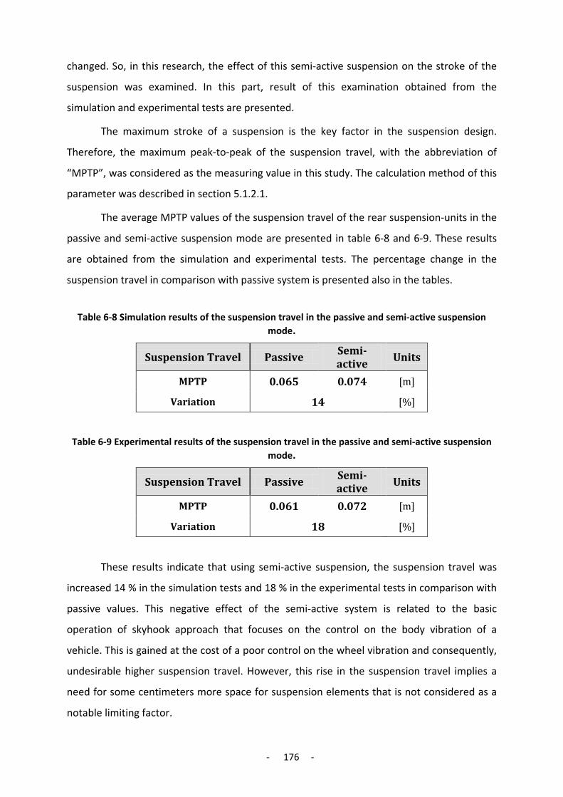
- 176 -

changed. So, in this research, the effect of this semi-active suspension on the stroke of the

suspension was examined. In this part, result of this examination obtained from the

simulation and experimental tests are presented.

The maximum stroke of a suspension is the key factor in the suspension design.

Therefore, the maximum peak-to-peak of the suspension travel, with the abbreviation of

“MPTP”, was considered as the measuring value in this study. The calculation method of this

parameter was described in section 5.1.2.1.

The average MPTP values of the suspension travel of the rear suspension-units in the

passive and semi-active suspension mode are presented in table 6-8 and 6-9. These results

are obtained from the simulation and experimental tests. The percentage change in the

suspension travel in comparison with passive system is presented also in the tables.

Table 6-8 Simulation results of the suspension travel in the passive and semi-active suspension mode.

Suspension Travel Passive Semi-active

Units

MPTP 0.065 0.074 [m]

Variation 14 [%]

Table 6-9 Experimental results of the suspension travel in the passive and semi-active suspension mode.

Suspension Travel Passive Semi-active

Units

MPTP 0.061 0.072 [m]

Variation 18 [%]

These results indicate that using semi-active suspension, the suspension travel was

increased 14 % in the simulation tests and 18 % in the experimental tests in comparison with

passive values. This negative effect of the semi-active system is related to the basic

operation of skyhook approach that focuses on the control on the body vibration of a

vehicle. This is gained at the cost of a poor control on the wheel vibration and consequently,

undesirable higher suspension travel. However, this rise in the suspension travel implies a

need for some centimeters more space for suspension elements that is not considered as a

notable limiting factor.

- 177 -

6.5 Result Summary

In order to evaluate the semi-active suspension, two groups of the simulation tests

and experimental tests with a similar plan were performed. In each group, three series of

tests with the three different input tests were used. Evaluation of the new suspension was

done by comparing the passive and semi-active suspension modes. Therefore, each test was

performed once in the passive mode and then, in the semi-active mode. The achieved data

from these tests in the two suspension modes were analyzed in order to derive the

amplitude and frequency based results of the system. These results were presented in the

RMS values and the frequency domain graphs. The frequency-domain graphs were used in

order to investigate the vibration characteristic of the suspension system in different

frequency ranges of the system bandwidth.

Vibration control of the tractor body, particularly in the area of the body natural

frequencies, was considered as priority motive for using an active suspension for tractors.

The control strategy used for the semi-active suspension was selected considering this

concern. In evaluation of the semi-active suspension, the ride comfort capability of the

tractor was considered as the first criterion. For this purpose, accelerations of the tractor

body were measured, and the influence of the new suspension system on the ride comfort

capability of the tractor was evaluated by comparing the results of the passive and semi-

active suspension modes. The following charts show the summary results related to the

tractor body accelerations, acquired from the simulation and experimental tests.

Figure 6-9 Comparison between RMS results of the tractor body accelerations in the simulation tests.

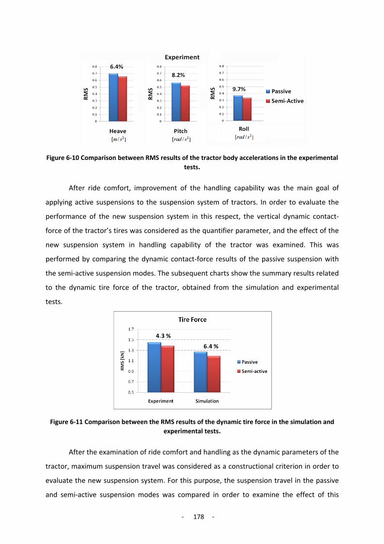
- 178 -

Figure 6-10 Comparison between RMS results of the tractor body accelerations in the experimental tests.

After ride comfort, improvement of the handling capability was the main goal of

applying active suspensions to the suspension system of tractors. In order to evaluate the

performance of the new suspension system in this respect, the vertical dynamic contact-

force of the tractor’s tires was considered as the quantifier parameter, and the effect of the

new suspension system in handling capability of the tractor was examined. This was

performed by comparing the dynamic contact-force results of the passive suspension with

the semi-active suspension modes. The subsequent charts show the summary results related

to the dynamic tire force of the tractor, obtained from the simulation and experimental

tests.

Figure 6-11 Comparison between the RMS results of the dynamic tire force in the simulation and experimental tests.

After the examination of ride comfort and handling as the dynamic parameters of the

tractor, maximum suspension travel was considered as a constructional criterion in order to

evaluate the new suspension system. For this purpose, the suspension travel in the passive

and semi-active suspension modes was compared in order to examine the effect of this

4.3 %

6.4 %

- 179 -

semi-active suspension on the stroke of the suspension. The following charts show the

summary results related to the maximum suspension, acquired from the simulation and

experimental tests.

Figure 6-12 Comparison between the MPTP results of the suspension travel in the simulation and experimental tests.

Table 6-10 presents the result of a comparative study with the intention of evaluating

the performance of the semi-active suspension in the simulation tests and experimental

tests. In this table, the whole measured parameters are considered. A view of these results

reveals that the simulation results in comparison with the experimental results indicated

always a better performance for the new suspension system. In addition, after referring to

the RMS results, it was realized that the simulation results had lower magnitude than

corresponding experimental results.

Table 6-10 Difference in performance of the semi-active suspension in the simulation and experimental tests.

Parameter Mode Improvement (%)

Simulation Experiment

Body Acceleration Heave 9.4 6.4

Body Acceleration Pitch 10.7 8.2

Body Acceleration Roll 13.3 9.7

Dynamic Tire Force 6.1 4.3

Suspension Travel 14 18

14% 18%

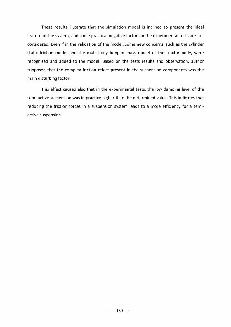
- 180 -

These results illustrate that the simulation model is inclined to present the ideal

feature of the system, and some practical negative factors in the experimental tests are not

considered. Even if in the validation of the model, some new concerns, such as the cylinder

static friction model and the mulit-body lumped mass model of the tractor body, were

recognized and added to the model. Based on the tests results and observation, author

supposed that the complex friction effect present in the suspension components was the

main disturbing factor.

This effect caused also that in the experimental tests, the low damping level of the

semi-active suspension was in practice higher than the determined value. This indicates that

reducing the friction forces in a suspension system leads to a more efficiency for a semi-

active suspension.

- 181 -

Chapter 7

7 Conclusion

This chapter is intended to summarize the work, which was done for this thesis, and to

present the conclusions, which were achieved from this study. The chapter is concluded with

several suggestions for future research in order to extend this work.

7.1 Summary and Conclusions

Main objective of this research was to improve suspension performance of

agricultural tractors by using a proper active suspension system. In order to accomplish this

objective, the background of the research was studied initially. This study leads to choose a

proper active suspension system for agricultural tractors. For evaluation of this new

suspension system, two approaches of the computer simulation testing and experimental

testing were used.

In order to perform the evaluation tests, the design and plan of the simulation and

experimental tests were determined. The output of the tests was the acceleration data of

the tractor body and wheel. These data were analyzed in order to obtain the time and

frequency domain results of the vibration modes. These results were used in order to

evaluate the ride comfort and handling ability of the tractor. Based on the investigations

done for this thesis, the following conclusions are drawn:

• Idea of active suspension for agricultural tractors. In this research, available options

for an active system for the chassis suspension of agricultural tractors were studied.

As the best choice, a semi-active suspension with the control strategy of “on-off

skyhook” was selected.

• Modeling of the new suspension system. For this purpose, a computer model of the

tractor counting the suspension model, using MATLAB-Simulink program, was built.

The model consisted of the test-tractor model and the semi-active suspension model.

The semi-active suspension model was composed of three sub-model models:

controller, actuator, and sensor models.

- 182 -

• Development of the prototype of the new suspension system. In order to perform

the practical evaluation of this new system, the full suspension test-tractor of TU-Trac

with hydro-pneumatic rear suspension was determined. A prototype of the new

suspension system was developed and then, on the rear axle suspension of the test-

tractor was installed. The prototype consisted of three parts: set of the sensors,

hydraulic actuators, and electronic controller.

• Design of the tests. In order to evaluate the performance of the new suspension by

simulation and experimental testing, design and plan of the tests were determined.

The suspension system was excited by the three set of impulse inputs, which were

applied to the four tractor’s wheels. Each test was performed in the two suspension

modes of the passive and semi-active.

• Operation of a suspension test rig for performing the tests. In order to perform an

accurate test in the experimental tests, the suspension test rig at the TU Berlin -

Department Machinery System Design was employed. This test rig used to simulate

three different road inputs in order to excite the suspension system in order to

perform the evaluation tests.

• Model validation. The overall model was validated by comparing the simulation

results with experimental results. In the highest deviations, there was 77 %

correlation between the simulation RMS results and the experimental results,

indicating good validity of the model. Referring to the PSD results, frequency

response of the simulation results had acceptable correlation with experimental

results. These results from the validation indicated that the simulation model was

able to simulate the dynamic behavior of the suspension system of tractors and

estimate the vibration transmission accurately.

• Examination of the tractor ride comfort. The comparison between passive and semi-

active results in the simulation and experimental tests demonstrated that the

accelerations of the tractor body were reduced until 13 % in the simulation tests and

10% in the experimental test by using the new suspension system. These results

implied that a significant improvement in the ride comfort of the tractor was

achieved.

• Examination of the tractor handling. The comparison between passive and semi-

active results in the simulation and experimental tests indicated that the average of

- 183 -

the tractor dynamic tire force was reduced until 6.5 % in the simulation tests and 4.5

% in the experimental tests by using the new suspension system. These results

implied that an acceptable improvement in tractor handling was achieved.

• Examination of the suspension travel. The results indicated that using the semi-active

suspension was increased 14 % the suspension travel in the simulation test and 18 %

in the experimental test. Considering the overall suspension stroke, this increase in

the suspension travel indicated a need for some centimeters more space for

suspension elements that was not considered as a notable limiting factor.

7.2 Recommendations

The specific recommendations that can be expanded on this investigation and follow it are

stated as:

• Use of a hybrid active suspension for the agricultural tractors. These vehicles drive on

the different road conditions such as asphalt street and field way. They perform

different operations such as fast-duty fieldwork, heavy-duty fieldwork, and stationary

work. A typical semi-active suspension is not capable to cover all these different

conditions. By using an adaptive suspension together with the semi-active

suspension, the suspension parameters can be changed largely after a major change

in the working condition, and then, the semi-active suspension can provide an

efficient performance for the agricultural tractor in the different working conditions.

• An idea for the adaptive suspension system is the use of the driver command sensors

for the semi-active suspension. This can be performed by involving these data in the

control loop in order to provide prediction of the maneuver inputs entering to the

suspension system. These sensors could install on the break pedal, gas pedal, and

steering wheel in order to measure the break, accelerating, and turning commands.

Another similar idea is to analyze the frequency response of the acceleration on the

wheels as the input of the adaptive control in order to realize general road

excitations. In addition, similar to the research of (Hansson P. , 1996), the preview

sensors installing on the front axle can be used in order to predict the road inputs

entering to the rear axle. This extra sensory information can be added to the control

loop of the semi-active suspension system as is shown in figure 7-1.

- 184 -

Figure 7-1 Driver command sensors for the semi-active control loop in order to provide a more efficient control.

• In extreme driving conditions or in station work, using the chassis suspension system

for tractor may lead to an instability situation. Then, a blockage mode can be useful

for the suspension system of tractors. In this research, in the hydro-pneumatic

suspension the double-acting cylinders were used.

In order to apply the suspension blockage mode to each unit, two hydraulic

valves can be simply added to the hydro-pneumatic circuit, between the

accumulators and cylinder in both sides of the double-acting cylinders. As these

valves are off, the cylinder inlets are closed, and the cylinder is blocked. Because of

the position of these valves between the accumulators and cylinder, the throttling

effect of them must be considered in the design of the semi-active suspension system

explained in section 3.2.2.

• Different damping ratio can be evaluated for the high and low levels of damping

related to the on-off sky-hook strategy.

• The influence of the semi-active controller bandwidth on the suspension

performance can be investigated.

• In addition to the rear axle suspension, the semi-active suspension can be applied to

the front axle suspension of the tractor, and then, performance of a full semi-active

suspension for agricultural tractors can be evaluated.

• In addition to on-off skyhook, efficiency of other control strategies can be examined

for the semi-active suspension of the tractor. Some of these methods were

mentioned in section 2.3.

Feedback Loop

Feedforward

Loop

Sensors

Controller Actuator Tractor

Excitation Sensors

- 185 -

• Using the validated model as virtual prototype for developing investigation. This

includes naturally all the recommended objects here.

• The full tractor model, which was created in this research, can be improved and

developed as follow:

- A more accurate model can be built for the tractor body by considering the

elasticity of the masses of the body and the connections among them.

- A more accurate tire model can be built considering tire pressure and other

tire parameters. In this research, it was indicated that the model of the tires

have significant influence on the simulation accuracy.

- Friction effect can be considered in modeling of more suspension

components.

- Model of the sensors can be built considering possible happening errors.

• The benefits of MR dampers can be evaluated for the actuator of a semi-active

suspension. The main advantage of these dampers is its very low response delay that

can increase the bandwidth of the control system.

• There is friction effect in the different elements of a semi-active suspension. The

effect of these frictions on the suspension performance can be investigated.

• In this study, a test rig was used in order to evaluate the active suspension system.

Since this study was the first step of the examination of the new suspension, the test

rig was used to eliminate the different errors occurring during the typical field tests.

As the next step, the tests can be performed by driving the test-tractor on the

different types of roads. This can be performed by simulation using a road model

before. For this purpose, a challenging point is the measurement of the absolute

velocity that is needed for skyhook control strategy. This subject should be studied as

well to achieve to a sure method.

- 186 -

References

Abd El-Tawwab, A. M. (1997). Twin-Accumulator Suspension System. Warrendale: Society of Automotive Engineers: SAE Technica l paper no.970384.

Adams, B. T. (2002). Central Tire Inflation For Agricultural Vehicles. Ph.D. Dissertation, University of Illinois, USA.

Ahmadian, M. (1997). Semiactive Control of Multiple Degree of Freedom Systems. Proceedings of Design Engineering Technical Conferences.

Ahmadian, M., & Pare, C. A. (2000). A Quarter-Car Experimental Analysis of Alternative Semiactive Control Methods. Journal of Intelligent Material Systems and Structures, 11 (8), 604-612.

Al-Holou, N., Joo, D. S., & Shaout, A. (1996). The Development of Fuzzy Logic Based Controller for Semi-Active Suspension System. Proceedings of the 37th Midwest Symposium on Circuits and Systems, (pp. 1373-1376).

Baillie, A. S. (1999). Development of a Fuzzy Logic Controller For an Active Suspension of an Off-Road Vehicle Fitted with Terrain Preview. Master Thesis, Royal Military College of Canada, Kingston, Ontario.

Barak, P. (1989). Design and Evaluation of Adjustable Automobile Suspension. SAE Paper 890089 .

Barak, P. (1991). Magic Numbers in Design of Suspension for Passenger Cars. SAE Technical Papers Series, n. 878, pp.53-88.

Barr, A., & Ray, J. (1996). Control of an active suspension using fuzzy logic. Proceedings of the Fifth IEEE International Conference on Fuzzy Systems, 1, pp. 42-48.

Bastow, D. (1987). Car Suspension and Handling. Pentech Press Limited, London.

Bauer, W. (2007). Hydropneumatische Federungssysteme. Springer.

Blundell, M. (1999). The Modelling and Simulation of Vehicle Handling Part 3: Tire Modelling. Journal of Multi-body Dynamics, 214 (1), 1-32.

Boileau, P.-E., & Rakheja, S. (1990). Vibration attenuation performance of suspension seats for off-road forestry vehicles. International Journal of Industrial Ergonomics, 5, 275-291.

Boonchanta, P. (1982). Comparisons of Active, Passive, and Semiactive Suspensions for Ground Vehicles. Ph. D. Dissertation, University of California, Davis, CA, USA.

Burton, A., Truscott, A., & Wellstead, P. (1995). Analysis, Modelling and Control of an Advanced Automotive Self-Levelling Suspension System. IEE Proc.-Control Theory Appl., 142 (2), 129-139.

Carter, A. K. (1998). Transient Motion Control of Passive and Semiactive Damping for Vehicle Suspensions. Master Thesis, Virginia Tech., Blacksburg, Virginia, USA.

- 187 -

Chalasani, R. (Dec.1986). Ride Performance Potential of Active Suspension Systems-Part I:Simplified Analysis Based on a Quarter-Car Model. Proceedings of 1986 ASME Winter Annual Meeting. Los Angeles, CA.

Chalasani, R. (1986). Ride Performance Potential of Active Suspension Systens-Part II: Comprehensive Analysis Based on a Full-Car Model. ASME Symposium on Simulation and Control of Ground Vehicles and Transportation Systems, 80 (2), 187-204.

Chaudhary, S. (1998). Ride a Roll Performance Analysis of a Vehicle with spring Loaded Interconnected Hydro-Pneumatic Suspension. Master Thesis, Concordia University, Montreal, Quebec, Canada.

Claar, P., Sheth, P., Marley, S., & Buchele, W. (1980). Agricultural tractor chassis suspension system for improved ride comfort. ASAE Paper, 80, 1565.

Class. (2006). Retrieved 2006, from www.claas.de

Crolla, D. A., & Abdel-Hady, M. B. (1991). Semi-Active Suspension Control for a Full Vehicle Model. SAE (Society of Automotive Engineers) Transactions, 100 (6), 1660-1666.

Deakin, A., Crolla, D., & Shovlin, A. (1997). Power Consumption in Ride of a Combat Support Vehicle Slow-Active Suspension. SAE Special Publication, vol.38.

Deutz. (2006). Retrieved June 2006, from Deutz Tractors: http://www.deutz-fahr.de

Donahue, M. D. (1998). Implementation of an Active Suspension, Preview Controller for Improved Ride Comfort. Master Thesis, University of California, Berkeley, USA.

Efatpenah, K., Beno, J. H., & Nichols, J. H. (2000). Energy Requirements of a Passive and an Electromechanical Active Suspension System. Vehicle System Dynamics, 34 (6), 437-458.

Elmadany, E. M., & Abduljabbar, Z. (1999). Linear Quadratic Gaussian Control of a Quarter-Car Suspension. Vehicle System Dynamics, 32 (6), 479-497.

Eulenbach, D. (2003). Stand und Entwicklungstrends hydropneumatischer Niveauregelsysteme. Haus der Technik, Essen, Germany.

FASTRAC. (2007). JCB FASTRAC. Retrieved April 2007, from http://www.jcb.com/products/MachineOverview.aspx

Festo. (2003). Hydraulics Basic Level. Denkendorf, Germany: Festo.

Fodor, M., & Redfield, R. (1995). Resistance Control, Semi-Active Damping Performance. Advanced Automotive Technologies American Society of Mechanical Engineers, Dynamic Systems and Control Division, 161-169.

Giliomee, C. L. (2003). Analysis of a Four State Switchable Hydro-Pneumatic Spring and Damper System. Master Thesis, University of Pretoria, South Africa.

Gillespie, T. (1992). Fundamentals of Vehicle Dynamics. USA: SAE.

- 188 -

Giua, A., Savastano, A., Seatzu, C., & Usai, G. (1998). Approximation of an Optimal Gain Switching Active Law with a Semiactive Suspension. IEEE Conference on Control Applications- Proceedings , Piscataway, NJ,USA, 248-252.

Goehlich, H. (1984). The Development of Tractors and Other Agricultural Vehicles. J. agric. Engng Res., 29, 3-16.

Göhlich, H., Hauck, M., & von Holst, C. (1999). Fahrdynamik – Fahrsicherheit – Fahrerplatz. Jahrbuch Agrartechnik. 11, pp. 61 – 69. Landwirtschaftsverlag Münster, 1999.

Goncalves, F. (2001). Dynamic Analysis of Semiactive Control Techniques for Vehicle Applications. Master Thesis, Virginia Tech., Blacksburg, Virginia, USA.

Gunston, T. (2000). The Definition of Suitable Input Motions for Testing Suspension Seat End-stop Impact Performance. 34th meeting of the U.K. Group on Human Response to Vibration, (pp. 127-137).

Hansen, M. R., & Andersen, T. O. (2003). Active Damping of Oscillations in Off Road Vehicles. 8th Scandinavian Intl Conference on Fluid Power, 2, 1073-1085.

Hansson, P. A. (1995). Optimization of Agricultural Tractor Cab Suspension Using the Evolution Method. Computers and Electronics in Agriculture, 12, 35-49.

Hansson, P. (1995). Optimization of Agricultural Tractor Cab Suspension Using the Evolution Method. Computers and Electronics in Agriculture, 12, 35-49.

Hansson, P. (1996). Rear axle suspensions with controlled damping on agricultural tractors. Computers and Electronics in Agriculture, 15, 123-147.

Hauck, M. (2001). Geregelte Dämpfung für Traktor-Fahrersitze. Ph.D. Dissertation, TU-Berlin, Germany.

Heo, S., Park, K., & Hwang, S. (2000). Performance and Design Consideration for Continuously Controlled Semi-Active Suspension Systems. International Journal of Vehicle Design, 23 (3), 376-389.

Hilmes, R. (1982). Dreissig Jahre Kampfpanzerentwicklung (1950-1980). Soldat und Technik 6, 324-329.

Hilton, D. J., & Moran, P. (1975). Experiments in Improving Tractor Operator Ride by Means of a Cab Suspension. J. agric. Engng Res., 20 (4), 433-448.

Hoppe, U. (2006). Einfluss der Hinterachsfederung auf die Fahrdynamik von Traktoren. Ph.D. Dissertation, TU-Berlin, Germany.

Hoppe-, U., & Meyer, H. J. (2005). Entwicklung und Realisierung eines vollgefederten Traktors. Tagung Landtechnik 2005, VDI Verlag, Düsseldorf .

Hoppe-01, U. (2004). Stand der Technik und aktuelle Entwicklungen bei der Traktorfederung. Neue Landwirtschaft, 5, 43-46.

Horton, D., & Crolla, D. (1984). Designing Off-Road Vehicles with Good Ride Behavior. Proceedings of the 8th International Conference of the ISTVS. 1, pp. 171-184. Amsterdam, The Netherlands: Elsevier Science.

- 189 -

Hyvärinen, J. P. (2004). The Improvement of Full Vehicle Semi-active Suspension Through Kinematical Model. Ph.D. Dissertation, University of Oulu, Finland.

ISO2631. (1974). Mechanical Vibration and Shock - Evaluation of Human Exposure to Whole Body Vibrations. Part 1: General Requirement, ISO 2631-1, The International Organisation for Standardisation.

ISO5008. (1979). Agricultural wheeled tractors and field machinery - Measurement of whole-body vibration of the operator. The International Organisation for Standardisation.

Jalili, N. (2002). A Comparative Study and Analysis of Semi-Active Vibration-Control Systems. Journal of Vibration and Acoustics, 124, 593-605.

Jamei, M. (2002). Symbiotic Rvolution-Based Design of Fuzzy Inference System with Application to Active Suspension system. Ph.D. Dissertation, University of Sheffield, Great Britain.

Jonh.Deere. (2005). Retrieved April 2005, from John Deere Tractors: http://www.deere.com/en_US/ProductCatalog

Kaczmarek, R. (1984). Central Tire Inflaiton Systems (CTIS) – A means to enhance vehicle mobility. Proceedings of the 8th International Conference of the ISTVS. 3, pp. 1255-1271. Amsterdam, The Netherlands: Elsevier Science.

Kaplick, C. (1995). Verifikation und Bewertung fahrdynamischer Traktor Simulationsmodelle. Ph.D. Dissertation, TU-Berlin, Germany.

Kaplick, C. (1995). Verifikation und Bewertung fahrdynamischer Traktor Simulationsmodelle. Ph.D. Dissertation, TU-Berlin, Germany.

Karnopp, D., & Heess, G. (1991). Electronically Controllable Vehicle Suspension. Vehicle System Dynamics 20, 207-217.

Karnopp, D., & Margolis, D. (1984). Adaptive suspension concept for road vehicles. Vehicle System Dynamics, 13 (3), 145-160.

Karnopp, D., Crosby, M. J., & Harwood, R. A. (1974). Vibration Control Using Semi-Active Force Generators. ASME Journal of Engineering for Industry, 96 (2), 619-626.

Kauß, W. (1981). Aktive, hydraulische Schwingungsisolierung des Fahrerplatzes ungefederter, geländegängiger Fahrzeuge. Ph.D. Dissertation, TU-Berlin, Germany.

Kauss, W., & Weigelt, H. (1980). Die gefederte Traktorkabine - verbesserter Schwingungsschutz und Fahrkomfort. Landtechnik, 9, 396-401.

Kising, A. (1988). A Dynamische Eigenschaften von Traktor-Reifen. Ph.D. Dissertation, TU-Berlin, Germany.

Langlois, R., Anderson, R., & Hanna, D. (1991). Implementing Preview Control on an Off-Road Vehicle with Active Suspension. Proceedings 12th IAVSD Symposium on the Dynamics of Vehicles. France, Lyon, Swets and Zeitlinger.

- 190 -

Lehmann, K. (2004). Analyse von Niveauregelungssystemen für Traktoren. Diplomarbeit, TU-Berlin, Germany.

Lehtonen, T., & Juhala, M. (2006). Predicting the ride behaviour of a suspended agricultural tractor. International Journal of Vehicle Systems Modelling and Testing, 1 (1-2), 131-142.

Lizell, M. (1990). Dynamic levelling for ground vehicles. Ph.D. Dissertation, Norstedts tryckeri, Stockholm, Sweden.

Mäkelä, K. (1999). Characterization and performance of electrorheological fluids based on pine oils. VTT publications 385, Espoo.

Margolis, D. (1982). The Response of Active and Semiactive Suspensions to Realistic Feedback Signals. Vehicle System Dynamics, 11 (5-6), 267-282.

Margolis, D., & Nobles, C. M. (1991). Semi-Active Heave and Roll Control for Large Off-Road Vehicles. SAE Special Publications. n 892, 25-34.

Marsili, A., Ragni, L., Santoro, G., & Servadio, G. (2002). Innovative Systems to Reduce Vibrations on Agricultural Tractors: Comparative Analysis of Acceleration Transmitted Through the Driving Seat. Biosystems Engineering, 81 (1), 35-47.

Masi, J. W. (2001). Effect of Control Techniques on the Performance of Semiactive Dampers. Masters Thesis, Virginia Polytechnic Institute, Blacksburg, Virginia.

McLellan, N. (1998). On the Development of a Real-Time Embedded Digital Controller for Heavy Truck Semiactive Suspensions. Master Thesis, Virginia Tech., Blacksburg, Virginia, USA.

McMichael, S. C. (1981). The Simulation and Spectral Analysis of A Motorcycle Model with a Semiactive On-Off rear Shock Absorber. Ph.D.Dissertation, University of California, Davis, CA, USA.

Meller, T. (1987). Self-Energizing Hydropneumatic Levelling System. SAE Technical paper no 780052, Warrendale: Society of Automotive Engineers.

Meyer, H. J. (2005). Ölhydraulik und Pneumatik II. Vorlesungsumdruck, TU-Berlin, Germany.

Meyer, H. (2006). Konstruktion von Maschinensystemen. Vorlesungsskript, TU-Berlin.

Meyer, H. (2004). Mobile Arbeitsmaschinen. Vorlesungsskript, TU-Berlin, Germany.

Meyer, H. (2004). Schwingungsentkopplung bei Landmaschinen. Landtechnik, 1, 24–25.

Miller, L. (1988). Tuning Passive, Semi-Active, and Fully Active Suspension Systems. Proceedings of the 27th IEEE Conference on Decision and Control, 3, pp. 2047 - 2053.

Mitschke, M. (1984). Dynamik der Kraftfahrzeuge (2 ed., Vol. B). Berlin: Springer.

Müller, N. (2001). Einfluss der Hinterachsfederung auf die Fahrsicherheit und den Fahrkomfort von Ackserschleppern. Forschungsbericht, TU-Berlin, Germany.

New-Holland. (2005). Retrieved March 2005, from New Holland Tractors: http://www.newholland.com/home.asp

- 191 -

Nobles, C. M., & Miller, L. R. (1985). The Design and Development of a Semi-Active Suspension for a Military Tank. SAE Technical Paper Series No. 881133 .

Paré, C. A. (1998). Experimental Evaluation of Semiactive Magneto-Rheological Suspensions for Passenger Vehicles. Master Thesis, Faculty of the Virginia Polytechnic Institute, Blacksburg, Virginia.

Pickel, P. (1993). Simulation fahrdynamischer Eigenschaften von Traktoren. Ph.D. Dissertation, TU-Berlin, Germany.

Pickel, P., Kaplick, P., & Göhlich, H. (1990). Welche Chancen haben gefederte Traktoren? Landtechnik, 10 ( 90), 363-366.

Profi. (2007). Sicherer und Komfortabler Arbeiten mit Einem Gefederten Schlepper. Profi Test (Tractors Profi and Farm Machinery), 2/99, 10-18.

Rhenius, K. T. (1983). Erhöhte Arbeitsgeschwindigkeiten und Schleppertechnik:Wo liegen die Grenzen? Landtechnik, 38 (11), 466-469.

Rill, G., Slag, D., & Wilks, E. (1992). Improvement of Dynamic Wheel Loads and Ride Quality of Heavy Agricultural Tractors by Suspending Front Axls. Heavy Vehicle and Roads-Technology,Safety and Policy, Telford, London, 116-121.

Rolvag, T. (2004). Design and optimization of Suspension Systems and Components. Norwegian University of Science and Technology NTNU.

SAE. (1992). Measurement of Whole Body Vibration of the Seated Operator of Off-Highway Work Machines. SAE J1013, Society of Automotive Engineers, Warrendale, PA.

Sampson, D. J. (2000). Active Roll Control of Articulated Heavy Vehicles. Ph.D. Dissertation, Cambridge University, Cambridge, UK.

Satoh, M., Fukushima, N., Akatsu, Y., Fujimura, I., & Fukuyama, K. (1990). An Active Suspension Employing an Electrohydraulic Pressure Control System. Proceedings of the 29th IEEE Conference on Decision and Control.

Scarlett, A. J., Price, J. S., & Stayner, R. M. (2007). Whole-Body Vibration: Evaluation of Emission and Exposure Levels Arising from Agricultural Tractors. Journal of terramechanics, 44 (1), 65-73.

Siekmann, H. (2003). Strömungslehre für den Maschinenbau. Springer.

Simon, D. (2001). An Investigation of the Effectiveness of Skyhook Suspensions for Controlling Roll Dynamics of Sport Utility Vehicles Using Magneto-Rheological Dampers. Ph.D. Dissertation, Virginia Tech., Blacksburg, Virginia, USA.

Soliman, A., & Crolla, D. A. (1996). Preview control of a semi-active suspension system. International Journal of Vehicle Design, 17 (4), 384-397.

Standards. (2004). Vehicle Standards Bulletin VSB 11. Department of Transport and Regional Services. Canberra: Vehicle Safety Standards.

Stayner, R. M., & Bean, A. G. Tractor Ride Investigations. A survey of vibration experienced by drivers during field work. Natn. Inst. agric. Engng Dept. Note DN/E/578/1445.

- 192 -

Stein, G., & Ballo, I. (1991). Active Vibration Control System for the Driver’s Seat for Off-road Vehicles. Vehicle System Dynamics, 57-78.

Suggs, C., & Huang, B. (1969). Tractor Cab Suspension Design and Scale Model Simulation. Trans.ASAE, 12, 283-289.

Thiebes, P. (2006). Fahrdynamik eines vollgefederten Traktors Hybride Modellierung, Simulationsvalidierung. Diplomarbeit, TU-Berlin, Germany.

Thiebes, P., Müller, P., & Gericke, K. (2005). Konstruktion und Analyse eines Traktorrahmens zur Aufnahme einer gefederten Hinterachse. Projektarbeit, TU-Berlin, Germany.

Thoresson, M. J. (2003). Mathematical Optimisation of the Suspension System of an Off-Road Vehicle for Ride Comfort and Handling. Master Thesis, University of Pretoria, Pretoria.

Titli, A., & Roukieh, S. (1995). Design of Active and Semi-Active Automotive Suspension Using Fuzzy Logic. Proceedings of the 12th Triennial World Congress of the International Federation of Automatic Control, 3, pp. 73-77. Pegamon, Oxford, UK.

Ulrich, A. (1983). Untersuchung zur Fahrdynamik von Traktoren mit und ohne Anbaugerät. Ph.D. Dissertation, TU-Berlin, Germany.

Uriarte, C. (2007). Studie verschiedener Regelstrategien für die adaptive Dämpfung einer Kabinenfederung. Analytische Studienarbeit, TU-Berlin, Germany.

Valášek, M., Novak, M., Sika, Z., & Vaculin, O. (1997). Extended ground-hook – new concept of semiactive active control of truck’s suspension. Vehicle system dynamics, 27 (5-6), 289-303.

Valtra. (2005). Retrieved March 2005, from Valtra Tractors: http://www.valtra.com

Vaughan, J. E. (2004). Active and Semi-Active Control to Counter Vehicle Payload Variation. Master Thesis, Georgia Institute of Technology, USA.

Vessonen, I., & Järviluoma, M. (2001). Simulation Based Design of Mobile Machine Vibration Control and Active Cabin Suspension Prototype. VTT Symposium 209, (pp. 121-139). Espoo, Finland.

Von Holst, C. (2000). Vergleich von Reifenmodellen zur Simulation der Fahrdynamik von Traktoren. Ph.D. Dissertation, TU-Berlin, Germany.

Weigelt, H. (1987). Schwingungseigenschaften Vorderachsgefederter Landwirtschaftlicher Traktoren. Ph.D. Dissertation, TU-Berlin, Germany.

Williams, R. A. (1994). Electronically Controlled Automotive Suspensions. Computing & Control Egineering Journal, 143-148.

Yi, K., & Hedrick, K. (1993). Dynamic Tire Force Control by Semiactive Suspensions. Journal of Dynamic Systems Measurement & Control-Transactions of the ASME, 115 (3), 465-474.

Zadeh, L. A. (1965). “Fuzzy Sets,”. Information and Control, 8, 338-353.

Ziemer, R. E., Tranter, W. H., & Fannin, D. R. (1998). Signals & Systems. New Jersey: Prentice Hall.

- 193 -

Appendices

Appendix A: Rest PSD Graphs

A.1: Passive, Experiment-Simulation

Figure A-1: Comparison between simulation and experimental frequency responses of the tractor body “pitch” acceleration.

- 194 -

Figure A-2: Comparison between simulation and experimental frequency responses of the tractor body “roll” acceleration.

Figure A-3: Comparison between simulation and experimental frequency responses of the dynamic tire force.

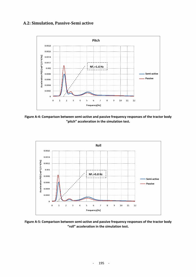
- 195 -

A.2: Simulation, Passive-Semi active

Figure A-4: Comparison between semi-active and passive frequency responses of the tractor body “pitch” acceleration in the simulation test.

Figure A-5: Comparison between semi-active and passive frequency responses of the tractor body “roll” acceleration in the simulation test.

NF.=0.8 Hz

NF.=1.6 Hz

Semi-active

Passive

Semi-active

Passive

- 196 -

A.3: Experiment, Passive-Semi active

Figure A-6: Comparison between semi-active and passive frequency responses of the tractor body “pitch” acceleration in the experimental test.

Figure A-7: Comparison between semi-active and passive frequency responses of the tractor body “roll” acceleration in the experimental test.

NF.=1.7 Hz

NF.=1 Hz

Semi-active Passive

Semi-active Passive

Semi-active Passive

- 197 -

Appendix B: Suspension Test Rig

Technical data of the Full Suspension Test Rig

1- Hydraulic Cylinder

80 𝑚𝑚𝑚𝑚 Piston diameter

60 𝑚𝑚𝑚𝑚 Piston-rod diameter

80 𝑚𝑚𝑚𝑚 Max. stroke

±90 𝑚𝑚𝑚𝑚 Max. piston speed

2- Hydraulic Pumps

2,45 𝑘𝑘𝑘𝑘 Power

280 𝑏𝑏𝑟𝑟𝑟𝑟 Pressure

180 𝑓𝑓/𝑚𝑚𝑝𝑝𝑛𝑛 Rate of flow

3- Valves*

100 𝑓𝑓/𝑚𝑚𝑝𝑝𝑛𝑛 Nominal rate of flow at ∆𝑝𝑝=70 bar

5 𝜇𝜇𝑚𝑚 Nominal filter rate

4- Fundament**

90.000 𝑘𝑘𝐾𝐾 Mass

1 𝐻𝐻𝐻𝐻 Response frequency

5- Frequency Range

~10 𝐻𝐻𝐻𝐻 Upper limiting frequency

6- Load

6000 𝑘𝑘𝐾𝐾

Max. vehicle mass

* Servo-valve Bosch 0814-SMV2/100

** The fundament is mounted on air springs.

- 198 -

Appendix C: Measurement System

C.1: Accelerometer Sensor

- 199 -

- 200 -

C.2: Velocity and Position Sensor

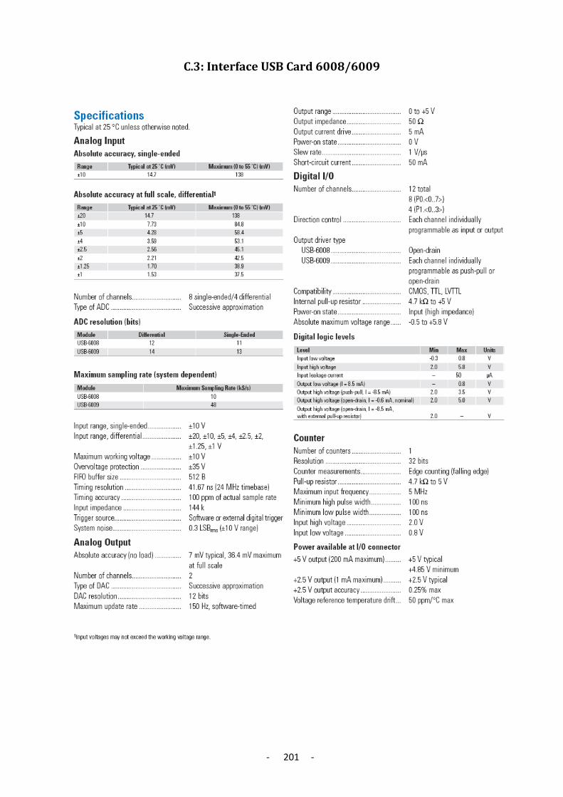
- 201 -

C.3: Interface USB Card 6008/6009

- 202 -

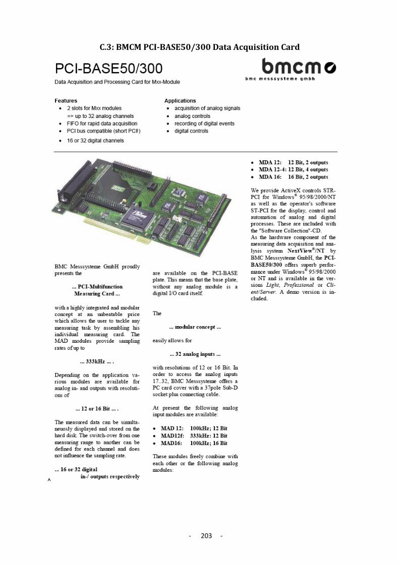
- 203 -

C.3: BMCM PCI-BASE50/300 Data Acquisition Card

^

- 204 -

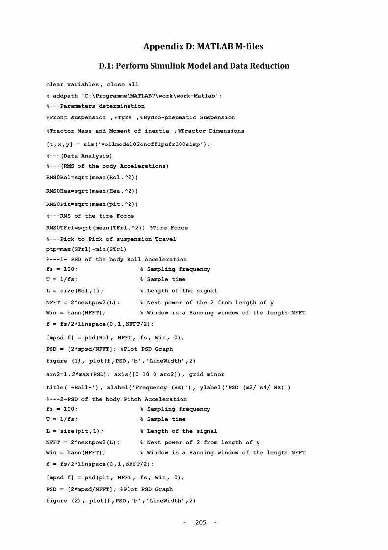
- 205 -

Appendix D: MATLAB M-files

D.1: Perform Simulink Model and Data Reduction

clear variables, close all

% addpath 'C:\Programme\MATLAB7\work\work-Matlab';

%---Parameters determination

%Front suspension ,%Tyre ,%Hydro-pneumatic Suspension

%Tractor Mass and Moment of inertia ,%Tractor Dimensions

[t,x,y] = sim('vollmodel02onoffIpufr100simp');

%---(Data Analysis)

%---(RMS of the body Accelerations)

RMS0Rol=sqrt(mean(Rol.^2))

RMS0Hea=sqrt(mean(Hea.^2))

RMS0Pit=sqrt(mean(pit.^2))

%---RMS of the tire Force

RMS0TFrl=sqrt(mean(TFrl.^2)) %Tire Force

%---Pick to Pick of suspension Travel

ptp=max(STrl)-min(STrl)

%---1- PSD of the body Roll Acceleration

fs = 100; % Sampling frequency

T = 1/fs; % Sample time

L = size(Rol,1); % Length of the signal

NFFT = 2^nextpow2(L); % Next power of the 2 from length of y

Win = hann(NFFT); % Window is a Hanning window of the length NFFT

f = fs/2*linspace(0,1,NFFT/2);

[mpsd f] = psd(Rol, NFFT, fs, Win, 0);

PSD = [2*mpsd/NFFT]; %Plot PSD Graph

figure (1), plot(f,PSD,'b','LineWidth',2)

aro2=1.2*max(PSD); axis([0 10 0 aro2]), grid minor

title('-Roll-'), xlabel('Frequency (Hz)'), ylabel('PSD (m2/ s4/ Hz)')

%---2-PSD of the body Pitch Acceleration

fs = 100; % Sampling frequency

T = 1/fs; % Sample time

L = size(pit,1); % Length of the signal

NFFT = 2^nextpow2(L); % Next power of 2 from length of y

Win = hann(NFFT); % Window is a Hanning window of the length NFFT

f = fs/2*linspace(0,1,NFFT/2);

[mpsd f] = psd(pit, NFFT, fs, Win, 0);

PSD = [2*mpsd/NFFT]; %Plot PSD Graph

figure (2), plot(f,PSD,'b','LineWidth',2)

- 206 -

aro2=1.2*max(PSD); axis([0 10 0 aro2]), grid minor

title('-Pitch-'), xlabel('Frequency (Hz)'), ylabel('PSD (m2/ s4/ Hz)')

%---3-PSD of the body Heave Acceleration

fs = 100; % Sampling frequency

T = 1/fs; % Sample time

L = size(Hea,1); % Length of the signal

NFFT = 2^nextpow2(L); % Next power of 2 from length of y

Win = hann(NFFT); % Window is a Hanning window of the length NFFT

f = fs/2*linspace(0,1,NFFT/2);

[mpsd f] = psd(Hea, NFFT, fs, Win, 0);

PSD = [2*mpsd/NFFT]; %Plot PSD Graph

figure (3), plot(f,PSD,'b','LineWidth',2)

aro2=1.2*max(PSD); axis([0 10 0 aro2]), grid minor

title('-Heave-'), xlabel('Frequency (Hz)'), ylabel('PSD (m2/ s4/ Hz)')

%---4-PSD of the wheels Acceleration

fs = 100; % Sampling frequency

T = 1/fs; % Sample time

L = size(Unrl,1); % Length of the signal

NFFT = 2^nextpow2(L); % Next power of 2 from length of y

Win = hann(NFFT); % Window is a Hanning window of the length NFFT

f = fs/2*linspace(0,1,NFFT/2);

[mpsd f] = psd(Unrl, NFFT, fs, Win, 0);

PSD = [2*mpsd/NFFT]; %Plot PSD Graph

figure (4), plot(f,PSD,'r','LineWidth',2)

aro2=1.2*max(PSD); axis([0 10 0 aro2]), grid minor

title('-Wheel rear-left-'), xlabel('Frequency (Hz)'), ylabel('PSD (m2/ s4/ Hz)')

%---5-PSD of the Dynamic Tire force

fs = 100; % Sampling frequency

T = 1/fs; % Sample time

L = size(TFrl,1); % Length of the signal

NFFT = 2^nextpow2(L); % Next power of 2 from length of y

Win = hann(NFFT); % Window is a Hanning window of the length NFFT

f = fs/2*linspace(0,1,NFFT/2);

[mpsd f] = psd(TFrl, NFFT, fs, Win, 0);

PSD = [2*mpsd/NFFT]; %Plot PSD Graph

figure (5), plot(f,PSD,'g','LineWidth',2)

aro2=1.2*max(PSD); axis([0 10 0 aro2]), grid minor

title('dynamic Tire force rl'), xlabel('Frequency (Hz)'), ylabel('PSD (N2/ Hz)')

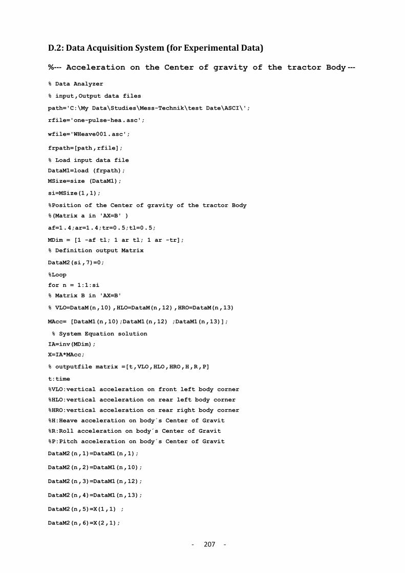
- 207 -

D.2: Data Acquisition System (for Experimental Data)

%--- Acceleration on the Center of gravity of the tractor Body ---

% Data Analyzer

% input,Output data files

path='C:\My Data\Studies\Mess-Technik\test Date\ASCI\';

rfile='one-pulse-hea.asc';

wfile='WHeave001.asc';

frpath=[path,rfile];

% Load input data file

DataM1=load (frpath);

MSize=size (DataM1);

si=MSize(1,1);

%Position of the Center of gravity of the tractor Body

%(Matrix a in 'AX=B' )

af=1.4;ar=1.4;tr=0.5;tl=0.5;

MDim = [1 -af tl; 1 ar tl; 1 ar -tr];

% Definition output Matrix

DataM2(si,7)=0;

%Loop

for n = 1:1:si

% Matrix B in 'AX=B'

% VLO=DataM(n,10),HLO=DataM(n,12),HRO=DataM(n,13)

MAcc= [DataM1(n,10);DataM1(n,12) ;DataM1(n,13)];

% System Equation solution

IA=inv(MDim);

X=IA*MAcc;

% outputfile matrix =[t,VLO,HLO,HRO,H,R,P]

t:time

%VLO:vertical acceleration on front left body corner

%HLO:vertical acceleration on rear left body corner

%HRO:vertical acceleration on rear right body corner

%H:Heave acceleration on body´s Center of Gravit

%R:Roll acceleration on body´s Center of Gravit

%P:Pitch acceleration on body´s Center of Gravit

DataM2(n,1)=DataM1(n,1);

DataM2(n,2)=DataM1(n,10);

DataM2(n,3)=DataM1(n,12);

DataM2(n,4)=DataM1(n,13);

DataM2(n,5)=X(1,1) ;

DataM2(n,6)=X(2,1);

- 208 -

DataM2(n,7)=X(3,1);

end

% Save Matrix 'DataM2' as a AscII file

fwpath=[path,wfile]

save(fwpath,'DataM2','-ASCII', '-tabs')

%------------------Tire Contact Force---------------------

%values of a querter sprung mass and an unsprung mass

spm=mt/4; unm=axm/2

%Loop

for n = 1:1:si

% Read needed parameters

%zz2fl(n): sprung mass vertical acceleration of the front left corner

%zz2fr(n): sprung mass vertical of the front right corner

%zz2rl(n): sprung mass vertical of the rear left corner

%zz2rr(n): sprung mass vertical of the rear right corner

%zz1fl(n): unsprung mass vertical acceleration of the front left corner

%zz1fr(n): unsprung mass vertical of the front right corner

%zz1rl(n): unsprung mass vertical of the rear left corner

%zz1rr(n): unsprung mass vertical of the rear right corner

zz2fl(n)=DataM(n,1), zz1fl(n)=DataM(n,5);

zz2fr(n)=DataM(n,2), zz1fr(n)=DataM(n,6);

zz2rl(n)=DataM(n,3), zz1rl(n)=DataM(n,7);

zz2rr(n)=DataM(n,4), zz1rr(n)=DataM(n,8);

%Calculation

TFfl(n)=spm*zz2fl+unm*zz1fl ; TFfr(n)=spm*zz2fr+unm*zz1fr

TFrl(n)=spm*zz2rl+unm*zz1rl; TFrr(n)=spm*zz2rr+unm*zz1rr

% outputfile matrix =[t, TFfl, TFfr, TFrl, TFrr]

t:time

% TFfl: vertical dynamic force of the front left tire

% TFfr: vertical dynamic force of the front right tire

% TFrl: vertical dynamic force of the rear left tire

% TFrr: vertical dynamic force of the rear right tire

DataM3(n,1)= DataM1(n,1);

DataM3(n,2)= TFfl(n);DataM3(n,3)= TFfr(n);

DataM3(n,4)= TFrf(n);DataM3(n,5)= TFrr(n);

end

% Save Matrix 'DataM3' as a AscII file

fwpath=[path,wfile]

save(fwpath,'DataM3','-ASCII', '-tabs')

- 209 -

Appendix E: Vehicle-Suspension Model Parameters

E.2: Tractor Body Geometry, Mass and Inertia

Table E-1 : Tires static loads of the test-tractor

Ballast Mass (kg)

lf rf lr rr Total 0 1200 1250 950 1100 4500

200 1150 1200 1100 1250 4700

Table E-2: Position of the CG of the test-tractor body relating to the axles and wheels.

Figure E-1: Top view of the test-tractor with some relevant dimensions and tires static loads

(Thiebes P. , 2006).

Figure E-2: Front and side view of the test-tractor with some relevant dimensions.

Ballast Dimension (mm)

af ar tr tl CG to font axle CG to rear axle CG to right wheel CG to left wheel

0 1289 1541 555 645 200kg 1415 1415 575 625

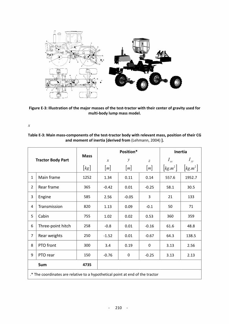
- 210 -

Figure E-3: Illustration of the major masses of the test-tractor with their center of gravity used for multi-body lump mass model.

x

Table E-3: Main mass-components of the test-tractor body with relevant mass, position of their CG and moment of inertia [derived from (Lehmann, 2004) ].

Inertia Position* Mass

yyI xxI z y x Tractor Body Part

[ ]2.mkg [ ]2.mkg [ ]m [ ]m [ ]m [ ]kg

1952.7 557.6 0.14 0.11 1.34 1252 Main frame 1

30.5 58.1 -0.25 0.01 -0.42 365 Rear frame 2

133 21 3 -0.05 2.56 585 Engine 3

71 50 -0.1 0.09 1.13 820 Transmission 4

359 360 0.53 0.02 1.02 755 Cabin 5

48.8 61.6 -0.16 0.01 -0.8 258 Three-point hitch 6

138.5 64.3 -0.67 0.01 -1.52 250 Rear weights 7

2.56 3.13 0 0.19 3.4 300 PTO front 8

2.13 3.13 -0.25 0 -0.76 150 PTO rear 9

4735 Sum

* The coordinates are relative to a hypothetical point at end of the tractor.

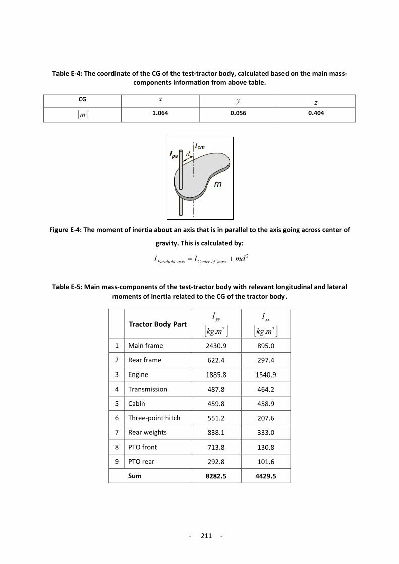
- 211 -

Table E-4: The coordinate of the CG of the test-tractor body, calculated based on the main mass-components information from above table.

CG x y z

[ ]m 1.064 0.056 0.404

Figure E-4: The moment of inertia about an axis that is in parallel to the axis going across center of

gravity. This is calculated by:

2mdII massofCenteraxisParallela +=

Table E-5: Main mass-components of the test-tractor body with relevant longitudinal and lateral moments of inertia related to the CG of the tractor body.

xxI yyI Tractor Body Part [ ]2.mkg [ ]2.mkg

895.0 2430.9 Main frame 1

297.4 622.4 Rear frame 2

1540.9 1885.8 Engine 3

464.2 487.8 Transmission 4

458.9 459.8 Cabin 5

207.6 551.2 Three-point hitch 6

333.0 838.1 Rear weights 7

130.8 713.8 PTO front 8

101.6 292.8 PTO rear 9

4429.5 8282.5 Sum

- 212 -

Table E-6: Parameters of the total mass and Inertia of the test-tractor body

Symbol Description Value Units

𝑀𝑀𝑡𝑡 Total body mass (unload) 6500 𝑘𝑘𝐾𝐾

𝐼𝐼𝑦𝑦𝑦𝑦 Moment of inertia (about pitch axis) 8282 𝐾𝐾𝐾𝐾.𝑚𝑚2

𝐼𝐼𝑥𝑥𝑥𝑥 Moment of inertia (about roll axis) 4429 𝐾𝐾𝐾𝐾.𝑚𝑚2

E.2: Tire/Axle properties

Table E-7: Tire Characteristic

Symbol Description Value Units

𝑀𝑀𝑢𝑢𝑟𝑟 Rear tire /axle mass 430 𝑘𝑘𝐾𝐾

𝑀𝑀𝑢𝑢𝑓𝑓 Front tire /axle mass 440 𝑘𝑘𝐾𝐾

𝑐𝑐𝐴𝐴𝑟𝑟 Rear tire damping coefficient 900 𝑁𝑁. 𝑁𝑁 𝑚𝑚⁄

𝑘𝑘𝐴𝐴𝑟𝑟 Rear tire stiffness 460,000 𝑁𝑁 𝑚𝑚⁄

𝑐𝑐𝐴𝐴𝑓𝑓 Front tire damping coefficient 920 𝑁𝑁. 𝑁𝑁 𝑚𝑚⁄

𝑘𝑘𝐴𝐴𝑓𝑓 Front tire stiffness 390,000 𝑁𝑁 𝑚𝑚⁄

𝐴𝐴𝑝𝑝 Tire inflation pressure 0.16 𝑀𝑀𝑃𝑃𝑟𝑟

E.3: Front Suspension Properties

Table E-8: Front Suspension Parameter

Symbol Description Value Units

𝑘𝑘𝑓𝑓 Spring stiffness 125,000 𝑁𝑁 𝑚𝑚⁄

- 213 -

E.4: Hydro-pneumatic Rear Suspension Properties

Table E-9: Parameters related to the hydro-pneumatic rear suspension of the test-tractor.

Symbol Description Value Units

𝐴𝐴𝑝𝑝 Piston area (head side) 3116 𝑚𝑚𝑚𝑚2

𝐴𝐴𝑟𝑟 Piston area (rod side) 1526 𝑚𝑚𝑚𝑚2

𝑐𝑐 Piston stroke 100 𝑚𝑚𝑚𝑚

𝑝𝑝𝑜𝑜 Pre-charge gas pressure (head side) 1.00 𝑀𝑀𝑃𝑃𝑟𝑟

𝑝𝑝𝑜𝑜 Pre-charge gas pressure (rod side) 0.50 𝑀𝑀𝑃𝑃𝑟𝑟

𝑝𝑝1 Initial pressure (head side) 4.55 𝑀𝑀𝑃𝑃𝑟𝑟

𝑝𝑝1 Initial pressure (rod side) 1.75 𝑀𝑀𝑃𝑃𝑟𝑟

𝑉𝑉𝑜𝑜 Accumulator volume (head side) 4 𝑟𝑟𝑚𝑚3 (𝐿𝐿)

𝑉𝑉𝑜𝑜 Accumulator volume (rod side) 2.5 𝑟𝑟𝑚𝑚3 (𝐿𝐿)

𝜌𝜌 Density of the oil 900 𝑘𝑘𝐾𝐾 𝑚𝑚3⁄

𝐴𝐴𝐴𝐴𝑝𝑝 Throttle cross-section (head side) 50 𝑚𝑚𝑚𝑚2

𝐴𝐴𝐴𝐴𝑟𝑟 Throttle cross-section (rod side) 38 𝑚𝑚𝑚𝑚2

𝐴𝐴𝑃𝑃𝑝𝑝 Cylinder port cross-section (head side) 55 𝑚𝑚𝑚𝑚2

𝐴𝐴𝑃𝑃𝑟𝑟 Cylinder port cross-section (rod side) 41 𝑚𝑚𝑚𝑚2

𝑡𝑡𝑝𝑝𝑟𝑟 Valve switching-on time (head side) 25 𝑚𝑚𝑁𝑁

𝑡𝑡𝑝𝑝𝑏𝑏 Valve switching-off time (head side) 35 𝑚𝑚𝑁𝑁

𝑡𝑡𝑟𝑟𝑟𝑟 Valve switching-on time (rod side) 20 𝑚𝑚𝑁𝑁

𝑡𝑡𝑟𝑟𝑏𝑏 Valve switching-off time (rod side) 30 𝑚𝑚𝑁𝑁

𝑘𝑘 Polytrophic constant 1.35 -

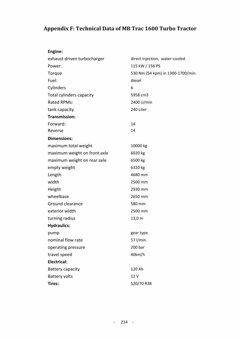
- 214 -

Appendix F: Technical Data of MB Trac 1600 Turbo Tractor

Engine:

exhaust-driven turbocharger direct injection, water-cooled

Power: 115 kW / 156 PS

Torque 530 Nm (54 kpm) in 1300-1700/min.

Fuel: diesel

Cylinders 6

Total cylinders capacity 5958 cm3

Rated RPMs: 2400 U/min

tank capacity 240 Liter

Transmission:

Forward: 14

Reverse 14

Dimensions:

maximum total weight 10000 kg

maximum weight on front axle 6020 kg

maximum weight on rear axle 6500 kg

empty weight 6320 kg

Length 4680 mm

width 2500 mm

Height 2930 mm

wheelbase 2650 mm

Ground clearance 580 mm

exterior width 2500 mm

turning radius 13,0 m

Hydraulics:

pump gear type

nominal flow rate 57 l/min.

operating pressure 200 bar

travel speed 40km/h

Electrical:

Battery capacity 120 Ah

Battery volts 12 V

Tires: 520/70 R38