sat modulo monotonic theories - cs.ubc.ca · sat modulo monotonic theories by sam bayless b. sc.,...
TRANSCRIPT
SAT Modulo Monotonic Theories
by
Sam Bayless
B. Sc., The University of British Columbia, 2010
A THESIS SUBMITTED IN PARTIAL FULFILLMENT
OF THE REQUIREMENTS FOR THE DEGREE OF
Doctor of Philosophy
in
THE FACULTY OF GRADUATE AND POSTDOCTORAL STUDIES
(Computer Science)
The University of British Columbia
(Vancouver)
March 2017
c© Sam Bayless, 2017
Abstract
Satisfiability Modulo Theories (SMT) solvers are a class of efficient constraint
solvers which form integral parts of many algorithms. Over the years, dozens of
different Satisfiability Modulo Theories solvers have been developed, supporting
dozens of different logics. However, there are still many important applications for
which specialized SMT solvers have not yet been developed.
We develop a framework for easily building efficient SMT solvers for previ-
ously unsupported logics. Our techniques apply to a wide class of logics which we
call monotonic theories, which include many important elements of graph theory
and automata theory.
Using this SAT Modulo Monotonic Theories framework, we created a new SMT
solver, MONOSAT. We demonstrate that MONOSAT improves the state of the art
across a wide body of applications, ranging from circuit layout and data center
management to protocol synthesis — and even to video game design.
ii
Preface
The work in this thesis was developed in a collaboration between the Integrated
Systems Design Laboratory (ISD) and the Bioinformatics and Empirical & Theo-
retical Algorithmics Laboratory (BETA), at the University of British Columbia.
This thesis includes elements of several published and unpublished works. In
addition to my own contributions, each of these works includes significant contri-
butions from my co-authors, as detailed below.
Significant parts of the material found in chapters 3, 4, 5, 7, and 6.1 appeared
previously at the conference of the Association for the Advancement of Artificial
Intelligence, 2015, with co-authors N. Bayless, H. H. Hoos, and A. J. Hu. I was the
lead investigator in this work, responsible for the initial concept and its execution,
for conducting all experiments, and for writing the manuscript.
Significant parts of the material found in Chapter 8 appeared previously at the
International Conference on Computer Aided Verification, 2016, with co-authors
T. Klenze and A. J. Hu. In this work, Tobias Klenze was the lead investigator; I
also made significant contributions throughout, including playing a supporting role
in the implementation. I was also responsible for conducting all experiments.
Significant parts of Section 6.2 were previously published at the International
Conference on ComputerAided Design, 2016, with co-authors H. H. Hoos, and
A. J. Hu. In this work, I was the lead investigator, responsible for conducting all
experiments, and for writing the manuscript. This work also included assistance
and insights from Jacob Bayless.
Finally, Section 6.3 is based on unpublished work in collaboration with co-
authors N. Kodirov, I. Beschastnikh, H. H. Hoos, and A. J. Hu, in which I was the
lead investigator, along with Nodir Kodirov. In this work, I was responsible for the
implementation, as well as conducting all experiments and writing the manuscript.
iii
Table of Contents
Abstract . . . . . . . . . . . . . . . . . . . . . . . . . . . . . . . . . . . . ii
Preface . . . . . . . . . . . . . . . . . . . . . . . . . . . . . . . . . . . . iii
Table of Contents . . . . . . . . . . . . . . . . . . . . . . . . . . . . . . iv
List of Tables . . . . . . . . . . . . . . . . . . . . . . . . . . . . . . . . . viii
List of Figures . . . . . . . . . . . . . . . . . . . . . . . . . . . . . . . . ix
Acknowledgments . . . . . . . . . . . . . . . . . . . . . . . . . . . . . . xi
1 Introduction . . . . . . . . . . . . . . . . . . . . . . . . . . . . . . . 1
2 Background . . . . . . . . . . . . . . . . . . . . . . . . . . . . . . . 32.1 Boolean Satisfiability . . . . . . . . . . . . . . . . . . . . . . . . 3
2.2 Boolean Satisfiability Solvers . . . . . . . . . . . . . . . . . . . . 6
2.2.1 DPLL SAT Solvers . . . . . . . . . . . . . . . . . . . . . 7
2.2.2 CDCL SAT Solvers . . . . . . . . . . . . . . . . . . . . . 9
2.3 Many-Sorted First Order Logic & Satisfiability Modulo Theories . 13
2.4 Satisfiability Modulo Theories Solvers . . . . . . . . . . . . . . 17
2.5 Related Work . . . . . . . . . . . . . . . . . . . . . . . . . . . . 22
3 SAT Modulo Monotonic Theories . . . . . . . . . . . . . . . . . . . 243.1 Monotonic Predicates . . . . . . . . . . . . . . . . . . . . . . . 24
3.2 Monotonic Theories . . . . . . . . . . . . . . . . . . . . . . . . . 28
iv
4 A Framework for SAT Modulo Monotonic Theories . . . . . . . . . 304.1 Theory Propagation for Finite Monotonic Theories . . . . . . . . 32
4.2 Conflict Analysis for Finite Monotonic Theories . . . . . . . . . . 40
4.3 Compositions of Monotonic Functions . . . . . . . . . . . . . . . 43
4.4 Monotonic Theories of Partially Ordered Sorts . . . . . . . . . . . 48
4.5 Theory Combination and Infinite Domains . . . . . . . . . . . . . 52
5 Monotonic Theory of Graphs . . . . . . . . . . . . . . . . . . . . . . 555.1 A Monotonic Graph Solver . . . . . . . . . . . . . . . . . . . . . 56
5.2 Monotonic Graph Predicates . . . . . . . . . . . . . . . . . . . . 59
5.2.1 Graph Reachability . . . . . . . . . . . . . . . . . . . . . 60
5.2.2 Acyclicity . . . . . . . . . . . . . . . . . . . . . . . . . . 65
5.3 Weighted Graphs & Bitvectors . . . . . . . . . . . . . . . . . . . 68
5.3.1 Maximum Flow . . . . . . . . . . . . . . . . . . . . . . . 68
5.4 Conclusion . . . . . . . . . . . . . . . . . . . . . . . . . . . . . 74
6 Graph Theory Applications . . . . . . . . . . . . . . . . . . . . . . . 766.1 Procedural Content Generation . . . . . . . . . . . . . . . . . . . 76
6.2 Escape Routing . . . . . . . . . . . . . . . . . . . . . . . . . . . 85
6.2.1 Multi-Layer Escape Routing in MONOSAT . . . . . . . . 87
6.2.2 Evaluation . . . . . . . . . . . . . . . . . . . . . . . . . 90
6.3 Virtual Data Center Allocation . . . . . . . . . . . . . . . . . . . 94
6.3.1 Problem Formulation . . . . . . . . . . . . . . . . . . . . 94
6.3.2 Multi-Commodity Flow in MONOSAT . . . . . . . . . . 96
6.3.3 Encoding Multi-Path VDC Allocation . . . . . . . . . . . 98
6.3.4 Evaluation . . . . . . . . . . . . . . . . . . . . . . . . . 99
6.4 Conclusion . . . . . . . . . . . . . . . . . . . . . . . . . . . . . 107
7 Monotonic Theory of Geometry . . . . . . . . . . . . . . . . . . . . 1087.1 Geometric Predicates of Convex Hulls . . . . . . . . . . . . . . . 111
7.1.1 Areas of Convex Hulls . . . . . . . . . . . . . . . . . . . 111
7.1.2 Point Containment for Convex Hulls . . . . . . . . . . . . 112
7.1.3 Line-Segment Intersection for Convex Hulls . . . . . . . . 115
7.1.4 Intersection of Convex Hulls . . . . . . . . . . . . . . . . 116
v
7.2 Applications . . . . . . . . . . . . . . . . . . . . . . . . . . . . . 118
8 Monotonic Theory of CTL . . . . . . . . . . . . . . . . . . . . . . . 1228.1 Background . . . . . . . . . . . . . . . . . . . . . . . . . . . . . 124
8.2 CTL Operators as Monotonic Functions . . . . . . . . . . . . . . 127
8.3 Theory Propagation for CTL Model Checking . . . . . . . . . . . 130
8.4 Conflict Analysis for the Theory of CTL . . . . . . . . . . . . . . 134
8.5 Implementation and Optimizations . . . . . . . . . . . . . . . . . 136
8.5.1 Symmetry Breaking . . . . . . . . . . . . . . . . . . . . 136
8.5.2 Preprocessing . . . . . . . . . . . . . . . . . . . . . . . . 137
8.5.3 Wildcard Encoding for Concurrent Programs . . . . . . . 137
8.6 Experimental Results . . . . . . . . . . . . . . . . . . . . . . . . 139
8.6.1 The Original Clarke-Emerson Mutex . . . . . . . . . . . 140
8.6.2 Mutex with Additional Properties . . . . . . . . . . . . . 141
8.6.3 Readers-Writers . . . . . . . . . . . . . . . . . . . . . . 143
9 Conclusions and Future Work . . . . . . . . . . . . . . . . . . . . . 146
Bibliography . . . . . . . . . . . . . . . . . . . . . . . . . . . . . . . . . 148
A The MONOSAT Solver . . . . . . . . . . . . . . . . . . . . . . . . . 169
B Monotonic Theory of Bitvectors . . . . . . . . . . . . . . . . . . . . 173
C Supporting Materials . . . . . . . . . . . . . . . . . . . . . . . . . . 179C.1 Proof of Lemma 4.1.1 . . . . . . . . . . . . . . . . . . . . . . . . 179
C.2 Proof of Correctness for Algorithm 7 . . . . . . . . . . . . . . . . 181
C.3 Encoding of Art Gallery Synthesis . . . . . . . . . . . . . . . . . 184
D Monotonic Predicates . . . . . . . . . . . . . . . . . . . . . . . . . . 187D.1 Graph Predicates . . . . . . . . . . . . . . . . . . . . . . . . . . 187
D.1.1 Reachability . . . . . . . . . . . . . . . . . . . . . . . . 187
D.1.2 Acyclicity . . . . . . . . . . . . . . . . . . . . . . . . . . 188
D.1.3 Connected Components . . . . . . . . . . . . . . . . . . 189
D.1.4 Shortest Path . . . . . . . . . . . . . . . . . . . . . . . . 190
vi
D.1.5 Maximum Flow . . . . . . . . . . . . . . . . . . . . . . . 190
D.1.6 Minimum Spanning Tree Weight . . . . . . . . . . . . . . 192
D.2 Geometric Predicates . . . . . . . . . . . . . . . . . . . . . . . . 193
D.2.1 Area of Convex Hulls . . . . . . . . . . . . . . . . . . . . 193
D.2.2 Point Containment for Convex Hulls . . . . . . . . . . . . 194
D.2.3 Line-Segment Intersection for Convex Hulls . . . . . . . . 195
D.2.4 Intersection of Convex Hulls . . . . . . . . . . . . . . . . 196
D.3 Pseudo-Boolean Constraints . . . . . . . . . . . . . . . . . . . . 197
D.4 CTL Model Checking . . . . . . . . . . . . . . . . . . . . . . . . 198
vii
List of Tables
Table 6.1 Reachability constraints in terrain generation. . . . . . . . . . 79
Table 6.2 Runtime results for shortest paths constraints in Diorama. . . . 80
Table 6.3 Runtime results for connected components constraints in Dio-
rama. . . . . . . . . . . . . . . . . . . . . . . . . . . . . . . . 81
Table 6.4 Runtime results for maximum flow constraints in Diorama. . . 82
Table 6.5 Maze generation using minimum spanning tree constraints. . . 84
Table 6.6 Multi-layer escape routing with blind vias. . . . . . . . . . . . 92
Table 6.7 Multi-layer escape routing with through-vias. . . . . . . . . . . 93
Table 6.8 Data centers with tree topologies. . . . . . . . . . . . . . . . . 101
Table 6.9 Data centers with FatTree and BCube Topologies. . . . . . . . 103
Table 6.10 Hadoop VDCs allocated on data centers. . . . . . . . . . . . . 106
Table 7.1 Art gallery synthesis results. . . . . . . . . . . . . . . . . . . 120
Table 8.1 Results on the mutual exclusion example. . . . . . . . . . . . . 140
Table 8.2 Results on the mutual exclusion with additional properties . . . 142
Table 8.3 Results on the readers-writers instances. . . . . . . . . . . . . 144
viii
List of Figures
Figure 2.1 Example of Tseitin transformation . . . . . . . . . . . . . . . 5
Figure 2.2 A first order formula and associated Boolean skeleton. . . . . 18
Figure 3.1 A finite symbolic graph. . . . . . . . . . . . . . . . . . . . . 27
Figure 5.1 A finite symbolic graph and satisfying assignment. . . . . . . 56
Figure 5.2 A finite symbolic graph, under assignment. . . . . . . . . . . 60
Figure 5.3 Summary of our theory solver implementation of reachability. 61
Figure 5.4 Results on reachability constraints. . . . . . . . . . . . . . . . 64
Figure 5.5 Summary of our theory solver implementation of acyclicity. . 65
Figure 5.6 Results on acyclicity constraints. . . . . . . . . . . . . . . . . 67
Figure 5.7 Maximum flow predicate example. . . . . . . . . . . . . . . . 69
Figure 5.8 Summary of our theory solver implementation of maximum flow. 71
Figure 5.9 Results on maximum flow constraints. . . . . . . . . . . . . . 73
Figure 6.1 Generated terrain . . . . . . . . . . . . . . . . . . . . . . . . 78
Figure 6.2 Random Mazes . . . . . . . . . . . . . . . . . . . . . . . . . 83
Figure 6.3 An example multi-layer escape routing. . . . . . . . . . . . . 85
Figure 6.4 Multi-layer escape routing with simultaneous via-placement. . 87
Figure 6.5 Symbolic nodes and edges. . . . . . . . . . . . . . . . . . . . 88
Figure 6.6 Constraints enforcing different via models. . . . . . . . . . . 90
Figure 7.1 Convex hull of a symbolic point set. . . . . . . . . . . . . . . 109
Figure 7.2 Under- and over-approximative convex hulls. . . . . . . . . . 109
Figure 7.3 Point containment for convex hulls . . . . . . . . . . . . . . . 113
ix
Figure 7.4 Line-segment intersection for convex hulls . . . . . . . . . . 114
Figure 7.5 Intersection of convex hulls . . . . . . . . . . . . . . . . . . 116
Figure 7.6 A separating axis between two convex hulls. . . . . . . . . . . 118
Figure 7.7 Art gallery synthesis. . . . . . . . . . . . . . . . . . . . . . . 120
Figure 8.1 An example CTL formula and Kripke structure. . . . . . . . . 123
x

Acknowledgments
Alan and Holger, for giving me both the freedom and the support that I needed. The
students I have collaborated with, including Celina, Mike, Nodir, Tobias, Kuba,
and many others who have passed through our lab, for being a continuing source
of inspiration. My parents and siblings, for everything else.
And the many shelves worth of science fiction that got me through it all....
xi
Chapter 1
Introduction
Constraint solvers have widespread applications in all areas of computer science,
and can be found in products ranging from drafting tools [18] to user interfaces [20].
Intuitively, constraint solvers search for a solution to a logical formula, with differ-
ent constraint solvers using different reasoning methods and supporting different
logics.
One particular family of constraint solvers, Boolean satisfiability (SAT) solvers,
has made huge strides in the last two decades. Fast SAT solvers now form the core
engines of many other important algorithms, with applications to AI planning (e.g.,
[138, 174]), hardware verification (e.g., [35, 40, 148]), software verification (e.g.,
[50, 57]), and even to program synthesis (e.g., [136, 184]).
Building on this success, the introduction of a plethora of Satisfiability Modulo
Theories (SMT) solvers (see, e.g., [44, 70, 81, 192]) has allowed SAT solvers to
efficiently solve problems from many new domains, most notably from arithmetic
(e.g., [80, 100, 190]) and data structures (e.g., [29, 173, 191]). In fact, since their
gradual formalization in the 1990’s and 2000’s, SMT solvers — and, in particular,
lazy SMT solvers, which delay encoding the formula into Boolean logic — have
been introduced for dozens of logics, greatly expanding the scope of problems that
SAT solvers can effectively tackle in practice.
Unfortunately, many important problem domains, including elements of graph
and automata theory, do not yet have dedicated SMT solvers. In Chapter 2, we
review the literature on SAT and SMT solvers, and the challenges involved in de-
1

Chapter 1. Introduction
signing SMT solvers for previously unsupported theories.
We have identified a class of theories for which one can create efficient SMT
solvers with relative ease. These theories, which we term monotonic theories, are
integral to many problem domains with major real-world applications in computer
networks, computer-aided design, and protocol synthesis. In Chapter 3, we for-
mally define what constitutes a monotonic theory, and in Chapter 4 we describe
the SAT Modulo Monotonic Theories (SMMT) framework, a comprehensive set of
techniques for building efficient lazy SMT solvers for monotonic theories. (Further
practical implementation details can be found in Appendix A.)
As we will show, important properties from graph theory (Chapters 5, 6), ge-
ometry (Chapter 7), and automata theory (Chapter 8), among many others, can
be modeled as monotonic theories and solved efficiently in practice. Using the
SMMT framework, we have implemented a lazy SMT solver (MONOSAT) sup-
porting these theories, with greatly improved performance over a range of impor-
tant applications, from circuit layout and data center management to protocol syn-
thesis — and even to video game design.
We do not claim that solvers built using our techniques are always the best
approach to solving monotonic theories — to the contrary, we can demonstrate at
least some cases where there exist dedicated solvers for monotonic theories that
out-perform our generic approach.1 However, this thesis does make three central
claims:
1. A wide range of important, useful monotonic theories exist.
2. Many of these theories can be better solved using the constraint solver de-
scribed in this thesis than by any previous constraint solver.
3. The SAT Modulo Monotonic Theories framework described in this thesis
can be used to build efficient constraint solvers.
1Specifically, in Chapter 5 we discuss some applications in which our graph theory solver is out-performed by other solvers. More generally, many arithmetic theories can be modeled as monotonictheories, for which there already exist highly effective SMT solvers against which our approach isnot competitive. Examples include linear arithmetic, difference logic, and, as we will discuss later,pseudo-Boolean constraints.
2

Chapter 2
Background
Before introducing the SAT Modulo Monotonic Theories (SMMT) framework in
Chapters 3 and 4, we review several areas of relevant background. First, we re-
view the theoretical background of Boolean satisfiability, and then survey the most
relevant elements of modern conflict-driven clause-learning (CDCL) SAT solvers.
Then we review the aspects of many-sorted first-order logic that form the theoreti-
cal background of Satisfiability Modulo Theories (SMT) solvers, and describe the
basic components of lazy SMT solvers.
2.1 Boolean SatisfiabilityBoolean satisfiability (SAT) is the problem of determining, for a given proposi-
tional formula, whether or not there exists a truth assignment to the Boolean vari-
ables of that formula such that the formula evaluates to TRUE (we will define this
more precisely shortly). SAT is a fundamental decision problem in computer sci-
ence, and the first to be proven NP-Complete [61]. In addition to its important
theoretical properties, many real-world problems can be efficiently modeled as
SAT problems, making solving Boolean satisfiability in practice an important prob-
lem to tackle. Surprisingly, following a long period of stagnation in SAT solvers
(from the 1960s to the early 1990s), great strides on several different fronts have
now been made in solving SAT problems efficiently, allowing for wide classes of
instances to be solved quickly enough to be useful in practice. Major advance-
3
Chapter 2. Background
ments in SAT solver technology include the introduction of WALKSAT [180] and
other stochastic local search solvers in the early 1990s, and the development of
GRASP [146], CHAFF [151] and subsequent CDCL solvers in the late 1990’s and
following decade. We will review these in Section 2.2.
A Boolean propositional formula is a formula over Boolean variables that, for
any given assignment to those variables, evaluates to either TRUE or FALSE. For-
mally, a propositional formula φ can be a literal, which is either a Boolean vari-
able v or its negation ¬v; or it may be built from other propositional formulas
using, e.g. one of the standard binary logical operators ¬φ0,(φ0 ∧ φ1), (φ0 ∨ φ1),
(φ0 =⇒ φ1), . . ., with φi a Boolean formula. A truth assignmentM : v 7→ T,Ffor φ is a map from the Boolean variables of φ to TRUE,FALSE. It is also often
convenient to treat a truth assignment as a set of literals, containing the literal v iff
v 7→ T ∈M, and the literal ¬v iff v 7→ F ∈M. A truth assignmentM is a complete
truth assignment for a formula φ if it maps all variables in the formula to assign-
ments; otherwise it is a partial truth assignment. A formula φ is satisfiable if there
exists one or more complete truth assignments to the Boolean variables of φ such
that the formula evaluates to TRUE; otherwise it is unsatisfiable. A propositional
formula is valid or tautological if it evaluates to TRUE under all possible complete
assignments;1 a propositional formula is invalid if it evaluates to FALSE under at
least one assignment.
A complete truth assignment M that satisfies the formula φ may be called a
model of φ , written M |= φ (especially in the context of first order logic); or it
may be called a witness for the satisfiability of φ (in the context of SAT as anNP-
complete problem). A partial truth assignment M is an implicant of φ , written
M =⇒ φ , if all possible completions of the partial assignmentM into a complete
assignment must satisfy φ ; a partial assignment M is a prime implicant of φ if
M =⇒ φ and no proper subset ofM is itself an implicant of φ .2
In most treatments, Boolean satisfiability is assumed to be applied only to
propositional formulas in Conjunctive Normal Form (CNF), a restricted subset of
1In purely propositional logic, there is no distinction between valid formulas and tautologies;however, in most presentations of first order logic there is a distinction between the two concepts.
2There is also a notion of minimal models, typically defined as complete, satisfying truth assign-ments of φ in which a (locally) minimal number of variables are assigned TRUE.
4
Chapter 2. Background
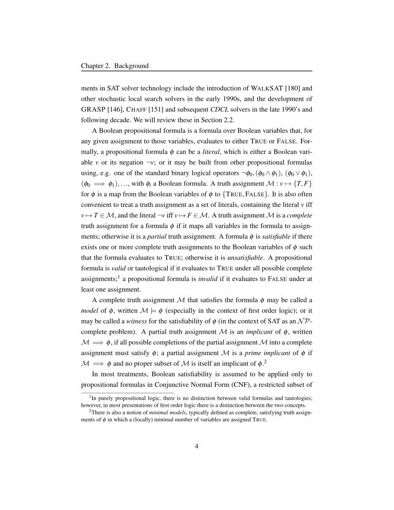
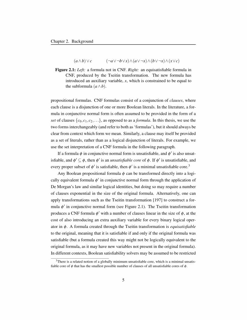
(a∧b)∨ c (¬a∨¬b∨x)∧(a∨¬x)∧(b∨¬x)∧(x∨c)
Figure 2.1: Left: a formula not in CNF. Right: an equisatisfiable formula inCNF, produced by the Tseitin transformation. The new formula hasintroduced an auxiliary variable, x, which is constrained to be equal tothe subformula (a∧b).
propositional formulas. CNF formulas consist of a conjunction of clauses, where
each clause is a disjunction of one or more Boolean literals. In the literature, a for-
mula in conjunctive normal form is often assumed to be provided in the form of a
set of clauses c0,c1,c2, . . ., as opposed to as a formula. In this thesis, we use the
two forms interchangeably (and refer to both as ‘formulas’), but it should always be
clear from context which form we mean. Similarly, a clause may itself be provided
as a set of literals, rather than as a logical disjunction of literals. For example, we
use the set interpretation of a CNF formula in the following paragraph.
If a formula φ in conjunctive normal form is unsatisfiable, and φ ′ is also unsat-
isfiable, and φ ′ ⊆ φ , then φ ′ is an unsatisfiable core of φ . If φ ′ is unsatisfiable, and
every proper subset of φ ′ is satisfiable, then φ ′ is a minimal unsatisfiable core.3
Any Boolean propositional formula φ can be transformed directly into a logi-
cally equivalent formula φ ′ in conjunctive normal form through the application of
De Morgan’s law and similar logical identities, but doing so may require a number
of clauses exponential in the size of the original formula. Alternatively, one can
apply transformations such as the Tseitin transformation [197] to construct a for-
mula φ ′ in conjunctive normal form (see Figure 2.1). The Tseitin transformation
produces a CNF formula φ ′ with a number of clauses linear in the size of φ , at the
cost of also introducing an extra auxiliary variable for every binary logical oper-
ator in φ . A formula created through the Tseitin transformation is equisatisfiable
to the original, meaning that it is satisfiable if and only if the original formula was
satisfiable (but a formula created this way might not be logically equivalent to the
original formula, as it may have new variables not present in the original formula).
In different contexts, Boolean satisfiability solvers may be assumed to be restricted
3There is a related notion of a globally minimum unsatisfiable core, which is a minimal unsatis-fiable core of φ that has the smallest possible number of clauses of all unsatisfiable cores of φ .
5
Chapter 2. Background
to operating on CNF formulas, or they may be allowed to take non-normal-form
inputs. As the Tseitin transformation (and similar transformations, such as the
Plaisted-Greenbaum [167] transformation) can be applied in linear time, in many
contexts it is simply left unspecified whether a Boolean satisfiability solver is re-
stricted to CNF or not, with the assumption that a non-normal form formula can be
implicitly transformed into CNF if required.4
Boolean satisfiability is an NP-complete problem, and all known algorithms
for solving it require at least exponential time in the worst case. Despite this, as
we will discuss in the next section, SAT solvers often can solve even very large
instances with millions of clauses and variables quite easily in practice.
2.2 Boolean Satisfiability SolversSAT solvers have a long history of development, but at present, successful solvers
can be roughly divided into complete solvers (which can both find a satisfying
solution to a given formula, if such a solution exists, or prove that no such solution
exists) and incomplete solvers, which are able to find satisfying solutions if they
exist, but cannot prove that a formula is unsatisfiable.
Incomplete solvers are primarily stochastic local search (SLS) solvers, which
are only guaranteed to terminate on satisfiable instances, originally introduced in
the WALKSAT [180] solver. Most complete SAT solvers can trace their develop-
ment back to the resolution rule([66]), and the Davis-Putnam-Logemann-Loveland
(DPLL) algorithm [67]. At the present time, DPLL-based complete solvers have
diverged into two main branches: look-ahead solvers (e.g., [97]), which perform
well on unsatisfiable ‘random’ (phase transition) instances (e.g., [76]), or on diffi-
cult ‘crafted’ instances (e.g., [118]); and Conflict-Driven Clause-Learning (CDCL)
solvers, which have their roots in the GRASP [146] and CHAFF [151] solvers
(along with many other contributing improvements over the years), which perform
well on so-called application, or industrial, instances. These divisions have solidi-
fied in the last 15 years: in all recent SAT competitions [134], CDCL solvers have
won in the applications/industrial category, look-ahead solvers have won in the
4There are also some SAT solvers specifically designed to work on non-normal-form inputs(e.g., [163, 204]), with applications to combinatorial equivalence checking.
6
Chapter 2. Background
crafted and unsatisfiable/mixed random categories, while stochastic local search
solvers have won in the satisfiable random instances category.
In this thesis, we are primarily interested in CDCL solvers, and their rela-
tion to SMT solvers. Other branches of development exist (such as Stalmarck’s
method [188], and Binary Decision Diagrams [45]), but although BDDs in particu-
lar are competitive with SAT solvers in some applications (such as certain problems
arising in formal verification [168]), neither of these techniques has been success-
ful in any recent SAT competitions. There have been solvers which combine some
of the above mentioned SAT solver strategies, such as Cube and Conquer [119],
which combines elements of CDCL and lookahead solvers, or SATHYS, which
combines techniques from SLS and CDCL solvers [17], with mixed success. As
CDCL solvers developed out of the DPLL algorithm, we will briefly review DPLL
before moving on to CDCL.
2.2.1 DPLL SAT Solvers
The Davis-Putnam-Logemann-Loveland (DPLL) algorithm is shown in Algorithm
1. DPLL combines recursive case-splitting (over the space of truth assignments to
the variables in the CNF formula) with a particularly effective search-space pruning
strategy and deduction technique, unit propagation.5
DPLL takes as input a propositional formula φ in conjunctive normal form,
and repeatedly applies the unit propagation rule (and optionally the pure-literal
elimination rule) until a fixed point is reached. After applying unit propagation, if
all clauses have been satisfied (and removed from φ ), DPLL returns TRUE. If any
clause has been violated (represented as an empty clause), DPLL returns FALSE.
Otherwise, DPLL picks an unassigned Boolean variable v from φ , assigning v to
either TRUE or FALSE, and recursively applies DPLL to both cases. These free
assignments are called decisions.
The unit propagation rule takes a formula φ in conjunctive normal form, and
checks if there exists a clause in φ that contains only a single literal l (a unit clause).
Unit propagation then removes any clauses in φ containing l, and removes from
each remaining clause any occurrence of ¬l. After this process, φ does not contain
5Unit propagation is also referred to as Boolean Constraint Propagation; in the constraint pro-gramming literature, it would be considered an example of the arc consistency rule [199].
7
Chapter 2. Background
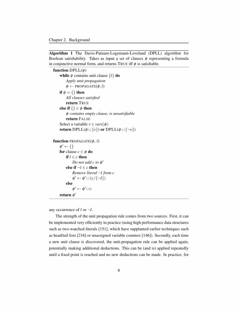
Algorithm 1 The Davis-Putnam-Logemann-Loveland (DPLL) algorithm forBoolean satisfiability. Takes as input a set of clauses φ representing a formulain conjunctive normal form, and returns TRUE iff φ is satisfiable.
function DPLL(φ )while φ contains unit clause l do
Apply unit propagationφ ← PROPAGATE(φ , l)
if φ = thenAll clauses satisfiedreturn TRUE
else if ∈ φ thenφ contains empty clause, is unsatisfiablereturn FALSE
Select a variable v ∈ vars(φ)return DPLL(φ ∪v) or DPLL(φ ∪¬v)
function PROPAGATE(φ , l)φ ′←for clause c ∈ φ do
if l ∈ c thenDo not add c to φ ′
else if ¬l ∈ c thenRemove literal ¬l from cφ ′← φ ′∪ (c/¬l)
elseφ ′← φ ′∪ c
return φ ′
any occurrence of l or ¬l.
The strength of the unit propagation rule comes from two sources. First, it can
be implemented very efficiently in practice (using high performance data structures
such as two-watched-literals [151], which have supplanted earlier techniques such
as head/tail lists [216] or unassigned variable counters [146]). Secondly, each time
a new unit clause is discovered, the unit-propagation rule can be applied again,
potentially making additional deductions. This can be (and is) applied repeatedly
until a fixed point is reached and no new deductions can be made. In practice, for
8
Chapter 2. Background
many common instances, the unit propagation rule ends up very cheaply making
long chains of deductions, allowing it to eliminate large parts of the search space.
Because it makes many deductions, and because it does so inexpensively, the unit
propagation rule is very hard to augment without unduly slowing down the solver.
Other deduction rules have been proposed; in particular, the original DPLL algo-
rithm also applied pure literal elimination (in which any variable occurring in only
one polarity throughout the CNF is assigned that polarity), however, modern SAT
solvers almost always apply the unit propagation rule exclusively.6
In practice, the decision of which variable to pick, and whether to test the posi-
tive assignment (v) or the negative assignment (¬v), has an enormous impact on the
performance of the algorithm, and so careful implementations will put significant
effort into good decision heuristics. Although many heuristics have been proposed,
most current solvers use the VSIDS heuristic (introduced in Chaff), with a minor-
ity using the Berkmin [109] heuristic. Both of these heuristics choose which vari-
able to split on next, but do not select which polarity to try first; common polarity
selection heuristics include Jeroslow-Wang [135], phase-learning [166], choosing
randomly, or simply always choosing one of TRUE or FALSE first.
2.2.2 CDCL SAT Solvers
Conflict-Driven Clause Learning (CDCL) SAT solvers consist of a number of ex-
tensions and improvements to DPLL. In addition to the improved decision heuris-
tics and unit-propagation data structures discussed in the previous section, a few of
the key improvements include:
1. Clause learning
2. Non-chronological backtracking
3. Learned-clause discarding heuristics
4. Pre-processing
5. Restarts6Note that this generalization applies mostly to CDCL SAT solvers. In contrast, solvers that
extend the CDCL framework to other logics, and in particular SMT solvers, sometimes do applyadditional deduction rules.
9

Chapter 2. Background
Algorithm 2 A simplified Conflict-Driven Clause-Learning (CDCL) solver. Takesas input a set of clauses φ representing a formula in conjunctive normal form, andreturns TRUE iff φ is satisfiable. PROPAGATE applies unit propagation to a partialassignment, adding any unit literals to the assignment, and potentially finding aconflict clause. ANALYZE and BACKTRACK perform clause learning and non-chronological backtracking, as described in the text. SIMPLIFY uses heuristics toidentify and discard some of the learned clauses. Lines marked occasionally areonly applied when heuristic conditions are met.
function SOLVE(φ )level← 0assign←loop
if PROPAGATE(assign) returns a conflict thenif level = 0 then
return FALSE
c,backtrackLevel← ANALYZE(conflict)φ ← φ ∪ clevel← BACKTRACK(backtrackLevel,assign)
elseif All variables are assigned then
return TRUE
if level > 0 then occasionally restart the solver to level 0level← BACKTRACK(0,assign)
if level = 0 thenOccasionally discard some learned or redundant clausesφ ← SIMPLIFY(φ)
Select unassigned literal llevel← level +1assign[l]← TRUE
Of these, the first two are the most relevant to this thesis, so we will restrict our
attention to those. Clause learning and non-chronological backtracking (sometimes
‘back-jumping’) were originally developed independently, but in current solvers
they are tightly integrated techniques. In Algorithm 2, we describe a simplified
CDCL loop. Unlike our recursive presentation of DPLL, this presentation is in a
stateful, iterative form, in which PROPAGATE operates on an assignment structure,
rather than removing literals and clauses from φ .
10
Chapter 2. Background
Clause learning, introduced in the SAT solver GRASP [146], is a form of ‘no-
good’ learning [74], a common technique in CSP solvers for pruning unsatisfiable
parts of the search space. When a conflict occurs in a DPLL solver (that is, when
φ contains an empty clause), the solver simply backtracks past the most recent
decision and then continues exploring the search tree. In contrast, when a clause-
learning SAT solver encounters a conflict, it derives a learned clause, c, not present
in φ , that serves to ‘explain’ (in a precise sense) the conflict. This learned clause
is then appended to φ . Specifically, the learned clause is such that if the clause
had been present in the formula, unit propagation would have prevented (at least)
one of the decisions made by the solver that resulted in the conflict. By adding
this new clause to φ , the solver is prevented in the future from making the same
set of decisions that led to the current conflict. In this sense, learned clauses can
be seen as augmenting or strengthening the unit propagation rule. Learned clauses
are sometimes called redundant clauses, because they can be added to or removed
from the formula without removing any solutions from the formula.
After a conflict, there may be many choices for the learned clause. Modern
CDCL solvers learn asserting clauses, which have two additional properties: 1) all
literals in the clause are false in the current assignment, and 2) exactly one literal
in the clause was assigned at the current decision level. Although many possible
strategies for learning clauses have been proposed (see, e.g., [32, 146]), by far
the dominant strategy is the first unique implication point (1-UIP) method [218],
sometimes augmented with post-processing to further reduce the size of the clause
([84, 186]).
Each time a conflict occurs, the solver learns a new clause, eliminating at least
one search path (the one that led to the conflict). In practice, clauses are often
much smaller than the number of decisions made by the solver, and hence each
clause may eliminate many search paths, including ones that have not yet been
explored by the solver. Eventually, this process will either force the solver to find
a satisfying assignment, or the solver will encounter a conflict in which no new
clause can be learned (because no decisions have yet been made by the solver).
In this second case, the formula is unsatisfiable, and the solver will terminate. A
side benefit of clause learning is that as the clauses serve to implicitly prevent the
solver from exploring previously searched paths, the solver is freed to explore paths
11
Chapter 2. Background
in any order without having to explicitly keep track of previously explored paths.
This allows CDCL solvers to apply restarts cheaply, without losing the progress
they have already made.
In a DPLL solver, when a conflict is encountered, the solver backtracks up
the search tree until it reaches the most recent decision where only one branch
of the search space has been explored, and then continues down the unexplored
branch. In a non-chronological backtracking solver, the solver may backtrack more
than one level when a conflict occurs. Non-chronological backtracking, like clause
learning, has its roots in CSP solvers (e.g. [169]), and was first applied to SAT in
the SAT solver REL SAT [32], and subsequently combined with clause learning
in GRASP. When a clause is learned following a conflict, modern CDCL solvers
backtrack to the level of the second highest literal in the clause. So long as the
learned clause was an asserting clause (as discussed above), the newly learned
clause will then be unit at the current decision level (after having backtracked), and
this will trigger unit propagation. The solver can then continue the solving process
as normal. Intuitively, the solver backtracks to the lowest level at which, if the
learned clause had been in φ from the start, unit propagation would have implied
an additional literal.
Further components that are also important in CDCL solvers include heuristics
and policies for removing learned clauses that are no longer useful [14], restart
policies (see [15] for an up-to-date discussion), and pre-processing [83], to name
just a few. However, the elements already described in this section are the ones
most relevant to this thesis. For further details on the history and implementation
of CDCL solvers, we refer readers to [217].
12
Chapter 2. Background
2.3 Many-Sorted First Order Logic & SatisfiabilityModulo Theories
Satisfiability Modulo Theories (SMT) solvers extend SAT solvers to support logics
or operations that cannot be efficiently or conveniently expressed in pure propo-
sitional logic. Although many different types of SMT solvers have been devel-
oped, sometimes with incompatible notions of what a theory is, the majority of
SMT solvers have consolidated into a mostly standardized framework built around
many-sorted first order logic. We will briefly review the necessary concepts here,
before delving into the implementation of Satisfiability Modulo Theories solvers
in the next section.
A many-sorted first order formula φ differs from a Boolean propositional for-
mula in two ways. First, instead of just being restricted to Boolean variables, each
variable in φ is associated with a sort (analogous to the ‘types’ of variables in a
programming language). For example, in the formula (a ≤ b)∨ (y+ z = 1.5), the
variables a and b might be of sort integer, while variables y,z might be of sort ra-
tional (we’ll discuss the mathematical operators in this formula shortly). Formally,
a sort σ is a logical symbol, whose interpretation is a (possibly infinite) set of
constants, with each term of sort σ in the formula having a value from that set.7
The second difference is that a first order formula may contain function and
predicate symbols. In many-sorted first order logic, function symbols have typed
signatures, mapping a fixed number of arguments, each of a specified sort, to
an output of a specified sort. For example, the function min(integer, integer) 7→integer takes two arguments of sort integer and returns an integer; the function
quotient(integer, integer) 7→ rational takes two integers and returns a rational. An
argument to a function may either be a variable of the appropriate sort, or a func-
tion whose output is of the appropriate sort. A term t is either a variable v or an
instance of a function, f (t0, t1, . . .), where each argument ti is a term. The number
of arguments a function takes is called the ‘arity’ of that function; functions of arity
7In principle, an interpretation for a formula may select any domain of constants for each sort,so long as it is a superset of the values assigned to the terms of that sort, in the same way that non-standard interpretations can be selected, for example, for the addition operator. However, we willonly consider the case where the interpretations of each sort are fixed in advance; i.e., the sort Zmaps to the set of integer constants in the expected way.
13
Chapter 2. Background
0 are called constants or constant symbols.
Functions that map to Boolean variables are predicates. Although predicates
are functions, in first order logic predicates are treated a little differently than other
functions, and are associated with special terminology. Intuitively, the reason for
this special treatment of Boolean-valued functions is that they form the bridge
between propositional (Boolean) logic and first-order logic. A predicate p takes
a fixed number of arguments p(t0, t1, . . .), where each ti is a term, and outputs a
Boolean. By convention, it is common to write certain predicates, such as equality
and comparison operators, in infix notation. For example, in the formula a ≤ b,
where the variables a and b are of sort integer, the ≤ operation is a predicate, as
a≤ b evaluates to a truth value.
A predicate with arity 0 is called a propositional symbol or a constant. Each
individual instance of a predicate p in a formula is called an atom of p. For exam-
ple, TRUE and FALSE are Boolean constants, and in the formula p∨q, p and q are
propositional symbols. TRUE, FALSE, p, and q are all examples of arity-0 predi-
cates. In many presentations of first order logic, an atom may also be any Boolean
variable that is not associated with a predicate; however, to avoid confusion we will
always refer to non-predicate variables as simply ‘variables’ in this thesis. Atoms
always have Boolean sorts; an atom is a term (just as a predicate is a function), but
not all terms are atoms. If a is an atom, then a and ¬a are literals, but ¬a is not an
atom.
A many-sorted first order formula φ is either a Boolean variable v, a predi-
cate atom p(t0, t1, . . .), or a propositional logic operator applied to another formula:
¬φ0,(φ0∧φ1), (φ0∨φ1), (φ0 =⇒ φ1), . . . Finally, the variables of a formula φ may
be existentially or universally quantified, or they may be free. Most SMT solvers
only support quantifier-free formulas, in which each variable is implicitly treated
as existentially quantified at the outermost level of the formula.
Predicate and function symbols in a formula may either be interpreted, or unin-
terpreted. An uninterpreted function or predicate term has no associated semantics.
For example, in an uninterpreted formula, the addition symbol ‘+’ is not necessar-
ily treated as arithmetic addition. The only rule for uninterpreted functions and
predicates is that any two applications of the same function symbol with equal
arguments must return the same value.
14

Chapter 2. Background
In first order logic, the propositional logic operators (¬,∨,∧. etc.) are always
interpreted. However, by default, other function and predicate symbols are typi-
cally assumed to be uninterpreted. Many treatments of first order logic also assume
that the equality predicate, ‘=’, is always interpreted; this is sometimes called first
order logic with equality.
A structureM for a formula φ is an assignment of a value of the appropriate
sort to each variable, predicate atom, and function term. Unlike an assignment
in propositional logic, a structure must also supply an assignment of a concrete
function (of the appropriate arity and sorts) to each function and predicate symbol
in φ . For example, in the formula z= func(x,y), both x 7→ 1,y 7→ 2,z 7→ 1,‘func’7→min,‘=’ 7→ equality and x 7→ 1,y 7→ 2,z 7→ 2,‘func’ 7→ max,‘=’ 7→ equality are
both structures for φ .
Given a structureM, a formula φ evaluates to either TRUE or FALSE. A struc-
ture is a complete structure if it provides an assignment to every variable, atom, and
term (and every uninterpreted function symbol); otherwise it is a partial structure.
A (partial) structure M satisfies φ (written M |= φ ) if φ must evaluate to TRUE
in every possible completion of the assignment inM. A formula φ is satisfiable
if there exists a structureM that satisfies φ , and unsatisfiable if no such structure
exists. A structure that satisfies formula φ may be called a model, an interpretation,
or a solution for φ .
In the context of Satisfiability Modulo Theories solvers, we are primarily in-
terested in interpreted first order logic.8 Those interpretations are supplied by the-
ories. A theory T is a (possibly infinite) set of logical formulas, the conjunction of
which must hold in any satisfying assignment of that theory. A structureM is said
to satisfy a formula φ modulo theory T , writtenM =⇒T
φ , iffM satisfies all the
formulas in T ∪φ.The formulas in a theory serve to constrain the possible satisfying assignments
to (some of) the function and predicate symbols. For example, a theory of integer
addition may contain the infinite set of formulas (0+1= 1,1+0= 1,1+1= 2, . . .)
defining the binary addition function. A structureM satisfies a formula φ modulo
theory T if and only if M satisfies (T ∪ φ). In other words, the structure must
8With the specific exception of SMT solvers for the theory of uninterpreted functions, SMTsolvers always operate on interpreted formulas.
15
Chapter 2. Background
simultaneously satisfy both the original formula φ , and all the (possibly infinite)
formulas that make up T .
Returning to the first order formula (a ≤ b)∨ (y+ z = 1.5) that we saw ear-
lier, ≤ and = are predicates, while + is a function. If a,b are integers, and y,z
are rationals, then a theory of linear integer arithmetic may constrain the satisfi-
able interpretations of the ≤ function so that in all satisfying models, the predicate
behaves as the mathematical operator would be expected to. Similarly, a theory
of linear rational arithmetic might specify the meaning of the ‘+’ predicate, while
the interpretation of the equality predicate may be assumed to be supplied by an
implicit theory of equality (or it might be explicitly provided by the theory of linear
rational arithmetic).
A theory is a (possibly infinite) set of logical formulas. The signature of a
theory, Σ, consists of three things:
1. The sorts occurring in the formulas in that theory,
2. the predicate symbols occurring in the formulas of that theory, and
3. the function symbols occurring in the formulas of that theory.
In most treatments, the Boolean sort, and the standard propositional logic opera-
tors (¬,∨,∧,etc.) are implicitly available in every theory, without being counted as
members of their signature. Similarly, the equality predicate is typically also im-
plicitly available in all theories, while being excluded from their signatures. Con-
stants (0-arity functions) are included in the signature of a theory.
For example, the signature of the theory of linear integer arithmetic (LIA) con-
sists of:
1. Sorts = Z
2. Predicates = <,≤,≥,>
3. Functions =+,−,0,1,−1,2,−2 . . .
A formula φ in which all sorts, predicates, and function symbols appearing in φ
can be found in the signature of theory T (aside from Booleans, propositional logic
16
Chapter 2. Background
operators, and the equality predicate) is said to be written in the language of T . An
example of a formula in the language of the theory of linear integer arithmetic is:
(x > y)∨((x+ y = 2)∧ (x <−1)
)In this section we have presented one internally self-consistent description of
many-sorted first order logic, covering the most relevant elements to Satisfiability
Modulo Theories solvers. However, in the literature, there are many variations of
these concepts, both in terminology and in actual semantics. For an introduction to
many-sorted first order logic as it applies to SMT solvers, we refer readers to [71].
2.4 Satisfiability Modulo Theories SolversSatisfiability Modulo Theories solvers extend Boolean satisfiability solvers so that
they can solve many-sorted first order logic formulas written in the language of one
or more theories, with different SMT solvers supporting different theories.
Historically, many of the first SMT solvers were ‘eager’ solvers, which convert
a formula into a purely propositional CNF formula, and then subsequently apply
an unmodified SAT solver to that formula; an example of an early eager SMT
solvers was UCLID [46]. For some theories, eager SMT solvers are still state
of the art (in particular, the bitvector solver STP [100] is an example of a state-
of-the-art eager solver; another example would be MINISAT+, a pseudo-Boolean
constraint solver, although pseudo-Boolean constraint solvers are not traditionally
grouped together with SMT solvers). However, for many theories (especially those
involving arithmetic), eager encodings require exponential space.
The majority of current high-performance SMT solvers are lazy SMT solvers,
which attempt to avoid or delay encoding theory constraints into a propositional
formula. While the predecessors of lazy SMT solvers go back to the mid 1990s [27,
107], they were gradually formalized into a coherent SMT framework in the early
to mid 2000s [9, 16, 31, 73, 101, 161, 192].
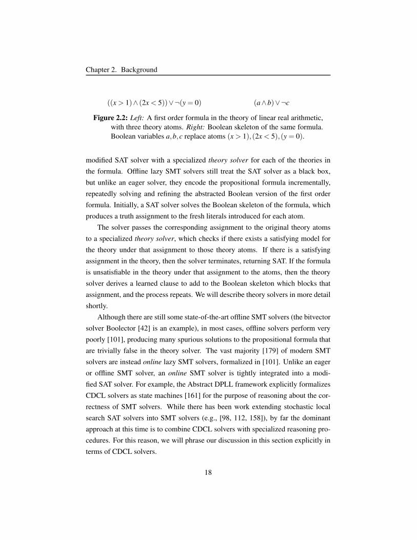
The key idea behind lazy SMT solvers is to have the solver operate on an ab-
stracted, Boolean skeleton of the original first order formula, in which each theory
atom has been swapped out for a fresh Boolean literal (see Figure 2.2). The first
lazy SMT solvers were offline [31, 72, 73]. Offline SMT solvers combine an un-
17
Chapter 2. Background
((x > 1)∧ (2x < 5))∨¬(y = 0) (a∧b)∨¬c
Figure 2.2: Left: A first order formula in the theory of linear real arithmetic,with three theory atoms. Right: Boolean skeleton of the same formula.Boolean variables a,b,c replace atoms (x > 1),(2x < 5),(y = 0).
modified SAT solver with a specialized theory solver for each of the theories in
the formula. Offline lazy SMT solvers still treat the SAT solver as a black box,
but unlike an eager solver, they encode the propositional formula incrementally,
repeatedly solving and refining the abstracted Boolean version of the first order
formula. Initially, a SAT solver solves the Boolean skeleton of the formula, which
produces a truth assignment to the fresh literals introduced for each atom.
The solver passes the corresponding assignment to the original theory atoms
to a specialized theory solver, which checks if there exists a satisfying model for
the theory under that assignment to those theory atoms. If there is a satisfying
assignment in the theory, then the solver terminates, returning SAT. If the formula
is unsatisfiable in the theory under that assignment to the atoms, then the theory
solver derives a learned clause to add to the Boolean skeleton which blocks that
assignment, and the process repeats. We will describe theory solvers in more detail
shortly.
Although there are still some state-of-the-art offline SMT solvers (the bitvector
solver Boolector [42] is an example), in most cases, offline solvers perform very
poorly [101], producing many spurious solutions to the propositional formula that
are trivially false in the theory solver. The vast majority [179] of modern SMT
solvers are instead online lazy SMT solvers, formalized in [101]. Unlike an eager
or offline SMT solver, an online SMT solver is tightly integrated into a modi-
fied SAT solver. For example, the Abstract DPLL framework explicitly formalizes
CDCL solvers as state machines [161] for the purpose of reasoning about the cor-
rectness of SMT solvers. While there has been work extending stochastic local
search SAT solvers into SMT solvers (e.g., [98, 112, 158]), by far the dominant
approach at this time is to combine CDCL solvers with specialized reasoning pro-
cedures. For this reason, we will phrase our discussion in this section explicitly in
terms of CDCL solvers.
18
Chapter 2. Background
An online lazy SMT solver consists of two components. The first, as with of-
fline lazy solvers, is a specialized theory solver (or ‘T-solver’). The second compo-
nent is a modified CDCL solver, which adds a number of hooks to interact with the
theory solver. As before, the SAT solver operates on an abstracted Boolean skele-
ton of the first order formula, φ ′. Unlike in offline solvers, an online solver does not
wait to generate a complete satisfying assignment to the Boolean formula before
checking whether the corresponding assignment to the theory atoms is satisfiable
in the theory solver, but instead calls the theory solver eagerly, as assignments to
theory literals are made in the SAT solver.
Theory solvers may support some or all of the following methods:
1. T-Propagate (M):
The most basic version of T-Propagate (also called T-Deduce) takes a com-
plete truth assignmentM to the theory atoms (for a single theory), returning
TRUE ifM is satisfiable in the theory, and FALSE otherwise.
In contrast to offline solvers, online lazy SMT solvers (typically) make calls
to T-Propagate eagerly [101], as assignments are being built in the CDCL
solver, rather than waiting for a complete satisfying assignment to be gen-
erated. In this case, T-Propagate takes a partial, rather than a complete,
assignment to the theory atoms. When operating on a partial assignment,
T-Propagate makes deductions on a best-effort basis: if it can prove that the
partial assignment is unsatisfiable, then it returns FALSE, and otherwise it
returns TRUE. By calling T-Propagate eagerly, assignments that may sat-
isfy the abstract Boolean skeleton, but which are unsatisfiable in the theory
solver, can be pruned from the CDCL solvers search space. This technique
is sometimes called early pruning.
All theory solvers must support at least this basic functionality, but some
theory solvers can do more. If M is a partial assignment, efficient theory
solvers may also be able to deduce assignments for some of the unassigned
atoms. These are truth assignments to theory literals l that must hold in all
satisfying completions ofM, writtenM =⇒T
l. Along with early pruning,
deducing unassigned theory literals may greatly prune the search space of
the solver, avoiding many trivially unsatisfiable solutions.
19
Chapter 2. Background
As with unit propagation, the CDCL solver typically continues applying unit
propagation and theory propagation until no further deductions can be made
(or the assignment is found to be UNSAT). However, there are many possible
variations on the exact implementation of theory propagation. For many
theories of interest, testing satisfiability may be very expensive; deducing
assignments for unassigned atoms may be an additional cost on top of that,
in some cases a prohibitively expensive one. Many theory solvers can only
cheaply make deductions of a subset of the possible forced assignments.
Theory solvers that make all possible deductions of unassigned literals are
called deduction complete.
There are many possible optimizations that have been explored in the lit-
erature to try to mitigate the cost of expensive theory propagation calls. A
small selection include: only calling theory propagate when one or more
theory literals have been assigned [108]; pure literal filtering [16, 39], which
can remove some redundant theory literals from M; or only calling the-
ory propagate every k unit propagation calls, rather than for every single
call [10]. A theory solver that does not directly detect implied literals can
still be used to deduce such literals by testing, for each unassigned literal
l, whether M∪¬l is unsatisfiable. This technique is known as theory
plunging[77], however, it is rarely used in practice due to its cost.
2. T-Analyze (M):
When an assignment to the theory atoms M is unsatisfiable in the theory,
then an important task for a theory solver is to find a (possibly minimal)
subset of M that is sufficient to be unsatisfiable. This unsatisfiable subset
may be called a conflict set or justification set or infeasible set; its negation (a
clause of theory literals, at least one of which must be true in any satisfying
model) may be called a theory lemma or a learned clause.
T-Analyze may always return the entire M as a conflict set; this is known
as the naıve conflict set. Unfortunately, the naıve conflict set is typically a
very poor choice, as it blocks only the exact assignment M to the theory
atoms. Conversely, it is also possible to find a (locally) minimal conflict set
through a greedy search, repeatedly dropping literals fromM and checking
20
Chapter 2. Background
if it is still unsatisfiable. However, in addition to not guaranteeing a globally
minimal conflict set, such a method is typically prohibitively expensive, es-
pecially if the theory propagate method is expensive. Finding small conflict
sets quickly is a key challenge for theory solvers.
3. T-Backtrack(level):
In many cases, efficient theory solvers maintain incremental data structures,
so that as T-Propagate (M) is repeatedly invoked, redundant computation
in the theory solver can be avoided. T-Backtrack is called when the CDCL
solver backtracks, to keep those incremental data structures in sync with the
CDCL solver’s assignments.
4. T-Decide(M):
Some theory solvers are able to heuristically suggest unassigned theory liter-
als as decisions to the SAT solver. If there are multiple theory solvers capable
of suggesting decisions, the SAT solver may need to have a way of choosing
between them.
5. T-Model(M):
Given a theory-satisfiable assignment M to the theory atoms, this method
extends M into a satisfying model to each of the (non-Boolean) variables
and function terms in the formula. Generating a concrete model may require
a significant amount of additional work on top of simply checking the sat-
isfiability of a Boolean assignment M, and so may be separated off into a
separate method to be called when the SMT solver finds a satisfying solu-
tion. In some solvers (such as Z3 [70]), models can be generated on demand
for specified subsets of the theory variables.
Writing an efficient lazy SMT solver involves finding a balance between more
expensive deduction capabilities in the theory solver and faster searches in the
CDCL solver; finding the right balance is difficult and may depend not only on
the implementation of the theory solver but also on the instances being solved. For
a more complete survey of some of the possible optimizations to CDCL solvers for
integration with lazy theory solvers, we refer readers to Chapter 6 of [179].
21
Chapter 2. Background
2.5 Related WorkIn the following chapters, we will introduce the main subject of this thesis: a gen-
eral framework for building efficient theory solvers for a special class of theories,
which we call monotonic theories. Several other works in the literature have also
introduced high-level, generic frameworks for building SMT solvers. There are
also previous constraint solvers which exploit monotonicity. Here, we briefly sur-
vey some of the most closely related works. Additionally, the applications and
specific theories we consider later in this thesis (Chapters 5, 6, 7, and 8) also have
their own, subject-specific literature reviews, and we describe related work in the
relevant chapters.
There have been a number of works proposing generic SMT frameworks that
are not specialized for any particular class of first order theories. The best known
of these are the DPLL(T) and Abstract DPLL frameworks [101, 161]. Addition-
ally, an approach based on extending simplex into a generic SMT solver method
is described in [111]. These frameworks have in common that they are not spe-
cific to the class of theories being supported by the SMT solver; the techniques de-
scribed in them apply generically to all (quantifier free, first order) theories. There-
fore, the work in this thesis could be considered to be an instance of the DPLL(T)
framework. However, these high-level frameworks do not articulate any concept
of monotonic theories, and provide no guidance for exploiting their properties.
As we will see in Chapters 5 and 6, some of our most successful examples of
monotonic theories are graph theoretic. Two recent works have proposed generic
frameworks for extending SMT solvers with support for graph properties:
The first of the two, [220], proposed MathCheck, which extends an SMT solver
by combining it with an external symbolic math library (such as SAGE [189]). This
allows the SMT solver great flexibility in giving it access to a wide set of operations
that can be specified by users in the language of the symbolic math library. They
found that they were able to prove bounded cases of several discrete mathemati-
cal theorems using this approach. Unfortunately, their approach is fundamentally
an off-line, lazy SMT integration, and as such represents a extremal point in the
expressiveness-efficiency trade-off: their work can easily support many previously
unsupported theories (including theories that are non-monotonic), however, those
22

Chapter 2. Background
solvers are typically much less efficient than SMT solvers with dedicated support
for the same theories.
The second of the two, [133], introduced SAT-to-SAT. Like [220], they de-
scribe an off-line, lazy SMT solver. However, rather than utilizing an external math
library to implement the theory solver, they utilize a second SAT solver to imple-
ment the theory solver. Further, they negate the return value of that second SAT
solver, essentially treating it as solving a negated, universally quantified formula.
Their approach is similarly structured to the 2QBF solvers proposed in [172] and
[185]. Like MathCheck, SAT-to-SAT is not restricted to monotonic theories. How-
ever, SAT-to-SAT requires encoding the supported theory in propositional logic,
and suffers a substantial performance penalty compared to our approach (for the
theories that both of our solvers support).
One of the main contributions of this thesis is our framework for interpreted
monotonic functions in SMT solving. Although there has been work addressing
uninterpreted monotonic functions in SMT solvers [23], we believe that no previ-
ous work has specifically addressed exploiting interpreted monotonic functions in
SMT solvers.
Outside of SAT and SMT solving, other techniques in formal methods have
long considered monotonicity. In the space of non-SMT based constraint solvers,
two examples include [213], who proposed a generic framework for building CSP
solvers for monotonic constraints; and interval arithmetic solvers, which are often
designed to take advantage of monotonicity directly (see, e.g., [122] for a sur-
vey). Neither of these techniques directly extend to SMT solvers, nor have they
been applied to the monotonic theories that we consider in this thesis. Addition-
ally, several works have exploited monotonicity within SAT/SMT-based model-
checkers [43, 96, 115, 142].
23
Chapter 3
SAT Modulo Monotonic Theories
Our interest in this work is to develop tools for building solvers for finite-domain
theories in which all predicates and functions are monotonic — i.e., they consis-
tently increase (or consistently decrease) as their arguments increase. These are
the finite monotonic theories.1 In this chapter, we formally define monotonic pred-
icates (Section 3.1) and monotonic theories (Section 3.2).
While this notion of a finite monotonic theory may initially seem limited, we
will show that such theories are natural fits for describing many useful properties
of discrete, finite structures, such as graphs (Chapter 5) and automata (Chapters
8). Moreover, we have found that many useful finite monotonic theories can be
efficiently solved in practice using a common set of simple techniques for building
lazy SMT theory solvers (Section 2.4). We will describe these techniques — the
SAT Modulo Monotonic Theories (SMMT) framework — in Chapter 4.
3.1 Monotonic PredicatesConceptually, a (positive) monotonic predicate P is one for which if P(x) holds,
and y≥ x, then P(y) holds. An example of a monotonic predicate is IsPositive(x) :
R 7→ T,F, which takes a single real-valued argument x, and returns TRUE iff
x > 0. An example of a non-monotonic predicate is IsPrime(x). Formally:
1To forestall confusion, note that our concept of a ‘monotonic theory’ here has no direct relation-ship to the concept of monotonic/non-monotonic logics.
24
Chapter 3. SAT Modulo Monotonic Theories
Definition 1 (Monotonic Predicate). A predicate P: σ1,σ2, . . .σn 7→ T,F,over sorts σi is monotonic iff, for each i in 1..n, the following holds:
Positive monotonic in argument i:∀s1 . . .sn,∀x≤ y : P(. . . ,si−1,x,si+1, . . .)→ P(. . . ,si−1,y,si+1, . . .)
—or—
Negative monotonic in argument i:∀s1 . . .sn,∀x≤ y : ¬P(. . . ,si−1,x,si+1, . . .)→¬P(. . . ,si−1,y,si+1, . . .)
We will say that a predicate P is positive monotonic in argument i if ∀s1 . . .sn,
∀x≤ y : P(. . . ,si−1,x,si+1, . . .)→ P(. . . ,si−1,y,si+1, . . .); we will say that P is
negative monotonic in argument i if ∀s1 . . .sn,∀x≤ y :¬P(. . . ,si−1,x,si+1, . . .)→¬P(. . . ,si−1,y,si+1, . . .). Notice that although P must be monotonic in all of
its arguments, it may be positive monotonic in some, and negative monotonic
in others.
Notice that Definition 1 does not specify whether ≤ forms a total or a partial
order. In this work, we will typically assume total orders, though we consider
extensions to support partial orders in Section 4.4.
This work is primarily concerned with monotonic predicates over finite sorts
(such as Booleans and bit vectors); we refer to such predicates as finite monotonic
predicates. Two closely related special cases of finite monotonic predicates de-
serve attention: monotonic predicates over Booleans, and monotonic predicates
over powerset lattices. Formally, we define Boolean monotonic predicates as:
25
Chapter 3. SAT Modulo Monotonic Theories
Definition 2 (Boolean Monotonic Predicate). A predicate P: T,Fn 7→ T,Fis Boolean monotonic iff, for each i in 1..n, the following holds:
Positive monotonic in argument i:∀s1 . . .sn : P(. . . ,si−1,F,si+1, . . .)→ P(. . . ,si−1,T,si+1, . . .)
—or—
Negative monotonic in argument i:∀s1 . . .sn : ¬P(. . . ,si−1,F,si+1, . . .)→¬P(. . . ,si−1,T,si+1, . . .)
As an example of a Boolean monotonic predicate, consider the pseudo-Boolean
inequality ∑n−1i=0 cibi ≥ cn, with each bi a variable in T,F, and each ci a non-
negative integer constant. This inequality can be modeled as a positive Boolean
monotonic predicate P over the Boolean arguments bi, such that P is TRUE iff the
inequality is satisfied.
This definition of monotonicity over Booleans is closely related to a definition
of monotonic predicates of powerset lattices found in [41] and [145]. Given a
set S, [41] defines a predicate P : 2S 7→ T,F to be monotonic if P(Sx)→ P(Sy)
for all Sx ⊆ Sy.2 Slightly generalizing on that definition, we define a monotonic
predicate over set arguments as:
Definition 3 (Set-wise Monotonic Predicate). Given sets S1,S2 . . .Sn a pred-
icate P: 2S1 ,2S2 . . .2Sn 7→ T,F, is monotonic iff, for each i in 1..n, the
following holds:
Positive monotonic in argument i:∀s1 . . .sn,∀sx ⊆ sy : P(. . . ,si−1,sx,si+1, . . .)→ P(. . . ,si−1,sy,si+1, . . .)
—or—
Negative monotonic in argument i:∀s1 . . .sn,∀sx ⊆ sy : ¬P(. . . ,si−1,sx,si+1, . . .)→¬P(. . . ,si−1,sy,si+1, . . .)
2Actually, [41] poses a slightly stronger requirement, requiring that P(S) must hold. We relaxthis requirement, in addition to generalizing their definition to support multiple arguments of bothpositive and negative monotonicity.
26
Chapter 3. SAT Modulo Monotonic Theories
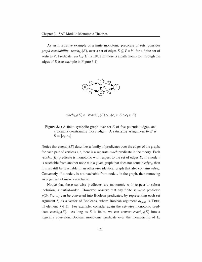
As an illustrative example of a finite monotonic predicate of sets, consider
graph reachability: reachs,t(E), over a set of edges E ⊆ V ×V , for a finite set of
vertices V . Predicate reachs,t(E) is TRUE iff there is a path from s to t through the
edges of E (see example in Figure 3.1).
01e0
2e1
e2 3e3
e4
reach0,3(E)∧¬reach1,3(E)∧¬(e0 ∈ E ∧ e1 ∈ E)
Figure 3.1: A finite symbolic graph over set E of five potential edges, anda formula constraining those edges. A satisfying assignment to E isE = e1,e4.
Notice that reachs,t(E) describes a family of predicates over the edges of the graph:
for each pair of vertices s, t, there is a separate reach predicate in the theory. Each
reachs,t(E) predicate is monotonic with respect to the set of edges E: if a node v
is reachable from another node u in a given graph that does not contain edgei, then
it must still be reachable in an otherwise identical graph that also contains edgei.
Conversely, if a node v is not reachable from node u in the graph, then removing
an edge cannot make v reachable.
Notice that these set-wise predicates are monotonic with respect to subset
inclusion, a partial-order. However, observe that any finite set-wise predicate
p(S0,S1, . . .) can be converted into Boolean predicates, by representing each set
argument Si as a vector of Booleans, where Boolean argument bS(i, j) is TRUE
iff element j ∈ Si. For example, consider again the set-wise monotonic pred-
icate reachs,t(E). As long as E is finite, we can convert reachs,t(E) into a
logically equivalent Boolean monotonic predicate over the membership of E,
27
Chapter 3. SAT Modulo Monotonic Theories
reachs,t,E(edge1,edge2,edge3, . . .), where the Boolean arguments edgei define
which edges (via some mapping to the fixed set of possible edges E) are included
in the graph.
This transformation of set-wise predicates into Boolean predicates will prove to
be advantageous later, as the Boolean formulation is totally-ordered (with respect
to each individual Boolean argument), whereas the set-wise formulation is only
partially ordered. As we will discuss in Section 4.4, the SMMT framework —
while applicable also to partial orders — works better for total orders. Below, we
assume that monotonic predicates of finite sets are always translated into logically
equivalent Boolean monotonic predicates, unless otherwise stated.
3.2 Monotonic TheoriesMonotonic predicates and functions — finite or otherwise — are common in the
SMT literature, but in most cases are considered alongside collections of non-
monotonic predicates and functions. For example, the inequality x+ y > z, with
x,y,z real-valued, is an example of an infinite domain monotonic predicate in the
theory of linear arithmetic (positive monotonic in x,y, and negative monotonic in
z). However, the theory of linear arithmetic — as with most common theories —
can also express non-monotonic predicates (e.g., x = y, which is not monotonic in
either argument).
We introduce the restricted class of finite monotonic theories, which are theo-
ries over finite domain sorts, in which all predicates and functions are monotonic.
Formally, we define a finite monotonic theory as:
Definition 4 (Finite Monotonic Theory). A theory T with signature Σ is finite
monotonic if and only if:
1. All sorts in Σ have finite domains;
2. all predicates in Σ are monotonic; and
3. all functions in Σ are monotonic.
As is common in the context of SMT solving, we consider only decidable,
28
Chapter 3. SAT Modulo Monotonic Theories
quantifier-free, first-order theories. All predicates in the theory must be mono-
tonic; atypically for SMT theories, monotonic theories do not include equality (as
equality is non-monotonic). Rather, as each sort σ ∈ T is ordered, we assume the
presence of comparison predicates in T : <,≤,≥,>, over σ×σ . Unlike the equal-
ity predicate, the comparison predicate is monotonic, and we will take advantage
of this property subsequently.
Above, we described two finite monotonic predicates: a predicate of pseudo-
Boolean comparisons, and a predicate of finite graph reachability. A finite mono-
tonic theory might collect together several monotonic predicates that operate over
one or more sorts. For example, many common graph properties are monotonic
with respect to the edges in the graph, and a finite monotonic theory of graphs
might include in its signature several predicates, including the above mentioned
reachs,t(E), as well as additional monotonic predicates such as acyclic(E), which
evaluates to TRUE iff edges E do not contain a cycle, or planar(E) which evaluates
to TRUE iff edges E induce a planar graph. 3
Although almost all theories considered in the SMT literature are non-
monotonic, particularly as most theories implicitly include the equality predicate,
we will show that many useful properties — including many properties that have
not previously had practical support in SAT solvers — can be modeled as mono-
tonic finite theories, and solved efficiently. Moreover, we will show in Chapter
4, that building high-performance SMT solvers for such theories is simple and
straightforward. Subsequently, in Chapters 5, 7, and 8 of this thesis, we will
demonstrate state-of-the-art implementations of lazy SMT solvers for several im-
portant finite monotonic theories that previously had poor support in SAT solvers.
3In previous work [33], we considered the special case of a Boolean monotonic theory, in whichthe only sort in the theory is Boolean (and hence all monotonic predicates are Boolean monotonicpredicates). In this thesis, the notion of a Boolean monotonic theory is subsumed by the more generalnotion of a finite monotonic theory.
29
Chapter 4
A Framework for SAT ModuloMonotonic Theories
This chapter introduces a set of techniques — the SAT Modulo Monotonic The-
ories (SMMT) framework — taking advantage of the special properties of finite
monotonic theories in order to create efficient SMT solvers, by providing efficient
theory propagation and improving upon naıve conflict analysis.1
Many successful SMT solvers follow the lazy SMT design [70, 179], in which
a SAT solver is combined with a set of theory solvers (or T-solvers), which are
responsible for reasoning about assignments to theory atoms (see Section 2.4 for
more details about lazy SMT solvers).
While T-solvers may support more complex interfaces, every T-solver must at
minimum support two procedures:
1. T-Propagate (M), which takes a (possibly partial) assignment M to the
theory atoms, and returns FALSE if it can prove that M is unsatisfiable in
the theory, and TRUE if it could not proveM to be unsatisfiable. 2
2. T-Analyze (M), which, given an unsatisfiable assignment to the theory liter-
alsM, returns a subset (a conflict set) that is also unsatisfiable.3
1This chapter describes the SMMT framework at a high-level; we refer readers to Appendix Afor a discussion of some of the practical considerations required for an efficient implementation.
2T-Propagate is sometimes referred to as T-Deduce in the literature.3T-Analyze is sometimes referred to as conflict or justification set derivation, or as lemma learning
30
Chapter 4. A Framework for SAT Modulo Monotonic Theories
The SMMT framework provides a pattern for implementing these two procedures.
In principle, T-Propagate is only required to return FALSE when a complete
assignment to the theory atoms is unsatisfiable (returning TRUE on partial assign-
ments), and T-Analyze may always return the naıve conflict set (i.e., it may return
the entire assignmentM as the conflict set). However, efficient T-Propagate imple-
mentations typically support checking the satisfiability of partial assignments (al-
lowing the SAT solver to prune unsatisfiable branches early). Efficient T-Propagate
implementations are often also able to derive unassigned literals l that are implied
by a partial assignment M, such that T ∪M |= l. Any derived literals l can be
added toM, and returned to the SAT solver to extend the current assignment. Effi-
cient implementations of T-Analyze typically make an effort to return small (some-
times minimal) unsatisfiable subsets as conflict sets. Although there are many other
implementation details that can impact the performance of a theory solver (such as
the ability for the theory solver to be applied efficiently as an assignment is in-
crementally built up or as the solver backtracks), the practical effectiveness of a
lazy SMT solver depends on fast implementations of T-Propagate and T-Analyze.
This implies a design trade-off, where more powerful deductive capabilities in the
theory solver must be balanced against faster execution time.
In Sections 4.1 and 4.2, we show how efficient theory propagation and conflict
analysis can be implemented for finite monotonic theories. The key insight is to
observe that many predicates have known, efficient algorithms for evaluating their
truth value when given fully specified inputs, but not for partially specified or sym-
bolic inputs.4 For example, given a concretely specified graph, one can find the set
of nodes reachable from u simply using any standard graph reachability algorithm,
such as depth-first-search.
Given only a procedure for computing the truth-values of the monotonic pred-
icates P from complete assignments, we will show how we can take advantage of
the properties of a monotonic theory to form a complete decision procedure for any
or clause learning (in which case the method returns a clause representing the negation of a conflictset).
4Evaluating a function given a partially specified or symbolic input is typically more challengingthan evaluating a function on a fully specified, concrete input, as the return value may be a set ofpossible values, or a formula, rather than a concrete value. Additionally, evaluating a function on apartial or symbolic assignment may entail an expensive search over the remaining assignment space.
31
Chapter 4. A Framework for SAT Modulo Monotonic Theories
finite monotonic theory, and, further, we will show that in many cases the resulting
theory solver performs much better than preexisting solvers in practice.
For clarity, in Sections 4.1 and 4.2 we initially describe how to apply the-
ory propagation and conflict analysis for the special case of function-free, totally-
ordered finite monotonic theories. These are finite monotonic theories that have
no functions in their signature, aside from predicates (of any arity), and aside from
constant (arity-0) functions, and for which every sort has a total order relation-
ship (rather than a partial order relationship). Subsequently, we relax these restric-
tions to support formulas with compositions of positive and negative monotonic
functions (Section 4.3), and to support finite sorts that are only partially-ordered
(Section 4.4).
4.1 Theory Propagation for Finite Monotonic TheoriesFirst, we show how efficient theory propagation can be performed for function-
free, totally ordered, finite monotonic theories. Consider a theory with a monotonic
predicate P(x0,x1, . . .), with xi of finite sort σ . Let σ be totally ordered, over the
finite domain of constants σ⊥,σ1, . . . ,σ>, with σ⊥ ≤ σ1 ≤ . . .≤ σ>.
In Algorithm 3, we describe the simplest version of our procedure for perform-
ing theory propagation on partial assignments for function-free, totally-ordered fi-
nite monotonic theories. For simplicity, we also assume for the moment that all
predicates are positive monotonic in all arguments.5
Algorithm 3 is straightforward. Intuitively, it simply constructs conservative
upper and lower bounds (x+,x−) for each variable x, and then evaluates each predi-
cate on those upper and lower bounds. Since the predicates are positive monotonic,
if p(x−) evaluates to TRUE, then p(x), for any possible assignment of x≥ x−, must
also evaluate to TRUE. Therefore, if p(x−) evaluates to TRUE, we can conclude
that p(x) must be TRUE in any satisfying completion of the partial assignmentM.
Similarly, if p(x+) evaluates to FALSE, then p(x) must be FALSE in any satisfying
completion ofM. The extension to multiple arguments is obvious, and presented
in Algorithm 3; we discuss further extensions in Sections 4.3 and 4.4.
5In the special case of a function-free Boolean monotonic theory, in which all predicates arerestricted to purely Boolean arguments, Algorithm 3 can be simplified slightly by reducing compar-isons to truth assignments (e.g., (x < 1)≡ ¬x, if x ∈ T,F.).
32
Chapter 4. A Framework for SAT Modulo Monotonic Theories
Because x− and x+ are constants, rather than symbolic expressions, evaluating
p(x−) or p(x+) does not require any reasoning about p over symbolic arguments.
As such, so long as one has any algorithm for computing predicate p on con-
crete inputs (not symbolic), one can plug that algorithm into Algorithm 3 to get
a complete theory propagation procedure. In the typical case that computing p is
well-studied, one has the freedom to use any existing algorithm for computing p
in order to implement theory propagation and theory deduction — so long as p is
monotonic. For example, if p is the graph reachability predicate we considered in
Chapter 3, one can directly apply depth-first-search — or any other standard graph
reachability algorithm from the literature — to evaluate p on the under and over
approximations of its graph.
In other words, for finite monotonic theories, the same algorithms that can be
used to check the truth value of a predicate in a witnessing model (i.e., a complete
assignment of every atom and also of each variable to a constant value) can also
be used to perform theory propagation and deduction (and, we will demonstrate
experimentally, does so very efficiently in practice). This is in contrast to the usual
case in lazy SMT solvers, in which the algorithms capable of evaluating the satisfi-
ability of partial assignments may bear little resemblance to algorithms capable of
evaluating a witness — typically, the latter is trivial, while the former may be very
complex.
The distinction here is well-illustrated by any of the widely supported arith-
metic theories, such as difference logic, linear arithmetic, or integer arithmetic.
Checking a witness for any of these three arithmetic theories is trivial, requiring
linear time in the formula size. In contrast, finding efficient techniques for check-
ing the satisfiability of a (partial or complete) assignment to the atoms in any of
these three theories bears little resemblance to witness checking — for example,
typical linear arithmetic theory solvers check satisfiability of partial assignments
using variations of the simplex algorithm(e.g., [80]), while difference logic solvers
may perform satisfiability checking on partial assignments by testing for cycles in
an associated constraint graph [144, 200]).
The correctness of Algorithm 3 relies on Lemma 4.1.1, which relates models
of atoms which are comparisons to constants, and models of atoms of positive
monotonic predicates. We observe that the following lemma holds:
33
Chapter 4. A Framework for SAT Modulo Monotonic Theories
Lemma 4.1.1 (Model Monotonicity). Let MA be an assignment only to atoms
comparing variables to constants.6 For any given variable x with sort σ , any two
constants σi ≤ σ j, and any positive monotonic predicate atom p:7
MA∪(x≥ σi)=⇒T
p → MA∪(x≥ σ j)=⇒T
p (4.1)
MA∪(x≤ σ j)=⇒T¬p → MA∪(x≤ σi)=⇒
T¬p (4.2)
A proof of this lemma can be found in Appendix C.1; the lemma easily gener-
alizes for predicates of mixed positive and negative monotonicity.
Algorithm 3 constructs, for each variable x, an over-approximation constant x+,
and an under-approximation constant x−. It also constructs an under-approximate
assignmentM−A in which for each variable x, (x≤ x−)∈M−
A and (x≥ x−)∈M−A ,
forcing the evaluation of x to be exactly x− inM−A . Similarly, Algorithm 3 creates
an over-approximate model M+A forcing each variable x to x+. Note that both
of these assignments contain only atoms that compare variables to constants, and
hence match the prerequisites of Lemma 4.1.1.
By Lemma 4.1.1, if M−A =⇒
Tp, then M =⇒
Tp. Also by Lemma 4.1.1, if
M+A =⇒
T¬p, thenM =⇒
T¬p. By evaluating each predicate inM−
A andM+A ,
Algorithm 3 safely under- and over-approximates the truth value of each p inM,
using only two concrete evaluations of each predicate atom.
Lemma 4.1.1 guarantees that Algorithm 3 returns FALSE only if T |= ¬M;
however, it does not guarantee that Algorithm 3 returns FALSE for all unsatisfiable
partial assignments. In the case whereMA is a complete and consistent assignment
to every variable x, we have x− = x+ for each x (and henceM−A =M+
A ), and so for
each p, it must be the case that either p(x−0 ,x−1 , . . .) 7→ TRUE or p(x+0 ,x
+1 , . . .) 7→
FALSE. Therefore, ifMA is a complete assignment, Algorithm 3 returns FALSE if
and only if T |= ¬M.
6MA contains only atoms of comparisons of variables to constants. Comparisons between twonon-constant variables are treated as monotonic predicates, and are not included in MA. Also, forsimplicity of presentation (but without loss of generality), we assume that all comparison atomsin MA are normalized to the form (x ≥ σi), or (x ≤ σi). In the special case that atom (x < σ⊥)or (x > σ>) (or, equivalently, theory literals ¬(x ≥ σ⊥),¬(x ≤ σ>)) are in MA, the assignment istrivially unsatisfiable, but cannot be normalized to inclusive comparisons.
7Where A =⇒T
B is shorthand for ‘(A∧¬B) is unsatisfiable in theory T ’.
34
Chapter 4. A Framework for SAT Modulo Monotonic Theories
Algorithm 3 is guaranteed to be complete only whenM+A =M−
A , which is only
guaranteed to occur when M is a complete assignment to the comparison atoms
(but not necessarily a complete assignment to the theory predicates). If M+A 6=
M−A , then it is possible for Algorithm 3 to fail to deduce conflicts, or unassigned
atoms, that are in fact implied by the theory (in the terminology of Section 2.4,
Algorithm 3 is not deduction complete). For example, Algorithm 3 may fail to
deduce non-comparison atom p1 from a second non-comparison atom p0 in the
case that p0 =⇒T
p1.
For this reason, Algorithm 3 must be paired with a procedure for searching the
space of possible assignments to A in order to form a complete decision procedure.
For finite domain theories, this does not pose a problem, as one can either perform
internal case splitting in the theory solver, or simply encode the space of possible
assignments to each variable in fresh Boolean variables (for example, as a unary
or binary encoding over the space of possible values in the finite domain of σ ), al-
lowing the SAT solver to enumerate that (finite) space of assignments (an example
of splitting-on-demand [28]). In practice, we have always chosen the latter option,
and found it to work well across a wide range of theories.
As we will show in subsequent chapters, Algorithm 3, when combined with an
appropriate conflict analysis procedure, is sufficient to build efficient solvers for a
wide set of useful theories.
Returning to our earlier example from Section 3.1 of a pseudo-Boolean
constraint predicate ∑n−1i=0 cibi ≥ cn, with Boolean arguments bi and constants
c0, . . .cn, Algorithm 3 could be implemented as shown in Algorithm 5.
Our presentation of Algorithm 3 above is stateless: the UpdateBounds sec-
tion recomputes the upper- and lower-approximation assignments at each call to
T-Propagate. In a practical implementation, this would be enormously wasteful, as
the under- and over-approximate assignments will typically be expected to change
only in small ways between theory propagate calls. In a practical implementation,
one would store the upper- and lower-approximation assignments between calls to
T-Propagate, and only alter them as theory literals are assigned or unassigned in
M. A practical, stateful implementation of Algorithm 3 is described in more detail
in Appendix A.
For example, the pseudo-code in Algorithm 5 is a nearly complete representa-
35
Chapter 4. A Framework for SAT Modulo Monotonic Theories
tion of the actual implementation of theory propagation for pseudo-Boolean con-
straints that we have implemented in our SMT solver, with the only difference be-
ing that in our implementation we maintain running under- and over-approximate
sums (∑n−1i=0 cib−i ,∑
n−1i=0 cib+i ), updated each time a theory literal is assigned or unas-
signed in the SAT solver, rather than re-calculating them at each T-Propagate call.
36
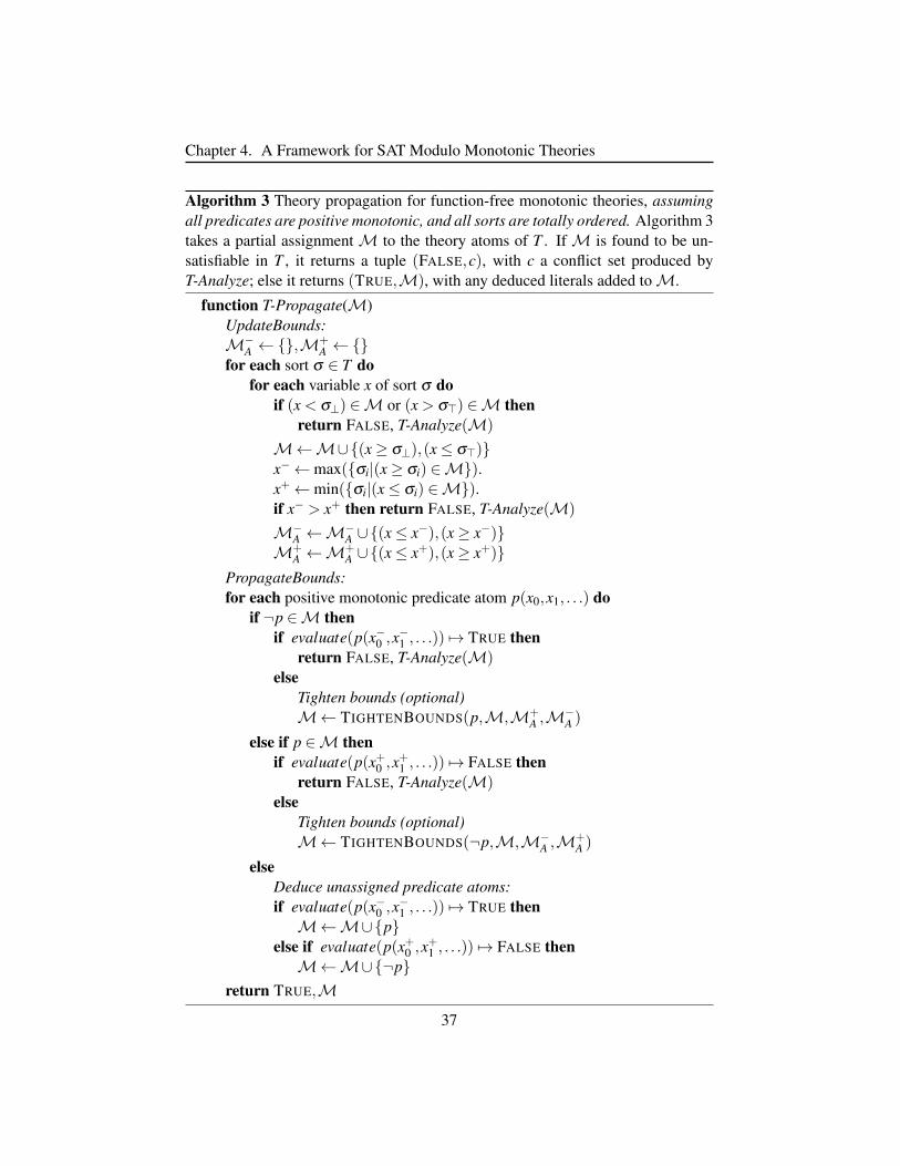
Chapter 4. A Framework for SAT Modulo Monotonic Theories
Algorithm 3 Theory propagation for function-free monotonic theories, assumingall predicates are positive monotonic, and all sorts are totally ordered. Algorithm 3takes a partial assignmentM to the theory atoms of T . If M is found to be un-satisfiable in T , it returns a tuple (FALSE,c), with c a conflict set produced byT-Analyze; else it returns (TRUE,M), with any deduced literals added toM.
function T-Propagate(M)UpdateBounds:M−
A ←,M+A ←
for each sort σ ∈ T dofor each variable x of sort σ do
if (x < σ⊥) ∈M or (x > σ>) ∈M thenreturn FALSE, T-Analyze(M)
M←M∪(x≥ σ⊥),(x≤ σ>)x−←max(σi|(x≥ σi) ∈M).x+←min(σi|(x≤ σi) ∈M).if x− > x+ then return FALSE, T-Analyze(M)
M−A ←M
−A ∪(x≤ x−),(x≥ x−)
M+A ←M
+A ∪(x≤ x+),(x≥ x+)
PropagateBounds:for each positive monotonic predicate atom p(x0,x1, . . .) do
if ¬p ∈M thenif evaluate(p(x−0 ,x
−1 , . . .)) 7→ TRUE then
return FALSE, T-Analyze(M)else
Tighten bounds (optional)M← TIGHTENBOUNDS(p,M,M+
A ,M−A )
else if p ∈M thenif evaluate(p(x+0 ,x
+1 , . . .)) 7→ FALSE then
return FALSE, T-Analyze(M)else
Tighten bounds (optional)M← TIGHTENBOUNDS(¬p,M,M−
A ,M+A )
elseDeduce unassigned predicate atoms:if evaluate(p(x−0 ,x
−1 , . . .)) 7→ TRUE then
M←M∪pelse if evaluate(p(x+0 ,x
+1 , . . .)) 7→ FALSE then
M←M∪¬preturn TRUE,M
37

Chapter 4. A Framework for SAT Modulo Monotonic Theories
Algorithm 4 TIGHTENBOUNDS is an optional routine which may be called byimplementations of Algorithm 3. TIGHTENBOUNDS takes a predicate p that hasbeen assigned a truth value, and performs a search over the arguments xi of p tofind tighter bounds on xi that can be added toM.
function TIGHTENBOUNDS(p(x0,x1, . . . ,xn),M,M+A ,M
−A )
for each x0 . . .xn doif p is positive monotonic in argument i (which has sort σ ) then
for each y ∈ σ ,M−A [xi]< y≤M+
A [xi] doif evaluate(p(. . . ,M−
A [xi−1],y,M−A [xi+1], . . .)) 7→ TRUE then
M←M∪(xi < y)else
for each y ∈ σ ,M+A [xi]> y≥M−
A [xi] doif evaluate(p(. . . ,M+
A [xi−1],y,M+A [xi+1], . . .)) 7→ TRUE then
M←M∪(xi > y)returnM
38
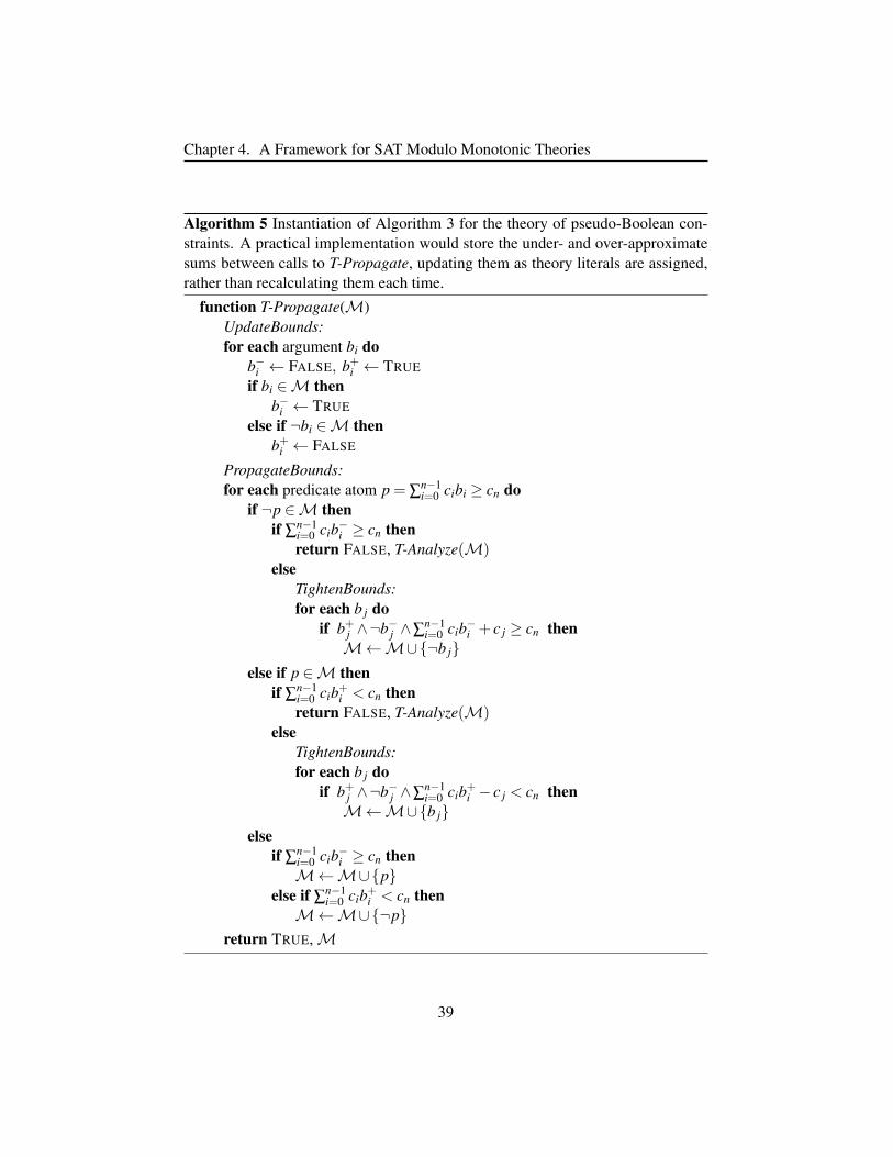
Chapter 4. A Framework for SAT Modulo Monotonic Theories
Algorithm 5 Instantiation of Algorithm 3 for the theory of pseudo-Boolean con-straints. A practical implementation would store the under- and over-approximatesums between calls to T-Propagate, updating them as theory literals are assigned,rather than recalculating them each time.
function T-Propagate(M)UpdateBounds:for each argument bi do
b−i ← FALSE, b+i ← TRUE
if bi ∈M thenb−i ← TRUE
else if ¬bi ∈M thenb+i ← FALSE
PropagateBounds:for each predicate atom p = ∑
n−1i=0 cibi ≥ cn do
if ¬p ∈M thenif ∑
n−1i=0 cib−i ≥ cn thenreturn FALSE, T-Analyze(M)
elseTightenBounds:for each b j do
if b+j ∧¬b−j ∧∑n−1i=0 cib−i + c j ≥ cn then
M←M∪¬b jelse if p ∈M then
if ∑n−1i=0 cib+i < cn thenreturn FALSE, T-Analyze(M)
elseTightenBounds:for each b j do
if b+j ∧¬b−j ∧∑n−1i=0 cib+i − c j < cn then
M←M∪b jelse
if ∑n−1i=0 cib−i ≥ cn thenM←M∪p
else if ∑n−1i=0 cib+i < cn then
M←M∪¬preturn TRUE,M
39
Chapter 4. A Framework for SAT Modulo Monotonic Theories
4.2 Conflict Analysis for Finite Monotonic TheoriesIn Section 4.1, we described a technique for theory propagation in function-free,
totally-ordered finite monotonic theories. As discussed at the opening of this chap-
ter, the other function that efficient SMT solvers must implement is T-Analyze,
which takes a partial assignmentM that is unsatisfiable in theory T , and returns a
subset ofM (a ‘conflict set’) which remains unsatisfiable. Ideally, this conflict set
will be both small, and efficient to derive.
All SMT solvers have the option of returning the naıve conflict set, which is just
to return the entireM as the conflict set. However, for the special case of conflicts
derived by Algorithm 3, we describe an improvement upon the naıve conflict set,
which we call the default monotonic conflict set. So long as Algorithm 3 is used,
returning the default monotonic conflict set is always an option (and is never worse
than returning the naıve monotonic conflict set).
While in many cases we have found that theory specific reasoning allows one
to find even better conflict sets than this default monotonic conflict set, in some
cases, including the theory of pseudo-Booleans described in Algorithm 5, as well
as some of the predicates mentioned in subsequent chapters, our implementation
does in fact fall back on the default monotonic conflict set.
We describe our algorithm for deriving a default monotonic conflict set in
Algorithm 6. The first for-loop of Algorithm 6 simply handles the trivial conflicts
that can arise when building the over- and under-approximations of each variable
x+,x− in Algorithm 3 (for example, ifM is inconsistent with the total order rela-
tion of σ ); these cases are all trivial and self-explanatory.
In the last 5 lines, Algorithm 6 deals with conflicts in which the under- or
over-approximations x−,x+ are in conflict with assignment inM of a single pred-
icate atom, p. Consider a predicate atom p(x0,x1), with p positive monotonic in
each argument. Algorithm 3 can derive a conflict involving p in one of only two
cases: Either p(x+0 ,x+1 ) evaluates to FALSE, when p(x0,x1) is assigned TRUE in
M, or p(x−0 ,x−1 ) evaluates to TRUE, when p(x0,x1) is assigned FALSE inM. In
the first case, a sufficient conflict set can be formed from just the literals in Mused to set the upper bounds x+0 ,x
+1 , . . . (along with the conflicting predicate literal
p(x0,x1)). In the second case, only the atoms of M that were used to form the
40
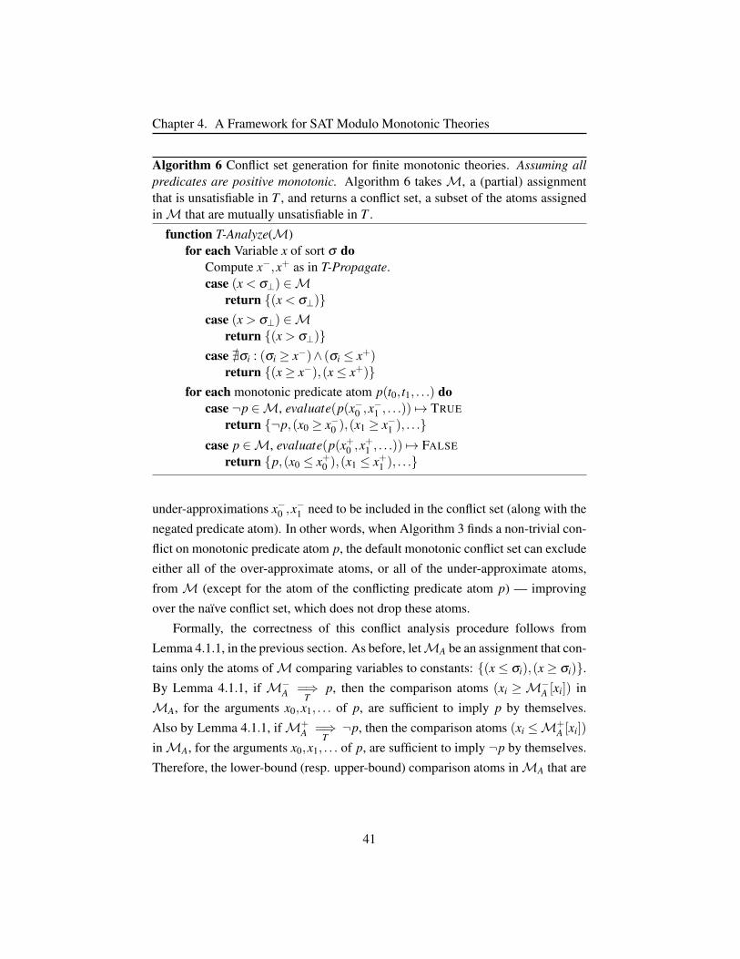
Chapter 4. A Framework for SAT Modulo Monotonic Theories
Algorithm 6 Conflict set generation for finite monotonic theories. Assuming allpredicates are positive monotonic. Algorithm 6 takes M, a (partial) assignmentthat is unsatisfiable in T , and returns a conflict set, a subset of the atoms assignedinM that are mutually unsatisfiable in T .
function T-Analyze(M)for each Variable x of sort σ do
Compute x−,x+ as in T-Propagate.case (x < σ⊥) ∈M
return (x < σ⊥)case (x > σ⊥) ∈M
return (x > σ⊥)case @σi : (σi ≥ x−)∧ (σi ≤ x+)
return (x≥ x−),(x≤ x+)for each monotonic predicate atom p(t0, t1, . . .) do
case ¬p ∈M, evaluate(p(x−0 ,x−1 , . . .)) 7→ TRUE
return ¬p,(x0 ≥ x−0 ),(x1 ≥ x−1 ), . . .case p ∈M, evaluate(p(x+0 ,x
+1 , . . .)) 7→ FALSE
return p,(x0 ≤ x+0 ),(x1 ≤ x+1 ), . . .
under-approximations x−0 ,x−1 need to be included in the conflict set (along with the
negated predicate atom). In other words, when Algorithm 3 finds a non-trivial con-
flict on monotonic predicate atom p, the default monotonic conflict set can exclude
either all of the over-approximate atoms, or all of the under-approximate atoms,
from M (except for the atom of the conflicting predicate atom p) — improving
over the naıve conflict set, which does not drop these atoms.
Formally, the correctness of this conflict analysis procedure follows from
Lemma 4.1.1, in the previous section. As before, letMA be an assignment that con-
tains only the atoms ofM comparing variables to constants: (x≤ σi),(x≥ σi).By Lemma 4.1.1, if M−
A =⇒T
p, then the comparison atoms (xi ≥M−A [xi]) in
MA, for the arguments x0,x1, . . . of p, are sufficient to imply p by themselves.
Also by Lemma 4.1.1, ifM+A =⇒
T¬p, then the comparison atoms (xi ≤M+
A [xi])
inMA, for the arguments x0,x1, . . . of p, are sufficient to imply ¬p by themselves.
Therefore, the lower-bound (resp. upper-bound) comparison atoms inMA that are
41
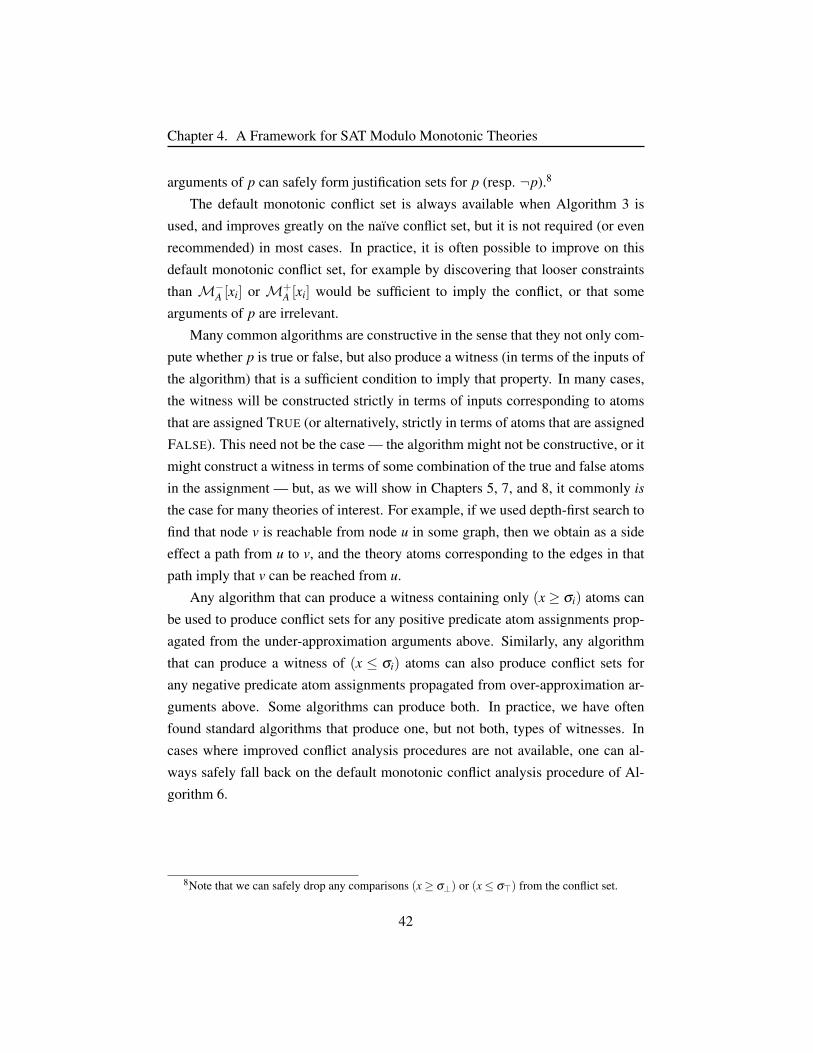
Chapter 4. A Framework for SAT Modulo Monotonic Theories
arguments of p can safely form justification sets for p (resp. ¬p).8
The default monotonic conflict set is always available when Algorithm 3 is
used, and improves greatly on the naıve conflict set, but it is not required (or even
recommended) in most cases. In practice, it is often possible to improve on this
default monotonic conflict set, for example by discovering that looser constraints
than M−A [xi] or M+
A [xi] would be sufficient to imply the conflict, or that some
arguments of p are irrelevant.
Many common algorithms are constructive in the sense that they not only com-
pute whether p is true or false, but also produce a witness (in terms of the inputs of
the algorithm) that is a sufficient condition to imply that property. In many cases,
the witness will be constructed strictly in terms of inputs corresponding to atoms
that are assigned TRUE (or alternatively, strictly in terms of atoms that are assigned
FALSE). This need not be the case — the algorithm might not be constructive, or it
might construct a witness in terms of some combination of the true and false atoms
in the assignment — but, as we will show in Chapters 5, 7, and 8, it commonly is
the case for many theories of interest. For example, if we used depth-first search to
find that node v is reachable from node u in some graph, then we obtain as a side
effect a path from u to v, and the theory atoms corresponding to the edges in that
path imply that v can be reached from u.
Any algorithm that can produce a witness containing only (x ≥ σi) atoms can
be used to produce conflict sets for any positive predicate atom assignments prop-
agated from the under-approximation arguments above. Similarly, any algorithm
that can produce a witness of (x ≤ σi) atoms can also produce conflict sets for
any negative predicate atom assignments propagated from over-approximation ar-
guments above. Some algorithms can produce both. In practice, we have often
found standard algorithms that produce one, but not both, types of witnesses. In
cases where improved conflict analysis procedures are not available, one can al-
ways safely fall back on the default monotonic conflict analysis procedure of Al-
gorithm 6.
8Note that we can safely drop any comparisons (x≥ σ⊥) or (x≤ σ>) from the conflict set.
42

Chapter 4. A Framework for SAT Modulo Monotonic Theories
4.3 Compositions of Monotonic FunctionsIn the previous two sections, we described algorithms for T-Propagate and T-
Analyze, for the special case of function-free finite theories with totally ordered
sorts and positive monotonic predicates. We now extend that approach in two ways:
first, to support both positive and negative predicates, and second, to support both
positive and negative monotonic functions. In fact, the assumption in Algorithm
3 that all predicates are positive monotonic in all arguments was was simply for
ease of presentation, as handling predicates that are negative monotonic, or have
mixed monotonicity (positive monotonic in some arguments, negative in others)
is straightforward. However, dealing with compositions of positive and negative
monotonic multivariate functions (rather than predicates) is more challenging, as a
composition of positive and negative monotonic functions is not itself guaranteed
to be monotonic.
For example, consider the functions f (x,y) = x+ y, g(x) = 2x, h(x) = −x3.
Even though each of these is either a positive or a negative monotonic function,
the composition f (g(x),h(x)) is non-monotonic in x. As a result, a naıve approach
of evaluating each term in the over- or under-approximative assignments might not
produce safe upper and lower bounds (e.g., f (g(M+A [x]),h(M
+A [x])) may not be a
safe over-approximation of f (g(x),h(x))).
One approach to resolve this difficulty would be to flatten function compo-
sitions through the introduction of fresh auxiliary variables, and then to replace
all functions with equivalent predicates relating the inputs and outputs of those
functions (this is the approach we have taken to support bitvectors, as described
in Chapter 5). After such a transformation, the resulting formula no longer has
any non-predicate functions, and as each of the newly introduced predicates are
themselves monotonic, the translated formula can be handled by Algorithm 3. A
drawback to this approach is that Algorithm 3 only considers each predicate atom
on its own, and does not directly reason about interactions among these predicates,
instead repeatedly propagating derived upper and lower bounds on arguments of
the predicates back to the SAT solver. This may result in a large number of re-
peated calls to Algorithm 3 asM is gradually refined by updating the bounds on
the arguments of each predicate until a fixed point is reached, which may result in
43
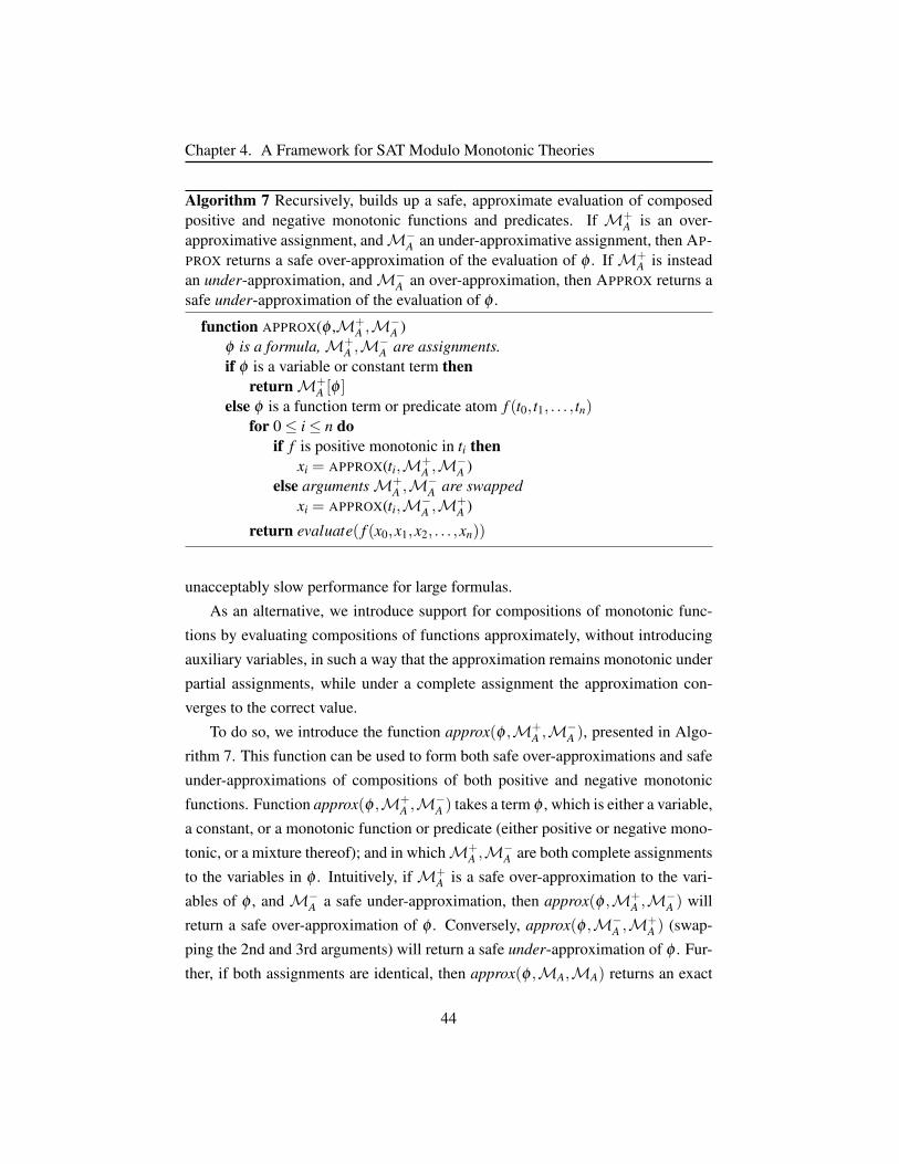
Chapter 4. A Framework for SAT Modulo Monotonic Theories
Algorithm 7 Recursively, builds up a safe, approximate evaluation of composedpositive and negative monotonic functions and predicates. If M+
A is an over-approximative assignment, andM−
A an under-approximative assignment, then AP-PROX returns a safe over-approximation of the evaluation of φ . IfM+
A is insteadan under-approximation, andM−
A an over-approximation, then APPROX returns asafe under-approximation of the evaluation of φ .
function APPROX(φ ,M+A ,M
−A )
φ is a formula,M+A ,M
−A are assignments.
if φ is a variable or constant term thenreturnM+
A [φ ]else φ is a function term or predicate atom f (t0, t1, . . . , tn)
for 0≤ i≤ n doif f is positive monotonic in ti then
xi = APPROX(ti,M+A ,M
−A )
else argumentsM+A ,M
−A are swapped
xi = APPROX(ti,M−A ,M
+A )
return evaluate( f (x0,x1,x2, . . . ,xn))
unacceptably slow performance for large formulas.
As an alternative, we introduce support for compositions of monotonic func-
tions by evaluating compositions of functions approximately, without introducing
auxiliary variables, in such a way that the approximation remains monotonic under
partial assignments, while under a complete assignment the approximation con-
verges to the correct value.
To do so, we introduce the function approx(φ ,M+A ,M
−A ), presented in Algo-
rithm 7. This function can be used to form both safe over-approximations and safe
under-approximations of compositions of both positive and negative monotonic
functions. Function approx(φ ,M+A ,M
−A ) takes a term φ , which is either a variable,
a constant, or a monotonic function or predicate (either positive or negative mono-
tonic, or a mixture thereof); and in whichM+A ,M
−A are both complete assignments
to the variables in φ . Intuitively, ifM+A is a safe over-approximation to the vari-
ables of φ , and M−A a safe under-approximation, then approx(φ ,M+
A ,M−A ) will
return a safe over-approximation of φ . Conversely, approx(φ ,M−A ,M
+A ) (swap-
ping the 2nd and 3rd arguments) will return a safe under-approximation of φ . Fur-
ther, if both assignments are identical, then approx(φ ,MA,MA) returns an exact
44

Chapter 4. A Framework for SAT Modulo Monotonic Theories
Algorithm 8 Replacement for PropagateBounds section of Algorithm 3. Sup-porting compositions of mixed positive and negative monotonic predicates andfunctions.
function PROPAGATEBOUNDS(M,M+A ,M
−A )
M,M+A ,M
−A are assignments, withM+
A ,M−A computed by UpdateBounds.
for each monotonic predicate atom p(t0, t1, . . .) doif ¬p ∈M then
if APPROX(p,M−A ,M
+A ) 7→ TRUE then
return FALSE,T-Analyze(M)else
Tighten bounds (optional)M← TIGHTENBOUNDS(p,M,M+
A ,M−A )
else if p ∈M thenif APPROX(p,M+
A ,M−A ) 7→ FALSE then
return FALSE,T-Analyze(M)else
Tighten bounds (optional)M← TIGHTENBOUNDS(¬p,M,M−
A ,M+A )
elseif APPROX(p,M−
A ,M+A ) 7→ TRUE then
M←M∪pelse if APPROX(p,M+
A ,M−A ) 7→ FALSE then
M←M∪¬preturn TRUE,M
evaluation of φ inMA.
Formally, if we have someM∗A such that ∀x,M+
A [x] ≥M∗A[x] ≥M
−A [x], then
approx(φ ,M+A ,M
−A )≥M∗
A[φ ]≥ approx(φ ,M−A ,M
+A ). A proof can be found in
Appendix C.2.
As approx(φ ,M+A ,M
−A ) and approx(φ ,M−
A ,M+A ) form safe, monotonic,
upper- and lower-bounds on the evaluation of MA[φ ], we can directly substitute
approx into Algorithm 3 in order to support compositions of mixed positive and
negative monotonic functions and predicates. These changes are described in Al-
gorithm 8.
In Algorithm 9, we introduce corresponding changes to the conflict set gener-
ation algorithm in order to support Algorithm 8. Algorithm 9 makes repeated calls
45

Chapter 4. A Framework for SAT Modulo Monotonic Theories
Algorithm 9 Conflict set generation for finite monotonic theories with functions.Allowing mixed positive and negative monotonic predicates and functions.
function T-Analyze(M)M is a partial assignment.ComputeM−
A ,M+A as in UpdateBounds.
for each Variable x of sort σ docase x < σ⊥ ∈M
return x < σ⊥case x > σ⊥ ∈M
return x > σ⊥case @σi : (σi ≥M−
A [x])∧ (σi ≤M+A [x])
return x≥M−A [x],x≤M
+A [x]
for each monotonic predicate atom p docase ¬p ∈M, APPROX(p,M−
A ,M+A ) 7→ TRUE
return ¬p∪ANALYZEAPPROX(p,≤,FALSE,M−A ,M
+A )
case p ∈M, APPROX(p,M+A ,M
−A ) 7→ FALSE
return p∪ANALYZEAPPROX(p,≥,TRUE,M+A ,M
−A )
to a recursive procedure, analyzeApprox (shown in Algorithm 10). Algorithm 10
produces a conflict set in terms of the upper and lower bounds of the variables x in
M+A andM−
A . Algorithm 10 recursively evaluates each predicate and function on
its respective upper and lower bounds, swapping the upper and lower bounds when
evaluating negatively monotonic arguments.
Notice that if p is positive monotonic, and ti is a ground variable, then Algo-
rithm 9 simply returns the same atom ti ≥ σi or ti ≤ σi, for some constant σi, as it
would in Algorithm 6. As such, Algorithm 9 directly generalizes Algorithm 6.
46
Chapter 4. A Framework for SAT Modulo Monotonic Theories
Algorithm 10 The analyzeApprox function provides conflict analysis for the re-cursive approx function.
function ANALYZEAPPROX(φ ,op,k,M+A ,M
−A )
φ is a formula, op is a comparison operator, k is a constant,M+A ,M
−A are
assignments.if φ is a constant term then
return else if φ is a variable then
if op is ≤ thenreturn φ ≤ k
elsereturn φ ≥ k
else φ is a function or predicate term f (t0, t1, . . . , tn)c←for 0≤ i≤ n do
if f is positive monotonic in ti thenxi = ANALYZEAPPROX(ti,M+
A ,M−A )
c← c∪ ANALYZEAPPROX(ti,op,xi,M+A ,M
−A )
else argumentsM+A ,M
−A are swapped
xi = ANALYZEAPPROX(ti,M−A ,M
+A )
c← c∪ ANALYZEAPPROX(ti,−op,xi,M−A ,M
+A )
return c
47
Chapter 4. A Framework for SAT Modulo Monotonic Theories
4.4 Monotonic Theories of Partially Ordered SortsAlgorithms 3 and 8, as presented above, assume finite, totally ordered sorts. How-
ever, observing that Lemma 4.1.1 applies also to partial-orders, Algorithms 3 and
8 can also be modified to handle finite, partially-ordered sorts.
Conceptually, theory propagation applied to partial orders proceeds similarly
to theory propagation as applied to total orders, with two major changes. Firstly,
checking whether the comparison atoms inM are consistent is slightly more in-
volved (and, correspondingly, conflict analysis for the case where the comparison
atoms are inconsistent is also more involved). Secondly, even in cases where the
comparison atoms are consistent, in a partial order there may not exist a constant
x+ to form the upper bound for variable x (or there may not exist a lower bound x−);
or those bounds may exist, but be very ‘loose’, and hence the theory propagation
procedure may fail to make deductions that are in fact implied by the comparison
atoms ofM.
For example, if σ is partially ordered, ¬(x ≥ y) does not necessarily imply
x < y, as it may also be possible for x and y to be assigned incomparable values;
consequently, it may be possible for both atoms ¬(x ≥ y),¬(x ≤ y) to be inMA
without implying a conflict. This causes complications for conflict analysis, and
also for the forming of upper and lower bounds needed by Algorithms 3 and 8.
In Algorithm 11, we describe modifications to the UpdateBounds section of
Algorithm 3 to support partially ordered sorts, by forming conservative lower and
upper bounds x− and x+, where possible, and returning without making deduc-
tions when such bounds do not exist. These changes are also compatible with the
changes to PropagateBounds described in Algorithm 8, and by combining both,
one can support theory propagation for finite monotonic theories with functions
and partially ordered sorts.
Unfortunately, if σ is only a partial order, then it is possible that either or both
of meet(max(X−)), join(min(X+)) may not exist. In the case that either or both do
not exist, Algorithm 11 simply returns, making no deductions at all. Consequently,
for partial orders, Algorithm 11 may fail to make deductions that are in fact implied
by the comparisons of MA (here, we define MA as we did in previous sections:
MA is a subset ofM containing assignments only to atoms comparing variables
48
Chapter 4. A Framework for SAT Modulo Monotonic Theories
to constants ((x ≤ σi), (x ≥ σi)). In fact, even in the case where safe upper and
lower bounds do exist, there may exist deductionsMA =⇒T
p (orMA =⇒T¬p)
that this algorithm fails to discover. In the special case that σ is totally ordered,
X+ and X− can always be represented as singletons (or the empty set, if there is
a conflict), max(X−) and min(X+) will always return single constants, the meet
and join will always be defined, and the resulting construction of x+,x− becomes
completely equivalent to our presentation in Algorithm 3.
The imprecision of Algorithm 11’s deductions is a consequence of reducing the
upper and lower bounds to singletons, which allows the upper and lower bounds of
each predicate p to be checked with only two evaluations of p (one for the upper
bound, and one for the lower bound). An alternative approach, which would dis-
cover all deductions MA =⇒T
p (or MA =⇒T¬p), would be to search over the
space of (incomparable) maximal and minimal elements max(x+) and min(x−) for
each variable x. In principle, by evaluating all possible combinations of maximal
and minimal assignments to each argument of p, one could find the absolute maxi-
mum and minimum evaluations of p. However, while there are general techniques
for optimizing functions over posets (see ordinal optimization, e.g. [78]), imple-
menting such a search would likely be impractical unless the domain of σ is very
small.
Above, we described a general purpose approach to handling monotonic theo-
ries over finite-domain partially ordered sorts. An alternative approach to support-
ing finite partially ordered sorts would be to convert the partial order into a total
order (e.g., using a topological sorting procedure), after which one could directly
apply the approach of Section 4.1. Unfortunately, strengthening the order relation-
ship between elements of the sort may force the solver to learn weaker clauses than
it otherwise would. For example, if a ≤ b holds in the total order, then Algorithm
6 may in some cases include that (spurious) comparison atom in learned clauses,
even if a and b are in fact incomparable in the original partial order.
An important special case of a partially ordered sort is a finite powerset lattice.
If the sort is a powerset lattice, then we can translate the space of possible subsets
into a bit string of Boolean variables, with each Boolean determining the presence
of each possible element in the set. In this case, the size of the represented set is
monotonic with respect to not only the value of the bit string, but also with respect
49
Chapter 4. A Framework for SAT Modulo Monotonic Theories
to each individual Boolean making up that string. This transformation allows one
to model the powerset lattice as a totally ordered, monotonic theory over the indi-
vidual Booleans of the bit string, and hence to perform theory propagation using
Algorithms 3 or 8. This is the approach that we take in our implementation of the
graph and finite state machine theories in Chapters 5 and 8, which operate over
sets of graphs and Kripke structures, respectively. We have found it to perform
very well in practice.
50

Chapter 4. A Framework for SAT Modulo Monotonic Theories
Algorithm 11 Replacement for UpdateBounds section of Algorithm 3, supportingtheory propagation for finite monotonic theories over partially ordered sorts.
function UPDATEBOUNDS(M)M−
A ←,M+A ←
for each variable x of sort σ doX+←σ⊥,σ1,σ2 . . .σ>X−←σ⊥,σ1,σ2 . . .σ>for each (x > σ j) inM do
X− = X− \∀σi|σi ≤ σ jfor each (x≥ σ j) inM do
X− = X− \∀σi|σi < σ jfor each ¬(x < σ j) inM do
X− = X− \∀σi|σi < σ jfor each ¬(x≤ σ j) inM do
X− = X− \∀σi|σi ≤ σ jfor each (x < σ j) inM do
X+ = X+ \∀σi|σi ≥ σ jfor each (x≤ σ j) inM do
X+ = X+ \∀σi|σi > σ jfor each ¬(x > σ j) inM do
X+ = X+ \∀σi|σi > σ jfor each ¬(x≥ σ j) inM do
X+ = X+ \∀σi|σi ≥ σ jif X+∩X− = then return FALSE,T-Analyze(M)
Note: As the minimal (resp. maximal) elements of X− (resp. X+) may notbe unique, min (resp. max) returns a set of minimal (resp. maximal) elements.
x−← meet(min(X−))x+← join(max(X+))if x− or x+ does not exist, or x− and x+ are incomparable then
return TRUE,Mif x− > x+ then return FALSE,T-Analyze(M)
M−A ←M
−A ∪(x≤ x−),(x≥ x−)
M+A ←M
+A ∪(x≤ x+),(x≥ x+)
51
Chapter 4. A Framework for SAT Modulo Monotonic Theories
4.5 Theory Combination and Infinite DomainsTwo additional concerns should be touched upon before continuing, both related to
the finite domain requirement of finite monotonic theories. First, we can ask, why
are the techniques introduced in this section restricted to finite domain sorts?
If the domain is infinite, then in the general case the conflict analysis proce-
dure (Algorithm 6 or Algorithm 9) may not be sufficient to guarantee termination,
as it may introduce a non-converging sequence of new comparison atoms with in-
finitesimally tighter bounds. Unfortunately, we have found no obvious way — in
the general case — to extend support to monotonic theories of infinite domains that
would resolve this concern.
The second concern is theory combination. In general, finite domain sorts —
including Booleans, bit vectors, and finite sets — violate the stably-infinite re-
quirement of Nelson-Oppen [156] theory combination, which requires that a the-
ory have, for every sort, an infinite number of satisfying assignments (models). As
such, Nelson-Oppen theory combination is not directly applicable to finite mono-
tonic theories.9
Finite domain theories can, in general, be combined at the propositional level
by introducing fresh variables for each shared variable in the two theories, and
then asserting equality at the propositional level. This can either be accomplished
by passing equality predicates over shared constants between the two theories (as in
Nelson-Oppen), or by enumerating over the space of possible values each variable
can take and asserting that exactly the same assignment is chosen for those fresh
variables.
Either of the above theory combination approaches are poor choices for mono-
tonic theories, for the reason that it provides a very poor mechanism for communi-
cating derived bounds on the satisfiable ranges of each variable between each the-
ory solver, when operating on partial assignments. For example, when operating
on a partial assignment, one theory solver may have derived the bounds 3≤ x≤ 5,
9Note that, even if we were to consider monotonic theories with infinite domains, we would stillencounter a difficulty, which is that the theory of equality is non-monotonic, and hence monotonictheories do not directly support equality predicates. It seems hopeful that Nelson-Oppen style theorycombination could be applied to theories supporting only comparisons, for example by emulatingequality through conjunctions of ≤,≥ constraints. However, we present no proof of this claim.
52
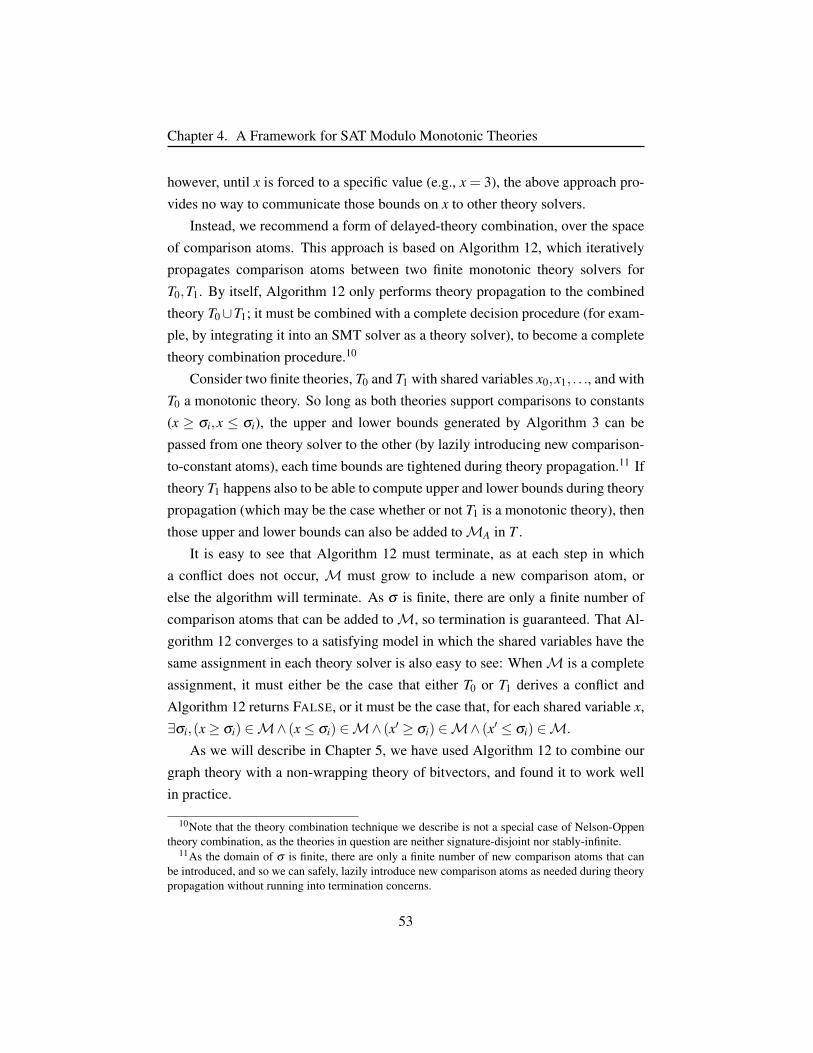
Chapter 4. A Framework for SAT Modulo Monotonic Theories
however, until x is forced to a specific value (e.g., x = 3), the above approach pro-
vides no way to communicate those bounds on x to other theory solvers.
Instead, we recommend a form of delayed-theory combination, over the space
of comparison atoms. This approach is based on Algorithm 12, which iteratively
propagates comparison atoms between two finite monotonic theory solvers for
T0,T1. By itself, Algorithm 12 only performs theory propagation to the combined
theory T0∪T1; it must be combined with a complete decision procedure (for exam-
ple, by integrating it into an SMT solver as a theory solver), to become a complete
theory combination procedure.10
Consider two finite theories, T0 and T1 with shared variables x0,x1, . . ., and with
T0 a monotonic theory. So long as both theories support comparisons to constants
(x ≥ σi,x ≤ σi), the upper and lower bounds generated by Algorithm 3 can be
passed from one theory solver to the other (by lazily introducing new comparison-
to-constant atoms), each time bounds are tightened during theory propagation.11 If
theory T1 happens also to be able to compute upper and lower bounds during theory
propagation (which may be the case whether or not T1 is a monotonic theory), then
those upper and lower bounds can also be added toMA in T .
It is easy to see that Algorithm 12 must terminate, as at each step in which
a conflict does not occur, M must grow to include a new comparison atom, or
else the algorithm will terminate. As σ is finite, there are only a finite number of
comparison atoms that can be added toM, so termination is guaranteed. That Al-
gorithm 12 converges to a satisfying model in which the shared variables have the
same assignment in each theory solver is also easy to see: WhenM is a complete
assignment, it must either be the case that either T0 or T1 derives a conflict and
Algorithm 12 returns FALSE, or it must be the case that, for each shared variable x,
∃σi,(x≥ σi) ∈M∧ (x≤ σi) ∈M∧ (x′ ≥ σi) ∈M∧ (x′ ≤ σi) ∈M.
As we will describe in Chapter 5, we have used Algorithm 12 to combine our
graph theory with a non-wrapping theory of bitvectors, and found it to work well
in practice.
10Note that the theory combination technique we describe is not a special case of Nelson-Oppentheory combination, as the theories in question are neither signature-disjoint nor stably-infinite.
11As the domain of σ is finite, there are only a finite number of new comparison atoms that canbe introduced, and so we can safely, lazily introduce new comparison atoms as needed during theorypropagation without running into termination concerns.
53
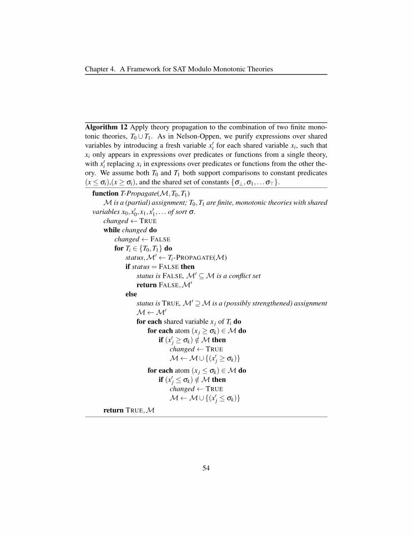
Chapter 4. A Framework for SAT Modulo Monotonic Theories
Algorithm 12 Apply theory propagation to the combination of two finite mono-tonic theories, T0 ∪ T1. As in Nelson-Oppen, we purify expressions over sharedvariables by introducing a fresh variable x′i for each shared variable xi, such thatxi only appears in expressions over predicates or functions from a single theory,with x′i replacing xi in expressions over predicates or functions from the other the-ory. We assume both T0 and T1 both support comparisons to constant predicates(x≤ σi),(x≥ σi), and the shared set of constants σ⊥,σ1, . . .σ>.
function T-Propagate(M,T0,T1)M is a (partial) assignment; T0,T1 are finite, monotonic theories with shared
variables x0,x′0,x1,x′1, . . . of sort σ .changed← TRUE
while changed dochanged← FALSE
for Ti ∈ T0,T1 dostatus,M′← Ti-PROPAGATE(M)if status = FALSE then
status is FALSE,M′ ⊆M is a conflict setreturn FALSE,M′
elsestatus is TRUE,M′⊇M is a (possibly strengthened) assignmentM←M′
for each shared variable x j of Ti dofor each atom (x j ≥ σk) ∈M do
if (x′j ≥ σk) /∈M thenchanged← TRUE
M←M∪(x′j ≥ σk)for each atom (x j ≤ σk) ∈M do
if (x′j ≤ σk) /∈M thenchanged← TRUE
M←M∪(x′j ≤ σk)return TRUE,M
54

Chapter 5
Monotonic Theory of Graphs
Chapter 4 described a set of techniques for building lazy SMT solvers for finite,
monotonic theories. In this chapter, we introduce a set of monotonic graph pred-
icates collected into a theory of graphs, as well as an implementation of an SMT
solver for this theory, built using the SMMT framework.
Many well-known graph properties — such as reachability, shortest path,
acyclicity, maximum s-t flow, and minimum spanning tree weight — are mono-
tonic with respect to the edges or edge weights in a graph. We describe our support
for predicates over these graph properties in detail in Section 5.2.
The corresponding graph theory solver for these predicates forms the largest
part of our SMT solver, MONOSAT (described in Appendix A). In Section 5.1, we
give an overview of our implementation, using the techniques described in Chapter
4. In Section 5.3, we extend support to bitvector weighted edges, by combining the
theory of graphs with a theory of bitvectors.
In later chapters, we will describe how we have successfully applied this theory
of graphs to problems ranging from procedural content generation (Chapter 6.1) to
PCB layout (Chapter 6.2), in the latter case solving complex, real-world graph con-
straints with more than 1,000,000 nodes — a massive improvement in scalability
over comparable SAT-based techniques.
55
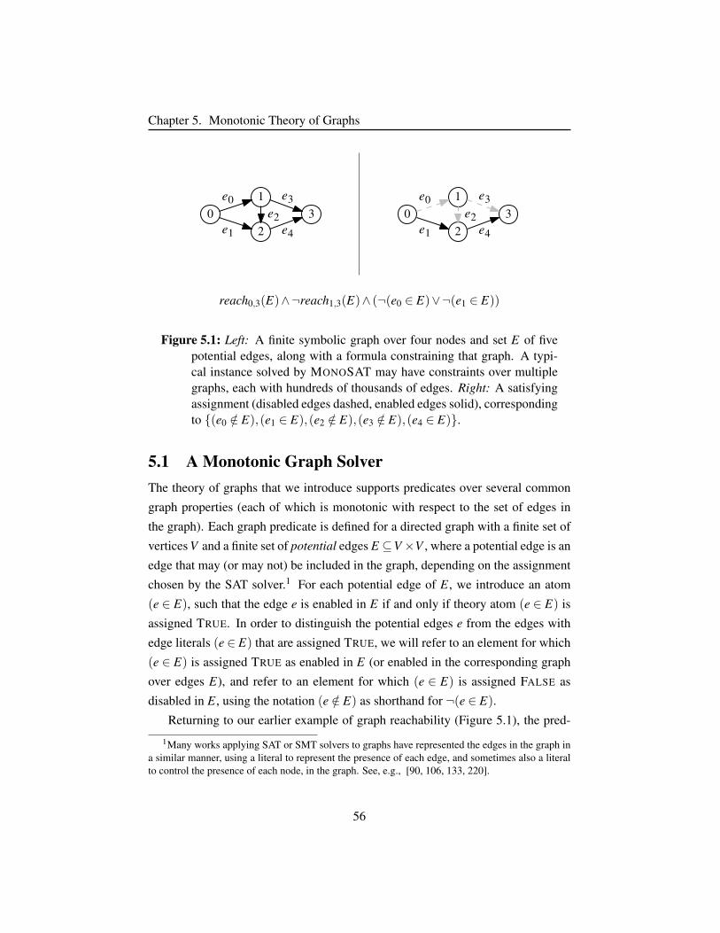
Chapter 5. Monotonic Theory of Graphs
01e0
2e1
e2 3e3
e4
01e0
2e1
e2 3e3
e4
reach0,3(E)∧¬reach1,3(E)∧ (¬(e0 ∈ E)∨¬(e1 ∈ E))
Figure 5.1: Left: A finite symbolic graph over four nodes and set E of fivepotential edges, along with a formula constraining that graph. A typi-cal instance solved by MONOSAT may have constraints over multiplegraphs, each with hundreds of thousands of edges. Right: A satisfyingassignment (disabled edges dashed, enabled edges solid), correspondingto (e0 /∈ E),(e1 ∈ E),(e2 /∈ E),(e3 /∈ E),(e4 ∈ E).
5.1 A Monotonic Graph SolverThe theory of graphs that we introduce supports predicates over several common
graph properties (each of which is monotonic with respect to the set of edges in
the graph). Each graph predicate is defined for a directed graph with a finite set of
vertices V and a finite set of potential edges E ⊆V×V , where a potential edge is an
edge that may (or may not) be included in the graph, depending on the assignment
chosen by the SAT solver.1 For each potential edge of E, we introduce an atom
(e ∈ E), such that the edge e is enabled in E if and only if theory atom (e ∈ E) is
assigned TRUE. In order to distinguish the potential edges e from the edges with
edge literals (e ∈ E) that are assigned TRUE, we will refer to an element for which
(e ∈ E) is assigned TRUE as enabled in E (or enabled in the corresponding graph
over edges E), and refer to an element for which (e ∈ E) is assigned FALSE as
disabled in E, using the notation (e /∈ E) as shorthand for ¬(e ∈ E).
Returning to our earlier example of graph reachability (Figure 5.1), the pred-
1Many works applying SAT or SMT solvers to graphs have represented the edges in the graph ina similar manner, using a literal to represent the presence of each edge, and sometimes also a literalto control the presence of each node, in the graph. See, e.g., [90, 106, 133, 220].
56
Chapter 5. Monotonic Theory of Graphs
icate reachs,t(E) is TRUE if and only if node t is reachable from node s in graph
G, under a given assignment to the edge literals (ei ∈ E). As previously observed,
given a graph (directed or undirected) and some fixed starting node s, enabling
an edge in E can increase the set of nodes that are reachable from s, but cannot
decrease the set of reachable nodes. The other graph predicates we consider are
each similarly positive or negative monotonic with respect to the set of edges in the
graph; for example, enabling an edge in a graph may decrease the weight of the
minimum spanning tree of that graph, but cannot increase it.
Theory propagation as implemented in our theory of graphs is described in Al-
gorithm 13, which closely follows Algorithm 3. Algorithm 13 representsM+A ,M
−A
in the form of two concrete graphs, G− and G+. The graph G− is formed from the
edge assignments in MA: only edges e for which the atom (e ∈ E) is in M are
included in G−. In the second graph, G+, we include all edges for which (e /∈ E)
is not inMA.
Algorithm 13 makes some minor improvements over Algorithm 3. The first is
that we re-use the data structures for G−,G+ across separate calls to T-Propagate,
updating them by adding or removing edges as necessary. As the graphs can be
very large (e.g., in Section 6.2 we will consider applications with hundreds of
thousands or even millions of edges), and there are typically only a few edges
either added or removed between calls to T-Propagate, this saves a large amount of
redundant effort that would otherwise be caused by repeatedly creating the graphs.
A second improvement is to check whether, under the current partial assign-
ment, either G− or G+ is unchanged from the previous call to T-Propagate. If the
solver has only enabled edges in E (resp. only disabled edges in E) since the last
theory propagation call, then the graph G+ (resp. G−) will not have changed, and
so we do not need to recompute properties for that graph.
Each time an assignment is made to a graph theory atom, Algorithm 13 eval-
uates each predicate atom on both the under- and over-approximative graphs G−
and G+. The practical performance of this scheme can be greatly improved by us-
ing partially or fully dynamic graph algorithms, which can be efficiently updated
as edges are removed or added to G− or G+. Similarly, care should be taken to
represent G− and G+ using data structures that can be cheaply updated as edges
are removed and added. In our implementation, we use an adjacency list in which
57

Chapter 5. Monotonic Theory of Graphs
Algorithm 13 Theory propagation for the theory of graphs, adapted from Algo-rithm 3. M is a (partial) assignment. E−,E+ are sets of edges; G−,G+ are under-and over-approximate graphs. T-Propagate returns a tuple (FALSE, conflict) ifMis found to be unsatisfiable, and returns tuple (TRUE,M) otherwise.
function T-Propagate(M)UpdateBounds:E−←,E+←Efor each finite symbolic graph G = (V,E) do
for each edge ei of E doif (ei /∈ E) ∈M then
E+← E+ \eiif (ei ∈ E) ∈M then
E−← E−∪eiG−← (V,E−),G+← (V,E+)
PropagateBounds:for each predicate atom p(E) do
If p is negative monotonic, swap G−,G+ below.if ¬p ∈M then
if evaluate(p,G−) thenreturn FALSE,analyze(p,G−)
else if p ∈M thenif not evaluate(p,G+) 7→ FALSE then
return FALSE,analyze(¬p,G+)
elseif evaluate(p,G−) thenM←M∪p
else if not evaluate(p,G+) thenM←M∪¬p
return TRUE,M
every possible edge of E has a unique integer ID. These IDs map to corresponding
edge literals (e ∈ E) and are useful for conflict analysis, in which we often must
work backwards from graph analyses to identify the theory literals correspond-
ing to a subset of relevant edges. Each adjacency list also maintains a history of
added/removed edges, which facilitates the use of dynamic graph algorithms in the
solver.
58

Chapter 5. Monotonic Theory of Graphs
5.2 Monotonic Graph PredicatesMany of the most commonly used properties of graphs are monotonic with respect
to the edges in the graph. A few well-known examples include:
1. Reachability
2. Acyclicity
3. Connected component count
4. Shortest s-t path
5. Maximum s-t flow
6. Minimum spanning tree weight
The first three properties are unweighted, while the remainder operate over
weighted graphs and are monotonic with respect to both the set of edges and the
weights of those edges. For example, the length of the shortest path from node s
to node t in a graph may increase as the length of an edge is increased, but cannot
decrease.
These are just a few examples of the many graph predicates that are monotonic
with respect to the edges in the graph; there are many others that are also monotonic
and which may be useful (a few examples: planarity testing/graph skew, graph
diameter, minimum global cut, minimum-cost maximum flow, and Hamiltonian-
circuit). Some examples of non-monotonic graph properties include Eulerian-
circuit (TRUE iff the graph has an Eulerian-circuit) and Graph-Isomorphism (TRUE
iff two graphs are isomorphic to each other).
For each predicate p in the theory solver we implement three functions:
1. evaluate(p,G), which takes a concrete graph (it may be the under-, or the
over-approximative graph) and returns TRUE iff p holds in the edges of G,
2. analyze(p,G), which takes a concrete graph G in which p evaluates to TRUE
and returns a justification set for p, and
3. analyze(¬p,G), which takes a concrete graph G in which p evaluates to
FALSE and returns a justification set for ¬p.
59

Chapter 5. Monotonic Theory of Graphs
Each of these functions is used by Algorithm 13 to implement theory propaga-
tion and conflict analysis. In Sections 5.2.1 and 5.2.2, we describe the implementa-
tion of our theory solvers for reachability and acyclicity predicates; subsequently,
in Section 5.3.1, we describe our implementation of a theory solver for maximum
s-t flow over weighted graphs. In Appendix D.1, we list our implementations of
the remaining supported graph properties mentioned above.
5.2.1 Graph Reachability
01e0
2e1
e2 3e3
e4
01e0,∞
2e1,1e2,1 3
e3,1
e4,∞
Figure 5.2: Left: A finite symbolic graph of edges E under assignment(e0 ∈ E),(e1 ∈ E),(e2 ∈ E),(e3 /∈ E),(e4 ∈ E) in which reach0,3(E)holds. Edges e1,e4 (bold) form a shortest-path from node 0 to node 3.Right: The same graph under the assignment (e0 ∈ E),(e1 /∈ E),(e2 /∈E),(e3 /∈ E),(e4 ∈ E), in which reach0,3(E) does not hold. A cut (red)of disabled edges e1,e2,e3 separates node 0 from node 3.
The first monotonic graph predicate we consider in detail is reachability in a finite
graph (from a fixed starting node to a fixed ending node). A summary of our
implementation can be found in Figure 5.3.
Both directed and undirected reachability constraints on explicit graphs arise
in many contexts in SAT solvers.2 A few applications of SAT solvers in which
2As with all the other graph predicates we consider here, this reachability predicate operates ongraphs represented in explicit form, for example, as an adjacency list or matrix. This is in contrastto safety properties as considered in model checking [35, 47, 58], which can be described as testingthe reachability of a node in a (vast) graph represented in an implicit form (i.e., as a BDD or SATformula). Although SAT solvers are commonly applied to implicit graph reachability tasks such asmodel checking and planning, the techniques we describe in this section are not appropriate for modelchecking implicitly represented state graphs; nor are techniques such as SAT-based bounded [35] orunbounded [41] model checking appropriate for the explicit graph synthesis problems we consider.
60
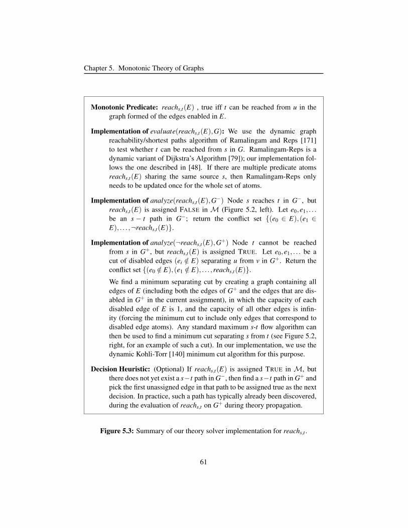
Chapter 5. Monotonic Theory of Graphs
Monotonic Predicate: reachs,t(E) , true iff t can be reached from u in thegraph formed of the edges enabled in E.
Implementation of evaluate(reachs,t(E),G): We use the dynamic graphreachability/shortest paths algorithm of Ramalingam and Reps [171]to test whether t can be reached from s in G. Ramalingam-Reps is adynamic variant of Dijkstra’s Algorithm [79]); our implementation fol-lows the one described in [48]. If there are multiple predicate atomsreachs,t(E) sharing the same source s, then Ramalingam-Reps onlyneeds to be updated once for the whole set of atoms.
Implementation of analyze(reachs,t(E),G−) Node s reaches t in G−, butreachs,t(E) is assigned FALSE in M (Figure 5.2, left). Let e0,e1, . . .be an s − t path in G−; return the conflict set (e0 ∈ E),(e1 ∈E), . . . ,¬reachs,t(E).
Implementation of analyze(¬reachs,t(E),G+) Node t cannot be reachedfrom s in G+, but reachs,t(E) is assigned TRUE. Let e0,e1, . . . be acut of disabled edges (ei /∈ E) separating u from v in G+. Return theconflict set (e0 /∈ E),(e1 /∈ E), . . . ,reachs,t(E).We find a minimum separating cut by creating a graph containing alledges of E (including both the edges of G+ and the edges that are dis-abled in G+ in the current assignment), in which the capacity of eachdisabled edge of E is 1, and the capacity of all other edges is infin-ity (forcing the minimum cut to include only edges that correspond todisabled edge atoms). Any standard maximum s-t flow algorithm canthen be used to find a minimum cut separating s from t (see Figure 5.2,right, for an example of such a cut). In our implementation, we use thedynamic Kohli-Torr [140] minimum cut algorithm for this purpose.
Decision Heuristic: (Optional) If reachs,t(E) is assigned TRUE in M, butthere does not yet exist a s−t path in G−, then find a s−t path in G+ andpick the first unassigned edge in that path to be assigned true as the nextdecision. In practice, such a path has typically already been discovered,during the evaluation of reachs,t on G+ during theory propagation.
Figure 5.3: Summary of our theory solver implementation for reachs,t .
61
Chapter 5. Monotonic Theory of Graphs
reachability constraints play an integral role include many variations of routing
problems (e.g., FPGA and PCB routing [153, 154, 177, 203] and optical switch
routing [5, 102]), Hamiltonian cycle constraints [133, 220], and product line con-
figuration [6, 149, 150]. The SAT-based solver for the Alloy relational modeling
language[130] encodes transitive closure into CNF as a reachability constraint over
an explicit graph [129, 131].
There are several common ways to encode reachability constraints into SAT
and SMT solvers described in the literature. Some works encode reachability di-
rectly into CNF by what amounts to unrolling the Floyd-Warshall algorithm sym-
bolically (e.g., [177]); unfortunately, this approach requires O(|E| · |V |2) clauses
and hence scales very poorly.
SMT solvers have long had efficient, dedicated support for computing congru-
ence closure over equality relations[19, 157, 159, 160], which amounts to fast all-
pairs undirected reachability detection.3 Undirected reachability constraints can be
encoded into equality constraints (by introducing a fresh variable for each vertex,
and an equality constraint between neighbouring vertices that is enforced only if
an arc between neighbouring vertices is enabled). The resulting encoding is ef-
ficient and requires only O(|V |+ |E|) constraints, however, the encoding is only
one-sided: it can enforce that two nodes must not be connected, but it cannot en-
force that they must be connected. Further, this equality constraint encoding cannot
enforce directed reachability constraints at all.
While equality constraints cannot encode directed reachability, directed reach-
ability constraints can still be encoded into SMT solvers using arithmetic theories.
An example of such an approach is described in [90]. This approach introduces a
non-deterministic distance variable for each node other than source (which is set to
a distance of zero), and then adds constraints for every node other than the source
node, enforcing that each node’s distance is one greater than its nearest-to-source
neighbor, or is set to some suitably large constant if none of its neighbours are
reachable from source. This approach requires O(|E| · |V | · log |V |) constraints if
distances are encoded in bit-blasted bitvectors, or O(|E| · |V |) constraints if dis-
We will consider applications related to model checking in Chapter 8.3Note: Some writers distinguish undirected reachability from directed reachability using the term
connectivity for the undirected variant.
62
Chapter 5. Monotonic Theory of Graphs
tances are instead encoded in linear or integer arithmetic. However, while this
produces a concise encoding, it forces the solver to non-deterministically guess the
distance to each node, which in practice seems to work very poorly (see Figure
5.4). 4
In addition to SAT and SMT solvers, many works have recently used answer
set programming (ASP) [25] constraint solvers to enforce reachability constraints.
Modern ASP solvers are closely related to CDCL solvers, however, unlike SAT,
ASP can encode reachability constraints on arbitrary directed graphs in linear
space, and ASP solvers can solve the resulting formulas efficiently in practice.
The ASP solver CLASP [104], which is implemented as an extended CDCL solver,
has been particularly widely used to enforce reachability constraints for procedu-
ral content generation applications (e.g. [125, 182, 183, 219] all apply CLASP to
procedural content generation using reachability constraints).
Considered on its own, the directed reachability predicate implemented in
MONOSAT’s theory of graphs scales dramatically better than any of the above
approaches for directed reachability, as can be seen in Figure 5.4.5 In Section 6.1,
we will see that this translates into real performance improvements in cases where
the constraints are dominated by a small number of reachability predicates. How-
ever, in cases where a large number of reachability predicates are used (and in
particular, in cases where those reachability predicates are mutually unsatisfiable
or nearly unsatisfiable), this approach to reachability predicates scales poorly.
4If only one-sided directed reachability constraints are required (i.e., the formula is satisfiableonly if node s reaches node t), then more efficient encodings are possible, by having the SAT solvernon-deterministically guess a path. Some examples of one-sided reachability encodings are describedin [106].
5All experiments in this chapter were run on a 2.67GHz Intel x5650 CPU (12Mb L3, 96 GbRAM), on Ubuntu 12.04, restricted to 10,000 seconds of CPU time, and 16 GB of RAM.
63
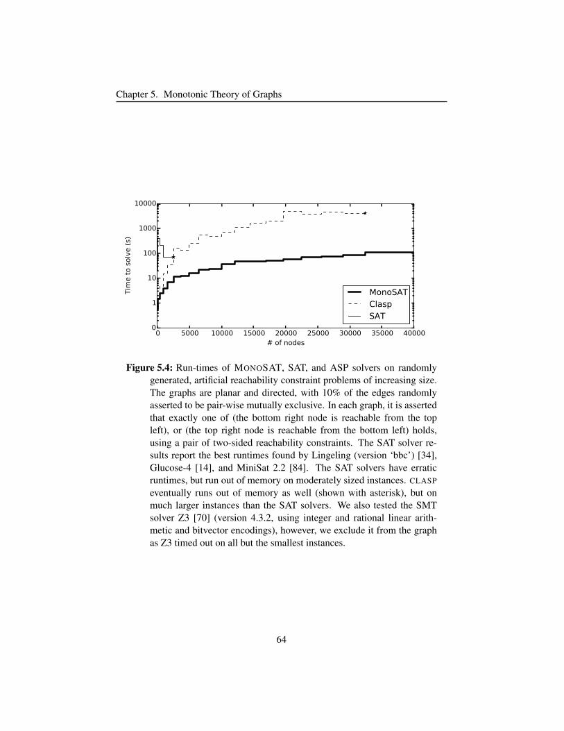
Chapter 5. Monotonic Theory of Graphs
0 5000 10000 15000 20000 25000 30000 35000 40000# of nodes
0
1
10
100
1000
10000
Tim
e to
sol
ve (s
)
MonoSATClaspSAT
Figure 5.4: Run-times of MONOSAT, SAT, and ASP solvers on randomlygenerated, artificial reachability constraint problems of increasing size.The graphs are planar and directed, with 10% of the edges randomlyasserted to be pair-wise mutually exclusive. In each graph, it is assertedthat exactly one of (the bottom right node is reachable from the topleft), or (the top right node is reachable from the bottom left) holds,using a pair of two-sided reachability constraints. The SAT solver re-sults report the best runtimes found by Lingeling (version ‘bbc’) [34],Glucose-4 [14], and MiniSat 2.2 [84]. The SAT solvers have erraticruntimes, but run out of memory on moderately sized instances. CLASP
eventually runs out of memory as well (shown with asterisk), but onmuch larger instances than the SAT solvers. We also tested the SMTsolver Z3 [70] (version 4.3.2, using integer and rational linear arith-metic and bitvector encodings), however, we exclude it from the graphas Z3 timed out on all but the smallest instances.
64
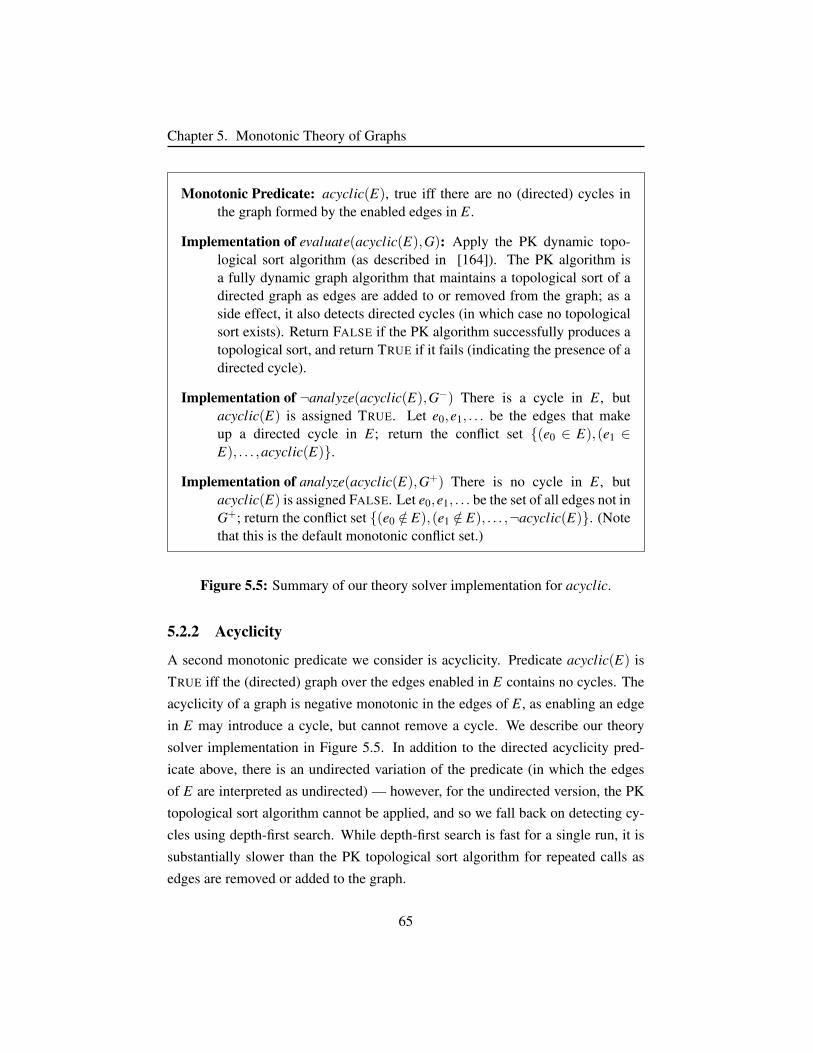
Chapter 5. Monotonic Theory of Graphs
Monotonic Predicate: acyclic(E), true iff there are no (directed) cycles inthe graph formed by the enabled edges in E.
Implementation of evaluate(acyclic(E),G): Apply the PK dynamic topo-logical sort algorithm (as described in [164]). The PK algorithm isa fully dynamic graph algorithm that maintains a topological sort of adirected graph as edges are added to or removed from the graph; as aside effect, it also detects directed cycles (in which case no topologicalsort exists). Return FALSE if the PK algorithm successfully produces atopological sort, and return TRUE if it fails (indicating the presence of adirected cycle).
Implementation of ¬analyze(acyclic(E),G−) There is a cycle in E, butacyclic(E) is assigned TRUE. Let e0,e1, . . . be the edges that makeup a directed cycle in E; return the conflict set (e0 ∈ E),(e1 ∈E), . . . ,acyclic(E).
Implementation of analyze(acyclic(E),G+) There is no cycle in E, butacyclic(E) is assigned FALSE. Let e0,e1, . . . be the set of all edges not inG+; return the conflict set (e0 /∈ E),(e1 /∈ E), . . . ,¬acyclic(E). (Notethat this is the default monotonic conflict set.)
Figure 5.5: Summary of our theory solver implementation for acyclic.
5.2.2 Acyclicity
A second monotonic predicate we consider is acyclicity. Predicate acyclic(E) is
TRUE iff the (directed) graph over the edges enabled in E contains no cycles. The
acyclicity of a graph is negative monotonic in the edges of E, as enabling an edge
in E may introduce a cycle, but cannot remove a cycle. We describe our theory
solver implementation in Figure 5.5. In addition to the directed acyclicity pred-
icate above, there is an undirected variation of the predicate (in which the edges
of E are interpreted as undirected) — however, for the undirected version, the PK
topological sort algorithm cannot be applied, and so we fall back on detecting cy-
cles using depth-first search. While depth-first search is fast for a single run, it is
substantially slower than the PK topological sort algorithm for repeated calls as
edges are removed or added to the graph.
65
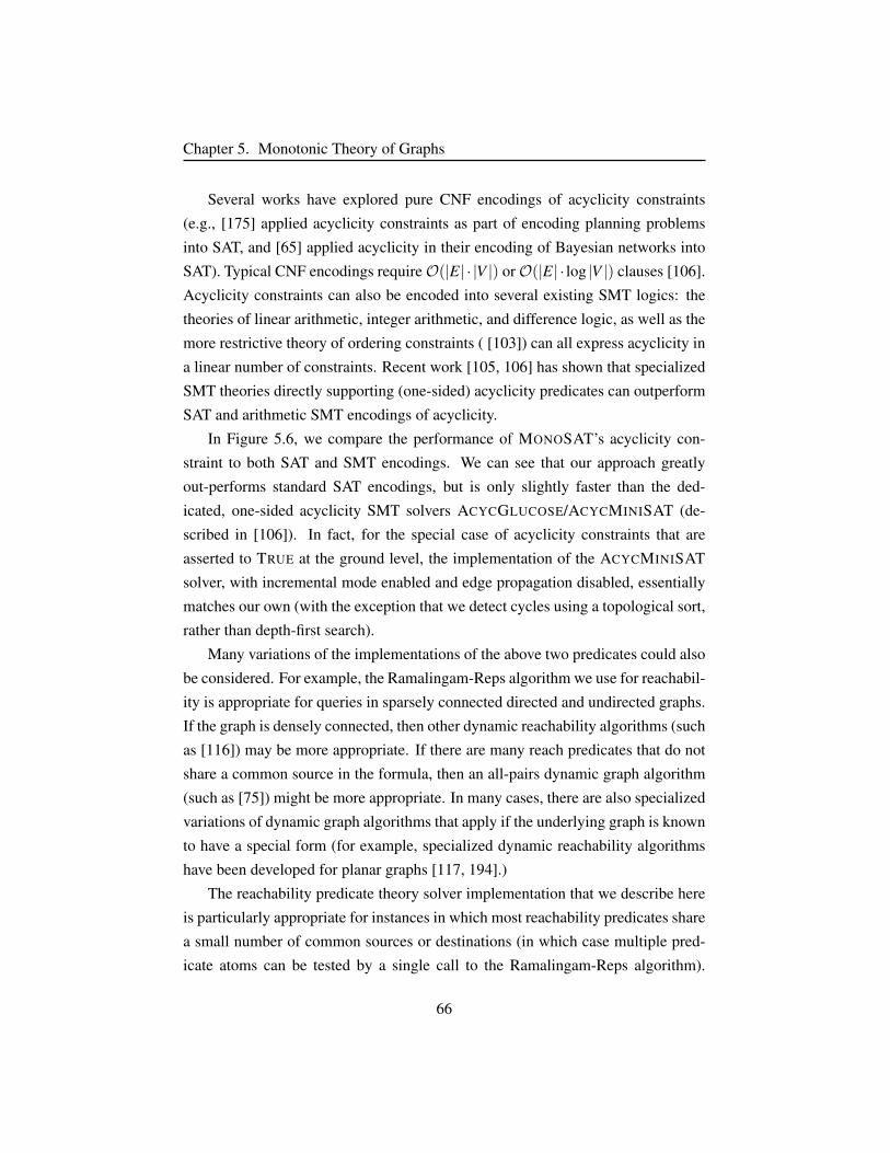
Chapter 5. Monotonic Theory of Graphs
Several works have explored pure CNF encodings of acyclicity constraints
(e.g., [175] applied acyclicity constraints as part of encoding planning problems
into SAT, and [65] applied acyclicity in their encoding of Bayesian networks into
SAT). Typical CNF encodings requireO(|E| · |V |) orO(|E| · log |V |) clauses [106].
Acyclicity constraints can also be encoded into several existing SMT logics: the
theories of linear arithmetic, integer arithmetic, and difference logic, as well as the
more restrictive theory of ordering constraints ( [103]) can all express acyclicity in
a linear number of constraints. Recent work [105, 106] has shown that specialized
SMT theories directly supporting (one-sided) acyclicity predicates can outperform
SAT and arithmetic SMT encodings of acyclicity.
In Figure 5.6, we compare the performance of MONOSAT’s acyclicity con-
straint to both SAT and SMT encodings. We can see that our approach greatly
out-performs standard SAT encodings, but is only slightly faster than the ded-
icated, one-sided acyclicity SMT solvers ACYCGLUCOSE/ACYCMINISAT (de-
scribed in [106]). In fact, for the special case of acyclicity constraints that are
asserted to TRUE at the ground level, the implementation of the ACYCMINISAT
solver, with incremental mode enabled and edge propagation disabled, essentially
matches our own (with the exception that we detect cycles using a topological sort,
rather than depth-first search).
Many variations of the implementations of the above two predicates could also
be considered. For example, the Ramalingam-Reps algorithm we use for reachabil-
ity is appropriate for queries in sparsely connected directed and undirected graphs.
If the graph is densely connected, then other dynamic reachability algorithms (such
as [116]) may be more appropriate. If there are many reach predicates that do not
share a common source in the formula, then an all-pairs dynamic graph algorithm
(such as [75]) might be more appropriate. In many cases, there are also specialized
variations of dynamic graph algorithms that apply if the underlying graph is known
to have a special form (for example, specialized dynamic reachability algorithms
have been developed for planar graphs [117, 194].)
The reachability predicate theory solver implementation that we describe here
is particularly appropriate for instances in which most reachability predicates share
a small number of common sources or destinations (in which case multiple pred-
icate atoms can be tested by a single call to the Ramalingam-Reps algorithm).
66
Chapter 5. Monotonic Theory of Graphs
0 5000 10000 15000 20000 25000 30000 35000# of nodes
0
0
0
1
10
100
1000
10000Ti
me
to s
olve
(s)
MonoSATAcycglucoseSAT
Figure 5.6: Run-times of SAT and SMT solvers on randomly generated, ar-tificial acyclicity constraint problems of increasing size. We considergrids of edges, constrained to be partitioned into two graphs such thatboth graphs are disjoint and acyclic. The graphs are planar and directed,with 0.1% of the edges randomly asserted to be pair-wise mutually ex-clusive. The plain SAT entry represents the best runtimes obtained bythe solvers Lingeling (version ‘bbc’) [34], Glucose-4 [14], or MiniSat2.2 [84]. The SAT solvers run out of memory at 5000 edges, so wedo not report results for SAT for larger instances. The ACYCGLUCOSE
entry represents the best runtimes for ACYCGLUCOSE and ACYCMIN-ISAT, with and without pre-processing, incremental mode, and edgepropagation. While both MONOSAT and ACYCGLUCOSE greatly out-perform a plain CNF encoding, the runtimes of MONOSAT and ACY-CGLUCOSE are comparable (with MONOSAT having a slight edge).
Two recent works [90, 152] introduced SMT solvers designed for VLSI and clock
routing (both of which entail solving formulas with many reachability or shortest
path predicates with distinct sources and destinations). In [152] the authors pro-
vide an experimental comparison against our graph theory solver (as implemented
in MONOSAT), demonstrating that their approach scales substantially better than
ours for VLSI and clock routing problems. In the future, it may be possible to in-
tegrate the sophisticated decision heuristics described in those works into MONO-
SAT. In Section 6.2, we also describe a third type of routing problem, escape
routing, for which we obtain state-of-the-art performance using the maximum flow
predicate support that we discuss in the next section.
67
Chapter 5. Monotonic Theory of Graphs
5.3 Weighted Graphs & BitvectorsIn Section 5.2, we considered two predicates that take a single argument (the set
of edges, E), operating on an unweighted, directed graph. These two predicates,
reachability and acyclicity, have many applications ranging from procedural con-
tent generation to circuit layout (for example, in a typical circuit layout application,
one must connect several positions in a graph, while ensuring that the wires are
acyclic and non-crossing).
However, many common graph properties, such as maximum s-t flow, shortest
s-t path, or minimum spanning tree weight, are more naturally posed as comparison
predicates operating over graphs with variable edge weights (or edge capacities).6
As described in Section 4.5, a monotonic theory over a finite sort σ can be com-
bined with another theory over σ , so long as that other theory supports comparison
operators, with the two theory solvers communicating only through exchanges of
atoms comparing variables to constants: (x ≤ c),(x < c). Extending Algorithm
13 to support bitvector arguments in this way requires only minor changes to the-
ory propagation in the graph solver (shown in Algorithm 14); it also requires us
to introduce a bitvector theory solver capable of efficiently deriving tight compari-
son atoms over its bitvector arguments. We describe our bitvector theory solver in
Appendix B.
5.3.1 Maximum Flow
The maximum s-t flow in a weighted, directed graph, in which each edge of E has
an associated capacity c, is positive monotonic with respect to both the set of edges
enabled in E, and also with respect to the capacity of each edge. We introduce
a predicate maxFlows,tE,m,c0,c1, . . ., with E a set of edges, and m,c0,c1, . . . fixed
width bit-vectors, which evaluates to TRUE iff the maximum s-t flow in the directed
graph induced by edges E, with edge capacities c0,c1, . . ., is greater or equal to m.7
6It is also possible to consider these predicates over constant edge-weight graphs. We describedsuch an approach in [33]; one can recover that formulation from our presentation here by simplysetting each bitvector variable to a constant value.
7There is also a variation of this predicate supporting strictly greater than comparisons, but wedescribe only the ‘greater or equal to’ variant. It is also possible to describe this predicate insteadas a function that returns the maximum flow, constrained by a bitvector comparison constraint. Fortechnical reasons this function-oriented presentation is less convenient in our implementation.
68

Chapter 5. Monotonic Theory of Graphs
01e0,1/2
2e1,1/2
e2,1/1 3
e3,0/3
e4,2/20
1
23∞∞ 1 1
2
1
1
1
0
1
Figure 5.7: Left: Over-approximate graph G+ for the partial assignment(e1 ∈ E),(e2 ∈ E),(e3 /∈ E),(e4 ∈ E), with (e0 ∈ E) unassigned. Themaximum 0-3 flow in this graph is 2; each edge has its assigned flowand capacity shown as f/c. Right: The cut graph Gcut for this assign-ment, with corresponding minimum 0-3 cut (red): e3,e4. Either edgee3 must be included in the graph, or the capacity of edge e4 must beincreased, in order for the maximum flow to be greater than 2.
This predicate is positive monotonic with respect to the edge literals and their
capacity bitvectors: Enabling an edge in E can increase but cannot decrease the
maximum flow; increasing the capacity of an edge can increase but cannot decrease
the maximum flow. It is negative monotonic with respect to the flow comparison
bitvector m. We summarize our theory solver implementation in Figure 5.8.
Maximum flow constraints appear in some of the same routing-related applica-
tions of SAT solvers as reachability constraints, in particular when bandwidth must
be reasoned about; some examples from the literature include FPGA layout [4],
virtual data center allocation [212] and routing optical switching networks [5, 102].
However, whereas many applications have successfully applied SAT solvers
to reachability constraints, encoding maximum flow constraints into SAT or SMT
solvers scales poorly (as we will show), and has had limited success in practice.
In contrast, constraints involving maximum flows can be efficiently encoded into
integer-linear programming (ILP) and solved using high-performance solvers, such
as CPLEX [64] or Gurobi [162]. Many examples of ILP formulas including flow
constraints (in combination with other constraints) can be found in the literature;
examples include PCB layout [93, 123], routing optical switching networks [205,
214], virtual network allocation [38, 126], and even air-traffic routing [198].
69

Chapter 5. Monotonic Theory of Graphs
Monotonic Predicate: maxFlows,t(E,m,c0,c1, . . .), true iff the maximum s-t
flow in G with edge capacities c0,c1, . . . is ≥ m.
Implementation of evaluate(maxFlows,t ,G,m,c0,c1, . . .): We apply the dy-
namic minimum-cut/maximum s-t algorithm by Kohli and Torr [140] to
compute the maximum flow of G, with edge capacities set by ci. Return
TRUE iff that flow is greater or equal to m.
Implementation of analyze(maxFlows,t ,G−,m+,c−0 ,c−1 , . . .): The maximum
s-t flow in G− is f , with f ≥ m+). In the computed flow, each
edge ei is either disabled in G−, or it has been allocated a (possibly
zero-valued) flow fi, with fi ≤ c−i . Let ea,eb, . . . be the edges en-
abled in G− with non-zero allocated flows fa, fb, . . .. Either one of
those edges must be disabled in the graph, or one of the capacities of
those edges must be decreased, or the flow will be at least f . Return
the conflict set (ea ∈ E),(eb ∈ E), . . . ,(ca ≥ fa),(cb ≥ fb) . . . ,(m ≤f ),maxFlows,t(E,m,c0,c1, . . .).
Implementation of analyze(¬maxFlows,t ,G+,m−,c+0 ,c+1 , . . .) The maxi-
mum s-t flow in G+ is f , with f < m− (see Figure 5.7 left). In the
computed flow, each edge that is enabled in G+ has been allocated a
(possibly zero-valued) flow fi, with fi ≤ c+i .
If f is a maximum flow in G+, then there must exist a cut of edges in G+
whose flow assignments equal their capacity. Our approach to conflict
analysis is to discover such a cut, by constructing an appropriate graph
Gcut , as described below.
Create a graph Gcut (see Figure 5.7 right, for an example of such a
graph). For each edge ei = (u,v) in G+, with fi < c+i , add a forward
edge (u,v) to Gcut with infinite capacity, and also a backward edge (v,u)
with capacity fi. For each edge ei = (u,v) in G+ with fi = c+i , add a
forward edge (u,v) to Gcut with capacity 1, and also a backward edge
(v,u) with capacity fi. For each edge ei = (u,v) that is disabled in G+,
70
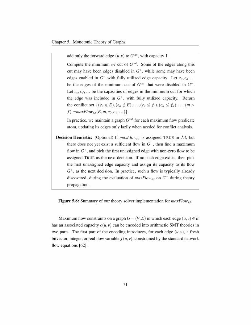
Chapter 5. Monotonic Theory of Graphs
add only the forward edge (u,v) to Gcut , with capacity 1.
Compute the minimum s-t cut of Gcut . Some of the edges along this
cut may have been edges disabled in G+, while some may have been
edges enabled in G+ with fully utilized edge capacity. Let ea,eb, . . .
be the edges of the minimum cut of Gcut that were disabled in G+.
Let cc,cd , . . . be the capacities of edges in the minimum cut for which
the edge was included in G+, with fully utilized capacity. Return
the conflict set (ea /∈ E),(eb /∈ E), . . . ,(cc ≤ fc),(cd ≤ fd), . . . ,(m >
f ),¬maxFlows,t(E,m,c0,c1, . . .).
In practice, we maintain a graph Gcut for each maximum flow predicate
atom, updating its edges only lazily when needed for conflict analysis.
Decision Heuristic: (Optional) If maxFlows,t is assigned TRUE in M, but
there does not yet exist a sufficient flow in G−, then find a maximum
flow in G+, and pick the first unassigned edge with non-zero flow to be
assigned TRUE as the next decision. If no such edge exists, then pick
the first unassigned edge capacity and assign its capacity to its flow
G+, as the next decision. In practice, such a flow is typically already
discovered, during the evaluation of maxFlows,t on G+ during theory
propagation.
Figure 5.8: Summary of our theory solver implementation for maxFlows,t .
Maximum flow constraints on a graph G= (V,E) in which each edge (u,v)∈ E
has an associated capacity c(u,v) can be encoded into arithmetic SMT theories in
two parts. The first part of the encoding introduces, for each edge (u,v), a fresh
bitvector, integer, or real flow variable f (u,v), constrained by the standard network
flow equations [62]:
71

Chapter 5. Monotonic Theory of Graphs
∀u,v ∈V : f (u,v)≤ c(u,v)
∀u ∈V/s, t, ∑v∈V
f (u,v) = ∑w∈V
f (v,w)
∑v∈V
f (s,v)− ∑w∈V
f (w,s) = ∑w∈V
f (w, t)−∑v∈V
f (t,v)
The second part of the encoding non-deterministically selects an s-t cut by
introducing a fresh Boolean variable a(v) for each node v ∈V , with a(v) TRUE iff
v is on the source side of the cut. The sum of the capacities of the edges passing
through that cut are then asserted to be equal to the flow in the graph:
a(s)∧¬a(t) (5.1)
∑v∈V
f (s,v)− ∑w∈V
f (w,s) = ∑(u,v)∈E,a(u)∧¬a(v)
c(u,v) (5.2)
By the max-flow min-cut theorem [86], an s-t flow in a graph is equal to an
s-t cut if and only if that flow is a maximum flow (and the cut a minimum cut).
This encoding is concise (requiring O(|E|+ |V |) arithmetic SMT constraints, or
O(|E| · log |V |+ |V | · log |V |) Boolean variables if a bitvector encoding is used);
unfortunately, the encoding depends on the solver non-deterministically guessing
both a valid flow and a cut in the graph, and in practice scales very poorly (see
Figure 5.9).
72

Chapter 5. Monotonic Theory of Graphs
0 5000 10000 15000 20000 25000 30000 35000 40000# of nodes
0
1
10
100
1000
10000Ti
me
to s
olve
(s)
MonoSATClasp
Figure 5.9: Run-times of MONOSAT and CLASP on maximum flow con-straints. The SMT solver Z3 (using bitvector, integer arithmetic, andlinear arithmetic encodings) times out on all but the smallest instance,so we omit it from this figure. We can also see that CLASP is an or-der of magnitude or more slower than MONOSAT.8In these constraints,randomly chosen edge-capacities (between 5 and 10 units) must be par-titioned between two identical planar, grid-graphs, such that the maxi-mum s-t flow in both graphs (from the top left to the bottom right nodes)is exactly 5. This is an (artificial) example of a multi-commodity flowconstraint, discussed in more detail in Section 6.3.2.
In Figure 5.9 we compare the performance of MONOSAT’s maximum flow
predicate to the performance of Z3 (reporting the best results from linear arith-
metic, integer arithmetic, and bitvector encodings as described above), and to the
performance of CLASP, using a similar encoding into ASP [181].
In this case, Z3 is only able to solve the smallest instance we consider within
a 10,000 second cutoff. We can also see that the encoding into ASP performs
substantially better than Z3, while also being orders of magnitude slower than the
encoding in MONOSAT.
8CLASP is unexpectedly unable to solve some of the smallest instances (top left of Figure 5.9).While I can speculate as to why this is, I do not have a definitive answer.
73
Chapter 5. Monotonic Theory of Graphs
5.4 ConclusionIn this chapter we described our implementations of three important graph predi-
cates in MONOSAT: reachability, acyclicity, and maximum s-t flow. Each of these
predicates is implemented following the techniques described in Chapter 4, and for
each we have demonstrated in this chapter state-of-the-art performance on large,
artificially generated constraints. In Chapter 6, we will describe a series of appli-
cations for these graph predicates, demonstrating that the SMMT framework, as
embodied in MONOSAT, can achieve great improvements in scalability over com-
parable constraint solvers in realistic, rather than artificial, scenarios. MONOSAT
also provides high performance support for several further important graph predi-
cates, including shortest path, connected component count, and minimum spanning
tree weight. The implementations of the theory solvers for these predicates are sim-
ilar to implementations discussed in this chapter, and are summarized in Appendix
D.1.
74
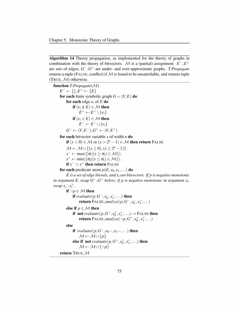
Chapter 5. Monotonic Theory of Graphs
Algorithm 14 Theory propagation, as implemented for the theory of graphs incombination with the theory of bitvectors. M is a (partial) assignment. E−,E+
are sets of edges; G−,G+ are under- and over-approximate graphs. T-Propagatereturns a tuple (FALSE, conflict) ifM is found to be unsatisfiable, and returns tuple(TRUE,M) otherwise.
function T-Propagate(M)E−←,E+←Efor each finite symbolic graph G = (V,E) do
for each edge ei of E doif (ei /∈ E) ∈M then
E+← E+ \eiif (ei ∈ E) ∈M then
E−← E−∪eiG−← (V,E−),G+← (V,E+)
for each bitvector variable x of width n doif (x < 0) ∈M or (x > 2n−1) ∈M then return FALSE
M←M∪(x≥ 0),(x≤ 2n−1)x−←max(σi|(x≥ σi) ∈M).x+←min(σi|(x≤ σi) ∈M).if x− > x+ then return FALSE
for each predicate atom p(E,x0,x1, . . .) doE is a set of edge literals, and xi are bitvectors. If p is negative monotonic
in argument E, swap G−,G+ below; if p is negative monotonic in argument xi,swap x−i ,x
+i .
if ¬p ∈M thenif evaluate(p,G−,x−0 ,x
−1 , . . .) then
return FALSE,analyze(p,G−,x−0 ,x−1 , . . .)
else if p ∈M thenif not evaluate(p,G+,x+0 ,x
+1 , . . .) 7→ FALSE then
return FALSE,analyze(¬p,G+,x+0 ,x+1 , . . .)
elseif evaluate(p,G−,x0−,x1−, . . .) thenM←M∪p
else if not evaluate(p,G+,x+0 ,x+1 , . . .) then
M←M∪¬preturn TRUE,M
75
Chapter 6
Graph Theory Applications
Over the last several chapters, we have claimed that theory solvers implemented
using the techniques we have described in Chapter 4 can have good performance
in practice. Here we describe applications of our theory of graphs (as implemented
in our SMT solver MONOSAT, described in Appendix A) to three different fields,
along with experimental evidence demonstrating that, for the theory of graphs de-
scribed above, we have achieved — and in many cases greatly surpassed — state-
of-the-art performance in each of these different domains.
The first application we consider, procedural content generation, presents re-
sults testing each of the graph predicates described in Chapter 5, demonstrating
MONOSAT’s performance across a diverse set of content generation tasks. The
second and third applications we consider rely on the maximum flow predicate,
and demonstrate MONOSAT’s effectiveness on two industrial applications: circuit
layout and data center allocation. These latter two application scenarios will show
that MONOSAT can effectively solve real-world instances over graphs with hun-
dreds of thousands of nodes and edges — in some cases, even instances with more
than 1 million nodes and edges.
6.1 Procedural Content GenerationThe first application we consider is procedural content generation, in which artistic
objects, such as landscapes or mazes are designed algorithmically, rather than by
76
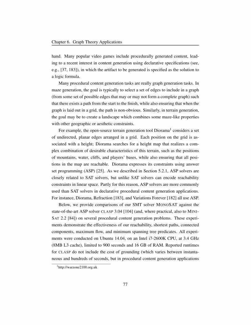
Chapter 6. Graph Theory Applications
hand. Many popular video games include procedurally generated content, lead-
ing to a recent interest in content generation using declarative specifications (see,
e.g., [37, 183]), in which the artifact to be generated is specified as the solution to
a logic formula.
Many procedural content generation tasks are really graph generation tasks. In
maze generation, the goal is typically to select a set of edges to include in a graph
(from some set of possible edges that may or may not form a complete graph) such
that there exists a path from the start to the finish, while also ensuring that when the
graph is laid out in a grid, the path is non-obvious. Similarly, in terrain generation,
the goal may be to create a landscape which combines some maze-like properties
with other geographic or aesthetic constraints.
For example, the open-source terrain generation tool Diorama1 considers a set
of undirected, planar edges arranged in a grid. Each position on the grid is as-
sociated with a height; Diorama searches for a height map that realizes a com-
plex combination of desirable characteristics of this terrain, such as the positions
of mountains, water, cliffs, and players’ bases, while also ensuring that all posi-
tions in the map are reachable. Diorama expresses its constraints using answer
set programming (ASP) [25]. As we described in Section 5.2.1, ASP solvers are
closely related to SAT solvers, but unlike SAT solvers can encode reachability
constraints in linear space. Partly for this reason, ASP solvers are more commonly
used than SAT solvers in declarative procedural content generation applications.
For instance, Diorama, Refraction [183], and Variations Forever [182] all use ASP.
Below, we provide comparisons of our SMT solver MONOSAT against the
state-of-the-art ASP solver CLASP 3.04 [104] (and, where practical, also to MINI-
SAT 2.2 [84]) on several procedural content generation problems. These experi-
ments demonstrate the effectiveness of our reachability, shortest paths, connected
components, maximum flow, and minimum spanning tree predicates. All experi-
ments were conducted on Ubuntu 14.04, on an Intel i7-2600K CPU, at 3.4 GHz
(8MB L3 cache), limited to 900 seconds and 16 GB of RAM. Reported runtimes
for CLASP do not include the cost of grounding (which varies between instanta-
neous and hundreds of seconds, but in procedural content generation applications
1http://warzone2100.org.uk
77
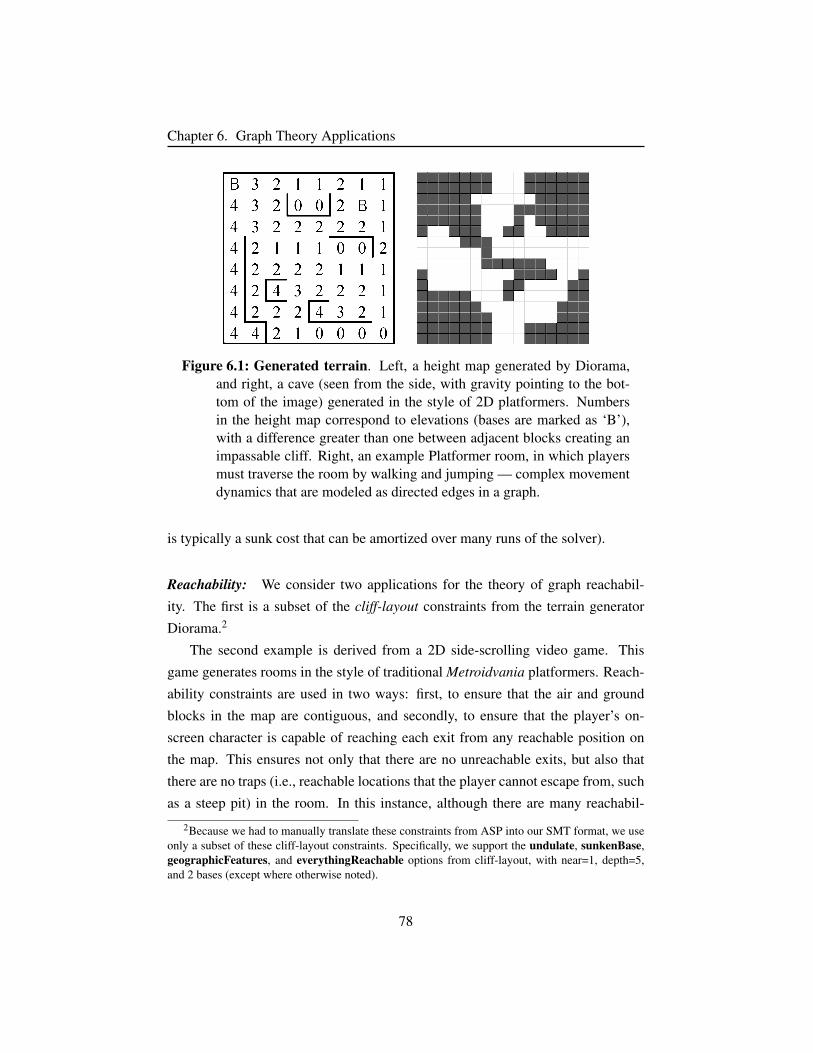
Chapter 6. Graph Theory Applications
Figure 6.1: Generated terrain. Left, a height map generated by Diorama,and right, a cave (seen from the side, with gravity pointing to the bot-tom of the image) generated in the style of 2D platformers. Numbersin the height map correspond to elevations (bases are marked as ‘B’),with a difference greater than one between adjacent blocks creating animpassable cliff. Right, an example Platformer room, in which playersmust traverse the room by walking and jumping — complex movementdynamics that are modeled as directed edges in a graph.
is typically a sunk cost that can be amortized over many runs of the solver).
Reachability: We consider two applications for the theory of graph reachabil-
ity. The first is a subset of the cliff-layout constraints from the terrain generator
Diorama.2
The second example is derived from a 2D side-scrolling video game. This
game generates rooms in the style of traditional Metroidvania platformers. Reach-
ability constraints are used in two ways: first, to ensure that the air and ground
blocks in the map are contiguous, and secondly, to ensure that the player’s on-
screen character is capable of reaching each exit from any reachable position on
the map. This ensures not only that there are no unreachable exits, but also that
there are no traps (i.e., reachable locations that the player cannot escape from, such
as a steep pit) in the room. In this instance, although there are many reachabil-
2Because we had to manually translate these constraints from ASP into our SMT format, we useonly a subset of these cliff-layout constraints. Specifically, we support the undulate, sunkenBase,geographicFeatures, and everythingReachable options from cliff-layout, with near=1, depth=5,and 2 bases (except where otherwise noted).
78
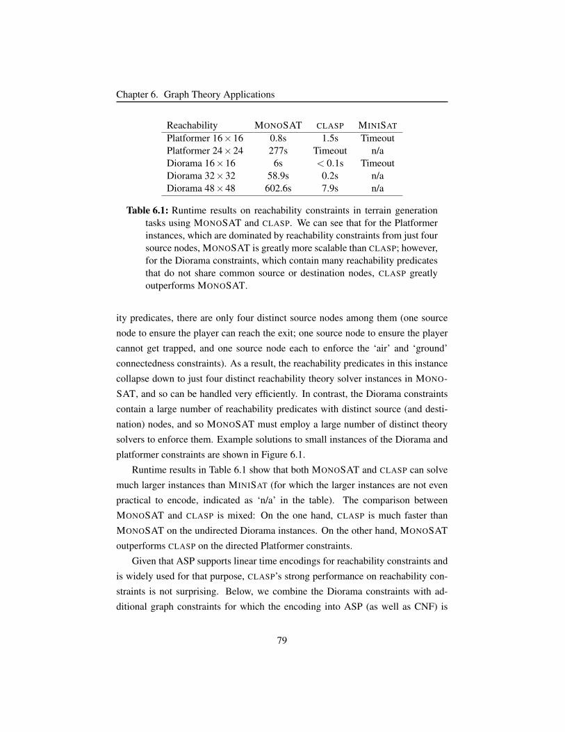
Chapter 6. Graph Theory Applications
Reachability MONOSAT CLASP MINISAT
Platformer 16×16 0.8s 1.5s TimeoutPlatformer 24×24 277s Timeout n/aDiorama 16×16 6s < 0.1s TimeoutDiorama 32×32 58.9s 0.2s n/aDiorama 48×48 602.6s 7.9s n/a
Table 6.1: Runtime results on reachability constraints in terrain generationtasks using MONOSAT and CLASP. We can see that for the Platformerinstances, which are dominated by reachability constraints from just foursource nodes, MONOSAT is greatly more scalable than CLASP; however,for the Diorama constraints, which contain many reachability predicatesthat do not share common source or destination nodes, CLASP greatlyoutperforms MONOSAT.
ity predicates, there are only four distinct source nodes among them (one source
node to ensure the player can reach the exit; one source node to ensure the player
cannot get trapped, and one source node each to enforce the ‘air’ and ‘ground’
connectedness constraints). As a result, the reachability predicates in this instance
collapse down to just four distinct reachability theory solver instances in MONO-
SAT, and so can be handled very efficiently. In contrast, the Diorama constraints
contain a large number of reachability predicates with distinct source (and desti-
nation) nodes, and so MONOSAT must employ a large number of distinct theory
solvers to enforce them. Example solutions to small instances of the Diorama and
platformer constraints are shown in Figure 6.1.
Runtime results in Table 6.1 show that both MONOSAT and CLASP can solve
much larger instances than MINISAT (for which the larger instances are not even
practical to encode, indicated as ‘n/a’ in the table). The comparison between
MONOSAT and CLASP is mixed: On the one hand, CLASP is much faster than
MONOSAT on the undirected Diorama instances. On the other hand, MONOSAT
outperforms CLASP on the directed Platformer constraints.
Given that ASP supports linear time encodings for reachability constraints and
is widely used for that purpose, CLASP’s strong performance on reachability con-
straints is not surprising. Below, we combine the Diorama constraints with ad-
ditional graph constraints for which the encoding into ASP (as well as CNF) is
79
Chapter 6. Graph Theory Applications
Size Range MONOSAT CLASP MINISAT
8×8 8-16 <0.1s <0.1s 9s16×16 16-32 4s 7s >3600s16×16 32-48 4s 23s 2096s16×16 32-64 4s 65s >3600s16×16 32-96 4s >3600s >3600s16×16 32-128 4s >3600s >3600s24×24 48-64 46s 30s >3600s24×24 48-96 61s 1125s >3600s32×32 64-128 196s >3600s >3600s
Table 6.2: Runtime results for shortest paths constraints in Diorama. Here,we can see that both as the size of the map is increased, and as the lengthsof the shortest path constraints are increased, MONOSAT outperformsCLASP.
non-linear, and in each case MONOSAT outperforms CLASP, as well as MINISAT
dramatically.
Shortest Paths: We consider a modified version of the Diorama terrain genera-
tor, replacing the reachability constraint with the constraint that the shortest path
between the two bases must fall within a certain range (‘Range’, in Figure 6.2). We
tested this constraint while enforcing an increasingly large set of ranges, and also
while testing larger Diorama graph sizes (8× 8,16× 16,24× 24,32× 32). One
can see that while ASP is competitive with MONOSAT in smaller graphs and with
smaller shortest-path range constraints, both as the size of the shortest path range
constraint increases, and also as the size of the graph itself increases, the encodings
of shortest path constraints in both SAT and ASP scale poorly.
The two-sided encoding for shortest paths into CNF that we compare to here
is to symbolically unroll the Floyd-Warshall algorithm (similar to encoding two-
sided reachability constraints). A shortest path predicate shortestPaths,t(G) ≤ L,
which evaluates to TRUE iff the shortest path in G is less than or equal to constant
L, can be encoded into CNF using O(L · |E| · |V |) clauses (with E the set of edges,
and V the set of vertices, in G). This encoding is practical only for very small
graphs, or for small, constant values of L (as can be seen in the performance of
80
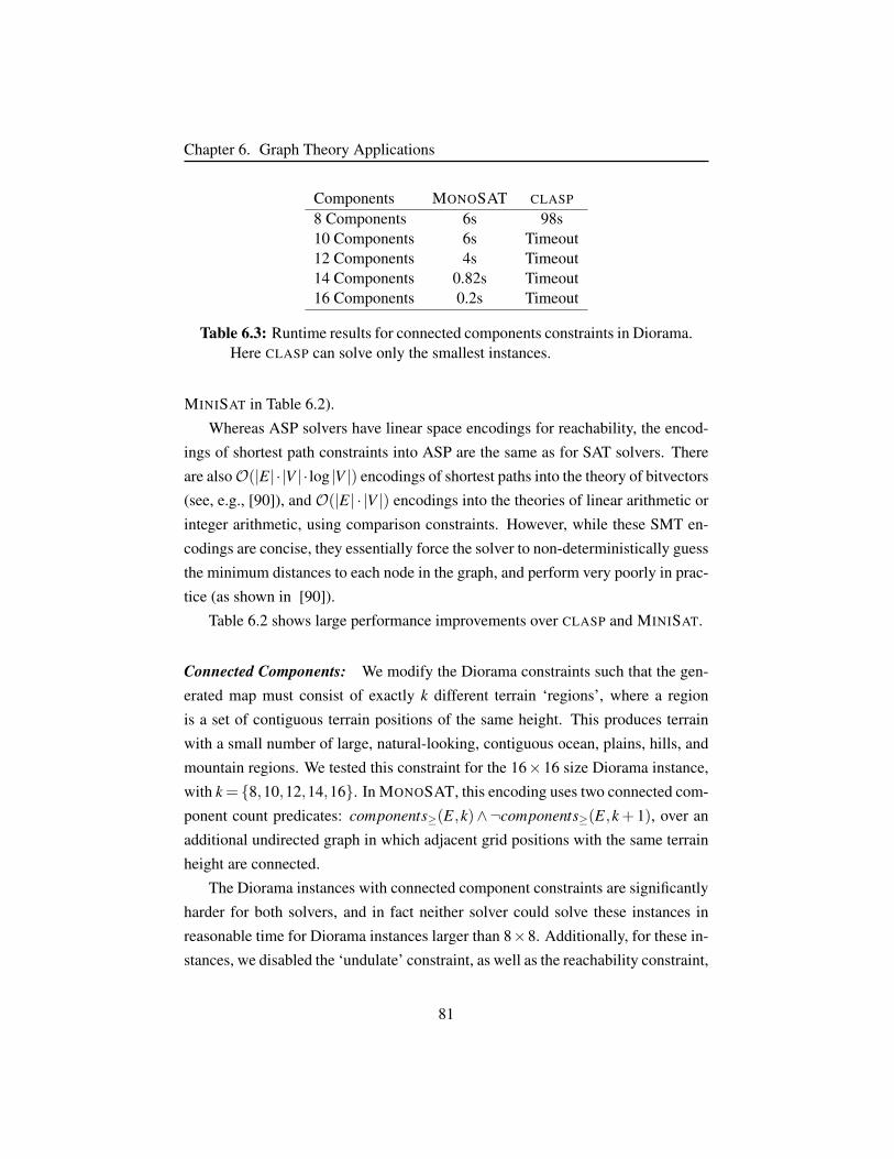
Chapter 6. Graph Theory Applications
Components MONOSAT CLASP
8 Components 6s 98s10 Components 6s Timeout12 Components 4s Timeout14 Components 0.82s Timeout16 Components 0.2s Timeout
Table 6.3: Runtime results for connected components constraints in Diorama.Here CLASP can solve only the smallest instances.
MINISAT in Table 6.2).
Whereas ASP solvers have linear space encodings for reachability, the encod-
ings of shortest path constraints into ASP are the same as for SAT solvers. There
are alsoO(|E| · |V | · log |V |) encodings of shortest paths into the theory of bitvectors
(see, e.g., [90]), and O(|E| · |V |) encodings into the theories of linear arithmetic or
integer arithmetic, using comparison constraints. However, while these SMT en-
codings are concise, they essentially force the solver to non-deterministically guess
the minimum distances to each node in the graph, and perform very poorly in prac-
tice (as shown in [90]).
Table 6.2 shows large performance improvements over CLASP and MINISAT.
Connected Components: We modify the Diorama constraints such that the gen-
erated map must consist of exactly k different terrain ‘regions’, where a region
is a set of contiguous terrain positions of the same height. This produces terrain
with a small number of large, natural-looking, contiguous ocean, plains, hills, and
mountain regions. We tested this constraint for the 16×16 size Diorama instance,
with k = 8,10,12,14,16. In MONOSAT, this encoding uses two connected com-
ponent count predicates: components≥(E,k)∧¬components≥(E,k+ 1), over an
additional undirected graph in which adjacent grid positions with the same terrain
height are connected.
The Diorama instances with connected component constraints are significantly
harder for both solvers, and in fact neither solver could solve these instances in
reasonable time for Diorama instances larger than 8×8. Additionally, for these in-
stances, we disabled the ‘undulate’ constraint, as well as the reachability constraint,
81
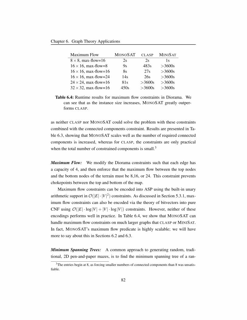
Chapter 6. Graph Theory Applications
Maximum Flow MONOSAT CLASP MINISAT
8×8, max-flow=16 2s 2s 1s16×16, max-flow=8 9s 483s >3600s16×16, max-flow=16 8s 27s >3600s16×16, max-flow=24 14s 26s >3600s24×24, max-flow=16 81s >3600s >3600s32×32, max-flow=16 450s >3600s >3600s
Table 6.4: Runtime results for maximum flow constraints in Diorama. Wecan see that as the instance size increases, MONOSAT greatly outper-forms CLASP.
as neither CLASP nor MONOSAT could solve the problem with these constraints
combined with the connected components constraint. Results are presented in Ta-
ble 6.3, showing that MONOSAT scales well as the number of required connected
components is increased, whereas for CLASP, the constraints are only practical
when the total number of constrained components is small.3
Maximum Flow: We modify the Diorama constraints such that each edge has
a capacity of 4, and then enforce that the maximum flow between the top nodes
and the bottom nodes of the terrain must be 8,16, or 24. This constraint prevents
chokepoints between the top and bottom of the map.
Maximum flow constraints can be encoded into ASP using the built-in unary
arithmetic support inO(|E| · |V |2) constraints. As discussed in Section 5.3.1, max-
imum flow constraints can also be encoded via the theory of bitvectors into pure
CNF using O(|E| · log |V |+ |V | · log |V |) constraints. However, neither of these
encodings performs well in practice. In Table 6.4, we show that MONOSAT can
handle maximum flow constraints on much larger graphs that CLASP or MINISAT.
In fact, MONOSAT’s maximum flow predicate is highly scalable; we will have
more to say about this in Sections 6.2 and 6.3.
Minimum Spanning Trees: A common approach to generating random, tradi-
tional, 2D pen-and-paper mazes, is to find the minimum spanning tree of a ran-
3The entries begin at 8, as forcing smaller numbers of connected components than 8 was unsatis-fiable.
82
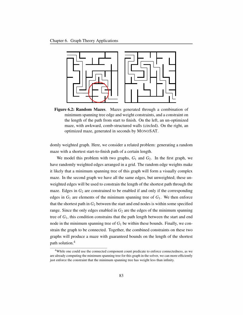
Chapter 6. Graph Theory Applications
Figure 6.2: Random Mazes. Mazes generated through a combination ofminimum spanning tree edge and weight constraints, and a constraint onthe length of the path from start to finish. On the left, an un-optimizedmaze, with awkward, comb-structured walls (circled). On the right, anoptimized maze, generated in seconds by MONOSAT.
domly weighted graph. Here, we consider a related problem: generating a random
maze with a shortest start-to-finish path of a certain length.
We model this problem with two graphs, G1 and G2. In the first graph, we
have randomly weighted edges arranged in a grid. The random edge weights make
it likely that a minimum spanning tree of this graph will form a visually complex
maze. In the second graph we have all the same edges, but unweighted; these un-
weighted edges will be used to constrain the length of the shortest path through the
maze. Edges in G2 are constrained to be enabled if and only if the corresponding
edges in G1 are elements of the minimum spanning tree of G1. We then enforce
that the shortest path in G2 between the start and end nodes is within some specified
range. Since the only edges enabled in G2 are the edges of the minimum spanning
tree of G1, this condition constrains that the path length between the start and end
node in the minimum spanning tree of G1 be within these bounds. Finally, we con-
strain the graph to be connected. Together, the combined constraints on these two
graphs will produce a maze with guaranteed bounds on the length of the shortest
path solution.4
4While one could use the connected component count predicate to enforce connectedness, as weare already computing the minimum spanning tree for this graph in the solver, we can more efficientlyjust enforce the constraint that the minimum spanning tree has weight less than infinity.
83

Chapter 6. Graph Theory Applications
Spanning Tree MONOSAT CLASP
Maze 5×5 < 0.1s 15sMaze 8×8 1.5s TimeoutMaze 16×16 32s Timeout
Table 6.5: Runtime results for maze generation using minimum spanning treeconstraints, comparing MONOSAT and CLASP. In these instances, theshortest path through the maze was constrained to a length between 3and 4 times the width of the maze.
The solver must select a set of edges in G1 to enable and disable such that
the minimum spanning tree of the resulting graph is a) connected and b) results
in a maze with a shortest start-to-finish path within the requested bounds. By it-
self, these constraints can result in poor-quality mazes (see Figure 6.2, left, and
notice the unnatural wall formations circled in red); by allowing the edges in G1
to be enabled or disabled freely, any tree can become the minimum spanning tree,
effectively eliminating the effect of the random edge weight constraints.
Instead we convert this into an optimization problem, by combining it with an
additional constraint: that the minimum spanning tree of G1 must be ≤ to some
constant, which we then lower repeatedly until it cannot be lowered any further
without making the instance unsatisfiable.5 This produces plausible mazes (see
Figure 6.2, right), while also satisfying the shortest path constraints, and can be
solved in reasonable time using MONOSAT (Figure 6.5).
5MONOSAT has built-in support for optimization problems via linear or binary search, andCLASP supports minimization via the “#minimize” statement.
84
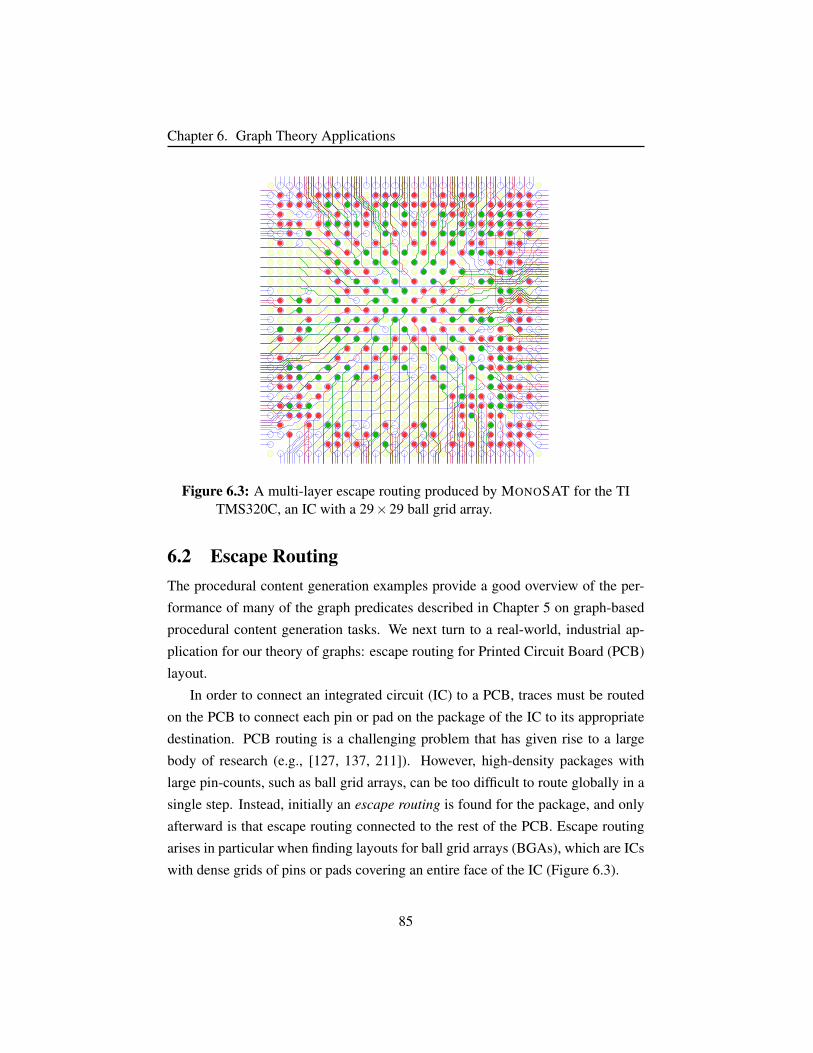
Chapter 6. Graph Theory Applications
Figure 6.3: A multi-layer escape routing produced by MONOSAT for the TITMS320C, an IC with a 29×29 ball grid array.
6.2 Escape RoutingThe procedural content generation examples provide a good overview of the per-
formance of many of the graph predicates described in Chapter 5 on graph-based
procedural content generation tasks. We next turn to a real-world, industrial ap-
plication for our theory of graphs: escape routing for Printed Circuit Board (PCB)
layout.
In order to connect an integrated circuit (IC) to a PCB, traces must be routed
on the PCB to connect each pin or pad on the package of the IC to its appropriate
destination. PCB routing is a challenging problem that has given rise to a large
body of research (e.g., [127, 137, 211]). However, high-density packages with
large pin-counts, such as ball grid arrays, can be too difficult to route globally in a
single step. Instead, initially an escape routing is found for the package, and only
afterward is that escape routing connected to the rest of the PCB. Escape routing
arises in particular when finding layouts for ball grid arrays (BGAs), which are ICs
with dense grids of pins or pads covering an entire face of the IC (Figure 6.3).
85
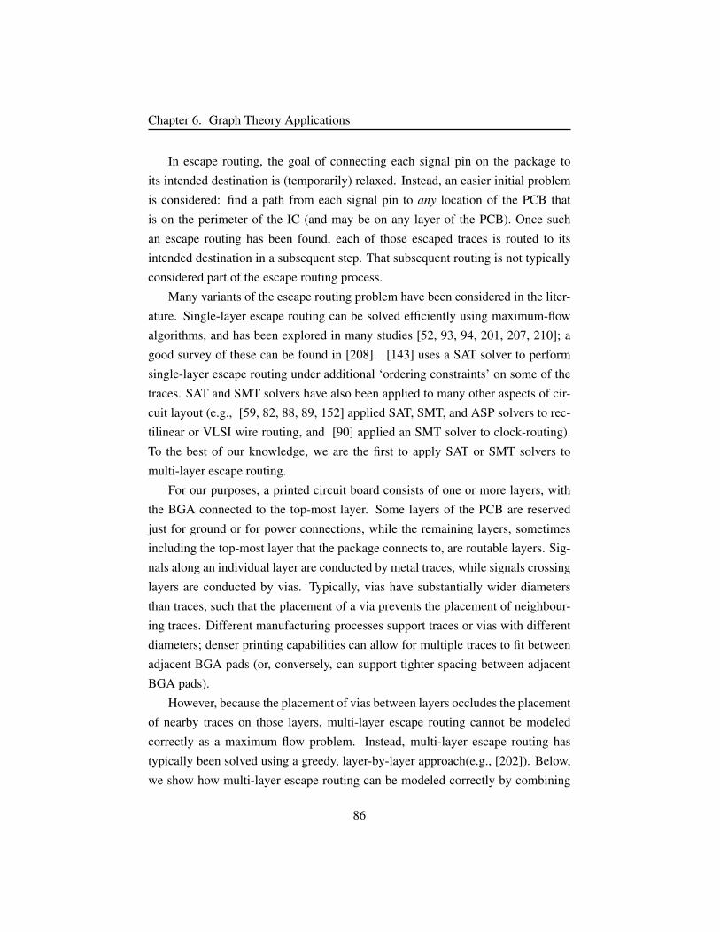
Chapter 6. Graph Theory Applications
In escape routing, the goal of connecting each signal pin on the package to
its intended destination is (temporarily) relaxed. Instead, an easier initial problem
is considered: find a path from each signal pin to any location of the PCB that
is on the perimeter of the IC (and may be on any layer of the PCB). Once such
an escape routing has been found, each of those escaped traces is routed to its
intended destination in a subsequent step. That subsequent routing is not typically
considered part of the escape routing process.
Many variants of the escape routing problem have been considered in the liter-
ature. Single-layer escape routing can be solved efficiently using maximum-flow
algorithms, and has been explored in many studies [52, 93, 94, 201, 207, 210]; a
good survey of these can be found in [208]. [143] uses a SAT solver to perform
single-layer escape routing under additional ‘ordering constraints’ on some of the
traces. SAT and SMT solvers have also been applied to many other aspects of cir-
cuit layout (e.g., [59, 82, 88, 89, 152] applied SAT, SMT, and ASP solvers to rec-
tilinear or VLSI wire routing, and [90] applied an SMT solver to clock-routing).
To the best of our knowledge, we are the first to apply SAT or SMT solvers to
multi-layer escape routing.
For our purposes, a printed circuit board consists of one or more layers, with
the BGA connected to the top-most layer. Some layers of the PCB are reserved
just for ground or for power connections, while the remaining layers, sometimes
including the top-most layer that the package connects to, are routable layers. Sig-
nals along an individual layer are conducted by metal traces, while signals crossing
layers are conducted by vias. Typically, vias have substantially wider diameters
than traces, such that the placement of a via prevents the placement of neighbour-
ing traces. Different manufacturing processes support traces or vias with different
diameters; denser printing capabilities can allow for multiple traces to fit between
adjacent BGA pads (or, conversely, can support tighter spacing between adjacent
BGA pads).
However, because the placement of vias between layers occludes the placement
of nearby traces on those layers, multi-layer escape routing cannot be modeled
correctly as a maximum flow problem. Instead, multi-layer escape routing has
typically been solved using a greedy, layer-by-layer approach(e.g., [202]). Below,
we show how multi-layer escape routing can be modeled correctly by combining
86

Chapter 6. Graph Theory Applications
Figure 6.4: Multi-layer escape routing with simultaneous via-placement. On-grid positions are shown as large nodes, while 45-degree traces passthrough the small nodes. This is a symbolic graph, in which some of thenodes or edges in this graph are included only if corresponding Booleanvariables in an associated formula φ are assigned TRUE. We constructφ such that nodes connecting adjacent layers (the central black node,representing a via) are included in the graph only if the nodes surround-ing the via (marked in gray) are disabled. The via node (center, black)is connected to all nodes around the periphery of the gray nodes, as wellas to the central node (interior to the gray nodes).
the maximum flow predicate of Chapter 5 with additional Boolean constraints, and
solved efficiently using MONOSAT.
6.2.1 Multi-Layer Escape Routing in MONOSAT
Figure 6.4 illustrates the symbolic flow graph we use to model multi-layer escape
routing. Each layer of this flow-graph is similar to typical single-layer network
flow-based escape routing solutions (see, e.g., [207]), except that in our graph
all positions are potentially routable, with no spaces reserved for vias or pads.
Each node in the graph has a node capacity of 1 (with node capacities enforced by
introducing pairs of nodes connected by a single edge of capacity 1).
We also include potential vias in the graph, spaced at regular intervals, that
the solver may choose to include or exclude from the graph. The potential via
is shown as a black node in Figure 6.4, with neighbouring nodes shown in gray,
indicating that they would be blocked by that via. In Figure 6.4, we show in gray
the nodes that would be blocked by a via with a radius roughly 1.5 times the width
of a trace. However, different via widths can be easily supported by simply altering
the pattern of gray nodes to be blocked by the via.
87
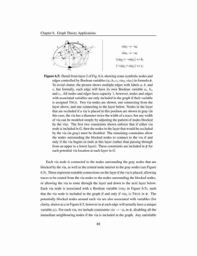
Chapter 6. Graph Theory Applications
b
bb
bb
b
cc c c c c c
b
aa
aa
aaa
a
via2
via3
via2→¬ai
via3→¬ai
(via2∧¬via3)↔ bi
(¬via2∧ via3)↔ ci
Figure 6.5: Detail from layer 2 of Fig. 6.4, showing some symbolic nodes andedges controlled by Boolean variables (ai,bi,ci,via2,via3) in formula φ .To avoid clutter, the picture shows multiple edges with labels a, b, andc, but formally, each edge will have its own Boolean variable ai, bi,and ci. All nodes and edges have capacity 1, however, nodes and edgeswith associated variables are only included in the graph if their variableis assigned TRUE. Two via nodes are shown, one connecting from thelayer above, and one connecting to the layer below. Nodes in the layerthat are occluded if a via is placed in this position are shown in gray (inthis case, the via has a diameter twice the width of a trace, but any widthof via can be modeled simply by adjusting the pattern of nodes blockedby the via). The first two constraints shown enforce that if either vianode is included in G, then the nodes in the layer that would be occludedby the via (in gray) must be disabled. The remaining constraints allowthe nodes surrounding the blocked nodes to connect to the via if andonly if the via begins or ends at this layer (rather than passing throughfrom an upper to a lower layer). These constraints are included in φ foreach potential via location at each layer in G.
Each via node is connected to the nodes surrounding the gray nodes that are
blocked by the via, as well as the central node interior to the gray nodes (see Figure
6.5). These represent routable connections on the layer if the via is placed, allowing
traces to be routed from the via nodes to the nodes surrounding the blocked nodes,
or allowing the via to route through the layer and down to the next layer below.
Each via node is associated with a Boolean variable (via2 in Figure 6.5), such
that the via node is included in the graph if and only if via2 is TRUE in φ . The
potentially blocked nodes around each via are also associated with variables (for
clarity, drawn as a in Figure 6.5, however in φ each edge will actually have a unique
variable ai). For each via, we include constraints via→¬ai in φ , disabling all the
immediate neighbouring nodes if the via is included in the graph. Any satisfiable
88
Chapter 6. Graph Theory Applications
assignment to these constraints in φ selects a subset of the nodes of G representing
a compatible, non-overlapping set of vias and traces.
Four configurations are possible for the two via nodes shown in Figure 6.5: (a)
neither via node is enabled, allowing traces to be routed through the gray nodes
on this layer, (b) the via enters from above, and connects to this layer, (c) the via
begins at this layer, connecting to a layer below, and (d) the via passes through this
layer, connecting the layer above to the layer below. By adding constraints restrict-
ing the allowable configurations of vias, as described in Figure 6.6, our approach
can model all the commonly used via types: through-hole vias, buried vias, blind
vias, or any-layer micro-vias. With minor adjustments to the constraints, these dif-
ferent via types can be combined into a single model or can be restricted to specific
layers of the PCB, allowing a wide variety of PCB manufacturing processes to be
supported.
We add an additional source node s and sink node t to the graph, with di-
rected, capacity-1 edges connecting the s to each signal in the graph, and directed,
capacity-1 edges connecting all nodes on the perimeter of each layer to t. Finally,
a single flow constraint max f lows,t(E) ≥ |signals| is added to φ , ensuring that in
any satisfying assignment, the subset of edges included in the graph must admit a
flow corresponding to a valid escape routing for all of the signal pins.
A solution to this formula corresponds to a feasible multi-layer escape routing,
including via and trace placement. However, as MONOSAT only supports maxi-
mum flow constraints, and not minimum-cost maximum flow constraints, the trace
routing in this solution is typically far from optimal (with traces making completely
unnecessary detours, for example). For this reason, once MONOSAT has produced
a feasible escape routing, including a placement of each via, we then apply an off-
the-shelf minimum-cost maximum flow solver [165] to find a corresponding locally
optimal trace routing for each individual layer of the feasible routing. This can be
solved using completely standard linear-programming encodings of minimum-cost
maximum flow, as the vias are already placed and the layer that each signal is to be
routed on is already known.
89
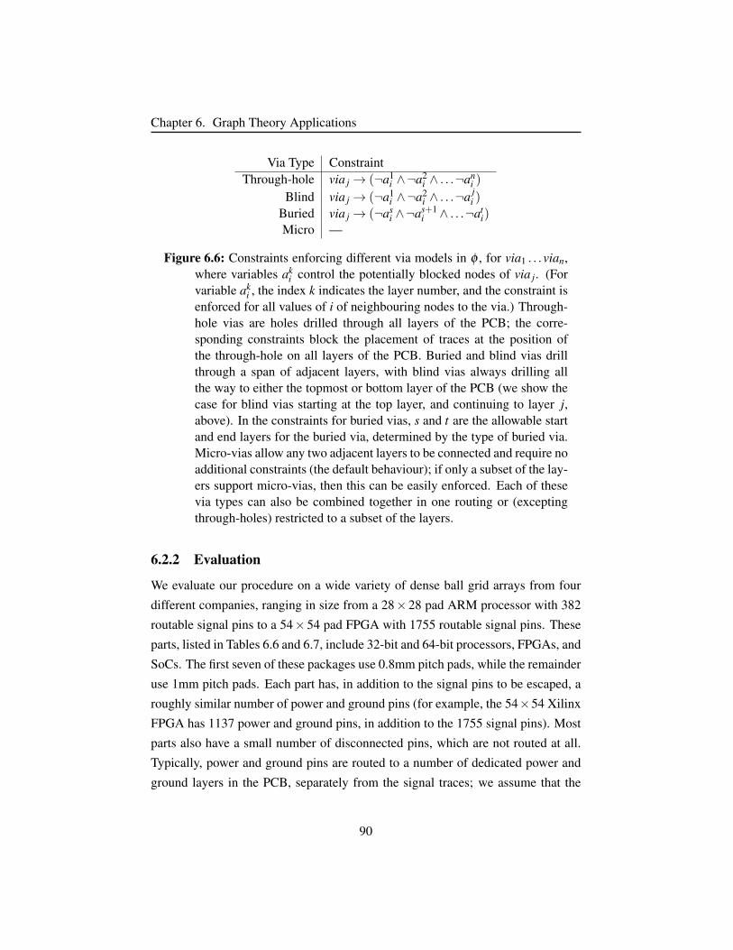
Chapter 6. Graph Theory Applications
Via Type ConstraintThrough-hole via j→ (¬a1
i ∧¬a2i ∧ . . .¬an
i )
Blind via j→ (¬a1i ∧¬a2
i ∧ . . .¬a ji )
Buried via j→ (¬asi ∧¬as+1
i ∧ . . .¬ati)
Micro —
Figure 6.6: Constraints enforcing different via models in φ , for via1 . . .vian,where variables ak
i control the potentially blocked nodes of via j. (Forvariable ak
i , the index k indicates the layer number, and the constraint isenforced for all values of i of neighbouring nodes to the via.) Through-hole vias are holes drilled through all layers of the PCB; the corre-sponding constraints block the placement of traces at the position ofthe through-hole on all layers of the PCB. Buried and blind vias drillthrough a span of adjacent layers, with blind vias always drilling allthe way to either the topmost or bottom layer of the PCB (we show thecase for blind vias starting at the top layer, and continuing to layer j,above). In the constraints for buried vias, s and t are the allowable startand end layers for the buried via, determined by the type of buried via.Micro-vias allow any two adjacent layers to be connected and require noadditional constraints (the default behaviour); if only a subset of the lay-ers support micro-vias, then this can be easily enforced. Each of thesevia types can also be combined together in one routing or (exceptingthrough-holes) restricted to a subset of the layers.
6.2.2 Evaluation
We evaluate our procedure on a wide variety of dense ball grid arrays from four
different companies, ranging in size from a 28×28 pad ARM processor with 382
routable signal pins to a 54×54 pad FPGA with 1755 routable signal pins. These
parts, listed in Tables 6.6 and 6.7, include 32-bit and 64-bit processors, FPGAs, and
SoCs. The first seven of these packages use 0.8mm pitch pads, while the remainder
use 1mm pitch pads. Each part has, in addition to the signal pins to be escaped, a
roughly similar number of power and ground pins (for example, the 54×54 Xilinx
FPGA has 1137 power and ground pins, in addition to the 1755 signal pins). Most
parts also have a small number of disconnected pins, which are not routed at all.
Typically, power and ground pins are routed to a number of dedicated power and
ground layers in the PCB, separately from the signal traces; we assume that the
90
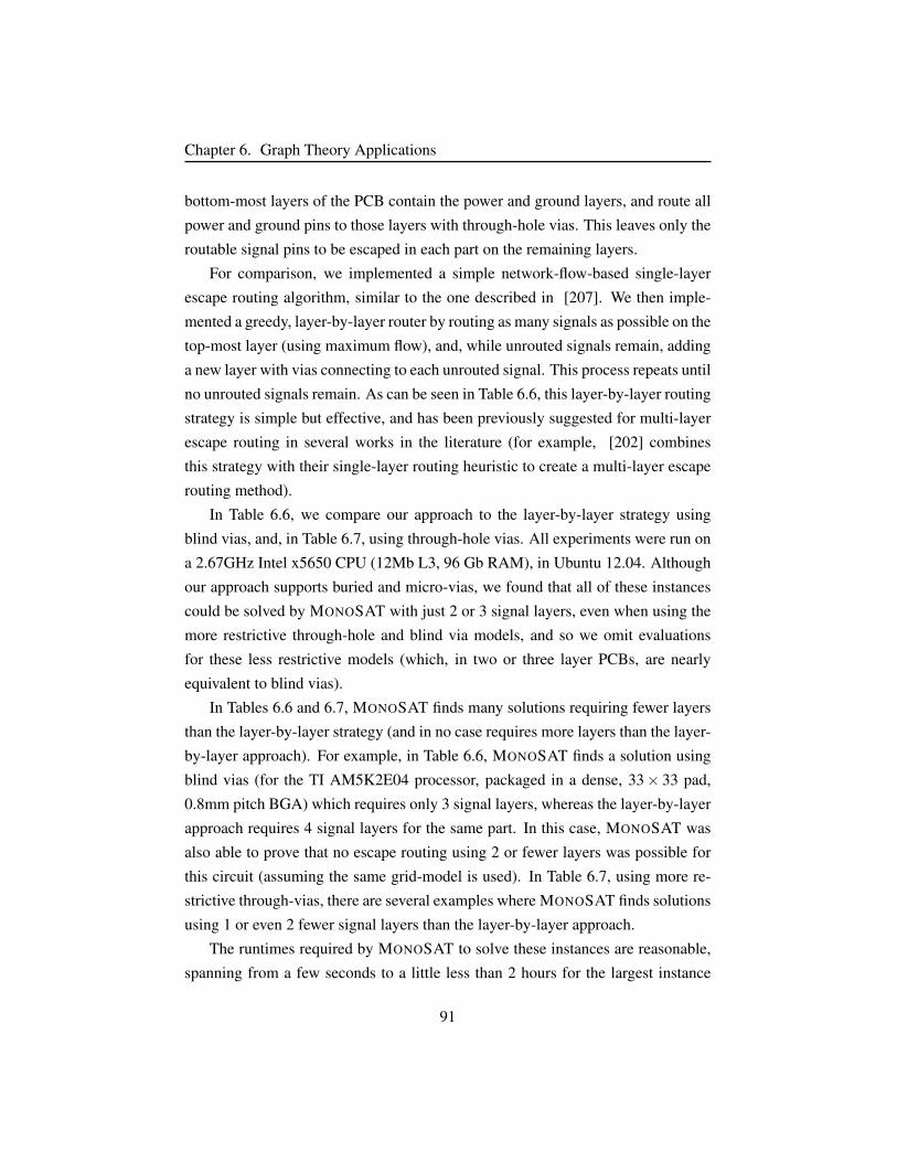
Chapter 6. Graph Theory Applications
bottom-most layers of the PCB contain the power and ground layers, and route all
power and ground pins to those layers with through-hole vias. This leaves only the
routable signal pins to be escaped in each part on the remaining layers.
For comparison, we implemented a simple network-flow-based single-layer
escape routing algorithm, similar to the one described in [207]. We then imple-
mented a greedy, layer-by-layer router by routing as many signals as possible on the
top-most layer (using maximum flow), and, while unrouted signals remain, adding
a new layer with vias connecting to each unrouted signal. This process repeats until
no unrouted signals remain. As can be seen in Table 6.6, this layer-by-layer routing
strategy is simple but effective, and has been previously suggested for multi-layer
escape routing in several works in the literature (for example, [202] combines
this strategy with their single-layer routing heuristic to create a multi-layer escape
routing method).
In Table 6.6, we compare our approach to the layer-by-layer strategy using
blind vias, and, in Table 6.7, using through-hole vias. All experiments were run on
a 2.67GHz Intel x5650 CPU (12Mb L3, 96 Gb RAM), in Ubuntu 12.04. Although
our approach supports buried and micro-vias, we found that all of these instances
could be solved by MONOSAT with just 2 or 3 signal layers, even when using the
more restrictive through-hole and blind via models, and so we omit evaluations
for these less restrictive models (which, in two or three layer PCBs, are nearly
equivalent to blind vias).
In Tables 6.6 and 6.7, MONOSAT finds many solutions requiring fewer layers
than the layer-by-layer strategy (and in no case requires more layers than the layer-
by-layer approach). For example, in Table 6.6, MONOSAT finds a solution using
blind vias (for the TI AM5K2E04 processor, packaged in a dense, 33× 33 pad,
0.8mm pitch BGA) which requires only 3 signal layers, whereas the layer-by-layer
approach requires 4 signal layers for the same part. In this case, MONOSAT was
also able to prove that no escape routing using 2 or fewer layers was possible for
this circuit (assuming the same grid-model is used). In Table 6.7, using more re-
strictive through-vias, there are several examples where MONOSAT finds solutions
using 1 or even 2 fewer signal layers than the layer-by-layer approach.
The runtimes required by MONOSAT to solve these instances are reasonable,
spanning from a few seconds to a little less than 2 hours for the largest instance
91
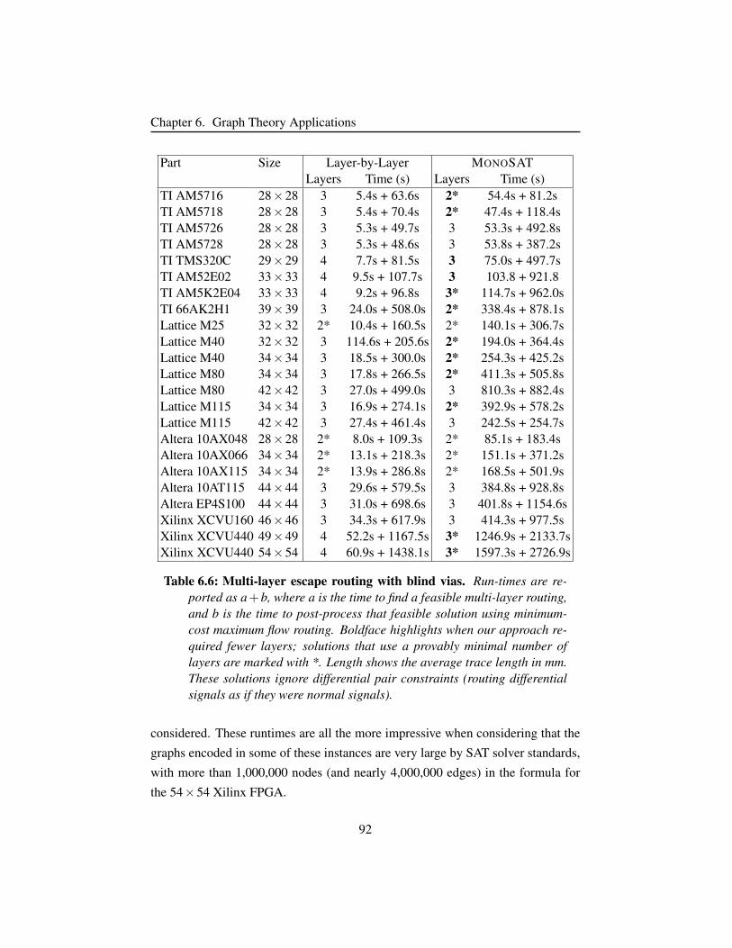
Chapter 6. Graph Theory Applications
Part Size Layer-by-Layer MONOSATLayers Time (s) Layers Time (s)
TI AM5716 28×28 3 5.4s + 63.6s 2* 54.4s + 81.2sTI AM5718 28×28 3 5.4s + 70.4s 2* 47.4s + 118.4sTI AM5726 28×28 3 5.3s + 49.7s 3 53.3s + 492.8sTI AM5728 28×28 3 5.3s + 48.6s 3 53.8s + 387.2sTI TMS320C 29×29 4 7.7s + 81.5s 3 75.0s + 497.7sTI AM52E02 33×33 4 9.5s + 107.7s 3 103.8 + 921.8TI AM5K2E04 33×33 4 9.2s + 96.8s 3* 114.7s + 962.0sTI 66AK2H1 39×39 3 24.0s + 508.0s 2* 338.4s + 878.1sLattice M25 32×32 2* 10.4s + 160.5s 2* 140.1s + 306.7sLattice M40 32×32 3 114.6s + 205.6s 2* 194.0s + 364.4sLattice M40 34×34 3 18.5s + 300.0s 2* 254.3s + 425.2sLattice M80 34×34 3 17.8s + 266.5s 2* 411.3s + 505.8sLattice M80 42×42 3 27.0s + 499.0s 3 810.3s + 882.4sLattice M115 34×34 3 16.9s + 274.1s 2* 392.9s + 578.2sLattice M115 42×42 3 27.4s + 461.4s 3 242.5s + 254.7sAltera 10AX048 28×28 2* 8.0s + 109.3s 2* 85.1s + 183.4sAltera 10AX066 34×34 2* 13.1s + 218.3s 2* 151.1s + 371.2sAltera 10AX115 34×34 2* 13.9s + 286.8s 2* 168.5s + 501.9sAltera 10AT115 44×44 3 29.6s + 579.5s 3 384.8s + 928.8sAltera EP4S100 44×44 3 31.0s + 698.6s 3 401.8s + 1154.6sXilinx XCVU160 46×46 3 34.3s + 617.9s 3 414.3s + 977.5sXilinx XCVU440 49×49 4 52.2s + 1167.5s 3* 1246.9s + 2133.7sXilinx XCVU440 54×54 4 60.9s + 1438.1s 3* 1597.3s + 2726.9s
Table 6.6: Multi-layer escape routing with blind vias. Run-times are re-ported as a+b, where a is the time to find a feasible multi-layer routing,and b is the time to post-process that feasible solution using minimum-cost maximum flow routing. Boldface highlights when our approach re-quired fewer layers; solutions that use a provably minimal number oflayers are marked with *. Length shows the average trace length in mm.These solutions ignore differential pair constraints (routing differentialsignals as if they were normal signals).
considered. These runtimes are all the more impressive when considering that the
graphs encoded in some of these instances are very large by SAT solver standards,
with more than 1,000,000 nodes (and nearly 4,000,000 edges) in the formula for
the 54×54 Xilinx FPGA.
92
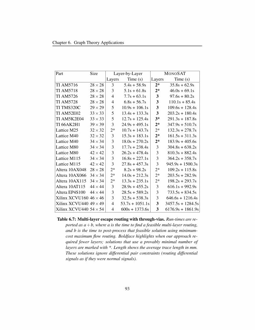
Chapter 6. Graph Theory Applications
Part Size Layer-by-Layer MONOSATLayers Time (s) Layers Time (s)
TI AM5716 28×28 3 5.4s + 58.9s 2* 35.8s + 62.9sTI AM5718 28×28 3 5.1s + 61.8s 2* 46.0s + 69.1sTI AM5726 28×28 4 7.7s + 63.1s 3 97.6s + 80.2sTI AM5728 28×28 4 6.8s + 56.7s 3 110.1s + 85.4sTI TMS320C 29×29 5 10.9s + 106.1s 3 109.6s + 128.4sTI AM52E02 33×33 5 13.4s + 133.3s 3 203.2s + 180.4sTI AM5K2E04 33×33 5 12.7s + 125.4s 3* 291.3s + 187.8sTI 66AK2H1 39×39 3 24.9s + 495.1s 2* 347.9s + 510.7sLattice M25 32×32 2* 10.7s + 143.7s 2* 132.3s + 278.7sLattice M40 32×32 3 15.3s + 183.1s 2* 161.5s + 311.3sLattice M40 34×34 3 18.0s + 270.2s 2* 183.9s + 405.6sLattice M80 34×34 3 17.7s + 238.4s 3 304.8s + 638.2sLattice M80 42×42 3 26.2s + 478.4s 3 810.3s + 882.4sLattice M115 34×34 3 16.8s + 227.1s 3 364.2s + 358.7sLattice M115 42×42 3 27.8s + 457.3s 3 945.9s + 1500.3sAltera 10AX048 28×28 2* 8.2s + 98.2s 2* 109.2s + 115.8sAltera 10AX066 34×34 2* 14.0s + 212.3s 2* 203.5s + 282.9sAltera 10AX115 34×34 2* 13.3s + 235.1s 2* 198.2s + 293.7sAltera 10AT115 44×44 3 28.9s + 455.2s 3 616.1s + 992.9sAltera EP4S100 44×44 3 28.5s + 589.2s 3 733.5s + 834.5sXilinx XCVU160 46×46 3 32.5s + 538.3s 3 646.6s + 1216.4sXilinx XCVU440 49×49 4 53.7s + 1051.1s 3 3457.5s + 1284.5sXilinx XCVU440 54×54 4 600s + 1373.6s 3 6176.9s + 1861.9s
Table 6.7: Multi-layer escape routing with through-vias. Run-times are re-ported as a+b, where a is the time to find a feasible multi-layer routing,and b is the time to post-process that feasible solution using minimum-cost maximum flow routing. Boldface highlights when our approach re-quired fewer layers; solutions that use a provably minimal number oflayers are marked with *. Length shows the average trace length in mm.These solutions ignore differential pair constraints (routing differentialsignals as if they were normal signals).
93
Chapter 6. Graph Theory Applications
6.3 Virtual Data Center AllocationThe final application we consider is virtual data center allocation. Virtual data
center allocation [26, 113] is a challenging network resource allocation problem,
in which instead of allocating a single virtual machine to the cloud, a connected
virtual data center (VDC) consisting of several individual virtual machines must
be allocated simultaneously, with guaranteed bandwidth between some or all of
the virtual machines.
While allocating individual VMs to a data center is a well-studied problem, al-
locating virtual data centers remains an open research problem, with current com-
mercial approaches lacking end-to-end bandwidth guarantees [1–3]. Solutions that
do provide end-to-end bandwidth guarantees lack scalability [212], are restricted
to data centers with limited or artificial topologies [22, 176, 212], or are incom-
plete [113], meaning that they may fail to find allocations even when feasible al-
locations exist, especially as load increases, resulting in under-utilized data center
resources.
As we will show, we can formulate the VDC allocation problem as a multi-
commodity flow problem, and solve it efficiently using a conjunction of maximum
flow predicates from our theory of graphs. Using this approach, MONOSAT can
allocate VDCs of up to 15 VMs to physical data centers with thousands of servers,
even when those data centers are nearly saturated. In many cases, MONOSAT can
allocate 150%− 300% as many total VDCs to the same physical data center as
previous methods.
6.3.1 Problem Formulation
Formally, the VDC allocation problem6 is to find an allocation of VMs to servers,
and links in the virtual network to links in the physical network, that satisfies the
compute, memory and network bandwidth requirements of each VM across the
entire data center infrastructure, including servers, top-of-rack (ToR) switches and
aggregation switches.
The physical network consists of a set of servers S, switches N, and a di-
6There are a number of closely related formalizations of the VDC allocation problem in theliterature; here we follow the definition in [212].
94
Chapter 6. Graph Theory Applications
rected graph (S∪N,L), with capacities c(u,v) for each link (u,v) ∈ L. The virtual
data center consists of a set of virtual machines V M and a set of directed band-
width requirements R ⊆ V M×V M×Z+. For each server s ∈ S, we are given
CPU core, RAM, and storage capacities cpu(s),ram(s),storage(s), and each vir-
tual machine v ∈ V M has corresponding core, RAM, and storage requirements
cpu(v),ram(v),storage(v).
Given a PN and VDC defined as above, the multi-path VDC allocation problem
is to find an assignment A : V M 7→ S of virtual machines v ∈ V M to servers s ∈ S,
and, for each bandwidth requirement (u,v,b) ∈ R, an assignment of non-negative
bandwidth Bu,v(l) to links l ∈ L, such that the following sets of constraints are
satisfied:
(L) Local VM allocation constraints. These ensure that each virtual ma-
chine is assigned to exactly one server in the physical network (multi-
ple VMs may be assigned to each server), and that each server has suf-
ficient CPU core, RAM, and storage resources available to serve the sum
total of requirements of the VMs allocated to it. Let V (s) = v ∈ V M |A(v) = s; then ∀s ∈ S : ∑V (s) cpu(v)≤ cpu(s)∧∑V (s) ram(v)≤ ram(s)∧∑V (s) storage(v)≤ storage(s). We model resource requirements using inte-
ger values, and assume that no sharing of resources between allocated VMs
is allowed.
(G) Global bandwidth allocation constraints. These ensure that sufficient
bandwidth is available in the physical network to satisfy all VM to VM
bandwidth requirements in R simultaneously. Formally, we require that
∀(u,v,b) ∈ R, the assignments Bu,v(l) form a valid A(u)−A(v) network flow
greater or equal to b, and that we respect the capacities of each link l in the
physical network: ∀l ∈ L : ∑(u,v,b)∈R Bu,v(l)≤ c(l). We model bandwidths us-
ing integer values and assume that communication bandwidth between VMs
allocated to the same server is unlimited.
Prior studies [54, 114, 193, 209] observed that if path-splitting is allowed, then
the global bandwidth allocation constraints correspond to a multi-commodity flow
problem, which is NP-complete even for undirected integral flows [92], but has
95
Chapter 6. Graph Theory Applications
poly-time solutions via linear programming if real-valued flows are allowed.7
Since multi-commodity flow can be reduced to the multi-path VDC allocation
problem, for the case of integer-valued flows, the multi-path VDC allocation prob-
lem is NP-hard [54].
Next, we will show how multi-commodity integral flow problems can be en-
coded as a conjunction of maximum flow constraints over graphs with symbolic
edge weights. We will then provide a solution to the full multi-path VDC allo-
cation problem by combining our multi-commodity flow encoding for global con-
straints G with a pseudo-Boolean encoding of local constraints L.
6.3.2 Multi-Commodity Flow in MONOSAT
We model multi-path, end-to-end bandwidth guarantees in MONOSAT as a multi-
commodity flow problem. In this subsection, we describe how we model integer-
value multi-commodity flow in terms of the built-in maximum flow predicates that
MONOSAT supports; in the next subsection, we show how to use these multi-
commodity flow constraints to express VDC allocation.
Before we introduce our encoding for integer-value multi-commodity flow, it is
helpful to provide some context. SMT solvers have not traditionally been applied to
large multi-commodity flow problems; rather multi-commodity flow problems are
usually solved using integer-arithmetic solvers, or are approximated using linear
programming. MONOSAT does not directly provide support for multi-commodity
flows, but as we will show below, by expressing multi-commodity flows as a con-
junction of single-commodity maximum flow predicates (which MONOSAT does
support), we can use MONOSAT to solve large multi-commodity flow problems –
a first for SMT solvers.
We consider this formulation of integer-value multi-commodity flows in terms
of combinations of maximum flow predicates to be a key contribution of this sec-
tion. While there are many obvious ways to encode multi-commodity flows in SMT
solvers, the one we present here is, to the best of our knowledge, the only SMT en-
7Note that while linear programming supports global bandwidth constraints, it does not supportthe local server constraints. Therefore, approaches that model the global constraints as a linearprogram either include additional steps to perform local server allocation [209], or use mixed integerprogramming [54].
96
Chapter 6. Graph Theory Applications
coding to scale to multi-commodity flow problems with thousands of nodes. As
there are many applications to which SMT solvers are better suited than integer
arithmetic solvers (and vice-versa), this SMT formulation has many potential ap-
plications beyond virtual data center allocation.
Given a directed graph G = (V,E), an integer capacity c(u,v) for each edge
(u,v) ∈ E, and a set of commodity demands K, where a commodity demand i ∈ K
is a tuple (si, ti,di), representing an integer flow demand of di between source si ∈V
and target ti ∈ V . The integral multi-commodity flow problem is to find a feasible
flow such that each demand di is satisfied, while for each edge (u,v) the total flow
of all capacities (summed) is at most c(u,v):
fi(u,v)≥ 0, ∀(u,v) ∈ E, i ∈ K
∑i∈K
fi(u,v)≤ c(u,v), ∀(u,v) ∈ E
∑v∈V
fi(u,v)−∑v∈V
fi(v,u) =
0, if u /∈ si, ti
d, if u = si
−d, if u = ti
,∀i ∈ K
To encode multi-commodity integral flow constraints in MONOSAT, we in-
stantiate directed graphs G1..|K| with the same topology as G. For each edge
(u,v)i ∈ Gi, we set its capacity to be a fresh bitvector c(u,v)i, subject to the con-
straint 0 ≤ c(u,v)i ≤ c(u,v). We then assert for each edge (u,v) that ∑i c(u,v)i ≤c(u,v) – that is, the capacities of each edge (u,v) in each commodity graph Gi
must sum to at most the original capacity of edge (u,v). Finally, for each commod-
ity demand (si, ti,di), we assert that the maximum si–ti flow in Gi is ≥ di, using
MONOSAT’s built-in maximum flow constraints.
If the multi-commodity flow is feasible, the solver will find a partitioning of the
capacities among the graphs Gi such that the maximum si–ti flow in Gi is at least
di for each commodity constraint i. We can then force each commodity flow in the
solution to be exactly di by adding an extra node ni to each graph Gi, an edge (ti,ni)
with capacity di, and replacing the commodity demand (si, ti,di) with (si,ni,di).
97
Chapter 6. Graph Theory Applications
6.3.3 Encoding Multi-Path VDC Allocation
The local constraints of the multi-path VDC allocation problem can be modeled
as a set of pseudo-Boolean constraints, for which many efficient and direct encod-
ings into propositional satisfiability (SAT) are known [21, 85]. The part of con-
straint set L (see Section 6.3.2) enforcing that each VM is assigned to at most one
server is a special case of a so-called ‘at-most-one’ pseudo-Boolean constraint [53],
which can be handled even more efficiently (in fact, MONOSAT has built-in the-
ory support for large ‘at-most-one’ constraints). Constraint set G can be encoded
as a multi-commodity flow as described above, with up to |V M|2 commodity de-
mands (one for each bandwidth tuple (u,v,bandwidth) ∈ R). However, we can
greatly improve on this by grouping together bandwidth constraints that share
a common source, and merging them into a single commodity demand: Given
a set of bandwidth constraints (u,vi,bandwidthi) ∈ R with the same source u,
we can convert these into a single commodity demand by adding an extra node
w 6∈ V M, along with edges (vi,w) with capacity bandwidthi. The commodity de-
mands (u,vi,bandwidthi) can then be replaced by a single commodity demand
(u,w,∑i bandwidthi).
Since there are at most |V M| distinct sources in R, this reduces the number of
commodity demands from |V M|2 in the worst case to |V M|. In cases where the
VDC is undirected, we can improve on this further, by swapping sources and sinks
in communication requirements so as to maximize the number of requirements
with common sources. To do so, we construct the undirected graph of communica-
tion requirements, with an undirected edge of weight (u,v) = bandwidth for each
bandwidth requirement, and find an approximate minimum-cost vertex cover (us-
ing the 2-opt approximation from [24]). This can be done efficiently (in polynomial
time) even for large networks. Necessarily, each edge, and hence each communi-
cation requirement, will have at least one covering vertex. For each requirement
(u,v,bandwidth), if v is a covering vertex and u is not, we replace the requirement
with (v,u,bandwidth), swapping u and v. After swapping all un-covered source
vertices in this way, we then proceed to merge requirements with common sources
as above. For cases where the VDC is directed, we skip this cover-finding opti-
mization, and only merge together connection requirements that happen to have
98

Chapter 6. Graph Theory Applications
the same (directed) source in the input description.
Given this optimized set of commodity demands, we construct a directed graph
G consisting of the physical network (S∪N,L), and one node for each virtual
machine in V M. If any VDC communication requirements (u,vi,bandwidthi) have
been merged into combined requirements (u,w,∑bandwidthi) as above, we add
additional, directed edges (vi,w) with capacity bandwidthi to G.
For each v ∈ V M and each server s ∈ S, we add a directed symbolic edge evs
from v to s with unlimited capacity to G; this edge controls the server to which each
VM is allocated. Note that only the VM allocation edges evs have to be symbolic;
all remaining edges in G have known constant capacities and can be asserted to be
in G.
We assert (using MONOSAT’s theory of pseudo-Boolean constraints, as de-
scribed in Algorithm 5 of Chapter 4) that for each VM v, exactly one edge evs is
enabled, so that the VM is allocated to exactly one server: ∀v ∈V M : ∑s evs =
1. For each server s, we assert ∑v cpu(v) ≤ cpu(s)∧∑v RAM(v) ≤ RAM(s)∧∑v storage(v)≤ storage(s), i.e. that the set of VMs allocated to each server (which
may be more than one VM per server) will have sufficient CPU core, RAM, and
storage resources available on that server. Together these assertions enforce con-
straint set L from our problem definition.
Finally, using the multi-commodity flow encoding described above, we assert
that the multi-commodity flow in G satisfies (u,v,bandwidth) for each optimized
commodity requirement. When constructing the individual commodity flow graphs
Gi from G, we add an assertion that each VM-server allocation edge evs is contained
in Gi if, and only if, that edge is included in G; this ensures that the same VM-server
allocation edges are enabled in each commodity flow graph.
6.3.4 Evaluation
We compare the performance of MONOSAT to that of two previous VDC tools:
SecondNet’s VDCAlloc algorithm [113] — the seminal VDC allocation tool
with sound, end-to-end bandwidth guarantees — and the Z3-based abstraction-
refinement technique from [212], the tool most similar to our own contribution.
99
Chapter 6. Graph Theory Applications
SecondNet’s VDCAlloc algorithm [113]. SecondNet’s VDCAlloc algorithm
(‘SecondNet’, except where ambiguous) is an incomplete, heuristic-driven algo-
rithm based on bipartite matching, that is fast (much faster than MONOSAT)
and scales well to physical networks with even hundreds of thousands of servers
(whereas MONOSAT scales only to a few thousand servers).
However, while SecondNet scales very well, it also has major limitations. As
it is based on bipartite matching, it fundamentally cannot allocate more than one
VM in each VDC to any given server. SecondNet also performs allocation in an
incomplete, greedy fashion: it commits to a node allocation before attempting link
mapping, and it maps links from the virtual network one at a time. In heavily
utilized networks, this greedy process can fail to find a feasible allocation of a
virtual data center, even when a feasible allocation exists. Below we will show
that in many realistic circumstances, SecondNet allocates less than half of the total
feasible allocations, and sometimes less than a third.
Abstraction-refinement technique based on Z3 [212]. The authors of [212]
introduced two approaches for performing single-path VDC allocation with band-
width guarantees that use the SMT solver Z3 [70]. Unlike the SMT solver MONO-
SAT used by MONOSAT, Z3 has no built-in support for graph predicates. There-
fore, a major challenge tackled by [212] was to efficiently represent the global
bandwidth and connectivity constraints in the low-level logic of Z3. For the
special case of physical data-centers with proper tree topologies, the authors intro-
duced an efficient encoding of these constraints that can be represented in Z3 using
only a linear number of constraints in the number of servers, which they show per-
forms well enough to scale to several hundred servers (but can only be applied to
tree topologies).
The first approach from [212](which we call Z3-generic) uses an encoding that
can handle any data center topology, but as was shown in [212], scales extremely
poorly. The second approach (which we call Z3-AR) is an optimized abstraction-
refinement technique with Z3 as its back-end solver. This approach is more scal-
able than the generic encoding, but is restricted to data centers with tree topologies.
In our experiments we found that Z3-generic performed poorly, often failing to find
any allocations within a 1-hour timeout. For brevity we do not report results for
Z3-generic.
100
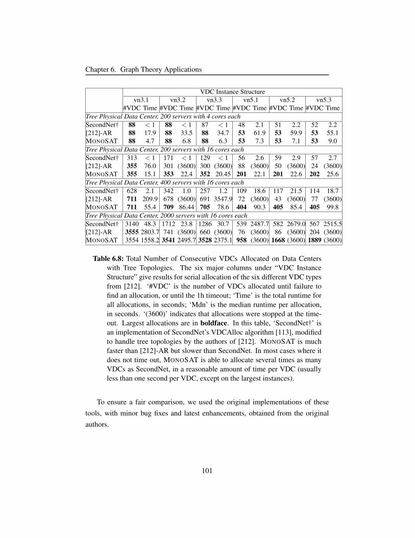
Chapter 6. Graph Theory Applications
VDC Instance Structurevn3.1 vn3.2 vn3.3 vn5.1 vn5.2 vn5.3
#VDC Time #VDC Time #VDC Time #VDC Time #VDC Time #VDC TimeTree Physical Data Center, 200 servers with 4 cores eachSecondNet† 88 < 1 88 < 1 87 < 1 48 2.1 51 2.2 52 2.2[212]-AR 88 17.9 88 33.5 88 34.7 53 61.9 53 59.9 53 55.1MONOSAT 88 4.7 88 6.8 88 6.3 53 7.3 53 7.1 53 9.0Tree Physical Data Center, 200 servers with 16 cores eachSecondNet† 313 < 1 171 < 1 129 < 1 56 2.6 59 2.9 57 2.7[212]-AR 355 76.0 301 (3600) 300 (3600) 88 (3600) 50 (3600) 24 (3600)MONOSAT 355 15.1 353 22.4 352 20.45 201 22.1 201 22.6 202 25.6Tree Physical Data Center, 400 servers with 16 cores eachSecondNet† 628 2.1 342 1.0 257 1.2 109 18.6 117 21.5 114 18.7[212]-AR 711 209.9 678 (3600) 691 3547.9 72 (3600) 43 (3600) 77 (3600)MONOSAT 711 55.4 709 86.44 705 78.6 404 90.3 405 85.4 405 99.8Tree Physical Data Center, 2000 servers with 16 cores eachSecondNet† 3140 48.3 1712 23.8 1286 30.7 539 2487.7 582 2679.0 567 2515.5[212]-AR 3555 2803.7 741 (3600) 660 (3600) 76 (3600) 86 (3600) 204 (3600)MONOSAT 3554 1558.2 3541 2495.7 3528 2375.1 958 (3600) 1668 (3600) 1889 (3600)
Table 6.8: Total Number of Consecutive VDCs Allocated on Data Centerswith Tree Topologies. The six major columns under “VDC InstanceStructure” give results for serial allocation of the six different VDC typesfrom [212]. ‘#VDC’ is the number of VDCs allocated until failure tofind an allocation, or until the 1h timeout; ‘Time’ is the total runtime forall allocations, in seconds; ‘Mdn’ is the median runtime per allocation,in seconds. ‘(3600)’ indicates that allocations were stopped at the time-out. Largest allocations are in boldface. In this table, ‘SecondNet†’ isan implementation of SecondNet’s VDCAlloc algorithm [113], modifiedto handle tree topologies by the authors of [212]. MONOSAT is muchfaster than [212]-AR but slower than SecondNet. In most cases where itdoes not time out, MONOSAT is able to allocate several times as manyVDCs as SecondNet, in a reasonable amount of time per VDC (usuallyless than one second per VDC, except on the largest instances).
To ensure a fair comparison, we used the original implementations of these
tools, with minor bug fixes and latest enhancements, obtained from the original
authors.
101
Chapter 6. Graph Theory Applications
Comparison on Trees from [212] Our first experiment reproduces and extends
an experiment from [212], in which a series of identically structured VDCs are
allocated one-by-one to tree-structured data centers until the solver is unable to
make further allocations (or a timeout of 1 CPU hour is reached). We obtained the
original implementation Z3-AR from the authors for this experiment, along with a
version of SecondNet they implemented with support for the tree-structured data
centers considered here. In this experiment, the VDCs being allocated always have
identical structure; this is a limitation introduced here for compatibility with the
solvers from [212]. In our subsequent experiments, below, we will consider more
realistic allocation scenarios. Except where noted, all experiments were conducted
on a 2.66GHz (12Mb L3 cache) Intel x5650 processor, running Ubuntu 12.04, and
limited to 16GB RAM.
We started with the 200-server/4-cores-per-server physical data center
from [212], but then considered larger versions of the original benchmark to study
performance scaling. The larger data centers are also more representative of current
data centers, using 16-core servers rather than the 4-core servers from the original
paper.
Table 6.8 summarizes our results. SecondNet, being heuristic and incomplete,
is much faster than MONOSAT, but MONOSAT is much faster and more scalable
than Z3-AR. Importantly, we see that MONOSAT is able to scale to thousands
of servers, with typical per-instance allocation times of a few seconds or less per
VDC. Furthermore, on these tree-structured data centers, MONOSAT is typically
able to allocate two or even three times as many VDCs as SecondNet onto the same
infrastructure.
Comparison on BCube and FatTree from [113] The second experiment we con-
ducted is a direct comparison against the original SecondNet implementation, with
the latest updates and bug fixes, obtained from its original authors [113] (this is also
the version of SecondNet we use for all subsequent comparisons in this section).
Note that the implementation of Z3-generic, and both the theory and implementa-
tion of Z3-AR, are restricted to tree topologies, so they could not be included in
these experiments.
The SecondNet benchmark instances are extremely large — in one case ex-
102

Chapter 6. Graph Theory Applications
VDC Instance Structurevn3.1 vn3.2 vn3.3 vn5.1 vn5.2 vn5.3
#VDCTime (s)#VDC Time #VDC Time #VDC Time #VDC Time #VDC TimeFatTree Physical Data Center, 432 servers with 16 cores eachSecondNet 624 < 0.1 360 < 0.1 252 < 0.1 132 < 0.1 132 < 0.1 120 < 0.1MONOSAT 768 148.3 762 257.9 760 247.1 448 317.3 438 315.9 436 323.26BCube Physical Data Center, 512 Servers with 16 cores eachSecondNet 833 < 0.1 486 < 0.1 386 < 0.1 157 < 0.1 195 < 0.1 144 < 0.1MONOSAT 909 201.0 881 347.3 869 310.4 473 502.7 440 423.3 460 412.8FatTree Physical Data Center, 1024 servers with 16 cores eachSecondNet 1520 < 0.1 848 < 0.1 608 < 0.1 272 < 0.1 288 < 0.1 278 < 0.1MONOSAT 1820 787.6 1812 1435.2 1806 1437.5 1064 1941.5 1031 1925.2 963 (3600)BCube Data Center, 1000 Servers with 16 cores eachSecondNet 1774 < 0.1 1559 1.4 1188 2.0 302 < 0.1 356 < 0.1 293 < 0.1MONOSAT 1775 746.6 1713 1350.4 1677 1513.8 938 1741.8 884 1747.1 912 1697.0
Table 6.9: Total Number of Consecutive VDCs Allocated on Data Centerswith FatTree and BCube Topologies. Table labels are the same as in Ta-ble 6.8, but in this table, ‘SecondNet’ refers to the original implementa-tion. As before, SecondNet is much faster, but MONOSAT scales well upto hundreds of servers, typically allocating VDCs in less than a second.And in most cases, MONOSAT allocated many more VDCs to the samephysical data center. (An interesting exception is the lower-left corner.Although MONOSAT is complete for any specific allocation, it is allo-cating VDCs one-at-a-time in an online manner, as do other tools, so theoverall allocation could end up being suboptimal.)
ceeding 100 000 servers — but also extremely easy to allocate: the available band-
width per link is typically ≥ 50× the requested communication bandwidths in the
VDC, so with only 16 cores per server, the bandwidth constraints are mostly ir-
relevant. For such easy allocations, the fast, incomplete approach that Second-
Net uses is the better solution. Accordingly, we scaled the SecondNet instances
down to 432–1024 servers, a realistic size for many real-world data centers. For
these experiments, we generated sets of 10 VDCs each of several sizes (6, 9, 12
and 15 VMs), following the methodology described in [212]. These VDCs have
proportionally greater bandwidth requirements than those originally considered by
SecondNet, requiring 5–10% of the smallest link-level capacities. The resulting
VDC instances are large enough to be representative of many real-world use cases,
103
Chapter 6. Graph Theory Applications
while also exhibiting non-trivial bandwidth constraints. For each of these sets of
VDCs, we then repeatedly allocate instances (in random order) until the data center
is saturated.
Table 6.9 shows allocations made by SecondNet and MONOSAT on two data
centers, one with a BCube topology with 512 servers, and one with a FatTree topol-
ogy with 432 servers. As in our previous experiment, SecondNet is much faster
than MONOSAT, but MONOSAT is fast enough to be practical for data centers
with hundreds of servers, with typical allocation times of a few seconds per VDC
(however, in a minority of cases, MONOSAT did require tens or even hundreds of
seconds for individual allocations). In many cases, MONOSAT was able to allocate
more than twice as many VDCs as SecondNet on these data centers — a substantial
improvement in data center utilization.
Comparison on commercial networks The above comparisons consider how
MONOSAT compares to existing VDC allocation tools on several artificial (but
representative) network topologies from the VDC literature. To address the ques-
tion of whether there are actual real-world VDC applications where MONOSAT
performs not only better than existing tools, but is also fast enough to be used in
practice, we also considered a deployment of a standard Hadoop virtual cluster,
on a set of actual data center topologies. We collaborated with the private cloud
provider ZeroStack [215] to devise an optimal virtual Hadoop cluster to run Tera-
sort [60]. Each Hadoop virtual network consists of a single master VM connected
to 3–11 slave VMs. We consider 5 different sizes of VMs, ranging from 1 CPU and
1GB RAM, to 8 CPUs and 16GB of RAM; for our experiments, the slave VMs are
selected randomly from this set, with the master VM selected randomly but always
at least as large as the largest slave VM. The Hadoop master has tree connectivity
with all slaves, with either a 1 or 2 Gbps network link between the master and each
slave.
The physical data center topology was provided by another company, which
requested to remain anonymous. This company uses a private cloud deployed
across four data centers in two geographic availability zones (AZs): us-west and
us-middle. Each data center contains between 280 and 1200 servers, spread across
1 to 4 clusters with 14 and 40 racks. Each server has 16 cores, 32 GB RAM,
104
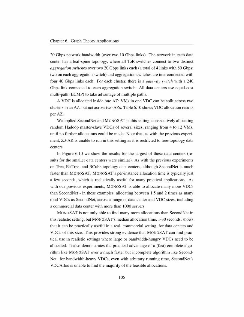
Chapter 6. Graph Theory Applications
20 Gbps network bandwidth (over two 10 Gbps links). The network in each data
center has a leaf-spine topology, where all ToR switches connect to two distinct
aggregation switches over two 20 Gbps links each (a total of 4 links with 80 Gbps;
two on each aggregation switch) and aggregation switches are interconnected with
four 40 Gbps links each. For each cluster, there is a gateway switch with a 240
Gbps link connected to each aggregation switch. All data centers use equal-cost
multi-path (ECMP) to take advantage of multiple paths.
A VDC is allocated inside one AZ: VMs in one VDC can be split across two
clusters in an AZ, but not across two AZs. Table 6.10 shows VDC allocation results
per AZ.
We applied SecondNet and MONOSAT in this setting, consecutively allocating
random Hadoop master-slave VDCs of several sizes, ranging from 4 to 12 VMs,
until no further allocations could be made. Note that, as with the previous experi-
ment, Z3-AR is unable to run in this setting as it is restricted to tree-topology data
centers.
In Figure 6.10 we show the results for the largest of these data centers (re-
sults for the smaller data centers were similar). As with the previous experiments
on Tree, FatTree, and BCube topology data centers, although SecondNet is much
faster than MONOSAT, MONOSAT’s per-instance allocation time is typically just
a few seconds, which is realistically useful for many practical applications. As
with our previous experiments, MONOSAT is able to allocate many more VDCs
than SecondNet - in these examples, allocating between 1.5 and 2 times as many
total VDCs as SecondNet, across a range of data center and VDC sizes, including
a commercial data center with more than 1000 servers.
MONOSAT is not only able to find many more allocations than SecondNet in
this realistic setting, but MONOSAT’s median allocation time, 1-30 seconds, shows
that it can be practically useful in a real, commercial setting, for data centers and
VDCs of this size. This provides strong evidence that MONOSAT can find prac-
tical use in realistic settings where large or bandwidth-hungry VDCs need to be
allocated. It also demonstrates the practical advantage of a (fast) complete algo-
rithm like MONOSAT over a much faster but incomplete algorithm like Second-
Net: for bandwidth-heavy VDCs, even with arbitrary running time, SecondNet’s
VDCAlloc is unable to find the majority of the feasible allocations.
105
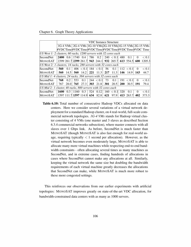
Chapter 6. Graph Theory Applications
VDC Instance Structure1G-4 VMs 2G-4 VMs 1G-10 VMs2G-10 VMs1G-15 VMs 2G-15 VMs
#VDCTime #VDCTime #VDCTime #VDCTime #VDCTime #VDC TimeUS West 1: 2 clusters, 60 racks, 1200 servers with 32 cores eachSecondNet 2400 0.6 1740 0.4 786 0.2 240 < 0.1 480 0.1 0 < 0.1MONOSAT 2399 261.7 2399 261.7 943 244.1 932 265.7 613 554.5 600 1205.3US West 2: 1 clusters, 14 racks, 280 servers with 32 cores eachSecondNet 560 0.1 406 < 0.1 184 < 0.1 56 0.1 112 < 0.1 0 < 0.1MONOSAT 560 14.5 560 14.2 221 11.3 217 11.3 146 14.9 143 44.7US Mid 1: 4 clusters, 24 racks, 384 servers with 32 cores eachSecondNet 768 0.2 553 0.1 244 < 0.1 73 0.1 191 < 0.1 0 < 0.1MONOSAT 767 28.0 765 27.3 303 21.8 301 20.5 200 30.5 191 79.4US Mid 2: 1 cluster, 40 racks, 800 servers with 32 cores eachSecondNet 1600 0.3 1160 0.3 524 0.12 160 < 0.1 320 0.1 0 < 0.1MONOSAT 1597 111.7 1597 114.9 634 82.8 621 97.9 413 263.7 402 373.3
Table 6.10: Total number of consecutive Hadoop VDCs allocated on datacenters. Here we consider several variations of a virtual network de-ployment for a standard Hadoop cluster, on 4 real-world, full-scale com-mercial network topologies. 1G-4 VMs stands for Hadoop virtual clus-ter consisting of 4 VMs (one master and 3 slaves as described Section6.3.4 commercial networks subsection), where master connects with allslaves over 1 Gbps link. As before, SecondNet is much faster thanMONOSAT (though MONOSAT is also fast enough for real-world us-age, requiring typically < 1 second per allocation). However, as thevirtual network becomes even moderately large, MONOSAT is able toallocate many more virtual machines while respecting end-to-end band-width constraints - often allocating several times as many machines asSecondNet, and in extreme cases, finding hundreds of allocations incases where SecondNet cannot make any allocations at all. Similarly,keeping the virtual network the same size but doubling the bandwidthrequirements of each virtual machine greatly decreases the allocationsthat SecondNet can make, while MONOSAT is much more robust tothese more congested settings.
This reinforces our observations from our earlier experiments with artificial
topologies: MONOSAT improves greatly on state-of-the-art VDC allocation, for
bandwidth-constrained data centers with as many as 1000 servers.
106
Chapter 6. Graph Theory Applications
6.4 ConclusionIn this chapter, we have presented comprehensive experimental results from three
diverse fields: procedural content generation, circuit layout, and data center allo-
cation. The experiments demonstrate that our graph theory, as implemented in the
SMT solver MONOSAT using the techniques described in Chapter 4, can extend
the state-of-the-art. Our results in particular highlight the scalability and effec-
tiveness of our support for maximum flow predicates (which are key to the circuit
layout and data center allocation encodings).
At the same time, these experiments also give a picture of some of the cases
where MONOSAT does not perform as well as other approaches. For example, we
saw that for reachability constraints, there are cases where MONOSAT is greatly
more scalable, and also cases where it is greatly less scalable, than the ASP solver
CLASP.
However, while there do exist cases where MONOSAT’s graph theory may
not outperform existing approaches, we have also shown that in many important
cases — and across diverse fields — MONOSAT’s graph theory does in fact attain
state-of-the-art performance that greatly improves upon existing SAT, SMT, or ASP
solvers.
107

Chapter 7
Monotonic Theory of Geometry
The next monotonic theory that we consider is a departure from the other theories
we have explored. This is a theory of predicates concerning the convex hulls of
finite, symbolic point sets (Figure 7.1). There are many common geometric prop-
erties of the convex hulls of point sets that monotonically increase (or decrease) as
additional points are added to the set. For example, the area covered by the convex
hull of a point set may increase (but cannot decrease) as points are added to the set.
Similarly, given a fixed query point q, adding additional points to the point
set can cause the convex hull of that point set to grow large enough to contain q,
but cannot cause a convex hull that previously contained q to no longer contain
q. Similarly, given the convex hulls of two point sets, adding a point to either set
can cause the two hulls to overlap, but cannot cause overlapping hulls to no longer
overlap.
Many other common geometric properties of point sets are also monotonic (ex-
amples include the minimum distance between two point sets, the geometric span
(i.e., the maximum diameter) of a point set, and the weight of the minimum steiner
tree of a point set), but we restrict our attention to convex hulls in this chapter. Our
current implementation is limited to 2 dimensional point sets; however, it should
be straightforward to generalize our solver to 3 or more dimensions.
We implemented a theory solver supporting several predicates of convex hulls
of finite point sets, using the SMMT framework, in our SMT solver MONO-
SAT (described in Appendix A). Our implementation operates over one or more
108
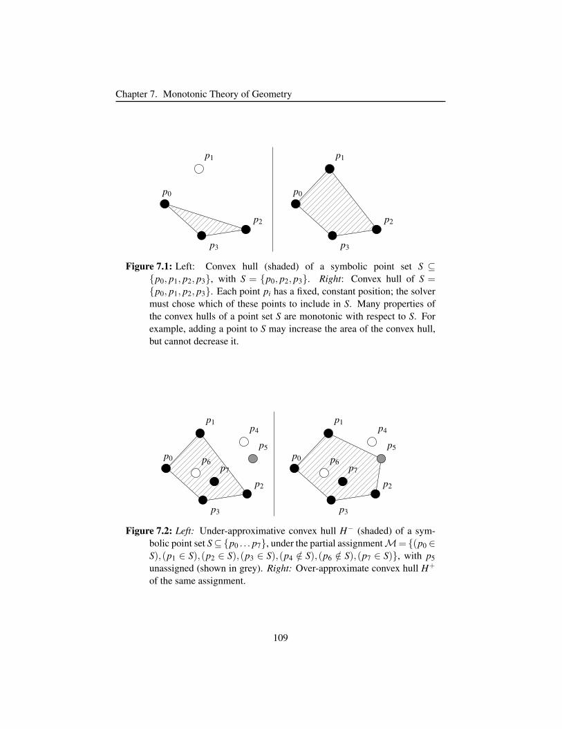
Chapter 7. Monotonic Theory of Geometry
p1
p2
p3
p0
p1
p2
p3
p0
Figure 7.1: Left: Convex hull (shaded) of a symbolic point set S ⊆p0, p1, p2, p3, with S = p0, p2, p3. Right: Convex hull of S =p0, p1, p2, p3. Each point pi has a fixed, constant position; the solvermust chose which of these points to include in S. Many properties ofthe convex hulls of a point set S are monotonic with respect to S. Forexample, adding a point to S may increase the area of the convex hull,but cannot decrease it.
p7p6
p4
p5
p1
p2
p3
p0 p6
p4
p5
p7
p1
p2
p3
p0
Figure 7.2: Left: Under-approximative convex hull H− (shaded) of a sym-bolic point set S⊆p0 . . . p7, under the partial assignmentM= (p0 ∈S),(p1 ∈ S),(p2 ∈ S),(p3 ∈ S),(p4 /∈ S),(p6 /∈ S),(p7 ∈ S), with p5unassigned (shown in grey). Right: Over-approximate convex hull H+
of the same assignment.
109
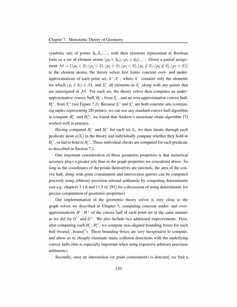
Chapter 7. Monotonic Theory of Geometry
symbolic sets of points S0,S1, . . ., with their elements represented in Boolean
form as a set of element atoms (p0 ∈ S0),(p1 ∈ S0), . . .. Given a partial assign-
ment M = (p0 ∈ S),(p1 ∈ S),(p2 ∈ S),(p3 ∈ S),(p4 /∈ S),(p6 /∈ S),(p7 ∈ S)to the element atoms, the theory solver first forms concrete over- and under-
approximations of each point set, S+,S−, where S− contains only the elements
for which (pi ∈ Si) ∈M, and S+i all elements in S−i along with any points that
are unassigned in M. For each set, the theory solver then computes an under-
approximative convex hull, H−i , from S−i , and an over-approximative convex hull,
H+i , from S+i (see Figure 7.2). Because S−i and S+i are both concrete sets (contain-
ing tuples representing 2D points), we can use any standard convex hull algorithm
to compute H−i and H+i ; we found that Andrew’s monotone chain algorithm [7]
worked well in practice.
Having computed H−i and H+i for each set Si, we then iterate through each
predicate atom p(Si) in the theory and individually compute whether they hold in
H−i , or fail to hold in H+i . These individual checks are computed for each predicate
as described in Section 7.1.
One important consideration of these geometric properties is that numerical
accuracy plays a greater role than in the graph properties we considered above. So
long as the coordinates of the points themselves are rationals, the area of the con-
vex hull, along with point containment and intersection queries can be computed
precisely using arbitrary precision rational arithmetic by computing determinants
(see e.g. chapters 3.1.6 and 11.5 of [91] for a discussion of using determinants for
precise computation of geometric properties).
Our implementation of the geometric theory solver is very close to the
graph solver we described in Chapter 5, computing concrete under- and over-
approximations H−,H+ of the convex hull of each point set in the same manner
as we did for G− and G+. We also include two additional improvements. First,
after computing each H−i ,H+i , we compute axis-aligned bounding boxes for each
hull (bound−i ,bound+i ). These bounding boxes are very inexpensive to compute,
and allow us to cheaply eliminate many collision detections with the underlying
convex hulls (this is especially important when using expensive arbitrary precision
arithmetic).
Secondly, once an intersection (or point containment) is detected, we find a
110
Chapter 7. Monotonic Theory of Geometry
small (but not necessarily minimal) set of points which are sufficient to produce that
collision. For example, when a point is found to be contained in a convex hull, we
can find three points from that hull that together form a triangle that contains that
point. So long as the points composing that triangle remain in the hull, even if other
points are removed from the hull the point will remain contained. These points
can typically be arranged to be computed as a side effect of collision detection,
and their presence in S− of S+ can be checked very cheaply, allowing us to skip
many future collision checks while those points remain in the relevant set. This
is particularly useful for the geometric properties we consider here, as a) a fixed,
small number of points typically constitute a proof of containment (usually 2, 3 or
4), in contrast to potentially very long paths in the graph theory solver of Chapter
5, and b) the geometric properties we are computing may be much more expensive
than the graph properties being computed in the previous section.
Many techniques exist for speeding up the computation of dynamic geometric
properties, especially with regards to collision detection, and we have only imple-
mented the most basic of these (bounding boxes); a more efficient implementation
could make use of more efficient data structures (such as hierarchical bounding
volumes or trapezoidal maps [69]) to greatly speed up or obviate many of the com-
putations in our solver. As before, because these computations are performed on
the concrete under- and over-approximation point sets, standard algorithms or off-
the-shelf collision detection libraries may be used.
7.1 Geometric Predicates of Convex HullsIn this section, we describe the predicates of convex hulls supported by our geom-
etry theory (each of which is a finite, monotonic predicate). For each predicate,
we describe the algorithms used to check the predicates on H− and H+ (as com-
puted above), and to perform conflict analysis when a conflict is detected by theory
propagation.
7.1.1 Areas of Convex Hulls
Given a set of points S, the area of the convex hull of that set of points (shaded
area of Figure 7.1) can increase as more points are added to S, but cannot decrease.
111
Chapter 7. Monotonic Theory of Geometry
This predicate allows us to constrain the area of the convex hull of a point set. In
principle, this predicate could also be set up as a monotonic function (returning the
area of the hull as a rational-value), however as our implementation does not yet
support linear arithmetic, we will treat the area constraints as predicates comparing
the area to fixed, constant values (expressed as arbitrary precision rationals).
Monotonic Predicate: hullArea≥x(S), hullArea>x(S), with S a finite set S ⊆ S′,
true iff the convex hull of the points in S has an area ≥ (resp. >) than x
(where x is a constant). This predicate is positive monotonic with respect to
the set S.
Algorithm: Initially, compute area(bound−),area(bound+). If area(bound−) >
x, compute area(H−); if area(bound+) < x, compute area(H+). The areas
can be computed explicitly, using arbitrary precision rational arithmetic.
Conflict set for hullArea≥x(S): The area of H− is greater or equal to x. Let
p0, p1, . . . be the points of S− that form the vertices of the under-approximate
hull H− (e.g., points p0, p1, p2, p3 in Figure 7.2), with area(H−) ≥ x. Then
at least one of the points must be disabled for the area of the hull to decrease
below x. The conflict set is (p0 ∈ S),(p1 ∈ S), . . . ,¬hullArea≥x(S).
Conflict set for ¬hullArea≥x(S): The area of H+ is less than x; then at least one
point pi /∈ S+ that is not contained in H+ must be added to the point set
to increase the area of H+ (e.g., only point p4 in Figure 7.2). Let points
p0, p1, . . . be the points of S′ not contained in H+. The conflict set is
(p0 /∈ S+),(p1 /∈ S+), . . . ,hullArea≥x(S), where p0, p1, . . . are the (pos-
sibly empty) set of points pi /∈ S+.
7.1.2 Point Containment for Convex Hulls
Given a set of points S, and a fixed point q (Figure 7.3), adding a point to S can
cause the convex hull of S to grow to contain p, but cannot cause a convex hull that
previously contained q to no longer contain q.
Note that this predicate is monotonic with respect to the set of elements in S,
but that it is not monotonic with respect to translating the position of the point q
112

Chapter 7. Monotonic Theory of Geometry
q
p1
p2
p3
p0 q
p1
p2
p3
p0
Figure 7.3: Left: The convex hull (shaded) of a symbolic point set S ⊆p0, p1, p2, p3, along with a query point q. Right: The same as theleft, but with point p1 added to set S. After adding this point, the convexhull of S contains point q.
(which is why q must be a constant). The points that can be contained in S, along
with the query point q, each have constant (2D) positions.
There are a few different reasonable definitions of point containment (all mono-
tonic), depending on whether the convex hull is treated as a closed set (including
both the area inside the hull and also the edges of the hull) or an open set (only the
interior of the hull is included). We consider the closed variant here.
Monotonic Predicate: hullContainsq(S), true iff the convex hull of the 2D points
in S contains the (fixed point) q.
Algorithm: First, check whether q is contained in the under-approximative bound-
ing box bound−. If it is, then check if q is contained in H−. We use the
PNPOLY [95] point inclusion test to perform this check, using arbitrary
precision rational arithmetic, which takes time linear in the number of ver-
tices of H−. In the same way, only if q is contained in bound+, check if q is
contained in H+ using PNPOLY.
Conflict set for hullContainsq(S): Convex hull H− contains p. Let p0, p1, p2 be
three points from H− that form a triangle containing p (such a triangle must
exist, as H− contains p, and we can triangulate H−, so one of those trian-
gles must contain p; this follows from Carathodory’s theorem for convex
hulls [51]). So long as those three points are enabled in S, H− must contain
113

Chapter 7. Monotonic Theory of Geometry
r
p1
p2
p3
p0r
p1
p2
p3
p0
Figure 7.4: Left: The convex hull (shaded) of a symbolic point set S ⊆p0, p1, p2, p3, along with a line-segment r. Right: The same as theleft, but with point p1 added to set S. After adding this point, the convexhull of S intersects line-segment r.
them, and as they contain p, p must be contained in H−. The conflict set is
(p0 ∈ S),(p1 ∈ S),(p2 ∈ S),¬hullContainsq(S).
Conflict set for ¬hullContainsq(S): p is outside of H+. If H+ is empty, then the
conflict set is the default monotonic conflict set. Otherwise, we will em-
ploy the separating axis theorem to produce a conflict set. The separating
axis theorem [91] states that given any two convex volumes, either those
volumes intersect, or there exists a separating axis on which the volumes
projections do not overlap. As we gave two non-intersecting convex hulls,
by the separating axis theorem, there exists a separating axis between H+
and p. Let p0, p1, . . . be the (disabled) points of S whose projection onto that
axis is ≥ the projection of p onto that axis1. At least one of those points
must be enabled in S in order for H+ to grow to contain p. The conflict set
is (p0 /∈ S),(p1 /∈ S), . . . ,hullContainsq(S).
114

Chapter 7. Monotonic Theory of Geometry
7.1.3 Line-Segment Intersection for Convex Hulls
Given a set of points S, and a fixed line-segment r (Figure 7.4), adding a point to
S can cause the convex hull of S to intersect r, but cannot cause a convex hull that
previously intersected r to no longer intersect r.
This predicate directly generalizes the previous predicate (point containment),
and we will utilize some of the methods described above in computing it.
Monotonic Predicate: hullIntersectsr(S), true iff the convex hull of the 2D points
in S intersects the (fixed) line-segment r.
Algorithm: First, check whether line-segment r intersects bound−. If it does,
check if r intersects H−. If H− is empty, is a point, or is itself a line-segment,
this is trivial (and can be checked precisely in arbitrary precision arithmetic
by computing cross products following [110]). Otherwise, we check if ei-
ther end-point of r is contained in H−, using PNPOLY as above for point
containment. If neither end-point is contained, we check whether the line-
segment intersects H−, by testing each edge of H− for intersection with r
(as before, by computing cross-products). If r does not intersect the under-
approximation, repeat the above on bound+ and H+.
Conflict set for hullIntersectsr(S): Convex hull H− intersects line-segment r. If
either end-point or r was contained in H−, then proceed as for the point con-
tainment predicate. Otherwise, the line-segment r intersects with at least one
edge (pi, p j) of H−. Conflict set is (pi ∈ S),(p j ∈ S),¬hullIntersectsr(S).
Conflict set for ¬hullIntersectsr(S): r is outside of H+. If H+ is empty, then the
conflict set is the naıve monotonic conflict set. Otherwise, by the separating
axis theorem, there exists a separating axis between H+ and line-segment r.
Let p0, p1, . . . be the (disabled) points of S whose projection onto that axis is
≥ the projection of the nearest endpoint of r onto that axis. At least one of
1We will make use of the separating axis theorem several times in this chapter. The standard pre-sentation of the separating axis theorem involves normalizing the separating axis (which we wouldnot be able to do using rational arithmetic). This normalization is required if one wishes to computethe minimum distance between the projected point sets; however, if we are only interested in com-paring distances (and testing collisions), we can skip the normalization step, allowing the separatingaxis to be found and applied using only precise rational arithmetic.
115
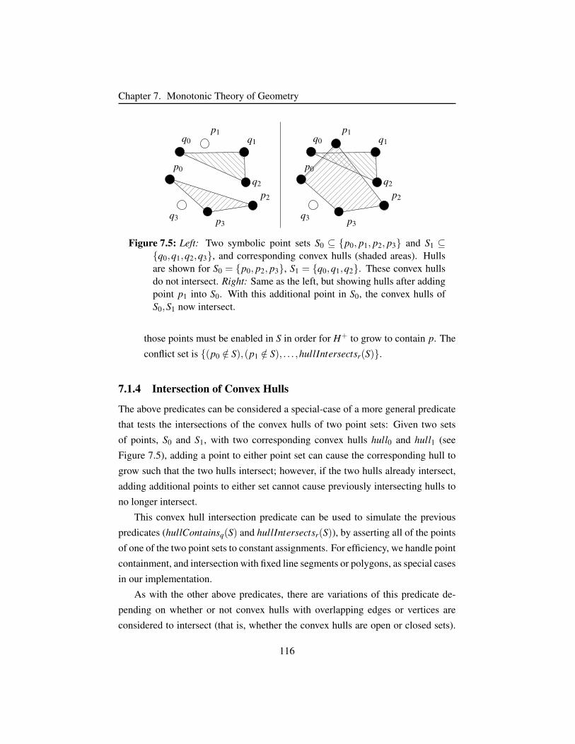
Chapter 7. Monotonic Theory of Geometry
p1
p2
p3
p0
q0 q1
q3
q2
p1
p2
p3
p0
q0 q1
q3
q2
Figure 7.5: Left: Two symbolic point sets S0 ⊆ p0, p1, p2, p3 and S1 ⊆q0,q1,q2,q3, and corresponding convex hulls (shaded areas). Hullsare shown for S0 = p0, p2, p3, S1 = q0,q1,q2. These convex hullsdo not intersect. Right: Same as the left, but showing hulls after addingpoint p1 into S0. With this additional point in S0, the convex hulls ofS0,S1 now intersect.
those points must be enabled in S in order for H+ to grow to contain p. The
conflict set is (p0 /∈ S),(p1 /∈ S), . . . ,hullIntersectsr(S).
7.1.4 Intersection of Convex Hulls
The above predicates can be considered a special-case of a more general predicate
that tests the intersections of the convex hulls of two point sets: Given two sets
of points, S0 and S1, with two corresponding convex hulls hull0 and hull1 (see
Figure 7.5), adding a point to either point set can cause the corresponding hull to
grow such that the two hulls intersect; however, if the two hulls already intersect,
adding additional points to either set cannot cause previously intersecting hulls to
no longer intersect.
This convex hull intersection predicate can be used to simulate the previous
predicates (hullContainsq(S) and hullIntersectsr(S)), by asserting all of the points
of one of the two point sets to constant assignments. For efficiency, we handle point
containment, and intersection with fixed line segments or polygons, as special cases
in our implementation.
As with the other above predicates, there are variations of this predicate de-
pending on whether or not convex hulls with overlapping edges or vertices are
considered to intersect (that is, whether the convex hulls are open or closed sets).
116
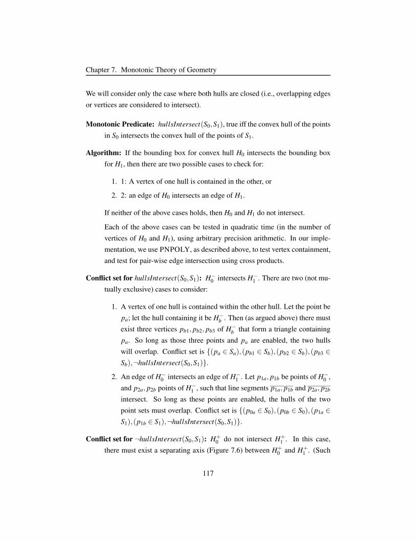
Chapter 7. Monotonic Theory of Geometry
We will consider only the case where both hulls are closed (i.e., overlapping edges
or vertices are considered to intersect).
Monotonic Predicate: hullsIntersect(S0,S1), true iff the convex hull of the points
in S0 intersects the convex hull of the points of S1.
Algorithm: If the bounding box for convex hull H0 intersects the bounding box
for H1, then there are two possible cases to check for:
1. 1: A vertex of one hull is contained in the other, or
2. 2: an edge of H0 intersects an edge of H1.
If neither of the above cases holds, then H0 and H1 do not intersect.
Each of the above cases can be tested in quadratic time (in the number of
vertices of H0 and H1), using arbitrary precision arithmetic. In our imple-
mentation, we use PNPOLY, as described above, to test vertex containment,
and test for pair-wise edge intersection using cross products.
Conflict set for hullsIntersect(S0,S1): H−0 intersects H−1 . There are two (not mu-
tually exclusive) cases to consider:
1. A vertex of one hull is contained within the other hull. Let the point be
pa; let the hull containing it be H−b . Then (as argued above) there must
exist three vertices pb1, pb2, pb3 of H−b that form a triangle containing
pa. So long as those three points and pa are enabled, the two hulls
will overlap. Conflict set is (pa ∈ Sa),(pb1 ∈ Sb),(pb2 ∈ Sb),(pb3 ∈Sb),¬hullsIntersect(S0,S1).
2. An edge of H−0 intersects an edge of H−1 . Let p1a, p1b be points of H−0 ,
and p2a, p2b points of H−1 , such that line segments p1a, p1b and p2a, p2b
intersect. So long as these points are enabled, the hulls of the two
point sets must overlap. Conflict set is (p0a ∈ S0),(p0b ∈ S0),(p1a ∈S1),(p1b ∈ S1),¬hullsIntersect(S0,S1).
Conflict set for ¬hullsIntersect(S0,S1): H+0 do not intersect H+
1 . In this case,
there must exist a separating axis (Figure 7.6) between H+0 and H+
1 . (Such
117
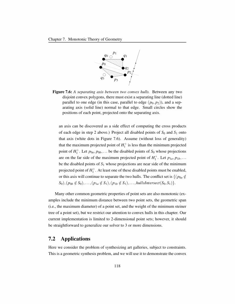
Chapter 7. Monotonic Theory of Geometry
p1
p2
p3
p0
q0 q1
q3
q2
Figure 7.6: A separating axis between two convex hulls. Between any twodisjoint convex polygons, there must exist a separating line (dotted line)parallel to one edge (in this case, parallel to edge (p0, p2)), and a sep-arating axis (solid line) normal to that edge. Small circles show thepositions of each point, projected onto the separating axis.
an axis can be discovered as a side effect of computing the cross products
of each edge in step 2 above.) Project all disabled points of S0 and S1 onto
that axis (white dots in Figure 7.6). Assume (without loss of generality)
that the maximum projected point of H+1 is less than the minimum projected
point of H+1 . Let p0a, p0b, . . . be the disabled points of S0 whose projections
are on the far side of the maximum projected point of H+1 . Let p1a, p1b, . . .
be the disabled points of S1 whose projections are near side of the minimum
projected point of H+1 . At least one of these disabled points must be enabled,
or this axis will continue to separate the two hulls. The conflict set is (p0a /∈S0),(p0b /∈ S0), . . . ,(p1a /∈ S1),(p1b /∈ S1), . . . ,hullsIntersect(S0,S1).
Many other common geometric properties of point sets are also monotonic (ex-
amples include the minimum distance between two point sets, the geometric span
(i.e., the maximum diameter) of a point set, and the weight of the minimum steiner
tree of a point set), but we restrict our attention to convex hulls in this chapter. Our
current implementation is limited to 2-dimensional point sets; however, it should
be straightforward to generalize our solver to 3 or more dimensions.
7.2 ApplicationsHere we consider the problem of synthesizing art galleries, subject to constraints.
This is a geometric synthesis problem, and we will use it to demonstrate the convex
118
Chapter 7. Monotonic Theory of Geometry
hull constraints introduced in this chapter. The Art Gallery problem is a classic NP-
Hard problem [55, 124, 141], in which (in the decision version) one must determine
whether it is possible to surveil the entire floor-plan of a multi-room building with
a limited set of fixed cameras. There are many variations of this problem, and we
will consider a common version in which cameras are restricted to being placed on
vertices, and only every vertex of the room must be seen by a camera (as opposed to
the floor or wall spaces between them). This variant is NP-Complete, by reduction
from the dominating set problem [141].
Here, we introduce a related problem: Art Gallery Synthesis. Art Gallery Syn-
thesis is the problem of designing an ‘art gallery’ (a non-intersecting set of simple
polygons without holes) that can be completely surveilled by at most a given num-
ber of cameras, subject to some other constraints on the allowable design of the
art gallery. The additional constraints may be aesthetic or logistic constraints (for
example, that the area of the floor plan be within a certain range, or that there be
a certain amount of space on the walls). There are many circumstances where one
might want to design a building or room that can be guarded from a small number
of sightlines. Obvious applications include aspects of video game design, but also
prisons and actual art galleries.
Without constraints on the allowable geometry, the solution to the art gallery
synthesis problem is trivial, as any convex polygon can be completely guarded
by a single camera. For this reason, the choice of constraints has a great impact
on the practical difficulty of solving this problem. There are many ways that one
could constrain the art gallery synthesis problem; below, we will describe a set
of constraints that are intended to exhibit the strengths of our convex hull theory
solver, while also producing visually interesting and complex solutions.
We consider the following constrained art gallery synthesis problem: Given a
box containing a fixed set of randomly placed 2-dimensional points, we must find
N non-overlapping convex polygons with vertices selected from those points, such
that a) the area of each polygon is greater than some fixed constant (to prevent lines
or very small slivers from being created), b) the polygons may meet at an edge, but
may not meet at just one vertex (to prevent forming wall segments of infinitesimal
thickness), and c) all vertices of all the polygons, and all 4 corners of the room, can
be seen by a set of at most M cameras (placed at those vertices). Figure 7.7 shows
119

Chapter 7. Monotonic Theory of Geometry
Figure 7.7: Two artificial ‘art galleries’ found by MONOSAT. Cameras arelarge black circles; potential vertices are gray dots. Each convex poly-gon is the convex hull of a subset of those gray dots, selected by thesolver. Notice how the cameras have been placed such that the verticesof all hulls (and the corners of the room) can been seen, some alongvery tight angles, including one vertex completely embedded in threeadjoining polygons. Notice also that some vertices can only be seenfrom one ‘side’, and that some edges cannot be fully observed by cam-eras (as only vertices are required to be observable in this variant of theproblem).
Art Gallery Synthesis MONOSAT Z310 points, 3 polygons, ≤3 cameras 2s 7s20 points, 4 polygons, ≤4 cameras 36s 433s30 points, 5 polygons, ≤5 cameras 187s > 3600s40 points, 6 polygons, ≤6 cameras 645s > 3600s50 points, 7 polygons, ≤7 cameras 3531s > 3600s20 points, 10 polygons, ≤5 cameras 3142s Timeout20 points, 10 polygons, ≤3 cameras 16242s Memout
Table 7.1: Art gallery synthesis results.
two example solutions to these constraints, found by MONOSAT.
In Table 7.1, we compare MONOSAT to an encoding of the above constraints
into the theory of linear arithmetic (as solved by Z3, version 4.3.1). Unfortunately,
the encoding into linear arithmetic is very expensive, using a cubic number of
comparisons to find the points making up the hull of each convex polygon. We
120
Chapter 7. Monotonic Theory of Geometry
describe the encoding in detail in Appendix C.3.
For each instance, we list the number of randomly placed points from which
the vertices of the polygons can be chosen, the number of convex polygons to be
placed, and the maximum number of cameras to be used to observe all the vertices
of the room (with cameras constrained to be placed only on vertices of the placed
polygons, or of the bounding box). These experiments were conducted on an Intel
i7-2600K CPU, at 3.4 GHz (8MB L3 cache), limited to 10 hours of runtime and 16
GB of RAM.
The version of art gallery synthesis that we have considered here is an artificial
one that is likely far removed from a real-world application. Nonetheless, these
examples show that, as compared to a straightforward linear arithmetic encoding,
the geometric predicates supported by MONOSAT can be greatly more scalable,
and show promise for more realistic applications.
121
Chapter 8
Monotonic Theory of CTL
Computation Tree Logic (CTL) synthesis [56] is a long-standing problem with ap-
plications to synthesizing synchronization protocols and concurrent programs. We
show how to formulate CTL model checking as a monotonic theory, enabling us
to use the SMMT framework of Chapter 4 to build a Satisfiability Modulo CTL
solver (implemented as part of our solver MONOSAT, described in Appendix A).
This yields a powerful procedure for CTL synthesis, which is not only faster than
previous techniques from the literature, but also scales to larger and more diffi-
cult formulas. Moreover, our approach is efficient at producing minimal Kripke
structures on common CTL synthesis benchmarks.
Computation tree logic is widely used in the context of model checking, where
a CTL formula specifying a temporal property, such as safety or liveness, is
checked for validity in a program or algorithm (represented by a Kripke structure).
Both the branching time logic CTL and its application to model checking were
first proposed by Clarke and Emerson [56]. In that work, they also introduced
a decision procedure for CTL satisfiability, which they applied to the synthesis
of synchronization skeletons, abstractions of concurrent programs which are no-
toriously difficult to construct manually. Though CTL model checking has found
wide success, there have been fewer advances in the field of CTL synthesis due to
its high complexity.
In CTL synthesis, a system is specified by a CTL formula, and the goal is to
find a model of the formula — a Kripke structure in the form of a transition system
122
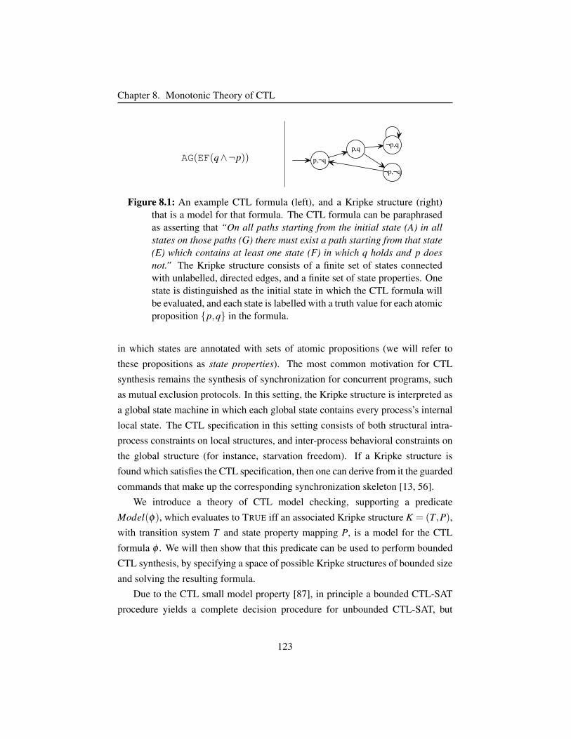
Chapter 8. Monotonic Theory of CTL
AG(EF(q∧¬p)) p,¬q
p,q ¬p,q
¬p,¬q
Figure 8.1: An example CTL formula (left), and a Kripke structure (right)that is a model for that formula. The CTL formula can be paraphrasedas asserting that “On all paths starting from the initial state (A) in allstates on those paths (G) there must exist a path starting from that state(E) which contains at least one state (F) in which q holds and p doesnot.” The Kripke structure consists of a finite set of states connectedwith unlabelled, directed edges, and a finite set of state properties. Onestate is distinguished as the initial state in which the CTL formula willbe evaluated, and each state is labelled with a truth value for each atomicproposition p,q in the formula.
in which states are annotated with sets of atomic propositions (we will refer to
these propositions as state properties). The most common motivation for CTL
synthesis remains the synthesis of synchronization for concurrent programs, such
as mutual exclusion protocols. In this setting, the Kripke structure is interpreted as
a global state machine in which each global state contains every process’s internal
local state. The CTL specification in this setting consists of both structural intra-
process constraints on local structures, and inter-process behavioral constraints on
the global structure (for instance, starvation freedom). If a Kripke structure is
found which satisfies the CTL specification, then one can derive from it the guarded
commands that make up the corresponding synchronization skeleton [13, 56].
We introduce a theory of CTL model checking, supporting a predicate
Model(φ), which evaluates to TRUE iff an associated Kripke structure K = (T,P),
with transition system T and state property mapping P, is a model for the CTL
formula φ . We will then show that this predicate can be used to perform bounded
CTL synthesis, by specifying a space of possible Kripke structures of bounded size
and solving the resulting formula.
Due to the CTL small model property [87], in principle a bounded CTL-SAT
procedure yields a complete decision procedure for unbounded CTL-SAT, but
123
Chapter 8. Monotonic Theory of CTL
in practice, neither bounded approaches, nor classical tableau approaches, have
been scalable enough for completeness to be a practical concern. Rather, our
approach (like similar constraint-solver based techniques for CTL [68, 121] and
LTL [132, 178]) is appropriate for the case where a formula is expected to be satis-
fiable by a Kripke structure with a modest number of states (∼ 100). Nevertheless,
we will show that our approach solves larger and more complex satisfiable CTL
formulas, including ones with a larger numbers of states, much faster than existing
bounded and unbounded synthesis techniques. This makes our approach particu-
larly appropriate for CTL synthesis.
In addition to being more efficient than existing techniques, our approach is
also capable of synthesizing minimal models. As we will discuss below, previous
CTL synthesis approaches were either incapable of finding minimal models [12,
56], or could not do so with comparable scalability to our technique [68, 121].
We begin with a review of related work in Section 8.1. In Sections 8.2 and 8.3,
we show how to apply the SMMT framework to a theory of CTL model checking.
Sections 8.4 and 8.5 explain the most important implementation details and opti-
mizations. In Section 8.6, we provide experimental comparisons to state-of-the-art
techniques showing that our SMMT-approach to CTL synthesis can find solutions
to larger and more complex CTL formulas than comparable techniques in two fam-
ilies of CTL synthesis benchmarks: one derived from mutual exclusion protocols,
and the other derived from readers-writers protocols. Further, our approach does
so without the limitations and extra expert knowledge that previous approaches
require.
8.1 BackgroundThe original 1981 Clarke and Emerson paper introducing CTL synthesis [56] pro-
posed a tableau-based synthesis algorithm, and used this algorithm to construct a
2-process mutex in which each process was guaranteed mutually exclusive access
to the critical section, with starvation freedom.
Subsequently, although there has been steady progress on the general CTL
synthesis problem, the most dramatic gains have been with techniques that are
structurally-constrained, taking a CTL formula along with some additional ‘struc-
124
Chapter 8. Monotonic Theory of CTL
tural’ information about the desired Kripke structure, not specified in CTL, which
is then leveraged to achieve greater scalability than generic CTL synthesis tech-
niques. For example, in 1998, Attie and Emerson [11, 12] introduced a CTL syn-
thesis technique for the case where the Kripke structure is known to be composed
of multiple similar communicating processes. They used this technique to synthe-
size a Kripke structure for a specially constructed 2-process version of the CTL
formula (a ‘pair-program’) in such a way that the produced Kripke structure could
be safely generalized into an N-process solution. This allowed them to produce
a synchronization skeleton for a mutex with 1000 or more processes, far larger
than other techniques. However, while this process scales very well, only certain
CTL properties can be guaranteed to be preserved in the resulting Kripke structure,
and in general the Kripke structure produced this way may be much larger than
the minimal solution to the instance. In particular, EX and AX properties are not
preserved in this process [11].
Additionally, the similar-process synthesis techniques of Attie and Emerson
rely on a generic CTL synthesis method to synthesize these pair-programs. As
such, improvements to the scalability or expressiveness of generic CTL synthesis
methods can be directly applied to improving this pair-program synthesis tech-
nique. Their use of the synthesis method from [56] yields an initially large Kripke
structure that they minimize in an intermediate step. We note that our approach
is particularly suited for synthesizing such pair-programs, not merely for perfor-
mance reasons, but also because it is able to synthesize minimal models directly.
On the topic of finding minimal models, Bustan and Grumberg [49] introduced
a technique for minimizing Kripke structures. However, the minimal models that
our technique produces can in general be smaller than what can be achieved by
starting with a large Kripke structure and subsequently minimizing it. This is be-
cause minimization techniques which are applied on an existing Kripke structure
after its synthesis only yield a structure minimal with respect to equivalent struc-
tures (for some definition of equivalence, e.g. strong or weak bisimulation). This
does not necessarily result in a structure that is the overall minimal model of the
original CTL formula. For this reason, techniques supporting the direct synthesis
of minimal models, such as ours, have an advantage over post-synthesis minimiza-
tion techniques.
125
Chapter 8. Monotonic Theory of CTL
In 2005, Heymans et al. [121] introduced a novel, constraint-based approach
to the general CTL synthesis problem. They created an extension of answer set
programming (ASP) that they called ‘preferential ASP’ and used it to generate a
2-process mutex with the added property of being ‘maximally parallel’, meaning
that each state has a (locally) maximal number of outgoing transitions (without
violating the CTL specification). They argued that this formalized a property that
was implicit in the heuristics of the original 1981 CTL synthesis algorithm, and
that it could result in Kripke structures that were easier to implement as efficient
concurrent programs. As the formulation in their paper does not require additional
structural constraints (though it can support them), it is a general CTL synthesis
method. Furthermore, being a constraint-based method, one can flexibly add struc-
tural or other constraints to guide the synthesis. However, the scalability of their
method was poor.
Subsequently, high performance ASP solvers [104] built on techniques from
Boolean satisfiability solvers were introduced, allowing ASP solvers to solve much
larger and much more difficult ASP formulas. In 2012, De Angelis, Pettorossi, and
Proietti [68] showed that (unextended) ASP solvers could also be used to perform
efficient bounded CTL synthesis, allowing them to use the high performance ASP
solver Clasp [104]. Similar to [12], they introduced a formulation for doing CTL
synthesis via ASP in the case where the desired Kripke structure is composed of
multiple similar processes. Using this approach, they synthesized 2-process and 3-
process mutexes with properties at least as strong as the original CTL specification
from [12]. The work we introduce in this chapter is also a constraint-solver based,
bounded CTL-synthesis technique. However, in Section 8.6, we will show that
our approach scales to larger and more complex specifications than previous work,
while simultaneously avoiding the limitations that prevent those approaches from
finding minimal models.
Our focus in this section has been on this history of the development of CTL
synthesis techniques; for a gentle introduction to CTL semantics (and CTL model
checking), we refer readers to [128].
126
Chapter 8. Monotonic Theory of CTL
8.2 CTL Operators as Monotonic FunctionsA Kripke structure is composed of a finite state transition system (T ) over states S,
and a set of Boolean state properties (P), such that each state property p ∈ P has a
truth value p(s) in every state s ∈ S. One state of the Kripke structure is uniquely
identified as the starting state — below, we will assume that the starting state is
always state s0 unless otherwise stated. A Kripke structure K = (T,P) is said to be
a model of a CTL formula φ if φ evaluates to TRUE in the starting state of K.
The grammar of a CTL formula φ in existential normal form (ENF) is typically
defined recursively as
φ ::= TRUE|a|¬φ |φ ∧φ |EXφ |EGφ |E(φUφ)
with a being a state property.1
However, we will consider a slightly different presentation of CTL that is more
convenient to represent as a theory of CTL model checking. We represent Kripke
structures as a tuple (T,P), with T a transition system and P a set of state property
vectors. As in the graph theory in Chapter 5, we represent the transition system T
as a set of potential transitions T ⊆ S× S, and introduce, for each transition t in
T , a theory atom (t ∈ T ), such that the transition t is enabled in T if and only if
(t ∈ T ) is assigned TRUE. We will also introduce, for each property vector p ∈ P
and each state s ∈ S, a theory atom (p(s)), TRUE iff property p holds in state
s. Together, these transition atoms and property atoms define a bounded Kripke
structure, K = (T,P). P is the set of all state properties in the Kripke structure;
an individual state property p ∈ P can also be represented as a vector of Booleans
A = [p(s1), p(s2), . . . p(sk)] for the k states of the system. This formulation of CTL
model checking as a predicate over a symbolic Kripke structure with a fixed set of
states and a variable set of transitions and property assignments is similar to the
ones introduced in [68, 121].1CTL formulas are also often expressed over a larger set of operators:
AG,EG,AF,EF,AX ,EX ,EU,AU , along with the standard propositional connectives. How-ever, it is sufficient to consider the smaller set of existentially quantified CTL operators EX, EG andEU, along with the propositional operators (¬,∧), and TRUE, which are known to form an adequateset. Any CTL formula can be efficiently converted into a logically equivalent existential normalform (ENF) in terms of these operators, linear in the size of the original formula [147].
127

Chapter 8. Monotonic Theory of CTL
We introduce for each unary CTL operator op an evaluation function op(T,A),
taking as arguments a set of edges specifying the transition system, T , and a 1-
dimensional vector of Booleans, A, of size |S| which indicates the truth value of
property a in each state. Element s of A, written A[s], is interpreted as representing
the truth value of state property a in state s (we assume that the states are uniquely
addressable in such a way that they can be used as indices into this property vector).
For each of the binary operators EU and ∧, we introduce an evaluation function
op(T,A,B), which takes a single transition system as above, and two state property
vectors, A and B, representing the truth value of the arguments of op in each state.
Each evaluation function returns a vector of Booleans C, of size |S|, repre-
senting a fresh state property storing, for each state s, the truth value of evaluat-
ing CTL operator op from initial state s in the Kripke structure K = (T,A) (or
K = (T,A,B) if op takes two arguments). This is a standard interpretation of
CTL (and how explicit-state CTL model checking is often implemented), and we
refer to the literature for common ways to compute each operator (see, e.g., [128]).
We support the following CTL functions (with T a transition system, and
A,B,C vectors of Booleans representing state properties):
• ¬(T,A) 7→C
• ∧(T,A,B) 7→C
• EX(T,A) 7→C
• EG(T,A) 7→C
• EU(T,A,B) 7→C
Notice that there is no operator for specifying state properties; rather, a state
property is specified in the formula directly by passing a vector of state property
atoms as an argument of an operator. For example, consider the following CTL
formula in ENF form:
EG(¬a∧EX(b))
128
Chapter 8. Monotonic Theory of CTL
This formula has two state properties (‘a’ and ‘b’). Given a transition system T ,
this formula can be encoded into our theory of CTL model checking as
EG(T,∧(T,¬(T,a),EX(T,b)))
where a,b are vectors of Booleans representing the truth values of the state prop-
erties a and b at each state in the Kripke structure.2
Before describing our CTL theory solver, we will briefly establish that each
CTL operator as defined above is monotonic. First, we show that the operators
EX(T,A), EG(T,A) or EU(T,A,B) are each monotonic with respect to the state
property vectors A and B. Let solves(φ(T,A)) be a predicate that denotes whether
or not the formula φ holds in state s of the Kripke structure determined by the
vector of Booleans T (transitions) and A (state properties).
Lemma 8.2.1. solves(EX(T,A)), solves(EG(T,A)), and solves(EU(T,A,B)) are
each positive monotonic in both the transition system T and state property A (and
state property B, for EU).
Proof. Take any T , A,B that determine a structure K for which the predicate holds.
Let K′ be a structure determined by some T ′, A′,B′ such that K′ has the same states,
state properties and transitions as K, except for one transition that is enabled in K′
but not in K, or one state property which holds in K′ but not in K. Formally, there
is exactly one argument in either T ′, A′, or B′ that is 0 in T (or A or B respectively)
and 1 in T ′ (or A′ or B′ respectively). Then either (a) one of the states satisfies one
of the atomic propositions in K′, but not in K, or (b) there is a transition in K′, but
not in K.
We assume solves(φ(T,A)) holds (for EU, we assume that solves(φ(T,A,B))
holds). Then, there must exist a witnessing infinite sequence starting from s in
K. If (b), the exact same sequence must exist in K′, since it has a superset of
the transitions in K. Thus we can conclude solves(φ(T ′,A′)) holds (respectively,
2Notice that the transition system T has to be passed as an argument to each function. We canask whether a formula EG(T1,EX(T2,a)), with T1 6= T2, is well-formed? In fact T1 does not need toequal T2 in order to have meaningful semantics, however, if the transition systems are not the same,then the semantics of the formula will not match the expected semantics of CTL. We will assumethat all formulas of interest have the same transition system passed as each argument of the formula.
129

Chapter 8. Monotonic Theory of CTL
solves(φ(T ′,A′,B′)) holds). If (a), then the sequence will only differ in at most
one state, where p holds instead of ¬p (or q instead of ¬q). We note that for each
of the three CTL operators, this sequence will be a witness for K′, if the original
sequence was a witness for K. Thus, solves(φ(T ′,A′)) holds as well (respectively,
solves(φ(T ′,A′,B′)) holds).
It is easy to see that ∧ and ∨ are positive monotonic in the same way, and ¬is negative monotonic. Excluding negation, then, all the CTL operators needed to
express formulas in ENF have positive monotonic solves predicates, while negation
alone has a negative monotonic solves predicate.
Each CTL operator op(T,A) returns a vector of Booleans C, where Ci ←solvei(T,A) (or Ci ← solvei(T,A,B) for the binary operators). It directly follows
that for each op(T,A) 7→C, each entry of Ci is monotonic with respect to arguments
T,A (and also with respect to B, for binary operators).
Finally, we also introduce a predicate Model(A), which takes a Boolean state
property vector A and returns TRUE iff the property A holds in the initial state. For
simplicity, we will further assume (without loss of generality) that the initial state
is always state s0; predicate Model(A) then simply returns the Boolean at index s0
of the vector A: Model(A) 7→ A[s0], and as a result is trivially positive monotonic
with respect to the property state vector A.
8.3 Theory Propagation for CTL Model CheckingAs described in Section 8.2 each CTL operator is monotonic, as is the predicate
Model(A). In Section 4.3, we described an approach to supporting theory propa-
gation for compositions of positive and negative monotonic functions, relying on a
function, approx(φ ,M+A ,M
−A ). In Algorithm 15 we describe our implementation
of Algorithm 8 for the theory of CTL model checking, and in Algorithm 16, we de-
scribe our implementation of approx for the theory of CTL model checking (with
the over- and under-approximative models represented as two Kripke structures,
K+, K−).3 This approximation function in turn calls a function evaluate(op,T,A),
which takes a CTL operator, transition system, and a state property vector and
3Similar recursive algorithms for evaluating CTL formulas on partial Kripke structures, can befound in [43, 115, 142], applied to CTL model checking, rather than CTL synthesis.
130
Chapter 8. Monotonic Theory of CTL
returns a vector of Booleans containing, for each state s in T , the evaluation of
op starting from state s. Our implementation of evaluate is simply the standard
implementation of CTL model checking semantics (e.g., as described in [128]).
While our theory propagation implementation for CTL model checking closely
follows that of Section 4.3, our implementation of conflict analysis differs from
(and improves on) the general case described in Section 4.3. We describe our
implementation of conflict analysis in the next section.
131
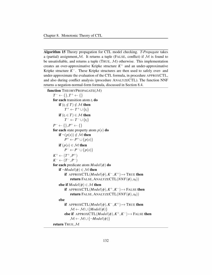
Chapter 8. Monotonic Theory of CTL
Algorithm 15 Theory propagation for CTL model checking. T-Propagate takesa (partial) assignment,M. It returns a tuple (FALSE, conflict) if M is found tobe unsatisfiable, and returns a tuple (TRUE, M) otherwise. This implementationcreates an over-approximative Kripke structure K+ and an under-approximativeKripke structure K−. These Kripke structures are then used to safely over- andunder-approximate the evaluation of the CTL formula, in procedure APPROXCTL,and also during conflict analysis (procedure ANALYZECTL). The function NNFreturns a negation-normal-form formula, discussed in Section 8.4.
function THEORYPROPAGATE(M)T−←,T+←for each transition atom ti do
if (ti /∈ T ) /∈M thenT+← T+∪ti
if (ti ∈ T ) ∈M thenT−← T−∪ti
P−←,P+←for each state property atom p(s) do
if ¬(p(s)) /∈M thenP+← P+∪p(s)
if (p(s) ∈M thenP−← P−∪p(s)
K+← (T+,P+)K−← (T−,P−)for each predicate atom Model(φ) do
if ¬Model(φ) ∈M thenif APPROXCTL(Model(φ),K−,K+) 7→ TRUE then
return FALSE,ANALYZECTL(NNF(φ),s0))
else if Model(φ) ∈M thenif APPROXCTL(Model(φ),K+,K−) 7→ FALSE then
return FALSE,ANALYZECTL(NNF(φ),s0))
elseif APPROXCTL(Model(φ),K−,K+) 7→ TRUE thenM←M∪Model(φ)
else if APPROXCTL(Model(φ),K+,K−) 7→ FALSE thenM←M∪¬Model(φ)
return TRUE,M
132
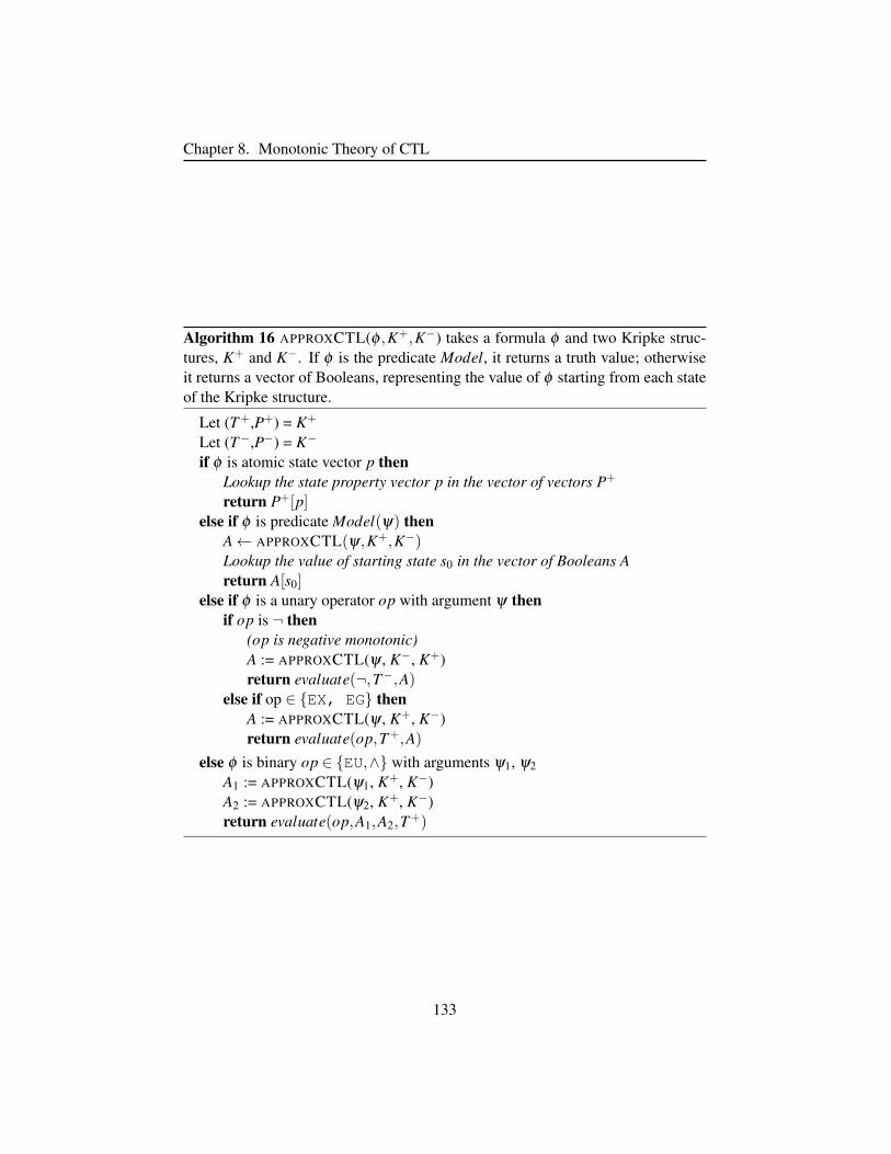
Chapter 8. Monotonic Theory of CTL
Algorithm 16 APPROXCTL(φ ,K+,K−) takes a formula φ and two Kripke struc-tures, K+ and K−. If φ is the predicate Model, it returns a truth value; otherwiseit returns a vector of Booleans, representing the value of φ starting from each stateof the Kripke structure.
Let (T+,P+) = K+
Let (T−,P−) = K−
if φ is atomic state vector p thenLookup the state property vector p in the vector of vectors P+
return P+[p]else if φ is predicate Model(ψ) then
A← APPROXCTL(ψ,K+,K−)Lookup the value of starting state s0 in the vector of Booleans Areturn A[s0]
else if φ is a unary operator op with argument ψ thenif op is ¬ then
(op is negative monotonic)A := APPROXCTL(ψ , K−, K+)return evaluate(¬,T−,A)
else if op ∈ EX, EG thenA := APPROXCTL(ψ , K+, K−)return evaluate(op,T+,A)
else φ is binary op ∈ EU,∧ with arguments ψ1, ψ2A1 := APPROXCTL(ψ1, K+, K−)A2 := APPROXCTL(ψ2, K+, K−)return evaluate(op,A1,A2,T+)
133
Chapter 8. Monotonic Theory of CTL
8.4 Conflict Analysis for the Theory of CTLAbove we described our support for theory propagation for the theory of CTL
model checking, relying on the function composition support described in Section
4.3. Here, we describe our implementation of conflict analysis for the theory of
CTL model checking.
Unlike our theory propagation implementation, which operates on formulas in
existential normal form, to perform conflict analysis we convert the CTL formula
into negation normal form (NNF), pushing any negation operators down to the
innermost terms of the formula. To obtain an adequate set, the formula may now
also include universally quantified CTL operators and Weak Until. In Algorithm
15 above, the function NNF(φ) takes a formula in existential normal form and
returns an equivalent formula in negation normal form. This translation to negation
normal form takes time linear in the size of the input formula; the translation can
be performed once, during preprocessing, and cached for future calls.
Our procedure ANALYZECTL(φ ,s,K+,K−,M) operates recursively on the
NNF formula, handling each CTL operator with a separate case, and returns a con-
flict set of theory literals. In Algorithm 17 below, we show only the cases handling
operators EX ,AX ,EF,AF ; the full algorithm including support for the remaining
cases can be found in Appendix D.4.
134
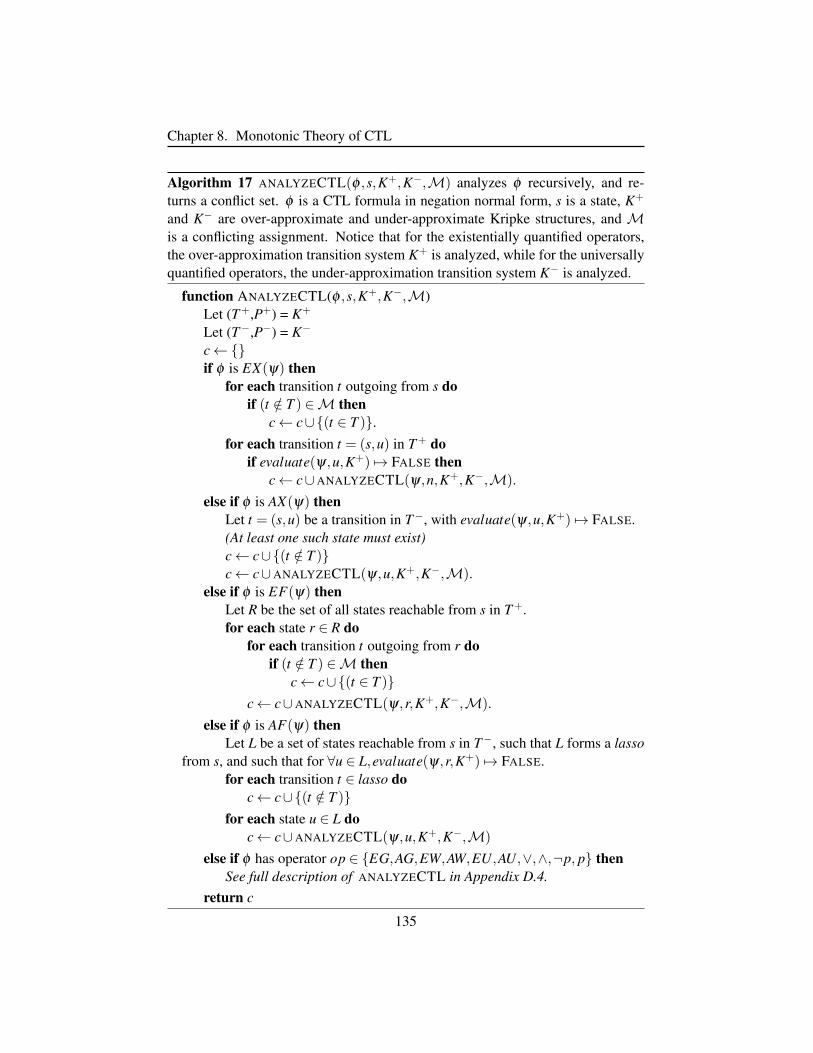
Chapter 8. Monotonic Theory of CTL
Algorithm 17 ANALYZECTL(φ ,s,K+,K−,M) analyzes φ recursively, and re-turns a conflict set. φ is a CTL formula in negation normal form, s is a state, K+
and K− are over-approximate and under-approximate Kripke structures, and Mis a conflicting assignment. Notice that for the existentially quantified operators,the over-approximation transition system K+ is analyzed, while for the universallyquantified operators, the under-approximation transition system K− is analyzed.
function ANALYZECTL(φ ,s,K+,K−,M)Let (T+,P+) = K+
Let (T−,P−) = K−
c←if φ is EX(ψ) then
for each transition t outgoing from s doif (t /∈ T ) ∈M then
c← c∪(t ∈ T ).for each transition t = (s,u) in T+ do
if evaluate(ψ,u,K+) 7→ FALSE thenc← c∪ANALYZECTL(ψ,n,K+,K−,M).
else if φ is AX(ψ) thenLet t = (s,u) be a transition in T−, with evaluate(ψ,u,K+) 7→ FALSE.(At least one such state must exist)c← c∪(t /∈ T )c← c∪ANALYZECTL(ψ,u,K+,K−,M).
else if φ is EF(ψ) thenLet R be the set of all states reachable from s in T+.for each state r ∈ R do
for each transition t outgoing from r doif (t /∈ T ) ∈M then
c← c∪(t ∈ T )c← c∪ANALYZECTL(ψ,r,K+,K−,M).
else if φ is AF(ψ) thenLet L be a set of states reachable from s in T−, such that L forms a lasso
from s, and such that for ∀u ∈ L,evaluate(ψ,r,K+) 7→ FALSE.for each transition t ∈ lasso do
c← c∪(t /∈ T )for each state u ∈ L do
c← c∪ANALYZECTL(ψ,u,K+,K−,M)
else if φ has operator op ∈ EG,AG,EW,AW,EU,AU,∨,∧,¬p, p thenSee full description of ANALYZECTL in Appendix D.4.
return c
135
Chapter 8. Monotonic Theory of CTL
8.5 Implementation and OptimizationsIn Section 8.2, we showed how CTL model checking can be posed as a monotonic
theory. In Sections 8.3 and 8.4, we then described our implementation of the theory
propagation and conflict analysis procedures of a lazy SMT theory solver, follow-
ing the techniques for supporting compositions of positive and negative monotonic
functions and predicates described in Section 4.3. We have also implemented some
additional optimizations which greatly improve the performance of our CTL the-
ory solver. One basic optimization that we implement is pure literal filtering (see,
e.g. [179]): For the case where Model(φ ) is assigned TRUE (resp. FALSE), we
need to check only whether Model(φ) is falsified (resp., made true) during theory
propagation. In all of the instances we will examine in this chapter, Model(φ)
is asserted TRUE in the input formula, and so this optimization greatly simplifies
theory propagation. We describe several further improvements below.
In Section 8.5.1 we describe symmetry breaking constraints, which can greatly
reduce the search space of the solver, and in Section 8.5.2 we show how several
common types of CTL constraints can be cheaply converted into CNF, reducing
the size of the formula the theory solver must handle. Finally, in Section 8.5.3, we
discuss how in the common case of a CTL formula describing multiple commu-
nicating processes, we can (optionally) add support for additional structural con-
straints, similarly to the approach described in [68]. These structural constraints
allow our solver even greater scalability, at the cost of adding more states into the
smallest solution that can be synthesized.4
8.5.1 Symmetry Breaking
Due to the way we expose atomic propositions and transitions to the SAT solver
with theory atoms, the SAT solver may end up exploring large numbers of iso-
morphic Kripke structures. We address this by enforcing extra symmetry-breaking
constraints which prevent the solver from considering (some) redundant configu-
rations of the Kripke structure. Symmetry reduction is especially helpful to prove
instances UNSAT, which aids the search for suitable bounds.4Thus, if structural constraints are used, iteratively decreasing the bound may no longer yield a
minimal structure.
136

Chapter 8. Monotonic Theory of CTL
Let label(si) be the binary representation of the atomic propositions of state si,
and let out(si) be the set of outgoing edges of state si. Let s0 be the initial state.
The following constraint enforces an order on the allowable assignments of state
properties and transitions in the Kripke structure:
∀i, j :[i < j∧ i 6= 0∧ j 6= 0]→[(label(si)≤ label(s j)) ∧
((label(si) = label(s j)
)→(|out(si)| ≤ |out(s j)|
))]8.5.2 Preprocessing
Given a CTL specification φ , we identify certain common sub-expressions which
can be cheaply converted directly into CNF, which is efficiently handled by the
SAT solver at the core of MONOSAT. We do so if φ matches∧
i φi, as is commonly
the case when multiple properties are part of the specification. If φi is purely propo-
sitional, or of the form AGp, with p purely propositional, we eliminate φi from the
formula and convert φi into a logically equivalent CNF expression over the state
property assignment atoms of the theory.5 This requires a linear number of clauses
in the number of states in K. We also convert formulas of the form AGψ , with ψ
containing only propositional logic and at most a single Next-operator (EX or AX).
Both of these are frequent sub-expressions in the CTL formulas that we have seen.
8.5.3 Wildcard Encoding for Concurrent Programs
As will be further explained later, the synthesis problem for synchronization skele-
tons assumes a given number of processes, which each have a local transition sys-
tem. The state transitions in the full Kripke structure then represent the possible
interleavings of executing the local transition system of each process. This local
transition system is normally encoded into the CTL specification.
Both [12] and [68] explored strategies to take advantage of the case where the
local transition systems of these processes are made explicit. The authors of [68]
found they could greatly improve the scalability of their answer-set-programming
5Since AGp only specifies reachable states, the clause is for each state s, a disjunction of p beingsatisfied in s, or s having no enabled incoming transitions. This changes the semantics of CTL forunreachable states, but not for reachable states.
137

Chapter 8. Monotonic Theory of CTL
based CTL synthesis procedure by deriving additional ‘structural’ constraints for
such concurrent processes. As our approach is also constraint-based, we can (op-
tionally) support similar structural constraints. In experiments below, we show that
even though our approach already scales better than existing approaches without
these additional structural constraints, we also benefit from such constraints.
Firstly, we can exclude any global states with state properties that are an illegal
encoding of multiple processes. If the local state of each process is identified by a
unique atomic proposition, then we can enforce that each global state must make
true exactly one of the atomic propositions for each process. For every remaining
combination of state property assignments, excluding those determined to be illegal
above, we add a single state into the Kripke structure, with a pre-determined as-
signment of atomic propositions, such that only the transitions between these states
are free for the SAT solver to assign. This is in contrast to performing synthesis
without structural constraints, in which case all states are completely undetermined
(but typically fewer are required).
Secondly, since we are interested in interleavings of concurrent programs, on
each transition in the global Kripke structure, we enforce that only a single process
may change its local state, and it may change its local state only in a way that is
consistent with its local transition system.
The above two constraints greatly reduce the space of transitions in the global
Kripke structure that are left free for the SAT solver to assign (and completely
eliminate the space of atomic propositions to assign in each state). However these
constraints make our procedure incomplete, since in general more than a single
state with the same atomic propositions (but different behavior) need to be distin-
guished. To allow multiple states with equivalent atomic propositions, we also add
a small number of ‘wildcard’ states into the Kripke structure, whose state proper-
ties and transitions (incoming and outgoing) are not set in advance. In the examples
we consider in this chapter, we have found that a small number of such wildcard
states (between 3 and 20) are sufficient to allow for a Kripke structure that satisfies
the CTL formula, while still greatly restricting the total space of Kripke structures
that must be explored by the SAT solver.
We disable symmetry breaking when using the wildcard encoding, as the wild-
card encoding is incompatible with the constraint in Section 8.5.1.
138
Chapter 8. Monotonic Theory of CTL
8.6 Experimental ResultsThere are few CTL synthesis implementations available for comparison. Indeed,
the original CTL synthesis/model-checking paper [56] presents an implementation
of CTL model checking, but the synthesis examples were simulated by hand. The
only publicly available, unbounded CTL synthesis tool we could find is Prezza’s
open-source CTLSAT tool6, which is a modern implementation of the classic
tableau-based CTL synthesis algorithm [56].
We also compare to De Angelis et al.’s encoding of bounded CTL synthesis
into ASP [68]. De Angelis et al. provide encodings7 specific to the n-process mu-
tual exclusion example, which exploit structural assumptions about the synthesized
model (for example, that it is the composition of n identical processes). We label
this encoding “ASP-structural” in the tables below. For ASP-structural, we have
only the instances originally considered in [68].
To handle the general version of CTL synthesis (without added structural in-
formation), we also created ASP encodings using the methods from De Angelis et
al.’s paper, but without problem-specific structural assumptions and optimizations.
We label those results “ASP-generic”. For both encodings, we use the latest ver-
sion (4.5.4) of Clingo [104], and for each instance we report the best performance
over the included Clasp configurations.8
We compare these tools to two versions of MONOSAT: MONOSAT-structural,
which uses the wildcard optimization presented in Section 8.5.3, and MONOSAT-
generic, without the wildcard optimization.
With the exception of CTLSAT, the tools we consider are bounded synthe-
sis tools, which take as input both a CTL formula and a maximum number of
states. For ASP-structural, the state bounds follow [68]. For the remaining tools,
we selected the state bound manually, by repeatedly testing each tool with different
bounds, and reporting for each tool the smallest bound for which it found a satis-
fying solution. In cases where a tool could not find any satisfying solution within
our time or memory bounds, we report out-of-time or out-of-memory.
6https://github.com/nicolaprezza/CTLSAT7http://www.sci.unich.it/∼deangelis/papers/mutex FI.tar.gz8 These are: “auto”, “crafty”, “frumpy”, “handy”, “jumpy”, “trendy”, and “tweety”.
139
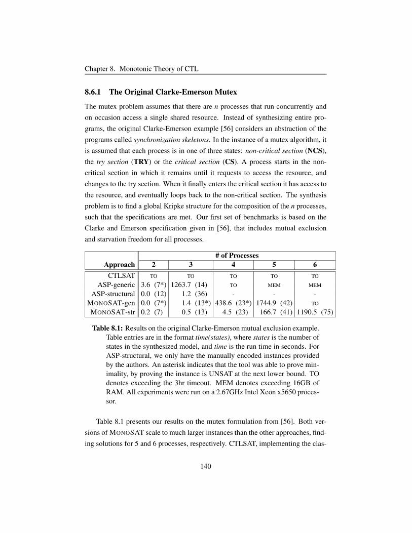
Chapter 8. Monotonic Theory of CTL
8.6.1 The Original Clarke-Emerson Mutex
The mutex problem assumes that there are n processes that run concurrently and
on occasion access a single shared resource. Instead of synthesizing entire pro-
grams, the original Clarke-Emerson example [56] considers an abstraction of the
programs called synchronization skeletons. In the instance of a mutex algorithm, it
is assumed that each process is in one of three states: non-critical section (NCS),
the try section (TRY) or the critical section (CS). A process starts in the non-
critical section in which it remains until it requests to access the resource, and
changes to the try section. When it finally enters the critical section it has access to
the resource, and eventually loops back to the non-critical section. The synthesis
problem is to find a global Kripke structure for the composition of the n processes,
such that the specifications are met. Our first set of benchmarks is based on the
Clarke and Emerson specification given in [56], that includes mutual exclusion
and starvation freedom for all processes.
# of ProcessesApproach 2 3 4 5 6
CTLSAT TO TO TO TO TO
ASP-generic 3.6 (7*) 1263.7 (14) TO MEM MEM
ASP-structural 0.0 (12) 1.2 (36) - - -
MONOSAT-gen 0.0 (7*) 1.4 (13*) 438.6 (23*) 1744.9 (42) TO
MONOSAT-str 0.2 (7) 0.5 (13) 4.5 (23) 166.7 (41) 1190.5 (75)
Table 8.1: Results on the original Clarke-Emerson mutual exclusion example.Table entries are in the format time(states), where states is the number ofstates in the synthesized model, and time is the run time in seconds. ForASP-structural, we only have the manually encoded instances providedby the authors. An asterisk indicates that the tool was able to prove min-imality, by proving the instance is UNSAT at the next lower bound. TOdenotes exceeding the 3hr timeout. MEM denotes exceeding 16GB ofRAM. All experiments were run on a 2.67GHz Intel Xeon x5650 proces-sor.
Table 8.1 presents our results on the mutex formulation from [56]. Both ver-
sions of MONOSAT scale to much larger instances than the other approaches, find-
ing solutions for 5 and 6 processes, respectively. CTLSAT, implementing the clas-
140
Chapter 8. Monotonic Theory of CTL
sical tableau approach, times out on all instances.9 Only the -generic versions
can guarantee minimal solutions, and MONOSAT-generic is able to prove minimal
models for several cases.
As expected, structural constraints greatly improve efficiency for both ASP-
structural and MONOSAT-structural relative to their generic counterparts.
8.6.2 Mutex with Additional Properties
As noted in [121], the original Clarke-Emerson specification permits Kripke struc-
tures that are not maximally parallel, or even practically reasonable. For instance,
our methods synthesize a structure in which one process being in NCS will block
another process in TRY from getting the resource — the only transition such a
global state has is to a state in which both processes are in the TRY section. In
addition to the original formula, we present results for an augmented version in
which we eliminate that solution10 by introducing the “Non-Blocking” property,
which states that a process may always remain in the NCS:
AG (NCSi→ EX NCSi) (NB)
In addition, in the original paper there are structural properties implicit in the
given local transition system, preventing jumping from NCS to CS, or from CS to
TRY. We encode these properties into CTL as “No Jump” properties.
AG (NCSi→ AX ¬CSi) ∧ AG (CSi→ AX ¬TRYi) (NJ)
We also consider two properties from [68]: Bounded Overtaking (BO), which
guarantees that when a process is waiting for the critical section, each other process
can only access the critical section at most once before the first process enters the
9Notably, CTLSAT times out even when synthesizing the original 2-process mutex from [56],which Clarke and Emerson originally synthesized by hand. This may be because in that work, thelocal transition system was specified implicitly in the algorithm, instead of in the CTL specificationas it is here.
10 While the properties that we introduce in this chapter mitigate some of the effects of underspec-ification, we have observed that the formulas of many instances in our benchmarks are not strongenough to guarantee a sensible solution. We are mainly interested in establishing benchmarks forsynthesis performance, which is orthogonal to the task of finding suitable CTL specifications, whichresolve these problems.
141
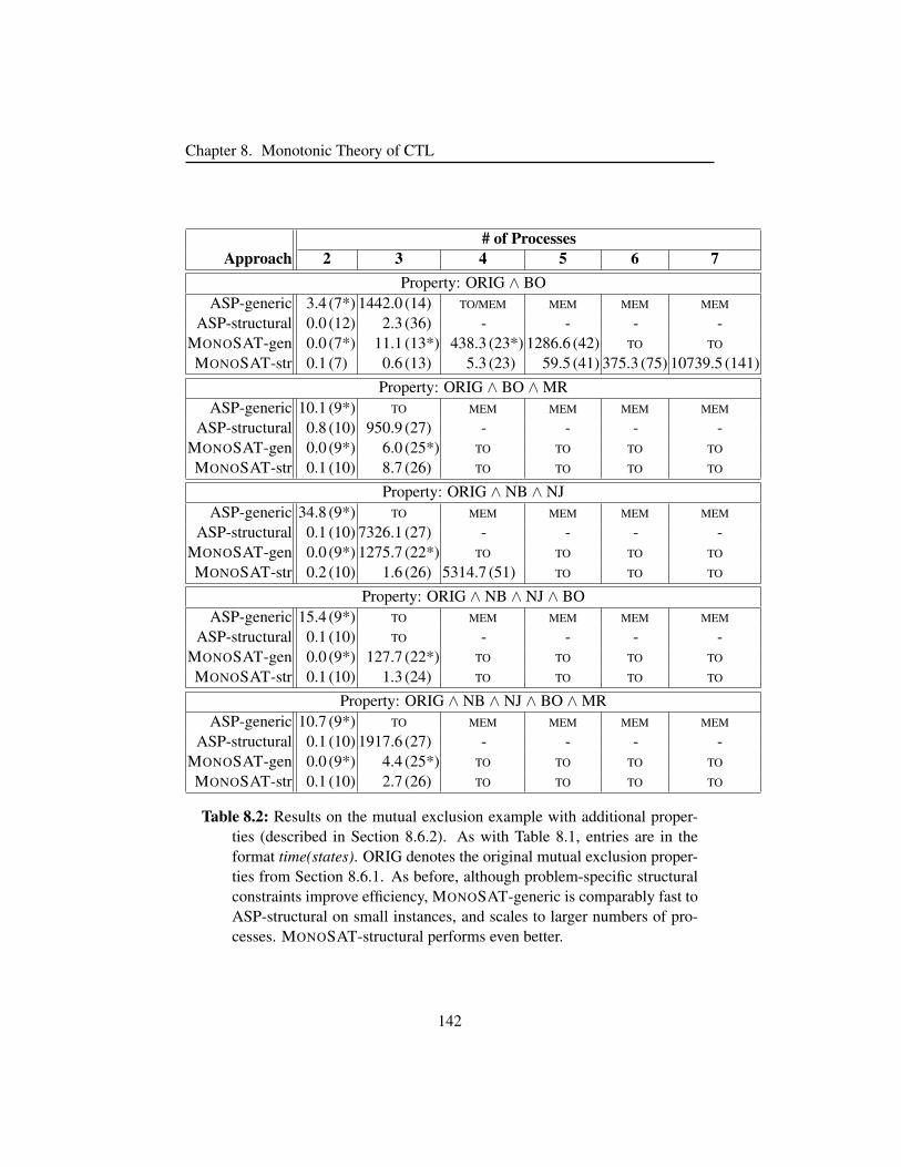
Chapter 8. Monotonic Theory of CTL
# of ProcessesApproach 2 3 4 5 6 7
Property: ORIG ∧ BOASP-generic 3.4 (7*) 1442.0 (14) TO/MEM MEM MEM MEM
ASP-structural 0.0 (12) 2.3 (36) - - - -MONOSAT-gen 0.0 (7*) 11.1 (13*) 438.3 (23*) 1286.6 (42) TO TO
MONOSAT-str 0.1 (7) 0.6 (13) 5.3 (23) 59.5 (41) 375.3 (75) 10739.5 (141)Property: ORIG ∧ BO ∧MR
ASP-generic 10.1 (9*) TO MEM MEM MEM MEM
ASP-structural 0.8 (10) 950.9 (27) - - - -MONOSAT-gen 0.0 (9*) 6.0 (25*) TO TO TO TO
MONOSAT-str 0.1 (10) 8.7 (26) TO TO TO TO
Property: ORIG ∧ NB ∧ NJASP-generic 34.8 (9*) TO MEM MEM MEM MEM
ASP-structural 0.1 (10) 7326.1 (27) - - - -MONOSAT-gen 0.0 (9*) 1275.7 (22*) TO TO TO TO
MONOSAT-str 0.2 (10) 1.6 (26) 5314.7 (51) TO TO TO
Property: ORIG ∧ NB ∧ NJ ∧ BOASP-generic 15.4 (9*) TO MEM MEM MEM MEM
ASP-structural 0.1 (10) TO - - - -MONOSAT-gen 0.0 (9*) 127.7 (22*) TO TO TO TO
MONOSAT-str 0.1 (10) 1.3 (24) TO TO TO TO
Property: ORIG ∧ NB ∧ NJ ∧ BO ∧MRASP-generic 10.7 (9*) TO MEM MEM MEM MEM
ASP-structural 0.1 (10) 1917.6 (27) - - - -MONOSAT-gen 0.0 (9*) 4.4 (25*) TO TO TO TO
MONOSAT-str 0.1 (10) 2.7 (26) TO TO TO TO
Table 8.2: Results on the mutual exclusion example with additional proper-ties (described in Section 8.6.2). As with Table 8.1, entries are in theformat time(states). ORIG denotes the original mutual exclusion proper-ties from Section 8.6.1. As before, although problem-specific structuralconstraints improve efficiency, MONOSAT-generic is comparably fast toASP-structural on small instances, and scales to larger numbers of pro-cesses. MONOSAT-structural performs even better.
142
Chapter 8. Monotonic Theory of CTL
critical section, and Maximal Reactivity (MR), which guarantees that if exactly one
process is waiting for the critical section, then that process can enter the critical
section in the next step.
In Table 8.2, we repeat our experimental procedure from Section 8.6.1, adding
various combinations of additional properties. This provides a richer set of bench-
marks, most of which are harder than the original. As before, the -structural con-
straints greatly improve efficiency, but nevertheless, MONOSAT-generic outper-
forms ASP-structural. MONOSAT-generic is able to prove minimality on several
benchmarks, and on one benchmark, MONOSAT-structural scales to 7 processes.
8.6.3 Readers-Writers
To provide even more benchmarks, we present instances of the related Readers-
Writers problem [63]. Whereas the Mutex problem assumes that all processes
require exclusive access to a resource, the Readers-Writers problem permits some
simultaneous access. Two types of processes are distinguished: writers, which re-
quire exclusive access, and readers, which can share their access with other readers.
This is a typical scenario for concurrent access to shared memory, in which write
permissions and read permissions are to be distinguished. The local states of each
process are as in the Mutex instances.
We use Attie’s [11] CTL specification. We note however that this specification
allows for models which are not maximally parallel, and in particular disallows
concurrent access by two readers. In addition to this original formula, we also
consider one augmented with the Multiple Readers Eventually Critical (MREC)
property. This ensures that there is a way for all readers, if they are in TRY, to
simultaneously enter the critical section, if no writer requests the resource.
AG (∧wi
NCSwi → (∧ri
TRYri → EF∧ri
CSri)) (RW-MREC)
This property turns out not to be strong enough to enforce that concurrent ac-
cess for readers must always be possible. We introduce the following property,
which we call Multiple Readers Critical. It states that if a reader is in TRY, and all
other readers are in CS, it is possible to enter the CS in a next state – as long as all
writers are in NCS, since they have priority access over readers.
143
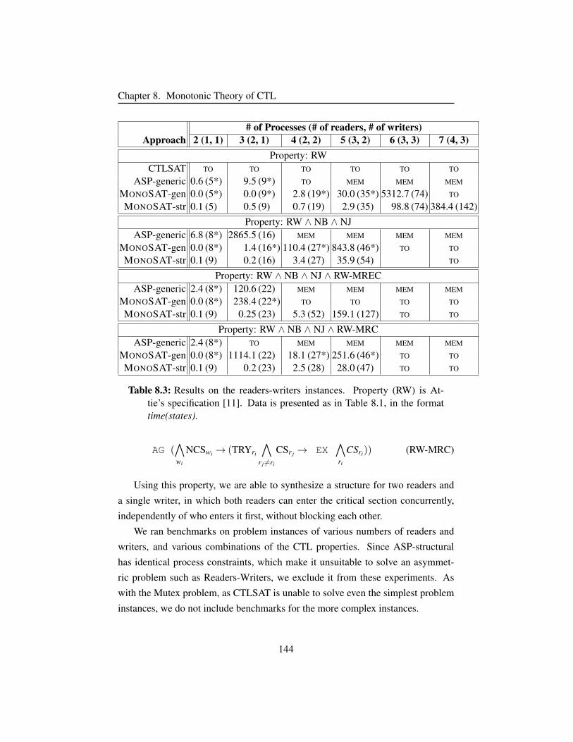
Chapter 8. Monotonic Theory of CTL
# of Processes (# of readers, # of writers)Approach 2 (1, 1) 3 (2, 1) 4 (2, 2) 5 (3, 2) 6 (3, 3) 7 (4, 3)
Property: RWCTLSAT TO TO TO TO TO TO
ASP-generic 0.6 (5*) 9.5 (9*) TO MEM MEM MEM
MONOSAT-gen 0.0 (5*) 0.0 (9*) 2.8 (19*) 30.0 (35*) 5312.7 (74) TO
MONOSAT-str 0.1 (5) 0.5 (9) 0.7 (19) 2.9 (35) 98.8 (74) 384.4 (142)Property: RW ∧ NB ∧ NJ
ASP-generic 6.8 (8*) 2865.5 (16) MEM MEM MEM MEM
MONOSAT-gen 0.0 (8*) 1.4 (16*) 110.4 (27*) 843.8 (46*) TO TO
MONOSAT-str 0.1 (9) 0.2 (16) 3.4 (27) 35.9 (54) TO
Property: RW ∧ NB ∧ NJ ∧ RW-MRECASP-generic 2.4 (8*) 120.6 (22) MEM MEM MEM MEM
MONOSAT-gen 0.0 (8*) 238.4 (22*) TO TO TO TO
MONOSAT-str 0.1 (9) 0.25 (23) 5.3 (52) 159.1 (127) TO TO
Property: RW ∧ NB ∧ NJ ∧ RW-MRCASP-generic 2.4 (8*) TO MEM MEM MEM MEM
MONOSAT-gen 0.0 (8*) 1114.1 (22) 18.1 (27*) 251.6 (46*) TO TO
MONOSAT-str 0.1 (9) 0.2 (23) 2.5 (28) 28.0 (47) TO TO
Table 8.3: Results on the readers-writers instances. Property (RW) is At-tie’s specification [11]. Data is presented as in Table 8.1, in the formattime(states).
AG (∧wi
NCSwi → (TRYri
∧r j 6=ri
CSr j → EX∧ri
CSri)) (RW-MRC)
Using this property, we are able to synthesize a structure for two readers and
a single writer, in which both readers can enter the critical section concurrently,
independently of who enters it first, without blocking each other.
We ran benchmarks on problem instances of various numbers of readers and
writers, and various combinations of the CTL properties. Since ASP-structural
has identical process constraints, which make it unsuitable to solve an asymmet-
ric problem such as Readers-Writers, we exclude it from these experiments. As
with the Mutex problem, as CTLSAT is unable to solve even the simplest problem
instances, we do not include benchmarks for the more complex instances.
144
Chapter 8. Monotonic Theory of CTL
Our experiments on each variation of the Readers-Writer problem are presented
in Table 8.3. We observe that in general, Readers-Writers instances are easier
to solve than Mutex instances with the same number of processes. At the same
time, the additional properties introduced by us restrict the problem further, and
make the instances harder to solve than the original Readers-Writers formulation.
Taken together with the results from Tables 8.1 and 8.2, this comparison further
strengthens our argument that MONOSAT-generic scales better than ASP-generic.
The results also confirm that the structural MONOSAT solver making use of the
wildcard encoding performs much better than MONOSAT-generic.
These experiments demonstrate that MONOSAT greatly outperforms existing
tools for CTL synthesis. Further, MONOSAT has the ability to solve CTL formulas
under additional constraints (e.g., about the structure of the desired solution), and
can do so without sacrificing generality (by e.g., assuming identical processes).
In many cases, we are also able to compute a provably minimal satisfying Kripke
structure.
145
Chapter 9
Conclusions and Future Work
In this thesis, we have introduced a general framework for building lazy SMT
solvers for finite, monotonic theories. Using this SAT Modulo Monotonic Theories
framework, we have built a lazy SMT solver (MONOSAT) supporting important
properties from graph theory, geometry, and automata theory, including many that
previously had only poor support in SAT, SMT, or similar constraint solvers.
Furthermore, we have provided experimental evidence that SMT solvers built
using our framework are efficient in practice. In fact, our solvers have signif-
icantly advanced the state of the art across several important problem domains,
demonstrating real-world applications to circuit layout, data center management,
and protocol synthesis.
For near-term future work, the monotonic theories already implemented in
MONOSAT include many of the most commonly used properties of graph the-
ory. Many important, real-world problems could benefit from our graph theory
solver, and we have only just begin to explore them. To name just a few: product
line configuration and optimization (e.g., [6, 149, 150]), many problems arising in
software-defined networks and data centers (e.g., SDN verification [36], configu-
ration [120, 155], and repair [206]), road/traffic design [139], and many problems
arising in circuit routing (in addition to escape-routing, which we considered in
Chapter 6.2).
In the longer term, in addition to the monotonic properties we describe in this
thesis, there are many other important properties that can be modeled as finite
146

Chapter 9. Conclusions and Future Work
monotonic theories, and which are likely amenable to our approach. For example,
many important graph properties beyond the ones we already support are mono-
tonic, and could be easily supported by our approach (e.g., Hamiltonian cycle de-
tection, minimum Steiner tree weight, and many variations of network flow prob-
lems, are all monotonic in the edges of a graph). Alternatively, the geometry the-
ory we describe in Chapter 7 can likely be generalized into a more comprehensive
theory of constructive solid geometry, with applications to computer-aided design
(CAD) tools.
A particularly promising monotonic theory, which we have not yet discussed in
this thesis, is a theory of non-deterministic finite state machine string acceptance.
Just as our CTL model checking theory is used to synthesize Kripke structures for
which certain CTL properties do or do not hold, an FSM string acceptance theory
can be used to synthesize finite state machines (of bounded size) that do or do not
accept certain strings. This is a classic NP-hard machine learning problem (see,
e.g., [8, 196]), with potential applications to program synthesis.
In fact, many properties of non-deterministic state machines, including not only
finite state machines but also push-down automata, Lindenmayer-systems [170],
and even non-deterministic Turing machines, are monotonic with respect to the
transition system of the state machine.
SAT and SMT solvers have proven themselves to be powerful constraint
solvers, with great potential. The techniques in this thesis provide an easy and
effective way to extend their reach to many new domains.
147

Bibliography
[1] IBM Platform Resouce Scheduler,http://www.ibm.com/support/knowledgecenter/ss8mu9 2.4.0/prs kc/prs kc administering.html,(accessed 01-09-2016). URL http://www.ibm.com/support/knowledgecenter/SS8MU9 2.4.0/prs kc/prs kc administering.html. →pages 94
[2] OpenStack Nova scheduler, http://docs.openstack.org/juno/config-reference/content/section compute-scheduler.html, (accessed 01-09-2016).URL http://docs.openstack.org/juno/config-reference/content/section compute-scheduler.html. → pages
[3] VMware Distributed Resource Management: Design, Implementation, andLessons Learned, labs.vmware.com/vmtj/vmware-distributed-resource-management-design-implementation-and-lessons-learned, (accessed05-10-2016). URL labs.vmware.com/vmtj/vmware-distributed-resource-management-design-implementation-and-lessons-learned.→ pages 94
[4] F. A. Aloul, A. Ramani, I. L. Markov, and K. A. Sakallah. Solving difficultSAT instances in the presence of symmetry. In Proceedings of the 39thannual Design Automation Conference, pages 731–736. ACM, 2002. →pages 69
[5] F. A. Aloul, B. Al-Rawi, and M. Aboelaze. Routing and wavelengthassignment in optical networks using Boolean satisfiability. In Proceedingsof the Consumer Communications and Networking Conference, pages185–189. IEEE, 2008. → pages 62, 69
[6] N. Andersen, K. Czarnecki, S. She, and A. Wasowski. Efficient synthesis offeature models. In Proceedings of the 16th International Software ProductLine Conference-Volume 1, pages 106–115. ACM, 2012. → pages 62, 146
148
Bibliography
[7] A. M. Andrew. Another efficient algorithm for convex hulls in twodimensions. Information Processing Letters, 9(5):216–219, 1979. → pages110
[8] D. Angluin. Learning regular sets from queries and counterexamples.Information and Computation, 75(2):87–106, 1987. → pages 147
[9] A. Armando, C. Castellini, and E. Giunchiglia. SAT-based procedures fortemporal reasoning. In Recent Advances in AI Planning, pages 97–108.Springer, 2000. → pages 17
[10] A. Armando, C. Castellini, E. Giunchiglia, and M. Maratea. A SAT-baseddecision procedure for the Boolean combination of difference constraints.In Proceedings of the International Conference on Theory and Applicationsof Satisfiability Testing, pages 16–29. Springer, 2005. → pages 20, 178
[11] P. C. Attie. Synthesis of large concurrent programs via pairwisecomposition. In Proceedings of the International Conference onConcurrency Theory, pages 130–145. Springer, 1999. → pages 125, 143,144
[12] P. C. Attie and E. A. Emerson. Synthesis of concurrent systems with manysimilar processes. Transactions on Programming Languages and Systems(TOPLAS), 20(1):51–115, 1998. → pages 124, 125, 126, 137
[13] P. C. Attie and E. A. Emerson. Synthesis of concurrent programs for anatomic read/write model of computation. Transactions on ProgrammingLanguages and Systems (TOPLAS), 23(2):187–242, 2001. → pages 123
[14] G. Audemard and L. Simon. Predicting learnt clauses quality in modernSAT solvers. In Proceedings of the International Joint Conference onArtificial Intelligence, volume 9, pages 399–404, 2009. → pages 12, 64, 67
[15] G. Audemard and L. Simon. Refining restarts strategies for SAT andUNSAT. In Principles and Practice of Constraint Programming, pages118–126. Springer, 2012. → pages 12
[16] G. Audemard, P. Bertoli, A. Cimatti, A. Korniłowicz, and R. Sebastiani. ASAT based approach for solving formulas over Boolean and linearmathematical propositions. In Proceedings of the International Conferenceon Automated Deduction, pages 195–210. Springer, 2002. → pages 17, 20
149
Bibliography
[17] G. Audemard, J.-M. Lagniez, B. Mazure, and L. Saıs. Boosting localsearch thanks to CDCL. In International Conference on Logic forProgramming Artificial Intelligence and Reasoning, pages 474–488.Springer, 2010. → pages 7
[18] Autodesk. AutoCAD Version 1.0. → pages 1
[19] L. Bachmair, A. Tiwari, and L. Vigneron. Abstract congruence closure.Journal of Automated Reasoning, 31(2):129–168, 2003. → pages 62
[20] G. J. Badros, A. Borning, and P. J. Stuckey. The Cassowary lineararithmetic constraint solving algorithm. ACM Transactions onComputer-Human Interaction (TOCHI), 8(4):267–306, 2001. → pages 1
[21] O. Bailleux and Y. Boufkhad. Efficient CNF encoding of Booleancardinality constraints. In Principles and Practice of ConstraintProgramming. Springer, 2003. → pages 98
[22] H. Ballani, P. Costa, T. Karagiannis, and A. Rowstron. Towards predictabledatacenter networks. In SIGCOMM Computer Communication Review,2011. → pages 94
[23] K. Bansal, A. Reynolds, T. King, C. Barrett, and T. Wies. Deciding localtheory extensions via e-matching. In International Conference onComputer Aided Verification, pages 87–105. Springer, 2015. → pages 23
[24] R. Bar-Yehuda and S. Even. A local-ratio theorem for approximating theweighted vertex cover problem. North-Holland Mathematics Studies, 1985.→ pages 98
[25] C. Baral. Knowledge representation, reasoning and declarative problemsolving. Cambridge University Press, 2003. → pages 63, 77
[26] M. F. Bari, R. Boutaba, R. Esteves, L. Z. Granville, M. Podlesny, M. G.Rabbani, Q. Zhang, and M. F. Zhani. Data center network virtualization: Asurvey. Communications Surveys & Tutorials, 15(2):909–928, 2013. →pages 94
[27] C. Barrett, D. Dill, and J. Levitt. Validity checking for combinations oftheories with equality. In Proceedings of the International Conference onFormal Methods in Computer-Aided Design, pages 187–201. Springer,1996. → pages 17
150

Bibliography
[28] C. Barrett, R. Nieuwenhuis, A. Oliveras, and C. Tinelli. Splitting ondemand in SAT modulo theories. In Logic for Programming, ArtificialIntelligence, and Reasoning, pages 512–526. Springer, 2006. → pages 35
[29] C. Barrett, I. Shikanian, and C. Tinelli. An abstract decision procedure fora theory of inductive data types. Journal on Satisfiability, BooleanModeling and Computation, 3:21–46, 2007. → pages 1
[30] C. Barrett, C. L. Conway, M. Deters, L. Hadarean, D. Jovanovic, T. King,A. Reynolds, and C. Tinelli. CVC4. In Proceedings of the InternationalConference on Computer-Aided Verification, 2011. → pages 173
[31] C. W. Barrett, D. L. Dill, and A. Stump. Checking satisfiability offirst-order formulas by incremental translation to SAT. In Proceedings ofthe International Conference on Computer-Aided Verification, pages236–249. Springer, 2002. → pages 17
[32] R. J. Bayardo Jr and R. Schrag. Using CSP look-back techniques to solvereal-world SAT instances. In Proceedings of the AAAI Conference onArtificial Intelligence, pages 203–208, 1997. → pages 11, 12
[33] S. Bayless, N. Bayless, H. Hoos, and A. Hu. SAT Modulo MonotonicTheories. In Proceedings of the 29th AAAI Conference on ArtificialIntelligence, 2015. → pages 29, 68
[34] A. Biere. Lingeling, Plingeling and Treengeling. Proceedings of SATCompetition, 2013. → pages 64, 67
[35] A. Biere, A. Cimatti, E. Clarke, and Y. Zhu. Symbolic model checkingwithout BDDs. Springer, 1999. → pages 1, 60
[36] N. Bjørner and K. Jayaraman. Checking cloud contracts in MicrosoftAzure. In International Conference on Distributed Computing and InternetTechnology, pages 21–32. Springer, 2015. → pages 146
[37] G. Boenn, M. Brain, M. De Vos, et al. Automatic composition of melodicand harmonic music by answer set programming. In Logic Programming,pages 160–174. Springer, 2008. → pages 77
[38] J. F. Botero, X. Hesselbach, M. Duelli, D. Schlosser, A. Fischer, andH. De Meer. Energy efficient virtual network embedding. IEEECommunications Letters, 16(5):756–759, 2012. → pages 69
151
Bibliography
[39] M. Bozzano, R. Bruttomesso, A. Cimatti, T. Junttila, P. Van Rossum,S. Schulz, and R. Sebastiani. MathSAT: Tight integration of SAT andmathematical decision procedures. Journal of Automated Reasoning, 35(1-3):265–293, 2005. → pages 20
[40] A. R. Bradley. SAT-based model checking without unrolling. InVerification, Model Checking, and Abstract Interpretation, pages 70–87.Springer, 2011. → pages 1
[41] A. R. Bradley and Z. Manna. Property-directed incremental invariantgeneration. Formal Aspects of Computing, 20(4-5):379–405, 2008. →pages 26, 60
[42] R. Brummayer and A. Biere. Boolector: An efficient SMT solver forbit-vectors and arrays. In Proceedings of the International Conference onTools and Algorithms for the Construction and Analysis of Systems, pages174–177. Springer, 2009. → pages 18, 173
[43] G. Bruns and P. Godefroid. Model checking partial state spaces with3-valued temporal logics. In Proceedings of the International Conferenceon Computer-Aided Verification. Springer, 1999. → pages 23, 130
[44] R. Bruttomesso, A. Cimatti, A. Franzen, A. Griggio, and R. Sebastiani. TheMathSAT 4 SMT solver. In Proceedings of the International Conference onComputer-Aided Verification, pages 299–303. Springer, 2008. → pages 1
[45] R. E. Bryant. Graph-based algorithms for Boolean function manipulation.Computers, IEEE Transactions on, 100(8):677–691, 1986. → pages 7
[46] R. E. Bryant, S. K. Lahiri, and S. A. Seshia. Modeling and verifyingsystems using a logic of counter arithmetic with lambda expressions anduninterpreted functions. In Proceedings of the International Conference onComputer-Aided Verification, pages 78–92. Springer, 2002. → pages 17
[47] J. Burch, E. Clarke, K. McMillan, D. Dill, and L. Hwang. Symbolic modelchecking: 1020 states and beyond. Information and Computation, 98(2):142–170, 1992. → pages 60
[48] L. S. Buriol, M. G. Resende, and M. Thorup. Speeding up dynamicshortest-path algorithms. INFORMS Journal on Computing, 20(2):191–204, 2008. → pages 61, 187
[49] D. Bustan and O. Grumberg. Simulation-based minimization. Transactionson Computational Logic, 2003. → pages 125
152
Bibliography
[50] C. Cadar, D. Dunbar, and D. R. Engler. Klee: Unassisted and automaticgeneration of high-coverage tests for complex systems programs. InProceedings of the USENIX Symposium on Operating Systems Design andImplementation, volume 8, pages 209–224, 2008. → pages 1
[51] C. Caratheodory. Uber den variabilitatsbereich der fourierschen konstantenvon positiven harmonischen funktionen. Rendiconti del CircoloMatematico di Palermo (1884-1940), 32(1):193–217, 1911. → pages 113,194
[52] W.-T. Chan, F. Y. Chin, and H.-F. Ting. Escaping a grid by edge-disjointpaths. Algorithmica, 2003. → pages 86
[53] J. Chen. A new SAT encoding of the at-most-one constraint. ConstraintModelling and Reformulation, 2010. → pages 98
[54] N. Chowdhury, M. R. Rahman, and R. Boutaba. Virtual networkembedding with coordinated node and link mapping. In Proceedings of theInternational Conference on Computer Communications, pages 783–791.IEEE, 2009. → pages 95, 96
[55] V. Chvatal. A combinatorial theorem in plane geometry. Journal ofCombinatorial Theory, Series B, 18(1):39–41, 1975. → pages 119
[56] E. Clarke and E. Emerson. Design and synthesis of synchronizationskeletons using branching time temporal logic. Logics of Programs, 1982.→ pages 122, 123, 124, 125, 139, 140, 141
[57] E. Clarke, D. Kroening, and F. Lerda. A tool for checking ANSI-Cprograms. In Proceedings of the International Conference on Tools andAlgorithms for the Construction and Analysis of Systems, pages 168–176.Springer, 2004. → pages 1
[58] E. M. Clarke and E. A. Emerson. Design and synthesis of synchronizationskeletons using branching time temporal logic. In Workshop on Logic ofPrograms, pages 52–71. Springer, 1981. → pages 60
[59] E. Coban, E. Erdem, and F. Ture. Comparing ASP, CP, ILP on twochallenging applications: Wire routing and haplotype inference.Proceedings of the International Workshop on Logic and Search, 2008. →pages 86
[60] T. S. B. committee. Sort benchmark. http://sortbenchmark.org/, (accessed26-01-2016). → pages 104
153
Bibliography
[61] S. A. Cook. The complexity of theorem-proving procedures. InProceedings of the third annual ACM symposium on Theory of Computing,pages 151–158. ACM, 1971. → pages 3
[62] T. H. Cormen, C. E. Leiserson, R. L. Rivest, and C. Stein. Introduction toAlgorithms, volume 6. MIT press Cambridge, 2001. → pages 71
[63] P. J. Courtois, F. Heymans, and D. L. Parnas. Concurrent control withreaders and writers. Communications of the ACM, 1971. → pages 143
[64] I. Cplex. Cplex 11.0 users manual. ILOG SA, Gentilly, France, page 32,2007. → pages 69
[65] J. Cussens. Bayesian network learning by compiling to weightedMAX-SAT. In Proceedings of the Conference on Uncertainty in ArtificialIntelligence, 2008. → pages 66
[66] M. Davis and H. Putnam. A computing procedure for quantification theory.Journal of the ACM (JACM), 7(3):201–215, 1960. → pages 6
[67] M. Davis, G. Logemann, and D. Loveland. A machine program fortheorem-proving. Communications of the ACM, 5(7):394–397, 1962. →pages 6
[68] E. De Angelis, A. Pettorossi, and M. Proietti. Synthesizing concurrentprograms using answer set programming. Fundamenta Informaticae, 120(3-4):205–229, 2012. → pages 124, 126, 127, 136, 137, 139, 141
[69] M. De Berg, M. Van Kreveld, M. Overmars, and O. C. Schwarzkopf.Computational Geometry. Springer, 2000. → pages 111
[70] L. De Moura and N. Bjorner. Z3: An efficient SMT solver. In Proceedingsof the International Conference on Tools and Algorithms for theConstruction and Analysis of Systems. 2008. → pages 1, 21, 30, 64, 100,170, 173
[71] L. de Moura and N. Bjørner. Satisfiability modulo theories: An appetizer.In Formal Methods: Foundations and Applications, pages 23–36. Springer,2009. → pages 17
[72] L. De Moura, H. Rueß, and M. Sorea. Lazy theorem proving for boundedmodel checking over infinite domains. In Proceedings of the InternationalConference on Automated Deduction, pages 438–455. Springer, 2002. →pages 17
154
Bibliography
[73] L. De Moura, H. Rueß, and M. Sorea. Lemmas on demand for satisfiabilitysolvers. In Proceedings of the International Conference on Theory andApplications of Satisfiability Testing, 2002. → pages 17
[74] R. Dechter. Enhancement schemes for constraint processing:Backjumping, learning, and cutset decomposition. Artificial Intelligence,41(3):273–312, 1990. → pages 11
[75] C. Demetrescu and G. F. Italiano. Fully dynamic all pairs shortest pathswith real edge weights. In Proceedings of the 42nd IEEE Symposium onFoundations of Computer Science, pages 260–267. IEEE, 2001. → pages66
[76] G. Dequen and O. Dubois. Kcnfs: An efficient solver for random k-SATformulae. In Proceedings of the International Conference on Theory andApplications of Satisfiability Testing, pages 486–501. Springer, 2004. →pages 6
[77] D. Detlefs, G. Nelson, and J. B. Saxe. Simplify: a theorem prover forprogram checking. Journal of the ACM (JACM), 52(3):365–473, 2005. →pages 20
[78] B. L. Dietrich and A. J. Hoffman. On greedy algorithms, partially orderedsets, and submodular functions. IBM Journal of Research andDevelopment, 47(1):25, 2003. → pages 49
[79] E. W. Dijkstra. A note on two problems in connexion with graphs.Numerische mathematik, 1(1):269–271, 1959. → pages 61, 187
[80] B. Dutertre and L. De Moura. A fast linear-arithmetic solver for DPLL (T).In Proceedings of the International Conference on Computer-AidedVerification, pages 81–94. Springer, 2006. → pages 1, 33
[81] B. Dutertre and L. De Moura. The Yices SMT solver. Tool paper athttp://yices. csl. sri. com/tool-paper. pdf, 2:2, 2006. → pages 1
[82] D. East and M. Truszczynski. More on wire routing with ASP. InWorkshop on ASP, 2001. → pages 86
[83] N. Een and A. Biere. Effective preprocessing in SAT through variable andclause elimination. In Proceedings of the International Conference onTheory and Applications of Satisfiability Testing, pages 61–75. Springer,2005. → pages 12, 169
155
Bibliography
[84] N. Een and N. Sorensson. An extensible SAT-solver. In Proceedings of theInternational Conference on Theory and Applications of SatisfiabilityTesting, pages 333–336. Springer, 2004. → pages 11, 64, 67, 77, 169
[85] N. Een and N. Sorensson. Translating pseudo-Boolean constraints intoSAT. Journal on Satisfiability, Boolean Modeling and Computation, 2(1-4):1–26, 2006. → pages 98
[86] P. Elias, A. Feinstein, and C. Shannon. A note on the maximum flowthrough a network. Transactions on Information Theory, 2(4):117–119,1956. → pages 72
[87] E. A. Emerson and J. Y. Halpern. Decision procedures and expressivenessin the temporal logic of branching time. In Symposium on Theory ofComputing, pages 169–180. ACM, 1982. → pages 123
[88] E. Erdem and M. D. Wong. Rectilinear Steiner tree construction usinganswer set programming. In Proceedings of the International Conferenceon Logic Programming, 2004. → pages 86
[89] E. Erdem, V. Lifschitz, and M. D. Wong. Wire routing and satisfiabilityplanning. In Computational Logic. 2000. → pages 86
[90] A. Erez and A. Nadel. Finding bounded path in graph using SMT forautomatic clock routing. In International Conference on Computer AidedVerification, pages 20–36. Springer, 2015. → pages 56, 62, 67, 81, 86
[91] C. Ericson. Real-time collision detection. Elsevier Amsterdam/Boston,2005. → pages 110, 114
[92] S. Even, A. Itai, and A. Shamir. On the complexity of time table andmulti-commodity flow problems. In Proceedings of the 16th AnnualSymposium on Foundations of Computer Science, 1975. → pages 95
[93] J.-W. Fang, I.-J. Lin, P.-H. Yuh, Y.-W. Chang, and J.-H. Wang. A routingalgorithm for flip-chip design. In Proceedings of the InternationalConference on ComputerAided Design, 2005. → pages 69, 86
[94] J.-W. Fang, I.-J. Lin, Y.-W. Chang, and J.-H. Wang. A network-flow-basedRDL routing algorithms for flip-chip design. Transactions onComputer-Aided Design of Integrated Circuits and Systems, 2007. →pages 86
156
Bibliography
[95] W. R. Franklin. Pnpoly-point inclusion in polygon test. Web site:http://www. ecse. rpi. edu/Homepages/wrf/Research/Short Notes/pnpoly.html, 2006. → pages 113, 194
[96] M. Franzle and C. Herde. Hysat: An efficient proof engine for boundedmodel checking of hybrid systems. Formal Methods in System Design, 30(3):179–198, 2007. → pages 23
[97] J. W. Freeman. Improvements to propositional satisfiability searchalgorithms. PhD thesis, Citeseer, 1995. → pages 6
[98] A. Frohlich, A. Biere, C. M. Wintersteiger, and Y. Hamadi. Stochastic localsearch for satisfiability modulo theories. In Proceedings of the AAAIConference on Artificial Intelligence, pages 1136–1143, 2015. → pages 18
[99] H. N. Gabow and R. E. Tarjan. A linear-time algorithm for a special case ofdisjoint set union. Journal of computer and system sciences, 30(2):209–221, 1985. → pages 193
[100] V. Ganesh and D. L. Dill. A decision procedure for bit-vectors and arrays.In Proceedings of the International Conference on Computer-AidedVerification, pages 519–531. Springer, 2007. → pages 1, 17, 173
[101] H. Ganzinger, G. Hagen, R. Nieuwenhuis, A. Oliveras, and C. Tinelli.DPLL (T): Fast decision procedures. In Proceedings of the InternationalConference on Computer-Aided Verification, pages 175–188. Springer,2004. → pages 17, 18, 19, 22
[102] M. N. V. P. Gao. Efficient pseudo-Boolean satisfiability encodings forrouting and wavelength assignment in optical networks. In Proceedings ofthe Ninth Symposium on Abstraction, Reformulation and Approximation,2011. → pages 62, 69
[103] C. Ge, F. Ma, J. Huang, and J. Zhang. SMT solving for the theory ofordering constraints. In International Workshop on Languages andCompilers for Parallel Computing, pages 287–302. Springer, 2015. →pages 66
[104] M. Gebser, B. Kaufmann, A. Neumann, and T. Schaub. clasp: Aconflict-driven answer set solver. In Logic Programming andNonmonotonic Reasoning, pages 260–265. Springer, 2007. → pages 63,77, 126, 139
157
Bibliography
[105] M. Gebser, T. Janhunen, and J. Rintanen. Answer set programming as SATmodulo acyclicity. In Proceedings of the Twenty-first European Conferenceon Artificial Intelligence (ECAI14), 2014. → pages 66
[106] M. Gebser, T. Janhunen, and J. Rintanen. SAT modulo graphs: Acyclicity.In Logics in Artificial Intelligence, pages 137–151. Springer, 2014. →pages 56, 63, 66
[107] F. Giunchiglia and R. Sebastiani. Building decision procedures for modallogics from propositional decision proceduresthe case study of modal K. InInternational Conference on Automated Deduction, pages 583–597.Springer, 1996. → pages 17
[108] F. Giunchiglia and R. Sebastiani. A SAT-based decision procedure forALC. 1996. → pages 20
[109] E. Goldberg and Y. Novikov. Berkmin: A fast and robust SAT-solver.Discrete Applied Mathematics, 155(12):1549–1561, 2007. → pages 9
[110] R. Goldman. Intersection of two lines in three-space. In Graphics Gems,page 304. Academic Press Professional, 1990. → pages 115, 195
[111] D. Goldwasser, O. Strichman, and S. Fine. A theory-based decisionheuristic for DPLL (T). In Proceedings of the International Conference onFormal Methods in Computer-Aided Design, page 13. IEEE Press, 2008.→ pages 22
[112] A. Griggio, Q.-S. Phan, R. Sebastiani, and S. Tomasi. Stochastic localsearch for SMT: combining theory solvers with walkSAT. In Frontiers ofCombining Systems, pages 163–178. Springer, 2011. → pages 18
[113] C. Guo, G. Lu, H. J. Wang, S. Yang, C. Kong, P. Sun, W. Wu, andY. Zhang. Secondnet: a data center network virtualization architecture withbandwidth guarantees. In Proceedings of the 6th International COnference(CONEXT), page 15. ACM, 2010. → pages 94, 99, 100, 101, 102
[114] A. Gupta, J. Kleinberg, A. Kumar, R. Rastogi, and B. Yener. Provisioning avirtual private network: a network design problem for multicommodityflow. In Proceedings of the Thirty-Third Annual ACM Symposium onTheory of Computing, pages 389–398, 2001. → pages 95
[115] A. Gupta, A. E. Casavant, P. Ashar, A. Mukaiyama, K. Wakabayashi, andX. Liu. Property-specific testbench generation for guided simulation. In
158

Bibliography
Proceedings of the 2002 Asia and South Pacific Design AutomationConference, page 524. IEEE Computer Society, 2002. → pages 23, 130
[116] M. R. Henzinger and V. King. Fully dynamic biconnectivity and transitiveclosure. In Proceedings of the 36th Annual Symposium on Foundations ofComputer Science, pages 664–672. IEEE, 1995. → pages 66
[117] M. R. Henzinger, P. Klein, S. Rao, and S. Subramanian. Fastershortest-path algorithms for planar graphs. Journal of Computer andSystem Sciences, 55(1):3–23, 1997. → pages 66
[118] M. Heule, M. Dufour, J. Van Zwieten, and H. Van Maaren. March eq:implementing additional reasoning into an efficient look-ahead SAT solver.In Proceedings of the International Conference on Theory and Applicationsof Satisfiability Testing, pages 345–359. Springer, 2005. → pages 6
[119] M. J. Heule, O. Kullmann, S. Wieringa, and A. Biere. Cube and conquer:Guiding CDCL SAT solvers by lookaheads. In Proceedings of the HaifaVerification Conference, pages 50–65. Springer, 2011. → pages 7
[120] J. A. Hewson, P. Anderson, and A. D. Gordon. A declarative approach toautomated configuration. In Large Installation System AdministrationConference, volume 12, pages 51–66, 2012. → pages 146
[121] S. Heymans, D. Van Nieuwenborgh, and D. Vermeir. Synthesis fromtemporal specifications using preferred answer set programming. InTheoretical Computer Science, pages 280–294. Springer, 2005. → pages124, 126, 127, 141
[122] T. Hickey, Q. Ju, and M. H. Van Emden. Interval arithmetic: Fromprinciples to implementation. Journal of the ACM (JACM), 48(5):1038–1068, 2001. → pages 23
[123] Y.-K. Ho, H.-C. Lee, and Y.-W. Chang. Escape routing forstaggered-pin-array PCBs. Transactions on Computer-Aided Design ofIntegrated Circuits and Systems, 2011. → pages 69
[124] F. Hoffmann. On the rectilinear art gallery problem. In InternationalColloquium on Automata, Languages, and Programming, pages 717–728.Springer, 1990. → pages 119
[125] I. D. Horswill and L. Foged. Fast procedural level population withplayability constraints. In Proceedings of the AAAI Conference on ArtificialIntelligence and Interactive Digital Entertainment, 2012. → pages 63
159
Bibliography
[126] I. Houidi, W. Louati, W. B. Ameur, and D. Zeghlache. Virtual networkprovisioning across multiple substrate networks. Computer Networks, 55(4):1011–1023, 2011. → pages 69
[127] C.-H. Hsu, H.-Y. Chen, and Y.-W. Chang. Multi-layer global routingconsidering via and wire capacities. In Proceedings of the InternationalConference on ComputerAided Design, 2008. → pages 85
[128] M. Huth and M. Ryan. Logic in Computer Science: Modelling andReasoning about Systems. 1999. → pages 126, 128, 131
[129] D. Jackson. Automating first-order relational logic. In ACM SIGSOFTSoftware Engineering Notes, volume 25, pages 130–139. ACM, 2000. →pages 62
[130] D. Jackson. Alloy: a lightweight object modelling notation. ACMTransactions on Software Engineering and Methodology (TOSEM), 11(2):256–290, 2002. → pages 62
[131] D. Jackson, I. Schechter, and I. Shlyakhter. Alcoa: the alloy constraintanalyzer. In Proceedings of the International Conference on SoftwareEngineering, pages 730–733. IEEE, 2000. → pages 62
[132] S. Jacobs and R. Bloem. Parameterized synthesis. In Proceedings of theInternational Conference on Tools and Algorithms for the Construction andAnalysis of Systems, pages 362–376. Springer, 2012. → pages 124
[133] T. Janhunen, S. Tasharrofi, and E. Ternovska. SAT-TO-SAT: Declarativeextension of SAT solvers with new propagators. In Proceedings of theAAAI Conference on Artificial Intelligence, 2016. → pages 23, 56, 62
[134] M. Jarvisalo, D. Le Berre, O. Roussel, and L. Simon. The internationalSAT solver competitions. AI Magazine, 33(1):89–92, 2012. → pages 6
[135] R. G. Jeroslow and J. Wang. Solving propositional satisfiability problems.Annals of mathematics and Artificial Intelligence, 1(1-4):167–187, 1990.→ pages 9
[136] S. Jha, S. Gulwani, S. A. Seshia, and A. Tiwari. Oracle-guidedcomponent-based program synthesis. In Proceedings of the InternationalConference on Software Engineering, volume 1, pages 215–224. IEEE,2010. → pages 1
160
Bibliography
[137] R. M. Karp, F. T. Leighton, R. L. Rivest, C. D. Thompson, U. V. Vazirani,and V. V. Vazirani. Global wire routing in two-dimensional arrays.Algorithmica, 1987. → pages 85
[138] H. A. Kautz, B. Selman, et al. Planning as satisfiability. In Proceedings ofthe European Conference on Artificial Intelligence, volume 92, pages359–363, 1992. → pages 1
[139] B. Kim, A. Jarandikar, J. Shum, S. Shiraishi, and M. Yamaura. TheSMT-based automatic road network generation in vehicle simulationenvironment. In Proceedings of the 13th International Conference onEmbedded Software, page 18. ACM, 2016. → pages 146
[140] P. Kohli and P. H. Torr. Efficiently solving dynamic Markov random fieldsusing graph cuts. In Proceedings of the International Conference onComputer Vision, volume 2, pages 922–929. IEEE, 2005. → pages 61, 70,188, 190
[141] D.-T. Lee and A. Lin. Computational complexity of art gallery problems.Information Theory, IEEE Transactions on, 32(2):276–282, 1986. → pages119
[142] W. Lee, A. Pardo, J.-Y. Jang, G. Hachtel, and F. Somenzi. Tearing basedautomatic abstraction for CTL model checking. In Proceedings of the 1996IEEE/ACM international conference on Computer-aided design, pages76–81. IEEE Computer Society, 1997. → pages 23, 130
[143] L. Luo and M. D. Wong. Ordered escape routing based on Booleansatisfiability. In Proceedings of the Asia and South Pacific DesignAutomation Conference, 2008. → pages 86
[144] M. Mahfoudh, P. Niebert, E. Asarin, and O. Maler. A satisfiability checkerfor difference logic. Proceedings of the International Conference onTheory and Applications of Satisfiability Testing, 2:222–230, 2002. →pages 33, 178
[145] J. Marques-Silva, M. Janota, and A. Belov. Minimal sets over monotonepredicates in Boolean formulae. In Proceedings of the InternationalConference on Computer-Aided Verification, pages 592–607. Springer,2013. → pages 26
[146] J. P. Marques-Silva and K. A. Sakallah. GRASP: A search algorithm forpropositional satisfiability. IEEE Transactions on Computers, 48(5):506–521, 1999. → pages 4, 6, 8, 11
161
Bibliography
[147] A. Martin. Adequate sets of temporal connectives in CTL. ElectronicNotes in Theoretical Computer Science, 2002. EXPRESS’01, 8thInternational Workshop on Expressiveness in Concurrency. → pages 127
[148] K. L. McMillan. Interpolation and SAT-based model checking. InProceedings of the International Conference on Computer-AidedVerification, pages 1–13. Springer, 2003. → pages 1
[149] M. Mendonca. Efficient reasoning techniques for large scale featuremodels. PhD thesis, University of Waterloo, 2009. → pages 62, 146
[150] M. Mendonca, A. Wasowski, and K. Czarnecki. SAT-based analysis offeature models is easy. In Proceedings of the 13th International SoftwareProduct Line Conference, pages 231–240. Carnegie Mellon University,2009. → pages 62, 146
[151] M. W. Moskewicz, C. F. Madigan, Y. Zhao, L. Zhang, and S. Malik. Chaff:Engineering an efficient SAT solver. In Proceedings of the 38th annualDesign Automation Conference, pages 530–535. ACM, 2001. → pages 4,6, 8
[152] A. Nadel. Routing under constraints. 2016. → pages 67, 86
[153] G.-J. Nam, K. A. Sakallah, and R. A. Rutenbar. A new FPGA detailedrouting approach via search-based Boolean satisfiability. Transactions onComputer-Aided Design of Integrated Circuits and Systems, 21(6):674–684, 2002. → pages 62
[154] G.-J. Nam, F. Aloul, K. A. Sakallah, and R. A. Rutenbar. A comparativestudy of two Boolean formulations of FPGA detailed routing constraints.Transactions on Computers, 53(6):688–696, 2004. → pages 62
[155] S. Narain, G. Levin, S. Malik, and V. Kaul. Declarative infrastructureconfiguration synthesis and debugging. Journal of Network and SystemsManagement, 16(3):235–258, 2008. → pages 146
[156] G. Nelson and D. C. Oppen. Simplification by cooperating decisionprocedures. Transactions on Programming Languages and Systems(TOPLAS), 1(2):245–257, 1979. → pages 52
[157] G. Nelson and D. C. Oppen. Fast decision procedures based on congruenceclosure. Journal of the ACM (JACM), 27(2):356–364, 1980. → pages 62
162
Bibliography
[158] A. Niemetz, M. Preiner, and A. Biere. Precise and complete propagationbased local search for satisfiability modulo theories. In InternationalConference on Computer Aided Verification, pages 199–217. Springer,2016. → pages 18
[159] R. Nieuwenhuis and A. Oliveras. Proof-producing congruence closure. InInternational Conference on Rewriting Techniques and Applications, pages453–468. Springer, 2005. → pages 62
[160] R. Nieuwenhuis and A. Oliveras. Fast congruence closure and extensions.Information and Computation, 205(4):557–580, 2007. → pages 62
[161] R. Nieuwenhuis, A. Oliveras, and C. Tinelli. Abstract DPLL and abstractDPLL modulo theories. In Logic for Programming, Artificial Intelligence,and Reasoning, pages 36–50. Springer, 2005. → pages 17, 18, 22
[162] G. Optimization et al. Gurobi optimizer reference manual. URL:http://www.gurobi.com, 2:1–3, 2012. → pages 69
[163] V. Paruthi and A. Kuehlmann. Equivalence checking combining a structuralSAT-solver, BDDs, and simulation. In Proceedings of the InternationalConference on Computer Design, pages 459–464. IEEE, 2000. → pages 6
[164] D. J. Pearce and P. H. Kelly. A dynamic topological sort algorithm fordirected acyclic graphs. Journal of Experimental Algorithmics (JEA), 11:1–7, 2007. → pages 65, 188
[165] L. Perron. Operations research and constraint programming at Google. InProceedings of the International Conference on Principles and Practice ofConstraint Programming. 2011. → pages 89
[166] K. Pipatsrisawat and A. Darwiche. A lightweight component cachingscheme for satisfiability solvers. In Proceedings of the InternationalConference on Theory and Applications of Satisfiability Testing, pages294–299. Springer, 2007. → pages 9
[167] D. A. Plaisted and S. Greenbaum. A structure-preserving clause formtranslation. Journal of Symbolic Computation, 2(3):293–304, 1986. →pages 6
[168] M. R. Prasad, A. Biere, and A. Gupta. A survey of recent advances inSAT-based formal verification. International Journal on Software Tools forTechnology Transfer, 7(2):156–173, 2005. → pages 7
163
Bibliography
[169] P. Prosser. Hybrid algorithms for the constraint satisfaction problem.Computational intelligence, 9(3):268–299, 1993. → pages 12
[170] P. Prusinkiewicz and A. Lindenmayer. The algorithmic beauty of plants.Springer Science & Business Media, 2012. → pages 147
[171] G. Ramalingam and T. Reps. An incremental algorithm for a generalizationof the shortest-path problem. Journal of Algorithms, 21(2):267–305, 1996.→ pages 61, 187, 190
[172] D. Ranjan, D. Tang, and S. Malik. A comparative study of 2QBFalgorithms. In The Seventh International Conference on Theory andApplications of Satisfiability Testing (SAT 2004), pages 292–305, 2004. →pages 23
[173] J. C. Reynolds. Separation logic: A logic for shared mutable datastructures. In Proceedings of the 17th Annual Symposium on Logic inComputer Science, pages 55–74. IEEE, 2002. → pages 1
[174] J. Rintanen. Madagascar: Efficient planning with SAT. The 2011International Planning Competition, page 61, 2011. → pages 1
[175] J. Rintanen, K. Heljanko, and I. Niemela. Parallel encodings of classicalplanning as satisfiability. In European Workshop on Logics in ArtificialIntelligence, pages 307–319. Springer, 2004. → pages 66
[176] M. Rost, C. Fuerst, and S. Schmid. Beyond the stars: Revisiting virtualcluster embeddings. In SIGCOMM Computer Communication Review,2015. → pages 94
[177] N. Ryzhenko and S. Burns. Standard cell routing via Boolean satisfiability.In Proceedings of the 49th Annual Design Automation Conference, pages603–612. ACM, 2012. → pages 62
[178] S. Schewe and B. Finkbeiner. Bounded synthesis. In AutomatedTechnology for Verification and Analysis, pages 474–488. Springer, 2007.→ pages 124
[179] R. Sebastiani. Lazy satisfiability modulo theories. Journal on Satisfiability,Boolean Modeling and Computation, 3:141–224, 2007. → pages 18, 21,30, 136, 169
[180] B. Selman, H. Kautz, B. Cohen, et al. Local search strategies forsatisfiability testing. Cliques, coloring, and satisfiability: Second DIMACSimplementation challenge, 26:521–532, 1993. → pages 4, 6
164
Bibliography
[181] A. Smith. Personal communication, 2014. → pages 73
[182] A. M. Smith and M. Mateas. Variations forever: Flexibly generatingrulesets from a sculptable design space of mini-games. In Symposium onComputational Intelligence and Games (CIG), pages 273–280. IEEE,2010. → pages 63, 77
[183] A. M. Smith and M. Mateas. Answer set programming for proceduralcontent generation: A design space approach. TransactionsonComputational Intelligence and AI in Games, 3(3):187–200, 2011. →pages 63, 77
[184] A. Solar-Lezama. The sketching approach to program synthesis. InProgramming Languages and Systems, pages 4–13. Springer, 2009. →pages 1
[185] A. Solar-Lezama, L. Tancau, R. Bodik, S. Seshia, and V. Saraswat.Combinatorial sketching for finite programs. ACM SIGOPS OperatingSystems Review, 40(5):404–415, 2006. → pages 23
[186] N. Sorensson and A. Biere. Minimizing learned clauses. In Proceedings ofthe International Conference on Theory and Applications of SatisfiabilityTesting, pages 237–243. Springer, 2009. → pages 11
[187] P. M. Spira and A. Pan. On finding and updating spanning trees and shortestpaths. SIAM Journal on Computing, 4(3):375–380, 1975. → pages 192
[188] G. M. Stalmarck. System for determining propositional logic theorems byapplying values and rules to triplets that are generated from Booleanformula, 1994. US Patent 5,276,897. → pages 7
[189] W. Stein et al. Sage: Open source mathematical software. 2008. → pages22
[190] O. Strichman, S. A. Seshia, and R. E. Bryant. Deciding separationformulas with SAT. In International Conference on Computer AidedVerification, pages 209–222. Springer, 2002. → pages 1, 178
[191] A. Stump, C. W. Barrett, D. L. Dill, and J. R. Levitt. A decision procedurefor an extensional theory of arrays. In Logic in Computer Science,volume 1, pages 29–37. DTIC Document, 2001. → pages 1
[192] A. Stump, C. W. Barrett, and D. L. Dill. CVC: A cooperating validitychecker. In International Conference on Computer Aided Verification,pages 500–504. Springer, 2002. → pages 1, 17
165

Bibliography
[193] W. Szeto, Y. Iraqi, and R. Boutaba. A multi-commodity flow basedapproach to virtual network resource allocation. In GlobalTelecommunications Conference and Exhibition (GLOBECOM), 2003. →pages 95
[194] R. Tamassia and I. G. Tollis. Dynamic reachability in planar digraphs withone source and one sink. Theoretical Computer Science, 119(2):331–343,1993. → pages 66
[195] R. Tarjan. Depth-first search and linear graph algorithms. SIAM Journal onComputing, 1(2):146–160, 1972. → pages 189
[196] M. Tomita. Learning of construction of finite automata from examplesusing hill-climbing. 1982. → pages 147
[197] G. S. Tseitin. On the complexity of derivation in propositional calculus. InAutomation of Reasoning, pages 466–483. Springer, 1983. → pages 5
[198] H. Visser and P. Roling. Optimal airport surface traffic planning usingmixed integer linear programming. In Proceedings of the AIAA’s 3rdAnnual Aviation Technology, Integration, and Operations (ATIO) TechnicalForum, 2003. → pages 69
[199] T. Walsh. SAT v CSP. In International Conference on Principles andPractice of Constraint Programming, pages 441–456. Springer, 2000. →pages 7
[200] C. Wang, F. Ivancic, M. Ganai, and A. Gupta. Deciding separation logicformulae by SAT and incremental negative cycle elimination. InInternational Conference on Logic for Programming Artificial Intelligenceand Reasoning, pages 322–336. Springer, 2005. → pages 33, 178
[201] D. Wang, P. Zhang, C.-K. Cheng, and A. Sen. A performance-driven I/Opin routing algorithm. In Proceedings of the Asia and South Pacific DesignAutomation Conference, 1999. → pages 86
[202] R. Wang, R. Shi, and C.-K. Cheng. Layer minimization of escape routingin area array packaging. In Proceedings of the International Conference onComputerAided Design, 2006. → pages 86, 91
[203] R. G. Wood and R. A. Rutenbar. FPGA routing and routability estimationvia Boolean satisfiability. IEEE Transactions on Very Large ScaleIntegration (VLSI) Systems, 6(2):222–231, 1998. → pages 62
166

Bibliography
[204] C.-A. Wu, T.-H. Lin, C.-C. Lee, and C.-Y. R. Huang. QuteSAT: a robustcircuit-based SAT solver for complex circuit structure. In Proceedings ofthe conference on Design, automation and test in Europe, pages1313–1318. EDA Consortium, 2007. → pages 6
[205] Y. Wu, L. Chiaraviglio, M. Mellia, and F. Neri. Power-aware routing andwavelength assignment in optical networks. Proceedings of teh EuropeanConference on Optical Communication (ECOC), 2009. → pages 69
[206] Y. Wu, A. Chen, A. Haeberlen, W. Zhou, and B. T. Loo. Automatednetwork repair with meta provenance. In Proceedings of the 14th ACMWorkshop on Hot Topics in Networks, page 26. ACM, 2015. → pages 146
[207] T. Yan and M. D. Wong. A correct network flow model for escape routing.In Proceedings of the Design Automation Conference, 2009. → pages 86,87, 91
[208] T. Yan and M. D. Wong. Recent research development in PCB layout. InProceedings of the International Conference on Computer-Aided Design,2010. → pages 86
[209] M. Yu, Y. Yi, J. Rexford, and M. Chiang. Rethinking virtual networkembedding: substrate support for path splitting and migration. ACMSIGCOMM Computer Communication Review, 38(2):17–29, 2008. →pages 95, 96
[210] M.-F. Yu and W. W.-M. Dai. Pin assignment and routing on a single-layerpin grid array. In Proceedings of the Asia and South Pacific DesignAutomation Conference, 1995. → pages 86
[211] M.-f. Yu, J. Darnauer, and W. W.-M. Dai. Planar interchangeable2-terminal routing. Technical Report, UCSC, 1995. → pages 85
[212] Y. Yuan, A. Wang, R. Alur, and B. T. Loo. On the feasibility of automationfor bandwidth allocation problems in data centers. In Proceedings of theInternational Conference on Formal Methods in Computer-Aided Design,2013. → pages 69, 94, 99, 100, 101, 102, 103
[213] Z. Yuanlin and R. H. Yap. Arc consistency on n-ary monotonic and linearconstraints. In International Conference on Principles and Practice ofConstraint Programming, pages 470–483. Springer, 2000. → pages 23
167
Bibliography
[214] H. Zang, C. Ou, and B. Mukherjee. Path-protection routing and wavelengthassignment (RWA) in WDM mesh networks under duct-layer constraints.IEEE/ACM Transactions on Networking (TON), 11(2):248–258, 2003. →pages 69
[215] ZeroStack. Private cloud provider. https://www.zerostack.com/, (accessed26-01-2016). → pages 104
[216] H. Zhang and M. E. Stickel. An efficient algorithm for unit propagation. InIn Proceedings of the Fourth International Symposium on ArtificialIntelligence and Mathematics (AI-MATH96), Fort Lauderdale (FloridaUSA. Citeseer, 1996. → pages 8
[217] L. Zhang and S. Malik. The quest for efficient Boolean satisfiabilitysolvers. In Proceedings of the International Conference onComputer-Aided Verification, pages 17–36. Springer, 2002. → pages 12
[218] L. Zhang, C. F. Madigan, M. H. Moskewicz, and S. Malik. Efficientconflict driven learning in a Boolean satisfiability solver. In Proceedings ofthe 2001 IEEE/ACM international conference on Computer-aided design,pages 279–285. IEEE Press, 2001. → pages 11
[219] A. Zook and M. O. Riedl. Automatic game design via mechanicgeneration. In Proceedings of the AAAI Conference on ArtificialIntelligence, pages 530–537, 2014. → pages 63
[220] E. Zulkoski, V. Ganesh, and K. Czarnecki. Mathcheck: A math assistantvia a combination of computer algebra systems and SAT solvers. InProceedings of the International Conference on Automated Deduction,pages 607–622. Springer, 2015. → pages 22, 23, 56, 62
168
Appendix A
The MONOSAT Solver
Here we provide a brief, technical overview of our implementation of the SMT
solver MONOSAT, used throughout this thesis for our experiments. While each of
the theory solvers is described in detail in this thesis (first as an abstract framework
in Chapter 4, and then in specifics in Chapters 5, 7, and 8), here we discuss the
implementation of the SMT solver itself, and its integration with the theory solvers.
Except for the unusual design of the theory solvers, MONOSAT is a typical
example of a lazy SMT solver, as described, for example, in [179]. The SAT solver
is based on MINISAT 2.2 [84], including the integrated SatELite [83] preprocessor.
Unlike in MINISAT, some variables are marked as being theory atoms, and are
associated with theory solvers. Theory atoms are prevented from being eliminated
during preprocessing.
As described in Chapter 4, each theory solver implements both a T-Propagate
and a T-Analyze method. However, we also implement a few additional methods in
each theory solver:
1. T-Enqueue(l), called each time a theory literal l is assigned in the SAT solver.
2. T-Backtrack(l), called each time a theory literal l is unassigned in the SAT
solver.
3. T-Decide(M), called each time the SAT solver makes a decision.
Throughout Chapter 4, each algorithm (e.g., Algorithm 3) is described in a
169
Appendix A. The MONOSAT Solver
stateless manner. For example, each time T-Propagate is called, the Update-Bounds section of Algorithm 3 recomputes the over- and under-approximate as-
signments from scratch. In practice, such an implementation would be very inef-
ficient. In MONOSAT, we make a significant effort to avoid redundant work, in
several ways. First, as described throughout the thesis, where available, we use
dynamic algorithms to actually evaluate predicates during theory propagation and
analysis.
Secondly, differing from the description in Chapter 4, our actual implemen-
tation of the UpdateBounds method described in Chapter 4 is stateful, rather
than stateless, and is implemented in the T-Enqueue and T-Backtrack methods,
rather than in T-Propagate. In fact, when T-Propagate is called, the under- and
over-approximate assignments have already been computed, and T-Propagate only
needs to execute the PropagateBounds section. For example, Algorithm 18 de-
scribes T-Enqueue and T-Backtrack, as implemented in our graph theory solver.
Each time the SAT solver assigns a theory literal (to either polarity), it calls
T-Enqueue on the corresponding theory solver; each time it unassigned a theory
literal (when backtracking), it calls T-Backtrack. Each of our theory solvers imple-
ments the UpdateBounds functionality in this manner.
A second important implementation detail is the way that justification clauses
are produced. In some SMT solvers (such as Z3 [70]), each time a theory solver
implies a theory literal l during theory propagation, the theory solver immediately
generates a ‘justification set’ for l. (Recall from Section 2.4 that a justification set is
a collection of mutually unsatisfiable atoms.) The justification set is then negated
and turned into a learned clause which would have been sufficient to imply l by
unit propagation, under the current assignment. Adding this learned clause to the
solver, even though l has already been implied by the theory solver, allows the SAT
solver to derive learned clauses correctly if the assignment of l leads to a conflict.
In our implementation, we delay creating justification sets for theory implied
literals, creating them only lazily when, during conflict analysis, the SAT solver
needs to access the ‘reason’ cause for l. At that time, we create the justification
clause in the theory solver by backtracking the theory solver to just after l would
be assigned, and executing T-Analyze in the theory solver to create a justification
set for l. As the vast majority of implied theory literals are never actually directly
170
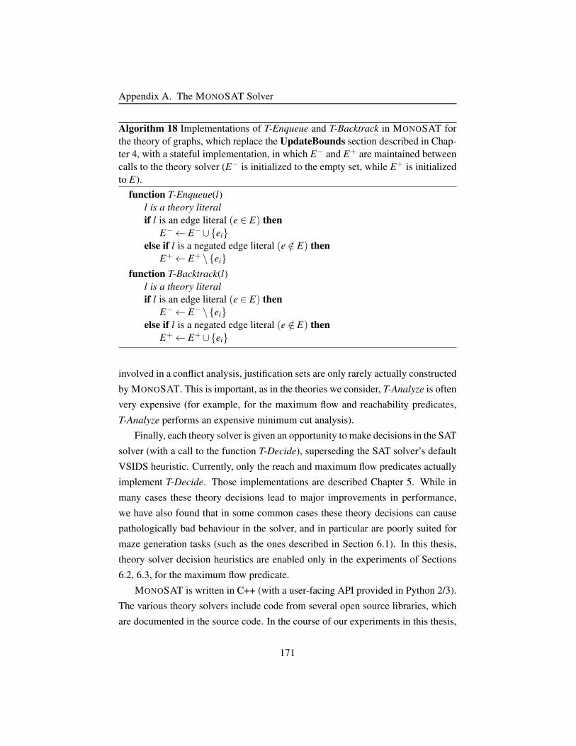
Appendix A. The MONOSAT Solver
Algorithm 18 Implementations of T-Enqueue and T-Backtrack in MONOSAT forthe theory of graphs, which replace the UpdateBounds section described in Chap-ter 4, with a stateful implementation, in which E− and E+ are maintained betweencalls to the theory solver (E− is initialized to the empty set, while E+ is initializedto E).
function T-Enqueue(l)l is a theory literalif l is an edge literal (e ∈ E) then
E−← E−∪eielse if l is a negated edge literal (e /∈ E) then
E+← E+ \eifunction T-Backtrack(l)
l is a theory literalif l is an edge literal (e ∈ E) then
E−← E− \eielse if l is a negated edge literal (e /∈ E) then
E+← E+∪ei
involved in a conflict analysis, justification sets are only rarely actually constructed
by MONOSAT. This is important, as in the theories we consider, T-Analyze is often
very expensive (for example, for the maximum flow and reachability predicates,
T-Analyze performs an expensive minimum cut analysis).
Finally, each theory solver is given an opportunity to make decisions in the SAT
solver (with a call to the function T-Decide), superseding the SAT solver’s default
VSIDS heuristic. Currently, only the reach and maximum flow predicates actually
implement T-Decide. Those implementations are described Chapter 5. While in
many cases these theory decisions lead to major improvements in performance,
we have also found that in some common cases these theory decisions can cause
pathologically bad behaviour in the solver, and in particular are poorly suited for
maze generation tasks (such as the ones described in Section 6.1). In this thesis,
theory solver decision heuristics are enabled only in the experiments of Sections
6.2, 6.3, for the maximum flow predicate.
MONOSAT is written in C++ (with a user-facing API provided in Python 2/3).
The various theory solvers include code from several open source libraries, which
are documented in the source code. In the course of our experiments in this thesis,
171
Appendix A. The MONOSAT Solver
various, improving versions of MONOSAT were tested. In Section 6.1, MONO-
SAT was compiled with G++ 4.8.1; in the remaining experiments, it was compiled
with g++ 6.0. Experiments were conducted using the Python API of MONOSAT,
with Python 3.3 (Section 6.1) and Python 3.4 (all other experiments).
MONOSAT is freely available under an open-source license, and can be found
at www.cs.ubc.ca/labs/isd/projects/monosat.
172
Appendix B
Monotonic Theory of Bitvectors
We describe a simple monotonic theory of bitvectors. This theory solver is de-
signed to be efficiently combinable with the theory of graphs (Chapter 5), by deriv-
ing tight bounds on each bitvector variable as assignments are made in the solver,
and passing those bounds to other theory solvers in the form of comparison atoms
on shared bitvector variables (as described in Section 4.5).
The theory of bitvectors we introduce here is a theory of fixed-width, non-
wrapping bitvectors, supporting only comparison predicates and addition. In con-
trast, the standard theory of bitvectors widely considered in the literature (e.g.,
[30, 42, 70, 100]), which is essentially a theory of finite modular arithmetic, sup-
ports many inherently non-monotonic operators (such as bitwise xor).
In the standard theory of bitvectors, the formula
x+2 = y
with x,y both 3-bit unsigned bitvectors, both x = 5,y = 7, and x = 7,y = 1 are
satisfying assignments, as 7+ 2 ≡ 1 (mod 8). In contrast, in our non-wrapping
theory of bitvectors, x = 5,y = 7 is satisfying, while x = 7,y = 1 is not.
Formally, the theory of non-wrapping bitvectors for bit-width n is a subset of
the theory of integer arithmetic, in which every variable and constant x is con-
strained to the range 0 ≤ x < 2n, for fixed n. As all variables are restricted to a
finite range of values, this fragment could be easily bit-blasted into propositional
173
Appendix B. Monotonic Theory of Bitvectors
logic, however we instead will handle it as a lazy SMT theory, using the SMMT
framework. While the performance of this theory solver on its own is in fact not
competitive with bit-blasting bitvector theory solvers, handling this theory lazily
has the advantage that it allows for comparison atoms to be created on the fly with-
out needing to bit-blast comparator circuits for each one. This is important, as this
bitvector theory will be combined with other monotonic theory solvers by deriving
and passing large numbers of comparison atoms for each bitvector. In practice, a
very large number of such comparison atoms will be created by the solver, and we
found it to be prohibitively expensive to construct bit-blasted comparator circuits
for each of these comparison atoms, thus motivating the creation of a new theory
solver.
In addition to comparison predicates, this theory of bitvectors supports one
function: addition. Formally, the function add(a,b) 7→ c takes two bitvector ar-
guments (a,b) of the same width and outputs a third bitvector (c) of the same
bit-width. In our non-wrapping bitvector theory, if a and b are the n-width bitvec-
tor arguments of an addition function, it is enforced that a+ b < 2n (by treating
a+b≥ 2n as a conflict in the theory).
In Section 4.3, we described two approaches to supporting function composi-
tion in monotonic theory solvers:
1. Flatten any function composition by introducing fresh variables, treating the
functions as predicates relating those variables, and then apply Algorithm 3.
2. Directly support propagation with function composition, using Algorithm 8.
While we take the latter approach in Chapter 8, we take the former approach
here (for historical reasons, as the bitvector theory solver was developed before we
began work on the CTL theory solver).
Our implementation of theory propagation for the (non-wrapping) theory of
bitvectors is described in below. For each n-bit bitvector b, we introduce atoms
(b0 ∈ b),(b1 ∈ b) . . .(bn−1 ∈ b) to expose the assignment of each bit to the SAT
solver. For notational convenience, we represent the negation of (bi ∈ b) as (bi /∈ b).
174

Appendix B. Monotonic Theory of Bitvectors
Algorithm 19 Theory propagation for the theory of non-wrapping bitvectors.
function T-Propagate(M)
M is a partial assignment; theory propagate returns a tuple (FALSE, con-
flictSet) ifM is found to be UNSAT, and otherwise returns (TRUE,M), possibly
deriving additional atoms to add toM. In practice, we maintain bounds b−,b+
from previous calls, only updating them if an atom involving b has been added
to or removed fromM.
assignmentChanged← FALSE
for each n-bit bitvector variable b dob−← 0,b+← 0
for i in 0..n−1 doif (bi /∈ b) /∈M then
b+← b++2i
if (bi ∈ b) ∈M thenb−← b−+2i
for each comparison to constant (b≤ σi) doif (b≤ σi) ∈M then
b+← min(b+,σi)
else if (b > σi) ∈M thenb−← max(b−,σi +1)
elseif b+ ≤ σi then
assignmentChanged← TRUE
M←M∪(b≤ σi)else if b− > σi then
assignmentChanged← TRUE
M←M∪(b > σi)
for each comparison atom between bitvectors (a≤ b) doif (a≤ b) ∈M then
a+← min(a+,b+)
b−← max(b−,a−)
else if (a > b) ∈M then
175
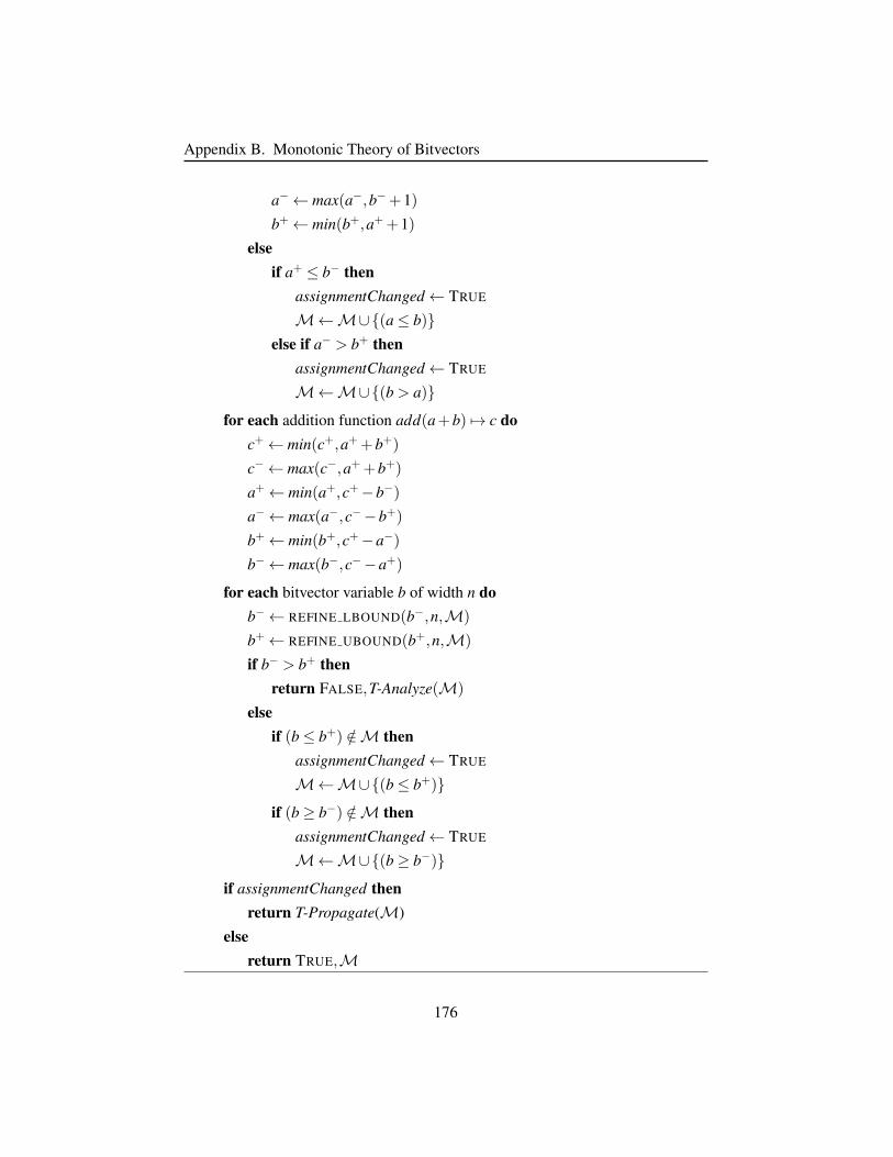
Appendix B. Monotonic Theory of Bitvectors
a−← max(a−,b−+1)
b+← min(b+,a++1)
elseif a+ ≤ b− then
assignmentChanged← TRUE
M←M∪(a≤ b)else if a− > b+ then
assignmentChanged← TRUE
M←M∪(b > a)
for each addition function add(a+b) 7→ c doc+← min(c+,a++b+)
c−← max(c−,a++b+)
a+← min(a+,c+−b−)
a−← max(a−,c−−b+)
b+← min(b+,c+−a−)
b−← max(b−,c−−a+)
for each bitvector variable b of width n dob−← REFINE LBOUND(b−,n,M)
b+← REFINE UBOUND(b+,n,M)
if b− > b+ thenreturn FALSE,T-Analyze(M)
elseif (b≤ b+) /∈M then
assignmentChanged← TRUE
M←M∪(b≤ b+)
if (b≥ b−) /∈M thenassignmentChanged← TRUE
M←M∪(b≥ b−)
if assignmentChanged thenreturn T-Propagate(M)
elsereturn TRUE,M
176
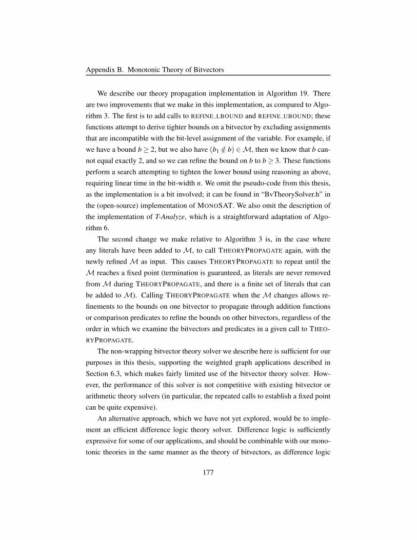
Appendix B. Monotonic Theory of Bitvectors
We describe our theory propagation implementation in Algorithm 19. There
are two improvements that we make in this implementation, as compared to Algo-
rithm 3. The first is to add calls to REFINE LBOUND and REFINE UBOUND; these
functions attempt to derive tighter bounds on a bitvector by excluding assignments
that are incompatible with the bit-level assignment of the variable. For example, if
we have a bound b≥ 2, but we also have (b1 /∈ b) ∈M, then we know that b can-
not equal exactly 2, and so we can refine the bound on b to b≥ 3. These functions
perform a search attempting to tighten the lower bound using reasoning as above,
requiring linear time in the bit-width n. We omit the pseudo-code from this thesis,
as the implementation is a bit involved; it can be found in “BvTheorySolver.h” in
the (open-source) implementation of MONOSAT. We also omit the description of
the implementation of T-Analyze, which is a straightforward adaptation of Algo-
rithm 6.
The second change we make relative to Algorithm 3 is, in the case where
any literals have been added to M, to call THEORYPROPAGATE again, with the
newly refined M as input. This causes THEORYPROPAGATE to repeat until the
M reaches a fixed point (termination is guaranteed, as literals are never removed
fromM during THEORYPROPAGATE, and there is a finite set of literals that can
be added to M). Calling THEORYPROPAGATE when the M changes allows re-
finements to the bounds on one bitvector to propagate through addition functions
or comparison predicates to refine the bounds on other bitvectors, regardless of the
order in which we examine the bitvectors and predicates in a given call to THEO-
RYPROPAGATE.
The non-wrapping bitvector theory solver we describe here is sufficient for our
purposes in this thesis, supporting the weighted graph applications described in
Section 6.3, which makes fairly limited use of the bitvector theory solver. How-
ever, the performance of this solver is not competitive with existing bitvector or
arithmetic theory solvers (in particular, the repeated calls to establish a fixed point
can be quite expensive).
An alternative approach, which we have not yet explored, would be to imple-
ment an efficient difference logic theory solver. Difference logic is sufficiently
expressive for some of our applications, and should be combinable with our mono-
tonic theories in the same manner as the theory of bitvectors, as difference logic
177
Appendix B. Monotonic Theory of Bitvectors
supports comparisons to constants. A fast difference logic solver would almost
certainly outperform the above bitvector theory (considered in isolation from other
monotonic theory solvers). However, while existing difference logic theory solvers
(e.g., as described in [10, 144, 190, 200]) are designed to quickly determine the
satisfiability of a set of difference logic constraints; they are not (to the best of
our knowledge) designed to efficiently derive not just satisfying, but tight, upper
and lower bounds on each variable, from partial assignments during theory prop-
agation. In contrast, the bitvector theory solver we described in this section is
designed to find and maintain tight upper and lower bounds on each variable, from
partial assignments. This is critically important, as passing tight bounds to other
monotonic theory solvers (such as the weighted graph theory of Chapter 5) can
allow those other theory solvers to prune unsatisfying assignments early.
178

Appendix C
Supporting Materials
C.1 Proof of Lemma 4.1.1This lemma can be proven for the case of totally ordered σ , by considering the
following exhaustive, mutually exclusive cases:
Proof. 1. T |= ¬MA. In this case, MA is by itself already an inconsistent
assignment to the comparison atoms. This can happen if some variable x is
assigned to be both larger and smaller than some constant, or is assigned to
be larger than σ> or smaller than σ⊥. In this case, as MA (and hence any
superset ofMA) is theory unsatisfiable,MA =⇒T
p holds trivially for any p,
and hence both the left and right hand sides of 4.1 and 4.2 hold.
2. MA T , T ∪MA |= ¬(x ≥ σ j). In this case, MA ∪x ≥ σi =⇒T
p holds
trivially for any p, and so 4.1 holds.
3. MA T , T ∪MA |= ¬(x ≥ σi). In this case, MA ∪ x ≥ σi =⇒T
p holds
trivially for any p. AsMA is by itself theory satisfiable, andMA only con-
tains assignments of variables to constants, there must exist some σk < σi,
such that atom (x ≤ σk) ∈ MA. As σ j ≥ σi, we also have σ j > σk, and
T ∪MA |=¬(x≥ σ j). Therefore,MA∪x≥ σi=⇒T
p holds trivially for any
p, and so 4.1 holds.
179
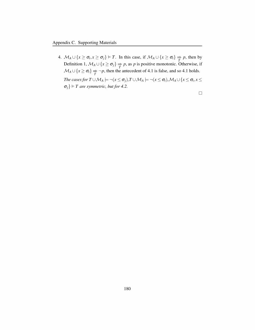
Appendix C. Supporting Materials
4. MA ∪x ≥ σi,x ≥ σ j T . In this case, if MA ∪x ≥ σi =⇒T
p, then by
Definition 1,MA∪x≥ σ j=⇒T
p, as p is positive monotonic. Otherwise, if
MA∪x≥ σi=⇒T¬p, then the antecedent of 4.1 is false, and so 4.1 holds.
The cases for T ∪MA |=¬(x≤ σ j),T ∪MA |=¬(x≤ σi),MA∪x≤ σi,x≤σ j T are symmetric, but for 4.2.
180
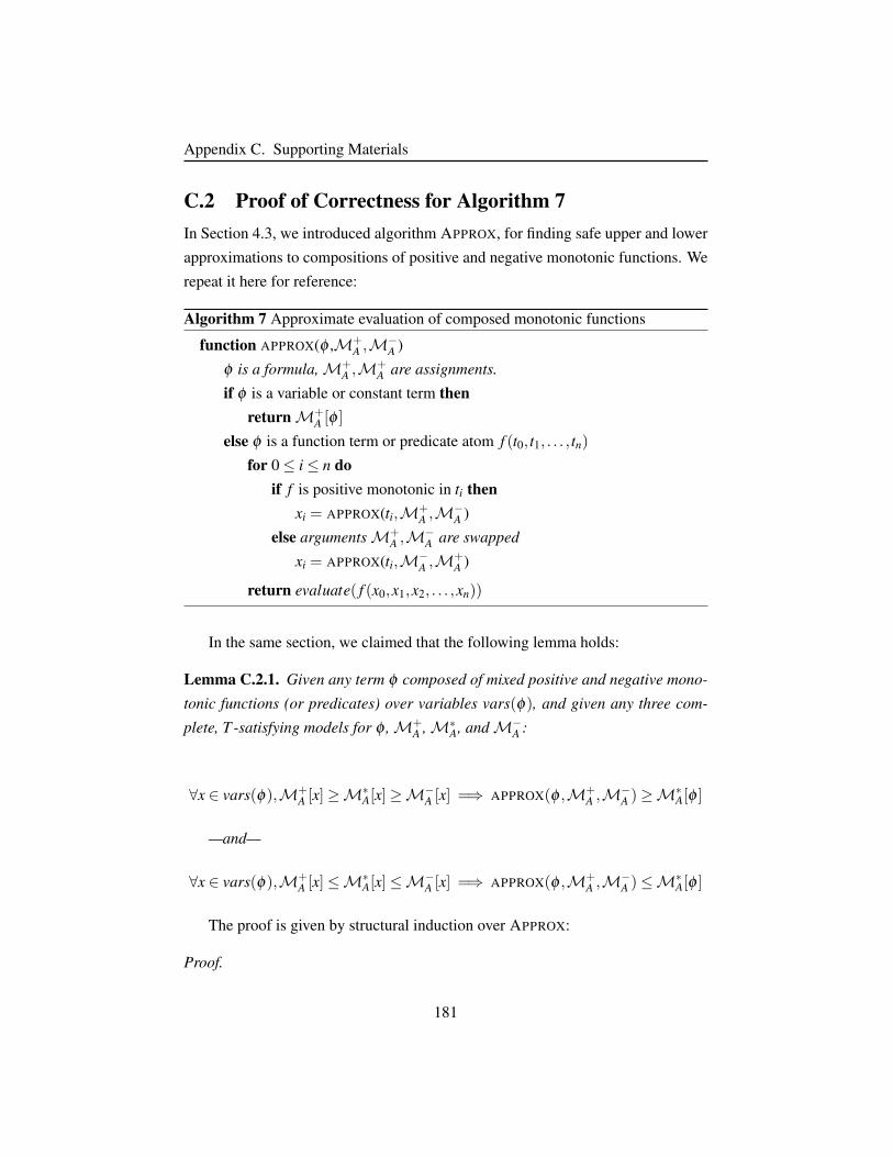
Appendix C. Supporting Materials
C.2 Proof of Correctness for Algorithm 7In Section 4.3, we introduced algorithm APPROX, for finding safe upper and lower
approximations to compositions of positive and negative monotonic functions. We
repeat it here for reference:
Algorithm 7 Approximate evaluation of composed monotonic functions
function APPROX(φ ,M+A ,M
−A )
φ is a formula,M+A ,M
+A are assignments.
if φ is a variable or constant term thenreturnM+
A [φ ]
else φ is a function term or predicate atom f (t0, t1, . . . , tn)
for 0≤ i≤ n doif f is positive monotonic in ti then
xi = APPROX(ti,M+A ,M
−A )
else argumentsM+A ,M
−A are swapped
xi = APPROX(ti,M−A ,M
+A )
return evaluate( f (x0,x1,x2, . . . ,xn))
In the same section, we claimed that the following lemma holds:
Lemma C.2.1. Given any term φ composed of mixed positive and negative mono-
tonic functions (or predicates) over variables vars(φ), and given any three com-
plete, T -satisfying models for φ ,M+A ,M∗
A, andM−A :
∀x ∈ vars(φ),M+A [x]≥M
∗A[x]≥M−
A [x] =⇒ APPROX(φ ,M+A ,M
−A )≥M
∗A[φ ]
—and—
∀x ∈ vars(φ),M+A [x]≤M
∗A[x]≤M−
A [x] =⇒ APPROX(φ ,M+A ,M
−A )≤M
∗A[φ ]
The proof is given by structural induction over APPROX:
Proof.
181
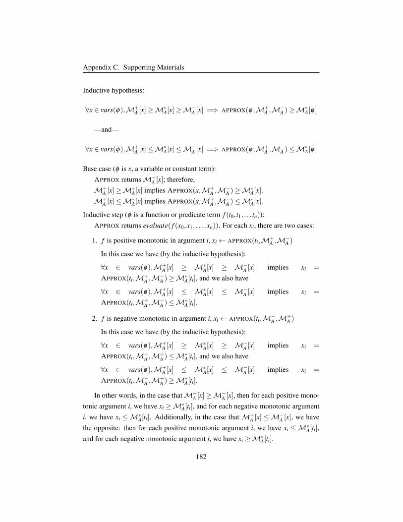
Appendix C. Supporting Materials
Inductive hypothesis:
∀x ∈ vars(φ),M+A [x]≥M
∗A[x]≥M−
A [x] =⇒ APPROX(φ ,M+A ,M
−A )≥M
∗A[φ ]
—and—
∀x ∈ vars(φ),M+A [x]≤M
∗A[x]≤M−
A [x] =⇒ APPROX(φ ,M+A ,M
−A )≤M
∗A[φ ]
Base case (φ is x, a variable or constant term):
APPROX returnsM+A [x]; therefore,
M+A [x]≥M∗
A[x] implies APPROX(x,M+A ,M
−A )≥M∗
A[x].
M+A [x]≤M∗
A[x] implies APPROX(x,M+A ,M
−A )≤M∗
A[x].
Inductive step (φ is a function or predicate term f (t0, t1, . . . tn)):
APPROX returns evaluate( f (x0,x1, . . . ,xn)). For each xi, there are two cases:
1. f is positive monotonic in argument i, xi← APPROX(ti,M+A ,M
−A )
In this case we have (by the inductive hypothesis):
∀x ∈ vars(φ),M+A [x] ≥ M∗
A[x] ≥ M−A [x] implies xi =
APPROX(ti,M+A ,M
−A )≥M∗
A[ti], and we also have
∀x ∈ vars(φ),M+A [x] ≤ M∗
A[x] ≤ M−A [x] implies xi =
APPROX(ti,M+A ,M
−A )≤M∗
A[ti].
2. f is negative monotonic in argument i, xi← APPROX(ti,M−A ,M
+A )
In this case we have (by the inductive hypothesis):
∀x ∈ vars(φ),M+A [x] ≥ M∗
A[x] ≥ M−A [x] implies xi =
APPROX(ti,M−A ,M
+A )≤M∗
A[ti], and we also have
∀x ∈ vars(φ),M+A [x] ≤ M∗
A[x] ≤ M−A [x] implies xi =
APPROX(ti,M−A ,M
+A )≥M∗
A[ti].
In other words, in the case thatM+A [x]≥M
−A [x], then for each positive mono-
tonic argument i, we have xi ≥M∗A[ti], and for each negative monotonic argument
i, we have xi ≤M∗A[ti]. Additionally, in the case that M+
A [x] ≤M−A [x], we have
the opposite: then for each positive monotonic argument i, we have xi ≤M∗A[ti],
and for each negative monotonic argument i, we have xi ≥M∗A[ti].
182
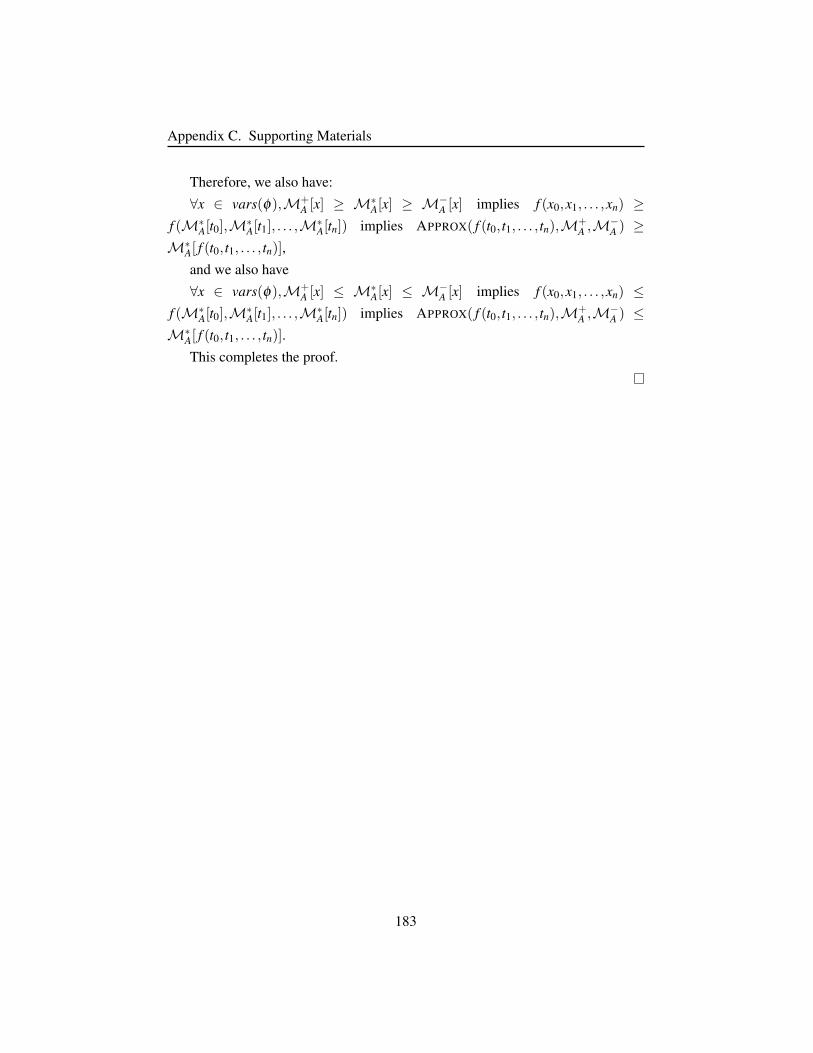
Appendix C. Supporting Materials
Therefore, we also have:
∀x ∈ vars(φ),M+A [x] ≥ M∗
A[x] ≥ M−A [x] implies f (x0,x1, . . . ,xn) ≥
f (M∗A[t0],M∗
A[t1], . . . ,M∗A[tn]) implies APPROX( f (t0, t1, . . . , tn),M+
A ,M−A ) ≥
M∗A[ f (t0, t1, . . . , tn)],
and we also have
∀x ∈ vars(φ),M+A [x] ≤ M∗
A[x] ≤ M−A [x] implies f (x0,x1, . . . ,xn) ≤
f (M∗A[t0],M∗
A[t1], . . . ,M∗A[tn]) implies APPROX( f (t0, t1, . . . , tn),M+
A ,M−A ) ≤
M∗A[ f (t0, t1, . . . , tn)].
This completes the proof.
183
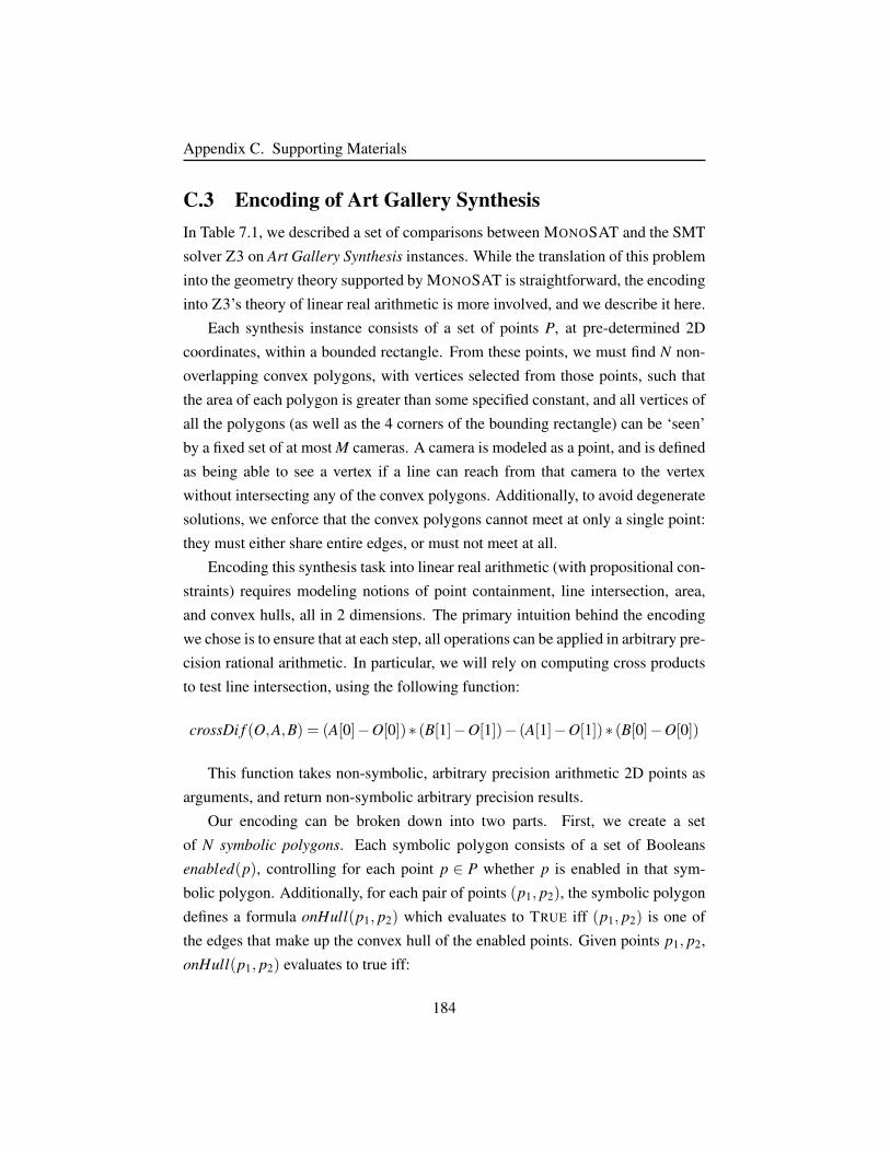
Appendix C. Supporting Materials
C.3 Encoding of Art Gallery SynthesisIn Table 7.1, we described a set of comparisons between MONOSAT and the SMT
solver Z3 on Art Gallery Synthesis instances. While the translation of this problem
into the geometry theory supported by MONOSAT is straightforward, the encoding
into Z3’s theory of linear real arithmetic is more involved, and we describe it here.
Each synthesis instance consists of a set of points P, at pre-determined 2D
coordinates, within a bounded rectangle. From these points, we must find N non-
overlapping convex polygons, with vertices selected from those points, such that
the area of each polygon is greater than some specified constant, and all vertices of
all the polygons (as well as the 4 corners of the bounding rectangle) can be ‘seen’
by a fixed set of at most M cameras. A camera is modeled as a point, and is defined
as being able to see a vertex if a line can reach from that camera to the vertex
without intersecting any of the convex polygons. Additionally, to avoid degenerate
solutions, we enforce that the convex polygons cannot meet at only a single point:
they must either share entire edges, or must not meet at all.
Encoding this synthesis task into linear real arithmetic (with propositional con-
straints) requires modeling notions of point containment, line intersection, area,
and convex hulls, all in 2 dimensions. The primary intuition behind the encoding
we chose is to ensure that at each step, all operations can be applied in arbitrary pre-
cision rational arithmetic. In particular, we will rely on computing cross products
to test line intersection, using the following function:
crossDi f (O,A,B) = (A[0]−O[0])∗ (B[1]−O[1])− (A[1]−O[1])∗ (B[0]−O[0])
This function takes non-symbolic, arbitrary precision arithmetic 2D points as
arguments, and return non-symbolic arbitrary precision results.
Our encoding can be broken down into two parts. First, we create a set
of N symbolic polygons. Each symbolic polygon consists of a set of Booleans
enabled(p), controlling for each point p ∈ P whether p is enabled in that sym-
bolic polygon. Additionally, for each pair of points (p1, p2), the symbolic polygon
defines a formula onHull(p1, p2) which evaluates to TRUE iff (p1, p2) is one of
the edges that make up the convex hull of the enabled points. Given points p1, p2,
onHull(p1, p2) evaluates to true iff:
184
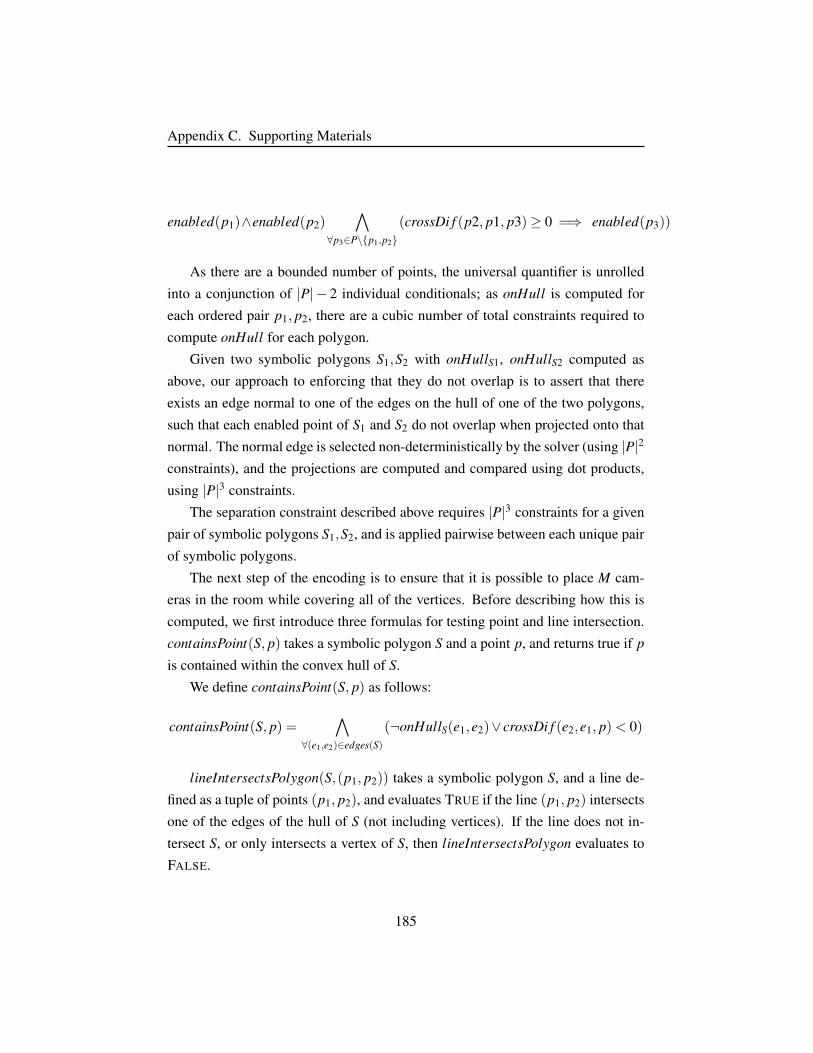
Appendix C. Supporting Materials
enabled(p1)∧enabled(p2)∧
∀p3∈P\p1,p2(crossDi f (p2, p1, p3)≥ 0 =⇒ enabled(p3))
As there are a bounded number of points, the universal quantifier is unrolled
into a conjunction of |P| − 2 individual conditionals; as onHull is computed for
each ordered pair p1, p2, there are a cubic number of total constraints required to
compute onHull for each polygon.
Given two symbolic polygons S1,S2 with onHullS1, onHullS2 computed as
above, our approach to enforcing that they do not overlap is to assert that there
exists an edge normal to one of the edges on the hull of one of the two polygons,
such that each enabled point of S1 and S2 do not overlap when projected onto that
normal. The normal edge is selected non-deterministically by the solver (using |P|2
constraints), and the projections are computed and compared using dot products,
using |P|3 constraints.
The separation constraint described above requires |P|3 constraints for a given
pair of symbolic polygons S1,S2, and is applied pairwise between each unique pair
of symbolic polygons.
The next step of the encoding is to ensure that it is possible to place M cam-
eras in the room while covering all of the vertices. Before describing how this is
computed, we first introduce three formulas for testing point and line intersection.
containsPoint(S, p) takes a symbolic polygon S and a point p, and returns true if p
is contained within the convex hull of S.
We define containsPoint(S, p) as follows:
containsPoint(S, p) =∧
∀(e1,e2)∈edges(S)
(¬onHullS(e1,e2)∨ crossDi f (e2,e1, p)< 0)
lineIntersectsPolygon(S,(p1, p2)) takes a symbolic polygon S, and a line de-
fined as a tuple of points (p1, p2), and evaluates TRUE if the line (p1, p2) intersects
one of the edges of the hull of S (not including vertices). If the line does not in-
tersect S, or only intersects a vertex of S, then lineIntersectsPolygon evaluates to
FALSE.
185
Appendix C. Supporting Materials
We define lineIntersectsPolygon(S,(p1, p2)) as follows:
lineIntersectsPolygon(S,(p1, p2)) = containsPoint(S, p1)∨ containsPoint(S, p2)∨∀(e1,e2)∈edges(S)
(onHullS(e1,e2)∧ lineIntersectsLine((p1, p2),(e1,e2)))
Finally, lineIntersectsLine((p1, p2),(e1,e2)) returns true if the two (non sym-
bolic) lines defined by endpoints p1, p2 and e1,e2 intersect each other. This can be
tested for non-symbolic rational constants using cross products.
Given a fixed camera position pc, and a fixed vertex to observe pv,
isVisible(pc, pv) is evaluated as follows:
isVisible(pc, pv) =∧
∀S∈Polygons
¬lineIntersectsPolygon(S,(pc, pv))
We then use a cardinality constraint to force the solver to pick C positions from
the point set P to be cameras, and use the line intersection formula described above
to force that every vertex that is on hull of a symbolic polygon must be visible from
at least one vertex that is a camera (meaning that no symbolic polygon intersects
the line between the camera and that vertex).
Each instance also specifies a minimum area A for each symbolic polygon (to
ensure we do not get degenerate solutions consisting of very thin polygon seg-
ments). We compute the area of the convex hull of each symbolic polygon S as:
area(S) =12 ∑∀(e1,e2)∈edges(S)
I f (onHullS(e1,e2),e1[0]∗ e2[1]− e1[1]∗ e2[0])
To complete the encoding, we assert:
∀S,area(S)≥ A
186
Appendix D
Monotonic Predicates
This is a listing of the monotonic predicates considered in this thesis, arranged by
topic.
D.1 Graph Predicates
D.1.1 Reachability
Monotonic Predicate: reachs,t(E) , true iff t can be reached from u in the graph
formed of the edges enabled in E.
Implementation of evaluate(reachs,t(E),G): We use the dynamic graph reacha-
bility/shortest paths algorithm of Ramalingam and Reps [171] to test whether
t can be reached from s in G. Ramalingam-Reps is a dynamic variant of Dijk-
stra’s Algorithm [79]); our implementation follows the one described in [48].
If there are multiple predicate atoms reachs,t(E) sharing the same source s,
then Ramalingam-Reps only needs to be updated once for the whole set of
atoms.
Implementation of analyze(reachs,tE,G−) Node s reaches t in G−, but
reachs,t(E) is assigned FALSE in M. Let e0,e1, . . . be a u− v path in G−;
return the conflict set (e0 ∈ E),(e1 ∈ E), . . . ,¬reachs,t(E).
Implementation of analyze(¬reachs,t(E),G+) Node t cannot be reached from s
187
Appendix D. Monotonic Predicates
in G+, but reachs,t(E) is assigned TRUE. Let e0,e1, . . . be a cut of disabled
edges (ei /∈ E) separating u from v in G+. Return the conflict set (e0 /∈E),(e1 /∈ E), . . . ,reachs,t(E).
We find a minimum separating cut by creating a graph containing all edges
of E (including both the edges of G+ and the edges that are disabled in G+
in the current assignment), in which the capacity of each disabled edge of
E is 1, and the capacity of all other edges is infinity (forcing the minimum
cut to include only edges that correspond to disabled edge atoms). Any
standard maximum s-t flow algorithm can then be used to find a minimum
cut separating u from v. In our implementation, we use the dynamic Kohli-
Torr [140] minimum cut algorithm for this purpose.
Decision Heuristic: (Optional) If reachs,t(E) is assigned TRUE in M, but there
does not yet exist a u− v path in G−, then find a u− v path in G+ and pick
the first unassigned edge in that path to be assigned true as the next decision.
In practice, such a path has typically already been discovered, during the
evaluation of reachs,t on G+ during theory propagation.
D.1.2 Acyclicity
Monotonic Predicate: acyclic(E), true iff there are no (directed) cycles in the
graph formed by the enabled edges in E.
Implementation of evaluate(acyclic(E),G): Apply the PK dynamic topological
sort algorithm (as described in [164]). The PK algorithm is a fully dynamic
graph algorithm that maintains a topological sort of a directed graph as edges
are added to or removed from the graph; as a side effect, it also detects
directed cycles (in which case no topological sort exists). Return FALSE if
the PK algorithm successfully produces a topological sort, and return TRUE
if it fails (indicating the presence of a directed cycle).
Implementation of analyze(acyclic(E),G−) There is a cycle in E, but acyclic(E)
is assigned TRUE. Let e0,e1, . . . be the edges that make up a directed cycle
in E; return the conflict set (e0 ∈ E),(e1 ∈ E), . . . ,acyclic(E).
188
Appendix D. Monotonic Predicates
Implementation of analyze(¬acyclic(E),G+) There is no cycle in E, but
acyclic(E) is assigned FALSE. Let e0,e1, . . . be the set of all edges not in
E+; return the conflict set (e0 /∈ E),(e1 /∈ E), . . . ,¬acyclic(E). (Note that
this is the default monotonic conflict set.)
D.1.3 Connected Components
Here we consider a predicate which constraints the number of (simple) connected
components in the graph to be less than or greater than some constant. There are
both directed and undirected variations of this predicate; we describe the directed
version, which counts the number of strongly connected components.
Monotonic Predicate: connectedComponentsE,m, true iff the number of con-
nected components in the graph formed of edges E is≤m, with m a bitvector.
Implementation of evaluate(connectedComponents(E,m),G): Use Tarjan’s
SCC algorithm [195] to count the number of distint strongly connected
components in G; return TRUE iff the count is ≤ m.
Implementation of analyze(connectedComponents(E,m),G−): The connected
component count is less or equal to m, but connectedComponents(E,m)
is FALSE in M. Construct a spanning tree for each component of
G− (using depth-first search). Let edges e1,e2, . . . be the edges in
these spanning trees; return the conflict set (e1 ∈ E),(e2 ∈ E), . . . ,(m >
m−),¬connectedComponents(E,m).
Implementation of analyze(¬connectedComponents(E,m),G+): The con-
nected component count is greater than m, but connectedComponents(E,m)
is TRUE in M Collect all disabled edges ei = (u,v) where u
and v belong to different components in G+; the conflict set is
(e1 /∈ E),(e2 /∈ E), . . . ,(m < m+),connectedComponents(E,m).
Above we describe the implementation for directed graphs; for undirected
graphs, Tarjan’s SCC algorithm does not apply. For undirected graphs, we count
the number of connected components using disjoint-sets/union-find.
189

Appendix D. Monotonic Predicates
D.1.4 Shortest Path
Monotonic Predicate: shortestPaths,t(E, l,c0,c1, . . .), true iff the length of the
shortest s− t path in the graph formed of the edges enabled in E with edge
weights c0,c1, . . . is less than or equal to bit-vector l.
Implementation of evaluate(shortestPaths,t(E, l,c0,c1, . . .),G): We use the dy-
namic graph reachability/shortest paths algorithm of Ramalingam and
Reps [171] to test whether the shortest path to t from s is less than l. If there
are multiple predicate atoms shortestPaths,t(E) sharing the same source s,
then Ramalingam-Reps only needs to be updated once for the whole set of
atoms.
Implementation of analyze(shortestPaths,t ,E, l,c0,c1, . . .): There exists an s-t
path in G− of length ≤ l, but shortestPaths,t is assigned FALSE in
M. Let e0,e1, . . . be a shortest s − t path in G− with weights
w0,w1, . . .; return the conflict set (e0 ∈ E),(w0 ≥ w−0 ),(e1 ∈ E),(w1 ≥w−1 ), . . . ,¬shortestPaths,t.
Implementation of analyze(¬shortestPaths,t ,E, l,c0,c1, . . .): Walk back from u
in G+ along enabled and unassigned edges with edge weights w0,w1, . . .;
collect all incident disabled edges e0,e1, . . .; return the conflict set (e0 /∈E),(e1 /∈ E), . . . ,(w0 ≤ w+
0 ),(w1 ≤ w+1 ) . . . ,shortestPathu,v,G≤C(edges).
D.1.5 Maximum Flow
Monotonic Predicate: maxFlows,t(E,m,c0,c1, . . .), true iff the maximum s-t flow
in G with edge capacities c0,c1, . . . is ≥ m.
Implementation of evaluate(maxFlows,t ,G,m,c0,c1, . . .): We apply the dynamic
minimum-cut/maximum s-t algorithm by Kohli and Torr [140] to compute
the maximum flow of G, with edge capacities set by ci. Return TRUE iff that
flow is greater or equal to m.
Implementation of analyze(maxFlows,t ,G−,m+,c−0 ,c−1 , . . .): The maximum s-t
flow in G− is f , with f ≥ m+). In the computed flow, each edge ei is either
190

Appendix D. Monotonic Predicates
disabled in G−, or it has been allocated a (possibly zero-valued) flow fi, with
fi ≤ c−i . Let ea,eb, . . . be the edges enabled in G− with non-zero allocated
flows fa, fb, . . .. Either one of those edges must be disabled in the graph, or
one of the capacities of those edges must be decreased, or the flow will be
at least f . Return the conflict set (ea ∈ E),(eb ∈ E), . . . ,(ca ≥ fa),(cb ≥fb) . . . ,(m≤ f ),maxFlows,t(E,m,c0,c1, . . .).
Implementation of analyze(¬maxFlows,t ,G+,m−,c+0 ,c+1 , . . .): The maximum s-
t flow in G+ is f , with f < m−. In the flow, each edge that is enabled in G+
has been allocated a (possibly zero-valued) flow fi, with fi ≤ c+i .
Create a graph Gcut . For each edge ei = (u,v) in G+, with fi < c+i , add a
forward edge (u,v) to Gcut with infinite capacity, and also a backward edge
(v,u) with capacity fi. For each edge ei = (u,v) in G+ with fi = c+i , add a
forward edge (u,v) to Gcut with capacity 1, and also a backward edge (v,u)
with capacity fi. For each edge ei = (u,v) that is disabled in G+, add only
the forward edge (u,v) to Gcut , with capacity 1.
Compute the minimum s-t cut of Gcut . Some of the edges along this cut may
have been edges disabled in G+, while some may have been edges enabled
in G+ with fully utilized edge capacity. Let ea,eb, . . . be the edges of the
minimum cut of Gcut that were disabled in G+. Let cc,cd , . . . be the capacities
of edges in the minimum cut for which the edge was included in G+, with
fully utilized capacity. Return the conflict set (ea /∈ E),(eb /∈ E), . . . ,(cc ≤fc),(cd ≤ fd), . . . ,(m > f ),¬maxFlows,t(E,m,c0,c1, . . .).
In practice, we maintain a graph Gcut for each maximum flow predicate atom,
updating its edges only lazily when needed for conflict analysis.
Decision Heuristic: (Optional) If maxFlows,t is assigned TRUE inM, but there
does not yet exist a sufficient flow in G−, then find a maximum flow in G+,
and pick the first unassigned edge with non-zero flow to be assigned TRUE
as the next decision. If no such edge exists, then pick the first unassigned
edge capacity and assign its capacity to its flow G+, as the next decision. In
practice, such a flow is typically already discovered, during the evaluation of
maxFlows,t on G+ during theory propagation.
191
Appendix D. Monotonic Predicates
D.1.6 Minimum Spanning Tree Weight
Here we consider constraints on the weight of the minimum spanning tree in a
weighted (non-negative) undirected graph. For the purposes of this solver, we will
define unconnected graphs to have infinite weight.
Monotonic Predicate: minSpanningTree(E,m,c0,c1, . . .), evaluates to TRUE iff
the minimum weight spanning tree in the graph formed of edges E with
edge weights given by c0,c1, . . ., has weight ≤ m.
Implementation of evaluate(minSpanningTree(E,m,c0,c1, . . .),G: We use Spira
and Pan’s [187] fully dynamic algorithm for minimum spanning trees to de-
temrine the minimum weight spanning tree of G; return TRUE iff that weight
is ≤ m.
Implementation of analyze(minSpanningTree,G−,m−,c+0 ,c+1 , . . .): The
minimum weight spanning tree of G− is less or equal to m−, but
minSpanningTree is FALSE in M. Let e0,e1, . . ., with edge weights
w0,w1, . . ., be the edges of that spanning tree. Return the conflict set
(e0 ∈ E),(w0≤w+0 ),(e1 ∈ E),(w1≤w+
1 ),(m≥m−),¬minSpanningTree.
Implementation of analyze(¬minSpanningTree,G+,m−,c−0 ,c−1 , . . .): The mini-
mum weight spanning tree of G+ is > m+, but minSpanningTree is TRUE in
M. There are two cases to consider:
1. If G+ is disconnected, then we consider its weight to be infinite. In
this case, we find a cut e1,e2, . . . of disabled edges separating any
one component from the remaining components. Given a component
in G+, a valid separating cut consists of all disabled edges (u,v) such
that u is in the component and v is not. We can either return the
first such cut we find, or the smallest one from among all the com-
ponents. For disconnected G+, return the conflict set (e1 /∈ E),(e2 /∈E), . . . ,minSpanningTree(E,m).
2. If G+ is not disconnected, then we search for a minimal set of edges
required to decrease the weight of the minimum spanning tree. To
do so, we visit each disabled edge (u,v), and then examine the cycle
192
Appendix D. Monotonic Predicates
that would be created if we were to add (u,v) into the minimum span-
ning tree. (Because the minimum spanning tree reaches all nodes, and
reaches them exactly once, adding a new edge between any two nodes
will create a unique cycle in the tree.) If any edge in that cycle has
higher weight than the disabled edge, then if that disabled edge were
to be enabled in the graph, we would be able to create a smaller span-
ning tree by replacing that larger edge in the cycle with the disabled
edge. Let e0,e1, . . . be the set of such disabled edges that can be used
to create lower weight spanning trees. Additionally, let w0,w1, . . . be
the weights of the edges in the minimum spanning tree of G+. Return
the conflict set is (e0 /∈ E),(e1 /∈ E), . . . ,(w0 ≥ w−0 ),(w1 ≥ w−1 ),(m≤m+),minSpanningTree(E,m).In practice, we can visit each such cycle in linear time by using Tar-
jan’s off-line lowest common ancestors algorithm [99] in the minimum
spanning tree found in G+. Visiting each edge in the cycle to check if
it is larger than each disabled edge takes linear time in the number of
edges in the tree for each cycle. Since the number of edges in the tree is
1 less than the number of nodes, the total runtime is then O(|V |2 · |D|),where D is the set of disabled edges in M.
D.2 Geometric Predicates
D.2.1 Area of Convex Hulls
Monotonic Predicate: hullArea≥x(S), hullArea>x(S), with S a finite set S ⊆ S′,
true iff the convex hull of the points in S has an area ≥ (resp. >) than x
(where x is a constant). This predicate is positive monotonic with respect to
the set S.
Algorithm: Initially, compute area(bound−),area(bound+). If area(bound−) >
x, compute area(H−); if area(bound+) < x, compute area(H+). The areas
can be computed explicitly, using arbitrary precision rational arithmetic.
Conflict set for hullArea≥x(S): The area of H− is greater or equal to x. Let
193
Appendix D. Monotonic Predicates
p0, p1, . . . be the points of S− that form the vertices of the under-approximate
hull H−, with area(H−) ≥ x. Then at least one of the points must be
disabled for the area of the hull to decrease below x. The conflict set is
(p0 ∈ S),(p1 ∈ S), . . . ,¬hullArea≥x(S).
Conflict set for ¬hullArea≥x(S): The area of H+ is less than x; then at least one
point pi /∈ S+ that is not contained in H+ must be added to the point set to
increase the area of H+. Let points p0, p1, . . . be the points of S′ not contained
in H+. The conflict set is (p0 /∈ S+),(p1 /∈ S+), . . . ,hullArea≥x(S), where
p0, p1, . . . are the (possibly empty) set of points pi /∈ S+.
D.2.2 Point Containment for Convex Hulls
Monotonic Predicate: hullContainsq(S), true iff the convex hull of the 2D points
in S contains the (fixed point) q.
Algorithm: First, check whether q is contained in the under-approximative bound-
ing box bound−. If it is, then check if q is contained in H−. We use the
PNPOLY [95] point inclusion test to perform this check, using arbitrary
precision rational arithmetic, which takes time linear in the number of ver-
tices of H−. In the same way, only if q is contained in bound+, check if q is
contained in H+ using PNPOLY.
Conflict set for hullContainsq(S): Convex hull H− contains p. Let p0, p1, p2 be
three points from H− that form a triangle containing p (such a triangle must
exist, as H− contains p, and we can triangulate H−, so one of those trian-
gles must contain p; this follows from Carathodory’s theorem for convex
hulls [51]). So long as those three points are enabled in S, H− must contain
them, and as they contain p, p must be contained in hunder. The conflict set
is (p0 ∈ S),(p1 ∈ S),(p2 ∈ S),¬hullContainsq(S).
Conflict set for ¬hullContainsq(S): p is outside of H+. If H+ is empty, then the
conflict set is the default monotonic conflict set. Otherwise, by the sepa-
rating axis theorem, there exists a separating axis between H+ and p. Let
p0, p1, . . . be the (disabled) points of S whose projection onto that axis is
194

Appendix D. Monotonic Predicates
≥ the projection of p onto that axis1. At least one of those points must
be enabled in S in order for H+ to grow to contain p. The conflict set is
(p0 /∈ S),(p1 /∈ S), . . . ,hullContainsq(S).
D.2.3 Line-Segment Intersection for Convex Hulls
Monotonic Predicate: hullIntersectsr(S), true iff the convex hull of the 2D points
in S intersects the (fixed) line-segment r.
Algorithm: First, check whether line-segment r intersects bound−. If it does,
check if r intersects H−. If H− is empty, is a point, or is itself a line-segment,
this is trivial (and can be checked precisely in arbitrary precision arithmetic
by computing cross products following [110]). Otherwise, we check if ei-
ther end-point of r is contained in H−, using PNPOLY as above for point
containment. If neither end-point is contained, we check whether the line-
segment intersects H−, by testing each edge of H− for intersection with r
(as before, by computing cross-products). If r does not intersect the under-
approximation, repeat the above on bound+ and H+.
Conflict set for hullIntersectsr(S): Convex hull H− intersects line-segment r. If
either end-point or r was contained in H−, then proceed as for the point con-
tainment predicate. Otherwise, the line-segment r intersects with at least one
edge (pi, p j) of H−. Conflict set is (pi ∈ S),(p j ∈ S),¬hullIntersectsr(S).
Conflict set for ¬hullIntersectsr(S): r is outside of H+. If H+ is empty, then the
conflict set is the naıve monotonic conflict set. Otherwise, by the separating
axis theorem, there exists a separating axis between H+ and line-segment r.
Let p0, p1, . . . be the (disabled) points of S whose projection onto that axis is
≥ the projection of the nearest endpoint of r onto that axis. At least one of
those points must be enabled in S in order for H+ to grow to contain p. The
conflict set is (p0 /∈ S),(p1 /∈ S), . . . ,hullIntersectsr(S).1We will make use of the separating axis theorem several times in this section. The standard pre-
sentation of the separating axis theorem involves normalizing the separating axis (which we wouldnot be able to do using rational arithmetic). This normalization is required if one wishes to computethe minimum distance between the projected point sets; however, if we are only interested in com-paring distances (and testing collisions), we can skip the normalization step, allowing the separatingaxis to be found and applied using only precise rational arithmetic.
195
Appendix D. Monotonic Predicates
D.2.4 Intersection of Convex Hulls
Monotonic Predicate: hullsIntersect(S0,S1), true iff the convex hull of the points
in S0 intersects the convex hull of the points of S1.
Algorithm: If the bounding box for convex hull H0 intersects the bounding box
for H1, then there are two possible cases to check for:
1. 1: A vertex of one hull is contained in the other, or
2. 2: an edge of H0 intersects an edge of H1.
If neither of the above cases holds, then H0 and H1 do not intersect.
Each of the above cases can be tested in quadratic time (in the number of
vertices of H0 and H1), using arbitrary precision arithmetic. In our imple-
mentation, we use PNPOLY, as described above, to test vertex containment,
and test for pair-wise edge intersection using cross products.
Conflict set for hullsIntersect(S0,S1): H−0 intersects H−1 . There are two (not mu-
tually exclusive) cases to consider:
1. A vertex of one hull is contained within the other hull. Let the point be
pa; let the hull containing it be H−b . Then (as argued above) there must
exist three vertices pb1, pb2, pb3 of H−b that form a triangle containing
pa. So long as those three points and pa are enabled, the two hulls
will overlap. Conflict set is (pa ∈ Sa),(pb1 ∈ Sb),(pb2 ∈ Sb),(pb3 ∈Sb),¬hullsIntersect(S0,S1).
2. An edge of H−0 intersects an edge of H−1 . Let p1a, p1b be points of H−0 ,
and p2a, p2b points of H−1 , such that line segments p1a, p1b and p2a, p2b
intersect. So long as these points are enabled, the hulls of the two
point sets must overlap. Conflict set is (p0a ∈ S0),(p0b ∈ S0),(p1a ∈S1),(p1b ∈ S1),¬hullsIntersect(S0,S1).
Conflict set for ¬hullsIntersect(S0,S1): H+0 do not intersect H+
1 . In this case,
there must exist a separating axis between H+0 and H+
1 . (Such an axis can be
discovered as a side effect of computing the cross products of each edge in
step 2 above.) Project all disabled points of S0 and S1 onto that axis. Assume
196
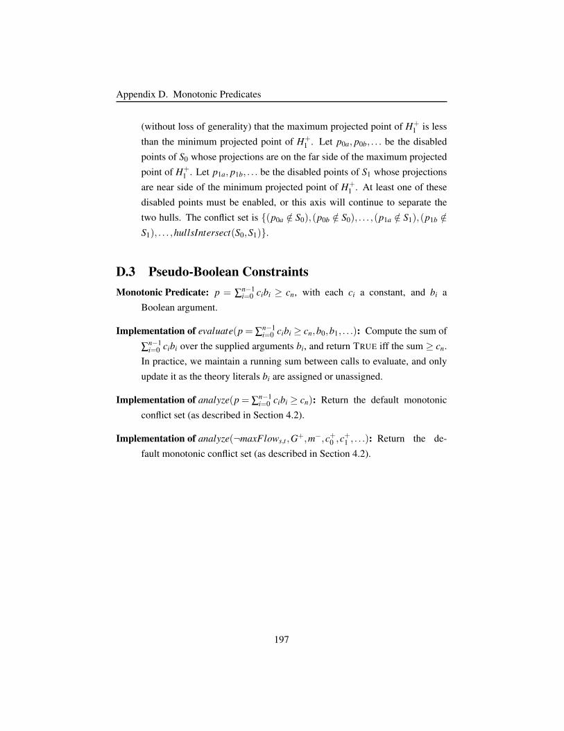
Appendix D. Monotonic Predicates
(without loss of generality) that the maximum projected point of H+1 is less
than the minimum projected point of H+1 . Let p0a, p0b, . . . be the disabled
points of S0 whose projections are on the far side of the maximum projected
point of H+1 . Let p1a, p1b, . . . be the disabled points of S1 whose projections
are near side of the minimum projected point of H+1 . At least one of these
disabled points must be enabled, or this axis will continue to separate the
two hulls. The conflict set is (p0a /∈ S0),(p0b /∈ S0), . . . ,(p1a /∈ S1),(p1b /∈S1), . . . ,hullsIntersect(S0,S1).
D.3 Pseudo-Boolean ConstraintsMonotonic Predicate: p = ∑
n−1i=0 cibi ≥ cn, with each ci a constant, and bi a
Boolean argument.
Implementation of evaluate(p = ∑n−1i=0 cibi ≥ cn,b0,b1, . . .): Compute the sum of
∑n−1i=0 cibi over the supplied arguments bi, and return TRUE iff the sum ≥ cn.
In practice, we maintain a running sum between calls to evaluate, and only
update it as the theory literals bi are assigned or unassigned.
Implementation of analyze(p = ∑n−1i=0 cibi ≥ cn): Return the default monotonic
conflict set (as described in Section 4.2).
Implementation of analyze(¬maxFlows,t ,G+,m−,c+0 ,c+1 , . . .): Return the de-
fault monotonic conflict set (as described in Section 4.2).
197

Appendix D. Monotonic Predicates
D.4 CTL Model CheckingIn Chapter 8, we describe a predciate for CTL model checking, along with
associated functions. We describe theory propagation in that chapter, however the
conflict analysis procedure for the theory of CTL model checking handles each
CTL operator separately, and as a result was too long to include in the main body
of Chapter 8. The complete procedure follows:
function ANALYZECTL(φ ,s,K+,K−,M)
Let (T+,P+) = K+
Let (T−,P−) = K−
c←if φ is EX(ψ) then
for each transition t outgoing from s doif (t /∈ T ) ∈M then
c← c∪(t ∈ T ).
for each transition t = (s,u) in T+ doif evaluate(ψ,u,K+) 7→ FALSE then
c← c∪ANALYZECTL(ψ,n,K+,K−,M).
else if φ is AX(ψ) thenLet t = (s,u) be a transition in T−, with evaluate(ψ,u,K+) 7→ FALSE.
(At least one such state must exist)
c← c∪(t /∈ T )c← c∪ANALYZECTL(ψ,u,K+,K−,M).
else if φ is EF(ψ) thenLet R be the set of all states reachable from s in T+.
for each state r ∈ R dofor each transition t outgoing from r do
if (t /∈ T ) ∈M thenc← c∪(t ∈ T )
c← c∪ANALYZECTL(ψ,r,K+,K−,M).
198
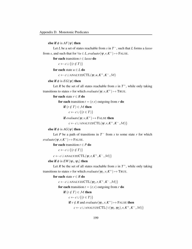
Appendix D. Monotonic Predicates
else if φ is AF(ψ) thenLet L be a set of states reachable from s in T−, such that L forms a lasso
from s, and such that for ∀u ∈ L,evaluate(ψ,r,K+) 7→ FALSE.
for each transition t ∈ lasso doc← c∪(t /∈ T )
for each state u ∈ L doc← c∪ANALYZECTL(ψ,u,K+,K−,M)
else if φ is EG(ψ) thenLet R be the set of all states reachable from s in T+, while only taking
transitions to states v for which evaluate(ψ,v,K+) 7→ TRUE.
for each state r ∈ R dofor each transition t = (r,v) outgoing from r do
if (t /∈ T ) ∈M thenc← c∪(t ∈ T )
if evaluate(ψ,v,K+) 7→ FALSE thenc← c∪ANALYZECTL(ψ,v,K+,K−,M)
else if φ is AG(ψ) thenLet P be a path of transitions in T− from s to some state r for which
evaluate(ψ,r,K+) 7→ FALSE.
for each transition t ∈ P doc← c∪(t /∈ T )
c← c∪ANALYZECTL(ψ,r,K+,K−,M)else if φ is EW (ψ1,ψ2) then
Let R be the set of all states reachable from s in T+, while only taking
transitions to states v for which evaluate(ψ1,v,K+) 7→ TRUE.
for each state r ∈ R doc← c∪ANALYZECTL(ψ2,r,K+,K−,M)for each transition t = (r,v) outgoing from r do
if (t /∈ T ) ∈M thenc← c∪(t ∈ T )if v /∈ R and evaluate(ψ1,v,K+) 7→ FALSE then
c← c∪ANALYZECTL(∨(ψ1,ψ2),v,K+,K−,M)
199
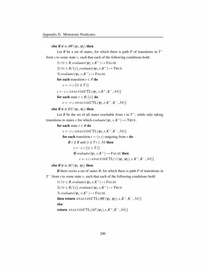
Appendix D. Monotonic Predicates
else if φ is AW (ψ1,ψ2) thenLet R be a set of states, for which there is path P of transitions in T−
from s to some state v, such that each of the following conditions hold:
1) ∀r ∈ R,evaluate(ψ2,r,K+) 7→ FALSE
2) ∀r ∈ R/v,evaluate(ψ1,r,K+) 7→ TRUE
3) evaluate(ψ1,v,K+) 7→ FALSE.
for each transition t ∈ P doc← c∪(t /∈ T )
c← c∪ANALYZECTL(ψ1,v,K+,K−,M)for each state r ∈ R/v do
c← c∪ANALYZECTL(ψ2,r,K+,K−,M)
else if φ is EU(ψ1,ψ2) thenLet R be the set of all states reachable from s in T+, while only taking
transitions to states v for which evaluate(ψ1,v,K+) 7→ TRUE.
for each state r ∈ R doc← c∪ANALYZECTL(ψ2,r,K+,K−,M)for each transition t = (r,v) outgoing from r do
if v /∈ R and (t /∈ T ) ∈M thenc← c∪(t ∈ T )if evaluate(ψ1,v,K+) 7→ FALSE then
c← c∪ANALYZECTL(∨(ψ1,ψ2),v,K+,K−,M)
else if φ is AU(ψ1,ψ2) thenif there exists a set of states R, for which there is path P of transitions in
T− from s to some state v, such that each of the following conditions hold:
1) ∀r ∈ R,evaluate(ψ2,r,K+) 7→ FALSE
2) ∀r ∈ R/v,evaluate(ψ1,r,K+) 7→ TRUE
3) evaluate(ψ1,v,K+) 7→ FALSE.
then return ANALYZECTL(AW (ψ1,ψ2),s,K+,K−,M)elsereturn ANALYZECTL(AF(ψ2),s,K+,K−,M)
200

Appendix D. Monotonic Predicates
else if φ is ∨(ψ1,ψ2) thenc← c∪ANALYZECTL(ψ1,s,K+,K−,M)c← c∪ANALYZECTL(ψ2,s,K+,K−,M)
else if φ is ∧(ψ1,ψ2) thenif evaluate(ψ1,s,K+) 7→ FALSE and evaluate(ψ2,s,K+) 7→ FALSE then
Learn the smaller of the two conflict sets for ψ1,ψ2
c1← ANALYZECTL(ψ1,s,K+,K−,M)c2← ANALYZECTL(ψ2,s,K+,K−,M)if |c1| ≤ |c2 then
c← c∪ c1
elsec← c∪ c2
else if evaluate(ψ1,s,K+) 7→ FALSE thenc← c∪ANALYZECTL(ψ1,s,K+,K−,M)
elsec← c∪ANALYZECTL(ψ2,s,K+,K−,M)
else if φ is the negation of a property state ¬p thenc← c∪¬(p(s))
else if φ is property state p thenc← c∪(p(s))
return c
201