Prudential Saving: Evidence from a Laboratory Experiment

AJ A. Bostian Christoph Heinzel∗

This Version: June 19, 2011

Abstract

Prudence is a behavioral attitude that is broadly applicable to settings involving risk. Ithas particular importance in intertemporal choice theory, where it can be interpreted as theintensity of intertemporal substitution. Prior laboratory experiments to elicit prudence haveaddressed it in a pure-risk sense, by examining behavior in static lotteries and other gambles.It is tempting to impute these results into an intertemporal context, leveraging the fact that“risk aversion” and “elasticity of intertemporal substitution” are directly mappable underexpected utility. However, many empirical studies of intertemporal behavior suggest thatthe two ideas may be distinct. To address prudence in its intertemporal sense, we insteaddesign a small-scale laboratory experiment around a two-period consumption/savings modelin order to detect prudence via savings choices. The utility concept in this model disentanglesrisk preferences from intertemporal preferences, and suggests the type of exogenous variationto present to subjects in the experiment. The experimental design involves a “multiple pricelist” with scenarios involving income risk and interest-rate risk. In each scenario, subjectsmust choose how much of their first-period income to save for the second period. The designalso implements field-like wealth levels and real time lags to ameliorate the possibility of thedecisions being a laboratory artifact. We estimate risk and intertemporal preferences at theindividual level using a subject’s savings data and the model’s structural Euler equation. Ex-cluding outliers, the average coefficient of relative risk aversion is 2.06, the average elasticityof intertemporal substitution is 0.75, and the average coefficient of relative prudence is 3.90.These averages mask a good deal of subject-level heterogeneity, as the respective coefficientsof variation are, at a minimum, 70%.

Keywords: Prudence, precautionary savings, Kreps-Porteus, laboratory experiment, time delay

JEL classification: D90, C91, C81

∗Bostian: Department of Economics, University of Virginia. Heinzel: Toulouse School of Economics (LERNA).We wish to thank Charlie Holt for his helpful comments on the experimental design, and Christian Gollier for hisassistance with modeling refinements and the interpretation of our results. We are grateful for further commentsto Antoine Bommier, Louis Eeckhoudt, Hans Gersbach, Johannes Gierlinger, Andreas Lange, Charles Noussair,Chris Otrok, Max Rueger, Harris Schlesinger, Christian Traeger, Nicholas Treich, Marie Claire Villeval and toparticipants at seminars in Toulouse, Zurich and Rennes, at the 2010 Southern Economic Association meeting,the 2011 Doctoral Meeting at Montpellier, the 2011 Econometric Society European Meeting, and the 2011 European

Group of Risk and Insurance Economists seminar where this paper was nominated for the SCOR-EGRIE YoungEconomist Best Paper Award. This research was supported by the European Research Council under the EuropeanCommunity’s Seventh Framework Programme (FP7/2007-2013) Grant Agreement no. 230589.

1

1 Overview

Kimball (1990) introduced the term “prudence” to describe the effect of a positive third derivative

of a utility function on a risky decision. Intuitively, prudence measures the sensitivity of a choice

to risk. To quantify this sensitivity, Kimball derived coefficients of absolute and relative prudence

that are analogous to the Arrow-Pratt coefficients of risk aversion. The prudence coefficients

involve derivatives of the marginal utility function (i.e., u′′′ and u′′) instead of derivatives of the

utility function. While the notion of risk aversion (as the propensity to avoid risky situations

altogether) is emprically well-established, the extent to which people are prudent is currently an

open question. In this paper, we approach this question by collecting savings data in a laboratory

context and estimating a structural Euler equation with these data.

Our approach requires us to simultaneously assess prudence in the risk and time domains. The

theoretical literature on prudence largely studies its effect on each domain independently. The

intertemporal line of research stresses the importance of a positive third derivative for capturing

reasonable precautionary-savings motives (cf. Dreze and Modigliani 1972, Leland 1968, Sandmo

1970). Indeed, precautionary savings is a paradigmatic example of prudence discussed by Kimball.

The static-risk line of research emphasizes the equivalence between a positive third derivative

and aversion to downside risks (cf. Menezes et al. 1980). There has been little examination of

whether “coefficients of prudence” are transferrable between these domains.1 The transferrability

question is of the essence when constructing an empirical strategy for estimating prudence when

both intertemporal and risk components are present.

The literature on risk aversion contains many indications that “coefficients of risk aversion” are

not transferrable between the static-risk context (e.g., decisions involving gambling and insurance)

and time (e.g., decisions involving savings and long-term investment), even though the elasticity

of intertemporal subsitution can be mathematically represented as the inverse of relative risk

aversion in many cases. For example, an oft-cited macroeconomic study by Hall (1988) finds

elasticities of intertemporal substitution near 0, which are generally incompatible with estimates

1Kimball’s derivation of prudence relies on the general insight that the convexity of marginal utility with respectto a random variable is decisive for an individual’s optimal choice of a control variable (Rothschild and Stiglitz1971). Because no assumptions are made about the context of the choice problem, the coefficients of prudence bythemselves carry no empirical context.

2

of risk aversion.2 A similarly classic laboratory experiment involving static risk by Holt and Laury

(2002) finds increasing relative risk aversion, which would generate odd predictions if applied to

many intertemporal-choice problems.3

It is likely that any discrepancies in risk aversion will also translate into discrepancies in pru-

dence, since both make use of the marginal utility function. To address this issue, we operationalize

the preference specification of Kreps and Porteus (1978) and Selden (1978) (hereafter SKP) in our

analysis. SKP provide a choice-theoretic framework that separates risk and intertemporal atti-

tudes. Kimball and Weil (2009) (hereafter KW) re-evaluate the coefficients of prudence with SKP

preferences. KW show that choice sensitivity to intertemporal risks can arise from both the risk

domain and the intertemporal domain, making SKP prudence substantially more complex than a

third derivative in either dimension. KW prudence instead involves an interaction between risk

aversion, risk tolerance, and the elasticity of intertemporal substitution.

Epstein and Zin (1989, 1991) and Weil (1990) operationalize SKP preferences in an empirical

macroeconomic context by restricting the risk domain to constant relative risk aversion and the

intertemporal domain to constant elasticity of intertemporal substitution. To our knowledge,

no empirical analysis has allowed additional flexibility in each domain’s attitudes, or measured

prudence in the joint intertemporal and risk contexts at an individual level. In this paper, we

present a new experimental design and associated econometric strategy to investigate KW prudence

within individual subjects. Our method has three components:

1. Our theoretical starting point is a two-period consumption/savings model with SKP pref-

erences used in lieu of expected utility. The theoretical interaction between risk, time, and

SKP preferences allows us to investigate potential savings responses to variations in the ex-

ogenous variables (i.e., risks, time lags, and income levels). We use these results to construct

a set of scenarios that could potentially identify prudence in a structural estimation of the

2Hall’s methodology has been critiqued on various theoretical, econometric, and data grounds. Other studies havefound evidence for positive elasticity (cf. Patterson and Pesaran 1992, Beaudry and van Wincoop 1996, Biedermanand Goenner 2008).

3If an individual exhibits increasing relative risk aversion in an intertemporal problem, his or her implicit elasticityof intertemporal substitution approaches 0 as the intertemporal utility-generating quantity (e.g., consumption)increases. In such a case, the intertemporal consumption ratio would not change with increasing wealth, a featuresomewhat difficult to reconcile with empirical evidence (see the previous footnote).

3

model, assuming the savings responses are sufficiently consistent with the model.

2. The experimental design implements these scenarios, which involve risk and a real time lag.

The presence of both risk and intertemporal elements activates both components of subjects’

decision-making.

3. Using each subject’s savings data, we estimate the structural Euler equation associated

with the model. We use a flexible yet parsimonious formulation of SKP preferences, which

allows subjects to have constant, increasing, or decreasing risk aversion, as well as constant,

increasing, or decreasing elasticity of intertemporal substitution.

This “structural-experimental” approach to analyzing savings behavior has a few advantages. First,

our behavioral tasks are grounded in a theoretical context that has been quite extensively studied.

Second, we can choose experimental scenarios that give us some reasonable a priori expectation

of obtaining prudent behavior from subjects, if it exists. In other words, we can choose exogenous

variation that will be helpful in identifying our behavior of interest. Third, because the savings

data are so completely rooted in the theoretical model, we can use the model and data to estimate

SKP preferences. With subject-level preferences in hand, we can then classify individuals along

their risk and intertemporal attitudes.

This approach does involve one important tradeoff: we must assume the existence of KW

prudence from the start. Concerns about the appropriateness of this assumption are not entirely

unwarranted; for example, in a laboratory experiment involving only the risk domain, Deck and

Schlesinger (2010) find that some subjects exhibit imprudence. However, the underlying con-

sumption/savings model is not well-behaved under imprudence – precautionary savings motives

disappear. Indeed, much of the theoretical literature on intertemporal choice notes exactly this

point, showing prudence to be a prerequisite to many stylized empirical facts (e.g., the existence

of consumption smoothing). As a result, we are inclined to let the existence of imprudence remain

an open empirical question, and operate under the assumption that prudence exists. Indeed, if

our approach fails due to the presence of imprudence, it will be immediately obvious as a failure

to identify reasonable estimates of the preference parameters.

4

A critical element in this process is the experimental design that provides our savings data.

Because we are trying to separately identify risk and intertemporal preferences, it is important to

activate both components of the decision mechanism. To address the intertemporal component, we

conduct the experiment in two stages, corresponding to the two periods in the theoretical model.

In the first stage, subjects are presented with a list of scenarios involving a first-stage income, a

second-stage income, and a second-stage interest rate. Either the second-stage income or interest

rate of each scenario is risky. Subjects can save some of the first-stage income in each scenario,

and any savings earn interest in the second stage. The savings amounts are open-ended, the only

restriction being satisfaction of the budget constraint. After a subject enters savings amounts for

all scenarios, two are randomly chosen for payment. Subjects are immediately paid the first-stage

income less savings for their two scenarios. After a real time lag of at least a few days, subjects

return for the second stage, in which the risky elements of the two scenarios are revealed. The

second-stage payment, which involves the second-stage income plus savings with interest from both

scenarios, is made immediately thereafter.

We address the risk component by altering the riskiness of the second-stage income and interest

rate. Also, to ameliorate a Rabin (2000)-style calibration critique, we scale the income levels quite

broadly, from the tens to hundreds of USD. Indeed, Holt and Laury (2002) show that risk attitudes

can change substantially with the scale of gambles, so it is potentially quite important to generate

data from both low and high scalings in order to get a reasonable calibration of preferences in the

risk domain.

Because we have relatively little a priori knowledge of how well the parameters in the risk

and intertemporal domains are identified from savings data, we conduct four small sessions of

our experiment with a variety of time lags and wealth scalings. Because of this variation, our

experiment should probably be viewed as a pilot or small-sample study of prudence attitudes.

But even with these limited data, we can provide some general typings of risk and intertemporal

characteristics, as a proof-of-concept of the analytical strategy. Indeed, we find that subjects tend

to be quite heterogeneous in their risk attitudes.

The estimation step of our analysis revealed a rather surprising empirical regularity: a subject’s

5

non-laboratory background consumption level appears to be essential for understanding his or her

savings decisions in the experiment. Failing to incorporate any background consumption causes

the model to fit very poorly for every subject. Fortunately, our theoretical framework is robust to

the inclusion of background consumption, so this result does not immediately invalidate our choice

of scenarios. It does, however, indicate that economic forces external to the laboratory setting

affected subjects’ decisions within the laboratory.

In our opinion, this spillover is probably caused by an interplay between our subject pool and

the payoff scale. Subjects were undergraduate students for whom a few hundred USD spread over

a few weeks represented a significant increase in consumption. (The financial aid office of the

associated university estimates that an average undergraduate spends about USD 1600 per month

in consumption-like expenditures.) Hence, our experiment provided a relatively large, unexpected

shock to their consumption possibilities set, one that likely brought a real consumption-smoothing

element into the laboratory savings decisions. The fact that the experimental decisions were not

“compartmentalized” within the laboratory is not particularly troubling, because these savings

decisions more closely reflect the behavior of ultimate interest. It does, however, mean that we

need to be careful about surveying subjects extensively about their consumption behavior. This

is a design feature that we did not originally anticipate, and our ability to address it ex post is

limited. We provide some robustness checks to verify the degree of bias.

The remainder of this paper is structured as follows. In Section 2, we discuss some related

empirical and experimental research. In Section 3, we present the consumption/savings model,

and show how prudential predictions are affected by introducing SKP preferences. We describe

the experimental design and econometric results in Section 4, and comment on their implications

for our understanding of prudence in Section 6. Instructions for the experiment can be found in

Appendix A.

2 Related Literature

Many intuitive theoretical results in a variety of fields in economics rely on the presence of prudence.

These include support for the concavity of the consumption function (Carroll and Kimball 1996,

6

2001), the effect of background risk on mitigating risk-taking behavior (Eeckhoudt et al. 1996,

Gollier and Pratt 1996), the relationship of optimal taxation and insurance under precautionary

labor supply (Anderberg and Andersson 2003, Low and Maldoom 2004, Netzer and Scheuer 2007),

strategic behavior in uncertain environments such as auctions, pollution problems, and rent-seeking

games (Eso and White 2004, Bramoulle and Treich 2009, Treich 2010), the hedging demand for

assets under return predictability (Gollier 2008), and the term structure of interest rates (Gollier

2010). Welfare analysis in intertemporal settings also relies on prudence: decreasing relative risk

aversion – arising when relative prudence is sufficiently stronger than relative risk aversion – causes

the “social” discount rate to decline over time (Gollier 2002a,b),4 giving relatively higher weight

to longer-term outcomes over shorter-term ones.

In contrast to these theoretical riches, the empirical evidence for prudence is remarkably incon-

clusive. Dynan (1993) uses a second-order Taylor approximation of an Euler equation to estimate

relative prudence from US consumption data, and finds a negligible coefficient of relative prudence.5

Using varied methodologies and datasets, higher but mutually inconsistent estimates have been

found (Kuehlwein 1991, Merrigan and Normandin 1996, Eisenhauer 2000, Ventura and Eisenhauer

2006). Bostian and Heinzel (2010) provide parametric structural estimates of prudence coefficients

using a flexible utility specification similar to the one in this paper. Estimating a dynamic stochas-

tic general equilibrium model on US macroeconomic data, they find evidence for decreasing relative

risk aversion and decreasing relative prudence, although the magnitudes of the declines are small.

Laboratory experiments evaluating prudence have all used its risk definition, i.e., along the

lines of Menezes et al. (1980) and Eeckhoudt and Schlesinger (2006).6 In a variant of the Holt and

Laury (2002) lottery-choice design, Tarazona-Gomez (2007) presents subjects with a list of binary

4The social discount rate is equivalent to the inverse of the expected stochastic discount factor, a ubiquitouselement of intertemporal decision-making.

5Under power utility, the coefficient of relative prudence is −u′′′ (x)x/u′′ (x) = 1+ρ, where ρ is the coefficient ofrelative risk aversion and the inverse of the elasticity of intertemporal substitution. With this specification, Dynanestimates relative prudence to be between 0.14 and 0.16, a range inconsistent with most structural macroeconomicestimates of ρ (usually between 1 and 4, cf. Meyer and Meyer 2005). Lee and Sawada (2007) re-estimate Dynan’smodel under the assumption of liquidity constraints and find relative prudence to be between 0.838 and 1.094, asubstantially higher estimate that is still incompatible with empirical estimates. These conflicting results illustratethat econometric tests of prudence can potentially be susceptible to specification error.

6Eeckhoudt and Schlesinger very generally define prudence as a preference for associating two untoward events– a sure loss of wealth and an additional independent zero-mean risk – to two different random events, instead of tojust one of them. This definition does not rely on any particular choice-theoretic framework, but does correspondto Menezes et al.’s aversion to downside risk in the expected-utility context.

7

choices between a lottery and a certain payoff. A subject’s decisions generate variation in the

revealed certainty equivalents, allowing coefficients of risk aversion and prudence to be identified.

Deck and Schlesinger (2010) also use lottery choices to test the “risk apportionment” predictions of

Eeckhoudt and Schlesinger. In each task, subjects face a lottery with two equiprobable outcomes

and must allocate their endowment between a sure gain and a lottery. Because the Eeckhoudt

and Schlesinger predictions are minimally restrictive on preferences, their associated findings are

primarily qualitative.

Ebert and Wiesen (2011) criticize both of these studies for testing preferences that are more

restrictive than those specified by the risk-apportionment theory. In the Tarazona-Gomez design,

the coefficients of prudence are derived from “truncated expected utility,” in the sense that they

come from a third-order Taylor approximation of the utility function. Because Tarazona-Gomez

only compares lotteries with equal means and variances, a test for prudence in that design collapses

to a test for skewness-seeking. By construction of their apportionment tasks, Deck and Schlesinger

also test only for skewness-seeking. Ebert and Wiesen instead compare decisions in lotteries

that vary only skewness to decisions in lotteries that implement a broader styling of risks. They

conclude that evaluating the prevalence of skewness-seeking is not sufficient to draw comprehensive

conclusions about prudence.

It is important to note that none of these experiments implement a savings context or any

other intertemporal aspect in their designs. Because risk and intertemporal attitudes may operate

separately, this lack of an intertemporal context can potentially confound the translation of their

results into intertemporal choice.

A few laboratory studies on intertemporal choice have used real time delays in conjunction

with tasks involving risk. In an artefactual field experiment, Andersen et al. (2008) show that

simultaneously eliciting risk and time preferences from the same subjects generates more coherent

estimates than distinct elicitation. The authors focus on two subject-level parameters: the coef-

ficient of relative risk aversion and the utility discount rate. In the design, data on risk attitudes

and time preferences are collected successively via two different “multiple price lists.” The first

list involves tasks that involve some risk and are immediately rewarded, and the second involves

8

tasks that involve no risk and are rewarded after some months. With an appeal to the dual-selves

model of choice (cf. Benhabib and Bisin 2005, Fudenberg and Levine 2006), the authors argue that

the responses to first set of tasks are probably temptation-driven, while the responses to latter set

are probably self-controlled. If so, then two different behaviors (risk aversion and discounting) are

revealed in the responses to each list.

Like Andersen et al., our design also emphasizes the importance of simultaneously collecting

data on risk and intertemporal attitudes from the same subject, but we do so without recourse to

dual-selves. Instead, we present subjects with one “multiple price list” of scenarios, each containing

future risk and a time delay. Our strategy is to sample a subject’s “savings function” in several

different locations via these scenarios, and then to estimate his or her savings function using the

choice-theoretic structure underlying them. This process yields joint estimates of the subject’s

risk and intertemporal preferences. And, by judiciously choosing the variation in scenarios, we can

potentially recover the higher-order risk and time preferences implicit in these estimates.7

A recent study by Andreoni and Sprenger (2009b), also unrelated to prudence, calls for addi-

tional caution when analyzing choices made in an intertemporal context. In their “convex time

budgets” design (Andreoni and Sprenger 2009a), subjects are asked to allocate a budget of ex-

perimental tokens to sooner and later payments. The two payments are either both certain, both

uncertain, or a mixture of certain and uncertain. While an expected-utility model fits the cases

where payments are uniformly certain or uncertain, the mixed case reveals a strong preference for

certainty. A certainty preference violates the continuity-in-probability assumption between certain

and uncertain outcomes of expected utility, and is also at odds with alternative models (e.g., prob-

ability weighting under prospect theory). The authors conclude that a distinction is to be made

between utility over certain consumption and utility over uncertain consumption. As shown below,

an SKP decision-maker first weights an uncertain outcome by its certainty equivalent, and then

assigns utility to the certainty-equivalent ranking. This could address the preference for certainty

found by Andreoni and Sprenger, because cases without risk (i.e., in which the certainty equivalent

is the outcome itself) will tend to be ranked higher.

7From an econometric point of view, the experiment allows us to control exogenous variation in the scenariosthat potentially heighten our ability to identify these higher-order attitudes.

9

3 The Two-Period Consumption/Savings Model

Consider a two-period consumption/savings model in which an agent receives an exogenous en-

dowment income in each period.8 The first period’s income can be split between consumption in

the first period and savings for the second period. Any amount saved earns a return in the second

period. In the von Neumann-Morgenstern (vNM) framework, this model is frequently defined in

terms of an additively-separable utility objective and two resource constraints:

U (c1, c2) = u (c1) + βE1 [v (c2)] (1)

y1 = c1 + s1 (2)

y2 + s1 (1 + r) = c2 (3)

In this formulation, u represents the agent’s first-period felicity function, v the second-period

felicity function, yt the period-t income, ct the period-t consumption, and s1 the first-period savings.

From the perspective of the first period, the second period’s felicity is discounted by the factor

β. Risk can enter from the second-period endowment y2 and the return r. We denote a scenario

θ = (y1, y2, r) as a parametrization of the exogenous elements of the agent’s problem, which includes

the applicable probability densities.

Maximizing U with respect to the savings amount s1 yields the familiar Euler condition9

E1

[βv′ (c2)

u′ (c1)(1 + r)

]= 1. (4)

Equation (4) implies that, in equilibrium, the expected discounted net return to savings must be

0%. If this return were greater than 0%, the agent could achieve higher total expected utility by

consuming relatively more in the second period (i.e., by saving relatively more in the first period).

The converse holds if this return were less than 0%. For each possible state of the world, the agent

8This is the canonical model to study individual precautionary saving (e.g., Dreze and Modigliani 1972, Leland1968, Sandmo 1970, Kimball 1990).

9For expository ease, we assume interior solutions throughout. The model can be easily extended to accommodatedecisions at a boundary.

10

applies the discount

βv′ (c2)

u′ (c1)

to the future return, a quantity that depends on his or her preferences. This stochastic discount

factor determines the agent’s savings response to any combination of current values and future

risks, and thus represents the behavioral kernel of the model.

If the agent’s preferences are unknown, one strategy for empirically reconstructing them is to

calibrate equation (4) to some savings data. This would involve estimating β, u′, and v′ using the

variation in the agent’s s1 choices that arises from variations in the scenarios θ. Our approach

to evaluating individual preferences is in exactly this vein, relying on an incentivized laboratory

experiment to generate the scenarios exogenously. As noted previously, however, this expected-

utility framework isomorphizes risk and intertemporal preferences. If these are not identical in

the agent, simply calibrating equation (4) to savings data cannot provide a reliable indicator of

preferences in either domain.

To address this issue, we use the extension of this model by Kimball and Weil (2009) with

SKP preferences as a guide for designing our experiment and associated econometric strategy. The

utility objective in this case is

U (c1, c2) = u (c1) + βv(ψ−1 (E1 [ψ (c2)])

)(5)

where ψ is a vNM utility function, but u and v are not.10 In this revised model, risk attitudes

serve as means of ranking consumption paths by their risk characteristics. Here, the ranking is

provided by the certainty equivalent ψ−1 (E1 [ψ (c2)]) of future consumption. Conditional on a risk

ranking, the functions u and v isolate the preference for consumption now versus later.

The increased flexibility of SKP preferences comes at the cost of a potentially ill-behaved model,

10Rossman and Selden (1978) show that the set of axioms sufficient for the existence of (a) the ordinal functionscapturing time preference over the two periods, and (b) a complete set of second-period vNM functions for allpossible first-period choices do not imply the existence of a two-period vNM utility function. The authors provideseveral examples of risk and intertemporal preferences that cannot be represented by two-period vNM utility but arecaptured by Selden’s (1978) “ordinal certainty-equivalent” preferences. Kreps and Porteus’ (1978) axiomatizationof recursive preferences is equivalent to Selden’s in the two-period case. They show that, contrary to intertemporalvNM utility, their framework can capture a preference for the timing of the resolution of uncertainty.

11

even if the functions u, v, and ψ are each concave (Gollier 2001). The concavity of U in s now

also requires the concavity of ψ−1(s), and this occurs if the absolute risk tolerance of ψ is concave

or if the functions u and v are linear. Otherwise, the problem’s first-order condition may yield a

local minimum. Our preference specification will ultimately obviate this issue, so for expository

purposes, we assume that u, v and ψ are strictly increasing and strictly concave, and that absolute

risk tolerance is strictly concave.

Under SKP preferences, the Euler equation involves a more complex interaction between u, v,

and ψ. Writing it in a form akin to equation (4) yields

E1

[βv′ (ψ−1 (E1 [ψ (c2)])) · ψ

−1′ (E1 [ψ (c2)]) · ψ′ (c2)

u′ (c1)(1 + r)

]= 1. (6)

The new stochastic discount factor contains effects arising from both the risk and intertemporal

domains. The first, represented by v′ (·), reflects the marginal change in future utility from a

marginal increase in the certainty-equivalent rank. The second, reflected in ψ−1′ (.)ψ′ (.), reflects

the marginal change in certainty-equivalent rank provided by a marginal change in savings. It is

worth noting that v′ (.) and ψ−1′ (.) are scalar-valued and not random variables, and so these scale

the stochastic discount factor by a constant multiple regardless of the realization of the random

elements. However, ψ′ (.) remains a stochastic quantity.

A more intuitive view of equation (4) can be found by grouping the intertemporal and risk

functions separately (cf. Rossman and Selden 1978):

u′ (c1)

βv′ (ψ−1 (E1 [ψ (c2)]))= E1

[ψ′ (c2)

ψ′ (ψ−1 (E1 [ψ (c2)]))(1 + r)

]

The left-hand side is the agent’s marginal rate of substitution between current and future consump-

tion. The right-hand side is a standard asset-pricing equation, with the pricing kernel determined

by the agent’s risk attitudes. The behavior of the kernel is primarily driven by the stochastic quan-

tity ψ′ (c2); the denominator is scalar-valued and scales the pricing kernel by a uniform amount

regardless of the realization of the random elements. The agent thus settles upon an optimal sav-

ings amount s⋆1 by introspectively equating the marginal rate of intertemporal substitution with

12

the opportunity cost of savings (i.e., the risk-adjusted return to savings).

The sensitivity of s1 to risk can be measured via the precautionary premium, a quantity which

reflects the certain compensation needed to counteract the addition of risk to the marginal utility

of saving. For small risks with mean zero and vanishing variance, Kimball and Weil use the

precautionary premium to derive the following local coefficients of absolute and relative prudence

for SKP preferences:

AP (c) = ARAψ (c)

(1 +

εψ (c)

RRISv (c)

)(7)

RP (c) = RRAψ (c)

(1 +

εψ (c)

RRISv (c)

)(8)

where ARAψ(c) and RRAψ(c) are the Arrow-Pratt coefficients of absolute and relative risk aversion

associated with ψ, εψ(c) = RPψ (c)−RRAψ (c) is the elasticity of absolute risk tolerance associated

with ψ, and RRISv (c) is the relative resistance to intertemporal substitution associated with v.11

KW prudence is thus defined by a mixture of the derivatives of ψ up to degree 3, and the derivatives

of v up to degree 2. Positive KW coefficients are sufficient for a positive precautionary premium,

implying that

εψ(c) > −RRISv(c) ⇔ −tψ′′′(c)

ψ′′(c)> RRAψ(c)−RRISv(c) (9)

for local precautionary saving to occur. Note that if v and ψ exactly coincide, the original vNM

form of U arises, and equation (9) then reduces to the familiar condition ψ′′′(c) > 0.

Kimball and Weil additionally examine global conditions for prudence under SKP preferences.

A globally necessary and sufficient condition is that ψ exhibits decreasing absolute risk aversion

(Gollier 2001), which implies that εψ (c) > 0 over the entire support. A globally sufficient condition

is that ψ′ is convex and v is more concave than ψ.

To operationalize these preferences, we choose functional forms for u, v, and ψ. The nature of ψ

as a risk-preference function suggests the use of a form that can capture a variety of risk attitudes.

11RRISv (c) has the same mathematical form as the coefficient of relative risk aversion of v. But, to avoidconfusing the behavioral effects from the risk and intertemporal domains, we never use “risk” terminology inreference to v.

13

Holt and Laury (2002) show that the expo-power function of Saha (1993) can rationalize lottery-

choice decisions in an expected-utility framework over a wide range of payoffs, a feature that is

essential in our context. The expo-power function has the form

ψ (c) =1

αψ

[1− exp

(−

αψ1− ρψ

c1−ρψ)]

(10)

and nests many common risk attitudes: constant absolute risk aversion when ρψ = 0, constant

relative risk aversion as αψ → 0, increasing (decreasing) relative risk aversion for ρψ < (>) 1

and αψ > 0, and risk neutrality when ρψ = 0 and αψ → 0.12 Importantly, the degree of risk

aversion can vary with c, potentially ameliorating somewhat the Rabin (2000) critique over a

larger range of payoffs than might be possible with a more restricted form. The nature of v

as an intertemporal-preference function suggests the use of a form that can capture a variety

of intertemporal substitution patterns. We also use an expo-power function in this case, again

because it allows the elasticity of intertemporal substitution to vary with payoffs:

v (c) =1

αv

[1− exp

(−

αv1− ρv

c1−ρv)]

(11)

It is easily verified that expo-power function has derivatives with alternating sign beginning with

positive first, has concave absolute risk tolerance, and exhibits decreasing absolute risk aversion.

Hence, the consumption/savings problem is well-behaved under this specification. In addition,

except for the case ρψ = 0, this specification provides a necessary and sufficient condition for KW

prudence to exist.

The felicity function u does not appear in the KW coefficients of prudence. However, because

we will estimate v and ψ using an Euler equation that involves u, a good specification of u is still

necessary to avoid bias in these other estimates. The most restrictive option is to assign a simple

form to u, such as linear. While this may be mathematically convenient, the form may be difficult to

12The Arrow-Pratt coefficients of absolute and relative risk aversion of expo-power utility are, respectively,ARA(c) = αc−ρ + ρc−1, and RRA(c) = αc1−ρ + ρ. The combination of α 6= 0 and ρ = 1 yields a power util-ity function that involves α instead of ρ. We do not use this specification to represent power utility, because itreflects a mathematical edge case that can be alternatively represented by first setting ρ = 1 + α and then lettingα → 0.

14

rationalize. The least-restrictive option is to estimate u separately, perhaps via another expo-power

function. However, this diminishes parsimony and ignores any potential relationship between u and

v. Indeed, u and v both measure felicity over non-stochastic consumption measures. Even though

these felicities occur in two different periods, it is plausible that they are evaluated similarly. (This

is certainly a common assumption in dynamic macroeconomic models with additively-separable

utility.) Hence, we set u = v, but also provide some evidence on the viability of a separate estimate

of u.

Having fully specified the primitives of the Euler equation, we can, in principle, estimate its

preference parameters at the individual level using equation (6). We can then use the estimates of

v and ψ to generate the KW coefficients of prudence. Grouping elements in equation (6) by time

period yields

βv′(ψ−1 (E1 [ψ (c2)])

) E1 [ψ′ (c2) (1 + r)]

ψ′ (ψ−1 (E1 [ψ (c2)]))= u′ (c1)

For expository purposees, Kimball and Weil treat this equation as a supply-and-demand system

in s1, where the left-hand side reflects the agent’s future demand for savings, and the right-hand

side reflects his or her willingness to supply of savings out of current wealth.

Their intuition is also useful here for illustrating the type of data we would need to identify

the model. In particular, we see that any observed savings amount will be an intersection point

of these supply and demand curves. To identify these curves, we thus need to have data on the

savings response to several exogenous shifts in these curves. We can generate such exogenous shifts

by varying the scenarios presented to subjects during the experiment. We have three channels of

variation at our disposal:

• the type of uncertainty subjects encounter (i.e., in future income or return),

• the probabilities associated with these random events, and

• the payoff level.

In addition, we can construct these shifts in a manner beneficial to identifying prudence using

the results of Eeckhoudt and Schlesinger (2008). There, the authors provide some necessary and

sufficient conditions for savings to increase in response to changes in risk when vNM utility is used

15

in this two-period model. We provide a similar set of conditions below for SKP preferences. For

the reader who does not wish to peruse the whole of these proofs, we highlight the following main

results:

• Corollaries 1 and 2 provide insight into the types of savings patterns that ought to be observed

under different types of uncertain events. Decisions over income gambles can help to identify

the sign of the derivatives of v, and decisions over interest-rate gambles can help to identify

a range for the coefficients of prudence v. Variation in mean-preserving spreads of these

gambles can locally identify v′′′, and variation in downside risks can identify the local rate of

change of v′′′.

• Proposition 3 shows that these variations in scenarios can also identify ψ. The return gambles

provide a particularly clean, linearly-separable substitution effect arising solely from the risk

preference. Hence, variation in savings rates in these scenarios can potentially provide a

relatively clear separation of risk attitudes and intertemporal attitudes, particularly if the

latter are also strongly identified by income gambles.

Even with these helpful theoretical identification results in hand, it is not immediately obvious

how to empirically identify v and ψ. For example, it is not clear how many scenarios should be

presented, or what range of payoffs should be used, or how much of a time lag should occur between

periods 1 and 2. These design elements will be explored further via the experimental sessions.

3.1 Comparative Statics with Changes in Income and Return Risk

By studying comparative statics of the savings decision with respect to income and return risk, we

can derive some statements about the savings patterns that ought to be observed in this two-period

setting under each type of scenario. Eeckhoudt and Schlesinger (2008) perform such an analysis

under the assumption of vNM utility; we proceed in a similar fashion under the assumption of

SKP preferences. Importantly, the results of these comparative statics depend upon the source

of the risk, and are generally different from conditions that arise from the simple addition of risk

to certainty (as in Kimball and Weil’s analysis). Eeckhoudt and Schlesinger make frequent use of

16

“increases in N th-degree risk” between two gambles (Ekern 1980). This definition of an increase in

risk requires (a) that moments 1, . . . , N − 1 be identical in both gambles, and (b) that one gamble

stochastically dominate the other via N th-order stochastic dominance (NSD). A mean-preserving

spread is an example of second-degree increase in risk, while an increase in downside risk is an

example of a third-degree increase.

Risk can enter our model from either the second-period income or the second-period return.

Recall that the first-order condition is

U ′ (s) = −u′ (y1 − s) + βv′(.)E1

[ψ′

(y2 + sR

)R]

ψ′

(ψ−1

(E1

[ψ(y2 + sR

)])) = 0 (12)

where R ≡ 1 + r is the gross return. Given our prior assumptions about strict concavity of u, v,

ψ, and the absolute risk tolerance of ψ, the second-order condition

U ′′ (s) = u′′ (y1 − s) + βv′′ (.)

E1

[ψ′

(y2 + sR

)R]

ψ′

(ψ−1

(E1

[ψ(y2 + sR

)]))

2

< 0 (13)

ensures that condition (12) has a unique solution for s. The solution is positive for positive expected

(net) returns, which we assume to hold. The following equivalence statement will be important in

following proofs.13

Definition 1 NSD equivalence ( cf. Eeckhoudt and Schlesinger): Given two random variables

zi, i = a, b, the following two statements are equivalent.

1. (i) za dominates zb via NSD.

2. (ii) Ef(za) ≤ Ef(zb) for any arbitrary function f such that sgn(f (n)(t)

)= (−1)n for all

n = 1, 2, . . . , N .

Let s∗y2,i denote the optimal solution to equation (12) when the return r is certain and second-

period income is y2 = y2,i for i = a, b. Associate in the NSD equivalence zi with second-period

13Where unambiguous, we will also use the notation f (n)(t) ≡ ∂nf(t)∂tn

in this section.

17

income y2,i and function f with v′ (ψ−1 (E1ψ(t))). Then, according to the NSD equivalence,

s∗y2,b ≥ s∗y2,a ⇔d

dsv(ψ−1 (E1ψ(y2,b + sR))

)≥

d

dsv(ψ−1 (E1ψ(y2,a + sR))

)(14)

if sgn(dn+1v(.)dsn+1

)= (−1)n for all n = 1, 2, . . . , N . The following proposition summarizes this result.

Proposition 1 Let s∗y2,i denote the optimal solution to equation (12) for a sure return r and risky

second-period income y2 = y2,i for i = a, b. The following two statements are equivalent.

1. s∗y2,b ≥ s∗y2,a, if sgn[v(n) (ψ−1 (E1ψ(t)))

]= (−1)n+1 for all n = 1, 2, . . . , N + 1.

2. y2,a dominates y2,b via NSD.

Note that Proposition 1 only provides necessary and sufficient conditions for higher optimal saving

to occur in the face of a given stochastic-dominance relationship between alternative second-period

incomes. It does not predicate the signs of the derivatives of v. Using Ekern’s definition of an

increase in N th-degree risk, the conditions of Proposition 1 simplify as follows.

Corollary 1 Let s∗y2,i denote the optimal solution to equation (12) for a sure return r and risky

second-period income y2 = y2,i for i = a, b. The following two statements are equivalent.

1. s∗y2,b ≥ s∗y2,a if sgn[v(N+1) (ψ−1 (E1ψ(t)))

]= (−1)N .

2. y2,b is an Nth-degree increase in risk over y2,a.

Statement 1 in Proposition 1 and Corollary 1 are analogous to Eeckhoudt and Schlesinger’s re-

spective conditions on marginal expected utility, but here involve the first derivative of ψ in the

risk-preference adjusted returnE1[ψ′(.)R]

ψ′(ψ−1(E1[ψ(.)]))and at least one higher derivative of v. While the

corollary only contains the sign condition for n = N + 1, the proposition holds for any N sign

conditions on v(n)(.) for all n = 1, 2, . . . , N + 1. Given thatE1[ψ′(.)R]

ψ′(ψ−1(E1[ψ(.)]))> 0, the conditions

prescribe only sign properties of the derivatives of v, and do not include higher derivatives of ψ,

in contrast to the KW coefficients of prudence.

18

The necessary and sufficient conditions for changes in return risk to increase optimal saving

are more complicated, due to the endogeneity of the riskiness of second-period consumption and

the savings choice.14

Proposition 2 Let s∗Ri denote the optimal solution to equation (12) for a sure second-period in-

come y2 and risky gross return Ri for i = a, b. The following two statements are equivalent.

1. s∗Rb ≥ s∗Ra if −s · v(n+1)(.)

v(n)(.)·

E1[ψ′(.)R]ψ′(ψ−1(E1[ψ(.)]))

≥ n for all n = 1, 2, . . . , N .

2. Ra dominates Rb via NSD.

Proof. Note that condition (14) holds analogously for any sure second-period endowment in-

come y2 and risky gross return R = Ri, i = a, b, if function h(R) ≡ v′(.)E1[ψ′(.)R]

ψ′(ψ−1(E1[ψ(.)]))satisfies

sgn(h(n)(R)

)= (−1)n for all n = 1, 2, . . . , N . For induction, consider first N = 1. With

∂v′(.)

∂R= sv′′(.) and ∂

∂R

E1[ψ′(.)R]ψ′(ψ−1(E1[ψ(.)]))

= 1, h′(R) = sv′′(.)E1[ψ′(.)R]

ψ′(ψ−1(E1[ψ(.)]))+ v′(.), so that h′(R) ≤ 0

is equivalent to −sv′′(.)v′(.)

E1[ψ′(.)R]ψ′(ψ−1(E1[ψ(.)]))

≥ 1 for v′(.) > 0. From standard induction arguments, the

following formula derives for any n > 1: h(n)(R) = snv(n+1)(.)E1[ψ′(.)R]

ψ′(ψ−1(E1[ψ(.)]))+nsn−1v(n)(.). Propo-

sition 2 then follows as in Eeckhoudt and Schlesinger (2008: 1334).

Again, Ekern’s definition of risk simplifies the conditions of Proposition 2.

Corollary 2 Let s∗Ri denote the optimal solution to equation (12) for a sure second-period income

y2 and risky gross return Ri for i = a, b. The following two statements are equivalent.

1. s∗Rb ≥ s∗Ra if −s · v(N+1)(.)

v(N)(.)·

E1[ψ′(.)R]ψ′(ψ−1(E1[ψ(.)]))

≥ N .

2. Rb is an Nth-degree increase in risk over Ra.

Statement 1 in Proposition 2 and Corollary 2 are close analogs to the respective conditions in

Eeckhoudt and Schlesinger. Thus, under both expected utility and SKP, the conditions involve

expressions that resemble coefficients of relative N th-degree risk aversion or relative N th-degree

resistance to intertemporal substitution, only for the case of y2 = 0 (as assumed by Eeckhoudt and

14Selden (1979) studies savings behavior under return risk using his type of recursive preferences. Langlais (1995)treats the case of N = 2, as does Weil (1990) for generalized isoelastic preferences.

19

Schlesinger).15 As in the case of risky second-period income and sure return, the conditions only

involve the first derivative of ψ and particularly depend on the sign properties of the derivatives

of v.

To see how the two settings generate different savings behavior, consider an increase in second-

order risk (N = 2) in each variable. When the increase arises from second-period income, precau-

tionary saving will increase if the agent is prudent with respect to v. However, when the increase

arises from the second-period return, two effects arise as Eeckhoudt and Schlesinger note, which

can be observed via the equation

h′′(R) = s2v′′′(.)E1

[ψ′(.)R

]

ψ′ (ψ−1 (E1 [ψ (.)]))+ 2sv′′(.)

If v were quadratic with v′′ > 0 but v′′′ = 0, then h′′(R) < 0. An agent with resistance to

intertemporal substitution would save less because saving increases the second-order riskiness of

second-period consumption. This constitutes a substitution effect of current consumption for future

consumption. If, however, the consumer is prudent with respect to v, then the additional second-

order risk on second-period consumption will induce a precautionary effect. For a net increase in

savings to occur, this precautionary effect must dominate the substitution effect. This occurs if

and only if the product of optimal saving and the coefficient of prudence of v exceeds two.

Finally, the change in optimal savings for a scenario element θi is given by the implicit function

theorem:

ds∗

dθi= −

∂F (s;θ)∂θi

∂F (s;θ)∂s

|s=s∗ (15)

where F (s; θ) is defined as U ′ (s) under the scenario θ. Gollier (2001) provides sign conditions on

ds⋆/dθi under expected utility, which extend to the case of SKP preferences.16 We also provide a

15Eeckhoudt and Schlesinger refer to a quantity of the form − tu(n)(t)u(n−1)(t)

as a measure of “relative nth-degree risk

aversion” and use the established terms of risk aversion, prudence, temperance and edginess for n = 2, 3, 4, 5. Theterm “resistance to intertemporal substitution” for coefficients involving two adjacent derivatives of the intertem-poral function v is used by Kimball and Weil.

16Because ∂F (s,θ)∂s

< 0 (see equation (13)), the sign of ds∗

dθiin equation (15) is uniquely determined by the numerator

of equation (15).

20

condition summarizing the effect of adding a constant c to the consumption level in each period,

which will prove useful later.

Proposition 3 Let s∗ denote the optimal solution to equation (12). A marginal increase in an

endowment parameter changes optimal savings ceteris paribus as follows.

sgn

[ds∗

dy1

]= sgn [−u′′(.)] > 0 (16)

sgn

[ds∗

dy2

]= sgn

[v′′(.)

E1[ψ′(.)R]

ψ′ (ψ−1 (E1 [ψ (.)]))

]< 0 (17)

sgn

[ds∗

dr

]= sgn

[sv′′(.)

E1[ψ′(.)R]

ψ′ (ψ−1 (E1 [ψ (.)]))+ v′(.)

]T 0 for − s

v′′(.)

v′(.)

E1[ψ′(.)R]

ψ′ (ψ−1 (E1 [ψ (.)]))S 1

(18)

sgn

[ds∗

dc

]= sgn

[−u′′(.) + βv′′(.)

E1[ψ′(.)R]

ψ′ (ψ−1 (E1 [ψ (.)]))

]< 0 if (19)

ARA′

ψ < 0 and − v′′(.)

[v′(.)]2weakly increasing or

ARA′

ψ, AP′

ψ < 0, ARISv ≥ ARAψ, and εv +RRISv ≤ εψ +RRAψ

The sign conditions in Proposition 3 derive from straightforward calculation of all derivatives

involved. The qualification in condition (18) comes from Gollier by analogy, and the qualifications

in condition (19) stem from Kimball andWeil. As conditions (16) and (17) indicate, optimal savings

increase with y1 but decrease with y2, expressing the preference for consumption smoothing. Note

that this property solely depends on characteristics of the intertemporal utility functions u and v.

The sign of the impact of a marginal increase in the interest rate r depends on the relative strengths

of two effects. First, the prospect of being wealthier in the future permits the agent to have a

higher consumption today, smoothing consumption over time. This wealth effect is captured by

the negative first term on the right-hand side of equation (18). Second, an increase in the interest

rate gives an incentive to save more today and thus to substitute future consumption for current

consumption due to the reduction of the relative price of future consumption. This substitution

effect is expressed by the positive second term. The substitution effect dominates (is dominated

by) the wealth effect if the coefficient of relative resistance to substitution of v with respect to s

21

is smaller (larger) than 1, as can be seen by factoring out v′(.). Finally, the impact of an increase

in c is ambiguous, as it hinges on the relative strengths of the two effects stated in conditions (16)

and (17).

4 Experimental Design and Econometric Analysis

The two-period consumption/savings model and the conditions for increased saving under risk

changes of Section 3 guide our experimental design including the construction of scenarios. The

design comprises two phases, which are separated by a time delay of several days or weeks. In Phase

1, subjects are presented with a list of scenarios of endowment income y1 and a future lottery over

either Phase-2 endowment y2 or return r. In each scenario, a subject chooses the savings amount

s1 out of endowment income y1. The scenarios are presented to subjects in a manner similar to a

“multiple price list.” (An illustrative list for each of the income and interest tasks can be found in

Tables 1 and 2 below.) At the end of Phase 1, two scenarios are picked at random to be paid in full

value. Subjects are paid c1 = y1− s1 for these scenarios. In Phase 2, subjects first complete a set

of surveys lasting about as long as Phase 1.17 The surveys include the Cognitive Reflection Test,

the Big-Five Inventory personality test, and demographics. Subjects then resolve uncertainty in

y2 or r in their scenarios for payment, and are paid c2 = y2 + s1 (1 + r) for these scenarios.

Each scenario belongs to either of two classes of decision tasks which correspond to the two

types of random events in the model. In the first task class, the return is fixed at r = 20%, and risk

enters only from uncertainty in second-period income, which is centered at y1 = E1(y2) = $20. In

the second task class, incomes are fixed at y1 = y2 = $20, and risk enters only from uncertainty in

the return, which is centered at E1(r2) = 20%. The risky element of each task is a binary gamble

consisting of two prospects of the form (z; Pr(z)), where z ∈ {y2, r}. For notational convenience,

we denote zh as the higher and zl as the lower of the two outcomes, and associate π with the

probability of the higher outcome Pr(zh).

Given this setup, we construct risk changes in the scenarios that may be useful for identifying

17In a recent intertemporal design, Andreoni and Sprenger (2009b) note the importance of equalizing unobservedshadow costs of visiting the laboratory across visits (e.g., time costs).

22

Kimball-Weil prudence:

• Base case: Lz ={(zl; 1− π

),(zh; π

)}

• Mean-preserving spread: Lz ={(zl − η; 1− π

),(zh + γ; π

)}

• Increased downside risk: Lz ={(zl + ν; 1− π + δ

),(zh + µ; π − δ

)}

The two prospects in a base lottery can be altered to satisfy the appropriate risk definition. For a

mean-preserving spread, this involves subtracting η from the lower outcome and adding a constant

γ to the higher outcome, so that the new gamble has the same mean as the original. For an

increase in downside risk, this involves adding a constant δ to the lower outcome’s probability and

subtracting δ from the higher outcome’s probability, and then adding µ and ν to the high and low

outcomes, so that the original mean and variance are preserved.18

In the income tasks, savings should increase with γ if v′′′ (ψ−1 (E1ψ(c2))) ≥ 0, and with δ if

v′′′′ (ψ−1 (E1ψ(c2))) ≤ 0 (Corollary 1). In the interest-rate tasks, savings should increase with γ

if −v′′′(.)v′′(.)

· s · E1[ψ′(.)(1+r)]ψ′(.)

≥ 2, and with δ if −v′′′′(.)v′′′(.)

· s · E1[ψ′(.)(1+r)]ψ′(.)

≥ 3 (Corollary 2). Moreover,

adding income risk to a setting of certainty raises savings under KW prudence (cf. Section 3).

To assess these tendencies, the design involves, apart from a degenerate lottery, the exogenous

manipulations η ∈ {0, 4, 8, 12, 16} for π = 0.5 and π = 20/(20 − η), yielding a total of 9 savings

choices involving mean-preserving spreads. Moreover, we pick the scenarios with η ∈ {8, 16} and

π = 0.5 to construct lotteries with the exogenous manipulations δ ∈ {0.1, 0.2, 0.25, 0.3, 0.4}, for a

total of 10 savings choices involving increases in downside risk.

In addition to varying the risks and payoffs, we also vary the payoff scale. The idea that risk

attitudes can vary with the wealth level is at least as old as Pratt (1964). Rabin (2000) provides

evidence that this variation is actually empirically necessary to avoid troublesome predictions about

lottery choices at varying scales, but that such variation still leaves some puzzling predictions in the

expected-utility framework. Indeed, Holt and Laury (2002) note exactly such a wealth effect when

their lottery-choice design is conducted at substantially different payoff levels. Because prudence

can potentially vary with the income level, and because the higher income levels are more likely

18This implies that µ1,2 =(zh − zl

)(π ±

√π(1−π)1−π+δ

), and ν1,2 =

(zh − zl

) (π ±

√π(1− π) 1−π+δ

π−δ

).

23

ScenarioToday’sIncome

Tomorrow’s IncomeTomorrow’sInterest Rate

How Much toSave Today?

1 $20.00 $16.00 with probability 0.5 20% $$24.00 with probability 0.5

2 $20.00 $8.00 with probability 0.4 20% $$28.00 with probability 0.6

3 $20.00 $9.52 with probability 0.7 20% $$44.44 with probability 0.3

Table 1: Decision table for example tasks involving income lotteries, x = 1 scaling.

ScenarioToday’sIncome

Tomorrow’sIncome

Tomorrow’s Interest RateHow Much toSave Today?

1 $20.00 $20.00 16.0% with probability 0.5 $24.0% with probability 0.5

2 $20.00 $20.00 12.0% with probability 0.6 $32.0% with probability 0.4

3 $20.00 $20.00 17.3% with probability 0.9 $44.0% with probability 0.1

Table 2: Decision table for example tasks involving interest-rate lotteries, x = 1 scaling.

to reflect our behavior of interest (prudential savings), we believe it is important to collect savings

decisions at a variety of income levels. Thus, the design also involves collecting similar decisions for

payoffs scaled by factors x ∈ {1, 2.5, 5, 7.5, 10}. These lead to gambles with the same qualitative

risk characteristics, but substantially different payoffs.

To concretize the content of the list, we consider a case in which five tasks with income gambles

are always followed by five gambles with return gambles. (In the experiment, the “return” is called

an “interest rate” for clarity.) Moreover, the payoff scaling changes every five or ten tasks. The

first half of the list starts with x = 1 and then moves to x = 10 and x = 7.5, while the second half

starts again with x = 1 and moves to x = 2.5 and x = 5. Presenting decisions to subjects in a

semi-structured fashion may lead to fewer inconsistent choices than if the scenarios are presented

in a random order.19 This particular elicitation procedure generates 60 scenarios and associated

savings decisions.

19We thank Charlie Holt for this helpful suggestion.

24

4.1 Econometric Analysis

We use each subject’s savings data in order to estimate the parameters of our SKP-enhanced Euler

equation (6) at the individual level. For a particular model parametization ω = (β, αψ, ρψ, αv, ρv),

Euler equation (6) implicitly defines a unique savings amount s⋆ij (ω) for each scenario j faced

by subject i. Our econometric strategy attempts to match this prediction with the quantity sij

actually observed. In particular, we minimize the sum of squared prediction errors ηij = sij−s⋆ij (ω),

ωi = argminω

Ji∑

j=1

η2ij =

Ji∑

j=1

(sij − s⋆ij (ω)

)2

over all Ji scenarios faced by this subject. The asymptotic covariance matrix for this well-known

nonlinear least-squares estimator is σ2iη (S

′

iSi)−1, where σ2

iη is the variance of ηij and Si is the Jaco-

bian of si =(s⋆i1 (ω) , · · · , s

⋆iJi

(ω)). For each subject, we had difficulty numerically approximating

∇s⋆ij (ω) in some scenarios, making S ′

iSi generally ill-behaved and unsuitable for inversion. Hence,

we do not provide standard errors for any of our estimates. In light of the poor performance of

the asymptotic estimator, a bootstrap estimator is probably a more robust method for obtaining

the covariance of ωi.

We encountered a few identification issues when estimating this model. First, the utility dis-

count factor β is not very well identified, a result that is probably not surprising given the short

time intervals used thus far (cf. Section 5). We hence constrain β = 1 throughout, leaving us

with a four-parameter specification. Second, the model exhibited very poor fit when we defined

“consumption” entirely within the context of the experiment. The model performed much better

when we added an additional consumption quantity c in each period, so that

c1 = c+ y1 − s1

c2 = c+ y2 + (1 + r) s1

This result could be interpreted in a few ways. First, it may reflect a specification error in our

model’s structure. If true, the source of the error must closely reflect the risk and intertemporal

25

changes generated by the model via uniformly shifting consumption by c, which would be a very

peculiar kind of error. Alternatively, it could imply that subjects consider the savings problem from

a context larger than the laboratory, so that c reflects a background consumption level they either

have or anticipate having during each period. Indeed, several of the scenarios involve monetary

values that are quite high for our student cohort, and they may have seriously considered the

consumption-smoothing possibilities implied by these scenarios. If this is the correct interpretation,

then the consumption smoothing we observe is not solely generated within the laboratory; the

laboratory has spilled partially into the field. Indeed, we might be more assured that we are

estimating risk and intertemporal characteristics that are relevant to field decisions.

Importantly, our experiment still generated an unanticipated, controlled shock to subjects’

consumption possibilities set, so the responses we observe probably only reflect this exogenous

source of variation and not any field elements beyond the background consumption. In addition,

because our subject pool consists of in-session undergraduates, it is unlikely that they would have

had an opportunity to reassess their second-period background consumption as a result of the

experiment. And, the theoretical results from the previous section are impervious to the addition

of a constant c, so our scenario selection still has value for identifying prudence. However, the

comparative static exercise on initial wealth in equation (19) shows that the interpretation of the

outcomes will likely vary with c.

Thus, if our conjecture about the importance of background consumption is valid, we have an

additional question of how to empirically address c. This is not without some concern, because

it is possible to generate all manner of risk and intertemporal attitudes by arbitrarily scaling c

for given data. The best option is probably to conduct a detailed survey about subjects’ current

and anticipated consumption during the first phase of the experiment, but we unfortunately did

not anticipate this requirement for these sessions. A second option is to treat c as an estimatable

parameter, but it is not clear how the savings data would identify it. A further option is to impute a

value for c. Because our subjects were in-session undergraduate students, it is likely that they had a

relatively limited and consistent set of consumption expenditures. In addition, they were probably

most concerned about consumption over a relatively short interval. The University of Virginia

26

Session Scenarios Interval Subjects Male/Female Avg. Earnings1 30 2 days 5 1/4 $326.262 54 7 days 5 3/2 $331.083 60 14 days 5 1/4 $193.494 60 14 days 5 4/1 $280.95

Table 3: Session description.

publishes estimates of the expenditures that an undergraduate can anticipate during an academic

year,20 and we imputed a monthly consumption value by summing the total non-tuition elements

of this estimate and dividing by the number of months in a standard two-semester academic year.21

Under this method, our estimate of monthly background consumption is $1620. Finally, because

of the variation in the time intervals in different sessions, we tailored c according to the actual

interval. The final imputed values of c are $1620/15 = $108 in Session 1, $1620/4 = $405 in

Session 2, and $1620/2 = $810 in Sessions 3 and 4.

We estimated the model using the simulated annealing algorithm, a stochastic search process

that is relatively robust to the presence of local minima and nonconvexities. We began the search

at linear specifications for v and ψ, and stopped it after 10,000 random points were evaluated in

the parameter space. For most subjects, the algorithm converged upon a minimum within a few

thousand iterations, implying that our initial assumption about the existence of KW prudence is

probably safe. In three cases, it did not find an improved point. In one of these cases, the subject

always saved the all of the first-stage income; the other two exhibited small variations in savings

decisions that were probably not sufficient to identify the savings function.

5 Data and Results

Our empirical results are based on four sessions with five undergraduate subjects each that we

conducted at the Veconlab Experimental Economics Laboratory at the University of Virginia in

April and May 2010. Table 3 describes the sessions. We scheduled, when possible, the sessions so

that subjects arrived on the same day of the week on each visit, in an attempt to keep the external

20These estimates are available at http://www.virginia.edu/financialaid/estimated.php.21This total includes room, board, and various discretionary items, but not tuition and fees.

27

0

0.25

0.5

0.75

1

0 50 100 150 200

Fra

ctio

n of

End

owm

ent S

aved

Initial Endowment

Session 1Session 2Session 3Session 4

0

0.25

0.5

0.75

1

0 50 100 150 200

Fra

ctio

n of

End

owm

ent S

aved

Initial Endowment

Session 1Session 2Session 3Session 4

Figure 1: Savings rates by y1, for income tasks (left) and interest tasks (right).

0

0.25

0.5

0.75

1

0 0.25 0.5 0.75 1

Fra

ctio

n of

End

owm

ent S

aved

Pr(low outcome)

Session 1Session 2Session 3Session 4

0

0.25

0.5

0.75

1

0 0.25 0.5 0.75 1

Fra

ctio

n of

End

owm

ent S

aved

Pr(low outcome)

Session 1Session 2Session 3Session 4

Figure 2: Savings rates by 1− π, for income tasks (left) and interest tasks (right).

influence of regular wage payments constant. Because the dollar amounts paid to subjects can be

high, we ran the sessions in very quick succession (within two days) so that there would be limited

time for word-of-mouth discussion about the experiment. In the first session, we used 30 scenarios

and a lag of 2 days. These scenarios did not include any downside-risk manipulations. The second

session involved 54 scenarios with both mean-preserving spreads and downside risk increases, and

a lag of 7 days. The last two sessions used the full 60 scenarios described above and lags of 14 days

each. Average payments routinely exceeded $200, because subjects in this small sample received

favorable draws of the random elements.

Figure 1 plots the average savings rates in these sessions by initial endowment, and Figure 2

plots them by probability of the low outcome in the lottery. On average, subjects appear to save

a good deal: average savings rates are always above 50%. Interestingly, subjects appear to be

28

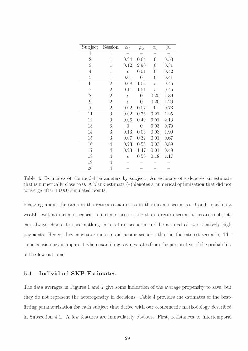
Subject Session αψ ρψ αv ρv1 1 – – – –2 1 0.24 0.64 0 0.503 1 0.12 2.90 0 0.314 1 ǫ 0.01 0 0.425 1 0.01 0 0 0.416 2 0.08 1.03 ǫ 0.457 2 0.11 1.51 ǫ 0.458 2 ǫ 0 0.25 1.399 2 ǫ 0 0.20 1.2610 2 0.02 0.07 0 0.7311 3 0.02 0.76 0.21 1.2512 3 0.06 0.40 0.01 2.1313 3 0 0 0.03 0.7014 3 0.13 0.03 0.03 1.9915 3 0.07 0.32 0.01 0.6716 4 0.23 0.58 0.03 0.8917 4 0.23 1.47 0.01 0.4918 4 ǫ 0.59 0.18 1.1719 4 – – – –20 4 – – – –

Table 4: Estimates of the model parameters by subject. An estimate of ǫ denotes an estimatethat is numerically close to 0. A blank estimate (–) denotes a numerical optimization that did notconverge after 10,000 simulated points.

behaving about the same in the return scenarios as in the income scenarios. Conditional on a

wealth level, an income scenario is in some sense riskier than a return scenario, because subjects

can always choose to save nothing in a return scenario and be assured of two relatively high

payments. Hence, they may save more in an income scenario than in the interest scenario. The

same consistency is apparent when examining savings rates from the perspective of the probability

of the low outcome.

5.1 Individual SKP Estimates

The data averages in Figures 1 and 2 give some indication of the average propensity to save, but

they do not represent the heterogeneity in decisions. Table 4 provides the estimates of the best-

fitting parametrization for each subject that derive with our econometric methodology described

in Subsection 4.1. A few features are immediately obvious. First, resistances to intertemporal

29

Sessions 1-4 Increasing RRA Decreasing RRA Constant RRA CountIncreasing RRIS 2 1 3Decreasing RRIS 3 4 7Constant RRIS 2 3 2 7

Count 7 4 6 17

Sessions 3 & 4 Increasing RRA Decreasing RRA Constant RRA CountIncreasing RRIS 2 1 3Decreasing RRIS 3 2 5Constant RRIS

Count 5 1 2 8

Table 5: Breakdown of relative risk aversion and relative resistance to intertemporal substitution.

substitution in Sessions 1 and 2 appear to be usually constant and smaller in magnitude than in

Sessions 3 and 4. This could imply that the time delay was not sufficiently long in the first two

sessions to create a meaningful intertemporal tradeoff. (In other words, the two stages may not

have corresponded to separate evaluation periods.) In addition, subjects in Sessions 1 and 2 also

tend to have lower levels of risk aversion, with quite a few instances of risk neutrality. These initial

sessions did not involve as many scenarios and may not adequately generate enough variation for

estimating risk attitudes either.

The breakdown for RRA and RRIS in our experimental cohort are provided in Table 5. Cases

that did not exhibit model convergence are omitted from the breakdown, and ǫ values are treated

as 0. In the full cohort, 18% of subjects exhibited IRRIS, 41% exhibited DRRIS, and 41% exhibited

CRRIS. In addition, 41% exhibited IRRA, 24% exhibited DRRA, and 35% exhibited CRRA. This

picture, however, changes substantially for Sessions 3 and 4. Across this sub-sample, 38% exhibit

IRRIS, 62% exhibit DRRIS, and 0% exhibit CRRIS. And, 62% exhibit IRRA, 13% exhibit DRRA,

and 25% exhibit CRRA. The shifts of frequency (a) away from CRRIS and (b) towards IRRA

strongly suggest that Sessions 3 and 4 are generating different behavior. Of course, this result

occurs in a small sample, so it is difficult to provide statistical support for this effect.

Finally, these estimates allow us to estimate the degree of prudence in our subjects. Recall

that the functional form for relative KW prudence is

RP (c) = RRAψ (c)

(1 +

εψ (c)

RRISv (c)

)= RRAψ (c)

(1 +

RPψ (c)−RRAψ (c)

RRISv (c)

)

30

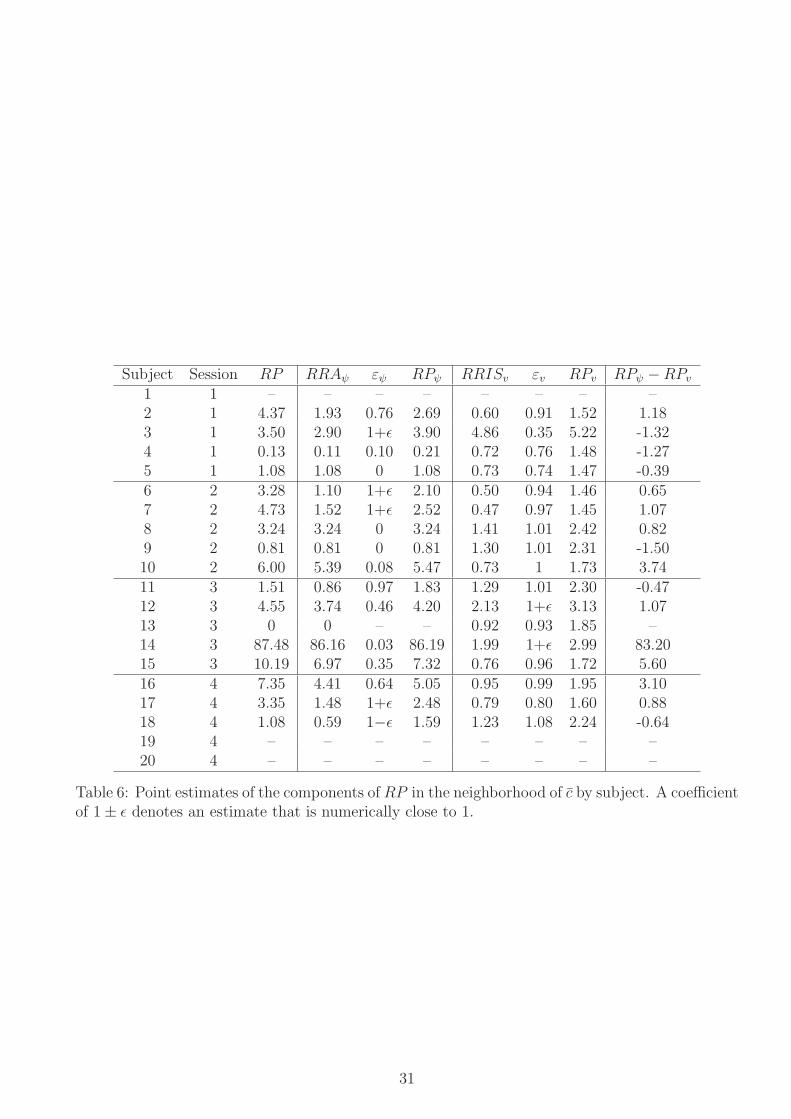
Subject Session RP RRAψ εψ RPψ RRISv εv RPv RPψ −RPv1 1 – – – – – – – –2 1 4.37 1.93 0.76 2.69 0.60 0.91 1.52 1.183 1 3.50 2.90 1+ǫ 3.90 4.86 0.35 5.22 -1.324 1 0.13 0.11 0.10 0.21 0.72 0.76 1.48 -1.275 1 1.08 1.08 0 1.08 0.73 0.74 1.47 -0.396 2 3.28 1.10 1+ǫ 2.10 0.50 0.94 1.46 0.657 2 4.73 1.52 1+ǫ 2.52 0.47 0.97 1.45 1.078 2 3.24 3.24 0 3.24 1.41 1.01 2.42 0.829 2 0.81 0.81 0 0.81 1.30 1.01 2.31 -1.5010 2 6.00 5.39 0.08 5.47 0.73 1 1.73 3.7411 3 1.51 0.86 0.97 1.83 1.29 1.01 2.30 -0.4712 3 4.55 3.74 0.46 4.20 2.13 1+ǫ 3.13 1.0713 3 0 0 – – 0.92 0.93 1.85 –14 3 87.48 86.16 0.03 86.19 1.99 1+ǫ 2.99 83.2015 3 10.19 6.97 0.35 7.32 0.76 0.96 1.72 5.6016 4 7.35 4.41 0.64 5.05 0.95 0.99 1.95 3.1017 4 3.35 1.48 1+ǫ 2.48 0.79 0.80 1.60 0.8818 4 1.08 0.59 1−ǫ 1.59 1.23 1.08 2.24 -0.6419 4 – – – – – – – –20 4 – – – – – – – –

Table 6: Point estimates of the components of RP in the neighborhood of c by subject. A coefficientof 1± ǫ denotes an estimate that is numerically close to 1.

31

implying that we need to compute RPψ, RRAψ, and RRISv.22 Table 6 presents point estimates of

relative KW prudence and its risk and intertemporal components for each subject, evaluated at the

applicable c. RRA is greater than 1 in 12 subjects (71%), and greater than 5 in 5 subjects (29%).

Subjects 13 and 14 are outliers in this cohort, one exhibiting risk-neutrality and the other extreme

risk aversion. RRIS is less than 1 in 10 subjects (59%), and greater than 1 in the remaining 7

subjects (41%). The extremes of these estimates are 0.47 and 4.86. The elasticity εψ is equal to

1 for 5 subjects (29%), and less than 1 for the remaining 12 subjects (71%). The elasticity εv is

equal to 1 for 3 subjects (17%), less than 1 for 10 subjects (59%), and greater than 1 for 4 subjects

(24%). The fact that these elasticities are not usually equal to 1 implies that the increasing or

decreasing shape of a subject’s RRA and RRIS is indeed an important component of his or her

risk and intertemporal preferences. (Recall that relative prudence is simply constant at 1 + ρ for

power utility, the case in which ε = 1.)

Table 6 also shows that risk-domain prudence is stronger than intertemporal-domain prudence

for 10 subjects (59%). The correlation coefficient for the two attitudes is 0.24, indicating a mod-

erately positive relationship between risk and intertemporal prudence in an average subject. The

estimates of KW prudence range from 0 to 87.48, and are typically less then 5 (76%).

After eliminating the two outliers, we find that the average RRA is 2.06, the average RRIS is

1.34 (implying that the elasticity of intertemporal substitution is 1/1.34 ≈ 0.75), and the average

RP is 3.90. These averages, however, mask a good deal of heterogeneity: the standard deviations

of these estimates are 1.58 for RRA, 1.27 for RRIS, and 2.82 for RP . Hence, using an average

risk attitude to generate savings amounts (e.g., via a representative-agent analysis) would yield

savings rates that many subjects would probably not prefer.

6 Discussion

Our threefold procedure for analyzing prudence in an intertemporal context – an interrelated web

of theory, experiment, and structural estimation – appears to have the ability to elicit and identify

22If subjects are risk neutral, RPψ and RRAψ are identically zero, making RP zero in that case. And, if subjectshave no resistance to intertemporal substitution, RP explodes. A few of our subjects, particularly in Sessions 1and 2, exhibit at least one of these characteristics.

32

Subject Session αψ ρψ αv ρv1 1 – – – –2 1 0.05 0.14 0.01 0.273 1 0.04 0.22 0.04 1.494 1 0.11 1.05 0.05 0.585 1 0 0 0.23 1.956 2 0.04 0.46 0 1.507 2 0.06 0.40 0.01 0.918 2 0.01 ǫ 0.01 0.529 2 0.03 0.33 0.11 0.5310 2 0.04 0.19 0.01 0.4211 3 0.04 1.87 0.09 2.2712 3 0.03 0.24 0.14 0.5813 3 0 0.28 0.02 1.5914 3 0.07 0.12 0.05 0.8515 3 0.05 0.25 0.06 1.2516 4 0.11 0.42 0.10 1.6317 4 0.03 2.46 0.03 1.0018 4 0.10 0.99 0.09 0.6419 4 – – – –20 4 – – – –

Table 7: Estimates of the model parameters by subject for c = $1620. A value of ǫ denotes anumber that is numerically close to 0.

prudence in laboratory subjects. We find estimates that are generally plausible, but exhibit a good

deal of between-subject variation.

Clearly, the weakest link in our strategy is the fact that we do not have a good grasp on

how closely the laboratory and the field are interacting within our subjects. Laboratory actions

certainly appear to incorporate some non-laboratory context, so it is essential to understand the

external factors as well. To illustrate the sensitivity of our method to this aspect of the model, we

provide alternative estimates of risk and intertemporal preferences assuming a common background

consumption level c = $1620 in Table 7. Comparing these estimates to those in Table 4 (tailored

to a session-specific c), we find that many have changed substantially. Probably the best way to

address this issue is to survey subjects about their current and estimated consumption expenditures

at the end of the first stage, and then verify these again as part of the second stage.

We also find that a time delay of a few days and perhaps even a few weeks may not activate

the desired risk and intertemporal attitudes we wish to study. This is evident in the complete

33

lack of empirical identification in the savings data of three of our subjects. Subjects may mentally

account the payments as pure windfalls when such payments are large and closely spaced, which

may not lead to the desired risk and intertemporal tradeoffs. Probably the best alteration to our

design in such a case is to increase both the risk and the time interval.

Interestingly, our study finds a way to reconcile the IRRA results of Holt and Laury (2002) with

the CRRIS or DRRIS that is frequently observed in intertemporal problems such as consumption

smoothing. Indeed, in the best parametrization of our experiment, the risk estimates appear to be

moving primarily towards IRRA, and the intertemporal estimates appear to be moving primarily

towards DRRIS. The reason, to use the words of a recent study, is that “risk preferences are not

time preferences” (Andreoni and Sprenger 2009b), and so it is possible for subjects to hold both

attitudes simultaneously.

This design could potentially be used to classify individuals according to their risk and in-

tertemporal characteristics. The empirical density of such estimates could be used in models for

which the distribution of such attitudes is important, such as those mentioned in the literature

section. Future research to refine the design and verify its consistency could provide insight into

population-level risk and intertemporal preferences.

34

References

Dan Anderberg and Fredrik Andersson. Investments in human capital, wage uncertainty, andpublic policy. Journal of Public Economics, 87(7–8): 1521–1537, 2003.

Steffen Andersen, Glenn W. Harrison, Morten I. Lau, and E. Elisabet Rutstrom. Eliciting Riskand Time Preferences. Econometrica, 76(3): 583–618, 2008.

James Andreoni and Charles Sprenger. Estimating Time Preferences from Convex Budgets. 2009a.University of California, San Diego, mimeo.

James Andreoni and Charles Sprenger. Risk Preferences Are Not Time Preferences. 2009b. Uni-versity of California, San Diego, mimeo.

Paul Beaudry and Eric van Wincoop. The intertemporal elasticity of substitution: An explorationusing a US panel of state data. Economica, 63(251): 495–512, 1996.

Jess Benhabib and Alberto Bisin. Modeling internal commitment mechanisms and self-control: Aneuroeconomics approach to consumption-saving decisions. Games and Economic Behavior, 52(2): 460–492, 2005.

Daniel K. Biederman and Culler F. Goenner. A life-cycle approach to the intertemporal elasticityof substitution. Journal of Macroeconomics, 30(1): 481–498, 2008.

AJ A. Bostian and Christoph Heinzel. Macroeconomic Evidence for Prudence. 2010. Universityof Virginia and Toulouse School of Economics (LERNA), mimeo.

Yann Bramoulle and Nicolas Treich. Can Uncertainty Alleviate the Commons Problem? Journalof the European Economic Association, 7(5): 1042–1067, 2009.

Christopher D. Carroll and Miles S. Kimball. On the Concavity of the Consumption Function.Econometrica, 64(4): 981–992, 1996.

Christopher D. Carroll and Miles S. Kimball. Liquidity Constraints and Precautionary Saving.2001. NBER Working Paper 8496.

Cary Deck and Harris Schlesinger. Exploring Higher Order Risk Effects. Review of EconomicStudies, 77(4): 1403–1420, 2010.

Jacques H. Dreze and Franco Modigliani. Consumption Decisions under Uncertainty. Journal ofEconomic Theory, 5(3): 308–335, 1972.

Karen E. Dynan. How Prudent Are Consumers? Journal of Political Economy, 101(6): 1104–1113,1993.

Sebastian Ebert and Daniel Wiesen. An experimental methodology testing for prudence and third-order preferences. Management Science, 57(7): 1334–1349, 2011.

Louis Eeckhoudt and Harris Schlesinger. Putting Risk in Its Proper Place. American EconomicReview, 96(1): 280–289, 2006.

Louis Eeckhoudt and Harris Schlesinger. Changes in risk and the demand for saving. Journal ofMonetary Economics, 55(7): 1329–1336, 2008.

35

Louis Eeckhoudt, Christian Gollier, and Harris Schlesinger. Changes in Background Risk and RiskTaking Behavior. Econometrica, 64(3): 683–689, 1996.

Joseph G. Eisenhauer. Estimating Prudence. Eastern Economic Journal, 24(6): 379–392, 2000.

Steinar Ekern. Increasing Nth Degree Risk. Economics Letters, 6(4): 329–333, 1980.

Larry G. Epstein and Stanley E. Zin. Substitution, Risk Aversion, and the Temporal Behaviorof Consumption and Asset Returns: A Theoretical Framework. Econometrica, 57(4): 937–969,1989.

Larry G. Epstein and Stanley E. Zin. Substitution, Risk Aversion, and the Temporal Behavior ofConsumption and Asset Returns: An Empirical Analysis. Journal of Political Economy, 99(2):263–286, 1991.

Peter Eso and Lucy White. Precautionary Bidding in Auctions. Econometrica, 72(1): 77–92, 2004.

Drew Fudenberg and David K. Levine. A Dual-Self Model of Impulse Control. American EconomicReview, 96(5): 1449–1476, 2006.

Christian Gollier. The Economics of Risk and Time. MIT Press, Cambridge, MA, 2001.

Christian Gollier. Discounting an uncertain future. Journal of Public Economics, 85(2): 149–166,2002a.

Christian Gollier. Time Horizon and the Discount Rate. Journal of Economic Theory, 107(2):463–473, 2002b.

Christian Gollier. Understanding saving and portfolio choices with predictable changes in assetreturns. Journal of Mathematical Economics, 44(5-6): 445–458, 2008.

Christian Gollier. Pricing the future: The economics of discounting and sustainable development.2010. Unpublished manuscript, to appear with Princeton University Press, Princeton, NJ.

Christian Gollier and John W. Pratt. Risk Vulnerability and the Tempering Effect of BackgroundRisk. Econometrica, 64(5): 1109–1123, 1996.

Robert E. Hall. Intertemporal Substitution in Consumption. Journal of Political Economy, 96(2):339–357, 1988.

Charles A. Holt and Susan K. Laury. Risk Aversion and Incentive Effects. American EconomicReview, 92(5): 1644–1655, 2002.

Miles Kimball and Philippe Weil. Precautionary Saving and Consumption Smoothing across Timeand Possibilities. Journal of Money, Credit and Banking, 41(2-3): 245–284, 2009.

Miles S. Kimball. Precautionary Saving in the Small and in the Large. Econometrica, 58(1): 53–73,1990.

David M. Kreps and Evan L. Porteus. Temporal Resolution of Uncertainty and Dynamic ChoiceTheory. Econometrica, 46(1): 185–200, 1978.

36

Michael Kuehlwein. A test for the presence of precautionary saving. Economics Letters, 37(4):471–475, 1991.

Eric Langlais. A measure of the sensitivity of saving to interest rate uncertainty with non-expectedpreferences. Economics Letters, 48(3–4): 325–330, 1995.

Jeong-Joon Lee and Yasuyuki Sawada. The degree of precautionary saving: A reexamination.Economics Letters, 96(2): 196–201, 2007.

Hayne E. Leland. Saving and Uncertainty: The Precautionary Demand for Saving. QuarterlyJournal of Economics, 82(3): 465–473, 1968.

Hamish Low and Daniel Maldoom. Optimal taxation, prudence and risk-sharing. Journal of PublicEconomics, 88(3–4): 443–464, 2004.

Carmen E. Menezes, Charles Geiss, and John Tressler. Increasing Downside Risk. AmericanEconomic Review, 70(5): 921–932, 1980.

Philip Merrigan and Michel Normandin. Precautionary Saving Motives: An Assessment from UKTime Series of Cross-Sections. Economic Journal, 106(438): 1193–1208, 1996.

Donald J. Meyer and Jack Meyer. Relative Risk Aversion: What Do We Know? Journal of Riskand Uncertainty, 31(3): 243–262, 2005.

Nick Netzer and Florian Scheuer. Taxation, insurance, and precautionary labor. Journal of PublicEconomics, 91(7–8): 1519–1531, 2007.

Kerry D. Patterson and Bahram Pesaran. The Intertemporal Elasticity of Substitution in theUnited States and the United Kingdom. Review of Economics and Statistics, 74(4): 573–584,1992.

John W. Pratt. Risk Aversion in the Small and in the Large. Econometrica, 32(1–2): 122–136,1964.

Matthew Rabin. Risk Aversion and Expected Utility Theory: A Calibration Theorem. Economet-rica, 68(5): 1281–1292, 2000.

Michael Rossman and Larry Selden. Time Preferences, Conditional Risk Preferences, and Two-Period Cardinal Utility. Journal of Economic Theory, 19(1): 64–83, 1978.

Michael Rothschild and Joseph E. Stiglitz. Increasing Risk II: Its Economic Consequences. Journalof Economic Theory, 3(1): 66–84, 1971.

Atanu Saha. Expo-Power Utility: A ‘Flexible’ Form for Absolute and Relative Risk Aversion.American Journal of Agricultural Economics, 75(4): 905–913, 1993.

Agnar Sandmo. The Effect of Uncertainty on Saving Decisions. Review of Economic Studies, 30(3): 353–360, 1970.

Larry Selden. A New Representation of Preferences over “Certain x Uncertain” ConsumptionPairs: The “Ordinal Certainty Equivalent” Hypothesis. Econometrica, 46(5): 1045–1060, 1978.

37

Larry Selden. An OCE Analysis of the Effect of Uncertainty on Saving Under Risk PreferenceIndependence. Review of Economic Studies, 46(1): 73–82, 1979.

Marcela Tarazona-Gomez. Are Individuals Prudent? An Experimental Approach Using LotteryChoices. PhD thesis, University of Toulouse, 2007. Chapter 2, mimeo.

Nicolas Treich. Risk aversion and prudence in rent-seeking games. Public Choice, 145(3–4): 339–349, 2010.

Luigi Ventura and Joseph G. Eisenhauer. Prudence and Precautionary Saving. Journal of Eco-nomics and Finance, 30(2): 155–168, 2006.

Philippe Weil. Nonexpected Utility in Macroeconomics. Quarterly Journal of Economics, 105(1):29–42, 1990.

38

A Experiment Instructions

Part 1

Overview

This experiment consists of two parts:

• Part 1 will take place today.

• Part 2 will take place between 14 and 15 days from now.

In Part 1 of this experiment, you will make a series of decisions that involve monetary amounts.

You will receive a real cash payment that is based upon a subset of these decisions.

The decisions you make today will affect the cash payments you receive in Parts 1 and 2 of this

experiment. However, you will only receive the cash payment corresponding to Part 1 today. To

receive the Part 2 cash payment, you must return for Part 2 of the experiment at the appropriate

time.

In Part 2 of this experiment, you will not make any decisions. Instead, you will complete a

series of questionnaires, and receive your Part 2 cash payment.

Scenarios

ScenarioPart 1

EndowmentPart 2

EndowmentInterest Rate

Part 1Endowmentto Save:

Part 2Outcome

1 $1.00

$0.25 withprobability 0.25

$1.75 withprobability 0.75

10% $ TBD

2 $1.00 $1.00

5.00% withprobability 0.520.00% withprobability 0.5

$ TBD

The tables above are examples of the types of scenarios that you will encounter in this experiment.

These examples are for illustrative purposes only; the scenarios you actually encounter may be

different.

39

Each scenario consists of 3 given elements:

• The Part 1 Endowment is an amount of money that is paid to you in Part 1. This amount

does not involve any random events.

• The Part 2 Endowment is an amount of money that is paid to you in Part 2. This amount

may have a random component. For example, the Part 2 Endowment is random in Scenario

1 above, but not in Scenario 2.

• The Part 2 Interest Rate is an interest rate that is applicable in Part 2. This rate may

also have a random component. For example, the Part 2 Interest Rate is random in Scenario

2 above, but not in Scenario 1.

Each scenario also contains 1 decision to be made:

• The Part 1 Savings Amount is an amount of money that you can save from your Part 1

Endowment. Amounts saved in Part 1 are paid with interest in Part 2.

In each scenario, the payments for Parts 1 and 2 are as follows:

• Part 1 Payment = Part 1 Endowment− Part 1 Savings

• Part 2 Payment = Part 2 Endowment + Part 1 Savings + (Part 1 Savings ×

Part 2 Interest Rate)

Example 1: Suppose in Scenario 1 above you chose to save half of the Part 1 Endowment. Suppose

also that the better of the two Part 2 outcomes occurs. Then, your payments would be:

• Part 1 Payment = $1.00− $0.50 = $0.50

• Part 2 Payment = $1.75 + $0.50 + ($0.50× 0.1) = $2.30

Example 2: Suppose in Scenario 2 above you chose to save half of the Part 1 Endowment. Suppose

also that the worse of the two Part 2 outcomes occurs. Then, your payments would be:

• Part 1 Payment = $1.00− $0.50 = $0.50

• Part 2 Payment = $1.00 + $0.50 + ($0.50× 0.05) = $1.53

40

Payoffs

After you make a decision in all 60 scenarios, you will be prompted to randomly draw 2 of them.

These scenarios you draw are the sole basis of your cash payment. The rest of the sce-

narios will have no bearing on your cash payment.

You will draw scenarios using the “Random Scenario” program below. This program con-

tinuously generates random numbers between 1 and 60, with equal probability. Once you click

the “Draw Scenario” button, the program will stop, and the number that was last generated will

be shown. This number is a random scenario draw.

Random Scenario 1: Scenario A�

�

�

�Draw Scenario

Random Scenario 2: Scenario A�

�

�

�Draw Scenario

When it is time to draw scenarios, you can click the “Draw Scenario” button whenever you feel

ready. (You can try this now if you like.)

Important Note: The program generates new numbers very quickly (hundreds of times per

second), so it is not possible for you to time your selection to choose any particular scenario.

When you finish drawing your scenarios, your Part 1 Payment for these scenarios will be

computed, using the decisions you made. Your total cash payment today will be equal to the sum

of these Part 1 Payments.

The corresponding Part 2 Payments will be computed when you return for Part 2. If the

scenarios you drew involve a random Part 2 component, those outcomes will be determined when

you return, using a similar random-selection process.

Part 2

Overview

This experiment consists of two parts:

• Part 1 took place between 14 and 15 days ago.

• Part 2 will take place today.

41

In Part 1, you made a series of decisions that involved two payments. You recieved the first

payment at the end of Part 1.

In Part 2 today, you will first complete a series of questionnaires. After you have completed

these questionnaires, you will finalize your decisions from Part 1, and receive the second payment.

Scenarios

ScenarioPart 1

EndowmentPart 2

EndowmentInterest Rate

Part 1Endowmentto Save:

Part 2Outcome

1 $1.00

$0.25 withprobability 0.25

$1.75 withprobability 0.75

10% $ TBD

2 $1.00 $1.00

5.00% withprobability 0.520.00% withprobability 0.5

$ TBD

As a reminder, in Part 1 you faced a number of scenarios similar to the ones above.

Each scenario consists of 3 given elements:

• The Part 1 Endowment is an amount of money that is paid to you in Part 1. This amount

does not involve any random events.

• The Part 2 Endowment is an amount of money that is paid to you in Part 2. This amount

may have a random component. For example, the Part 2 Endowment is random in Scenario

1 above, but not in Scenario 2.

• The Part 2 Interest Rate is an interest rate that is applicable in Part 2. This rate may

also have a random component. For example, the Part 2 Interest Rate is random in Scenario

2 above, but not in Scenario 1.

Each scenario also contains 1 decision to be made:

• The Part 1 Savings Amount is an amount of money that you can save from your Part 1

Endowment. Amounts saved in Part 1 are paid with interest in Part 2.

42

In each scenario, the payments for Parts 1 and 2 are as follows:

• Part 1 Payment = Part 1 Endowment− Part 1 Savings

• Part 2 Payment = Part 2 Endowment + Part 1 Savings + (Part 1 Savings ×

Part 2 Interest Rate)

Example 1: Suppose in Scenario 1 above you chose to save half of the Part 1 Endowment. Suppose

also that the better of the two Part 2 outcomes occurs. Then, your payments would be:

• Part 1 Payment = $1.00− $0.50 = $0.50

• Part 2 Payment = $1.75 + $0.50 + ($0.50× 0.1) = $2.30

Example 2: Suppose in Scenario 2 above you chose to save half of the Part 1 Endowment. Suppose

also that the worse of the two Part 2 outcomes occurs. Then, your payments would be:

• Part 1 Payment = $1.00− $0.50 = $0.50

• Part 2 Payment = $1.00 + $0.50 + ($0.50× 0.05) = $1.53

Payoffs

After you made a decision in all 60 scenarios, you were prompted to randomly draw 2 of them.

These scenarios you drew are the sole basis of your cash payment. The rest of the sce-

narios have no bearing on your cash payment.

Because some of the scenarios involve a random component in Part 2, it is necessary to deter-

mine which of the possible outcomes will actually be used in your payment. You will draw these

outcomes using the “Random Outcome” program below. This program continuously generates

outcomes with the applicable probability. Once you click the “Draw Outcome” button, the pro-

gram will stop, and the number that was last generated will be shown. This number is a random

outcome draw.

43

Scenario 1, Part 2 Endowment

$0.25 with probability 0.25

$1.75 with probability 0.75

Random Outcome: $ A�

�

�

�Draw Scenario

Scenario 2, Part 2 Interest Rate

5.00% with probability 0.5

20.00% with probability 0.5

Random Outcome: A %�

�

�

�Draw Scenario

When it is time to draw outcomes, you can click the “Draw Outcome” button whenever you feel

ready. (You can try this now using the example scenarios, if you like.)

Important Note: The program generates new numbers very quickly (hundreds of times per

second), so it is not possible for you to time your selection to choose any particular outcome.

When you finish drawing your outcomes, your Part 2 Payment for these scenarios will be

computed, using the decisions you made and the outcomes you drew. Your total cash payment

today will be equal to the sum of these Part 2 Payments.

44