1

THE UTILITY PREMIUM

Louis Eeckhoudt, Catholic Universities of Mons and Lille

Research Associate CORE

Harris Schlesinger, University of Alabama, CoFE Konstanz

Research Fellow CESifo

* Beatrice Rey, Institute of Actuarial Science (ISFA)

University of Lyon I

Downloadable at: www.cba.ua.edu/~hschlesi

2

Three papers:

Eeckhoudt & Schlesinger in Toulouse, summer 2004. Looking at the potential uses

for the utility premium of Friedman and Savage (1948)

“Accident” happened after Louis left and the “Proper Place” paper followed trivially.

“Putting Risk in its Proper Place” [American Economic Review 2006]

“On the Utility Premium of Friedman and Savage”

“A Good Sign for Multivariate Risk Taking” [Management Science 2007? … with Beatrice Rey]

Gave us much insight into the utility premium

3

“The ability to define what may happen in the future and to choose among

alternatives lies at the heart of contemporary societies.”

(Peter Bernstein, 1998, Against the Gods)

Caveat: di Finetti probably did it first, but ... two classic papers might be

considered the “start” of modern analysis of decision making under risk:

Milton Friedman & Leonard J. Savage (1948)

“The Utility Analysis of Choice Involving Risk” Journal of Political Economy

John W. Pratt (1964)

“Risk Aversion in the Small and in the Large” Econometrica

Also, Arrow (1965-71?) – Lecture notes on probability premium

4

Friedman-Savage (1948) Pratt (1964)

Utility Premium

Income Equivalent Certainty Equivalent

Exp. Wealth – I.E. Risk Premium

Local + Global measures

Pratt’s paper has become too famous

No need to cite Pratt when using measures of risk aversion.

Friedman-Savage has been all but forgotten. NOTE: Even Pratt does not cite Friedman & Savage!

5

Unlike the RP, the UP is not interpersonally comparable. Also, no local measure.

The Utility Premium and the Risk Premium

Utility

Wealth X1 X2 X C

Risk premium

Utility

premium

6

Outline of Presentation

Decompose Pratt’s risk premium into two components Measure of pain & WTP to remove each unit of pain

Sensitivity analysis of the UP to changes in the level of wealth

Analysis of UP and WTP “in the small”

Application to the demand for precautionary saving

Explaining “prudence” and “temperance” using the UP

Extending “prudence” and “temperance” to multivariate preferences

7

Let ε% denote a zero-mean random variable.

Utility premium: ( ) ( ) ( ) ( ) ( ( ))v w u w Eu w u w u w wε π≡ − + = − −%

= loss of utility (“pain”) associated with risk ε% .

Very little research about the UP in the last 58 years!

Hanson & Menezes (WEJ, 1971)

“On a Neglected Aspect of the Theory of Risk Aversion”

Essentially ask: when is the UP decreasing in wealth?

'( ) '( ) '( ) 0 ''' 0v w u w Eu w iff uε= − + < >% .

Follows trivially from Jensen’s inequality. u’’’> 0 is Kimball’s (1990) “prudence”

8

Jia & Dyer (Mgt. Science, 1996)

Consider two risks with initial wealth w0, 0 0w wε δ+ + %% f and ask:

When can we say that w w wε δ+ + ∀%% f ?

… or equivalently, that the UP for δ% is always greater than the UP for ε% .

Conclusions all trivial (by our use of the UP) & weak

1. Quadratic utility 2( )u w w kw= − ⇒ ( ) ( ) var( )Eu w u w kε ε+ = −% %

So that ( ) ( ) [ ( ) var( )] var( )v w u w u w k kε ε= − − =% %

2. CARA ( ) ( ) ( ),iv w u w u w δ επ π π= − − > constant

3. Bell’s one-switch ( ) cwu w aw be−≡ − ( ) [ 1]cw cv w be Ee ε− −⇒ = −%

9

Decomposition: A tautology ( )

( ) ( )( )

ww v w

v w

ππ = ×

Pain X WTP

Examples (as wealth increases)

1. Quadratic 2( )u w w kw= − ''' 0u = � ∆Pain=0 � ∆WTP>0

2. CARA, ''' 0u > � ∆Pain<0 � ∆WTP>0 (perfectly offsetting)

3.DARA ''' 0u > � ∆Pain<0 � ?? ∆WTP>0 (less obvious)

21'( ) { ' [( '( ) (1 ') '( )]}v

WTP w v u w u wπ π π π= − − − −

21 {[ '( ) ] ' [ '( ) '( )] }v

v u w u w u wπ π π π π= − − + − −

21

v [(negative)(negative) + (positive)] > 0.

10

'( ) '( )]u w v u wπ π π< < −

Utility

Wealth W W-ππππ

ππππ

v

11

In the small

Consider tε% as 0t +→ .

Pain (like r.a.) is a second order effect [Segal & Spivak (1990)]

0

( , )| [ '( ) ] 0t

v w tE u w t

tε ε=

∂= + =

∂% % and

22

02

( , )| [ ''( ) ] 0t

v w tE u w t

tε ε=

∂= − + >

∂% % .

Plus, since '( ) '( )u w v u wπ π π< < − , we have

1

'( )WTP

v u w

π= → as 0t +→ . (€ / utility)

WTP is a first-order effect. (Thus r.a. is second-order due to pain.)

12

Why bother? Who cares?

Precautionary savings example with ρ = r. [Kimball (1990), Leland (1968), Sandmo (1970)]

11

( ) ( ) ( (1 ))s

MaxH s u y s u y s rρ+≡ − + + +

FOC: 11

'( ) '( ) '( (1 )) 0 * 0rH s u y s u y s r sρ++= − − + + + = ⇒ =

Second period uncertain labor income

11

ˆ ( ) ( ) ( (1 ))s

MaxH s u y s Eu y s rρ ε+≡ − + + + +%

10 1

ˆ '( ) | '( ) '( (1 )) 0 ''' 0 [ * 0]rsH s u y s Eu y s r iff u sρ ε+= += − − + + + + > > ⇒ >%

Thus, precautionary savings iff “pain” is decreasing in wealth. (Not DARA) [We shift some wealth to 2nd period with the ε-risk to alleviate some of the pain.]

(See UP paper for multiplicative risks)

13

Lottery Preference and Risk Attitudes (“Disaggregating the harms”)

Define preferences as prudent if, for every x and zero-mean risk and k > 0

… temperate if, for every x and two independent, zero-mean risks [Similar to Kimball’s 1993 equivalence of Pratt & Zeckhauser’s 1987 Properness]

-k

1ε%

0

-k+ 1ε% f

2ε%

0

1 2ε ε+% %

f

1ε%

14

Now define (only to coincide with the AER paper)

1 1( ) ( ) ( ) ( )w x v w Eu x u xε= − = + −%

Remark: This is how Friedman and Savage (1948) originally defined the UP.

=================================

1 1( ) ( ) ( ) 0w x Eu x u xε= + − ≤% iff ''( ) 0u x ≤

1 1' ( ) '( ) '( ) 0w x Eu x u xε= + − ≥% iff '''( ) 0u x ≥

1 1'' ( ) ''( ) ''( ) 0w x Eu x u xε= + − ≤% iff ( ) 0ivu x ≤

All follow trivially from Jensen’s inequality.

15

Prudence and utility:

Note that 1 1' ( ) '( ) '( ) 0w x Eu x u xε= + − ≥% for all x is equivalent to:

1 1[ ( ) ( )] [ ( ) ( )] 0 0Eu x u x Eu x k u x k kε ε+ − − − + − − ≥ ∀ >% %

Or equivalently

1 1

1 12 2[ ( ) ( )] [ ( ) ( )]Eu x u x k Eu x k u xε ε+ + − ≥ − + +% %

This is precisely our lottery-based definition of prudence, expressed

within an EU framework!

With differentiable utility: Prudence ⇔ ''' 0u >

16

Temperance and utility:

Define 2 ( )w x as the “utility premium” for 1( )w x

2 1 2 1( ) ( ) ( )w x Ew x w xε≡ + −%

Thus 2 ( ) 0w x ≤ ⇔ 1( )w x is concave ⇔ 0ivu ≤ .

Expanding above, 2 ( ) 0w x ≤ is equivalent to

1 2 2 1[ ( ) ( )] [ ( ) ( )] 0Eu x Eu x Eu x u xε ε ε ε+ + − + − + − ≤% % % %

or equivalently

1 11 2 1 22 2

[ ( ) ( )] [ ( )] ( )]Eu x Eu x Eu x u xε ε ε ε+ + + ≥ + + +% % % %

With differentiable utility: Temperance ⇔ 0ivu <

17

Multiattribute Preferences

Eisner & Strotz (JPE, 1961)

Modeled flight insurance (against death) in a state-dependent utility framework.

They show how the sensitivity of the MU of wealth to a nonpecuniary variable matters

in insurance choice.

Many examples since then.

For concreteness, we focus on wealth vs. health.

Let x = wealth and y = health, health an objective measure (e.g. longevity).

We assume that individuals are risk averse in each dimension separately.

18

CORRELATION AVERSION

Richard (Mgt. Science 1975) (called it “multivariate risk aversion”)

Epstein & Tanny (Canadian J. Econ, 1980)

Let c > 0 and k > 0. All lottery branches have probability p = ½.

Preferences are correlation averse if, , and 0, 0x y k c∀ ∀ > > :

Again, we prefer “disaggregating the harms.”

x-k, y

x, y-c

x, y

x-k, y-c

f

19

CROSS PRUDENCE

Let ε% and δ% be arbitrary, independent zero-mean random noise terms.

Cross prudence in health:

Again: prefer disaggregating the harms.

If we need to attach ε% to lottery branch, higher health helps mitigate the ill effects of risky wealth ε% .

x+ε% , y

x, y-c

x, y

x+ε% , y-c f

20

Cross prudent in wealth:

Again: prefer disaggregating the harms.

Higher wealth helps mitigate the ill effects of risky health δ% .

x, y+δ%

x-k, y

x, y

x-k, y+δ% f

21

CROSS TEMPERANCE

Let ε% and δ% be arbitrary, independent, zero-mean risks. (Need not be i.i.d.)

Again: prefer disaggregating the harms.

If we need to attach ε% to lottery branch, prefer to attach it where there not already the risk δ% .

Term “temperance” coined by Kimball (1992)

x, y+δ%

x+ε% , y

x, y

x+ε% , y+δ% f

22

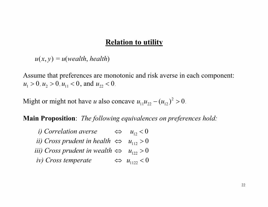
Relation to utility

( , )u x y = u(wealth, health)

Assume that preferences are monotonic and risk averse in each component:

1 0u > , 2 0u > , 11 0u < , and 22 0u < .

Might or might not have u also concave 2

11 22 12( ) 0u u u− > .

Main Proposition: The following equivalences on preferences hold:

i) Correlation averse ⇔ 12 0u <

ii) Cross prudent in health ⇔ 112 0u >

iii) Cross prudent in wealth ⇔ 122 0u >

iv) Cross temperate ⇔ 1122 0u <

23

Proof: We show (ii) here. Other cases are similar.

For a given ε% , define ( , ) ( , ) ( , )v x y u x y Eu x yε≡ − + % .

Analog to the utility premium, since y is fixed

Since 11 0u < , we have ( , ) 0v x y > .

Taking the derivative w.r.t. y, we obtain

2 2 2( , ) ( , ) ( , )v x y u x y Eu x yε≡ − + %

From Jensen’s inequality

2 ( , ) 0v x y < iff

2 ( , )u x y convex in x iff 112 ( , ) 0u x y > .

But 2 0v < iff ( , ) ( , ) ( , ) ( , )u x y Eu x y u x y c Eu x y cε ε− + < − − + −% %

Rearranging: 1 12 2[ ( , ) ( , )] [ ( , ) ( , )]u x y c Eu x y u x y Eu x y cε ε− + + > + + −% % . QED

24

EXAMPLES (with two-period reinterpretations of “lotteries”)

Precautionary saving against risky health status (let r = ρ = 0)

max ( ) ( , ) ( , )U s u x s y u x s y≡ − + +

FOC 1 1( , ) ( , ) 0u x s y u x s y− − + + = ⇒ s* = 0.

Now let health in period 2 be risky: (Note: No wealth consequences of ill health are assumed.)

max ( ) ( , ) ( , )U s u x s y Eu x s y δ≡ − + + + %

From FOC, s* > 0 if 1 1( , ) ( , )Eu x s y u x s yδ+ + > +% .

This follows whenever 1u is convex in y, i.e. 122 0u > . [Thus, cross prudence in wealth yields this precautionary savings demand.]

25

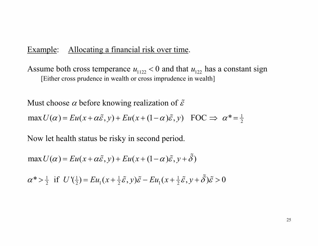
Example: Allocating a financial risk over time.

Assume both cross temperance 1122 0u < and that 122u has a constant sign [Either cross prudence in wealth or cross imprudence in wealth]

Must choose α before knowing realization of ε%

max ( ) ( , ) ( (1 ) , )U Eu x y Eu x yα αε α ε= + + + −% % FOC ⇒ 12

*α =

Now let health status be risky in second period.

max ( ) ( , ) ( (1 ) , )U Eu x y Eu x yα αε α ε δ= + + + − + %% %

12

*α > if 1 1 11 12 2 2

'( ) ( , ) ( , ) 0U Eu x y Eu x yε ε ε δ ε= + − + + >%% % % %

26

Holds if 11 2

( , ) ( , )H x y Eu x yε ε≡ + % % is concave in y, H22 < 0

Since 122sgn[ ]u is constant and 1122 0u < , we obtain,

0

1 122 122 1222 20( , ) ( , ) ( ) ( , ) ( )H x y u x y dF u x y dFε ε ε ε ε ε

+∞

−∞= + + +∫ ∫

0

122 1220

( , ) ( ) ( , ) ( ) 0u x y dF u x y dFε ε ε ε+∞

−∞< + =∫ ∫ .

122 0u > less negative + more positive

122 0u < more positive + less negative

Thus, the cross temperate individual will accept more than half of the ε% -risk in the first period.

27

CONCLUDING REMARKS

UP important part of risky-decision analysis

precautionary savings, 2nd-order effect in the small

Simple 50-50 lottery preferences is amenable to experimentation.

Necessary & sufficient conditions to sign cross derivatives.

Provide new examples of applications.

We make no normative claims about these signs. (Signing the cross derivatives has strong implications.)

E.g. Simple case of correlation aversion:

Viscusi & Evans (AER, 1990) provide empirical data to support 12 0u >

Evans & Viscusi (Re. Stat., 1991) find opposite result 12 0u < .