the equity premium implied by production -...

The Equity Premium Implied by Production

Urban J. Jermann∗

The Wharton School of the University of Pennsylvania and NBER

September 5, 2005

Abstract

We study the implications of producers’ first-order conditions for the link between invest-ment and aggregate asset prices. We provide a characterization of the determinants of theequity premium. Specifically, we present a closed form expression for the Sharpe ratio atsteady-state as a function of investment volatility and adjustment cost curvature only. Cali-brated to the U.S. postwar economy, the model can generate a sizeable equity premium, withreasonable volatility for market returns and risk free rates. The market’s Sharpe ratio and themarket price of risk are very volatile. Contrary to most models, our model generates a negativecorrelation between conditional means and standard deviations of excess returns.

In the twenty years since Mehra and Prescott’s paper on the equity premium puzzle many

studies have proposed and evaluated utility functions for their ability to explain the most salient

aggregate asset pricing facts. Several specifications have demonstrated their ability to improve con-

siderably over a basic time-separable constant relative risk aversion setup. Despite the progress

made, however, it seems that we have not yet reached the state where there would be a widely

accepted replacement for the standard time-separable utility specification. Contrary to the con-

sumption side, the production side of asset pricing has received considerably less attention. Fo-

cusing on the production side shifts the burden towards representing production technologies and

interpreting production data. While a number of asset pricing studies have considered nontrivial

production sectors, these have generally been studied jointly with some specific preference spec-

ification. Thus, the analysis could not escape the constraints imposed by the preference side. A

pure production asset pricing literature has emerged from the Q-theory of investment. However,

typically, these studies focus on the link between investment and realized stock returns, but not

on the equity premium.1

∗I am grateful for the comments received from seminar participants at Wharton, UBC, BI School, the Board

of Governors, the Federal Reserve Bank of Philadelphia, NYU, the SED meeting and from Andy Abel, Harjoat

Bhamra, Joao Gomes and Stavros Panageas, and for research assistance by Jianfeng Yu. The most recent version

of this paper can be found at http://finance.wharton.upenn.edu/~jermann/research.html1An incomplete list of contributions include: for successful utility functions, Abel (1990), Campbell and Cochrane

1

USC FBE DEPT. MACROECONOMICS &INTERNATIONAL FINANCE WORKSHOPpresented by Urban JermannFRIDAY, March 24, 20063:30pm - 5:00 pm, Room: HOH-601K

In this paper we are interested in studying the macroeconomic determinants of asset prices

given by a multi-input aggregate production technology. We focus exclusively on the producers’

first-order conditions that link production variables and state-prices, with sectoral investment play-

ing the key role. We are interested in two sets of questions. First: what properties of investment

and production technologies are important for the first and second moments of risk free rates and

aggregate equity returns? Second: does a model plausibly calibrated to the U.S. economy have

the ability to replicate first and second moments of risk free rates and aggregate equity returns?

The work most closely related to ours is Cochrane’s work on production-based asset pricing

(1988, 1991). Some of the features that differentiate our work are that we focus explicitly on the

equity premium, we use more general functional forms for adjustment cost, and we base our empir-

ical evaluation on the two main sectoral aggregates of U.S. capital investment, namely equipment

& software as well as structures. Cochrane (1993) derives a set of asset pricing implications of a

production function where the productivity level can be selected in a state-contingent way.

We consider the problem of a representative producer that selects multiple fixed input factors.

In order to be able to recover a state-price process, our setup needs to have two related properties.

First, markets need to be complete and the producer has to face a full set of state-prices. Second,

there needs to be as many predetermined state variables (fixed production factors) as there are

states of nature. This assumption of “complete technologies” is necessary in order to be able

to recover the full set of state-contingent prices from the production side. In most studies with

nontrivial production sectors this property is not satisfied; of course, in a general equilibrium

environment it doesn’t usually play such an important role.

We calibrate our model to a two-sector representation. We use U.S. data on investment for

equipment and software, as well as for structures. This sectoral representation is convenient

because these two sectors have natural asymmetries. Indeed, we use the plausible assumption that

the capital stock for structures is more difficult to adjust than for equipment and software. As

becomes clear below, asymmetries across sectors are crucial for asset prices.

We characterize sectoral asymmetries that ensure that state-prices are positive and that gen-

erate a positive equity premium. Specifically, we present a closed form expression for the Sharpe

ratio at steady-state as a function of investment volatility and adjustment cost curvature only.

We also show that there is an upper bound to the Sharpe ratio more generally in two-state en-

(1999), Constantinides (1990); for models with nontrivial production sectors Jermann (1998) and Rouwenhorst

(1995); for production asset pricing studies, Cochrane (1988, 1991), Li, Vassalou and Xing (2003), and Gomes,

Yaron and Zhang (2002). Other examples of related asset pricing studies with rich production structures are Berk,

Green and Naik (1999), Carlson, Fisher and Giammarino (2003), Hugonnier, Morellec and Sundaresan (2005), and

Tuzel (2004).

2

vironments. Our key quantitative findings are the following. For unconditional moments, we can

plausibly generate an equity premium of several percentage points with risk free rates having a

reasonable mean and volatility. For conditional moments, the expected excess equity return is

quite volatile, usually more volatile than the risk free rate. Also concerning excess returns, the

correlation between conditional means and volatilities is negative.

The paper is organized as follows. In section 1, we present the model and in section 2 some asset

pricing elements. Section 3 introduces functional forms. In section 4 we characterize theoretical

links between asset prices and investment. Section 5 contains our calibration and section 6 the

quantitative analysis.

1 Model

The model represents the producer’s choice of capital inputs for a given state price process.

Key ingredients are capital adjustment cost and stochastic productivity.

Assume an environment where uncertainty is modelled as the realization of s, one out of a

finite set S = (s1, s2, ...sN), with st the current period realization and st ≡ (s0, s1, ...st) the historyup to and including t. Probabilities of st are denoted by π

¡st¢. Assume an aggregate production

function

Y¡st¢= F

³©Kj¡st−1

¢ªj∈J , s

t, N¡st¢´,

st introduces possible stochastic technology in the production of the final good, Kj is the j-th

capital stock, N labor. Capital accumulation for capital good of type j is represented by

Kj¡st¢= Kj

¡st−1

¢(1− δj) + Zj

¡st¢Ij¡st¢,

where δj is the depreciation rate and Zj¡st¢the (stochastic) technology for producing capital

goods. We assume Zj¡st¢= Zj

¡st−1

¢ ·λZj (st), with λZj (st) following a N -state Markov process.The total cost of investment in capital good of type j is given by

Hj¡Kj¡st−1

¢, Ij¡st¢, Zj

¡st¢¢.

This specification will be further specialized below.

The representative firm solves the following problem taking as given state prices P¡st¢

max{I,K0,N}

∞Xt=0

Xst

P¡st¢⎡⎣F ³©Kj ¡st−1¢ªj∈J , st, N ¡st¢´− w ¡st¢N ¡st¢−X

j

Hj¡Kj¡st−1

¢, Ij¡st¢, Zj

¡st¢¢⎤⎦

s.t. :£P¡st¢qj¡st¢¤: Kj

¡st−1

¢(1− δj) + Zj

¡st¢Ij¡st¢−Kj ¡st¢ ≥ 0, ∀st, j

3

with s0 and Kj (s−1) given and P (s0) = 1, without loss of generality. The scaling of the

multipliers is chosen so that we get intuitive labels. Indeed, q represents the marginal value of

one unit of installed capital in terms of the numeraire of the same period. In equilibrium, it is

also the cost of installing one unit of capital including adjustment cost. Note, for U.S. data on

equipment and software, Z has a strong positive growth trend. Then, q in this sector will be

trending down—reflecting the fact that equipment and software become cheaper over time. Also

note that q is not the ratio of the market value over the book value of capital, that is Tobin’s Q,

but qZ is. The book value (or replacement cost) of the capital stock is K/Z, where K is number

of units of the capital good and 1/Z = pI the price of a unit of capital in terms of the final good.

First-order conditions are summarized by

0 = −Hj,2¡Kj¡st−1

¢, Ij¡st¢, Zj

¡st¢¢+ Zj

¡st¢qj¡st¢,

qj¡st¢=Xst+1

P¡st, st+1

¢P (st)

·nFKj

³©Ki¡st¢ªi∈J , s

t, st+1, N¡st, st+1

¢´−Hj,1 ¡Kj ¡st¢ , Ij ¡st, st+1¢ , Zj ¡st, st+1¢¢+ (1− δj) qj¡st, st+1

¢oand for N ,

FN¡©Kj¡st−1

¢ª, st, N

¡st¢¢− w ¡st¢ = 0

so that substituting out shadow prices we have

Xst+1

P¡st+1|st

¢⎡⎣ FKj

¡©Kj¡st¢ª, st, st+1, N

¡st, st+1

¢¢−Hj,1

¡Kj¡st¢, Ij¡st, st+1

¢, Zj

¡st, st+1

¢¢+ (1− δj)

Hj,2(Kj(st),Ij(st,st+1),Zj(st,st+1))Zj(st,st+1)

⎤⎦·"

Zj¡st¢

Hj,2 (Kj (st−1) , Ij (st) , Zj (st))

#= 1,

for each j, where the notation P¡st+1|st

¢shows the price of the numeraire in st+1 conditional

on st and in units of the numeraire at st. From this condition we define the investment return

RIj¡st, st+1

¢implicitly through

Pst+1

P¡st+1|st

¢RIj¡st, st+1

¢= 1. RIj

¡st, st+1

¢is the return we

get in st+1 from adding one (marginal) unit of capital of type j in state st. The first-order condition

shows that in equilibrium adding one marginal unit of a given type of capital produces a change

in the profit plan that is worth one unit.2

We will specialize the model to have 2 capital inputs and 2 states of nature in each period. In

addition to complete markets, that is the producers ability to sell contingent output for each state

of nature, we also need to satisfy the requirement of “complete technologies”, that is the ability to

move resources independently between all states of nature. This complete technology requirement

is needed if we want to be able to recover all state prices from the producers first-order conditions.2Based on the details given below, strict concavity will be assumed, so that first-order and transversality condi-

tions (given below) are sufficient for a maximum.

4

2 From investment returns to state prices and asset returns

Representing the first-order conditions in matrix form we have⎡⎣ RI1 ¡st, s1¢ RI1¡st, s2

¢RI2¡st, s1

¢RI2¡st, s2

¢⎤⎦⎡⎣ P ¡s1|st¢

P¡s2|st

¢⎤⎦ = 1, or compactly: RI ¡st¢ · p ¡st¢ = 1 (2.1)

so that the state price vector is obtained from matrix inversion

p¡st¢=¡RI¡st¢¢−1

1.

Clearly, it isn’t necessarily the case that this matrix inversion is feasible nor that state prices are

necessarily positive for any chosen set of returns. As further discussed below, the requirement for

positive state prices will constrain our empirical implementation.

In this environment, the risk free return is given by:

1/Rf¡st¢= 1p

¡st¢= P

¡s1|st

¢+ P

¡s2|st

¢.

It is easy to check the matrix algebra to see that if for one of the investment returns the realized

return is not state-contingent RIj¡st, st+1

¢= RIj

¡st¢, then, as is implied by no-arbitrage, it equals

the risk free rate, RIj¡st¢= Rf

¡st¢.

Now, consider aggregate equity returns

R¡st, st+1

¢=D¡st, st+1

¢+ V

¡st, st+1

¢V (st)

,

whereD¡st, st+1

¢= F

¡©Kj¡st−1

¢ª, st, N

¡st¢¢−w ¡st¢N ¡st¢−Pj Hj

¡Kj¡st−1

¢, Ij¡st¢, Zj

¡st¢¢

represents the dividends paid by the firm and V¡st, st+1

¢the ex-dividend value of the firm. As-

suming constant returns to scale in F (.) andHj (.), Hayashi’s (1982) result applies, and this return

will be equal to a weighted average of the investment returns:

R¡st, st+1

¢=Xj

qj¡st¢Kj¡st¢P

i qi (st)Ki (st)

·RIj¡st, st+1

¢. (2.2)

The market price of risk, aka the highest Sharpe ratio, also has a simple expression. Let us,

introduce the stochastic discount factor m¡st+1|st

¢by dividing and multiplying through by the

probabilities π¡st+1|st

¢, so that

P¡st+1|st

¢=

ÃP¡st+1|st

¢π (st+1|st)

!π¡st+1|st

¢= m

¡st+1|st

¢π¡st+1|st

¢.

Then, ruling out arbitrage implies Et¡m¡st+1|st

¢Re¡st, st+1

¢¢= 0, for ∀Re ¡st, st+1¢ defined as

excess returns. It is then easy to see that

maxE£Re¡st, st+1

¢ |st¤Std [Re (st, st+1) |st] =

vuuutPst+1

P (st+1|st)2 /π (st+1|st)hPst+1

P (st+1|st)i2 − 1.

5

3 Functional Forms

In this section, we present the functional forms and the simulation strategies.

A. The investment cost function

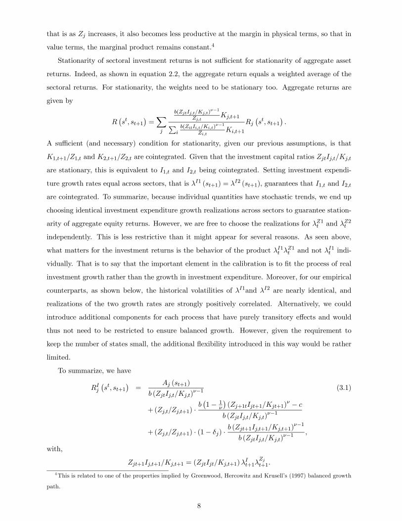
The investment cost function is chosen so as to allow for the ability to have different adjustment

cost curvatures across sectors and for balanced growth. We will use the following specification

H (K, I, Z) = H (K/Z, I) = H (1, ZI/K) · (K/Z)

so that it is homogenous of degree 1 in I and K/Z to guarantee balanced growth.3

The functional form is assumed to be

H (1, ZI/K) · (K/Z) =½b

ν(ZI/K)ν + c

¾(K/Z) ,

with b, c > 0, ν > 1 and ZI/K ≥ 0.As can easily be seen, this function is (1) convex in I for ν > 1. (2) adjustment cost and the

direct cost for additional capital goods are separable, trivially so because H (1, ZI/K) · (K/Z) =[H (1, ZI/K)− ZI/K + ZI/K] · (K/Z) = [H (1, ZI/K)− ZI/K] · (K/Z) + I ≡ C (1, ZI/K) ·(K/Z) + I. We impose restrictions on the parameters of H (.) so that C (1, ZI/K) ≥ 0, that is,the pure adjustment cost is nonnegative.

The different parameters have roughly the following functions. ν determines the cost of choos-

ing volatile investment plans. For a given investment process, it determines the volatility of the

market price of capital. The parameters b and c are used to obtain target values for qZ (marginal

cost) and for the total cost.

With this specification, we have the marginal cost given as

HI (K, I, Z) = H2 (1, ZI/K) = b (ZI/K)ν−1 ,

and we can easily check convexity with respect to investment

HII (K, I, Z) = b (ν − 1) (ZI/K)ν−2 (Z/K) > 0 for b > 0 and ν > 1.

The case of no-adjustment cost is given by setting ν = b = 1, c = 0, so that

H (1, ZI/K) · (K/Z) = I.3Given the capital accumulation equation, and as we further discuss below, IZ and K are cointegrated, and so

are I and K/Z.

6

From the first-order condition we obtain a relationship between the investment rate and the

marginal cost of capital

qZ = HI (K, I, Z) = b (ZI/K)ν−1 .

Normalizing Z to 1,the elasticity (quantity elasticity of a price) of qwith respect to I/K is

∂q

∂ (I/K)

I/K

q= ν − 1.

B. Simulation strategy and stationarity of returns

For our quantitative analysis, we will assume that we know the optimal investment process.

We then derive the implied investment returns and state-prices. We will assume that investment

follows a two-state Markov process. For our simulations, we want returns to be stationary. This

imposes some restrictions on technologies and the assumed optimal investment process. In this

section we discuss these issues in detail.

Consider the investment return for capital stock j given our functional forms

RIj¡st, st+1

¢= Zjt ·

FKj


¡st, st+1

¢¢b (ZjtIj,t/Kj,t)

ν−1 + (Zj,t/Zj,t+1) ·b¡1− 1

ν

¢(Zj+1tIjt+1/Kjt+1)

ν − cb (ZjtIj,t/Kj,t)

ν−1

+(Zj,t/Zj,t+1) · (1− δj) · b (Zjt+1Ij,t+1/Kj,t+1)ν−1

b (ZjtIj,t/Kj,t)ν−1 ,

where we have used a more compact notation for state-dependence. The first term represents

the marginal product, the second the adjustment cost reduction next period (growth option) and

the third, the leftover capital. A sufficient set of conditions for RIj¡st, st+1

¢to be stationary is

that each of the 3 different composite variables is stationary. Let us consider each of these terms

separately.

First, Zj,t+1/Zj,t, as seen above, is stationary by assumption. Second, given the specification of

the productivity growth rates as finite elements Markov chains, and assuming that sectoral invest-

ment growth rates also follow finite element Markov chains, that is, Ij¡st, st+1

¢= Ij

¡st¢λIj (st+1),

it can easily be shown that for appropriate starting points, ZjtIj,t/Kj,t is bounded. Third, we will

make the assumption that the production function is such that

ZjtFKj


¡st, st+1

¢¢ ≡ Aj (st+1) .This guarantees stationarity and allows us to focus our analysis on investment dynamics. One

implication of this assumption is that to the extent that capital gets cheaper to produce over time,

7

that is as Zj increases, it also becomes less productive at the margin in physical terms, so that in

value terms, the marginal product remains constant.4

Stationarity of sectoral investment returns is not sufficient for stationarity of aggregate asset

returns. Indeed, as shown in equation 2.2, the aggregate return equals a weighted average of the

sectoral returns. For stationarity, the weights need to be stationary too. Aggregate returns are

given by

R¡st, st+1

¢=Xj

b(ZjtIj,t/Kj,t)ν−1

Zj,tKj,t+1P

ib(ZitIi,t/Ki,t)

ν−1

Zi,tKi,t+1

Rj¡st, st+1

¢.

A sufficient (and necessary) condition for stationarity, given our previous assumptions, is that

K1,t+1/Z1,t and K2,t+1/Z2,t are cointegrated. Given that the investment capital ratios ZjtIj,t/Kj,t

are stationary, this is equivalent to I1,t and I2,t being cointegrated. Setting investment expendi-

ture growth rates equal across sectors, that is λI1 (st+1) = λI2 (st+1), guarantees that I1,t and I2,t

are cointegrated. To summarize, because individual quantities have stochastic trends, we end up

choosing identical investment expenditure growth realizations across sectors to guarantee station-

arity of aggregate equity returns. However, we are free to choose the realizations for λZ1t and λZ2t

independently. This is less restrictive than it might appear for several reasons. As seen above,

what matters for the investment returns is the behavior of the product λI1t λZ1t and not λI1t indi-

vidually. That is to say that the important element in the calibration is to fit the process of real

investment growth rather than the growth in investment expenditure. Moreover, for our empirical

counterparts, as shown below, the historical volatilities of λI1and λI2 are nearly identical, and

realizations of the two growth rates are strongly positively correlated. Alternatively, we could

introduce additional components for each process that have purely transitory effects and would

thus not need to be restricted to ensure balanced growth. However, given the requirement to

keep the number of states small, the additional flexibility introduced in this way would be rather

limited.

To summarize, we have

RIj¡st, st+1

¢=

Aj (st+1)

b (ZjtIj,t/Kj,t)ν−1 (3.1)

+(Zj,t/Zj,t+1) ·b¡1− 1

ν

¢(Zj+1tIjt+1/Kjt+1)

ν − cb (ZjtIj,t/Kj,t)

ν−1

+(Zj,t/Zj,t+1) · (1− δj) · b (Zjt+1Ij,t+1/Kj,t+1)ν−1

b (ZjtIj,t/Kj,t)ν−1 ,

with,

Zjt+1Ij,t+1/Kj,t+1 = (ZjtIjt/Kj,t+1)λIt+1λ

Zjt+1.

4This is related to one of the properties implied by Greenwood, Hercowitz and Krusell’s (1997) balanced growth

path.

8

Thus, realized returns are given as functions of the following

RIj¡st, st+1

¢= RIj

¡Zj¡st¢Ij¡st¢/Kj

¡st−1

¢;λI (st+1) ,λ

Zj (st+1) , Aj (st+1)¢for j = 1, 2.

For our simulations, we will generate realizations of all quantities of interest based on a probability

matrix describing the law of motion for the exogenous state st+1. The law of motion for the rest

of the variables follows

Ij¡st, st+1

¢= Ij

¡st¢λI (st+1) for j = 1, 2

Zj¡st, st+1

¢= Zj

¡st¢λZj (st+1) for j = 1, 2

Kj¡st¢= Kj

¡st−1

¢(1− δj) + Zj

¡st¢Ij¡st¢for j = 1, 2.

Seven variables are a sufficient statistic for the current state of the economy st, namely

st,K1¡st−1

¢,K2

¡st−1

¢, I1¡st¢, I2¡st¢, Z1

¡st¢, Z2

¡st¢. Clearly Kj

¡st¢matters too, but it is

a function of the state variables. The probability distribution of the shocks is summarized

by st, the realization of the return does not depend on st. As initial conditions, we will set

K2¡s−1¢= Z1

¡s0¢= Z2

¡s0¢= 1, and K1

¡s−1¢is set equal to the historical average of the

ratio of the value of capital in this sector relative to the other sector. Initial investment levels are

assumed at their implied steady state values.

4 Theoretical analysis

In this section we present a series of theoretical results that help us understand key model

mechanisms. First, we show how the equity premium is determined from investment returns, and

how investment returns are determined from investment growth. Second, we discuss in detail

what constitutes an admissible investment process for a given technology specification. Third,

we present the conditions under which we can recover state prices in a model without technology

shocks. A key finding of this section is that sectoral differences in the adjustment cost parameters

νj are crucial for allowing us to recover admissible state prices from investment. We present a

simple expression for the Sharpe ratio that depends only on the investment cost curvature and

the investment volatility. This expression shows that there is a minimum amount of curvature

required to have a positive equity premium. We also derive an upper bound for the Sharpe ratio,

and discuss to what extent this can explain some of our quantitative findings. Another key finding

is that in a model without technology shocks and where interest rates are constant, investment

returns have to be constant. Thus, in such an environment, it is not possible to recover state

prices from producers first-order conditions.

9

A. What determines the equity premium?

We consider here the relationship between investment and asset prices by focusing on the

requirements for a positive equity premium. For this issue, a continuous-time representation is

more intuitive than our discrete-time model used sofar. There are two main findings in this

section. First, we show that in order to have a positive equity premium, the investment return

with the higher expected return needs to be the more volatile. Second, we show that under some

conditions, asymmetries in the investment cost curvature ν can generate this property, and we

present a simple expression for the Sharpe ratio.

In parallel to our two-state representation in discrete time, assume we have a one-dimensional

Brownian motion. Investment returns are given by

dRjRj

= µj (.) dt+ σj (.) dz, for j = 1, 2, (4.1)

and assume that the state-price process also follows such a process

dΛ

Λ= −rf (.) dt+ σ (.) dz. (4.2)

We will assume that the two returns are positively (perfectly) correlated so that sign (σ1) =

sign (σ2). We allow for the drift and diffusion coefficients to change with the state of the economy.

For compactness, from now own, our notation will not explicitly acknowledge this.

We want to derive the drift and diffusion terms of the state-price process, −rf and σ, from

the given return processes, that is from the four values µj and σj for j = 1, 2. Remember, in this

environment, the absence of arbitrage implies that

0 = Et

µdΛtΛt

¶+Et

µdRjtRjt

¶+Et

µdΛtΛt

dRjtRjt

¶, (4.3)

so that we have

0 = −rfdt+ µidt+ σiσdt,

and thus 2 equations and 2 unknowns. The solution of this system is

rf =σ2µ1 − σ1µ2σ2 − σ1

−σ =µ2 − µ1σ2 − σ1

.

In order to be able to recover the state price process from the two returns, we need σ2−σ1 6= 0.That is, the volatility terms have to be different across sectors; and, implicitly, if we assume

continuous loadings of the return processes, their ordering is not allowed to change. This is an

invertibility requirement similar to the one for the discrete time case. Compared to the discrete

10

time case, there is no issue of possibly negative state prices as we discuss below. Indeed, a process

such as 4.2 cannot become negative if initially positive.

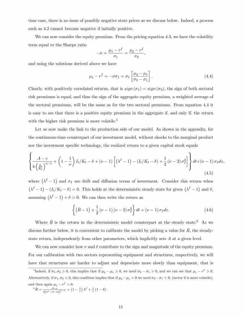
We can now consider the equity premium. From the pricing equation 4.3, we have the volatility

term equal to the Sharpe ratio

−σ = µ1 − rfσ1

=µ2 − rf

σ2,

and using the solutions derived above we have

µ1 − rf = −σσ1 = σ1

∙µ2 − µ1σ2 − σ1

¸. (4.4)

Clearly, with positively correlated returns, that is sign (σ1) = sign (σ2), the sign of both sectoral

risk premiums is equal, and thus the sign of the aggregate equity premium, a weighted average of

the sectoral premiums, will be the same as for the two sectoral premiums. From equation 4.4 it

is easy to see that there is a positive equity premium in the aggregate if, and only if, the return

with the higher risk premium is more volatile.5

Let us now make the link to the production side of our model. As shown in the appendix, for

the continuous-time counterpart of our investment model, without shocks to the marginal product

nor the investment specific technology, the realized return to a given capital stock equals⎧⎪⎨⎪⎩ A− cb³ItKt

´ν−1 +µ1− 1ν¶It/Kt − δ + (ν − 1)

∙¡λI − 1¢− (It/Kt − δ) +

1

2(ν − 2)σ2I

¸⎫⎪⎬⎪⎭ dt+(ν − 1)σIdz,(4.5)

where¡λI − 1¢ and σI are drift and diffusion terms of investment. Consider this return when¡

λI − 1¢− (It/Kt − δ) = 0. This holds at the deterministic steady state for given¡λI − 1¢ and δ,

assuming¡λI − 1¢+ δ > 0. We can then write the return as½¡

R̄− 1¢+ 12(ν − 1) (ν − 2)σ2I

¾dt+ (ν − 1)σIdz. (4.6)

Where R̄ is the return in the deterministic model counterpart at the steady state.6 As we

discuss further below, it is convenient to calibrate the model by picking a value for R̄, the steady-

state return, independently from other parameters, which implicitly sets A at a given level.

We can now consider how ν and δ contribute to the sign and magnitude of the equity premium.

For our calibration with two sectors representing equipment and structures, respectively, we will

have that structures are harder to adjust and depreciate more slowly than equipment, that is

5 Indeed, if σ1,σ2 > 0, this implies that if µ2 − µ1 > 0, we need σ2 − σ1 > 0, and we can see that µ1 − rf > 0.Alternatively, if σ1,σ2 < 0, this condition implies that if µ2−µ1 > 0 we need σ2−σ1 < 0, (sector 2 is more volatile),

and then again µ1 − rf > 0.6 R̄ = A−c

b(λI−(1−δ))v−1+¡1− 1

v

¢λI + 1

v(1− δ) .

11

νS > νE, and δS < δE. We label equipment as sector 1, and thus ν2 > ν1. As is clear from

equation (4.6), for a given R̄, there is no separate role for depreciation rates at steady state. We

now show under what conditions we have a positive equity premium at steady state.

Because (ν − 1) multiplies σIdz, with our sectoral normalization, the volatility term of sector

2 is larger, that is σ2 > σ1, assuming equal investment volatility σI across sectors. To see whether

this asymmetry can generate a positive equity premium, we need to check the effect of ν on the

drift component. It is easy to see that

∂ (ν − 1) (ν − 2)∂ν

= 2

µν − 3

2

¶→ if ν >

3

2then

∂ (ν − 1) (ν − 2)∂ν

> 0.

That is, starting from a common curvature parameter ν > 32 , and increasing curvature in one

sector, the sector with the higher curvature will have a higher drift, everything else equal. Thus,

if ν > 1.5, and if there are no sectoral asymmetries except the difference in ν, we have σ2 > σ1and

µ2 > µ1, that is, as shown in equation 4.4 above, the equity premium is positive.

We can directly compute the Sharpe ratio at steady state, assuming R̄j = R̄ and σIj = σI , as

µj − rfσj

|ss = ν1 + ν2 − 32

σI . (4.7)

Because, σj and σI have the same sign (given νj > 1), a necessary and sufficient condition for a

positive equity premium is that ν1+ ν2 > 3. Clearly, the equity premium is then increasing in the

sum of the curvature parameters.

In our calibration we set R̄2 and R̄1 independently from other parameters as a way of implicitly

selecting values of Aj . Given the limited amount of precise direct information about Aj , we choose

this approach. Alternatively, we could take all coefficients determining R̄ as given, and consider

the partial derivatives with respect to ν and δ. A few steps of algebra show that under the standard

assumptions that ν > 1, λ− 1− δ > 0, and (A− c) /b (λ− (1− δ))ν−1 > 0, ∂R̄∂ν > 0, and

∂R̄∂δ < 0.

Therefore, given our assumed sectoral asymmetries, both would contribute to µ2 > µ1, and with

σ2 > σ1, this would contribute positively to the equity premium.

We can also compute the instaneous interest rate at steady state, assuming R̄j = R̄ and

σIj = σI , as

rf |ss =¡R̄− 1¢− (v1 − 1) (v2 − 1) σ2I

2.

This expression shows how investment uncertainty contributes to a lower steady state interest rate

by an extent that is determined by the amount of the adjustment cost curvature. This parallels

the precautionary saving effect on interest rates in standard consumption based models.

12

B. What is an admissible investment process?

In this section we consider the requirements for an investment process to be admissible, in the

sense that it represents a solution to the firm’s problem for the implied state-price process, and

that this price process is itself well behaved. The two key requirements are that the derived state

prices have to be positive and that the implied firm value has to be finite. While a large set of

investment processes are admissible, these requirements nevertheless impose constraints on our

simulations. For this reason, this section also provides the motivations for some of the choices we

make in our empirical analysis.

(i) Positive state prices The first key requirement is that state prices have to be positive. It is

easy to see from equation 2.1 that the relative state prices in the two-state case are given by

P¡st, s1

¢P (st, s2)

=RI2¡st, s2

¢−RI1 ¡st, s2¢RI1 (s

t, s1)−RI2 (st, s1). (4.8)

As can easily be seen, for nonnegative investment returns, that is R > 0, state prices are positive

if and only if numerator and denominator have the same sign. Economically, this requirement

implies that each capital stock has to do (absolutely) better in one state. Indeed, if one type of

investment were to generate a higher return in both states, then resources would be moved into

this type of capital from the other, meaning that this is not an equilibrium outcome.7

To see what properties are needed to satisfy this requirement, consider now a second order

Taylor-series approximation of the investment return in equation (4.10, which is the discrete time

counterpart of the continuous-time return equation 4.6 discussed above. The second-order Taylor

approximation of the investment return is at the steady-state investment capital level around the

mean of investment growth. To focus on the quantitatively important channel, we again assume

that only investment expenditure growth is allowed to vary, but not the marginal product nor

the investment specific technology. Under these assumptions, we can rewrite equation 3.1 for the

investment return as

RIt,t+1¡st, sj

¢=

A− cb³

It(st)Kt(st−1)

´ν−1+⎧⎪⎨⎪⎩(1− δ) +

µ1− 1

ν

¶⎡⎢⎣ It(st)Kt(st−1)

It(st)Kt(st−1) + (1− δ)

⎤⎥⎦λ (st+1)⎫⎪⎬⎪⎭⎛⎝ 1

It(st)Kt(st−1) + (1− δ)

λ (st+1)

⎞⎠ν−1

.

(4.9)

This expression makes it clear how in this case realized returns are a function of the realization of

investment growth rate λ (st+1), while the only relevant state variable is the current investment-

capital ratio It¡st¢/Kt

¡st−1

¢. A second-order Taylor approximation is obtained by assuming that

the investment-capital ratio is at its steady state It¡st¢/Kt

¡st−1

¢= λ̄− 1 + δ,

7A related requirement is that the matrix R has to be invertible for us to be able to recover the state prices.

13

RIt,t+1 = R̄+ (ν − 1)∆λ0 +B

2

¡∆λ0

¢2+ o

³¡∆λ0

¢2´ (4.10)

where ∆λ0 = λ0 − E ¡λ0¢. The only difference compared to the continuous-time equation is thesecond-order term. Here it equals

B =ν − 1λ

½ν − 1− 1− δ

λ

¾.8

Assuming IID investment shocks, the size of the up and down deviations from the mean in a

two-state setting are identical, that is, we have

∆λj (s2) = −∆λj (s1) ≡ ∆λj , for each j ∈ (1, 2) .

Moreover, assuming equal investment growth volatility in the two sectors (a reasonable assumption

as we discuss later) and positive correlation, we have

∆λ1 = ∆λ2 = ∆λ.

Introduce this approximation into the ratio determining relative state prices,

P (., s1)

P (., s2)=[ν2 − ν1]∆λ+

h¡R̄2 − R̄1

¢+ 1

2 (B2 −B1)¡∆λ¢2i

+ o³¡∆λ¢2´

[ν2 − ν1]∆λ−h¡R̄2 − R̄1

¢+ 1

2 (B2 −B1)¡∆λ¢2i

+ o³¡∆λ¢2´ (4.11)

As shown by equation 4.11, in order to have positive prices, the first term in the fraction needs

to be far away from zero, that is [ν2 − ν1]∆λ >> 0 or << 0. This terms needs to be sufficiently far

away from 0 so that the remaining terms in the fraction cannot overturn the sign of the numerator

and the denominator. Moreover, this first-order term should not be too sensitive to the state of

the economy so as to ensure that this property is satisfied everywhere. Thus, clearly, asymmetry

in ν is needed to generate positive state prices, while the level of δ plays no role.

One issue we face in our numerical experiments is that the investment capital ratio can reach

very low levels. In this case, the coefficients of a second-order approximation around the current

investment-capital ratio can differ substantially from their steady state values. Specifically, as can

be seen from equation (4.9), investment returns can get infinitely large as It¡st¢/Kt

¡st−1

¢gets

close to 0. Indeed, the first term (A− c) /bµ

It(st)Kt(st−1)

¶ν−1can get infinitely large. Under these

conditions, the requirement for positive state prices may be hard to satisfy for all possible paths.

What makes this condition hard to satisfy is that it has to hold with probability one. In our

simulations we choose to make the marginal product terms, A, state contingent and to select its

value in the low growth state specifically so that state prices are positive for the lowest possible8With (1− δ) = λ = 1, we would have B = (v − 1) (v − 2), which is the term in the continuous time counterpart.

Note, we have also made the assumption here that E (λ0) = λ̄.

14

It¡st¢/Kt

¡st−1

¢. As we show below, shocks to A have only second order effects on asset price

implications in general. This is because the level of A is so small relative to the other terms in the

return equation 4.9.

(i).1 Upper bound for Sharpe ratio The requirement for nonnegative state prices has an impli-

cation for two-state environments in general, that we present here. Namely, if the two states are

equally likely, the Sharpe ratio is bounded by 1. Because we never deviate much from this case in

our simulations, we typically are bound by this constraint. Moreover, because the requirement of

positive state prices has to hold with probability one, the constraints on the technology and the

investment process end up reducing average Sharpe ratios to levels substantially lower than 1.

In a two-state environment, no arbitrage requires that for the excess return on the market

RM (s)−Rf ,P (s1)

³RM (s1)−Rf

´+ P (s2)

³RM (s2)−Rf

´= 0.

This implies that, in line with our equation (4.8), the ratio of the state prices is given by

P (s1)

P (s2)=

¡RM (s2)−Rf

¢− (RM (s1)−Rf ) =

£RM (s2)−ERM

¤+£ERM −Rf¤

− [RM (s1)−ERM ]− [ERM −Rf ] .

It is easy to see that if both states are equally likely then we have£RM (s2)−ERM

¤= − £RM (s1)−ERM¤ =

Std¡RM

¢, so that

P (s1)

P (s2)=Std

¡RM

¢+£ERM −Rf¤

Std (RM)− [ERM −Rf ] .9

Because of the requirement of positive state prices, the denominator has to be positive, and

therefore the Sharpe ratio, ERM−Rf

Std(RM ), is bounded,

Std¡RM

¢>

hERM −Rf

i1 >

ERM −RfStd (RM)

.

Clearly, this result applies to all models without arbitrage in a two-state environment. For instance,

it applies to the classic model used by Mehra and Prescott (1985). Based on the history of sectoral

investment growth we consider in this study, a reasonable calibration cannot deviate much from

the case where up and down movements are equally likely. Thus, the result derived here is

relevant. Because the requirement of positive state prices has to hold with probability one, the

constraints on the technology and the investment process end up reducing average Sharpe ratios

in our simulations to a level substantially below 1. The non-IID case we consider, with first-order

9We have here implicitly normalized the environment so that RM (s2) > RM (s1). This is without loss of

generality.

15

serial correlation of 0.2, does not substantially affect quantitative findings as shown later in the

paper.10

(ii) Other requirements The second key requirement is that the value of the firm implied by

an investment process and a state price process has to be finite. If not, the equivalence between

investment returns and returns to the firm breaks down. A related condition that guarantees

optimality of the path satisfying the first-order condition is the transversality condition

limt→∞

Xst

P¡st¢

P (s0)

©A¡st¢+HI

¡st¢(1− δ)−HK

¡st¢ªKt¡st−1

¢= 0.

We check both conditions in our simulations. We also make sure that gross investment returns

are nonnegative, R ≥ 0. This limited liability requirement is not necessarily needed. On the otherhand, it doesn’t impact any quantitative conclusions.

(iii) Models with no technology shocks: Interest rates cannot be constant We consider here the

benchmark environment where the only source of uncertainty that firms face are stochastic state

prices. That is to say, there are no shocks to the production technology. We have one result: even

without technology shocks, investment returns can be optimally state-contingent as long as interest

rates are not constant. In an environment where interest rates are constant forever, investment

returns are constant too. Thus, with constant interest rates it is not possible to recover the state

price process from producers’ first-order conditions. The basic economic idea in this section is

that if a firm is subject to convex capital adjustment costs, it will not find it optimal to choose a

volatile investment plan unless forced by changing prospects in future valuations.

Consider the discrete-time model with no technology shocks. Assuming a general two-state

environment where state-prices do not necessarily have a Markov representation. The firm’s

problem is given by

max{I(st),K(st+1)}

T−1Xt=0

Xst

∙AKt (st−1)−

½b

ν

¡I¡st¢/Kt

¡st−1

¢¢ν+ c

¾Kt¡st−1

¢¸×⎛⎝t−1Yj=0

P¡sj+1|sj

¢⎞⎠+XsT

ΨKT¡sT−1

¢⎛⎝T−1Yj=1

P¡sj+1|sj

¢⎞⎠ ,subject to

0 = (1− δ)Kt¡st−1

¢+ I

¡st¢−Kt+1 ¡st¢ ,

10For the case with unequal probabilities, through a similar argument, we can obtain a boundµ1− π

π

¶0.5>

£ERM −Rf ¤std (RM )

,

where π is the probability of the state with the low return realization. Thus, with postively skewed returns the

bound is tighter, with negatively skewed returns it is looser.

16

with K (s0) given, P¡s0|s0

¢= 1, and Ψ > 0 a parameter; assuming that st ∈ (s1, s2).

The solution of this problem for T →∞ is equivalent to the solution of the general version of

our problem with enough regularity so that firm value is finite. However, it is easy to see in this

model why interest rate volatility is needed. Indeed, from T − 1 to T , without technology shocks,the return to capital equals the risk free rate. For the second-to-last return-period, that is, from

T − 2 to T − 1, it can be checked that the return is given by

RT−2,T−1¡sT−2, sj

¢=

α

µΨ

RfT−1,T (sT−2,sj)

¶α

µΨ

RfT−1,T (sT−2,s1)

¶P (s1|sT−2) + α

µΨ

RfT−1,T (sT−2,s2)

¶P (s2|sT−2)

, for j = 1, 2.

with α (x) = (A− c)+(1− δ)x+¡1− 1

ν

¢ ¡1b

¢ 1ν−1 x

νν−1 . Clearly, if the interest rateRfT−1,T

¡sT−2, sj

¢is constant, that is if it does not depend on sj , then, RT−2,T−1

¡sT−2, sj

¢= RT−2,T−1

¡sT−2

¢=

RfT−2,T−1¡sT−2

¢. However, to the extent that one-period interest rates are state-contingent at

T − 1, the return to the firm from T − 2 to T − 1 will be state-contingent, and it will depend onthe technology of the firm, in particular, the parameters of the adjustment cost function. Going

backwards in time, this same argument can be made if all future one-period interest rates are

constant. We summarize these derivations in the following proposition.

Proposition 1 If one-period interest rates are constant in every period, without technology shocks,

the returns to the firm (and the investment returns) are equal to the one-period interest rate.

A consequence of this result is that, without technology shocks, if investment returns (repre-

senting optimal choice) for one firm are state-contingent, then one-period interest rates cannot

be constant. The importance of this result is that we cannot work with a “nice” benchmark

environment with constant interest rates, in general.11 On the other hand, as we show in the

quantitative applications below, interest rate volatility doesn’t have to be excessively high, even

though investment returns can be quite volatile.

5 Calibration

Parameter values are assigned based on 3 types of criteria. First, a set of parameter values

are picked to match direct empirical counterparts. Second, some parameters are chosen to yield

the best implications for key asset pricing moments. Third, some parameters are chosen to make

sure the derived state-prices are admissible. We first present a short summary of our baseline11Note, setting v = 1 = b, and c = 0 for one of the firms in our analysis would seem to imply constant interest

rates. However, this is not an admissible specification, because the first-order conditions do not describe optimal

firm behavior in general, as this problem is linear.

17

calibration. The details and the specification with shocks to the investment technology are given

thereafter.

A. Summary

The table lists the parameters to calibrate and the chosen baseline values:

ρ = (0, 0.2) ; fr = 1⎡⎣ λI (s1)

λI (s2)

⎤⎦ =

⎡⎣ 0.9712

1.0954

⎤⎦δe, δs = [0.112, 0.031]

(Ke/Ze) / (Ks/Zs) = 0.6

νe = 2.5, νs = 5; be, bs, ce, cs : qZ = 1.5

Ae, As : so that R̄ = 1.03

Aj (s1) = Aj (1− x) ; Aj (s2) = Aj (1 + x) : x = .236.

ρ is the first-order serial correlation, fr is the relative frequency of the low growth state. A

set of parameters is chosen based on direct empirical counterparts; namely, ρ, fr, (δe, δs), and

(Ke/Ze) / (Ks/Zs). The investment realizations are chosen to mimic first and second moments of

postwar US investment growth, with the additional restriction that the lowest investment-capital

ratio is above 0. In order to replicate steady-state values for qZ, we pick (be, bs); (ce, cs) is then

determined to have the lowest possible total cost. For the curvature parameters, based on casual

observation, we assume: νe < νs; with the exact values picked to maximize the model’s fit. R̄, and

thus Ae and As, are picked to minimize the impact of hard to measure quantities and to help the

model. Finally, x is chosen so that state-prices and gross investment returns are always positive.

B. Details of different parts of calibration

(i) Investment and productivity processes We consider the empirical counterparts of three quan-

tities

I · Z ≡ Investment ( addition to capital stock in units of capital good)

I ≡ Investment expenditure in units of numeraire final good (consumption)

Z ≡ Investment-specific technological change.

In the model, 1/Z = PI/PC ≡ pI , where PI and PC are the prices of the investment good andthe consumption good, respectively. Therefore, pI = 1/Z is the replacment cost for capital (not

including adjustment cost), or the bookvalue of capital.

18

We will use the following time series: the quantity index of investment in each sector to give us

IZ, the deflator of investment goods and the deflator of nondurables and services to jointly give us

Z for each sector. We use annual data for these series, for equipment & software and structures,

covering 1947-2003.

The calibration of the investment growth process is in two steps. First, the probability matrix

is determined to match the serial correlation and the frequency of low and high growth states.

These two moments do not depend on the shock values themselves but only on the probabilities.

Specifically, the two diagonal elements of the probability matrix are given as

π11 =ρ+ fr

1 + fr; π22 =

1 + fr · ρ1 + fr

,

where ρ ≡ autocorrelation and fr ≡ p1/p2, that is the relative frequency of state 1 (the recessionstate). For the relative frequency we have counted the number of realizations of investment growth

below its mean: there are 26/56 for equipment and 27/56 for structures. Given that this is very

close to 50% we choose a frequency ratio of 1. As shown in the table below, the first-order serial

correlations of the growth rates of investment are 0.13 and 0.28, respectively, and .08 and .27

for investment expenditure. The common ρ is set at the average for investment of 0.2. We also

consider the case ρ = 0.

λIe − 1 = 3.81% σIe = 6.98% ρIe = .08

λIs − 1 = 2.85% σIs = 7.94% ρIs = .27

λIZe − 1 = 5.71% σIZe = 7.81% ρIZe = .13

λIZs − 1 = 2.29% σIZs = 6.86% ρIZs = .28

λZe − 1 = 1.82% σZe = 2.56% ρIZe = .66

λZs − 1 = −.44% σZs = 2.35% ρIZe = .31

For the baseline calibration, we set the mean of λI − 1 at the common 3.33% per year, the

average of the historical investment growth rates across the two sectors. The implied standard

deviation is 6.21%. This is 20% lower than the historic average across the two sectors. With this

reduction in volatility the investment-capital ratio for structures at the steady state correspond-

ing to the low growth state is at λI (s1) −1 + δs = 0.9712 − 1 + 0.031 = 0.0022, which makes

the investment-capital ratio strictly positive with probability one.12 An alternative approach to

achieving this objective would be to specify a richer investment process, but this would come at

12This is not an issue for equipment & software because the depreciation rate is higher.

19

the cost of a loss in transparency. The perfect positive correlation in the model is not that far

from the historical reality. Indeed, the historical sample correlations for investment across the two

sectors is 0.61 and 0.64, for investment and investment expenditure, respectively.

We also present results for the case where the investment specific technology Zj is allowed to

vary in both sectors. For this calibration, we select the 6 values for the realized growth rates of

investment expenditure and the sector specific technological progress, in order to match as closely

as possible the 8 means and the standard deviations for IZe, IZs, Ze and Zs, where each standard

deviation is reduced by 30 for the reason explained in the previous paragraph. This objective

can be achieved quite well. The empirical correlations of sectoral investment with its specific

technological growth are 0.43 and −0.32, while the correlations of the technological growth acrosssectors is 0.3. Clearly, due the limited degrees of freedom in our two state process we cannot

match all these correlations. As we show below, for most quantities of interest, this consideration

is quantitatively second order.

(ii) Depreciation rates We need the depreciation rates for equipment and software as well as for

structures: (δe, δs). We can directly compute depreciation rates from the Fixed Assets tables, and

take the sample average. We get 13.06% and 2.7% for 1947-2002. Because NIPA’s depreciation

includes physical wear as well as economic obsolescence, we adjust the data to take into account

that depreciation in the model covers only physical depreciation. To do this we add the price

increase in the capital good. So that

δt =DtKt+ pI,t/pI,t−1 − 1 = Dt

Kt+ (Zt−1/Zt − 1) ,

with Dt depreciation according to NIPA. This adjustment decreases depreciation by 1.82% for

equipment and -0.44% for structures, so that we have (δe, δs) = (.112, .031) .

(iii) Relative size of capital stocks The ratio of the capital stocks, (Ke,t/Ze,t) / (Ks,t/Zs,t), is

needed only for computing aggregate returns, which, as we have seen, are a function of the price

weighted sum of the two capital stocks. In the model, the ratio of the physical capital stocks

Ke,t/Ks,t is trending, while the ratio of the book values of the capital stocks (in terms of the

consumption good) (Ke,t/Ze,t) / (Ks,t/Zs,t) is not trending.

We use Current-Cost Net Stocks of Fixed Assets from the BEA. With this data, for the period

1947-2002, mean ((Ke,t/Ze,t) / (Ks,t/Zs,t)) = 0.6. Based on this we set the steady-state value of

equipment at 0.6 of the value of structures.

(iv) Adjustment cost and marginal product To parameterize the adjustment cost function, we

choose the following procedure:

20

1) Pick ν to get good results for asset prices under the restriction that νe < νs. Specifically,

the selected values, roughly, generate the highest equity premium with the lowest (reasonable)

return volatility, by also guaranteeing positive state prices. More formal searches have selected

very similar parameter combinations.

2) Pick b so that qZ is consistent with average values reported in the literature.

3) c is then picked to minimize the overall amount of output lost due to adjustment cost.

In addition to casual empiricism there is also other evidence that suggests that adjustment cost

curvature is larger for structures than for equipment and software. In particular, the fact that the

serial correlation of the growth rates is somewhat higher for structures than for equipment can

be interpreted as an expression of the desire to smooth investment over time due to the relatively

high adjustment cost.

There are many examples of studies that estimate qZ. Lindenberg and Ross (1981) report

averages for two-digit sectors for the period 1960-77 between .85 and 3.08. Lewellen and Badrinath

(1997) report an average of 1.4 across all sectors for the period 1975-91. Gomes (1999) reports

an average of 1.56. Based on this, we will use a steady-state target value for qZ, qZ, of 1.5 for

both sectors. One problem with using empirical studies to infer the required heterogeneity in the

sectoral costs is that most studies consider adjustment costs by sector of activity. For our analysis,

we would need information about the adjustment cost by type of capital.

For our baseline calibration, the mean average adjustment cost (obtained in simulations) is 0.07

and 0.09 for equipment & software and structures, respectively. These values depend primarily on

the target value for qZ, which itself does not affect much the model’s asset pricing implications.

The marginal product coefficients Ae and As are set implicitly so as to have the steady-state

return R̄j equalized in the two sectors, to replicate the mean risk free rate, and to make sure

the firm value is finite and the transversality conditions are satisfied. The implied values for

(A1, A2) = (0.1492, 0.0612).

Finally, the volatility of the marginal production terms x is set so that for all paths the

implied state-prices are positive and the gross returns are positive. While this parameter is useful

in insuring that implied state-prices are admissible, it has only second-order effects on key asset

pricing moments. This is because the marginal product component A represents a small part

of the return. Of course, it is reasonable to assume that there are productivity shocks that are

positively correlated with investment.

21

6 Quantitative findings

The key asset pricing moments we are interested in are first and second unconditional moments

for equity and risk free returns. We also consider time-varying means and volatilities.

Table 1 presents the model implications for the baseline calibration as well as empirical coun-

terparts for a set of moments. Model results are based on sample moments of very long simulated

time series. For unconditional moments, the key finding is that the model is able to generate an

equity premium of several percentage points with reasonable volatility for the equity return as

well as for the risk free rate. The model’s mean Sharpe ratio is about one third of the one that

is implied in the historic equity premium. Consistent with our analysis in subsection A., given

the higher adjustment cost curvature for structures relative to equipment and software, structures

have a higher return volatility and a higher risk premium than equipment and software.

The model is able to generate considerable time-variation in conditional risk premiums. Indeed,

the standard deviation of the one-period ahead conditional equity premium is 5.2%, which is

considerably higher than the standard deviation of the risk free rate at 2.24%. There is a variety

of empirical studies measuring return predictability. For example, Campbell and Cochrane (1999)

report R20s of 0.18 and 0.04 for regressions of excess returns on lagged price-dividend ratios at a

one-year horizon for the periods 1947− 95 and 1871− 1993, respectively. Combining the R2 withthe volatility of the excess returns,

√R2std

¡R−Rf¢ provides an estimate of the volatility of the

conditional equity premium. Setting R2 = 0.1 this would be√0.1 × 0.17 = 5.27%. Thus, the

model’s value of 5.2% is close.

What is driving expected excess returns? In general, assuming the absence of arbitrage, we

have that

Et

³Rt+1 −Rft

´= −σt (mt+1)

Etmt+1σt (Rt+1) ρt (mt+1, Rt+1) .

Possibly, return volatility σt (Rt+1) can drive risk premiums, but this doesn’t seem empirically

relevant. According to Lettau and Ludvigson (2004) this is not the case for the U.S. postwar

period. Indeed, they find strong negative correlations between conditional means and volatilities.

Our model is consistent with this fact. Indeed, for the baseline calibration the correlation be-

tween conditional means and volatilities is −0.56. This negative correlation seems very robust toparameter changes.

Most standard models cannot replicate this finding of a negative correlation between condi-

tional means and volatilities. With CRRA utility and lognormal consumption, expected returns

22

are given by

Et

³Rt+1 −Rft

´ ∼= −γ · σt ¡lnC 0/C¢ · σt (Rt+1) · ρt (mt+1, Rt+1) .13In the Mehra-Prescott setup, all terms in the equation are roughly constant, with the correla-

tion, ρt (mt+1, Rt+1), roughly equal to one. In Campbell and Cochrane’s model,σt(mt+1)Etmt+1

displays

considerable variation. However, as is clear from their Figures 4 and 5, conditional means and

volatilities are positively correlated.

What is driving the negative correlation between the conditional mean and volatility in our

model? It can be shown under fairly general assumptions that this correlation is actually positive

for individual (sectoral) investment returns at steady state levels of investment/capital ratios.

And it is positive for sectoral returns in all simulations. The negative correlation displayed for

the aggregate returns is generated by movements in the sectoral weights. For instance, when

investment capital ratios are low in both sectors, the value of the more volatile sector declines by

relatively more.

Let us focus now directly on the Sharpe ratio

Et

³Rt+1 −Rft

´σt (Rt+1)

= −σt (mt+1)

Etmt+1ρt (mt+1, Rt+1) . (6.1)

Given the volatile conditional means and the negative correlation between conditional means

and volatilities, Sharpe ratios are very volatile. According to Lettau and Ludvigson (2004), for

quarterly data, market implied Sharpe ratios have a mean of 0.39 and a standard deviation of

0.448, which implies a coefficient of variation of 0.448/0.39 = 1.15. In our model, for the baseline

calibration, this ratio equals, 0.26/0.18 = 1.44. That is, considering that our model generates

average Sharpe ratios of roughly 1/3 of the ones implied by the aggregate market, it nevertheless

has the ability to generate considerable volatility in Sharpe ratios

What drives the volatility of the Sharpe ratio? Both parts on the right hand side of equation

6.1 contribute. As shown in Table 1, the market price of risk is moving, but its mean and standard

deviation differ from those of the market’s Sharpe ratio. The mean of the market price of risk

is (obviously) larger, while the volatility is lower. Remember the model structure, given that we

have a two-state setup, the conditional correlation ρt (mt+1, Rt+1) can only be 1 or -1. Clearly,

therefore, ρt (mt+1, Rt+1) is switching between values of 1 and -1 as a function of the state of the

economy. To further investigate this regime shifting property, note that if we make the shock

process IID the mean and standard deviation of the Sharpe ratio and the market price of risk

are much closer to each other than in the baseline case with serial correlation (and asymmetric

13The approximation comes from replacingpexp [γ2vart (lnC0/C)]− 1 by γ · σt (lnC0/C)

23

states) as seen in Table 2. That is to say that the occurrence of a positive (conditional) correlation

between the market return and the stochastic discount factor, and thus a negative Sharpe ratio,

is less common in the IID case.

Table 3 and 4 showresults for the calibrations with investment specific technology shocks Z.

In Table 3 the correlation of Z with same sector investment growth equals, 1, in Table 4, it is

-1. While there are some quantitative differences compared to the baseline case and between

the two cases considered here, none of our main conclusions are affected. Note, for maximum

comparability, we only recalibrated R̄ and x to make sure implied state-prices are admissible.

To further illustrate model properties, we consider the implications from feeding through the

investment realizations for the U.S. for the period 1947-2003. Given that investment growth in

our model has only two values, the fit of the driving process is not perfect. Nevertheless, as

shown in Figure 1, the fit is very good, with correlations between the model and the data of 0.78

and 0.71 for equipment and structures respectively. Figure 2 shows that the model’s generated

returns are indeed related to actually realized stock returns, with a correlation of 0.48. Figure 3

shows conditional moments. The two panels on the left show that conditional volatility is more

persistent (and thus history dependent) than expected returns. The right hand side panel shows

the market price of risk and the market’s Sharpe ratio. Considering the 1990s, through the series

of 8 high realizations in investment growth, expected returns, and Sharpe ratios are declining over

time. The figure also shows that with a low investment growth realization, the market Sharpe

ratio becomes negative, and thus the conditional correlation ρt (mt+1, Rt+1) becomes positive. It is

interesting here to consider again the calibration with IID investment growth to further highlight

the persistent component driving risk premiums. Figure 3b, presents the realized conditional

moments corresponding to the IID case we presented in Table 2. Remember, the relevant state

of the economy is summarized by the two investment-capital ratios,¡Ij¡st¢/Kj

¡st−1

¢¢j=1,2

. The

sequence of positive investment growth realization in the 90s, pushes up these ratios, leading to

lower Sharpe ratios. Here, the conditional mean becomes even more persistent than the volatility.

Only three times in the postwar period does the market Sharpe ratio become negative. In the

1990s, it is at the 6th realization of a high investment rate that the market Sharpe ratio becomes

negative.

A. Discussion and sensitivity

We provide here some further discussion about the factors driving quantitative results.

Let us reconsider equation (4.7) of the Sharpe ratio at steady state in the continuous-time

24

modelµj − rf

σj|ss = ν1 + ν2 − 3

2σI . (6.2)

Using the values from our baseline calibration, (ν1, ν2) = (2.5, 5) and σI = 6.21%, the Sharpe ratio

computed from (6.2) is 0.14. As shown in Table 1 and 2, average Sharpe ratios obtained from the

simulations in the discrete-time model are at 0.18 for the baseline case. Thus, the continuous-time

approximation at steady state gets slightly less than 80% of the simulated average Sharpe ratios.

To get a sense of how much of the difference is due to the approximation and how much to the

off steady-state realizations, note that in the baseline model, the Sharpe ratio is at 0.148 at the

steady-state. Thus, the somewhat higher Sharpe ratios reported from our simulations are mainly a

product of the off steady-state behavior. Of course, the baseline model also is subject to stochastic

marginal products, that is, shocks to A. But not surprisingly, this has only minor effects. Table 5

reports simulation results that further confirm this point. Here the shocks to marginal products

in the equipment sectors are turned off, while they are maintained for structures so as to assure

that implied state prices are always positive. The main effect of this is to reduce the volatility

for returns on equipment by about 2.5 percentage points. As a consequence, the Sharpe ratio

gets to 0.16, compared to 0.18 in the benchmark case. As suggested by equation (6.2), turning

of A shocks in the equipment sector has an effect on the Sharpe ratio primarily because of the

asymmetry introduced across the sectors, rather than because of the volatility in A itself. Shocks

to A have no second-order effects, and thus they do not directly affect drift terms.

7 Conclusions

We have studied the implications of producers’ first-order conditions for asset prices in a

model where convex adjustment cost play a major role. One lesson of this analysis is that some

asymmetries across sectors are crucial. One reason for this is that the considered technology does

not allow a firm to make state-contingent investment decisions for each capital stock individually.

State-contingent investment decisions are possible through the combination of the two stocks. If

both sectoral technologies were identical, optimal decision would generate identical returns, which

would make it impossible to recover the state price process.

Our analysis demonstrates the ability of a simple investment cost representation to explain ag-

gregate asset prices. Investment cost curvature and investment volatility are the main ingredients,

not only to explain return volatility but also risk premiums. We show in detail how investment

curvature and volatility determine key asset pricing features.

The quantitative asset pricing implications from a basic representation of the production side

are encouraging. With reasonable assumptions on the quantities, risk premiums and interest rates

25

come close to explaining observed empirical counterparts. Despite being very stylized, the model

has rich implications for time-varying moments. Specifically, the negative correlation between

means and volatilities is noteworthy.

26

References

Abel, A. B., 1990, Asset Prices under Habit Formation and Catching Up with the Joneses,

American Economic Review, 80, 2, May, 38-42.

Abel A. B., J.C Eberly, 1994, A Unified Model of Investment Under Uncertainty, American

Economic Review, 1369-1384.

Berk Jonathan, Green Richard and Naik Vasant , 1999, Optimal Investment, Growth Options

and Security Returns, Journal of Finance, 54, 1153-1607.

Campbell J. Y. and Cochrane J., 1999, By Force of Habit: A Consumption-Based Explanation

of Aggregate Stock Market Behavior” April, Journal of Political Economy.

Carlson, M., Fisher A. and Giammarino R., 2003, Corporate Investment and Asset Price Dy-

namics: Implications for the Cross Section of Returns, forthcoming, Journal of Finance.

Cochrane J., 1988, Production Based Asset Pricing, NBER Working paper 2776.

Cochrane J., 1991, Production-Based Asset Pricing and the Link Between Stock Returns and

Economic Fluctuations, Journal of Finance 46 (March 1991) 207-234.

Cochrane J., 1993, Rethinking Production Under Uncertainty, manuscript.

Constantinides G., 1990, Habit Formation: A Resolution of the Equity Premium Puzzle, Journal

of Political Economy, 98, June, 519-43.

Greenwood J., Hercowitz Z. and Krusell P., 1997, Long-Run Implications of Investment-Specific

Technological Change, American Economic Review.

Gomes J. F., 2001, Financing Investment, The American Economic Review, Vol. 91, No. 5

(Dec.), pp. 1263-1285.

Gomes J. F., Yaron A. and Zhang L., 2002, Asset Pricing Implications of Firms’ Financing

Constraints, manuscript.

Hayashi Fumio, 1982, Tobin’s Marginal q and Average q: A Neoclassical Interpretation, Econo-

metrica, Vol 50, 213-224.

Hugonnier J., Morellec E. and Sundaresan S., 2005, Growth Options in General Equilibrium:

Some Asset Pricing Implications, manuscript.

Jermann, U. J., 1998, Asset Pricing in Production Economies, Journal of Monetary Economics.

27

Lettau M. and Ludvigson S., 2002, Measuring and Modeling Variation in the Risk-Return Trade-

off, manuscript.

Lewellen, G. Wilbur, and S. G. Badrinath, 1997, On the Measurement of Tobin’s Q, Journal of

Financial Economics, 44, 77-122.

Li Qing, Vassalou Maria and Xing Yuhang, 2003, Sector Investment Growth Rates and the

Cross-Section of Equity Returns, manuscript.

Lindenberg, E., and S. Ross, 1981, Tobin’s q Ratio and Industrial Organization, Journal of

Business 54:

Mehra and Prescott (1985), The Equity Premium: A Puzzle, Journal of Monetary Economics,

15: 145-61.

Rouwenhorst, G., 1995, Asset Pricing Implications of Equilibrium Business Cycle Models, Fron-

tiers of Business Cycle Research, T. F. Cooley Editor.

Tuzel Selale, 2004, Corporate Real Estate Holdings and the Cross Section of Stock Returns,

manuscript.

28

Appendix: Continuous-time model

This appendix presents a continuous-time investment model that replicates the setup of our

discrete-time environment. The technology side of the model follows Abel and Eberly (1994) but

without shocks. The main difference is that here the firm faces stochastic state prices, while in

their case pricing is risk neutral. We also present the steps needed to derive the return equation

(4.5).

The capital stock evolves as dKt = (It − δKt) dt, and the investment cost is given by

H (It,Kt) =

½b

ν(It/Kt)

ν + c

¾Kt,

which is homogenous of degree one in I and K. The gross profit is given as

AKt.

Assume that the state-price process is given as

dΛt = −Λtr (xt) dt+ Λtσ (xt) dzt,

where dzt is a one-dimensional Brownian motion, and

dxt = µx(xt)dt+ σx(xt)dzt.

We assume that the functions µx(xt),σx(xt), r (xt) and σ (xt) satisfy the regular conditions such

that there are solutions for the above two SDEs.

The firm maximize its value

V = max{It+s}

Et

½Z ∞

0[AKt+s −H (It+s,K,t+s)] Λt+s

Λtds

¾.

Given the dynamics of Λt, it is obvious that the firm’s value function V is independent of Λt.

Following from the Markov property of the state variable xt, the firm’s value function would be a

function of (Kt, xt). The HJB equation is

rV = max{It}

½[AKt −H (It,Kt)] + (It − δKt)VK + µxVx +

1

2σ2xVxx + σσxVx

¾.

The first-order condition is

HI (It,K,t) = VK ≡ qt

That is,

VK = b (It/Kt)ν−1

It =

µVKb

¶ 1ν−1

Kt

29

Because we have constant returns to scale inKt, following Hayashi, it is easy to see that V (Kt, xt) =

KtVK (xt).Thus, it is clear that optimal investment follows an Ito process, dIt/It = µI (Kt, xt) dt+

σI (Kt, xt) dzt.

Define realized returns to the firm as

AKt −H (It,K,t)Vt

dt+dVtVt.

Given the Hayashi result and the first-order conditions

AKt −H (It,K,t)Vt

dt+dVtVt

=AKt −H (It,K,t)

qtKtdt+

dKtKt

+dqtqt.

Using qt = b (It/Kt)ν−1 and Ito’s lemma, we can derive the return equation 4.5 given in the main

text.

30

Table 1Asset Pricing Implications: Baseline calibration

RM RM-Rf Rf Market Price of Risk Sharpe Market RE&S RE&S-Rf RS RS-Rf

Mean 3.59% 1.43% 0.26 0.18 2.14% 5.09%Std 20.52% 2.24% 0.19 0.26 12.06% 27.23%

Std[E(RM-Rf|t)] 5.20% Corr(Ep , StdR) -0.56Std[Std(RM-Rf|t)] 0.51%

Corr( IKZ , E(RM-Rf|t) ) Corr( IKZ , Rf ) Corr( IKZ , MPR )

E&S -0.03 -0.68 -0.58S -0.34 -0.32 -0.82

Corr( λIZ, R)

E&S, S 0.98

Real returns 1947-2003 RM RM-Rf Rf Sharpe MarketMean 8.35% 1.09% 0.49Std 17.24% 2.07%

( v1=2.5, v2=5 , R=1.03 , x=0.23643 , reduction σ∆I =20% )

Table 2Asset Pricing Implications: IIID case; (no serial correlation)


Mean 3.52% 1.43% 0.20 0.18 2.13% 4.94%Std 20.75% 1.91% 0.13 0.15 12.21% 27.09%



E&S -0.62 -0.70 -0.54S -0.89 -0.35 -0.78

Corr( λIZ, R)

E&S, S 0.99



Table 3Asset Pricing Implications: with shocks to investment technology, positive correlation λ I and λZ


Mean 2.84% 2.01% 0.29 0.17 1.73% 4.04%Std 17.14% 2.95% 0.20 0.30 10.53% 22.59%



E&S 0.11 -0.74 0.14S -0.33 -0.29 -0.16

Corr( λIZ, R)

E&S, S 0.98

Real returns 1947-2003 RM RM-Rf Rf SharpeMean 8.35% 1.09% 0.49Std 17.24% 2.07%


Table 4Asset Pricing Implications: with shocks to investment technology, negative correlation λI and λZ


Mean 4.13% 1.19% 0.30 0.20 2.77% 5.49%Std 20.97% 3.17% 0.21 0.30 14.06% 26.45%



E&S 0.11 -0.57 0.15S -0.32 -0.08 -0.16

Corr( λIZ, R)

E&S, S 0.98

Real returns 1947-2003 RM RM-Rf Rf SharpeMean 8.35% 1.09% 0.49Std 17.24% 2.07%

( v1=2.5, v2=5 , R=1.033 , x=.30846 , reduction σ∆I =30% )

Table 5Asset Pricing Implications: Baseline calibration; No A shocks in sector 1 (Equipment)


Mean 2.89% 2.19% 0.24 0.16 1.45% 4.35%Std 19.47% 2.39% 0.17 0.25 9.69% 27.24%



E&S 0.06 -0.87 -0.58S -0.25 -0.60 -0.83

Corr( λIZ, R)

E&S, S 0.98



1940 1950 1960 1970 1980 1990 2000 20100.8

0.85

0.9

0.95

1

1.05

1.1

1.15

1.2

1.25Realized investment growth 1948-2003Figure 1

Equipment & Software

Structures

1940 1950 1960 1970 1980 1990 2000 20100.6

0.7

0.8

0.9

1

1.1

1.2

1.3

1.4

1.5

1.6Realized market returns 1948-2002Figure 2

1940 1950 1960 1970 1980 1990 2000 2010-0.06

-0.04

-0.02

0

0.02

0.04

0.06

0.08Excess returns: Conditional mean, 1948-2003

1940 1950 1960 1970 1980 1990 2000 20100.201

0.202

0.203

0.204

0.205

0.206Excess returns: Conditional volatility, 1948-2003

1940 1950 1960 1970 1980 1990 2000 2010-0.3

-0.2

-0.1

0

0.1

0.2

0.3

0.4Market Sharpe Ratio and Market Price of Risk, 1948-2003

Figure 3a Baseline Calibration

1940 1950 1960 1970 1980 1990 2000 2010-0.02

-0.01

0

0.01

0.02

0.03Excess returns: Conditional mean, 1948-2003

1940 1950 1960 1970 1980 1990 2000 20100.205

0.206

0.207

0.208

0.209

0.21Excess returns: Conditional volatility, 1948-2003

1940 1950 1960 1970 1980 1990 2000 2010-0.1

-0.05

0

0.05

0.1

0.15Market Sharpe Ratio and Market Price of Risk, 1948-2003

Figure 3b IID Calibration

the equity premium implied by production -...

Documents