Scheduling Tree�Dags Using FIFO Queues� AControl�Memory Tradeo�

Sandeep N� Bhatt

Bell Communications ResearchMorristown� N�J�

Fan R� K� Chung

Bell Communications ResearchMorristown� N�J�

F� Thomson Leighton

MITCambridge� Mass�

Arnold L� Rosenberg

University of MassachusettsAmherst� Mass�

Abstract� We study here a combinatorial problem that is motivated by agenre of architecture�independent scheduler for parallel computations� Suchschedulers are often used� for instance� when computations are being doneby a cooperating network of workstations� The results we obtain expose acontrol�memory tradeo� for such schedulers� when the computation beingscheduled has the structure of a complete binary tree� The combinatorialproblem takes the following form� Consider� for each integer N � �n� a familyof n algorithms for linearizing the N �leaf complete binary tree in such a waythat each nonleaf node precedes its children� For each k � f�� �� � � � � ng� thekth algorithm in the family employs k FIFO queues to e�ect the linearization�in a manner speci�ed later �cf�� �� � � � � In this paper� we expose a tradeo�between the number of queues used by each of the n algorithms � which weview as measuring the control complexity of the algorithm � and the memory

requirements of the algorithms� as embodied in the required capacity of thelargest�capacity queue� Speci�cally� we prove that� for each k � f�� �� � � � � ng�the maximum per�queue capacity� call it Qk�N � for a k�queue algorithm thatlinearizes an N �leaf complete binary tree satis�es

e

�k

�N

logk��N

���k

� Qk�N � �k����k

�N

logk��N

���k

�

�������������

Authors� Mailing Addresses�

S�N� Bhatt� Bell Communications Research� ��� South St�� Morristown� NJ ���

F�R�K� Chung� Bell Communications Research� ��� South St�� Morristown� NJ ���

F�T� Leighton� Dept� of Mathematics and Lab� for Computer Science� MIT� Cambridge� MA ����

A�L� Rosenberg� Dept� of Computer Science� University of Massachusetts� Amherst� MA �����

�

� Introduction

��� Overview

We study here the resource requirements of a class of algorithms for scheduling parallelcomputations� Our main results expose a tradeo� between the two major resources thealgorithms consume�

The Computing Environment� We are interested in schedulers that operate in aclient�server mode� where the processors are the clients� and the server is the scheduler�One encounters such schedulers� for example� in systems that use networks of workstationsfor parallel computation� cf� �� ��� ��� We restrict attention to algorithms thatschedule static dags �directed acyclic graphs � which model the data dependencies in acomputation in an architecture�independent fashion� cf� � � �� �� ��� �� � ��� Onecan view schedulers of this type as operating in the following way� �a They determinewhen a task becomes eligible for execution �because all of its predecessors in the dag havebeen executed � �b they queue up the eligible� unassigned tasks �in some way in a FIFOprocess queue �PQ � When a processor becomes idle� it �grabs� the �rst task on the PQ�Note that there is no need in this scenario for processors to operate synchronously� eitherindividually or as a group�

The Computational Load� Our particular focus is on dags that are complete binarytrees whose edges are oriented from the root toward the leaves� Such dags represent thedata dependencies of certain types of branching computations�

Scheduling Regimens and Scheduler Structure� Our goal is to expose a tradeo�between the control complexity of our schedulers and their memory requirements �within the context of the just speci�ed computation load� Toward this end� we mustspecify enough of the structure of a scheduler to identify its control complexity andmemory requirements� We view a scheduler as using some number of FIFO queues toprioritize tasks that have become eligible for execution� the speci�c number of queues isour measure of the control complexity of the scheduler� The tasks that become eligiblefor execution at a given moment are loaded independently onto the FIFO queues� thetask that is assigned to the next requesting processor is chosen from among those that areat the heads of the queues� Of particular interest is the fact that� for our computationalload� as one increases the number of queues that make up the scheduler� one has theoption of making the overall scheduling algorithm proceed from an eager regimen� inwhich eligible tasks are delayed as little as possible before being assigned for execution�to a lazy regimen� in which eligible tasks are delayed as long as possible before beingassigned for execution� This spectrum of control options is realized by incorporatingsuccessively more FIFO queues into the scheduler� from a single queue at the eager end

�

of the spectrum� to a number of queues that is logarithmic in the size of the tree�dag atthe lazy end of the spectrum� While the control complexity of the scheduler increases asone incorporates successively more queues� one can show that the memory requirements� as measured by the maximum number of eligible tasks that are awaiting execution� decrease concomitantly� The contribution of this paper is to establish and quantifythis control�memory tradeo� rigorously� Speci�cally� we establish the following upperand lower bounds on the maximum per�queue memory capacity for a k�queue schedulingalgorithm scheduling an N �leaf complete binary tree� call this quantity Qk�N ��

e

�k

�N

logk��N

���k

� Qk�N � �k����k

�N

logk��N

���k

�

��� The Formal Problem

While the formal setting could be framed in terms of general computation dags �directedacyclic graphs and general scheduling algorithms for dags� we save space by specializingour development to the class of dags that we shall actually be studying� namely� binarytree dags � which represent a class of branching computations� The reader should notethat our focus on binary trees here is for the sake of de�niteness� our results extend easilyto any other �xed branching factor�

Binary Tree Dags� A binary tree dag �BT� for short is a directed acyclic graph whosenode�set is a pre�x�closed set of binary strings� for all binary strings x and all � � f�� �g�if x� is a node of the BT� then so also is x� The null string �which� by pre�x�closure�belongs to every BT is the root of the BT� Each node x of a BT has either two children�or one child� or no children� in the �rst case� the two children are nodes x� and x�� inthe second case� the one child is either node x� or node x�� in the last case� node x is aleaf of the BT� The arcs of a BT lead from each nonleaf node to �each of its child�ren �For each � � f�� �� � � � � ng� the node�strings of length � comprise level � of the BT �so theroot is the unique node at level � � The width of a BT is the maximum number of nodesat any level�

The �N � �n �leaf complete binary tree �CBT� for short T n is the BT whose nodescomprise the set of all �n�� � � binary strings of length � n� There are N nodes at leveln of T n� namely� its leaves� so the width of T n is N � See Figure ��

BTs admit two interpretations that are consistent with the formal problem we studyhere� The �rst interpretation would view a BT �since it is a dag as the data�dependencygraph of a computation to be performed� In this scenario� the nodes of the BT representthe tasks to be executed� while its arcs represent computational dependencies among

�All logarithms are to the base � e is the base of natural logarithms�

�

width = 5

BT: CBT:

Figure �� A width�� BT and a height�� CBT�

the tasks� These dependencies in�uence any algorithm that schedules the computationrepresented by the BT� in that a task�node cannot be executed until its parent task�nodehas been executed� This interpretation is consistent with the static �o��line schedulingproblems studied in � � �� � � ��� The second interpretation would view a BT asa branching process in which each process�node either �dies� after execution �hence is aleaf or spawns two new processes �which are its children � The second interpretation isa bit less natural in the context of our study than the �rst� because of our concentratinghere on o��line scheduling� which implies �and exploits pre�knowledge of the �nal shapeand size of the fully expanded branching process�

Scheduling BTs� The process of scheduling a BT T proceeds as follows� We are givenan endless supply of enabling tokens and execution tokens� At step � of the schedul�ing process� we place an enabling token with time�stamp � on the root of T � At eachsubsequent step� say step s � �� we perform two actions�

� We replace some �one enabling token by an execution token�

� We place enabling tokens� with time�stamp s� on all children of the just�executednode�

This process continues until all nodes of T contain execution tokens�

We call a scheduling algorithm eager if� at each step� the enabling token we chooseto replace has as small a time�stamp as possible� We call the algorithm lazy if� at eachstep� the enabling token we choose to replace has as large a time�stamp as possible�

�

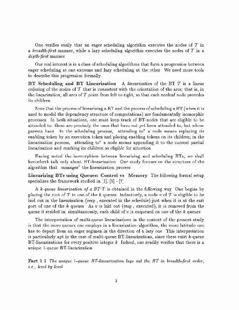
One veri�es easily that an eager scheduling algorithm executes the nodes of T ina breadth��rst manner� while a lazy scheduling algorithm executes the nodes of T in adepth��rst manner�

Our real interest is in a class of scheduling algorithms that form a progression betweeneager scheduling at one extreme and lazy scheduling at the other� We need more toolsto describe this progression formally�

BT Scheduling and BT Linearization� A linearization of the BT T is a linearordering of the nodes of T that is consistent with the orientation of the arcs� that is� inthe linearization� all arcs of T point from left to right� so that each nonleaf node precedesits children�

Note that the process of linearizing a BT and the process of scheduling a BT �when it isused to model the dependency structure of computations are fundamentally isomorphicprocesses� In both situations� one must keep track of BT�nodes that are eligible to beattended to� these are precisely the ones that have not yet been attended to� but whoseparents have� In the scheduling process� �attending to� a node means replacing itsenabling token by an execution token and placing enabling tokens on its children� in thelinearization process� �attending to� a node means appending it to the current partiallinearization and marking its children as eligible for attention�

Having noted the isomorphism between linearizing and scheduling BTs� we shallhenceforth talk only about BT�linearization� Our study focuses on the structure of thealgorithm that �manages� the linearization process�

Linearizing BTs using Queues� Control vs� Memory� The following formal setupspecializes the framework studied in �� � � ��

A k�queue linearization of a BT T is obtained in the following way� One begins byplacing the root of T in one of the k queues� Inductively� a node v of T is eligible to belaid out in the linearization �resp�� executed in the schedule just when it is at the exitport of one of the k queues� As v is laid out �resp�� executed � it is removed from thequeue it resided in� simultaneously� each child of v is enqueued on one of the k queues�

The interpretation of multi�queue linearizations in the context of the present studyis that the more queues one employs in a linearization algorithm� the more latitude onehas to depart from an eager regimen in the direction of a lazy one� This interpretationis particularly apt in the case of multi�queue BT�linearizations� since there exist k�queueBT�linearizations for every positive integer k� Indeed� one readily veri�es that there is aunique ��queue BT�linearization�

Fact ��� The unique ��queue BT�linearization lays out the BT in breadth��rst order�

i�e�� level by level�

�

A consequence of the rules for manipulating queues is that a BT�node does not entera queue until all of its ancestors have already left the queue� This veri�es the followingsimple observation� which is important later�

Fact ��� All nodes that coexist in the k queues at any instant must be independent inthe BT� i�e�� none is an ancestor of another�

Most obviously� the number of queues used for a particular BT�linearization is arelevant measure of the complexity of the control mechanism of the linearization algo�rithm used� No less relevant� though� is the question of the memory requirements of thealgorithm� as exposed by the individual and cumulative capacities of the queues thatimplement the algorithm� Speci�cally� the capacity of queue �q in the linearization al�gorithm is the maximum number of nodes of T that will ever reside in queue �q at thesame instant� The cumulative capacities of the queues is the sum of the capacities of theindividual queues� Our goal is to expose a tradeo� between the amount of control in alinearization algorithm and the memory requirements of the algorithm� We accomplishthis in the special case when the dag being linearized is a CBT� �Note� however� that ourlower bound applies to a broader class of BTs�

� A Control�Memory Tradeo�

For all positive integers N � �n and k � n� let Qk�N denote the minimum per�queue

capacity when k queues are used to linearize a CBT having N leaves� Dually� for allpositive integers k and Q� let N k�Q denote the maximum number of leaves in a CBT

that can be linearized using k queues� each of capacity Q� In order to avoid a proliferationof �oors and ceilings in our calculations� we assume henceforth that Q is a power of ��this assumption will be seen to a�ect only constant factors�

An immediate consequence of Fact ��� is the following tight speci�cation of Q��N �

Lemma ��� For all positive integers N � �n� Q��N � N���

We have already mentioned that our goal here is to establish a tradeo� between thecontrol complexity of a CBT�linearization algorithm � as measured by the quantity k� and the memory capacity of the algorithm � as measured by the quantity Qk�N �We �rst present �in Section ��� a simple family of CBT�linearization algorithms thatat least suggests that such a tradeo� exists� We then state �in Section ��� the actualtradeo�� with upper and lower bounds that are close to coincident� Sections � and � arethen devoted� respectively� to proving the upper and lower bounds of the tradeo��

�

��� A Recursive CBT�Linearization Algorithm

The possibility that there is a control�memory tradeo� for CBT�linearization algorithmsis suggested by the following simple family of algorithms� For notational simplicity� wheninvoking the k�queue version of the following family of algorithms� we assume that theheight of the input CBT is divisible by k�

A k�Queue CBT�Linearization Algorithm

Input� an �N � �n �leaf CBT T

�� Linearize the top n�k levels of T using queue �k�

�� For each �leaf� of the tree linearized in step �� in turn� linearize the CBT rooted atthat �leaf� by using queues �� � ��k� � recursively to execute the �k� � �queueversion of this algorithm�

See Figure �

Analyzing the Algorithm� Since each queue is used to linearize �possibly many CBT�s of height �logN �k� no queue needs have capacity greater than O�N��k � uni�formly in N and k� �The big�O is needed to compensate for rounding when k does notdivide n� As an immediate consequence� we have�

Fact ��� For all positive integers N � �n and k � n�

Qk�N � O�N��k � ��

uniformly in N and k�

��� The Real Control�Memory Tradeo�

The research described here was motivated by the possible tradeo� suggested in Fact���� i�e�� by the possibility that there are lower bounds that match the upper bounds�� � We have veri�ed that there is� indeed� a tradeo� between the quantities k andQk�N � but not exactly the one suggested in the Fact� One aspect of our tradeo� resultthat we found mildly surprising is that there is a k�queue linearization algorithm thathas smaller maximum per�queue capacity than the algorithm presented in Section ����Another surprising aspect is that we obtain upper and lower bounds on Qk�N that di�erby only the factor k����k� Speci�cally� we prove the following bounds in the next twosections�

�

n/k

(k−1)n/k

use queue #k

#1 − #(k−1)

use queues

Figure �� �a The unique ��queue layout of the height�h CBT� �b A capacity saving

��queue layout of the height�h CBT�

�

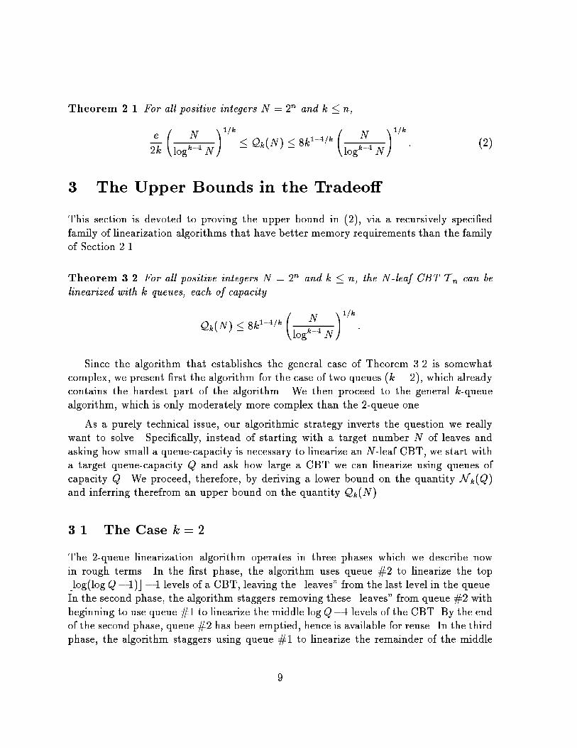
Theorem ��� For all positive integers N � �n and k � n�

e

�k

�N

logk��N

���k

� Qk�N � �k����k

�N

logk��N

���k

� ��

� The Upper Bounds in the Tradeo�

This section is devoted to proving the upper bound in �� � via a recursively speci�edfamily of linearization algorithms that have better memory requirements than the familyof Section ����

Theorem ��� For all positive integers N � �n and k � n� the N�leaf CBT T n can be

linearized with k queues� each of capacity

Qk�N � �k����k

�N

logk��N

���k

�

Since the algorithm that establishes the general case of Theorem ��� is somewhatcomplex� we present �rst the algorithm for the case of two queues �k � � � which alreadycontains the hardest part of the algorithm� We then proceed to the general k�queuealgorithm� which is only moderately more complex than the ��queue one�

As a purely technical issue� our algorithmic strategy inverts the question we reallywant to solve� Speci�cally� instead of starting with a target number N of leaves andasking how small a queue�capacity is necessary to linearize an N �leaf CBT� we start witha target queue�capacity Q and ask how large a CBT we can linearize using queues ofcapacity Q� We proceed� therefore� by deriving a lower bound on the quantity N k�Q and inferring therefrom an upper bound on the quantity Qk�N �

��� The Case k � �

The ��queue linearization algorithm operates in three phases which we describe nowin rough terms� In the �rst phase� the algorithm uses queue �� to linearize the topblog�logQ�� c�� levels of a CBT� leaving the �leaves� from the last level in the queue�In the second phase� the algorithm staggers removing these �leaves� from queue �� withbeginning to use queue �� to linearize the middle logQ�� levels of the CBT� By the endof the second phase� queue �� has been emptied� hence is available for reuse� In the thirdphase� the algorithm staggers using queue �� to linearize the remainder of the middle

�

log h −1

h−1

h

QUEUE #2

QUEUE #1QUEUE #1

#2 #2 #2 #2

Figure �� The target ��queue layout of the height�h CBT�

logQ� � levels of the CBT with using queue �� to linearize the bottom logQ� � levels�This latter staggering proceeds by having queue �� linearize a �logQ � � �level CBTrooted at each middle�tree �leaf� from queue ��� We then assess the size of the linearizedCBT as a function of the queue�capacity Q� To assist the reader in understanding theensuing technical details� we depict in Figure � the ultimate usage pattern of the twoqueues�

A� The E�cient ��Queue Linearization Algorithm

Phase �� The Top of the Tree�In this phase� we use queue �� to lay out the top blog�logQ� � c � � levels of the CBTwe are linearizing� using the breadth��rst regimen that is the unique way a single queue

��

TOP TREE

log log Q − 1

Last level:

NODES REMAINING IN QUEUE #2

Figure �� Laying out the top of the CBT�

can linearize a CBT� cf� Fact ���� At the end of this phase� queue �� will contain

�blog�logQ���c

nodes� We make the transition into Phase � of the algorithm by considering each of thesenodes in queue �� as the root of a �middle� CBT �which will have Q�� �leaves� � SeeFig� ��

Phase �� The Middle of the Tree�In this phase� we use queue �� to lay out themiddle trees that comprise the next logQ��levels of the CBT we are linearizing� This is the most complicated of the three phases�in that these middle trees get laid out in a staggered manner� in two senses� First� the�blog�logQ���c middle trees get interleaved in the linearization we are producing� Second�the layout of the middle trees is interleaved with segments of Phase �� wherein the bottomtrees are laid out�

We describe �rst the initial portion of Phase �� i�e�� the portion before the phase getsinterrupted by segments of Phase ��

Lay out the �rst node from queue ��� which is level � �i�e�� the root of the �rstmiddle tree� place the children of this node in queue ��� Next� proceed through thefollowing iterations� see Fig� ��

��

0 1

1 1 22

2 2 2 2

3 3 3 3 3 3 3 3

3 3 3 3

3 3

2

Figure �� The initial steps of Phase ��

��

Step �� Begin the �rst middle tree�

Step ���� Use queue �� to lay out level � of the �rst middle tree�

Step ���� Use queue �� to lay out level � of the second middle tree� placing thechildren of this root in queue ���

Step �� Continue the �rst middle tree� begin the second middle tree�

Step ���� Use queue �� to lay out level � of the �rst middle tree�

Step ���� Use queue �� to lay out level � of the second middle tree�

Step ���� Use queue �� to lay out level � of the third middle tree� placing thechildren of this root in queue ���

Step �� Continue the �rst and second middle trees� begin the third middle tree�

Step ���� Use queue �� to lay out level � of the �rst middle tree�

Step ���� Use queue �� to lay out level � of the second middle tree�

Step ���� Use queue �� to lay out level � of the third middle tree�

Step ���� Use queue �� to lay out level � of the fourth middle tree� placing thechildren of this root in queue ���

� � �Step �logQ� �� Finish the �rst middle tree� continue the second through next�to�last

middle trees� begin the last middle tree�

Step �logQ� ���� Use queue �� to lay out level logQ � � of the �rst middletree�

Step �logQ� ���� Use queue �� to lay out level logQ� � of the second middletree�

� � �Step �logQ� ���logQ� �� Use queue �� to lay out level � of the second from

last middle tree�

Step �logQ� ���logQ� �� Use queue �� to lay out level � of the last middletree� placing the children of this root in queue ���

At this point� queue �� has been completely emptied� hence is available for reuse�Queue ��� on the other hand� contains fewer than Q nodes� Speci�cally� queue ��contains Q�� nodes from the �rst middle tree� and� in general� it contains only half as

��

many node from the �i� � th middle tree as it does from the ith� in the worst case� ofcourse� there are

�blog�logQ���c � logQ� �

middle trees� hence Q� � nodes in queue ��� See Fig� ��

We have now completely laid out the �rst middle tree and partially laid out all theother middle trees� Ultimately� we shall continue to use queue �� in the same interleaved�power�of�� decreasing manner as described here� to lay out the remaining middle trees�First� though� we initiate Phase � in which queue �� is used to lay out the bottom levelsof the CBT being linearized� It is important to begin Phase � now� because some of thecontents of queue �� must be unloaded at this point� in order to make room for theremaining levels of the remaining middle trees�

Phase �� The Bottom of the Tree�Phase � is partitioned into two subphases� In the �rst of these subphases � call it Phase�a � we begin viewing the �leaves� of the middle trees as the roots of bottom trees �each being a CBT with N ��Q � �Q leaves� In the second of these subphases � call itPhase �b � we continue using the regimen of Phase � to lay out the middle trees�

Phase �a� This subphase is active whenever the nodes at the front of queue ��come from level logQ � � of a middle tree �which is the last level to enter queue �� �During the subphase� we iteratively lay out a single node � call it node v � from queue��� and we use queue �� to lay out a CBT on �Q leaves� rooted at node v �using thebreadth��rst regimen� of course � See Fig� ��

Phase �b� This subphase is active whenever the nodes at the front of queue �� do

not come from level logQ � � of a middle tree� During the subphase� we perform onemore step of Phase �� to extend the layout of the middle tree� To illustrate our intent� theinstance of Subphase �b that is executed immediately after the �rst round of executionsof Subphase �a �wherein the leftmost Q�� bottom trees are laid out has the form�

Step �logQ� �� Finish the second middle tree� continue the third through last middletrees�

Step �logQ� ���� Use queue �� to lay out level logQ� � of the second middletree�

Step �logQ� ���� Use queue �� to lay out level logQ � � of the third middletree�

� � �Step �logQ� ���logQ� �� Use queue �� to lay out level � of the second from

last middle tree�

��

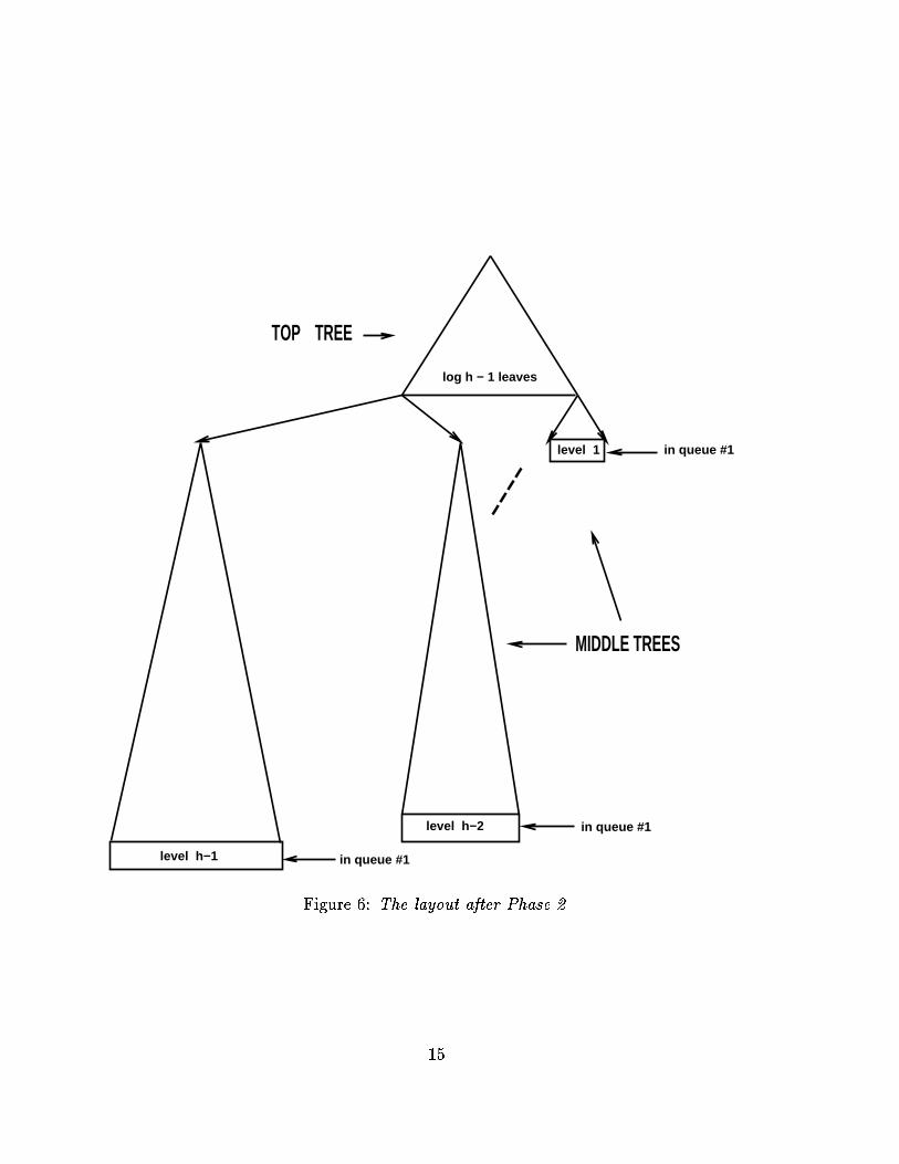
TOP TREE

MIDDLE TREES

level h−1

level h−2

level 1

log h − 1 leaves

in queue #1

in queue #1

in queue #1

Figure �� The layout after Phase ��

��

TOP TREE

BOTTOM TREES

MIDDLE TREES

level h−2

level h−1

(h levels each)

level 1

log h − 1 leaves

in queue #1

in queue #1

in queue #1

Figure �� The layout after Phase �a begins the �rst two bottom trees have been laid out�

��

Step �logQ� ���logQ� �� Use queue �� to lay out level � of the last middletree�

See Fig� ��

B� The Analysis

Correctness being �hopefully clear� we need only see how much CBT we are getting forgiven queue�capacity Q� There are

�blog�logQ���c ��

��logQ� �

top�tree leaves� hence� at least ��Q�logQ�� middle�tree leaves� hence at least �

�Q��logQ�

� CBT leaves� It follows that

N ��Q � �

�Q��logQ� � �

Inverting this inequality to obtain the desired upper bound on Q��N � we �nd that

Q��N � �p�

�N

logN

����

�

��� The Case of General k

We now show how to generalize the ��queue algorithm to a family of algorithms forarbitrary numbers of queues�

A� The Algorithm

Our general linearization algorithm uses Phases �� �� and �b of the ��queue algorithmdirectly� It modi�es only Phase �a� as follows�

Phase �a� This subphase is active whenever the nodes at the front of queue ��come from level logQ � � of a middle tree �which is the last level to enter queue �� �During the subphase� we iteratively lay out a single node � call it node v � from queue��� and we use queues �� � �k to lay out a CBT on �Q leaves� rooted at node v� usinga recursive invocation of the �k � � �queue version of this algorithm�

Note that the ��queue algorithm of the previous subsection can� in fact� be obtainedvia this recursive strategy� from the base case k � ��

As we did earlier� we remark that queues �� � �k are all available for this recursivecall because� �a queue �� lays out the last �leaf� of the top tree just before queue ��

��

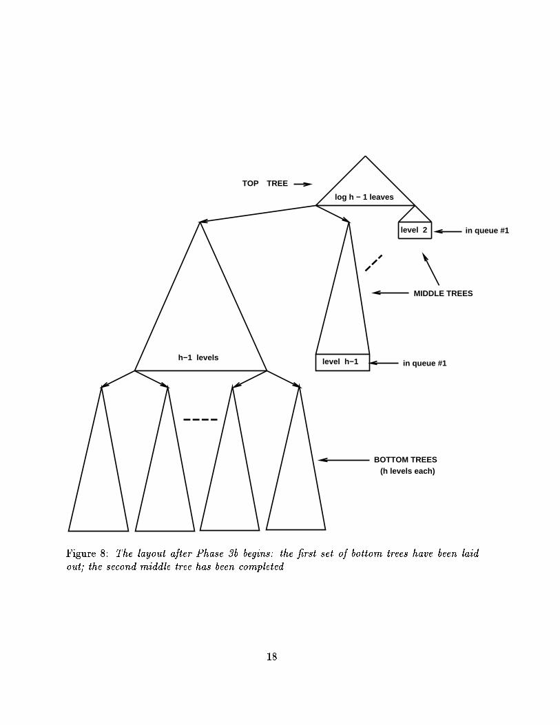
TOP TREE

BOTTOM TREES

MIDDLE TREES

h−1 levels level h−1

level 2

log h − 1 leaves

(h levels each)

in queue #1

in queue #1

Figure �� The layout after Phase �b begins the �rst set of bottom trees have been laid

out� the second middle tree has been completed�

��

lays out the �rst �leaf� of the leftmost middle tree� so it is available� �b queues �� � �kare not used at all with the top or middle trees above this level of the �nal CBT�

B� The Analysis

Correctness being �hopefully obvious� we need consider only how many leaves the CBTwe have generated has� as a function of the given queue�capacity Q� This number iseasily seen to be be given by the recursion

N ��Q � �Q

N k���Q � �

�Q�logQ� � N k�Q

Easily� this yields the following solution� which holds for all k � ��

N k�Q � �Q��

�Q logQ

�k��

�

For our ends� we invert this relation� to get the sought upper bound on Qk�N � namely�

Qk�N � �k����k

�N

logk��N

���k

�

This completes the proof� � To wit�

N � ����kQk logk��Q

so thatlogN � k logQ

so that

Qk � ����kkk�� N

logk��N�

� The Lower Bounds in the Tradeo�

This section is devoted to proving the lower bound in Theorem ���� In fact� we provethis bound as a corollary of the following more general lower bound�

Theorem ��� For all positive integers N � �n and k � n� given any k�queue lineariza�

tion of a BT having width N and c logN levels� at least one queue must have capacity at

least

e

�ck

�N

logk��N

���k

�

��

Corollary ��� For all positive integers N � �n and k � n� given any k�queue lineariza�

tion of the N�leaf CBT� at least one of the queues must have capacity

Qk�N � e

�k

�N

logk��N

���k

�

Proof of Theorem ���� Say that we are given an arbitrary k�queue linearization of aBT T having width N and c logN levels �for some constant c � � � Call a level of Tthat has N nodes a wide level�

We begin by parsing the given linearization into contiguous substrings� by partitioningthe linearization process into phases� For the purpose of de�ning the phases� recall thatthe action of laying out a node �i�e�� appending it to the current partial linearization and loading its children into queues is a single atomic action�

De�ne Phase � to be that part of the process wherein the root of T �which must bethe �rst node laid out is laid out and its children loaded on queues� Hence� the �rstsubstring in the parsing is just a one�letter string consisting of the root�

Inductively� de�ne Phase i � � to be that part of the process wherein all nodes thatwere loaded into queues during Phase i are laid out� the Phase ends when the last ofthese Phase�i �legacies� has been laid out� The substring produced during Phase i� �is� then� the longest substring following the substring produced during Phase i� duringwhich some queue still contains a node that was put there during Phase i�

By a straightforward induction� one establishes that level i of the BT T must be laidout by the end of Phase i� It follows that

Fact ��� There are at most c logN phases in the linearization process�

Fact ��� has the following immediate consequence�

Fact �� There must exist a phase whose associated substring contains at least N��c logN nodes from a wide level of T � Call such a phase long�

Now look at what happens during a phase of an optimal linearization of T � i�e�� onethat minimizes the capacity of the largest�capacity queue� The phase starts with somenodes residing within the k queues � at most Qk�N per queue� As we noted in Fact ����all of these nodes must be independent in the BT� Moreover� by de�nition of �phase�� allof these nodes must be laid out by the end of the phase� We can� therefore� characterizewhat the portion of T that is laid out during a phase looks like�

��

Fact ��� What is laid out during a phase is a forest of BTs rooted at the � kQk�N nodes that resided in the queues at the start of the phase�

Note now that some BT � call it T � � in the forest laid out during a long phasemust contain as nodes at least N��ckQk�N logN of the nodes from the wide level ofT � Hence� the width of T � can be no smaller than this quantity�

Fact ��� At least one of the BTs in the forest must have width no smaller than

N

ckQk�N logN�

Next note that� by de�nition of �phase�� there must be some queue � call it queue�m � whose sole contributions to the linearization during the long phase are the nodesthat started in it at the beginning of the phase� This is because the phase ends whenthe last node that was created during the previous phase is laid out � so queue �mis identi�ed as the source of this last node� Now� queue �m started the phase �as didevery queue with no more than Qk�N nodes� As we noted earlier� each of these nodesis the root of a BT generated during the long phase� Of all the nodes laid out during thelong phase� only these roots come from queue �m� Now� if we remove from the forestall these queue��m nodes� then we partition each BT T �� that is rooted at a queue��mnode into two BTs� at least one of which must have at least half the width of T ��� Itfollows� therefore� that

Fact �� The forest generated during the long phase must� after all queue��m nodes are

removed� contain a BT of width no smaller than

N

�ckQk�N logN

that is generated by only k � � of the queues�

We infer immediately the recurrent lower bound

Qk�N � Qk��

�N

�ckQk�N logN

���

whose initial case �k � � is resolved in Lemma ��� �for the case of a CBT �

We solve recurrence �� by induction� making two assumptions� First� we assume forinduction that

Qk���N � �k��

�N

logk��N

����k���

��

��

for some quantity �k�� which will be determined later �although we already know fromLemma ��� that �� � ��� when T is an N �leaf CBT � Second� we assume that

logQk�N ��

klogN � l�o�t��

This assumption will turn out to be easy to verify�

We begin by substituting inequality �� into recurrence �� � to obtain

Qk�N � �k��

��� N

�ckQk�N logN

��k

�k � � logN

�k���A

���k���

� ��

After some manipulation� inequality �� becomes

Qk�N ��

kk��

�c�k � � k��

���k

��k����kk��

�N

logk��N

���k

� ��

In order to obtain the desired lower bound� we now turn our attention to the followingrecurrence� which is suggested by inequality �� �

�k �

�kk��

�c�k � � k��

���k

��k����kk�� � ��

with initial condition �� � ���� Elementary manipulation converts recurrence �� to therecurrent bound

�k ��

�

�ck

���k �� �

�

k � �

���k

��k����kk�� �

��

�ck

���k

��k����kk�� �

so that

�k � �

�c

��

k�

���k�

e

�ck� ��

Combining inequality �� with inequality �� via recurrence �� yields the lower boundof Theorem ���� �

Proof of Corollary ���� The lower bound of Corollary ��� is immediate from that ofTheorem ��� if one notes that the N �leaf CBT has logN � � levels �so c � � � �

Remark� A more careful analysis replaces the recurrent bound �� by

Qk�N � Qk��

�N

c�k � � Qk�N logN�Qk�N

��

��

which solves to a marginally larger lower bound �by a constant factor � The reasoningbehind this better recurrence is as follows� If we remove the nodes that came from queue�m� we have left � �k � � Qk�N trees� each of which is generated by only k � � of thequeues� Since each of the nodes that came from queue �m could� in fact� come from awide level of the big BT� removing these nodes could decrease the number of wide�levelnodes laid out during this phase by � Qk�N � What this means is�

Fact ��� During a phase whose substring contains L nodes from a wide level of the BT

T � there must be a BT of width at least

L

c�k � � Qk�N �Qk�N

that is generated by only k � � of the queues�

ACKNOWLEDGMENTS� The authors thank Marc Snir for helpful comments in theearly stages of this research and Li�Xin Gao for helpful discussions in the later stages�

The research of S� N� Bhatt was supported in part by NSF Grants MIP��������� andCCR���������� by NSF�DARPA Grant CCR���������� and by Air Force Grant AFOSR��������� the research of F� T� Leighton was supported in part by Air Force Contract OSR��������� DARPA Contract N���������C������ Army Contract DAAL�������K������ andNSF Presidential Young Investigator Award with matching funds from ATT and IBM�the research of A� L� Rosenberg was supported in part by NSF Grant CCR���������� Aportion of this research was done while S� N� Bhatt� F� T� Leighton� and A� L� Rosenbergwere visiting Bell Communications Research�

References

� A�T� Barrett� L�S� Heath� and S�V� Pemmaraju ����� � Stack and queue layouts ofdirected acyclic graphs� ��� DIMACS Workshop on Planar Graphs Structure and

Algorithms� to appear�

� A� Gerasoulis and T� Yang ����� � A comparison of clustering heuristics for schedul�ing dags on multiprocessors� J� Parallel and Distr� Comput�

� A� Gerasoulis and T� Yang ����� � Scheduling program task graphs on MIMD ar�chitectures� Typescript� Rutgers Univ�

��

� A� Gerasoulis and T� Yang ����� � Static scheduling of parallel programs for messagepassing architectures� Parallel Processing CONPAR �� � VAPP V� Lecture Notes

in Computer Science ��� Springer�Verlag� Berlin�

� L�S� Heath� F�T� Leighton� A�L� Rosenberg ����� � Comparing queues and stacksas mechanisms for laying out graphs� SIAM J� Discr� Math� �� ��������

� L�S� Heath and S�V� Pemmaraju ����� � Stack and queue layouts of posets� Tech�Rpt� ������ VPI�

� L�S� Heath and A�L� Rosenberg ����� � Laying out graphs using queues� SIAM J�

Comput� �� ��������

� S�J� Kim and J�C� Browne ����� � A general approach to mapping of parallel com�putations upon multiprocessor architectures� Intl� Conf� on Parallel Processing ������

� M� Litzkow� M� Livny� M� Matka ����� � Condor � A hunter of idle workstations��th Ann� Intl� Conf� on Distributed Computing Systems�

�� D� Nichols ����� � Multiprocessing in a Network of Workstations� Ph�D� thesis�CMU�

�� C�H� Papadimitriou and M� Yannakakis ����� � Towards an architecture�independent analysis of parallel algorithms� SIAM J� Comput� �� ��������

�� S�W� White and D�C� Torney ����� � Use of a workstation cluster for the physicalmapping of chromosomes� SIAM NEWS� March� ����� ������

�� J� Yang� L� Bic� A� Nicolau ����� � A mapping strategy for MIMD computers� Intl�Conf� on Parallel Processing � ��������

�� T� Yang and A� Gerasoulis ����� � A fast static scheduling algorithm for dags onan unbounded number of processors� Supercomputing ��� ��������

�� T� Yang and A� Gerasoulis ����� � PYRROS� static task scheduling and code gen�eration for message passing multiprocessors� th ACM Conf� on Supercomputing���������

��