scalability engineering for parallel programs using empirical performance … · 2018-06-16 ·...
TRANSCRIPT

Scalability Engineering forParallel Programs UsingEmpirical Performance ModelsEntwicklung skalierbarer paralleler Programme mittels empirischerPerformance-ModelleZur Erlangung des akademischen Grades Doktor-Ingenieur (Dr.-Ing.)genehmigte Dissertation von Sergei Shudler, M.Sc. aus Jekaterinburg, RusslandTag der Einreichung: 29.01.2018, Tag der Prüfung: 16.04.2018Darmstadt — 2018 — D 17
1. Gutachten: Prof. Dr. Felix Wolf2. Gutachten: Prof. Dr. Martin Schulz
Fachbereich InformatikLaboratory for Parallel Programming

Scalability Engineering for Parallel Programs Using Empirical Performance ModelsEntwicklung skalierbarer paralleler Programme mittels empirischer Performance-Modelle
Genehmigte Dissertation von Sergei Shudler, M.Sc. aus Jekaterinburg, Russland
1. Gutachten: Prof. Dr. Felix Wolf2. Gutachten: Prof. Dr. Martin Schulz
Tag der Einreichung: 29.01.2018Tag der Prüfung: 16.04.2018
Darmstadt — 2018 — D 17
Bitte zitieren Sie dieses Dokument als:URN: urn:nbn:de:tuda-tuprints-74714URL: http://tuprints.ulb.tu-darmstadt.de/7471
Dieses Dokument wird bereitgestellt von tuprints,E-Publishing-Service der TU DarmstadtJahr der Veröffentlichung der Dissertation auf TUprints: 2018http://[email protected]
Die Veröffentlichung steht unter folgender Creative Commons Lizenz:Namensnennung – Keine kommerzielle Nutzung – Keine Bearbeitung 4.0 Internationalhttps://creativecommons.org/licenses/by-nc-nd/4.0/

Tomy parents


Erklärung zur Dissertation
Hiermit versichere ich, die vorliegende Dissertation ohne Hilfe Dritter nur mitden angegebenen Quellen und Hilfsmitteln angefertigt zu haben. Alle Stellen, dieaus Quellen entnommen wurden, sind als solche kenntlich gemacht. Diese Arbeithat in gleicher oder ähnlicher Form noch keiner Prüfungsbehörde vorgelegen.
Darmstadt, den 29.01.2018
(Sergei Shudler)
iii


AbstractPerformance engineering is a fundamental task in high-performance computing (HPC). By defi-nition, HPC applications should strive for maximum performance. As HPC systems grow largerand more complex, the scalability of an application has become of primary concern. Scalabilityis the ability of an application to show satisfactory performance even when the number of pro-cessors or the problems size is increased. Although various analysis techniques for scalabilitywere suggested in past, engineering applications for extreme-scale systems still occurs ad hoc.The challenge is to provide techniques that explicitly target scalability throughout the wholedevelopment cycle, thereby allowing developers to uncover bottlenecks earlier in the develop-ment process. In this work, we develop a number of fundamental approaches in which we useempirical performance models to gain insights into the code behavior at higher scales.
In the first contribution, we propose a new software engineering approach for extreme-scalesystems. Specifically, we develop a framework that validates asymptotic scalability expectationsof programs against their actual behavior. The most important applications of this method,which is especially well suited for libraries encapsulating well-studied algorithms, include ini-tial validation, regression testing, and benchmarking to compare implementation and platformalternatives. We supply a tool-chain that automates large parts of the framework, thus allowingit to be continuously applied throughout the development cycle with very little effort. We eval-uate the framework with MPI collective operations, a data-mining code, and various OpenMPconstructs. In addition to revealing unexpected scalability bottlenecks, the results also showthat it is a viable approach for systematic validation of performance expectations.
As the second contribution, we show how the isoefficiency function of a task-based programcan be determined empirically and used in practice to control the efficiency. Isoefficiency, aconcept borrowed from theoretical algorithm analysis, binds efficiency, core count, and the in-put size in one analytical expression, thereby allowing the latter two to be adjusted accordingto given (realistic) efficiency objectives. Moreover, we analyze resource contention by model-ing the efficiency of contention-free execution. This allows poor scaling to be attributed eitherto excessive resource contention overhead or structural conflicts related to task dependenciesor scheduling. Our results, obtained with applications from two benchmark suites, demon-strate that our approach provides insights into fundamental scalability limitations or excessiveresource overhead and can help answer critical co-design questions.
Our contributions for better scalability engineering can be used not only in the traditionalsoftware development cycle, but also in other, related fields, such as algorithm engineering. Itis a field that uses the software engineering cycle to produce algorithms that can be utilizedin applications more easily. Using our contributions, algorithm engineers can make informeddesign decisions, get better insights, and save experimentation time.
v


ZusammenfassungPerformance Engineering ist eine grundlegende Aufgabe im Hochleistungsrechnen (HPC).Der Definition gemäß sollten HPC-Anwendungen nach maximaler Leistung streben. Da HPC-Systeme immer größer und komplexer werden, ist auch die Skalierbarkeit einer Anwendung zueinem der Hauptanliegen geworden. Skalierbarkeit beschreibt die Fähigkeit einer Anwendung,eine zufriedenstellende Leistung zu erzielen, selbst wenn die Anzahl der Prozessoren oder dasAusmaß der Probleme sich erhöht. Obwohl schon vor geraumer Zeit verschiedene Analyse-techniken zur Skalierbarkeit vorgeschlagen wurden, erfolgt die Entwicklung von Anwendungenfür extrem skalierbare Systeme immer noch ad hoc. Die Herausforderung dabei ist, Technikenbereitzustellen, die explizit auf eine Skalierbarkeit über den gesamten Entwicklungszyklus ab-zielen und somit den Entwicklern ermöglichen, Mängel am Entwicklungsprozess frühzeitig zuerkennen. In dieser Arbeit entwickeln wir eine Reihe von grundlegenden Ansätzen, in denen wirempirische Performance-Modelle verwenden, um Einblicke in das Code-Verhalten bei höhererSkalierung zu erhalten.
Im ersten Beitrag schlagen wir einen neuen Ansatz zur Softwareentwicklung für Systeme mitextremer Skalierbarkeit vor. Insbesondere entwickeln wir hier ein Framework, das asymptoti-sche Skalierbarkeitserwartungen von Programmen mit ihrem tatsächlichen Verhalten vergleichtund bewertet. Die wichtigsten Anwendungen für diese Methode, welche sich besonders gut fürBibliotheken mit gut erforschten Algorithmen eignet, umfassen u. a. Erstvalidierung, Regres-sionstests und Benchmarking zum Vergleich von Implementierung und Plattformalternativen.Wir stellen etliche Werkzeuge bereit, die einen Großteil des Frameworks automatisieren undes somit ermöglichen, dieses ohne großen Aufwand während des gesamten Entwicklungszyklusanzuwenden. Wir evaluieren das Framework mit kollektiven MPI-Maßnahmen, einem Data-Mining-Code und diversen OpenMP-Konstrukten. Neben der Enthüllung unerwarteter Skalier-barkeitsengpässe zeigen die Ergebnisse auch, dass es sich hier um einen realisierbaren Ansatzzur systematischen Validierung von Performance-Erwartungen handelt.
Als zweiten Beitrag zeigen wir, wie die Isoeffizienzfunktion eines aufgabenbasierten Pro-gramms empirisch bestimmt und in der Praxis zur Effizienzkontrolle genutzt werden kann.Bei der Isoeffizienz handelt es sich um ein aus der theoretischen Algorithmenanalyse entlehntesKonzept. Es verbindet Effizienz, Kernanzahl und Eingabegröße zu einem analytischen Ausdruck,wodurch letztere zwei Werte gemäß vorgegebenen (realistischen) Effizienzzielen angepasstwerden. Außerdem analysieren wir Ressourcenkonflikte, indem wir die Effizienz einer kon-fliktfreien Ausführung modellieren. Dadurch wird ermöglicht, schlechte Skalierungen entwederexzessivem Aufwand auf Grund von Ressourcenkonflikten oder Strukturkonflikten zuzuordnen,die auf Aufgabenabhängigkeiten oder Planungen zurückzuführen ist. Unsere Ergebnisse, diemit Anwendungen aus zwei Benchmark-Suites ermittelt wurden, zeigen, dass unser Ansatz Ein-blicke in grundlegende Skalierbarkeitsbeschränkungen oder exzessiven Ressourcenverbrauchbereitstellt und helfen kann, Antworten auf wichtige Co-Design-Fragen zu finden.
Unsere Beiträge zur Verbesserung der Skalierbarkeitsentwicklungen können nicht nur für dentraditionellen Softwareentwicklungszyklus verwendet werden, sondern auch für andere geeig-nete Forschungsfelder, z. B. Algorithmenentwicklung. Dabei handelt es sich um ein Feld, indem der Softwareentwicklungszyklus dazu genutzt wird, Algorithmen zu entwickeln, die spä-ter einfacher in Anwendungen verwendet werden können. Durch Verwendung unserer Beiträgekönnen Algorithmenentwickler fundierte Designentscheidungen treffen, bessere Einblicke er-halten und beim Experimentieren Zeit sparen.
vii


AcknowledgmentsCompleting a PhD program is akin to traveling through a deep forest without a trail – yousee the entrance, but you have no idea where eventually you exit the forest and how long thejourney will take. For me, this path towards completion was not always easy and not alwaysclear. But it was always exciting, and never ceased to present new challenges that would spurfurther professional and personal growth. I would like to the acknowledge the people whomade this journey easier and more joyful.
First and foremost, my deepest gratitude goes to my doctoral advisor Prof. Dr. Felix Wolf,who provided me with the opportunity to work on cutting-edge research. His guidance andsupport allowed me to develop myself as a researcher. Without Prof. Wolf’s immense help anddedication this work would not have been possible.
I would also like to express my sincere appreciation and gratitude to Prof. Dr. Torsten Hoefler.Prof. Hoefler’s inspiring passion and ideas motivated me to continue even at times when thepath ahead was unclear. The collaboration with Prof. Hoefler and his suggestions proved to beinvaluable. I also wish to express gratitude to Prof. Dr. Martin Schulz, who provided me withthe opportunity to do an internship at Lawrence Livermore National Laboratory (LLNL). Prof.Schulz mentored me throughout the internship and encouraged me to pursue new directions inmy work. The stay at LLNL was both fruitful and enjoyable.
I wish to thank all the people in the Laboratory for Parallel Programming at Technische Uni-versität Darmstadt. A special thank goes to Dr. Alexandru Calotoiu for helpful discussions andsuggestions. Without the techniques he developed this work would probably not materialize. Ialso wish to thank Sebastian Rinke for being a good friend and for all the sport activities we didtogether, as well as thank Petra Stegmann for her indispensable help with administrative issues.I would also like to acknowledge the help of Dr. Daniel Lorenz.
Finally, I would like to thank my family—my parents and my sister—for supporting methroughout the years.
ix


Contents
List of Figures xiii
List of Tables xv
1 Introduction 11.1 High-Performance Computing . . . . . . . . . . . . . . . . . . . . . . . . . . . . . . . . 1
1.1.1 Supercomputer architecture . . . . . . . . . . . . . . . . . . . . . . . . . . . . . 21.1.2 Exascale . . . . . . . . . . . . . . . . . . . . . . . . . . . . . . . . . . . . . . . . . 5
1.2 Parallel Programming . . . . . . . . . . . . . . . . . . . . . . . . . . . . . . . . . . . . . . 61.2.1 Shared-memory paradigm . . . . . . . . . . . . . . . . . . . . . . . . . . . . . . 81.2.2 Message-passing paradigm . . . . . . . . . . . . . . . . . . . . . . . . . . . . . . 11
1.3 Performance Analysis and Engineering . . . . . . . . . . . . . . . . . . . . . . . . . . . 151.3.1 Observation . . . . . . . . . . . . . . . . . . . . . . . . . . . . . . . . . . . . . . . 161.3.2 Analysis . . . . . . . . . . . . . . . . . . . . . . . . . . . . . . . . . . . . . . . . . 171.3.3 Performance modeling . . . . . . . . . . . . . . . . . . . . . . . . . . . . . . . . 19
1.4 Motivation and Scope . . . . . . . . . . . . . . . . . . . . . . . . . . . . . . . . . . . . . 191.5 Dissertation Contributions . . . . . . . . . . . . . . . . . . . . . . . . . . . . . . . . . . . 201.6 Dissertation Structure . . . . . . . . . . . . . . . . . . . . . . . . . . . . . . . . . . . . . 21
2 Empirical Performance Modeling 232.1 Overview . . . . . . . . . . . . . . . . . . . . . . . . . . . . . . . . . . . . . . . . . . . . . 232.2 Performance Model Normal Form . . . . . . . . . . . . . . . . . . . . . . . . . . . . . . 242.3 Model Generation . . . . . . . . . . . . . . . . . . . . . . . . . . . . . . . . . . . . . . . . 25
2.3.1 Automated refinement algorithm . . . . . . . . . . . . . . . . . . . . . . . . . . 262.3.2 Segmented regression . . . . . . . . . . . . . . . . . . . . . . . . . . . . . . . . . 272.3.3 Application examples . . . . . . . . . . . . . . . . . . . . . . . . . . . . . . . . . 28
2.4 Extra-P . . . . . . . . . . . . . . . . . . . . . . . . . . . . . . . . . . . . . . . . . . . . . . . 282.5 Multi-parameter Modeling . . . . . . . . . . . . . . . . . . . . . . . . . . . . . . . . . . . 31
2.5.1 Extended performance model normal form . . . . . . . . . . . . . . . . . . . . 312.5.2 Optimization techniques . . . . . . . . . . . . . . . . . . . . . . . . . . . . . . . 312.5.3 Application examples . . . . . . . . . . . . . . . . . . . . . . . . . . . . . . . . . 31
2.6 Summary and Outlook . . . . . . . . . . . . . . . . . . . . . . . . . . . . . . . . . . . . . 32
3 Scalability Validation of HPC Libraries 353.1 Approach Overview . . . . . . . . . . . . . . . . . . . . . . . . . . . . . . . . . . . . . . . 353.2 Scalability Validation Framework . . . . . . . . . . . . . . . . . . . . . . . . . . . . . . 37
3.2.1 Define expectations . . . . . . . . . . . . . . . . . . . . . . . . . . . . . . . . . . 373.2.2 Design benchmark . . . . . . . . . . . . . . . . . . . . . . . . . . . . . . . . . . . 383.2.3 Generate scaling models . . . . . . . . . . . . . . . . . . . . . . . . . . . . . . . 393.2.4 Validate expectations . . . . . . . . . . . . . . . . . . . . . . . . . . . . . . . . . 41
3.3 Case Study: MPI Collective Operations . . . . . . . . . . . . . . . . . . . . . . . . . . . 423.3.1 Scalability validation workflow . . . . . . . . . . . . . . . . . . . . . . . . . . . 423.3.2 Evaluation . . . . . . . . . . . . . . . . . . . . . . . . . . . . . . . . . . . . . . . . 463.3.3 Intel MPI and Open MPI . . . . . . . . . . . . . . . . . . . . . . . . . . . . . . . 53
xi

3.4 Further Evaluation of the Validation Framework . . . . . . . . . . . . . . . . . . . . . 563.4.1 MAFIA . . . . . . . . . . . . . . . . . . . . . . . . . . . . . . . . . . . . . . . . . . 573.4.2 OpenMP . . . . . . . . . . . . . . . . . . . . . . . . . . . . . . . . . . . . . . . . . 583.4.3 Parallel sorting algorithms . . . . . . . . . . . . . . . . . . . . . . . . . . . . . . 61
3.5 Summary and Conclusion . . . . . . . . . . . . . . . . . . . . . . . . . . . . . . . . . . . 66
4 Task Dependency Graphs 694.1 Graph Abstraction for Task-based Applications . . . . . . . . . . . . . . . . . . . . . . 69
4.1.1 Metrics and rules . . . . . . . . . . . . . . . . . . . . . . . . . . . . . . . . . . . . 704.2 Graph Construction . . . . . . . . . . . . . . . . . . . . . . . . . . . . . . . . . . . . . . . 71
4.2.1 OmpSs . . . . . . . . . . . . . . . . . . . . . . . . . . . . . . . . . . . . . . . . . . 714.2.2 OpenMP Tools Interface . . . . . . . . . . . . . . . . . . . . . . . . . . . . . . . . 724.2.3 Libtdg tool . . . . . . . . . . . . . . . . . . . . . . . . . . . . . . . . . . . . . . . . 75
4.3 Graph Analysis . . . . . . . . . . . . . . . . . . . . . . . . . . . . . . . . . . . . . . . . . . 784.3.1 Critical path . . . . . . . . . . . . . . . . . . . . . . . . . . . . . . . . . . . . . . . 784.3.2 Maximum degree of concurrency . . . . . . . . . . . . . . . . . . . . . . . . . . 80
4.4 Task Replay Engine . . . . . . . . . . . . . . . . . . . . . . . . . . . . . . . . . . . . . . . 824.4.1 OmpSs runtime . . . . . . . . . . . . . . . . . . . . . . . . . . . . . . . . . . . . . 834.4.2 LLVM OpenMP runtime . . . . . . . . . . . . . . . . . . . . . . . . . . . . . . . . 85
4.5 Summary and Conclusion . . . . . . . . . . . . . . . . . . . . . . . . . . . . . . . . . . . 86
5 Practical Isoefficiency Analysis 875.1 Speedup and Efficiency Challenges . . . . . . . . . . . . . . . . . . . . . . . . . . . . . 875.2 Isoefficiency Analysis . . . . . . . . . . . . . . . . . . . . . . . . . . . . . . . . . . . . . . 895.3 Modeling Approach . . . . . . . . . . . . . . . . . . . . . . . . . . . . . . . . . . . . . . . 91
5.3.1 Modeling workflow . . . . . . . . . . . . . . . . . . . . . . . . . . . . . . . . . . 925.3.2 Multi-parameter modeling with Extra-P . . . . . . . . . . . . . . . . . . . . . . 93
5.4 Evaluation . . . . . . . . . . . . . . . . . . . . . . . . . . . . . . . . . . . . . . . . . . . . 935.4.1 Experimentation setup . . . . . . . . . . . . . . . . . . . . . . . . . . . . . . . . 945.4.2 Analysis of the results . . . . . . . . . . . . . . . . . . . . . . . . . . . . . . . . . 95
5.5 Summary and Conclusion . . . . . . . . . . . . . . . . . . . . . . . . . . . . . . . . . . . 102
6 Related Work 1036.1 Scalability Validation Framework . . . . . . . . . . . . . . . . . . . . . . . . . . . . . . 1036.2 Isoefficiency Analysis . . . . . . . . . . . . . . . . . . . . . . . . . . . . . . . . . . . . . . 104
7 Conclusions and Outlook 107
xii

List of Figures
1.1 The architecture of the IBM Blue Gene/Q system (taken from IBM Redbooksseries [6]). . . . . . . . . . . . . . . . . . . . . . . . . . . . . . . . . . . . . . . . . . . . . 2
1.2 Microprocessor trends in the last 45 years (data processed and provided by K.Rupp [14]). Single-thread performance is represented by the results of theSpecINT benchmarks [15], that is the ratio of the benchmark execution timeto a reference time. . . . . . . . . . . . . . . . . . . . . . . . . . . . . . . . . . . . . . . . 4
1.3 Fork-join parallelism. The master thread forks worker threads at three parallelregions and all the threads join back to a single thread to resume sequentialexecution. . . . . . . . . . . . . . . . . . . . . . . . . . . . . . . . . . . . . . . . . . . . . . 9
1.4 Simple “Hello World” code using OpenMP. . . . . . . . . . . . . . . . . . . . . . . . . . 101.5 Simple "Hello World" code using MPI. . . . . . . . . . . . . . . . . . . . . . . . . . . . . 111.6 Performance engineering cycle of applications in HPC. . . . . . . . . . . . . . . . . . 151.7 Examples of common performance analysis tools. . . . . . . . . . . . . . . . . . . . . 18
2.1 Workflow of scalability-bug detection proposed by Calotoiu et al. [43] that canbe generalized to empirical performance modeling in general. Dashed arrowsindicate optional paths taken after user decisions. . . . . . . . . . . . . . . . . . . . . 24
2.2 Iterative model construction process (taken from Calotoiu et al. [46]). . . . . . . . 272.3 Example of Extra-P’s plaintext format for performance experiments. . . . . . . . . . 292.4 The graphical user interface of Extra-P based on PyQt. . . . . . . . . . . . . . . . . . 292.5 The dialog in which a set of performance profiles can be provided as an input to
Extra-P. . . . . . . . . . . . . . . . . . . . . . . . . . . . . . . . . . . . . . . . . . . . . . . 30
3.1 Software development cycle with empirical performance modeling. . . . . . . . . . 363.2 Scalability validation framework overview including use cases. . . . . . . . . . . . . 373.3 Search space boundaries and deviation limits relative to the expectation E(x). . . 393.4 JuBE workflow (taken from Wolf et al. [47]). . . . . . . . . . . . . . . . . . . . . . . . 453.5 Measurements (circles, squares, triangles) and generated runtime models (plot
lines) on Juqueen, Juropa, and Piz Daint. . . . . . . . . . . . . . . . . . . . . . . . . . 513.6 Measurements (circles, squares, triangles) and generated MPI memory consump-
tion models (plot lines) on Juqueen, Juropa, and Piz Daint. . . . . . . . . . . . . . . 533.7 Measurements (circles, squares) and generated runtime models (plot lines) of
some of the collective operations in Intel MPI and Open MPI. . . . . . . . . . . . . . 553.8 Parallel sorting based on finding exact splitters (from Siebert and Wolf [97]). . . . 62
4.1 Task dependency graph; each node contains the task time and the highlightedtasks form the critical path. . . . . . . . . . . . . . . . . . . . . . . . . . . . . . . . . . . 70
4.2 Task dependency graph produced by the Nanos++ TDG plugin. . . . . . . . . . . . 724.3 Example of Libtdg usage. . . . . . . . . . . . . . . . . . . . . . . . . . . . . . . . . . . . 75
xiii

4.4 Task dependency graph produced by the Libtdg tool that represents the executionof a simple matrix multiplication code with one parallel loop on one thread. Thegreen-colored node represents the beginning of a parallel loop and its childrenare loop chunks. The numbers in each node before the asterisk (*) are the exe-cution times in seconds. The numbers after it are either node IDs or the iterationranges of the loop chunks. . . . . . . . . . . . . . . . . . . . . . . . . . . . . . . . . . . . 76
4.5 Task dependency graph produced by the Libtdg tool that represents the execu-tion of a simple matrix multiplication code with one parallel loop on two threads.Each green-colored node, which represents the beginning of a parallel loop, cor-responds to a different thread. The children nodes of a green-colored node areloop chunks. The numbers in each node before the asterisk (*) are the executiontimes in seconds. The numbers after it are either node IDs or the iteration rangesof the loop chunks. . . . . . . . . . . . . . . . . . . . . . . . . . . . . . . . . . . . . . . . 77
4.6 Task dependency graphs with the same T1 = 11 and T∞ = 6 (i.e., identicalaverage parallelism π) but with different maximum degrees of concurrency d. . . 81
4.7 Transitive closure of a TDG in Figure 4.1. . . . . . . . . . . . . . . . . . . . . . . . . . 82
5.1 Speedup and efficiency for the BOTS benchmarks Sort and Strassen. . . . . . . . . 885.2 Upper-bound efficiency function Eub(p, n) = min{1, log n
p }. The contour lines areisoefficiency functions for the efficiency values 1.0, 0.8, 0.6, and 0.4. . . . . . . . . 91
5.3 The modeling workflow for actual and contention-free efficiency. . . . . . . . . . . . 925.4 Typical benchmark results; the color of each point represents the measured effi-
ciency. . . . . . . . . . . . . . . . . . . . . . . . . . . . . . . . . . . . . . . . . . . . . . . . 935.5 Runtimes of actual runs and contention-free (CF) replays (on log scale) with
constant input. The horizontal dashed lines, labeled T∞, show the depth of thecomputation. . . . . . . . . . . . . . . . . . . . . . . . . . . . . . . . . . . . . . . . . . . . 95
5.6 The subfigures in the left column show the isoefficiency models of the evaluatedapplications (Fibonacci, NQueens, and SparseLU) and their replays. The labelon each line denotes the efficiency of the line. Each model identifies lower-bounds on the inputs necessary to maintain the constant efficiency underlyingthe model. The subfigures in the right column show the corresponding ∆con and∆st r discrepancies plotted as contour lines. The label of each line is the value ofthe discrepancy along that line. . . . . . . . . . . . . . . . . . . . . . . . . . . . . . . . 99
5.7 The subfigures in the left column show the isoefficiency models of the evaluatedapplications (Cholesky, Sort, and Strassen) and their replays. The label on eachline denotes the efficiency of the line. Each model identifies lower-bounds on theinputs necessary to maintain the constant efficiency underlying the model. Thesubfigures in the right column show the corresponding ∆con and ∆st r discrepan-cies plotted as contour lines. The label of each line is the value of the discrepancyalong that line. . . . . . . . . . . . . . . . . . . . . . . . . . . . . . . . . . . . . . . . . . . 100
xiv

List of Tables1.1 Overview of the differences between a typical HPC system today (e.g., Sequoia)
and a projected exascale system (based on data from Shalf et al. [21]; the energybudget is based on a limit set by US DoE [2]). . . . . . . . . . . . . . . . . . . . . . . 5
2.1 Examples of empirical models produced in different studies. The left columnlists applications with kernels or libraries with functions or constructs. The rightcolumns shows the corresponding performance models of execution time. . . . . . 28
2.2 Examples of empirical multi-parameter models produced in different studies. Theleft column shows the metric and the parameters. . . . . . . . . . . . . . . . . . . . . 32
3.1 Performance expectations of MPI collective operations assuming message sizes inthe order of hundred of bytes and power-of-two number of processes. . . . . . . . . 43
3.2 Machine specifications for the case study of MPI collective operations (cores andmemory size are given per node). . . . . . . . . . . . . . . . . . . . . . . . . . . . . . . 47
3.3 Generated (empirical) runtime models of MPI collective operations on Juqueen,Juropa, and Piz Daint alongside their theoretical expectations. . . . . . . . . . . . . 49
3.4 Generated (empirical) models of memory overheads on Juqueen, Juropa, and PizDaint alongside their theoretical expectations. . . . . . . . . . . . . . . . . . . . . . . 52
3.5 Generated (empirical) runtime models of Intel MPI and Open MPI collective op-erations alongside their theoretical expectations. . . . . . . . . . . . . . . . . . . . . . 54
3.6 Generated (empirical) runtime models of MAFIA functions alongside their theo-retical expectations. . . . . . . . . . . . . . . . . . . . . . . . . . . . . . . . . . . . . . . 57
3.7 Generated (empirical) runtime models of the evaluated OpenMP constructsalongside their theoretical expectations (based on data from Iwainsky et al. [53]) 61
3.8 Runtime complexities of parallel sorting algorithms. . . . . . . . . . . . . . . . . . . . 633.9 Generated (empirical) runtime models of five parallel sorting algorithms: Sample
sort, Histogram sort, Exact-splitting sort, Radix sort, and Mini sort. . . . . . . . . . 65
4.1 Partial OMPT interface with functions and callbacks that are most relevant forconstructing TDGs. . . . . . . . . . . . . . . . . . . . . . . . . . . . . . . . . . . . . . . . 73
4.2 Functions in the Nanos++ runtime to create and run tasks. They are declared inthe nanox/nanos.h header file available with the Nanos++ distribution. . . . 84
4.3 Functions in LLVM OpenMP runtime to create and run tasks. They are declaredin the kmp.h header file available with the runtime’s source code. . . . . . . . . . 85
5.1 Evaluated task-based applications. . . . . . . . . . . . . . . . . . . . . . . . . . . . . . . 945.2 Depth and parallelism models of the evaluated applications. . . . . . . . . . . . . . . 965.3 Efficiency models of the evaluated applications. The last column shows the re-
quired input sizes (n) for p = 60 and an efficiency of 0.8. . . . . . . . . . . . . . . . 97
xv


1 IntroductionWe start our discussion in this dissertation with the introduction of the concepts necessary
for understanding the contributions. Specifically, we provide a brief description of High-
Performance Computing (HPC) systems and their importance. We then present an example
for a typical supercomputer architecture and briefly discuss some of the challenges machine
designers face on the road to exascale, that is to ExaFLOPS (exa-floating point operations per
second) machines. One particular problem is efficient utilization of the vast parallelism at these
scales, or in other words, adequately addressing the scalability obstacles in applications such
that they can run efficiently on such machines. Afterwards we provide an overview of different
parallel programming paradigms, APIs, and performance analysis approaches that are relevant
for understanding the next chapters in the dissertation. Finally, we finish the introduction with
an outline of the dissertation’s scope and structure.
1.1 High-Performance Computing
High-performance computing is the practice of efficiently utilizing great amounts of computing
resources and advanced computing capabilities, such as supercomputers, to solve complex prob-
lems in science, engineering, and business. Historically, its roots lie in scientific advancements
of the 20th century and the emergence of computational science. Along with a better under-
standing of physical, chemical, and biological phenomena came the realization that simulation
of these phenomena by means of computation allows us to understand the science behind them
even better. As a result, computational science, which became closely related to the broad term
of high-performance computing, is now often called a third pillar of science, alongside theory
and physical experimentation.
HPC allows scientists to simulate theoretical models of problems that are too complex, haz-
ardous, or vast for actual experimentation. Rapid calculations on enormous volumes of data
produce results faster to a degree that allows scientists to qualitatively expand the range of stud-
ies they can conduct. A number of prominent examples include the Human Genome Project for
decoding the human genome, computational cosmology, which tests competing theories for the
universe’s origin by computationally evolving cosmological models and aircraft design, which
uses computational modeling of a complete aircraft, instead of testing individual components
in a wind tunnel [1]. Other examples are climate research, weather forecasting, molecular dy-
namics modeling, and nuclear fusion simulations. In recent years, however, HPC has proven to
be useful in Big Data processing as well [2]. Big Data frameworks such as the Hadoop-based
Spark framework [3] gained better performance by adopting HPC techniques (e.g., efficient
collective operations) [4]. Deep learning is another field that benefits from HPC. Researchers
successfully use HPC systems with GPU accelerators to scale deep learning algorithms and neu-
1

Figure 1.1: The architecture of the IBM Blue Gene/Q system (taken from IBM Redbooks se-ries [6]).
ral networks [5]. The ability to train larger neural networks is essential for improving the
accuracy and the usability of deep learning applications.
1.1.1 Supercomputer architecture
The primary manifestation of HPC is a supercomputer. As opposed to general-purpose com-
puters, such as personal computers, it is a purposefully built machine with tens of thousands
of computing units and a specialized network interconnect. The first supercomputers were in-
troduced in 1960s and, in the beginning, were highly tuned versions of their general-purpose
counterparts. With time, however, manufacturers of these machines began adding more pro-
cessors to them, thereby increasing the amount of their parallelism. With the introduction of
the Cray-1 machine in the 1970s, the vector computing concept came to dominate. Vector pro-
cessing popularity culminated in 2002 with the release of the Earth Simulator supercomputer at
the Earth Simulation Center, Japan. For two years straight, this supercomputer was considered
the fastest in the world, that is it occupied the top spot in the Top500 list [7], which ranks
the fastest, commercially available supercomputers in the world based on their performance in
running Linpack, a highly-scalable linear algebra benchmark. After the Earth Simulator system,
the popularity of vector processing machines started to decline. The fall in price-to-performance
ratio of conventional processors led designers to shift their focus to massively parallel architec-
tures with tens of thousands of commercial-off-the-shelf (COTS) processors. In other words, the
same processors that are used in general purpose computers are also used in supercomputers.
2

The difference is in the way processors are packaged and connected together using different
topologies and network switches.
Figure 1.1 shows the architecture of the IBM Blue Gene/Q machine, which is the 3rd gen-
eration in the line of the Blue Gene machines. This architecture is an example for a typical
architecture of a contemporary supercomputer. The chip, which is the IBM A2 processor, is
packaged as a complete module with memory in a compact compute card. The cards are
stacked on a node board, and 16 or 32 of these boards make up a single rack. The exact
number of racks changes between specific installations. For example, the Blue Gene/Q Sequoia
machine in Lawrence Livermore National Laboratory has 96 racks comprising 98,304 processors
and 1,572,864 cores [8], making it a 20.1 PFLOPS (PetaFLOPS; theoretical peak) machine [9].
It is the largest installation of Blue Gene/Q in the world, but by far not the only one. Other
installations have anywhere between 48 racks (the Blue Gene/Q Mira machine at Argonne Na-
tional Laboratory [10]) to as little as half a rack, which is a single midplane (the Cumulus
machine at A*STAR Computational Resource Centre, Singapore [11]). Since each rack is inde-
pendent, the machine can easily scale down by reducing the number of installed racks. Each
rack also has separate drawers for I/O and the interconnect between the racks is optical.
This underlying principles of this architecture provide a wide design space. When designing
a new machine, designers can choose the type of processor to use, the amount and the type
of memory, cooling (either water or air), the type of the interconnect, and the topology of the
network. All these aspects are active areas of research. However, two important aspects that we
choose to highlight in this design space are the multicore / manycore processors and accelera-
tors. They directly contribute to unprecedented levels of parallelism, for example, Sequoia has
almost 1.6 million CPU cores and Sunway TaihuLight, a recently build Chinese supercomputer,
has 10.6 million CPU cores [12].
Multicore and manycore processors
Starting from the first microprocessors and up to the mid 2000s the main performance gains
in each new generation were achieved largely by focusing on three issues: (i) clock speed;
(ii) execution optimization; and (iii) cache size [13]. The first one, increasing clock speed, is
straightforward—more cycles are performed each second—which means doing the same work
but faster. The second one, execution optimization, means getting more work done per cycle,
with techniques such as pipelining, branch prediction, out-of-order execution, instruction level
parallelism (ILP), and so on. Finally, increasing the cache size, means that the CPU has more
instructions and data nearby, i.e., on-die, and is slowed down by DRAM less often.
In the mid 2000s, the effort to increase the clock speed beyond 3.5-3.8 GHz led designers to
hit what they call the “power wall” [13, 16]. In other words, processors required prohibitive
amounts of power that, on one hand, increased the energy costs and, on the other hand, pre-
vented processors from dissipating heat in a cost effective way. Water cooling, which works
reasonably well for supercomputers, is not practical for mass-market personal computers. Fur-
thermore, it became harder and harder to exploit higher clock speeds due to physical problems
of current leakage. Figure 1.2 presents a schematic view of the CPU development trends for
3

1970 1980 1990 2000 2010 2020
100
101
102
103
104
105
106
107
Number oflogical cores
Typical power(Watts)
Frequency (MHz)
Single-threadperformance(SpecINT×103)
Transistors(thousands)
Figure 1.2: Microprocessor trends in the last 45 years (data processed and provided by K.Rupp [14]). Single-thread performance is represented by the results of the SpecINT bench-marks [15], that is the ratio of the benchmark execution time to a reference time.
the past 45 years. It shows the plots for the number of transistors, the clock speed (frequency),
the power (in Watts), and the number of logical cores. It also shows the plot for the single-
thread performance, which is the result of the SpecINT benchmarks [15], that is the ratio of the
benchmark execution time to a reference time. The sharp flattening of the clock speed curve
is the direct result of the power wall. The number of transistors, though, still continues to rise
according to the Moore’s law, that is it doubles every two years [17]. This trend is also bound
to hit a wall sometime in the future, but for now the direct result of it is that CPU designers
started introducing increasing numbers of cores on a single die. The result is that multiple
CPUs sit on the same die and share some levels of the cache. Such chips are called multicore
microprocessors, or sometimes manycore microprocessors when a large number of cores is in-
volved, to distinguish them from traditional single-core designs. Almost all the microprocessors
these days, ranging from mobile devices to supercomputers, are multicore processors and have
anywhere between 16 to 256 CPU cores (e.g., Sunway TaihuLight has 256-core processors).
Sometimes a number of processors are connected together to form a Non-Uniform Memory Ac-
cess (NUMA) node that, from a user’s point of view, can be considered as one big processor with
multiple CPUs and shared memory.
Accelerators
Accelerator is a general term for a device with auxiliary processing elements that can be added
to a node in a supercomputer. Two prominent examples are GPU (Graphical Processing Unit)
cards and Intel Xeon Phi cards. The main purpose of the GPU is to be used as an extension
processor designed to accelerate computer graphics. The design is tailored for the graphics
pipeline, such that a large number of vertices and pixels could be processed quickly and in-
dependently. GPUs implement graphics APIs, such as OpenGL and DirectX, in hardware and
4

Table 1.1: Overview of the differences between a typical HPC system today (e.g., Sequoia) anda projected exascale system (based on data from Shalf et al. [21]; the energy budget is based ona limit set by US DoE [2]).
Typical system Projected exascale
System peak 20.1 PFLOPS 1 EFLOPS
Power 8 MW 20 MW – 40 MW
System memory 1.5 PB 32 – 64 PB
Node performance 205 GFLOPS 1 – 10 TFLOPS
Node memory BW 42.6 GB/s 0.5 – 5 TB/s
Node concurrency 64 O (1K) – O (10K)No. of nodes 98,304 O (100K) – O (1M)Total concurrency 6.3 M O (1G) – O (10G)
offload the task of processing each vertex and each pixel from the CPU. Typically, the processing
of vertices involves linear transformations (i.e., multiplying vertex positions by a matrix) and
the processing of pixels involves shading (i.e., assigning a color or sampling a value from a
texture) [18]. These operations are highly data-parallel (see Section 1.2) and do not require
complex instructions in the hardware. As a result, GPUs have a large number of light-weight
cores that support a simpler instruction set and are—individually—not as quick as CPU cores. It
turns out this architecture also suits a large portion of HPC workloads [19], and along with the
shift to multicore processors in the CPU world, GPU manufactures started offering GPU cards as
accelerators in HPC machines.
Another type of an accelerator is the Intel Xeon Phi family of cards. Initially, the architecture
was a PCIe extension card with tenths of x86 cores, with each core similar to the original
Pentium processor, and an integrated memory on the card. Later this basic design was improved
by transforming the accelerator into a self-hosting chip and increasing the number of cores and
memory. Using x86 cores allows these accelerators to support workloads with task parallelism
(see Section 1.2). This, perhaps, is the greatest difference compared to GPU accelerators.
1.1.2 Exascale
Top supercomputers today achieve performance of around 100 PFLOPS [9]. However, machines
with 200 PFLOPS and more are already in construction phase and will be operational in the near
future. These efforts are part of the roadmap to achieve the scale of 1 ExaFLOPS. This is what
the HPC community calls exascale and considers an important milestone for computational sci-
ence. Table 1.1 summarizes the differences between a typical HPC system today and a projected
exascale system. Exascale would allow scientists to run high-fidelity simulations, both in terms
of space and time, of real-world phenomena and usher in the transition of computational sci-
ence into a fully predictive science [20]. However, there are a number of challenges on the path
to exascale.
5

Energy consumption. The traditional approach to increasing the size of a supercomputer is
adding more nodes and adding more cores to each node. However, extrapolating this trend to
exascale leads us to an unrealistic energy consumption in terms of costs. The US Department
of Energy adopted an energy budget of 20–40 MW [2] for a future exascale system, which
is equivalent to the energy consumption of a small town. We have almost reached 20MW
already and this means that it is not possible to continue adding processing elements in their
current form. Therefore, the challenge designers have to solve is to pack more FLOPS into a
microprocessor for the same amount of watts, or in other words, minimize the FLOPS-per-watt-
ratio (i.e., power efficiency) of future processors. Sunway TaihuLight, for example, is a step
in this direction since it is based on a newly designed processor that provides better power
efficiency [12]. Accelerators, and GPUs in particular, offer better FLOPS/watt ratios than CPUs,
and this explains why the upcoming Summit and Aurora machines, both providing 180 PFLOPS
or even more, heavily rely on them [22, 23].
Fault tolerance. The total amount of components, such as the number of nodes, memory
banks, and storage devices, in an exascale system will by higher by at least one order of magni-
tude compared to systems in use today. Although the failure probability of a single component
will stay the same, the sheer multitude of components means that the probability of having
some component fail somewhere in the system increases dramatically. It means that, without
introducing changes in the system, failures would occur much more frequently. This challenge
cannot be addressed entirely in hardware and will require solutions both at the OS level and in
the applications themselves [24].
Parallelism and concurrency. Perhaps the greatest challenge at the software level is the effi-
cient exploitation of the different levels of parallelism an exascale system will have. As Table 1.1
shows, the number of cores in each node is going to be at least one order of magnitude higher
compared to current systems [21]. Moreover, a large portion of these cores will be similar to ac-
celerator cores, and thus will not offer implicit instruction level parallelism such as out-of-order
execution (see Section 1.2). Instead, developers will have to exploit this kind of parallelism
explicitly by using, for example, SIMD (single instruction multiple data) instructions that can
parallelize arithmetic instructions in loops. On the inter-node level, the number of nodes is
going to be at least one magnitude higher, further complicating the task of decomposing the
problem and synchronizing the solution steps. Combining all these levels together gives us
approximately a 10 billion-way non-uniform concurrency [20].
1.2 Parallel Programming
Traditionally, computer software has been developed using serial programming, that is, written
for serial computation. To solve a problem, an algorithm is constructed and implemented as
a serial stream of instructions. These instructions are then executed on a single CPU in one
computer. Only one instruction may execute at a time and after it is finished, the next one is
executed.
6

The concept of parallel programming, as opposed to serial programming, means developing
software that uses multiple processing elements simultaneously. It is accomplished by breaking
the problem into independent parts so that each processing element can execute its part of the
algorithm simultaneously with the others. As was discussed in the previous section, parallel
processing elements can be diverse, such as networked machines, manycore processors, or ac-
celerators. Because of this diversity, the theoretical field of parallel algorithms uses abstract
machine models such as PRAM (Parallel Random Access Machine), which is a shared-memory
abstract machine with an unbounded collection of processors that can access any one of the
memory cells in unit time [25]. Although this model is very unrealistic, its main advantage is
that it corresponds intuitively to a non-expert view of a parallel computer, that is, a view that
simplifies issues such as architectural constraints, resource contention, overheads, and so on.
Before discussing two parallel programming paradigms that are most relevant to this disser-
tation, we have to briefly overview the existing types of parallelism. We can distinguish between
parallelism at the application level and at the hardware level [26]. Specifically, there are two
kinds of parallelism at the application level, namely, data parallelism and task parallelism.
Data parallelism. A form of parallelization across multiple processing elements such that
each element executes the same computation but on a different piece of data, so the same
computation operates on different parts of the data simultaneously. One simple example is
summing an array of length N with p threads. We can assign Np elements to each thread, such
that each thread sums its elements separately. The intermediate sums can then be reduced to
one total sum in a tree-like reduction.
Task parallelism. In contrast to data parallelism, task parallelism is a form of parallelization
across multiple processing elements such that each element runs a different computation. The
exact data decomposition depends on the problem being solved. Different processing elements
can execute on different pieces of data, or on the same piece, but with proper synchronization
to avoid race conditions.
Computer hardware can exploit data parallelism and task parallelism in four major ways:
1. Instruction-level parallelism (ILP)—a set of techniques that exploit data parallelism of
machine-level instructions. Examples of this techniques are pipelining, that is executing
different stages of multiple instructions at the same time, and speculative execution.
2. Vector architectures and GPUs—as discussed earlier, GPU accelerators have a large num-
ber of light-weight cores that are designed to exploit data parallelism.
3. Thread-level parallelism—it is a tightly coupled hardware model that allows for interac-
tion among parallel threads, which are light-weight processes with their own context and
a shared address space. In other words, this hardware model is embodied by multicore
processors described earlier.
4. Process-level parallelism—this is a hardware model that exploits task parallelism among
decoupled processes that communicate during the execution. This model is embodied by
7

either a supercomputer, which was discussed earlier, or a data-center [2], which resembles
a supercomputer but has different I/O requirements.
1.2.1 Shared-memory paradigm
The shared-memory programming paradigm assumes that all the processing elements can ac-
cess the same memory, namely, they share the address space. Depending on the architecture
of the machine or device, access times can be uniform and then it is called a UMA (Uniform
Memory Access) machine, or non-uniform and then it is a NUMA (Non-Uniform Memory Ac-
cess) machine. Usually, a node in a supercomputer is a NUMA node, meaning that a number of
separate processors, each with its own physical memory, are interconnected via a point-to-point
connections [26].
If the memory is cache-coherent, both UMA and NUMA designs allow programmers to use
multithreading programming, which exploits the advantages of the shared memory to the
fullest. Threads can share data structures and synchronize their execution via atomic opera-
tions on shared variables. They provide programmers with the ability to parallelize the code
using both data and task parallelism, meaning that threads can run the same code on different
data, or they can run different code on the same data.
There are numerous APIs for programming threads. POSIX threads is one example of a
portable, widely used API [27]. Another, more recent, example is C++11 threads, which aim
to provide threading support at the language level. In both cases, the programmer is responsible
for managing the threads explicitly. Although it provides flexibility and a great degree of control,
it is also sometimes an additional burden on top of designing the actual parallel algorithm. As
a result, a number of abstractions were suggested on top of multithreading APIs that hide
low-level details and allow programmers to express parallelism or use multithreading more
easily. One example for such an API is OpenMP [28], which is presented below and is an
important prerequisite for understanding the second contribution of this dissertation discussed
in Chapters 4 and 5.
OpenMP
OpenMP stands for Open Multi-Processing and it is a collection of compiler directives and run-
time library routines based on the fork-join parallelism model [29]. In this model, which is
depicted in Figure 1.3, the master thread forks a number of worker threads when it encounters
a parallel region. It is a region in which worker threads run concurrently and execute the par-
allel parts of the code. Once the execution of the parallel code is over the threads reach a join
point. At this point, all of the threads collapse back into a single master thread that continues
to execute the sequential part of the program until the next parallel region. As shown in the
figure, the number of worker threads in different parallel regions does not have to be the same.
However, the number of threads in a specific region is fixed.
One of OpenMP’s main advantages is that it allows programmers to introduce parallelism
in their code incrementally. Users can start with a sequential program that has no forks or
8

Parallel regionParallel region
Parallel region
Master
threadThread 2
Thread 1
Thread 3
Thread 1
Thread 2
Thread 3
Thread 4
Thread 1
Thread 2
Figure 1.3: Fork-join parallelism. The master thread forks worker threads at three parallel regionsand all the threads join back to a single thread to resume sequential execution.
joins at all and then convert one code block at a time into a parallel region. This is called
incremental parallelism and it is part of other fork-join models, such as Cilk, as well. To
support this concept, OpenMP is based on preprocessor #pragma directives that allow pro-
grammers to add OpenMP constructs incrementally and with minimal changes to the code.
Figure 1.4 presents a simple “Hello World” code using OpenMP. Initially, there is only one active
thread, which is the main thread. When it encounters the #pragma omp parallel direc-
tive (i.e., the parallel construct), the OpenMP runtime creates a team of threads such that
each thread executes the parallel region (i.e, the block of code) marked by the construct. The
function omp_get_num_threads returns the number of threads in the current team, and
omp_get_thread_num returns a unique thread number within the current team. Eventually,
each thread will print “Hello World! Thread ... out of ...”.
The directive #pragma omp for above the first loop in the code is a work-sharing con-
struct, which instructs the OpenMP runtime to share the iterations of the loop among the
threads. If it is absent, each thread will execute the loop independently. In the example,
the ten iterations of the loop will be distributed between the threads and each thread will
execute roughly an equal amount of iterations. By default, the scheduling is static, which
means the OpenMP runtime assigns the iterations to each thread upon entering the loop. Most
of OpenMP #pragma directives have clauses with which we can specify additional options.
For example, we can specify schedule(dynamic) as in the second loop in Figure 1.4. It
means that we want to use dynamic scheduling for that loop. With dynamic scheduling, the
OpenMP runtime will assign chunks of iterations to threads on demand, that is, once a thread
has finished executing the previous chunk.
OpenMP has also a more direct support for task parallelism in the form of the directive
#pragma omp task (i.e., the task construct). A task is a separate work unit that can
be executed by a thread independently of other threads. Compared to parallel regions, tasks
are better suited for irregular problems, such as recursive algorithms and graph traversals. To
synchronize tasks, OpenMP provides the directive #pragma omp taskwait that instructs
the current task to wait until all child tasks (i.e., tasks created within the current task) complete
9

#include <omp.h>
#include <stdio.h>
int main( int argc, char** argv ) {
#pragma omp parallel
{
int tid = omp_get_thread_num(), nth = omp_get_num_threads();
printf( "Hello World! Thread %d out of %d threads\n", tid, nth );
#pragma omp for
for( int i = 0; i < 10; ++i )
printf( "Thread %d computes iteration %d\n", tid, i );
#pragma omp for schedule(dynamic)
for( int i = 0; i < 10; ++i )
printf( "Thread %d computes iteration %d\n", tid, i );
}
return 0;
}
Figure 1.4: Simple “Hello World” code using OpenMP.
their execution. Note that this applies only to direct child tasks, but not to all the descendants
of the current task.
Below is a short summary of the OpenMP constructs that are used throughout this disserta-
tion:
• parallel—indicates a parallel region in which a team of threads is active and each
thread executes the code within this region.
• for—a work sharing construct that indicates that a for loop should be parallelized such
that all the iterations are divided, in a mutually exclusive fashion, between the threads.
• single—a work sharing construct that indicates that a block of code within a parallel
region should be executed by just a single thread.
• barrier—indicates an explicit barrier that means all the threads in a team should reach
this point before anyone is allowed to continue.
• task—indicates a block of code that should be treated as a task. The thread that encoun-
ters this construct creates a new task, but does not necessarily execute it.
• taskwait—indicates that the current task should wait for the completion of child tasks.
10
#include <mpi.h>
#include <stdio.h>
int main( int argc, char** argv ) {
int myrank, nranks;
MPI_Init( &argc, &argv );
MPI_Comm_size( MPI_COMM_WORLD, &nranks );
MPI_Comm_rank( MPI_COMM_WORLD, &myrank );
printf( "Hello world from rank %d out of %d ranks\n",
myrank, nranks );
MPI_Finalize();
return 0;
}
Figure 1.5: Simple "Hello World" code using MPI.
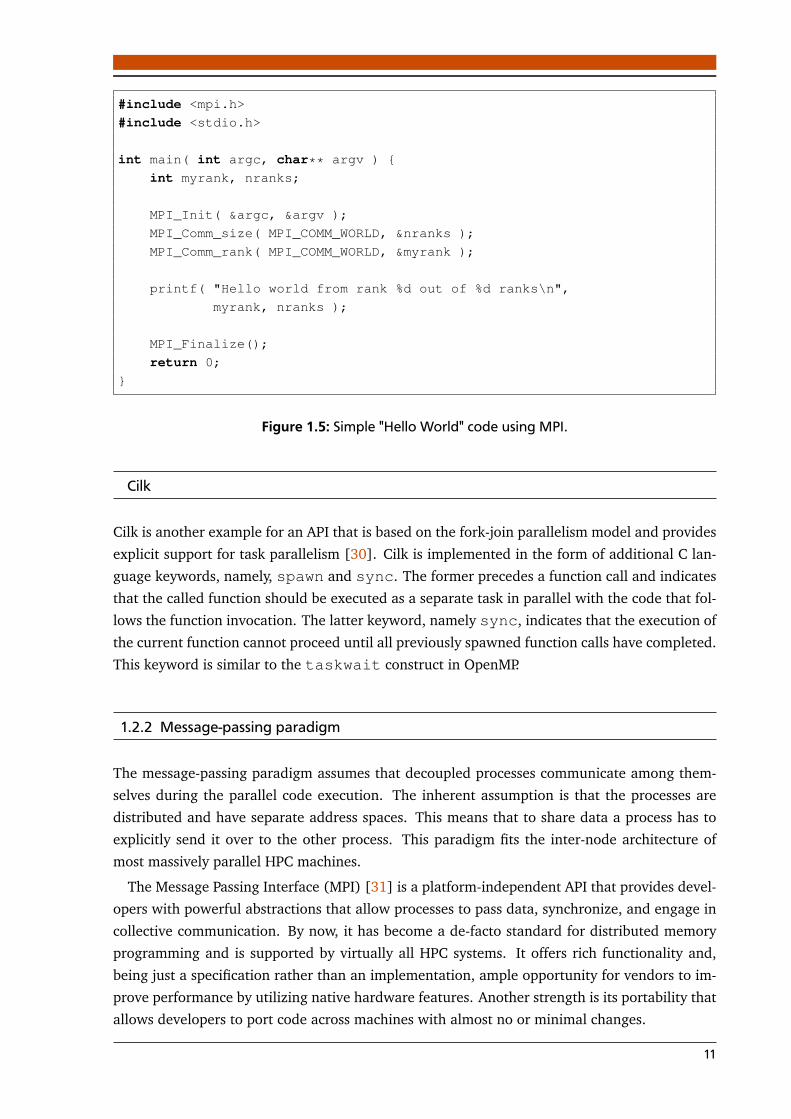
Cilk
Cilk is another example for an API that is based on the fork-join parallelism model and provides
explicit support for task parallelism [30]. Cilk is implemented in the form of additional C lan-
guage keywords, namely, spawn and sync. The former precedes a function call and indicates
that the called function should be executed as a separate task in parallel with the code that fol-
lows the function invocation. The latter keyword, namely sync, indicates that the execution of
the current function cannot proceed until all previously spawned function calls have completed.
This keyword is similar to the taskwait construct in OpenMP.
1.2.2 Message-passing paradigm
The message-passing paradigm assumes that decoupled processes communicate among them-
selves during the parallel code execution. The inherent assumption is that the processes are
distributed and have separate address spaces. This means that to share data a process has to
explicitly send it over to the other process. This paradigm fits the inter-node architecture of
most massively parallel HPC machines.
The Message Passing Interface (MPI) [31] is a platform-independent API that provides devel-
opers with powerful abstractions that allow processes to pass data, synchronize, and engage in
collective communication. By now, it has become a de-facto standard for distributed memory
programming and is supported by virtually all HPC systems. It offers rich functionality and,
being just a specification rather than an implementation, ample opportunity for vendors to im-
prove performance by utilizing native hardware features. Another strength is its portability that
allows developers to port code across machines with almost no or minimal changes.
11

The abstraction presented to developers is of P processes with separate address spaces that
run simultaneously and communicate with each other. The MPI environment spawns the same
executable on different nodes and possibly multiple instances on the same node. Though in
most cases the processes will execute the same program (with different data), a single process
or a group of processes can branch into an entirely different code. In other words, MPI supports
both the single program, multiple data (SPMD) execution model and the multiple programs,multiple data streams (MPMD) execution model. Figure 1.5 presents a simple "Hello World"
code using MPI. In most cases, the initialization routine MPI_Init should be the first MPI
routine a process calls. After calling it, each process determines the total number of processes
in a communicator and its rank (i.e., a unique sequence) among these processes by calling
MPI_Comm_size and MPI_Comm_rank, respectively. A communicator is a group of MPI
processes with a communication context, such that a message sent in one context cannot be
received in another context. Ignoring spawned processes and inter-communicators, the constant
MPI_COMM_WORLD specifies the default communicator that includes all the MPI processes. In
the end, the finalization routine MPI_Finalize allows MPI to cleanup data structures and
deactivate itself. Except for some very specific cases, it is assumed no MPI communication
routines are called beyond this point.
The basic features of MPI are point-to-point communication routines, collective communica-
tion operations, and communicator-related and topology-related functions. Specifically, point-
to-point communication means that one process sends a message to another process, while
collective communication means that all the processes in the communicator are involved in the
operation. Topology-related functions focus on topology, which is an attribute of a communica-
tor and provides a convenient naming mechanism for processes. It can also assist in mapping
the processes onto hardware. As the MPI standard evolved, more advanced features, such as
one-sided communication, neighborhood communication, and I/O, were added to it [32]. Our
discussion in subsections below is motivated by the MPI case study in Chapter 3, which focuses
just on a small selection of collective operations, communicator-related functions, and topology-
related functions. We start with a short overview of point-to-point communication routines that
will allow us to explain the semantics of collective operations more easily.
Point-to-point communication
Point-to-point communication in MPI is performed by one process sending a message to another
process and by the other process posting a distinct receive to retrieve the message being sent.
The standard defines a number of variations of send/receive functions. The most simple ones
are MPI_Send and MPI_Recv, which are blocking send and receive operations, respectively.
It means the send call does not return until either the message was buffered or has successfully
left the node, that is, the matching receive call has been posted. The same is true for the
blocking receive call—it does not return until it retrieves the message. Processes can send
arrays of predefined MPI data types, such as MPI_INT or MPI_DOUBLE, or define new data
types. MPI performs the necessary type matching and conversion, such as converting from
little-endian to big-endian.
12

The non-blocking variant of send and receive operations allows codes to overlap communica-
tion and computation. The function MPI_Isend has the same purpose as MPI_Send, but it is
not a blocking call and the process can continue running. As an output, it provides an instance
of MPI_Request, which is a request handle and can be used later to query the status of the
communication or wait for its completion. The matching MPI_Irecv function also returns
immediately. It indicates that the system may start writing data into the receive buffer. The
process can call MPI_Wait, which is a blocking call, and pass an instance of MPI_Request
to wait for the non-blocking operation to complete. In a typical scenario, the process will call
MPI_Wait once it has completed some intermediate computation and now needs to wait for
the completion of the communication part before continuing. Alternatively, the process can use
MPI_Test, which is a non-blocking call, just to check whether the communication operation
has been already completed or still continues. Although these two variants of send and receive
are just a small glimpse into a wide range of other variants, they provide a good overview of
point-to-point communication.
Collective communication
Contrary to having one sender and one receiver in the point-to-point communication, collective
communication is defined as a communication that involves all of the processes in a communi-
cator. It means that all the processes have to call the collective function for it to work properly.
If one process is delayed and arrives at the call later than the others, the completion of the call
will be delayed. For simplicity, we cover here only the blocking variant of collective operations.
We can categorize most of the collective operations into four groups: (i) all-to-all—all pro-
cesses contribute to the result and receive the result; (ii) all-to-one—all processes contribute to
the result and only one process receives the result; (iii) one-to-all—one process contributes to
the result and all the processes receive the result; and (iv) collective operations that implement
parallel prefix-sum, that is various variations of MPI_Scan. Some of the operations have a
single originating or receiving process. In these cases, it is called the root process and can be
any of the participating processes.
Below is a short overview of the most common collective operations that are used in the MPI
case study in Chapter 3:
• MPI_Barrier—a special case of an all-to-all operation to synchronize the processes.
No data is sent between the processes, but every process participates in this operation.
The call blocks the caller until all other processes have called it. In other words, it returns
at any process only after all other processes have entered the call.
• MPI_Bcast—a one-to-all operation that broadcasts a message from the root process to
all other processes, itself included.
• MPI_Reduce—an all-to-one operation which combines the input buffers (i.e., messages)
of each process using a predefined operation, such as maximum or sum, and places the
result in the root. Developers can define additional reduction operations of their own, but
they have to be associative.
13

• MPI_Allreduce—an all-to-all operation, which is very similar to MPI_Reduce, but
all the processes receive the result and not just the root. It is equivalent to MPI_Reduce,
followed immediately by MPI_Bcast with the same root.
• MPI_Gather—an all-to-one operation in which each process (including the root) sends
a message to the root, which receives all the messages and stores them in rank order. It is
equivalent to each process calling MPI_Send and the root process calling MPI_Recv Ptimes (assuming P is the number of MPI processes in the communicator).
• MPI_Allgather—an all-to-all operation, which is very similar to MPI_Gather, but
all the processes receive the messages instead of just the root. It is equivalent to
MPI_Gather followed immediately by MPI_Bcast with the same root.
• MPI_Alltoall—an all-to-all operation, which can be viewed as an extension of
MPI_Allgather, in which each process sends out distinct data to all the other pro-
cesses. It is equivalent to each process calling MPI_Send P times, each time with a
different rank, and then calling MPI_Recv P times.
Communicator-related functions
Communicator-related functions are functions for managing communicators. Some of these
functions, such as functions to create, duplicate, and free communicators are collective oper-
ations and require all the MPI processes in the communicator to participate. Below is a short
overview of the functions that are used in the MPI case study in Chapter 3:
• MPI_Comm_create—creates a new communicator from a given group of processes.
The new group has to be a subset of the group of the current communicator. This function
can be used, for example, if we need to run a collective operation that involves just some
smaller subset of the processes.
• MPI_Comm_dup—duplicates an existing communicator, such that the new communica-
tor has the same processes, topology, and attributes, but a different context. The primary
goal of this function is to be used by 3rd party libraries (e.g., mathematical libraries) to
create a separate context for communication such that the library does not interfere with
the communication outside.
• MPI_Comm_free—frees the communicator, but before deallocating the communicator
object makes sure that any pending operations that use this communicator are completed
normally.
Topology-related functions
A topology is an attribute of a communicator and allows processes to be arranged in a spe-
cific pattern. By default, it is a linear ranking such that each process in a communicator has a
14

Observation Analysis Optimization
Simulation
Performance
modeling
Figure 1.6: Performance engineering cycle of applications in HPC.
rank number in a sequence between 0 to P − 1 (assuming P is the number of MPI processes
in the communicator). In many codes, however, this sequence does not adequately reflect the
logical communication pattern between the processes, which is usually determined by the prob-
lem geometry, domain decomposition, and the numerical algorithm in use. Topology-related
functions allow developers to construct new communicators that arrange the processes in spe-
cialized topologies, such as 2D or 3D grids. One prominent example, which constructs Cartesian
topologies of arbitrary dimensions, is the function MPI_Cart_create. Using the functions
MPI_Cart_coords and MPI_Cart_rank developers can translate the Cartesian coordi-
nates of a process in a Cartesian communicator to its rank in that communicator and vice
versa.
1.3 Performance Analysis and Engineering
The previous sections provided a short overview of typical HPC systems as well as discussed a
number of parallel programming paradigms programmers use to harness the computing power
of these systems. Parallel programming entails non-trivial challenges and, remembering the old
saying that “premature optimization is the root of all evil” [33], programmers focus initially on
making their parallel programs produce correct results. However, merely achieving correct re-
sults is a necessary condition to begin realizing the potential of HPC systems, but it is definitely
not a sufficient one. The goal is to maximize the amount of “completed science per cost and
time” [34]. Since HPC systems are limited in lifetime and expensive, we have to optimize the
applications as well as system architecture, scheduling, and topology mapping. In this work,
however, we specifically focus on applications and the optimization goals in this case are execu-
tion time, scalability, efficiency, energy consumption, memory usage, and so on. For example,
faster execution means more “science per time”, better scalability translates into higher-fidelity
simulations, and better efficiency means that less resources are wasted.
The process of systematic performance analysis and tuning of applications is called perfor-mance engineering [34, 35]. Figure 1.6 presents a diagram of this process. It consists of three
steps (plus 2 optional steps) arranged in a cycle that might be repeated a number of times until
our performance goals are achieved. We start with initial observations that provide us with per-
formance data. This step usually involves performing measurements by means of profiling and
15

benchmarking. We then continue to the analysis step in which we study the performance data
along with our code in more depth using various tools and visualization techniques. We might
also perform more measurements to gather specific counter and metrics data. The goal in this
step is to gain an initial understanding of potential bottlenecks and identify optimization op-
portunities. One particular example is identifying hot spots, specific places in the code in which
the application spends considerable amount of time and thus are good candidates for optimiza-
tion. Following the analysis step are two optional steps, namely, simulation and performance
modeling, respectively. Simulation is a form of rudimentary modeling as it allows us to simu-
late isolated aspects of our application (e.g., specific functions or communication patterns) on a
hypothetical hardware, thereby providing us with accurate predictions. It appears as a separate
step in the figure to emphasize that it is different from performance modeling since it does not
give us an analytical expression and might be too slow and expensive for analyzing behavior
at larger scale [34]. The performance modeling step, which includes analytical modeling and
empirical modeling, has a number of advantages that will be discussed below. Finally, we reach
the step of code optimization, in which we apply suitable optimization strategies that might
involve, for example, efficient cache use and computation-communication overlap. In general,
optimization is a separate, very rich field of research and there is no single solution that fits
all the HPC applications. In most of the cases, we would continue to another iteration of the
engineering cycle to verify the optimized sections of the code and to identify new bottlenecks.
In the subsections below, we provide a brief overview of the observation, analysis, and per-
formance modeling steps. The goal is to construct the necessary context for this dissertation
rather than provide a comprehensive overview. For this reason, we do not cover the simulation
and optimization steps in detail.
1.3.1 Observation
In the observation step, we collect the performance data of our code. The simplest approach is
just benchmarking, that is running the code repeatedly (i.e., repetitions increase our confidence
in the results), measuring the execution time, and then collating the results. In most cases this
approach is too coarse grained and will not expose any hot spots in the code. We have to obtain
more fine grained performance data by means of either instrumentation or sampling.
Instrumentation. Instrumentation is a technique in which performance measurement calls
are inserted into the original code or are placed as hooks that intercept API calls. During the
code execution these calls are invoked and allow the performance measurement tool to record
various performance data such as timestamps, memory usage, and so on. Well known tools,
such as Score-P [36], intercept MPI calls and insert calls before and after function invocations
in the code. As a result, Score-P is able to construct a call tree with performance information
(e.g., execution time, number of visits, bytes sent and received) for each node (including MPI
functions). In Score-P, such a call tree is called performance profile as it summarizes the perfor-
mance of the entire execution and can be produced without keeping all the recorded data. In
tracing, on the other hand, performance data contains individual events recorded throughout
16

either the entire execution or parts of the execution. This data is called a trace and is kept for
later, post-mortem analysis.
Sampling. One problem with instrumentation is performance perturbation since calling func-
tions to record performance data introduces overheads, such as longer execution times, or ex-
acerbates existing issues, such as late arrivals of processes to MPI calls. As a solution, sampling
allows performance tools to interrupt the execution of the code at periodic intervals and record
relevant performance data (e.g., function visits). Some of the sampling tools unwind the stack
to retrieve call-path information and construct the call tree [37, 38]. The execution time of a
function is estimated by multiplying the percentage of visits by the total execution time. The
interrupt interval, or sampling frequency, should be chosen carefully, since a shorter interval
might cause significant perturbation, while a longer one might give us less accurate perfor-
mance data. Since no instrumentation is involved, sampling can be used without recompiling
the code.
1.3.2 Analysis
In the analysis step, we analyze the performance data collected earlier. In most cases, the goal
is to reveal potential bottlenecks or identify hot spots for optimization. Good analysis tools
facilitate the identification of hot spots by allowing users to easily navigate and explore the
collected data. For example, Figure 1.7 shows two screenshots from well known performance
analysis tools for HPC applications, namely, Scalasca [39] and Vampir [40]. Scalasca collects
performance profiles using Score-P and uses the CUBE tool [41] for their visualization and
exploration. Figure 1.7a shows a snapshot of the CUBE graphical user interface that displays
performance data in three panes. The panes correspond to different dimensions of performance
data, namely, metric, call-tree, and system. In the left pane, users select a metric such as
execution time, transferred bytes, and so on. The middle pane shows the call tree that can be
expanded or collapsed. Values for the selected metric are shown next to the tree nodes. The
right pane is reserved for plugins. The default plugin is the system dimension, which presents
a tree of nodes, processes, and threads. Vampir and other tools such as Extrae [42] are based
on traces and visualize them along the time axis. Figure 1.7b, for example, shows a snapshot of
the Vampir tool. The main pane in the upper left side presents the traces—one for each process.
The choice of colors for different parts of the trace provides a clear delineation between the
communication phase (red color) and the computation phase (blue color). Such information is
instrumental for identifying imbalances in the execution of the code. The lower left pane shows
the trace data in the form of a plot for the floating point operations counter in process 0. Note
that the timeline and the counter plot are aligned so that it is clear that the drop in the floating
point rate in process 0 is due to communication.
Mature performance analysis tools of HPC applications, such as Scalasca and Vampir in Fig-
ure 1.7, are the first choice for our efforts to understand and optimize our code. However, these
tools are also limited in scope since they do not show us how close we are to the optimum per-
formance or whether issues which seem negligible at current scale will become major problems
at extreme scale.
17

(a) Scalasca
(b) Vampir
Figure 1.7: Examples of common performance analysis tools.
18

1.3.3 Performance modeling
Performance modeling expresses different aspects of application performance with analytical
expressions. A model of execution time as a function of the number of processes, for example,
shows us how the applications scales by predicting execution time at a higher scale. A model
of execution time as a function of the input gives us an analytical expression of the algorithm
complexity (e.g., T (n) = 2.2n3 for simple matrix-matrix multiplication [34]). These models can
be analytical models, that is constructed manually by careful analysis of the code, or empiricalmodels, that is models driven entirely by measurements of the code performance. Another
class of models are requirements models, which express requirements, such as the number of
floating point operations needed to solve the problem, independently of the architecture. For
example, the number of floating point operations required to solve the (naïve) n × n matrix-
matrix multiplication problem is f (n) = 2n3 since we have three levels of nested n-iterations
loops, and one multiplication and one addition in the inner-most loop.
Usually the performance engineering cycle in Figure 1.6 is repeated until we reach a perfor-
mance level that is sufficient for our needs. The question, however, is how do we know we are
close enough to the optimum performance? First, to estimate the optimum we can combine
requirements models with system characteristics such as peak floating point performance. This
provide us with an understanding of the full performance potential. Second, a better goal for
performance tuning would be to reach a performance level that is within some fraction of the
optimum. This is where the advantage of analytical and empirical models could be used to the
fullest. Not only can they give us insight into how close we are to the optimum, but they also
allow us to see whether further optimization opportunities are still available.
Although analytical modeling is very useful for better performance engineering, it is not easy
to construct models for different parts of an application. It is a very laborious process that
requires time and expert knowledge of the code. In Chapter 2, we provide an overview of the
state-of-the-art of empirical performance modeling. Specifically, we describe a technique for
automated construction of empirical models. This technique generates empirical models for
each function (or code section) accurately and quickly [43]. In this way, performance modeling
can be applied systematically to tune the performance of applications, as well as optimize the
system architecture. The latter aspect relates directly to the process of co-designing future
systems.
1.4 Motivation and Scope
The motivation in this dissertation is to engineer HPC applications for better scalability. In the
beginning of the chapter, we discussed future extreme-scale HPC systems and the increased
multi-level parallelism they will provide. The challenge is to exploit this parallelism in an
effective way. Traditionally, developers optimize their codes by following the performance en-
gineering workflow described in the previous section. This approach, however, is not enough,
since the sheer scale and the levels of parallelism in upcoming systems will make it difficult to
test the code on the full scale of the system.
19

Scalability can be defined as the measure of the application and system capacity to increase
the speedup (i.e., the ratio of sequential execution time to the parallel execution time) in propor-
tion to the number of processes or processing elements (i.e., either cores or nodes) [25, 35, 44].
Note that in our discussion we use the notion of the number of processes and the number of
processing elements interchangeably since the former is increased in a constant proportion to
the latter. Since parallel efficiency is defined as the ratio of the speedup to the number of pro-
cesses, the scalability definition means that the goal is to maintain a constant efficiency as the
number of processes increases. We can identify three types of scalability (p is the number of
processes and n is the input size):
• Strong scalability—in this scenario, p increases and n remains constant, and the goal of
maintaining constant efficiency translates into minimizing the parallel execution time.
• Weak scalability—in this case, n= C p, where C is constant. In other words, n is increased
in a constant proportion to p, and the input size per process remains constant. The goal
is to make sure the execution time stays constant or increases very slowly.
• General scalability—we denote the relation between n and p as a function n = fE(p),which changes according to the efficiency E we want to keep constant. The goal, in this
case, is to make sure the function fE is grows reasonably slowly. Otherwise, the input size
will become prohibitively big for higher number of processes.
In the next section, we describe our contributions that tackle the challenge of exploiting in-
creasing parallelism, thereby ensuring applications scale well on extreme-scale systems. We
adopt a performance-centric engineering methodology that addresses the above scalability sce-
narios throughout the entire software development process, which typically starts from the
analysis phase, continues to design and implementation, and finishes with testing.
1.5 Dissertation Contributions
In this dissertation, we develop two approaches in which we use empirical models, produced
with automated techniques, to gain insights into the code behavior at scale. These approaches
allow for better scalability engineering and can be used not only in the traditional software
development cycle, but also in other related fields, such as algorithm engineering [45].
The first contribution is a new software engineering approach for extreme-scale systems,
which essentially combines empirical performance models produced automatically with the test
phase in the software development cycle. Specifically, we develop a framework that validates
asymptotic scalability expectations of programs against their actual behavior. The most impor-
tant applications of this method, which is especially well suited for libraries encapsulating well-
studied algorithms, include initial validation, regression testing, and benchmarking to compare
implementation and platform alternatives. The expectations do not need to be precise analyt-
ical expressions involving measurable metrics. The user needs only to provide the asymptotic
growth rate of the function/metric pair in question, making this a simple but effective solu-
tion for future extreme-scale library development. The framework automates large parts of the
20

workflow, thus allowing it to be continuously applied throughout the development cycle. The
first, and perhaps the most important, case study for evaluating the framework is MPI collective
operations. Using the framework, we identify a number of scalability issues, including unex-
pected behavior of key collective operations and excessive memory consumption by MPI on one
of the test machines. This approach enables MPI developers to spot scalability bottlenecks early
on, before commencing full-scale tests on the target supercomputer. We also show an evaluation
of the framework on a data-mining code and various OpenMP constructs.
The second contribution focuses on practical isoefficiency analysis of task-based programs.
Isoefficiency is a concept borrowed from theoretical algorithm analysis, it binds efficiency, pro-
cessing elements count, and the input size in one analytical expression, thereby allowing the
latter two to be adjusted according to given realistic efficiency objectives. In other words, an
isoefficiency function shows us by which factor the input size (i.e., the problem size) has to
increase in relation to the number of processes in order to maintain a constant efficiency. Ac-
cording to our definition of scalability in the previous section, maintaining constant efficiency
means that our application is scalable. However, it does not mean that this scalability is sus-
tainable. It is clear that a quickly growing isoefficiency function will quickly require us to have
prohibitive input sizes and will result in the application taking too much time to finish execu-
tion. In this contribution, we show how to determine the realistic isoefficiency function for a
target efficiency empirically. A realistic isoefficiency function allows users to evaluate whether
the application is sustainably scalable and make informed decisions as to how big the input size
should be in order to use all of the available cores efficiently.
One factor which influences the isoefficiency function is resource contention that results from
limited resources, such as cache and memory controllers. To understand the effects of re-
source contention on efficiency we devise a method to produce a contention-free replay of a
task-based program and determine the isoefficiency function of this replay. By comparing the
isoefficiency functions of the program itself and its contention-free replay, one can attribute
poor scaling either to excessive resource contention overhead or structural conflicts related to
task dependencies or scheduling. As part of this contribution, we also used empirical perfor-
mance modeling to model how the depth and the average parallelism of a task-based program
change as the input increases. These models allow users to identify scalability bugs in their pro-
grams. Average parallelism that scales poorly compared to the depth indicates that the program
would not run optimally for larger inputs. The approach was evaluated on two benchmark
suites and the obtained results demonstrate that it can help users, application developers, and
hardware designers address a number of important issues, related to both application analysis,
deployment, and co-design.
1.6 Dissertation Structure
The structure of this dissertation is as follows. We begin with a discussion of the state-of-
the-art in automated empirical modeling of performance in Chapter 2. This chapter describes
the modeling workflow, covers the Extra-P tool, which is used extensively in this work, and
finishes with an overview of the approach to model functions with more than one parameter.
21

Following Chapter 2, we present each contribution of this dissertation in a separate chapter.
Chapter 3 presents our scalability validation framework including the case studies that were
used to evaluate it. Chapter 4 describes the Task Dependency Graph (TDG) abstraction and
presents the techniques for constructing, analyzing, and replaying TDGs. This chapter lays the
foundation for Chapter 5, which discusses our second contribution, namely the technique for
practical isoefficiency analysis. We continue with Chapter 6 that covers studies related to each
one of the contributions. Finally, Chapter 7 finishes with conclusions and an outlook of future
research.
22

2 Empirical Performance ModelingThis chapter focuses on the state-of-the-art in automated empirical performance modeling,
specifically, the results of Calotoiu et al. [43, 46], and provides the necessary background
needed to understand the techniques in Chapters 3 and 5. Most of the work was conducted
as part of the Catwalk project [47, 48] under the auspices of the DFG Priority Programme 1648
Software for Exascale Computing (SPPEXA).
2.1 Overview
As was briefly discussed in Section 1.3.3, analytical performance modeling expresses different
aspects of application performance with analytical expressions. It is a powerful technique in
performance engineering as it allows developers to get a preliminary feedback on the design
of their applications. They can, therefore, understand how close the performance is to the
optimum or adapt the design to the requirements of larger problem and machine sizes.
Analytical performance modeling was successfully used in a number of previous stud-
ies [49, 50, 51] to model the performance of HPC applications. The process of constructing
the models, however, is very laborious and requires time and expert knowledge about the code.
First, an initial model is suggested following an in-depth analysis of the algorithms, and then
experimental data is gathered to find the exact coefficients in the model and to verify its correct-
ness. It is easy to see that this a trial-and-error approach that requires the person performing
the analysis to be a domain expert or to work closely with one. If the first guess of the model
is incorrect, a different model has to be suggested and verified against the experimental data.
Moreover, the process has to be repeated for each part of the code we want to model. The
technique for empirical performance modeling we discuss in this chapter is mostly automated.
It constructs empirical models, as well as requirements models, for each function (or code sec-
tion) accurately and quickly. This means no domain expert is required and all the code can be
covered in the analysis. This technique was first studied by Calotoiu et al. [43] in the context of
identifying scalability bugs. A scalability bug is a part of the program in which scaling behavior
is unintentionally not good. Figure 2.1 gives an overview of the different steps necessary to find
these bugs. This workflow can be used not only to search for scalability bugs, but also produce
performance models that can improve our performance engineering efforts. In other words,
these models can predict future performance and provide us with insights into the application
behavior, such as the compute time needed to solve a larger problem.
The technique for automated empirical modeling has a number of limitations. It is sensitive
to noise in the measurements and to behavior that changes unexpectedly, for example, when
a function switches its algorithm for some specific input or number of processes. Besides, as
discussed below, this technique uses a specific form for the models and cannot model accurately
23

Performance
profilesPerformance
profilesPerformance
profiles
Performance
measurements
Statistical
quality control
Model
generation
Model
refinement
Scaling
modelsScaling
modelsScaling
models
Accuracy
saturated?
Performance
extrapolationRanking
of kernelsRanking
of kernelsRanking
of kernels
Kernel
refinement
Comparison
with user
expectations
Yes
No
Figure 2.1: Workflow of scalability-bug detection proposed by Calotoiu et al. [43] that can begeneralized to empirical performance modeling in general. Dashed arrows indicate optionalpaths taken after user decisions.
code that behaves in a very unusual way. In such cases, the traditional analytical modeling has
an advantage, since it allows us to tailor very specific models for such codes.
The workflow in Figure 2.1 begins with a set of performance measurements on different
processor counts {p1, . . . , pmax}. The measurements produce performance profiles, similar to
profiles discussed in Section 1.3.1. Computing systems in general, and HPC systems in par-
ticular, are prone to jitter (i.e., noise). This means that to ensure the measurements produce
statistically sound results, they have to be repeated a number of times. Even if the OS itself is
optimized to be as noiseless as possible, such as the CNK on the Blue Gene/Q machine [52],
noise and unexpected interference in the network are still possible. The amount of measure-
ment repetitions depends on the variation of the results. Once this is accomplished, Calotoiu et
al. apply regression to obtain a coarse performance model for every possible program region,
which is a node in a call-path tree. These regions are called kernels since they define the code
granularity at which the models are generated. The granularity of the kernels can be further
increased by using a more fine-grained instrumentation, such as the manual instrumentation in
Extra-P [36]. The initial performance models undergo an iterative refinement process until the
model quality reaches a saturation point.
The next sections discuss the model generation processes in more detail and present the
Extra-P tool, which embodies the workflow for empirical performance modeling presented in
Figure 2.1. In Section 2.5, we explain the multi-parameter modeling approach which is based
on the same modeling workflow, but produces models with two or more parameters.
2.2 Performance Model Normal Form
A key concept of the performance modeling approach is the performance model normal form(PMNF), defined in Equation 2.1. A PMNF model reflects how a performance metric, such as
execution time or a performance counter, changes as a function of a single parameter p. The
idea behind PMNF is the observation that performance models are usually composed of a finite
number n of predefined terms, involving powers and logarithms of p. The PMNF limits the
24

scope of functions we can represent with it. However, it works in most scenarios encountered
in practice, as a consequence of how most computer algorithms are designed [43].
f (p) =n∑
k=1
ck · pik · log jk2 (p) (2.1)
The successful use of PMNF in previous studies [43, 53, 54, 55] indicates that neither the
number of terms n nor the sets I , J ⊂ Q, from which the exponents ik and jk are chosen, have
to be large to achieve a good fit. We have to select reasonable values for n, I , and J , and then
try the different models in the resulting space one by one. For example, a default choice often
used is given in Equation 2.2 [54, 56]. Although such a default configuration can be sufficient
in many cases, it is not a good fit for some applications. In these cases, the search space has to
be tuned manually, with the help of domain experts and application developers, by modifying Iand J . We call model hypothesis a possible assignment of ik and jk in a PMNF expression.
n= 2
I = {04
,14
,24
, . . . ,124}
J = {0, 1,2}(2.2)
As an alternative to the number of processes p, other model parameters such as the size of
the input problem (or other algorithmic parameters) can be used.
2.3 Model Generation
In this section, we look closely at the model generation process. As discussed earlier, the input
of the performance modeling workflow, and specifically, the model generator, is a set of perfor-
mance profiles, representing runs with one changing parameter. The profiles can be obtained
using existing performance measurement tools such as Score-P [36], which collects several
performance metrics, including execution time, and various hardware and software counters,
broken down by call path and process. However, we also have the flexibility to measure per-
formance manually and provide the model generator with textual input data (see Section 2.4).
Based on performance profiles, one model is produced for each combination of target metric
and call path, enabling a fine-grained scalability analysis of complex applications. Piece-wise
defined functions and irregularities in the code that cannot be modeled by PMNF will lead to
sub-optimal results. This also implies that the model generator cannot automatically determine
at which scale particular behaviors start manifesting themselves.
Experience from past studies [43, 53, 54, 55] indicates that as few as five different measure-
ments for one parameter are enough for a successful model generation. If noise and jitter affect
the measurements, experiments for each value of the input parameter should be repeated until
the data provides reasonably tight confidence intervals. As a rule of thumb, confidence intervals
at the 95% or 99% confidence level should be no larger than 5% of the sample mean. This en-
sures the results of the modeling are statistical significant. Since we need to run experiments for
25

at least five different values of the input parameter, as well as repeat each experiment several
times, the computational cost of gathering enough data for modeling can quickly add up and
become an issue. It is necessary, therefore, to design the experiments carefully and keep the
execution time of each experiment in check by selecting appropriate values for the application
parameters. In a weak scalability study, for example, we do not need to run the experiments at
very large scales unless we suspect that the application would behave qualitatively different at
these scales. A qualitative difference in this context could be the result of changing an algorithm
for part of the application past a certain processor count, which is done, for example, in some
MPI collective operations [54].
Once the profiles are available, the model generator constructs the models in an iterative pro-
cess, which is illustrated in Figure 2.2. In each step, a number of model hypotheses of a certain
size (i.e., number of terms) are instantiated according to the PMNF defined in Equation 2.1.
The hypothesis with the best fit across all candidates is selected through cross-validation. The
process starts with a one-term hypothesis, but with each new iteration one additional term is
added to the hypothesis size. The iterations continue until the process arrives at the configurable
maximum model size or begins to over-fit the data. The adjusted coefficient of determination
R2 [57], a standard statistical factor used in regression analysis, indicates which share of the
variation in the data is explained by the model function. Its values are between 0 and 1, and
values closer to 1 indicate a better quality of fit. For further details of the model generation
process including references to the statistical methods employed we refer the reader to Calotoiu
et al. [43].
2.3.1 Automated refinement algorithm
In order to instantiate candidate hypotheses, the process illustrated in Figure 2.2 relies on
values and ranges the user provides for n and I , J ⊂ Q. One possible example is presented in
Equation 2.2. Essentially, this defines a search space in which the model generator searches for
the best-fitting model. A major disadvantage with this approach is that the user does not know
initially whether the search space is big enough, and after getting the first models, the values
of n and I , J ⊂ Q might need to be updated to get models that can better fit the data. Not only
does this process require more expertise from the user, but it is also time consuming.
As a solution, Reisert et al. [56] proposed an automated refinement algorithm for model con-
struction. It configures the search space on demand and by automatically refining the model it
increases the accuracy until no meaningful improvement can be made. The proposed approach
limits the PMNF to only two terms (n = 2) with the first term being a constant term and uses
a special metric, called symmetric mean absolute percentage error (SMAPE), to better evaluate
one model against the other in terms of their fit. With this new automated refinement approach
users no longer need to specify the ranges of I , J ⊂ Q or the value for n. However, one ma-
jor limitation of this approach is that it lacks support for negative exponents. This means that
it cannot model execution times that represent strong scaling directly. To overcome this lim-
itation and model strong scaling behavior, execution times have to multiplied by the number
26

Input data
Hypothesis generation
Maximum hypothesis size ω
Hypothesis evaluation
via cross-validation
Computation of R2ω
for best hypothesis
R2ω−1 ≥ R2
ω ∨ ω=ωmax
Performance
model
ω= 1, R20 = −∞
Yes
No; ω++
Figure 2.2: Iterative model construction process (taken from Calotoiu et al. [46]).
of processes. This gives us a so called work time that, in ideal strong scaling, should remain
constant.
Since the automated refinement algorithm was developed relatively recently, most of the
studies that used empirical modeling [43, 53, 54, 55, 58], including the next chapters in this
dissertation, relied on the original approach, which is illustrated in Figure 2.2. However, we
mention the new algorithm here to provide a complete picture of the state-of-the-art in auto-
mated empirical performance modeling.
2.3.2 Segmented regression
Another fairly recent development is the work by Kashif et al. [59] that added the capability
of segmented regression to the modeling workflow. The problem this study aims to solve is
related to the cases in which a kernel substantially changes its behavior for some range of the
input parameter. A substantial change means that a different model is needed to explain the
new behavior. One example is when an MPI collective operation changes its algorithm once the
number of processes or the message size passes a certain threshold. This results in a series of
measurements that cannot fit accurately just one model, and so we need to find an inflection
point, or possibly a number of inflection points, and fit a different model for each segment
between these points. The segmented regression study implemented an experimental model
generation algorithm that tries different potential inflection points and checks whether the two
new models give us a better fit. Naturally, this approach requires using more values for the
input parameter, since each segment is smaller than the whole range of values we have. This
study produced encouraging results and since we often do not expect two different behaviors in
our results this is an important capability to catch these cases and still produce accurate models.
27

Table 2.1: Examples of empirical models produced in different studies. The left column listsapplications with kernels or libraries with functions or constructs. The right columns shows thecorresponding performance models of execution time.
Application (or library) / Kernel Model (execution time)
Sweep3D / sweep (MPI_Recv) [43] 4.03 · pp
HOMME / vlaplace_sphere_wk [43] 24.44+ 2.26 · 10−7 · p2
UG4 / CG [55] 0.23+ 0.31 · pp
UG4 / GMG [55] 0.22+ 6 · 10−4 · log2 p
OpenMP (GNU) / parallel [53] 3.98 · 10−7 · p1.25
OpenMP (Intel) / barrier [53] 9.76 · 10−6 · p0.25
MPI (Juqueen) / MPI_Bcast [54] 4.91+ 0.11 · log p
MPI (Piz Daint) / MPI_Gather [54] 20.55+ 0.11 · p
2.3.3 Application examples
To better understand the output of the model generation process and how models based on
PMNF look like in practice, Table 2.1 shows concrete examples from previous studies. All of
the models are based on the ranges for I , J ⊂ Q specified in Equation 2.2. In almost all of
the studies, models with only two terms were enough to capture the main behavior of the
kernel or construct. In fact, one should be careful with using more terms, since it can result
in over-fitted models that capture the noise in the data rather than the actual behavior of the
code. The first two examples, namely, Sweep3D and HOMME, are taken from the original
scalability-bugs study by Calotoiu et al. [43]. The HOMME model clearly shows a scalability
bottleneck in the evaluated kernel. The UG4 application was evaluated by Vogel et al. [55] and
some of the kernels were found to have scalability bottlenecks as well. The next two examples,
namely, parallel and barrier, show models for OpenMP constructs. This work evaluated different
OpenMP runtimes by producing empirical models for the main OpenMP constructs. Since this
example is an important use case for our first contribution in this dissertation, we discuss it in
more detail in Chapter 3. The final two examples show models of MPI collective operations.
This is our leading case study of the first contribution of this dissertation (see Section 1.5),
namely the scalability validation framework, and it is discussed in greater detail in Chapter 3 as
well.
2.4 Extra-P
The Extra-P tool [60] embodies the workflow for empirical performance modeling presented
in Figure 2.1. It is designed to be a general-purpose tool to be used with various kinds of
applications and use cases. It provides both textual and graphical user interfaces, and produces
results that can be explored interactively. Extra-P works either with Cube4 [41, 61] input files
or plain textual files. As described earlier, Score-P is one possible performance profiling tool
that we can use since its output is in Cube4 format. However, there also is a simple generic
28

POINTS 8 16 32 64 128
EXPERIMENT Time/MPI_Recv
DATA 0.283169 0.285326 0.289267
DATA 0.458113 0.473634 0.449258
DATA 0.608647 0.598367 0.620311
DATA 0.904977 0.881244 0.893256
DATA 1.20038 1.19564 1.21402
Figure 2.3: Example of Extra-P’s plaintext format for performance experiments.
Plot of
the model
Selected
kernel(s)
Call tree
exploration
Figure 2.4: The graphical user interface of Extra-P based on PyQt.
text-based format, such that any other measurement tool and workflow can be used as well by
converting its output into the text-based format.
Figure 2.3 shows an example of the measurement results, specifically, the results of profil-
ing a single call path, in Extra-P’s textual format. The first line, starting with the keyword
POINTS, introduces the values of the model parameter (i.e., p in the PMNF), which in this
case is the number of processes. It means that the application has been profiled running on 8,
16, 32, 64, and 128 processes, which is the minimum number of values needed. The keyword
EXPERIMENT then starts a section for a given performance metric and/or call path, in this case
the Time metric for an MPI_Recv call. A single file can contain any number of such sections.
The following lines that start with the keyword DATA contain the actual measurements for this
experiment in the order of the values defined in the first line. In other words, the first DATA
line corresponds to 8 processes, the second to 16, and so on. The number of measurements in
each DATA line corresponds to the number of repetitions of each experiment. It is three in the
example, but might be much higher.
The current version of Extra-P is implemented in C++ and Python. The core logic is written
in C++ for performance reasons and the graphical user interface (GUI) is written in Python,
using PyQt [62]. The Python code communicates with the C++ core via a defined interface
29
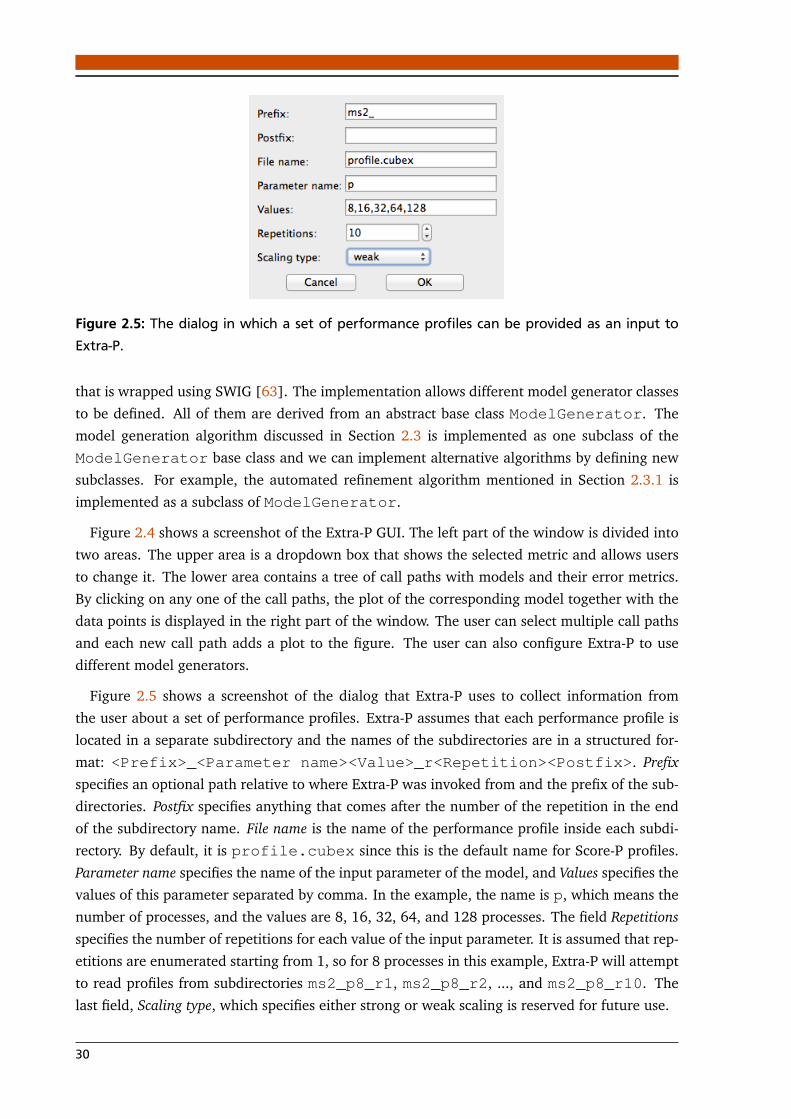
Figure 2.5: The dialog in which a set of performance profiles can be provided as an input toExtra-P.
that is wrapped using SWIG [63]. The implementation allows different model generator classes
to be defined. All of them are derived from an abstract base class ModelGenerator. The
model generation algorithm discussed in Section 2.3 is implemented as one subclass of the
ModelGenerator base class and we can implement alternative algorithms by defining new
subclasses. For example, the automated refinement algorithm mentioned in Section 2.3.1 is
implemented as a subclass of ModelGenerator.
Figure 2.4 shows a screenshot of the Extra-P GUI. The left part of the window is divided into
two areas. The upper area is a dropdown box that shows the selected metric and allows users
to change it. The lower area contains a tree of call paths with models and their error metrics.
By clicking on any one of the call paths, the plot of the corresponding model together with the
data points is displayed in the right part of the window. The user can select multiple call paths
and each new call path adds a plot to the figure. The user can also configure Extra-P to use
different model generators.
Figure 2.5 shows a screenshot of the dialog that Extra-P uses to collect information from
the user about a set of performance profiles. Extra-P assumes that each performance profile is
located in a separate subdirectory and the names of the subdirectories are in a structured for-
mat: <Prefix>_<Parameter name><Value>_r<Repetition><Postfix>. Prefixspecifies an optional path relative to where Extra-P was invoked from and the prefix of the sub-
directories. Postfix specifies anything that comes after the number of the repetition in the end
of the subdirectory name. File name is the name of the performance profile inside each subdi-
rectory. By default, it is profile.cubex since this is the default name for Score-P profiles.
Parameter name specifies the name of the input parameter of the model, and Values specifies the
values of this parameter separated by comma. In the example, the name is p, which means the
number of processes, and the values are 8, 16, 32, 64, and 128 processes. The field Repetitionsspecifies the number of repetitions for each value of the input parameter. It is assumed that rep-
etitions are enumerated starting from 1, so for 8 processes in this example, Extra-P will attempt
to read profiles from subdirectories ms2_p8_r1, ms2_p8_r2, ..., and ms2_p8_r10. The
last field, Scaling type, which specifies either strong or weak scaling is reserved for future use.
30

2.5 Multi-parameter Modeling
Following the success of empirical performance modeling with one-parameter [43, 53, 54, 55],
Calotoiu et al. [46] extended Extra-P to allow users to model the effects of multiple parameters
on different performance metrics.
2.5.1 Extended performance model normal form
The first step was to expand the original performance model normal form to include multiple
parameters, as shown in Equation 2.3.
f (x1, . . . , xm) =n∑
k=1
ck ·m∏
l=1
x ik ll · log jk l
2 (x l) (2.3)
The expanded normal form allows m parameters to be combined in each of the n terms that
are summed up to form the model. Each term now is a product of combinations of monomials
and logarithms. Each component in this product corresponds to a different parameter x l . The
sets I , J ⊂ Q from which the exponents ikland jkl
are chosen, respectively, can be defined as in
the single-parameter case. However, if we look at Equation 2.3 and use the same assumptions
about hypotheses generation as before, we realize that the search space for model hypotheses
is prone to combinatorial explosion. With as few as m = 3 parameters and the default choice
for n and I , J ⊂ Q (e.g., as in Equation 2.2) the model search space would contain more than
107 candidates, making the search for the best fit expensive at best and unfeasible at worst.
2.5.2 Optimization techniques
To deal with the excessive size of the search space, Calotoiu et al. [46] developed two heuristics
to accelerate the search for suitable performance models, making the approach feasible in prac-
tice. The first heuristic speeds up multi-parameter modeling, as it reduces the search space to
include only combinations of the best single parameter models. The second heuristic speeds up
model selection for single parameter models by ranking hypotheses according to their growth
and traversing the search space in a more efficient way (i.e., golden section search), such that
fewer hypotheses have to be evaluated. Combined, the two heuristics reduce a search space of
hundreds of billions of models to just under a thousand.
2.5.3 Application examples
Table 2.2 presents a number of concrete examples of multi-parameter models. They are all in-
stances of the extended PMNF and were generated using the optimization techniques described
above. The first two examples in the figure show the models for the floating point instructions
and the execution time of the LTimes kernel in Kripke, a particle-transport proxy application.
The input parameters are the number of MPI processes p, the number of directions d, and the
31

Table 2.2: Examples of empirical multi-parameter models produced in different studies. The leftcolumn shows the metric and the parameters.
Metric (parameters) Model
Kripke / LTimes [46]
Floating point instructions (p, d, g) 5.4 · d gTime (p, d, g) 12.68+ 3.67 · 10−2 · d1.25 g
Fibonacci [58]
Efficiency (p, n) 0.98− 5.11 · 10−3 · p1.25 + 1.76 · 10−3 · p1.25 log n
Ms2 / TSimulation_RunSteps [64]
Time (p, m) 56.38− 1.3 · 10−6 · p3 log2 p+ 3.01 ·m2
Time (n, m) 6.52+ 3.83 · 10−8 · n2 log2 n+ 10.05 ·m log m
number of groups g. From these models the user can see the influence of different parameters
on the overall performance and how they interact with each other. In these two examples, p is
absent from the models, which means it has no influence on the modeled metrics. These partic-
ular examples also confirm that the optimization approach can be generalized to experiments
with more than two parameters
The Fibonacci example shows the model for efficiency as a function of the number of cores pand the input size n (i.e., the index of the desired Fibonacci number). Modeling the efficiency
of task-based applications is an important part of our second contribution in this dissertation
and it will be covered in detail in Chapter 5.
As part of the TaLPas project [65], multi-parameter performance modeling is used to under-
stand and improve the performance of molecular dynamics codes. The last two examples in
the table were produced in the context of this project and show the models for the execution
time of the TSimulation_RunSteps function in the ms2 application [64], a molecular dy-
namics code for studying thermodynamic properties. Each model is a function of a different
combination of input parameters. The first combination is the number of MPI processes p and
the number of Lennard-Jones sites (i.e., interaction sites in each molecule) m. In this case,
the total number of particles (i.e., molecules) in the simulated system remains constant, which
means it is a strong scaling setting. The second combination is the total number of particles
(i.e., molecules) n and again the number of Lennard-Jones sites m. In this case, the number of
MPI processes p remains constant. Note that the second term in the first model, namely, the
term with p, has a negative sign. It means that the more processes are used to execute this
function the less time it takes (i.e., a strong scaling setting). This is not surprising since this
code performs force interaction computation between particles and the computation is divided
equally between the processes.
2.6 Summary and Outlook
In this chapter, we covered the state-of-the-art in automated empirical modeling or perfor-
mance. This is a versatile and useful technique that was successfully used in previous stud-
32

ies [43, 53, 54, 55, 58] to gain insights into the performance and the scalability behavior of
applications and libraries. The greatest strength of this technique in the context of performance
engineering is its ability to quickly provide models that are both easily understandable and ac-
curate. Better understanding of the models is the result of PMNF that represents functions one
usually encounters in traditional complexity analysis. We also briefly described the Extra-P tool
that implements the automated empirical modeling approach and is available for download.
In the end, we discussed the adaption of this technique to multiple input parameters and gave
examples to the kind of information it can give us about the analyzed code.
Automated empirical modeling of performance is an active area of research and it constantly
moves into new directions aiming to improve the usability of the technique and the accuracy
of the models. One particularly interesting future direction is devising a scheme to reduce
the amount of measurements needed for producing a model. This is only a minor problem
if we have just one parameter, but becomes acute with multiple number of parameters. The
general recommendation for five measurements becomes 5m measurements for m parameters,
and it is easy to see that the cost of obtaining these measurements can become prohibitive very
quickly. To solve this problem, one needs to explore various ways to reduce the number of
measurements, while at the same time maintaining the accuracy of the resulting model.
33


3 Scalability Validation of HPC LibrariesThis chapter focuses on our first contribution, namely the scalability validation framework, and
discusses it in detail. The chapter extends a previous paper [54] published by the author of this
dissertation and other colleagues.
3.1 Approach Overview
The most powerful supercomputers today allow computations to be run on tens of millions of
cores and in the not-so-distant future this number may even grow to billions of cores (see Sec-
tion 1.1.2). Since many applications critically depend on parallel libraries, such as MPI, PETSc,
ScaLAPACK, or HDF5, the scalability of these libraries is of utmost importance for reaching per-
formance targets at scale. This becomes even clearer considering that application developers
may be able to remove performance bottlenecks from their own code, but may find it more
challenging to remove these bottlenecks from the libraries they are using.
Library developers, on the other hand, are confronted with the problem of continuous scala-
bility validation as their code base evolves. In the past, they often did this by scaling the library
to the full extent of the largest machine available to them, after which they manually compared
the results with theoretical expectations. This is expensive in terms of both machine time and
manpower. In cases where the library encapsulates complex algorithms that are the product
of years of research, such expectations often exist in the form of analytical performance mod-
els [66, 67, 68]. However, translating such abstract models into concrete verifiable expressions
is hard because it requires knowing all constants and restricts function domains to performance
metrics that are effectively measurable on the target system. If only the asymptotic complex-
ity is known, as is very commonly the case, this is in fact impossible. And if such a verifiable
expression exists, it must be adapted every time the test platform is replaced and performance
metrics and constants change.
To mitigate this situation, we combine empirical performance modeling with performance ex-
pectations in a novel scalability test framework. As depicted in Figure 3.1, the framework adds
empirical performance modeling to the test phase in the software development cycle, thereby
introducing a new software engineering approach. Similar to performance assertions [69], our
framework supports the user in the specification and validation of performance expectations.
However, rather than formulating precise analytical expressions involving measurable metrics,
the user has to only provide the asymptotic growth rate of the function/metric pair in ques-
tion, making this a simple but effective solution for future exascale library development. We
generate performance models similar to Calotoiu et al. [43]. However, instead of creating scal-
ing models independently from the expected behavior as they do, we tailor the model search
spaces to expectations, as well as generate divergence models that help in understanding how
the difference between expected and actual behavior would evolve as the number of processes
35

Development
Design
Ana
lysis
Testing
+
Empirical performancem
odel
ing
SoftwareDevelopment
Cycle
Figure 3.1: Software development cycle with empirical performance modeling.
increases. Moreover, in the absence of a clear expectation, the framework is able to supply the
status quo as a substitute. This is especially useful during regression testing when the main task
is to prevent new modifications from reducing scalability. A performance model generator com-
bined with an automated workflow manager makes sure that the actual and expected behavior
can be continuously compared.
Use cases of our framework include initial validation, regression testing, and benchmarking
to compare implementation and platform alternatives. Although our work is not restricted to a
specific type of software, we focus on library development because of its high impact and the
greater availability of theoretical performance models. In comparison to the state of the art, we
make the following specific contributions:
• Continuous scalability validation based on simple asymptotic growth rates, which are
often easier to obtain than fully evaluable analytical expressions.
• Generation of divergence models to characterize deviation as a function of the number of
processes.
• Targeted model search through expectation-driven construction of the search space.
• Automatic workflow including execution of performance experiments and generation of
performance models.
• Testing whether the scaling behavior of the library is consistent across different functions.
In the first case study, involving several MPI implementations, we demonstrate how our
framework can be applied to (i) uncover growing memory consumption, (ii) reveal architec-
tural constraints that limit the performance of a wide range of collective operations, and (iii)
predict the violation of MPI performance guidelines. In the case study involving the MAFIA
(Merging of Adaptive Finite IntervAls) code [70], we demonstrate that our approach is also
36

Model
generation
Search space
generationBenchmark
PerformancemeasurementsScaling model
p
Expectation
+ optional
deviation
limit
log p
Divergence modelp/ log p
Comparing
alternatives
Regression
testingInitial
validation
Figure 3.2: Scalability validation framework overview including use cases.
applicable to algorithmic modeling. In this case, the model is a function of an algorithm pa-
rameter. We then use the framework to validate the performance of OpenMP constructs and
parallel sorting algorithms.
The remainder of the chapter is organized as follows: in Section 3.2, we provide an overview
of the scalability validation framework. In Section 3.3 we discuss the case study of MPI collective
operations in detail. Section 3.4 continues with further case studies for the scalability frame-
work, namely, the MAFIA code, OpenMP constructs, and parallel sorting algorithms. Finally, we
summarize and draw our conclusions in Section 3.5.
3.2 Scalability Validation Framework
The objective of our approach, which is illustrated in Figure 3.2, is to provide insights into the
scaling behavior of a library with as little effort as possible. It includes the following four steps:
(i) define expectations; (ii) design benchmark; (iii) generate scaling models; and (iv) validateexpectations. The first two are manual because they involve user decisions, while the second
two are automatic. We describe each of them in detail below.
3.2.1 Define expectations
We aim to keep our method simple and effective: it has to be usable in various settings with
only an approximate idea of the expected result. For example, it is very unlikely that a program-
mer of a matrix-matrix multiplication can tell the floating-point rate or the achieved memory
bandwidth for a given matrix size n. Thus, these metrics may be less useful in practice. How-
ever, every programmer will know whether he used the simple O (n3) algorithm or Strassen’s
37

O (n2.8074) algorithm. Therefore, we let the user define expectations in big O notation (aka
Landau notation). For some functions, one could even formulate a hypothetical (black-box)
expectation, that is, an expectation based on either an approximation or an incomplete knowl-
edge of the algorithm. For example, without any additional information about a library call
sort(int *array, int n) for sorting an integer array, one might formulate a hypothet-
ical expectation of O (n log n), although the actual algorithm might require O (n2) steps in the
worst case.
In our expectation-centric performance modeling approach, the user does not have to be
a domain expert to provide expectations. An initial guess of the scalability or a hypothetical
expectation is enough for the scalability validation framework. However, before being able to
define expectations, the user has to choose the library functions that will be subjected to the
scaling analysis and the relevant scaling metrics. The more functions the user selects the more
expensive it will become to construct the benchmark, which is why it can make sense to restrict
the selection to those deemed most relevant. On the other hand, making too narrow a choice
poses the risk of overlooking hidden scalability issues. Another important decision concerns the
selection of scaling metrics. For some rarely called functions, memory consumption might be the
primary concern, but for many others it will probably be runtime or floating-point operations.
In general, we can distinguish between measured metrics such as runtime and metrics that can
be counted as discrete units such as floating-point operations. Very often, the latter yield better
empirical scaling models because they are less prone to jitter. If only a hypothetical expectation
is available, as in the sorting example above, the model generator can use it to generate a model
that better describes the current behavior. This model can then become the new expectation.
This is especially useful when the user has little knowledge of the library or during regression
testing when the main task is to prevent later modifications from introducing scalability bugs.
Sometimes, the functionality offered by one library function is a subset or a superset of the
functionality offered by another library function. Or a library API may offer convenience func-
tions with functionality that can be regarded as a short cut for a combination of other API
functions. In such cases, it is possible to define optional cross-function rules that specify rela-
tionships between the scaling behavior of different functions [71]. For example, a short cut
should not scale worse than the spelled-out implementation.
3.2.2 Design benchmark
The benchmark must provide or generate valid library inputs and measure the selected per-
formance metrics for the selected functions in various execution configurations (e.g., different
numbers of processes or input sizes).
Occasionally, unexpected architectural constraints such as the network topology may increase
the observable complexity of an implementation—without such factors, the software could be
blamed in the sense of a performance bug that requires a fix. To help distinguish such effects
from programming bugs, it is advisable to manually re-implement one or more representative
library functions in a way that has been proven to show the expected behavior under ideal
conditions—for example, using a known optimal algorithm from the literature. The difference
38

Ø≈ ≈x x
E(x)1 E(x)/D(x) E(x) · D(x) E2(x)
Deviation limits
Default search space boundaries
Figure 3.3: Search space boundaries and deviation limits relative to the expectation E(x).
between this performance litmus test and the original library functions is that the tester can usu-
ally trust the replica more than the original function because he thoroughly knows its internals.
Should the original library function now show performance deviations, they can be compared
with the results obtained for the litmus test. A similar deviation observed for the replica could
then be seen as a strong indicator of architectural constraints that might also influence the be-
havior of other regular library functions. We discuss an example as part of our first case study
in Section 3.3.1.
3.2.3 Generate scaling models
Our expectation-centric performance modeling approach assumes that the user provides an
initial expectation function E(x). Together with this expectation the user either provides a devi-
ation limit D(x) or a default deviation is chosen automatically. Looking at how most computer
algorithms are designed and their complexity, we can identify a number of function classes with
distinct rates of growth.
F1(x) =¦
logi12 x©
F2(x) =�
x i2
F3(x) =�
2i3 x
This division into classes provides the foundation of our performance-modeling technique;
however, we do not claim that the above classes are exhaustive, and new ones can be added on
demand to reflect changes in algorithms and applications. The basic modeling technique will
nevertheless be the same.
We first classify the leading-order term of the expectation E(x) according to our scheme.
Since we assume that E(x) is sound and our goal is to validate it, we are not interested in a wide
deviation limit. Therefore, if the user provides no such limit we choose a default deviation D(x)from the same class. In other words, if E(x) was classified as belonging to Fk(x) we define D(x)by halving the leading-order term exponent ik of E(x). The lower deviation limit is then defined
as Dl(x) = E(x)/D(x), and the upper deviation limit is defined as Du(x) = E(x) · D(x). By
default, the model search space boundaries extend beyond the deviation limits Dl(x) and Du(x),thus the lower boundary is defined as Bl(x) = 1 and the upper boundary as Bu(x) = E2(x).These boundaries limit the search space of possible models. The deviation limits Dl(x) and
Du(x), on the other hand, define our bug criteria—if a model falls outside these limits, we
39

classify this as a scalability bug. Figure 3.3 demonstrates the difference between the search
space boundaries and deviation limits. This difference also defines the match criteria. The
checkmark Ø in the figure indicates an exact match between the generated model and the
expectation E(x). The approximation sign ≈ indicates that the generated model is within the
deviation limits, thereby resulting in approximate match. The x sign indicates that the generated
model is outside the deviation limits, resulting in no match.
The next step is to choose the functions inside the model search space, and thus define its
resolution. The user can provide his own search space or let it be generated automatically
using the expectation E(x). The construction of the search space is analogous to placing ticks
on a ruler. The larger ticks (e.g., centimeters) are the terms from class Fk(x) to which E(x)belongs. The outermost ticks are by default Bl and Bu, while the inner ticks are constructed
by recursively halving the intervals between existing ticks. The recursion terminates after a
defined number of steps, which can be configured before the model generation step. Each new
tick corresponds to a new term and is added to the search space. Practically, this is achieved by
averaging the exponents of adjacent terms that are already in the search space. We denote the
set of exponents of the terms already in the search space as Ik ⊂Q, which means we can define
the search space up to this point as { f (x) ∈ Fk(x) | ik ∈ Ik}. By introducing smaller ticks (e.g.,
millimeters), we can increase the resolution even further. In contrast to the larger ticks, smaller
ticks are constructed by multiplying the terms from class Fk(x) that are already elements of the
search space with terms from Fk−1(x). As a rule of thumb and a default choice, the first term
we select from Fk−1(x) has an exponent of 1. We can then expand this selection as needed
by incrementing and decrementing the exponent by a step of 1, 1/2, 1/3, and so on. Selecting
more terms from Fk−1(x) increases the search space resolution, which incurs more overhead and
is not always needed. We do not consider any terms from a class lower than Fk−1(x) because it
would result in ticks that are too fine-grained to characterize significant deviations. Finally, we
multiply each term in the search space with a coefficient placeholder that will be instantiated
when fitting the functions in the search space to actual measurements.
We offer both simplicity and flexibility to the user. The only input that the user has to provide
is the expectation. The deviation limit and the search space can then be generated automati-
cally, thus relieving the user of the complexity of too many choices. However, if more flexibility
is required, the user has the option of providing the deviation limit and modifying the search
space. It means either refining the resolution by placing further exponents in gaps between ex-
isting terms or expanding the space beyond the default boundaries of Bl and Bu. However, there
is a trade-off between accuracy and speed; therefore, applying these modifications will increase
the model-generation time. As an approximate point of orientation, the entire modeling process
in our case studies never took more than a few seconds per library.
As an example, let us consider the expectation E(p) = p. In this case, the default deviation
limit is D(p) = p12 since it is exactly half of the power of p. The default lower and upper search
space boundaries are 1 and p2, respectively. At this point, our search space is {1, p, p2}. By
averaging the exponents of adjacent terms we construct the models p12 and p
32 , which results in
a search space {1, p12 , p, p
32 , p2}. In the next step, in which we average the exponents of adjacent
terms again, we add the terms {p j | j = 14 , 3
4 , 54 , 7
4}. We then select a term with exponent 1 from
40

the next lower class, log p in this case, and multiply it by the terms that are already inside the
search space. Note that we skip the upper boundary p2 in order to keep the search space within
our defined boundaries:¦
1, log p, p14 , p
14 log p, p
12 , ..., p, p log p, ..., p
74 log p, p2
©
We use the model generator in Extra-P, which requires a set of measurements as input whose
precise nature depends on the scaling objective (e.g., number of processes vs. input size, weak
vs. strong). As a rule of thumb derived from our experience, the generator needs at least five
different settings of the model parameter (e.g., five different numbers of processes). It then
starts searching the search space for the model that best fits the measurements and uses the
adjusted coefficient of determination R2 as an accuracy metric (see Section 2.3).
3.2.4 Validate expectations
Since we accept expectations in big O notation, we first need to transform the generated models
accordingly. This involves isolating the leading-order term in a model and stripping off its
coefficient.
Unfortunately, run-to-run variation, which affects almost any system, may introduce a certain
degree of noise into the measurement data. This means that we are confronted with a trade-off
decision. On the one hand, if we increase the search space resolution, we have to accept that
the model would not only reflect the behavior we are interested in but potentially also the noise.
On the other hand, if we restrict the resolution too much, we have to accept models that do not
fit the data precisely, increasing the likelihood that they will misguide the user. Since according
to our experience the latter option is more dangerous, we decided to allow more fine-grained
model choices.
To assist the user in understanding the results we define the divergence model to be δ(x) =G(x)/E(x), where G(x) is the generated model and E(x) is the expectation provided by the
user. This model characterizes the degree of divergence between the expectation and the ob-
served behavior. It can also be used to visualize the severity of the deviation. Thus, the output
we present to the user consists of G(x), δ(x), and a match rank with three possible indications,
as depicted in Figure 3.3: total match (meaning G(x) corresponds to E(x)), approximate match
(G(x) is within the deviation limits), and no match (G(x) is outside the deviation limits).
Severe divergence can either point to a bug in the algorithm, a bug in its implementation, a
constraint of the underlying architecture, an unrealistic expectation, or a combination of several
factors. The root cause is not always obvious. For example, even if the implementation seems
correct at the first glance, it is always possible that bugs, such as false sharing, unnecessary
synchronization, or poor communication schedules, increase the actual complexity of the im-
plementation. Nonetheless, the performance litmus test introduced earlier can help separate
architectural from implementation constraints. Based on the generated models, we can now
also verify the compliance of the actual behavior with the optional cross-function rules. As de-
fined above, cross-functions rules specify relationships between the scaling behavior of different
functions. For this purpose, we combine the models involved in such rules before transforming
41

them into their asymptotic form. Finally, if the generated models fall within the deviation limit
(i.e., match the expectations either exactly or approximately) the user may instantiate them to
predict the scaling limits of selected library functions at specific target scales.
3.3 Case Study: MPI Collective Operations
MPI is a fundamental building block in most HPC applications, and previous work identified the
runtime of collective operations and memory consumption as two potential scalability obsta-
cles [72, 73]. This makes MPI an ideal case study for testing our approach. First, we discuss the
framework workflow in the context of MPI, then we continue with the evaluation, and finally,
give an overview of the Intel MPI and Open MPI evaluation performed by Patrick Reisert [74]
as part of his masters thesis supervised by the author of this dissertation.
3.3.1 Scalability validation workflow
We now present the steps of our framework in the context of the MPI case study. The bench-
mark design is discussed in more detail as it is important to understand how we benchmark
and measure our target functions and metrics. This case study can be used as a guideline for
applying the test framework to other libraries.
Expectations
The first step in the workflow requires us to choose the metric and the evaluated functions, as
well as identify our performance expectations. In this case, we choose to focus on the most
common MPI collective functions and their latency-oriented (i.e., small messages) execution
times, as well as on the memory overhead of communicators and the resident memory size of
an MPI process. Specifically, we look at: Barrier, Bcast, Reduce, Allreduce, Gather, Allgather, and
Alltoall. By focusing on latency, that is, message sizes in the order of hundreds of bytes, we limit
ourselves to only one aspect of performance. It is sufficient for the initial study, but the message
size is a changeable parameter and the study could be extended to include bandwidth as well.
We measure the memory overhead of communicators by measuring the memory overhead of the
Comm_create, Comm_dup, Win_create, and Cart_create functions. Lastly, we analyze the resident
memory size by estimating the process memory allocated during the benchmark execution.
Table 3.1 depicts the expectations for the runtime of collective operations in our MPI case
study. These expectations come from three sources. The first is the analysis of Chan et al. [66].
The second is a paper by Thakur et al. [67] that discusses the optimization of collective op-
erations in MPICH, which is a well-known implementation of MPI from which numerous
other implementations are derived. Finally, the third one is the source code documentation
of MPICH [75]. The cost models from these sources incorporate years of research and opti-
mizations that make them a good reference for comparison. They are configurable, and can be
changed as needed to reflect more specialized requirements. Many implementations of MPI col-
lective operations (including MPICH) use different algorithms depending on the message size
42

Table 3.1: Performance expectations of MPI collective operations assuming message sizes in theorder of hundred of bytes and power-of-two number of processes.
Collective operation Expectation Source
Barrier O (log p) MPICH [67, 75]
Bcast O (log p) Chan et al. [66], MPICH [67, 75]
Reduce O (log p) Chan et al. [66], MPICH [67, 75]
Allreduce O (log p) Chan et al. [66], MPICH [67, 75]
Gather O (p) Chan et al. [66], MPICH [67, 75]
Allgather O (p) Chan et al. [66], MPICH [67, 75]
Ru
nti
me
Alltoall O (p log p) MPICH [67, 75]
Comm_create O (p) Balaji et al. [72]
Comm_dup O (1) Balaji et al. [72]
Win_create O (p) Balaji et al. [72]
Cart_create O (p) Balaji et al. [72]Mem
ory
MPI memory O (1) Balaji et al. [72]
and the number of processes. Since we use a small message and numbers of processes equal to
a power of two, we selected the expected models such that they reflect this setup. The expec-
tations for communicator memory overheads are taken from the analysis by Balaji et al. [72].
The memory overhead of communicator creation, either from a group or for a new Cartesian
topology, is expected to be linear in its number of processes. Communicator duplication, on
the other hand, requires only constant overhead and is therefore expected to remain constant
as the number of processes grows. The creation of an RMA window (MPI_Win_create) is
expected to be linear in the number of processes. In general, a scalable MPI library should con-
sume a fixed amount of memory, independent of the number of processes [72]. Some libraries,
however, require translation tables for ranks in MPI_COMM_WORLD to network ranks (e.g., IP
addresses). However, this is suboptimal and should not consume more than a few bytes per MPI
process in order to support highly scalable systems.
MPI performance guidelines specify internal performance consistency rules between MPI
functions [71]. These rules define consistency expectations, and we specifically evaluate two
guidelines: Allreduce � Reduce + Bcast and Allgather � Gather + Bcast. These define the cross-
function rules that we focus on. The first guideline states that, since semantically it is the same
operation, it is reasonable to expect from a correct and optimized MPI implementation that the
model for the execution time of MPI_Allreduce does not grow faster than the combination
of models for the execution time of MPI_Reduce and MPI_Bcast. Specifically, we combine
models using their leading order terms. The same logic also applies to the second guideline.
Benchmark design
Although the benchmark we designed focuses on MPI, the general structure and principles can
be adapted to other libraries as well. It consists of a series of smaller micro-benchmarks that
43

Listing 1 The micro-benchmark pseudocode for MPI collectives1: Perform warm-up runs
2: repeat
3: msi ← Current memory consumption
4: Synchronize function start time
5: si ← Operation’s start time in process i6: Run collective operation
7: ei ← Operation’s end time in process i8: mei ← Current memory consumption
9: Check whether synchronization errors occurred; if yes, continue with next iteration
10: t j ←maxi=1...P(ei − si)11: m j ←maxi=1...P(mei −msi) . Memory overhead
12: Write t j and m j to the output
13: until R valid runs performed
evaluate different collective functions, either in terms of execution time or memory consump-
tion. Each one produces results that are later used as input to the model-generation phase of
the framework. It is important to note that contrary to a previous work on automated per-
formance modeling [43], we do not use Scalasca [39] or Score-P [36] in our workflow. The
collective operations are benchmarked, but are not instrumented internally. This allows us to
use a more suitable mechanism for timing collective operations. To obtain timings for collec-
tives, we adopted the approach by Hoefler et al. [76], which first forces all processes to start the
collective operation at the same time, and then finds the maximum runtime across all processes.
According to this method, we first calculate clock differences relative to the root process, and
then set a time window in the future, relative to the this process, in which every process should
start the operation. An earlier version of this window-based technique was suggested in the
SKaMPI benchmark [77].
Listing 1 presents the pseudo-code for the micro-benchmark. It starts with a number of warm-
up runs and continues to execute the collective operation R times. The warm-up is necessary to
eliminate the effects of a cold cache and make sure that the MPI library is fully loaded. Before
each run, the window-based technique on line 4 ensures that the collective operation starts
approximately at the same time on each process, so that the time t j we eventually get does not
include long periods of time in which processes waited for other processes to start the operation.
Even with the most precise synchronization, distributed processes will not be able to start the
operation at exactly the same moment in time due to local OS-related noise. However, the
window-based synchronization we use eliminates the effect of long delays caused by imbalances
in previous computation and communication phases on the timing of collective operations.
We measure the memory overhead by wrapping malloc and free and, for operations that
create a new communicator, it gives us exactly the memory overhead of the new communicator.
The results of each repetition (both the runtime and the memory overhead) are reduced to a
maximum value across all processes.
The number of repetitions R should be high enough to get statistically sound results, especially
if the benchmarks are executed in a noisy environment. However, if R is too high it could result
in spending too much time benchmarking a single collective operation. This is particularly true
44

ApplicationBenchmark
settingsPrepare Result
Platform definition
Compile ExecuteAnalyze/
verify
Analysis script
JuBE runtime system
Figure 3.4: JuBE workflow (taken from Wolf et al. [47]).
for time-consuming collective operations such as MPI_Alltoall. As a rule of thumb, we can
deem R to be high enough when the 95% confidence interval is no larger than 5% of the mean.
One way to estimate the resident memory allocated to a process on Linux and Unix-like sys-
tems is to analyze the mapped memory regions in the /proc/self/smaps file. Following this
approach, we count either the shared and the private regions, or the proportional set size
(PSS) of the process. On Blue Gene/Q the compute nodes run a special minimal version of
the Linux kernel (CNK) that preallocates the memory for the process in advance and does not
provide the actual status of the memory in /proc/self/maps. As an alternative, we use the
Kernel_GetMemorySize function to obtain the desired value. To isolate the part that is
used by MPI we first measure the allocated memory before MPI is initialized, and then subtract
it from the measurement after all MPI functions have been executed and all user-created MPI
data objects been freed, but before MPI is finalized. The additional memory for buffers and
variables that were allocated by the micro-benchmarks is also subtracted from the estimate.
Similar to execution times of collective operations, the measured memory size is reduced to a
maximum value across all processes.
To help identify architectural constraints, or negative effects of neighbor network activity,
we calibrate the benchmark by running a manually implemented binary-tree broadcast [66]
as our performance litmus test. It is implemented using point-to-point MPI functions and we
understand the precise behavior of this implementation under ideal conditions. If its generated
performance model does not correspond to the expected analytical model, it suggests that other
factors, such as network contention or neighbor activity, are influencing the runtime. After this
calibration, we can attribute unexpected behavior with greater confidence to either problematic
implementations or to machine-related overheads.
The benchmark runs are orchestrated by the Jülich Benchmarking Environment (JuBE) [78],
which allows the user to configure a wide choice of execution parameters and specify ranges
for some of them. For example, the user specifies the number of processes per node and a
range for the requested nodes. Figure 3.4 presents an overview of the JuBE workflow. It
starts with benchmark settings, which include specifying the compilation flags and execution
parameters. It then runs preparation scripts, which can also be defined by the user, compiles
the executable, and executes the code on the defined range of parameters. JuBE iterates over
the ranges provided by the user independently and creates a batch job for each combination.
After the execution is finished it runs optional scripts for results verification and data analysis.
45

Generation of scaling models
The inputs of the model generation phase are runtimes of collective operations, communicator
memory overheads, and the estimate of the resident memory size, measured for an increasing
number of processes. Many benchmarks reduce the results of multiple iterations to a single
value by using an average. In our case, however, to mitigate significant noise we use the first
quartile. By choosing this approach, we shift our focus from the average case toward the best
case and reduce the risk of false positives that can occur when the levels of noise are very high.
At any rate, the divergence model in the average case is as big as in the best case.
As depicted in Table 3.1, there were four different expectations in this case study: O (1),O (log p), O (p), and O (p log p). The first two were classified as belonging to the class F1(x),and the other two as belonging to F2(x). Note that O (1) is a special case; it can be assigned
to any one of the classes by choosing the exponent of 0. The default choice, therefore, is to
classify it as belonging to F1(x). For more consistency, we decided to set the search space in all
the cases to the default search space of expectation O (p log p). In other words, the search space
in all the cases was defined by logarithms with powers of 0 and 1, and powers of 0, 14 , 1
3 and all
their multiples up to 2 for p. We also used the same deviation ofp
p for all the expectations.
Validation of expectations
In this step, we automatically validate the generated performance models against our expecta-
tions. We compute the divergence models and evaluate the cross-function consistency expec-
tations. The final output is a list of generated models, in which each model has an adjusted
coefficient of determination, a divergence model, and a match indicator. Table 3.3 is an exam-
ple of such a list. The divergence model and the match indicator have already been discussed
in Section 3.2.4.
3.3.2 Evaluation
In this section, we analyze the results of our experiments. We used three different machines and
MPI implementations, and, as already explained, measured the runtime of collective functions,
the memory overhead of communicators, and the memory allocated by the process during the
benchmark execution. We first present the machines and the experimental setup and then
discuss the results.
Experimental setup
Table 3.2 presents the specifications of the three machines on which we conducted our experi-
ments and tested our approach. The first one is Juqueen [52], a Blue Gene/Q machine built by
IBM. It is specifically designed for highly scalable codes and features improved energy efficiency.
The specialized Compute Node Kernel (CNK) on the compute nodes reduces jitter and allows
for reproducible measurements. The second machine, which is based on an Intel architecture, is
46
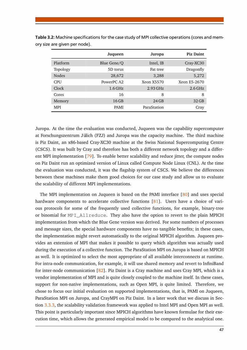
Table 3.2: Machine specifications for the case study of MPI collective operations (cores and mem-ory size are given per node).
Juqueen Juropa Piz Daint
Platform Blue Gene/Q Intel, IB Cray-XC30
Topology 5D torus Fat tree Dragonfly
Nodes 28,672 3,288 5,272
CPU PowerPC A2 Xeon X5570 Xeon E5-2670
Clock 1.6 GHz 2.93 GHz 2.6 GHz
Cores 16 8 8
Memory 16 GB 24 GB 32 GB
MPI PAMI ParaStation Cray
Juropa. At the time the evaluation was conducted, Juqueen was the capability supercomputer
at Forschungszentrum Jülich (FZJ) and Juropa was the capacity machine. The third machine
is Piz Daint, an x86-based Cray-XC30 machine at the Swiss National Supercomputing Centre
(CSCS). It was built by Cray and therefore has both a different network topology and a differ-
ent MPI implementation [79]. To enable better scalability and reduce jitter, the compute nodes
on Piz Daint run an optimized version of Linux called Compute Node Linux (CNL). At the time
the evaluation was conducted, it was the flagship system of CSCS. We believe the differences
between these machines make them good choices for our case study and allow us to evaluate
the scalability of different MPI implementations.
The MPI implementation on Juqueen is based on the PAMI interface [80] and uses special
hardware components to accelerate collective functions [81]. Users have a choice of vari-
ous protocols for some of the frequently used collective functions, for example, binary-tree
or binomial for MPI_Allreduce. They also have the option to revert to the plain MPICH
implementation from which the Blue Gene version was derived. For some numbers of processes
and message sizes, the special hardware components have no tangible benefits; in these cases,
the implementation might revert automatically to the original MPICH algorithm. Juqueen pro-
vides an extension of MPI that makes it possible to query which algorithm was actually used
during the execution of a collective function. The ParaStation MPI on Juropa is based on MPICH
as well. It is optimized to select the most appropriate of all available interconnects at runtime.
For intra-node communication, for example, it will use shared memory and revert to InfiniBand
for inter-node communication [82]. Piz Daint is a Cray machine and uses Cray MPI, which is a
vendor implementation of MPI and is quite closely coupled to the machine itself. In these cases,
support for non-native implementations, such as Open MPI, is quite limited. Therefore, we
chose to focus our initial evaluation on supported implementations, that is, PAMI on Juqueen,
ParaStation MPI on Juropa, and CrayMPI on Piz Daint. In a later work that we discuss in Sec-
tion 3.3.3, the scalability validation framework was applied to Intel MPI and Open MPI as well.
This point is particularly important since MPICH algorithms have known formulae for their exe-
cution time, which allows the generated empirical model to be compared to the analytical one.
47

Open- source, PAMI-based algorithms also provide analytical models for their execution time,
thus allowing us to get clear expectations about their performance.
Vendor implementations of MPI are quite strongly coupled to the actual machine. Comparing
them to a non-native MPI implementation would be unfair since the latter cannot use specialized
vendor hardware to run faster. Therefore, instead of evaluating different implementations on
the same machine, we looked at native implementations on different machines. It is important
to remember that different machines have different network topologies that can have different
network latencies and contention points. On Juqueen, the 5D torus topology and the built-in
messaging unit (MU) component allow for higher bandwidth and lower latency compared to
more conventional 3D torus and fat-tree topologies [81]. Therefore, each native implementa-
tion should be considered separately and compared to corresponding analytical models rather
than to an implementation on a different machine.
All three machines in our experiments provide highly accurate, high-resolution hardware cy-
cle counters in the form of registers that can be read very quickly with an atomic instruction:
MFTB on PowerPC, and RDTSC on x86. All the experiments were performed with a fixed CPU
frequency, and to obtain execution time the frequency was multiplied by the cycle count. With-
out these registers, which allow us to measure execution times with high-precision, one would
use a less accurate approach, that is, measure the runtime of N repetitions of a function and
then divide it by N to obtain an average. This approach suffers from pipeline effects and tends to
underestimate the latency [76]. We note that the experiments on Piz Daint were performed with
default Cray MPI library optimizations. Newer versions of Cray MPI have additional algorithms
that may improve scaling and can be used by setting appropriate environment variables.
We chose to set the number of MPI processes per node to be the same as the number of cores in
the node. The reason is that oversubscribing, namely running more processes than the number
of cores, can cause network contention at the node level. On the other hand, undersubscribing,
namely having fewer processes, can potentially cause insufficient utilization of the node’s com-
putational resources. This is because the adoption of multithreaded programming models is
neither ubiquitous among HPC applications nor can every application readily benefit from mul-
tithreading. For all the machines the range of MPI ranks was p = {26, 27, 28, 29, 210, 211, 212}.
Analysis of the results
Tables 3.3 and 3.4 present the results of our analysis. Both tables show the generated models
next to our expectations. Table 3.3 refers to runtime and Table 3.4 to memory metrics. Since
the size of the memory growth coefficients may be significant, we show full models of memory
overheads and estimated memory consumption by MPI. The R2 row lists the adjusted coefficient
of determination, which indicates how well the data fits a statistical model. It is used in the
model generation phase to create models that fit the data better [43]. Note that R2 is not
applicable to constant models. Following R2 is the row with the divergence models δ as defined
in Section 3.2.4. Finally, the match row specifies whether the generated model meets our
expectations. If the two are in agreement, a checkmark Ø is shown. If the match is approximate
according to the definition in Section 3.2.4, an approximation sign ≈ is shown.
48

Table 3.3: Generated (empirical) runtime models of MPI collective operations on Juqueen, Juropa, and Piz Daint alongside their theoretical expec-tations.
Barrier Bcast Reduce Allreduce Gather Allgather Alltoall Bcast (BT)
Juqueen
Expectation O (log p) O (log p) O (log p) O (log p) O (p) O (p) O (p log p) O (log p)Model O (log p) O (log p) O (log p) O (log p) O (p) O (p) O (p) O (log p)R2 0.99 0.86 0.93 0.87 0.99 0.99 0.99 0.99
δ(p) O (1) O (1) O (1) O (1) O (1) O (1) O (1/ log p) O (1)Match Ø Ø Ø Ø Ø Ø ≈ Ø
Juropa
Expectation O (log p) O (log p) O (log p) O (log p) O (p) O (p) O (p log p) O (log p)Model O (p0.67 log p) O (pp) O (pp log p) O (pp) O (p) O (p) O (p1.25) O (p1.25 log p)R2 0.99 0.98 0.99 0.99 0.99 0.98 0.99 0.99
δ(p) O (p0.67) O (pp/ log p) O (pp) O (pp/ log p) O (1) O (1) O (p0.25/ log p) O (p1.25)Match x ≈ ≈ ≈ Ø Ø ≈ x
Piz Daint
Expectation O (log p) O (log p) O (log p) O (log p) O (p) O (p) O (p log p) O (log p)Model O (p0.33) O (pp) O (pp log p) O (p0.67 log p) O (p) O (p1.25) O (p1.33) O (p log p)R2 0.99 0.94 0.94 0.99 0.99 0.99 0.99 0.99
δ(p) O (p0.33/ log p) O (pp/ log p) O (pp) O (p0.67) O (1) O (p0.25) O (p0.33/ log p) O (p)Match ≈ ≈ ≈ x B Ø ≈ ≈ x
49

A solid x represents an unquestionable mismatch. A warning sign B indicates the violation
of a performance guideline. Figure 3.5 depicts the runtime models for the collective functions
we benchmarked. The circles, squares, and triangles depict the actual measurements, whereas
the lines are the predictions. Each curve is annotated with the corresponding model that sits
on top of the curve. Since we focus on the scalability behavior of the models, we chose not to
show the constant terms. The discussion below starts with Juqueen, on which almost all the
generated models correspond almost fully to expectations. We then continue with Juropa and
Piz Daint, on which the results differed from our expectations to some degree.
Juqueen. On Juqueen, the performance of collective functions was generally better than on
the other machines and we found that almost all of our expectations were met. All the models
on Juqueen are either logarithmic or linear with respect to the number of processes p. As can
be seen in Table 3.3, all the generated models on Juqueen correspond exactly to the expected
models with the exception of MPI_Alltoall, which is identified as linear when, in fact,
the expectation would be O (p log p). The difference between reality and expectation is small
enough to be explained by noise and other system effects. The manually implemented binary-
tree (BT) version of the broadcast is shown in the rightmost column of Table 3.3. The expected
cost of this algorithm for small messages is: (α+ β) log p; and though it is slower in absolute
terms than the native MPI_Bcast, the generated model is still logarithmic. Table 3.4 presents
the models for the communicator memory overheads and the estimated fraction of the memory
allocated by the process that is consumed by MPI. Although the generated models on Juqueen
correspond to the expectations, the linear growth of some of the communicator constructors
can still become an issue at very large scale.
Juropa and Piz Daint. On Juropa and Piz Daint, the predicted performance models of some
collective functions did not fully match their expectations. These discrepancies between pre-
dicted and expected behavior suggest potential scalability issues. Almost all the generated
models, including the ones for MPI_Barrier, MPI_Bcast, and MPI_Reduce, did not
correspond to the expected logarithmic models. The generated model of the binary-tree (BT)
broadcast falls outside the deviation limits and clearly fails to match the expected logarithmic
model, too. Since we have a clear understanding of this algorithm and its complexity, we can
point to a number of external factors as potential causes of this discrepancy:
1. The network model that was used to calculate the expected cost of the binary-tree broad-
cast algorithm is a simplistic abstraction of a real-world network such as the IB fat-tree
interconnect on Juropa.
2. Network hardware and topology can influence the runtime of various collective functions
and make them slower than expected [83, 84].
3. On some machines, the performance of applications that use communication extensively
strongly depends on the node allocation they receive and the neighborhood of each
node [85]. An application that runs on a neighbor node and produces heavy network
load creates more perturbation for our benchmark.
50

512 1024 2048 40960
50
100
150
200
250
300
350
0.1 log2 x
0.1x0.67 log2x
2.11x0.33
Processes
Tim
e[µ
s]JuqueenJuropa
Piz Daint
(a) Barrier
512 1024 2048 40960
40
80
120
160
200
240
0.11 log2 x
3.39p x
1.06p
x
Processes
Tim
e[µ
s]
JuqueenJuropa
Piz Daint
(b) Bcast
512 1024 2048 4096
40
80
120
160
200
0.14 log2 x
0.23p x log2
x
0.1p x log2 x
Processes
Tim
e[µ
s]
JuqueenJuropa
Piz Daint
(c) Reduce
512 1024 2048 40960
150
300
450
600
750
0.13 log2 x
12.1p x
0.04x0.67 log2 x
Processes
Tim
e[µ
s]
JuqueenJuropa
Piz Daint
(d) Allreduce
512 1024 2048 4096
400
800
1200
1600
2000
0.46x
0.32x
0.11x
Processes
Tim
e[µ
s]
JuqueenJuropa
Piz Daint
(e) Gather
512 1024 2048 4096
1500
3000
4500
6000
7500
9000
0.63x
2.14x
0.16x1.25
Processes
Tim
e[µ
s]
JuqueenJuropa
Piz Daint
(f) Allgather
512 1024 2048 40960
1000
2000
3000
4000
5000
6000
6.26 log2 x
0.13
x1.
25lo
g 2x
0.03x log2 x
Processes
Tim
e[µ
s]
JuqueenJuropa
Piz Daint
(g) Bcast (BT)
512 1024 2048 40960
40
80
120
160
200
0.39x
16.8
3x1.
25
0.78x1.33
Processes
Tim
e[µ
s](m
ulti
plie
dby
10−3
)
JuqueenJuropa
Piz Daint
(h) Alltoall
Figure 3.5: Measurements (circles, squares, triangles) and generated runtime models (plot lines)on Juqueen, Juropa, and Piz Daint.
51

Table 3.4: Generated (empirical) models of memory overheads on Juqueen, Juropa, and PizDaint alongside their theoretical expectations.
MPI memory Comm_create Comm_dup Win_create Cart_create
Expect. O (1) O (p) O (1) O (p) O (p)Juqueen
Model 10.7 · 10−3 · log p 2.2 · 105 + 24 · p 2.2 · 105 96 · p 2.2 · 105 + 52 · pR2 0.72 1 − 1 0.99
δ(p) O (log p) O (1) O (1) O (1) O (1)Match ≈ Ø Ø Ø Ø
Juropa
Model 16+ 55 · p 264+ 28 · p 256 256+ 60 · p 356+ 24 · pR2 1 1 − 1 1
δ(p) O (p) O (1) O (1) O (1) O (1)Match x Ø Ø Ø Ø
Piz Daint
Model 46+ 1.35 · log p 3770+ 46 · p 3770+ 18 · p 3287+ 118 · p 2545+ 63 · pR2 0.23 0.99 0.99 0.99 0.99
δ(p) O (log p) O (1) O (p) O (1) O (1)Match ≈ Ø x Ø Ø
4. System noise and jitter could potentially be significant factors that influence the perfor-
mance [86, 87]. These factors mostly affect Juropa, since it does not have a specialized
kernel that has been optimized for noise reduction.
The performance models of MPI_Gather on both Juropa and Piz Daint, as well as the
MPI_Allgather model on Juropa, are linear as expected. On Piz Daint, however, the per-
formance model of the latter does not match the expectation, but still falls within the deviation
limits. In Table 3.3, the warning sign under Match signals that a performance guideline vi-
olation was detected. As discussed in Section 3.3.1, the automatic validation evaluates two
performance guidelines, one for Allreduce and one for Allgather. Although the actual measure-
ments on Piz Daint do not violate the Allreduce guideline, the generated models predict that the
guideline would be violated at larger scales. Note that a performance guideline violation does
not imply whether there is a mismatch or an approximate match to the expectation.
The communicator memory overheads on Juropa and Piz Daint are presented in Table 3.4.
On Juropa, the generated models correspond to expectations, and the initial overheads (the
constants) are very small. This is in direct contrast to Juqueen, on which these constants are
much higher. The model for communicator duplication on Piz Daint is linear, although it is
expected to be constant. The development team at Cray confirmed that the implementation
of MPI_Comm_dup was taken from MPICH 3.1.2 and that the MPICH version behaves in the
same manner. This result clearly shows that there might be a scalability bug in this function;
further work is required to find ways to fix it.
52

512 1024 2048 40960
500
1000
1500
2000
2500
0.01 log2 x
0.56x
1.35 log2 x
Processes
MB
JuqueenJuropa
Piz Daint
Figure 3.6: Measurements (circles, squares, triangles) and generated MPI memory consumptionmodels (plot lines) on Juqueen, Juropa, and Piz Daint.
Figure 3.6 presents the models for the resident memory size of an MPI process on all three
machines. In the case of Juropa, the generated model reveals a severe scalability problem. Even
with smaller values of p, it is non-scalable. Starting with 1024 nodes, it is impossible to have
8 MPI processes per node since all the processes would require 35 GB in total and the node’s
memory is just 24 GB. Our experiments confirmed this memory wall: memory allocation failed
when the total number of processes was 8192 (with 8 processes per node). Our findings are
confirmed by the documentation; the reason for the linear increase in allocated memory is that
ParaStation MPI uses by default the Reliable Connected (RC) InfiniBand service, which needs
0.55 MB of memory for each MPI connection [82]. When using MPI_Alltoall each process
will allocate 0.55p MB of memory, which is exactly the linear behavior we discovered through
our scalability validation framework.
3.3.3 Intel MPI and Open MPI
This subsection presents an evaluation of two additional implementations of MPI collective
operations, namely Intel MPI and Open MPI. The evaluation was carried out by Patrick Reisert
as part of his masters thesis [74], which was supervised by the author of this dissertation. Reisert
followed the same workflow as described in Section 3.3.1, but used a different benchmark (step
2), which will be described in more detail below. Unlike the initial evaluation that used three
different machines, Intel MPI and Open MPI were evaluated on the same system, that is, the
Lichtenberg cluster at the Technische Universität Darmstadt [88]. There were no additional
MPI implementations (e.g., MPICH) available on this system.
The first step in the workflow, in which expectations are defined, stays mostly the same.
The focus is on the same latency-oriented execution time, but without memory overhead of
communicator-related functions and MPI memory consumption. Reisert chose to evaluate the
same set of MPI collective operations, that is Barrier, Bcast, Reduce, Allreduce, Gather, Allgather,and Alltoall, so the expectations in Table 3.1 still apply. The third and the fourth step, namely
the generation of models and the validation of expectations, respectively, stay the same as well.
53

Table 3.5: Generated (empirical) runtime models of Intel MPI and Open MPI collective opera-tions alongside their theoretical expectations.
Barrier Bcast Reduce Allreduce Allgather Alltoall Bcast (BT)
Expect. O (log p) O (log p) O (log p) O (log p) O (p) O (p log p) O (log p)
Intel MPI
Model O (p) O (p0.75 log2 p) O (p0.75 log p) O (log p) O (p2.75) O (p log p) O (log p)R2 0.99 0.99 0.97 0.74 0.99 0.99 0.92
δ(p) O (p/ log p) O (p0.75 log p) O (p0.75) O (1) O (p1.75) O (1) O (1)Match x x x Ø x Ø Ø
Open MPI
Model O (log2 p) O (log p) O (log2 p) O (log p) O (p log2 p) O (p log p) O (log2 p)R2 0.99 0.99 0.99 0.99 0.99 0.99 0.99
δ(p) O (log p) O (1) O (log p) O (1) O (log2 p) O (1) O (log p)Match ≈ Ø ≈ Ø ≈ Ø ≈
Benchmark design
Following recent studies on MPI benchmarking accuracy [89], Reisert uses the ReproMPI bench-
mark [90] rather than the benchmark suggested earlier in Section 3.3.1. Although the basic
structure of ReproMPI resembles our earlier benchmark, it features an improved version of the
window-based synchronization technique, as well as a flexible mechanism for predicting the
number of repetitions that are required to obtain statistically sound results. Reisert configured
ReproMPI to use the same timing mechanism suggested earlier, namely the RDTSC register
available on x86 platforms and a fixed clock frequency. By default, ReproMPI outputs the run-
time of an operation for each process. To be consistent with the benchmark in Section 3.3.1, an
additional script was used to find the maximum result across all the processes.
Evaluation
The benchmarks were executed on a separate island of 32 nodes on Lichtenberg. Each node
comprises two Intel Xeon E5-2670 processors with 8 cores (hyper-threading disabled) and 16
GB of memory, which means 16 cores and 32 GB of memory per node. Reisert used the
same configuration of one MPI process per core as before and the range of MPI ranks was
p = {16, 32, 64, 128, 256, 512}. Following the observations in Section 3.3.2, the whole is-
land was reserved for each benchmark run. This ensured that no other program used resources
within this island and the negative effects of a busy neighborhood [85] were eliminated.
Analysis of the results
Table 3.5 shows the evaluation results. The rows follow the same format as in Table 3.3. Note
that MPI_Gather is missing from the table because the results indicated that both Intel MPI
54

3264 128 256 5120
25
50
75
100
125
150
0.079x
1.13 log22
x
Processes
Tim
e[µ
s]Intel MPIOpenMPI
(a) Barrier
3264 128 256 5120
0.2
0.4
0.6
0.8
1.0
1.2
0.13x0.75 log
22x
11.26 log2 x
Processes
Tim
e[m
s]
Intel MPIOpenMPI
(b) Bcast
3264 128 256 5120
10
20
30
40
50
60
0.03x0.75 log2x
0.32 log22
x
Processes
Tim
e[µ
s]
Intel MPIOpenMPI
(c) Reduce
3264 128 256 5120
50
100
150
200
250
11.38 log2 x
19.88 log2 x
Processes
Tim
e[µ
s]
Intel MPIOpenMPI
(d) Allreduce
3264 128 256 5120
2
4
6
8
10
12
14
4.5 · 1
0−4 x
2.75
0.07x log22
x
Processes
Tim
e[m
s]
Intel MPIOpenMPI
(e) Allgather
3264 128 256 5120
10
20
30
40
50
60
3.65 log2 x
0.42 log22x
Processes
Tim
e[µ
s]
Intel MPIOpenMPI
(f) Bcast (BT)
3264 128 256 5120
3
6
9
12
15
18
0.73x log2 x
3.43x log 2x
Processes
Tim
e[m
s]
Intel MPIOpenMPI
(g) Alltoall
Figure 3.7: Measurements (circles, squares) and generated runtime models (plot lines) of someof the collective operations in Intel MPI and Open MPI.
55

and Open MPI changed the underlying algorithm of this operation when the number of pro-
cesses was increased. At the time of the study, we were unable to find a way to disable the
algorithm switch. This is an example for a use case for the segmented modeling approach [59]
that aims to solve the problem where the algorithm changes its behavior substantially for some
range of the input parameter. A substantial change means that a different model is needed
to explain the new behavior. In other words, the measurements cannot fit accurately just one
model, hence, we need to find an inflection point or possibly a number of inflection points and
fit a different model for each segment between these points. The segmented modeling tech-
nique tries different potential inflection points and checks whether the two new models give
us a better fit. Naturally, this approach requires using more values for the input parameter,
since each segment is smaller than the whole range of values we have. In our case, however,
the maximum number of processes per island is 512, which means increasing the number of
processes would have required using two separate islands and this would have exacerbated the
influence of the network topology on the measured runtime [83, 84].
Intel MPI. In the case of Intel MPI, about half of all the predicted performance models do
not match the expectations. MPI_Bcast and MPI_Allgather are particularly problematic.
Figures 3.7b and 3.7e demonstrate that the models for these operations grow much faster than
the corresponding models for Open MPI, which are closer to the expectations. The last column
of Table 3.5 shows the Intel MPI model for the binary-tree (BT) version of the broadcast opera-
tion. The implementation of this litmus test is based on MPI point-to-point communication, and
since the benchmarks were performed on a separate, exclusively reserved island, the results
clearly point to potential implementation issues in Intel MPI. In the case of MPI_Barrier
and MPI_Reduce, Figures 3.7a and 3.7c show that the execution times of Intel MPI are better
or on par with Open MPI. Furthermore, the predicted models have relatively small coefficients.
This means that the mismatch in this case is most likely caused by OS jitter and noise in general,
rather than by implementation issues.
Open MPI. In the case of Open MPI, there are no mismatches at all and almost half of the
models correspond to the expectations. Table 3.5 shows that the model for the binary-tree (BT)
version of the broadcast operation is slightly worse than expected. Since the benchmarks were
executed on a separate island of Lichtenberg, network interference was not a factor in this case.
Lichtenberg nodes do not have a specialized kernel, thus the likely cause of discrepancies is OS
jitter [87].
From the Intel MPI and Open MPI results it is not possible to derive any conclusion as to
how well either of these MPI implementations perform relative to MPICH, which is the basis
for the MPI implementations in Section 3.3.2. The reason is that the evaluation was performed
on different machines and under different conditions (e.g., unique networking hardware on
Juqueen and separate island of 32 nodes on Lichtenberg).
3.4 Further Evaluation of the Validation Framework
MPI collective operations are an important case study that demonstrates the strengths of the
scalability validation framework. However, our scalability validation approach targets HPC
56

Table 3.6: Generated (empirical) runtime models of MAFIA functions alongside their theoreticalexpectations.
gen dedup pcount unjoin
Expectation O (k32k) O (k42k) O (k2k) O (k32k)Model O (k42k) O (k42k) O (k2k) O (k22k)δ(k) O (k) O (1) O (1) O (1/k)Match ≈ Ø Ø ≈
libraries in general and is applicable to many use cases. In this section, we present further
examples in which the framework is used to validate performance expectations.
3.4.1 MAFIA
No matter how large the degree of parallelism, optimizing sequential code is still essential
to achieve good performance. The subject of our next case is therefore MAFIA (Merging of
Adaptive Finite IntervAls), a sequential data-mining program utilizing a collection of key rou-
tines [70]. One of the basic problems in data mining is identifying regions of similarity in a
multi-dimensional data set. Many applications, however, exhibit a high degree of dimension-
ality in the data, which makes traditional approaches of all-attribute clustering problematic. A
possible solution is to use subspace clustering methods to identify clusters in a subset of dimen-
sions. MAFIA is one example of such a method. It is a serial algorithm for subspace clustering
based on adaptive grid methods [70]. The cluster dimensionality k is a critical parameter in this
algorithm since the ultimate goal is to identify clusters across all dimensions. Users of MAFIA
will start with a smaller k but will be interested in increasing it to catch all the dimensions. We
are interested in applying our framework to see whether the scaling expectations as a function
of k are valid. This use case is an example of algorithmic modeling since the model parameter
k is a parameter of the algorithm itself.
Following the four steps of our approach, we start by defining the expectations. Along with
k, the parameters of MAFIA are the number of data points n, the dimensionality of the points d,
and the number of clusters m. We further identify four main functions (i.e., kernels) in the main
computation phase of MAFIA: (i) gen—generation of candidate sets; (ii) dedup—de-duplication
of the sets; (iii) pcount—identification of dense sets; and (iv) unjoin—determination whether
lower dimensional sets were not already absorbed by the higher ones [91].
Table 3.6 presents the expectations for these functions provided by Adinetz et al. [70] in their
effort to optimize MAFIA. In contrast to the MPI study, all the expectations are exponential:
O (k2k), O (k32k), and O (k42k). The focus in this use case was the runtime of the algorithm as
k increases; therefore we set the other parameters as follows: n= 105, d = 20, and m= 3. The
benchmarking process was much simpler in this case since MAFIA is a serial code and we were
not modeling scalability on an increasing number of cores. In other words, the experiments were
conducted on one node of Juropa and repeated for k = 3, 4, ..., 16. In all of these experiments
we did not change the default deviation limits or the search space boundaries. As Table 3.6
57

shows, all the generated models match our expectations completely or are inside the deviation
limits. This example illustrates the flexibility of our approach, which can be adapted to different
scalability problems with different expectations.
3.4.2 OpenMP
As already discussed in Chapter 1, OpenMP is an important programming model for shared-
memory systems. It is also one of the approaches to program accelerators, such as Xeon Phi.
As a result, HPC applications increasingly adopt OpenMP and combine it with MPI in a hybrid
approach that aims to exploit both intra-node and inter-node parallelism. It is important then
to analyze the scalability behavior of the basic, and most essential, OpenMP constructs as the
number of threads is increased.
This subsection is based on the study of OpenMP scalability carried out by Iwainsky et al. [53]
in collaboration with the author of this dissertation. Specifically, he adapted the window-based
synchronization mechanism [77] described earlier to OpenMP threads (the benchmarking ap-
proach discussion below provides more details). Iwainsky et al. used step 3 (generation of scal-
ing models) and to some extent step 2 (benchmarking) from the scalability validation workflow.
In other words, the benchmarking approach borrowed key ideas from the approach described
in Section 3.3.1. The goal was to evaluate the scalability of OpenMP constructs parallel, barrier,and for. In this section, however, we show that this evaluation can be viewed as another use
case of our framework to validate performance expectations.
Expectations
The first step in the workflow requires us to choose the metric and the evaluated functions, as
well as identify our performance expectations. In this case, the metric is execution time and
the generated models are functions of the number of threads used for execution, which we
denote as p. The functions represent execution times of five different construct configurations,
namely: parallel, parallel firstprivate, barrier, for static, and for dynamic. The second construct
is a parallel construct with a firstprivate clause, the fourth and the fifth are for constructs with
static and dynamic clauses, respectively (see Section 1.2 for an overview of OpenMP constructs).
We can derive the expectations from analyzing the implementation approaches. A very simple
parallel construct implementation has linear complexity (O (p)), since the main thread has to
invoke a thread creating call, such as pthread_create, for every thread that participates in
the parallel region. An optimized implementation will create a thread pool in advance, thereby
leaving only minimal initialization code in the parallel construct. Without the thread creation
overhead, this option would be much faster, but it would still have to initialize every thread it
gets from the pool. In other words, it would still have linear complexity.
The meaning of the firstprivate clause is that the OpenMP runtime has to copy a value (or
values, in the case of an array) into a private variable in each thread. This resembles a broadcast
operation between threads, and as we discussed in the MPI case study, the runtime expectation
58

of this algorithm is logarithmic. Even if we used a thread pool, the expectation of the parallelfirstprivate construct would be logarithmic (O (log p)).
A simple implementation of the barrier construct as a centralized barrier will result in linear
complexity, since each thread busy-waits for a shared flag, contributing to increased contention.
We can expect that a good implementation of an OpenMP runtime will use a more efficient
barrier [92] that has a logarithmic complexity. The for construct with a static clause should
have lower complexity compared to a for with dynamic clause. The static scheduling approach
assigns portions of the loop to threads just once in the beginning of the loop, whereas dynamic
scheduling assigns chunks of the loop to the threads repeatedly. Once a thread finishes executing
a chunk, the control returns to the OpenMP runtime that decides which chunk it should assign
to the current thread next. Dynamic scheduling greatly improves load balancing, but at the
cost of higher overhead. The complexity of the static scheduling, therefore, should be constant
(O (1)), whereas for dynamic scheduling it should be linear (O (p)).
Benchmarking approach
The benchmarking approach used by Iwainsky et al. [53] is based on the EPCC OpenMP bench-
marking suite [93]. The suite is a comprehensive collection of micro-benchmarks that cover
a large selection of OpenMP constructs and has been designed to evaluate the parallelization
overhead. The overhead is computed by first running a workload without OpenMP and then
with specific OpenMP construct and then calculating the difference between the two runs. Ex-
ecution times of constructs are not measured directly, but computed by measuring the runtime
of multiple repetitions and then dividing by the number of repetitions.
Although the EPCC benchmarks are good for understanding OpenMP overheads, the mea-
surement technique is not precise enough for producing performance models from the results.
Therefore, Iwainsky et al. adapted the EPCC suite to resemble the benchmark used in the MPI
case study (see Section 3.3.1). Specifically, they used the window-based synchronization mech-
anism [77] to ensure that all the threads enter the benchmarked construct at the same time.
They also collected the individual execution times of each construct in each thread and reduced
them, across all of the threads, to a single maximum or minimum value.
The benchmarks were executed on one node of the BCS cluster [94] at RWTH Aachen Uni-
versity, on a Xeon Phi 7120 (Knights Corner) accelerator, and on a node of Juqueen [52], an
IBM Blue Gene/Q machine at Forschungszentrum Jülich (FZJ). The BCS cluster provides larger
shared-memory super-nodes by using Bull’s Coherent Switch chips that transform 2 or 4 physi-
cal nodes into one NUMA system with up to 128 cores. Since each node has multiple sockets,
each super-node has two NUMA levels that can lead to increased execution times. With up
to 61 cores, the Xeon Phi accelerator also provides a higher number of cores. But unlike the
BCS super-node, it has a flat hierarchy with uniform access times to the on-accelerator mem-
ory. A Blue Gene/Q node has 16 compute cores with a 4-way simultaneous multithreading
(SMT) for each core. On the BCS super-node, three different OpenMP runtimes were used:
GNU OpenMP [95], Intel OpenMP Runtime Library [96], and PGI. In the case of Xeon Phi, the
59

authors used only the native Intel runtime, and on a Blue Gene/Q node only the native IBM
runtime.
The measurements were carried out on an increasing number of threads with each thread run-
ning on a separate core. Iwainsky et al. [53] discovered different behavior depending whether
the number of threads was a power-of-two or a multiple of 16 (with or without an offset of 8
threads). Our goal in presenting this study is to show that it can be viewed as a use case of the
scalability validation framework. Therefore, we choose brevity over breadth and focus only on
the power-of-two thread counts.
Analysis of the results
Table 3.7 presents the results of the evaluation. It was adapted from the results by Iwainsky
et al. [53] and follows the same format as Table 3.3. It is separated into five sections: the
GNU, Intel, and PGI OpenMP runtimes on the BCS cluster, a Xeon Phi platform, and a Juqueen
node. Each section shows the expected models, the generated models, the adjusted coefficient
of determination R2, the divergence models, and the match criteria.
The GNU and Juqueen runtimes show the worst scalability behavior with at least three cases
in which the generated models mismatch their expectations. Surprisingly, the barrier and the
for static constructs have particularly poor performance. By comparing the GNU results to the
Intel results, which are based on the same hardware, we can conclude that the GNU runtime
has scalability issues in its implementation. Although the Blue Gene/Q hardware provides
better support for parallelism, with features such as atomic operation in the L2 cache [6], it
is difficult to attribute the poor scalability behavior to any single reason. It can be related to the
implementation, but it also might be related to the combination of the unique hardware and the
kernel (CNK). For example, since each core has a 4-way SMT, a close binding would result in
four threads running on the same physical cores. This might introduce unexpected contention
effects that have a negative impact on scalability.
The Intel runtime on the BCS cluster shows the best scalability behavior with all the generated
models matching either exactly or approximately the expectations. Incidentally, this runtime
was made open-source and subsequently incorporated into the LLVM OpenMP runtime. It is
regularly updated, and widely used both in academia and industry. The model for the parallelconstruct is logarithmic and asymptotically better than the expected linear model. It uses a
thread pool and probably some other optimizations as well. The PGI results are not as good as
the Intel ones, but they are better than the GNU results and on par with Xeon Phi. Surprisingly,
in the case of Xeon Phi, the for dynamic construct is much better than the for static construct. It
is difficult to explain this phenomenon, but one reason might be the low R2, which means the
model does not fit the measured behavior well enough.
The OpenMP scalability study is another example how the scalability validation framework
can be used to validate performance expectations. The results show that we can evaluate dif-
ferent implementations running on the same hardware and identify potential scalability issues
in each implementation.
60

Table 3.7: Generated (empirical) runtime models of the evaluated OpenMP constructs alongsidetheir theoretical expectations (based on data from Iwainsky et al. [53])
.
Parallel Firstprivate Barrier Static Dynamic
Expectation O (p) O (log p) O (log p) O (1) O (p)BCS Cluster (GNU)
Model O (p1.25) O (p) O (p1.33 log p) O (p1.33 log p) O (p1.25 log p)R2 0.99 0.99 0.99 0.98 0.99
δ(p) O (p0.25) O (p/ log p) O (p1.33) O (p1.33 log p) O (p0.25 log p)Match ≈ x x x ≈BCS Cluster (Intel)
Model O (log p) O (log p) O (p0.25) O (log p) O (p)R2 0.78 0.94 0.98 0.84 0.99
δ(p) O (log p/p) O (1) O (p0.25/ log p) O (log p) O (1)Match Ø Ø ≈ ≈ Ø
BCS Cluster (PGI)
Model O (p0.67 log p) O (p0.67) O (log2 p) O (log p) O (p1.25 log p)R2 0.99 0.99 0.95 0.62 0.99
δ(p) O (p−0.33 log p) O (p0.67/ log p) O (log p) O (log p) O (p0.25 log p)Match Ø x ≈ ≈ ≈Xeon Phi
Model O (p0.67) O (p0.67) O (pp) O (p1.5) O (p0.25)R2 0.97 0.98 0.99 0.75 0.65
δ(p) O (p−0.33) O (p0.67/ log p) O (pp/ log p) O (p1.5) O (p−0.75)Match Ø x ≈ x Ø
Juqueen
Model O (p1.25) O (p1.25) O (p1.33 log p) O (p2.33) O (p2.33)R2 0.99 0.99 0.99 0.99 0.99
δ(p) O (p0.25) O (p1.25/ log p) O (p1.33/ log p) O (p2.33) O (p1.33)Match ≈ x x x x
3.4.3 Parallel sorting algorithms
In this subsection, we present another use case for the scalability validation framework, namely
validation of performance expectations of parallel sorting algorithms. In general, parallel sort-
ing focuses on techniques to solve the sorting problem using parallel processing [97, 98, 99].
Sorting is a fundamental problem in computer science and has many uses. However, with the
increasing scale of HPC systems the problems scientists and engineers focus on increase in scale
as well. In other words, the input for a sorting algorithm no longer fits into one node and we
need, therefore, to formulate the parallel sorting problem [25] in terms of distributed memory:
Input: A distributed sequence of n =∑p−1
i=0 |Ni| elements such that each block of elements Ni
has np elements and is assigned to process pi.
61

Figure 3.8: Parallel sorting based on finding exact splitters (from Siebert and Wolf [97]).
Output: A permutation of the distributed input sequence such that each process pi has a block
N ′i , in which all elements are sorted, and ∪p−1i=0 N ′i = ∪p−1
i=0 Ni. Moreover, for every i ≤ j we
have N ′i ≤ N ′j , where Ni ≤ N j means that every element of Ni is less than or equal to every
element in N j.
Our focus in this use case is on five parallel sorting algorithms: (i) Sample sort [25]; (ii) His-
togram sort [98]; (iii) Exact-splitting sort [97]; (iv) Radix sort [100]; and (v) Mini sort [101].
The first three are so called splitter-based algorithms. The fourth is a parallel variant of the
well-known sequential Radix sort [102], and the fifth algorithm addresses a special case of
the parallel sorting problem where np = 1. The initial work to evaluate the performance of
these algorithms was carried out by Yannick Berens as part of his bachelor thesis [103], which
was supervised by the author of this dissertation. To apply the scalability validation frame-
work, we developed a library with implementations of these algorithms called libparsort. As
a starting point, we used existing implementations of Sample sort, Exact-splitting sort, Radix
sort, and Mini sort created by Elmar Peise and Christian Siebert. We then refactored these im-
plementations and implemented Histogram sort from scratch, as well as added a number of
improvements to the Exact-splitting and Mini sort implementations. Note that since we studied
the available implementations in detail and also developed our own code, there was no need
for a performance litmus test as in the MPI case study.
62

Table 3.8: Runtime complexities of parallel sorting algorithms.
Algorithm Runtime complexity
Sample sort O ( np log n+ p2 log p)
Histogram sort O ( np log n+ rp log n
p )Exact-splitting sort O ( n
p log n+ p log2 n)Radix sort O ( b
k (np + 2k + log p))
Mini sort O (log2 p)
Solutions that try to gather too many elements in one node or that fail to exploit the available
parallel resources will not scale. Splitter-based algorithms address these two issues by first
letting processes sort their part of the input and then by solving the merging-redistribution
problem without relying on any one process in particular. Figure 3.8 shows the steps of Exact-
splitting sort [97], which is an example of a splitter-based algorithm. These algorithms have
a common scheme of four steps, namely, sorting the elements locally, finding p + 1 splitters
(the first and the last splitter are implicit and correspond to the minimum and maximum values
of the input), redistributing the elements according to the splitters, such that all the elements
between splitter si and si+1 end up in process pi, and finally, merging all the parts in process
pi locally. The main differences between the splitter-based algorithms is in the order of the
solution steps and the technique to find the splitters. A simple variant is the Sample sort [25]
algorithm. In this algorithm, each process i selects a sample of p−1 candidates from Ni, which
it sorts beforehand, and sends them to the root process. The root then sorts these candidates
and selects p + 1 splitters. Eventually it broadcasts the splitters back to the processes. The
main disadvantage in this algorithm is gathering and sorting the splitter candidates in one
process. As p increases this will become a significant bottleneck. Histogram sort circumvents
this bottleneck by selecting a random sample of splitter candidates across the whole range of
the input data. It then computes the prefix sum of local histograms based on the sample. The
prefix sum produces the location of each candidate within the eventual sorted array. This allows
the algorithm to check whether a candidate falls within the range of an ideal splitter ( splitter ilocation is n
p (i+1)). Histogram sort repeats this step until all the splitters are found. The range
is a parameter of the algorithm, but if we keep it reasonably small, blocks N ′i will have roughly
the same size in the end [98]. The Exact-splitting algorithm aims to find the exact splitters as
well, but instead of relying on histograms it uses an efficient scheme for approximating global
medians. By repeating this scheme for every splitter, it guarantees that we find exact splitters,
in other words, N ′i =np for each process. Although finding better splitters comes at the cost of
more communication steps, both Histogram and Exact-splitting sort eliminate the bottleneck in
the Sample sort algorithm.
Radix sort is not a comparison-based sorting algorithm. Instead it takes advantage of the
binary representation of the keys. The idea is to break the keys into digits of one or more bits,
and then sort one digit at a time. To work properly, the algorithm proceeds from the least
significant to the most significant bit using a stable sorting algorithm for each digit. In most
cases, Counting sort [102] is used to sort the digits, since it is stable and well suited for this
63

type of input. The parallel variant of Radix sort parallelizes the Counting sort by efficiently
counting in parallel using collective reduction operations in MPI.
Mini sort assumes that each process has just one element of input data, that is n = p. The
idea behind it is similar to Quicksort. Specifically, it uses an efficient scheme to approximate
the global median among a group of processes, which is then used as a pivot to partition the
processes into three groups: the ones with a smaller value than the pivot, the ones with an
equal value, and the ones with a higher value. After exchanging the data elements, the sorting
continues recursively in the first and third partitions and stops when a partition contains just
one element.
First implementations of Exact-splitting sort and Mini sort approximated global medians
based on a ternary tree selection proposed by Rousseeuw and Bassett [104]. However, for
more robustness and accuracy, the approximation method was changed to a binary tree-based
technique proposed by Axtmann and Sanders [99].
Expectations
The first step in the scalability validation workflow requires us to choose the metric and identify
the performance expectations of the algorithms. In this case, the metric is execution time and
the generated models are functions of the number of MPI processes p. Table 3.8 presents the
theoretical runtime complexities of the sorting algorithms [25, 97, 101, 102]. Note that the
three splitter-based algorithms have a common component O ( np log n) for the local sorting step,
but they differ in their approaches for finding the splitters. In the case of the Histogram sort,
r is the number of repetitions required for the splitter finding phase to converge. Radix sort
assumes that the input values are integers of b bits and it breaks these integers into digits of kbits. There are b
k digits and for each digit it runs a parallelized Counting sort [102]. Mini sort
works with minimal data (i.e., n= p) and therefore its complexity is based only on p.
Benchmarking approach
The second step in the scalability validation workflow instructs us to define the benchmarking
approach. Previous case studies adopted custom solutions to instrumentation that allowed
us to adhere to certain constraints and highlight specific aspects of performance (e.g., MPI
collective functions had to start at the same time). In the parallel sorting case, however, we can
adopt a more standard approach and use an existing instrumentation solution. Since our model
generation tool Extra-P (see Section 2.4) provides direct support for Score-P [36], Berens used
this instrumentation platform to instrument the sorting functions in the library. One advantage
of Score-P is that it measures execution times of the whole call tree, such that we obtain not
only the execution time of the sorting function itself, but also the times of the functions called
within that function. In other words, we can get models for every logical step of the algorithms
(e.g., local sorting, splitter finding, and so on).
The benchmarks were executed on two systems, the first one is Lichtenberg (see Sec-
tion 3.3.3) and the second one is Juqueen (see Section 3.3.2). On both machines, we used
64

Table 3.9: Generated (empirical) runtime models of five parallel sorting algorithms: Sample sort,Histogram sort, Exact-splitting sort, Radix sort, and Mini sort.
Sample Histogram Exact-splitting Radix Mini
k = 4 k = 8
Expect. O (p2 log p) O (p) O (p log2 p) O (log p) O (log p) O (log2 p)
Lichtenberg
Model O (p2 log p) O (p) O (p1.75 log p) O (pp) O (log2 p) O (p0.75 log2 p)R2 0.99 0.99 0.99 0.99 0.99 0.99
δ(p) O (1) O (1) O (p0.75/ log p) O (pp/ log p) O (log p) O (p0.75)Match Ø Ø ≈ ≈ ≈ x
Juqueen
Model O (p2 log p) O (p0.75) O (p log p) O (p1.25) O (log p) O (log2 p)R2 0.99 0.99 0.99 0.99 0.94 0.99
δ(p) O (1) O (p−0.25) O (1) O (p1.25/ log p) O (1) O (1)Match Ø ≈ Ø x Ø Ø
one MPI process per core. On Lichtenberg, p = {32, 64, 128, 256, 512} and on Juqueen,
p = {211, 212, 213, 214, 215, 216}. The input elements were 64-bit integers generated randomly
in uniform distribution. For Histogram sort, we also used the Gaussian distribution. The num-
ber of elements per process was set to be constant with np = 10M (except for Mini sort with
np = 1), which ensured that we modeled only the influence of p on the performance.
Analysis of the results
Table 3.9 presents the results of the evaluation. The expectations are leading order terms of
simplified expressions of the runtime complexities from Table 3.8. Since n= C p the expression
O ( np log n) turns into O (log p), and compared to other terms it is not the leading order one. In
Histogram sort, r depends on the distribution of the input data. We ran the evaluation both
with uniform and Gaussian distributions and in both cases r = 2. Therefore, we assume that ris constant in the expectation. In Radix sort, b and k do not change during the benchmarking
and are be considered constant, which means the expectation turns into O (log p). However,
depending on the value of k, the hidden constant coefficient could become quite large.
The models for Sample sort on both Lichtenberg and Juqueen match the expectation and re-
flect the splitter-finding complexity. Although on Lichtenberg the execution time of the splitter-
finding step was smaller than that of other steps, the model for this step is O (p2 log p) and
dominates the other steps.
The models for Histogram sort reflect both the evaluation with uniform and Gaussian distri-
butions. In both cases, the splitter-finding step converged after two iterations, which means the
models for both distributions are the same. The model for Lichtenberg matches the expectation,
whereas the model for Juqueen is actually better than the expectation.
In the case of Exact-splitting sort, the model for Lichtenberg does not match the expectation
exactly, whereas the model for Juqueen is an exact match. The reason is that Exact-splitting
65

sort requires more communication steps to find the splitters. Specifically, it runs the global
approximation step, which uses collective operations, for every splitter (i.e., p times). This
means it invokes a large number of collective operations in the splitter-finding step and any
potential overheads or inefficiencies are accumulated. Since Juqueen has highly optimized
collectives, the accumulated overhead is smaller compared to Lichtenberg and this results in a
performance model that matches the expectation.
We evaluated Radix sort with two different digit sizes, namely k = 4 and k = 8. Since the
input values were 64-bit integers (i.e., b = 64), the number of the Counting sort steps (i.e., bk )
was 16 and 8, respectively. A higher number of Counting sort steps is translated into a larger
constant coefficient in the expectation. Table 3.9 shows that for k = 4 the Juqueen model does
not correspond to the expectation, while the Lichtenberg model matches only approximately.
One possible explanation lies within the implementation of the Counting sort step, which is
based on MPI point-to-point communication. Counting sort determines the designated locations
of the digits in the global sorted array and uses point-to-point communication to exchange
the digits between the processes. Since there were much more processes on Juqueen than on
Lichtenberg, the cost of this communication is higher on Juqueen and this is reflected in the
generated model. For k = 8, the number of Counting sort steps was twice as small leading
to a reduced number of point-to-point operations. Besides, the memory consumption of our
implementation of the Counting sort step increases with k and p. This forced us to restrict the
process counts on Juqueen for k = 8 and use up to p = 214 processes. A smaller number of
processes reduces the cost of the point-to-point communication, which results in models that
match the expectations more closely.
The model for Mini sort on Lichtenberg does not match the expectation, whereas on Juqueen
there is an exact match. Since both Exact-splitting sort and Mini sort are based on global median
approximation, the reason for the non-matching models is similar. The difference between the
Lichtenberg model and the Juqueen model in both cases is the same as well, that is O (p0.75).
3.5 Summary and Conclusion
In this chapter, we propose a new software engineering approach for extreme-scale systems.
With our scheme, we identify scalability issues in libraries that are thought to be scalable and
pinpoint possible performance bugs and room for improvement. In contrast to previous ap-
proaches, our technique only requires the performance engineer to have a vague (asymptotic)
idea of the scalability, although the accuracy improves if more information is available (e.g.,
a performance litmus test or more precise expectations). We also supply a tool chain that au-
tomates large parts of our four-step process and is ready for immediate use by performance
engineers.
To achieve this, our tool chain utilizes empirical performance modeling to generate models
that describe the behavior of functions in a target HPC library. To understand the scaling be-
havior, users can model execution time as the number of processes increases, and divergence
models, derived from the generated models, reveal how severe the discrepancy between the ob-
served and expected performance is. We demonstrate the effectiveness of our mechanism using
66

a number of use cases, namely MPI collective operations, the MAFIA code, OpenMP constructs,
and parallel sorting algorithms.
Our first case study, however, is probably the most important library interface in HPC, that
is, the MPI library. We chose to focus on it first because many commercially mature and well-
tested implementations are available and clear performance expectations exist in the literature.
We show how our approach enables MPI developers to spot scalability bugs early on, before
commencing full-scale tests on the target supercomputer. For this, we used automated exper-
iments on four different machines with five different MPI libraries, and our tool discovered a
number of scalability issues that can be grouped into the following cases: (a) key collective
functions on Juropa and Piz Daint display unexpected behavior; (b) the performance guideline
All reduce � Reduce + Bcast is potentially violated on Piz Daint; (c) memory consumption on
Juropa limits the number of possible processes; (d) communicator duplication on Piz Daint
consumes more memory than necessary; and (e) on Lichtenberg, Open MPI generally has a
better scalability than Intel MPI. We conclude that our approach is a viable technique that can
both point to limitations of the systems and provide MPI developers with important hints for
improving the scalability of their implementations. We also expect that this will motivate the
development of clear performance expectations for other parallel libraries, such as ScaLAPACK
or the parallel BLAS.
67

4 Task Dependency GraphsIn this chapter, we discuss task dependency graphs (TDGs). It is based in part on a previous
paper by Shudler et al. [58] and will provide the necessary background for the discussion on
practical isoefficiency analysis in Chapter 5. We focus on techniques to build TDGs and analyze
them, as well as a method to replay the tasks in a TDG to simulate the execution of a task-based
application.
4.1 Graph Abstraction for Task-based Applications
There is an important difference between tasks and threads: a task is a work package contain-
ing a collection of instructions to be executed, whereas a thread is a light-weight process that
executes given instructions in an independent context. A task-based code can be executed by
one or more threads running on one or more cores. For the purpose of our discussion, we as-
sume that each instance of a task is executed at any given time by only one thread and that the
number of threads is equal to the number of cores (i.e., each thread runs on a separate core).
The execution of a task-based code can be represented as a directed acyclic graph (DAG)
G = (V, E), where the nodes V are tasks and the edges E represent dependencies between tasks.
Henceforth, we will refer to this DAG as a task dependency graph (TDG). An edge (v , u) ∈ Emeans that task u cannot begin execution before v finishes. This type of dependency is an
abstraction. It can either represent a data dependency [26] such as Read-After-Write (RAW),
Write-After-Read (WAR), and Write-After-Write (WAW), or a control dependency. In Figure 4.1,
which shows a small TDG with execution times for each task, a task with a runtime of 9 cannot
run before tasks with runtimes of 7 and 4 finish running. Except for some really simple cases,
most of the interesting and useful problems have numerous dependencies in their algorithm
flow, thereby producing non-trivial TDGs.
In the process of execution, the scheduler assigns tasks ready to be executed to threads.
Depending on the scheduler, tasks might be stopped (i.e., preempted) and resumed later. In
this situation, tasking environments, including OpenMP, distinguish between tied and untiedtasks. A tied task can only be executed by the thread that started executing it, meaning that if
this task is preempted, it can only be resumed by the thread that executed it before. An untied
task, on the other hand, can be resumed by any available thread after preemption. Both types of
tasks have advantages—tied tasks provide guarantees for private thread data (e.g., #pragma
omp threadprivate in OpenMP) [28], whereas untied tasks provide more flexibility to the
scheduler.
In the next sections, we present important metrics and rules that characterize TDGs, discuss
ways to construct and analyze TDGs, and eventually, present the task replay engine that allows
us to replay a TDG and simulate the execution of a task-based program.
69

�
� � �
� � � �
�
Figure 4.1: Task dependency graph; each node contains the task time and the highlighted tasksform the critical path.
4.1.1 Metrics and rules
We characterize TDGs using a set of key metrics [102, 105, 106]. The work of the computation
is the total execution time on one core, or the sum of all the task times. The depth of the
computation (also known as span) is the total sum of all task times on the critical path, which
is the longest path, in terms of task times, from any source node to any target node. A source
node is a node with no incoming edges, and a target node is a node without any outgoing edges.
Figure 4.1 shows an example of a TDG in which work equals 45 and depth equals 24. In the
rest of the paper, we use the following notations:
• p, n: the number of threads and the input size, respectively
• Tp(n): the execution time of a computation with p threads and input size n
• T1(n): the work of the computation for input size n
• T∞(n): the depth (or the critical path) of the computation for input size n
• Sp(n) =T1(n)Tp(n)
: the speedup of the computation for specific p and n
• π(n) = T1(n)T∞(n) : the average parallelism of the computation for n
From these TDG metrics we can derive important rules [102] and boundaries on speedup and
efficiency.
Work rule
The execution cannot be faster than when we divide the whole work T1(n) equally between all
the available cores, the number of which, in our case, equals the number of threads:
Tp(n)≥T1(n)
p(4.1)
A direct consequence of the work rule is an upper bound on the speedup Sp(n) ≤ p. We
ignore super-linear speedups for the sake of simplicity.
70

Depth rule
Since the critical path is a chain of dependencies, the tasks on this path must be executed one
after the other, giving us another lower bound on the execution:
Tp ≥ T∞ (4.2)
In this case, we can derive another upper bound on the speedup Sp(n) ≤ π(n). Combining
both of the upper bounds we obtain an upper bound Sp(n)≤min{p,π(n)}.
4.2 Graph Construction
In this section we focus on methods to construct TDGs that represent OpenMP programs. Since
the number of tasks in these programs is usually runtime dependent, the TDG cannot be con-
structed statically. Therefore, the TDG construction has to occur dynamically during the code
execution. The code must be instrumented in a way such that task creation, beginning of ex-
ecution, preemption, and end of execution are properly captured. Capturing the exact points
when tasks start to execute or are preempted leads to more accurate measurements of the ex-
ecution time. The study of practical isoefficiency analysis (see Chapter 5) focuses on explicit
tasking API, such as Cilk or OpenMP tasks. In these cases, pieces of code that constitute tasks
are clearly marked and can be easily mapped to tasks in a TDG.
The rest of this section is organized as follows. We first present the construction of a TDG
using OmpSs [107], a tasking environment with a similar syntax to OpenMP. We then con-
tinue with the discussion of the OpenMP Tools Interface (OMPT) [108], which is a runtime-
independent interface for OpenMP performance-analysis tools. Finally, we present Libtdg, a
tool based on OMPT, which we developed from scratch to construct TDGs from both tasking
and non-tasking OpenMP code.
4.2.1 OmpSs
Similar to OpenMP, OmpSs offers the ability to annotate functions or blocks of code as
tasks [107]. Although task dependencies were already introduced in OpenMP 4.0 [28], not
all compilers support them in full yet. OmpSs, on the other hand, provides a more mature
task dependency support that allows experimentation with more complex TDGs. The OmpSs
runtime Nanos++ [109] provides an instrumentation infrastructure that instruments the code
and raises events at key places during the execution. The plugin that constructs TDGs works on
top of the instrumentation infrastructure. By handling the instrumentation events, it generates
tasks, links dependent tasks, and measures their execution time. Once the program finishes run-
ning, the TDG is saved as a Graphviz [110] file in DOT format, which is a plain text language
for describing graphs. After converting this file to a PDF file, we can inspect the TDG visually.
Figure 4.2 shows an example of a graph produced by the TDG plugin and converted to a PDF.
The numbers in each node specify task IDs and the node size reflects the relative execution time,
meaning larger nodes are tasks with longer execution times.
71

���������������
�
�
� ��
�
�
��
��
��
��
��
��
��
��
��
��
��
��
��
��
���������������
��������������������
����������������������������
�����������������������������
����������������������������
����������������������������
Figure 4.2: Task dependency graph produced by the Nanos++ TDG plugin.
The main purpose of the Nanos++ TDG plugin is visualization. However, it is flexible enough
for other uses as well, and we adapted it for our isoefficiency analysis in Chapter 5. We modified
the plugin to compute the work and depth of the TDG, and produce a simplified .dot file,
better suited as an input for the replay engine (see Section 4.4).
4.2.2 OpenMP Tools Interface
The goal of the OpenMP Tools Interface (OMPT) is to provide a standard API, independent of
specific platforms and vendors, for OpenMP performance tools. It is designed to allow tools to
gather performance information and hide low-level implementation details, while at the same
time, staying as non-intrusive as possible. The OMPT interface is currently a working draft [111]
and should become standard when it is released as part of OpenMP 5.0. The current version
72

Table 4.1: Partial OMPT interface with functions and callbacks that are most relevant for con-structing TDGs.
Name Type Description
ompt_start_tool Tool interface Registers a tool
ompt_initialize_t Init callback Initializes callbacks
ompt_finalize_t Final callback Clean-up
ompt_callback_thread_begin_t Event callback Thread begins
ompt_callback_thread_end_t Event callback Thread ends
ompt_callback_parallel_begin_t Event callback Parallel region begins
ompt_callback_parallel_end_t Event callback Parallel region ends
ompt_callback_task_create_t Event callback Explicit task creation
ompt_callback_task_dependences_t Event callback Task dependencies
ompt_callback_task_schedule_t Event callback Task scheduling point
ompt_callback_implicit_task_t Event callback Implicit task creation
ompt_callback_sync_region_t Event callback Barrier or taskwait
ompt_callback_work_t Event callback Worksharing construct
ext_callback_loop_t Event callback Parallel loop begins
ext_callback_chunk_t Event callback Loop chunk begins
ompt_get_thread_data_t Entry point Retrieves thread data
provides mechanisms for registering a tool, exploring various execution details, examining the
state of each OpenMP thread, interpreting a thread’s call stack, receiving event notifications,
and tracing execution on OpenMP target devices. To support OMPT, an OpenMP runtime has
to maintain additional information about the runtime state of each thread and provide a set of
calls that tools can use to query the OpenMP runtime. Since it results in increased overhead,
the runtime switches on the support for OMPT only if a tool registers itself at the beginning of
the execution.
Table 4.1 presents a subset of the interface that is most relevant for a tool designed to con-
struct TDGs. The focus, in this case, is on callbacks related to explicit tasks, parallel regions,
loops, barriers, and task scheduling points. The first thing a tool must do is to implement the
ompt_start_tool function. By implementing it, the tool lets the runtime know that OMPT
support should be switched on. The tool then provides function pointers to the initialization and
finalization callbacks ompt_initialize_t and ompt_finalize_t, respectively. Once
the initialization callback is invoked, the tool provides the function pointers for event callbacks
and queries the runtime for function pointers, such as ompt_get_thread_data_t, that
allow the tool to query the runtime for additional information, such as thread data, and to trace
activities on a target device.
Event callbacks that signal the beginning or the creation of a new entity, such as a thread,
a parallel region, or a task, provide a pointer that allows the tool to leave a “cookie” associ-
ated with that entity [108]. Whenever other events occur that involve that specific entity, this
“cookie” is passed back to the tool, thereby allowing it to quickly associate events with exist-
73

ing entities. For example, when the ompt_callback_parallel_begin_t callback is
invoked, a tool can create a new struct with all the relevant data for the parallel region; later
on, when the ext_callback_loop_t callback is invoked, one of the input parameters is
the pointer to the parallel region data created earlier and in the context of which this loop now
is running.
The ompt_callback_task_* callbacks focus on explicit tasks. The task creation callback
is invoked when an explicit or an initial task is created. An initial task is created right after the
main thread is created and it represents everything that this thread does until the first parallel
region. The task scheduling callback is important for measuring accurate execution times of
tasks. Whenever a task is preempted and a different one starts executing, we need to stop
measuring the execution time for the preempted task. Since the OpenMP specification does not
require explicit tasks to start running immediately after creation [28], this callback is also our
only way of knowing that the task has started its execution.
The ompt_callback_implicit_task_t callback is invoked twice, right after a paral-
lel region starts and before it ends. It represents the separate execution of the parallel region by
each thread, and hence the invocation occurs in the context of each thread. This callback has
a parameter called ompt_scope_endpoint_t that specifies whether the thread started or
finished the implicit task. In contrast to explicit tasks, the execution of an implicit task starts
right after its creation and in the context of the thread in which the callback was invoked. The
ompt_callback_sync_region_t callback is invoked both in the beginning and in the
end of a synchronization region. It has a parameter called ompt_sync_region_kind_t
that specifies whether the region is a barrier or a taskwait construct.
The two callbacks related to parallel loops, namely ext_callback_loop_t and
ext_callback_chunk_t, are not part of the working technical report draft of OMPT [111].
These callbacks are part of an experimental extension [112] that was added to OMPT to sup-
port the creation of Grain Graphs [113]. The purpose of these callbacks is to allow tools to
capture individual OpenMP loop chunks. A chunk is either one or more iterations of a parallel
loop to be executed by a thread. Since chunks usually include more than one iteration and
since the number of iterations in a loop can be very high, constructing a task for each chunk is
more efficient than constructing a task for each iteration. Compared to the worksharing call-
back ompt_callback_work_t, which provides only very general information about a par-
allel loop, the ext_callback_loop_t callback provides much more extended information,
such as iteration bounds, chunk size, and scheduling type. The ext_callback_chunk_t
callback is invoked in the beginning of each chunk and provides specific iteration bounds of
the chunk, as well as a flag specifying whether the current chunk is the last one. Currently,
chunk callbacks are only available if the loop is scheduled in dynamic mode (see Section 1.2.1).
Supporting these callbacks in static mode requires more changes in the runtime and can have a
negative impact on performance.
Since OMPT is not yet part of the OpenMP standard, the only reference implementation
available is an experimental branch of the LLVM OpenMP runtime [114]. Nevertheless, once
OpenMP 5.0 is released, we are confident that OMPT support will quickly become available in
other OpenMP implementations as well.
74

LD_PRELOAD="libtdg.so" OMP_NUM_THREADS=2 \
TDG_TOOL_POSTPROC="tim,dot,log" \
TDG_PAPI_COUNTERS="PAPI_TOT_CYC,PAPI_L3_TCM" ./example_app
Figure 4.3: Example of Libtdg usage.
4.2.3 Libtdg tool
We developed the Libtdg tool on top of OMPT to overcome the limitations of the Nanos++
TDG plugin. One limitation was the strong dependence on the Nanos++ runtime and the
other one was the lack of support for loop chunks. Although the extended OMPT, as presented
in the previous subsection, is currently only supported by the LLVM runtime, relying on an
independent interface makes the TDG-based analysis portable to other runtimes.
The Libtdg tool implements the callbacks in Table 4.1. The callbacks for the begin-
ning of a new parallel region, explicit task creation, and a loop chunk will cause the
tool to create new nodes in the graph. Libtdg tracks the execution times of each node
by measuring the time when it starts and ends. For parallel regions, this happens when
the ompt_callback_parallel_begin_t and ompt_callback_parallel_end_t
callbacks arrive. In the case of explicit tasks, the time is tracked using the scheduling call-
backs, and for loop chunks, we measure the time between consecutive chunk callbacks or the
ext_callback_loop_t callback signaling that we reached the end of a parallel loop. We
also gather PAPI counters [115] for individual chunks. For these measurements we query the
runtime for thread data (ompt_get_thread_data_t) in the chunk callback. The thread
data structure is initialized in ompt_callback_thread_begin_t and contains all the
needed information for tracking PAPI counters in each thread.
The design of Libtdg allows us to easily add new post-processing steps that the tool runs at
the end of the execution. We already have steps for printing general information about the TDG,
critical path computation, printing the TDG as a DOT file, and printing detailed data about the
chunks (e.g., iteration range and values from PAPI counters).
Figure 4.3 shows a typical usage of Libtdg. It is invoked by a dynamic pre-load with the
LD_PRELOAD environment variable. The post-processing steps at the end are specified with
the TDG_TOOL_POSTPROC environment variable as a comma-separated list. In the example,
“tim” means to print general timing information, “dot” means to write a DOT file to the output,
and “log” means to write detailed chunk information to the output. The ability to turn on and
off various post-processing steps allows us to save time by choosing only the relevant ones for
our analysis. The environment variable TDG_PAPI_COUNTERS specifies which PAPI counters
Libtdg should measure. The more PAPI counters are used the larger the overhead, therefore the
rule-of-thumb is to use only two counters. The ability to turn on and off various post-processing
steps with the TDG_TOOL_POSTPROC variable allows us to save time by choosing only the
relevant steps for our analysis.
75

���������
���������
���������
���������
������������������ ������������������ ������������������ ������������������ ������������������ ������������������ ������������������� ��������������������
���������
Figure 4.4: Task dependency graph produced by the Libtdg tool that represents the execution of a simple matrix multiplication code with oneparallel loop on one thread. The green-colored node represents the beginning of a parallel loop and its children are loop chunks. The numbers ineach node before the asterisk (*) are the execution times in seconds. The numbers after it are either node IDs or the iteration ranges of the loopchunks.
76

���������
��������� ���������
��������� ���������
���������
������������������ ������������������ ������������������ ��������������������
���������
������
���������� ����������
������������������� ������������������ ������������������ �������������������
���������
������
Figure 4.5: Task dependency graph produced by the Libtdg tool that represents the execution of a simple matrix multiplication code with oneparallel loop on two threads. Each green-colored node, which represents the beginning of a parallel loop, corresponds to a different thread. Thechildren nodes of a green-colored node are loop chunks. The numbers in each node before the asterisk (*) are the execution times in seconds. Thenumbers after it are either node IDs or the iteration ranges of the loop chunks.
77

Figures 4.4 and 4.5 present an example of two TDGs produced by Libtdg. Both of the graphs
represent the execution of a simple matrix multiplication code, implemented by three nested
loops with the outer loop being the only parallel loop in the code. There are eight chunks in
this loop and they are represented by eight wheat-colored nodes in the figures. These nodes are
children of the green-colored nodes that represent parallel loops. Since the loop was executed
with OpenMP’s dynamic scheduling (see Section 1.2.1), all the timing information was captured
in the chunk nodes, making the execution times in the green nodes negligible. If a parallel loop
is executed with OpenMP’s static scheduling, the graph will have no chunk nodes and the loop
nodes will show the execution times. The number of loop nodes equals the number of threads
since OpenMP runtime divides the loop computation equally among the threads. The golden-
colored nodes represent implicit parts of the computation, such as, the execution between the
start of a parallel region and a parallel loop or between the end of the parallel loop and the end
of the region. The red-colored nodes in Figure 4.5 represent barriers—one at the end of the
parallel loop and the second one at the end of the parallel region.
Besides the three metrics in the example in Figure 4.3, Libtdg also has the “cri” metric that
computes the critical path of the TDG. In the next section, we take a closer look at the graph
analysis approach in general and the computation of the critical path in particular.
4.3 Graph Analysis
The previous section covered various approaches for constructing TDGs. Once we have a TDG
we can begin to analyze it, and since the analysis phase is independent from the construction
phase we discuss it separately in this section. We start with general graph metrics, and then
focus on the critical path computation and maximum degree of concurrency in more detail.
All of the methods for graph construction that we presented use the adjacency list data struc-
ture. It is a more favorable option since most TDGs are sparse, and the adjacency matrix
representation would incur too much memory overhead. We distinguish between node neigh-
bors on the outgoing edges and the incoming edges. The former are reachable from the node
and the latter are not. We can adapt or use existing graph algorithms to compute various metrics
in the graph. The most basic metric from Section 4.1.1 is T1, that is the work of the computa-
tion. To compute it, we just need to sum the execution time of all the nodes in the graph, except
for nodes representing barriers and other node types that we might define as exceptions.
4.3.1 Critical path
A path between two, not adjacent nodes means that there is an indirect dependence between
them. The longest path in terms of node execution times is called the critical path. Because of
the dependency chain, nodes on this path cannot be executed in parallel, which leads to the
depth rule presented in Section 4.1.1.
The general problem of computing the longest path in a graph is an NP-hard problem [102].
In contrast to the longest path problem, the shortest path problem can be solved in polynomial
time in weighted graphs without negative-weight cycles. A weighted graph means that either
78

Listing 2 Critical path computation1: for all v ∈ V do . V is the set of all nodes
2: v .tpath← 0 . v .tpath = longest time from the root to v
3: end for
4: topol ← TOPOSORT(V ) . Topological sort function defined below
5: tcri t ← 0
6: for all v ∈ topol do . Iterate from the first element to the last
7: tmax ← v .t8: for all e ∈ entry edges of v do
9: if tmax < e.source.tpath + v .t then
10: tmax ← e.source.tpath + v .t11: v .tpath← tmax
12: v .wcri t ← e.source13: end if
14: end for
15: tcri t ←max(tmax , tcri t)16: end for
17: return tcri t
18:
19: function TOPOSORT(V )
20: topol ← empty list
21: for all v ∈ nodes do
22: if not v .v isi ted then
23: VISITNODE(v , topol)24: end if
25: end for
26: return topol27: end function
28:
29: function VISITNODE(v , topol)30: for all e ∈ exit edges of v do
31: if not e.tar get.v isi ted then
32: VISITNODE(e.tar get, topol)33: end if
34: end for
35: Add v to the beginning of topol . All nodes that depend on v are already in topol36: end function
the vertices or the edges have weights and a negative-weight cycle means that we can form an
infinitely short path by repeating the cycle again and again. For the purpose of our discussion,
the weights in a TDG are the execution times of the nodes. If we construct a negated graph
by negating every weight, the shortest path becomes the longest path in this new graph and
we can solve the longest path problem by computing the shortest path [116]. In most cases,
however, we get negative-weight cycles in this transformation and it is of no use. Nevertheless,
since we focus on TDGs, which are DAGs and have no cycles by definition, this transformation
is very useful and gives us the solution for the longest path problem.
The algorithm for the shortest path computation uses the topological ordering of a graph. A
topological ordering is a sequence of vertices in a graph G = (V, E), such that if (v , u) ∈ E then
79

v comes before u in the ordering. Every DAG has at least one topological ordering, otherwise
the graph would not be acyclic. Once the topological ordering is computed using depth-firstsearch (DFS), we iterate over the vertices in this ordering and perform a relaxation step on each
one of them [116]. The relaxation step considers all the neighbors on the outgoing edges of
a vertex v and for each neighbor u updates the distance from the source node if the distance
through v and edge (v , u) is smaller.
For the longest path computation we would have to negate the weights and compute the
shortest path of the modified graph. As an alternative, since the topological ordering does not
change, we can modify the relaxation step by reversing the inequality sign. In other words,
instead of the shorter distance choose the longer distance. Listing 2 presents the pseudo-code
for this computation. It starts by initializing the longest path attribute (i.e., distance) of each
vertex (v .tpath) to zero and then calls the topological sort function defined on line 19. Note that
the attribute v .t is the execution time of the vertex. Once we have the topological ordering, the
code continues with the traversal of the vertices in this order and performs a slightly different
relaxation phase on line 8. Instead of considering the neighbors on the outgoing edges, we
traverse the neighbors on the incoming edges and update v .tpath only if we find a variant with
a longer path. The difference between the two phases is that in our case we update v .tpath and
not u.tpath ((v , u) ∈ E). Since we traverse the vertices in a topological order, we know that we
already performed the relaxation phase on all the neighbors on the incoming edges. Therefore,
the two relaxation phases are equivalent. In the end, the function returns tcri t , which is the
length of the critical path and from the vertex v with the largest v .tpath we can reconstruct the
critical path itself by following the chain as defined by the wcri t attribute.
4.3.2 Maximum degree of concurrency
In this subsection, we look at another interesting metric we can compute, namely the maximum
degree of concurrency. The maximum degree of concurrency d of a TDG G = (V, E) is defined
as d = |D|, where D ⊆ V is the largest subset of vertices such that for each v , u ∈ D, no path
between v and u exists in G. The meaning of this metric is that at some point during the
program execution there is a possibility to use d processing elements at the same time to run dtasks. It is only a possibility since task execution times are not uniform. But this metric tells us
that if we use d+1 processing elements to run our application, then at each moment throughout
the entire execution one processing element will remain idle.
We observe that π ≤ d, in other words, the average parallelism of a TDG is bounded from
above by the maximum degree of concurrency [25]. The TDG in Figure 4.1, for example, has
π = 2 and d = 4. From the depth and work rules in Section 4.1.1 we know that the speedup
is bounded from above by both π and the number of threads p. It means that if we keep
increasing the number of processing elements such that p > π we will not get any improvement
in the speedup, though as long as p ≤ d all the p processing elements might be utilized for
brief periods. This is why average parallelism π is a more important metric than d. However, dgives us an idea of how well our TDG is structured for extracting more parallelism. Figure 4.6
shows two TDGs with identical average parallelism π, but with different maximum degrees of
80

�
� � � � � �
�
�
�
�
(a) TDG with d = 6
�
� �
� �
� �
� �
� �
(b) TDG with d = 2
Figure 4.6: Task dependency graphs with the same T1 = 11 and T∞ = 6 (i.e., identical averageparallelism π) but with different maximum degrees of concurrency d.
concurrency. It is clear that the graph in Figure 4.6a is structured better. If we reduce the critical
path length, we improve π and can get better speedup since d is relatively big. But if d is low,
as in Figure 4.6b, it will limit our efforts to improve parallelism.
To understand the approach for computing the maximum degree of concurrency we first
have to present the concept of transitive closure. The transitive closure of a TDG G = (V, E) is a
directed acyclic graph GT = (V, E′), such that (v , u) ∈ E′ if and only if there is a path between
v and u in G. Figure 4.7 shows the transitive closure of the TDG in Figure 4.1. We can see that
there are at most four nodes without any edges between them, e.g., {9, 1, 10, 3}. This set of
nodes is called the maximum independent set, which is the largest independent set of a graph. An
independent set is defined as a set of nodes such that no two nodes in this set are adjacent in the
graph [117]. In terms of a transitive closure of a TDG, it means there is no dependency between
these nodes. It is now clear that the size of the maximum independent set of a transitive closure
of a TDG gives us d—the maximum degree of concurrency.
Although the general problem of finding the maximum independent set of a graph is NP-
hard [117], it can be solved in polynomial time for a partial order set (i.e., poset). A poset is a
set of elements S and a partial order relation ≤, such that for every a, b, c ∈ S three axioms are
satisfied:
1. Reflexivity: a ≤ a.
2. Antisymmetry: if a ≤ b and b ≤ a then a = b.
3. Transitivity: if a ≤ b and b ≤ c then a ≤ c.
Since the reachability relation between nodes in a TDG is antisymmetric and transitive, it rep-
resents a partial order of the nodes. In other words, the transitive closure GT of a TDG G = (V, E)is equivalent to a poset. The Dilworth’s theorem states that the size of the largest antichain in a
poset (S,≤) is equal to the minimal number of chains into which S can be decomposed [118],
where an antichain is a subset of elements such that no two elements are comparable with the
relation ≤. In other words, the size of a largest antichain in a poset is equivalent to the size of
81

�
� � �
� � � �
�
Figure 4.7: Transitive closure of a TDG in Figure 4.1.
the maximum independent set in GT . Fulkerson [119] proved Dilworth’s theorem by reducing
it to the König-Egerváry theorem for bipartite graphs, which states that in a bipartite graph,
the size of a minimum vertex cover equals the size of a maximum matching. Following this
observation we can outline the solution [120]:
1. Split the nodes V into two copies V ′ and V ′′ for a new bipartite graph GB = (V ′, V ′′, B).
2. For v ′ ∈ V ′ and u′′ ∈ V ′′ create an edge (v ′, u′′) ∈ B if (v , u) ∈ E′.
3. Find the maximum matching M in GB.
Finding the maximum matching in a bipartite graph is a well-known problem that can be
solved efficiently [102], and once we find it we automatically get the size of the maximum
independent set of GT , which means the maximum degree of concurrency for our TDG. It is
important to note that M gives us only the size of the maximum independent set, but not the
set itself. The proof of the König-Egerváry theorem provides a way to construct the minimum
vertex cover U from the maximum matching [120]. In this case, the set of nodes (V ′ ∪ V ′′) \ Uwill be the maximum independent set.
This subsection shows that the TDG abstraction allows us to employ the full power of known
algorithms from graph theory to analyze TDGs. It can provide us with important insights into
our task-based applications allowing us to understand how well they are parallelized. As we
shall see in Chapter 5, coupling TDG analysis with performance modeling opens a new perspec-
tive for detecting scalability obstacles.
4.4 Task Replay Engine
In previous sections, we described methods to construct and analyze TDGs, which are used, as
discussed earlier, for practical isoefficiency analysis in Chapter 5. One aspect of this analysis is
to understand whether the resource contention overhead is an obstacle to scalability. For this
purpose, we present in this section the task replay engine. Its goal is to simulate a multithreaded
execution of a task-based application. In Chapter 5, the replay engine is used to obtain replays
free from resource contention overhead.
The input for the engine is a TDG, constructed either from an application executed by a
single or multiple threads, and the number of thread to use in the replay. The engine reads
82

Listing 3 Simulation of task execution1: function SIMTASKEXEC(t)2: tc ← current time
3: te = tc + t . t is task time
4: while tc < te do
5: tc ← current time
6: end while
7: end function
the TDG with all the task dependencies and then simulates the execution by running each
task when its dependencies are satisfied. The replay can be executed on any number of threads
and, depending on the implementation, the engine will assign the simulated tasks to the threads
using different scheduling policies. Instead of actually executing the code of the task, the engine
busy-waits in a loop for the duration of the task. Listing 3 presents the pseudo-code for this
routine. Each task is specified as a function that receives the task time as an argument and
then keeps querying the current time in a loop for the duration of the task. To query the
time efficiently and with minimal overhead we use the timer of the LibSciBench library [121].
The library provides high-resolution timers for a number of common architectures. For the
x86 architecture, on which we tested the isoefficiency analysis in Chapter 5, the timer of the
library uses the RDTSC register, and in order to prevent problems with out-of-order execution
it issues the CPUID instruction before querying the register. The overhead in the function
that simulates task execution is minimal. It only includes querying the time, repeating a loop
counter, and accessing one local variable to store the accumulated time.
When an application is executed by multiple threads it experiences resource contention [122],
because threads use limited resources such as shared caches and memory controllers. It means
that task times will include the overhead incurred from contending for shared resources. How-
ever, when an application is executed by a single thread there are no other threads to contend
with, e.g., no need to share memory bandwidth or wait for other threads to access shared data
structures. Therefore, if we construct a TDG from an application executed by a single thread
and replay it with multiple threads we will get a contention-free execution time.
To get an accurate time for the resource contention overhead, we should use the same runtime
for both constructing the graph and replaying it. Therefore, in subsections below, we describe
in detail how the task replay engine is implemented using two runtimes, namely, the OmpSs
runtime and the LLVM runtime.
4.4.1 OmpSs runtime
The first approach to implementing the task replay engine is based on OmpSs, which was al-
ready introduced in Section 4.2.1. OmpSs annotations of functions and code blocks are trans-
lated into calls to the Nanos++ runtime. In this way, a #pragma omp task, for example,
is translated into a call to create a task and run it. Table 4.2 summarizes the Nanos++ run-
time calls that we use in the implementation of the replay engine and Listing 4 presents the
pseudo-code for the implementation.
83

Table 4.2: Functions in the Nanos++ runtime to create and run tasks. They are declared in thenanox/nanos.h header file available with the Nanos++ distribution.
Name Description
nanos_create_wd_compact Creates a task
nanos_submit Submits a task with dependencies for execution
nanos_wg_wait_completion Waits for completion of a work group
nanos_current_wd Returns the id of the current work descriptor
Listing 4 Replay engine implementation with OmpSs1: V ← read nodes from TDG
2: Init global array of IDs arrid (length = |V |)3: topol ← TOPOSORT(V ) . Topological sort from Listing 2
4: for all v ∈ topol do
5: D← add out dependency &arrid[v .id] . D is OmpSs dependencies array
6: for all e ∈ entry edges of v do
7: D← add in dependency &arrid[e.source.id]8: end for
9: w← nanos_create_wd_compact( &SIMTASKEXEC, v .t )10: nanos_submit( w, D )
11: end for
12: nanos_wg_wait_completion( nanos_current_wd() )
After extracting the nodes from the input TDG we sort them in topological order, which allows
us to iterate over the nodes in a way that respects dependencies. Dependencies are defined by
edges and each node has one out dependency for each outgoing edge and one in dependency for
each incoming edge. In Listing 4, dependencies are expressed in terms of pointers to individual
elements in the global IDs array arrid . This is because Nanos++ implements the depend clause
in #pragma omp task using pointers to variables. Using pointers allows the runtime to
match out and in dependencies. In our case, one global array indexed by IDs ensures that
we use common and shared pointers for this matching to work. This also explains why each
node has only one out dependency expressed as &arrid[v .id]. Each child node will use an independency with a matching &arrid[e.source.id]—the source of the edge is exactly the parent
of the child.
The function nanos_create_wd_compact receives a pointer to a function and an argu-
ment to that function. It creates a task that will execute the function and pass it the provided
argument. In our case, we pass a pointer to the SIMTASKEXEC function in Listing 3 and the
argument is the task time. As a return value we get the ID of the new task. We then call
nanos_submit and pass the ID of the newly created task along with an array of task depen-
dencies D. This is how Nanos++ implements the depend clause in #pragma omp task.
Unlike OpenMP, OmpSs creates all the threads in the beginning of the execution, before the
first #pragma omp line. The code in Listing 4 is executed in the context of the main thread,
so we know that only one copy of each task is created. As we submit more and more tasks, the
runtime system can already start distributing them among the threads.
84

Table 4.3: Functions in LLVM OpenMP runtime to create and run tasks. They are declared in thekmp.h header file available with the runtime’s source code.
Name Description
__kmpc_begin Initializes the runtime library
__kmpc_end Shutdowns the runtime library
__kmpc_fork_call Starts a parallel region
__kmpc_single Starts a single construct
__kmpc_end_single Ends a single construct
__kmpc_omp_task_alloc Allocates a new task
__kmpc_omp_task_with_deps Schedules a task with dependencies for execution
Internally, Nanos++ defines the concept of work descriptors. It is used both for implicit and
explicit tasks. Therefore, when we call nanos_current_wd in the replay engine we obtain
the ID of an implicit root task in context of which we create all tasks. It means that after creating
and submitting all tasks for execution, we can wait for the completion of all of them by calling
nanos_wg_wait_completion and passing the ID of the implicit root task.
4.4.2 LLVM OpenMP runtime
The implementation of the replay engine with the LLVM OpenMP runtime complements the
Libtdg tool discussed in Section 4.2.3. It allows us not only replay task-based applications, but
also OpenMP code with parallel regions and for loops. The implementation is also conceptu-
ally similar to the OmpSs-based implementation. This is not surprising since OmpSs is used
as a research platform and adopted tasks earlier, thereby inspiring the tasking specification in
OpenMP. However, the main difference in the context of the replay engine is caused by the fact
that OpenMP creates just the main thread in the beginning of the execution. Only after en-
countering the first parallel region (#pragma omp parallel) it creates the other threads.
This means that tasks have to be created within a parallel region and only by a single thread.
Table 4.3 summarizes the LLVM OpenMP runtime calls that we use in the implementation of the
replay engine and Listing 5 presents the pseudo-code.
The implementation starts with a topological sort for the same reason as in the OmpSs
case. Then, after initializing the runtime, it creates a new parallel region by calling the
__kmpc_fork_call function. This means that FORKEDFUNC, which is the contents of the
parallel region, will be executed by every thread. To force only one single thread to create
the tasks, we use the single construct by calling the __kmpc_single function. Each thread
calls it, but it will return a non-zero value only in one thread and this is the thread that will
create the tasks. The loop that starts in line 10 is very similar to the one in the OmpSs-based
implementation both in terms of the functions called to allocate and execute a task, and the
way dependencies are specified.
85

Listing 5 Replay engine implementation with LLVM OpenMP runtime1: V ← read nodes from TDG
2: Init global array of IDs arrid (length = |V |)3: topol ← TOPOSORT(V ) . Topological sort from Listing 2
4: __kmpc_begin()
5: __kmpc_fork_call( &FORKEDFUNC )
6: __kmpc_end()
7:
8: function FORKEDFUNC
9: if __kmpc_single() == 1 then
10: for all v ∈ topol do
11: w← __kmpc_omp_task_alloc( &SIMTASKEXEC )
12: w.ar gs← v .t13: D← add out dependency &arrid[v .id] . D is the dependencies array
14: for all e ∈ entry edges of v do
15: D← add in dependency &arrid[e.source.id]16: end for
17: __kmpc_omp_task_with_deps( w, D )
18: end for
19: __kmpc_end_single()
20: end if
21: end function
4.5 Summary and Conclusion
A TDG is a powerful abstraction that allows us to understand the structure of a task-
based program and to reason about the program’s scalability. Recent techniques to visualize
TDGs [113, 123] and the introduction of the OMPT interface in the upcoming OpenMP 5.0
standard [111] are good examples for the importance of TDGs. In this chapter, we discussed
TDG metrics, such as work and depth, as well as presented various approaches to construct and
analyze TDGs, such as computing the critical path length and maximum degree of concurrency.
In the end, we introduced the task replay engine that allows us to replay task graphs in order
to simulate the execution of a task-based program.
One noteworthy possibility that TDG analysis opens for us is investigating the resource con-
tention overhead of single tasks or loop chunks. As discussed earlier, when we execute a pro-
gram with a single thread it experiences no resource contention overhead caused by multiple
threads contending for the same resources. The task times in a TDG constructed during a single
threaded execution can be compared to the task times in a multithreaded execution and the dif-
ferences can potentially reveal interesting information, such as hot spots of severe contention
and how the hardware architecture affects the contention overhead.
In the next chapter, we show how performance models of TDG metrics, specifically, the depth
and the average parallelism, allow us to uncover scalability bottlenecks. We also use the task
replay engine to replay TDGs on multiple threads and use the replay times in the isoefficiency
analysis.
86

5 Practical Isoefficiency AnalysisThis chapter discusses in detail the technique for practical isoefficiency analysis of task-based
applications. It allows users to understand the severity of resource contention and better exploit
available node-level parallelism. It is based in part on a previous publication by Shudler et
al. [58] and on Chapter 4, which presented task-dependency graphs in detail.
5.1 Speedup and Efficiency Challenges
Task-based programming models, such as Cilk [30] or the one in OpenMP [28], are well known
and as the number of cores per node continues to increase, they gain more and more attention.
One major advantage of task-based programming is that it allows parallelism to be expressed in
terms of tasks, which are units of computation that can be either independent, dependent on a
previous task, or a prerequisite to a subsequent task. Explicitly expressing parts of the code as
tasks allows the runtime to take care of all the thread management intricacies, thereby sparing
the user from tedious low-level details. Good task delineation also helps the scheduler better
exploit the inherent parallelism and can lead to improved load balance. For these reasons,
task-based programming will play an even more prominent role on exascale systems.
Normally, when the user receives an allocation of computing resources, the nodes are not
shared. This means the user has to use all of the cores on each node efficiently, otherwise,
computing resources are wasted. In an exascale system this problem will be even more pro-
nounced because the available node concurrency is predicted to be larger by at least one order
of magnitude compared to the systems available today [20, 24] (see Section 1.1.2).
Although the optimization of task-based algorithms has been studied extensively in the
past [124, 125, 126, 127, 128], the size of the input in these studies usually remained
fixed. Since the critical-path length in a task dependency graph limits the speedup of the
algorithm [129] (see Section 4.1.1), fixed input size means that no matter how well the al-
gorithm is optimized, the speedup, and thus the efficiency, is limited. Starting from a certain
core count the speedup will stop increasing unless the input size increases as well. Figure 5.1
is an example of this phenomenon. It shows the speedup and efficiency for the applications
Sort and Strassen from the Barcelona OpenMP Tasks Suite (BOTS) [128]. Although the inputs
for these applications are 128M integers and 8,192×8,192 doubles, respectively, their speedup
does not increase fast enough, leading to a reduction in efficiency and therefore in scalability
(according to our definition of scalability in Section 1.4). Even if we try to optimize the code
and achieve better speedups, the effect will not last at higher scales, as an optimized version
will still be limited by the length of the critical path. The only way to ensure that efficiency
remains constant as the number of cores increases, is to increase the input size as well. This
concept is embodied in the isoefficiency relation [130], which binds the number of processing
elements (PEs) the application uses to the input size. It specifies by which factor the input
87

5 10 15 20 25 30
5
10
15
20
25
30
Cores
Spee
dup
0.4
0.5
0.6
0.7
0.8
0.9
1
Effic
ienc
y
Sort (speedup) Strassen (speedup)Sort (efficiency) Strassen (efficiency)
Figure 5.1: Speedup and efficiency for the BOTS benchmarks Sort and Strassen.
size has to increase, with respect to the increase in the number of PEs, to maintain constant
efficiency. Isoefficiency can be generalized to a two-parameter efficiency function that provides
efficiency values as a function of both the PE count and the input size. The contour lines of this
function are exactly isoefficiency lines (see Section 5.2).
Although isoefficiency analysis is useful in understanding the scalability behavior of algo-
rithms, it is not straightforward to apply and requires deep knowledge of the algorithm. More-
over, it only provides theoretical insight, much like traditional complexity analysis. In practice,
however, task-based algorithms experience hardware limitations in the form of resource con-
tention in general and memory contention in particular. Resources such as cache and memory
controllers are limited and can negatively impact application scalability [122, 131]. These might
render theoretical isoefficiency functions not accurate enough to be used in practice. To be able
to make informed decisions as to how big the input size should be in order to use all of the
allocated cores efficiently, the user not only has to have a realistic isoefficiency model but also
needs to understand the severity of resource contention at higher scales.
Our objectives in this study follow the motivation outlined in Section 1.4—we want to engi-
neer applications for better scalability. We define scalability as the measure of the application
and system capacity to increase the speedup in proportion to the number of processing ele-
ments. This translates into the ability of the application to maintain constant efficiency as the
input and the number of processing elements increase. In this study, we propose a novel practi-
cal method to automatically model the empirical efficiency functions of task-based applications
and their contention-free replay runs. Modeling the efficiency function allows us to easily derive
an isoefficiency relation for any realistic target efficiency. We also model the efficiency function
of a contention-free replay run and compare it to the efficiency function of the normal run. A big
discrepancy suggests that resource contention overhead is a major scalability bottleneck. The
contention-free replay runs are performed using the task replay engine discussed in Section 4.4.
It executes empty task skeletons, thereby simulating execution without resource contention.
Resource contention, in this case, includes cache accesses, memory bandwidth, coherence traf-
fic, network communication, and disk I/O. We also analyze the task dependency graph (TDG)
88

and model an upper bound efficiency based on TDG metrics. A discrepancy between the upper
bound efficiency and the contention-free efficiency suggests that there is still room to improve
either the algorithm itself or the scheduler. Our approach is applicable to both pure shared
memory applications, as well as to task-based parts of hybrid applications (e.g., OpenMP par-
allel regions in hybrid MPI / OpenMP applications). Our approach helps users, application
developers, and hardware designers answer the following important questions, related to both
application analysis and deployment:
1. Are there any fundamental scalability limitations in the algorithm or the implementation
of a task-based application? In other words, the growth rate of average parallelism π(n)(see Section 4.1.1) is slow compared to the growth of the critical-path length T∞(n). This
is helpful to compare implementation alternatives independently of the target system.
2. Is poor scaling of a task-based application a result of resource contention overhead? The
answer helps application developers analyze the causes of bottlenecks in their applications
and system designers to respond to pressure on shared resources.
3. Is there any optimization potential, in terms of task dependencies, scheduling, and gran-
ularity in a task-based application? In other words, how large is the gap between the
observed speedup to π(n), which is an upper bound on the speedup. The answer helps
application developers optimize their applications on the level of the task graph and its
execution.
4. What is the required input size for a given core count such that we maintain a constant,
given efficiency? The answer helps users efficiently utilize all the computing resources
they have. They can aim for the right problem sizes based on the number of available
cores.
5. What is the required core count for a given input size such that we maintain a constant,
given efficiency? Which efficiency can we expect for a given number of cores and input
size? Both questions are related to the co-design process when hardware designers have to
understand how to make future systems suitable for both existing and future applications.
The remainder of this chapter is organized as follows: In Section 5.2 we describe the isoeffi-
ciency concept and our analysis approach. Section 5.3 presents the technique to model realistic
isoefficiency functions. Section 5.4 continues with the evaluation of our technique and the anal-
ysis of the results; at the end, it also shows examples of deriving application input sizes for a
target machine. Finally, we summarize and draw our conclusion in Section 5.5.
5.2 Isoefficiency Analysis
In this section and the rest of the chapter, we use TDG metrics and notations defined in Sec-
tion 4.1.1. The efficiency function is defined as E(p, n) =Sp(n)
p with two parameters p and n.
The isoefficiency, which binds together the core count and the input size [25, 130] for a specific,
89

constant efficiency, is simply a contour line on the surface of E(p, n). To clarify this point, we
first define the total overhead time:
To(p, n) = pTp(n)− T1(n) (5.1)
This is the total amount of time that all of the threads spend without contributing to the solution
of the problem, including resource contention, idle time, and scheduling overhead. Rearranging
Eq. 5.1 and using the efficiency definition (i.e., E =Sp(n)
p ) yields the isoefficiency relation:
T1(n) =E
1− ETo(p, n) (5.2)
This relation binds T1(n), p, and E. Normally, in isoefficiency analysis, the efficiency E is
constant and we are able to form an expression that relates the core count p to the work of
the computation T1(n). However, if we rearrange Eq. 5.2 such that E = f (p, n), we obtain an
expression that relates the core count p and the input size n to the efficiency E. In other words,
we obtain the efficiency function. It is easy to see now that isoefficiency is a special case of the
more general efficiency function limited to a specific, constant efficiency.
Isoefficiency is a useful tool in the theoretical analysis of parallel algorithms. It allows users
and developers to compare different alternatives and choose the one in which the problem size
grows more slowly in relation to the core count. In practice, however, resource contention
overhead might overshadow other types of overheads and render a thought-to-be-scalable algo-
rithm unscalable. Our methodology tackles this problem by modeling the empirical efficiency
functions of both the application itself and the contention-free replay of the application. We can
identify three different efficiency functions for a task-based application:
1. Eac(p, n): The actual efficiency function of the application, modeled after the empirical
results of runtime benchmarks. In this case, the application runs as it is and experiences
contention. Therefore, this function reflects realistic application performance including
resource contention and scheduling overhead.
2. Ec f (p, n): The contention-free efficiency function, modeled after the results of replaying
empty task skeletons according to the application’s TDG. The replay uses the same TDG
and scheduling policy as in the original runs that were used to produce Eac(p, n). Since
the replay is free of resource contention, this efficiency function reflects an ideal situa-
tion in which the application does not experience resource contention caused by threads
accessing the same resource simultaneously.
3. Eub(p, n): An upper bound on the efficiency of the application. Since efficiency is defined
asSp(n)
p , an upper bound on the speedup also limits the efficiency. From Section 4.1.1 we
know that Sp(n) ≤ min{p,π(n)}, thus we define Eub(p, n) = min{1, π(n)p }. This function
describes an ideal situation of maximum speedup that is hardly achievable in practice.
As a concrete example for an efficiency function, consider the task-based version of the
Mergesort algorithm. A theoretical analysis of its TDG, for increasing input size n, gives us:
90

2 4 6 8 10 12 14 16
20
40
60
0
0.5
1
1
10.8
0.8 0.6
0.60.6 0.4
0.40.4
Cores pInput size n
Effic
ienc
y
Figure 5.2: Upper-bound efficiency function Eub(p, n) = min{1, log np }. The contour lines are
isoefficiency functions for the efficiency values 1.0, 0.8, 0.6, and 0.4.
T1(n) = Θ(n log n) and T∞(n) = Θ(n) [102]. Without loss of generality, we assume that the
constant factor is 1 and obtain: π(n) = log n. Figure 5.2 depicts the upper-bound efficiency
function Eub(p, n) = min{1, log np } that we obtain in this case. It is a 3D surface graph in which
the X and Y axes are the core count and the input size, respectively; whereas, the Z-axis, limited
to the range [0,1], gives us the efficiency values. The contour lines at Z-axis values of E = 1,
E = 0.8, E = 0.6, and E = 0.4 are isoefficiency functions for these efficiencies. By analyzing the
differences between these efficiency functions we can gain a number of important insights:
• ∆con = Ec f (p, n)− Eac(p, n): The contention discrepancy between actual and contention-
free efficiency characterizes how severe the resource contention overhead is. Essentially,
it tells us whether this overhead is a significant obstacle to application scalability. A big
discrepancy, in this case, suggests that optimization efforts should focus on reducing the
resource contention either at the level of the application or the underlying system.
• ∆st r = Eub(p, n) − Ec f (p, n): The structural discrepancy between upper-bound and
contention-free efficiency characterizes the optimization potential of the application at the
level of the task graph. A big discrepancy suggests that developers should explore opti-
mization steps beyond reducing resource contention, such as reducing task dependencies,
adjusting the task granularity, or using a more efficient scheduler. A small discrepancy, on
the other hand, means that—disregarding contention—an algorithm’s implementation is
close to the maximum efficiency that it can achieve. ∆st r can only provide insights into an
observed behavior of an application’s algorithm. However, there might be other, possibly
better algorithms that would produce different TDGs with different Eub(p, n) functions,
and potentially, even a better maximum efficiency.
5.3 Modeling Approach
In this section, we present our approach to modeling the efficiency functions, and consequently,
the isoefficiency functions. Chapter 2 presented an overview of the empirical performance
91

#pragma omp task
...
#pragma omp task
...
#pragma omp taskwait
...
Instrument
code
Benchmark
application
for n, p
Benchmark
contention-
free replay
for n, p
Measurements results
Empirical
modeling
Efficiency models
Figure 5.3: The modeling workflow for actual and contention-free efficiency.
modeling approach and its strengths. It also provided examples from previous studies [43,
46, 53, 55] that showed the usefulness of this technique. Therefore, we build on existing
experience and combine multi-parameter performance modeling with benchmarking of real
task-based applications to automatically generate the empirical efficiency functions of both the
application and the contention-free replay of the application’s TDG.
5.3.1 Modeling workflow
Figure 5.3 shows the modeling workflow. It starts with instrumenting the code, continues with
the construction of the code’s TDG, and then proceeds with benchmarking the code for increas-
ing n and p. The TDG is used as an input to the replay engine, presented in Section 4.4, and
the replay is benchmarked in the same way as the code itself. After benchmarking both the ap-
plication and the replay, we continue with producing empirical models using the performance-
modeling tool Extra-P [60] (see Section 2.4).
For our study we use the OmpSs [107] threading environment. As discussed in Section 4.2.1,
OmpSs offers the ability to annotate functions or blocks of code as tasks, and since its runtime
Nanos++ offers a readily available plugin to construct the TDG, we chose OmpSs for our iso-
efficiency analysis. However, we modified the instrumentation plugin to compute T1 and T∞,
and produce a simplified DOT file (DOT is a plain text language for describing graphs), better
suited as an input to the replay engine. Moreover, OmpSs and OpenMP offer the same syn-
tax for task creation and synchronization, namely #pragma omp task and #pragma omp
taskwait work in both environments. This allows the OmpSs compiler to compile OpenMP
task-based applications, and it also allows the Nanos++ runtime to successfully instrument
them.
OmpSs provides a number of choices for task scheduling policies during application execu-
tion. Using the breadth first scheduler (-schedule=bf flag) for tied tasks and the work
92

5 10 15 20 25 30 35 400
3
6
9
12
15
18
Cores p
Inpu
tsi
zen
(·103
)0.2
0.4
0.6
0.8
1
Figure 5.4: Typical benchmark results; the color of each point represents the measured efficiency.
first scheduler (-schedule=wf flag) for untied tasks was shown to produce faster execution
times [132]. The breadth first scheduler uses a single, FIFO-ordered global ready queue for
the tasks. Whenever a task is ready (i.e., its dependencies are fulfilled) it is enqueued in the
queue and later dequeued to be executed by an available thread. The work first scheduler, on
the other hand, uses one ready queue per thread. Whenever a task is created by a thread, the
thread begins to execute it immediately, preempting the current task and placing it in the queue.
If a thread becomes idle and its queue is empty, it attempts to steal tasks from the queues of the
other threads to improve load balance. This explains why work first scheduling is better suited
for untied tasks that, unlike tied tasks, can be executed by a different thread after preemption.
This scheduling policy is similar to the default scheduling policy used in Cilk [30].
5.3.2 Multi-parameter modeling with Extra-P
We start by selecting a range of threads p and a range of input sizes n. The benchmark then
runs the application for each combination of p and n from these ranges. The results can be
viewed as a 2D grid of points: the X-axis is the number of threads and the Y-axis is the input
size. Figure 5.4 shows an example of such a 2D grid. Each point represents a single result and
its color the measured efficiency.
After the benchmarking is done we run Extra-P to produce two-parameter models of effi-
ciency. These models are a special case of the more general multi-parameter models, discussed
in Section 2.5, that aim to capture how a number of independent parameters, such as core
count, problem size, and algorithmic parameters, influence a target metric, such as runtime,
floating-point operations, and so on.
5.4 Evaluation
In this section, we model the efficiency, and hence the isoefficiency, of a number of task-based
applications using our methodology and evaluate the results. We start with a discussion of the
benchmarking setup, and then continue with the analysis of the results, including depth and
parallelism models, isoefficiency models, and co-design use cases.
93

Table 5.1: Evaluated task-based applications.
Application Origin Description
Cholesky BAR Cholesky factorization of dense matrices
FFT BAR Fast Fourier transform of a matrix
Fibonacci BOTS Calculates Fibonacci numbers
NQueens BOTS Solution of the N-Queens problem
Sort BOTS Integer sorting with parallel Mergesort
SparseLU BAR LU decomposition over a sparse square matrix
Strassen BOTS Strassen’s matrix multiplication
5.4.1 Experimentation setup
Table 5.1 presents the applications we evaluated. Since the focus is on task-based OmpSs and
OpenMP applications, we selected our candidates from well known benchmark suites that target
these programming models, namely, the Barcelona OpenMP Tasks Suite (BOTS) [128] and
the Barcelona Application Repository (BAR) [133]. We were able to use the OmpSs compiler,
which supports both the OmpSs and the OpenMP syntax, to successfully compile BOTS. While
applications from BAR only have tied tasks, BOTS offers both tied and untied versions of its
applications. As discussed in Section 4.1, a tied task can only be executed by the thread that
started executing it. To have a better coverage of potential use cases, we chose to run untied
versions of BOTS applications and selected the scheduling policy accordingly.
We ran our experiments on a single NUMA node that consists of four Xeon E7-4890 v2 pro-
cessors with 15 cores in each processor. Together they comprise 60 cores in one shared-memory
machine. For measuring both the runtime of each application as well as the task times we used
the timer of the LibSciBench library [121] (exactly as in the task-replay engine, see Section 4.4).
Each execution and replay of a particular combination of (p, n) was repeated multiple times. To
reduce the effects of noise and increase the accuracy of the models we measured the confidence
intervals of our measurements and increased the number of repetitions accordingly. As a rule of
thumb, we deemed the number of repetitions to be enough when the 95% confidence interval
was no larger than 5% of the mean. For most of the benchmarked applications, five repetitions
was enough, but for some of them ten repetitions were necessary. In the special case of p = 1,
we ran both the instrumented version of the code to produce the TDG and the uninstrumented
version to measure a perturbation-free runtime as input for efficiency calculations.
In the case of Cholesky, the smallest input was a 1,200×1,200 matrix with 200×200 blocks,
and the largest was a 16,000×16,000 matrix with 800×800 blocks. The inputs for FFT ranged
from 5,280× 5,280 to 30,000× 30,000 matrices. The input for the Fibonacci application is the
index of the Fibonacci number. In our benchmarks, the smallest input was 47 and the largest
53. Smaller inputs resulted in very short execution times with little variation between each one
of them. In such cases, the modeling algorithm fits a constant function to the measurements.
Larger inputs resulted in longer execution times and larger increase in the time with each in-
94

1 2 4 8 16 32 600.1
1
10
50
Cores p
T p[s]
Actual runCF replay
T∞
(a) Cholesky (8,400× 8,400 doubles)
1 2 4 8 16 32 600.1
1
10
50
Cores p
T p[s]
Actual runCF replay
T∞
(b) Fibonacci (n= 49)
1 2 4 8 16 32 600.01
0.1
1
10
50
Cores p
T p[s]
Actual runCF replay
T∞
(c) NQueens (14× 14 board)
1 2 4 8 16 32 600.1
1
10
50
Cores p
T p[s]
Actual runCF replay
T∞
(d) Strassen (4K×4K doubles)
Figure 5.5: Runtimes of actual runs and contention-free (CF) replays (on log scale) with constantinput. The horizontal dashed lines, labeled T∞, show the depth of the computation.
creasing input value. It means that larger inputs revealed the scaling behavior better and thus
were more suited for the purposes of this study. The input of NQueens is the board dimension,
which ranged from 10 to 15. As in the case of Fibonacci, smaller inputs result in runtimes that
are too short.
The application Sort in BOTS is a parallel variant of the Mergesort algorithm that expects
the number of elements in the input to be a power-of-two value. Our inputs, therefore, were
arrays with a power-of-two number of integers, which ranged from 1M to 512M. The application
SparseLU works on matrices and the inputs, in this case, ranged from 2,500×2,500 to 12,500×12,500 matrices.
The Strassen application implements a parallel version of the sequential Strassen algorithm.
Since this algorithm recursively subdivides each side of the matrix into two, the dimension sizes
have to be powers of two. Therefore, the smallest input in this case was a 256×256 matrix and
the largest a 8,192× 8,192 matrix.
5.4.2 Analysis of the results
Figure 5.5 shows the runtimes of some of the evaluated applications and their contention-free
replays for constant inputs of medium size. In every subfigure, the horizontal dashed line
represents T∞(n) (the depth), which is a lower bound on the execution time. Note that the
Y-axis is on a logarithmic scale. The figure illustrates that in some cases application runtimes
reach T∞(n) quite quickly.
95

Table 5.2: Depth and parallelism models of the evaluated applications.
Application Model R2
T∞(n) 4.31 · 10−9 · n1.75 log n 0.99Cholesky
π(n) 2.29+ 2.35 · n 0.98
T∞(n) 0.08+ 1.33 · 10−14 · n2.75 log n 0.92FFT
π(n) 1.19 · 10−2 · n0.67 log n 0.91
T∞(n) 0.35 ——Fibonacci
π(n) 25.48+ 0.49 · n2.75 log n 0.99
T∞(n) 6.57 · 10−4 · n2 log n 0.99NQueens
π(n) 2.18 · n2.875 log n 0.98
T∞(n) 3.03 · 10−6 · pn 0.93Sort
π(n) 3.53+ 3.32 · 10−2 · pn 0.94
T∞(n) 5.12 · 10−5 · n0.75 log n 0.96SparseLU
π(n) 5.8 · 10−5 · n1.75 log n 0.99
T∞(n) 1.47 · 10−9 · n2 log n 0.99Strassen
π(n) 0.25 · n0.75 0.99
In the cases of Cholesky and Fibonacci, the convergence is very quick, and by the time pequals 60, the runtime would have almost reached T∞(n). In other cases, however, the runtime
converged more slowly or stagnated due to prohibitive resource contention. For all of these
examples, it makes no sense to continue increasing the core count further, unless the problem
size is increased as well. This phenomenon is hardly surprising, but the difficult part is to under-
stand what happens to the efficiency when the problem size changes, or how severe the effects
of resource contention are. Even if we consider more optimized versions of the applications, the
same questions still remain. The figure also shows that in some cases the difference between
the actual run and the replay increases as the core count increases, meaning that the resource
contention becomes more severe. In some of the benchmarked applications, we observed that
the replay time for p = 1 is slightly longer than the execution time of the original code. This
happens due to small perturbation effects of task instrumentation [134]; the impact of this
effect, however, is minimal.
Scaling of depth and average parallelism
Table 5.2 presents the models for T∞(n) and π(n) (average parallelism) that were created us-
ing the results from the TDG analysis. In all models the logarithms are binary (i.e., base-two
logarithms). The R2 column is the adjusted coefficient of determination (see Section 2.3). Al-
though theoretical analysis of the average parallelism in an algorithm is an established practice,
these results are the first successful attempt to produce empirical π(n) models that are able to
uncover potential scalability bugs in real implementations. A π(n) that grows more slowly than
T∞(n) indicates that the implementation is asymptotically not scalable, and hence, contains a
96

Table 5.3: Efficiency models of the evaluated applications. The last column shows the requiredinput sizes (n) for p = 60 and an efficiency of 0.8.
Application Model rRMSE Input size for p = 60
Eac 1.09− 0.51 · pp+ 3.11 · 10−2 · pp log n 9.7% 37,718 × 37,718
Ec f 1.14− 0.54 · pp+ 3.4 · 10−2 · pp log n 7.8% 24,685 × 24,685Cholesky
Eub min{1, (2.29+ 2.35 · 10−3 · n) · p−1} 2.4% 19,500 × 19,500
Eac 0.96− 0.1 · log p+ 5.08 · 10−22n4.5 log p 19.5% 30,310 × 30,310
Ec f 1.03− 0.16 · p0.67 + 1.04 · 10−2 · p0.67 log n 4.8% 15,800 × 15,800FFT
Eub min{1, (1.19 · 10−2 · n0.67 log n) · p−1} 4.1% 5,800 × 5,800
Eac 0.98− 5.11 · 10−3 · p1.25 + 1.76 · 10−3 · p1.25 log n 3.5% 51
Ec f 0.97− 1.46 · 10−2 · p1.25 + 9.26 · 10−3 · p1.25 log n 3.0% 51Fibonacci
Eub min{1, (25.48+ 0.49 · n2.75 log n) · p−1} 1.5% 49
Eac 1.04− 0.66 · pp+ 0.17 · pp log n 13% 14
Ec f 1.0− 6.21 · 10−2 · p+ 1.61 · 10−2 · p log n 3% 13NQueens
Eub min{1, (2.18 · n2.875 log n) · p−1} 6.6% 12
Eac 0.99− 9.2 · 10−3 · p1.5 + 2.29 · 10−4 · p1.5 log n 1.9% 350G
Ec f 1.0− 4.61 · 10−2 · p0.75 + 1.62 · 10−3 · p0.75 log n 5.7% 6.6MSort
Eub min{1, (3.53+ 3.32 · 10−2 · pn) · p−1} 6.7% 1.7M
Eac 1.02− 0.46 · p0.67 + 3.28 · 10−2 · p0.67 log n 6.3% 12,000 × 12,000
Ec f 1.05− 0.48 · p0.67 + 3.49 · 10−2 · p0.67 log n 6.1% 11,000 × 11,000SparseLU
Eub min{1, (5.8 · 10−5 · n1.75 log n) · p−1} 1.7% 7,800 × 7,800
Eac 1.55− 1.02 · p0.25 + 4.59 · 10−2 · p0.25 log n 9.5% 83,600 × 83,600
Ec f 1.26− 0.65 · p0.33 + 3.89 · 10−2 · p0.33 log n 5.9% 12,680 × 12,680Strassen
Eub min{1, (0.25 · n0.75) · p−1} 2.4% 1,200 × 1,200
scalability bug. Surprisingly, the growth of π(n) in Cholesky, FFT, and Strassen is slow compared
to T∞(n). This suggests that there are potential scalability bugs in these applications. Moreover,
a fast growing T∞(n) is an indication that the algorithm structure should be improved so that
the depth would not become the limiting factor as n increases. The π(n)models are used as the
basis for the Eub(p, n) models in Table 5.3, since Eub(p, n) =min{1, π(n)p }.The Fibonacci application implements a trivial algorithm in which each task performs very
little work. The TDG, in this case, is a tree in which the work grows exponentially with n and the
depth linearly with n. The increase in the depth is proportional to the size of a single task, and
therefore very small. This is the reason why the T∞(n) model for Fibonacci is constant. Since
a constant model is essentially an average of the measured values, the R2 is undefined in this
case. As an alternative, we could consider the model for the height of the tree, which would
be exactly O (n). The parallelism model, however, accurately reflects the fact that Fibonacci
has plenty of available parallelism. Since the PMNF does not contain exponential terms (see
Section 2.2), the model in the table is an approximation of the exponential behavior in the
measured data.
This analysis is an example of how we can discover fundamental scalability limitations in
task-based applications and help users answer Question 1 in Section 5.1.
97

Efficiency models
Table 5.3 presents the efficiency models of the evaluated applications. There are three rows for
each application and each one specifies one of the three efficiency models that we created, that
is Eac(p, n), Ec f (p, n), and Eub(p, n). In all the models the logarithms are binary. The rRMSEcolumn is the relative root-mean-square error. It is a standard statistical factor that measures
the relative differences between the observed data and the model, and is defined as: rRMSE
= σ/ y , where: σ =q
∑ni=1( f (x i)− yi)2/n, yi are observed data, and y is the mean of the
yi values. For two-parameter models, the rRMSE factor reflects the accuracy of the fit better
than R2, which is used for the single-parameter models in Table 5.2. The last column shows the
input size n derived from our models by letting the efficiency E be 0.8 and the core count p be
60, which is the total number of cores on our test machine. Later in this section, we discuss in
greater detail how the input sizes were calculated.
All of the Eac(p, n) and Ec f (p, n) models follow the same pattern C − A · f (p) + B · f (p)g(n)that empirically emerged from our measurements. The interpretation of this pattern is that the
first term, the constant C , is approximately 1 and it denotes the maximum attainable efficiency.
The second term, −A· f (p), reflects the reduction in efficiency that occurs when we increase the
core count. The last term, B · f (p)g(n), denotes the efficiency that we gain when we increase
the input size. Together these terms reflect the interplay between the core count and the input
size, and the effect it has on the efficiency. In the case of FFT, the constant B in the last term
of Eac(p, n) is very small, which means that resource contention is a very significant factor and
even large increases of the input size are not enough to offset the drop in the efficiency.
Figures 5.6 and 5.7 have two columns of subfigures, such that the subfigures in the left col-
umn show the isoefficiency lines E = 0.9, E = 0.7, E = 0.5, and E = 0.3 for most of the
evaluated applications and the subfigures in the right column show the corresponding discrep-
ancies ∆con and ∆st r . Similar to the efficiency functions, ∆con and ∆st r are two-parameter
functions that range from 0 to 1. The figures depict the contour lines of these functions at
constant intervals, and the label on each line specifies the value of the discrepancy along that
line. The isoefficiency lines start from 0.9, because E = 1 is an ideal situation which can hardly
be achieved in practice, and therefore has less practical value.
Figure 5.6 depicts the results for Fibonacci, NQueens, and SparseLU. We can see that Ec f and
Eac scale almost at the same rate (Figures 5.6a, 5.6c, and 5.6e, respectively), and the isoeffi-
ciency lines with the same labels (i.e., efficiencies) are close to each other. In Figure 5.6f, for
example, ∆con stays well below 0.2. Considering that Fibonacci and NQueens are not memory-
bound, this result is not surprising. It is, however, surprising to see that SparseLU is not affected
by resource contention as one might have initially expected. This means that in Fibonacci,
NQueens, and SparseLU case resource contention is not an obstacle to scalability.
Figure 5.7 depicts the results for Cholesky, Sort, and Strassen. In the case of Cholesky, Ec f
scales better than Eac (Figure 5.7a) and, as Figure 5.7b shows, ∆con exceeds 0.2. For example,
consider p = 100 and the 0.7 isoefficiency, in this case, Eac yields approximately n = 36,000,
whereas Ec f yields approximately n = 25,000. This is a significant difference between the
input sizes required to achieve the same efficiency, and it suggests that contention is a potential
98

0.90.9
0.9
0.9
0.9
0.7
0.7
0.7
0.7
0.5
0.5
0.5
0.3
0.3
0.90.9
0.90.
9
0.9
0.7
0.7
0.7
0.7
0.5
0.50.
50.3
0.3
20 40 60 80 100 12047
48
49
50
51
52
53
Cores p
Fibo
nacc
inum
ber
inde
xn
EacEc f
(a) Fibonacci (isoefficiency)
0.160.140.12
0.12
0.10.1
0.1
0.3
0.30.30.3
0.3
0.3
0.30.3
0.3
0.2
0.2
0.2
0.2
0.2
0.2
0.2
0.2
0.2
0.2
0.1
0.10.1
0.1
0.1
0.1
20 40 60 80 100 12047
48
49
50
51
52
53
Cores p
Fibo
nacc
inum
ber
inde
xn
∆con∆st r
(b) Fibonacci (discrepancy)
0.90.9
0.9
0.9
0.9
0.9
0.7
0.7
0.7
0.7
0.7
0.5
0.5
0.5
0.5
0.3
0.3
0.3
0.90.9
0.9
0.9
0.9
0.7
0.7
0.7
0.7
0.5
0.5
0.5
0.3
0.3
0.3
20 40 60 80 100 120 140 160 180 20011
12
13
14
15
Cores p
Boa
rddi
men
sion
n
EacEc f
(c) NQueens (isoefficiency) 0.26
0.24
0.220.2
0.2
0.18
0.180.16
0.16
0.160.14
0.14
0.140.14
0.12
0.12
0.12
0.120.12
0.12
0.1
0.1
0.1
0.10.1
0.1
0.1
0.1 0.1
0.9
0.9
0.8
0.8
0.7
0.70.
7
0.6
0.6
0.6
0.5
0.5
0.5
0.4
0.4
0.4
0.4
0.3
0.3
0.3
0.3
0.2
0.2
0.2
0.2
0.2
0.10.1
0.1
0.1
0.1
20 40 60 80 100 120 140 160 180 20011
12
13
14
15
Cores p
Boa
rddi
men
sion
n
∆con∆st r
(d) NQueens (discrepancy)
0.90.9
0.9
0.9
0.9
0.7
0.7
0.7
0.7
0.5
0.5
0.5
0.5
0.3
0.3
0.3
0.90.9
0.9
0.9
0.9
0.7
0.7
0.7
0.7
0.5
0.5
0.5
0.3
0.3
0.3
20 40 60 80 100 1203
6
9
12
15
Cores p
Mat
rix
dim
ensi
onn
(·103
)
EacEc f
(e) SparseLU (isoeffciency)
0.140.12
0.12
0.10.1
0.1
0.1
0.9
0.9
0.9
0.8
0.8
0.8
0.8
0.7
0.7
0.7
0.7
0.6
0.6
0.6
0.6
0.5
0.5
0.5
0.5
0.40.4
0.4
0.4
0.30.3
0.3
0.3
0.3
0.20.2
0.2
0.2
0.2
0.10.1
0.1
0.1
0.1
50 100 150 200 2503
6
9
12
15
Cores p
Mat
rix
dim
ensi
onn
(·103
)
∆con∆st r
(f) SparseLU (discrepancy)
Figure 5.6: The subfigures in the left column show the isoefficiency models of the evaluated ap-plications (Fibonacci, NQueens, and SparseLU) and their replays. The label on each line denotesthe efficiency of the line. Each model identifies lower-bounds on the inputs necessary to main-tain the constant efficiency underlying the model. The subfigures in the right column show thecorresponding∆con and∆st r discrepancies plotted as contour lines. The label of each line is thevalue of the discrepancy along that line.
99

0.90.
9
0.9
0.7
0.7
0.7
0.7
0.5
0.5
0.5
0.5
0.3
0.3
0.3
0.90.9
0.9
0.9
0.9
0.7
0.7
0.7
0.7
0.5
0.5
0.50.3
0.3
0.3
20 40 60 80 100 120 140 160 180 2005
15
25
35
45
55
Cores p
Mat
rix
dim
ensi
onn
(·103
)
EacEc f
(a) Cholesky (isoefficiency)
0.240.22
0.22
0.2
0.2
0.2
0.2
0.18
0.18
0.18
0.18
0.16
0.16
0.160.16
0.16
0.14
0.14
0.14
0.14 0.14
0.12
0.12
0.12
0.12 0.120.12
0.1
0.1
0.1
0.1 0.10.1
0.3
0.2 0.
2
0.2
0.1
0.1 0.1
0.1
0.1 0.1
0.10.1
20 40 60 80 100 120 140 160 180 2005
15
25
35
45
55
Cores p
Mat
rix
dim
ensi
onn
(·103
)
∆con∆st r
(b) Cholesky (discrepancy)
0.9
0.9
0.7
0.7
0.5
0.5
0.5
0.3
0.3
0.90.9
0.9
0.9
0.9
0.7
0.7
0.70.5
0.5
0.3
50 100 150 200 250220
222
224
226
228
230
Cores p
Arr
aysi
zen
(log
scal
e)
EacEc f
(c) Sort (isoefficiency)
0.9
0.9
0.90.90.
8
0.8
0.80.8
0.8
0.70.7
0.7
0.7
0.7
0.7
0.7
0.6
0.6
0.6
0.6
0.6
0.5
0.5
0.5
0.5
0.4
0.4
0.4
0.4
0.3
0.3
0.3
0.2
0.2
0.2
0.10.1
0.20.2 0.2
0.1
0.1
0.10.1
0.10.1 0.1
0.1
50 100 150 200 250220
222
224
226
228
230
Cores p
Arr
aysi
zen
(log
scal
e)∆con∆st r
(d) Sort (discrepancy)
0.9
0.9
0.9
0.90.9
0.7
0.7
0.7
0.7 0.5
0.5
0.5
0.5
0.3
0.3
0.3
0.90.9
0.9
0.9
0.70.7
0.7
0.7
0.50.5
0.50.3
0.3
20 40 60 80 100 120210
212
214
216
218
Cores p
Mat
rix
dim
ensi
onn
(log
scal
e)
EacEc f
(e) Strassen (isoefficiency)
0.4
0.4
0.4
0.3
0.3
0.3
0.3 0.3 0.3
0.2
0.2
0.20.2
0.2
0.2
0.2
0.1
0.10.1
0.1
0.1
0.1
0.6
0.5
0.5
0.40.4
0.4
0.30.30.3
0.3
0.20.2
0.2
0.2
0.10.1
0.1
0.1
0.1
20 40 60 80 100 120210
212
214
216
218
Cores p
Mat
rix
dim
ensi
onn
(log
scal
e)
∆con∆st r
(f) Strassen (discrepancy)
Figure 5.7: The subfigures in the left column show the isoefficiency models of the evaluatedapplications (Cholesky, Sort, and Strassen) and their replays. The label on each line denotes theefficiency of the line. Each model identifies lower-bounds on the inputs necessary to maintainthe constant efficiency underlying the model. The subfigures in the right column show thecorresponding∆con and∆st r discrepancies plotted as contour lines. The label of each line is thevalue of the discrepancy along that line.
100

scalability bottleneck. Sort is clearly affected by resource contention as the differences between
the isoefficiency lines of Ec f and Eac are very big (Figure 5.7c). Figure 5.7d clearly shows this
discrepancy with ∆con values reaching 0.8. In the model Eac = 0.99− 9.2 · 10−3 · p1.5 + 2.29 ·10−4 · p1.5 log n (Table 5.3), the presence of p1.5 in the second term means that the efficiency
drops very quickly as the core count increases. Even though p1.5 is also present in the third
term, the combination of a small coefficient 2.29 · 10−4 and log n makes it hard to offset the
efficiency drop. It is not surprising that Sort is impaired by resource contention, but the severity
of this impact, as evident from the behavior of Eac and Ec f , is unexpected. Not surprisingly,
Strassen, which is heavily memory-bound, is also affected by resource contention. In some
cases, as Figure 5.7f shows, ∆con reaches 0.4, and if we consider, for example, p = 100 and the
0.7 isoefficiency lines, the input size n in Eac would be about four times as large as in Ec f . The
discrepancy is big when both the core count and the input sizes are either low or high. In the
former case, the threads most likely contend for shared caches; whereas, in the latter case, they
contend for memory bandwidth. From the ∆con values in Figure 5.7 we can conclude that, for
Cholesky, Sort, and Strassen, poor scaling is a result of a prohibitive contention overhead. This
conclusion is an example of how, using our approach, we can answer Question 2 in Section 5.1.
As suggested by Figures 5.6b and 5.7b, as well as the example input sizes for Eub and Ec f in
Table 5.3, the ∆st r of Fibonacci and Cholesky is rather small. However, Figures 5.6f and 5.7f
show, for SparseLU and Strassen, that ∆st r is clearly larger for certain ranges of p and n. Al-
though this discrepancy becomes smaller as n increases, there is still room for improvement
of either task dependencies, scheduling, or granularity. This insight is an example of how our
approach helps to answer Question 3 in Section 5.1.
Co-design use cases
We can use the efficiency models to derive a realistic approximation of the input size n that
should be used to run an application with constant efficiency on a given core count p. For
example, the actual efficiency model for Strassen is Eac = 1.55 − 1.02 · p0.25 + 4.59 · 10−2 ·p0.25 log n. For an efficiency of 0.8 and p = 60 we can derive the equation 0.8 = 1.55− 1.02 ·600.25 + 4.59 · 10−2 · 600.25 log n, and after solving it we obtain n = 83,600, which means the
application’s input in this case should be a 83,600 × 83,600 matrix. This directly answers
Question 4 in Section 5.1, and helps users efficiently utilize all the computing resources they
have. We used the Symbolic Math Toolbox in MATLAB [135] both to solve the equation in this
example and to derive the example input sizes in Table 5.3.
The inputs in Table 5.3 provide examples for co-design use cases. By calculating input sizes for
future core counts, hardware designers can see whether the inputs are realistic and feasible. The
input size for Sort, for example, shows that utilizing all of the 60 cores efficiently also requires
adding a substantial amount of memory to a future machine. For some of the applications, such
as Fibonacci, NQueens, and SparseLU, the example input sizes in the table are within the range
of the inputs that we used for benchmarking. This means that the efficiency scaling in these
cases is generally good. For other applications, such as Cholesky, we validated the example
input size by running the application on all of the 60 cores of our test machine. In the cases of
101

Sort and Strassen, however, validating the input size was impossible due to prohibitive memory
requirements.
Similar to the input size case, we can calculate the required core count, given a specific input
size n. In this case, hardware designers can estimate the number of cores they will need for a
predefined input size. Unlike the previous case, this approach can provide an answer to how
many processing elements and memory controllers in a future machine would be suitable for an
existing application with realistic inputs. We can see, for example, that Fibonacci, NQueens, and
SparseLU would be suitable for a future machine with higher core counts. This is an example
of how our approach can help hardware designers answer Question 5 in Section 5.1.
Finally, hardware designers can use the generated contention models to design shared re-
sources for future systems-on-chip. For example, the capacities of shared resources such as
last-level cache, coherence networks, memory controllers, or input/output channels could be
tuned to a specific set of applications using scaling and contention models. We leave details of
such micro-architectural discussions for future work, as it lies outside the scope of this study.
5.5 Summary and Conclusion
In this chapter, we propose a novel method that helps users, application developers, and hard-
ware designers identify the causes of limited scalability in task-based applications. The method
provides insights into the effects of resource contention on efficiency, and allows users to an-
alyze how severe this contention is. By modeling how the depth and the average parallelism
change as the input increases, our method also allows users to identify scalability bugs in task-
based applications. Average parallelism that scales poorly compared to the depth indicates that
the application would not run optimally for larger inputs.
We identify three efficiency functions that describe the application behavior in different sce-
narios, namely, an ideal upper-bound efficiency, actual efficiency reflecting the application be-
havior, and contention-free efficiency based on the replay of the TDG. By analyzing the discrep-
ancies between these efficiency functions, we are able to provide answers to questions regarding
co-design aspects, the connection between poor scaling and resource contention, optimization
potential, and the presence of scalability bugs.
We conclude that our methodology is a viable approach for analyzing both the effects of re-
source contention on efficiency and further optimization potential. It provides users with an
insight into whether the obstacle to scaling is resource contention or insufficient parallelism
in the structure of the TDG. In addition, users can also calculate the required input sizes to
keep efficiency constant on a given core count, as well as calculate the required core count for
a given input and efficiency. This approach can be used in co-design analysis to understand
how many processing elements to put in a future machine, such that we can have high effi-
ciency with realistic application inputs. It can also be used to understand which applications
are better suited for specific future machines. We envision this methodology will be adopted
for analyzing present and future task-based applications as many-core hardware becomes ever
more ubiquitous.
102

6 Related WorkThis chapter discusses earlier work that relates to the two contributions of this dissertation,
namely the scalability validation framework and practical isoefficiency analysis. For clarity
purposes the discussion is separated into two sections, one for each contribution.
6.1 Scalability Validation Framework
The scalability validation framework combines two earlier ideas, performance assertions [69]
and automated empirical modeling of performance [43], into a new approach for practical,
performance-centric software engineering. Performance assertions are source-code annotations
that specify performance requirements in terms of conditional expressions consisting of perfor-
mance metrics, program variables, and constants. At runtime, the expressions are instantiated
with measurements and subsequently evaluated. After the execution finishes, violations are
reported. If the number of processes is included in such an expression, performance assertions
can be used to verify the compliance with scalability requirements as long as these can be speci-
fied in terms of performance data acquired during a single run. Even though assertions support
tolerance thresholds, their design necessitates a rather precise notion of how the application
should perform at a given number of processes. Because of the detailed understanding of the
code and the underlying system this requires, it is often unrealistic to expect such a precise
notion. Furthermore, it is rarely portable. The scalability validation framework, in contrast,
requires users to specify scalability expectations in terms of the more prevalent asymptotic com-
plexities, ignoring platform-dependent coefficients. Rather than looking at a single run, we
determine and evaluate the growth rate of a given metric across multiple runs with an increas-
ing number of processes. Thus, our approach would be more practical in the common scenario
where the developer has only a vague idea of how the code scales.
The model generator we apply to create our performance models is based on the one used by
Calotoiu et al. [43]. However, while their generator uses a manually configured search space,
our extended generator builds the search space automatically around an expected performance
model, leveraging the user’s available knowledge. It means that it can also find exponential
models—something which is not supported by the original generator. We also compute diver-
gence models as an indicator of how the deviation would grow as the scale increases. We
expect that our methodology integrates well with other performance modeling frameworks
such as Palm [136] or PMaC [137]. Palm uses source code annotations to generate hierar-
chical performance models from formal descriptions. It provides a compiler that produces an
instrumented executable that collects performance measurements and integrates them into the
analytical models derived from the annotations. The PMaC framework, on the other hand,
uses a modeling approach based on simulation to analyze the performance impact of hardware
accelerators such as GPUs and FPGAs.
103

The main case study of scalability validation framework, namely the scalability of MPI imple-
mentations, was inspired by various MPI benchmarking efforts. Notably, SKaMPI [77] defined
a way to accurately measure the runtime of collective operations [138], which was later ex-
tended in NBCBench [76, 139] and which we adapted for our work. Our idea of comparing the
scalability of different parts of the target library was motivated by mpicroscope [71]. Instead
of giving the users direct time metrics, the benchmark searches for violations of performance
guidelines. One guideline, for example, states that MPI_Allreduce should take a smaller or
equal amount of time when compared to MPI_Reduce followed by MPI_Bcast. A violation
of this guideline suggests that there is some optimization flaw in an MPI implementation. Our
approach, however, offers a different perspective since it evaluates the violations using empirical
models of execution time. In this way, it takes into account much larger scales.
6.2 Isoefficiency Analysis
Directed acyclic graphs, or specifically task dependency graphs (TDGs), provide an abstract
model for multithreaded or task-based execution [102, 105, 140, 141]. They were used in ear-
lier work [129, 142], even before the emergence of task-based programming models, for analyz-
ing and understanding parallel computations. Perhaps the greatest strengths of the TDG model
are its simplicity and that it allows two fundamental metrics to be defined—work and depth–
which provide important bounds on performance and speedup. Eager et al. [140] used TDGs,
as well as work and average parallelism metrics, to investigate the trade-offs between speedup
and efficiency in parallel computations. Blelloch [105] used TDG metrics to analyze parallel
algorithms on a PRAM machine model in the context of the NESL parallel language [143].
The designers of Cilk [30, 144], an early task-based programming model, used TDGs, as well
as work and depth metrics, to analyze and understand the performance of Cilk. The Cilkview
scalability analyzer [127] is a more recent work for profiling and benchmarking Cilk applica-
tions. First it instruments the code, and then constructs the TDG once the code has finished
running. After benchmarking the code, Cilkview visualizes the measured speedup along with
both lower and upper speedup limits (see Section 4.1.1). Cilkview benchmarks the application
for a fixed input size and an increasing core count, thereby focusing only on strong scaling
performance.
Previous studies explored the problem of overheads in task-based applications [124, 126].
The authors divide the total execution time spent by all the threads into work time, idle time,
overhead time, and work-time inflation. During work time threads perform useful computation,
while idle time results from load imbalance, and overhead time includes scheduling and syn-
chronization overhead. Work-time inflation is additional time threads running in parallel spend
beyond the time required to perform the same work sequentially. This inflation in time is not
caused by idleness or overhead such as scheduling and synchronization, but rather by software
factors such as compiler optimizations and hardware factors such as caches, latencies, and re-
source contention. The authors then suggest a technique for NUMA-aware scheduling [124]
that improves the latency and leads to lower work-time inflation. In another study [131], the
104

authors created low-level models of memory bandwidth that allow the bandwidth usage to be
predicted.
Our task replay engine (see Section 4.4) shares some similarities with Prometheus [145] and
TaskSim [146, 147]. Both tools enable the accurate simulation of task-based codes by either,
in the case of Prometheus, constructing a TDG and simulating hardware contention, or, in the
case of TaskSim, gathering execution traces. Another approach for simulating task execution
is TaskPoint [148]. Its main purpose is to reduce the amount of time needed for architectural
simulation by simulating only a sample of all the tasks. Since our aim is neither architectural
simulation nor an accurate reproduction of execution, we used a simpler approach for the task
replay.
Although isoefficiency is a well-known concept [25, 29, 130], the empirical analysis of it has
not received much attention so far. To the best of our knowledge, there are no studies that
explicitly model empirical isoefficiency of task-based applications.
105


7 Conclusions and OutlookThe general trend toward increasing parallelism and increasing scale of HPC systems is the
basis for the motivation of this dissertation, namely, finding ways to better engineer parallel
applications for scalability. For this purpose, we propose to integrate automatically-generated
empirical models into the engineering process and use these models systematically during both
development and subsequent performance tuning afterwards. Specifically, we present two con-
tributions in which we use automated empirical modeling of performance to gain insights into
the code behavior at scale.
The first contribution is a framework to validate the scalability expectations of HPC libraries.
We identify scalability issues in libraries which are thought to be scalable and pinpoint possible
performance obstacles. Using state-of-the-art tools for automated empirical modeling we can
quickly generate models that describe the behavior of functions in a target HPC library. Specif-
ically, to understand the scaling behavior users can model execution time as the number of
processes grows. Furthermore, divergence models, derived from the generated models, reveal
how severe the discrepancy between the observed and expected performance is. This approach
proposes to integrate performance modeling, which is a performance engineering technique,
into the testing phase of the software development cycle, which typically starts from the anal-
ysis phase, continues to design and implementation, and finishes with testing. The scalability
validation framework, and performance modeling in general, can also provide feedback into
the design and implementation phases. For example, if developers discover that their library
does not run as expected they might redesign it or reimplement specific parts in it. The frame-
work, therefore, is an example of a performance-centric methodology for software engineering.
Such a methodology is crucial for engineering applications that run efficiently on extreme-scale
systems.
The second contribution is a novel method that helps users, application developers, and hard-
ware designers identify the causes of limited scalability in task-based applications. Specifically,
it uses empirical modeling to model isoefficiency functions and evaluate whether the application
is sustainably scalable, in the sense that the input size does not have to be prohibitively large in
relation to the growing number of processing elements. The method also provides insights into
the effects of resource contention on efficiency, and allows users to analyze how severe this con-
tention is. Furthermore, empirical modeling allows us to model how the depth and the average
parallelism of a task-based application change as the input increases. These models can identify
fundamental scalability limitations, since an average parallelism that scales poorly compared to
the depth indicates that the program would not run optimally for larger inputs. The analysis of
the depth and the average parallelism is based on the representation of task-based application
as task dependency graphs (TDGs). In addition, users can find the required input sizes to keep
efficiency constant on a given core count. It also provides an indication to developers whether
the application is engineered well-enough for higher scale. Our approach can also be used in
107
co-design of future systems. Specifically, hardware designers can calculate an estimation for the
number of processing elements in a future machine.
The contributions of this dissertation can also be used in other related fields, such as algorithm
engineering [45]. Traditionally, algorithm theory does not focus on implementation and leaves
this part to application development. However, growing complexities of both the algorithms
and the hardware (e.g., parallelism, memory hierarchy, etc.) create a gap between promising
algorithmic ideas and their practical use. Algorithm engineering aims to bridge this gap by
adopting elements from software engineering. In other words, it defines a cycle that consists
of four major phases, namely, design, analysis, implementation, and experimental evaluation
driven by falsifiable hypotheses. Our contributions can be beneficial to this cycle in a number of
aspects. First, the design phase focuses on simplicity, implementability, and possibilities of code
reuse, rather than on asymptotic worst-case complexity. In this regard, the scalability validation
framework can quickly provide models of execution time as a function of the input size. These
models can guide designers in reusing existing code or adopting simpler solutions that perform
in a satisfactory manner, rather than choosing algorithms with the best complexity. Second, in
the implementation phase, algorithm engineers are confronted with the challenge of comparing
several implementations of an algorithm across multiple architectures. In this case, models
produced by the scalability validation framework provide a faster and an easier way to compare
alternative implementations.
With exascale systems being closer than ever, the efforts to develop scalable applications
constantly increase. As a result, the HPC community have to improve existing development and
analysis methods, as well as invent new techniques. We envision that both of our contributions
will make an impact in the way HPC applications (and algorithms) are engineered.
108

Bibliography[1] Daniel A. Reed, Ruzena Bajcsy, Manuel A. Fernandez, Jose-Marie Griffiths, Randall D.
Mott, Jack Dongarra, Chris R. Johnson, Alan S. Inouye, William Miner, Martha K. Matzke,
and Terry L. Ponick. Computational Science: Ensuring America’s Competitiveness. Tech-
nical report, June 2005.
[2] Daniel A. Reed and Jack Dongarra. Exascale Computing and Big Data. Communicationsof the ACM (CACM), 58(7):56–68, June 2015.
[3] Apache Spark – A fast and general engine for large-scale data processing. https://spark.
apache.org. Accessed: 2018-05-22.
[4] Shantenu Jha, Judy Qiu, Andre Luckow, Pradeep Mantha, and Geoffrey C. Fox. A Tale of
Two Data-Intensive Paradigms: Applications, Abstractions, and Architectures. In Proc. ofthe 2014 IEEE International Congress on Big Data, pages 645–652. IEEE, July 2014.
[5] Adam Coates, Brody Huval, Tao Wang, David J. Wu, Andrew Y. Ng, and Bryan Catanzaro.
Deep Learning with COTS HPC Systems. In Proc. of the 30th International Conference onMachine Learning (ICML), pages III–1337–III–1345. JMLR.org, June 2013.
[6] Megan Gilge. IBM System Blue Gene Solution: Blue Gene/Q Application Development. IBM
Redbooks, June 2013.
[7] The Earth Simulator – No. 1 system from June 2002 to June 2004. https://www.top500.
org/featured/systems/the-earth-simulator-earth-simulator-center/. Accessed: 2018-05-
22.
[8] Sequoia – Lawrence Livermore National Laboratory’s Blue Gene/Q machine. https://
computation.llnl.gov/computers/sequoia. Accessed: 2018-05-22.
[9] Top500 – June 2017 list. https://www.top500.org/lists/2017/06/. Accessed: 2018-05-
22.
[10] Mira – Argonne Leadership Computing Facility’s Blue Gene/Q machine. https://www.
alcf.anl.gov/mira. Accessed: 2018-05-22.
[11] Cumulus – A Blue Gene/Q machine at A*STAR Computational Resource Centre, Singa-
pore. https://www.acrc.a-star.edu.sg/149/cumulus.html. Accessed: 2018-05-22.
[12] Jack Dongarra. Report on the Sunway TaihuLight System. Technical report, June 2016.
[13] Herb Sutter. The Free Lunch Is Over: A Fundamental Turn Toward Concurrency in
Software. Dr. Dobb’s Journal, 30(3), March 2005.
109

[14] Karl Rupp. 40 Years of Microprocessor Trend Data. https://www.karlrupp.net/2015/06/
40-years-of-microprocessor-trend-data. Accessed: 2018-04-24.
[15] SPEC – Standard Performance Evaluation Corporation. https://www.spec.org/cpu2006/.
Accessed: 2018-05-22.
[16] Krste Asanovic, Ras Bodik, Bryan Christopher Catanzaro, Joseph James Gebis, Parry
Husbands, Kurt Keutzer, David A. Patterson, William Lester Plishker, John Shalf,
Samuel Webb Williams, and Katherine A. Yelick. The Landscape of Parallel Computing
Research: A View from Berkeley. Technical report, Univeristy of California at Berkeley,
December 2006.
[17] David C. Brock and Gordon E. Moore. Understanding Moore’s Law: Four Decades of Inno-vation. Chemical Heritage Foundation, September 2006.
[18] Tomas Akenine-Moller, Eric Haines, and Naty Hoffman. Real-Time Rendering. A. K. Peters,
Ltd., 3rd edition, July 2008.
[19] Sparsh Mittal and Jeffrey S. Vetter. A Survey of CPU-GPU Heterogeneous Computing
Techniques. ACM Computing Surveys (CSUR), 47(4):69:1–69:35, July 2015.
[20] U.S. Department of Energy. The Opportunities and Challenges of Exascale Comput-
ing. Office of Science, Washington, D.C. http://science.energy.gov/~/media/ascr/ascac/
pdf/reports/Exascale_subcommittee_report.pdf, 2010. Accessed: 2018-05-22.
[21] John Shalf, Sudip Dosanjh, and John Morrison. Exascale Computing Technology Chal-
lenges. In Proc. of the 9th International Conference on High Performance Computing forComputational Science (VECPAR), pages 1–25. Springer-Verlag, June 2010.
[22] Summit – Oak Ridge National Laboratory’s next supercomputer. https://www.olcf.ornl.
gov/for-users/system-user-guides/summit/system-overview/. Accessed: 2018-05-22.
[23] Aurora – Argonne Leadership Computing Facility’s next supercomputer. https://aurora.
alcf.anl.gov. Accessed: 2018-04-24.
[24] Jack Dongarra, Pete Beckman, Terry Moore, Patrick Aerts, Giovanni Aloisio, Jean-Claude
Andre, David Barkai, Jean-Yves Berthou, Taisuke Boku, Bertrand Braunschweig, Franck
Cappello, Barbara Chapman, Xuebin Chi, Alok Choudhary, Sudip Dosanjh, Thom Dun-
ning, Sandro Fiore, Al Geist, Bill Gropp, Robert Harrison, Mark Hereld, Michael Her-
oux, Adolfy Hoisie, Koh Hotta, Zhong Jin, Yutaka Ishikawa, Fred Johnson, Sanjay Kale,
Richard Kenway, David Keyes, Bill Kramer, Jesus Labarta, Alain Lichnewsky, Thomas
Lippert, Bob Lucas, Barney Maccabe, Satoshi Matsuoka, Paul Messina, Peter Michielse,
Bernd Mohr, Matthias S. Mueller, Wolfgang E. Nagel, Hiroshi Nakashima, Michael E
Papka, Dan Reed, Mitsuhisa Sato, Ed Seidel, John Shalf, David Skinner, Marc Snir,
Thomas Sterling, Rick Stevens, Fred Streitz, Bob Sugar, Shinji Sumimoto, William Tang,
John Taylor, Rajeev Thakur, Anne Trefethen, Mateo Valero, Aad Van Der Steen, Jeffrey
Vetter, Peg Williams, Robert Wisniewski, and Kathy Yelick. The International Exascale
110

Software Project Roadmap. International Journal of High Performance Computing Appli-cations (IJHPCA), 25(1):3–60, February 2011.
[25] Ananth Grama, Anshul Gupta, George Karypis, and Vipin Kumar. Introduction to ParallelComputing. Pearson, 2nd edition, January 2003.
[26] John L. Hennessy and David A. Patterson. Computer Architecture, Fifth Edition: A Quan-titative Approach. Morgan Kaufmann Publishers Inc., 5th edition, September 2011.
[27] David R. Butenhof. Programming with POSIX Threads. Addison-Wesley Longman Pub-
lishing Co., Inc., May 1997.
[28] OpenMP Architecture Review Board. OpenMP application programming interface, ver-
sion 4.0. https://www.openmp.org/wp-content/uploads/OpenMP4.0.0.pdf. Accessed:
2018-05-22.
[29] Michael J. Quinn. Parallel Programming in C with MPI and OpenMP. McGraw-Hill Edu-
cation Group, June 2003.
[30] Robert D. Blumofe, Christopher F. Joerg, Bradley C. Kuszmaul, Charles E. Leiserson,
Keith H. Randall, and Yuli Zhou. Cilk: An Efficient Multithreaded Runtime System.
Journal of Parallel and Distributed Computing (JPDC), 37(1):55–69, August 1996.
[31] Message Passing Interface Forum. MPI: A Message-passing Interface Standard: Version 3.1.
High Performance Computing Center Stuttgart (HLRS), June 2015.
[32] William Gropp, Ewing Lusk, and Anthony Skjellum. Using MPI: Portable Parallel Pro-gramming with the Message-Passing Interface. The MIT Press, 3rd edition, November
2014.
[33] Donald E. Knuth. Computer Programming As an Art. Communications of the ACM(CACM), 17(12):667–673, December 1974.
[34] Torsten Hoefler, William Gropp, William Kramer, and Marc Snir. Performance Modeling
for Systematic Performance Tuning. In State of the Practice Reports (SC’ 11), pages 6:1–
6:12. ACM, November 2011.
[35] Georg Hager and Gerhard Wellein. Introduction to High Performance Computing for Sci-entists and Engineers. CRC Press, Inc., July 2010.
[36] Andreas Knüpfer, Christian Rössel, Dieter an Mey, Scott Biersdorff, Kai Diethelm, Dominic
Eschweiler, Markus Geimer, Michael Gerndt, Daniel Lorenz, Allen D. Malony, Wolfgang E.
Nagel, Yury Oleynik, Peter Philippen, Pavel Saviankou, Dirk Schmidl, Sameer S. Shende,
Ronny Tschüter, Michael Wagner, Bert Wesarg, and Felix Wolf. Score-P – A Joint Perfor-
mance Measurement Run-Time Infrastructure for Periscope, Scalasca, TAU, and Vampir.
In Proc. of 5th Parallel Tools Workshop, pages 79–91. Springer, December 2011.
111

[37] Laksono Adhianto, Sinchan Banerjee, Michael W. Fagan, Mark W. Krentel, Gabriel Marin,
John M. Mellor-Crummey, and Nathan R. Tallent. HPCToolkit: Tools for Performance
Analysis of Optimized Parallel Programs. Concurrency and Computation: Practice andExperience, 22(6):685–701, April 2010.
[38] Zoltán Szebenyi, Todd Gamblin, Martin Schulz, Bronis R. de Supinski, Felix Wolf, and
Brian J. N. Wylie. Reconciling Sampling and Direct Instrumentation for Unintrusive
Call-Path Profiling of MPI Programs. In Proc. of the 25th IEEE International Parallel &Distributed Processing Symposium (IPDPS), pages 640–648. IEEE Computer Society, May
2011.
[39] Markus Geimer, Felix Wolf, Brian J. N. Wylie, Erika Ábrahám, Daniel Becker, and Bernd
Mohr. The Scalasca Performance Toolset Architecture. Concurrency and Computation:Practice and Experience, 22(6):702–719, April 2010.
[40] Andreas Knüpfer, Holger Brunst, Jens Doleschal, Matthias Jurenz, Matthias Lieber, Hol-
ger Mickler, Matthias S. Müller, and Wolfgang E. Nagel. The Vampir Performance Analysis
Tool-Set. In Proc. of the 2nd International Workshop on Parallel Tools for High PerformanceComputing, pages 139–155. Springer, July 2008.
[41] Cube 4.x series. http://www.scalasca.org/software/cube-4.x/download.html. Accessed:
2018-05-22.
[42] Extrae. https://tools.bsc.es/extrae. Accessed: 2018-05-22.
[43] Alexandru Calotoiu, Torsten Hoefler, Marius Poke, and Felix Wolf. Using Automated Per-
formance Modeling to Find Scalability Bugs in Complex Codes. In Proc. of the ACM/IEEEConference on Supercomputing (SC), pages 45:1–45:12. ACM, November 2013.
[44] Xian-He Sun and Diane T. Rover. Scalability of Parallel Algorithm-Machine Combinations.
IEEE Transactions on Parallel and Distributed Systems (TPDS), 5(6):599–613, June 1994.
[45] Peter Sanders. Algorithm Engineering – An Attempt at a Definition. Efficient Algorithms,Lecture Notes in Computer Science, 5760:321–340, 2009.
[46] Alexandru Calotoiu, David Beckingsale, Christopher W. Earl, Torsten Hoefler, Ian Karlin,
Martin Schulz, and Felix Wolf. Fast Multi-Parameter Performance Modeling. In Proc. ofthe IEEE International Conference on Cluster Computing (CLUSTER), pages 1–10. IEEE,
September 2016.
[47] Felix Wolf, Christian Bischof, Torsten Hoefler, Bernd Mohr, Gabriel Wittum, Alexandru
Calotoiu, Christian Iwainsky, Alexandre Strube, and Andreas Vogel. Catwalk: A Quick
Development Path for Performance Models. In Luís Lopes, Julius Žilinskas, Alexandru
Costan, Roberto G. Cascella, Gabor Kecskemeti, Emmanuel Jeannot, Mario Cannataro,
Laura Ricci, Siegfried Benkner, Salvador Petit, Vittorio Scarano, José Gracia, Sascha
Hunold, Stephen L. Scott, Stefan Lankes, Christian Lengauer, Jesús Carretero, Jens Bre-
itbart, and Michael Alexander, editors, Euro-Par 2014: Parallel Processing Workshops:
112

Euro-Par 2014 International Workshops, Porto, Portugal, August 25-26, 2014, Revised Se-lected Papers, Part II, pages 589–600. Springer International Publishing, August 2014.
[48] Felix Wolf, Christian Bischof, Alexandru Calotoiu, Torsten Hoefler, Christian Iwainsky,
Grzegorz Kwasniewski, Bernd Mohr, Sergei Shudler, Alexandre Strube, Andreas Vogel,
and Gabriel Wittum. Automatic Performance Modeling of HPC Applications. In Hans-
Joachim Bungartz, Philipp Neumann, and Wolfgang E. Nagel, editors, Software for Exas-cale Computing - SPPEXA 2013-2015, pages 445–465. Springer International Publishing,
September 2016.
[49] Adolfy Hoisie, Olaf Lubeck, and Harvey Wasserman. Performance and Scalability Anal-
ysis of Teraflop-Scale Parallel Architectures Using Multidimensional Wavefront Appli-
cations. International Journal of High Performance Computing Applications (IJHPCA),
14(4):330–346, November 2000.
[50] Greg Bauer, Steven Gottlieb, and Torsten Hoefler. Performance Modeling and Compara-
tive Analysis of the MILC Lattice QCD Application Su3_Rmd. In Proceedings of the 201212th IEEE/ACM International Symposium on Cluster, Cloud and Grid Computing (CCGrid),
pages 652–659. IEEE Computer Society, May 2012.
[51] Bradley J. Barnes, Barry Rountree, David K. Lowenthal, Jaxk Reeves, Bronis R. de Supin-
ski, and Martin Schulz. A Regression-based Approach to Scalability Prediction. In Proc. ofthe 22nd ACM International Conference on Supercomputing (ICS), pages 368–377. ACM,
June 2008.
[52] JUQUEEN - Jülich Blue Gene/Q. http://www.fz-juelich.de/ias/jsc/EN/Expertise/
Supercomputers/JUQUEEN/JUQUEEN_node.html. Accessed: 2018-04-24.
[53] Christian Iwainsky, Sergei Shudler, Alexandru Calotoiu, Alexandre Strube, Michael
Knobloch, Christian Bischof, and Felix Wolf. How Many Threads will be too Many?
On the Scalability of OpenMP Implementations. In Proc. of the 21st International Confer-ence on Parallel Processing (Euro-Par), volume 9233 of Lecture Notes in Computer Science,
pages 451–463. Springer, July 2015.
[54] Sergei Shudler, Alexandru Calotoiu, Torsten Hoefler, Alexandre Strube, and Felix Wolf.
Exascaling Your Library: Will Your Implementation Meet Your Expectations? In Proc. ofthe 29th ACM International Conference on Supercomputing (ICS), pages 165–175. ACM,
June 2015.
[55] Andreas Vogel, Alexandru Calotoiu, Alexandre Strube, Sebastian Reiter, Arne Nägel, Felix
Wolf, and Gabriel Wittum. 10,000 Performance Models per Minute - Scalability of the
UG4 Simulation Framework. In Proc. of the 21st International Conference on ParallelProcessing (Euro-Par), volume 9233 of Lecture Notes in Computer Science, pages 519–
531. Springer, July 2015.
[56] Patrick Reisert, Alexandru Calotoiu, Sergei Shudler, and Felix Wolf. Following the Blind
Seer – Creating Better Performance Models Using Less Information. In Proc. of the 23rd
113

International Conference on Parallel Processing (Euro-Par), Lecture Notes in Computer
Science, pages 106–118. Springer, August 2017.
[57] David S. Carter. Comparison of Different Shrinkage Formulas in Estimating Popu-
lation Multiple Correlation Coefficients. Educational and Psychological Measurement,39(2):261–266, July 1979.
[58] Sergei Shudler, Alexandru Calotoiu, Torsten Hoefler, and Felix Wolf. Isoefficiency in
Practice: Configuring and Understanding the Performance of Task-based Applications. In
Proc. of the 22nd ACM SIGPLAN Symposium on Principles and Practice of Parallel Program-ming (PPoPP), pages 131–143. ACM, February 2017.
[59] Kashif Ilyas, Alexandru Calotoiu, and Felix Wolf. Off-Road Performance Modeling – How
to Deal with Segmented Data. In Proc. of the 23rd International Conference on ParallelProcessing (Euro-Par), Lecture Notes in Computer Science, pages 36–48. Springer, August
2017.
[60] Extra-P – Automated Performance-modeling Tool. http://www.scalasca.org/software/
extra-p. Accessed: 2018-05-22.
[61] Markus Geimer, Pavel Saviankou, Alexandre Strube, Zoltán Szebenyi, Felix Wolf, and
Brian J. N. Wylie. Further Improving the Scalability of the Scalasca Toolset. In Proceedingsof the 10th International Conference on Applied Parallel and Scientific Computing (PARA),
pages 463–473. Springer-Verlag, June 2010.
[62] PyQt – Python bindings for the Qt GUI framework. https://riverbankcomputing.com/
software/pyqt/intro. Accessed: 2018-05-22.
[63] David M. Beazley. Interfacing C/C++ and Python with SWIG, 1998. Tutorial presented
at the 7th International Python Conference.
[64] Stephan Deublein, Bernhard Eckl, Jürgen Stoll, Sergey V. Lishchuk, Gabriela Guevara-
Carrion, Colin W. Glass, Thorsten Merker, Martin Bernreuther, Hans Hasse, and Jadran
Vrabec. ms2: A molecular simulation tool for thermodynamic properties. ComputerPhysics Communications, 182(11):2350–2367, November 2011.
[65] BMBF project TaLPas – Task-based Load Balancing and Auto-tuning in Particle Simula-
tions. https://wr.informatik.uni-hamburg.de/research/projects/talpas/start. Accessed:
2018-05-22.
[66] Ernie Chan, Marcel Heimlich, Avi Purkayastha, and Robert van de Geijn. Collective Com-
munication: Theory, Practice, and Experience. Concurrency and Computation: Practiceand Experience, 19(13):1749–1783, September 2007.
[67] Rajeev Thakur, Rolf Rabenseifner, and William Gropp. Optimization of Collective Com-
munication Operations in MPICH. International Journal of High Performance ComputingApplications (IJHPCA), 19(1):49–66, February 2005.
114

[68] Christof Vömel. ScaLAPACK’s MRRR Algorithm. ACM Transactions on Mathematical Soft-ware (TOMS), 37(1), January 2010.
[69] Jeffrey S. Vetter and Patrick H. Worley. Asserting Performance Expectations. In Proc. ofthe ACM/IEEE Conference on Supercomputing (SC), pages 1–13. IEEE Computer Society
Press, November 2002.
[70] Andrew Adinetz, Jiri Kraus, Jan Meinke, and Dirk Pleiter. GPUMAFIA: Efficient Subspace
Clustering with MAFIA on GPUs. In Proc of the 19th International Conference on ParallelProcessing (Euro-Par), pages 838–849. Springer-Verlag, August 2013.
[71] Jesper Larsson Träff. mpicroscope: Towards an MPI Benchmark Tool for Performance
Guideline Verification. In Proc. of the European MPI Users’ Group Meeting (EuroMPI),
pages 100–109. Springer-Verlag, September 2012.
[72] Pavan Balaji, Darius Buntinas, David Goodell, William Gropp, Sameer Kumar, Ewing
Lusk, Rajeev Thakur, and Jesper Larsson Träff. MPI on Millions of Cores. Parallel Pro-cessing Letters (PPL), 21(1):45–60, March 2011.
[73] David Goodell, William Gropp, Xin Zhao, and Rajeev Thakur. Scalable Memory Use in
MPI: A Case Study with MPICH2. In Proc. of the European MPI Users’ Group Meeting(EuroMPI), pages 140–149. Springer-Verlag, September 2011.
[74] Patrick Reisert. Automated Refinement of Performance Models. Master’s thesis, Technis-
che Universität Darmstadt, Darmstadt, Germany, April 2017.
[75] MPICH – High-Performance Portable MPI. https://www.mpich.org. Accessed: 2018-04-
24.
[76] Torsten Hoefler, Timo Schneider, and Andrew Lumsdaine. Accurately Measuring Col-
lective Operations at Massive Scale. In Proc. of the 22nd IEEE International Parallel& Distributed Processing Symposium (IPDPS), pages 1–8. IEEE Computer Society, April
2008.
[77] Ralf Reussner, Peter Sanders, and Jesper Larsson Träff. SKaMPI: a comprehensive bench-
mark for public benchmarking of MPI. Scientific Programming, 10(1):55–65, April 2002.
[78] JuBE: Jülich Benchmarking Environment. http://www.fz-juelich.de/jsc/jube. Accessed:
2018-04-24.
[79] Piz Daint supercomputer at Swiss National Supercomputing Centre (CSCS). http://www.
cscs.ch/computers/piz_daint/index.html. Accessed: 2015-02-17.
[80] Sameer Kumar, Amith R. Mamidala, Daniel A. Faraj, Brian Smith, Michael Blocksome,
Bob Cernohous, Douglas Miller, Jeff Parker, Joseph Ratterman, Philip Heidelberger, Dong
Chen, and Burkhard Steinmacher-Burrow. PAMI: A Parallel Active Message Interface
for the Blue Gene/Q Supercomputer. In Proc. of the 26th IEEE International Parallel &Distributed Processing Symposium (IPDPS), pages 763–773. IEEE Computer Society, May
2012.
115

[81] Dong Chen, Noel A. Eisley, Philip Heidelberger, Robert M. Senger, Yutaka Sugawara,
Sameer Kumar, Valentina Salapura, David L. Satterfield, Burkhard Steinmacher-Burow,
and Jeffrey J. Parker. The IBM Blue Gene/Q Interconnection Network and Message Unit.
In Proc. of the ACM/IEEE Conference on Supercomputing (SC), pages 26:1–26:10. ACM,
November 2011.
[82] ParaStation MPI User’s Guide. http://docs.par-tec.com/html/psmpi-userguide/index.
html. Accessed: 2018-04-24.
[83] Torsten Hoefler, Timo Schneider, and Andrew Lumsdaine. The Impact of Network Noise
at Large-Scale Communication Performance. In Proc. of the 23rd IEEE International Paral-lel & Distributed Processing Symposium (IPDPS), pages 1–8. IEEE Computer Society, May
2009.
[84] Torsten Hoefler and Marc Snir. Generic Topology Mapping Strategies for Large-scale Par-
allel Architectures. In Proc. of the 25th ACM International Conference on Supercomputing(ICS), pages 75–84. ACM, June 2011.
[85] Abhinav Bhatele, Kathryn Mohror, Steven H. Langer, and Katherine E. Isaacs. There
Goes the Neighborhood: Performance Degradation Due to Nearby Jobs. In Proc. of theACM/IEEE Conference on Supercomputing (SC), pages 41:1–41:12. ACM, November 2013.
[86] Pete Beckman, Kamil Iskra, Kazutomo Yoshii, and Susan Coghlan. The Influence of
Operating Systems on the Performance of Collective Operations at Extreme Scale. In
Proc. of the IEEE Conference on Cluster Computing (CLUSTER), pages 1–12. IEEE Computer
Society, September 2006.
[87] Torsten Hoefler, Timo Schneider, and Andrew Lumsdaine. Characterizing the Influence of
System Noise on Large-Scale Applications by Simulation. In Proc. of the ACM/IEEE Con-ference on Supercomputing (SC), pages 1–11. IEEE Computer Society, November 2010.
[88] Lichtenberg High Performance Computer of Technische Universität Darmstadt. http:
//www.hhlr.tu-darmstadt.de/hhlr/index.en.jsp. Accessed: 2018-04-24.
[89] Sascha Hunold and Alexandra Carpen-Amarie. MPI Benchmarking Revisited: Experi-
mental Design and Reproducibility. CoRR, abs/1505.07734, 2015.
[90] ReproMPI Benchmark. https://github.com/hunsa/reprompi. Accessed: 2018-04-24.
[91] Marius Poke. SymPtOM: Informed Automatic Performance Modeling. Master’s thesis,
German Research School for Simulation Sciences, Aachen, Germany, October 2013.
[92] John M. Mellor-Crummey and Michael L. Scott. Algorithms for Scalable Synchronization
on Shared-memory Multiprocessors. ACM Transactions on Computer Systems, 9(1):21–
65, February 1991.
[93] J. Mark Bull and Darragh O’Neill. A Microbenchmark Suite for OpenMP 2.0. ACMSIGARCH Computer Architecture News, 29(5):41–48, December 2001.
116

[94] BCS cluster at RWTH Aachen University. https://doc.itc.rwth-aachen.de/display/CC/
BCS. Accessed: 2018-05-22.
[95] GNU OpenMP Runtime Library (libgomp). https://gcc.gnu.org/onlinedocs/libgomp. Ac-
cessed: 2018-05-22.
[96] Intel OpenMP Runtime Library. https://www.openmprtl.org. Accessed: 2018-05-22.
[97] Christian Siebert and Felix Wolf. A Scalable Parallel Sorting Algorithm Using Exact Split-
ting. Technical report, RWTH Aachen University, 2011.
[98] Edgar Solomonik and Laxmikant V. Kalé. Highly Scalable Parallel Sorting. In Proc. of the24th IEEE International Parallel & Distributed Processing Symposium (IPDPS), pages 1–12.
IEEE, April 2010.
[99] Michael Axtmann and Peter Sanders. Robust Massively Parallel Sorting. In Proc. ofthe 19th Workshop on Algorithm Engineering and Experiments (ALENEX), pages 83–97.
Society for Industrial and Applied Mathematics, 2017.
[100] Guy E. Blelloch, Charles E. Leiserson, Bruce M. Maggs, Greg C. Plaxton, Stephen J. Smith,
and Marco Zagha. A Comparison of Sorting Algorithms for the Connection Machine CM-
2. In Proc. of the 3rd ACM Symposium on Parallel Algorithms and Architectures (SPAA),
pages 3–16. ACM, July 1991.
[101] Christian Siebert and Felix Wolf. Parallel Sorting with Minimal Data. In Proc. of the18th European MPI Users’ Group Meeting (EuroMPI), pages 170–177. Springer, September
2011.
[102] Thomas H. Cormen, Charles E. Leiserson, Ronald L. Rivest, and Stein Clifford. Introduc-tion to Algorithms, Third Edition. The MIT Press, 3rd edition, July 2009.
[103] Yannick Berens. Scalability Validation of Parallel Sorting Algorithms. Bachelor’s thesis,
Technische Universität Darmstadt, Darmstadt, Germany, October 2017.
[104] Peter J. Rousseeuw and Gilbert W. Bassett Jr. The Remedian: A Robust Averaging Method
for Large Data Sets. Journal of the American Statistical Association, 85(409):97–104,
March 1990.
[105] Guy E. Blelloch. Programming Parallel Algorithms. Communications of the ACM (CACM),
39(3):85–97, March 1996.
[106] Robert D. Blumofe and Charles E. Leiserson. Scheduling Multithreaded Computations by
Work Stealing. Journal of the ACM (JACM), 46(5):720–748, September 1999.
[107] Alejandro Duran, Eduard Ayguadé, Rosa M. Badia, Jesús Labarta, Luis Martinell, Xavier
Martorell, and Judit Planas. OmpSs: A Proposal for Programming Heterogeneous Multi-
core Architectures. Parallel Processing Letters (PPL), 21(02):173–193, June 2011.
117

[108] Alexandre E. Eichenberger, John M. Mellor-Crummey, Martin Schulz, Michael Wong,
Nawal Copty, Robert Dietrich, Xu Liu, Eugene Loh, and Daniel Lorenz. OMPT: An
OpenMP Tools Application Programming Interface for Performance Analysis. In Proc.of the 9th International Conference on OpenMP in a New Era of Parallelism (IWOMP),
pages 171–185. Springer-Verlag, September 2013.
[109] Nanos++ Runtime. https://pm.bsc.es/nanox. Accessed: 2018-05-22.
[110] Graphviz – Graph Visualization Software. http://www.graphviz.org. Accessed: 2018-05-
22.
[111] OpenMP Laguage Working Group. OpenMP Technical Report 4: Version 5.0 Preview 1.
http://www.openmp.org/wp-content/uploads/openmp-tr4.pdf. Accessed: 2018-05-22.
[112] Peder Voldnes Langdal, Magnus Jahre, and Ananya Muddukrishna. Extending OMPT to
Support Grain Graphs. In Proc. of the 13th International Workshop on OpenMP in a NewEra of Parallelism (IWOMP), pages 1–12. Springer-Verlag, September 2017.
[113] Ananya Muddukrishna, Peter A. Jonsson, Artur Podobas, and Mats Brorsson. Grain
Graphs: OpenMP Performance Analysis Made Easy. In Proc. of the 21st ACM SIGPLANSymposium on Principles and Practice of Parallel Programming (PPoPP), pages 28:1–28:13.
ACM, March 2016.
[114] LLVM-OpenMP - Experimental OMPT implementation. https://github.com/
OpenMPToolsInterface/LLVM-openmp. Accessed: 2018-05-22.
[115] Shirley Browne, Jack Dongarra, Nathan Garner, George Ho, and Philip Mucci. A Portable
Programming Interface for Performance Evaluation on Modern Processors. InternationalJournal of High Performance Computing Applications (IJHPCA), 14(3):189–204, August
2000.
[116] Robert Sedgewick and Kevin Wayne. Algorithms. Addison-Wesley Longman Publishing
Co., Inc., 4th edition, March 2011.
[117] Chris Godsil and Gordon Royle. Algebraic Graph Theory. Springer-Verlag, April 2001.
[118] Paul M. Cohn. Basic Algebra: Groups, Rings and Fields. Springer-Verlag, 2003.
[119] Delbert R. Fulkerson. Note on Dilworth’s Decomposition Theorem for Partially Ordered
Sets. Proc. of the American Mathematical Society, 7(4):701–702, 1956.
[120] Stefan Felsner, Vijay Raghavan, and Jeremy Spinrad. Recognition Algorithms for Orders
of Small Width and Graphs of Small Dilworth Number. Order, 20(4):351–364, November
2003.
[121] Torsten Hoefler and Roberto Belli. Scientific Benchmarking of Parallel Computing Sys-
tems: Twelve Ways to Tell the Masses when Reporting Performance Results. In Proc. ofthe ACM/IEEE Conference on Supercomputing (SC), pages 73:1–73:12. ACM, November
2015.
118

[122] Tanima Dey, Wei Wang, Jack W. Davidson, and Mary Lou Soffa. ReSense: Mapping
Dynamic Workloads of Colocated Multithreaded Applications Using Resource Sensitiv-
ity. ACM Transactions on Architecture and Code Optimization (TACO), 10(4):41:1–41:25,
December 2013.
[123] An Huynh, Douglas Thain, Miquel Pericàs, and Kenjiro Taura. DAGViz: A DAG Visual-
ization Tool for Analyzing Task-parallel Program Traces. In Proc. of the 2nd Workshop onVisual Performance Analysis (VPA), pages 3:1–3:8. ACM, Novemeber 2015.
[124] Stephen L. Olivier, Bronis R. de Supinski, Martin Schulz, and Jan F. Prins. Characterizing
and Mitigating Work Time Inflation in Task Parallel Programs. In Proc. of the ACM/IEEEConference on Supercomputing (SC), pages 65:1–65:12. IEEE Computer Society Press,
November 2012.
[125] Alejandro Duran, Julita Corbalán, and Eduard Ayguadé. An Adaptive Cut-off for Task
Parallelism. In Proc. of the ACM/IEEE Conference on Supercomputing (SC), pages 36:1–
36:11. IEEE Press, November 2008.
[126] Nathan R. Tallent and John M. Mellor-Crummey. Effective Performance Measurement
and Analysis of Multithreaded Applications. In Proc. of the 14th ACM SIGPLAN Sympo-sium on Principles and Practice of Parallel Programming (PPoPP), pages 229–240. ACM,
February 2009.
[127] Yuxiong He, Charles E. Leiserson, and William M. Leiserson. The Cilkview Scalability An-
alyzer. In Proc. of the 22nd ACM Symposium on Parallelism in Algorithms and Architectures(SPAA), pages 145–156. ACM, June 2010.
[128] Alejandro Duran, Xavier Teruel, Roger Ferrer, Xavier Martorell, and Eduard Ayguadé.
Barcelona OpenMP Tasks Suite: A Set of Benchmarks Targeting the Exploitation of Task
Parallelism in OpenMP. In Proc. of the 38th International Conference on Parallel Processing(ICPP), pages 124–131. IEEE, September 2009.
[129] Richard P. Brent. The Parallel Evaluation of General Arithmetic Expressions. Journal ofthe ACM (JACM), 21(2):201–206, April 1974.
[130] Ananth Y. Grama, Anshul Gupta, and Vipin Kumar. Isoefficiency: Measuring the Scala-
bility of Parallel Algorithms and Architectures. Parallel Distributed Technology: SystemsApplications, 1(3):12–21, August 1993.
[131] Wei Wang, Tanima Dey, Jack W. Davidson, and Mary Lou Soffa. DraMon: Predicting
Memory Bandwidth Usage of Multi-threaded Programs With High Accuracy and Low
Overhead. In Proc. of the 20th IEEE International Symposium on High Performance Com-puter Architecture (HPCA), pages 380–391. IEEE, February 2014.
[132] Alejandro Duran, Julita Corbalán, and Eduard Ayguadé. Evaluation of OpenMP Task
Scheduling Strategies. In Proc. of the 4th International Conference on OpenMP in a NewEra of Parallelism (IWOMP), pages 100–110. Springer-Verlag, May 2008.
119

[133] BSC Application Repository. https://pm.bsc.es/projects/bar/wiki/Applications. Ac-
cessed: 2018-05-22.
[134] Daniel Lorenz, Peter Philippen, Dirk Schmidl, and Felix Wolf. Profiling of OpenMP Tasks
with Score-P. In Proc. of the 41st International Conference on Parallel Processing Workshops(ICPPW), pages 444–453. IEEE Computer Society, September 2012.
[135] MATLAB – A programming platform for numerical computing and computational math-
ematics. http://www.mathworks.com. Accessed: 2018-05-22.
[136] Nathan R. Tallent and Adolfy Hoisie. Palm: Easing the Burden of Analytical Performance
Modeling. In Proc. of the 28th ACM International Conference on Supercomputing (ICS),
pages 221–230. ACM, June 2014.
[137] Mitesh R. Meswani, Laura Carrington, Didem Unat, Allan Snavely, Scott Baden, and
Stephen Poole. Modeling and Predicting Performance of High Performance Comput-
ing Applications on Hardware Accelerators. International Journal of High PerformanceComputing Applications (IJHPCA), 27(2):89–108, May 2013.
[138] Thomas Worsch, Ralf Reussner, and Werner Augustin. On Benchmarking Collective MPI
Operations. In Proc. of the European PVM/MPI Users’ Group Meeting, pages 271–279.
Springer-Verlag, September 2002.
[139] Torsten Hoefler, Andrew Lumsdaine, and Wolfgang Rehm. Implementation and Perfor-
mance Analysis of Non-Blocking Collective Operations for MPI. In Proc. of the ACM/IEEEConference on Supercomputing (SC), pages 52:1–52:10. IEEE Computer Society/ACM,
November 2007.
[140] Derek L. Eager, John Zahorjan, and Edward D. Lazowska. Speedup Versus Efficiency in
Parallel Systems. IEEE Transactions on Computers, 38(3):408–423, March 1989.
[141] Joseph JaJa. Introduction to Parallel Algorithms. Addison-Wesley Longman Publishing
Co., Inc., 1st edition, April 1992.
[142] Ronald L. Graham. Bounds on Multiprocessing Timing Anomalies. SIAM Journal onApplied Mathematics, 17(2):416–429, March 1969.
[143] Guy E. Blelloch. NESL: A Nested Data-Parallel Language. Technical report, 1992.
[144] Matteo Frigo, Charles E. Leiserson, and Keith H. Randall. The Implementation of the
Cilk-5 Multithreaded Language. In Proc. of the ACM SIGPLAN Conference on ProgrammingLanguage Design and Implementation (PLDI), pages 212–223. ACM, June 1998.
[145] Gokcen Kestor, Roberto Gioiosa, and Daniel Chavarría-Miranda. Prometheus: Scalable
and Accurate Emulation of Task-Based Applications on Many-Core Systems. In Proc.of the IEEE International Symposium on Performance Analysis of Systems and Software(ISPASS), pages 308–317. IEEE, March 2015.
120

[146] Alejandro Rico, Alejandro Duran, Felipe Cabarcas, Yoav Etsion, Alex Ramirez, and Mateo
Valero. Trace-driven Simulation of Multithreaded Applications. In Proc. of the IEEE In-ternational Symposium on Performance Analysis of Systems and Software (ISPASS), pages
87–96. IEEE, April 2011.
[147] Alejandro Rico, Felipe Cabarcas, Carlos Villavieja, Milan Pavlovic, Augusto Vega, Yoav
Etsion, Alex Ramirez, and Mateo Valero. On the Simulation of Large-scale Architectures
Using Multiple Application Abstraction Levels. ACM Transactions on Architecture andCode Optimization (TACO), 8(4):36:1–36:20, January 2012.
[148] Thomas Grass, Alejandro Rico, Marc Casas, Miquel Moreto, and Eduard Ayguadé. Task-
Point: Sampled Simulation of Task-Based Programs. In Proc. of the IEEE InternationalSymposium on Performance Analysis of Systems and Software (ISPASS), pages 296–306.
IEEE, April 2016.
121