scalable high-speed prefix matchingcseweb.ucsd.edu/~varghese/papers/tocs01mw.pdf · 2003-02-25 ·...
TRANSCRIPT
Scalable High-Speed Prefix Matching
Marcel WaldvogelWashington University in St. LouisandGeorge VargheseUniversity of California, San DiegoandJon TurnerWashington University in St. LouisandBernhard PlattnerETH Zurich
The work of Marcel Waldvogel was supported in part by KTI grant 3221.1. The work of George Varghese wassupported in part by an ONR Young Investigator Award and NSF grants NCR-940997 and NCR-9628218.Parts of this paper were presented in ACM SIGCOMM ’97 [Waldvogel et al. 1997].Name: Marcel WaldvogelAffiliation: Washington University in St. LouisAddress: Department of Computer Science; Campus Box 1045; Washington University in St. Louis; St. Louis,MO 63130-4899; USA; [email protected]
Name: George VargheseAffiliation: University of California, San DiegoAddress: Computer Science and Engineering, MS 0114; University of California, San Diego; 9500 GilmanDrive; La Jolla, CA 92040-0114; [email protected]
Name: Jon TurnerAffiliation: Washington University in St. LouisAddress: Department of Computer Science; Campus Box 1045; Washington University in St. Louis; St. Louis,MO 63130-4899; USA; [email protected]
Name: Bernhard PlattnerAffiliation: ETH ZurichAddress: TIK, ETZ G89; ETH Zurich; 8092 Zurich; Switzerland; [email protected]
Permission to make digital or hard copies of part or all of this work for personal or classroom use is granted with-out fee provided that copies are not made or distributed for profit or direct commercial advantage and that copiesshow this notice on the first page or initial screen of a display along with the full citation. Copyrights for com-ponents of this work owned by others than ACM must be honored. Abstracting with credit is permitted. To copyotherwise, to republish, to post on servers, to redistribute to lists, or to use any component of this work in otherworks, requires prior specific permission and/or a fee. Permissions may be requested from Publications Dept,ACM Inc., 1515 Broadway, New York, NY 10036 USA, fax +1 (212) 869-0481, or [email protected].
2 · M. Waldvogel, G. Varghese, J. Turner, and B. Plattner
Finding the longest matching prefix from a database of keywords is an old problem with a number of applications,ranging from dictionary searches to advanced memory management to computational geometry. But perhapstoday’s most frequent best matching prefix lookups occur in the Internet, when forwarding packets from routerto router. Internet traffic volume and link speeds are rapidly increasing; at the same time, an increasing userpopulation is increasing the size of routing tables against which packets must be matched. Both factors makerouter prefix matching extremely performance critical.
In this paper, we introduce a taxonomy for prefix matching technologies, which we use as a basis for describ-ing, categorizing, and comparing existing approaches. We then present in detail a fast scheme using binary searchover hash tables, which is especially suited for matching long addresses, such as the 128 bit addresses proposedfor use in the next generation Internet Protocol, IPv6. We also present optimizations that exploit the structure ofexisting databases to further improve access time and reduce storage space.
Categories and Subject Descriptors: C.2.6 [Computer-Communication Networks]: Internetworking—Routers;E.2 [Data Storage Representations]: Hash-table representations; F.2.2 [Analysis of Algorithms and ProblemComplexity]: Nonnumerical Algorithms and Problems—Pattern matching
General Terms: Algorithms, Performance
Additional Key Words and Phrases: collision resolution, forwarding lookups, high-speed networking
1. INTRODUCTION
The Internet is becoming ubiquitous: everyone wants to join in. Since the advent of theWorld Wide Web, the number of users, hosts, domains, and networks connected to theInternet seems to be growing explosively. Not surprisingly, network traffic is doublingevery few months. The proliferation of multimedia networking applications (e.g., Napster)and devices (e.g., IP phones) is expected to give traffic another major boost.
The increasing traffic demand requires four key factors to keep pace if the Internet isto continue to provide good service: link speeds, router data throughput, packet forward-ing rates, and quick adaptation to routing changes. Readily available solutions exist forthe first two factors: for example, fiber-optic cables can provide faster links and switch-ing technology can be used to move packets from the input interface of a router to thecorresponding output interface at multi-gigabit speeds [Partridge et al. 1998]. Our paperdeals with the other two factors: forwarding packets at high speeds while still allowing forfrequent updates to the routing table.
A major step in packet forwarding is to lookup the destination address (of an incomingpacket) in the routing database. While there are other chores, such as updating TTL fields,these are computationally inexpensive compared to the major task of address lookup. Datalink Bridges have been doing address lookups at 100 Mbps [Spinney 1995] for many years.However, bridges only do exact matching on the destination (MAC) address, while Inter-net routers have to search their database for the longest prefix matching a destination IPaddress. Thus, standard techniques for exact matching, such as perfect hashing, binarysearch, and standard Content Addressable Memories (CAM) cannot directly be used forInternet address lookups. Also, the most widely used algorithm for IP lookups, BSD Patri-cia Tries [Sklower 1993], has poor performance.
Prefix matching in Internet routers was introduced in the early 1990s, when it was fore-seen that the number of endpoints and the amount of routing information would growenormously. At that time, only address classes A, B, and C existed, giving individual siteseither 24, 16, and 8 bits of address space, allowing up to 16 Million, 65,534, and 254 host
Scalable High-Speed Prefix Matching · 3
addresses, respectively. The size of the network could easily be deduced from the first fewaddress bits, making hashing a popular technique. The limited granularity turned out tobe extremely wasteful on address space. To make better use of this scarce resource, espe-cially the class B addresses, bundles of class C networks were given out instead of class Baddresses. This would have resulted in massive growth of routing table entries over time.Therefore, Classless Inter-Domain Routing (CIDR) [Fuller et al. 1993] was introduced,which allowed for aggregation of networks in arbitrary powers of two to reduce routingtable entries. With this aggregation, it was no longer possible to identify the number of bitsrelevant for the forwarding decision from the address itself, but required a prefix match,where the number of relevant bits was only known when the matching entry had alreadybeen found in the database.
To achieve maximum routing table space reduction, aggregation is done aggressively.Suppose all the subnets in a big network have identical routing information except for a sin-gle, small subnet with different information. Instead of having multiple routing entries foreach subnet in the large network, just two entries are needed: one for the overall network,and one entry showing the exception for the small subnet. Now there are two matchesfor packets addressed to the exceptional subnet. Clearly, the exception entry should getpreference there. This is achieved by preferring the more specific entry, resulting in a BestMatching Prefix (BMP) operation. In summary, CIDR traded off better usage of the lim-ited IP address space and a reduction in routing information for a more complex lookupscheme.
The upshot is that today an IP router’s database consists of a number of address prefixes.When an IP router receives a packet, it must compute which of the prefixes in its databasehas the longest match when compared to the destination address in the packet. The packetis then forwarded to the output link associated with that prefix, directed to the next routeror the destination host. For example, a forwarding database may have the prefixes P 1 =0000∗, P2 = 0000 111∗ and P3 = 0000 1111 0000∗, with ∗ meaning all further bitsare unspecified. An address whose first 12 bits are 0000 0110 1111 has longest matchingprefix P1. On the other hand, an address whose first 12 bits are 0000 1111 0000 haslongest matching prefix P3.
The use of best matching prefix in forwarding has allowed IP routers to accommodatevarious levels of address hierarchies, and has allowed parts of the network to be obliviousof details in other parts. Given that best matching prefix forwarding is necessary for hier-archies, and hashing is a natural solution for exact matching, a natural question is: “Whycan’t we modify hashing to do best matching prefix?” However, for several years now, itwas considered not to be “apparent how to accommodate hierarchies while using hashing,other than rehashing for each level of hierarchy possible” [Sklower 1993].
Our paper describes a novel algorithmic solution to longest prefix match, using binarysearch over hash tables organized by the length of the prefix. Our solution requires aworst case of log W hash lookups, with W being the length of the address in bits. Thus,for the current Internet protocol suite (IPv4) with 32 bit addresses, we need at most 5 hashlookups. For the upcoming IP version 6 (IPv6) with 128 bit addresses, we can do lookup inat most 7 steps, as opposed to longer for current algorithms (see Section 2), giving an orderof magnitude performance improvement. Using perfect hashing [Fredman et al. 1984], wecan lookup 128 bit IP addresses in at most 7 memory accesses. This is significant becauseon current processors, the calculation of a hash function is usually much cheaper than anoff-chip memory access.
4 · M. Waldvogel, G. Varghese, J. Turner, and B. Plattner
In addition, we use several optimizations to significantly reduce the average numberof hashes needed. For example, our analysis of the largest IPv4 forwarding tables fromInternet backbone routers show that the majority of addresses can be found with at mosttwo hashes. Also, all available databases allowed us to reduce the worst case to fouraccesses. In both cases, the first hash can be replaced by a simple index table lookup.
The rest of the paper is organized as follows. Section 2 introduces our taxonomy andcompares existing approaches to IP lookups. Section 3 describes our basic scheme in a se-ries of refinements that culminate in the basic binary search scheme. Section 4 focuses ona series of important optimizations to the basic scheme that improve average performance.Section 5 describes ways how to build the appropriate structures and perform dynamicinsertions and deletions, Section 6 introduces prefix partitioning to improve worst-caseinsertion and deletion time, and Section 7 explains fast hashing techniques. Section 8 de-scribes performance measurements using our scheme for IPv4 addresses, and performanceprojections for IPv6 addresses. We conclude in Section 9 by assessing the theoretical andpractical contributions of this paper.
2. COMPARISON OF EXISTING ALGORITHMS
As several algorithms for efficient prefix matching lookups have appeared in the literatureover the last few years (including a recent paper [Srinivasan and Varghese 1999] in ACMTOCS), we feel that it is necessary to structure the presentation of related work usinga taxonomy. Our classification goes beyond the lookup taxonomy recently introducedin [Ruiz-Sanchez et al. 2001]. However, the paper [Ruiz-Sanchez et al. 2001] should beconsulted for a more in-depth discussion and comparison of some of the other popularschemes.
0 1P
refix Length
Value
Prefix Node
Internal Node
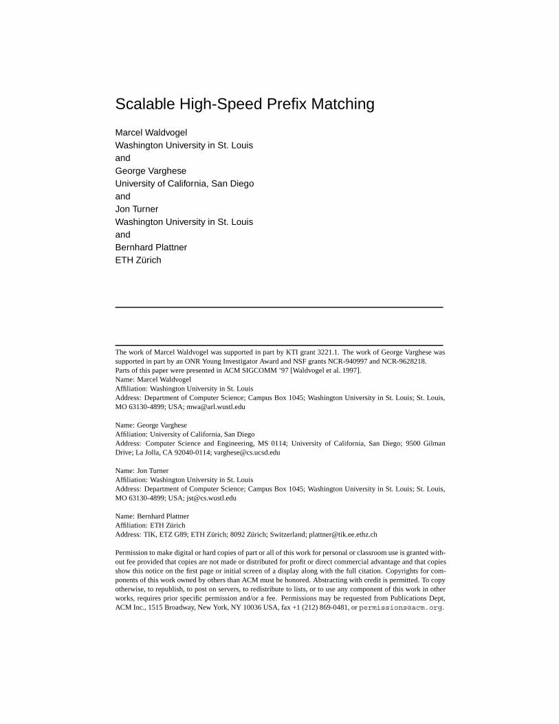
Fig. 1. Prefix Matching Overview
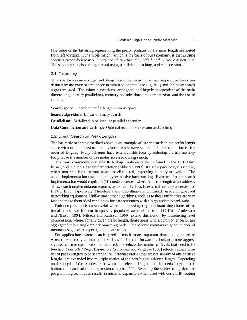
Traditionally, prefix matching has been done on tries [Gwehenberger 1968; Morrison1968], with bit-wise (binary) tries being the foremost representative. Figure 1 shows sucha trie. To find the longest prefix matching a given search string, the tree is traversed startingat the root (topmost) node. Depending on the value of the next bit in the search string, eitherthe left or right link is followed, always remembering the most recent prefix node visited.When the search string is exhausted or a nonexistent link is selected, the remembered prefixnode is returned as the best match.
Thus a trie has two aspects (Figure 1) that we base our taxonomy on: the first is thevertical aspect that signifies prefix length (as we travel vertically down the trie the prefixeswe encounter are correspondingly longer); the second horizontal aspect is the prefix value
Scalable High-Speed Prefix Matching · 5
(the value of the bit string representing the prefix, prefixes of the same length are sortedfrom left to right). Our simple insight, which is the basis of our taxonomy, is that existingschemes either do linear or binary search in either the prefix length or value dimensions.The schemes can also be augmented using parallelism, caching, and compression.
2.1 Taxonomy
Thus our taxonomy is organized along four dimensions. The two major dimensions aredefined by the main search space in which to operate (see Figure 1) and the basic searchalgorithm used. The minor dimensions, orthogonal and largely independent of the maindimensions, identify parallelism, memory optimizations and compression, and the use ofcaching.
Search space: Search in prefix length or value space
Search algorithm: Linear or binary search
Parallelism: Serialized, pipelined, or parallel execution
Data Compaction and caching: Optional use of compression and caching.
2.2 Linear Search on Prefix Lengths
The basic trie scheme described above is an example of linear search in the prefix lengthspace without compression. This is because trie traversal explores prefixes in increasingorder of lengths. Many schemes have extended this idea by reducing the trie memoryfootprint or the number of trie nodes accessed during search.
The most commonly available IP lookup implementation is found in the BSD Unixkernel, and is a radix trie implementation [Sklower 1993]. It uses a path-compressed trie,where non-branching internal nodes are eliminated, improving memory utilization. Theactual implementation uses potentially expensive backtracking. Even an efficient searchimplementation would require O(W ) node accesses, where W is the length of an address.Thus, search implementation requires up to 32 or 128 costly external memory accesses, forIPv4 or IPv6, respectively. Therefore, these algorithms are not directly used in high-speednetworking equipment. Unlike most other algorithms, updates to these unibit tries are veryfast and make them ideal candidates for data structures with a high update/search ratio.
Path compression is most useful when compressing long non-branching chains of in-ternal nodes, which occur in sparsely populated areas of the trie. LC-Tries [Anderssonand Nilsson 1994; Nilsson and Karlsson 1999] extend this notion by introducing levelcompression, where, for any given prefix length, dense areas with a common ancestor areaggregated into a single 2k-ary branching node. This scheme maintains a good balance ofmemory usage, search speed, and update times.
For applications where search speed is much more important than update speed orworst-case memory consumption, such as for Internet forwarding lookups, more aggres-sive search time optimization is required. To reduce the number of levels that need to betouched, Controlled Prefix Expansion [Srinivasan and Varghese 1999] selects a small num-ber of prefix lengths to be searched. All database entries that are not already of one of theselengths, are expanded into multiple entries of the next higher selected length. Dependingon the length of the “strides” s between the selected lengths and the prefix length distri-bution, this can lead to an expansion of up to 2s−1. Selecting the strides using dynamicprogramming techniques results in minimal expansion when used with current IP routing
6 · M. Waldvogel, G. Varghese, J. Turner, and B. Plattner
tables. Despite expansion, this search scheme is still linear in the prefix length becauseexpansion only provides a constant factor improvement.
Prefix expansion is used generously in the scheme developed by Gupta et al. [Guptaet al. 1998] to reduce memory accesses even further. In the DIR-24-8 scheme presentedthere, all prefixes are expanded to at least 24 bits (the Internet backbone forwarding tablescontain almost no prefixes longer than 24 bits). A typical lookup will then just use the mostsignificant 24 bits of the address as an index into the 16M entries of the table, reducing theexpected number of memory accesses to almost one.
A different approach was chosen by Degermark et al. [Degermark et al. 1997]. By firstexpanding to a complete trie and then using bit vectors and mapping tables, they are ableto represent routing tables of up to 40,000 entries in around 150KBytes. This compactrepresentation allows the data to be kept in on-chip caches, which provide much betterperformance than standard off-chip memory. A further approach to trie compression usingbitmaps is described in [Eatherton 1999].
Crescenzi et al. [Crescenzi et al. 1999] present another compressed trie lookup scheme.They first fully expand the trie, so that all leaf nodes are at length W . Then, they dividethe tree into multiple subtrees of identical size. These slices are then put side-by-side, say,in columns. All the neighboring identical rows are then collapsed, and a single table iscreated to map from the original row number to the new, compressed row number. Unlikethe previous approach [Degermark et al. 1997], this does not result in a small enough tableto fit into typical on-chip caches, yet it guarantees that all lookups can be done in exactly3 indexed memory lookups.
McAuley and Francis [McAuley and Francis 1993] use standard (“binary”) content-addressable memories (CAMs) to quickly search the different prefix lengths. The firstsolution discussed requires multiple passes through, starting with the longest prefix. Thissearch order was chosen to be able to terminate after the first match. The other solutionis to have multiple CAMs queried in parallel. CAMs are generally much slower than con-ventional memory and do not provide enough entries for backbone routers are still rare,where in the near future more than 100,000 forwarding entries will be required. Never-theless, CAMs are popular in edge routers, which typically only have up to hundreds offorwarding entries.
2.3 Binary Search on Prefix Lengths
The prior work closest to binary search on prefix lengths occurs in computational geometry.De Berg et al. [de Berg et al. 1995] describe a scheme for one-dimensional point locationbased on stratified trees [van Emde Boas 1975; van Emde Boas et al. 1977]. A stratifiedtree is probably best described as a self-similar tree, where each node internally has thesame structure as the overall tree. The actual search is not performed on a prefix trie, buton a balanced interval tree. The scheme does not support overlapping regions, which arerequired to implement prefix lookups. While this could be resolved in a preprocessingstep, it would degrade the incremental update time to O(N). Also unlike the algorithmintroduced in Section 3, it cannot take advantage of additional structure in the routing table(Section 4).
2.4 Linear Search of Values
Pure linear value search is only reasonable for very small tables. But a hardware-parallelversion using ternary CAMs has become attractive in the recent years. Ternary CAMs,
Scalable High-Speed Prefix Matching · 7
unlike the binary CAMs above, which require multiple stages or multiple CAMs, have amask associated with every entry. This mask is used to describe which bits of the entryshould be compared to the query key, allowing for one-pass prefix matching. Due to thehigher per-entry hardware overhead, ternary CAMs typically provide for only about halfthe entries as comparable binary CAMs. Also, as multiple entries may match for a singlesearch key, it becomes necessary to prioritize entries. As priorities are typically associ-ated with an internal memory address, inserting a new entry can potentially cause a largenumber of other entries to be shifted around. Shah and Gupta [Shah and Gupta 2000]present an algorithmic solution to minimize these shifts while Kobayashi et al. [Kobayashiet al. 2000] modify the CAM itself to return only the longest match with little hardwareoverhead.
2.5 Binary Search of Values
The use of binary search on the value space was originally proposed by Butler Lampsonand described in [Perlman 1992]; additional improvements were proposed in [Lampsonet al. 1998]. The key ideas are to represent each prefix as a range using two values (thelowest and highest values in the range), to preprocess the table to associate matching pre-fixes with these values, and then to do ordinary binary search on these values. The resultingsearch time is �log2 2N� search steps, with N being the number of routing table entries.With current routing table sizes, this gets close to the expected number of memory accessesfor unibit tries, which is fairly slow. However, lookup time can be reduced using B-treesinstead of binary trees and by using an initial memory lookup [Lampson et al. 1998].
2.6 Parallelism, Data Compaction, and Caches
The minor dimensions described above in our taxonomy can be applied to all the majorschemes. Almost every lookup algorithm can be pipelined. Also, almost all algorithmslend themselves to more compressed representations of their data structures; however, in[Degermark et al. 1997; Crescenzi et al. 1999; Eatherton 1999], the main novelty is themanner in which a multibit trie is compressed while retaining fast lookup times.
In addition, all of the lookup schemes can take advantage of an added lookup cache,which does not store the prefixes matched, but instead stores recent lookup keys, as exactmatches are generally much simpler and faster to implement. Unfortunately, with thegrowth of the Internet, access locality in packet streams seems to decrease, requiring largerand larger caches to achieve similar hit rates. In 1987, Feldmeier [Feldmeier 1988] foundthat a cache for the most recent 9 destination addresses already provided for a 90% hit rate.8 years later, Partridge [Partridge 1996] did a similar study, where caches with close to5000 entries were required to achieve the same hit rate. We expect this trend to continueand potentially to become even more pronounced.
2.7 Protocol Based Solutions
Finally, (leaving behind our taxonomy) we note that one way to finesse the problems of IPlookup is to have extra information sent along with the packet to simplify or even totallyget rid of IP lookups at routers. Two major proposals along these lines were IP Switching[Newman et al. 1997] and Tag Switching [Rekhter et al. 1997], both now mostly replacedby Multi-Protocol Label Switching (MPLS [Rosen et al. 2001]. All three schemes requirelarge, contiguous parts of the network to adopt their protocol changes before they willshow a major improvement. The speedup is achieved by adding information on the des-

8 · M. Waldvogel, G. Varghese, J. Turner, and B. Plattner
tination to every IP packet, a technique first described by Chandranmenon and Varghese[Chandranmenon and Varghese 1995]. This switching information is included by adding a“label” to each packet, a small integer that allows direct lookup in the router’s forwardingtable.
Neither scheme can completely avoid ordinary IP lookups. All schemes require theingress router (to the portions of the network implementing their protocol) to perform a fullrouting decision. In their basic form, both systems potentially require the boundary routersbetween autonomous systems (e.g., between a company and its ISP or between ISPs) toperform the full forwarding decision again, because of trust issues, scarce resources, ordifferent views of the network. Labels will become scarce resources, of which only a finiteamount exist. Thus towards the backbone, they need to be aggregated; away from thebackbone, they need to be separated again.
2.8 Summary of Existing Work
There are two basic solutions for the prefix matching problem caused by Internet growth:(1) making lookups faster or (2) reducing the number of lookups using caching or protocolmodifications. As seen above, the latter mechanisms are not able to completely avoidlookups, but only reduce them to either fewer routers (label switching) or fewer per router(caching). The advantage of using caches will disappear in a few years, as Internet datarates are growing much faster than hardware speeds, to the point that all lookup memorywill have to use the fastest available memory (i.e., SRAM of the kind that is currently usedby cache memory).
The most popularly deployed schemes today are based on linear search of prefix lengthsusing multibit or unibit tries together with high speed memories and pipelining. However,these algorithms do not scale well to longer next generation IP addresses. Lookup schemesbased on unibit tries and binary search are (currently) too slow and do not scale well; CAMsolutions are relatively expensive and are hard to field upgrade;
In summary, all existing schemes have problems of either performance, scalability, gen-erality, or cost, especially when addresses extend beyond the current 32 bits. We nowdescribe a lookup scheme that has good performance, is scalable to large addresses, anddoes not require protocol changes. Our scheme allows a cheap, fast software implementa-tion, and is also amenable to hardware implementations.
3. BASIC BINARY SEARCH SCHEME
Our basic algorithm is based on three significant ideas: First, we use hashing to checkwhether an address D matches any prefix of a particular length; second, we use binarysearch to reduce number of searches from linear to logarithmic; third, we use pre-computationto prevent backtracking in case of failures in the binary search of a range. Rather thanpresent the final solution directly, we will gradually refine these ideas in Section 3.1, Sec-tion 3.2, and Section 3.4 to arrive at a working basic scheme. We describe further opti-mizations to the basic scheme in the next section. As there are multiple ways to look at thedata structure, whenever possible we will use the terms “shorter” and “longer” to signifyselecting shorter or longer prefixes.
3.1 Linear Search of Hash Tables
Our point of departure is a simple scheme that does linear search of hash tables organizedby prefix lengths. We will improve this scheme shortly to do binary search on the hash
Scalable High-Speed Prefix Matching · 9
tables.
Length Hash
5
7
12
01010
01010110110110
011011010101
Hash tables
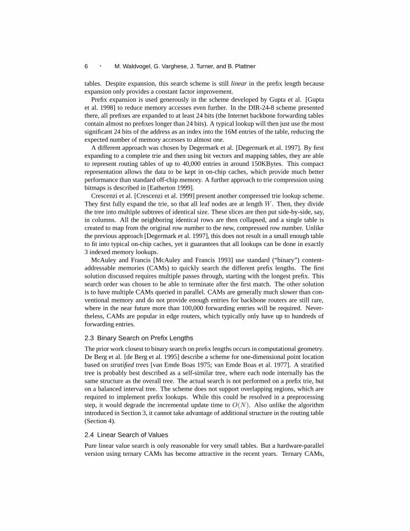
Fig. 2. Hash Tables for each possible prefix length
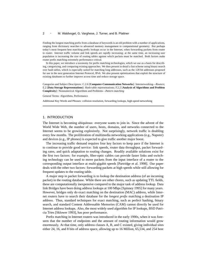
The idea is to look for all prefixes of a certain length l using hashing and use multiplehashes to find the best matching prefix, starting with the largest value of l and workingbackwards. Thus we start by dividing the database of prefixes according to lengths. As-suming a particularly tiny routing table with four prefixes of length 5, 7, 7, and 12, respec-tively, each of them would be stored in the hash table for its length (Figure 2). So eachset of prefixes of distinct length is organized as a hash table. If we have a sorted array Lcorresponding to the distinct lengths, we only have 3 entries in the array, with a pointer tothe longest length hash table in the last entry of the array.
To search for destination address D, we simply start with the longest length hash table l(i.e. 12 in the example), and extract the first l bits of D and do a search in the hash tablefor length l entries. If we succeed, we have found the longest match and thus our BMP; ifnot, we look at the first length smaller than l, say l ′ (this is easy to find if we have the arrayL by simply indexing one position less than the position of l), and continuing the search.
3.2 Binary Search of Hash Tables
The previous scheme essentially does (in the worst case) linear search among all dis-tinct string lengths. Linear search requires O(W ) time (more precisely, O(W dist), whereWdist ≤ W is the number of distinct lengths in the database.)
A better search strategy is to use binary search on the array L to cut down the numberof hashes to O(log Wdist). However, for binary search to make its branching decision, itrequires the result of an ordered comparison, returning whether the probed entry is “lessthan,” “equal,” or “greater than” our search key. As we are dealing with prefix lengths,these map to indications to look at “shorter,” “same length,” or “longer,” respectively.When dealing with hash lookups, ordered comparison does seem impossible: either thereis a hit (then the entry found equals the hash key) or there is a miss and thus no comparisonpossible.
Let’s look at the problem from the other side: In ordinary binary search, “equal” indi-cates that we have found the matching entry and can terminate the search. When searchingamong prefix lengths, having found a matching entry does not yet imply that this is also thebest entry. So clearly, when we have found a match, we need to continue searching amongthe longer prefixes. How does this observation help? It signifies, that when an entry hasbeen found, we should remember it as a potential candidate solution, but continue lookingfor longer prefixes. The only other information that we can get from the hash lookup is amiss. Due to limited choice, we start taking hash misses as an indication to inspect shorterprefixes. This results in the pseudo code given in Figure 3.
10 · M. Waldvogel, G. Varghese, J. Turner, and B. Plattner
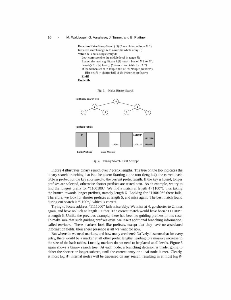
Function NaiveBinarySearch(D) (* search for address D *)Initialize search range R to cover the whole array L;While R is not a single entry do
Let i correspond to the middle level in range R;Extract the most significant L[i].length bits of D into D′;Search(D′, L[i].hash); (* search hash table for D′ *)If found then set R := longer half of R (*longer prefixes*)
Else set R := shorter half of R; (*shorter prefixes*)Endif
Endwhile
Fig. 3. Naıve Binary Search
(a) Binary search tree
1
2
3
4
6
5 7
0*
(b) Hash Tables
1111010
11001111100* 110011*
111100*
bold: Prefixes italic: Markers
Fig. 4. Binary Search: First Attempt
Figure 4 illustrates binary search over 7 prefix lengths. The tree on the top indicates thebinary search branching that is to be taken: Starting at the root (length 4), the current hashtable is probed for the key shortened to the current prefix length. If the key is found, longerprefixes are selected, otherwise shorter prefixes are tested next. As an example, we try tofind the longest prefix for “1100100.” We find a match at length 4 (1100*), thus takingthe branch towards longer prefixes, namely length 6. Looking for “110010*” there fails.Therefore, we look for shorter prefixes at length 5, and miss again. The best match foundduring our search is “1100*,” which is correct.
Trying to locate address “1111000” fails miserably: We miss at 4, go shorter to 2, missagain, and have no luck at length 1 either. The correct match would have been “111100*”at length 6. Unlike the previous example, there had been no guiding prefixes in this case.To make sure that such guiding prefixes exist, we insert additional branching information,called markers. These markers look like prefixes, except that they have no associatedinformation fields, their sheer presence is all we want for now.
But where do we need markers, and how many are there? Na ıvely, it seems that for everyentry, there would be a marker at all other prefix lengths, leading to a massive increase inthe size of the hash tables. Luckily, markers do not need to be placed at all levels. Figure 5again shows a binary search tree. At each node, a branching decision is made, going toeither the shorter or longer subtree, until the correct entry or a leaf node is met. Clearly,at most log W internal nodes will be traversed on any search, resulting in at most log W

Scalable High-Speed Prefix Matching · 11
branching decisions. Also, any search that will end up at a given node only has a singlepath to choose from, eliminating the need to place markers at any other levels.
(a) Binary search tree
1
2
3
4
6
5 7
0* 1111*
(b) Hash Tables including Markers
1111010
11001111100* 110011*
111100*
111101*
bold: Prefixes italic: Markers
Fig. 5. Improved Branching Decisions due to Markers
3.3 Problems with Backtracking
Unfortunately, the algorithm shown in Figure 3 is not correct as it stands and does not takelogarithmic time if fixed naıvely. The problem is that while markers are good things (theylead to potentially better, longer prefixes in the table), can also cause the search to followfalse leads which may fail. In case of failure, we would have to modify the binary search(for correctness) to backtrack and search the shorter prefixes of R again. Such a naıvemodification can lead us back to linear time search. An example will clarify this.
1
2
3
1*
00*
111*11*
Fig. 6. Misleading Markers
First consider the prefixes P1 = 1, P2 = 00, P3 = 111 (Figure 6). As discussed above,we add a marker to the middle table so that the middle hash table contains 00 (a real prefix)and 11 (a marker pointing down to P3). Now consider a search for 110. We start at themiddle hash table and get a hit; thus we search the third hash table for 110 and fail. But thecorrect best matching prefix is at the first level hash table — i.e., P1. The marker indicatingthat there will be longer prefixes, indispensable to find P3, was misleading in this case; soapparently, we have to go back and search the shorter half of the range.
The fact that each entry contributes at most log2 W markers may cause some readers tosuspect that the worst case with backtracking is limited to O(log2 W ). This is incorrect.The worst case is O(W ). The worst-case example for say W bits is as follows: we have a
12 · M. Waldvogel, G. Varghese, J. Turner, and B. Plattner
prefix Pi of length i, for 1 ≤ i < W that contains all 0s. In addition we have the prefix Qwhose first W − 1 bits are all zeroes, but whose last bit is a 1. If we search for the W bitaddress containing all zeroes then we can show that binary search with backtracking willtake O(W ) time and visit every level in the table. (The problem is that every level containsa false marker that indicates the presence of something better in the longer section.)
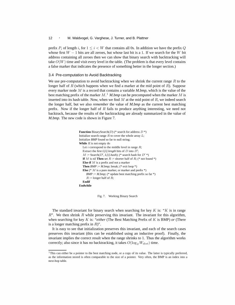
3.4 Pre-computation to Avoid Backtracking
We use pre-computation to avoid backtracking when we shrink the current range R to thelonger half of R (which happens when we find a marker at the mid point of R). Supposeevery marker node M is a record that contains a variable M.bmp, which is the value of thebest matching prefix of the marker M .1 M.bmp can be precomputed when the marker M isinserted into its hash table. Now, when we find M at the mid point of R, we indeed searchthe longer half, but we also remember the value of M.bmp as the current best matchingprefix. Now if the longer half of R fails to produce anything interesting, we need notbacktrack, because the results of the backtracking are already summarized in the value ofM.bmp. The new code is shown in Figure 7.
Function BinarySearch(D) (* search for address D *)Initialize search range R to cover the whole array L;Initialize BMP found so far to null string;While R is not empty do
Let i correspond to the middle level in range R;Extract the first L[i].length bits of D into D′;M := Search(D′, L[i].hash); (* search hash for D′ *)If M is nil Then set R := shorter half of R; (* not found *)Else-if M is a prefix and not a markerThen BMP := M.bmp; break; (* exit loop *)Else (* M is a pure marker, or marker and prefix *)
BMP := M.bmp; (* update best matching prefix so far *)R := longer half of R;
EndifEndwhile
Fig. 7. Working Binary Search
The standard invariant for binary search when searching for key K is: “K is in rangeR”. We then shrink R while preserving this invariant. The invariant for this algorithm,when searching for key K is: “either (The Best Matching Prefix of K is BMP) or (Thereis a longer matching prefix in R)”.
It is easy to see that initialization preserves this invariant, and each of the search casespreserves this invariant (this can be established using an inductive proof). Finally, theinvariant implies the correct result when the range shrinks to 1. Thus the algorithm workscorrectly; also since it has no backtracking, it takes O(log2 Wdist) time.
1This can either be a pointer to the best matching node, or a copy of its value. The latter is typically preferred,as the information stored is often comparable to the size of a pointer. Very often, the BMP is an index into anext-hop table.

Scalable High-Speed Prefix Matching · 13
4. REFINEMENTS TO BASIC SCHEME
The basic scheme described in Section 3 takes just 7 hash computations, in the worst case,for 128 bit IPv6 addresses. However, each hash computation takes at least one access tomemory; at gigabit speeds each memory access is significant. Thus, in this section, weexplore a series of optimizations that exploit the deeper structure inherent to the problemto reduce the average number of hash computations.
1
10
100
1000
10000
2 4 6 8 10 12 14 16 18 20 22 24 26 28 30 32
Cou
nt
Prefix Length
AADSMaeEast
MaeWestPAIX
PacBellMaeEast 1996
Fig. 8. Histogram of Backbone Prefix Length Distributions (log scale)
4.1 Asymmetric Binary Search
We first describe a series of simple-minded optimizations. Our main optimization, mutat-ing binary search, is described in the next section. A reader can safely skip to Section 4.2on a first reading.
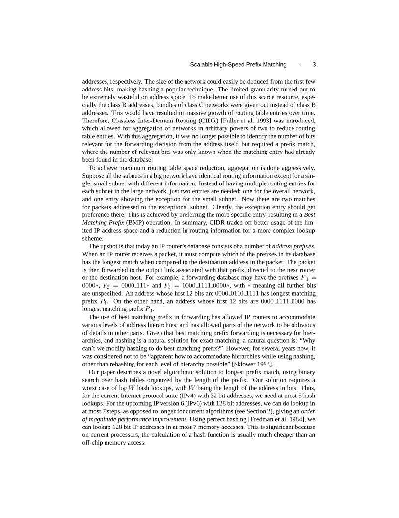
The current algorithm is a fast, yet very general, BMP search engine. Usually, theperformance of general algorithms can be improved by tailoring them to the particulardatasets they will be applied to. Figure 8 shows the prefix length distribution extractedfrom forwarding table snapshots from five major backbone sites in January 1999 and, forcomparison, at Mae-East in December 1996 2. As can be seen, the entries are distributedover the different prefix lengths in an extremely uneven fashion. The peak at length 24dominates everything by at least a factor of ten, if we ignore length 24. There are also morethan 100 times as many prefixes at length 24 than at any prefix outside the range 15 . . . 24.This graph clearly shows the remnants of the original class A, B, and C networks with localmaxima at lengths 8, 16, and 24. This distribution pattern is retained for many years nowand seems to be valid for all backbone routing tables, independent of their size (Mae-Easthas over 38,000, while PAIX has less than 6,000 entries).
These characteristics visibly cry for optimizations. Although we will quantify the po-tential improvements using these forwarding tables, we believe that the optimizations in-troduced below apply to any current or future set of addresses.
As the first improvement, which has already been mentioned and used in the basicscheme, the search can be limited to those prefix lengths which do contain at least one en-try, reducing the worst case number of hashes from log 2 W (5 with W = 32) to log2 Wdist
2http://www.merit.edu/ipma/routing table/
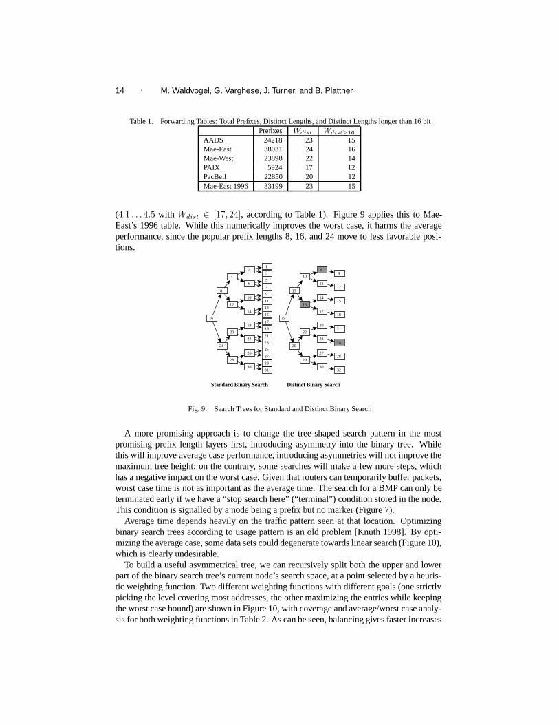
14 · M. Waldvogel, G. Varghese, J. Turner, and B. Plattner
Table 1. Forwarding Tables: Total Prefixes, Distinct Lengths, and Distinct Lengths longer than 16 bitPrefixes Wdist Wdist≥16
AADS 24218 23 15Mae-East 38031 24 16Mae-West 23898 22 14PAIX 5924 17 12PacBell 22850 20 12Mae-East 1996 33199 23 15
(4.1 . . . 4.5 with Wdist ∈ [17, 24], according to Table 1). Figure 9 applies this to Mae-East’s 1996 table. While this numerically improves the worst case, it harms the averageperformance, since the popular prefix lengths 8, 16, and 24 move to less favorable posi-tions.
31
29
27
25
23
21
19
17
15
13
11
9
7
5
3
1
30
26
22
18
14
10
6
2
28
20
12
4
24
16
8
32
28
24
21
18
15
12
9
30
27
23
20
17
14
11
8
29
22
16
10
26
19
13
Standard Binary Search Distinct Binary Search
Fig. 9. Search Trees for Standard and Distinct Binary Search
A more promising approach is to change the tree-shaped search pattern in the mostpromising prefix length layers first, introducing asymmetry into the binary tree. Whilethis will improve average case performance, introducing asymmetries will not improve themaximum tree height; on the contrary, some searches will make a few more steps, whichhas a negative impact on the worst case. Given that routers can temporarily buffer packets,worst case time is not as important as the average time. The search for a BMP can only beterminated early if we have a “stop search here” (“terminal”) condition stored in the node.This condition is signalled by a node being a prefix but no marker (Figure 7).
Average time depends heavily on the traffic pattern seen at that location. Optimizingbinary search trees according to usage pattern is an old problem [Knuth 1998]. By opti-mizing the average case, some data sets could degenerate towards linear search (Figure 10),which is clearly undesirable.
To build a useful asymmetrical tree, we can recursively split both the upper and lowerpart of the binary search tree’s current node’s search space, at a point selected by a heuris-tic weighting function. Two different weighting functions with different goals (one strictlypicking the level covering most addresses, the other maximizing the entries while keepingthe worst case bound) are shown in Figure 10, with coverage and average/worst case analy-sis for both weighting functions in Table 2. As can be seen, balancing gives faster increases
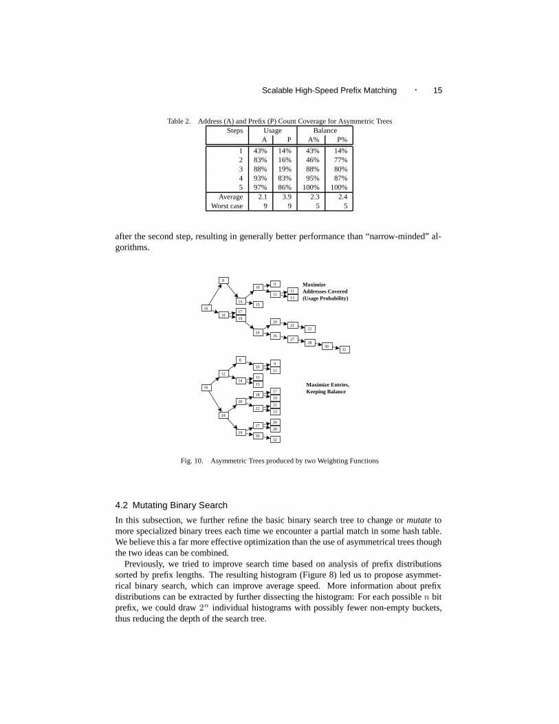
Scalable High-Speed Prefix Matching · 15
Table 2. Address (A) and Prefix (P) Count Coverage for Asymmetric TreesSteps Usage Balance
A P A% P%
1 43% 14% 43% 14%2 83% 16% 46% 77%3 88% 19% 88% 80%4 93% 83% 95% 87%5 97% 86% 100% 100%
Average 2.1 3.9 2.3 2.4Worst case 9 9 5 5
after the second step, resulting in generally better performance than “narrow-minded” al-gorithms.
26
20
12
9
24
15
10
19
17
14
18
16
8
13
11
2122
2728
3032
23
21
19
17
13
8
32
28
26
22
18
15
12
30
27
20
14
29
24
16
109
11
Maximize Entries,Keeping Balance
MaximizeAddresses Covered(Usage Probability)
Fig. 10. Asymmetric Trees produced by two Weighting Functions
4.2 Mutating Binary Search
In this subsection, we further refine the basic binary search tree to change or mutate tomore specialized binary trees each time we encounter a partial match in some hash table.We believe this a far more effective optimization than the use of asymmetrical trees thoughthe two ideas can be combined.
Previously, we tried to improve search time based on analysis of prefix distributionssorted by prefix lengths. The resulting histogram (Figure 8) led us to propose asymmet-rical binary search, which can improve average speed. More information about prefixdistributions can be extracted by further dissecting the histogram: For each possible n bitprefix, we could draw 2n individual histograms with possibly fewer non-empty buckets,thus reducing the depth of the search tree.
16 · M. Waldvogel, G. Varghese, J. Turner, and B. Plattner
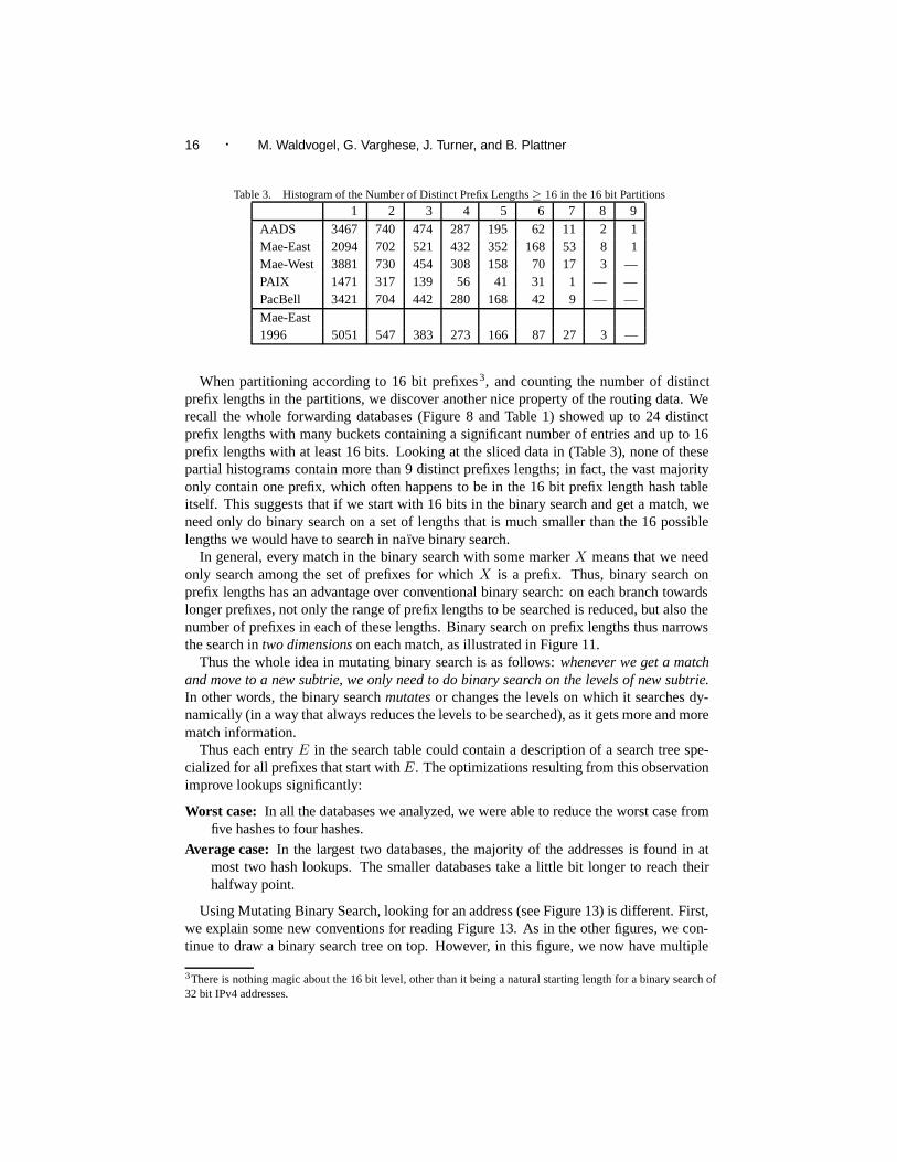
Table 3. Histogram of the Number of Distinct Prefix Lengths ≥ 16 in the 16 bit Partitions
1 2 3 4 5 6 7 8 9AADS 3467 740 474 287 195 62 11 2 1Mae-East 2094 702 521 432 352 168 53 8 1Mae-West 3881 730 454 308 158 70 17 3 —PAIX 1471 317 139 56 41 31 1 — —PacBell 3421 704 442 280 168 42 9 — —Mae-East1996 5051 547 383 273 166 87 27 3 —
When partitioning according to 16 bit prefixes3, and counting the number of distinctprefix lengths in the partitions, we discover another nice property of the routing data. Werecall the whole forwarding databases (Figure 8 and Table 1) showed up to 24 distinctprefix lengths with many buckets containing a significant number of entries and up to 16prefix lengths with at least 16 bits. Looking at the sliced data in (Table 3), none of thesepartial histograms contain more than 9 distinct prefixes lengths; in fact, the vast majorityonly contain one prefix, which often happens to be in the 16 bit prefix length hash tableitself. This suggests that if we start with 16 bits in the binary search and get a match, weneed only do binary search on a set of lengths that is much smaller than the 16 possiblelengths we would have to search in na ıve binary search.
In general, every match in the binary search with some marker X means that we needonly search among the set of prefixes for which X is a prefix. Thus, binary search onprefix lengths has an advantage over conventional binary search: on each branch towardslonger prefixes, not only the range of prefix lengths to be searched is reduced, but also thenumber of prefixes in each of these lengths. Binary search on prefix lengths thus narrowsthe search in two dimensions on each match, as illustrated in Figure 11.
Thus the whole idea in mutating binary search is as follows: whenever we get a matchand move to a new subtrie, we only need to do binary search on the levels of new subtrie.In other words, the binary search mutates or changes the levels on which it searches dy-namically (in a way that always reduces the levels to be searched), as it gets more and morematch information.
Thus each entry E in the search table could contain a description of a search tree spe-cialized for all prefixes that start with E. The optimizations resulting from this observationimprove lookups significantly:
Worst case: In all the databases we analyzed, we were able to reduce the worst case fromfive hashes to four hashes.
Average case: In the largest two databases, the majority of the addresses is found in atmost two hash lookups. The smaller databases take a little bit longer to reach theirhalfway point.
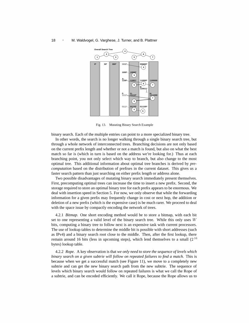
Using Mutating Binary Search, looking for an address (see Figure 13) is different. First,we explain some new conventions for reading Figure 13. As in the other figures, we con-tinue to draw a binary search tree on top. However, in this figure, we now have multiple
3There is nothing magic about the 16 bit level, other than it being a natural starting length for a binary search of32 bit IPv4 addresses.

Scalable High-Speed Prefix Matching · 17
X
Root
New Trie on Failure
m = Median Lengthamong all prefixlengths in trie
New Trie on Match(first m bits ofPrefix = X)
Fig. 11. Showing how mutating binary search for prefix P dynamically changes the trie on which it will dobinary search of hash tables.
0%
20%
40%
60%
80%
100%
1 2 3 4
Pref
ixes
fou
nd
Search Steps
AADSMaeEast
MaeWestPAIX
PacBellMaeEast 1996
Average
Fig. 12. Number of Hash Lookups (Note: No average-case optimizations)
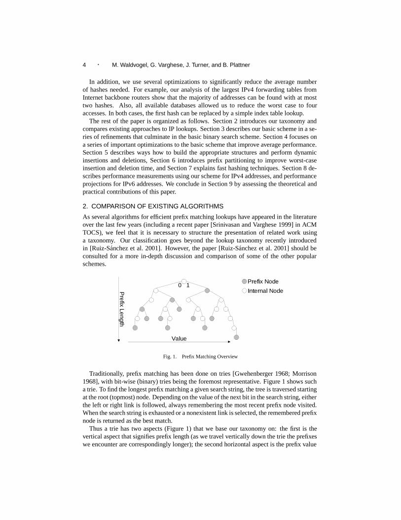
partial trees, originating from any prefix entry. This is because the search process willmove from tree to tree, starting with overall tree. Each binary tree has the “root” level (i.e.,the first length to be searched) at the left; the left child of each binary tree node is the lengthto be searched on failure, and whenever there is a match, the search switches to the morespecific tree.
Consider now a search for address 1100110, matching the prefix labelled B, in thedatabase of Figure 13. The search starts with the generic tree, so length 4 is checked,finding A. Among the prefixes starting with A, there are known to be only three distinctlengths (4, 5, and 6). So A contains a description of the new tree, limiting the searchappropriately. This tree is drawn as rooting in A. Using this tree, we find B, giving a newtree, the empty tree. The binary tree has mutated from the original tree of 7 lengths, to asecondary tree of 3 lengths, to a tertiary empty “tree”.
Looking for 1111011, matching G, is similar. Using the overall tree, we find F . Switch-ing to its tree, we miss at length 7. Since a miss (no entry found) can’t update a tree, wefollow our current tree upwards to length 5, where we find G.
In general, whenever we go down in the current tree, we can potentially move to aspecialized binary tree because each match in the binary search is longer than any previousmatches, and hence may contain more specialized information. Mutating binary trees arisenaturally in our application (unlike classical binary search) because each level in the binarysearch has multiple entries stored in a hash table. as opposed to a single entry in classical
18 · M. Waldvogel, G. Varghese, J. Turner, and B. Plattner
1
2
3
4
6
5 7
Overall Search Tree
0* 00* 000*
10000*1000*
0000* 000000*
1111* 11110* 1111000
6
5
5
7
1100* 11001* 110000* 1100000
65 7
110011*B:
A:
F: G: H:
0111* 01110* 011100*5
6
Fig. 13. Mutating Binary Search Example
binary search. Each of the multiple entries can point to a more specialized binary tree.In other words, the search is no longer walking through a single binary search tree, but
through a whole network of interconnected trees. Branching decisions are not only basedon the current prefix length and whether or not a match is found, but also on what the bestmatch so far is (which in turn is based on the address we’re looking for.) Thus at eachbranching point, you not only select which way to branch, but also change to the mostoptimal tree. This additional information about optimal tree branches is derived by pre-computation based on the distribution of prefixes in the current dataset. This gives us afaster search pattern than just searching on either prefix length or address alone.
Two possible disadvantages of mutating binary search immediately present themselves.First, precomputing optimal trees can increase the time to insert a new prefix. Second, thestorage required to store an optimal binary tree for each prefix appears to be enormous. Wedeal with insertion speed in Section 5. For now, we only observe that while the forwardinginformation for a given prefix may frequently change in cost or next hop, the addition ordeletion of a new prefix (which is the expensive case) is be much rarer. We proceed to dealwith the space issue by compactly encoding the network of trees.
4.2.1 Bitmap. One short encoding method would be to store a bitmap, with each bitset to one representing a valid level of the binary search tree. While this only uses Wbits, computing a binary tree to follow next is an expensive task with current processors.The use of lookup tables to determine the middle bit is possible with short addresses (suchas IPv4) and a binary search root close to the middle. Then, after the first lookup, thereremain around 16 bits (less in upcoming steps), which lend themselves to a small (2 16
bytes) lookup table.
4.2.2 Rope. A key observation is that we only need to store the sequence of levels whichbinary search on a given subtrie will follow on repeated failures to find a match. This isbecause when we get a successful match (see Figure 11), we move to a completely newsubtrie and can get the new binary search path from the new subtrie. The sequence oflevels which binary search would follow on repeated failures is what we call the Rope ofa subtrie, and can be encoded efficiently. We call it Rope, because the Rope allows us to

Scalable High-Speed Prefix Matching · 19
swing from tree to tree in our network of interconnected binary search trees.If we consider a binary search tree, we define the Rope for the root of the trie node to
be the sequence of trie levels we will consider when doing binary search on the trie levelswhile failing at every point. This is illustrated in Figure 14. In doing binary search we startat Level m which is the median length of the trie. If we fail, we try at the quartile length(say n), and if we fail at n we try at the one-eight level (say o), and so on. The sequencem,n, o, . . . is the Rope for the trie.
m
n
o Eight Level
Quarter Level
Median Level
m
n
o
•
• • •
Fig. 14. In terms of a trie, a rope for the trie node is the sequence of lengths starting from the median length, thequartile length, and so on, which is the same as the series of left children (see dotted oval in binary tree on right)of a perfectly balanced binary tree on the trie levels.
Figure 15 shows the Ropes containing the same information as the trees in Figure 13.Note that a Rope can be stored using only log2 W (7 for IPv6) pointers. Since each pointerneeds to only discriminate among at most W possible levels, each pointer requires onlylog2 W bits. For IPv6, 64 bits of Rope is more than sufficient, though it seems possibleto get away with 32 bits of Rope in most practical cases. Thus a Rope is usually notlonger than the storage required to store a pointer. To minimize storage in the forwardingdatabase, a single bit can be used to decide whether the rope or only a pointer to a rope isstored in a node.
1
2
4Initial Rope
0* 00* 000*
10000*1000*
0000* 000000*
1111* 11110* 1111000
6
5
5
7
1100* 11001* 110000* 1100000
65
7
110011*
0111* 01110* 011100*5 6
3
Fig. 15. Sample Ropes
20 · M. Waldvogel, G. Varghese, J. Turner, and B. Plattner
Using the Rope as the data structure has a second advantage: it simplifies the algorithm.A Rope can easily be followed, by just picking pointer after pointer in the Rope, until thenext hit. Each strand in the Rope is followed in turn, until there is a hit (which starts a newRope), or the end of the Rope is reached. Following the Rope on processors is easily doneusing “shift right” instructions.
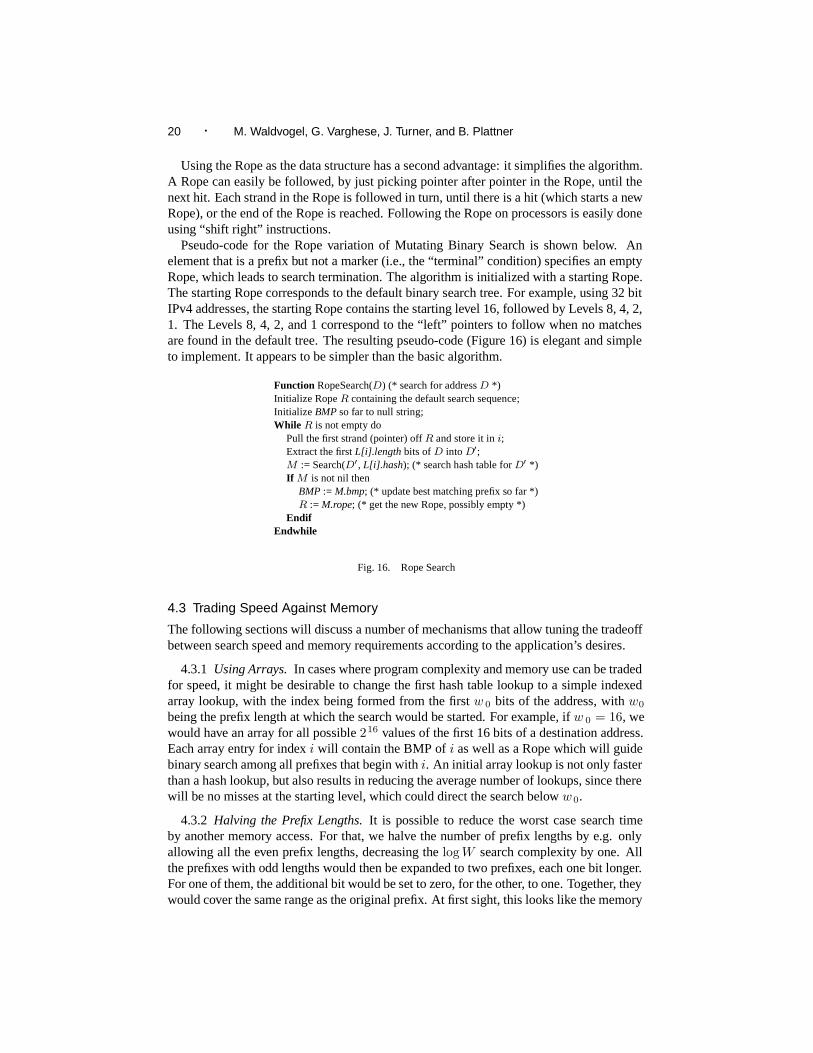
Pseudo-code for the Rope variation of Mutating Binary Search is shown below. Anelement that is a prefix but not a marker (i.e., the “terminal” condition) specifies an emptyRope, which leads to search termination. The algorithm is initialized with a starting Rope.The starting Rope corresponds to the default binary search tree. For example, using 32 bitIPv4 addresses, the starting Rope contains the starting level 16, followed by Levels 8, 4, 2,1. The Levels 8, 4, 2, and 1 correspond to the “left” pointers to follow when no matchesare found in the default tree. The resulting pseudo-code (Figure 16) is elegant and simpleto implement. It appears to be simpler than the basic algorithm.
Function RopeSearch(D) (* search for address D *)Initialize Rope R containing the default search sequence;Initialize BMP so far to null string;While R is not empty do
Pull the first strand (pointer) off R and store it in i;Extract the first L[i].length bits of D into D′;M := Search(D′, L[i].hash); (* search hash table for D′ *)If M is not nil then
BMP := M.bmp; (* update best matching prefix so far *)R := M.rope; (* get the new Rope, possibly empty *)
EndifEndwhile
Fig. 16. Rope Search
4.3 Trading Speed Against Memory
The following sections will discuss a number of mechanisms that allow tuning the tradeoffbetween search speed and memory requirements according to the application’s desires.
4.3.1 Using Arrays. In cases where program complexity and memory use can be tradedfor speed, it might be desirable to change the first hash table lookup to a simple indexedarray lookup, with the index being formed from the first w 0 bits of the address, with w0
being the prefix length at which the search would be started. For example, if w 0 = 16, wewould have an array for all possible 216 values of the first 16 bits of a destination address.Each array entry for index i will contain the BMP of i as well as a Rope which will guidebinary search among all prefixes that begin with i. An initial array lookup is not only fasterthan a hash lookup, but also results in reducing the average number of lookups, since therewill be no misses at the starting level, which could direct the search below w0.
4.3.2 Halving the Prefix Lengths. It is possible to reduce the worst case search timeby another memory access. For that, we halve the number of prefix lengths by e.g. onlyallowing all the even prefix lengths, decreasing the log W search complexity by one. Allthe prefixes with odd lengths would then be expanded to two prefixes, each one bit longer.For one of them, the additional bit would be set to zero, for the other, to one. Together, theywould cover the same range as the original prefix. At first sight, this looks like the memory

Scalable High-Speed Prefix Matching · 21
requirement will be doubled. It can be shown that the worst case memory consumption isnot affected, since the number of markers is reduced at the same time.
With W bits length, each entry could possibly require up to log(W ) − 1 markers (theentry itself is the log W th entry). When expanding prefixes as described above, some of theprefixes will be doubled. At the same time, W is halved, thus each of the prefixes requiresat most log(W/2) − 1 = log(W ) − 2 markers. Since they match in all but their least bit,they will share all the markers, resulting again in at most log W entries in the hash tables.
A second halving of the number of prefixes again decreases the worst case search time,but this time increases the amount of memory, since each prefix can be extended by up totwo bits, resulting in four entries to be stored, expanding the maximum number of entriesneeded per prefix to log(W ) + 1. For many cases the search speed improvement willwarrant the small increase in memory.
4.3.3 Internal Caching. Figure 8 showed that the prefixes with lengths 8, 16, and 24cover most of the address space used. Using binary search, these three lengths can becovered in just two memory accesses. To speed up the search, each address that requiresmore than two memory accesses to search for will be cached in one of these address lengthsaccording to Figure 17. Compared to traditional caching of complete addresses, thesecache prefixes cover a larger area and thus allow for a better utilization.
Function CacheInternally(A, P , L, M )(* found prefix P at length L after taking M memory accesses
searching for A *)If M > 2 then (* Caching can be of advantage *)
Round up prefix length L to next multiple of 8;Insert copy of P ’s entry at L, using the L first bits of A;
Endif
Fig. 17. Building the Internal Cache
4.4 Very Long Addresses
All the calculations above assume the processor’s registers are big enough to hold entireaddresses. For long addresses, such as those used for IP version 6, this does not alwayshold. We define w as the number of bits the registers hold. Instead of working on the entireaddress at once, the database is set up similar to a multibit trie [Srinivasan and Varghese1999] of stride w, resulting in a depth of k := W/w. Each of these “trie nodes” is thenimplemented using binary search. If the “trie nodes” used conventional technology, eachof them would require O(2w) memory, clearly impractical with modern processors, whichmanipulate 32 or 64 bits at a time.
Slicing the database into chunks of w bits also requires less storage than unsliced databases,since not the entire long addresses do not need to be stored with every element. The smallerfootprint of an entry also helps with hash collisions (Section 7).
This storage advantage comes at a premium: Slower access. The number of memoryaccesses changes from log2 W to k + log2 w, if the search in the intermediate “trie nodes”begins at their maximum length. This has no impact on IPv6 searches on modern 64 bitprocessors (Alpha, UltraSparc, Merced), which stay at 7 accesses. For 32 bit processors,the worst case using the basic scheme raises by 1, to 8 accesses.
22 · M. Waldvogel, G. Varghese, J. Turner, and B. Plattner
4.5 Hardware Implementations
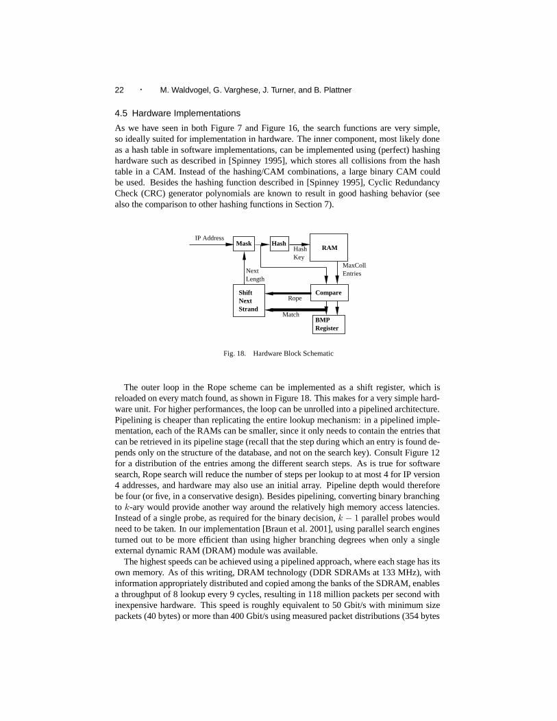
As we have seen in both Figure 7 and Figure 16, the search functions are very simple,so ideally suited for implementation in hardware. The inner component, most likely doneas a hash table in software implementations, can be implemented using (perfect) hashinghardware such as described in [Spinney 1995], which stores all collisions from the hashtable in a CAM. Instead of the hashing/CAM combinations, a large binary CAM couldbe used. Besides the hashing function described in [Spinney 1995], Cyclic RedundancyCheck (CRC) generator polynomials are known to result in good hashing behavior (seealso the comparison to other hashing functions in Section 7).
RAMMask
ShiftNextStrand
Compare
IP Address
HashKey
Rope
Match
NextLength
BMPRegister
Hash
MaxCollEntries
Fig. 18. Hardware Block Schematic
The outer loop in the Rope scheme can be implemented as a shift register, which isreloaded on every match found, as shown in Figure 18. This makes for a very simple hard-ware unit. For higher performances, the loop can be unrolled into a pipelined architecture.Pipelining is cheaper than replicating the entire lookup mechanism: in a pipelined imple-mentation, each of the RAMs can be smaller, since it only needs to contain the entries thatcan be retrieved in its pipeline stage (recall that the step during which an entry is found de-pends only on the structure of the database, and not on the search key). Consult Figure 12for a distribution of the entries among the different search steps. As is true for softwaresearch, Rope search will reduce the number of steps per lookup to at most 4 for IP version4 addresses, and hardware may also use an initial array. Pipeline depth would thereforebe four (or five, in a conservative design). Besides pipelining, converting binary branchingto k-ary would provide another way around the relatively high memory access latencies.Instead of a single probe, as required for the binary decision, k − 1 parallel probes wouldneed to be taken. In our implementation [Braun et al. 2001], using parallel search enginesturned out to be more efficient than using higher branching degrees when only a singleexternal dynamic RAM (DRAM) module was available.
The highest speeds can be achieved using a pipelined approach, where each stage has itsown memory. As of this writing, DRAM technology (DDR SDRAMs at 133 MHz), withinformation appropriately distributed and copied among the banks of the SDRAM, enablesa throughput of 8 lookup every 9 cycles, resulting in 118 million packets per second withinexpensive hardware. This speed is roughly equivalent to 50 Gbit/s with minimum sizepackets (40 bytes) or more than 400 Gbit/s using measured packet distributions (354 bytes
Scalable High-Speed Prefix Matching · 23
average) from June 1997.4 Using custom hardware and pipelining, we thus expect a sig-nificant speedup to software performance, allowing for affordable IP forwarding reachingfar beyond the single-device transmission speeds currently reached in high-tech researchlabs.
5. BUILDING AND UPDATING
Besides hashing and binary search, a predominant idea in this paper is pre-computation.Every hash table entry has an associated bmp field and (possibly) a Rope field, both ofwhich are precomputed. Pre-computation allows fast search but requires more complexInsertion routines. However, as mentioned earlier, while the routes stored with the prefixesmay change frequently, the addition of a new prefix (the expensive case) is much rarer.Thus it is worth paying a penalty for Insertion in return for improved search speed.
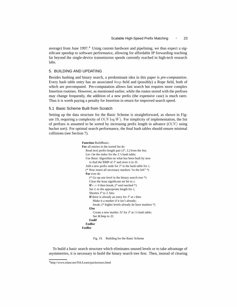
5.1 Basic Scheme Built from Scratch
Setting up the data structure for the Basic Scheme is straightforward, as shown in Fig-ure 19, requiring a complexity of O(N log W ). For simplicity of implementation, the listof prefixes is assumed to be sorted by increasing prefix length in advance (O(N) usingbucket sort). For optimal search performance, the final hash tables should ensure minimalcollisions (see Section 7).
Function BuildBasic;For all entries in the sorted list do
Read next prefix-length pair (P , L) from the list;Let i be the index for the L’s hash table;Use Basic Algorithm on what has been built by now
to find the BMP of P and store it in B;Add a new prefix node for P in the hash table for i;(* Now insert all necessary markers “to the left” *)For ever do
(* Go up one level in the binary search tree *)Clear the least significant set bit in i;If i = 0 then break; (* end reached *)Set L to the appropriate length for i;Shorten P to L bits;If there is already an entry for P at i then
Make it a marker if it isn’t already;break; (* higher levels already do have markers *)
ElseCreate a new marker M for P at i’s hash table;Set M.bmp to B;
EndifEndfor
Endfor
Fig. 19. Building for the Basic Scheme
To build a basic search structure which eliminates unused levels or to take advantage ofasymmetries, it is necessary to build the binary search tree first. Then, instead of clearing
4http://www.nlanr.net/NA/Learn/packetsizes.html
24 · M. Waldvogel, G. Varghese, J. Turner, and B. Plattner
the least significant bit, as outlined in Figure 19, the build algorithm really has to followthe binary search tree back up to find the “parent” prefix length. Some of these parentsmay be at longer prefix lengths, as illustrated in Figure 5. Since markers only need to beset at shorter prefix lengths, any parent associated with longer prefixes is just ignored.
5.2 Rope Search from Scratch
There are two ways to build the data structure suitable for Rope Search:
Simple: The search order does not divert from the overall binary search tree, only missinglevels are left out. This results in only minor improvements on the search speed andcan be implemented as a straightforward enhancement to Figure 19.
Optimal: Calculating the shortest Ropes on all branching levels requires the solution toan optimization problem in two dimensions. As we have seen, each branch towardslonger prefix lengths also limits the set of remaining prefixes.
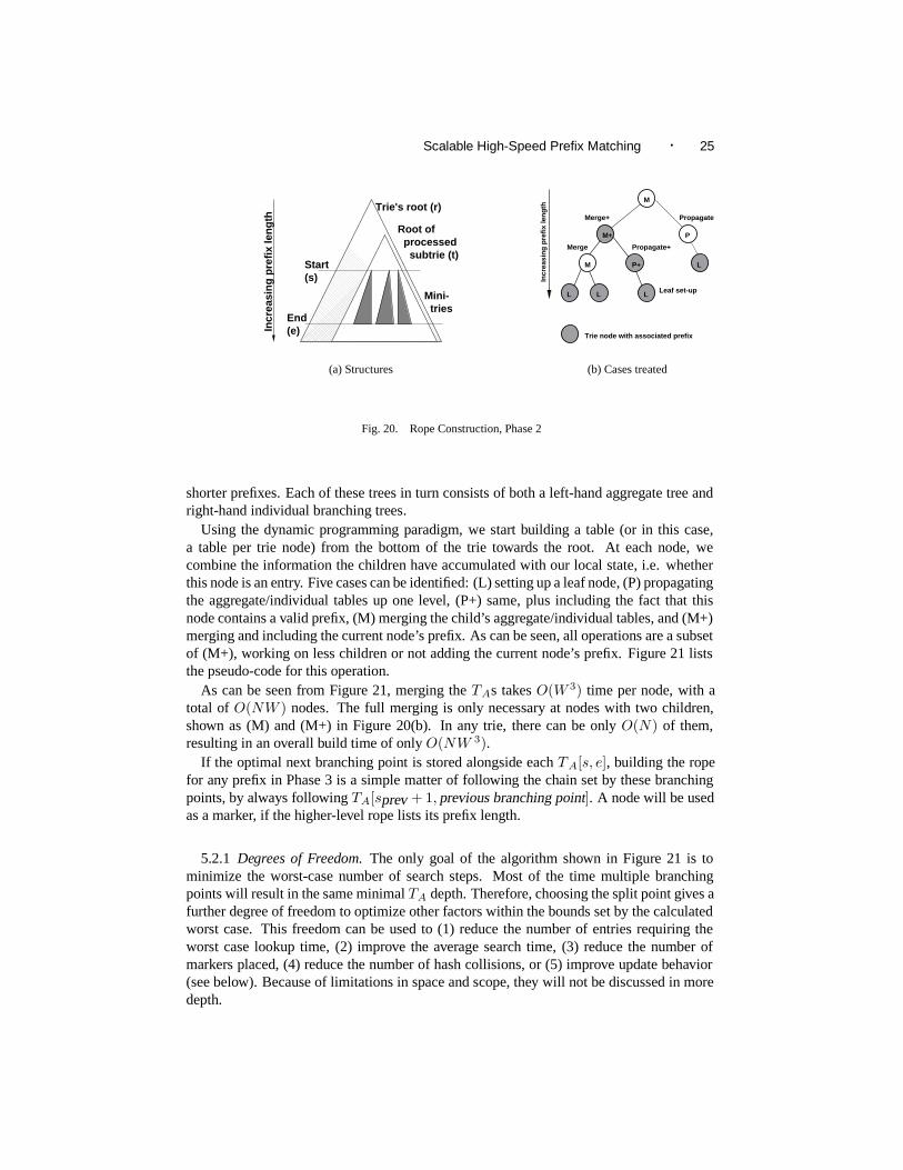
We present the algorithm which globally calculates the minimum Ropes, based on dynamicprogramming. The algorithm can be split up into three main phases:
(1) Build a conventional (uncompressed) trie structure with O(NW ) nodes containing allthe prefixes (O(NW ) time and space).
(2) Walk through the trie bottom-up, calculating the cost of selecting different branchingpoints and combining them on the way up using dynamic programming (O(NW 3)time and space).
(3) Walk through the trie top-down, build the Ropes using the results from phase 2, andinsert the entries into the hash tables (O(NW log W ) time, working on the spaceallocated in phase 2).
To understand the bottom-up merging of the information in phase 2, let us first look atthe information that is necessary for bottom-up merging. Recall the Ropes in Figure 15. Ateach branching point, the search either turns towards longer prefixes and a more specificbranching tree, or towards shorter prefixes without changing the set of levels. The goal isto minimize worst-case search cost, or the number of hash lookups required. The overallcost of putting a decision point at prefix length x is the maximum path length on either sideplus one for the newly inserted decision. Looking at Figure 15, the longest path on the leftof our starting point has length two (the paths to 0∗ or 000∗). When looking at the righthand side, the longest of the individual searches require two lookups (11001∗, 1100000,11110∗, and 0111000).
Generalizing, for each range R covered and each possible prefix length x splitting thisrange into two halves, Rl and Rr, the program needs to calculate the maximum depthof the aggregate left-hand tree R l, covering shorter prefixes, and the maximum depth ofthe individual right-hand trees Rr. When trying to find an optimal solution, the goal isto minimize these maxima, of course. Clearly, this process can be applied recursively.Instead of implementing a simple-minded recursive algorithm in exponential time, we usedynamic programming to solve it in polynomial time.
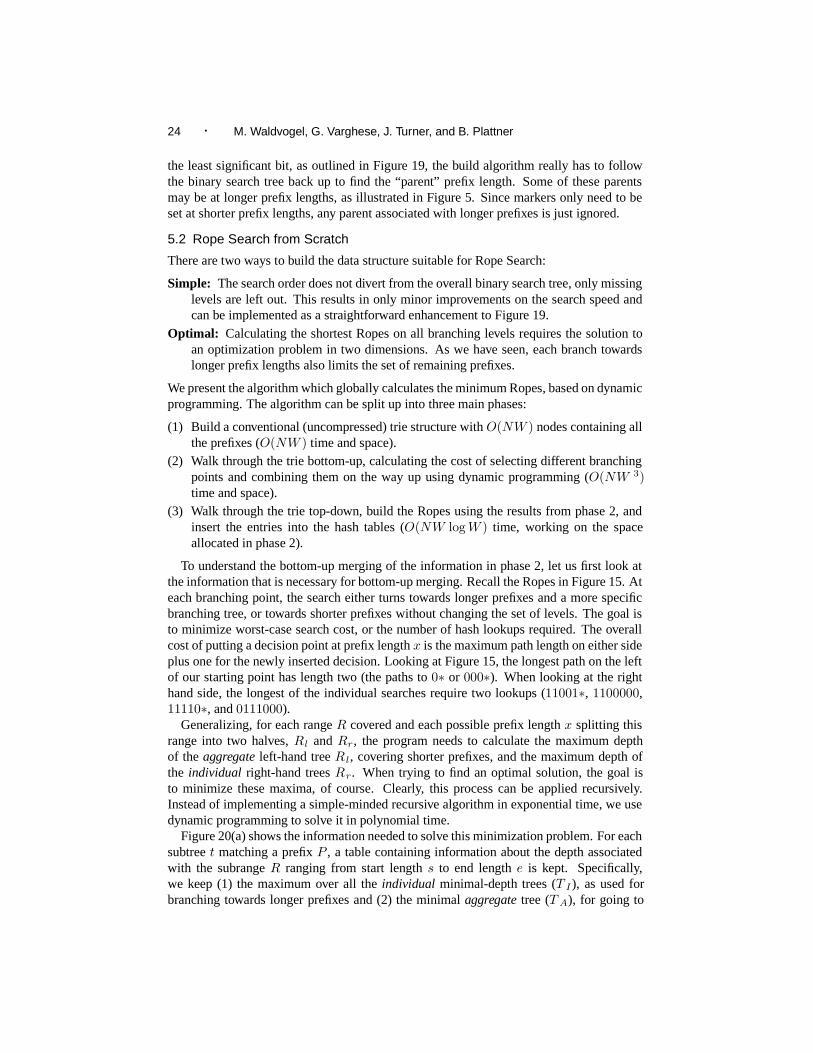
Figure 20(a) shows the information needed to solve this minimization problem. For eachsubtree t matching a prefix P , a table containing information about the depth associatedwith the subrange R ranging from start length s to end length e is kept. Specifically,we keep (1) the maximum over all the individual minimal-depth trees (T I ), as used forbranching towards longer prefixes and (2) the minimal aggregate tree (T A), for going to
Scalable High-Speed Prefix Matching · 25
Root of processed subtrie (t)
Trie's root (r)
Start(s)
End(e)
Mini- tries
Incr
easi
ng
pre
fix
len
gth
(a) Structures
Leaf set-up
Propagate
Merge
Merge+
LLL
LP+
P
M
M+
M
Incr
easi
ng
pre
fix
len
gth
Propagate+
Trie node with associated prefix
(b) Cases treated
Fig. 20. Rope Construction, Phase 2
shorter prefixes. Each of these trees in turn consists of both a left-hand aggregate tree andright-hand individual branching trees.
Using the dynamic programming paradigm, we start building a table (or in this case,a table per trie node) from the bottom of the trie towards the root. At each node, wecombine the information the children have accumulated with our local state, i.e. whetherthis node is an entry. Five cases can be identified: (L) setting up a leaf node, (P) propagatingthe aggregate/individual tables up one level, (P+) same, plus including the fact that thisnode contains a valid prefix, (M) merging the child’s aggregate/individual tables, and (M+)merging and including the current node’s prefix. As can be seen, all operations are a subsetof (M+), working on less children or not adding the current node’s prefix. Figure 21 liststhe pseudo-code for this operation.
As can be seen from Figure 21, merging the TAs takes O(W 3) time per node, with atotal of O(NW ) nodes. The full merging is only necessary at nodes with two children,shown as (M) and (M+) in Figure 20(b). In any trie, there can be only O(N) of them,resulting in an overall build time of only O(NW 3).
If the optimal next branching point is stored alongside each TA[s, e], building the ropefor any prefix in Phase 3 is a simple matter of following the chain set by these branchingpoints, by always following TA[sprev + 1, previous branching point]. A node will be usedas a marker, if the higher-level rope lists its prefix length.
5.2.1 Degrees of Freedom. The only goal of the algorithm shown in Figure 21 is tominimize the worst-case number of search steps. Most of the time multiple branchingpoints will result in the same minimal TA depth. Therefore, choosing the split point gives afurther degree of freedom to optimize other factors within the bounds set by the calculatedworst case. This freedom can be used to (1) reduce the number of entries requiring theworst case lookup time, (2) improve the average search time, (3) reduce the number ofmarkers placed, (4) reduce the number of hash collisions, or (5) improve update behavior(see below). Because of limitations in space and scope, they will not be discussed in moredepth.
26 · M. Waldvogel, G. Varghese, J. Turner, and B. Plattner
Function Phase2MergePlus;Set p to the current prefix length;
(* Merge the children’s TI below p *)Forall s, e where s ∈ [p + 1 . . . W ], e ∈ [s . . . W ];
(* Merge the TI mini-trees between Start s and End e *)If both children’s depth for TI [s, e] is 0 then
(* No prefixes in either mini-tree *)Set this node’s depth for TI [s, e] to 0;
ElseSet this node’s depth for TI [s, e] to the
the max of the children’s TI [s, e] depths;Endif
Endforall
(* “Calculate” the depth of the trees covering just this node *)If the current entry is a valid prefix then
Set TI [p, p] = TA[p, p] = 1; (* A tree with a single entry *)Else
Set TI [p, p] = TA[p, p] = 0; (* An empty tree *)Endif
(* Merge the children’s TA, extend to current level *)For s ∈ [p . . . W ];
For e ∈ [s + 1 . . . W ];(* Find the best next branching length i *)Set TA[s, e]’s depth to min(TI [s + 1, e] + 1), (* split at s *)
minei=s+1(max(TA[s, i − 1] + 1, TI [i, e]))); (* split below *)
(* Since TA[s, i − 1] is only searched after missing at i, add 1 *)Endfor
Endfor
(* “Calculate” the TI at p also *)Set TI [p, ∗] to TA[p, ∗; (* Only one tree, so aggregated=individual *)
Fig. 21. Phase 2 Pseudo-code, run at each trie node
5.3 Insertions and Deletions
As shown in [Labovitz et al. 1997], some routers receive routing update messages at highfrequencies, requiring the routers to handle these messages within a few milliseconds.Luckily for the forwarding tables, most of the routing messages in these bursts are ofpathological nature and do not require any change in the routing or forwarding tables.Also, most routing updates involve only a change in the route and do not add or deleteprefixes. Additionally, many wide-area routing protocols such as BGP [Rekhter and Li1995] use timers to reduce the rate of route changes, thereby delaying and batching them.Nevertheless, algorithms in want of being ready for further Internet growth should supportsub-second updates under most circumstances.
Adding entries to the forwarding database or deleting entries may be done without re-
Scalable High-Speed Prefix Matching · 27
building the whole database. The less optimized the data structure is, the easier it is tochange it.
5.3.1 Updating Basic and Asymmetric Schemes. We therefore start with basic and asym-metric schemes, which have only eliminated prefix lengths which will never be used. Inser-tion and deletion of leaf prefixes, i.e. prefixes, that do not cover others, is trivial. Insertionis done as during initial build (Figure 19). For deletion, a simple possibility is to just re-move the entry itself and not care for the remaining markers. When unused markers shouldbe deleted immediately, it is necessary to maintain per-marker reference counters. On dele-tion, the marker placement algorithm from Figure 19 is used to determine where markerswould be set, decreasing their reference count and deleting the marker when the counterreaches zero.
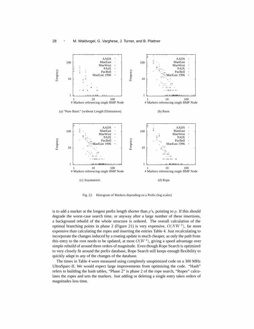
Should the prefix p being inserted or deleted cover any markers, these markers need tobe updated to point to their changed BMP. There are a number of possibilities to find allthe underlying markers. One that does not require any helper data structures, but lacksefficiency, is to either enumerate all possible longer prefixes matching our modified entry,or to walk through all hash tables associated with longer prefixes. On deletion, everymarker pointing to p will be changed to point to p’s BMP. On insertion, every markerpointing p’s current BMP and matching p will be updated to point to p. A more efficientsolution is to chain all markers pointing to a given BMP in a linked list. Still, this methodcould require O(N log W ) effort, since p can cover any amount of prefixes and markersfrom the entire forwarding database. Although the number of markers covered by anygiven prefix was small in the databases we analyzed (see Figure 22), Section 6 presents asolution to bound the update efforts, which is important for applications requiring real-timeguarantees.
During the previous explanation, we have assumed that the prefix being inserted had alength which was already used in the database. In Asymmetric Search, this may not al-ways be true. Depending on the structure of the binary search trie around the new prefixlength, adding it is trivial. The addition of length 5 in Figure 23(a) is one of these exam-ples. Adding length 6 in Figure 23(b) is not as easy. One possibility, shown in the upperexample, is to re-balance the trie structure, which unlike balancing a B-tree can result inseveral markers being inserted: One for each pre-existing prefix not covered by our newlyinserted prefix, but covered by its parent. This structural change can also adversely affectthe average case behavior. Another possibility, shown in the lower right, is to immediatelyadd the new prefix length, possibly increasing the worst case for this single prefix. Thenwe wait for a complete rebuild of the tree which takes care of the correct re-balancing.
We prefer the second solution, since it does not need more than the plain existing in-sertion procedures. It also allows for updates to take effect immediately, and only incurs anegligible performance penalty until the database has been rebuilt. To reduce the frequencyof rebuilds, the binary search tree may be constructed as to leave room for inserting themissing prefix lengths at minimal cost. A third solution would be to split a prefix into mul-tiple longer prefixes, similar to the one used by Causal Collision Resolution Section 7.1.
5.3.2 Updating Ropes. All the above insights also apply to Rope Search, and even moreso, since it uses many local asymmetric binary search trees, containing a large number ofuncovered prefix lengths. Inserting a prefix has a higher chance of adding a new prefixlength to the current search tree, but it will also confine the necessary re-balancing to asmall subset of prefixes. Therefore, we believe the simplest, yet still very efficient, strategy
28 · M. Waldvogel, G. Varghese, J. Turner, and B. Plattner
1
10
100
1 10 100
Freq
ency
# Markers referencing single BMP Node
AADSMaeEast
MaeWestPAIX
PacBellMaeEast 1996
(a) “Pure Basic” (without Length Elimination)
1
10
100
1 10 100
Freq
ency
# Markers referencing single BMP Node
AADSMaeEast
MaeWestPAIX
PacBellMaeEast 1996
(b) Basic
1
10
100
1 10 100
Freq
ency
# Markers referencing single BMP Node
AADSMaeEast
MaeWestPAIX
PacBellMaeEast 1996
(c) Asymmetric
1
10
100
1 10 100
Freq
ency
# Markers referencing single BMP Node
AADSMaeEast
MaeWestPAIX
PacBellMaeEast 1996
(d) Rope
Fig. 22. Histogram of Markers depending on a Prefix (log scales)
is to add a marker at the longest prefix length shorter than p’s, pointing to p. If this shoulddegrade the worst-case search time, or anyway after a large number of these insertions,a background rebuild of the whole structure is ordered. The overall calculation of theoptimal branching points in phase 2 (Figure 21) is very expensive, O(NW 3), far moreexpensive than calculating the ropes and inserting the entries Table 4. Just recalculating toincorporate the changes induced by a routing update is much cheaper, as only the path fromthis entry to the root needs to be updated, at most O(W 4), giving a speed advantage oversimple rebuild of around three orders of magnitude. Even though Rope Search is optimizedto very closely fit around the prefix database, Rope Search still keeps enough flexibility toquickly adapt to any of the changes of the database.
The times in Table 4 were measured using completely unoptimized code on a 300 MHzUltraSparc-II. We would expect large improvements from optimizing the code. “Hash”refers to building the hash tables, “Phase 2” is phase 2 of the rope search, “Ropes” calcu-lates the ropes and sets the markers. Just adding or deleting a single entry takes orders ofmagnitudes less time.
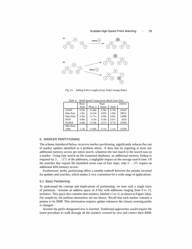
Scalable High-Speed Prefix Matching · 29
1
2
3
4
6
7
1
2
3
4
7
5
1
2
3
4
6
75
5Adding
6Adding
1
2
3
4
6
75
1
2
3
4
5
7
6
(a)
(b)
Fig. 23. Adding Prefix Lengths (Gray Nodes change Rope)
Table 4. Build Speed Comparisons (Built from Trie)Basic Rope EntriesHash Phase 2 Ropes Hash
AADS 0.56s 11.84s 0.59s 0.79s 24218Mae-East 1.82s 14.10s 0.85s 1.69s 38031Mae-West 0.58s 11.71s 0.60s 0.85s 23898PAIX 0.09s 4.16s 0.18s 0.07s 5924PacBell 0.48s 11.04s 0.57s 0.73s 22850Mae-East1996 1.14s 13.08s 0.75s 1.12s 33199
6. MARKER PARTITIONING
The scheme introduced below, recursive marker partitioning, significantly reduces the costof marker updates identified as a problem above. It does this by requiring at most oneadditional memory access per entire search, whenever the last match in the search was ona marker. Using rope search on the examined databases, an additional memory lookup isrequired for 2 . . . 11% of the addresses, a negligible impact on the average search time. Ofthe searches that require the identified worst case of four steps, only 0 . . . 2% require anadditional fifth memory access.
Furthermore, prefix partitioning offers a tunable tradeoff between the penalty incurredfor updates and searches, which makes it very convenient for a wide range of applications.
6.1 Basic Partitioning
To understand the concept and implications of partitioning, we start with a single layerof partitions. Assume an address space of 4 bits with addresses ranging from 0 to 15,inclusive. This space also contains nine markers, labeled a1 to c3, as shown in Figure 24(a).For simplicity, the prefixes themselves are not shown. Recall that each marker contains apointer to its BMP. This information requires update whenever the closest covering prefixis changed.
Assume the prefix designated new is inserted. Traditional approaches would require theinsert procedure to walk through all the markers covered by new and correct their BMP,
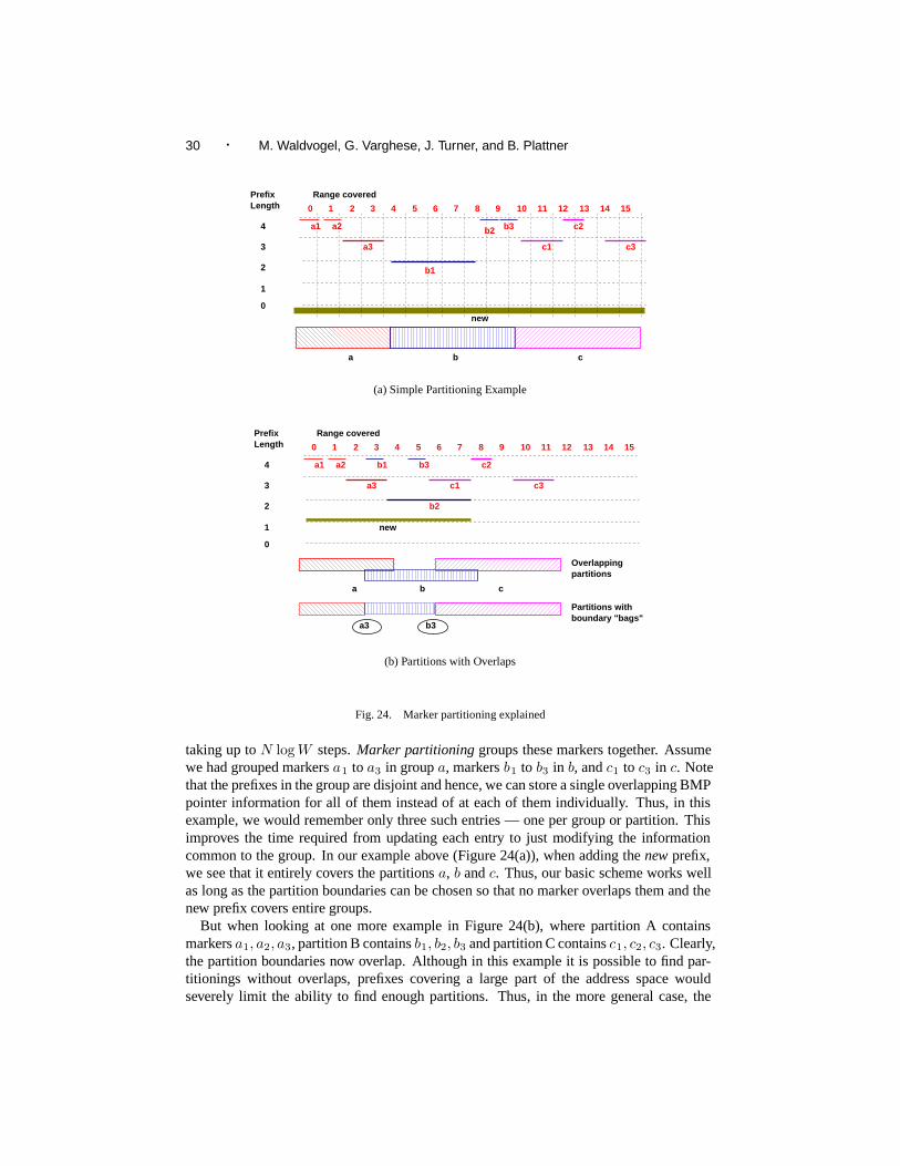
30 · M. Waldvogel, G. Varghese, J. Turner, and B. Plattner
0 1 2 3 4 5 6 7 8 9 10 11 12 13 14 15
a1 a2
a3
b1
b3b2
c1
c2
c3
PrefixLength
Range covered
4
3
2
1
0new
a b c
(a) Simple Partitioning Example
0 1 2 3 4 5 6 7 8 9 10 11 12 13 14 15
a1 a2
a3
b1 b3
b2
c1
c2
c3
PrefixLength
Range covered
4
3
2
1
0
new
a b c
Overlappingpartitions
Partitions withboundary "bags"
a3 b3
(b) Partitions with Overlaps
Fig. 24. Marker partitioning explained
taking up to N log W steps. Marker partitioning groups these markers together. Assumewe had grouped markers a1 to a3 in group a, markers b1 to b3 in b, and c1 to c3 in c. Notethat the prefixes in the group are disjoint and hence, we can store a single overlapping BMPpointer information for all of them instead of at each of them individually. Thus, in thisexample, we would remember only three such entries — one per group or partition. Thisimproves the time required from updating each entry to just modifying the informationcommon to the group. In our example above (Figure 24(a)), when adding the new prefix,we see that it entirely covers the partitions a, b and c. Thus, our basic scheme works wellas long as the partition boundaries can be chosen so that no marker overlaps them and thenew prefix covers entire groups.
But when looking at one more example in Figure 24(b), where partition A containsmarkers a1, a2, a3, partition B contains b1, b2, b3 and partition C contains c1, c2, c3. Clearly,the partition boundaries now overlap. Although in this example it is possible to find par-titionings without overlaps, prefixes covering a large part of the address space wouldseverely limit the ability to find enough partitions. Thus, in the more general case, the
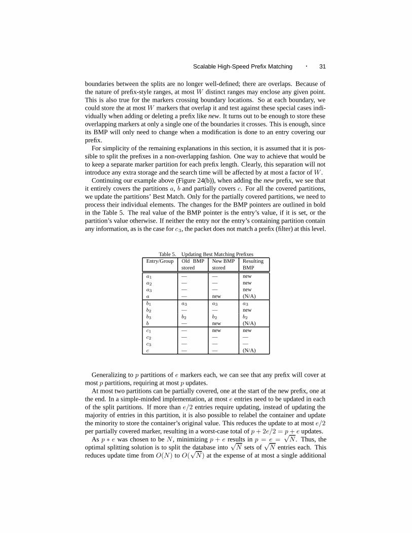
Scalable High-Speed Prefix Matching · 31
boundaries between the splits are no longer well-defined; there are overlaps. Because ofthe nature of prefix-style ranges, at most W distinct ranges may enclose any given point.This is also true for the markers crossing boundary locations. So at each boundary, wecould store the at most W markers that overlap it and test against these special cases indi-vidually when adding or deleting a prefix like new. It turns out to be enough to store theseoverlapping markers at only a single one of the boundaries it crosses. This is enough, sinceits BMP will only need to change when a modification is done to an entry covering ourprefix.
For simplicity of the remaining explanations in this section, it is assumed that it is pos-sible to split the prefixes in a non-overlapping fashion. One way to achieve that would beto keep a separate marker partition for each prefix length. Clearly, this separation will notintroduce any extra storage and the search time will be affected by at most a factor of W .
Continuing our example above (Figure 24(b)), when adding the new prefix, we see thatit entirely covers the partitions a, b and partially covers c. For all the covered partitions,we update the partitions’ Best Match. Only for the partially covered partitions, we need toprocess their individual elements. The changes for the BMP pointers are outlined in boldin the Table 5. The real value of the BMP pointer is the entry’s value, if it is set, or thepartition’s value otherwise. If neither the entry nor the entry’s containing partition containany information, as is the case for c3, the packet does not match a prefix (filter) at this level.
Table 5. Updating Best Matching PrefixesEntry/Group Old BMP
storedNew BMPstored
ResultingBMP
a1 — — newa2 — — newa3 — — newa — new (N/A)b1 a3 a3 a3
b2 — — newb3 b2 b2 b2b — new (N/A)c1 — new newc2 — — —c3 — — —c — — (N/A)
Generalizing to p partitions of e markers each, we can see that any prefix will cover atmost p partitions, requiring at most p updates.
At most two partitions can be partially covered, one at the start of the new prefix, one atthe end. In a simple-minded implementation, at most e entries need to be updated in eachof the split partitions. If more than e/2 entries require updating, instead of updating themajority of entries in this partition, it is also possible to relabel the container and updatethe minority to store the container’s original value. This reduces the update to at most e/2per partially covered marker, resulting in a worst-case total of p + 2e/2 = p + e updates.
As p ∗ e was chosen to be N , minimizing p + e results in p = e =√
N . Thus, theoptimal splitting solution is to split the database into
√N sets of
√N entries each. This
reduces update time from O(N) to O(√
N) at the expense of at most a single additional
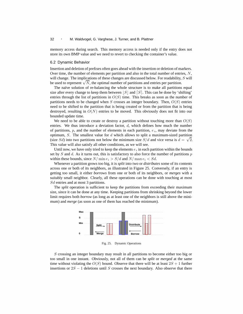
32 · M. Waldvogel, G. Varghese, J. Turner, and B. Plattner
memory access during search. This memory access is needed only if the entry does notstore its own BMP value and we need to revert to checking the container’s value.
6.2 Dynamic Behavior
Insertion and deletion of prefixes often goes ahead with the insertion or deletion of markers.Over time, the number of elements per partition and also in the total number of entries, N ,will change. The implications of these changes are discussed below. For readability, S willbe used to represent
√N , the optimal number of partitions and entries per partition.
The naıve solution of re-balancing the whole structure is to make all partitions equalsize after every change to keep them between S and �S�. This can be done by ‘shifting’entries through the list of partitions in O(S) time. This breaks as soon as the number ofpartitions needs to be changed when S crosses an integer boundary. Then, O(S) entriesneed to be shifted to the partition that is being created or from the partition that is beingdestroyed, resulting in O(N) entries to be moved. This obviously does not fit into ourbounded update time.
We need to be able to create or destroy a partition without touching more than O(S)entries. We thus introduce a deviation factor, d, which defines how much the numberof partitions, p, and the number of elements in each partition, e i, may deviate from theoptimum, S. The smallest value for d which allows to split a maximum-sized partition(size Sd) into two partitions not below the minimum size S/d and vice versa is d =
√2.
This value will also satisfy all other conditions, as we will see.Until now, we have only tried to keep the elements e i in each partition within the bounds
set by S and d. As it turns out, this is satisfactory to also force the number of partitions pwithin these bounds, since N/min ei > S/d and N/ max ei < Sd.
Whenever a partition grows too big, it is split into two or distributes some of its contentsacross one or both of its neighbors, as illustrated in Figure 25. Conversely, if an entry isgetting too small, it either borrows from one or both of its neighbors, or merges with asuitably small neighbor. Clearly, all these operations can be done with touching at mostSd entries and at most 3 partitions.
The split operation is sufficient to keep the partitions from exceeding their maximumsize, since it can be done at any time. Keeping partitions from shrinking beyond the lowerlimit requires both borrow (as long as at least one of the neighbors is still above the mini-mum) and merge (as soon as one of them has reached the minimum).
0
S
Max
MinSplit
Merge Borrow
Distribute
Fig. 25. Dynamic Operations
S crossing an integer boundary may result in all partitions to become either too big ortoo small in one instant. Obviously, not all of them can be split or merged at the sametime without violating the O(S) bound. Observe that there will be at least 2S + 1 furtherinsertions or 2S − 1 deletions until S crosses the next boundary. Also observe that there
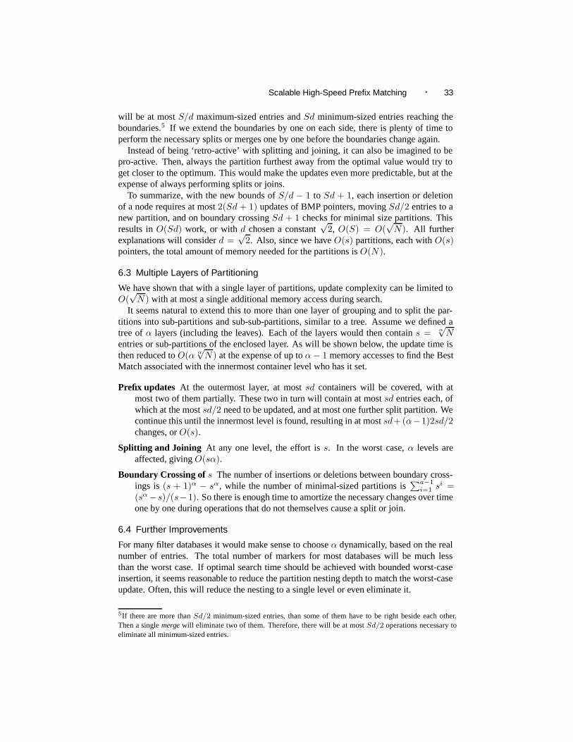
Scalable High-Speed Prefix Matching · 33
will be at most S/d maximum-sized entries and Sd minimum-sized entries reaching theboundaries.5 If we extend the boundaries by one on each side, there is plenty of time toperform the necessary splits or merges one by one before the boundaries change again.
Instead of being ‘retro-active’ with splitting and joining, it can also be imagined to bepro-active. Then, always the partition furthest away from the optimal value would try toget closer to the optimum. This would make the updates even more predictable, but at theexpense of always performing splits or joins.
To summarize, with the new bounds of S/d − 1 to Sd + 1, each insertion or deletionof a node requires at most 2(Sd + 1) updates of BMP pointers, moving Sd/2 entries to anew partition, and on boundary crossing Sd + 1 checks for minimal size partitions. Thisresults in O(Sd) work, or with d chosen a constant
√2, O(S) = O(
√N). All further
explanations will consider d =√
2. Also, since we have O(s) partitions, each with O(s)pointers, the total amount of memory needed for the partitions is O(N).
6.3 Multiple Layers of Partitioning
We have shown that with a single layer of partitions, update complexity can be limited toO(
√N) with at most a single additional memory access during search.
It seems natural to extend this to more than one layer of grouping and to split the par-titions into sub-partitions and sub-sub-partitions, similar to a tree. Assume we defined atree of α layers (including the leaves). Each of the layers would then contain s = α
√N
entries or sub-partitions of the enclosed layer. As will be shown below, the update time isthen reduced to O(α α
√N) at the expense of up to α − 1 memory accesses to find the Best
Match associated with the innermost container level who has it set.
Prefix updates At the outermost layer, at most sd containers will be covered, with atmost two of them partially. These two in turn will contain at most sd entries each, ofwhich at the most sd/2 need to be updated, and at most one further split partition. Wecontinue this until the innermost level is found, resulting in at most sd+(α−1)2sd/2changes, or O(s).
Splitting and Joining At any one level, the effort is s. In the worst case, α levels areaffected, giving O(sα).
Boundary Crossing of s The number of insertions or deletions between boundary cross-ings is (s + 1)α − sα, while the number of minimal-sized partitions is
∑a−1i=1 si =
(sα−s)/(s−1). So there is enough time to amortize the necessary changes over timeone by one during operations that do not themselves cause a split or join.
6.4 Further Improvements
For many filter databases it would make sense to choose α dynamically, based on the realnumber of entries. The total number of markers for most databases will be much lessthan the worst case. If optimal search time should be achieved with bounded worst-caseinsertion, it seems reasonable to reduce the partition nesting depth to match the worst-caseupdate. Often, this will reduce the nesting to a single level or even eliminate it.
5If there are more than Sd/2 minimum-sized entries, than some of them have to be right beside each other.Then a single merge will eliminate two of them. Therefore, there will be at most Sd/2 operations necessary toeliminate all minimum-sized entries.
34 · M. Waldvogel, G. Varghese, J. Turner, and B. Plattner
7. FAST HASHING WITH BOUNDED COLLISIONS
Many algorithms are known for hashing. Since we have mentioned a single memory accessper lookup, the number of collisions needs to be tightly bounded. One well-known solutionis perfect hashing [Fredman et al. 1984]. Unfortunately, true perfect hashing requires enor-mous amounts of time to build the hash tables and also requires complex functions to locatethe entries. While perfect hashing is a solution that satisfies the O(1) access requirement,it is often impractical. An improvement, dynamic perfect hashing [Dietzfelbinger et al.1994], also achieves O(1) lookup time at amortized cost of O(1) per insertion, by having atwo-level hierarchy of randomly chosen hashing functions. Thus, it requires two memoryaccesses per hash lookup, making it an attractive option.
With memory prices dropping, memory cost is no longer one of the main limiting factorin router design. Therefore, it is possible to relax the hashing requirements. First, we nolonger enforce optimal compaction, but allow for sparse hash tables. This already greatlyreduces the chances for collisions.
Second, we increase the hash bucket size. With current DRAM technologies, the costof a random access to a single bit is almost indistinguishable from accessing many bytessequentially. Modern CPUs take advantage of this and always read multiple consecutivewords, even if only a single byte is requested. The amount of memory fetched per access,called a cache line, ranges from 128 to 256 bits in modern CPUs. This cache line fetchingus to store a (small) number of entries in the same hash bucket, with no additional memoryaccess penalty (recall that for most current processors, access to main memory is muchslower than access to on-chip memory and caches or instruction execution.)
We have seen several key ingredients: randomized hash functions (usually only a singleparameter is variable), over-provisioning memory, and allowing a limited number of colli-sions, as bounded by the bucket size. By combining these ingredients into a hash function,we were able to achieve single memory access lookup with almost O(1) amortized inser-tion time.
In our implementations, we have been using several hash functions. One group of func-tions consists of non-parametric functions, each one utilizing several cheap processor in-structions to achieve data scrambling. Switching between these functions is achieved bychanging to a completely new search function, either by changing a function pointer or byoverwriting the existing function with the new one.
The other group consists of a single function which can be configured by a single param-eter, using f(Key∗Scramble)∗BucketCount, where f is a function returning the fractionalpart, Key is the key to be hashed, Scramble ∈ (0 . . . 1] is a configurable scrambling param-eter, and BucketCount is the number of available hash buckets. This function does notrequire floating point and can be implemented as fixed-point arithmetic using integer oper-ations. Since multiplication is generally fast on modern processors, calculation of the hashfunction can be hidden behind other operations. Knuth [Knuth 1998] recommends thescrambling factor to be close to the conjugated golden ratio ((
√5 − 1)/2). This function
itself gives a good tradeoff between the collision rate and the additional allocation spaceneeded.
It is possible to put all the hash entries of all prefix lengths into one big hash table, byusing just one more bit for the address and setting the first bit below the prefix length to1. This reduces the collision rate even further with the same total memory consumption.Since multiplication is considered costly in hardware, we also provide a comparison with
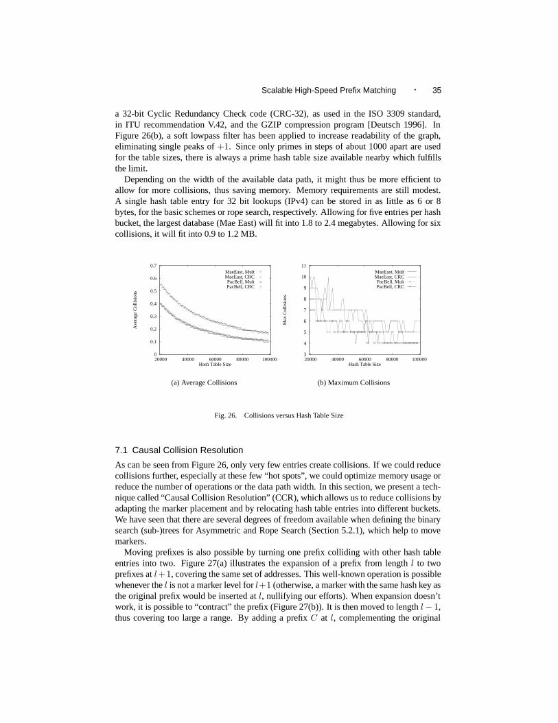
Scalable High-Speed Prefix Matching · 35
a 32-bit Cyclic Redundancy Check code (CRC-32), as used in the ISO 3309 standard,in ITU recommendation V.42, and the GZIP compression program [Deutsch 1996]. InFigure 26(b), a soft lowpass filter has been applied to increase readability of the graph,eliminating single peaks of +1. Since only primes in steps of about 1000 apart are usedfor the table sizes, there is always a prime hash table size available nearby which fulfillsthe limit.
Depending on the width of the available data path, it might thus be more efficient toallow for more collisions, thus saving memory. Memory requirements are still modest.A single hash table entry for 32 bit lookups (IPv4) can be stored in as little as 6 or 8bytes, for the basic schemes or rope search, respectively. Allowing for five entries per hashbucket, the largest database (Mae East) will fit into 1.8 to 2.4 megabytes. Allowing for sixcollisions, it will fit into 0.9 to 1.2 MB.
0
0.1
0.2
0.3
0.4
0.5
0.6
0.7
20000 40000 60000 80000 100000
Ave
rage
Col
lisio
ns
Hash Table Size
MaeEast, MultMaeEast, CRCPacBell, MultPacBell, CRC
(a) Average Collisions
3
4
5
6
7
8
9
10
11
20000 40000 60000 80000 100000
Max
Col
lisio
ns
Hash Table Size
MaeEast, MultMaeEast, CRCPacBell, MultPacBell, CRC
(b) Maximum Collisions
Fig. 26. Collisions versus Hash Table Size
7.1 Causal Collision Resolution
As can be seen from Figure 26, only very few entries create collisions. If we could reducecollisions further, especially at these few “hot spots”, we could optimize memory usage orreduce the number of operations or the data path width. In this section, we present a tech-nique called “Causal Collision Resolution” (CCR), which allows us to reduce collisions byadapting the marker placement and by relocating hash table entries into different buckets.We have seen that there are several degrees of freedom available when defining the binarysearch (sub-)trees for Asymmetric and Rope Search (Section 5.2.1), which help to movemarkers.
Moving prefixes is also possible by turning one prefix colliding with other hash tableentries into two. Figure 27(a) illustrates the expansion of a prefix from length l to twoprefixes at l+1, covering the same set of addresses. This well-known operation is possiblewhenever the l is not a marker level for l+1 (otherwise, a marker with the same hash key asthe original prefix would be inserted at l, nullifying our efforts). When expansion doesn’twork, it is possible to “contract” the prefix (Figure 27(b)). It is then moved to length l− 1,thus covering too large a range. By adding a prefix C at l, complementing the original
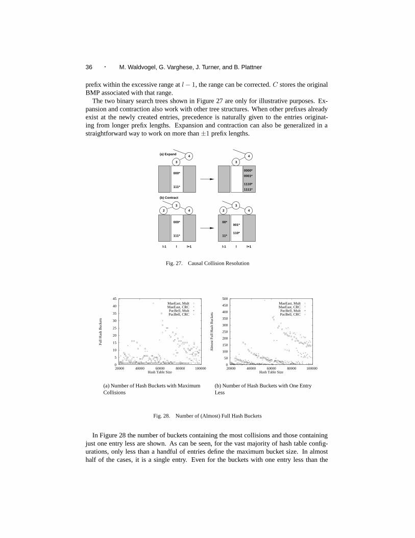
36 · M. Waldvogel, G. Varghese, J. Turner, and B. Plattner
prefix within the excessive range at l − 1, the range can be corrected. C stores the originalBMP associated with that range.
The two binary search trees shown in Figure 27 are only for illustrative purposes. Ex-pansion and contraction also work with other tree structures. When other prefixes alreadyexist at the newly created entries, precedence is naturally given to the entries originat-ing from longer prefix lengths. Expansion and contraction can also be generalized in astraightforward way to work on more than ±1 prefix lengths.
000*
111*
001*
110*
00*
11*
0000*
0001*
1110*
1111*
000*
111*
3
2 4
3
2 4
3
4
3
4(a) Expand
(b) Contract
l-1 l l+1 l-1 l l+1
Fig. 27. Causal Collision Resolution
0
5
10
15
20
25
30
35
40
45
20000 40000 60000 80000 100000
Full
Has
h B
ucke
ts
Hash Table Size
MaeEast, MultMaeEast, CRCPacBell, MultPacBell, CRC
(a) Number of Hash Buckets with MaximumCollisions
0
50
100
150
200
250
300
350
400
450
500
20000 40000 60000 80000 100000
Alm
ost F
ull H
ash
Buc
kets
Hash Table Size
MaeEast, MultMaeEast, CRCPacBell, MultPacBell, CRC
(b) Number of Hash Buckets with One EntryLess
Fig. 28. Number of (Almost) Full Hash Buckets
In Figure 28 the number of buckets containing the most collisions and those containingjust one entry less are shown. As can be seen, for the vast majority of hash table config-urations, only less than a handful of entries define the maximum bucket size. In almosthalf of the cases, it is a single entry. Even for the buckets with one entry less than the
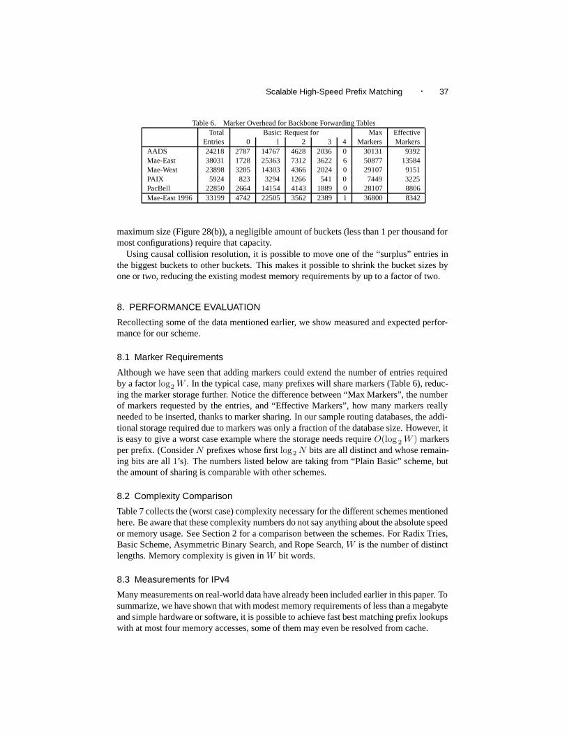
Scalable High-Speed Prefix Matching · 37
Table 6. Marker Overhead for Backbone Forwarding TablesTotal Basic: Request for Max Effective
Entries 0 1 2 3 4 Markers MarkersAADS 24218 2787 14767 4628 2036 0 30131 9392Mae-East 38031 1728 25363 7312 3622 6 50877 13584Mae-West 23898 3205 14303 4366 2024 0 29107 9151PAIX 5924 823 3294 1266 541 0 7449 3225PacBell 22850 2664 14154 4143 1889 0 28107 8806Mae-East 1996 33199 4742 22505 3562 2389 1 36800 8342
maximum size (Figure 28(b)), a negligible amount of buckets (less than 1 per thousand formost configurations) require that capacity.
Using causal collision resolution, it is possible to move one of the “surplus” entries inthe biggest buckets to other buckets. This makes it possible to shrink the bucket sizes byone or two, reducing the existing modest memory requirements by up to a factor of two.
8. PERFORMANCE EVALUATION
Recollecting some of the data mentioned earlier, we show measured and expected perfor-mance for our scheme.
8.1 Marker Requirements
Although we have seen that adding markers could extend the number of entries requiredby a factor log2 W . In the typical case, many prefixes will share markers (Table 6), reduc-ing the marker storage further. Notice the difference between “Max Markers”, the numberof markers requested by the entries, and “Effective Markers”, how many markers reallyneeded to be inserted, thanks to marker sharing. In our sample routing databases, the addi-tional storage required due to markers was only a fraction of the database size. However, itis easy to give a worst case example where the storage needs require O(log 2 W ) markersper prefix. (Consider N prefixes whose first log2 N bits are all distinct and whose remain-ing bits are all 1’s). The numbers listed below are taking from “Plain Basic” scheme, butthe amount of sharing is comparable with other schemes.
8.2 Complexity Comparison
Table 7 collects the (worst case) complexity necessary for the different schemes mentionedhere. Be aware that these complexity numbers do not say anything about the absolute speedor memory usage. See Section 2 for a comparison between the schemes. For Radix Tries,Basic Scheme, Asymmetric Binary Search, and Rope Search, W is the number of distinctlengths. Memory complexity is given in W bit words.
8.3 Measurements for IPv4
Many measurements on real-world data have already been included earlier in this paper. Tosummarize, we have shown that with modest memory requirements of less than a megabyteand simple hardware or software, it is possible to achieve fast best matching prefix lookupswith at most four memory accesses, some of them may even be resolved from cache.
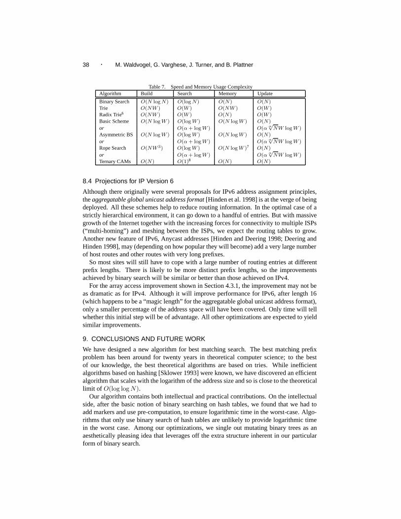
38 · M. Waldvogel, G. Varghese, J. Turner, and B. Plattner
Table 7. Speed and Memory Usage ComplexityAlgorithm Build Search Memory Update
Binary Search O(N log N) O(log N) O(N) O(N)Trie O(NW ) O(W ) O(NW ) O(W )Radix Trie6 O(NW ) O(W ) O(N) O(W )
Basic Scheme O(N log W ) O(log W ) O(N log W ) O(N)
or O(α + log W ) O(α α√
NW log W )Asymmetric BS O(N log W ) O(log W ) O(N log W ) O(N)
or O(α + log W ) O(α α√
NW log W )Rope Search O(NW3) O(log W ) O(N log W )7 O(N)
or O(α + log W ) O(αα√
NW log W )Ternary CAMs O(N) O(1)8 O(N) O(N)
8.4 Projections for IP Version 6
Although there originally were several proposals for IPv6 address assignment principles,the aggregatable global unicast address format [Hinden et al. 1998] is at the verge of beingdeployed. All these schemes help to reduce routing information. In the optimal case of astrictly hierarchical environment, it can go down to a handful of entries. But with massivegrowth of the Internet together with the increasing forces for connectivity to multiple ISPs(“multi-homing”) and meshing between the ISPs, we expect the routing tables to grow.Another new feature of IPv6, Anycast addresses [Hinden and Deering 1998; Deering andHinden 1998], may (depending on how popular they will become) add a very large numberof host routes and other routes with very long prefixes.
So most sites will still have to cope with a large number of routing entries at differentprefix lengths. There is likely to be more distinct prefix lengths, so the improvementsachieved by binary search will be similar or better than those achieved on IPv4.
For the array access improvement shown in Section 4.3.1, the improvement may not beas dramatic as for IPv4. Although it will improve performance for IPv6, after length 16(which happens to be a “magic length” for the aggregatable global unicast address format),only a smaller percentage of the address space will have been covered. Only time will tellwhether this initial step will be of advantage. All other optimizations are expected to yieldsimilar improvements.
9. CONCLUSIONS AND FUTURE WORK
We have designed a new algorithm for best matching search. The best matching prefixproblem has been around for twenty years in theoretical computer science; to the bestof our knowledge, the best theoretical algorithms are based on tries. While inefficientalgorithms based on hashing [Sklower 1993] were known, we have discovered an efficientalgorithm that scales with the logarithm of the address size and so is close to the theoreticallimit of O(log log N).
Our algorithm contains both intellectual and practical contributions. On the intellectualside, after the basic notion of binary searching on hash tables, we found that we had toadd markers and use pre-computation, to ensure logarithmic time in the worst-case. Algo-rithms that only use binary search of hash tables are unlikely to provide logarithmic timein the worst case. Among our optimizations, we single out mutating binary trees as anaesthetically pleasing idea that leverages off the extra structure inherent in our particularform of binary search.
Scalable High-Speed Prefix Matching · 39
On the practical side, we have a fast, scalable solution for IP lookups that can be imple-mented in either software or hardware, reducing the number of expensive memory accessesrequired considerably. We expect most of the characteristics of this address structure tostrengthen in the future, especially with the transition to IPv6. Even if our predictions,based on the little evidence available today, should prove to be wrong, the overall per-formance can easily be restricted to that of the basic algorithm which already performswell.
We have also shown that updates to our data structure can be very simple, with a tightbound around the expected update efforts. Furthermore, we have introduced causal colli-sion resolution which exploits domain knowledge to simplify collision resolution.
With algorithms such as ours and that of others, we believe that there is no more reasonfor router throughputs to be limited by the speed of their lookup engine. We also do notbelieve that hardware lookup engines are required because our algorithm can be imple-mented in software and still perform well. If processor speeds do not keep up with theseexpectations, extremely affordable hardware (around US$ 100) enables forwarding speedsof around 250 Gbit/s, much faster than any single transmitter can currently achieve even inthe research laboratories. Therefore, we do not believe that there is a compelling need forprotocol changes to avoid lookups as proposed in Tag and IP Switching. Even if these pro-tocol changes were accepted, fast lookup algorithms such as ours are likely to be neededat several places throughout the network.
Our algorithm has already been successfully included into the BBN multi-gigabit persecond router [Partridge et al. 1998], which can do the required Internet packet processingand forwarding decisions for 10 . . . 13 million packets per second using a single off-the-shelf microprocessor. Besides performance for IPv6, our algorithm was also chosen as itcould naturally and efficiently handle 64 bit wide prefixes (which occur while concatenat-ing destination and source addresses when forwarding IP multicast packets).
A more challenging topic beyond prefix lookups is packet classification, where multi-dimension prefix matches have to be performed, often combined with exact and rangematches. Many of the one-dimensional lookup techniques (including the one described inthis paper) have been used as lookups on individual fields, whose results are then combinedlater [Gupta and McKeown 1999; Srinivasan et al. 1998]. The main idea of this paper,namely working non-linearly in the prefix length space, has been directly generalized tomulti-dimensional packet classification schemes such as tuple space search [Srinivasanet al. 1999] and line search [Waldvogel 2000].
We believe that trie-based and CAM-based schemes will continue to dominate in IPv4-based products. However, the slow, but ongoing, trend towards IPv6 will give a strong edgeto schemes scalable in terms of prefix lengths. Except for tables where path compressionis very effective9, we believe that our algorithm will be better than trie-based algorithmsfor IPv6 routers. Perhaps our algorithm was adopted in the BBN router in anticipation ofsuch a trend.
For future work, we are attempting to fine-tune the algorithm and are looking for otherapplications. Thus we are working to improve the update behavior of the hash functionseven further, and are studying the effects of internal caching. We are also trying to optimizethe building and modification processes. Our algorithm belongs to a class of algorithms
9For instance, the initial IPv6 tables may be derived from IPv4 tables by adding a long prefix. In such cases, pathcompression will be very effective.
40 · M. Waldvogel, G. Varghese, J. Turner, and B. Plattner
that speed up search at the expense of insertion; besides packet classification, we believethat our algorithm and its improvements may be applicable in other domains besides Inter-net packet forwarding. Potential applications we are investigating include memory man-agement using variable size pages, access protection in object-oriented operating systems,and access permission management for web servers and distributed file systems.
ACKNOWLEDGMENTS
We thank V. Srinivasan, Thomas Meyer, Milind Buddhikot, Subhash Suri, and MarcelDasen for many helpful interactions, which resulted in substantial improvements of thispaper. We are also extremely grateful to have received extensive and useful comments bythe anonymous reviewers.
REFERENCES
ANDERSSON, A. AND NILSSON, S. 1994. Faster searching in tries and quadtrees – an analysis of levelcompression. In Second Annual European Symposium on Algorithms (1994), pp. 82–93.
BRAUN, F., WALDVOGEL, M., AND LOCKWOOD, J. 2001. OBIWAN – an internet protocol router inreconfigurable hardware. Technical Report WU-CS-01-xx (May), Washington University in St. Louis.
CHANDRANMENON, G. AND VARGHESE, G. 1995. Trading packet headers for packet processing. InProceedings of SIGCOMM ’95 (Boston, Aug. 1995). Also in IEEE Transactions on Networking, April1996.
CRESCENZI, P., DARDINI, L., AND GROSSI, R. 1999. IP lookups made fast and simple. In 7th AnnualEuropean Symposium on Algorithms (July 1999). Also available as technical report TR-99-01, Diparti-mento di Informatica, Universita di Pisa.
DE BERG, M., VAN KREVELD, M., AND SNOEYINK, J. 1995. Two- and three-dimensional point locationin rectangular subdivisions. Journal of Algorithms 18, 2, 256–277.
DEERING, S. AND HINDEN, R. 1998. Internet protocol, version 6 (IPv6) specification. Internet RFC2460.
DEGERMARK, M., BRODNIK, A., CARLSSON, S., AND PINK, S. 1997. Small forwarding tables for fastrouting lookups. In Proceedings of ACM SIGCOMM ’97 (Sept. 1997), pp. 3–14.
DEUTSCH, L. P. 1996. GZIP file format specification. Internet RFC 1952.
DIETZFELBINGER, M., MEHLHORN, K., ROHNERT, H., KARLIN, A., MEYER AUF DER HEIDE, F., AND
TARJAN, R. E. 1994. Dynamic perfect hashing: Upper and lower bounds. SIAM Journal of Comput-ing 23, 4, 748–761.
EATHERTON, W. N. 1999. Hardware-based Internet protocol prefix lookups. Master’s thesis, WashingtonUniversity in St. Louis, St. Louis, MO, USA.
FELDMEIER, D. C. 1988. Improving gateway performance with a routing-table cache. In Proceedings ofIEEE Infocom ’88 (New Orleans, March 1988), pp. 298–307.
FREDMAN, M. L., KOMLOS, J., AND SZEMEREDI, E. 1984. Storing a sparse table with O(1) worst caseaccess time. Journal of the ACM 31, 3, 538–544.
FULLER, V., LI, T., YU, J., AND VARADHAN, K. 1993. Classless Inter-Domain Routing (CIDR): anaddress assignment and aggregation strategy. Internet RFC 1519.
GUPTA, P., LIN, S., AND MCKEOWN, N. 1998. Routing lookups in hardware at memory access speeds.In Proceedings of IEEE Infocom (April 1998), pp. 1240–1247.
GUPTA, P. AND MCKEOWN, N. 1999. Packet classification on multiple fields. In Proceedings of ACMSIGCOMM ’99 (Cambridge, Massachusetts, USA, Sept. 1999), pp. 147–160.
GWEHENBERGER, G. 1968. Anwendung einer binaren Verweiskettenmethode beim Aufbau von Listen(Use of a binary tree structure for processing files). Elektronische Rechenanlagen 10, 223–226.
HINDEN, R. AND DEERING, S. 1998. IP version 6 addressing architecture. Internet RFC 2373.
HINDEN, R., O’DELL, M., AND DEERING, S. 1998. An IPv6 aggregatable global unicast address for-mat. Internet RFC 2374.
Scalable High-Speed Prefix Matching · 41
KNUTH, D. E. 1998. Sorting and Searching (2nd ed.), Volume 3 of The Art of Computer Programming.Addison-Wesley.
KOBAYASHI, M., MURASE, T., AND KURIYAMA, A. 2000. A longest prefix match search engine formulti-gigabit ip processing. In Proceedings of the International Conference on Communications (June2000).
LABOVITZ, C., MALAN, G. R., AND JAHANIAN, F. 1997. Internet routing instability. In Proceedings ofACM SIGCOMM ’97 (1997), pp. 115–126.
LAMPSON, B., SRINIVASAN, V., AND VARGHESE, G. 1998. IP lookups using multiway and multicol-umn search. In Proceedings of IEEE Infocom ’98 (San Francisco, 1998).
MCAULEY, A. J. AND FRANCIS, P. 1993. Fast routing table lookup using CAMs. In Proceedings ofInfocom ’93 (March–April 1993), pp. 1382–1391.
MORRISON, D. R. 1968. PATRICIA—practical algorithm to retrieve information coded in alphanumeric.Journal of the ACM 15, 514–534.
NEWMAN, P., MINSHALL, G., AND HUSTON, L. 1997. IP Switching and gigabit routers. IEEE Commu-nications Magazine 35, 1 (Jan.), 64–69.
NILSSON, S. AND KARLSSON, G. 1999. Ip address lookup using LC-tries. IEEE Journal on SelectedAreas in Communications 15, 4 (June), 1083–1092.
PARTRIDGE, C. 1996. Locality and route caches. In NSF Workshop on Internet Statistics Measure-ment and Analysis (San Diego, CA, USA, Feb. 1996). Available at http://www.caida.org/outreach/9602/positions/partridge.html.
PARTRIDGE, C., CARVEY, P. P., ET AL. 1998. A 50-gb/s IP router. IEEE/ACM Transactions on Network-ing 6, 3 (June), 237–248.
PERLMAN, R. 1992. Interconnections: Bridges and Routers. Addison-Wesley.REKHTER, Y., DAVIE, B., KATZ, D., ROSEN, E., AND SWALLOW, G. 1997. Cisco systems’ tag switch-
ing architecture overview. Internet RFC 2105.REKHTER, Y. AND LI, T. 1995. A border gateway protocol 4 (BGP-4). Internet RFC 1771.ROSEN, E. C., VISWANATHAN, A., AND CALLON, R. 2001. Multiprotocol label switching architecture.
Internet RFC 3031.RUIZ-SANCHEZ, M. A., BIERSACK, E. W., AND DABBOUS, W. 2001. Survey and taxonomy of ip
address lookup algorithms. IEEE Network 15, 2 (March–April), 8–23.SHAH, D. AND GUPTA, P. 2000. Fast incremental updates on ternary-cams for routing lookups and packet
classification. In Proceedings of Hot Interconnects (2000).SKLOWER, K. 1993. A tree-based packet routing table for Berkeley Unix. Technical report, University of
California, Berkeley. Also at http://www.cs.berkeley.edu/ ˜sklower/routing.ps.SPINNEY, B. A. 1995. Address lookup in packet data communications link, using hashing and content-
addressable memory. U.S. Patent number 5,414,704. Assignee Digital Equipment Corporation, Maynard,MA.
SRINIVASAN, V., SURI, S., AND VARGHESE, G. 1999. Packet classification using tuple space search. InProceedings of ACM SIGCOMM ’99 (Cambridge, Massachusetts, USA, Sept. 1999), pp. 135–146.
SRINIVASAN, V. AND VARGHESE, G. 1999. Fast address lookups using controlled prefix expansion.Transactions on Computer Systems 17, 1 (Feb.), 1–40.
SRINIVASAN, V., VARGHESE, G., SURI, S., AND WALDVOGEL, M. 1998. Fast and scalable layer fourswitching. In Proceedings of ACM SIGCOMM ’98 (Sept. 1998), pp. 191–202.
VAN EMDE BOAS, P. 1975. Preserving order in a forest in less than logarithmic time. In Proceedings ofthe 16th Annual Symposium on Foundations of Computer Science (1975), pp. 75–84.
VAN EMDE BOAS, P., KAAS, R., AND ZULSTRA, E. 1977. Design and implementation of an efficientpriority queue. Mathematical Systems Theory 10, 99–127.
WALDVOGEL, M. 2000. Multi-dimensional prefix matching using line search. In Proceedings of IEEELocal Computer Networks (Nov. 2000), pp. 200–207.
WALDVOGEL, M., VARGHESE, G., TURNER, J., AND PLATTNER, B. 1997. Scalable high speed IProuting table lookups. In Proceedings of ACM SIGCOMM ’97 (Sept. 1997), pp. 25–36.