schelling’s model of segregation - semantic scholar · a uniﬁed framework for schelling’s...

arX

iv:1

104.

1971

v2 [

phys

ics.

soc-

ph]

24

May

201

1 A unified framework for

Schelling’s model of segregation

Tim Rogers, Alan J. McKane

Theoretical Physics Division, School of Physics & Astronomy,

The University of Manchester, M13 9PL, UK

E-mail: [email protected], [email protected]

Abstract. Schelling’s model of segregation is one of the first and most influential

models in the field of social simulation. There are many variations of the model which

have been proposed and simulated over the last forty years, though the present state

of the literature on the subject is somewhat fragmented and lacking comprehensive

analytical treatments. In this article a unified mathematical framework for Schelling’s

model and its many variants is developed. This methodology is useful in two

regards: firstly, it provides a tool with which to understand the differences observed

between models; secondly, phenomena which appear in several model variations may

be understood in more depth through analytic studies of simpler versions.

PACS numbers: 05.40.-a, 89.75.-k, 89.65.-s

1. Introduction

The Schelling model is one of the best known mathematical models in the social sciences.

There are several reasons for this. Firstly, it is one of the oldest, having been proposed

over forty years ago [1]. Secondly, it is one of the most easily described: in the model

there are two types of individuals (agents) who tend to move if they find themselves

in regions where the other type predominates. Thirdly, it proved very successful in

illustrating a simple point, namely that only a slight homophilic bias is sufficient to

cause wholesale segregation of the two types of agents [1]. Fourthly, this finding came

http://arxiv.org/abs/1104.1971v2

A unified framework for Schelling’s model of segregation 2

at a time when the racial segregation that was occurring in US cities was at the centre

of political discussions.

While these general aspects of the Schelling model are well known, the literature

on the model since its introduction, and on its variants and generalisations, is

surprisingly disjointed and unsystematic. Part of the reason for this is that an

unusually large number of variations to the model have been proposed. Schelling

himself produced several iterations of his first model [1, 2, 3]; a consequence of

which is that there is no definitive “Schelling model”. As computing power increased

many researchers have simulated model variants related to their particular interests

[4, 5, 6, 7, 8, 9, 10, 11, 12, 13, 14, 15, 16, 17, 18, 19, 20, 21], finding segregation everywhere

from the suburbs of Tel-Aviv [15] to the Sierpinski fractal [20].

A second reason for the lack of coherence of the literature has been that the model has

attracted attention from researchers in several disciplines, who have tended to explore

different aspects of the model, often choosing adaptations which are idiosyncratic to their

own field of research. In particular, publications in the physics literature have gone to

some considerable efforts to map the Schelling model onto systems already known to

them, including liquids [22] and spin models [6, 17, 18, 19]. Whilst such analogies are

interesting, they imply that the models ought to be studied from a within particular

physical formalism, even though the corresponding assumptions, techniques and results

may not necessarily be the most relevant to the interests of researchers in other fields.

Another striking feature of the literature on the Schelling model is the strong preference

for numerical simulations over mathematical analysis. Aside from a few mathematical

papers investigating limit states of deterministic versions of the model [23, 24], analytical

results on Schelling-like models are conspicuous in their absence. Surprisingly, this

situation persists even in the physics literature where the typical models proposed are

still too complicated to admit a successful theoretical treatment and must instead be

simulated. Two recent exceptions to this are the works of Grauwin et al. [17], which maps

a Schelling-like model onto a problem amenable to equilibrium statistical mechanics, and

Dall’Asta et al. [11], with results including scaling laws for the development of clusters

of agents.

In this paper we initiate a comprehensive analysis of the Schelling model, its predictions

and generalisations. We begin in Section 2 by constructing a unified mathematical

framework for the broadest possible class of models of the Schelling type. We do this

by using the ingredients of the models studied in the literature to date, by introducing

elements motivated by models of other phenomena in the physical and biological sciences


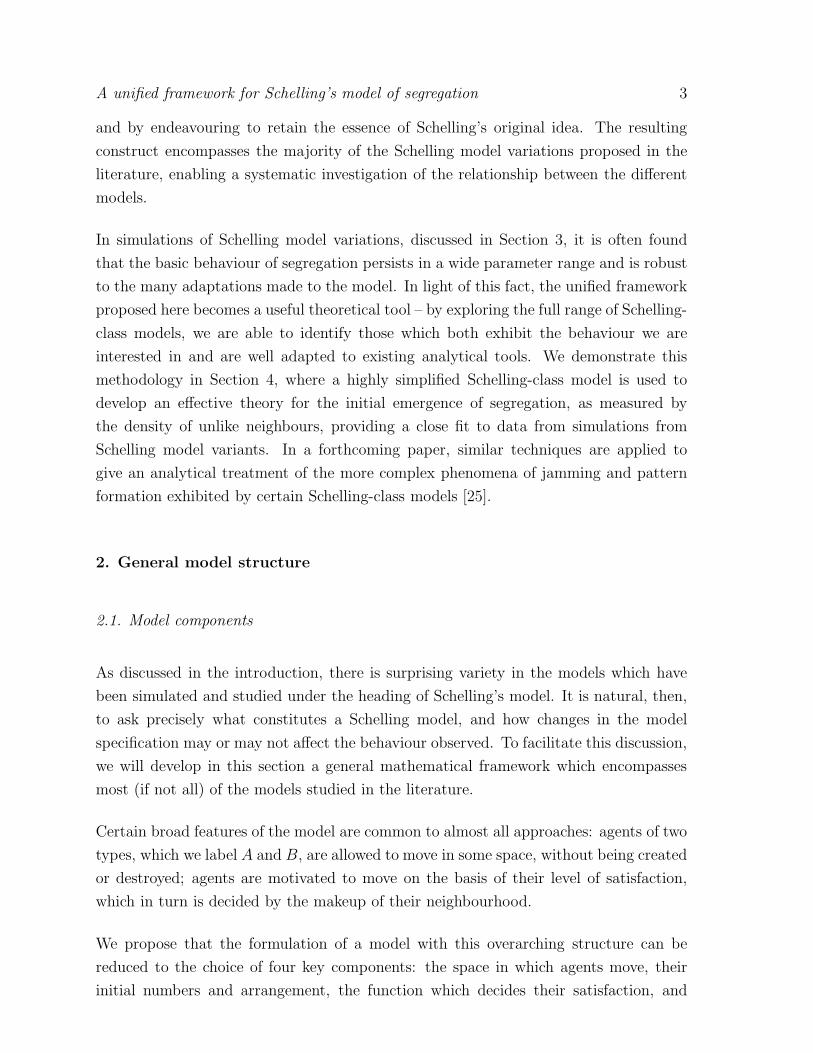
and by endeavouring to retain the essence of Schelling’s original idea. The resulting

construct encompasses the majority of the Schelling model variations proposed in the

literature, enabling a systematic investigation of the relationship between the different

models.

In simulations of Schelling model variations, discussed in Section 3, it is often found

that the basic behaviour of segregation persists in a wide parameter range and is robust

to the many adaptations made to the model. In light of this fact, the unified framework

proposed here becomes a useful theoretical tool – by exploring the full range of Schelling-

class models, we are able to identify those which both exhibit the behaviour we are

interested in and are well adapted to existing analytical tools. We demonstrate this

methodology in Section 4, where a highly simplified Schelling-class model is used to

develop an effective theory for the initial emergence of segregation, as measured by

the density of unlike neighbours, providing a close fit to data from simulations from

Schelling model variants. In a forthcoming paper, similar techniques are applied to

give an analytical treatment of the more complex phenomena of jamming and pattern

formation exhibited by certain Schelling-class models [25].

2. General model structure

2.1. Model components

As discussed in the introduction, there is surprising variety in the models which have

been simulated and studied under the heading of Schelling’s model. It is natural, then,

to ask precisely what constitutes a Schelling model, and how changes in the model

specification may or may not affect the behaviour observed. To facilitate this discussion,

we will develop in this section a general mathematical framework which encompasses

most (if not all) of the models studied in the literature.

Certain broad features of the model are common to almost all approaches: agents of two

types, which we label A and B, are allowed to move in some space, without being created

or destroyed; agents are motivated to move on the basis of their level of satisfaction,

which in turn is decided by the makeup of their neighbourhood.

We propose that the formulation of a model with this overarching structure can be

reduced to the choice of four key components: the space in which agents move, their

initial numbers and arrangement, the function which decides their satisfaction, and


lastly the mechanism for selecting if and when a particular move should take place. We

discuss these components in turn.

2.1.1. Network The concept of segregation is inherently spatial; to recognise two

groups as separate we must have some notion of when agents are close to each other

and when they are not. In Schelling’s original work this distance is geographical, with

the city divided into a grid of residences and closeness defined by one’s neighbours in

the grid [1]. One could equally well consider other ideas of distance [7, 20], for example

in terms of interpersonal relationships.

Mathematically, this situation is most easily formalised in terms of a network. We

consider a collection of N sites, joined by some number of edges. We label the sites by

the numbers 1, . . . , N . If two sites i and j are joined by an edge, we say that i and j

are neighbours in the network. The neighbourhood of i is defined to be the set of all

neighbours of i and is written ∂i. For simplicity we consider networks without multiple

edges between the same sites and without edges joining a site to itself.

At any given moment, a site may be occupied by at most one agent, or it may be vacant.

We encode the status of site i in an integer variable σi by setting

σi =

1 if site i is occupied by an agent of type A

−1 if site i is occupied by an agent of type B

0 if site i is vacant.

(1)

Using these variables, the state of the whole system at a given time (that is, the location

of each of the agents in the network) is specified by the vector σ = (σ1, . . . , σN).

The choice of encoding (1) is a common approach in the physics literature (see, for

example, [11, 18, 19]) and is useful mainly for mathematical reasons, as it provides

simple formulae for several quantities we may be interested in. For example, for any

two sites i and j,

σiσj =

1 if i and j are occupied by agents of the same type

−1 if i and j are occupied by agents of different types

0 if either site is vacant.

Note that we have made the sites, rather than the agents, into the primary objects


of interest – all agents of the same type are seen to be equivalent, and we are only

concerned with which sites they occupy.

In some of the more complicated Schelling-inspired models agents are endowed with

additional properties beyond their race, for example wealth and social status [9]. This is

also true of the residences, which may, for example, have a price [26]. These additional

factors can be incorporated into the present framework by taking vector-valued site

status variables σi, in which case each property (either of the site or of the occupying

resident) is specified by an entry of the vector.

2.1.2. Initial condition In developing his models, Schelling was concerned with the

mechanisms driving the spontaneous segregation of an initially well-integrated society. It

follows that the initial state of the model should reflect a society which is not segregated

– Schelling himself chose to place agents at random without any bias [1].

Since agents are neither created nor destroyed during the course of the model dynamics,

the initial condition fixes permanently the number of agents of each type, which may or

may not be equal. Also specified is the number and location of the vacancies which in

most Schelling-class models facilitate the movement of the agents ‡

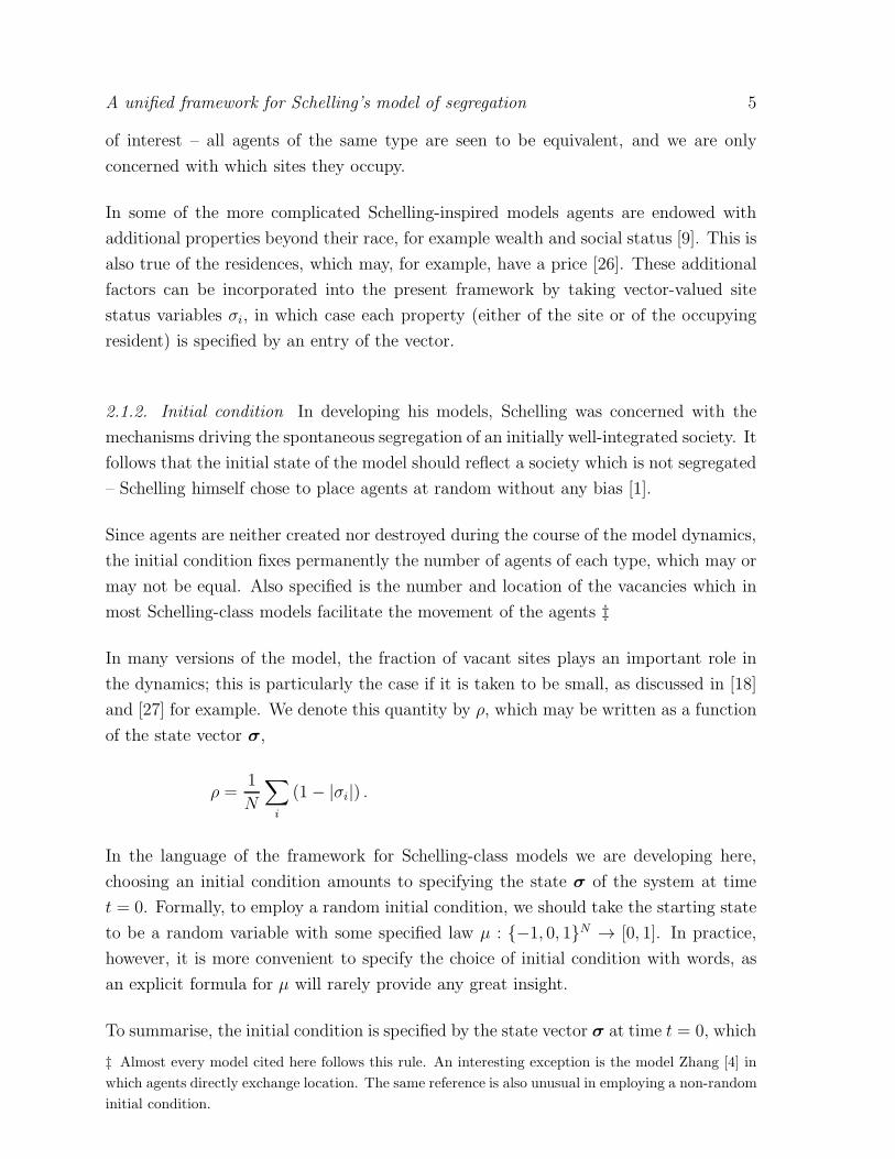
In many versions of the model, the fraction of vacant sites plays an important role in

the dynamics; this is particularly the case if it is taken to be small, as discussed in [18]

and [27] for example. We denote this quantity by ρ, which may be written as a function

of the state vector σ,

ρ =1

N

∑

i

(1− |σi|) .

In the language of the framework for Schelling-class models we are developing here,

choosing an initial condition amounts to specifying the state σ of the system at time

t = 0. Formally, to employ a random initial condition, we should take the starting state

to be a random variable with some specified law µ : {−1, 0, 1}N → [0, 1]. In practice,

however, it is more convenient to specify the choice of initial condition with words, as

an explicit formula for µ will rarely provide any great insight.

To summarise, the initial condition is specified by the state vector σ at time t = 0, which

‡ Almost every model cited here follows this rule. An interesting exception is the model Zhang [4] in

which agents directly exchange location. The same reference is also unusual in employing a non-random

initial condition.


fixes permanently the number of agents of each type, as well as the fraction of vacant

sites, denoted by ρ. In most models the initial condition will be chosen at random,

usually without any bias in the placement of agents of different types.

2.1.3. Satisfaction function In all versions of Schelling’s model, the movement of

the agents is motivated by a measure of how satisfied an agent is with its current

location and/or how satisfied it would be with a potential future location. The spirit of

Schelling’s work is captured by the general heuristic that an agent’s satisfaction should

be low if its neighbours are predominantly of the opposite type, though many different

interpretations of this requirement have been used in the past.

Introduce the vector s = (s1, . . . , sN), where the entry si is a real number between 0 and

1, encoding the satisfaction of the agent occupying site i (if i is vacant, we set si = 0).

Given the variety of different satisfaction functions used in the literature, our general

framework should be broad enough to include any sensible choice. We make no

restrictions other than to specify that satisfaction should depend only on the number

of like and unlike neighbours an agent has. Mathematically, this means that si is a

function of the numbers σiσj , for j ∈ ∂i.

Frequently in the literature the satisfaction si of an occupied site i is taken to depend on

the fraction of occupied neighbours of that site containing agents of the opposite type.

We denote this quantity by xi, where 0 ≤ xi ≤ 1, and we write xi = 0 if site i is either

vacant itself or surrounded by vacant sites, otherwise

xi =

∑

j∈∂i (|σiσj | − σiσj)

2∑

j∈∂i |σiσj |. (2)

2.1.4. Transfer probabilities Agents move either by finding a vacant site to relocate

to (leaving their starting site vacant), or in some models by directly swapping with

another agent. In either case, a move will result in two entries of the state vector being

exchanged. To express this mathematically, we introduce the notation σ(ij) for the state

vector which would result from σ if the contents of sites i and j were swapped. We also

write s(ij) for the satisfaction levels after the change. Note that this is not the same as

swapping the entries of s in positions i and j: in general s(ij)i 6= sj, as s

(ij)i specifies how

satisfied the agent currently in site i would be if it were to move to site j.

Although we have decided that agents are motivated to move by their level of


satisfaction, we have not established how a swaps should be selected or how likely a

certain swap is to take place. In short, we must choose the transfer probabilities Tij(σ),

giving the likelihood that sites i and j will be selected (in that order) and that their

contents will be swapped.

For the model to be well defined, the transfer probabilities must all be non-negative and

together satisfy for all σ,

∑

i,j

Tij(σ) = 1 ,

Write P (σ, t) for the probability that the system is in state σ at time t. The initial

condition specifies P (σ, 0), and for t > 0, the evolution of the system is determined by

the transfer probabilities according to

P (σ, t+ 1) =∑

i,j

Tij(σ(ij))P (σ(ij), t) .

Whilst in theory any variant of the Schelling model can be described in this way, it is

common in the literature (from [1] onwards) to define the model dynamics in terms of an

algorithm, rather than an explicit transfer probability. Unfortunately, the great number

of different algorithms suggested makes it difficult to place meaningful limitations on the

structure of T without ruling out potentially interesting models. This task is necessary,

however, as without constraints on T almost any dynamics could occur and it is not at

all clear how the nature of the satisfaction function and network structure is to influence

the behaviour of the model. This is one of the central difficulties in formulating a useful

mathematical framework for the study of the many variants of the Schelling model.

Our solution is to specify that Tij(σ) should be taken as the product of three components

(i) The probability of selecting the agent in site i to be given the opportunity to move

(zero if i is vacant, and non-increasing in si)

(ii) The probability of selecting site j as the destination of the move

(non-increasing in the distance from i to j)

(iii) A measure of how desirable site j is to the agent at i

(non-decreasing in s(ij)j )

It is hoped that this structure is simple and restrictive enough to make clear the way in

which the agents act selfishly to pursue their own satisfaction, whilst remaining broad


enough to include a great many of the different model variants.

2.2. Examples

In the previous subsection we developed a unified mathematical framework for Schelling-

class models, based on the specification of four components: a network, an initial

condition, a satisfaction function, and a formula to decide the transfer probabilities.

We now give some examples of Schelling-class models studied previously, showing how

the various model specifications fit within our framework.

2.2.1. Schelling As described in the introduction, the residences in Schelling’s original

two-dimensional model [1] of a city were arranged in a grid. In our framework this setting

corresponds to a two-dimensional lattice in which each site has eight neighbours (i.e. one

in each horizontal, vertical and diagonal direction). The initial condition specified by

Schelling has an equal number of agents of each type placed randomly on the network,

leaving a proportion ρ of the sites vacant. Schelling’s choice for the satisfaction function

for occupied sites is given simply by

si =

{

1 if at least half of the neighbours of i are of the same type,

0 otherwise.

The transfer probabilities are all zero except for single pair i, j with Tij(σ) = 1, where

i is the next unsatisfied site to be updated and j is the nearest vacant site which would

satisfy the agent in site i. Schelling was not entirely explicit about the precise definitions

of ‘next’ and ‘nearest’ to be used.

2.2.2. Pancs and Vriend In [8], Pancs and Vriend use the same network and initial

condition as Schelling, but make key changes to the satisfaction function and transfer

probabilities. The main alteration made is the assumption that agents select their

destination by assessing each vacant site to find the one which maximises a utility

function – this kind of ‘best response’ dynamics is a common modelling paradigm in the

economics literature.

In the model of Pancs and Vriend, the satisfaction of an occupied site i is determined

as a function u of the fraction of occupied neighbouring sites which contain an agent

of the opposite type (recall that we denote this quantity by xi). The number u(x(ij)j )


represents the utility of the site j to the agent currently in site i. The dynamics of the

model are described by the following rule: at each timestep an occupied site i is chosen

at random, the agent there moves to a vacant site j which is chosen at random from

those maximising u(x(ij)j ). The transfer probabilities resulting from this procedure may

be written explicitly using the slightly complicated expression

Tij(σ) =

( |σi|1− ρ

) (1− |σj|)I{

u(x(ij)j ) = max

ku(x

(ik)k )

}

∑

l

(1− |σl|)I{

u(x(il)l ) = max

ku(x

(ik)k )

} .

Here we have used the indicator function I, whose output is one if the argument is a

true statement and zero if it is false.

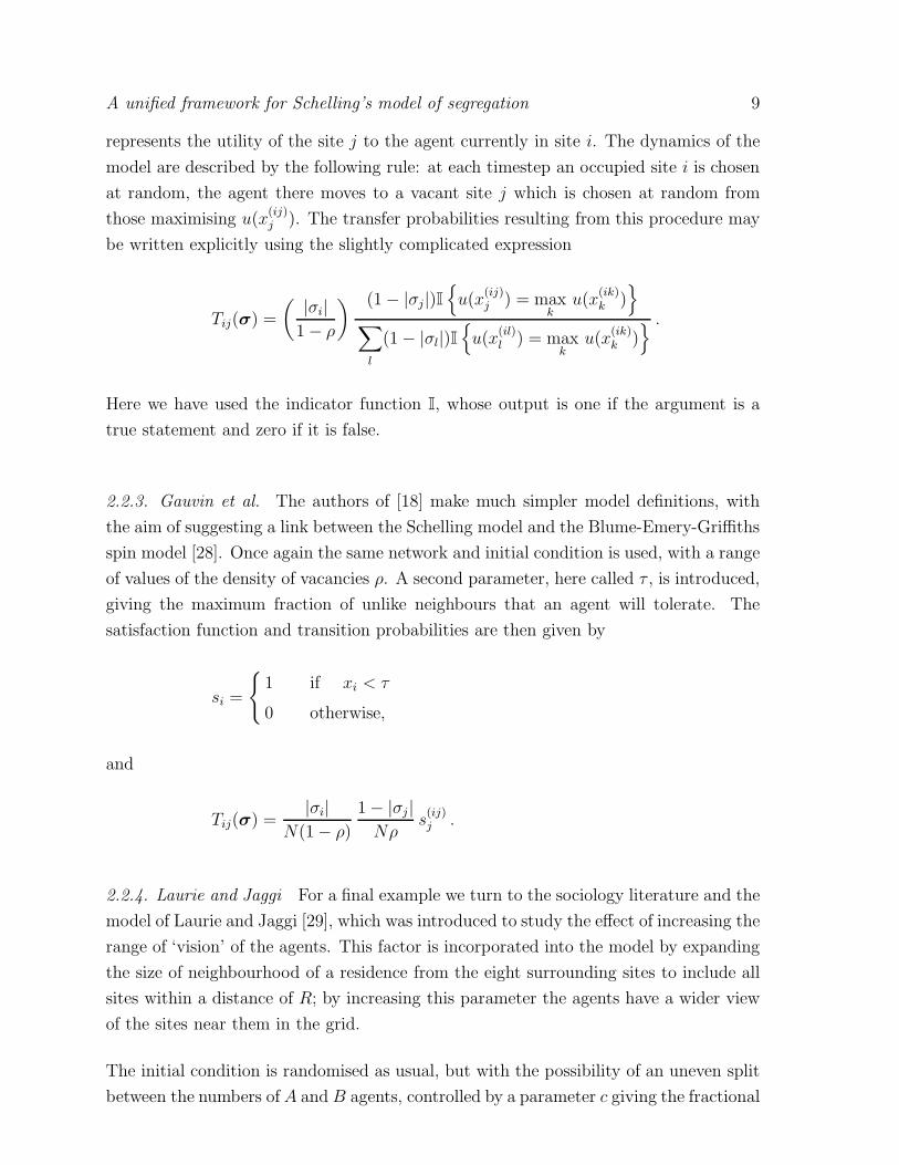
2.2.3. Gauvin et al. The authors of [18] make much simpler model definitions, with

the aim of suggesting a link between the Schelling model and the Blume-Emery-Griffiths

spin model [28]. Once again the same network and initial condition is used, with a range

of values of the density of vacancies ρ. A second parameter, here called τ , is introduced,

giving the maximum fraction of unlike neighbours that an agent will tolerate. The

satisfaction function and transition probabilities are then given by

si =

{

1 if xi < τ

0 otherwise,

and

Tij(σ) =|σi|

N(1− ρ)

1− |σj |Nρ

s(ij)j .

2.2.4. Laurie and Jaggi For a final example we turn to the sociology literature and the

model of Laurie and Jaggi [29], which was introduced to study the effect of increasing the

range of ‘vision’ of the agents. This factor is incorporated into the model by expanding

the size of neighbourhood of a residence from the eight surrounding sites to include all

sites within a distance of R; by increasing this parameter the agents have a wider view

of the sites near them in the grid.

The initial condition is randomised as usual, but with the possibility of an uneven split

between the numbers of A and B agents, controlled by a parameter c giving the fractional


size of the minority. The satisfaction function used is simply the fraction of unlike agents

in the neighbourhood. Some slight changes are also made to the dynamical rules. At

each timestep an agent is chosen; if its satisfaction is below a threshold p, it will make

up to Nρ attempts to move to a randomly selected vacancy – a given attempted move is

completed if it results in an increase to the agent’s satisfaction. The transfer probabilities

for this scheme are found by summing over number of unsuccessful attempts:

Tij(σ) =|σi|

N(1− ρ)

1− |σj |Nρ

Θ[

p− si

]

Θ[

s(ij)j − si

]

Nρ∑

n=1

(

1− 1

Nρ

∑

k

Θ[

s(ik)k − si

]

)(n−1)

,

where the Θ function gives 1 if its input is positive and 0 otherwise.

3. Simulation of existing models

3.1. Measuring segregation

Before reporting the results of simulations of whichever version of the Schelling model

one is interested in, it is first necessary to consider how the data are to be distilled into

a format which provides useful quantitative information. Schelling himself, and many

others since, have chosen to present diagrams (or latterly screenshots) showing the

arrangement of agents and vacancies at certain times. These images typically show the

emergence of patterns of agents of the same type forming domains of various shapes and

sizes. The patterns observed are striking and are no doubt responsible for generating

much interest in the model, however they are not enough on their own to provide

quantitative information about the dynamics of the system, or to compare different

parameter or model choices. In particular, this method of presenting data becomes very

much less useful if the underlying network is anything other than a square lattice, as in

[7, 20].

More sophisticated analyses of the behaviour of the system may be undertaken by

considering appropriate numerical statistics which capture some feature of the state

vector. The statistics usually considered fall broadly into two categories: those which

count the frequency of certain local configurations of agents, and those which observe

the global state of the system. We discuss the options in turn.

There are numerous ways to summarise the makeup of the neighbourhood of an

individual agent: the ratio of like to unlike, fraction of non-vacant neighbouring sites


occupied by like or unlike agents, the difference between the number of like and unlike

agents, and so on. If such a local measurement is taken at each site and the result

averaged over the whole network, one obtains an aggregate measure for the level of

segregation in the system. We choose here to focus on interface density, a frequently

studied quantity (for example in [11, 19, 20]) which is a good representative of local

statistics of this type. We define the interface density to be

x =number of edges between agents of opposite types

number of edges between agents of any type. (3)

Note that x is the average over the whole network of the local quantity xi introduced

in equation (2).

On a global scale, many Schelling-class models develop large regions filled with agents

of a single type. This behaviour is known as clustering; it might be expected that

the distribution of cluster sizes and their shape could be used to characterise model

variants. Many previous studies have numerically investigated the emergence of clusters

(examples include [8, 18, 12] and many others), however it is unfortunately very difficult

to make analytical progress in understanding cluster size distributions, even in relatively

simple spin models in statistical physics [30]. For this reason we do not focus on cluster

properties in the present study.

3.2. Simulation results

As we have seen, many different versions of the Schelling model fit within the

mathematical framework defined in the previous section, each of which can reasonably

claim to describe a simplified mechanism for the emergence of segregation. Since these

models all seek to describe the same phenomenon, one would hope that they do not

exhibit wildly different behaviour (at least away from the extremes of their parameter

space). We check this now by simulating several different Schelling-class models and

comparing the time evolution of the interface density in each model.

The models have been chosen to provide some variation in three of the four model

components: the network, the satisfaction function, and the transfer probabilities. They

are

(i) Schelling’s original 2D model [1] on a toroidal grid of N = 10, 000 sites with vacancy

density ρ = 0.1


10−1

100

101

102

103

104

105

0

0.1

0.2

0.3

0.4

0.5

Time

Inte

rfac

e D

ensi

ty

Figure 1. Time evolution of the interface density in simulations of various Schelling-

class models. Orange circles – Laurie and Jaggi [29], red diamonds – Fagiolo et al. [7],

purple stars – Schelling [1], blue triangles – Gauvin et al. [18], green squares – Pancs

and Vriend [8]. See the main text for model details and parameter values.

(ii) The best response model of Pancs and Vriend [8] on a toroidal grid of N = 10, 000

sites with vacancy density ρ = 0.1 and utility function

u(x) =

{

0.1 + 1.8 x if x ≤ 1/2

0 otherwise(4)

This choice is a particularly interesting one as it implies that agents would be most

satisfied in a mixed environment, however, in simulations segregation still emerges.

(iii) The model of Gauvin et al. [18] on a toroidal grid of N = 10, 000 sites with vacancy

density ρ = 0.1 and tolerance τ = 0.6

(iv) The model of Laurie and Jaggi [29] on a toroidal grid of N = 10, 000 sites with

neighbourhood radius R = 2, vacancy density ρ = 0.1, an equal number of each

type of agent (c = 1/2), and threshold parameter p = 0.9.

(v) A model of Fagiolo et al. [7] on a small-world network of N = 10, 000 sites and 4N

edges with rewiring probability 0.2 (see [7] for details), vacancy density ρ = 0.1,

and a Schelling-type satisfaction function.

A plot of the time evolution of the interface density for a single simulation run of each

model is shown in Figure 1. In each case time has been rescaled by a factor of N−1 to

account for system size, and again by an amount to align the curves for comparison.

There are two regimes visible in this figure. In short to medium timescales, the


simulation results show the rapid emergence of segregation in the models which, despite

significant differences in their specification, follows a single characteristic curve. This

common behaviour persists until the interface density has dropped below 0.1, by which

stage the system is already in a quite strongly segregated state. Whilst the models

considered may exhibit more unusual behaviour in certain extremes of their parameter

spaces, the results shown here are typical for a fairly broad range of ‘reasonable’

parameter choices, suggesting that the shape of curve seen above is quite robust to

changes in model specification and parameters. Consequently, it can be argued that if

one is interested in studying this behaviour then there is considerable scope to vary the

model definitions whilst keeping the analysis relevant.

After this initial segregation forming period, the different models begin to disagree

at large times as each relaxes to an equilibrium state which depends upon the model

specification, parameter choice and system size. There is variation in the nature of the

equilibrium and the mechanism of relaxation. Some models (such as that of Laurie

and Jaggi [29]) arrive at a stable configuration which does not change, either because

every agent is satisfied or because no acceptable move exists; for certain models these

limit states have been studied mathematically[23, 24]. Other models, particularly those

which allow random moves that lower the satisfaction of the agent involved (for example

Gauvin et al. [18]) reach something resembling a thermal equilibrium composed of many

similar states. Some theoretical insight may be gained into the long-time processes at

work in this case by considering the dynamics of moving groups of agents, which slowly

form larger and larger clusters [11, 18].

4. Analytical treatment

Most of the work on the Schelling model and its variants, even in the physics literature,

has been based mainly on numerical analyses of simulations. One possible reason

for the relative scarcity of analytical results is the complexity of the models usually

considered and hence the apparent difficulty of undertaking a theoretical analysis. To

make progress in a situation like this the traditional theoretical physics approach is to

choose a particular behaviour or phenomenon to investigate, and seek out new versions

of the model which capture the essential character of the problem, yet are simple enough

to study analytically.

In this section we demonstrate this principle by analysing an extremely simple Schelling-

class model, allowing us to write an effective theory for the emergence of segregation


observed in the more complex models simulated in the previous section.

4.1. Construction of a simple model

With the aim of analytically studying the emergence of segregation, we seek to construct

the simplest Schelling-class model we can. As shown in the previous section (and also in

[7]) variations in the structure of the underlying network do not appear to greatly alter

the behaviour of the model in the main parameter regime. Moreover, it is frequently

observed that network effects can greatly complicate the analysis of stochastic systems

[31]. With this in mind, we suggest to dispose of the network almost entirely, choosing

instead to group sites in pairs so that each has exactly one neighbour. This can be

thought of as an abstraction of the network in which the neighbourhood of a site is

replaced with a single representative neighbour.

With only one neighbour per site, specifying a satisfaction function amounts to picking

numbers u, v ∈ [0, 1] and setting

si =

{

u if i’s neighbour is of the same type

v otherwise.

For our model to carry the ethos of Schelling’s, we set u > v.

Continuing the pursuit of a very simple model, we take an initial condition with equal

numbers of agents of each type, placed randomly, with no vacancies. In each time step,

a randomly selected agent is allowed to move by swapping places with another (again

selected at random), according to its satisfaction before and after the swap. Specifically,

we set

Tij(σ) =1

N2(1− si)s

(ij)j . (5)

The form of this equation can be understood as follows: the N−2 factor comes from

selecting two sites (first i then j) at random from the network; the factor of (1 − si)

introduces some inertia on the part of agent i – the more satisfied they are with

their present location, the less likely they are to move; the last factor of s(ij)j is the

attractiveness of site j to the first agent selected – the move is more likely if the

destination site will provide greater satisfaction.

The combination of the network, initial condition, satisfaction function and transfer


+B

AA

B+

B

BA

A

α

β

Figure 2. A non-trivial change to the state of the simple Schelling variant discussed

in the text occurs when a pair of heterogeneous edges become homogeneous, or vice

versa. The rates α and β are determined from the parameters of the model.

probabilities given here defines almost the bare bones of a Schelling-class model. The

network has been abstracted away to a collection of disconnected pairs, the vacancies

(introduced by Schelling simply as a device to get his agents moving [1]) have been

removed, the satisfaction function is reduced to picking a pair of numbers, and the

transfer probabilities have an extremely simple form.

4.2. Deterministic limit

Write x(t) for the interface density at time t, as defined in equation (3). After analysing

the possible changes to the system in one timestep, we will take a limit of large system

size, in which a continuous time approximation is valid. As it is defined, x(t) is a

function of the state σ of the whole system, however, the relationship between the two

is sufficiently simple that it is possible to write expressions for the evolution of x(t) that

do not depend on σ.

First note that, up to a trivial renaming of the sites, one system state of this simple

model can differ from another only in regard of the number of agents which are paired

with another of a different type. By enumerating the possible choices of agents to

interact in one timestep, one finds that the only possibilities which lead to a change in

the interface density are those in which two heterogeneous pairs swap agents to become

homogeneous, or vice versa, as illustrated in Figure 2. These reactions result in a change

of ±4/N to the interface density and occur with probabilities given by (5).

The final step is to count the multiplicity of each possible arrangement. For instance,

there are Nx(t)/2 heterogeneous pairs, and hence Nx(t)(Nx(t)/2− 1) ways of choosing

two of these in order. Taking this result together with the above arguments and a similar


calculation for homogeneous pairs, we find that the interface density evolves randomly

with time according to

x(t + 1) =

x(t) +4

Nwith probability

(

1− x(t))2 (1− u)v

2

x(t)− 4

Nwith probability x(t)

(

x(t)− 2

N

)

(1− v)u

2

x(t) otherwise.

(6)

Thus, for this simple model at least, one does not require full knowledge of the system

state in order to determine the probability law governing the interface density.

If one rescales time by a factorN−1 and then takes the limitN → ∞, analysis of equation

(6) reveals that the interface density x(t) approaches a deterministic continuous time

function satisfying

dx

dt= α(1− x(t))2 − βx(t)2 , x(0) =

1

2, (7)

where α = 2(1 − u)v and β = 2(1 − v)u. The initial condition x(0) = 1/2 is simply

the average interface density in the random initial condition we specified for the simple

model. The values α and β used above are transformed parameters determining the

rate of creation and destruction of inhomogeneous edges.

The ordinary differential equation (7) is solvable, giving

x(t) =

√αβ + α tanh

(

t√αβ)

2√αβ +

(

α + β)

tanh(

t√αβ) . (8)

This result is exact for the ensemble average in the large system limit. The equilibrium

state is found by sending t → ∞, giving

x(t) −→√αβ + α

(√α +

√β)2 =

1

1 +√

β/α. (9)


10−1

100

101

102

103

0

0.1

0.2

0.3

0.4

0.5

0.6

Time

Inte

rfac

e D

ensi

ty

Figure 3. Symbols – time evolution of the interface density in a single simulation run

of each of the example models discussed in the text, see Figure 1 for details. Solid

line – analytic result for interface density of the simplified model with parameters in

equation (8) chosen to approximately fit the simulation data.

4.3. Comparison with simulations

As well as providing an exact result for the large system size limit of our highly

simplified model, the equation (7) and its solution (8) may be regarded as a simple

‘effective’ theory for the emergence of segregation in more complicated Schelling-class

models. The transformed parameters α and β can be interpreted as the average rate of

creation/destruction of inhomogeneous edges in the system. Considering the simplicity

of the theory, manipulating these parameters to fit the curve (8) to numerical data

gathered from simulations is surprisingly successful.

In Figure 3 we show the evolution of interface density in the five models considered in

the previous section over four decades in time, overlaid with the analytic result for the

simplified model, with parameters α = 0.0002 and β = 0.05 chosen to approximately

fit the simulation data. Translating these back to the model parameters u and v, we

find that the difference u − v = 0.0249 is quite a bit smaller than the typical range of

satisfaction values in the usual models. This can be understood by considering the effect

of reducing the number of neighbours per site. In a typical model with many neighbours

per site and starting from a random initial condition, most vacancies are surrounded

by a mix of different agents and hence heterogeneous edges are created and destroyed


at nearly the same rate, with only a slight imbalance due to agent preference. However

this effect is not present in the simple model with only one neighbour per site, meaning

that the timescale for segregation will be very much shorter, unless the parameters are

adjusted to compensate.

The curve (8) can in fact be made to fit several of the models rather well for very much

longer times, however, we have chosen not to show this. In the infinite network size

limit N → ∞, the long-time behaviour of the simple model is straightforward: if α > 0

the interface density approaches the non-zero equilibrium value (9), with the difference

decaying as e−2√αβ t; alternatively, if α = 0 then interface density scales as x(t) ∝ t−1.

As discussed earlier, in simulations of the more complex models it is common to observe

a scaling behaviour determined by the properties of the network and the dynamical

rules, which will eventually be limited either by the process reaching a stable state, or

by the effect of finite network size. The simplified model studied here was designed to

investigate the initial emergence of segregation rather then the long-time dynamics of

the different models, so a fit (no matter how good) to simulation data for much long

times would not be very meaningful.

It is worth reiterating that the analysis presented here is intentionally limited; we have

chosen one behavioural aspect of Schelling models and used a highly simplified model

to help us study it. Whilst the interface density is only one of several interesting

quantities which can be studied in Schelling-class models, it entirely characterises the

simple model presented here, meaning that this model can be of little interest to those

wishing to study other measures of segregation. Since there is no spatial dimension to

the model, there are no interesting screenshots to exhibit, and no discussion to be had

about pattern formation. Further, the extreme simplification made by providing each

site with only one neighbour means that this model cannot be used to study the effects of

interesting choices of satisfaction function (as in, for example [8]); the entire behaviour

is determined by two parameters describing the rate of creation and destruction of

heterogeneous edges.

We also point out that in many models one can, by exploring the extremes of the

parameter space, find radically different behaviours which do not fit the characteristic

pattern of Figure 3 and therefore cannot be reproduced by this simple model. This

should not be seen as a drawback of the present approach however; the model was

intentionally designed to investigate generic Schelling-class models in their ‘normal’

range of behaviours, and not a specific type of model in an extreme setting. In fact, the

approach advocated here, of tailoring the choice of model both to exhibit the phenomena

one wishes to study and to be accessible to the theoretical tools available, can just as


well be applied to these more unusual behaviours.

5. Conclusion

The interdisciplinary nature of research into Schelling’s model has unfortunately led to

a literature on the subject which lacks focus, with a great many different variations

of the model having been proposed and simulated. Whilst simulation is certainly a

powerful and important tool, a traditional theoretical physics approach based on the

analytic solution of a judiciously chosen simplified model can still provide a significant

contribution. In this article we have proposed a general scheme which we hope brings

some order to the catalogue of model variations and can aid with the development of

such theoretical analyses.

The principal goal of this work was to unite the many and varied generalisations to the

model in a single, simple, mathematical framework. This was achieved by identifying

four key components which together specify a Schelling-class model – the network,

the initial condition, the satisfaction function and the transfer probabilities. In each

case these components satisfy certain heuristic rules to keep them in line with spirit of

Schelling’s work, whilst being general enough to include almost all variants currently

existing in the literature.

We also discussed some of the various statistics which can be used to chart the emergence

of segregation in these models, choosing here to focus on the interface density as

a representative measure. It is worth commenting that although quantities such as

interface density can provide useful insights into the behaviour of a computation model,

a great deal of care must be taken if one hopes to infer something about segregation

in real societies. To quote Schelling, quantitative measures, of course, refer exclusively

to an artificial checkerboard and are unlikely to have any quantitative analogue in the

living world [1]. See also [27] for a related discussion on the interpretation of the model.

Moreover, the problem of quantifying segregation in real populations is itself an open

question amongst social scientists. It is beyond the scope of this article to comment on

this debate, we instead refer the interested reader to [32, 33].

One immediate benefit of approaching the plethora of variations to the model in the

systematic way developed in this article is that it allows for a structured discussion of

the changes made from one iteration to the next. For example, we see that moving from

randomly jumping agents which are popular in the physics literature [11, 18, 19] to best-


response dynamics favoured by economists [7, 8] does not result in a qualitative change

to the way in which segregation develops. Simulation results for the time evolution of

interface density in five different models taken from several disciplines were presented,

each displaying the same characteristic form in short to medium timescales.

The second useful application of the unified framework proposed here is in developing

analytically tractable models. When a particular phenomenon is observed in several

different models, careful consideration of the role of the different components used in

these models can point the way to simpler versions which will be amenable to existing

theoretical tools. To demonstrate this methodology we presented the creation and

analysis of a highly abstract form of the model, designed specifically to provide a solvable

prediction for the characteristic time dependence of interface density which was observed

in the earlier simulations. The analysis resulted in a very simple effective theory for

interface density for Schelling-class models, depending on two parameters describing

the rate of creation and destruction of homogeneous edges. These parameters can be

chosen to provide to fit simulation data from the short to medium timescales of the

more complex models.

Whilst the mathematical framework we have developed is designed to be as

comprehensive as possible, the same is not true of the analytical work presented

here, which is only a demonstration of what is possible. There are many interesting

phenomena which have manifested in simulations of Schelling-class models, and we

anticipate that most of these will be accessible to analytic treatment of carefully designed

models. Examples of future research directions include: jamming transitions when too

few vacancies are present to allow agents to move as desired; pattern formation in which

the agents spontaneously form bands of alternating types; coarsening processes and

domain growth; solid/liquid transitions depending on the likelihood of movement of

satisfied agents; the influence of stochasticity and finite size effects. In a forthcoming

paper we will show how patch-based models provide novel and analytically tractable

examples of jamming and pattern formation [25].

Acknowledgements

This work was funded by the EPSRC under grant number EP/H02171X/1.

[1] Schelling T C 1969 Am. Econ. Rev. 59 488–493

[2] Schelling T C 1971 J. Math. Sociol. 1 143–186

[3] Schelling T C 1978 Micromotives and Macrobehavior (Norton)


[4] Zhang J 2004 J. Math. Sociol. 28 147–170

[5] Fossett M 2006 J. Math. Sociol. 30 289–298

[6] Stauffer D and Solomon S 2007 Eur. Phys. J. B 57 473–479

[7] Fagiolo G, Valente M and Vriend N 2007 J. Econ. Behav. Organ. 64 316–336

[8] Pancs R and Vriend N J 2007 J. Public Econ. 91 1–24

[9] Benard S and Willer R 2007 J. Math. Sociol. 31 149–174

[10] Barr J M and Tassier T 2008 Eastern Econ. J. 34 480–503

[11] Dall’Asta L, Castellano C and Marsili M 2008 J. Stat. Mech. 2008 L07002

[12] Singh A, Vainchtein D and Weiss H 2009 Demogr. Res. 21 341–366

[13] Gracia-Lazaro C, Lafuerza L F, Florıa L M and Moreno Y 2009 Phys. Rev. E 80

[14] O’Sullivan A 2009 Reg. Sci. Urban Econ. 39 397–408

[15] Benenson I, Hatna E and Or E 2009 Sociol. Method Res. 37 463–497

[16] Fossett M and Dietrich D R 2009 Environ. Plann. B 36 149–169

[17] Grauwin S, Bertin E, Lemoy R and Jensen P 2009 P. Natl. Acad. Sci. USA 106 20622–20626

[18] Gauvin L, Vannimenus J and Nadal J P 2009 Eur. Phys. J. B 70 293–304

[19] Gauvin L, Nadal J P and Vannimenus J 2010 Phys. Rev. E 81

[20] Banos A 2010 Preprint

[21] Zhang J 2011 J. Regional Sci. 51 167–193

[22] Vinkovic D and Kirman A 2006 P. Natl. Acad. Sci. USA 103 19261–5

[23] Pollicott M 2001 Adv. Appl. Math. 27 17–40

[24] Gerhold S, Glebsky L, Schneider C, Weiss H and Zimmermann B 2008 Commun. Nonlinear Sci.

13 2236–2245

[25] Rogers T and McKane A J 2011 In Preparation

[26] Yin L 2009 Urban Stud. 46 2749–2770

[27] Edmonds B and Hales D 2005 J. Math. Sociol. 29 209–232

[28] Blume M, Emery V J and Griffiths R 1971 Phys. Rev. A 4 1071–1077

[29] Laurie A and Jaggi N 2003 Urban Stud. 40 2687–2704

[30] Bray A J 1994 Adv. Phys. 43 357–459

[31] Rogers T 2011 J Stat. Mech. 05 P05007

[32] White M J 1986 Popul. Index 52 198 – 221

[33] Simpson L 2007 J. R. Stat. Soc. A Sta. 170 405–424

schelling’s model of segregation - semantic scholar · a uniﬁed framework for schelling’s...

Documents