school of economic sciencesses.wsu.edu/wp-content/uploads/2018/02/wp2015-6-main...the usda economic...

Working Paper Series WP 2015-6

School of Economic Sciences

Measurement of U.S. Agricultural Productivity: A 2014 Review of Current

Statistics and Proposals for Change

C. Richard Shumway, Barbara M. Fraumeni, Lilyan E. Fulginiti, Jon D.

Samuels, and Spiro E. Stefanou

May 2015

Measurement of U.S. Agricultural Productivity: A 2014 Review of Current Statistics and Proposals for Change

Shumway, C. R., B. M. Fraumeni, L. E. Fulginiti, J. D. Samuels, and Spiro E Stefanou

Abstract

The USDA Economic Research Service has emerged as an acknowledged intellectual

leader in construction and integration of national and state-level productivity accounts in

agriculture. The national and state-level ERS productivity measures are widely referred to

and used, and international sectoral comparisons rely on the ERS production accounts for

foundation methodology in constructing agricultural productivity accounts in other

countries. This leadership role has endured for many decades and accelerated in response

to the AAEA-USDA Task Force review of the agricultural productivity accounts

(Gardner et al. 1980). It is with that backdrop of vigorous intellectual leadership that an

external review committee has examined the data sources, methodology, ongoing

research, documentation, and reporting of the ERS agricultural productivity accounts.

JEL Codes: O30, D24

Measurement of U.S. Agricultural Productivity: A 2014 Review of Current Statistics and

Proposals for Change

C. Richard Shumway, Barbara M. Fraumeni, Lilyan E. Fulginiti, Jon D. Samuels, and Spiro E. Stefanou

September 4, 2014

C. Richard Shumway is Regents Professor, School of Economic Sciences, Washington State University. Barbara M. Fraumeni is Special-term Professor, Central University for Finance and Economics. Lilyan E. Fulginiti is Professor, Department of Agricultural Economics, University of Nebraska. Jon D. Samuels is Research Economist, Bureau of Economic Analysis, U.S. Department of Commerce and Fellow, Institute for Quantitative Social Science, Harvard University. Spiro E. Stefanou is Professor, Department of Agricultural Economics, Sociology & Education, Pennsylvania State University and Visiting Professor of Business Economics, Wageningen University.

The authors were appointed by the U.S. Department of Agriculture (USDA), Economic Research Service (ERS), as an external committee to review the USDA Agricultural Productivity Accounts produced by the ERS. The appointment followed the Office of Management and Budget’s guidelines for the management of Federal information resources. Richard Shumway served as chair. Other authors are listed alphabetically. We wish to express appreciation for the helpful support of the ERS staff, Rachel Soloveichik, Brian Sliker, Erwin Diewert, Dale Jorgenson, Sean Cahill, Julian Alson, Philip Pardey, and to all others who responded to our invitation for stakeholder input.

The views expressed in this paper are solely those of the authors and not necessarily those of the U.S. Bureau of Economic Analysis or the U.S. Department of Commerce.

1

INDEX INTRODUCTION ............................................................................................................................................. 6

Why Undertake Another Review? ............................................................................................................ 8

Scope of This Review and Organization of the Report ............................................................................. 9

Recommendations .................................................................................................................................... 9

Overarching ........................................................................................................................................... 9

Website ................................................................................................................................................. 9

State-level ........................................................................................................................................... 10

PART 1 ......................................................................................................................................................... 11

I. Labor .................................................................................................................................................... 11

Procedure Before 1980 AAEA Task Force Recommendations ............................................................ 11

1980 AAEA Task Force Recommendations ......................................................................................... 11

ERS Implementation of 1980 AAEA Task Force Recommendations ................................................... 12

ERS Current Practice ........................................................................................................................... 12

Contract Labor (in Intermediate Inputs) ............................................................................................. 13

Recommendations .............................................................................................................................. 14

II. Non-Land Capital ................................................................................................................................. 14

Capital Measurement: General Issues ................................................................................................ 15

Equipment and Structures Capital Stock ............................................................................................ 15

Capital Input ........................................................................................................................................ 17

Inventories .......................................................................................................................................... 20

Research at BEA .................................................................................................................................. 21


III. Land .................................................................................................................................................... 21


ERS Past Implementations of 1980 AAEA Task Force Recommendations .......................................... 22



IV. Intermediate Inputs ........................................................................................................................... 24


Subsequent Guidance ......................................................................................................................... 24



V. Outputs ............................................................................................................................................... 27


2


Our Assessment .................................................................................................................................. 28


PART 2 ......................................................................................................................................................... 32

VI. Quality Adjustments .......................................................................................................................... 32

A Simple Model of Production with Quality Change .......................................................................... 32

Quality and Composition in Productivity Measurement .................................................................... 33


VII. Residual Claimants ............................................................................................................................ 36

Recommendation ................................................................................................................................ 37

VIII. Research and Development ............................................................................................................. 38

R&D in the ERS Agricultural Productivity Account .............................................................................. 38

Recommendation ................................................................................................................................ 40

IX. Alternative Assumptions .................................................................................................................... 40

Recommendation ................................................................................................................................ 41

X. Website ............................................................................................................................................... 41

Accessibility and Findability ................................................................................................................ 43

Accuracy .............................................................................................................................................. 43

Completeness ...................................................................................................................................... 43

Searchability ........................................................................................................................................ 44

Legibility .............................................................................................................................................. 44

Website and Productivity Program in Context ................................................................................... 44


PART 3 ......................................................................................................................................................... 46

XI. State-level productivity ...................................................................................................................... 46


ERS Response ...................................................................................................................................... 46

Our Assessment .................................................................................................................................. 48


XII. Cross-country comparisons............................................................................................................... 50


XIII. ERS Measures of Productivity Compared to Alternative Sources .................................................... 52

Comparison with Jorgenson, Ho, and Samuels ................................................................................... 52

Comparison with InSTePP ................................................................................................................... 53

Recommendation ................................................................................................................................ 63

3

XIV. Stakeholder Assessment .................................................................................................................. 63

CONCLUSIONS ............................................................................................................................................. 65

Recommendations .................................................................................................................................. 65

Priority A ............................................................................................................................................. 65

Priority B.............................................................................................................................................. 66

Priority C.............................................................................................................................................. 68

ACRONYMS USED IN REPORT ..................................................................................................................... 69

BIBLIOGRAPHY ............................................................................................................................................ 70

APPENDICES .…………………………………………………………………………………………………………………………………………78

Appendix 1. Personal Communication Documents to Review Committee .……………….……………...........78

Appendix 1.1. Note on user cost of capital by Brian Sliker, BEA ……………………………………….…………...78

Appendix 1.2. Document “Review Panel_Capital.docx” from V. Eldon Ball ……………………………………85

Appendix 1.3. Email exchange between Brian Sliker and Eldon Ball on capital input …………………….89

Appendix 1.4. Note on residual claimant in productivity accounts by Erwin Diewert ……………….……98

Appendix 1.5. Note on residual claimant inputs by Sean Cahill ……………………………………………………100

Appendix 2. Verbatim Stakeholder Input ……………………………………………………….………………………………110

Carlos Arnade …………………………………………………………………………………………….……………………..………..110

J. Christophe Bureau ……………………………………………………………………………………..…….……………………..112

Sean B. Cash ………………………………………………………………………………………….………..………………………….114

Jean Paul Chavas ……………………………………………………………………………………….……….……………………….115

Ramiro Costa ………………………………………………………………………………………….…………..…………………..….117

Kenneth A. Foster …………………………………………………………………………………………….…………………………120

Jose Garcia Gasques …………………………………………………………………………………………….……………………..122

Nilabja Ghosh, Anita Kumari, M. Rajeshwor ………………………………………………………….…………………….123

Wallace E. Huffman ………………………………………………………………………………………….……..………………….127

Dale Jorgenson …………………………………………………………………………………………….……………………………..128

David K. Lambert …………………………………………………………………………………………….………………………….129

Will Martin ……..…………………………………………………………………………………………….…………………………….131

Carlos San Juan Mesonada …………..……………………………………………………………….…………………………….132

Catherine Moreddu ……..……………………………………………………………………………….…………………………….133

Yair Mundlak ………………………………………………………………………………………….………………..…………………134

Alejandro Nit Pratt …………………………………………………………………………………………….…….…………………137

Christopher J. O’Donnell ………………………………………………………………………………………….….………………138

Beau Olen ………………………………………………………………………………………….……………………..………………..141

4

Richard Perrin …………………………………………………………………………………………….……………………………….142

Rulon Pope …………………………………………………………………………………………….……………………………………144

John Ruser ………………………………………………………………………………………………….……………..……………….145

Randy Schnepf ………………………………………………………………………………………….………………..………..…….146

Saleem Shaik ………..…………………………………………………………………………………….………………..…………….147

Rachel Soloveichik ……………………………………………………………………………………….……………….…………….148

Greg Strain ………..………………………………………………………………………………………….…………………………….160

Sally Thompson …………………………………………………………………………………………….…………………………….166

Keith Wiebe ………….…………………………………………………………………………………….…………………..………….167

Margaret Zeigler ………………………………………………………………………………………….…………………….……….168

5

INTRODUCTION Recent research argues that the preponderance of aggregate postwar economic growth in the U.S. was driven by investments in physical and human capital and the expansion of the labor force, while productivity growth accounted for a relatively small share of GDP growth. At the industry level, two notable exceptions to this aggregate trend were the Computer and electronic products and the Farm sectors. Innovation in the Computer and electronic products sector, exemplified by Moore’s law, has led to the proliferation of Information Technology products and the so-called Information Age. Innovation within the Farm sector has increased abundance, availability, and quality of food products, and limited price increases passed on to consumers. Understanding the sources of economic growth is crucial to economic policy (Jorgenson 2011).

The purpose of this report is to review the methods and estimates of the Agricultural Productivity Accounts developed by the Economic Research Service (ERS) of the United States Department of Agriculture (USDA). These accounts generate the official estimates of productivity in the U.S. farm sector. They include estimates of industry outputs and inputs in current and constant prices, and total factor productivity (TFP), the preferred measure of innovation according to the Advisory Committee on Measuring Innovation in the 21st Century (Schramm et al. 2008). These farm-level industry production accounts are an important contribution to the U.S. statistical system, and agricultural policy is both related to and informed by them.1

Empirical economic analysis and its conclusions are grounded in issues and concerns about data collection, variable definitions and construction, and concordance between economic concepts and statistics. Economic policy makers and scholars working on the frontiers of economic research have relied heavily on the construction of these agricultural production accounts because of their close integration of statistical concepts and economic theory. These accounts are constructed with the primary purpose of measuring the productivity of the U.S. agricultural sector. ERS has emerged as an international leader in construction and integration of these accounts in agriculture, and the national (covering all 50 states) and state-level estimates for the 48 contiguous states are widely cited as the basis for both policy and research work. The task of assembling the accounts is daunting. To match statistics with theory, assembling the accounts often involves creating data series in cases where the primary statistical base is insufficient. In some series, economic theory provides the mechanism to extrapolate from the survey data to what Gardner (1992b) refers to a “representation of facts” that generates “theory-laden data”.

A principal application of these accounts involves the measurement of agricultural productivity to build a clear picture of how the agricultural economy is performing, how it contributes to the expansion of the U.S. economy, and to identify the primary drivers of the agricultural sector’s growth. In doing so, we can determine to what extent attention should be placed on the mobilization and composition of production factors versus the advances in productivity (Jorgenson 1991). From a user’s point of view, Charles Schultze notes that productivity accounts help to keep policy makers and their economic advisors informed about the current state of the economy. He also asserts that an important avenue through which economic statistics have impact is via researchers who consume the data, conduct economic

1 The Bureau of Labor Statistics (BLS) produces Private Business Sector multi-factor productivity (MFP) that includes Farms, Private Non-Farm Business MFP, and MFP for Crop and Animal production NAICS 111, and 112 covering 1987-2011 as of July 9, 2014. ERS measures differ in the treatment of intrasectoral purchases and labor composition, they include quality adjustments for tractors, and include data back to 1947. Bureau of Economic Analysis (BEA) and BLS have produced a prototype industry-level production account that covers 1998-2012 and includes a labor composition adjustment.

6

analyses, and engage with policy advisers on appropriate policy actions and design (Schultze at al., 1991, p 423).

The agricultural accounts at the national and state levels are the subject of a wide range of investigations related to a) how intermediate inputs, labor, land and capital use patterns evolve over time and serve as factor substitutes, b) how these factors are impacted by policy, c) how technical change relates to factor use, and d) how quality adjustments are undertaken to reflect input changes and the evolving productive potential of agricultural production.

The sectoral productivity accounts are often used as a benchmark across sectors within an economy and comparison of the sectors across nations to help explain observed differences in aggregate performance and competitiveness. There is considerable interest in cross-country comparisons that investigate international competitiveness and convergence in agricultural productivity across countries. TFP growth is a standard measure employed for such comparisons. When markets are perfectly competitive and operating in long-run equilibrium, price changes can proxy for cost changes. Under these assumptions and assuming that the quality of output is the same across countries, relative output prices can proxy as a competitiveness measure for purposes of international comparisons. If countries share a common stock of knowledge and access to technologies, and if they face no structural barriers to sharing, then theory suggests that prices should change at the same rate. When we do not see this equivalence in price change, economists tend to look at policy incentives and structural differences to explain why, but the appropriate data is necessary to draw such inferences.

The notion of an aggregate production technology is the starting point for studying productivity and the sources of productivity growth. Its origins date back to Tinbergen (1942) and Solow (1957). With the need for aggregate measures of production factor and outputs, the construction of indices emerges as a necessary starting point. Balk (2008, Chapters 1 and 2) presents a historical overview of the emergence of different indices and their evolution. Jorgenson (1991) presents an extensive overview of the emergence of the approaches to measuring productivity growth with an eye toward decomposing the sources of growth. Considerable efforts are required to bridge the theory with the measurement of production factors from observed data. The challenges of adjusting for quality changes and measuring capital inputs as services are particularly difficult.

There are three key manuals governing construction of internationally comparable productivity accounts. The United Nations System of National Accounts (SNA) is an internationally standard set of recommendations on how to compile measures of economic activity. Its recommendations are expressed in terms of concepts, definitions, classifications, and accounting rules (UN, 2009). The SNA is intended for economic analysis in any country. The Organisation for Co-operation and Economic Development (OECD) Productivity Manual (2001b) serves as a standard reference of the theoretical foundations to productivity measurement, its implementation, and measurement issues. It seeks to harmonize efforts for effective international comparisons at both the aggregate and sectoral levels. The European Union Statistical Office’s (Eurostat) (2000) revised manual for constructing the Economic Accounts for Agriculture and Forestry is consistent with the SNA and addresses several specific needs of the European Union member states for sectoral accounts. Its approach is to break down the agricultural economy into production units and household units whose main source of income is agricultural.

The late 1970s found the commissioning of a joint American Agricultural Economics Association (AAEA)-USDA Task force to undertake a comprehensive review of the methodologies employed in constructing the ERS productivity accounts for U.S. agriculture and the scope these accounts covered. The outcome of this task force was a report by Gardner et al. (1980). The recommendations spanned changes in the areas of conceptual and practical productivity measurement with major recommendations to a) move from partial to total factor productivity measurement, b) address hired, operator and family labor

7

separately in the labor accounts, c) use the product approach (or specify production activities) regardless of the type of establishment in the agricultural production sector, d) account for input quality changes, and use the Divisia index to aggregate inputs and outputs (Gardner 1980, p. iii). The report also included specific suggestions related to the construction of particular input and output accounts, such as a) using the direct sampling approach to construct labor inputs, b) suggesting procedures to convert the land stock to a service flow, and c) several recommendations regarding machinery and equipment to improve the statistical data, revise the depreciation procedures, and apply the Bureau of Labor Statistics (BLS) machinery price indexes to farm machinery.

The ERS addressed the Task Force’s findings and recommendations head on and made focused efforts to bring the ERS construction of productivity accounts into harmony with state-of-the-art protocols, thus becoming an international leader in the statistical community with respect to productivity measurement. The National Agricultural Statistical Service (NASS) supports the ERS product accounts through the surveys they implement as well as by implementing the Agricultural and Resource Management Survey (ARMS) which is jointly administered with ERS.

Why Undertake Another Review? With the USDA being a principal Federal Statistical Agency, the Office of Management and Budget (OMB) mandates standards for data quality and procedural and analytic guidelines for implementing policies for the management of Federal Statistical information resources (OMB Memorandum, May 31, 2011). This also entails a regular program of data quality reviews. There is a history of external review of agricultural statistics construction and the surveys that serve as a foundation for these statistical products. In addition to the Agricultural and Applied Economics Association (AAEA)-USDA Task Force report in Gardner et al. (1980), several related reviews have been undertaken in the last three decades:

a) AAEA Statistics Committee review of USDA Farm Sector Financial Indicators, 1989-1991 (Boxley 1989);

b) General Accounting Office review of Farm Costs and Returns Survey2, 1992 (USGAO 1992);

c) AAEA Task Force on Commodity Costs and Returns, 1998-2000 (Eidman et al. 2000);

d) National Academy of Sciences Panel to review USDA's Agricultural Resource Management Survey, National Research Council, 2006-2007 (National Research Council 2007); and

e) ERS independent panel review of financial accounting methods used to summarize the Agricultural Resource Management Survey (Moss 2012).

In 2013, ERS charged our committee to address issues of methodology in the development of estimates, provide feedback on ongoing research programs to improve methodology and operations, review documentation and reporting of methods and uses of the data, and consider the frequency, timeliness, and extent of reporting. The overarching goals of the current USDA ERS Productivity Accounts review are to assess current practices used in assembling the agricultural productivity account and review how the USDA: a) documents its efforts and facilitates the ability to replicate and ensure comparability, b) describes how the community of analysts and scholars use the accounts, c) cooperates with other agencies to reduce duplication, achieve consistency across statistical series, get information at lowest cost, and capitalize on research and expertise, and d) establishes priorities subject to resource constraints.

2 The Farm Costs and Returns Survey is the predecessor to the Agricultural Resource Management Survey.

8

Scope of This Review and Organization of the Report We undertook a focused review of the ERS agricultural productivity accounts and the data products used in their construction. With the full cooperation of the USDA ERS staff that construct, maintain, and communicate analysis of these productivity accounts and related data products, this report organizes the commentary and review of the production accounts into four main parts. Each part, except for the last, includes a number of subsections.

The first part addresses the core parts of the production accounts, specifically labor, non-land capital, land, intermediate inputs, and outputs. The second addresses issues related to the construction and interpretation of the accounts. These include quality adjustments made for production factors and outputs, how residual claimants are addressed, how R&D is reflected and incorporated, the sensitivity of productivity trends to alternative assumptions, and accessibility of these data products on the website. The third addresses the state-level production accounts, cross-country comparisons, ERS measures of productivity compared to other sources, and stakeholder assessment. The final part concludes and categorizes the recommendations by priority level.

A summary of acronyms used in the report, bibliography cited, and appendices follow these four sections. This review engaged stakeholders on issues of methodology in the development of estimates, ongoing research programs to improve methodology and operations, documentation and reporting of methods and uses of the data, and the frequency and timeliness of reporting. In addition, reputed experts from academia and U.S. government and international statistical agencies external to USDA were engaged on several issues related to the ERS agricultural production accounts.3 Verbatim input from stakeholders and cited personal communications from experts in the field are included in the appendices.

Recommendations We include 21 recommendations in the top priority category. Of these, eight are designated by the committee as most important. They include two overarching recommendations, two addressing the website, and three focusing on the state-level production accounts:

Overarching

1. Fully document and keep current all procedures followed, from data sources through measurement of productivity change, to enable a non-expert to reproduce the accounts.

2. Cooperate with other agencies to reduce duplication, achieve consistency across statistical series, get information at lowest cost, and capitalize on research and expertise.

Website

1. Provide detailed documentation online and note ad hoc adjustments to data or deviations from the general procedure (e.g., if fixes were required due to negative implied capital rental rates).

2. Expand the website to provide timely access to more detailed data and procedural detail underlying the quantity and price aggregate and sub-aggregate national and state-level statistics.

3 Because the U.S. statistical system is decentralized, the ERS relies on data from other statistical agencies in assembling the agricultural productivity accounts.

9

State-level

1. Continue to develop and publish the state-level total productivity measures as well as price and quantity series (strongly recommended).

2. Cooperate with other government agencies to achieve the lowest cost method of collecting data of sufficient quality to enable the state-level accounts to be extended and maintained.

3. Investigate the possibility of using information in the American Community Survey to update matrix elements in the state labor accounts.

4. Ensure consistency between the national and state accounts where possible, and explain circumstances that prevent total consistency where that is not possible.

10

PART 1 The first section of this report reviews the components of the agricultural productivity accounts. The fundamental economic entity in the account is the industry. The farm industry as a whole produces outputs by employing labor and capital services, purchasing intermediate inputs, and transforming input to output with available technology. The ratio of output to input yields a measure of productivity, and the theory of productivity measurement provides the conditions such that the growth in output per unit of input corresponds to the change in the level of technology, or innovation. Because the productivity growth measure is a residual, all measurement problems will affect estimated TFP. In economic terms, the objective is to distinguish and measure shifts in the production function from movements along the production function.

I. Labor The OECD Productivity Manual (2001b, p. 20) states that “labor is the single most important factor of production,” thus highlighting the importance of measurement issues related to the labor input in the productivity accounts. As a partial productivity measure, changes in labor productivity (output per hour worked) help to understand the development of standards of living and income per person in an economy, but these changes embed shifts in the use of capital, the quality of the workforce, and technology. According to the ERS productivity accounts, the nominal value share of hired and family labor in U.S. agriculture output has averaged about 20 percent over the last 60 years. For accurate measurement of productivity, the labor quantity index should capture not only the hours worked but also reflect the marginal product of different types of labor working in the sector. While total hours worked is the preferred measure of the service flow for a given worker, it does not capture the heterogeneity of the labor force. Differences in skills, education, health, and professional experience lead to large differences in the contribution of different types of labor. It is necessary then to distinguish the labor input by type of skill to adequately capture the effects of changing labor quality on productivity.

Procedure Before 1980 AAEA Task Force Recommendations

Labor input data was not derived from surveys of actual hours of labor or workers in agricultural production but was calculated on a "requirements" basis using estimated quantities of labor required for various production activities. The requirement coefficients were obtained on an individual commodity basis by means of consultation with state agricultural experiment station and extension service experts. Requirement coefficients were developed for 1964 and re-done in 1974 based on cost of production surveys. The published estimates of total hours used for farm work for each of 12 enterprise groups and 10 regions (Durost and Black 1978) were obtained by multiplying labor coefficients by estimates of planted acreage (for pre-harvest labor), production (for harvest labor), or animal numbers for livestock, and adding 15% for overhead labor. The national labor input index was obtained by aggregating over the regions and enterprise groups. The U.S. average hired farm wage rate per hour as estimated by USDA's Statistical Reporting Service for 1967-69 was used in the aggregation.

1980 AAEA Task Force Recommendations

The labor input index should be based on direct sampling instead of the requirements approach.

The labor input data should be handled separately for hired, operator, and family labor, each weighted to construct an aggregate by their relative wage rates.

The Divisia index should be used for aggregation with expenditure shares as weights.

11

ERS Implementation of 1980 AAEA Task Force Recommendations

ERS has implemented the recommendations of the AAEA task force and has used theoretically consistent methods to develop Tornqvist (discrete approximation to the Divisia index) and Fisher labor input indexes for use in multifactor productivity analysis. Implementation has followed closely Jorgenson, Gollop, and Fraumeni (1987) as well as the OECD Productivity Manual (2001b).

The first set of labor indexes implementing the AAEA Task Force recommendations were reported in Ball (1985). Tornqvist indexes for the period 1948-1979 were developed that included hired labor and self-employed workers (contract labor was included in intermediate inputs). Data on wage rates as well as hours worked by characteristics of individual workers were developed by Jorgenson and Gollop and provided to ERS by Jorgenson (Ball 1985, p. 476 footnote 3). Matrices of hours worked and compensation per hour cross-classified by gender (2), age (8), education (5), employment class (2), and occupational group (10) were used.

Ball et al. (1997) developed Fisher quantity and implicit price indexes for labor for the period 1948-1994. This index included hired labor, self-employed, and unpaid family workers. Revised to include unpaid family labor in addition to operator labor, data on hours worked and average compensation were from the same sources (Ball et al. 1997, p. 1048 footnote 2). Annual data on hours worked and average compensation per hour were required for 160 matrix entries based on two genders, eight age groups, five educational groups, and two employment classes. Jorgenson and Gollop (1992) used information on employment, hours worked and average compensation from the Census of Population and the Current Population Survey along with bi-proportional matrix balancing (RAS) techniques to allocate across the matrix entries for non-census years. Additional data from the Farm Labor Survey conducted by NASS were used for unpaid family workers.

ERS has undertaken a continuous process of methodological examination and improvement as documented by the use of Tornqvist indexes for 1948-1979 in Ball (1985), Fisher indexes for 1948-1980 in Ball et al. (1997), and a new series of Tornqvist indexes4 for 1948-2011 available on the ERS Agricultural Productivity website.

ERS Current Practice

The description of current practice in this section follows Wang (2013a), the methodological description section on the Productivity Accounts on the ERS website, and information provided by direct communication with ERS.

Table 1 on the ERS website presents Tornqvist price and implicit quantity indexes for labor and its sub-components, hired and self-employed (which includes unpaid operator and family labor), for the period 1948-2011. Following Jorgenson, Gollop, and Fraumeni (1987), matrices of employment, hours worked, and compensation per hour (for hired labor) cross-classified by gender (2), age (8), education (6), and employment class (2) are used as indicated in Wang (2013a). These represent 192 entries and are slightly different than the cross-classifications used in Ball (1985) and Ball et al. (1997).

The two gender categories are: male and female.

The eight age categories are: 14-15 years, 16-17 years, 18-24 years, 25-34 years, 35-44 years, 45-54 years, 55-64 years, and 65 years and over.

The six education categories are matched to information in the Current Population Survey: 1-8 years grade school (elementary and middle school), 1-3 years high school (less than high school

4 Among other changes, the new series uses new data for labor and for land.

12

diploma), 4 years high school (high school diploma), 1-3 years college (three years of college, vocational/associates), 4 years college (bachelor’s degree), and more than four years college (graduate school, master’s degree, doctorate degree).

The two employment classes are: wage/salary worker, and self-employed/unpaid family worker.

ERS uses a cross-entropy approach in the Generalized Algebraic Modeling System (GAMS), rather than the RAS procedure in Jorgenson, Gollop and Fraumeni (1987), to update matrix elements when new information is available.

Data for hired farm workers (employment, hours worked and compensation) are from the National Income and Product Accounts (NIPA), BEA. Total hours worked for self-employed and unpaid farm workers are from the Census of Population and the Current Population Survey. Wages for self-employed and unpaid family workers are imputed using the mean wage of hired workers in the same cross-classification.

Control totals for hours worked and compensation for hired workers are from NIPA and from a special tabulation by BLS for self-employed and unpaid family workers.

The ERS implementation of the labor index, while broadly consistent with previous vintages, deviates in some ways from previously published approaches. For example, the cross tabulations used by ERS no longer contain the occupation dimension. Further, to be consistent with a change in survey questions in the Current Population Survey, updates after 1992 treat degree attained as the defining characteristic of educational attainment, compared to years of schooling in the previous estimates. Jorgenson, Ho, Stiroh (2005) discuss methods for bridging the two treatments.

Jorgenson, Ho and Samuels (2014) develop U.S. industry-level production accounts for 65 industries, including agriculture, for the period 1947-2010. As shown in Table XIII.1: Agricultural Output Growth and its Sources in this report, the evolution of the agricultural sector labor index differs from that of ERS.5 Given the overlap in source data and methods between ERS and Jorgenson, Ho and Samuels (2014), it will be important to investigate reasons for the differences across these labor indexes.

Contract Labor (in Intermediate Inputs)

Many farms, especially in fruit and vegetable production, hire labor services from contract providers. The workers are not employees of the farm, and hence are not counted as hired labor. They are reported as purchased contract labor services in intermediate inputs, and farm survey respondents are able to report expenses but not employment or hours for such workers. Because there is no available data on hours worked, ERS estimates implicit quantities of purchased contract labor services by dividing expenditures by a wage index. The data consist of nominal expenditures on contract labor. Up to 2000, ERS used ‘piece rate information’ from NASS to deflate these expenditures, but this information is no longer available. ERS has replaced this information with a wage deflator based on hedonic methods. The hedonic framework is used to estimate wage as a function of characteristics, using data from the BLS National Agricultural Workers Survey. Included are gender, years of experience, education, language skills, legal status, employer type, task type, geographic and time controls. Heckman’s procedure is used to correct for sample selection bias.

5 ERS maintains that the differences in the labor series stem in part from differences in coverage of unpaid family workers and in part from differences in the imputation of wages for farm operators.

13

Recommendations

1. Investigate the reasons for differences in the labor input computed by Jorgenson, Ho, and Samuels (2014) (Priority A).

2. Investigate the American Community Survey as an alternative, possibly complementary, data source, potentially in collaboration with BEA/BLS (Priority A).

3. Use the latest revision of information on totals from NIPA and the special BLS tabulation (Priority B).

4. Consider further refinements of the cross classification of workers to improve identification of quality differences (Priority B).

5. Adjust for temporal changes in the quality of workers in each demographic group not captured in relative wages (Priority B).

6. Clarify if the imputation of wages for self-employed workers exhausts available income and report procedures used if this occurs (Priority C).

7. Clarify how sample selection estimation is executed when the Heckman procedure is used for the contract labor hedonic wage index (Priority C).

II. Non-Land Capital Within the growth accounting framework for decomposing the sources of growth, measuring the contribution of capital input requires price and quantity estimates of the capital services that flow into production. Like labor, a key feature of the capital input measure is that it must treat a shift in the composition of capital towards an asset type with a higher marginal product as an increase in capital input used in production. Ignoring this type of composition shift amounts to a systematic bias in estimated TFP. Fortunately, research on productivity measurement has established methods to adjust for composition changes in capital services, and ERS has, for the most part, adopted these procedures.

ERS has carefully incorporated the recommendations of the AAEA Task Force (Gardner et al. 1980) that relate to non-land capital inputs. They include measuring multifactor productivity, improving the quality of data on the stocks of machinery and equipment, and modifying structures and capital equipment depreciation procedures to better reflect “economic value of services at each point of an item’s lifetime” (p. 46).

Since the 1980 review of measurement of U.S. agricultural productivity, there have been substantial developments in the measurement of productivity, particularly in the measurement of capital inputs. Two developments which occurred in the early eighties are of particular note: the publication of the book on U.S. productivity and economic growth by Jorgenson, Gollop, and Fraumeni (1987) and the first release by BLS (U.S. Department of Labor (USDOL) 1983) of multifactor productivity estimates for a number of aggregate sectors.6 Both included capital inputs in the production function.7 Similar to ERS, the BLS’s Office of Productivity and Technology (OPT) developed multifactor productivity measures as recommended by a panel review (see Rees 1979).

Later, OECD issued two capital manuals on measuring capital and one on measuring productivity (OECD 2001a, 2001b, 2009). Beginning in 2003 the European Union Capital, Labor, Energy, Materials, Services (KLEMS) project (Van Ark, O'Mahony and Ypma 2007) began to develop industry-level production accounts for European countries; subsequently this effort was extended to other countries through the

6 Earlier books on productivity and economic growth included Denison (1974) and Kendrick (1961 and 1973). 7 For detailed discussions of capital stocks and capital inputs, see Fraumeni and Jorgenson (1980), Jorgenson (1980), and Kendrick (1976).

14

World KLEMS project.8 Since most of the activity related to measurement of multifactor productivity and in particular capital inputs occurred subsequent to the 1980 review of measurement of U.S. agricultural productivity, we will not refer further to the 1980 review recommendations.

ERS’s methodology is broadly consistent with the approaches used in the literature. The majority of the implementation choices made are reasonable and defensible. The review committee, supported by productivity expert feedback (Sliker, 2014b), has identified an internal inconsistency and a deviation from a typically used approach that are addressed in more detail below.

Capital Measurement: General Issues

Measurement of capital differs from measurement of hired labor in that wages paid to hired labor are recorded, whereas rent paid to capital frequently is unrecorded because capital is more often owned than leased. Furthermore, the flow of services from the productive capital stock is unobserved, and the productive capital stock is based on the accumulation of past investments. These fundamental differences give rise to a number of difficulties and assumptions in capital measurement.

The construction of capital input begins with construction of the capital stock. The perpetual inventory method is typically used to develop real capital stock estimates:

(II.1) Kt = It + (1-δt-1)Kt-1,

where Kt is real productive capital stock in period t, It is real gross investment in period t, and δt is the rate of efficiency decline in period t. The importance of implementing capital stock construction by industry and by asset type has been demonstrated in many empirical applications.

The next step is to construct the user cost of capital for each asset, which is also called the rental price of capital services. It represents the transformation of the acquisition price of capital to the per-period usage price: 9

(II.2) pK,t = pI,t (rt + pD) - (pI,t - pI,t-1)

where pK,t, the user cost of capital, is the cost of using the capital asset in period t, pI,t is the period t market price of a new asset, rt is the period t interest cost or opportunity cost of employing capital elsewhere and is often called the rate of return, pD is the period t rate of depreciation or the rate of loss in the value of the asset as it ages, and (pI,t - pI,t-1) measures capital gains, losses, or revaluation of the asset between period t and t-1. Some statistical agencies, such as the Australian Bureau of Statistics, BLS, and researchers associated with Jorgenson, include tax in the user cost formula.

User costs are then multiplied by the real productive stocks to create nominal capital inputs (or capital flows) by asset, which are used as productive capital stock weights in an index number formula to create an aggregate real capital input. The theory of production equates these weights to be consistent with the marginal product of each capital asset.

In our review of non-land capital inputs, we focus on these two themes of capital stocks and capital inputs, the latter beginning with the construction of the user cost of capital.

Equipment and Structures Capital Stock

ERS uses three major sources for the nominal investment data: BEA fixed assets data for years prior to 1975, NASS Farm Production Expenditures Survey data for 1975-1992, and ARMS data for 1993 to the

8 See http://www.worldklems.net/index.htm for information on World KLEMS. 9 This brief user cost description closely follows OECD (2009, pp. 64-65).

15

http://www.worldklems.net/index.htm

present. There are four categories of ERS farm nominal investment data: Autos from 1926, farm tractors from 1929, buildings from 1871, and other machinery (an aggregate) from 1914.

Beginning in the year for which BEA fixed asset data are available on the internet (1901 at the earliest), the committee compared the ERS data for all years forward to the BEA fixed asset data.10 This comparison is preliminary and suggestive; it should not be construed as a precise or totally accurate analysis. However it revealed substantial differences between the current BEA data through 1974 and the ERS data, and there is no perceptible pattern of differences, except that ERS data prior to 1975 tend to be lower for equipment and higher for buildings than the BEA fixed assets data.11 Beginning in 1975, the ERS data are almost always lower for both equipment and structures.

A comparison was also made between the BEA fixed assets category for all equipment except for autos and farm tractors (other equipment) and the ERS category other equipment from 1947 to the present. With one exception, the percentage that ERS other equipment is of ERS total equipment is consistently lower than the percentage that BEA other equipment is of BEA total equipment, with differences as high as 13 percentage points before 1993. After 1987 BEA farm investment categories include computers and software and after 1992 wind and solar power.

Benchmarks and lifetimes

Since the ERS investment data go far back in time relative to the asset lifetimes, it is appropriate to assume a zero benchmark as ERS has done.

The ERS average service lives are 10 for autos, 9 for farm tractors, 17 for other machinery, and 38 for buildings. The ERS average lifetimes for farm tractors and buildings match BEA average lifetimes. BEA does not use an explicit average service life for autos; rather it develops deterioration rates from information on new and used auto prices (see U.S. Department of Commerce (USDOC) 2013).12 In addition, the BEA category “autos” refers to all autos listed under private nonresidential equipment. This category excludes autos which are classified as durables owned by consumers.13 BLS average service lives are also the same as ERS except for tractors, which is 8 years (USDOL 1983).14

10 Most of the BEA fixed asset data are available at http://www.bea.gov/national/FA2004/Details/Index.html. However, some of the early BEA data are not. 11 There are several possible reasons for these differences: The BEA fixed asset data base used by ERS has not been re-collected since it was first obtained in 1985 although BEA has revised the earlier data since then. The BEA title in the farm category under “total structures” is simply “farms”, so it is not clear if this category only refers to nonresidential farm structures. There is a separate category under the farm industry labeled “lodging” with zeroes in all entries. Patterns also differ for the equipment subcategories of tractors and autos. 12 In this review, the word deterioration is consistently used to refer to the decline in efficiency of an asset as it ages and the word depreciation to the decline in the price of an asset as it ages. This distinction is discussed in a later section. 13 Service life references in addition to USDOC (2003) include USDOC (2013), Hulten and Wykoff (1981a, 1981b), Wykoff and Hulten (1979), and Fraumeni (1997). A footnote in BEA (1983) specifies that the average service life was 8 years for producer durable equipment autos and 14 years for agricultural machinery except tractors; it is possible that the latter category includes autos used in agriculture. 14 Since the BLS category tractors does not specify farm tractors, this average life may reflect average service lives for farm and construction tractors. The source for ERS average service lives of buildings and agricultural machinery except tractors has not been updated since BEA revised its service lives in the latter nineties. See USDOC (2013) for the current BEA lifetimes which are mainly taken from Fraumeni (1997) and in most cases do not depend on Bulletin F lifetimes.

16

http://www.bea.gov/national/FA2004/Details/Index.html

Investment deflators

Investment deflators for all capital assets except buildings were obtained from BLS. The investment deflator for buildings is from BEA. More information is needed about the specific sources, e.g., whether the BLS deflators are those used in the BLS multifactor productivity estimates, whether the BEA structures deflators are those for farm buildings, and whether revisions made in BLS and BEA deflators since 1985 have been incorporated.

Deterioration and retirements

ERS estimates deterioration and retirements using methodology almost identical to that used by BLS. The deterioration function is a hyperbolic function with β equal to .75 for buildings and .5 for equipment. The ERS retirement function is a truncated normal distribution with the spread equal to double the average service life, i.e., from 1 to 20 for autos, 1 to 18 for farm tractors, 1 to 34 for other machinery, and 1 to 76 for buildings. The spread adopted by BLS is only slightly different: .02 to 1.98 times the average service life (USDOL 1983, pp. 44-45). This is the only difference between ERS and BLS methodology with respect to deterioration and retirements.15

Capital stock construction

ERS uses a perpetual inventory method to construct stocks. This methodology is also widely used by others. However, Sliker (2014b), as discussed below in the depreciation section, questions whether the aggregation procedure over individual assets is internally consistent.

Capital Input

Rate of return

The real rate of return r is calculated as the nominal yield on investment grade corporate bonds less the expected (forecasted) rate of inflation as measured by the implicit deflator for gross domestic product. An ex-ante real rate of return is obtained by expressing inflation as an ARIMA process.16 In the review panel’s opinion, it is defensible to use an expected rate of return estimated with an ARIMA process instead of an actual rate of return. It is only the choice by ERS of the GDP deflator as the expected rate of inflation measure that is unusual. In widely used approaches, the rate of asset capital gain or loss is measured by an asset-specific deflator in the real rate of return. The choice of the GDP deflator may have been dictated by common problems that researchers have when asset capital gain produces an asset-specific real rate of return which varies widely or may even be negative. However, that can be resolved by following BLS in the use of a smoothing function that takes the average rate of asset inflation over several years. Incorporating asset-specific capital gains is particularly important for assets with rapidly changing prices such as computers.

The formula for r is ((1+bond)/(1+expected inflation))-1 where the bond rate is that over all maturities for AAA rated bonds.17 The choice of the AAA bond rate as the nominal opportunity cost of invested funds stems from the fact that Farm Credit bonds are almost always rated AAA. This choice is defensible as the Farm Credit system is a major player in the agricultural credit market. In the construction of user cost of capital, r is held constant for a particular vintage of capital goods. No attempt is made to separate corporate and noncorporate capital input, which have different implicit rental prices due to

15 Prior to revising its deterioration methodology sometime after 1997, but before 2003, BEA used skewed Winfrey (1967) retirement distributions for some assets. 16 Some researchers argue for ex-post rates of return; others argue for ex-ante rates of return. There is no consensus among productivity researchers. See OECD (2001b) for a discussion. 17 See Figure XIII.2 for ERS developed real rate of return.

17

differences in tax structures by legal form. As BEA provides BLS with a corporate/noncorporate split, such a split could be implemented.18 Additional discussion on the choice of interest rate is included in the section on the Residual Claimant.

Taxation

ERS does not incorporate any tax terms into its user cost formula. This differs from the BLS (Harper 1999), Australian Bureau of Statistics (2013), and Jorgenson, Gollop, and Fraumeni (1987) practice. As noted previously, the decision to exclude tax terms may have been made either because it very significantly complicates the user cost of capital equation or because of data availability issues. Whatever the reason, an explanation is warranted.

Depreciation

To construct a measure of capital input, first a measure of capital stock is constructed followed by a measure of the user cost of capital; the latter requires a measure of depreciation, i.e. equation (II.2).19 With the perpetual inventory method of constructing capital stocks, real gross investment is accumulated and reduced by deterioration of capital stock, which differs conceptually from depreciation.20

ERS has made assumptions typically employed (for example, by BLS) to measure deterioration and create measures of capital stock. However, ERS takes a different approach to implementing the measurement of user cost, with components representing the opportunity cost of invested funds and the discounted stream of the sum of capacity deterioration, instead of explicitly including a depreciation term.21 The ERS approach is at variance with the work of several other capital measurement experts who defend the age-price approach (e.g., staff from the Bureau of Labor Statistics’s OPT, Professor Dale Jorgenson of Harvard University, Paul Schreyer of OECD – see Harper 1982 and 1999; Jorgenson 1973; Ho, Jorgenson, and Stiroh 1999; OECD 2009). However, Sliker (2014a, 2014b) appears to reconcile the two approaches.

The difference between deterioration and depreciation comes down to the difference between marginal productivity and marginal revenue product and a time factor. Net capital stocks depend only on the current and past marginal productivity of the stock. The user cost of capital is a function of the price that a buyer is willing to pay for an asset. This price depends upon the current and future revenue stream expected from an asset over its lifetime or its current and future marginal revenue product. Marginal product is an element of marginal revenue product, but only the latter includes the price for the output produced by the input. In addition, the net capital stock construction looks backward, while the user cost of capital construction looks forward in time as already noted. Accordingly, there are two

18 Some researchers such as BLS use an internal rate of return instead of an r dependent upon a bond rate and expected inflation rate. See OECD (2001b) for a discussion. However, as in the case of the ex-post versus ex-ante choice, ERS’s methodology is defensible. 19 The reference might be to capital service flows or to the rental cost of capital rather than to the user cost of capital, but this choice has no bearing on the methodological question. Sometimes the term capital input is used as well. 20 In this discussion, the term deterioration is used to refer to the capital stock concept and the term depreciation is used to refer to the user cost of capital or capital input concept. 21 Ball et al. (1997) cite Coen () for their procedure.

18

differences between the deterioration and depreciation concepts: the price of the output produced by the asset and the time frame.22

An exposition of how these two differences impact on the shape of the deterioration vs. the depreciation function is in a 1982 paper by Michael Harper, written when he was an economist with the BLS OPT. Harper developed productive capital stocks and the user cost of capital under a variety of assumptions about the shape of the deterioration (age/efficiency) function.23 He considered the case of a concave deterioration function implemented with a hyperbolic function; this case is the one directly relevant to this discussion. He represented the hyperbolic function as:24

(II.3) St = (L – t)/(L – βt)

where St is the relative efficiency of a t-year old asset, L is the lifetime of the asset, and β is the hyperbolic shape parameter. The depreciation function Pt for the hyperbolic function, which underlies pD,t in the user cost formula, is:25 26

(II.4) Pt = (Στ=t Sτ (1-r)τ-t)/ (Στ=0 Sτ (1-r)τ)

where both summations are to infinity, but truncated at 200 years for purposes of illustration with negligible effects, and r is an assumed real discount rate. The denominator of the function ratio is the sum of the discounted efficiencies of the asset over its entire useful life τ. The numerator is the sum of the discounted efficiencies of the asset from the present time t through the end of its useful life τ.27 This function is directly derived from equation (II.3) by using the neoclassical theory of investment without assuming that deterioration occurs at a geometric rate.28 Harper considered three possible β shape parameters: .5, .75 and .9 and presents the results.29 In all three cases, the deterioration function was concave, but the depreciation (age/price) function was convex.30 31 The depreciation function is forward looking, but the age-efficiency function is backward looking. As ERS uses the same function for deterioration and depreciation, both of their functions are concave.

The 1973 paper by Jorgenson is also particularly relevant to this debate. Although this paper does not address the shape of the deterioration versus the depreciation function, it does make the same distinction as Harper makes. What Jorgenson calls replacement requirements depends upon a weighted

22 A special case of deterioration and depreciation is when deterioration is assumed to occur at a constant rate. In this special case, depreciation is equal to deterioration. ERS did not make a geometric assumption; accordingly this equivalence does not hold. 23 Productive capital stocks are stocks which are used in productivity measures such as that constructed for agriculture by ERS. 24 See equation 1 page 9 of Harper (1982) and equation C.2 of USDOL (1983). 25 Depreciation functions are commonly called age/price functions and deterioration functions age/efficiency functions. 26 See equation 3 page 10 of Harper (1982) and equation C.3 page 44 of USDOL (1983). 27 With a new asset, this ratio is equal to one. As the asset ages this ratio declines even in the case of a one-hoss shay asset as the asset has fewer years of useful service. 28 For the neoclassical theory of investment with a geometric rate of replacement and a discussion of the cost of capital, see Jorgenson (1963). 29 The Bureau of Labor Statistics (BLS) continues to use β = .5 for equipment and .75 for structures as described in Harper (1999). This was verified in a discussion with Steven Rosenthal of BLS. ERS uses the same values for β. 30 The ‘price’ in an age/price function is the price that someone is willing to pay for new investment which depends upon the expected future revenue from that asset as described earlier. 31 This is shown graphically for β = .5 in Figure 1 on p. 12 and in tabular form for all three assumed βs in Table 2, page 14.

19

summation of past investments. His depreciation depends upon a weighted summation of future rental prices. The weights in both cases are efficiency and are given by the mortality distribution or the sequence of efficiency declines.32

As both other experts and ERS agree, the productive stock should be multiplied by user cost to obtain capital input. Efficiency decline functions are used by the above experts in deriving capital stocks, and through the user cost expression, which is a revenue concept, as part of the expected future revenue or marginal revenue product arising from a capital asset when a decision is made to invest in new capital by paying a certain price for that asset. Age/price functions critically underlie the revenue (depreciation) concept. Equation (4) of the cited 1999 Harper paper does indeed use an age/price formulation for depreciation rather than an age/efficiency formulation. ERS clearly contends that there should be no difference.

The user cost methodology was outlined by Ball (2014b) and shared with individuals at BEA and BLS. A BEA response (Sliker 2014a) expressed little concern about the appearance of deterioration in the user cost of capital expression and provided what appears to be an internally consistent justification for the ERS method of measuring productive stock and the capital rental rate.

Of greater concern in Sliker (2014a) was the ERS methodology reported in Ball et al. (2008) concerning ”construction of a cohort-average replacement function as a weighted average of individual replacement functions, where the weights are the frequencies of each lifespan in the cohort’s original installation.” See Sliker (2014b, 2014c) for the concern and an outline of a methodology to resolve the issue.

Since neither Sliker’s recommended cohort aggregation procedure nor the ERS user cost of capital formulation have been widely vetted, both warrant review by additional experts and practitioners in the field before changes are made or final conclusions reached. Vetting is important to determine if changes should be made to ERS methodology and to inform other productivity researchers.

Aggregation

Measures of real capital input are constructed with Tornqvist indexes. This is a procedure employed by many researchers.

Inventories

Inventories impact the output, intermediate input, and capital input accounts. Additions to inventories are output, withdrawals from inventories are intermediate inputs, and the stock of inventories is capital input. Inventories include durable assets which produce output, such as milk cows and fruit trees, as well as nondurable items. NASS surveys from the early 1980s (since discontinued) were used to benchmark farmer-owned inventory stocks. Price deflators for inventory investment come from NASS. It is assumed that inventories, including durable assets such as milk cows, breeding livestock, and fruit and nut trees, do not deteriorate or depreciate. ERS considered treating milk cows and breeding livestock as a durable asset which declines in efficiency over time (Ball and Harper 1990), but decided against doing so because of questions about the reliability of the source data (Ball 2014a). Construction of inventory capital stock and capital input otherwise parallels the methodology for equipment and structures.

32 See equations 5.35 and 5.36, page 142 of Jorgenson (1973).

20

Research at BEA

Researchers at BEA are attempting to develop more comprehensive measures of farm output, investment and capital stock for the NIPA (Soloveichik 2014). Some of the findings from the research project might impact on BEA methodology and be beneficial to ERS productivity accounts. Agricultural productivity over the 1948 to 2011 period as currently measured by ERS has increased 1.42% annually (USDA 2014). Treating working farm animals, long-lived farm plants, and land improvements as capital assets, introducing quality adjustments for some of these assets, and valuing farmland based on agricultural rental rates rather than market value would decrease measured TFP, but the total impact of such refinements in methods and the data requirements to support them is research in progress (Soloveichik 2014).

Recommendations

It is the judgment of the committee that the ERS effort to measure agricultural productivity with non-land capital as an input is highly commendable and invokes many of the most important developments in productivity theory. While ERS has been a leader in researching the best ways to measure capital inputs devoted to agricultural production and their prices, we recommend that ERS:

1. Examine non-land capital nominal investment data in consultation with BEA researchers (Priority A).

2. Consider using one or more individual asset deflators in its expected inflation calculation (Priority A).

3. Review investment deflators to determine if sources have been updated or revised since the data were last collected (Priority A).

4. Review average service lives of assets with BEA and BLS to determine if any revisions should be made (Priority A).

5. Investigate whether the indexes of capital service flows during the period 1975-1984 reflect changes in capital service use rather than changes in the behavior of the bonds rate used in calculating the user cost of capital (Priority A).

6. Begin a conversation with BEA researchers to determine if any changes should be made to ERS measures based on recent BEA research (Priority B).

7. Review and vet the capital stock aggregation methodology developed by Sliker and consider whether to revise ERS methodology in response (Priority B).

8. Include investment in computers in the ERS investment data (Priority B). 9. After vetting the current ERS methodology, consider whether to revise its estimate of

depreciation in the user cost of capital to bring its construction in line with the methodologies used by other experts in the field (Priority C).

10. As a future research project, revisit the treatment of breeding livestock, building on Ball and Harper (1990) (Priority C).

III. Land In the agricultural production process, land is a key input. According to the ERS production accounts, payments for the services of land average about 15% of total input cost. Land, along with structures, equipment, and inventories, is a component of the capital index in the ERS accounts. Many of the procedures described in the previous section on non-land capital apply to land. Land, owned or rented, provides services that are an input into the production process. Stocks of land from the Census of Agriculture are used as a basis for the calculation of flow of services. For owned land, the price of the service is the user cost of capital as developed for other capital equipment and structures except that

21

depreciation is assumed to be zero. ERS treats the total payments to land as a residual (this is discussed in more detail in Section VII. Residual Claimants).


The AAEA Task Force (Gardner et al. 1980, pp. 33, 46) recommended several changes in the procedures used to convert land stock to a service flow. They recommended that the stock/flow conversion be based either on the estimated ratio of base-period cash rental value to stock value or a single interest rate of 3 to 4% throughout the whole data series. Whichever is used, it should be used as the conversion rate for all land. The ratio of cash rental value to stock value was previously used only for the equity portion of land owned. They recommended that property taxes as a fraction of land value be added to the conversion factor. They further recommended that service flows from public lands be based on a shadow-rent estimate of rental value of comparable private lands rather than on federal grazing fees.

ERS Past Implementations of 1980 AAEA Task Force Recommendations

Since the AAEA task force recommendations, procedures used by ERS to develop indexes of farmland for the purpose of multifactor productivity measurement have been theoretically consistent and follow best practices as described in Jorgenson, Gollop and Fraumeni (1987) and in the OECD capital and productivity manuals (2009, 2001b). Alternative procedures and sources have been used to develop these indexes per descriptions in Ball (1985), Ball et al. (1997), and Ball et al. (1999), with additional changes in current calculations. They reflect a continuous process of revision and improvement to capture changes in the composition of land, as evidenced by recalculations at lower levels of disaggregation.

Ball (1985) reported the first set of indexes implementing the AAEA Task Force recommendations. National Tornqvist price and implicit quantity indexes of state-level farmland prices and stocks for the period 1947-1978 were constructed (Ball, 1985, page 478). State-level prices were the value of land per acre at the state level implying homogeneity of land within the state. The value of service flows was obtained as a residual from the accounting identity imposed on the system.

Ball et al. (1997) presented Fisher quantity and implicit price indexes for stocks of farmland for the period 1948-1994. These indexes incorporated adjustments for land type by using land area and average value per acre at the Agricultural Statistics District level within each state. For 11 Western states they further disaggregated land into the following land types: irrigated cropland, dry cropland, grazing land, and other land (Ball et al. 1997, p. 1050). Using information from the U.S. Agricultural Census for acres and from NASS for annual updates, percentages in each district and use category were interpolated between census years. To aggregate the different land categories, land values per acre from the annual Agricultural Land Values Survey (USDA) were used.33 Public lands service flows were estimated from grazing fees paid (Bureau of Land Management and the Forest Service), which was not consistent with the 1980 Task Force recommendation. The value of service flows was obtained as a residual from the accounting identity imposed to the system.


The description of current practice in this section is based on the methodological description section of Productivity Accounts on the ERS website (USDA 2014), Ball (2013), Wang (2013b), and other direct communication with ERS.

33 Ball et al. (1997) state that land diverted from production due to federal commodity programs and the Conservation Reserve Program was not included. ERS notes that it is now included.

22

Verified by our examination of detailed spreadsheets, aggregation to construct an index of land stock now begins at the county level rather than at the state (Ball 1985) or Agricultural Statistical District (Ball et al. 1997) levels. The quantity (acres) of land by county includes all land types from the Census of Agriculture except “Land in house lots, ponds, roads, wasteland, etc.” For inter-census years, the quantity in each county is adjusted by the percentage change in area in each state from the NASS June Area Survey until new Census data become available. When new census data become available, a spline technique is used to estimate usable land area by county and revise previous data between census years.

Price of land at the county level is the average value of land per acre. The Census of Agriculture provides information about the value of land and buildings but not the value of land only nor the value of land by use (cropland, pasture, etc.). The value of land per acre at the county level is obtained from the value of land and buildings in the Census of Agriculture, multiplied by the ratio of the value of land to the value of land and buildings at the state level. The ratio of the value of land to the value of farm real estate was taken from the NASS Agricultural Economics and Land Ownership Survey (AELOS) prior to 1999. The survey, an irregular census follow-on, will not be conducted again until winter 2015 (for 2014 land holdings). To date, the 1999 ratios have been used for subsequent years.

ERS has implemented an alternative approach for estimating the ratio of the value of land to that of land and buildings using data from ARMS. Specifically, ERS uses the ratio of the value of farmland (including trees and vines) to the value of farmland and buildings. Because ARMS has small samples for some states, ERS uses two-year moving averages for the ratio. The resulting estimates were consistent with those based on AELOS for comparisons of nearby ARMS years and the 1999 AELOS.

A Tornqvist state-level price index of county-level land prices is computed before computing a Tornqvist national price index. Acreage shares in each county (state) are used as the index weights. Land stocks at each level are implicit quantity indexes obtained as the value of land divided by the price index of land.

Only the implicit quantity indexes of land stocks are used from this aggregation in the productivity accounts. The value of service flows from land is obtained as a residual when imposing the accounting identity at the national level. Thus, land is the residual claimant of revenues after all other inputs have been paid.

Soloveichik (2014) questions why the ERS land index seems to follow more closely the evolution of Woodland, Pastures and other non-Cropland than that of Cropland. ERS notes that total cropland has remained quite stable over time. The ERS land series includes land in farms. The non-cropland part of that series has declined substantially over time, in large part because of the shift to confined livestock feeding operations. As a result, trends in the ERS series reflect the component that’s changing – non-cropland.

ERS uses the Census of Agriculture definition of “Land in Farms” 34 that includes all grazing land (includes reservation grazing land, land in grazing associations, and any land leased for grazing), except land used on government permits on a per-head basis. Pardey, Andersen, and Acquaye (2006) discuss the relevance of using the concept of ‘Land in Agriculture’ rather than ‘Land in Farms’ as well as the relevance of valuing irrigated land and pasture land separately from cropland, as the basis for this index. They argue that acres in farms should be supplemented by acres out of farms which can be obtained, for example, from the Bureau of Land Management and the Forest Service. They point out that ERS’s use of an average value of land at the county level does not allow the index to capture quality changes within the county.

34 http://www.agcensus.usda.gov/Publications/2012/Full_Report/Volume_1,_Chapter_1_US/usappxb.pdf (p. 13)

23

http://www.agcensus.usda.gov/Publications/2012/Full_Report/Volume_1,_Chapter_1_US/usappxb.pdf

Recommendations

1. Explore ways to include within-county land type adjustments as well as quality changes given by, for example, irrigation or other improvements in farmland (Priority A).

2. Consistent with the recommendation for non-land capital, replace the GDP deflator used to capture general effects of inflation with a price index for land (Priority A).

3. Report separate indexes for Cropland, Woodland, Pasture and Other non-Cropland (Priority B). 4. Investigate the potential departure of the ‘Land in Farms’ definition in the Census of Agriculture

used by ERS from ‘Land in Agriculture’. This would impact quantity and composition adjustments (Priority C).

IV. Intermediate Inputs Much of what is regarded as variable inputs in agricultural production are aggregated into the intermediate inputs category within the production accounts. This aggregate is composed of agricultural chemicals, fertilizer, fuel and lubricants, feed, seed, custom services, machinery leasing, purchased contract labor services, and miscellaneous expenses associated with agricultural production activities.

The major issues of concern in this review with regard to accurate measurement of intermediate inputs for the purpose of the productivity accounts are:

• Addressing the quality adjustments of many these variable factors of production. • Reconciling the ERS and BLS producer price index series for several factors. • Considering quality of primary data sources in combination with supplemental data and

protocols used where gaps occur. • Addressing how on-farm consumption of inputs is valued in this production account.


With respect to intermediate inputs, the AAEA Task Force (Gardner et al. 1980) made several recommendations:

• Feed, seed, and livestock service flows that are farm outputs used as inputs on the same farm should not be counted as either input or output for productivity measurement purposes. But those components of feed, seed and livestock purchases resulting from resources committed in the nonfarm sector are properly counted as inputs to agricultural production.

• Agricultural chemicals need additional attention to the extent that some chemicals should be counted as part of veterinary expenses, feed additives, and growth hormones.

• Index number procedures should move away from the Laspeyres to the Divisia. This was mentioned specifically for pesticides, fertilizers and aggregate inputs.

• Input quality adjustments are needed. • ERS was commended for using the gross output approach to productivity measurement rather

than the net (value-added) approach used in most non-farm productivity measures.

All of these recommendations have been adopted.

Subsequent Guidance

An important source of additional guidance on intermediate inputs is the OECD Productivity Manual (OECD 2001b) regarding Intermediate Input and Valuation (Chapter 6). It identifies input-output tables as the principal tool for creating a full set of intermediate input price and quantity indexes. OECD considers this to be a preferred mechanism that ensures the consistent treatment of intermediate and primary inputs and produces measures that are consistent with the accounts for the economy as a

24

whole. When the quantity indexes of intermediate products are weighted by their value share in total inputs, input substitution towards intermediate inputs with higher marginal products is accounted for as a change in the composition of intermediate inputs.

From the perspective of productivity measurement, the choice of valuation should reflect the price that is most relevant for producer decision marking. The basic price is intended to measure the portion of the price actually retained by the producer. It therefore excludes taxes paid and includes subsidies received. Purchasers’ prices are prices relevant for producer decisions on input choices. For goods intended for intermediate consumption, the OECD and the SNA recommend valuing them for the consumer at the purchaser’s prices (which includes taxes, transport and other charges paid by the purchaser). The ERS practice is consistent with this approach.


The core intermediate input data are input expenditures collected from ARMS surveys conducted by NASS in collaboration with ERS. These are expenditure data. For only a few inputs are prices collected. The most commonly used source of prices for intermediate inputs is the Prices Paid Survey which collects price data using telephone enumerated surveys. Prices paid for farm inputs are collected annually through a survey of establishments selling production input items to agricultural producers. The prices paid index does not adjust for changes in item quality or product enhancements (USDA NASS 2011, pp. 1-7). NASS estimates monthly price series for major crops and livestock commodities, which reflects quality premiums and discounts. These prices are generally related to producer prices at first point of sale.

NASS uses the price estimates to calculate the Index of Production Items, which is one of five components in the overall prices paid index for commodities and services, interest, taxes, and farm wage rates (PPITW). The other PPITW component indexes are a) interest paid and interest rate on farm indebtedness, b) taxes paid on farm real estate, c) wage rates paid to hired farm labor, and d) prices paid for family living items.

Livestock, poultry and related expenses are collected by NASS, and implicit quantities are constructed using a NASS prices paid index. Fertilizer, lime and pesticides comprise the broader agricultural chemical input. Fertilizer quality changes are addressed by using a hedonic price index that is documented in Fernandez-Cornejo and Jans (1995) and in Ball, Hallahan and Nehring (2004). BLS also develops a price index for fertilizer. For comparison purposes, the correlation between the BLS index and ERS generated hedonic index is 0.93 over the period 1948-2011. However, the growth rates between these series correlate at only 0.51, and the average growth rates for the BLS and ERS fertilizer series are 3.6 % and 2.1%, respectively.

NASS reports the price per ton of “lime spread on the field” as well as lime expenditures. ERS constructs implicit quantities. This is a fairly homogenous input that is not likely to require quality adjustments.

Nominal expenditures are reported by NASS for pesticides, and hedonic prices accounting for quality changes are constructed by ERS (Fernandez-Cornejo and Jans 1995; Fernandez-Cornejo et al. 2014) as are implicit quantities. BLS also develops a pesticide price index which has a correlation of 0.90 over the entire period, but not as high for major subperiods. In particular, in the post-1973 period, the BLS price index changes at a slower rate than the ERS hedonic price. The correlation between the growth rates of these two series is only 0.40. It is not clear if these differences are due entirely to ERS accounting for changes in quality.

NASS provides expenditures for fuels and lubricants, including minor fuels (e.g., coal and wood), as well as expenditures for the major components: gasoline, diesel, liquefied petroleum gas, natural gas, oil and

25

lubricants, and electricity. NASS is also the source of price data for gasoline, diesel, and liquefied petroleum gas. Natural gas and electricity price data are sourced from the Energy Information Administration which is an agency of the U.S. Federal Statistical System. Oil and lubricants price data are sourced from BLS. ERS constructs a price index and an implicit quantity for fuels and lubricants by deflating total expenditures net of taxes.35 BLS also develops price indexes for several of these fuel types. For comparison purposes, four of the five series track closely over the period – the correlation between the growth rates in the BLS and ERS series over the entire period is 0.80 for gas, 0.91 for diesel, 0.68 for LP gas, 0.84 for natural gas, and 0.95 for electricity.

The NASS expenditures on feed series use the BLS price index for animal feed other than pet food and the NASS prices paid index for seed as deflators. The BLS deflator does not include on-farm consumption. ERS includes on-farm consumption of feed, as is the practice for the EUROSTAT (2000) and the SNA. ERS treats all on-farm feeding as drawn from opening stocks. The price of corn fed on the farm is the opportunity cost, i.e., the price received by the farmer for corn sold off the farm, net of price supports since the payments are not dependent on end use. The total feed and seed input is an index of purchased and on-farm use. This results in a different input price than that proposed by the OECD Productivity Manual to the extent that the marketing margins and transportation costs of animal feed are not included in the valuation of the BLS price index for animal feeds (OECD 2009, pp. 79-80)

Accumulation of crop and livestock inventories is included in output and the drawdown of inventories is included in the intermediate input category. Presumably these intermediate inventories also refer to seed, feed, etc. Net inventory changes are also added or subtracted from the inventory component of capital. The questionable practice is the treatment of livestock as inventory instead of capital.

Communication with ERS suggests that embodied technical change is not being addressed by the NASS price indexes. Since NASS is not adjusting for input quality change, this leads to overstating the price. ERS acknowledges that changes in seed consumption are understated because they do not adjust for quality changes in this input. ERS indicates they have plans to develop a hedonic price index for seed. Hedonic price indexes for machinery are addressed in the quality section of this report.

Purchased services are another major component of the intermediate input series. Expenditures for repairs and maintenance of machinery and buildings use the BLS deflators to construct implicit quantities.

Purchased machine services use the index of machine rental prices (source not clear), implying purchased machine services are a perfect substitute for services from own-capital. No data on actual prices of purchased machine services are collected. Other purchased services include a) transportation, marketing, and warehousing which use the BLS price index series for farm product warehousing and storage, and b) veterinary and pharmaceuticals. Custom livestock feeding uses a feed price index obtained from an “informal” survey36 as a deflator. Other management expenses use the BLS employment cost index for wages and salaries, professional, and related services.

Miscellaneous expenses include two general categories. The first is irrigation expenditures from public sellers of water and the cost maintenance index for water projects compiled by the Bureau of Reclamation. The second is general production expenses (tools, shop equipment, and other unallocated expenses) which use the BLS price index for hardware as a deflator.

35 Farmers are eligible to claim a refund of excise taxes on fuel. 36 This survey is a set of several phone calls to livestock feeding operations. It is not conducted annually and the survey is not stratified by size of operation, geographic location, or time of year.

26

The last component is purchased contract labor services. A hedonic price index is used. This is covered in the labor section of the report.

The price and quantity series for energy, fertilizer and lime, pesticides, purchased services, and other intermediate inputs are available on the ERS website.

Recommendations

1. Examine the robustness of the intermediate input accounts constructed by ERS to the use of alternative sources of price deflators (Priority B).

2. Investigate the logic and practical effect of how ERS intermediate inputs compare to those based on input-output tables (Priority B).

V. Outputs Accurate measurement of the prices and quantities of agricultural output is critical for accurate measurement of productivity growth as well as understanding output supply and other important commodity and sectoral relationships. Because a large body of research uses output and input price and quantity measures as basic data, it is important that the aggregates as well as the individual commodities and inputs be measured accurately and communicated clearly. Timeliness, transparency, and public access to the series at each stage of development of the aggregate output series will facilitate its broader value for analysis and policy, as well as invite research and exploration on ways to more accurately develop the productivity accounts to extend their value.

Major issues of concern with regard to accurate measurement of outputs for purposes of the productivity accounts are:

• Measurement of sectoral output and input • Definition of the sector, i.e., the scope of the establishments to include • Accounting for quality changes • Measurement of prices relevant to the sector, including the effects of different tax and subsidy

forms • Aggregation • Type of productivity measures to compute • Consistency between aggregates and state and international cross-sectional comparisons • Data quality


AAEA Task Force (Gardner et al. 1980) recommendations addressed each of the above issues. They recommended that ERS a) account for quality changes to provide a close-to-total productivity measure, b) switch from a Laspeyres index procedure in which base weights are held constant for an extended period and then spliced with the next period to a Tornqvist discrete approximation to the Divisia index procedure that adjusts weights every year, c) focus on TFP for all agricultural output and not develop TFP measures for individual outputs, d) use comparable definitions for cross-sectional comparisons across states or nations, e) utilize most reliable data sources, and f) report more analysis and fewer numbers.

They also included commendation for focusing on multifactor productivity using gross output measures and using an index number approach rather than switching to a production function approach (since TFP changes account for technical and allocative efficiency changes as well as technical change).

27

However, only two of the recommendations were uniquely output-oriented: a) concentrate on productivity measures for a more stable definition of the product, and b) include net indemnity payments from publicly-provided disaster insurance in the measure of output. With regard to the first, they recommended that the definition be raw agricultural output measured at the first point of assembly rather than measured as the output of farms. Their concern was that the output of farms depends on what is done and not done on the farm and thus varies with commodity, location, time, and business establishment.

For the most part, their recommendations are consistent with the later OECD Productivity Manual (OECD 2009, pp. 23-24). This manual notes that data quality is enhanced when output and input measures are based on the same statistical sources. It finds that gross, sectoral, and value-added measures all have value as valid complements at the industry level. Sectoral and value-added measures converge at the aggregate level, but require additional restrictions on the specification of production technology related to the separability of primary and intermediate inputs.


Output is measured as the sum of marketings, net inventory accumulation, and consumption by farm households. The gross measure has become the standard now used by many government agencies when developing productivity accounts, but the BLS continues to use the sectoral concept.

It appears that the most appropriate data available are generally used to construct the productivity accounts. Production and marketing data are collected by NASS through surveys of farms. Prices received data are collected by NASS from surveys of purchasers at the first point of assembly (e.g., packers, dealers, auction houses). Use of these data result in a stable product definition of output, i.e. raw agricultural product measured at the sector border between agriculture and processing. Discontinuation of the NASS Farm Labor Survey has resulted in the discontinuation of the state-level accounts because other labor data of sufficient quality and breadth do not exist.

Net distorting payments (deficiency, diversion, loan deficiency, market gains, certificate gains, milk income loss payments) are added to market prices of individual commodity output prices and distorting taxes (dairy assessment) are subtracted. Non-distorting flex payments are treated as transfer payments and not included in output price. Although potentially distorting, counter-cyclical payments are also ignored because the data are aggregated with flex payments .

They have continued to use an index number approach and have switched from Laspeyres indexes for aggregation to Tornqvist indexes that adjust weights every year. They appropriately use revenue or cost shares as weights. ERS has discontinued reporting partial productivity measures, and they don’t develop productivity measures for individual outputs. They use comparable definitions for cross-sectional comparisons.

More attention has been given to explaining construction of the statistics. In addition to reporting statistics, considerable analysis has been conducted and reported. Exploration of alternatives for improving the productivity accounts has become a standard part of the ongoing effort. However, while considerable attention has been given to measuring quality changes in inputs, quality changes in outputs has not been addressed in the productivity accounts.

Our Assessment

We concur with the AAEA Task Force in commending ERS for computing gross measures of outputs and inputs. While both gross and value-added measures are valid complements at the industry level, the gross measures are more appropriate because they do not impose the arbitrary and generally unsupported assumption of weak separability of the underlying production function between labor and

28

capital provided by the sector and inputs provided by other sectors. Many other government agencies have now followed ERS in adopting the gross measurement concept for outputs and inputs, or something closely related, in their productivity accounts. For example, the Bureau of Labor Statistics uses sectoral output defined as gross output less intrasectoral purchases.

We also concur with the AAEA Task Force in commending ERS for focusing on multifactor productivity rather than partial productivity measures. We concur with the Task Force that:

“The most important uses of productivity statistics are: (1) identifying the sources of economic growth, (2) justifying the appropriation of agricultural research funds, (3) estimating production relationships, (4) serving as an indicator of technical changes, [and] (5) comparing intersectoral economic performance ….” (Gardner et al. 2000, p. iii)

Partial productivity statistics compare intertemporal ratios of output quantity to the quantity of a single input. As such, they have important limitations and are often misleading for the decision-making purposes for which they are used. ERS appears to have discontinued reports of partial productivity statistics. Our internet search failed to identify any partial productivity measures produced by ERS in the last decade.

Several of the issues warrant further comment and/or revisitation, some of which are also addressed in other sections.

Measurement of sectoral outputs which are also inputs

Own-account capital formation, whether building a house for a farm employee, accumulating inventories, investing in land improvements such as tiling, or spending on farmer safety, should conceptually be treated consistently on both sides of the account. For example, if the labor and intermediate materials used in tiling is on the input side of the account, the land improvement should be on the output side of the account. Alternatively, the input should be netted out of the input side of the account. Similarly, if farm resources are used to build a barn, the barn should be on the output side of the account, or the resources used to build the barn should be removed from the input side of the account. Feed produced on one farm and used on another is both an output and an input. ERS includes the imputed rental value of employer-provided housing and inventory accumulation and the value of feed sold and purchased as both input and output. Land improvements, however, are currently included only in the input quantity measure but not in output quantity. Recent exploration by ERS has discovered that data are available on investment in land improvements to permit their incorporation into the output measure, and they plan to incorporate this into future revisions.

Measurement of prices relevant to the sector

Although ERS accounts for most distorting government programs in commodity output prices, the distorting effects of crop insurance are not included. Because of the subsidy, the effect of crop insurance is to increase the effective output price for the insured crop. By increasing effective price while simultaneously reducing risk, crop insurance can be expected to induce increases in both outputs and inputs. Under decreasing returns to scale this would result in a decrease in productivity, but under constant returns to scale, as assumed in the national agricultural productivity accounts, it would have no effect. What is clear is that subsidized crop insurance increases the effective price of the insured crop in addition to reducing risk and is thus distorting. Thus, the subsidy augments market price and should be included in the calculation of the effective price faced by farmers.

We concur with the way that ERS uses market and distortion policy-adjusted commodity prices. Prices inclusive of distorting subsidies and exclusive of distorting taxes are used to aggregate across outputs. Market price (alternatively, opportunity cost) is used to value on-farm consumption because the policy

29

distortions are not dependent on use of the output. The only issue is that the distorting effects of crop insurance are not considered in aggregating across outputs.

Aggregation

The Divisia index is an exact aggregator for a linear homogeneous translog production function, so it has considerable appeal when production is well represented by the translog production function. The Tornqvist discrete approximation is used in implementation of the Divisia index. The Tornqvist index uses two-year rolling average revenue shares (expenditure shares for inputs) as the weights in computing geometric means of the individual commodity (input) data. This index, recommended by the AAEA Task Force and implemented by ERS, is an important improvement over the Laspeyres index previously used which uses base weights over extended time periods. However, it is not clear that the geometric mean is an improvement over the arithmetic mean calculation of the Laspeyres. That depends on the nature of the underlying functional form of U.S. agricultural production.

Unfortunately, there has been little comparative research in the last few decades on the form of the agricultural production function.37 There has been more attention to choice of functional form of dual models of U.S. and state-level agricultural production. While the evidence is inconclusive, the translog has not fared better in empirical tests than alternatives such as the quadratic or generalized Leontief (e.g., Perroni and Rutherford 1998; Anderson et al. 1996; Ornelas, Shumway and Ozuna 1994; Shumway and Lim 1993; Ornelas and Shumway 1993), both of which are better represented by an arithmetic mean than a geometric mean aggregator function. What is clear is that empirical evidence of theoretical consistency and policy-relevant implications of the dual production models are both sensitive to choice of functional form (e.g., Baffes and Vasavada 1989). The same is true for sectoral productivity measures using different aggregator functions when prices change substantially.

Most researchers and government agencies who compute TFP rely on the translog as the underlying production function. While it may fail to secure unambiguous empirical support, there is an alternative way to arrive at the translog as an appropriate basis for indexing. That is to differentiate the nominal accounting identity and the group quantities. Multifactor productivity can then be defined as the difference in quantity indexes. The relationship between true technology and measured multifactor productivity is broken, but this is still a valid index of productivity in the sense that it takes into account all measured inputs weighted appropriately.

Despite the current dominance of the Divisia index as the aggregator function used for productivity measurement and its validity as an index of productivity, alternatives warrant consideration. For example, the chained Fisher index is consistent for both extremes of substitutability, i.e., linear and Leontief aggregator functions (Diewert 1976).38

37 Fulginiti (2010) used the square rooted quadratic output distance function to represent the U.S. aggregate technology because of its relative ease for imposing regularity conditions. Giannakas, Tran, and Tzouvelekas (2003) conducted tests of several functional forms for estimating stochastic production frontiers of Greek olive orchards. They concluded that the Box-Cox dominated all nested functional forms including the translog, generalized Leontief, and normalized quadratic but that none of three non-nested functional forms (Box-Cox, minflex Laurent translog, and minflex Laurent generalized Leontief) dominated another form. 38 Recent work seeking to explain TFP growth in U.S. agriculture has been based on a variety of functional forms, including translog cost functions (Plastina and Fulginiti 2012), normalized quadratic value functions (Onofri and Fulginiti 2008), and quadratic cost function (Wang et. al. 2012).

30

Data quality

The issue of data quality is an ongoing concern of all involved with data collection, processing, and use. Substantial effort has been expended to ensure that the best available data are used in the construction of the productivity series. There is considerable coordination between agencies. For example, to develop cash output prices, the ERS Farm Income Group develops cash receipts (including net loans) and quantities marketed data series from primary data collected by NASS in the ARMS surveys. The ERS Productivity Group searches for outliers and works with the Farm Income Group when evidence of errors are found before dividing cash receipts by quantities marketed to develop the cash price series for each commodity.

Recommendations

1. To account for the distorting effect of crop insurance when outputs are aggregated, add the insurance indemnity to the insured crop’s price and deduct the farmer’s premium (Priority A).

2. Revisit measurement issues related to own account investment, specifically consistency between the output and input sides of the account (Priority A).

3. Continue to explore the effect of alternative aggregator functions, including the chained Fisher index, on productivity measures and include sufficient detail in the data available on the website to enable users to explore them (Priority C).

31

PART 2 The first section of this report addressed specifics of methodology and measurement issues related to the particular outputs and inputs. This section addresses issues that are broader in scope, including quality adjustment, residual claimants, research and development spending, alternative assumptions, and the ERS website.

VI. Quality Adjustments The theory of productivity measurement prescribes that the outputs coming from and inputs used in production should be measured in constant-quality units (Jorgenson, Ho, and Stiroh 2005; OECD 2001b). The intuition for this is that productivity measurement attempts to differentiate between shifts in the production function (change in technology) and movements along the production function (input substitution or change in input use). Outputs and inputs need to be measured in constant-quality units because a change in the quality of one for a fixed level of the other is a shift in production possibilities. ERS recognizes the importance of capturing quality in their productivity accounts and uses state-of-the-art techniques to adjust a subset of their input series for quality improvements. However, a few open questions remain. This section provides a brief overview of quality adjustment and addresses how each of the components of the ERS productivity accounts addresses the issue of quality change.

A Simple Model of Production with Quality Change

As an illustrative example of the importance of considering quality change when measuring productivity, consider a Cobb-Douglas production function:

(VI.1) (1 )Q AK Lα α−=

where Q is the raw number of units of output produced. Allowing for quality change of output and the capital input, the production function for quality-adjusted output can be rewritten as:

(VI.2) (1 )( )Y Y KY q Q q A q K Lα α−= =

where Yq and Kq represent the quality of output and capital input, respectively, and Q and K represent the raw quantity of output and capital input. This specification makes it obvious that a shift in A cannot be distinguished from a change in Yq and amounts to a shift in the production function forY . An

increase in Kq is movement along the production possibilities curve, i.e., the production of output using additional constant-quality capital input.

Figure VI.1 demonstrates graphically the difference between a shift in production possibilities (TFP growth) and a movement along the production possibilities curve by employing higher quality capital.

32

Quality and Composition in Productivity Measurement

In discussions of productivity measurement, it is easy to confuse the notions of quality and composition. This confusion may occur when discussing both the output and input side of the production account. Typically, quality refers to a particular characteristic, or set of characteristics, that determines the functionality of the output or input. For example, the processing speed and memory of a computer or the effectiveness of a particular fertilizer are intuitive examples of characteristics that are important on the output and input sides of industry-level economic accounting. For reasons discussed above, it is important in productivity analysis and measurement that individual outputs and inputs be measured in constant-quality units.

Composition effects in productivity measurement are related to measures of quality, but composition effects are a byproduct of the aggregation of heterogeneous outputs and inputs when constructing measures of productivity.39 For example, in the aggregation of multiple individual outputs to a single industry-level output, the Tornqvist index weights each output by the average of its revenue share in the current and previous period. Thus, outputs with higher revenues receive higher weights when aggregating over individual outputs. In comparison, an alternative model of output that is more restrictive may impose the condition that all outputs are homogenous and thus have the same price.

39 In the case of a single output or input, aggregation is a non-issue, but in the farm productivity accounts there are multiple outputs and inputs.

33

This restrictive assumption provides an alternative measure of industry output growth. The difference between the two measures is due to composition, or reallocation.40

Quality of labor input (non-contract)

The ERS labor measure categorizes workers by gender, age, education, and employment class (and state for the state-based estimates).41 The key feature of the ERS methodology on labor input measurement is that it identifies industry-wide substitution towards workers of differing marginal products as changes in the measure of labor input, consistent with the theory of productivity measurement. In the terminology of Jorgenson, Ho, and Stiroh (2005), substitution towards workers with higher marginal products is termed a change in “labor quality” (or labor “composition” in the terminology of OECD (2001b)). The methodology of constructing labor input as an index number over these different types of workers appears to implicitly assume that the quality of worker by each demographic group is constant over time. That is, the quality of an hour worked by the self-employed farmer of a given age (experience), gender, and educational attainment is the same in 1948 as in 2011. Further, the classification presupposes that there are no other dimensions on which workers differ in their marginal productivities. For example, to purchase an additional unit of labor services, a farm owner pays workers with and without specialized training the same wage rate if the worker is in the same demographic group. It is important to note that the assumption of constant quality by worker type is not the same as assuming that the marginal product of the workers by type is fixed over time.

Overall, the ERS labor input measure for non-contract workers follows standard practice with respect to controlling for worker quality (Jorgenson, Gollop, and Fraumeni 1987; OECD 2001b). An open question remains as to whether there are categories other than gender, age, education, and employment class that are important (and feasible) to include in the estimates of labor composition. For example, specialized workers within the current demographic groups are not identified, nor are supervisory and non-supervisory workers. In a previous version of the data, ERS recognized occupational categories (Ball 1985). Including occupation has the potential to account for shifts to skilled supervisory workers. A finer breakdown of labor attributes might allow for different patterns of quality change. However, it is not clear that the data required for a finer breakdown are available.

One potential concern is the implicit argument that age of worker identifies experience. Due to changes in preferences, job conditions, or external events (e.g., war), the experience of a given age may be very different across cohorts. It is an open question how important this effect is for the measure of labor input.

Capital input

The underlying assumption of the capital input measure is that the prices used to deflate investment are measured in constant-quality units. Thus, in the estimation of productive capital stock, investment flows are added to the stock in constant-quality units. That is, a capital good with double the quality of the previous period adds twice as much to the productive capital stock. With measurements of nominal investment, controlling for quality occurs by applying the appropriate quality-controlled price index.

The ERS productivity account takes investment deflators from the BEA and BLS. ERS has conducted research suggesting the investment price for tractors requires additional quality adjustment, but they

40 Jorgenson et al. (2007) refers to the difference between value added growth from an aggregate production function (homogenous good) and the Tornqvist index on industry value added as reallocation of value added. 41 The ERS website notes that they follow the Jorgenson, Gollop, and Fraumeni (1987) classification but do not state explicitly the age and education groupings. The groupings should be included in the website notes.

34

currently use the BLS deflator for tractors. They do not make additional adjustments for investment good quality.

For land prices, ERS assumes homogeneity at the county level, and average price per acre is used. There have been important changes, mainly with the introduction of irrigation, and these are not captured by the procedure used. The data on irrigated acres is available at the county level and there are some statistics for rental rates. The assumption of homogenous land at the county level should be reevaluated. Furthermore, ERS assumes that additions to and subtractions from acreage within a county are for homogenous land, abstracting from the likely alternative that land discards occur in unproductive land (see Soloveichik (2014) for a more detailed discussion).

Intermediate inputs

The ERS productivity account recognizes the importance of quality change in intermediate products that are used by farms. For a subset of the intermediate goods used in the agricultural industry (pesticides, fertilizer, and purchased contract labor services), ERS makes adjustments for quality gains using hedonics. For other categories, the ERS relies on published price deflators.42 The website mentions that “Input measures are adjusted for changes in their quality, such as improvements in the efficacy of chemicals and seeds,” but we find no evidence that seed price is adjusted for quality change. Potentially, quality adjusted seed prices could be constructed with either hedonics or matched model methods depending on data availability.

For the majority of the intermediate inputs ERS relies on input prices from the Survey of Agricultural Prices. For purchased services, ERS uses the BLS implicit capital rental price index for machines. The rationale for this is the assumption that agricultural services that are outsourced are perfect substitutes for own account services. This assumption is debatable because it implies zero productivity gains relative to owned machines in the provision of these services, when productivity gains would be a major reason to switch to the service. The intuition for why productivity gains in outsourced services could induce switching is that productivity can be equivalently identified as a decrease in the output price per price of input. Therefore, a productivity gain in Agricultural Services is manifested as a lower price which could potentially induce the farmer to switch to outsourcing if not matched by the same productivity increase in owned machines. ERS should investigate deflating Agricultural Services with an alternative price index from BEA or BLS that captures market transaction prices.

Output

Quality improvements in output are not addressed in the ERS accounts. Potential quality improvements are the development of organic foods, reduced food-borne illnesses (safer foods), increased availability of milk and eggs in the winter due to improved farming methods (not improved transportation), more flavorful products, high oleic soybeans, high-total-fermentable-ethanol hybrid corn, specialized corn, high protein wheat, chicken with a higher proportion of white meat, lower fat meats, free range meat, vegetables that are easier to transport, and increased variety.

It is unclear whether such commodity-specific quality changes are of sufficient magnitude to alter the measurement of sectoral productivity. For example, if prices for groups such as organic fruit and non-organic fruit are tracked and then aggregated, is the aggregate measure different than if all fruit is aggregated first? If it is, then following the pattern of developing hedonic indexes for pesticide and

42 Hedonics is not the only alternative for quality adjustment, and statistical agencies often use matched-model approaches to construct constant quality price indexes. Both hedonics and matched-model approaches are potentially effective with the proper source data and econometric techniques, although oftentimes estimates will differ across methods (Triplett 2004).

35

fertilizer inputs, similar methods could be explored for measuring quality changes in outputs. Matched model price indexes are another possibility. The work of Chun and Nadiri (2008) could inform this process.

Recommendations

1. Research methods for incorporating quality adjustments to seed and consider whether seed quality change should be treated solely as an input, or both an output and an input (Priority A).

2. Determine whether the degree of quality change in outputs has been sufficient to warrant quality adjustment, and, if so, explore alternative methods to adjust productivity measures for output quality change (Priority B).

3. Check alternative data sources for price of purchased machine services (Priority B). 4. Research the possibility and ramifications of subdividing labor into supervisory and

nonsupervisory workers in the cross-classification of labor (Priority C).

VII. Residual Claimants In the U.S. and international TFP calculations, it is typical that modelers impose the assumptions that producers operate in a perfectly competitive market, face constant returns to scale, and pay each factor of production the value of its marginal product. Under this set of assumptions with the additional stipulations that outputs and inputs are measured properly and in constant quality units, changes in TFP correspond to changes in economic technology, i.e., innovation. For these assumptions to hold, it is necessary to “clear the account” to ensure that gross receipts equal gross expenditures. After deducting the cost of purchased inputs that are fully utilized in the production period (typically a year), the operating surplus is distributed across capital inputs and unpaid operator and family labor.43 This distribution requires that one or more of these inputs becomes a “residual claimant” input in deriving its rental rate. Whether all or just a portion of the various capital and unpaid labor inputs is designated the residual claimant is a decision of judgment influenced but not dictated unambiguously by theory. The same can be said about how to allocate the residual if multiple inputs are included as residual claimants.

One important theoretical consideration in choosing the residual claimant(s) is the length of run considered in the TFP calculations. For example, if TFP calculations are based on a relatively long run, then the residual claimant(s) should be the input(s) that remain fixed (or quasi-fixed) for the longest adjustment period. If TFP calculations are based on the short run (e.g., a single production period), then the residual claimants should be all inputs that remain fixed over the selected short-run period. In that case the residual should be allocated among claimants in a way that equalizes the rate of return to the fixed inputs. Diewert (2012) argues that, when all fixed assets carry the same risk, the real rate of return should be the same across the fixed assets, which is consistent with the implementation in Jorgenson, Gollop, and Fraumeni (1987). Gu (2012) defends Statistics Canada’s use of the nominal rate of return as the equilibrating price, which is consistent with Jorgenson’s recent modeling in which all inputs are flexible, i.e., long run, no adjustment costs, and perfect foresight (e.g., Jorgenson, Ho, and Stiroh, 2005). In the latter case, there are no fixed inputs so all inputs share alike as residual claimants. Approaches to rates of return are also considered in the OECD capital manual (OECD 2009, pp. 66-75).

43 Having unpaid operator and family labor is the most serious issue in mixed-income industries. Such industries have a subset of enterprises owned by members of the household who also work without receiving a wage or salary. It is not a major issue in industries dominated by publicly-held corporations. The latter may use self-employed workers, the cost of which is typically included in the productivity accounts as part of labor expense, generally as contract labor. It is a severe issue in agriculture.

36

A single fixed input, land, has been chosen for the U.S. agricultural productivity accounts as the residual claimant. This is consistent with the view that land is the most nearly fixed of all inputs used in agricultural production and consequently is the residual claimant for rents from production. An alternative single fixed input, entrepreneurship, could also be considered for the agricultural productivity accounts (Diewert 2014). Since data are available on the actual payments for rented land, land rents and the imputed wages for unpaid family labor could be subtracted from the net operating surplus to obtain the entrepreneurial residual to land and labor supplied by the farm proprietor.

BLS splits the residual between self-employed and non-corporate capital assets. Their logic and procedure for implementing the split is documented in a BLS bulletin (USDOL 1983, p. 52).

Agriculture and Agri-Food Canada has chosen self-employed labor as the residual claimant to “clear the account”. They argue that this is “consistent with the usual definition of net farm income, where all but operator/unpaid family labour is accounted for” (Strain 2013). It is also consistent with Canada’s federal tax code for non-corporate farms that allows all expenses except the operator’s labor to be deducted from revenue and with Statistics Canada’s definition of net farm income (Cahill 2014). Cahill argues that there is little theory to guide the selection of residual claimant(s). They cite Hottel and Gardner (1983) and Gardner (1992a) in support of their choice of self-employed labor as the residual claimant.44 There is also a practical reason for their choice – they lack a satisfactory data base for imputing the wage for self-employed labor (Commission of the European Communities, et al. 1993). Diewert (2014) notes that an argument against this choice could be made by considering the possible sale of the farm with a professional manager subsequently hired to manage it. In this case, both farm labor and manager salary would be paid and the residual would accrue to the land owners. The same would occur without a land sale by the existing owner-operator choosing to hire a professional manager and no longer working on the farm.

In their analysis of Canadian multifactor productivity, Diewert and Yu (2012) use 17 separate capital stocks as the residual claimants and assume that all receive the same real rate of return, which was computed endogenously. The Statistics Canada’s Canadian Productivity Program spreads the residual across all capital inputs by assuming that all capital inputs within a sector receive the same nominal rate of return (Gu 2012). This difference in the use of real or nominal rates of return is largely responsible for the substantial differences in Diewert-Yu’s and Statistic Canada’s estimated TFP growth over the half century, 1961-2011, 1.03% vs. 0.28% average multifactor productivity growth rate (Diewert 2012). Diewert defends use of the real rate of return as the balancing price on the basis of better following market rents and leasing rates as well as greater stability in the real rate of return over time. Jorgenson, Ho, and Stiroh (2005) further argue for incorporating asset-specific capital gains into the calculation of the real rate of return since assets, such as computers, with large expected capital losses would only be purchased if they have relatively high marginal products. Regardless of how one regards the persuasiveness of these arguments, it is clear that how rents to the residual claimants are handled matters in empirical estimation of TFP.

Recommendation

The committee does not have an unambiguous recommendation for altering the residual claimant used in the national agricultural productivity accounts. Continuing to use land as the residual claimant is supported by the logic of selecting the input that is most nearly fixed in long-run supply. It is also an

44 While Cahill (2014) cites Gardner (1992a) as referring “to the earnings of farm operator households as a residual”, Gardner actually refers to these earnings as “part” of the residual which also includes the returns to “capital assets” (page 83).

37

intermediate choice between the extremes of a) all capital assets plus self-employed labor and b) entrepreneurship.

The committee does recommend that this be a subject of research and thoughtful consideration in the future (Priority B). As a minimum, the sensitivity of the productivity accounts to the alternative residual claimant extremes and different choices of expected asset inflation should be explored.

VIII. Research and Development It is widely recognized that spending on research and development (R&D) potentially yields future improvements in production. This is because current spending on R&D yields a capital service flow over time. The 2013 Comprehensive Revision of the U.S. NIPA officially recognized spending on R&D as the production of an investment good, and measures of fixed assets, capital stock, capital consumption, and GDP were revised to reflect this treatment (McCulla, Holdren, and Smith 2013). This redefinition has implications for productivity measurement because recognizing R&D requires potential adjustments to the output side (when own-account R&D is produced) and to the input side of the production accounts (when R&D capital is used in production). The February 2014 release of the BEA industry accounts (including the farm industry) reflects the production of R&D output, and (Rosenthal, et al. 2014) incorporates R&D in both the output and input side of the BEA/BLS industry-level production account.

In practice, on the output side of the account, if R&D is conducted in the same establishment as the primary output, this spending on R&D (total expenses) should be added to the value of gross output of the industry, and industry value added should increase by the same amount. If there is any own-account R&D, the growth rate of the price index for industry output is now an aggregate of the pre-R&D output price and the R&D price.45 That is, industries that undertake R&D are modeled as producing two distinct outputs. On the input side of the account, flows from R&D capital should be priced by the implicit rental rate. It’s noteworthy that while the official GDP by Industry accounts conceptually allows for R&D spending by any industry, the current version does not attribute any R&D spending to the Farm sector.

R&D in the ERS Agricultural Productivity Account

Currently, the ERS does not consider R&D on either side of their agricultural production account. This section provides some background on R&D measurement and discusses the rationale for and feasibility of incorporating measures of R&D into the measure of agricultural productivity. R&D activity has played a clear role in the advancement of agricultural production, but the case for adjusting the ERS productivity accounts to reflect R&D is not clear cut.

Between 1948 and 2011, the period covered by the current ERS productivity account, it is not obvious what, if any, own-account R&D was taking place on farms. Potential investments in R&D include spending on improved breeding methods (for animals and plants), worker safety, and seed improvement. Anecdotal evidence from on-farm visits suggests that farmers engage in creating their own equipment and other innovations. For example, farmers invest resources in recombining machinery parts to create new artifacts, modifying feed ratios and health recommendations, changing application of chemicals, and creating GPS maps to inform fertilizer recommendations. These are difficult to conceptualize, let alone measure.

Taking a concrete cast, Monsanto is a company that conducts a significant amount of agriculture-related R&D. Compustat reports Monsanto as an agricultural company, implying that R&D spending by

45 Typically, the R&D output price is based on R&D input price growth, plus a productivity adjustment. See Robbins, et al. (2012) for details on the price index and Strassner and Wasshausen (2013) for a discussion of defining industry output.

38

Monsanto would be treated by Compustat as an output of the agricultural sector within the framework of industry-level productivity. But if the primary output of a Monsanto establishment is R&D, not agricultural output, then the appropriate place to include this R&D is the R&D sector because outputs are grouped by the primary good of the establishment. According to Monsanto’s website, the company produces agricultural and vegetable seeds, plant biotechnology traits, and crop protection chemicals. An open question is whether any R&D takes place as secondary production in establishments where the primary output is farm products, for example seed production. If not, then no adjustments to the ERS-measured farm output are required in this particular case.46

It’s also noteworthy that the NAICS classification for Farm includes breeding related establishments. To the extent that there has been R&D in breeding by these establishments over the time series, an adjustment to farm output may be warranted.

In summary, own-account R&D spending by farms should be added to farm output if it exists, but additional research is required to determine what type of farm R&D was conducted, when it was conducted, and by whom it was conducted. Further, according to the SNA, “the salaries of employees engaged in own account capital formation are directly classified as acquisitions of capital formation,” so any paid work done on the farm to build future productive capacity is potentially spending on capital formation and should be treated as such (European Commission et al. 2009).47

The input side of the productivity account should, ideally, account for all inputs used in production of R&D including the flow of services from R&D assets, regardless of the original investor in the R&D. Due to limited source data, the investment data by industry and asset that is produced by the BEA (and which underlies the ERS capital estimates) includes R&D investment, but the R&D assets are allocated to industries by the original funder. Thus, for example, farm-related R&D conducted by the government is allocated to the government sector, even though this investment yields a direct service flow to the agricultural sector.

Reconsidering the Monsanto example, presuming that Monsanto were not classified in the Farm industry, then allocating R&D investment to the capital stock and services of Monsanto is consistent with productivity measurement theory, even though the output of Monsanto’s R&D is used by farms. The reason why this is a reasonable treatment is that R&D investments and capital used by Monsanto presumably leads to quality improvements in farm inputs which are purchased and measured on the input side of the agricultural productivity account.

The recognition of R&D as an investment good reinforces the need for constant-quality prices of outputs and inputs in productivity accounting. The provision of government R&D to the agricultural sector is not captured in the ERS-productivity estimates, but the unmeasured contribution of government investment and services is broader than the single contribution of R&D, and not unique to the agricultural sector.48 In general, national accounting standards and practices do not address the contributions of government to industry production, thus government R&D services provided to the agricultural sector need not be moved to the input side of the agricultural productivity account, even though a theoretically correct measure of TFP should include this input.49

46 The NAICS classification is establishment based so that establishments within a company may be classified to different industries. 47 This may be more appropriately thought of as organizational capital, which is an active area of research. 48 E.g., military, weather forecasting, highways, GDP statistics. 49 The government produces both investment and consumption goods. If one allows government production of consumption goods to be used as intermediate input by the private sector, official nominal GDP decreases by the value of the intermediate purchases, and industry intermediate input would now include these purchases. If one

39

Recommendation

ERS should follow developments in the literature on accounting for R&D in the productivity measure, and, if minimal R&D is conducted on farms, include a note of explanation in the methodology description indicating why sectoral R&D is not incorporated in the accounts (Priority B).

IX. Alternative Assumptions The current ERS policy toward growth accounting maintains the standard basic assumptions that a) factors are paid the value of their marginal products, b) there are no adjustment costs, c) input use is correctly measured, d) outputs and inputs are measured in constant-quality units, e) production exhibits constant returns to scale, f) firms maximize profit, and g) all input and output markets are perfectly competitive. Further, capital utilization is governed by the capital valuation rule (discussed in the non-land capital draft). Capacity utilization is implicitly reflected in the internal, shadow value of capital. This value is computed assuming continuous steady-state, long-run equilibrium. Changes in input quality are accounted for generally through hedonic pricing models or matched-model methods. While output quality is assumed fixed over time, output quality changes potentially could be dealt with by constructing constant-quality adjustments for output or as deviations of prices from marginal revenue.

The logic for these assumptions is the perspective that, over the longer term, most of these assumptions are easier to justify and it is more appropriate to analyze productivity and its growth in terms of the sources of long-term growth. However, there are important examples when long-run equilibrium in the agricultural production sector has been a heroic assumption – the 1970s when there was a rapid expansion of land and capital (including animals) and the middle-to-late 1980s when there was a period of significant financial stress. The significance of the assumption that this sector is always operating at the steady state impacts how the marginal productivity of capital relates to the rate of return on capital (OECD 2009, p.17-18) and the consequent deviations from productivity growth measurement.

While it is rare that an input is fully constrained to the point that its level cannot be changed, an input can present a limited degree of flexibility in adjustment which leads to its alternative characterization as a quasi-fixed factor (i.e., a factor that requires adjustment costs). Oftentimes, a firm cannot readily accommodate large changes in factor use within a single production period. This inability to easily absorb large changes can be related to forces that are internally driven (e.g., the firm’s processes and organization) or externally driven (e.g., transaction costs associated with expansion or contraction, or land markets that are not fluid within a decision maker’s sphere of operation). The implication for non-freely adjustable inputs is that some additional costs must be absorbed by the firm beyond the acquisition cost. The consequence of this inflexibility is an economic environment which places a high cost on adjusting the factor level. Consequently, the marginal product of the quasi-fixed factors bear an extra cost (Eisner and Strotz 1963; Rothschild 1971; Basu, Fernald and Shapiro 2001). Conversely, the characterization of freely adjusted factors implies that altering the levels of these factors does not impose a penalty on the firm beyond their acquisition cost.

A more appropriate view may be the trichotomy of a) the current period decision (or short-run), b) the steady-state equilibrium, and c) the adjustment phase between the current decision and the steady-state equilibrium. The deviations from value of marginal product pricing are the impact of an additional unit of the factor that shifts the internal shadow value of quasi-fixed factors. This adjustment phase has been characterized as the temporary equilibrium (Berndt and Fuss 1989) which occurs when the shadow

allows government capital to be used as a productive input by other sectors, aggregate investment is unchanged, but the industry capital accounts would have to be reorganized. We are not aware of any proposals to make these adjustments.

40

value of any input and/or output differs from its market price. In long-run equilibrium or in static situations, the shadow values equal market prices for all inputs and outputs. That is, the firm is presumed to be making all the right decisions in moving toward the steady-state equilibrium although it may not be there yet.

In an intertemporal production decision environment, there is no longer a short- run period and a long-run period, but rather a continuum of runs. Alchian (1959) and Smith (1961) are two early efforts offering a more complete description of dynamic producer behavior by focusing on the minimization of the discounted stream of costs. Such a characterization focuses on intertemporal costs as a stock concept, while the nested current-period decision problem involves a flow.

The consequence is that the capital factor disequilibrium impact is a component of input growth (Luh and Stefanou 1991). That is, we have variable input growth, capital growth (which depends on the firm’s shadow value of capital), and growth in the shadow value of capital (which is an internal, endogenous ‘price’). The calculation of the disequilibrium involves two components:

1. Valuing the infusions/elimination of the capital stock using the (internal) shadow value of capital, and

2. Accounting for changes in the shadow value of capital as the capital stock is adjusting.

When firms are undercapitalized, the first component has a dampening effect on aggregate input growth and the second component has an expansionary effect on input growth. When the rate of investment is increasing, the overall impact is to dampen input growth. The period of the 1970s was a capital expansionary period in U.S. agriculture, so we can expect that productivity growth was under-measured. During the 1980s firms were overcapitalized and looking to relieve financial stress, so we can expect productivity growth to have been biased upwards. The analytical consequence of such disequilibria is the need to find the relevant shadow values of the capital input series. This would involve an annual calculation either through re-estimation of econometric models [Epstein and Denny 1983] or calculation of a nonparametric-based intertemporal cost minimization [Silva, Lansink and Stefanou 2014].

Similar to capital, the assumption that labor input is paid its marginal product in each period is easy to challenge. For example, under the hypothesis that some forms of education are merely a signal from workers to employers, additional education may have no actual value in the production process. Furthermore, worker intensity may vary over the business cycle, breaking the link between hours as a measure of labor input. See Basu, Fernald and Shapiro (2001) for an example of a macro model that incorporates labor effort.

Recommendation

Although a disequilibrium approach to capital factors is not widely applied in the productivity literature, we recommend that ERS engage the scholarly community in an examination of effective ways to account for disequilibrium (Priority C). While there are always legitimate concerns about mixing approaches in the construction of data series, ERS has already been a leader in this regard in its econometric estimation of hedonic prices and series used in the construction of indexes.

X. Website The AAEA Task Force on Measuring Agricultural Productivity (Gardner, et al. 1980) recommended that the productivity statistics be made readily available in electronic form. That has been more than fully accomplished. All data are maintained electronically. Aggregates and sub-aggregates are publicly

41

available and accessible from their website. Details of individual commodities and inputs are generally available on request.

The ERS Agricultural Productivity in the U.S. website (http://www.ers.usda.gov/data-products/agricultural-productivity-in-the-us.aspx) is the primary means to disseminate ERS productivity-related products, including the data, results, methodology, and related research. It is also accessible through the Agricultural Productivity homepage: http://www.ers.usda.gov/topics/farm-economy/agricultural-productivity.aspx through the “Agricultural Productivity in the U.S.” link in the right sidebar under Related Data. The website includes downloadable Excel files with productivity measures and quantity and price indexes for the U.S. and for each of the contiguous 48 states.

For the U.S. it includes a) productivity measures for several time periods, sources of growth (output and input with input decomposed into labor, capital, and materials and further decomposed into quantity and “quality” growth) and b) annual price and quantity indexes for the output and input aggregates as well as several output and input sub-aggregates. It’s worth noting that the ERS definition of “quality” in their tables may be nonintuitive for novice data users.50

The sub-aggregates are tiered. In the first output tier there are three sub-aggregates: livestock (including miscellaneous livestock products not separately identified), crops, and farm-related output (which includes output of goods and services from certain non-agricultural or secondary activities; these are activities closely related to agricultural production for which information on output and input use cannot be separately observed). In the second tier, livestock is disaggregated into meat animals, dairy, and poultry and eggs; crops are disaggregated into food grains, feed crops, oil crops, vegetables and melons, fruits and nuts, and other crops (which include sugar crops, maple, seed crops, miscellaneous field crops, hops, mint, greenhouse and nursery, and mushrooms).

The first input tier consists of three sub-aggregates: capital, labor, and intermediate inputs. In the second tier, capital is disaggregated into durable equipment, service buildings, land, and inventories; labor is disaggregated into hired and self-employed labor; intermediate inputs are disaggregated into farm-origin, energy, fertilizer and lime, pesticides, purchased services, and other intermediate inputs.

In September 2013, the U.S. indexes were provided on the website for the years 1948-2011. Recognizing the huge effort required to gather and process the various sources of essential data utilized in developing these indexes, we commend ERS for providing them in such a timely fashion and urge that the current timeline of the statistics be continued and, if possible without sacrificing quality, even shortened.

State-level productivity, price, and quantity estimates that cover 1960-2004 have been available for about a decade, but were first published on the website in September 2013. Although they do not satisfy all desirable properties of spatial indexes,51 these indexes are spatially as well as temporally comparable and transitive. As with the U.S. aggregate information, they include productivity measures for several time periods and annual price and quantity indexes for the output and input aggregates as well as several output and input sub-aggregates. The output price and quantity sub-aggregates are the same as the first tier of U.S. sub-aggregates – livestock, crops, and farm-related output. The input price and quantity sub-aggregates have two full tiers and a third partial tier. The first input tier is the same as for the U.S. – capital, labor, and intermediate inputs. In the second tier, capital is disaggregated into land and capital services excluding land; labor is disaggregated into hired and self-employed labor;

50 The ERS definition of quality in Table 2 is the difference between weighting schemes in input aggregation. Some others developing productivity estimates refer to this as “composition”. 51 E.g. circularity and identity.

42

http://www.ers.usda.gov/data-products/agricultural-productivity-in-the-us.aspx

http://www.ers.usda.gov/data-products/agricultural-productivity-in-the-us.aspx

http://www.ers.usda.gov/topics/farm-economy/agricultural-productivity.aspx

http://www.ers.usda.gov/topics/farm-economy/agricultural-productivity.aspx

intermediate inputs are disaggregated into energy, chemical inputs, and other intermediate inputs. In the third partial tier, chemical inputs are disaggregated into fertilizer and lime, and pesticides.

The availability of productivity data on the website is a substantial improvement in making the agricultural productivity accounts and major quantity and price indexes used in their development publicly available. Since a primary function of ERS productivity accounts is the data product, it is imperative that the website that hosts the data not only provides the data but also includes pertinent information that helps stakeholders use the data. To be most effective, the website should be a) accessible and findable, b) accurate, c) complete (in the sense that the contents cover the ERS deliverables) and up-to-date, d) searchable, e) legible, and f) explain the role of the productivity program within the context of ERS’s mission and related work. We evaluate each of these criteria in turn. Overall, the ERS productivity program’s website is effective, but some changes should be considered.

Accessibility and Findability

The Agricultural Productivity homepage is accessible via the ERS homepage (http://www.ers.usda.gov/) under “Topics->Agricultural Productivity“. It includes a brief overview of the program with appropriate program contacts clearly posted on the bottom of the page. The webpage sidebar splits program deliverables into easy-to-access sections: Related Data, Related Reports, and Related Amber Waves Articles.

Information from the productivity program is findable. Searching for “agricultural productivity” in both Google and Bing ranks the ERS Agricultural Productivity homepage among the first sites. From the ERS homepage, searching for productivity yields the Agricultural Productivity homepage as the third result. There does not appear to be a direct link from the ERS homepage to the agricultural productivity statistics, only to the Agricultural Productivity homepage. Clicking on “Data” on the ERS homepage provides a long list of products, the 6th of which links to the Agricultural Productivity in the U.S. website with links to the downloadable national and state-level Excel tables. Although there are several ways to get to the agricultural productivity pages, links to the productivity statistics might be featured more prominently on the ERS homepage.

Accuracy

The descriptions on the Agricultural Productivity in the U.S. website appear to be accurate, and without broken links. One small note is that the “Findings, Documentation, and Methods” section in the left sidebar mentions that productivity provides a summary statistic for welfare (paraphrasing). While appealing, the economic correspondence between productivity and welfare is often avoided except in more academic ponderings.

Accuracy of the website data relative to their internal calculations was not examined by the committee due to limited access to the ERS internal calculations. Verifying that the data posted to the website matches internal calculations should be standard part of the ERS web review, if it is not already.

Completeness

As previously noted, the core U.S. and state-level accounts data and methodology are accessible from the Agricultural Productivity homepage under the “Related Data” links. In addition to the link for “Agricultural Productivity in the U.S., there is a link for “International Agricultural Productivity”.

The Agricultural Productivity in the U.S. website contains the national data, the state-level data, and a findings, documentation, and methods section. The national data include price and quantity of the components of farm output and farm input. From these data series, users should be able to replicate the

43

http://www.ers.usda.gov/

published ERS-productivity series (this was not verified). The state-level files contain a similar level of detail and also state-level sub-aggregates, but only for the period 1960-2004.

The website International Agricultural Productivity contains international data and productivity estimates for 174 countries for the period 1961-2010 and a documentation and methods section. Productivity estimates, gross agricultural production, and factor shares and quantities of inputs for each country are included in the downloadable data spreadsheets. Downloadable productivity estimates are also available for regions.

For both websites, remaining questions are: a) what underlying details of the accounts and their components (sub-aggregates) are available, and b) how much of the underlying data detail should be posted to the website, since the final estimates are built up from underlying source data. The desired goal would be sufficient completeness to enable outside users to replicate the results from the ground up and to use the source data for additional purposes. Obviously, that goal must be balanced against releasing underlying source data and estimates that may not be as high quality as the top-line estimates and also against the burden of building and maintaining an online database of all the source data. Nonetheless, it should be pursued to the extent feasible, with priority given to the national accounts and followed by the state accounts. Several stakeholders also recommend that more detailed data be made available on the website.

Basic documentation is available on the website and is accessible, although the committee found that many important details are missing. In particular, details on the source data and current methodology is thin. The committee struggled with the available documentation to understand how the current estimates were built up from the available source data.

The “Related Reports” section on the Agricultural Productivity homepage is not linked to the “Related Data” pages, so one must go back to the homepage to get to the related reports or vice versa. It is noteworthy that the publications related to the construction of the statistics are not included in the “Related Reports“ section. It’s also noteworthy that the “Related Reports” webpages do not link to the “Related Data” webpages nor vice versa. An alternative would be to create a linked “Related Reports” page that contains the pertinent reports and is cross-linked with the “Related Data” pages.

Searchability

Data is posted to the website in Excel format, and related reports are posted in a combination of html and PDF format. Because the data is posted in Excel, it is not interactive; that is, users cannot make queries to request particular components of the data. This is not a major point of concern given the nature and primary users of the data.

The research and related reports are posted in the appropriately named sections of the website, are easy to locate, and appear to be searchable through the ERS homepage.

Legibility

The website is viewable and legible on various screens and browsers. There does not appear to be a mobile version of the webpage, but a mobile version is probably extraneous.

Website and Productivity Program in Context

The productivity program website gives a brief overview of farm productivity but does not put the program in context of the USDA mission, nor does it put the agricultural productivity statistics in the larger context of industry-level productivity analysis. The program should consider including this information in some form on its website.

44

Recommendations

1. Provide detailed documentation online and note ad hoc adjustments to data or deviations from the general procedure (e.g., if fixes were required due to negative implied capital rental rates) (Priority A).

2. Expand the website to provide timely access to more detailed data and procedural detail underlying the quantity and price aggregate and sub-aggregate national and state-level statistics (Priority A). The detailed data should include primary data used in the development of each statistic, processed only sufficiently to be non-confidential. The procedural detail should be sufficient to enable outside users to replicate the results reported on the website from the ground up and to use the source data for additional purposes. The data should be maintained in a user-friendly environment on the website for convenient downloading and use.

3. Include a paragraph on typical release dates in addition to the current practice which is to post date of “next update”, which as it turns out is blank (Priority B).

4. At each release, post a note describing revisions and reasons for revisions (Priority B). 5. Change exposition on website about welfare (Priority B). 6. Include links to other productivity related data and research including the BEA/BLS industry-

level production accounts, BLS Non-Farm Productivity, European Union (EU) KLEMS, and World KLEMS (Priority B).

7. Add a link to a “Related Reports” page that contains links to the pertinent related reports (Priority C).

45

PART 3 Part 3 of this report reviews the State-level productivity accounts, the cross-country comparisons, and compares ERS measures to alternatives produced in the research community. Additionally, this section includes information on stakeholder feedback on the productivity accounts.

XI. State-level productivity During the 1990s and 2000s, ERS prepared state-level productivity measures. They began with the year 1960 and ultimately included estimates through 2004. They also provided underlying price and quantity data series for outputs, inputs, and several disaggregated categories of each component. Since September 2013, the historical estimates have been publicly available on the ERS Agricultural Productivity in the U.S. website. The productivity measures and the accompanying price and quantity series have been widely used by the research community.


The AAEA Task Force (Gardner et al., 2000) recommended that ERS continue to develop regional total productivity measures.

ERS Response

ERS responded to the AAEA Task Force recommendation by developing state-level productivity measures for the contiguous 48 states. These accounts have been used extensively in a wide variety of research studies and have been influential in policy analysis as well. They constitute a high quality panel data set that facilitates econometric model estimation at the national level with greater precision than could be achieved with only the national-level accounts. They also permit examination of state and regional issues of importance to local legislators and producer groups.

Unfortunately, the productivity measures have not been updated since 2004 largely because the NASS Farm Labor Survey was discontinued which limited ERS ability to develop spatially reliable measures of the labor input. State-level price and quantity data for some outputs and inputs have been updated to at least 2008, but have not been publicly released.

The most recent state accounts were developed using procedures generally similar to the national agricultural accounts. Data on outputs, land input, capital stocks, and capital input are first compiled for each state before being aggregated to the national level.

Outputs

Data from the NASS surveys on output cash receipts, quantities marketed, gross production, and inventory change are compiled by commodity in each state before being aggregated to the national level. Data on government payments from the USDA Farm Services Agency’s Kansas City office are also compiled by commodity in each state before being aggregated to the national level.

Inputs

Although state-level land price and implicit quantity indexes are constructed as an intermediate step in aggregation to the national level for the national accounts, a different procedure is followed in the state accounts. Spatial price indexes and implicit quantity indexes of land are calculated using a hedonic approach to account for differences in land characteristics across states. This permits estimation of a quality-adjusted price index. This procedure estimates the price of land as a function of soil acidity, salinity, moisture stress, irrigation, population accessibility (population density and distance) and other

46

characteristics as well as state dummy variables. These are used to construct a quality-adjusted price index at the county level to use in obtaining the implicit quantities.

Tornqvist indexes of land prices and implicit quantities at the state level are obtained based on the county level information. The value of service flows at the state level are the state-level stocks multiplied by the rental rate for land. The rental rate is the expected real rate of return multiplied by the state’s land price index. The expected real rate of return for land is an ex-ante rate of return calculated in the same way as for non-land capital. It is the nominal average yield on investment grade corporate bonds (AAA rated bonds) less the inflation rate captured by the implicit GDP deflator, where inflation is modeled as an ARIMA process.

At the national level, the value of service flows from land is obtained as a residual from the imposition of the accounting identity. In the state accounts, the value of service flows from land is obtained by multiplying the state-level stocks by the expected real rental rate for land. The accounting identity is not imposed in the state productivity accounts.

Measures of capital stocks and capital input are developed for each state. Capital stock for each asset type is constructed using the perpetual inventory method. User costs for each asset type are obtained following the same procedure as for the U.S. aggregate. Investment data is obtained from the ERS Resource and Rural Economics Division. BLS asset price deflators from the Producer Price Index for automobiles, motor trucks, wheel-type farm tractors, and agricultural machinery excluding tractors are used as investment deflators. The implicit price deflator for nonresidential structures is from NIPA. Aggregation for each state is accomplished by aggregating over the different capital assets using the asset-specific user cost indexes as weights.

ARMS provides expenditure data for intermediate inputs. For the state accounts, hedonic price functions of fertilizer and pesticides are estimated for individual states and the United States. Although not publicly released, these input groups and energy have been updated for the states through 2008. For the national accounts, the hedonic price functions are conducted at the national level rather than being aggregated across states. This could lead to some of the inconsistency between the state and national accounts.

Data on purchased inputs and investment come from ARMS.

Until 2002, the NASS Farm Labor Survey was used as the primary source of data on hired, self-employed, and family labor. It provided sufficient detail to reliably estimate state-level labor quantities and prices. The same type of matrices for hours worked and hourly compensation were developed for each state as for the U.S., controlling for hours worked and compensation totals based on USDA data for the state. The farm sector matrices used for the U.S. aggregate were combined with state-specific demographic information available from the Census of Population. This was accomplished using the RAS procedure (Jorgenson, Gollop, and Fraumeni 1987). Using the cross-classified data, indexes of labor input were constructed by state.

Since the NASS Farm Labor Survey was discontinued in 2002, an adequate source of information for updating the cells in the matrices has not been available. At the U.S. level, information is now obtained from the Current Population Survey, but sample size is too small to use this source to update matrix elements of the worker classification at the state level. The discontinuation of this survey played a major role in the decision to discontinue updating the state-level productivity accounts after 2004.

With ERS and NASS participation, hired labor data used in the national accounts now come from BEA. Self-employed labor data in those accounts are from the BLS and are based on the Census of Population and the Current Population Surveys. Unfortunately, these sources do not provide sufficient detail to

47

reliably estimate state-level labor quantities and prices via the cross-classification method. However, some alternatives have been identified by ERS personnel that might provide minimally sufficient reliability to surmount this obstacle. BLS funds a survey of hired labor. If access to the data can be obtained by ERS, it could provide a sufficient information base to compute state-level hired labor quantities and prices. The American Community Survey provides additional data that could be useful in combination with other sources. ARMS data separate hours worked by hired and self-employed labor. While it will not be possible to develop state-level labor quantity and price series with the matrix element accuracy possible from the NASS Farm Labor Survey, sufficient data sources appear to be available to provide estimates of adequate quality to enable the state-level productivity accounts to be reinstated.

Spatial indexes

ERS currently uses the multilateral chain-linked Caves-Christensen-Diewert index to construct state-level input and output price indexes in each state and year.52 This index solves the intransitivity problem of binary indexes, but O’Donnell (2013) documents that it does not satisfy the circularity property and is thus biased. He demonstrates that three alternative multilateral indexes (Lowe, geometric Young, and Färe-Primont) satisfy nine desirable properties, including transitivity and circularity. Each is a properly constructed multilateral index and is preferred to the Caves-Christensen-Diewert index.

Our Assessment

Continue the state-level accounts

The lack of data of sufficient quality is most acute for labor because it hinders development of reliable state-level labor price and quantity series. The loss of reliable farm labor data has been primarily responsible for discontinuing the widely used and important state-level price, quantity, and productivity series. This is a great hindrance to high quality research on the economics of U.S. agriculture important for public and private decision making.

Our independent assessment, which is supported by input from several stakeholders, is that the state-level accounts are too important to be discontinued regardless of data and resource challenges. They provide the foundation for the U.S. aggregate accounts and give more detail, consistency, and robustness to the U.S. aggregate. These panel data are important in econometric analysis by achieving greater statistical efficiency and reliability, and they are widely used. Further, although they may not provide the same quality, other options (e.g., BEA/BLS) exist for developing national agricultural productivity accounts. No other options exist for reliably developing state-level agricultural productivity accounts.

While U.S. aggregate accounts trace performance across time, they do not provide understanding of performance across space. The state-level series are essential to understand differences in regional performance driven by differences in endowments and comparative advantage across the U.S. regions. They allow examination of the supply of geographically-specific commodities and enhance our understanding of the impacts of commodity-specific policies in particular regions and how they alter regional terms of trade and geographic distribution of income, in particular returns to labor. Rural development, as well as food security policy, is informed by knowledge of the impact of innovations on labor and labor mobility across regions and across sectors. The usefulness of the U.S. productivity accounts is greatly enhanced when we understand performance of the regional economies and the differential impacts of federal policy on regional and state performance.

52 The ERS Agricultural Productivity in the U.S. website indicates the Elteto-Koves-Szulc index is used to construct these indexes.

48

The importance of this assessment is evident by the large amount of research and policy work that has made use of the state-level data. A considerable number of researchers and analysts have used the state-level data for research. This includes a wide array of government and university researchers. For example, a Google search of Ball’s productivity research yielded 80 publications, the 4th most highly cited of which was Ball et al. (1999) that developed and explained the state-level quantity and price series developed by ERS for TFP analysis. The large number of citations helps document the need to revive this part of the ERS program. The importance for high quality research of continuing and strengthening the state-level series was also registered by stakeholder input.

Continuing the state-level accounts will not only require additional analytical and data processing effort by ERS personnel but will require coordination with the data collection agencies to ensure that farm labor data are collected in a way that is regionally reliable and available for interagency use.

Spatial aggregator index

Alternative spatial aggregation indexes that satisfy all nine desirable properties of spatial aggregation indexes, including identity, transitivity and circularity, warrant exploration. They include the Lowe, geometric Young, and Färe-Primont indexes.

Comparability between national and state accounts

The state-level price and quantity indexes have been developed using procedures generally consistent with those used to develop U.S. indexes (Ball et al. 1999). We commend ERS for the care used in developing the state-level series to ensure considerable consistency with the U.S. series. However, our examination of the data available on the ERS Agricultural Productivity in the U.S. website reveals some important differences:

• Gross receipts equal gross expenditures in the U.S. series but not in the individual state series nor in the sum of the state receipts and expenditures.

• The sum of gross state receipts is not equal to U.S. gross receipts, nor is the sum of gross state expenditures equal to U.S. gross expenditures.

Ball et al. (1999, p. 165) provide one explanation for the second difference. They note:

“Interstate deliveries of output (livestock and feed) from farms in one state to farms in other states … enter state-specific intermediate input and output accounts. From the perspective of the aggregate U.S. farm sector, however, these interstate transactions are wholly internal to the nationwide farm sector and therefore do not enter the aggregate accounts.”

This would imply that the U.S. gross output receipts and gross input expenditures should always be smaller than the sum of the corresponding state series. That is not the case in the online data series. In some years one or both is smaller and in other years larger. On average, U.S. input expenditures are smaller, but output receipts are larger. Consequently, greater consistency between the two series is needed as well as clearer explanation of reasons why they cannot be totally consistent, e.g., theoretical reasons, lack of consistent data between the two levels of geographic aggregation, data revisions at the national level that have not been incorporated into the state-level accounts.

State-level price and quantity series reported on the website (USDA 2014) are not for the same sub-aggregates as the national series. Currently, there is an additional tier of output sub-aggregates for the U.S. than for the states. It would be helpful to report the additional tier in the state-level series. In the second tier of input sub-aggregates, the U.S. series has a larger number of disaggregated capital categories. It also has a larger number of disaggregates within the other intermediate input category but does not have the chemical aggregate of fertilizer-lime and pesticides.

49

Recommendations

1. Continue to develop and publish state-level total productivity measures as well as price and quantity series – strongly recommended (Priority A).

2. Cooperate with other government agencies to achieve the lowest cost method of collecting data of sufficient quality to enable the state-level accounts to be extended and maintained (Priority A).

3. Investigate the possibility of using information in the American Community Survey to update matrix elements in the state labor accounts (Priority A).

4. Ensure consistency between the national and state accounts where possible, and explain circumstances that prevent total consistency where it is not possible (Priority A).

5. Report state-level price and quantity series on the website for the same sub-aggregates as the national series (Priority B).

6. Update the state-level accounts on the same schedule as the national accounts (Priority B). 7. Place more underlying data detail on the website (Priority B). 8. If feasible, include Alaska and Hawaii in the accounts (Priority C). 9. Replace the Caves-Christensen-Diewert spatial aggregator index with a Lowe, geometric Young,

or Färe-Primont index (Priority C).

XII. Cross-country comparisons There is considerable interest in cross-country comparisons that investigate international competitiveness and convergence in agricultural productivity across countries. When markets are perfectly competitive and operating in long-run equilibrium, then price changes are proxies for cost changes. Under these assumptions, relative output prices can proxy as a competitiveness measure for purposes of international comparisons, assuming that the quality of output is the same across countries. If countries share a common stock of knowledge and access to technologies, and if they face no structural barriers to sharing, then theory suggests that prices should change at the same rate. When we do not see this equivalence in price change, we tend to look at the policy incentives and structural differences to explain why.

The ERS program is a leader in the construction and analysis of international comparisons of agricultural productivity. The program has focused on US-EU nations and OECD nation comparisons. The ERS International Agricultural Productivity website provides Excel spreadsheets with indexes for most countries as well as a “Documentation and Methods” link. Fuglie and Wang (2013) provide an interpretive overview. In addition, there are several journal articles and chapters that address international comparisons (Ball et al. 2001; Ball et al. 2010; Wang, Schimmelpfennig, and Fuglie 2012).

A major challenge of the program is to ensure that data construction is comparable across nations. The EU has constructed a system of integrated economic accounts that identifies the concepts, definitions, accounting rules and uniform classifications to be used by EU member states that produce economic data. There are three key adjustments needed to ensure that the U.S. series are comparable for comparisons with EU Member States:

• Inseparable outputs: The EU protocol accounts for outputs, intermediate consumption, compensation of employees, labor input, and gross fixed capital formation that cannot be separated from information on main agricultural activity. These are referred to as ‘inseparable output’ and are reported as agricultural activity under that designation. An example is agrotourism activities. ERS products recognize this complication and make adjustments to ensure consistency for the purposes of the international comparison. Whether this adjustment method is reasonable is another issue. To the extent that on-farm assets and activities are

50

leveraged to create value for the enterprise, it can be considered a portfolio decision taken at the farm level. The ‘inseparable’ output is just that; it demonstrates a technological jointness in the original sense of the concept dating back to Carlson (1939).

• Choice of index formula: The EU protocol measures changes in volume using the Laspeyres-type index and changes in price using Paasche-type indexes. The rationale for using these indexes, which are generally regarded as inferior to Divisia-type indexes, is that they can be created from less intensive data sources. Although U.S. data are aggregated using more appropriate Tornqvist and Fisher indexes, ERS makes the necessary adjustments in the cross-country comparisons to ensure consistency. Given the European data are available at the farm level in the Farm Data Accountancy Network, the re-computation of the EU data are executed at a comparable level as the U.S. series.

• Capital: The EU protocol does not generate a standard procedure for measuring the user cost of capital. When precise information on the average probable economic life of a particular stock of capital goods is unavailable, the protocol recommends the perpetual inventory method. The reference period acquisition price is the replacement value of the assets during the reference year. The linear depreciation method is recommended in the protocol, although the geometric depreciation approach may be appropriate in certain cases.

a. Livestock is excluded as a component of the consumption of fixed capital because a) withdrawal of animals that form the productive herd may be a function of the economic environment (e.g., slaughter prices, price of animal feed), and b) animal productivity and economic value is linked to age but not by way of a direct continuous function.

b. In EU-U.S. cross country studies, construction of the capital input and rate of return measurement follows the ERS protocol. They treat the relative efficiency of new capital goods as being the same across countries.

• Labor and Intermediate Inputs: In addition to direct basic wages and salaries, gross wages and salaries in the EU protocol include in-kind compensation (goods and services provided by employers to their employees (and family members) free or at a reduced price. There is no apparent modification for quality adjustment in labor. No mention is made in publications reporting ERS cross-country comparisons how the quality adjustments used in the U.S. series are juxtaposed with the EU Member State series. When reviewing the relative labor price for the U.S. and EU Member States in Table 6 of Ball et al. (2010), the U.S. relative labor price exceeds the other nations from the mid-1980s to 2002 (the last year reported). It is not clear to what extent quality-adjusted labor is driving this result. The same critique applies to intermediate inputs (most notably, pesticides) for which the U.S. uses a hedonic price series to estimate quality-constant prices and quantities.

Across a wider set of countries, challenges include differentiating land quality (e.g., irrigated vs. non-irrigated, semi-arid vs. arable/pasture), cropland definitions (e.g., distinguishing arable/permanent/ pasture), gaps in series, etc. The ERS and country input series are typically grouped into five categories (land, labor, machinery capital, livestock capital, and material inputs) and then cost shares are used to combine them into an aggregate input (Fuglie 2012). In the absence of complete data series at the country level, the construction of the country series often uses a representative country to serve as a proxy for the cost shares for other similar nations. For example, Brazilian cost shares in livestock production are applied to South America, West Asia and North Africa on the basis that this latter group of nations, like Brazil, are middle-income countries with relatively large livestock sectors (USDA 2013). These challenges add to the concern about how comparable these series are across nations.

51

Recommendations

1. ERS should emphasize that cross-country comparisons are really research work and establish whether they are an integral part of the ERS agenda (Priority A).

2. The methods used have presumably passed some peer review (because they have been published), but there is not a consensus on these methods, in contrast to the well-established approaches codified in, for example, the OECD manual on measuring productivity. This work raises the question whether ERS series that are quality adjusted (and U.S. specific) should be compared to series in other nations that are not quality adjusted (Priority B).

XIII. ERS Measures of Productivity Compared to Alternative Sources There are several alternative estimates of agricultural productivity. In this section, the ERS measures of productivity are compared to those of Jorgenson, Ho, and Samuels and those of InSTePP.

Comparison with Jorgenson, Ho, and Samuels

In ongoing research into the sources of U.S. economic growth, Dale Jorgenson and collaborators have constructed measures of outputs, inputs, and productivity in the farm sector (e.g., Jorgenson, Gollop and Fraumeni 1987; Jorgenson, Ho and Stiroh 2005). The conceptual and methodological framework of the Jorgenson accounts is similar to that of the ERS accounts, and the empirical results for the period as a whole are generally consistent. However, for estimates within output and input components and for subperiods within the sample, there are differences that warrant investigation. This section compares the sources of growth in the agricultural sector based on the ERS productivity accounts relative to growth estimates in the sector for the period 1948-2010 based on Jorgenson, Ho and Samuels (JHS) (2014).

We note five differences between the methodologies used by ERS and JHS. First, JHS bases estimates of output and intermediate input on a time series of input-output tables that underlie the official national accounts; thus, their measures are consistent with official totals, such as aggregate GDP. These underlying input-output tables have approximately 65 intermediate inputs that flow into the farm sector. Second, capital service flow estimates are based on the level of detail in the BEA fixed assets accounts. This is a finer level of detail than that used by ERS although many of the detailed assets are zero in the farm sector. Third, JHS distinguishes between the capital service flow of corporate and noncorporate assets by distinguishing the tax structures facing corporate and noncorporate establishments. Fourth, the ERS productivity measures include quality adjustments for pesticides, fertilizer, labor services, and tractors. Fifth, the ERS accounts provide a state-level dimension that is not available in the JHS industry-level production account.

For the 1948-2010 period as a whole, TFP growth estimates are remarkably similar when comparing the ERS estimates to those from JHS. ERS estimates that TFP grew by 1.46% per year on average over the period while JHS estimates that TFP grew by 1.44% per year on average. Details are provided in Table XIII.1.

Output growth and the contributions of inputs are slightly different when comparing the sources of growth. ERS estimates that output grew slower by about 0.2 percentage points per year (1.53% versus 1.75%) over the 1948-2010 period. The majority of the slower growth estimate occurs after 1973; before 1973 ERS estimated faster output growth than JHS.

ERS estimates the flow of services from capital input fell slightly over the period as a whole, while JHS estimates a small increase. This is largely due to a negative contribution of capital services estimated by the ERS between 1973 and 1995.

52

Table XIII.1: Agricultural Output Growth and its Sources

Estimates 1948-2010

1948-1973

1973-1995

1995-2005

2005-2010

ERS:

Output Growth 1.53 1.82 1.57 1.52 0.30

Contribution of Capital -0.07 0.09 -0.25 -0.08 0.01

Contribution of Labor -0.50 -0.76 -0.17 -0.66 -0.36

Contribution of Intermediate Input 0.64 1.13 0.40 0.29 -0.01

Contribution of TFP 1.46 1.35 1.59 1.98 0.65

Jorgenson, Ho, and Samuels (2014):

Output Growth 1.75 1.69 1.86 1.93 1.20

Contribution of Capital 0.18 0.18 0.23 0.18 -0.07

Contribution of Labor -0.56 -1.03 -0.32 -0.13 -0.15

Contribution of Intermediate Input 0.70 1.31 0.28 -0.08 1.05

Contribution of TFP 1.44 1.24 1.67 1.97 0.37

Notes: Average annual percentages. A contribution is a share-weighted growth rate. ERS data are computed from Table 1 posted on the ERS website (USDA 2014), JHS data provided by Jon Samuels.

Estimates of the contribution of labor input to output growth are broadly consistent for the period as a whole. Comparing subperiods, ERS estimates a higher contribution of labor through 1995 and a slower contribution after.

The contribution of intermediate inputs to output growth is similar between the two estimates for the 1948-2010 period. Discrepancies between the two estimates increased after 1995.

Estimates of TFP growth basically match for the period as a whole. By subperiod, the results line up closely as well, except for the 2005-2010 period where ERS estimates significantly higher TFP growth rates. The discrepancies in later years appear to be tied to the different estimates of output and intermediate input growth.

Comparison with InSTePP53

The International Science and Technology Practice and Policy (InSTePP) Center at the University of Minnesota maintains an alternative database of productivity accounts. Documentation and database archiving is based at InSTePP (see Pardey, et al. 2006). In this report, we refer to this alternative as the InSTePP productivity accounts which date back to the initial efforts of Pardey and Craig (1989) and Craig and Pardey (1990a, 1990b, 1996) and have undergone periodic updates with the collaboration of additional colleagues. The history of these accounts can be found at http://www.instepp.umn.edu/united-states. Overall their approach is to build the productivity accounts from the state level up to the national level. Their general approach uses state- or regional-level data

53 We appreciate the helpful comments of Julian Alston and Philip Pardey on an earlier draft of this section.

53

http://www.instepp.umn.edu/united-states

whenever possible. As of this writing, InSTePP has released their series which runs from 1949 to 2002, with an update to 2007 pending.

They identify four broad input categories: capital, labor, land, and materials. We address each separately and compare their series to the ERS series. We conclude with TFP pattern differences.

Capital

An exhaustive set of comparisons between the ERS and InSTePP capital services series is presented by state and in aggregate in Andersen, Alston, and Pardey (2011). We summarize primary methodological differences between the two approaches in Table XIII.2.

Table XIII.2. Comparison of Capital Services Series Construction for ERS vs. InSTePP

Capital ERS InSTePP

Capital Stock Estimates Perpetual inventory method Physical inventory method

Interest rate Market-based Real Constant (4%)

Level of aggregation National capital stock for the national accounts, state-specific stock for the state accounts

State-specific

Categories of variables Machinery (4)

Biological (3)

Structures (1)

Machinery (6)

Biological (5)

Buildings (1)

Depreciation Hyperbolic, average service life and distribution of asset retirement around the average following a normal distribution

Geometric pattern for durable assets

Retirement Age Service lives estimated from BEA Fixed Assets and Consumer Durable Goods, 1925-94

Service life, L, calculated for constant depreciation rate, δ, such that the threshold is set at 10%; i.e., (1-δ)L = 0.10

Rental rates Market rate Fixed real interest rate

Data Sources Basic sources: NASS etc. Basic sources plus unpublished Association of Equipment Manufacturers surveys

When plotting a) tractors and trucks, b) service structures, c) other machinery, and d) aggregate capital, the pattern is similar across all categories, although the InSTePP series is smoother than the ERS series. In all cases, the ERS series exceeds the InSTePP series as measured in constant 1996 dollars starting in the early 1960s. The greatest divergence is between the mid-1970s and 1990.

54

One point of departure to note between the two series regarding construction of capital services is the treatment of machinery. As noted in the table, the InSTePP series use survey data from the Association of Equipment Manufacturers (AEM). The type, quality and comparison of these data to the ERS series are discussed in Andersen, Alston, and Pardey (2011) and Pardey, et al. (2006).

ERS treats machinery purchased for on-farm use as part of the capital services series. When machinery is hired for on farm use (by either lease or hiring of custom services), it is considered a component of the intermediate input services as part of purchased services. Income generated from the farmer hiring out services to others is recorded as income.

The InSTePP series use data from the AEM, which is the link in the chain selling equipment to dealers. It is the dealers who sell to end users. When machinery is sold to a customer who has a custom hire enterprise, this equipment is accounted under the purchased services ledger which is transacted as intermediate input. Capital owned by farmers but used on a farm is already counted as an expense in the InSTePP series. However, it is not if the AEM survey data are segmented into farm-owned capital and otherwise. The documentation available is not clear on this point. Our concern with the capital series using the AEM data series is that farm-owned capital may be double counted as being farm-owned and also measured in the materials input category.

The capital services series for InSTePP and ERS are presented in Figure XIII.1. Both series in this figure exclude land. The ERS series exceeds the InSTePP series by 31.6%, on average over the entire series, with the ERS series exceeding the InSTePP series by 85% on average during the 1966-1993 period. The trends are countercyclical over significant periods (1965-1972, 1978-1982, 1990-2001). The growth rate in capital services between the two series has a correlation of only 0.40.

Sources include InSTePP Capital series from sheet 4 in InSTePP U.S. Production Accounts (version 4), Pardey et al. (2010a), and http://www.instepp.umn.edu/products/instepp-us-production-accounts-version-4-input-q. ERS Capital series less Land is constructed using the data series found in http://www.ers.usda.gov/data-products/agricultural-productivity-in-the-us.aspx#28247, National Tables, 1948-2011 (posted 27 September 2013). The ERS series for Capital less Land, tK , is constructed using Equipment, Buildings and Inventories. The quantities and price indexes for these

0

50

100

150

200

250

1949

1951

1953

1955

1957

1959

1961

1963

1965

1967

1969

1971

1973

1975

1977

1979

1981

1983

1985

1987

1989

1991

1993

1995

1997

1999

2001

2003

2005

2007

2009

2011

Figure XIII.1: Capital Services series, ERS vs InSTePP

USDA 1949=100

InSTePP 1949=100

55

http://www.instepp.umn.edu/products/instepp-us-production-accounts-version-4-input-q


http://www.ers.usda.gov/data-products/agricultural-productivity-in-the-us.aspx%2328247

three components of capital are found in Table 1a of this spreadsheet. Specifically, aggregate capital is constructed as, ( ) t

Kttttttt PQPQPQPK

sinventoriesinventoriebuildingsbuildingsequipmentequipment/×+×+×= , with the

normalizing price of capital less land provided by ERS. This series is then normalized to 1949=100.

For comparison, the following figure shows the expected real rate of return used by ERS to convert non-land capital stocks to flows. Although the expected rate of inflation is subtracted from the nominal AAA bonds rate, the real rate still mirrors the evolution of the nominal AAA bonds rate. It shows a sharp increase in 1977-1984 during the period of high inflation and peaks just a little later than the largest difference between the ERS and InSTePP capital service flow estimates plotted in the previous figure, suggesting a potential role of the choice of real interest rate in the difference between the two capital measures.

Figure XIII.2: Ex-Ante Real Rate of Return, R_AAA, used by ERS (real rate on vertical axis).

Source: Ball (2014c)

Table XIII.3 summarizes the ERS and InSTePP capital services series growth rates by periods. Over the 1949-2002 period, the ERS series increased an average of 0.6% compared to the InSTePP average of 0%. The ERS series presents capital services growth until 1979, followed by a declining period.

Table XIII.3: Comparison of ERS and InSTePP Capital Services Growth Rates Years InSTePP ERS 1950-1959 0.001 0.038 1960-1969 -0.001 0.014 1970-1979 0.001 0.023 1980-1989 -0.004 -0.025 1990-2002 0.001 -0.014 1949-2002 0 0.006

NB: Growth rates calculated as log differences.

56

Focusing on the impact of the different assumptions about interest rate, Andersen, Alston, and Pardey (2011) recalculated the InSTePP series using the ERS market interest rate assumption to isolate the impact of this assumption in explaining the divergent series. This is presented in Figure 4 (first panel) in Andersen, Alston, and Pardey (2011) which shows the capital services series are nearly identical up to 1979, and then the ERS series exceeds the InSTePP series through 2002, with the differences in the early 1980s being more dramatic than the period from the later 1980s to the end of the series.

Table 3 in Andersen, Alston, and Pardey (2011) provides the capital productivity (output per unit of capital) index values by periods. For the period 1960-2002, the interest rate assumption accounts for approximately one-third of the discrepancy between the ERS and InSTePP series. However, the finer period breakdown suggests that the interest rate assumption plays no role in explaining differences for the 1960-1980 period. For the decade 1980-90, the InSTePP fixed rate assumption accounts for one-third of the difference between the InSTePP and the ERS series. From 1990-2002, the InSTePP series calculated with the variable rate runs only 3% lower than the ERS series.

From 1960 onwards, the differences in the capital series is driven significantly (but not entirely) by the constant (InSTePP) versus market (ERS) interest rate assumption in generating the rental rates and capital stock calculation. The remaining discrepancies are attributable to the composition of the data in terms of level of aggregation for baseline data, the number of capital categories, depreciation rate approach, retirement age, and data sources.

InSTePP justifies its use of the constant interest rate as being more consistent with farmer expectations and capital decision making. Their complaint with the use of the variable market rate is that it implies that all existing assets are subject to variable use in response to annual variations in interest rates. They argue that this is not consistent with the observed structure and nature of capital use in U.S. agriculture, where existing assets represent 90% or more of the capital use on farms in a given year.

InSTePP arguments in support of a constant interest rate include:

• The expected long term relative interest rates may be relatively insensitive to year-to-year fluctuations in observed rates.

• Once an asset is purchased or rented, transitory changes in real rates are likely to have less influence on decisions regarding the use of agricultural capital.

• Biological capital combined with durable fixed factors show limited flexibility in the short run. Therefore, decisions about agricultural production and capital utilization are relatively insensitive to short-run changes in input and output prices.

Our assessment of capital methodologies The 1980s were a period of highly volatile market interest rates. If market interest rate volatility is not impacting agricultural capital services, a clear explanation is needed why agriculture is different from other sectors of the manufacturing and service economy. If agriculture is not substantially different from other firms, then it cannot be argued that agriculture is insensitive to the market interest rate in its demand for capital. Crop farmers are borrowing in the market every year. When replacement of capital is needed at the time of volatile rates, purchases can be delayed, thus using less productive capital longer. Sharp increases in interest rate lead them to hold off investment. Smoothing out the interest rate volatility masks the underlying decision environment, which will surely influence investment timing.

Clearly, the choice of interest rate is important. The treatment of capital services relates to the debate between the use of ex-ante (Diewert and others) versus ex-post (Jorgensen and others) approach. The ex-ante real rate used by ERS is more stable than an ex-post rate such as that used by BLS. The BLS uses the ex-post approach (Jorgenson’s) and the perpetual inventory method as well. As apparent from

57

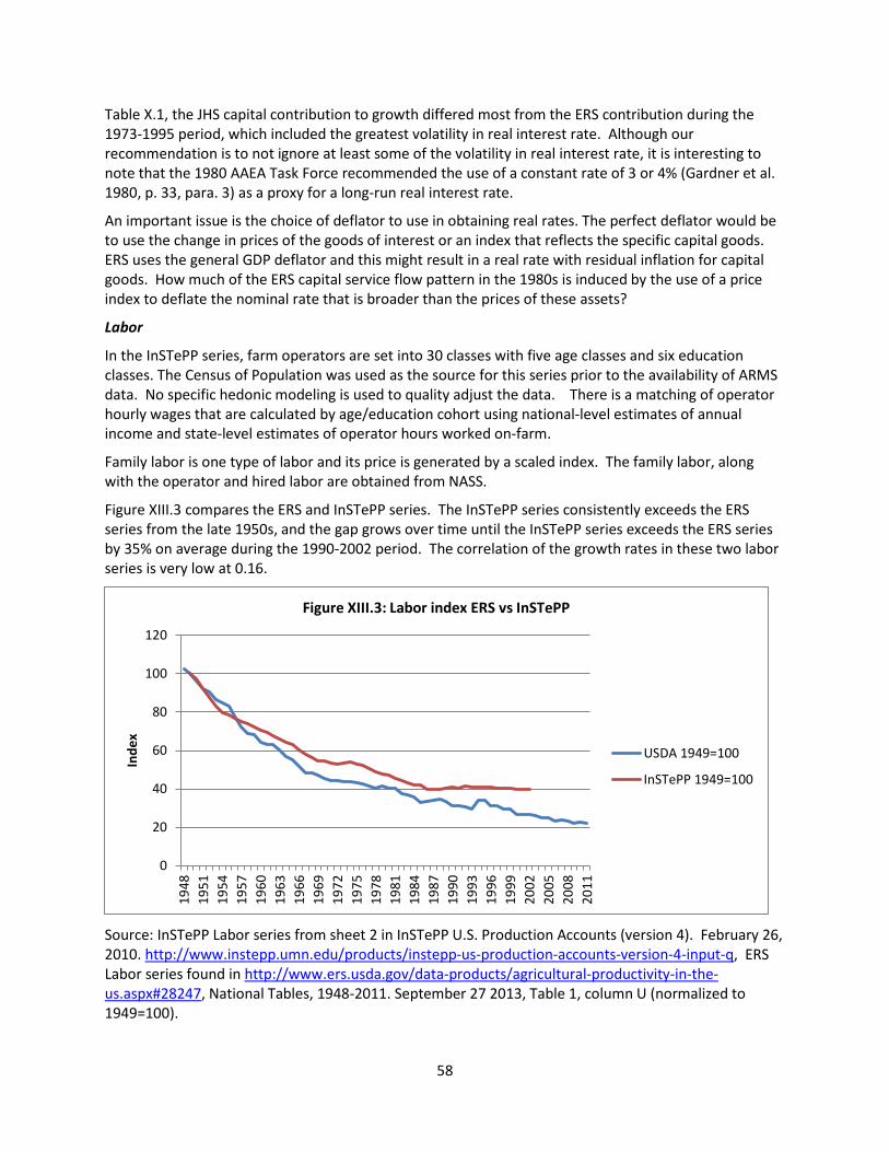
Table X.1, the JHS capital contribution to growth differed most from the ERS contribution during the 1973-1995 period, which included the greatest volatility in real interest rate. Although our recommendation is to not ignore at least some of the volatility in real interest rate, it is interesting to note that the 1980 AAEA Task Force recommended the use of a constant rate of 3 or 4% (Gardner et al. 1980, p. 33, para. 3) as a proxy for a long-run real interest rate.

An important issue is the choice of deflator to use in obtaining real rates. The perfect deflator would be to use the change in prices of the goods of interest or an index that reflects the specific capital goods. ERS uses the general GDP deflator and this might result in a real rate with residual inflation for capital goods. How much of the ERS capital service flow pattern in the 1980s is induced by the use of a price index to deflate the nominal rate that is broader than the prices of these assets?

Labor

In the InSTePP series, farm operators are set into 30 classes with five age classes and six education classes. The Census of Population was used as the source for this series prior to the availability of ARMS data. No specific hedonic modeling is used to quality adjust the data. There is a matching of operator hourly wages that are calculated by age/education cohort using national-level estimates of annual income and state-level estimates of operator hours worked on-farm.

Family labor is one type of labor and its price is generated by a scaled index. The family labor, along with the operator and hired labor are obtained from NASS.

Figure XIII.3 compares the ERS and InSTePP series. The InSTePP series consistently exceeds the ERS series from the late 1950s, and the gap grows over time until the InSTePP series exceeds the ERS series by 35% on average during the 1990-2002 period. The correlation of the growth rates in these two labor series is very low at 0.16.

Source: InSTePP Labor series from sheet 2 in InSTePP U.S. Production Accounts (version 4). February 26, 2010. http://www.instepp.umn.edu/products/instepp-us-production-accounts-version-4-input-q, ERS Labor series found in http://www.ers.usda.gov/data-products/agricultural-productivity-in-the-us.aspx#28247, National Tables, 1948-2011. September 27 2013, Table 1, column U (normalized to 1949=100).

0

20

40

60

80

100

120

1948

1951

1954

1957

1960

1963

1966

1969

1972

1975

1978

1981

1984

1987

1990

1993

1996

1999

2002

2005

2008

2011

Inde

x

Figure XIII.3: Labor index ERS vs InSTePP

USDA 1949=100

InSTePP 1949=100

58




Land

InSTePP notes ERS practice of using “land in farms” as a measure of the land input is problematic for the following reasons:

• Does not allow for consistent and economically meaningful treatment of cross-sectional, temporal variation in land quality, and

• Significantly mis-measures the actual number of acres in agriculture.

InSTePP attempts to measure acreage more accurately by building up from the state level using three land categories (cropland, irrigated cropland, and grassland and pasture). The InSTePP distinction is to separate grassland and pasture land from cropland. Further, state-level estimates of total irrigated acres for cropland and pasture land along with interpolations are used to generate the irrigated land series (Pardey, et al. 2006).

Land rental rates paid differ by agricultural land type. InSTePP uses information on rents from a state-level series as well as from two other reports (Daugherty 1989; Doll and Widdows 1982). When the data are insufficient to differentiate land rental rates between cropland and pastureland, and irrigated and non-irrigated land at the state level, one of six alternative methods is used to approximate state rental rates. They are then aggregated up to the national level.

Figure XIII.4 compares the ERS and InSTePP land series. The InSTePP series consistently exceeds the ERS series, and the gap widens over time. For the 1990-2002 period, the InSTePP series exceeds the ERS series by 27% on average. The correlation of the growth rates in these two land series is very low and negative, -0.09.

Source: InSTePP Land series from sheet 3 in InSTePP U.S. Production Accounts (version 4) (Pardey et al. 2010a. http://www.instepp.umn.edu/products/instepp-us-production-accounts-version-4-input-q, ERS Land series found in http://www.ers.usda.gov/data-products/agricultural-productivity-in-the-us.aspx#28247, National Tables, 1948-2011. September 27, 2013. Table 1, column S (normalized to 1949=100).

0

20

40

60

80

100

120

1948

1952

1956

1960

1964

1968

1972

1976

1980

1984

1988

1992

1996

2000

2004

2008

Inde

x

Figure XIII.4: Land Index ERS vs InSTePP

USDA 1949=100

InSTePP 1949=100

59




Materials

The materials input is comprised of fertilizer, pesticides, seed, purchased feed, water use, and other operating expenses which include machine hire. The challenge in creating the state series is that the collection of data for some inputs was discontinued during the time period. With the goal of developing state-level series uppermost in the InSTePP protocol, creative approaches to filling in these series were undertaken.

InSTePP made an effort to extend the separate fertilizer commodities by state after 1985, when the separation was discontinued. For fertilizer prices, national-level prices post 1988 were extrapolated using the trend in average prices of a) urea, b) triple superphosphate and c) muriate of potash/ potassium chloride, with the price data coming from Agricultural Prices (NASS publication).

Pesticides prices use ERS series with prices paid indexes from NASS. No quality adjustments are addressed. The seed series uses the total nominal expenditure of seed purchases by state in 1949-86 for seed used on farms. This series does not include seed grown and used on farm or purchased for resale. A national level price index is used. Purchased feed series use the nominal value of expenditures and total feed purchases by state for various types. The value of feed used on farm was not included but hay purchases were included even though consumed on farm. InSTePP generates the quantity index using the price of feed and they do this for 14 feed categories. Water use and other operating expenditures use the same data as ERS.

Figure XIII.5 compares the ERS and InSTePP materials series. The InSTePP begins to differ dramatically by the late 1950s with the gap growing dramatically. For the 1990-2002 period, the InSTePP series exceeds the ERS series by 21% on average. The correlation of the growth rates in these two materials/intermediate input series is 0.76.

Source: InSTePP Materials series from sheet 5 in InSTePP U.S. Production Accounts (version 4). February 26, 2010. http://www.instepp.umn.edu/products/instepp-us-production-accounts-version-4-input-q.

0

50

100

150

200

250

300

1949

1951

1953

1955

1957

1959

1961

1963

1965

1967

1969

1971

1973

1975

1977

1979

1981

1983

1985

1987

1989

1991

1993

1995

1997

1999

2001

2003

2005

2007

2009

2011

Figure XIII.5 Materials Index USDA vs InSTePP

USDA 1940=100

InSTePP 1949=100

60


ERS Intermediate goods series found in http://www.ers.usda.gov/data-products/agricultural-productivity-in-the-us.aspx#28247, National Tables, 1948-2011. September 27, 2013. Table 1, column X (normalized to 1949=100).

Output

Output quantity and price data are from NASS. They identify three categories – crops, livestock and miscellaneous. There are 60 crop outputs grouped into four categories – field crops (17), fruits and nuts (21), vegetables (21), and an aggregate nursery/greenhouse products; 9 livestock outputs – broilers, cattle, eggs, hogs, honey, milk, sheep, turkeys and wool; and a miscellaneous category with 5 components that includes machines rented out and Conservation Reserve acreage. Of the 74 outputs, 71 are based on both quantity and price data collected by national or state-level statistical services. Only 3 products (cattle, sheep, and machine hire out) generate a quantity series implicitly using revenue data and a price series.

Figure XIII.6 compares the ERS and InSTePP series. The InSTepp series coincides with the ERS series over the entire period, with a correlation of 0.999.

Source: InSTePP Output series from sheet 1 in InSTePP U.S. Production Accounts (version 4) – Output Q. Pardey et al., 2010b. http://www.instepp.umn.edu/products/instepp-us-production-accounts-version-4-output-q. ERS Aggregate Output Series found in http://www.ers.usda.gov/data-products/agricultural-

0

50

100

150

200

250

300

1949

1951

1953

1955

1957

1959

1961

1963

1965

1967

1969

1971

1973

1975

1977

1979

1981

1983

1985

1987

1989

1991

1993

1995

1997

1999

2001

2003

2005

2007

2009

2011

USDA 1949 = 100

InSTepp 1949 = 100

61



http://www.instepp.umn.edu/products/instepp-us-production-accounts-version-4-output-q

http://www.instepp.umn.edu/products/instepp-us-production-accounts-version-4-output-q


productivity-in-the-us.aspx#28247, National Tables, 1948-2011. September 27, 2013. Table 1, column B (normalized to 1949=100).

Total factor productivity

While the capital services series receives considerable attention in discussions concerning the discrepancies between the InSTePP and ERS series, the discrepancies other input series are not insignificant. Figure XIII.7 compares the ERS and InSTePP TFP series. The InSTePP series exceeds the ERS series from the outset, with the most dramatic differences emerging in the late 1970s to late 1980s, and then generally converging. For the 1990-2002 period, the InSTePP series exceeds the ERS series by 13%. The correlation of the growth rates in the TFP series is high at 0.94.

Source: InSTePP Multifactor Productivity Output series in InSTePP U.S. Production Accounts (version 4) – Multifactor Productivity. Pardey et al., 2010c. http://www.instepp.umn.edu/products/instepp-us-production-accounts-version-4-multifactor-productivity. ERS Series from found in http://www.ers.usda.gov/data-products/agricultural-productivity-in-the-us.aspx#28247, National Tables, 1948-2011. September 27, 2013. Table 1, column AE. (normalized to 1949=100).

Concluding comments

When comparing these series, nuanced differences emerge in the composition of the data in terms of levels of disaggregation and the use of state- or regional-level prices when available versus the national prices. By focusing on the state-level data series and matching highly disaggregated quantity series with their prices, the InSTePP series obviates some of the need for hedonic approaches that are used by ERS using national level data. An exception is the ERS land accounts which are not quality adjusted. Starting with the most disaggregated level possible can clearly be an advantage in data quality and consistency, but this necessitates high quality state-level data.

While there is considerable discussion about the difference between the InSTePP and ERS methodological differences in the capital series, controlling for use of the market versus constant interest leads to closer harmony between the ERS and InSTePP series. But not to be overlooked, the ERS and InSTePP series differ dramatically since the 1960s for labor, land, and materials.

0

50

100

150

200

250

300

1949

1951

1953

1955

1957

1959

1961

1963

1965

1967

1969

1971

1973

1975

1977

1979

1981

1983

1985

1987

1989

1991

1993

1995

1997

1999

2001

2003

2005

2007

2009

2011

Figure XIII.7: TFP Index ERS vs InSTePP

USDA 1949=100

InSTePP 1949=100

62


http://www.instepp.umn.edu/products/instepp-us-production-accounts-version-4-multifactor-productivity

http://www.instepp.umn.edu/products/instepp-us-production-accounts-version-4-multifactor-productivity


In the end, the TFP series for ERS and InSTePP tells a more harmonious story than any of the components separately.

Recommendation

Engage with researchers in the field to analyze the sources of differences with alternative estimates and to determine whether they warrant changes in data or procedures used (Priority B).

XIV. Stakeholder Assessment As part of the review process, the committee contacted stakeholders from academia, government, and the broader research community for comments on the productivity accounts. Overall, the comments were overwhelmingly supportive of the agricultural productivity accounts and repeatedly indicated the value of the accounts as analytical, research, and teaching tools. A common theme among stakeholder comments was requests for additional documentation, underlying source data, and for re-establishing the state-level accounts. The comments from stakeholders who granted permission to have their comments included verbatim are included in Appendix 2.

The call for stakeholder input was announced in the AAEA Newsletter and extended via direct email contact to representatives from both the agricultural economics community and the broader community of those doing productivity research. The committee received 33 responses. All but two have agreed to have their comments included verbatim in a supplemental appendix to this report. Three are included in Appendix 1 along with other input cited in this report. The remaining 28 are included in Appendix 2.

We divided the stakeholder responses into four categories: a) those expressing a complimentary view of the accounts, but offering no specific suggestions, b) those with feedback or requests related to the ERS productivity program, but no explicit critique or methodological suggestion, c) those with a specific critique or methodological concern, and d) those that offered no specific suggestion or critique or were not familiar enough with the program to offer feedback. It is important to note that those with a critique or methodological concern were often complimentary of the overall program.

Thirteen respondents offered specific suggestions or comments for the ERS productivity program but did not convey major methodological critiques. For example, respondents requested more documentation, more detailed and timely release of data, reinstatement of the state accounts, additional crop detail, coverage of aquaculture, and suggested that the ERS search for ways to make all of the data more visible. Within this group, respondents argued that measuring input quality is of utmost importance, questioned whether change in TFP should be zero if all inputs are accurately measured, and pointed out the potential differences between industry and firm-level TFP estimates. Furthermore, two respondents discussed choice of the residual claimant. As noted above, these respondents were often complimentary of the program overall.

Eight respondents offered a complimentary review of the ERS accounts without offering any specific suggestions for future directions. These respondents enumerated many reasons for their positive assessment of the accounts. In particular, stakeholders noted that ERS has been an international leader in productivity measurement and provides useful source data for international comparisons and policy work.

Four stakeholders responded with measurement or methodological issues related to the accounts. Within this group, respondents mentioned choice of index number formula, the consistency between the international and national agricultural accounts, the consistency in aggregation of productive stocks

63

and the formulation of the rental rate of capital, the inclusion of biological capital, and the measurement of agricultural land as important areas that deserve additional attention.

Eight respondents did not offer specific comments or suggestions.

64