sciences earth system hydrology and rainfall-runoff ... · pdf filehydrology and earth system...

Hydrology and Earth System Sciences, 9, 243–261, 2005www.copernicus.org/EGU/hess/hess/9/243/SRef-ID: 1607-7938/hess/2005-9-243European Geosciences Union

Hydrology andEarth System

Sciences

Rainfall-runoff modelling in a catchment with a complexgroundwater flow system: application of the RepresentativeElementary Watershed (REW) approach

G. P. Zhang and H. H. G. Savenije

Water Resources Section, Faculty of Civil Engineering and Applied Geosciences, Delft University of Technology, Stevinweg1, P.O. Box 5048, 2600 GA Delft, The Netherlands

Received: 7 March 2005 – Published in Hydrology and Earth System Sciences Discussions: 12 May 2005Revised: 11 August 2005 – Accepted: 2 September 2005 – Published: 21 September 2005

Abstract. Based on the Representative Elementary Water-shed (REW) approach, the modelling tool REWASH (Rep-resentative Elementary WAterShed Hydrology) has been de-veloped and applied to the Geer river basin. REWASH is de-terministic, semi-distributed, physically based and can be di-rectly applied to the watershed scale. In applying REWASH,the river basin is divided into a number of sub-watersheds, socalled REWs, according to the Strahler order of the river net-work. REWASH describes the dominant hydrological pro-cesses, i.e. subsurface flow in the unsaturated and saturateddomains, and overland flow by the saturation-excess andinfiltration-excess mechanisms. The coupling of surface andsubsurface flow processes in the numerical model is realisedby simultaneous computation of flux exchanges between sur-face and subsurface domains for each REW. REWASH is aparsimonious tool for modelling watershed hydrological re-sponse. However, it can be modified to include more com-ponents to simulate specific processes when applied to a spe-cific river basin where such processes are observed or con-sidered to be dominant. In this study, we have added a newcomponent to simulate interception using a simple paramet-ric approach. Interception plays an important role in the wa-ter balance of a watershed although it is often disregarded.In addition, a refinement for the transpiration in the unsat-urated zone has been made. Finally, an improved approachfor simulating saturation overland flow by relating the vari-able source area to both the topography and the groundwaterlevel is presented. The model has been calibrated and veri-fied using a 4-year data set, which has been split into two forcalibration and validation. The model performance has beenassessed by multi-criteria evaluation. This work represents

Correspondence to:G. P. Zhang([email protected])

a complete application of the REW approach to watershedrainfall-runoff modelling in a real watershed. The resultsdemonstrate that the REW approach provides an alternativeblueprint for physically based hydrological modelling.

1 Introduction

Hydrological models are important and necessary tools forwater and environmental resources management. Demandsfrom society on the predictive capabilities of such modelsare becoming higher and higher, leading to the need of en-hancing existing models and even of developing new the-ories. Existing hydrological models can be classified intothree types, namely, 1) empirical models (black-box mod-els); 2) conceptual models; and 3) physically based models.To address the question of how land use change and climatechange affect hydrological (e.g. floods) and environmental(e.g. water quality) functioning, the model needs to containan adequate description of the dominant physical processes.

Following the blueprint proposed by Freeze and Harlan(1969), a number of distributed and physically based modelshave been developed, among which are the well-known SHE(Abbott et al., 1986a, b), MIKE SHE (Refsgaard and Storm,1995), IHDM (Beven et al., 1987; Calver and Wood, 1995),and THALES (Grayson et al., 1992a) models. These modelsare able to produce variations in state-variables over spaceand time, and representations of internal flow processes. Itis assumed that the parameter values in the equations ofsuch models can be obtained from measurements as longas the models are used at the appropriate scale. Physically-based distributed models particularly aim at predicting theeffects of land-use change. However, considerable debate on

© 2005 Author(s). This work is licensed under a Creative Commons License.

244 G. P. Zhang and H. H. G. Savenije: Application of the REW approach in rainfall-runoff modelling

both the advantages and disadvantages of such models hasarisen along with research and applications of those mod-els (see, e.g. Beven 1989, 1996a, b, 2002; Grayson et al.,1992b; Refsgaard et al., 1996; O’Connell and Todini, 1996).In general, such models are very data-intensive and time-consuming when applied in a fully distributed manner. Inapplications, the model scale is generally much larger thanthe scale of parameter measurements. Therefore, “effective”parameter values have to be adopted in model applicationsand thus calibration becomes inevitable for physically basedmodels. This leads to the difficulty of parameter identifi-cation and the equifinality problem (Beven, 1993, 1996c;Savenije, 2001).

Conceptual models form by far the largest group of hydro-logical models that have been developed by the hydrologi-cal community and which are most often applied in opera-tional practice. Among those are SAC-SMA (Burnash et al.,1973; Burnash, 1995), HBV (Bergstrom and Forsman, 1973;Bergstrom, 1995), and LASCAM (Sivapalan et al., 1996).Most conceptual models are spatially lumped, neglecting thespatial variability of the state variables and parameters. Toimprove the potential for making use of spatially distributeddata, some lumped conceptual models have been extended tobe distributed or semi-distributed. Examples are the HBV-96model (Lindstrom et al., 1997), TOPMODEL (Beven, 1995)and the ARNO model (Todini, 1996). Parameters of this typeof models, however, either lack physical meaning or cannotbe measured in the field. Parameter identifiability and equi-finality are the major concerns of such models.

In view of all these different types of modelling ap-proaches, one can notice that there is no commonly acceptedgeneral framework for describing the hydrological responsedirectly applicable at watershed scale. To fill this gap, Reg-giani et al. (1998, 1999) made an attempt to derive a uni-fying framework for modelling watershed response, whichhas been named the Representative Elementary Watershed(REW) approach. This theory applies global balance lawsof mass and momentum and yields a system of coupled non-linear ordinary differential equations at the REW scale, gov-erning flows between different sub-domains of a REW. Todemonstrate the applicability of the REW approach, Reg-giani et al. (2000) investigated the long-term water balanceof a single hypothetical REW using the equations in non-dimensional form. In that work, only hill-slope subsurfaceresponses, i.e. flows in the unsaturated and saturated zoneswere considered. In succession, Reggiani et al. (2001) ap-plied the REW approach to a natural watershed but only fo-cusing on the response of the channel network. They pro-vided the theoretical development of the REW approach anddemonstrated that the approach can provide a framework foran alternative blueprint for modelling watershed response(Beven, 2002; Reggiani and Schellekens, 2003).

Parallel to theory formulation, much work has been doneto apply the REW approach towards the development of wa-tershed models. Zhang et al. (2003, 2004a, b, 2005a) and

Reggiani and Rientjes (2005) reported on advances of theresearch in this regard. However, as Beven (2002) pointedout while discussing about the REW approach, one shouldrecognise that the balance equations alone are indeterminate,and additional functional relationships associated with thesimplifying assumptions (i.e. the so called constitutive rela-tionships), for the fluxes within and between REWs, are cru-cial to the closure of the system. We would like to stressthis issue as the closure problem. Lee et al. (2005) andZehe et al. (2005) presented comprehensive discussions inthis regard. One can understand that developing closure re-lations is in fact the way of parameterisation. Thus, properclosure relations are keys to a successful application of theapproach. Zhang et al. (2005a) made a step towards a bet-ter model parameterisation and showed encouraging resultswhen applied to a temperate humid watershed. Meanwhile,it is obvious that an incomplete description of hydrologicalprocesses inevitably results in poor performance and leads toerroneous results. For instance, as pointed out by Savenije(2004, 2005), neglecting interception can introduce signifi-cant errors in other parameters. Moreover, previous researchon the REW approach to modelling of actual catchmentshighlighted the need for significant improvements. There-fore, this paper reports on the current state of developmentof the REW approach within our research framework.

In this work, the numerical model REWASH has been de-veloped based on the original code developed byP . Reg-giani and reflected in the application presented in Reggianiand Rientjes (2005). REWASH includes the process of in-terception and a modified transpiration scheme for the un-saturated zone. The model has been applied to the Geer riverbasin and the model performance has been evaluated throughcalibration and verification procedures. Model calibrationand verification have been carried out through a combinationof manual and automatic calibration, and a split-sample test.Sensitivity analysis has been performed to examine modelbehaviour and identify the most important parameters. Mod-elling results show that the hydrographs can be well repro-duced and the model is able to simulate the watershed re-sponse at a large spatial scale in a lumped fashion while theparameters are kept physically meaningful. However, thereis still considerable scope for improvement (e.g. Zhang etal., 2005b). It is realised that closure relations need to bewatershed-specific, depending on the dominant mechanismsand data availability.

2 Mathematical representation of the hydrological pro-cesses

2.1 The concept of the REW approach

In the REW approach, a river basin is spatially divided intoa number of sub-watersheds, so-called REWs. The REWpreserves the basic structure and functional components of

Hydrology and Earth System Sciences, 9, 243–261, 2005 www.copernicus.org/EGU/hess/hess/9/243/

G. P. Zhang and H. H. G. Savenije: Application of the REW approach in rainfall-runoff modelling 245

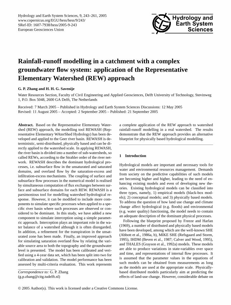
a watershed (hill-slopes and channels, Fig. 1). The discreti-sation is based on the analysis of the basin topography usingthe Strahler stream order system. The topographical bound-aries of REWs coincide with their surface water divides, thusREWs are naturally interconnected through the stream net-works as well as through the subsurface flow paths in termsof water flux exchanges. While determining the size of in-dividual REWs and their sub-domains, each REW is implic-itly defined in three dimensions and delimited externally bya prismatic mantle.

The volumetric entities of a REW contain flow domainscommonly encountered or described within a watershed: 1)the unsaturated flow domain, 2) the saturated flow domain,3) the saturation-excess overland flow domain, 4) the con-centrated overland flow domain (or the infiltration-excessoverland flow domain), and 5) the river channel. Hydrologi-cal processes in these domains are characterised by differenttemporal scales. For instance, overland flow has a time scaleof minutes to hours, while saturated groundwater flow hasmonths to years (Bloschl and Sivapalan, 1995).

In the REW approach, averaged balance equations of massand momentum for each flow domain were derived (Reggianiet al., 1998, 1999), resulting in a set of non-linear ordinarydifferential equations (ODEs) which no longer contain anyspatial information below the REW scale. In contrast to grid-based methods applied in most distributed model approaches(e.g. Abbott et al., 1986a, b), the REW approach uses thesub-watersheds (REWs) as “cells”, the basic discretisationunits on which the ODEs are solved.

The general form of the ODEs reads:

dφ

dt=

∑i

eφi + s (1)

whereφ represents a generic thermodynamic property suchas mass or momentum.eφi stands for a generic exchangeterm of φ and s is a grouped sink/source term for the do-main in question. This form can be extended to include termsfor more complex flow phenomena, such as multi-phase flowand pollutants transport. As we know, the conservation equa-tion itself alone is not a closed system. The exchange termeφi is unknown and needs to be specified. This term has to beexpressed in a form that relates the state variables to other re-solved variables. This comes to the problem of finding properclosure relations for the balance equations, as touched uponin the introduction. Closure relations for process descrip-tions at the catchment-scale, other than the point-scale or theREV (representative elementary volume) scale, are not read-ily available. However, after rigorous theoretical derivation,REW-scale equations for: Darcy’s law, Manning’s law, andthe Saint-Venant equations have been obtained and employedin our model, which are valid for subsurface, overland andchannel flow, respectively. The relations of these equationsto the flux terms are summarised in Table 1 of the followingsection.

Outflow

Atmosphere

Saturation-excess

overland flow domain

Unsaturated

flow domain

Channel reach

Saturated

flow domain

Infiltration-excess

overland flow domain

Fig. 1. A 3-D view of the volume comprising a single REW (modi-fied from Reggiani and Schellekens, 2003).

2.2 Description of the numerical model

In many hydrological models or model approaches, intercep-tion is neglected even though it is the first process in the chainof interlinked rainfall-runoff processes (Savenije, 2004). Byignoring this process, errors are introduced that propagateinto the subsequent processes simulated (particularly into thesoil moisture and groundwater flow process) and into the wa-ter balance regime in the different stores of a watershed, al-though sometimes they may not be detected by only lookingat the single integral output: the simulated stream discharge.In the initial stage of the development and application ofthe REW approach, interception was not explicitly consid-ered. Bearing this in mind, we have added a component inthis model using a simple parametric approach to account forthe interception effect. In addition, in line with the work byZhang et al. (2003, 2004a, b), a refinement for sub-grid vari-ability of soil properties in the soil column has been takeninto account. Moreover, a new approach to determine thesaturated overland area has been introduced. Based on thesemodifications, the water balance equations for the differentflow domains and governing equations for the various flowprocesses are described below.

2.2.1 Water balance equations for flow domains

Mass conservation is the first principle ruling water flux ex-changes in a watershed system. In accordance with observa-tion and understanding of the flow processes in the terrestrialsystem, a REW is sub-discretised vertically into various flowdomains. Figure 2 illustrates the schematised profile of aREW with the different flow domains, their geometric quan-tities and the water flux exchange terms. With reference toFig. 2, the water balance equations for each flow domain aregiven as follows.

www.copernicus.org/EGU/hess/hess/9/243/ Hydrology and Earth System Sciences, 9, 243–261, 2005


Average ground surface

Average bottom

Average g.w. table

Datum

zs

zr

ys

zsu

rf

yu

γo

Average river bed

ecu

eus

eua

Szone

UzoneCzone

Ozoneeso

esr

River

eor

eoa

esi

ectop

eotopertop era

eca

Fig. 2. Schematised cross-sectional profile of a REW. Czone,Ozone, Uzone, Szone and River stand for the infiltration-excessoverland flow domain, the saturation-excess overland flow domain,the unsaturated flow domain, the saturated flow domain and theRiver flow domain, respectively.ectop, ecu, eca etc. are flux terms.yu, ys are stock variables, andzs , zr , zsurf andγo are average ge-ometric quantities of the REW.

Infiltration-excess overland flow domain

dSc

dt= ectop + eca + ecu + eco (2)

whereSc (M) is the storage of the infiltration-excess over-land flow domain. The fluxesectop (MT−1), eca (MT−1),ecu (MT−1) andeco (MT−1) are the rainfall on the surface ofthis zone, the evaporation from interception on this zone, theinfiltration to the saturated zone and the transfer towards thesaturation-excess flow domain, respectively. Since we are ap-plying this model approach to a humid temperate river basinwhere the saturation-excess flow is dominant, the infiltration-excess overland flow is negligible, thuseco is kept zero.

Saturation excess overland flow domain

dSo

dt= eotop + eoa + eos + eor + eoc (3)

whereSo (M) is the storage of the saturation-excess over-land flow domain. The fluxeseotop (MT−1), eoa (MT−1), eos(MT−1), eor (MT−1) andeoc (MT−1) are the rainfall on thesurface of this zone, the evaporation from this zone, the ex-change between this zone and the saturated flow zone, thetransfer to the river channel, and the exchange between thiszone and the infiltration-excess flow zone, respectively. Forthe same reason stated above,eoc is ignored.

Unsaturated subsurface flow domain

dSu

dt= eua + euc + eus (4)

whereSu (M) is the storage of the unsaturated flow domain.The fluxeseua (MT−1), euc (MT−1), andeus (MT−1) are thetranspiration, the infiltration and the percolation.

Saturated subsurface flow domain

dSs

dt= esu + eso + esr + esi + esa (5)

whereSs (M) is the storage of the saturated flow domain. Thefluxes esu (MT−1) and eso (MT−1) are the counterparts ofeus (MT−1) andeos(MT−1) in Eqs. (3) and (4), respectively;esr (MT−1), esi (MT−1) andesa (MT−1) are the exchangebetween the saturated zone and river channel, the exchangewith the neighbouring REWs (if any) and the groundwaterabstraction (if any).

River channel

dSr

dt= ertop + era + ers + ero + erin + erout (6)

whereSr (M) is the storage of the river channel segmentwithin the REW under investigation. The fluxesertop(MT−1), era (MT−1), erin (MT−1) anderout (MT−1) are therainfall on the channel water surface, the evaporation fromthe water surface, the water coming from upstream channelsegment(s) and the flow out of the segment of the REW inquestion, respectively. The fluxesers (MT−1), ero (MT−1)are the counterparts ofesr andeor in Eqs. (3) and (5), respec-tively.

The functional relationships to quantify the flux terms pre-sented in these equations are described in the following sec-tion.

2.2.2 Parameterised governing equations for rainfall-runoffprocesses

Rainfall input

The rainfall flux on a REW is partitioned into three por-tions in terms of the area that captures the rainfall, whichareectop,the rainfall flux to the infiltration-excess overlandflow area,eotop to the saturation overland flow area andertopto the river channel, respectively. They are described by ectop = ρiAωceotop = ρiAωoertop = ρilrwr

(7)

whereρ (ML−3) is the water density;A (L2) the horizontallyprojected surface area of the REW;i [LT−1] the precipitationintensity.ωc (–) andωo (–) are the infiltration-excess and thesaturation-excess overland flow area fractions, respectively.lr (L) andwr (L) are the length and the average width of thechannel.

Interception

For modelling the detailed dynamics of the interception pro-cess, a complex descriptor derived from mass and energy



balance principles would be necessary. In that case, an ad-ditional model domain describing the process would be de-sirable and additional parameters such as the leaf area index(LAI) would be required. To keep the model as parsimoniousas possible, we chose a simple approach. We assume thatinterception is taking place in the infiltration-excess flow do-main. Considering a storage capacity of the interception me-dia (e.g. tree leaves, undergrowth, forest floor and surface)and assuming that the intercepted water will be eventuallyevaporated within a day, the interception flux is determinedby

eca = min(i, idc) ρAωc (8)

whereidc (LT−1) is the daily interception threshold.

Infiltration

Similar to the approach of Reggiani et al. (2000), the infiltra-tion capacity can be computed by

f =Ksu

3u

(1

2yu + hc

)(9)

wheref (LT−1) is the infiltration capacity;Ksu (LT−1) thevertical saturated hydraulic conductivity of the unsaturatedzone; 3u (L) the length over which the wetting front isreached;yu (L) the averaged unsaturated zone depth; andhc[L] the capillary pressure head,which is described using theBrooks and Corey (1964) soil water retention model:

hc = ψb

(θu

εu

)−1/µ(10)

whereψb (L) is the air entry pressure head;θu (–) andεu (–)are the soil moisture content and the effective soil porosity ofthe unsaturated zone, respectively;µ (–) is the soil pore sizedistribution index.

It is reasonable to assume that all rainfall reaching theground surface infiltrates into the soil when it is climate con-trolled, i.e. the rainfall intensity is lower than the infiltrationcapacity. Consequently, the actual infiltration flux is esti-mated by

ecu = min[(i − idc) , f ] ρωcA (11)

whereωc (–) is the area fraction of the infiltration-excessoverland flow zone, which is equal to the unsaturated zonearea fraction. The remaining symbols are the same as inthe above equations. The first term of the right-hand sidein Eq. (11) calculates the effective rainfall intensity.

Evaporation/transpiration

eua = min[1.0,

(2θuεu

)] [ep − min(i, idc)

]ρωuA (for Uzone)

eoa = epρωoA(for Ozone)

era = epρlrwr (for Rzone)

(12)

whereep (LT−1) is the potential evaporation. One can seethat when the soil moisture of the unsaturated zone is lessthan 50% of the soil porosity, it is assumed that the evapora-tion from the unsaturated zone is water constrained, leadingto a reduced evaporation rate. A linear reduction function isused here, which agrees with the procedure generally usedin agricultural engineering (e.g. Rijtema and Aboukhaled,1975; Doorenbos and Kassam, 1979).

Percolation/capillary rise

eus = αusρωcAKu

yu

[(1

2−θu

εu

)yu + hc

](13)

whereαus (–) is the scaling factor for this flux exchange term.Ku (LT−1) is the effective hydraulic conductivity for the un-saturated zone, which is a function of the saturation (θu/εu)of the unsaturated zone. As an additional condition, perco-lation is set to take place only ifθu is greater than the fieldcapacityθf . Ku can be determined by the following relation-ship in Brooks and Corey (1964) approach:

Ku = Ksu

(θu

εu

)λ(14)

λ = 3 +2

µ(15)

whereλ is the soil pore-disconnectedness index.

Base flow

esr =ρKsr lrPr

3r(hr − hs) (16)

whereKsr (LT−1) andPr (L) are the hydraulic conductivityfor the river bed transition zone and the wetted perimeter ofthe river cross section, respectively.3r (L) is the depth oftransition layer of the river bed.hr (L) and hs (L) are thetotal hydraulic heads in the river channel and the saturatedzone, respectively.

Exfiltration to the surface

eso =ρKssωoA

3s cosγo(hs − ho) (17)



whereKss (LT−1) andωo (–) are the saturated hydraulic con-ductivity for the saturated zone and the area fraction of thesaturated overland flow zone, respectively.hs (L) andho (L)are respectively the total hydraulic head in the saturated zoneand the saturated overland flow zone.3s (L) is a typicallength over which the head difference between the saturatedzone and the saturated overland zone is dissipated.γ o is theaverage slope angle of the seepage face in radian.

Regional groundwater flow

esi = αsiρ (hs − hsi) (18)

whereesi is the flux exchange between the saturated zonesof the REW in question and itsith neighbouring REW;hs(L) and hsi (L) are the total hydraulic heads of the satu-rated zones of the two neighbouring REWs, respectively.αsi (L2T−1) is a lumped scaling factor involving the contourlength of the mantle segment of theith REW, the harmonicmean of the saturated hydraulic conductivity over the twoREWs, etc. If there is no groundwater connection betweenREWs or if the groundwater level has a horizontal gradientat the water divide, thenαsi is set to zero.

Lateral overland flow to channel

eor = 2ρyolr1

n(sinγo)

1/2 (yo)2/3 (19)

whereyo (L) is the average depth of the flow sheet on the sur-face of the overland flow domain; andn (TL−1/3) the Man-ning roughness coefficient.

Channel flow

erin = ρ∑i

1

2mri (vr + vri) (20)

erout = ρ1

2mr

(vr + vrj

)(21)

vr =√√√√ 8g

Pr lrξ

[mr lrsinγr+

∑i

1

4yr (mr+mri)−

1

4yr

(mr+mrj

)](22)

wheremr (L2),mri (L2) andmrj (L2) are the average cross-sectional area of the channel segment under study, of theith inflow channel and of the outflow channel, respectively;vr (LT−1), vri (LT−1) and vrj (LT−1) are the flow veloci-ties within the channel segment under study, and of the in-flow and outflow channels, respectively;ξ (–) is the averageDarcy-Weisbach friction factor andg (LT−2) is the gravita-tional acceleration;γ r (–) is the average slope angle of theriver channel andyr (L) is the water depth of the channelunder study.

To summarise the parameterisation of the mass balanceequations, Table 1 provides a clear presentation of the fluxterms and their closure functions.

2.2.3 Additional functional relationships for the closure ofthe water balance equations

Zhang et al. (2004b, 2005a) proposed an expression for thesaturation overland flow area fraction, which has the follow-ing form:{ωo = αsf

(ys+zs−zrzsurf−zr

)tanγo(if ys + zs ≥ zr)

ωo = 0 (if ys + zs < zr)(23)

Therefore,

dωo

dt= αsf

(ys + zs − zr)tanγo−1(

zsurf − zr)tanγo

tanγodys

dt

(if ys + zs ≥ zr) (24)

whereαsf (–) is a scaling factor, which can be estimatedfrom the surface runoff coefficient taking into account theaverage groundwater level.ys, zs, zr , zsurf andγ o are thegeometric quantities of a REW defined in Fig. 2.

There are a number of geometric relationships supplemen-tary to the balance equations, among those:

ωo + ωc = 1 (25)

yuωc + ys = Z (26)

whereZ is the average soil depth of a REW. As a result,

dωc

dt= −

dωo

dt(27)

d

dt(yuωc) = −

dys

dt(28)

In Eq. (5), esa is the sink (groundwater abstraction) or source(artificial recharge) term, which can be calculated by

esa = ρGA (29)

whereG (LT−1) is the abstraction or recharge rate imposedon the REW in question.

Substituting Eqs. (7), (8), (9), (10), (11), (12), (13), (16),(17), (18), (19), (20), (21), (27), (28) and (29) into Eqs. (2),(3), (4), (5) and (6), we obtain the full water balance equa-tions for a REW.dyc

dt= i︸︷︷︸

rainfall

− min(i, idc)︸︷︷︸interception

−

min

[(i − idc) ,

Ksu

3u

(1

2yu + hc

)]︸︷︷︸

infiltraion

+yc

1 − ωo

dωo

dt︸︷︷︸area change

(30)

dyo

dt= i︸︷︷︸

rainfall

− ep︸︷︷︸evaporation

+Kss

3s cosγo(hs − ho)︸︷︷︸

groundwater exfiltration

−2yolrAωo

1

n(sinγo)

1/2 (yo)2/3︸︷︷︸

overland flow to channel

−yo

ωo

dωo

dt︸︷︷︸area change

(31)



Table 1. Flow processes, the flux terms and the closure relations.

Processes Flux terms Closure relations

Infiltration ecu min[(i − idc),

Ksu3u

(12yu + hc

)]ρAωu

(Darcy-type equation)

Percolation/Capillary rise

eus αusρωcAKuyu

[(12 −

θuεu

)yu + hc

](Darcy-type equation)

Overland flow eor 2ρyolr 1n (sinγo)1/2 (yo)2/3

(Manning’s equation)

Exfiltration to surface esoρKssωoA3s cosγo

(hs − ho)


Channel flow erin/erout ρ∑i

12mri (vr + vri)

ρ 12mr

(vr + vrj

)vr =

√√√√ 8gPr lr ξ

[mr lr sinγr +

∑i

14yr (mr +mri)−

14yr

(mr +mrj

)](simplified Saint-Venant Equation)

Base flow esrρKsr lrPr3r

(hr − hs)


Inter-REW groundwater flow esi αsiρ (hs − hsi)


dθu

dt= min

[(i − idc)

yu,Ksu

yu3u

(1

2yu + hc

)]︸︷︷︸

infiltration

−

min

(1.0,

2θuεu

) [ep − min(i, idc)

]yu︸︷︷︸

transpiration

−αusKu

y2u

[(1

2−θu

εu

)yu + hc

]︸︷︷︸

percolation/capillary rise

+θu

yuωu

dys

dt︸︷︷︸water table change

(32)

dys

dt=αusKuωc

εsyu

[(1

2−θu

εu

)yu + hc

]︸︷︷︸

percolation/capillary rise

−

Kssωo

εs3s cosγo(hs − ho)︸︷︷︸

groundwater exfiltration

−Ksr lrPr

Aεs3r(hs − hr)︸︷︷︸

base flow

−αsi

Aεs(hs − hsi)︸︷︷︸

regional groundwater flow

−G

εs︸︷︷︸sink/source

(33)

dm

dt= iwr︸︷︷︸

rainfall

− epwr︸︷︷︸evaporation

+KsrPr

3r(hs − hr)︸︷︷︸

base flow

+

2yo1

n(sinγo)

1/2 (yo)2/3︸︷︷︸

lateral flow from sat. overland flow area

+

∑i

1

2lrmi (vr + vri)︸︷︷︸

channel inflow

−1

2lrm

(vr + vrj

)︸︷︷︸channel outflow

(34)

These five equations, supplemented with geometric relations,form the mathematical core of the REWASH model code.For the solution of this system of equations, an adaptive-step-size controlled Runge-Kutta algorithm presented by Press etal. (1992) has been adopted. This algorithm, using the Cashand Karp (1990) approach, limits the local truncation error atevery time step to achieve a higher accuracy and robustnessof the solution scheme.

2.2.4 Treatment of sub-grid variability of soil propertieswithin a REW

Since Beven (1984) showed that there is decay in hydraulicconductivity with soil depth and Kirkby (1997) discussed theform of porosity decay, we have applied a division of the soilcolumn to take into account the sub-grid variability of soil



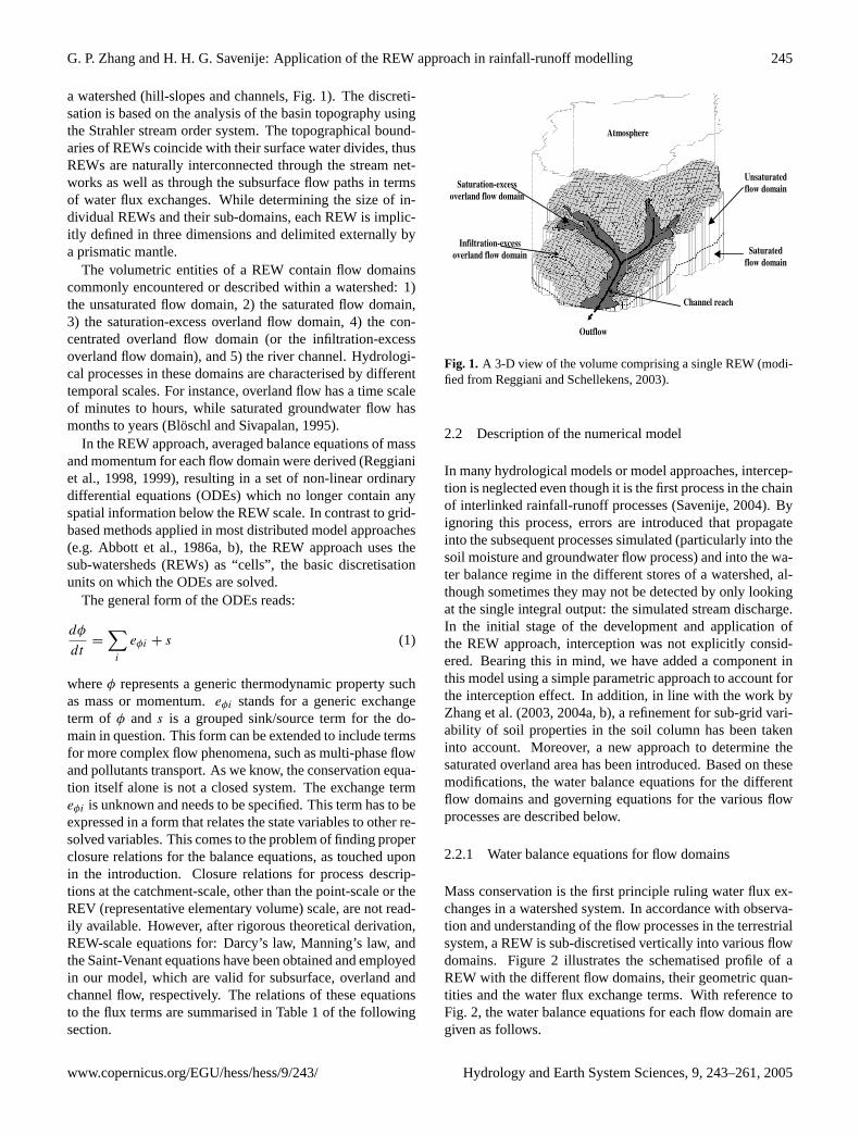
Fig. 3. Location of the Geer river basin and the Geer river network.

properties. In the real world, the variability of soil proper-ties is one of the factors that induce quick subsurface stormflow. Within a REW, the soil column is divided into two lay-ers. The average porosity and saturated hydraulic conductiv-ity of the upper layer are larger than those of the lower layer.It should be pointed out that this division of the soil pro-file does not necessarily coincide with the boundary betweenthe unsaturated and saturated zones as the consequence ofvarying water table depth. Therefore, the effective porosityof these two zones should be updated in time. Applying adepth-weighted averaging method, the effective porosity ofboth subsurface zones are given by:{εu =

[ε′udup + ε′s

(yu − dup

)]/yu (if yu > dup)

εu = ε′u (if yu ≤ dup)(35)

εs =[ε′u

(dup − yu

)+ ε′s

(zsurf − zr − dup

)]/(zsurf − zr − dup

)(if yu < dup)

εs = ε′s (if yu ≥ dup)

(36)

whereε′u (–) andε′s (–) are the soil porosity of the upper layerand the lower layer of the soil column, respectively;dup (L)is the depth of the upper soil layer. By this parameterisa-tion, in combination with the field capacity threshold, whichcontrols when percolation takes place, the time scales of theflow processes in the two subsurface domains can be betterrepresented.

3 Model application

3.1 Site description

The Geer river basin has been selected for this study. TheGeer river is a tributary of the Meuse River, located in Bel-gium (Fig. 3). The drainage area covers about 490 km2. Thebasin is characterised by a deep groundwater system, whichis delimited at the southern end by a ridge separating it from

the Meuse River. The substrata are made up by several lay-ers of chalk stone with low permeability. The groundwa-ter aquifer of the basin consists of Cretaceous chalks with athickness ranging from a few meters in the south to about100 m in the north. The aquifer is underlain by a layerof Smectite, which can be regarded as an impervious bot-tom boundary. The unsaturated zone above the aquifer canbe up to 40 m. The groundwater catchment does not cor-respond to the surface hydrological divide and extends be-yond the catchment boundaries, thus water most likely flowsacross the northern topographical divide. Moreover, there isgroundwater abstraction from wells and there are drainagegalleries in the basin. Spatial data, a DEM with 30 m×30 mresolution, as well as four years (1 January 1993–31 De-cember 1996) of daily rainfall, potential evaporation and dis-charges at the outlet are available.

3.2 Model calibration and sensitivity analysis

Model calibration is a procedure to adjust parameter valuesto achieve an optimal fit of model output to the correspond-ing measurements according to predefined objective func-tion(s) and performance measure(s). It involves model per-formance evaluation, which is to analyse the closeness ofmodel behaviour to the behaviour of the real world (Wa-gener, 2003). In General, objective function(s) and perfor-mance measure(s) are chosen, often subjectively, dependingon the purpose of the model application and issues to be in-vestigated. The approach used for calibration here is a com-bination of manual and automatic calibration strategy. Nash-Sutcliffe efficiency (R2

NS , Nash and Sutcliffe, 1970) and thepercentage bias (δB) are used for evaluating model perfor-mance. Since the goal of this work is not to pursue a bestmodel (or to find a best parameter set) but to show how aREW approach based model can be applied to in a real worldcatchment, we chose a level of 0.6 forR2

NS as the thresholdto discriminate a behavioural and non-behavioural model.



3.2.1 Parameter assignment and manual calibration

The river basin has been discretised into a finite number ofsub-watersheds, i.e. REWs, and the river network linkingeach REW has been generated using the modified versionof TARDEM (Tarboton, 1997). A second order threshold onthe Strahler river order system (Strahler, 1957) resulted in73 REWs (see Fig. 4). The parameters of the model consistof the interception threshold, surface roughness and channelfriction factor, soil properties and hydraulic characteristics.All these parameters are effective values at REW-scale. Ow-ing to the lack of spatially distributed information of theseparameters as well as some of the geometric properties, suchas the average total soil depth, the depth of the upper soillayer, and the river bed transition layer depth, we assume thatthey are uniformly distributed over the entire river basin. Theinitial state of the river basin is also assumed spatially uni-form. As a result, the model functions as a lumped model.On the other hand, it decreases the model parameters to amore manageable number and reduces drastically the cali-bration task, making a quick evaluation of the model at theearly development stage possible. For the derivation of initialestimates of soil parameters, we made a realistic guess basedon published values (e.g. Troch et al., 1993). Rainfall andpotential evaporation (based on Penman-Monteith equation)data, measured at Bierset gauging station (Fig. 4) from 1 Jan-uary 1993 to 31 December 1994 were used in simulation runsfor calibration. Discharge data, measured at the outlet of thecatchment in the same period were used for calibration. Theremaining two years of data were used for verification run.No data measured at interior flow gauges was available. Ithas been observed that the 4-year of data available for thisstudy cover both wet and dry periods, high and low flows.Further, no drastic changes in climate and land use, whichcould lead to changes of catchment rainfall runoff relations,have been documented. Therefore, the quantity and qualityof the data applied in this case is justified.

Knowing that water flows across the northern divide of theriver basin, we imposed a flux boundary condition for thoseREWs bordering the northern divide (REW12, REW13,REW25, REW26, REW27, REW52, REW69 and REW73).With respect to groundwater abstractions, sink terms havebeen synthesised as monthly time series on the basis of avail-able data and introduced to the saturated zone mass balanceequation for each REW. In addition, groundwater flow inter-actions between neighbouring REWs are considered explic-itly computed with Eq. (18).

It has appeared that the model needs around half a yearof run time for model initialisation (warming-up). We there-fore run the model using the time series for one year to reacha quasi dynamic equilibrium state. Subsequently we usedthis state as the initial state for model calibration so thatthe warming-up effect can be reduced to a negligible level.By applying a trial-and-error method, expert knowledge hasbeen used to identify parameter values. During manual cali-

12

2

3915 24

1

41

4862

46

73

38 5033

43

4

535

55

6

35

5929

44 49

3

54

3237

40

4534

36

70

61

22

71

21

69

13

47

2563

16

72

60

51

56

67

7

18

42

23

52

27

58

17

66

64658

19

68

57

31

10

2628

20

REWs of GEER Basin (2nd order)

Bierset

Fig. 4. Discretisation of the Geer river basin and the resultantREWs.

bration, the most sensitive parameters have been recognisedand physically meaningful ranges for those parameters deter-mined. In calibration, two constants, namely the scaling fac-tors,αus andαsf in Eq. (13) and Eq. (23), respectively, werenot subject to adjustment. In Eq. (13), αus is the scaling fac-tor resulted from linearisation of the dependent function ofthe mass exchange between the unsaturated domain and thesaturated domain (Reggiani et al., 2000). In this study, sim-ilar to Reggiani et al. (2000), we used the unsaturated soilporosity forαus , implying that the flow (recharge/capillaryrise flux) is conducting only through soil pores. As describedin Zhang et al. (2005a),ωo being a function of groundwaterlevel and surface slope, acts, in fact, as a surface runoff coef-ficient. With regard toαsf , we observe that in the right handside of from Eq. (23), the entire term within the brackets andits exponent vary between 0 and 1. Therefore,αsf shouldnot be larger than the catchment runoff coefficient. For a firstestimation ofαsf , the runoff coefficient, and preferably, thesurface runoff coefficient can be assigned.

During calibration, priority was given to fitting low flows.While visually inspecting the goodness of fit (comparisonof the simulated hydrograph against the observed), objectivemeasures such as the Nash-Sutcliffe efficiency (R2

NS , Nashand Sutcliffe, 1970), the percentage bias (δB) have been usedto evaluate the fit. The definition ofR2

NSandδB are given asfollows:

R2NS = 1.0 −

n∑i=1

(Qsi −Qoi)2

n∑i=1

(Qoi − Qo

)2(37)



δB =

∣∣∣∣∣∣∣∣n∑i=1

(Qsi −Qoi)

n∑i=1

Qoi

∣∣∣∣∣∣∣∣ × 100% (38)

whereQsi , Qoi andQo are the simulated discharge, the ob-served discharge at the time stepi and the mean of the ob-served discharge, respectively.δB represents the differenceof the total volume between the simulated and observed timeseries. The bias is an important measure to evaluate simula-tion of continuous models.

To give more information on how the model simulates thestream flow in different flow ranges, average relative errors(δp) were calculated.δp is expressed as

δp =1

n

n∑i=1

(|Qsi −Qoi |

Qoi

× 100%

)(39)

whereQsi andQoi are the same as in previous equations.

3.2.2 Sensitivity analysis

Sensitivity analysis (SA) is a useful tool to assess the effect ofparameter perturbations on model output. Many techniquesfor SA are available and they can be categorised into threegroups (see e.g. Saltelli, 2000): 1) factor screening, 2) localSA, and 3) global SA (often applied as regional sensitivityanalysis, RSA, in rainfall-runoff applications). The Fourieramplitude sensitivity test (FAST) and Monte Carlo simula-tion based methods (e.g. Hornberger and Spear, 1981; Bevenand Binly, 1992; Freer et al., 1996) are among the popularRSA approaches, which found their applications mostly forconceptual rainfall-runoff models. Apparently, local SA ap-proaches don’t take into account the effect of parameter in-teractions. RSA approaches implicitly account for the pa-rameter interaction effect and can explore a higher dimen-sional parameter space. However, few reports in rainfall-runoff modelling have explicitly discussed the effect of pa-rameter interactions on the parameter indentifiability. In fact,as Bastidas et al. (1999) and Wagener et al. (2004) pointedout, most SA approaches are weak in dealing with the is-sue of parameter interdependency. On the other hand, dueto the “curse of dimensionality” (Brun et al., 2001) and pro-hibitively high computational demand, RSA approaches arenot widely applied yet to large complex models. Instead,local approaches are often used (e.g. Senarath et al., 2000;Newham et al., 2003).

We used the one-at-a-time perturbation approach to pre-liminarily investigate the effect of parameter variation on themodel output that assists in gaining insight into model be-haviour, although sensitivity analysis is not the main goal ofthis work. This approach can be regarded as an expansionof factor screening that is helpful to filter out most impor-tant factors affecting model response. In this study, startingwith the manual calibration, each parameter has been varied

by +50% and−50% while the other parameters were main-tained unchanged. Having gained a knowledge of which pa-rameters are most sensitive in manual calibration, we chosesix parameters (idc, Ksu, Kss , ε′s , ε

′u, λ) to further evalu-

ate model sensitivity. Using the relative change in runoffvolume (δV ) and the relative change in Nash-Sutcliffe effi-ciency (δNS) as indices, the effect of each parameter changeon the runoff-producing events during the period from 1 Jan-uary 1993 to 31 December 1993 has been analysed.δV andδNS are defined as follows:

δV =

∣∣∣∣∣∣∣∣n∑i=1

(Qi+ −Qi−)

n∑i=1

Qim

∣∣∣∣∣∣∣∣ × 100% (40)

whereQi+,Qi− andQim refer to the discharges at the timestepi with the parameter value varied by +50%,−50% andthe manually calibrated parameter value, respectively. Thelarger theδV , the more sensitive the model is to the parameterunder study.

δNS =

∣∣∣∣∣R2NS+

− R2NS−

R2NSm

∣∣∣∣∣ × 100% (41)

whereR2NS+

, R2NS−

and R2NSm are the Nash-Sutcliffe effi-

ciency values with the parameter value varied by +50%,−50% and the manually calibrated parameter value, respec-tively. Same asδV , the larger theδNS , the more sensitive themodel to the parameter under study.

3.2.3 Automated parameter optimisation

A hybrid approach combining manual and automated cal-ibration methods is increasingly recognised as a more ef-fective way of parameter optimisation (Boyle et al., 2000).Boyle et al. (2000) first carried out automatic calibration us-ing the MOCOM-UA algorithm to obtain the Pareto solu-tion space and then selected one or more acceptable param-eter sets within the Pareto space through manual calibration.Obviously this calibration strategy has the advantage that agroup of good parameter sets can be efficiently filtered outby the automatic step. In our case, however, the model isnewly built and further development is still underway. Thus,an open-eyes manual calibration is a desirable way of gain-ing knowledge of model behaviour. Moreover, the modelis physically based so that parameters should be calibratedwithin physically reasonable ranges, which have to be de-fined before an automatic calibration step. Therefore, wecarried out manual calibration in the first step followed byautomatic calibration.

Following the trial-and-error procedure, we carried out anautomatic calibration procedure to enhance the accuracy ofthe model optimisation. During the manual calibration, phys-ically reasonable ranges of parameter values have been delin-eated. These ranges were then prescribed in the automatic



Table 2. The accepted best parameter values for the calibration period and the model performance.

Parameters idc(mm/d)

n

(s/m1/3)Kss(m/d)

Ksu(m/d)

Ksr(m/d)

ε′s(–)

ε′u(–)

λ

(–)θf(–)

Value 1.36 0.020 0.0097 0.0213 2.64 0.148 0.43 4.43 0.08R2NS

0.71δB 0.76%

calibration procedure for the fine adjustment of parametervalues. In this work, the optimisation tool GLOBE (Solo-matine, 1995, 1998) has been coupled to REWASH. GLOBEis a global optimisation tool consisting of a number of searchalgorithms: controlled random search (CRS2, CRS4); ge-netic algorithm (GA); adaptive cluster covering (ACCO),and with local search (ACCOL); multistart methods (e.g. M-simplex) etc. We choose the M-simplex algorithm for ourstudy, though Sorooshian et al. (1993) discussed that the M-simplex algorithm is not as efficient and effective as the shuf-fled complex evolution algorithm. In our modelling exer-cises, we also have tried different algorithms (GA, ACCOL).However, the accuracy gained was marginal and the com-putational efficiency was found lower than that with the M-simplex. Figure 5 shows the loop of the automated calibra-tion procedure. Pobj and Pupdate are the two programmeslinking REWASH to GLOBE. These programmes are drivenby GLOBE in each evaluation loop, in which Pupdate takesthe values of the parameter set generated from GLOBE andupdates the input files for the REWASH, and Pobj providesthe error value calculated with a specified objective function(i.e.R2

NS for this work) to GLOBE.

3.3 Model verification

Model verification has been performed to test whether themodel, using the same parameter set obtained by optimi-sation, but with independent data sets, can produce outputswith reasonable accuracy. A classical method for model ver-ification, the split-sample test (Klemes, 1986) has been ap-plied since there is no indication that there has been an abruptchange of the basin characteristics and conditions over thetime domain of the investigation. The data set from 1 Jan-uary 1995 to 31 December 1996 has been used for the veri-fication test. To examine whether the model can perform ina consistent manner in terms of simulating the real systemwithin the range of accuracy, a model validity test has beenconducted by reversing calibration and verification periods.In this analysis, the data set of the period from 1 January1995 to 31 December 1996 is used for calibration while theother part of the data set is used for verification.

Fig. 5. Flow chart of the automatic calibration procedure (afterSolomatine, 1998).

4 Results and discussion

4.1 Model calibration

After manual and automatic calibration with a limited num-ber of parameters (idc, Ksu, Kss , ε′s , ε

′u, λ), the Nash-

Sutcliffe efficiency of the model reached 0.71, while the vol-ume error represented byδB was only 0.76%. Table 2 liststhe accepted best parameter values and the model perfor-mance. The values of the saturated hydraulic conductivityof the unsaturated zone and the soil porosity of the upper soillayer are more than twice as high as those of the saturatedzone and of the lower soil layer, respectively. Theλ valueindicates that the soil type is silty loam, which agrees withother soil property indicators, such asKsu andε′u.

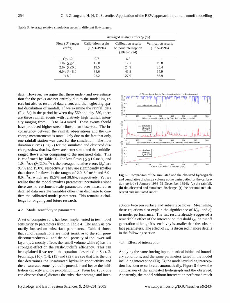
Figure 6 shows the comparison of the simulated andobserved hydrographs (Fig. 6b), and the accumulated dis-charges for the simulated and observed data at the outlet ofthe Geer river basin (Fig. 6c). Clearly, the pattern of the wa-tershed response to the atmospheric forcing is well captured.The base flow is quite accurately reproduced in the calibra-tion period except for the beginning 3 months, mostly dueto the model warming up effect. Most peaks are simulatedwith reasonable accuracy although some peaks in the periodfrom 340 days to 480 days (Fig. 6b) are underestimated. Wealso observed that three peaks in the period from 560 daysto 580 days are overestimated compared with the measured



Table 3. Average relative simulation errors in different flow ranges.

Averaged relative errorsδp (%)

Flow (Q) ranges Calibration results Calibration results Verification results(m3/s) (1993–1994) without interception (1995–1996)

(1993–1994)

Q≤1.0 9.7 6.5 –1.0<Q≤2.0 15.0 17.7 19.82.0<Q≤6.0 19.5 24.9 25.46.0<Q≤8.0 38.6 41.9 15.9

>8.0 22.2 27.0 36.9

data. However, we argue that these under- and overestima-tion for the peaks are not entirely due to the modelling er-rors but also as result of data errors and the neglecting spa-tial distribution of rainfall. If we examine the rainfall data(Fig. 6a) in the period between day 560 and day 580, thereare three rainfall events with relatively high rainfall inten-sity ranging from 11.8 to 24.4 mm/d. These events shouldhave produced higher stream flows than observed. The in-consistency between the rainfall observations and the dis-charge measurements is most likely due to the fact that onlyone rainfall station was used for the simulation. The flowduration curves (Fig. 7) for the simulated and observed dis-charges show that low flows are better simulated than middle-ranged flows when comparing to the measured data. Thisis confirmed by Table 3. For low flows (Q≤1.0 m3/s, and1.0 m3/s<Q≤2.0 m3/s), the averaged relative errors (δp) are9.7% and 15.0%, respectively. They are significantly smallerthan those for flows in the ranges of 2.0–6.0 m3/s and 6.0–8.0 m3/s, which are 19.5% and 38.6%, respectively. Yet werealise that the model involves parameter uncertainties sincethere are no catchment-scale parameters ever measured ordetailed data on state variables other than discharge to con-firm the calibrated model parameters. This remains a chal-lenge for ongoing and future research.

4.2 Model sensitivity to parameters

A set of computer runs has been implemented to test modelsensitivity to parameters listed in Table 4. The analysis pri-marily focused on subsurface parameters. Table 4 showsthat runoff simulations are most sensitive to the soil pore-disconnectednessλ and the soil porosity of the lower soillayerε′s . λ mostly affects the runoff volume whileε′s has thestrongest effect on the Nash-Sutcliffe efficiency. This canbe explained if we recall the equations described in Sect. 2.From Eqs. (10), (14), (15) and (32), we see thatλ is the onethat determines the unsaturated hydraulic conductivity andthe unsaturated zone hydraulic potential, and hence the infil-tration capacity and the percolation flux. From Eq. (33), onecan observe thatε′s dictates the subsurface storage and inter-

0 100 200 300 400 500 600 700

0

10

20

30

40

50

a) Observed rainfall at the Bierset gauging station − calibration period

rain

fall

inte

nsity

(m

m/d

)

daily rainfall intensity

0 100 200 300 400 500 600 7000

5

10b) Discharges at the outlet of the Geer river − calibration period

Dis

char

ge −

(m3 /s

)

simulatedobservedR2

NS=0.71

0 100 200 300 400 500 600 7000

2

4

6

8

10

12x 10

7 c) Cumulative discharges at the outlet of the Geer river − calibration period

time (01/01/1993 −31/12/1994) − (days)

Cum

ulat

ive

disc

harg

e −

(m3 )

simulatedobservedδ

B=0.76%

Fig. 6. Comparison of the simulated and the observed hydrographand cumulative discharge volume at the basin outlet for the calibra-tion period (1 January 1993–31 December 1994):(a) the rainfall,(b) the observed and simulated discharge,(c) the accumulated ob-served and simulated runoff.

actions between surface and subsurface flows. Meanwhile,these equations also explain the significance ofKss andε′uin model performance. The test results already suggested aremarkable effect of the interception thresholdidc on runoffgeneration although it’s sensitivity is smaller than the subsur-face parameters. The effect ofidc is discussed in more detailsin the following section.

4.3 Effect of interception

Applying the same forcing input, identical initial and bound-ary conditions, and the same parameters tuned in the modelincluding interception (Fig. 6), the model excluding intercep-tion has been re-calibrated automatically. Figure 8 shows thecomparison of the simulated hydrograph and the observed.Apparently, the model without interception performed much



Stream flow duration curve_calibration

0

2

4

6

8

10

0 20 40 60 80 100

percentage of discharge exceedance

dis

charg

e (

m³/

s)

simulated observed

Fig. 7. Flow duration curves for the model calibration results andthe observed data.

Table 4. Sensitivity of the model output to parameters.

Parameters δV (%) δNS (%)

λ (–) 190 1177ε′s (–) 109 1729

Kss (m/d) 81 45ε′u (–) 77 89

Ksu (m/d) 10 6idc (mm/d) 10 5

worse than the one with interception:R2NS is 14% lower, and

δB is 187% larger. Figure 9 shows the flow duration curvesfor the simulation outputs of both the models with and with-out interception, as well as for the observed flow records. To-gether with analysing the averaged relative errorδp presentedin Table 3, we can find that the model without interceptiondoes not cover the full range of the low flows, suggestingerroneous simulation of the water balance. This is becausemore water, which would have been intercepted, is adding tothe subsurface stores, participating in the surface and subsur-face flux exchanges, and subsequently contributes to streamflow. Especially during the smaller rainfall events, the partof the rainfall flux that would have been intercepted leads toa higher antecedent soil moisture state, which either initiatesa quicker surface runoff or gives rise to higher stream flowduring the low flow regime. In the simulation without inter-ception, we see that low flows are higher than observed, e.g.in the period of the last 120 days (Fig. 8a). However, as themodel tries to maintain overall performance in terms of to-tal volume, the simulated flow mass curve enters into a moreor less constant slope, which does not follow the bending ofthe observed flow mass curve after 360 days (Fig. 8b). In

0 100 200 300 400 500 600 7000

2

4

6

8

10a) Discharges at the outlet of the Geer river

time (01/01/1993 − 31/12/1994) − (days)

Dis

char

ge −

(m3 /s

)

simulated− without interceptionobservedR2

NS=0.61

0 100 200 300 400 500 600 7000

2

4

6

8

10

12x 10

7 b) Cumulative discharges at the outlet of the Geer river

time (01/01/1993 − 31/12/1994) − (days)

Cum

ulat

ive

disc

harg

e −

(m3 )

simulated − without interceptionobservedδ

B=2.2%

Fig. 8. Simulated discharge using the model without interceptionafter optimisation (1 January 1993–31 December 1994):(a) ob-served and simulated discharge,(b) accumulated observed and sim-ulated runoff.

Stream flow duration curve

0

2

4

6

8

10

0 20 40 60 80 100


dis

charg

e (

m³/

s)

sim_with interception

observed

sim_without interception

Fig. 9. Flow duration curves for the model calibration results (withinterception and without interception) and the observed data.

Fig. 10, one can notice that without interception, the soil sat-uration is steadily increasing over time (dotted lines) for eachof the REWs presented. However, one would expect that fora multiple-year simulation, the soil moisture state would pre-serve an equilibrium state while varying seasonally.

4.4 Model verification

The approach suggested by Klemes (1986) has been adoptedto verify the model. A reversed calibration/verification testwas also carried out. From Fig. 11, we can see that the modelis able to reproduce most peaks except the one on day 525.



0 0.5 1 1.5 20.5

0.6

0.7

0.8

0.9

1a) REW 1

t − (year)

s (−

)

without interceptionwith interception

0 0.5 1 1.5 20.5

0.6

0.7

0.8

0.9

1b) REW 53

t − (year)

s (−

)


0 0.5 1 1.5 20.5

0.6

0.7

0.8

0.9

1c) REW 54

t − (year)

s (−

)


0 0.5 1 1.5 20.5

0.6

0.7

0.8

0.9

1d) REW 61

t − (year)

s (−

)


Fig. 10.Comparison of the hill-slope soil moisture dynamics simu-lated with and without interception process in the model. REW 53,REW54 and REW 61 compose a hill-slope of the catchment in thesouthern side of the Geer river.

Table 5. Model performance in the split-sample test runs.

test δB (%) R2NS

calibration (1993–1994) 0.76 0.71verification (1995–1996) 4.79 0.61reversed calibration (1995–1996) 4.14 0.65reversed verification (1993–1994) 3.82 0.68

The observed discharge on this day is 9 m3/s and the rainfallcausing this peak is 28 mm/d. Scanning all rainfall eventsand peak responses in the catchment in the period of 1993–1996, this data point is an exception lying outside the gen-eral rainfall runoff relation of the catchment. It is likely dueto either a measurement error or the inadequate density ofthe rainfall observation network. As a result, it is not usedfor model performance analysis. In this verification run, lowflows in most of the time are underestimated, which can beconfirmed from the flow duration curve (Fig. 12). Actually,from Fig. 11b, we can find that the observed flow data exhibitmore or less constant base flows and show no remarkable de-pleting trend in the dry period over the time from 1995 to1996. This appearance is also shown in Fig. 12 in whichthere is an abrupt change of the probability distribution forthe observed discharges from 2.0 m3/s to 1.0 m3/s.

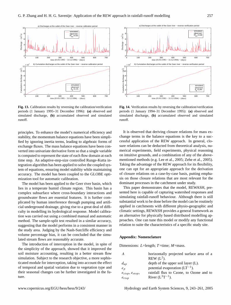
Table 5 reports the summary of the model performance ineach of the calibration/verification runs. Figures 13 and 14present the reversed calibration/verification tests. All theseresults demonstrate that the model, giving a similar volumeerror and Nash-Sutcliffe efficiency in each of the simulations,performs in a very consistent manner.

0 100 200 300 400 500 600 700

0

10

20

30

40

50

a) Observed rainfall at the Bierset gauging station − verification period

rain

fall

inte

nsity

(m

m/d

)

daily rainfall intensity

0 100 200 300 400 500 600 7000

5

10b) Discharges at the outlet of the Geer river − verification period

Dis

char

ge −

(m3 /s

)

simulatedobservedR2

NS=0.61

0 100 200 300 400 500 600 7000

2

4

6

8

10

12x 10

7 c) Cumulative discharges at the outlet of the Geer river − verification period

time (01/01/1995 −31/12/1996) − (days)

Cum

ulat

ive

disc

harg

e −

(m3 )

simulatedobservedδ

B=4.8%

Fig. 11. Model verification results:(a) observed daily rainfall in-tensity at the Bierset station;(b) comparison of the simulated andobserved daily discharge at the outlet of the Geer river basin;(c)comparison of the simulated and observed runoff volume (1 Jan-uary 1995–31 December 1996).

Stream flow duration curve_verification

0

2

4

6

8

10

12

0 20 40 60 80 100


dis

charg

e (

m³/

s) simulated observed

Fig. 12. Flow duration curves for the model verification results andthe observed data.

5 Summary and conclusions

This paper has presented a comprehensive and convincingapplication of the REW-based spatially-distributed model toan actual meso-scale basin, with considerable spatial hetero-geneity and between-REW interactions. The model has beenimproved by the addition of the interception process, im-proved transpiration scheme and improved saturation-excessflow area formulation. At the watershed-scale, surfaceand subsurface interaction, climate feedback, hill-slope andchannel network have been fully coupled, based on physical



0 100 200 300 400 500 600 7000

2

4

6

8

10a) Discharges at the outlet of the Geer river − reverse calibration period

time (01/01/1995 − 31/12/1996) − (days)

Dis

char

ge −

(m3 /s

)

simulatedobservedR2

NS=0.65

0 100 200 300 400 500 600 7000

2

4

6

8

10

12x 10

7 b) Cumulative discharges at the outlet of the Geer river − reverse calibration period

time (01/01/1995 − 31/12/1996) − (days)

Cum

ulat

ive

disc

harg

e −

(m3 )

simulatedobservedδ

B=4.1%

Fig. 13. Calibration results by reversing the calibration/verificationperiods (1 January 1995–31 December 1996):(a) observed andsimulated discharge,(b) accumulated observed and simulatedrunoff.

principles. To enhance the model’s numerical efficiency andstability, the momentum balance equations have been simpli-fied by ignoring inertia terms, leading to algebraic forms ofexchange fluxes. The mass balance equations have been con-verted into univariate derivative form so that a single variableis computed to represent the state of each flow domain at eachtime step. An adaptive-step-size controlled Runge-Kutta in-tegration algorithm has been applied to solve the coupled sys-tem of equations, ensuring model stability while maintainingaccuracy. The model has been coupled to the GLOBE opti-mization tool for automatic calibration.

The model has been applied to the Geer river basin, whichlies in a temperate humid climate region. This basin has acomplex subsurface where cross-boundary interactions andgroundwater flows are essential features. It is further com-plicated by human interference through pumping and artifi-cial underground drainage, giving rise to a great deal of diffi-culty in modelling its hydrological response. Model calibra-tion was carried out using a combined manual and automaticmethod. The sample-split test resulted in a similar accuracy,suggesting that the model performs in a consistent manner inthe study area. Judging by the Nash-Sutcliffe efficiency andvolume percentage bias, it can be concluded that the simu-lated stream flows are reasonably accurate.

The introduction of interception in the model, in spite ofthe simplicity of the approach, showed that it improved thesoil moisture accounting, resulting in a better stream flowsimulation. Subject to the research objective, a more sophis-ticated module for interception, taking into account the effectof temporal and spatial variation due to vegetation type andtheir seasonal changes can be further investigated in the fu-ture.

0 100 200 300 400 500 600 7000

2

4

6

8

10a) Discharges at the outlet of the Geer river − reverse verification period

time (01/01/1993 − 31/12/1994) − (days)

Dis

char

ge −

(m3 /s

)

simulatedobservedR2

NS=0.68

0 100 200 300 400 500 600 7000

2

4

6

8

10

12x 10

7 b) Cumulative discharges at the outlet of the Geer river − reverse verification period

time (01/01/1993 − 31/12/1994) − (days)

Cum

ulat

ive

disc

harg

e −

(m3 )

simulatedobservedδ

B=3.8%

Fig. 14.Verification results by reversing the calibration/verificationperiods (1 January 1994–31 December 1995):(a) observed andsimulated discharge,(b) accumulated observed and simulatedrunoff.

It is observed that deriving closure relations for mass ex-change terms in the balance equations is the key to a suc-cessful application of the REW approach. In general, clo-sure relations can be deducted from theoretical analysis, nu-merical experiments, field experiments, physical reasoningon intuitive grounds, and a combination of any of the above-mentioned methods (e.g. Lee et al., 2005; Zehe et al., 2005).Taking the advantage of the REW approach for its flexibility,one can opt for an appropriate approach for the derivationof closure relations on a case-by-case basis, putting empha-sis on those closure relations that are most relevant for thedominant processes in the catchment under study.

This paper demonstrates that the model, REWASH, pre-sented here is capable of capturing watershed responses andsimulating rainfall-runoff behaviour. Although there is stillsubstantial work to be done before the model can be routinelyapplied in catchments with different physio-geographic andclimatic settings, REWASH provides a general framework asan alternative for physically based distributed modelling ap-proaches. One can tune this model or modify any functionalrelation to suite the characteristics of a specific study site.

Appendix: Nomenclature

Dimensions:L=length;T =time;M=mass.

A horizontally projected surface area of aREW (L2).

dup depth of the upper soil layer (L).ep potential evaporation (LT−1).ectop, eotop,ertop

rainfall flux to Czone, to Ozone and toRiver (L3T−1).



eca , ecu, eco interception flux from Czone, infiltrationflux to Uzone, flux between Czone andOzone (L3T−1).

eoa , eos , eor ,eoc

evaporation flux from Ozone, flux be-tween Ozone and Szone, flux betweenOzone and River, flux between Ozoneand Czone (L3T−1).

eua , euc, eus transpiration fux in Uzone, infiltrationflux from Czone, percolation flux toSzone (L3T−1).

esu, eso the counterpart ofeus andeso.esr , esi , esa flux between Szone and River, flux ex-

change between the neighbouring REWs,groundwater abstraction (L3T−1).

era , erin, erout evaporation from River, flux from up-stream River, flux to the downstreamRiver (L3T−1).

ers , ero the counterpart ofesr andeor .f infiltration capacity (L3T−1).g gravitational acceleration (LT−2).G groundwater abstraction or recharge rate

(L3T−1).hc capillary pressure head (L).ho, hr , hs total hydraulic head for Ozone, River and

Szone (L).i precipitation intensity (LT−1).idc interception threshold for Czone (LT−1).Ksu,Ku saturated and effective hydraulic conduc-

tivity for Uzone (LT−1).Ksr ,Kss saturated hydraulic conductivity for

riverbed and Szone (LT−1).lr length of the river channel (L).m average cross-sectional area (L2).n Manning roughness coefficient (TL1/3).Pr wetted perimeter of the river cross section

(L).Qsi ,Qoi , Qo simulated discharge, observed discharge

at the time step i,mean of the observeddischarge (L3T−1).

Qi+,Qi−,Qim

discharges after the parameter perturba-tion by ±50% at time stepi, dischargeafter the accepted manual calibration attime stepi (L3T−1).

R2NS Nash-Sutcliffe efficiency (–).R2NS+

, R2NS−

,R2NSm, R2

NS

values after parameter perturbation by±50%, and after the accepted manual cal-ibration (–).

s sink or source term.Sc, So, Su, Ss ,Sr

storage of Czone, Ozone, Uzone, Szoneand River (M).

vo, vr velocity of the flow in the River andOzone (LT−1).

wr width of the river channel (L).yo depth of flow sheet over the overland flow

zone surface (L).

yr water depth of the river channel (L).ys , yu average depth of Szone and Uzone (L).zr , zs , zsurf average elevation for river bed, ground

surface and soil bottom (L).Z average soil depth (L).αsf scaling factor for Ozone area computa-

tion (–).αsi lumped scaling factor for regional

groundwater flow (L2T−1).αus scaling factor for flux exchange between

Uzone and Szone (–).δB discharge volume percentage bias (–).δNS relative change in Nash-Sutcliffe effi-

ciency (–).δV relative change in percentage bias (–).δp average relative error (–).ε′u, ε

′s porosity of the upper and lower soil layer

(–).εu, εs effective soil porosity of Uzone and

Szone (–).φ generic thermodynamic property.γo average surface slope angle of Ozone in

radian.γr average slope angle of the channel bed in

radian.λ soil pore-disconnectedness index (–).3r depth of the transition zone of the river

bed for the base flow (L).3s typical length scale for the exfiltration

flux (seepage) (L).3u length scale of the wetting front for infil-

tration (L).µ soil pore size distribution index (–).θf field capacity of Uzone (–).ρ water density (ML−3).ωo, ωc, ωo area fraction of the saturation-excess

overland flow domain, infiltration-excessflow domain and the unsaturated flow do-main (–).

ξ Darcy-Weisbach friction factor for thechannel routing (–).

ψb air entry pressure head at Uzone (L).

Acknowledgements.This research has been funded by the DelftCluster project Oppervlaktewater hydrologie: 06.03.04. We arevery grateful to D. P. Solomatine of UNESCO-IHE for providingthe GLOBE optimisation software for automatic calibration.We acknowledge that the data applied in this research wereacquired through the project DAUFIN, sponsored by the EuropeanCommission within FP5: EVK1-CT1999-00022. S. Brouyere andA. Dassargues of the University of Liege (Belgium) provided thebasic data about the geological and hydrogeological conditions ofthe Geer basin. The Royal Meteorological Observatory (KMI) inBrussels and E. Roulin provided the digital elevation maps andthe hydro-meteorological data. The valuable comments provided



by E. Zehe, an anonymous referee and the editor, M. Sivapalanhave considerably improved the manuscript. It is highly ap-preciated that P. Reggiani provided the original computer code,based on which the numerical model REWASH has been developed.

Edited by: M. Sivapalan

References

Abbott, M. B., Bathurst, J. C., Cunge, J. A., O’Connell, P. E., andRasmussen, J.: An introduction to the European Hydrologic Sys-tem Systeme Hydrologique Europeen, SHE, 1: History and phi-losophy of a physically based, distributed modelling system, J.Hydrol., 87, 45–59, 1986a.

Abbott, M. B., Bathurst, J. C., Cunge, J. A., O’Connell, P. E., andRasmussen, J.: An introduction to the European Hydrologic Sys-tem Systeme Hydrologique Europeen, SHE, 2: Structure of aphysically based, distributed modelling system, J. Hydrol., 87,61–77, 1986b.

Bastidas, L.A., Gupta, H. V., Sorooshian, S., Shuttleworth, W. J.,and Yang, Z. L.: Sensitivity analysis of land surface scheme us-ing multicriteria methods, J. Geophys. Res., 104, 19 481–19 490,1999.

Bergstrom, S. and Forsman, A.: Development of a conceptual de-terministic rainfall-runoff model, Nordic Hydrol., 4, 147–170,1973.

Bergstrom, S.: The HBV model, in: Computer models of watershedhydrology, edited by: Singh, V. P., Water Resources Publications,USA, 443–520, 1995.

Beven, K. J.: Infiltration into a class of vertically non-uniform soils,Hydrol. Sci. J., 29, 425–434, 1984.

Beven, K. J.: Changing ideas in hydrology: the case of physicallybased models, J. Hydrol., 105, 157–172, 1989.

Beven, K. J.: Prophesy, reality and uncertainty in distributed hydro-logical modelling, Adv. Water Res., 16, 41–51, 1993.

Beven, K. J.: A discussion of distributed hydrological modelling,in: Distributed hydrological modelling, edited by: Abbott, M. B.and Refsgaard, J. C., Kluwer Academic Publishers, Dordrecht,The Netherlands, 255–278, 1996a.

Beven, K. J.: Response to comments on “A discussion of distributedhydrological modelling” by Refsgaard, J. C. et al., in: Distributedhydrological modelling, edited by: Abbott, M. B. and Refsgaard,J. C., Kluwer Academic Publishers, Dordrecht, The Netherlands,289–295, 1996b.

Beven, K. J.: Equifinality and uncertainty in geomorphologicalmodelling, in: The scientific nature of geomorphology, editedby: Rhoads, B. L. and Thorn, C. E., John Wily & Sons, Chich-ester, UK, 289–313, 1996c.

Beven, K. J.: Towards an alternative blueprint for a physically baseddigitally simulated hydrologic response modelling system, Hy-drol. Process., 16, 189–206, 2002.

Beven, K. and Binly, A.: The future of distributed models: modelcalibration and uncertainty predication, Hydrol. Process., 6, 279–298, 1992.

Beven, K. J., Calver, A., and Morris, E.: The Institute of Hydrologydistributed model, Institute of Hydrology Report No. 98, UK,1987.

Beven, K. J., Lamb, R., Quinn, P., Romanowicz, R., and Freer,J.: TOPMODEL, in: Computer models of watershed hydrol-

ogy, edited by: Singh, V. P., Water Resources Publications, USA,627–668, 1995.

Bloschl, G. and Sivapalan, M.: Scale issues in hydrological mod-elling – a review, Hydrol. Process., 9, 251–290, 1995.

Boyle, D. P., Gupta, H. V., and Sorooshian, S.: Toward improvedcalibration of hydrologic models: Combining the strengths ofmanual and automatic methods, Water Resour. Res., 36, 3663–3674, 2000.

Brooks, R. H. and Corey, A. T.: Hydraulic properties of porousmedia, Hydrol. Pap. No. 3, Colorado State Univ., Fort Collins,1964.

Brun, R., Reichert, P., and Kunsch H. R.: Practical identifiabilityanalysis of large environmental simulation models, Water Re-sour. Res., 37, 1015–1030, 2001.

Burnash, R. J. C., Ferral, R. L., and McGuire, R. A.: A Generalizedstreamflow simulation system – Conceptual modeling for digi-tal computers, US Department of Commerce, National WeatherService and State of Califonia, Department of Water Resources,1973.

Burnash, R. J. C.: The NWS river forecast system – Catchmentmodelling, in: Computer models of watershed hydrology, editedby: Singh, V. P., Water Resources Publications, USA, 311–366,1995.

Calver, A and Wood, W. L.: The Institute of Hydrology distributedmodel, in: Computer models of watershed hydrology, editedby: Singh, V. P., Water Resources Publications, USA, 595–626,1995.

Cash, J. R. and Karp, A. H.: ACM Transactions on MathematicalSoftware, 16, 201–222, 1990.

Doorenbos, J. and Kassam A. H.: Yield response to water, FAOirrigation and drainage paper 33, Food and Agriculture Organi-sation, Rome, 1979.

Dunne, T. and Black, R. D.: Partial area contributions to stormrunoff in a small New England watershed, Water Resour. Res.,6, 1296–1311, 1970.

Dunne, T.: Field studies of hillslope flow processes, in: HillslopeHydrology, edited by: Kirkby, M. J., John Wily & Sons, Chich-ester, UK, 227–293, 1978.

Freer, J., Beven, K., and Ambroise, B.: Bayesian estimation of un-certainty in runoff prediction and the value of data: An applica-tion of the GLUE approach, Water Resour. Res., 32, 2161–2173,1996.

Freeze, R. A. and Harlan, R. L.: Blueprint for a physically-based,digitally-simulated hydrologic response model, J. Hydrol., 9,237–258, 1969.

Grayson, R. B., Moore, I. D., and McMahon, T. A.: Physicallybased hydrologic modeling, 1, A terrain-based model for inves-tigative purposes, Water Resour. Res., 28, 2639–2658, 1992a.

Grayson, R. B., Moore, I. D., and McMahon, T. A.: Physicallybased hydrologic modeling, 2, Is the concept realistic?, WaterResour. Res., 28, 2659–2666, 1992b.

Hewlett, J. D. and Hibbert, A. R.: Factors affecting the response ofsmall watersheds to precipitation in humid areas, in: Proceedingsof 1st International Symposium on Forest Hydrology, edited by:Sopper, W. E. and Lull, H. W., Pergamon, 275–290, 1967.

Hornberger, G. M. and Spear, R. C.: An approach to the preliminaryanalysis of environmental systems, J. Environ. Mgmt., 12, 7–18,1981.



Kirkby, M. J.: TOPMODEL: A personal view, Hydol. Process., 11,1087–1097, 1997.

Klemes, V.: Operational testing of hydrological simulation models,Hydrol. Sci. J., 31, 13–24, 1986.

Lee, H., Sivapalan, M., and Zehe E.: Representative Elemen-tary Watershed (REW) approach, a new blueprint for distributedhydrologic modelling at the catchment scale: development ofclosure relations, in: Predicting ungauged streamflow in themackenzie river basin: today’s techniques and tomorrow’s so-lutions, edited by: Spence, C., Pomeroy, J. W., and Pietroniro,A., Canadian Water Resources Association (CWRA), Ottawa,Canada, 165–218, 2005.

Lindstrom, G., Johansson, B., Persson, M., Gardelin, M., andBergstrom, S.: Development and test of the distributed HBV-96hydrological model, J. Hydrol., 201, 272–288, 1997.

Nash, J. E. and Sutcliffe, J. V.: River flow forecasting through con-ceptual models, Part I: a discussion of principles, J. Hydrol., 10,282–290, 1970.

Newham, L. T. H., Norton, J. P., Prosser, I. P., Croke, B. F. W., andJakeman A. J.: Sensitivity analysis for assessing the behaviourof a landscape-based sediment and transport model, Environ.Model. & Soft., 18, 741–751, 2003.

O’Connell, P. E. and Todini E.: Modelling of rainfall, flow and masstransport in hydrological systems: an overview, J. Hydrol., 175,3–16, 1996.

Press, W. H., Teukolsky, S. A., Vetterling, W. T., and Flannery B.P.: Numerical recipes in C: The art of scientific computing, 2ndEdition, Cambridge University Press, 710–722, 1992.

Refsgaard, J. C. and Storm, B.: MIKE SHE, in: Computer modelsof watershed hydrology, edited by: Singh, V. P., Water ResourcesPublications, USA, 809–846, 1995.

Refsgaard, J. C., Storm, B., and Abbott, M. B.: Comment on “Adiscussion of distributed hydrological modelling” by K. Beven,in: Distributed hydrological modelling, edited by: Abbott, M. B.and Refsgaard, J. C., Kluwer Academic Publishers, Dordrecht,The Netherlands, 279–287, 1996.

Reggiani, P. and Schellekens, J.: Modelling of hydrological re-sponses: the representative elementary watershed approach as analternative blueprint for watershed modelling, Hydrol. Process.,17, 3785–3789, 2003.

Reggiani, P., Sivapalan M., and Hassanizadeh, S. M.: A unifyingframework of watershed thermodynamics: balance equations formass, momentum, energy and entropy and the second law of ther-modynamics, Adv. Water Res., 22, 367–368, 1998.

Reggiani, P., Sivapalan, M., and Hassanizadeh, S. M.: Conservationequations governing hillslope responses: Physical basis of waterbalance, Water Resour. Res., 38, 1845–1863, 2000.

Reggiani, P., Hassanizadeh, S. M., Sivapalan, M., and Gray, W. G.:A unifying framework of watershed thermodynamics: Constitu-tive relationships, Adv. Water Res., 23, 15–39, 1999.

Reggiani, P., Sivapalan, M., Hassanizadeh, S. M., and Gray, W. G.:Coupled equations for mass and momentum balance in a streamnetwork: theoretical derivation and computational experiments,Proc. R. Soc. Lond. A(2001), 457, 157–189, 2001.

Reggiani, P. and Rientjes, T. H. M.: Flux parameterization in theRepresentative Elementary Watershed (REW) Approach: appli-cation to a natural basin: Water Resour. Res., 41, W04013,doi:10.1029/2004WR003693, 2005.

Rijtema, P. E. and Aboukhaled A.: Crop water use, in: Research oncrop and water use, salt affected soils and drainage in the ArabRepublic of Egypt, edited by: Aboukhaled, A., Arar, A., Balba,A. M. et al., FAO, Near East Regional Office, Cairo, 5–61, 1975.

Saltelli, A.: What is sensitivity analysis?, in: Sensitivity analysis,edited by: Saltelli, A., Chan, K., and Scott, E. M., John Wiley &Sons, Ltd., Chichester, UK, 3–12, 2000.

Savenije, H. H. G.: Equifiniality, a blessing in disguise?, Hydrol.Process., 15, 2835–2838, 2001.

Savenije, H. H. G.: The importance of interception and why weshould delete the term evapotranspiration from our vocabulary,Hydrol. Process., 18, 1507–1511, 2004.

Savenije, H. H. G.: Interception, The Encyclopaedia of Water, Wi-ley, 2005.

Senarath, S. U. S., Ogden, F. L., Downer, C. W., and Sharif, H.O.: On the calibration and verification of two-dimensional, dis-tributed, Hortonian, continuous watershed models, Water Re-sour. Res., 36, 1495–1510, 2000.

Sivapalan, M., Viney, N. R., and Jeevaraj, C. G.: Water and saltbalance modelling to predict the effects of land use changes inforested catchments: 3. The large catchment model, Hydrolog.Process., 10, 429–4446, 1996.

Solomatine, D. P.: Genetic and other global optimization algorithms– comparison and use in calibration problems, in: Proceedings ofthe 3rd International Conference on Hydroinformatics, Copen-hagen, Denmark, Balkema Publishers, 1021–1028, 1998.

Solomatine, D. P.: The use of global random search methods formodels calibration, in: Proceedings of XXVIth Congress of theInternational Association for Hydraulic Research (IAHR), vol. 1,London, 224–229, 1995.

Sorooshian, S., Duan, Q., and Gupta, V. K.: Calibration of rainfall-runoff models: Application of global optimization to the Sacra-mento Soil Moisture Accounting Model, Water Resour. Res., 29,1185–1194, 1993.

Strahler, A. N.: Quantitative analysis of watershed geomorphology,American Geophysical Union Transactions, 38, 913–920, 1957.

Tarboton, D. G.: A new method for the determination of flow di-rections and contributing areas in grid digital elevation models,Water Resour. Res., 33, 309–319, 1997.

Todini, E.: The ARNO rainfall-runoff model, J. Hydrol., 175, 339–382, 1996.

Troch, P. A., De Troch, F. P., and Brutsaert, W.: Water table depthto describe initial conditions prior to storm rainfall in humid re-gions, Water Reour. Res., 29, 427–434, 1993.

Wagener, T.: Evaluation of catchment models, Hydrol. Process., 17,3375–3378, 2003.

Wagener, T., Wheater, H. S., and Gupta, H. V.: Rainfall runoffmodelling in gauged and ungauged catchment, Imperial CollegePress, London, UK, 2004.

Zehe, E., Lee, H., and Sivapalan, M.: Derivation of closure relationsand commensurate state variables for mesoscale hydrologicalmodels using dynamical upscaling, in: Predictions in ungaugedbasins: international perspectives on state-of-the-art and path-ways forward, edited by: Franks, S. W., Sivapalan, M., Takeuchi,K., and Tachikawa, Y., IAHS Press, Wallingford, Oxon, UK, inpress, 2005.

Zhang, G., Reggiani, P., Rientjes, T. H. M., and Hassanizadeh,S. M.: Modeling rainfall-runoff relation by the Representa-tive Elementary Watershed Approach, in: Proceedings of NCR-



days 2002: Current themes in Dutch river research, edited by:Leuven, R. S. E. W., van Os, A. G., and Nienhuis, P. H.,NCR-publication 20-2003, Netherlands Centre for River Stud-ies, Delft, The Netherlands, 20–22, 2003.

Zhang, G. P., Fenicia, F., Rientjes, T. H. M., Reggiani, P., andSavenije, H. H. G.: Effects of subsurface parameterisation onrunoff generation in the Geer basin, in: Proceedings of NCR-days 2003: Dealing with Floods within Constraints, edited by:Douben, N. and van Os, A. G., NCR publication 24-2004,Netherlands Centre for River Studies, Delft, The Netherlands,68–70, 2004a.

Zhang, G. P., Fenicia, F., Rientjes, T. H. M., Reggiani, P., andSavenije, H. H. G.: Application and development of a catchment-scale rainfall-runoff model using the REW approach, Geophys.Res. Abstr., 6, EGU04-A-01583, European Geosciences Union,SRef-ID: 1607-7962/gra/EGU04-A-01583, 2004b.

Zhang, G. P., Fenicia, F., Rientjes, T. H. M., Reggiani, P. andSavenije, H. H. G.: Modeling runoff generation in the Geer RiverBasin with improved model parameterizations to the REW ap-proach, Phys. Chem. Earth, 30, 285–296, 2005a.

Zhang, G. P., Savenije, H. H. G., Fenicia, F., Rientjes, T. H. M., andReggiani, P.: Implications of hydrological modelling and obser-vations in the Alzette river basin, in: Proceedings of NCR-days2004: Research for managing rivers; present and future issues, inpress, 2005b.


http://direct.sref.org/1607-7962/gra/EGU04-A-01583

sciences earth system hydrology and rainfall-runoff ... · pdf filehydrology and earth system...

Documents