scientiﬁc computing: an introductory survey value problems numerical methods for bvps boundary...

Boundary Value ProblemsNumerical Methods for BVPs

Scientific Computing: An Introductory SurveyChapter 10 – Boundary Value Problems for

Ordinary Differential Equations

Prof. Michael T. Heath

Department of Computer ScienceUniversity of Illinois at Urbana-Champaign

Copyright c© 2002. Reproduction permittedfor noncommercial, educational use only.

Michael T. Heath Scientific Computing 1 / 45


Outline

1 Boundary Value Problems

2 Numerical Methods for BVPs



Boundary ValuesExistence and UniquenessConditioning and Stability

Boundary Value Problems

Side conditions prescribing solution or derivative values atspecified points are required to make solution of ODEunique

For initial value problem, all side conditions are specified atsingle point, say t0

For boundary value problem (BVP), side conditions arespecified at more than one point

kth order ODE, or equivalent first-order system, requires kside conditions

For ODEs, side conditions are typically specified atendpoints of interval [a, b], so we have two-point boundaryvalue problem with boundary conditions (BC) at a and b.




Boundary Value Problems, continuedGeneral first-order two-point BVP has form

y′ = f(t, y), a < t < b

with BCg(y(a),y(b)) = 0

where f : Rn+1 → Rn and g : R2n → Rn

Boundary conditions are separated if any given componentof g involves solution values only at a or at b, but not both

Boundary conditions are linear if they are of form

Ba y(a) + Bb y(b) = c

where Ba,Bb ∈ Rn×n and c ∈ Rn

BVP is linear if ODE and BC are both linearMichael T. Heath Scientific Computing 4 / 45



Example: Separated Linear Boundary Conditions

Two-point BVP for second-order scalar ODE

u′′ = f(t, u, u′), a < t < b

with BCu(a) = α, u(b) = β

is equivalent to first-order system of ODEs[y′1y′2

]=

[y2

f(t, y1, y2)

], a < t < b

with separated linear BC[1 00 0

] [y1(a)y2(a)

]+

[0 01 0

] [y1(b)y2(b)

]=

[αβ

]Michael T. Heath Scientific Computing 5 / 45



Existence and Uniqueness

Unlike IVP, with BVP we cannot begin at initial point andcontinue solution step by step to nearby points

Instead, solution is determined everywhere simultaneously,so existence and/or uniqueness may not hold

For example,u′′ = −u, 0 < t < b

with BCu(0) = 0, u(b) = β

with b integer multiple of π, has infinitely many solutions ifβ = 0, but no solution if β 6= 0




Existence and Uniqueness, continued

In general, solvability of BVP

y′ = f(t, y), a < t < b

with BCg(y(a),y(b)) = 0

depends on solvability of algebraic equation

g(x,y(b;x)) = 0

where y(t;x) denotes solution to ODE with initial conditiony(a) = x for x ∈ Rn

Solvability of latter system is difficult to establish if g isnonlinear



Shooting MethodFinite Difference MethodCollocation MethodGalerkin Method

Numerical Methods for BVPs

For IVP, initial data supply all information necessary tobegin numerical solution method at initial point and stepforward from there

For BVP, we have insufficient information to beginstep-by-step numerical method, so numerical methods forsolving BVPs are more complicated than those for solvingIVPs

We will consider four types of numerical methods fortwo-point BVPs

Shooting

Finite difference

Collocation

Galerkin




Shooting MethodIn statement of two-point BVP, we are given value of u(a)

If we also knew value of u′(a), then we would have IVP thatwe could solve by methods discussed previously

Lacking that information, we try sequence of increasinglyaccurate guesses until we find value for u′(a) such thatwhen we solve resulting IVP, approximate solution value att = b matches desired boundary value, u(b) = β




Shooting Method, continued

For given γ, value at b of solution u(b) to IVP

u′′ = f(t, u, u′)

with initial conditions

u(a) = α, u′(a) = γ

can be considered as function of γ, say g(γ)

Then BVP becomes problem of solving equation g(γ) = β

One-dimensional zero finder can be used to solve thisscalar equation




Example: Shooting MethodConsider two-point BVP for second-order ODE

u′′ = 6t, 0 < t < 1

with BCu(0) = 0, u(1) = 1

For each guess for u′(0), we will integrate resulting IVPusing classical fourth-order Runge-Kutta method todetermine how close we come to hitting desired solutionvalue at t = 1

For simplicity of illustration, we will use step size h = 0.5 tointegrate IVP from t = 0 to t = 1 in only two steps

First, we transform second-order ODE into system of twofirst-order ODEs

y′(t) =[y′1(t)y′2(t)

]=

[y2

6t

]Michael T. Heath Scientific Computing 14 / 45



Example, continued

We first try guess for initial slope of y2(0) = 1

y(1) = y(0) +h

6(k1 + 2k2 + 2k3 + k4)

=[01

]+

0.56

([10

]+ 2

[1.01.5

]+ 2

[1.3751.500

]+

[1.753.00

])=

[0.6251.750

]

y(2) =[0.6251.750

]+

0.56

([1.753.00

]+ 2

[2.54.5

]+ 2

[2.8754.500

]+

[46

])=

[24

]

So we have hit y1(1) = 2 instead of desired value y1(1) = 1




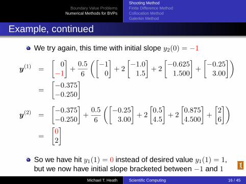
Example, continued

We try again, this time with initial slope y2(0) = −1

y(1) =[

0−1

]+

0.56

([−1

0

]+ 2

[−1.0

1.5

]+ 2

[−0.625

1.500

]+

[−0.25

3.00

])=

[−0.375−0.250

]

y(2) =[−0.375−0.250

]+

0.56

([−0.25

3.00

]+ 2

[0.54.5

]+ 2

[0.8754.500

]+

[26

])=

[02

]So we have hit y1(1) = 0 instead of desired value y1(1) = 1,but we now have initial slope bracketed between −1 and 1




Example, continued

We omit further iterations necessary to identify correctinitial slope, which turns out to be y2(0) = 0

y(1) =[00

]+

0.56

([00

]+ 2

[0.01.5

]+ 2

[0.3751.500

]+

[0.753.00

])=

[0.1250.750

]

y(2) =[0.1250.750

]+

0.56

([0.753.00

]+ 2

[1.54.5

]+ 2

[1.8754.500

]+

[36

])=

[13

]So we have indeed hit target solution value y1(1) = 1




Example, continued

< interactive example >


http://www.cse.uiuc.edu/iem/ode/shoot/



Multiple Shooting

Simple shooting method inherits stability (or instability) ofassociated IVP, which may be unstable even when BVP isstable

Such ill-conditioning may make it difficult to achieveconvergence of iterative method for solving nonlinearequation

Potential remedy is multiple shooting, in which interval [a, b]is divided into subintervals, and shooting is carried out oneach

Requiring continuity at internal mesh points provides BCfor individual subproblems

Multiple shooting results in larger system of nonlinearequations to solve




Finite Difference Method

Finite difference method converts BVP into system ofalgebraic equations by replacing all derivatives with finitedifference approximations

For example, to solve two-point BVP

u′′ = f(t, u, u′), a < t < b


we introduce mesh points ti = a + ih, i = 0, 1, . . . , n + 1,where h = (b− a)/(n + 1)

We already have y0 = u(a) = α and yn+1 = u(b) = β fromBC, and we seek approximate solution value yi ≈ u(ti) ateach interior mesh point ti, i = 1, . . . , n




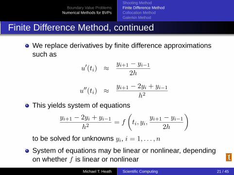
Finite Difference Method, continued

We replace derivatives by finite difference approximationssuch as

u′(ti) ≈ yi+1 − yi−1

2h

u′′(ti) ≈ yi+1 − 2yi + yi−1

h2

This yields system of equations

yi+1 − 2yi + yi−1

h2= f

(ti, yi,

yi+1 − yi−1

2h

)to be solved for unknowns yi, i = 1, . . . , n

System of equations may be linear or nonlinear, dependingon whether f is linear or nonlinear




Finite Difference Method, continued

For these particular finite difference formulas, system to besolved is tridiagonal, which saves on both work andstorage compared to general system of equations

This is generally true of finite difference methods: theyyield sparse systems because each equation involves fewvariables




Example: Finite Difference Method

Consider again two-point BVP

u′′ = 6t, 0 < t < 1

with BCu(0) = 0, u(1) = 1

To keep computation to minimum, we computeapproximate solution at one interior mesh point, t = 0.5, ininterval [0, 1]

Including boundary points, we have three mesh points,t0 = 0, t1 = 0.5, and t2 = 1

From BC, we know that y0 = u(t0) = 0 and y2 = u(t2) = 1,and we seek approximate solution y1 ≈ u(t1)




Example, continued

Replacing derivatives by standard finite differenceapproximations at t1 gives equation

y2 − 2y1 + y0

h2= f

(t1, y1,

y2 − y0

2h

)Substituting boundary data, mesh size, and right hand sidefor this example we obtain

1− 2y1 + 0(0.5)2

= 6t1

or4− 8y1 = 6(0.5) = 3

so thaty(0.5) ≈ y1 = 1/8 = 0.125




Example, continued

In a practical problem, much smaller step size and manymore mesh points would be required to achieve acceptableaccuracy

We would therefore obtain system of equations to solve forapproximate solution values at mesh points, rather thansingle equation as in this example



http://www.cse.uiuc.edu/iem/ode/findiff/



Collocation Method

Collocation method approximates solution to BVP by finitelinear combination of basis functions

For two-point BVP

u′′ = f(t, u, u′), a < t < b


we seek approximate solution of form

u(t) ≈ v(t, x) =n∑

i=1

xiφi(t)

where φi are basis functions defined on [a, b] and x isn-vector of parameters to be determined




Collocation Method

Popular choices of basis functions include polynomials,B-splines, and trigonometric functions

Basis functions with global support, such as polynomials ortrigonometric functions, yield spectral method

Basis functions with highly localized support, such asB-splines, yield finite element method




Collocation Method, continued

To determine vector of parameters x, define set of ncollocation points, a = t1 < · · · < tn = b, at whichapproximate solution v(t, x) is forced to satisfy ODE andboundary conditions

Common choices of collocation points includeequally-spaced points or Chebyshev points

Suitably smooth basis functions can be differentiatedanalytically, so that approximate solution and its derivativescan be substituted into ODE and BC to obtain system ofalgebraic equations for unknown parameters x




Example: Collocation Method

Consider again two-point BVP

u′′ = 6t, 0 < t < 1,

with BCu(0) = 0, u(1) = 1

To keep computation to minimum, we use one interiorcollocation point, t = 0.5

Including boundary points, we have three collocationpoints, t0 = 0, t1 = 0.5, and t2 = 1, so we will be able todetermine three parameters

As basis functions we use first three monomials, soapproximate solution has form

v(t, x) = x1 + x2t + x3t2




Example, continuedDerivatives of approximate solution function with respect tot are given by

v′(t, x) = x2 + 2x3t, v′′(t, x) = 2x3

Requiring ODE to be satisfied at interior collocation pointt2 = 0.5 gives equation

v′′(t2,x) = f(t2, v(t2,x), v′(t2,x))

or2x3 = 6t2 = 6(0.5) = 3

Boundary condition at t1 = 0 gives equation

x1 + x2t1 + x3t21 = x1 = 0

Boundary condition at t3 = 1 gives equation

x1 + x2t3 + x3t23 = x1 + x2 + x3 = 1




Example, continued

Solving this system of three equations in three unknownsgives

x1 = 0, x2 = −0.5, x3 = 1.5

so approximate solution function is quadratic polynomial

u(t) ≈ v(t, x) = −0.5t + 1.5t2

At interior collocation point, t2 = 0.5, we have approximatesolution value

u(0.5) ≈ v(0.5,x) = 0.125




Example, continued



http://www.cse.uiuc.edu/iem/ode/colloc/

scientiﬁc computing: an introductory survey value problems numerical methods for bvps boundary...

Documents