MNRAS 000, 1–13 (2017) Preprint 7 February 2018 Compiled using MNRAS LATEX style file v3.0

SDSS-IV MaNGA: Global stellar population and gradientsfor about 2000 early-type and spiral galaxies on themass-size plane

Hongyu Li1,2?, Shude Mao3,1,4, Michele Cappellari5, Junqiang Ge1, R. J. Long1,4,

Ran Li1,6, H.J. Mo7,3, Cheng Li3, Zheng Zheng1, Kevin Bundy8 Daniel Thomas9,

Joel R. Brownstein10, Alexandre Roman Lopes11, David R. Law12 and Niv Drory131National Astronomical Observatories, Chinese Academy of Sciences, 20A Datun Road, Chaoyang District, Beijing 100012, China2University of Chinese Academy of Sciences, Beijing 100049, China3Physics Department and Tsinghua Centre for Astrophysics, Tsinghua University, Beijing 100084, China4Jodrell Bank Centre for Astrophysics, School of Physics and Astronomy, The University of Manchester, Oxford Road, Manchester M13 9PL, UK5Sub-Department of Astrophysics, Department of Physics, University of Oxford, Denys Wilkinson Building, Keble Road, Oxford, OX1 3RH, UK6Key laboratory for Computational Astrophysics, National Astronomical Observatories, Chinese Academy of Sciences, Beijing, 100012, China7Department of Astronomy, University of Massachusetts, Amherst MA 01003-9305, USA8UCO/Lick Observatory, University of California, Santa Cruz, 1156 High St. Santa Cruz, CA 95064, USA9Institute of Cosmology & Gravitation, University of Portsmouth, Dennis Sciama Building, Portsmouth, PO1 3FX, UK10Department of Physics and Astronomy, University of Utah, 115 S. 1400 E., Salt Lake City, UT 84112, USA11Departamento de FAssica, Facultad de Ciencias, Universidad de La Serena, Cisternas 1200, La Serena, Chile12Space Telescope Science Institute, 3700 San Martin Drive, Baltimore, MD 21218, USA13McDonald Observatory, The University of Texas at Austin, 1 University Station, Austin, TX 78712, USA

Accepted 2018 February 2. Received 2018 January 15; in original form 2017 October 30

ABSTRACTWe perform full spectrum fitting stellar population analysis and Jeans Anisotropicmodelling (JAM) of the stellar kinematics for about 2000 early-type galaxies (ETGs)and spiral galaxies from the MaNGA DR14 sample. Galaxies with different morpholo-gies are found to be located on a remarkably tight mass plane which is close to theprediction of the virial theorem, extending previous results for ETGs. By examin-ing an inclined projection (‘the mass-size’ plane), we find that spiral and early-typegalaxies occupy different regions on the plane, and their stellar population properties(i.e. age, metallicity and stellar mass-to-light ratio) vary systematically along roughlythe direction of velocity dispersion, which is a proxy for the bulge fraction. Galaxieswith higher velocity dispersions have typically older ages, larger stellar mass-to-lightratios and are more metal rich, which indicates that galaxies increase their bulge frac-tions as their stellar populations age and become enriched chemically. The age andstellar mass-to-light ratio gradients for low-mass galaxies in our sample tend to bepositive (centre < outer), while the gradients for most massive galaxies are negative.The metallicity gradients show a clear peak around velocity dispersion log10 σe ≈ 2.0,which corresponds to the critical mass ∼ 3 × 1010M of the break in the mass-sizerelation. Spiral galaxies with large mass and size have the steepest gradients, whilethe most massive ETGs, especially above the critical mass Mcrit >∼ 2 × 1011M, whereslow rotator ETGs start dominating, have much flatter gradients. This may be due todifferences in their evolution histories, e.g. mergers.

Key words: galaxies: kinematics and dynamics - galaxies: formation - galaxies:evolution - galaxies: structure

? E-mail: hyli@nao.cas.cn

1 INTRODUCTION

Early-type galaxies (ETGs) have been found to follow sev-eral scaling relations, for example the fundamental plane

© 2017 The Authors

arX

iv:1

802.

0181

9v1

[as

tro-

ph.G

A]

6 F

eb 2

018

2 Li et al.

(Djorgovski & Davis 1987; Dressler et al. 1987), which de-scribes the relationship between velocity dispersion σ, ef-fective (half light) radius Re and luminosity L (or surfacebrightness µ). There are similar relationships for the stel-lar mass plane (Hyde & Bernardi 2009) and the mass plane(Cappellari et al. 2006; Bolton et al. 2007), in which the lu-minosity is replaced by stellar mass and total mass, respec-tively. These scaling relations are related to the viral theo-rem (Faber et al. 1987). The edge-on view of these planesare thin, especially for the mass plane (Auger et al. 2010;Cappellari et al. 2013a).

For the face-on view, however, galaxies with differentproperties may be located in different regions. Graves et al.(2009) and Graves & Faber (2010) studied the age, metallic-ity and mass-to-light ratio of the galaxies on the fundamen-tal plane using the SDSS (York et al. 2000) single fibre spec-trum of quiescent galaxies, and found there are systematicvariations of the stellar populations across the fundamentalplane. Springob et al. (2012) performed a similar investiga-tion using data from the 6dF galaxy survey.

With integral field unit (IFU) data, e.g. ATLAS3D (Cap-pellari et al. 2011), CALIFA (Sanchez et al. 2012), MAS-SIVE (Ma et al. 2014), SAMI (Bryant et al. 2015) andMaNGA (Bundy et al. 2015), one can estimate the dynam-ical mass much more accurately and study the mass planerelationship (e.g. Cappellari et al. 2013a). Cappellari et al.(2013b) and McDermid et al. (2015) studied the distributionof the mass-to-light ratio, angular momentum, stellar popu-lation and star formation history on the mass plane for the260 early-type galaxies in the ATLAS3D survey. They foundthe ages, metallicity, elemental abundance and gas contentof galaxies vary systematically on the mass-size plane (seeFig. 22 of Cappellari 2016).

Population gradients contain information on galaxy evo-lution, e.g. accretion, merger (Hopkins et al. 2009; Di Matteoet al. 2009) and radial migration (Roediger et al. 2012; Zhenget al. 2015). There are many previous studies focused on thegradients of galaxies, e.g. correlation between age, metal-licity gradients and galaxy properties such as stellar mass,colour, velocity dispersion (Mehlert et al. 2003; Sanchez-Blazquez et al. 2007; Koleva et al. 2009; Spolaor et al. 2009;MacArthur et al. 2009; Kuntschner et al. 2010; Tortora et al.2010; Rawle et al. 2010; La Barbera et al. 2012; Kuntschner2015) and environments (Sanchez-Blazquez et al. 2006b;Tortora & Napolitano 2012; Roediger et al. 2011; Zhenget al. 2017; Goddard et al. 2017).

In this paper, we use the galaxies from the MaNGADR14 (Abolfathi et al. 2017) sample, Jeans anisotropicmodel (JAM) (Cappellari 2008), and full spectrum fittingtechnique (pPXF, Cappellari & Emsellem 2004) to studythe distribution of the stellar population properties (i.e. age,metallicity, stellar mass-to-light ratio and their gradient) onthe mass-size plane (the projection along σ direction of themass plane) for galaxies with different morphologies. Thestructure of the paper is as follows. In Section 2, we de-scribe the MaNGA data (Section 2.1), dynamical modelling(Section 2.2) and stellar population synthesis model (Sec-tion 2.3). In Section 3, we show our results concerning themass plane relationship (Section 3.1), the distribution of theglobal population properties (Section 3.2) and the distribu-tion of the population gradients on the mass-size plane (Sec-tion 3.3). In Section 4, we summarize our results and draw

our conclusions. We make use of a flat ΛCDM cosmologywith Ωm = 0.315 and H0 = 67.3 km s−1 Mpc−1 (Planck Col-laboration et al. 2014).

2 DATA AND MODELS

2.1 MaNGA data and galaxy sample

The galaxies in this study are from the MaNGA ProductLaunch 5 (MPL5) catalogue (internal release, nearly iden-tical to SDSS-DR14, Abolfathi et al. 2017), which includes2778 galaxies of different morphologies. We base our galaxymorphologies on the Galaxy Zoo 1 (Lintott et al. 2008, 2011)by first matching the MPL5 sample with Table 2 of Lin-tott et al. (2011). For galaxies with uncertain flags or notin the table, we classify them by their Sersic index (Sersic1963) from the NASA-Sloan Atlas1 (NSA) catalogue whichis based on SDSS imaging (Blanton et al. 2011). We takegalaxies with nSersic > 2.5 as early type galaxies (ETGs)and the remainder as spiral galaxies. We then visually checkall the galaxies to adjust any misclassified galaxies and toexclude merging galaxies. Galaxies with low data quality(with fewer than 100 Voronoi bins with signal-to-noise, S/N,greater than 10) are also excluded. In total, we have 2110galaxies in our final sample, with 952 ETGs and 1158 spi-rals. In order to test the effect of morphology classification,we also examine our results using a subsample with inter-mediate sersic index (2 < nSersic < 3) excluded (932 spiralgalaxies and 898 ETGs in this subsample), and find thatour conclusions remain unchanged.

IFU spectra are extracted using the MaNGA data re-duction pipeline (Law et al. 2016), and kinematical data areextracted using the MaNGA data analysis pipeline (K. West-fall et al. 2017, in preparation). The data analysis pipelineextracts the kinematic data from the IFU spectra by fit-ting absorption lines using the pPXF software (Cappel-lari & Emsellem 2004; Cappellari 2017) with a subset ofthe MILES (Sanchez-Blazquez et al. 2006a; Falcon-Barrosoet al. 2011) stellar library, MILES-THIN. Before fitting, thespectra are Voronoi binned (Cappellari & Copin 2003) toS/N=10. Readers are referred to the following papers formore details on the MaNGA instrumentation (Drory et al.2015), observing strategy (Law et al. 2015), spectrophoto-metric calibration (Smee et al. 2013; Yan et al. 2016a), andsurvey execution and initial data quality (Yan et al. 2016b).

2.2 Dynamical modelling

We perform Jeans Anisotropic Modelling (JAM, Cappellari2008) for all the galaxies in our sample. The modelling al-lows for anisotropy in the second velocity moments. Thetotal mass model has two components, i.e. a stellar massdistribution and a dark halo. For the stellar component,we first use the Multi-Gaussian Expansion (MGE) method(Emsellem et al. 1994) with the fitting algorithm and Pythonsoftware2 by Cappellari (2002) to fit the SDSS r-band image.We then deproject the surface brightness to obtain the lu-minosity density and assume a constant stellar mass-to-light

1 http://www.nsatlas.org/data2 Available from http://purl.org/cappellari/software

MNRAS 000, 1–13 (2017)

Stellar population on the mass-size plane 3

0.4

0.2

0.0

0.2

0.4

[Z/H

]

NGC2549

0 5 10 15 20 25R [arcsec]

9.4

9.6

9.8

10.0

10.2

log 1

0Age

[yea

r]

0.4

0.2

0.0

0.2

0.4

[Z/H

]

This workKuntschner et al. (2010)

NGC4459

0 5 10 15 20 25 30R [arcsec]

9.4

9.6

9.8

10.0

10.2lo

g 10A

ge[y

ear]

0.45

0.30

0.15

0.00

0.15

[Z/H

]

NGC4473

0 5 10 15 20 25 30R [arcsec]

9.75

9.90

10.05

10.20

log 1

0Age

[yea

r]

0.30

0.15

0.00

0.15

0.30

[Z/H

]

NGC4526

0 5 10 15 20 25 30 35R [arcsec]

9.4

9.6

9.8

10.0

10.2

log 1

0Age

[yea

r]

0.50

0.25

0.00

0.25

[Z/H

]

NGC4564

0 5 10 15 20R [arcsec]

9.75

9.90

10.05

10.20

log 1

0Age

[yea

r]

0.30

0.15

0.00

0.15

0.30

[Z/H

]

NGC4621

0 5 10 15 20 25 30R [arcsec]

9.75

9.90

10.05

10.20

log 1

0Age

[yea

r]

0.75

0.50

0.25

0.00

0.25

[Z/H

]

NGC4660

0 5 10 15 20 25R [arcsec]

9.75

9.90

10.05

10.20lo

g 10A

ge[y

ear]

1

Figure 1. Comparison of the logAge and [Z/H] profiles for 7 galaxies with high S/N from the ATLAS3D survey. The blue symbols are

the results of each IFU bin from Kuntschner et al. (2010), using line indices based method. The red symbols are the results of each IFUbin using the full spectrum fitting method described in Section 2.3.

ratio to convert the light distribution to the stellar mass dis-tribution. For the dark matter halo, we assume a generalisedNFW (Navarro et al. 1996) halo profile

ρDM(r) = ρs(

rRs

)γ (12+

12

rRs

)−γ−3. (1)

From running JAM within an MCMC framework (emcee,Foreman-Mackey et al. 2013), we find the best-fitting param-eters which give the model best matching a galaxy’s observedsecond velocity moment map. The model gives a robust totalmass estimation as demonstrated in Lablanche et al. (2012)and Li et al. (2016) using numerical simulations. Details ofthe modelling procedures can be found in Li et al. (2016,2017).

Following Cappellari et al. (2013a), we calculate the size

parameters Re, Rmaje and r1/2 from the MGE models, and

scale the Re and Rmaje by a factor of 1.35 (see Fig. 7 of Cap-

pellari et al. 2013a). Here Re is the circularized effective ra-

dius, Rmaje is the major axis of the half-light isophote and r1/2

is the 3-dimensional half-light radius. We define M1/2 as theenclosed total mass within a spherical radius r1/2 from thebest fitting JAM models. The velocity dispersion σe is de-fined as the square-root of the luminosity-weighted averagesecond moments of the velocity within an elliptical apertureof area A = πR2

e

σe =

√∑k Fk (V2

k+ σ2

k)∑

k Fk(2)

where Vk and σk are the mean velocity and dispersion of theGaussian which best fits the line-of-sight velocity distribu-tion in the k-th IFU spaxel, and Fk is the flux in the k-th IFUspaxel. The sum is within the elliptical aperture described

above. The σe so defined agrees quite closely with the ve-locity dispersion measured from a single fit to the spectruminside the same aperture (Cappellari et al. 2013a).

2.3 Stellar population synthesis (SPS)

We estimate the stellar population properties by fitting theMaNGA IFU spectra with stellar population templates. Be-fore spectrum fitting, we remove spectra with signal-to-noiseratio (S/N) less than 5 and bad sky subtractions. The datacubes are then Voronoi binned (Cappellari & Copin 2003)to S/N=30. We also used S/N=60, and find that our results(age, metallity, stellar mass-to-light ratio and their gradi-ents) are nearly unchanged. The S/N for each spectrum iscalculated as the ratio between the mean and the standarddeviation of the flux within a window from 4730A to 4780A,which does not include obvious emission and absorptionlines. We use the pPXF software (Cappellari & Emsellem2004; Cappellari 2017) with the MILES-based (Sanchez-Blazquez et al. 2006a) SPS models of Vazdekis et al. (2010)and Salpeter (1955) initial mass function. We use 25 agesuniformly spaced in log10Age (years) between 7.8 and 10.25and 6 metallicities ([Z/H] = [-1.70, -1.30, -0.70, -0.40, 0.00,0.22]). We assume a Calzetti et al. (2000) reddening curveand do not allow for any polynomial and regularisation inthe fitting. The fitting is performed between ∼ 3500A and∼ 7400A. During the spectrum fitting we do not mask the gasemission lines in pPXF, but instead, we fit them simultane-ously to the stellar templates as Gaussians, while adoptingthe same kinematics for all the gas emission lines. We in-clude the emissions from the Balmer series, the [OIII], [NII]doublet (with a fixed ratio 1/3), the [OI] doublet (with a

MNRAS 000, 1–13 (2017)

4 Li et al.

9.0 9.5 10.0 10.5 11.0 11.5 12.0 12.5log10 2 × M1/2

9.0

9.5

10.0

10.5

11.0

11.5

12.0

12.5

a+bl

og10

e+cl

og10

Rmaj

e

a = 11.279 ± 0.0028b = 1.959 ± 0.018c = 0.964 ± 0.013

z = 0 ± 0= 0.047

(x0 = 2.247)(y0 = 0.7719)

Mass Plane (ETGs)

9.5 10.0 10.5 11.0 11.5 12.0log10 2 × M1/2

9.5

10.0

10.5

11.0

11.5

12.0

a+bl

og10

e+cl

og10

Rmaj

e

a = 10.6862 ± 0.0024b = 1.871 ± 0.015c = 0.948 ± 0.012

z = 0 ± 0= 0.061

(x0 = 1.905)(y0 = 0.8162)

Mass Plane (spiral)

1

Figure 2. The edge-on view of the best-fitting mass plane for theETGs (top) and the spiral galaxies (bottom) in our sample. The

coefficients of the best-fitting plane a+b(x− x0)+c(y−y0) and theobserved scatter ∆ in z are shown at upper left of each panel. Thered dashed lines show the 1σ (68%) and 2.6σ (99%). The outliers

excluded from the fit by the LTS PLANEFIT (Cappellari et al.

2013a) procedure are shown with green symbols.

fixed ratio 3/1), the [OII] and the [SII]. We fit every spec-trum twice. In the first pass, we fit all the good pixels andobtain the best fitting model spectrum. In the second pass,we remove all the pixels outside 3σ from the first fitting.We use the results from the second fitting in our followinganalysis.

We calculate the luminosity weighted log10Age andmetallicity [Z/H] using the equation below:

〈x〉 =∑N

j=1 wjLj xj∑Nj=1 wjLj

, (3)

where wj is the weight of the jth template and Lj is thecorresponding r-band luminosity of the SPS template. xj isthe log10Age (or [Z/H]) of the jth template when calculatingluminosity weighted log10Age (or [Z/H]). The stellar mass-to-light ratio is calculated as

M∗/L =∑N

j=1 wjMnogasj∑N

j=1 wjLj

, (4)

where Mnogasj

is the stellar mass of the jth template, which

includes the mass in living stars and stellar remnants, butexcludes the gas lost during stellar evolution. The other sym-bols are the same as in equation 3.

Having the log10Age, [Z/H] and M∗/L for each bin, wetake the luminosity weighted mean values within one effec-tive radius (an ellipse close to the half-light isophote) as theglobal population properties. For the gradients of these prop-erties, we first calculate the radial profiles of those quanti-ties by taking the median values in different elliptical annuli,with the global ellipticity measured around 1Re. We then fitthe profiles (logAge, [Z/H] and log10 M ∗ /L vs. log10 R/Re)between Re/8 and 1Re to obtain the linear slopes as our gra-dients. A negative gradient means the central value is largerthan the outer one.

To test the robustness of our approach and to get asense of the possible systematics, we apply our full spec-trum fitting method on 7 galaxies with high S/N from theATLAS3D survey, and compare our mettallicity and logAgeprofiles with the results from Kuntschner et al. (2010), whichare based on a radically different approach. The ATLAS3D

results are in fact obtained by measuring three line indices,correcting them to a uniform velocity dispersion and thenlocating the values, in a χ2 sense, on a 3-dimensional gridof individual SPS model predictions by Schiavon (2007), asa function of age, metallicity and alpha enhancement. Thecomparisons are shown in Fig. 1. As one can see, two meth-ods give comparable trends. Our results show small scat-ters since we use full spectrum fitting rather than just lineindices. At the centre, our metallicities are slightly lowerbecause our templates do not allow for non-solar abun-dances and in particular do not have [Z/H] > 0.22 as inKuntschner et al. (2010). Correspondingly, the central agesare slightly higher. Although the measurements were ob-tained with quite significant differences both in the SPSmodel and in the fitting method, the agreement is quitegood. In particular, the trends in both the age and the metal-licity gradients are consistent between the two approaches.

Throughout this work, we use the pPXF software com-bined with the MILES stellar template library to obtain thestellar populations in galaxies. As a cross-check, we havealso used the BC03 (Bruzual & Charlot 2003) SSP templatescombined with the pPXF. With reasonable regularization,the BC03 library gives similar results as the MILES tem-plate.

3 RESULTS

3.1 Mass plane

The mass plane relationship can be written as

log M1/2 = a + b logσe + c log Rmaje , (5)

where M1/2, σe and Rmaje are described in Section 2.2. The

expected values from the virial theorem are b = 2 andc = 1 (Faber et al. 1987). We fit this relationship sepa-rately for the ETGs and spiral galaxies in our sample, usingthe LST PLANEFIT procedure described in Cappellariet al. (2013a) which combines the Least Trimmed Squaresrobust technique of Rousseeuw & Van Driessen (2006) into aleast-squares fitting algorithm which allows for errors in all

MNRAS 000, 1–13 (2017)

Stellar population on the mass-size plane 5

variables and intrinsic scatter. In the fitting, we assume 6%error in σe, 6% in Rmaj

e and 10% error in M1/2 (Cappellariet al. 2013a). The results and the best fitting parameters areshown in Fig 2.

As one can see, both ETGs and spiral galaxies are on aremarkably tight mass plane, with coefficients b and c closeto the prediction from the virial theorem. This agrees withthe results of b = 1.942, c = 0.991 and ∆ = 0.077 in Cap-pellari et al. (2013b), and follow the virial theorem slightlybetter than the results of b = 1.67, c = 1.04, ∆ = 0.059 fromScott et al. (2015) and α = 1.857, β = −1.279 in Auger et al.(2010), with α = 2, β = −1 being the prediction from thevirial theorem in their formalism. The observed scatter ∆for spiral galaxies is 0.061, which is slightly larger than thevalue 0.047 for the ETGs. This is because the uncertaintiesin measuring the velocity dispersion, effective radius anddynamical mass are larger for spiral galaxies due to the lim-ited spectral resolution, the asymmetry of the galaxy andperturbation of the spiral arms. In the current data analysispipeline for stellar kinematics, the extracted velocity dis-persions under 50 km s−1 have larger scatters, and may beslightly overestimated due to the uncertainties of the instru-mental resolution. This may account for the slightly largerdeviation of the mass plane coefficients from the virial theo-rem for the spiral galaxies. The intrinsic scatters εz for bothETGs and spiral galaxies are consistent with being 0, untilwe reduce the error for the measured quantities in the fitting

to 5% (σe), 5% (Rmaje ) and 3% (M1/2). In the following sec-

tions, we use the ‘mass-size plane’ to refer to the projectionof the mass plane along the σe direction. We choose this pro-jection because it is close to face-on and the two axes haveclear physical meanings (i.e. mass and size).

3.2 Stellar population on the mass-size plane

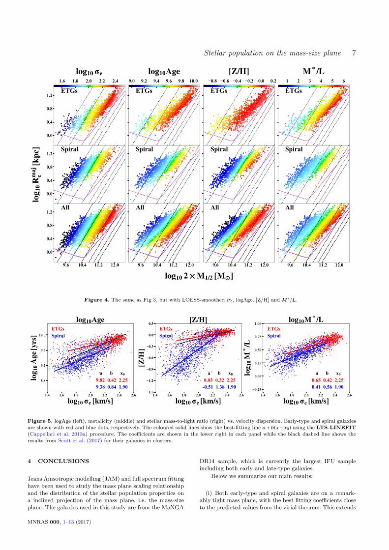
We estimate the stellar population properties for all thegalaxies in our sample using the full spectrum fitting methoddescribed in Section 2.3. The distributions of the veloc-ity dispersions, ages, metallicities and stellar mass-to-lightratios of these galaxies on the mass-size plane are shownin Fig. 3. We use the Python implementation3 (Cappellariet al. 2013b) of the two-dimensional Locally Weighted Re-gression (LOESS, Cleveland & Devlin 1988) method to ob-tain smoothed distributions, which are shown in Fig.4. Thevelocity dispersions on the mass-size plane agree well withthe prediction from the virial theorem, as indicated by theblack dashed lines. The age, the metallicity and the stellarmass-to-light ratio change systematically on the mass-sizeplane for both ETGs and spiral galaxies. The values increaseroughly along the velocity dispersion direction, which tracethe bulge mass fraction (Cappellari 2016). These systematictrends of the stellar population with velocity dispersion areconsistent with a picture in which the bulge growth makesthe population more metal rich and increases the likelihoodfor the star formation to be quenched (see Fig. 23 of Cap-pellari 2016).

In a very recent work, Scott et al. (2017) showed similarresults for ∼ 1300 galaxies with different morphologies from

3 Available from http://purl.org/cappellari/software

the SAMI IFU survey. Other than our sample being slightlylarger (2110 vs. 1300), our two studies differ in four aspects

(i) Their stellar population properties are derived fromline indices, rather than full spectrum fitting as in our study;

(ii) They use stellar mass while we use dynamical mass;(iii) They study the galaxy global properties only while

we study both global properties and gradients in the stellarpopulations (see Section 3.3).

(iv) Finally, the two studies are based on quite differentsamples, observed with different IFUs, and analyzed withdifferent data pipelines.

The 1-dimensional relationship between velocity disper-sion and age, metallicity and stellar mass-to-light ratio areshown in Fig. 5. We fit the relationship using the equationbelow for ETGs and spiral galaxies

y = a + b(x − x0), (6)

where x0 is the median value of x. The best fitting line andcoefficients are shown in each panel of Fig. 5. The resultsfrom Scott et al. (2017) for their galaxies in clusters areshown in Fig. 5 with black dashed lines. Their fitting didnot separate ETGs and spiral galaxies. Unlike Fig. 5 of Scottet al. (2017), our logAge–velocity dispersion relation showssimilar bimodality to the metallicity–velocity dispersion re-lation, and their [Z/H] reaches values as low as −2, while inour results the values never go below −1.4.

3.3 Stellar population gradient on the mass-sizeplane

We use the method described in Section 2.3 to estimate theage, metallicity and stellar mass-to-light ratio gradients forthe galaxies in our sample. Similar to Figs. 3 and 4, we showthe distribution of these gradients on the mass-size plane inFigs. 6 and 7. The systematic trends for the gradients arenot as simple as the global properties which vary monotoni-cally with the velocity dispersion as in Fig. 3, but there areseveral special features for the distribution of the populationgradients on the mass-size plane

(i) Many galaxies with small size and mass have positiveage and stellar mass-to-light ratio gradient (centre < outer),which may be due to the star formation in galaxy centre(Huang et al. 1996; Ellison et al. 2011; Oh et al. 2012), whilenearly all the galaxies with log10 2 × M1/2 > 11.2 have neg-ative age and stellar mass-to-light ratio gradients. The ageand the stellar mass-to-light ratio gradients for ETGs arecorrelated with galaxy mass.

(ii) The metallicity gradients for spiral galaxies increase(become more negative) with mass and size, while forETGs, the metallicity gradients change with velocity dis-persions. ETGs with higher and lower velocity dispersionshave slightly shallower gradients.

(iii) Spiral galaxies with large size and mass have thesteepest age, metallicity and stellar mass-to-light ratio gradi-ents. Although these galaxies are close to the massive ETGson the mass-size plane, their gradient properties have signifi-cant differences. One can see a clear boundary between thesetwo galaxy populations in Fig. 7, especially for the metal-licity gradient. This may be due to the differences in theirevolution histories, e.g. massive ETGs tend to have more

MNRAS 000, 1–13 (2017)

6 Li et al.

0.0

0.4

0.8

1.2ETGs

log10 e

ETGs

log10Age

ETGs

[Z/H]

ETGs

M * /L

0.0

0.4

0.8

1.2

log 1

0Rm

aje

[kpc

] Spiral Spiral Spiral Spiral

9.6 10.4 11.2 12.0

0.0

0.4

0.8

1.2All

9.6 10.4 11.2 12.0

log10 2 × M1/2 [M ]

All

9.6 10.4 11.2 12.0

All

9.6 10.4 11.2 12.0

All

1.6 1.8 2.0 2.2 2.4 9.0 9.2 9.4 9.6 9.8 10.0 1.2 1.0 0.8 0.6 0.4 0.2 0.0 0.2 1 2 3 4 5 6

Figure 3. Velocity dispersion σe, logAge, metalicity [Z/H] and stellar mass-to-light ratio M∗/L (SDSS r-band) distribution on the

mass-size plane (Rmaje vs. dynamical mass M1/2). Colours indicate the parameters as labelled at the top of each column. The results for

early-type, spiral and all galaxies are shown in the upper, middle and bottom panels, respectively. In the bottom panels, coloured squares

represent spiral galaxies and coloured circles represent ETGs. In each panel, dashed lines show lines of constant velocity dispersion: 50,

100, 200, 300, 400, and 500 km s−1 from left to right, as implied by the virial theorem. The magenta curve shows the zone of exclusiondefined in Cappellari et al. (2013b).

mergers (Cappellari 2016). This also agree with the scenariothat many of them are slow rotators (Graham et al. 2017,in preparation), which are thought to be formed by mergers(Naab et al. 2014; Penoyre et al. 2017; Li et al. 2018).

Here we note that our stellar mass-to-light gradients arebased on the assumption of a constant Salpeter (1955) stel-lar initial mass function (IMF). The results will not be af-fected by the global variation of the IMF (e.g. Conroy & vanDokkum 2012, Cappellari et al. 2012, Li et al. 2017), but by agradient of the IMF within galaxies (e.g. van Dokkum et al.2017 for massive elliptical galaxies). The age and metallicitygradients will not be affected by the IMF.

In Fig. 8, we plot the histogram of the age, metallicityand stellar mass-to-light ratio gradients and their relationwith velocity dispersions. One can see that the age and themetallicity gradients peak around logσe = 2.0 (especiallyfor metallicity gradients), which roughly corresponds to thecritical mass ∼ 3×1010M of the break in the mass-size rela-tion (Cappellari 2016), below which no fully passive ETGsexist. The same critical mass is also shown in Kauffmannet al. (2003). This agree well with the results in Spolaoret al. (2009), Tortora et al. (2010), Kuntschner et al. (2010)

and Kuntschner (2015), but is slightly different from the re-sults in Goddard et al. (2017), which did not show a cleardecrease of the metallicity gradients with increasing stellarmasses. The galaxies in our sample occupy similar regionof the metallicity – velocity dispersion relationship with thesimulated galaxies in Hopkins et al. (2009). We also con-struct Figs 6, 7 and 8 with intermediate Sersic index (2-3)galaxies excluded, and find no significant differences fromthe main sample.

In Fig. 9, to visually illustrate and confirm the realityof the the statistical results of Figs. 6 and 7, we show themetallicity profiles between Re/8 and 1Re of some galaxieswith the best data qualities on the mass-size plane. Theselected galaxies have more than 400 Voronoi bins with S/Ngreater than 30 for the top 4 rows in Fig. 9, and more than200 Voronoi bins for the bottom row because small galaxieshave lower data qualities. The spiral galaxies with large sizeand mass have very steep metallicity gradients, while thegradients for massive eliiptical galaxies are much shallower.

MNRAS 000, 1–13 (2017)

Stellar population on the mass-size plane 7

0.0

0.4

0.8

1.2ETGs

log10 e

ETGs

log10Age

ETGs

[Z/H]

ETGs

M * /L

0.0

0.4

0.8

1.2

log 1

0Rm

aje

[kpc

] Spiral Spiral Spiral Spiral

9.6 10.4 11.2 12.0

0.0

0.4

0.8

1.2All

9.6 10.4 11.2 12.0

log10 2 × M1/2 [M ]

All

9.6 10.4 11.2 12.0

All

9.6 10.4 11.2 12.0

All

1.6 1.8 2.0 2.2 2.4 9.0 9.2 9.4 9.6 9.8 10.0 0.8 0.6 0.4 0.2 0.0 0.2 1 2 3 4 5 6

Figure 4. The same as Fig 3, but with LOESS-smoothed σe, logAge, [Z/H] and M∗/L.

1.4 1.6 1.8 2.0 2.2 2.4 2.6

log10 e [km/s]

8.8

9.2

9.6

10.0

log 1

0Ag

e[yr

s]

ETGsSpiral

a b x0 9.82 0.42 2.25 9.38 0.84 1.90

log10Age

1.4 1.6 1.8 2.0 2.2 2.4 2.6

log10 e [km/s]1.5

1.2

0.9

0.6

0.3

0.0

0.3

[Z/H

]

ETGsSpiral

a b x0 0.03 0.32 2.25-0.51 1.38 1.90

[Z/H]

1.4 1.6 1.8 2.0 2.2 2.4 2.6

log10 e [km/s]0.25

0.00

0.25

0.50

0.75

1.00

log 1

0M

* /L

ETGsSpiral

a b x0 0.65 0.42 2.25 0.41 0.56 1.90

log10M * /L

Figure 5. logAge (left), metalicity (middle) and stellar mass-to-light ratio (right) vs. velocity dispersion. Early-type and spiral galaxies

are shown with red and blue dots, respectively. The coloured solid lines show the best-fitting line a + b(x − x0) using the LTS LINEFIT(Cappellari et al. 2013a) procedure. The coefficients are shown in the lower right in each panel while the black dashed line shows the

results from Scott et al. (2017) for their galaxies in clusters.

4 CONCLUSIONS

Jeans Anisotropic modelling (JAM) and full spectrum fittinghave been used to study the mass plane scaling relationshipand the distribution of the stellar population properties ona inclined projection of the mass plane, i.e. the mass-sizeplane. The galaxies used in this study are from the MaNGA

DR14 sample, which is currently the largest IFU sampleincluding both early and late-type galaxies.

Below we summarize our main results:

(i) Both early-type and spiral galaxies are on a remark-ably tight mass plane, with the best fitting coefficients closeto the predicted values from the virial theorem. This extends

MNRAS 000, 1–13 (2017)

8 Li et al.

0.0

0.4

0.8

1.2ETGs

log10Age

ETGs

[Z/H]

ETGs

log10M * /L

0.0

0.4

0.8

1.2

log 1

0Rm

aje

[kpc

] Spiral Spiral Spiral

9.6 10.4 11.2 12.0

0.0

0.4

0.8

1.2All

9.6 10.4 11.2 12.0

log10 2 × M1/2 [M ]

All

9.6 10.4 11.2 12.0

All

0.6 0.4 0.2 0.0 0.2 0.6 0.4 0.2 0.0 0.2 0.4 0.3 0.2 0.1 0.0 0.1

Figure 6. Age, metallicity and stellar mass-to-light ratio gradient (∆logAge, ∆[Z/H] and ∆M∗/L) distribution on the mass-size plane.

The gradients are defined in Section 2.3. A positive ∆ value indicates a positive gradient, i.e. the central value is higher. Other labels are

the same as in Fig 3.

the previous result for ETGs population to the whole galaxypopulation.

(ii) The stellar population properties (i.e. age, metallicityand stellar mass-to-light ratio) of the galaxies in our samplevary systematically on the mass-size plane along roughly thevelocity dispersion direction. The stellar population of thegalaxies with higher velocity dispersion are older and moremetal rich, which are consistent with a picture in which thebulge growth makes the population more metal rich andincreases the likelihood for the star formation to be quenched(Cappellari 2016).

(iii) The gradients of age and stellar mass-to-light ratiocould be positive (centre < outer) for low mass galaxies, whilemost massive galaxies have negative gradient.

(iv) The metallicity-velocity dispersion relation shows aclear peck around logσe ≈ 2.0, which corresponds to thecritical mass ∼ 3×1010M of the break in the mass-size rela-tion (Cappellari 2016), below which no fully passive ETGsexist.

(v) The distribution of the population gradients on the

mass-size plane shows a clear boundary between massivespiral and early-type galaxies. Spiral galaxies with large sizeand mass have the steepest gradients. In contrast, the mas-sive ETGs located in similar region have shallower gradients.This may be due to differences in their evolution histories,e.g. mergers.

The trends we see in this work, particularly the gradientsshown in Figs. 6 and 7, are puzzling and warrant furtherstudies. Observationally, these trends are still subject to theage-metallicity degeneracy and the scatters are still some-what high. Theoretically, the spatial resolutions in numericalsimulations and the treatments of physical processes, suchas the chemical enrichment and feedback processes, will af-fect the final predictions of the stellar populations and theirgradients. For example, according to Taylor & Kobayashi(2017) the metallicity gradients are affected by the initialsteep gradients from gas-rich assembly, passive evolution bystar formation and accretion at outskirts and flattening bymergers (major and minor). In reality, all these processes

MNRAS 000, 1–13 (2017)

Stellar population on the mass-size plane 9

0.0

0.4

0.8

1.2ETGs

log10Age

ETGs

[Z/H]

ETGs

log10M * /L

0.0

0.4

0.8

1.2

log 1

0Rm

aje

[kpc

] Spiral Spiral Spiral

9.6 10.4 11.2 12.0

0.0

0.4

0.8

1.2All

9.6 10.4 11.2 12.0

log10 2 × M1/2 [M ]

All

9.6 10.4 11.2 12.0

All

0.4 0.3 0.2 0.1 0.0 0.1 0.2 0.4 0.3 0.2 0.1 0.0 0.1 0.2 0.1 0.0 0.1

Figure 7. The same as Fig 6, but with LOESS-smoothed ∆logAge, ∆[Z/H] and ∆M∗/L.

may be operating at the same time, and it will take furtherefforts to decode the information we assembled here. Moredetailed comparisons with high-resolution cosmological sim-ulations such as Illustris (Vogelsberger et al. 2014a,b) andEAGLE (Schaller et al. 2015) may be a fruitful next step.

ACKNOWLEDGEMENTS

We thank Harald Kuntschner for providing the stellar popu-lation profiles for the 7 selected galaxies from the ATLAS3D

survey and the referee for helpful comments. MC acknowl-edges support from a Royal Society University Research Fel-lowship. We performed our computer runs on the Zen highperformance computer cluster of the National AstronomicalObservatories, Chinese Academy of Sciences (NAOC), andthe Venus server at Tsinghua University. This work was sup-ported by the National Science Foundation of China (GrantNo. 11333003, 11390372 to SM). This research made useof Marvin, a core Python package and web framework forMaNGA data, developed by Brian Cherinka, Jose Sanchez-Gallego, and Brett Andrews. (MaNGA Collaboration, 2017).

Funding for the Sloan Digital Sky Survey IV has beenprovided by the Alfred P. Sloan Foundation, the U.S. De-partment of Energy Office of Science, and the ParticipatingInstitutions. SDSS-IV acknowledges support and resourcesfrom the Center for High-Performance Computing at theUniversity of Utah. The SDSS web site is www.sdss.org.

SDSS-IV is managed by the Astrophysical ResearchConsortium for the Participating Institutions of the SDSSCollaboration including the Brazilian Participation Group,the Carnegie Institution for Science, Carnegie Mellon Uni-versity, the Chilean Participation Group, the French Par-ticipation Group, Harvard-Smithsonian Center for Astro-physics, Instituto de Astrofısica de Canarias, The JohnsHopkins University, Kavli Institute for the Physics andMathematics of the Universe (IPMU) / University of Tokyo,Lawrence Berkeley National Laboratory, Leibniz Institut furAstrophysik Potsdam (AIP), Max-Planck-Institut fur As-tronomie (MPIA Heidelberg), Max-Planck-Institut fur As-trophysik (MPA Garching), Max-Planck-Institut fur Ex-traterrestrische Physik (MPE), National Astronomical Ob-servatories of China, New Mexico State University, New

MNRAS 000, 1–13 (2017)

10 Li et al.

1.5 2.0 2.5log10 e [km/s]

1.0

0.5

0.0

0.5

log 1

0Ag

e

1.5 2.0 2.5log10 e [km/s]

1.0

0.5

0.0

0.5

[Z/H

]

1.5 2.0 2.5log10 e [km/s]

0.4

0.2

0.0

0.2

log 1

0M

* /L

1.0 0.5 0.0 0.5log10 Age

0

50

100

150

200

Num

ber

of g

alax

ies

0.081+0.1430.126

0.162+0.1960.224

1.0 0.5 0.0 0.5[Z/H]

0

50

100

150

200

Num

ber

of g

alax

ies

0.101+0.1190.150

0.164+0.2180.252

0.4 0.2 0.0 0.2log10 M * /L

0

50

100

150

Num

ber

of g

alax

ies

0.084+0.0880.088

0.090+0.1050.128

Figure 8. Top: gradients of logAge (left), metalicity (middle) and stellar mass-to-light ratio (right) vs. velocity dispersion. Early-type

and spiral galaxies are shown with red and blue dots, respectively. The green error bars show the median and scatter of all the galaxiesin each bin, calculated as the 16th, 50th and 84th percentiles. In the middle panel, black stars are the results from Kuntschner (2015),

the pink dashed line shows the trend from Spolaor et al. (2009) while the yellow shaded region shows the galaxy distribution from thesimulation Hopkins et al. (2009). Bottom: distribution of the logAge (left), metalicity (middle) and stellar mass-to-light ratio (right)

gradients for the early-type and spiral galaxies. The medians and 1σ scatters of the distributions are shown in each panel.

9.6 10.4 11.2 12.0log10 2 × M1/2 [M ]

0.0

0.4

0.8

1.2

log 1

0Rm

aje

[kpc

]

1.0 0.5 0.0log10R/Re

0.40.20.00.2

[Z/H

] 0.0-0.1

-0.3-0.5

Figure 9. Metallicity profiles ([Z/H] vs. log10 R/Re) for the selected high S/N galaxies in different regions of the mass-size plane. Blue

lines are the profiles for the spiral galaxies, red lines are for the ETGs. In each panel, the black solid lines represent the gradient valuesof 0, −0.1, −0.3 and −0.5, respectively. All the panels have the same scales as shown in the upper left panel. All the profiles have beenshifted to be 0 at Re/8.

MNRAS 000, 1–13 (2017)

Stellar population on the mass-size plane 11

York University, University of Notre Dame, ObservatarioNacional / MCTI, The Ohio State University, Pennsylva-nia State University, Shanghai Astronomical Observatory,United Kingdom Participation Group, Universidad NacionalAutonoma de Mexico, University of Arizona, Universityof Colorado Boulder, University of Oxford, University ofPortsmouth, University of Utah, University of Virginia, Uni-versity of Washington, University of Wisconsin, VanderbiltUniversity, and Yale University.

REFERENCES

Abolfathi B., et al., 2017, preprint, (arXiv:1707.09322)

Auger M. W., Treu T., Bolton A. S., Gavazzi R., KoopmansL. V. E., Marshall P. J., Moustakas L. A., Burles S., 2010,

ApJ, 724, 511

Blanton M. R., Kazin E., Muna D., Weaver B. A., Price-WhelanA., 2011, AJ, 142, 31

Bolton A. S., Burles S., Treu T., Koopmans L. V. E., MoustakasL. A., 2007, ApJ, 665, L105

Bruzual G., Charlot S., 2003, MNRAS, 344, 1000

Bryant J. J., et al., 2015, MNRAS, 447, 2857

Bundy K., et al., 2015, ApJ, 798, 7

Calzetti D., Armus L., Bohlin R. C., Kinney A. L., Koornneef J.,

Storchi-Bergmann T., 2000, ApJ, 533, 682

Cappellari M., 2002, MNRAS, 333, 400

Cappellari M., 2008, MNRAS, 390, 71

Cappellari M., 2016, ARA&A, 54, 597

Cappellari M., 2017, MNRAS, 466, 798

Cappellari M., Copin Y., 2003, MNRAS, 342, 345

Cappellari M., Emsellem E., 2004, PASP, 116, 138

Cappellari M., et al., 2006, MNRAS, 366, 1126

Cappellari M., et al., 2011, MNRAS, 413, 813

Cappellari M., et al., 2012, Nature, 484, 485

Cappellari M., et al., 2013a, MNRAS, 432, 1709

Cappellari M., et al., 2013b, MNRAS, 432, 1862

Cleveland W. S., Devlin S. J., 1988, Journal of the Americanstatistical association, 83, 596

Conroy C., van Dokkum P. G., 2012, ApJ, 760, 71

Di Matteo P., Pipino A., Lehnert M. D., Combes F., Semelin B.,

2009, A&A, 499, 427

Djorgovski S., Davis M., 1987, ApJ, 313, 59

Dressler A., Lynden-Bell D., Burstein D., Davies R. L., Faber

S. M., Terlevich R., Wegner G., 1987, ApJ, 313, 42

Drory N., et al., 2015, AJ, 149, 77

Ellison S. L., Nair P., Patton D. R., Scudder J. M., Mendel J. T.,Simard L., 2011, MNRAS, 416, 2182

Emsellem E., Monnet G., Bacon R., 1994, A&A, 285, 723

Faber S. M., Dressler A., Davies R. L., Burstein D., Lynden-BellD., 1987, in Faber S. M., ed., Nearly Normal Galaxies. Fromthe Planck Time to the Present. pp 175–183

Falcon-Barroso J., Sanchez-Blazquez P., Vazdekis A., RicciardelliE., Cardiel N., Cenarro A. J., Gorgas J., Peletier R. F., 2011,A&A, 532, A95

Foreman-Mackey D., Hogg D. W., Lang D., Goodman J., 2013,PASP, 125, 306

Goddard D., et al., 2017, MNRAS, 465, 688

Graves G. J., Faber S. M., 2010, ApJ, 717, 803

Graves G. J., Faber S. M., Schiavon R. P., 2009, ApJ, 698, 1590

Hopkins P. F., Cox T. J., Dutta S. N., Hernquist L., Kormendy

J., Lauer T. R., 2009, ApJS, 181, 135

Huang J. H., Gu Q. S., Su H. J., Hawarden T. G., Liao X. H.,

Wu G. X., 1996, A&A, 313, 13

Hyde J. B., Bernardi M., 2009, MNRAS, 396, 1171

Kauffmann G., et al., 2003, MNRAS, 341, 54

Koleva M., Prugniel P., De Rijcke S., Zeilinger W. W., Michielsen

D., 2009, Astronomische Nachrichten, 330, 960

Kuntschner H., 2015, in Cappellari M., Courteau S., eds, IAU

Symposium Vol. 311, Galaxy Masses as Constraints of For-mation Models. pp 53–56, doi:10.1017/S1743921315003385

Kuntschner H., et al., 2010, MNRAS, 408, 97

La Barbera F., Ferreras I., de Carvalho R. R., Bruzual G., Charlot

S., Pasquali A., Merlin E., 2012, MNRAS, 426, 2300

Lablanche P.-Y., et al., 2012, MNRAS, 424, 1495

Law D. R., et al., 2015, AJ, 150, 19

Law D. R., et al., 2016, AJ, 152, 83

Li H., Li R., Mao S., Xu D., Long R. J., Emsellem E., 2016,

MNRAS, 455, 3680

Li H., et al., 2017, ApJ, 838, 77

Li H., Mao S., Emsellem E., Xu D., Springel V., Krajnovic D.,2018, MNRAS, 473, 1489

Lintott C. J., et al., 2008, MNRAS, 389, 1179

Lintott C., et al., 2011, MNRAS, 410, 166

Ma C.-P., Greene J. E., McConnell N., Janish R., Blakeslee J. P.,

Thomas J., Murphy J. D., 2014, ApJ, 795, 158

MacArthur L. A., Gonzalez J. J., Courteau S., 2009, MNRAS,395, 28

McDermid R. M., et al., 2015, MNRAS, 448, 3484

Mehlert D., Thomas D., Saglia R. P., Bender R., Wegner G., 2003,

A&A, 407, 423

Naab T., et al., 2014, MNRAS, 444, 3357

Navarro J. F., Frenk C. S., White S. D. M., 1996, ApJ, 462, 563

Oh S., Oh K., Yi S. K., 2012, ApJS, 198, 4

Penoyre Z., Moster B. P., Sijacki D., Genel S., 2017, MNRAS,468, 3883

Planck Collaboration et al., 2014, A&A, 571, A16

Rawle T. D., Smith R. J., Lucey J. R., 2010, MNRAS, 401, 852

Roediger J. C., Courteau S., MacArthur L. A., McDonald M.,

2011, MNRAS, 416, 1996

Roediger J. C., Courteau S., Sanchez-Blazquez P., McDonald M.,2012, ApJ, 758, 41

Rousseeuw P. J., Van Driessen K., 2006, Data mining and knowl-edge discovery, 12, 29

Salpeter E. E., 1955, ApJ, 121, 161

Sanchez-Blazquez P., et al., 2006a, MNRAS, 371, 703

Sanchez-Blazquez P., Gorgas J., Cardiel N., 2006b, A&A, 457,

823

Sanchez-Blazquez P., Forbes D. A., Strader J., Brodie J., Proctor

R., 2007, MNRAS, 377, 759

Sanchez S. F., et al., 2012, A&A, 538, A8

Schaller M., et al., 2015, MNRAS, 452, 343

Schiavon R. P., 2007, ApJS, 171, 146

Scott N., et al., 2015, MNRAS, 451, 2723

Scott N., et al., 2017, preprint, (arXiv:1708.06849)

Sersic J. L., 1963, Boletin de la Asociacion Argentina de Astrono-

mia La Plata Argentina, 6, 41

Smee S. A., et al., 2013, AJ, 146, 32

Spolaor M., Proctor R. N., Forbes D. A., Couch W. J., 2009, ApJ,

691, L138

Springob C. M., et al., 2012, MNRAS, 420, 2773

Taylor P., Kobayashi C., 2017, MNRAS, 471, 3856

Tortora C., Napolitano N. R., 2012, MNRAS, 421, 2478

Tortora C., Napolitano N. R., Cardone V. F., Capaccioli M., Jet-zer P., Molinaro R., 2010, MNRAS, 407, 144

Vazdekis A., Sanchez-Blazquez P., Falcon-Barroso J., CenarroA. J., Beasley M. A., Cardiel N., Gorgas J., Peletier R. F.,

2010, MNRAS, 404, 1639

Vogelsberger M., et al., 2014a, MNRAS, 444, 1518

Vogelsberger M., et al., 2014b, Nature, 509, 177

Yan R., et al., 2016a, AJ, 151, 8

Yan R., et al., 2016b, AJ, 152, 197

York D. G., et al., 2000, AJ, 120, 1579

Zheng Z., et al., 2015, ApJ, 800, 120

MNRAS 000, 1–13 (2017)

12 Li et al.

Zheng Z., et al., 2017, MNRAS, 465, 4572

van Dokkum P., Conroy C., Villaume A., Brodie J., Romanowsky

A. J., 2017, ApJ, 841, 68

APPENDIX A: EXAMPLE DATA TABLE

MNRAS 000, 1–13 (2017)

Stellar population on the mass-size plane 13

Table A1. Properties of all the galaxies in the sample

MaNGA ID Morphology log10 σe log10 M1/2 log10 Rmaje log10 Age [Z/H] log10 M∗/Lr ∆ log10 Age ∆[Z/H] ∆ log10 M∗/Lr

(km s−1) (M) (kpc) (years) (M/Lr)(1) (2) (3) (4) (5) (6) (7) (8) (9) (10) (11)

1-320664 S 2.17 10.66 0.76 9.95 0.06 0.75 -0.15 0.14 -0.08

1-321069 E 2.37 11.48 1.07 9.80 0.14 0.66 -0.12 -0.05 -0.12

1-235587 E 2.04 10.27 0.50 9.66 0.06 0.54 0.04 -0.33 -0.041-320677 E 2.27 11.41 1.14 9.70 0.12 0.60 -0.38 0.18 -0.30

1-235576 S 2.10 10.82 0.75 9.74 -0.57 0.68 -0.04 0.45 -0.14

1-235530 E 2.22 10.53 0.41 9.90 0.07 0.73 -0.33 -0.15 -0.281-235398 S 2.10 10.67 0.78 9.71 -0.21 0.57 0.13 -0.10 0.06

1-320606 S 1.86 10.46 0.93 9.04 -0.86 0.21 -0.43 -0.55 -0.31

1-321074 E 2.27 11.04 0.83 9.64 0.15 0.56 -0.10 -0.09 -0.101-235582 E 1.84 9.92 0.58 9.33 0.07 0.30 0.31 -0.20 0.26

1-320584 E 2.47 11.70 1.08 9.94 0.12 0.77 -0.19 -0.06 -0.161-235611 S 2.06 11.00 1.11 9.56 -0.15 0.56 -0.68 -0.52 -0.39

1-320655 E 2.37 11.25 0.78 9.85 0.12 0.70 -0.23 0.00 -0.16

1-24092 E 2.13 10.37 0.35 9.01 -0.73 0.42 0.08 -0.28 0.351-23979 E 2.00 10.25 0.53 9.59 -0.10 0.53 0.02 -0.22 -0.01

1-24099 E 2.07 10.23 0.38 9.68 0.10 0.57 -0.11 -0.17 -0.08

1-23929 S 1.80 10.25 0.83 9.34 -0.52 0.41 -0.41 -0.12 -0.081-24368 S 1.72 9.96 0.77 9.19 -0.76 0.20 -0.14 0.06 -0.33

1-24354 S 1.75 9.87 0.51 9.83 -0.26 0.56 -0.14 0.10 -0.07

1-595027 S 2.05 10.72 0.90 9.24 -0.75 0.48 -0.25 -0.72 -0.041-595093 S 2.17 10.99 1.03 9.66 -0.02 0.64 -0.40 -0.13 -0.19

1-24018 E 2.11 10.58 0.71 9.78 0.07 0.64 -0.11 -0.22 -0.14

1-23891 S 2.20 10.82 0.78 9.80 0.03 0.66 -0.26 0.06 -0.181-24148 S 2.10 10.61 0.71 9.81 0.05 0.69 -0.19 0.10 -0.13

1-25937 S 2.22 11.34 1.22 9.70 -0.00 0.60 -0.36 -0.39 -0.251-25911 E 2.37 11.57 1.14 9.72 0.09 0.59 -0.24 -0.09 -0.23

1-24124 S 1.68 9.74 0.53 9.43 0.04 0.43 0.06 0.07 -0.02

1-115062 E 2.12 10.02 0.00 9.80 0.11 0.65 -0.00 0.04 -0.021-114928 E 2.24 10.76 0.67 9.91 -0.02 0.71 -0.12 -0.31 -0.19

1-115128 S 1.99 10.70 0.94 9.23 -0.59 0.34 -0.16 -0.50 -0.15

Note. — Column (1): The MaNGA ID of the galaxy. Column (2): Galaxy morphology. E for ETGs, S for spiral galaxies. Column

(3): Velocity dispersion within 1Re, as defined in equation 2. Column (4): Enclosed total mass within 3-dimensional half-light radius fromdynamical model, M1/2. Column (5): Major axis of the half-light isophote for the best fitting MGE model. Column (6): Mean logAge

within the effective radius. Column (7): Mean metaliticy within the effective radius. Column (8): Mean stellar mass-to-light ratio within

the effective radius in SDSS r-band. Column (9): Age gradient. Column (10): Metalicity gradient. Column (11): Stellar mass-to-light ratiogradient in SDSS r-band. Please see the journal website for the complete table.

This paper has been typeset from a TEX/LATEX file prepared bythe author.

MNRAS 000, 1–13 (2017)