search for direct production of top squark pairs at...
TRANSCRIPT

Search for direct production of top squarkpairs at
√s = 8 TeV in the CMS detector using
topological variables.
Ph.D. Thesis
Presented by
Juan Pablo Gomez Cardona 1
Department of Physics
Universidad de los Andes, Bogotá, Colombia
Advisor:
Dr. Carlos Avila Bernal 2.
Department of Physics
Universidad de los Andes, Bogotá, Colombia.
co-Advisor:
Dr. Marcello Maggi 3.
CERN - INFN Bari, Italy.
Bogotá, Colombia, June 30th, 2015 .
[email protected]@[email protected]
1

Contents
1 LARGE HADRON COLLIDER (LHC) 13
1.1 LHC Operation . . . . . . . . . . . . . . . . . . . . . . . . . . . . . . . . . . . . . . . . . 14
1.1.1 Luminosity . . . . . . . . . . . . . . . . . . . . . . . . . . . . . . . . . . . . . . . 15
1.1.2 Pile Up . . . . . . . . . . . . . . . . . . . . . . . . . . . . . . . . . . . . . . . . . 17
2 COMPACT MUON SOLENOID EXPERIMENT (CMS) 20
2.1 Sub-Detectors . . . . . . . . . . . . . . . . . . . . . . . . . . . . . . . . . . . . . . . . . 22
2.1.1 Inner Tracking System . . . . . . . . . . . . . . . . . . . . . . . . . . . . . . . . . 22
2.1.2 Electromagnetic Calorimeter (ECAL) . . . . . . . . . . . . . . . . . . . . . . . . . 24
2.1.3 Hadronic Calorimeter (HCAL) . . . . . . . . . . . . . . . . . . . . . . . . . . . . . 25
2.1.4 Muon System . . . . . . . . . . . . . . . . . . . . . . . . . . . . . . . . . . . . . 27
2.2 Data Management at CMS . . . . . . . . . . . . . . . . . . . . . . . . . . . . . . . . . . 31
2.2.1 Trigger And Data Acquisition System (DAQ) . . . . . . . . . . . . . . . . . . . . . 31
2.2.2 CMSSW . . . . . . . . . . . . . . . . . . . . . . . . . . . . . . . . . . . . . . . . . 32
2.2.3 GRID . . . . . . . . . . . . . . . . . . . . . . . . . . . . . . . . . . . . . . . . . . 33
3 RECONSTRUCTION OF OBJECTS AT CMS 34
3.1 Missing Transverse Energy (ETmiss) . . . . . . . . . . . . . . . . . . . . . . . . . . . . . . 35
3.2 Photons and Electrons . . . . . . . . . . . . . . . . . . . . . . . . . . . . . . . . . . . . . 36
3.3 Muons . . . . . . . . . . . . . . . . . . . . . . . . . . . . . . . . . . . . . . . . . . . . . . 37
3.4 Jets . . . . . . . . . . . . . . . . . . . . . . . . . . . . . . . . . . . . . . . . . . . . . . . 38
3.5 b-jets . . . . . . . . . . . . . . . . . . . . . . . . . . . . . . . . . . . . . . . . . . . . . . 40
3.6 Top Quarks . . . . . . . . . . . . . . . . . . . . . . . . . . . . . . . . . . . . . . . . . . . 45
3.7 Particle Flow (PF) . . . . . . . . . . . . . . . . . . . . . . . . . . . . . . . . . . . . . . . 46
2

3.8 Selection and Corrections Applied to Objects at CMS . . . . . . . . . . . . . . . . . . . 46
3.8.1 Jets . . . . . . . . . . . . . . . . . . . . . . . . . . . . . . . . . . . . . . . . . . . 46
3.8.2 Missing Transverse Energy . . . . . . . . . . . . . . . . . . . . . . . . . . . . . . 48
3.8.3 Leptons . . . . . . . . . . . . . . . . . . . . . . . . . . . . . . . . . . . . . . . . . 49
3.9 Systematic Uncertainties . . . . . . . . . . . . . . . . . . . . . . . . . . . . . . . . . . . 51
3.9.1 Luminosity . . . . . . . . . . . . . . . . . . . . . . . . . . . . . . . . . . . . . . . 51
3.9.2 Trigger and Lepton ID Efficiency . . . . . . . . . . . . . . . . . . . . . . . . . . . 52
3.9.3 Jet Energy Scale . . . . . . . . . . . . . . . . . . . . . . . . . . . . . . . . . . . 53
3.9.4 b-tagging . . . . . . . . . . . . . . . . . . . . . . . . . . . . . . . . . . . . . . . . 53
4 EVENT SIMULATION 54
4.1 Matrix Elements and Parton Showers . . . . . . . . . . . . . . . . . . . . . . . . . . . . 54
4.2 Tools for HEP-Simulation . . . . . . . . . . . . . . . . . . . . . . . . . . . . . . . . . . . 55
4.3 MC Corrections . . . . . . . . . . . . . . . . . . . . . . . . . . . . . . . . . . . . . . . . . 56
5 STANDARD MODEL (SM) 58
5.1 SM Limitations . . . . . . . . . . . . . . . . . . . . . . . . . . . . . . . . . . . . . . . . . 61
5.1.1 Gauge Hierarchy Problem . . . . . . . . . . . . . . . . . . . . . . . . . . . . . . . 61
5.1.2 Dark Matter . . . . . . . . . . . . . . . . . . . . . . . . . . . . . . . . . . . . . . . 62
6 SUPERSYMMETRY (SUSY) 63
6.1 MSSM (N=1) . . . . . . . . . . . . . . . . . . . . . . . . . . . . . . . . . . . . . . . . . . 64
6.2 SUSY Solutions to SM Limitations . . . . . . . . . . . . . . . . . . . . . . . . . . . . . . 65
6.2.1 Gauge Hierarchy Problem . . . . . . . . . . . . . . . . . . . . . . . . . . . . . . . 65
6.2.2 Dark Matter . . . . . . . . . . . . . . . . . . . . . . . . . . . . . . . . . . . . . . . 66
6.3 SUSY Breaking Mechanism . . . . . . . . . . . . . . . . . . . . . . . . . . . . . . . . . . 66
6.4 Expected SUSY Production at the LHC . . . . . . . . . . . . . . . . . . . . . . . . . . . 67
6.4.1 Main Background for SUSY Events . . . . . . . . . . . . . . . . . . . . . . . . . . 69
6.5 Simplified Models . . . . . . . . . . . . . . . . . . . . . . . . . . . . . . . . . . . . . . . . 70
6.6 Current Status of SUSY Searching . . . . . . . . . . . . . . . . . . . . . . . . . . . . . . 71
6.6.1 Stop Searches in the CMS Experiment . . . . . . . . . . . . . . . . . . . . . . . 75
3

7 ANALYSIS 81
7.1 Data and Simulated Samples . . . . . . . . . . . . . . . . . . . . . . . . . . . . . . . . . 82
7.1.1 Data . . . . . . . . . . . . . . . . . . . . . . . . . . . . . . . . . . . . . . . . . . 83
7.1.2 Background . . . . . . . . . . . . . . . . . . . . . . . . . . . . . . . . . . . . . . . 83
7.1.3 SUSY Signal . . . . . . . . . . . . . . . . . . . . . . . . . . . . . . . . . . . . . . 86
7.1.4 Object Selection . . . . . . . . . . . . . . . . . . . . . . . . . . . . . . . . . . . . 87
7.1.5 Object Corrections . . . . . . . . . . . . . . . . . . . . . . . . . . . . . . . . . . . 88
7.1.6 Normalization of Simulated Samples . . . . . . . . . . . . . . . . . . . . . . . . . 89
7.2 Preselection Criteria . . . . . . . . . . . . . . . . . . . . . . . . . . . . . . . . . . . . . . 89
7.3 Topology Matching . . . . . . . . . . . . . . . . . . . . . . . . . . . . . . . . . . . . . . . 91
7.3.1 Likelihood Definition (L) . . . . . . . . . . . . . . . . . . . . . . . . . . . . . . . . 92
7.4 Variables Used in this Analysis . . . . . . . . . . . . . . . . . . . . . . . . . . . . . . . . 96
7.4.1 Kinematic Variables . . . . . . . . . . . . . . . . . . . . . . . . . . . . . . . . . . 96
7.4.2 Topological Variables . . . . . . . . . . . . . . . . . . . . . . . . . . . . . . . . . 97
7.4.3 Matrix Elements Weight (MW ) . . . . . . . . . . . . . . . . . . . . . . . . . . . . 100
7.5 Signal Regions . . . . . . . . . . . . . . . . . . . . . . . . . . . . . . . . . . . . . . . . . 102
7.6 Correlation-Based Selection Criteria . . . . . . . . . . . . . . . . . . . . . . . . . . . . . 103
7.7 Systematic Uncertainties . . . . . . . . . . . . . . . . . . . . . . . . . . . . . . . . . . . 109
7.8 Observed vs Expected Results . . . . . . . . . . . . . . . . . . . . . . . . . . . . . . . . 110
7.8.1 Exclusion Plot . . . . . . . . . . . . . . . . . . . . . . . . . . . . . . . . . . . . . 110
8 CONCLUSIONS 114
A Datasets used in this Analysis 123
B Implementation of the Matrix Element Method Using MadWeight 124
C Statistical Uncertainties 127
D Work Performed by the Author at CMS 129
4

List of Figures
1 Chain of accelerators in the LHC machine [18]. . . . . . . . . . . . . . . . . . . . . . . . . . . 15
2 CMS integrated luminosity vs time (green, red and blue lines correspond to data taken
during 2010, 2011 and 2012 respectively) [20]. . . . . . . . . . . . . . . . . . . . . . . . . . . 17
3 Ratios of LHC parton luminosities for 7 vs 8 TeV(red), and for 13 vs 8 TeV (blue) [22]. . . . . 18
4 Mean number of interaction per crossing at 8 TeV [23]. . . . . . . . . . . . . . . . . . . . . . . 18
5 CMS detector [18]. . . . . . . . . . . . . . . . . . . . . . . . . . . . . . . . . . . . . . . . . . . . 21
6 CMS coordinate system. Definition of pseudo rapidity (η) and azimuthal angle (φ) [18]. . . . 22
7 Schematic of CMS Inner Tracking System [18]. . . . . . . . . . . . . . . . . . . . . . . . . . . 23
8 Schematic of CMS ECAL. The values shown correspond to the η coverage [27]. . . . . . . . 24
9 Schematic of CMS HCAL [27]. . . . . . . . . . . . . . . . . . . . . . . . . . . . . . . . . . . . . 26
10 Schematic of CMS Muon Chambers [27].. . . . . . . . . . . . . . . . . . . . . . . . . . . . . . 27
11 Schematic layout for one DT [30]. . . . . . . . . . . . . . . . . . . . . . . . . . . . . . . . . . . 28
12 Representation of a CSC with its wires and strips [18]. . . . . . . . . . . . . . . . . . . . . . 29
13 Representation of an RPC with two gas gaps for one readout strip plane [18]. . . . . . . . . 30
14 Examples of the fit (blue curve) to the data taken (black points) during the second RPC-
High Voltage Scan of 2012. The left (right) cross is the knee (working point) of the distribu-
tion. The left (right) plot corresponds to a chamber located in the endcap (barrel) region.
31
15 Particle detection. . . . . . . . . . . . . . . . . . . . . . . . . . . . . . . . . . . . . . . . . . . . 34
16 Secondary vertex and Impact parameter definition [49]. . . . . . . . . . . . . . . . . . . . . . 41
17 3d IP significance distribution [47].. . . . . . . . . . . . . . . . . . . . . . . . . . . . . . . . . . 42
18 JP discriminator distribution [47].. . . . . . . . . . . . . . . . . . . . . . . . . . . . . . . . . . . 43
19 3D SV flight distance significance distribution [47]. . . . . . . . . . . . . . . . . . . . . . . . . 43
5

20 CSV discriminator distribution [47]. . . . . . . . . . . . . . . . . . . . . . . . . . . . . . . . . . 44
21 CSV efficiency: The arrows (right to left) show the tight, medium and loose thresholds. SF
is the ratio between data and simulated events [47]. . . . . . . . . . . . . . . . . . . . . . . . 45
22 Sketch of lepton isolation. . . . . . . . . . . . . . . . . . . . . . . . . . . . . . . . . . . . . . . . 50
23 Examples of Feynman diagrams for gluon production at the LHC [69]. . . . . . . . . . . . . . 67
24 Examples of Feynman diagrams for SUSY production in the R-Parity Violation Scenario
at the LHC [70]. . . . . . . . . . . . . . . . . . . . . . . . . . . . . . . . . . . . . . . . . . . . . 68
25 Feynman diagram of a tt pair decaying in the fully hadronic mode. . . . . . . . . . . . . . . . 70
26 Stop decays as a function of the masses of the stop and the LSP in simplified models [8]. . 71
27 Exclusion contours in the CMSSM (m0, m1/2) obtained by CMS experiment (27-Jul-2011,
more recent results obtained by CMS experiment are shown in Figure 28). In this graph
are shown the results obtained by previous experiments (CDF, DO and LEP2) for compar-
ison [72]. . . . . . . . . . . . . . . . . . . . . . . . . . . . . . . . . . . . . . . . . . . . . . . . . 72
28 Summary of exclusion limits of CMS SUSY searches [72]. . . . . . . . . . . . . . . . . . . . . 73
29 Summary of exclusion limits of ATLAS SUSY searches [73].. . . . . . . . . . . . . . . . . . . 74
30 Direct stop production cross section [74,75]. . . . . . . . . . . . . . . . . . . . . . . . . . . . 75
31 Summary of limits for direct stop searches at CMS [72]. . . . . . . . . . . . . . . . . . . . . . 76
32 Summary of limits for direct stop searches at ATLAS [73]. . . . . . . . . . . . . . . . . . . . . 77
33 Summary of limits for stop production in gluino decays at CMS [72]. . . . . . . . . . . . . . . 78
34 Summary of limits for pair-production of charginos and neutralinos at CMS [72]. . . . . . . . 79
35 Summary of limits for stop producton in RPV scenarios at CMS [72]. . . . . . . . . . . . . . . 80
36 Production of pair of stops from proton-proton collisions with a subsequent semileptonic
decay of the top quarks [75]. . . . . . . . . . . . . . . . . . . . . . . . . . . . . . . . . . . . . . 82
37 Dileptonic tt decay with one lepton reconstructed as ETmiss (the lepton in the upper arm of
the figure indicated by dashed lines) [83]. . . . . . . . . . . . . . . . . . . . . . . . . . . . . . 84
38 MT and ETmiss distributions normalized to unity after preselection criteria (without cuts on
these variables) for signal (SG) and Background (BG). . . . . . . . . . . . . . . . . . . . . . . 91
39 Feynman diagram of a semileptonic tt decay. . . . . . . . . . . . . . . . . . . . . . . . . . . . 91
40 Distributions of the invariant masses of the hadronic W and top. . . . . . . . . . . . . . . . . 93
41 Distribution of the invariant mass of the leptonic top. . . . . . . . . . . . . . . . . . . . . . . . 93
42 b-tagging distributions of b-jets (left) and cl-jets (right). . . . . . . . . . . . . . . . . . . . . . 94
43 Distributions of ∆φHad and ∆φLep . . . . . . . . . . . . . . . . . . . . . . . . . . . . . . . . . . 95
6

44 Distributions of |∆φtLeptHad|. . . . . . . . . . . . . . . . . . . . . . . . . . . . . . . . . . . . . . 95
45 Comparison of data vs background events for the variables MT (left) and ETmiss(right). . . .100
46 Comparison of data vs background events for the variablesMWT2 (left) andETmiss/
√HT (right).
100
47 Comparison of data vs background events for the variable HT . . . . . . . . . . . . . . . . . .101
48 Signal region definition. The displayed number correspond to the different ∆m intervals
studied. . . . . . . . . . . . . . . . . . . . . . . . . . . . . . . . . . . . . . . . . . . . . . . . . .102
49 Normalized distributions for signal (blue curve) and background events (red curve). The
black line shows the boundary of the selected region where both normalized distributions
of signal and background intersect. . . . . . . . . . . . . . . . . . . . . . . . . . . . . . . . . .103
50 Distributions normalized to unity of the variables ETmiss/√HT and HT (left to right), that are
used in this analysis after the preselection criteria for signal (SG) and Background (BG). . .105
51 Distributions normalized to unity of the variables ∆R(WLep, bLep) and Mℓ,bLep(left to right),
that are used in this analysis after the preselection criteria for signal (SG) and Background
(BG).. . . . . . . . . . . . . . . . . . . . . . . . . . . . . . . . . . . . . . . . . . . . . . . . . . .105
52 Distributions normalized to unity of the variables pT (b1) and ETmiss (left to right), that are
used in this analysis after the preselection criteria for signal (SG) and Background (BG). . .105
53 Distributions normalized to unity of the variables MT and MWT2 (left to right), that are used
in this analysis after the preselection criteria for signal (SG) and Background (BG). . . . . .106
54 Distributions normalized to unity of the variable MW that is used in this analysis after the
preselection criteria for signal (SG) and Background (BG). . . . . . . . . . . . . . . . . . . . .106
55 MWT2vs MT : Background to signal ratio before selection (left), after selection (right). . . . . .107
56 MW vs ETmiss: Background to signal ratio before selection (left), after selection (right). . . .107
57 ETmiss/√HT vsHT : Background to signal ratio before selection (left), after selection (right).
. . . . . . . . . . . . . . . . . . . . . . . . . . . . . . . . . . . . . . . . . . . . . . . . . . . . . .107
58 Selection criteria used for a selection of different ∆m, based on the correlation between
MWT2 and MT . . . . . . . . . . . . . . . . . . . . . . . . . . . . . . . . . . . . . . . . . . . . . . .108
59 Selection criteria used for a selection of different ∆m, based on the correlation between
MW and ETmiss. . . . . . . . . . . . . . . . . . . . . . . . . . . . . . . . . . . . . . . . . . . . .108
60 Selection criteria used for a selection of different ∆m, based on the correlation between
ETmiss/√HT and HT . . . . . . . . . . . . . . . . . . . . . . . . . . . . . . . . . . . . . . . . . . .109
61 Expected and observed exclusion plot obtained with this analysis. The excluded region is
under the curve. . . . . . . . . . . . . . . . . . . . . . . . . . . . . . . . . . . . . . . . . . . . .112
62 Comparison of the expected results obtained with this analysis with the ones found by
previous analyses at CMS. . . . . . . . . . . . . . . . . . . . . . . . . . . . . . . . . . . . . . .113
7

63 Comparison of the observed results obtained with this analysis with the ones found by
previous analyses at CMS. . . . . . . . . . . . . . . . . . . . . . . . . . . . . . . . . . . . . . .113
64 LHCO file example. . . . . . . . . . . . . . . . . . . . . . . . . . . . . . . . . . . . . . . . . . .125
65 Weight (left) and relative error (right) obtained with MadWeight with respect to the number
of integration points used in the calculation. . . . . . . . . . . . . . . . . . . . . . . . . . . . .125
66 .cfg Crab Card. . . . . . . . . . . . . . . . . . . . . . . . . . . . . . . . . . . . . . . . . . . . . .126
8

List of Tables
1 Comparison between LHC parameters during Run I, Run II and nominal values [24]. . . . . 19
2 HCAL energy resolution parameters. . . . . . . . . . . . . . . . . . . . . . . . . . . . . . . . . 27
3 Thresholds used to form CaloTowers [38]. HB, HE and HO stands for HCAL in the bar-
rel, endcap and outer region respectively, while EB (EE) stands for ECAL in the barrel
(endcap) region. . . . . . . . . . . . . . . . . . . . . . . . . . . . . . . . . . . . . . . . . . . . . 35
4 Electron identification (ID) (Medium Working Point Requirements) [41]. . . . . . . . . . . . . 37
5 Muon identification (ID) (Tight Working Point Requirements) [43]. . . . . . . . . . . . . . . . . 38
6 n-value for some recombination algoritms. . . . . . . . . . . . . . . . . . . . . . . . . . . . . . 39
7 Particle Flow (PF) and Jet identification (ID) (Loose Working Point Requirements) [46]. . . . 40
8 Clean Up Filters for ETmiss. . . . . . . . . . . . . . . . . . . . . . . . . . . . . . . . . . . . . . . 49
9 Sources of Luminosity Uncertainties. . . . . . . . . . . . . . . . . . . . . . . . . . . . . . . . . 52
10 Elementary fermions of the SM. . . . . . . . . . . . . . . . . . . . . . . . . . . . . . . . . . . . 59
11 Elementary bosons of the SM. . . . . . . . . . . . . . . . . . . . . . . . . . . . . . . . . . . . . 59
12 Interactions, gauge bosons and particles influenced by them. . . . . . . . . . . . . . . . . . . 61
13 MSSM spectra of particles and their correspondence to SM particles. . . . . . . . . . . . . . 65
14 Dominant backgrounds for different SUSY search channels. . . . . . . . . . . . . . . . . . . . 69
15 Summary of backgrounding MC datasets [75]. . . . . . . . . . . . . . . . . . . . . . . . . . . . 85
16 Summary of signal MC datasets [75]. . . . . . . . . . . . . . . . . . . . . . . . . . . . . . . . . 87
17 Summary of triggers used in the analysis. . . . . . . . . . . . . . . . . . . . . . . . . . . . . . 87
18 Kinematic variables used in the present analysis. . . . . . . . . . . . . . . . . . . . . . . . . . 97
19 Topological variables used in this analysis. . . . . . . . . . . . . . . . . . . . . . . . . . . . . . 99
9

20 Correlations and regions of mass where they are used. . . . . . . . . . . . . . . . . . . . . .104
21 Source and value of systematic uncertainties taken from other studies. . . . . . . . . . . . .110
22 Comparison for each ∆m signal region between the expected and the observed number
of events. . . . . . . . . . . . . . . . . . . . . . . . . . . . . . . . . . . . . . . . . . . . . . . . .111
23 Summary of single lepton datasets used [75]. . . . . . . . . . . . . . . . . . . . . . . . . . . .123
10

ACKNOWLEDGMENTS
I am very grateful with all the members of my family: God, dad, mom, Camilín, Adri, Ofer, Karla,
Lorenzo and Negus. Also, I am grateful with all my close friends: Carolas, Osis, Oscarelo,
Camiloco and Checho for all the support and love they have given me, which is the most valu-
able thing I have.
I would also like to thank to the CMS Collaboration, the RPC, the b-tagging and the Stop Work-
ing groups for all the support and collaboration during these years. Especially to Luca Malgieri,
Marcello Maggi, Alexandre Aubin, Stefano Belforte, Michael Sigamani, Giacinto Donvito, Andrés
Florez, Kirsti Aspola, Alberto Ocampo, Camilo Carrillo, Pierluigi Paolucci, Davide Piccolo, Marcello
Abbrescia, Luca Scodellaro, Pablo Goldenzweig and Ani Ann.
I am also very grateful with Serena, Nicolai, Eduardo, Vladimir, Ivan, Mélissa, Jose, Atanas, Luis
and Luisa for their friendship and the moments we have shared.
I thank also to the Funding Agency, Colciencias, CERN, the E-Planet project and, the Physics
Department and the Faculty of Sciences of Universidad de los Andes, for the financial support
they gave me.
And finally, I am very grateful with my advisor (Carlos Avila) and coadvisor (Marcello Maggi), as
well as, the Faculty of Sciences, the Physics Department and the Group of High Energy Physics
of Uniandes, for their collaboration in the successful development of this research.
11

ABSTRACT
Even though the Standard Model (SM) has had a great success in the physical description of
particles and its interactions, given the fact that all experimental measurements agree with its
predictions, there are many well-founded reasons to believe that it is not a complete theory. Among
these are the hierarchy problem as well as gravitation and dark matter which are not explained by
the SM [1].
Supersymmetry (SUSY) is an extension of the SM that could provide a natural solution to the
hierarchy problem [1–4]: the cancellation of the quadratic divergences on the Higgs boson mass
(coming from the top quark loops) is achieved through the contribution of new loops from the
supersymmetric particles. Furthermore, another strength of SUSY is that, if R-parity is satisfied in
nature, the LSP (lightest SUSY particle) could be a good candidate for dark matter.
The search for top squarks (stops) with masses below 1 TeV is motivated by many Super-symmetric
models that provide a natural solution to the hierarchy problem of the Standard Model [5, 6].
Searches for direct production of pairs of stops at√s=8 TeV have been already performed by
ATLAS and CMS experiments using cut & count and multivariate analysis techniques, based on
kinematic variables that maximize the signal to background ratio [7,8]. We report here the results
of a search for direct production of stop pairs with the subsequent decay of each stop to a top
quark and a neutralino, assuming a branching ratio of 100%, based on topological variables not
used in previous analysis. We focus our search on the semileptonic channel of the top quark
pairs produced, having as final state one single isolated lepton, more than three jets (at least one
tagged as b-jet) and missing transverse energy. The data analyzed correspond to an integrated
luminosity of 19.5 fb−1 of proton-proton collisions at√s=8 TeV, collected by the CMS experiment.
The topology of the event is defined as the most likely permutation of the objects in the final state
corresponding to the Feynman diagram studied. This is accomplished by maximizing a likelihood
function. An additional discriminant is obtained by finding the matrix elements weight of the most
probable permutation by using MADWEIGHT. We define event selection criteria based on correla-
tions of topological and kinematic variables. We show that this technique, based on the topology
of the event, competes with the exclusion limits already obtained by previous analyses and has
the potential to become a powerful tool for future searches.
This document is organized in the following way: First, a brief introduction to the LHC and some
of its operation details is given, this is followed by a description of the CMS detector and its sub-
detectors. Then the Standard Model is reviewed as well as the reasons why new physics is ex-
pected. After this, a brief introduction to SUSY is given, showing the main implications that it has,
and some of the solutions given by this theory to the SM limitations. Second to last, the current
status of some SUSY searches is described, their actual limits are shown, and certain strategies
used by the CMS experiment to search for SUSY are described. Finally, the analysis performed
by us, the results, the conclusions and future developments are presented.
12

Chapter 1
LARGE HADRON COLLIDER (LHC)
The Large Hadron Collider (LHC) is a synchrotron proton-proton accelerator, at the CERN Laboratory,
with 26.7 km of circumference located underground, at about 100 m depth, in the borderline between
Switzerland and France [9, 10]. It started operations in 2010, achieving proton-proton collisions at
a center of mass energy of√s=7 TeV (3.5 times the energy reached by its predecessor, the TEVA-
TRON). In 2011 it also collided protons at√s=7 TeV and in 2012 at
√s=8 TeV. In 2013 and 2014
the LHC went through a hardware upgrade. On May 20th 2015 the first collisions at the center of
mass energy of√s=13 TeV were obtained. Stable proton beams, each with energy of 6.5 TeV, were
reached on June 3rd 2015, setting the beginning of Run 2 of the LHC.
Additionally to proton-proton collisions, the LHC also can collide Pb on Pb nuclei or protons against
Pb-nuclei. We concentrate our attention in this document only to proton-proton collisions.
The LHC physics program consists of seven different experiments:
• ATLAS (A Toroidal LHC Apparatus) and CMS (Compact Muon Solenoid), are general purpose
experiments [11,12]. They were designed to search for the Higgs boson predicted by the stan-
dard model and also search for physics beyond the standard model, which include extra dimen-
sions, new particles predicted by super-symmetric-models, etc. There are two general purpose
experiments at the LHC in order to have a cross-confirmation in case of a possible discovery.
• ALICE (A Large Ion Collider Experiment) was designed to study heavy-ion collisions on strongly
interacting matter at high energy densities where quark-gluon plasma is generated [13].
• LHCb is concentrated in studying b-quark physics, including the measurement of CP violation
parameters in hadrons formed by b-quarks [14].
• LHCf and TOTEM (TOTal cross-section, Elastic scattering and diffraction dissociation Measure-
ment) are focused in studying forward physics: elastic and diffractive collisions [15,16]. TOTEM
has detectors on each side of the CMS detector and LHCf on each side of the ATLAS detector.
• MoEDAL (Monopole and Exotics Detector At the LHC) is located close to LHCb experiment and
was designed to search for magnetic monopoles [17].
13

1.1 LHC Operation
In order to obtain protons, hydrogen gas is injected into an ion beam source (duoplasmatron), where
an electric field is applied to generate free electrons from the ionization of gas molecules, according
to the process:
H2 → 2H+ + 2e− (1.1.1)
After the duoplasmatron, protons are injected into a chain of four accelerators to further increase their
velocity as it is shown in Figure 1 [9,10]:
• LINAC2: It is a 33 m linear accelerator that accelerates protons to an energy of 50 MeV.
• Proton Synchrotron Booster (PBS): This circular accelerator, built in 1972, contains four super-
posed rings, each with a 25 m radius, that are used to stack and compress bunches of protons
in order to increase the particle beam intensity. Protons exit the booster with an energy of 1.4
GeV.
• The Proton Synchrotron (PS): This is the oldest major particle accelerator at CERN. It has a
radius of 100 m and accelerates protons up to an energy of 25 GeV.
• The Super Proton Synchrotron (SPS): This accelerator has a circumference of 6.9 km and
accelerates protons up to an energy of 450 GeV. From 1981 to 1984 the SPS operated as
a proton-anti proton collider that provided the data for the UA1 and UA2 experiments, which
discovered the W and Z bosons. Today, the SPS is used as the LHC injector.
At the end of the pre-accelerator chain, protons are injected into the LHC, where they circulate for
periods of time up to 20 minutes until they reach their final energy. In 2012 the LHC accelerated
protons at an energy of 4 TeV and in 2015 has started to accelerate protons up to en energy of 6.5
TeV. Once the final acceleration energy is reached protons continuously circulate for periods of about
24 hours with collisions taking place in the interaction points.
The LHC contains two adjacent parallel tubes, in which the beams travel in opposite directions. These
tubes are intersected in four interaction points. To maintain the circular trajectory of the proton beam,
1232 dipole magnets are used, each magnet coil driving a current of approximately 12 kA to obtain a
magnetic field of 8.3 T. A total of 392 quadrupole magnets are used to focus the beams. The focusing
maximizes the chances of having proton collisions in the intersection points.
The analysis reported here is performed with data collected at√s=8 TeV. Data were collected with
1380 bunches circulating in the LHC. Each bunch traveled at nearly the speed of light. Therefore, the
number of turns that a bunch made in a second was: c/27km≈11103.4 revolutions per second, and
the beam-crossing frequency was about: 11103.4×1380=15.3 Mhz.
The LHC magnets are superconducting and they must operate at a temperature of 1.9 K. To reach
this temperature a cooling system (liquid helium based) is used. The coils of the superconducting
magnets are made from an alloy of Niobium-Titanium.
14

Figure 1: Chain of accelerators in the LHC machine [18].
The LHC has three vacuum systems, which are:
• An insulation vacuum for cryomagnets.
• An insulation vacuum for the helium distribution line.
• A beam vacuum.
The vacuum pressure is 10−7 Pa in the tube at cryogenic temperatures, and lower than 10−9 Pa near
the interaction points to avoid collisions between protons and gas molecules.
1.1.1 Luminosity
It is one of the most important parameters for data taking, because it indicates the amount of collision
data that the accelerator is able to provide and therefore gives a direct indication of how many events
15

of a particular process can be expected to be produced in the accelerator [9, 10]. The luminosity
depends on the particle beam characteristics as it is stated in the following equation:
L =N2b nbfrevγr4πǫnβ∗ F (1.1.2)
Where, Nb is the number of particles per bunch, nb is the number of bunches per beam, frev is the
revolution frequency, γr is the Lorentz-boost factor, ǫn is the normalized transverse beam emittance,
β∗ is the beta-function at the collision point and F is a geometric luminosity reduction factor due to
the crossing angle at the interaction point.
The integral of the luminosity over time is known as the integrated luminosity L. The integrated
luminosity is a measure of the amount of data collected. In 2010 CMS recorded only 44.2 pb−1 of data
with proton-proton collisions at√s=7 TeV. This small set of data was useful for the commissioning of
the detector and to observe many of the Standard Model features discovered by previous experiments.
In 2011, 6.1 fb−1 were recorded with proton collisions at 7 TeV and in 2012 a total of 23.3 fb−1, at
8TeV, were obtained. The data taking period between 2010 and 2012 is known as the LHC run I.
Figure 2 shows the integrated luminosity recorded by the CMS experiment during run I.
At√s=8 TeV the total cross section has been measured (by the TOTEM experiment) to be 101.7±2.9
mb [19]. Which is divided in two major parts:
• Inelastic cross section: σinel=74.7±1.7 mb.
• Elastic Cross section: σel=27.1±1.4 mb.
Only inelastic scattering gives rise to particles with a large angle (with respect to the beam axis).
The number of events produced per unit of time, in a collision with cross section σ and luminosity L,
is given by:
n = Lσ (1.1.3)
The LHC peak luminosity at√s=8 TeV was: L=7.7×1033 cm−2s−1
Thus, the rate of inelastic events is given by:
(7.7×1033 cm−2s−1×74.7 mb)≈575 MHz
Therefore, with the bunch crossing rate of 15 MHz, the maximum expected number of inelastic colli-
sions, per bunch crossing, is 575/15 ≈ 38 Hz. A more detailed explanation of multiple interactions in
the same bunch crossing is given in section 1.1.2.
The LHC has re-started the physics program in June 2015. It will be operating with a center of mass
energy for proton-proton collisions of√s=13 TeV. Instantaneous luminosity with this new center of
mass energy will be increased, which gives a significant boost in the potential for new discoveries.
Figure 3 shows the ratios of LHC parton luminosities for 7 vs. 8 TeV, and for 13 vs. 8 TeV.
16
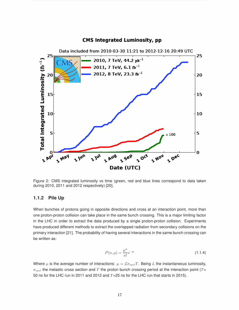
Figure 2: CMS integrated luminosity vs time (green, red and blue lines correspond to data takenduring 2010, 2011 and 2012 respectively) [20].
1.1.2 Pile Up
When bunches of protons going in opposite directions and cross at an interaction point, more than
one proton-proton collision can take place in the same bunch crossing. This is a major limiting factor
in the LHC in order to extract the data produced by a single proton-proton collision. Experiments
have produced different methods to extract the overlapped radiation from secondary collisions on the
primary interaction [21]. The probability of having several interactions in the same bunch crossing can
be written as:
P (n, µ) =µn
n!e−µ (1.1.4)
Where µ is the average number of interactions: µ = LσinelT . Being L the instantaneous luminosity,
σinel the inelastic cross section and T the proton bunch crossing period at the interaction point (T=
50 ns for the LHC run in 2011 and 2012 and T=25 ns for the LHC run that starts in 2015).
17
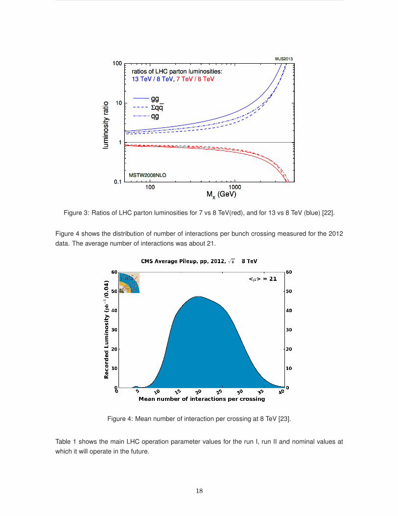
Figure 3: Ratios of LHC parton luminosities for 7 vs 8 TeV(red), and for 13 vs 8 TeV (blue) [22].
Figure 4 shows the distribution of number of interactions per bunch crossing measured for the 2012
data. The average number of interactions was about 21.
Figure 4: Mean number of interaction per crossing at 8 TeV [23].
Table 1 shows the main LHC operation parameter values for the run I, run II and nominal values at
which it will operate in the future.
18

Parameter Run I Run II (Expected) Nominal
Beam energy [TeV] 3.5 and 4 6.5 7
Max. delivered integrated luminosity (fb−1)6.1 (3.5TeV)
40-60 25023.3 (4TeV)
Bunch spacing [ns] 49.9 24.95 24.95
Full crossing angle [µrad] 290 298 590
Energy spread [×10−3] 0.1445 0.105 0.123
Number of bunches 1380 2508 2808
Injection energy [TeV] 0.450 0.450 0.450
Transverse emittance [×109π rad-m] 0.59 0.28 0.36
β∗, ampl. function at interaction point [m] 0.6 0.45 0.15
RF frequency [MHz] 400.8 400.8 400.8
Average bunch intensity [×1010 protons ] 16 12 22
Bunch length [cm] 9.4 9 9
Bunch radius [×10−6 m] 18.8 11.1 7.4
Peak Luminosity [×1033 cm−2s−1] 7.7 10-20 50
Table 1: Comparison between LHC parameters during Run I, Run II and nominal values [24].
19

Chapter 2
COMPACT MUON SOLENOID
EXPERIMENT (CMS)
CMS is a multipurpose detector designed to study the electroweak symmetry breaking mechanism,
and to search for signals of production of physics Beyond Standard Model (BSM) [12, 25]. The CMS
detector is installed at approximately 100 m underground near the French town of Cessy. It has a
total length of 21.6 m and a diameter of 14.6 m. The weight for the installation of all sub-detectors
and hardware related for readout and operation is about 12500 ton.
The main features of the CMS detector are:
• Compactness.
• A solenoid with a high magnetic field.
• A highly efficient muon detector system.
• A tracking system fully based on silicon detectors.
• Homogeneous system of PbW04 crystals in the electromagnetic calorimeter.
CMS consists of several sub-detectors (as shown in Figure 5), which are Tracker, Calorimeters (Elec-
tromagnetic and Hadronic) and Muon Chambers (Drift Tubes, Cathode Strip Chambers and Resistive
Plate Chambers).
One of the main elements of this detector is the magnet [12,25], which is a superconducting solenoid
that generates a magnetic field of 3.8 T, in its inner part, and 2 T in its return yoke. Superconducting
magnets are needed in order to generate a large magnetic field to bend the trajectory of high energy
charged particles, with the aim of measuring their momenta. The Tracking System and Calorimeters
are located inside the solenoid, while the Drift Tubes, the Cathode Strip Chambers and Resistive
Plate Chambers are outside. The Muon Chambers are intercalated with an iron structure that serves
20

Figure 5: CMS detector [18].
not only as support but also as a guide for the magnetic field. The magnet is 12.5 m long and 6 m of
diameter with a weight of 220 ton, and can store an energy of about 2.6 GJ.
Given the shape of the solenoid, CMS was designed to have one central barrel and two end-caps.
The experiment uses a right-handed Cartesian coordinate system with the origin at the center of the
detector (see Figure 6). The y-axis was defined pointing upward while the x-axis was defined pointing
towards the center of the LHC. In physical analyses, instead of using the polar angle (θ), the pseudo
rapidity (η) is more conveniently used, which is invariant under Lorentz boosts in the ’z’ direction and
it is defined as:
η = −ln(tan(θ2)) (2.0.1)
21

Figure 6: CMS coordinate system. Definition of pseudo rapidity (η) and azimuthal angle (φ) [18].
2.1 Sub-Detectors
2.1.1 Inner Tracking System
The Tracker System has a length of 5.8 m and a diameter of 2.5 m. It is the largest tracker ever built
with silicon and it is the first one using silicon detectors in the outer region of the tracker.
This sub detector can reconstruct the momentum of charged particles taking into account multiple
scattering and the energy loss in the material.
The tracker (Figure 7) is composed of the Pixel Detector which lies in the center of the detector and
the Silicon Strip Detectors (SSD) which surround it [12,25,26].
The working conditions of this sub-detector require a system designed to have a high granularity
and fast response, so that the trajectories can be identified and associated with the correct bunch
crossing. The density of hits per unit time and unit area within the tracker decrease with the radius.
22

Figure 7: Schematic of CMS Inner Tracking System [18].
For this reason, pixel detectors of 100×150 µm2 were chosen for radii below 20 cm, while, silicon
micro-strip detectors of 10 cm×80 µm and 25 cm×180 µm were selected for radii between 20 cm and
55 cm and radii between 55 cm and 116 cm, respectively. The CMS tracker has a total of 66 million
pixels and 9.3 million micro-strips.
The pixel detector is comprised of three cylindrical layers of 98 cm long in the barrel region at radii
of 4.4, 7.3 and 10.2 cm. Also there are two layers in the region of the endcap located at ±34.5 cm
and ±46.5 cm along the z-axis. Its acceptance covers a pseudo-rapidity region of |η|<2.5. The pixel
detector is crucial for the secondary vertex reconstruction, which is used for the b-jet identification
(see section 3.5).
The silicon micro-strip detectors are composed of three different subsystems. The internal tracker
within barrel and endcap (TIB-TID), the tracker in the outer region of barrel (TOB) and the external
tracker of endcap (TEC) .
The TIB is located in the radial region between 20 cm to 55 cm and has 4 layers. The first two
are double sided with sensors allowing a resolution in the z-axis of 230 µm. The resolution in the
transverse direction varies between 23 µm for the first two layers and 35 µm for the second two.
The TID is composed of three disks and also, the first two are double-sided. This subsystem is located
in the region from 80 cm to 90 cm in the z-axis. It covers |η|<2.5.
The TOB comprises six layers that are parallel to the z-axis. It has a length of 2.18 m and its sensors
are 500 µm thick. The resolution is 35 µm for the two outer layers and 53 µm for the first four. The
first two are double sided too.
Finally, TEC is located between 134 cm and 282 cm along the z-axis with a coverage of |η|<2.5. It
is composed on nine disks, each of them having 16 petals.
23

The pixel detector is the closest detector to the center of the beam pipe and for this reason, it is very
important for detecting short-lived particles.
SSD-Circuits are used to amplify signals and also to control information such as temperature and
time, so that tracks can be synchronized with collisions.
The transverse momentum resolution was measured using single muons. For values of pT between
1.0 and 10 GeV, a pT resolution less than 1% was found for |η|<1.9. A pT resolution of less than
2% was measured for other η ranges covered by the tracker. Also the momentum resolution was
measured for pT values of 100 GeV, a resolution better than 2% was found for |η|<1.6 and increasingly
degraded up to 7% for |η| values of 2.4.
2.1.2 Electromagnetic Calorimeter (ECAL)
The electromagnetic calorimeter (Figure 8) is used to measure the energy of electrons and photons.
This detector is made of crystals that scintillate when an electron or a photon passes through them,
due to the sudden gain and loss of energy of its electrons. The number of photons in each scintillation
is proportional to the energy of the particle that causes it.
Figure 8: Schematic of CMS ECAL. The values shown correspond to the η coverage [27].
The CMS electromagnetic calorimeter (ECAL) is a homogeneous and hermetic calorimeter made of
61200 crystals (PbWO4) in the barrel and 7324 crystals in each of the two endcaps [12,25,28]. High
density crystals are used in order to improve the response time, the granularity, and the radiation
hardness. PbWO4 has a high density (8.28 g/cm3) and a scintillation decay time of the same order of
magnitude that the time between bunch crossings (25 ns).
24
The ECAL, covers the region |η|<3 and has a thickness which is greater than 25 radiation lengths in
order to minimize the probability that a photon or an electron goes further out. ECAL crystals in the
barrel (EB) are segmented by ∆η ×∆φ=0.0174×0.0174 with a cross section of approximately 22×22
mm2. EB is read out with avalanche-photodiodes.
The ECAL in the endcap region (EE) covers a range of 1.48<|η|<3, where the crystals are grouped
in 5×5 segments (supercrystals) with a cross section of 30×30 mm2 and 28.62×28.62 mm2 for the
front and back side respectively. These are read out with vacuum-photo diodes because they are
more radiation resistant.
The ECAL contains a preshower detector which is located in front of the endcaps and has a finer
granularity. It is used to distinguish between π0 in jets from isolated photons, this is crucial in anal-
yses involving the process H → γγ. It is 20 cm thick and is composed of two layers of lead ab-
sorbers and silicon micro-strips, which are interleaved by two silicon detectors. It covers the region
1.653<|η|<2.6.
The energy resolution of the electromagnetic calorimeter can be modeled as:
(σ
E)2 = (
S√E)2 + (
N
E)2 + (C)2 (2.1.1)
Where, S is the stochastic term, N the noise and C the constant term. The values of these parameters
has been measured, for a 3×3 crystal matrix using test-beam data, to be: S=2.8%, N=12% and
C=0.3%.
2.1.3 Hadronic Calorimeter (HCAL)
The hadronic calorimeter (Figure 9) is used to measure the energy and direction of travel of hadrons
[12, 25, 29]. It is composed of several layers of absorbent material interleaved with layers of scin-
tillation material. When a particle enters the absorbent material, the interaction can produce many
secondary particles, these particles can generate more particles producing hadronic showers. When
these showers pass through the layers of scintillation material, they are activated and blue-violet light
is emitted. This light is shifted to the range of green wavelengths spectrum, and through optical fibers
it is sent into the readout box. Once there, the optical signals that come from sensors which are in
different layers (one after another, inside a geometrical region defined in the algorithms as towers) are
combined and used to determine the energy of the particles. After this, the resulting signals are am-
plified (2000 times) and converted into electronic signals by the use of hybrid photo-diodes (HPDS).
Then, the signals are sampled and digitized by integrated circuits (where charge integration and en-
coding is performed), and finally, the output of these circuits is sent as input to the data acquisition
system (DAQ) for purposes of Triggering and Reconstruction.
The HCAL is composed of brass absorbers and plastic scintillator layers. It is 11 interaction lengths
in depth.
25

Figure 9: Schematic of CMS HCAL [27].
The HCAL in the barrel (HB) is located between radii of 1.77 m and 2.95 m. It covers a region |η|<1.3
and has a granularity ∆φ×∆η=0.087×0.087.
HCAL in endcap (HE) is between 300 and 500 cm from the interaction point, along the z-axis and
covers a range 1.3<|η|<3. Its granularity is about ∆φ×∆η=0.035×0.08.
In addition, two forward hadronic calorimeter (HF) are placed in each CMS detector side, near the
beam axis (covering a region 3<|η|<5). Since the rates of hadrons in this region are very high, these
calorimeters were made up of quartz fibers and steel absorbers because they are more radiation-hard
materials.
There is another component called Outer Hadron Calorimeter (HO) which is outside the solenoid and
is used to detect the remnants of the highly energetic hadronic showers.
The energy resolution for hadrons of the combined calorimeter can be modelled as:
(σ
E)2 = (
S√E)2 + (C)2 (2.1.2)
Where, S is the stochastic term, N the noise and C the constant term. Table 2 shows the values
measured for the barrel and the HF.
26

Region S [%] C [%]
Barrel 84.7 7.4
HF 198 9
Table 2: HCAL energy resolution parameters.
2.1.4 Muon System
The muon system (Figure 10) has two main functions: identification of muons and triggering [12,25].
Figure 10: Schematic of CMS Muon Chambers [27].
The muon detectors are located in the outer part of the magnet because muons can penetrate several
meters of iron without interacting. Their coverage is |η|<1.2 and |η|<2.4 in the barrel and encap
region, respectively. Gas detectors are used because they have several advantages such as:
• A large radiation length.
• Can cover large volumes and/or areas.
27

• They are relatively inexpensive.
A Muon Chamber can be either a chamber with Drift Tubes (DT) and Resistive Plate Chambers
(RPC), or, a chamber with Cathode Strip Chambers (CSC) and RPCs. DTs and RPCs are arranged
in concentric cylinders around the beam path (the barrel region), while CSCs and RPCs, comprise
the endcaps.
The resolution for muons using only the muon system has been measured to be about 9% for pT ≤200
GeV and up to 15-40% for pT=1 TeV. The measurement was also performed combining the tracker
and the muon system information yielding a momentum resolution of 0.8-2% for pT ≤200 GeV and
5-10% at pT=1 TeV.
The upgrade performed during the long shutdown (the fourth layer has been completed for the outer
rings for both CSC and RPC systems) has enhanced the resolution by ∼2% for 1.2<|η|<1.8.
The Drift Tubes (DT):
The DTs are the traditional technology for low occupancy. For this reason, they are the muon detectors
used in the CMS barrel because a low rate and a relatively low magnetic field is expected in this
region [12,25].
The DTs are aluminum cells with only a few inches of thickness, which are filled with gas and have
an anode in the center. The anode collects the ionized charges that result when a charged particle
passes through the tube. These tubes are organized into three super-layers, each one composed of
four layers. Two of the super-layers are aligned parallel to the beam and the third one is perpendicular
to it. This geometry was defined with the aim of measuring the z-component. The coordinates are
detected in the following way: first, the place where the electrons collided with the anode is recorded,
then, the distance between the point of the muon trajectory and the anode is calculated. This distance
is given by the delay time multiplied by the speed of the gas’ electron shower.
The DTs cover a region of |η|<2.1 and have a position resolution of about 200 µm and a track
resolution around 1mrad along the φ direction. Figure 11 shows a schematic layout for one DT.
Figure 11: Schematic layout for one DT [30].
28

Cathode Strip Chambers (CSC)
CSCs are designed to operate in high magnetic fields and with neutron backgrounds up to 1 kHz/cm2.
They were chosen as the detectors to be used in CMS endcaps because in this region the rates of
muons and background levels are high and the magnetic field is large and non-uniform [12,25].
Each CSC consists of six gaseous layers that are in the radial direction acting as cathodes, which in
turn are crossed in a perpendicular way by anodes. When a muon passes through the chamber, it
ionizes the gas’ atoms, causing them to follow the path of the gaseous layer inducing a current over
the strips, it also makes that the released electrons follow the path of the anode. Thereby, with this
information it is possible to obtain the coordinates of the muon.
The CSCs identify muons between 0.9|η|<2.4 with a resolution of 200 µm (100 µm for ME1/1, which
is the region in the endcap that is the nearest to the collision point, see Figure 10) and an angular
resolution in φ of the order of 10 mrad.
Figure 12 shows a representation of a CSC with its wires and strips .
Figure 12: Representation of a CSC with its wires and strips [18].
Resistive Plate Chambers (RPC)
In CMS, the RPCs are located both in the endcap region (0.9≤|η|≤1.6) and the barrel region
(|η|<1.2) [12, 25, 31]. These are double-gap chambers, with a gap of 2 mm formed by two paral-
lel electrodes of bakelite with a resistivity of about 1010 Ω-cm. Each chamber has a readout plane
of copper strips between the two gaps. They are operated in avalanche mode to ensure smooth
operation at high rates. RPCs produce a quick response with good time resolution but with a spatial
resolution worse than that provided by DTs or CSCs. They can help to resolve ambiguities in the
case of multiple hits in a chamber. Each RPC consists of two parallel plates containing a gas inside
and connected to a potential difference around 9.2 kV. The gas is a mixture composed of: C2H2F4
(95.2%), C4H10 (4.5%) and SF6 (0.3%) with a humidity of 40% at 20-22 °C. When a muon passes
through the gas, it produces free electrons from gas’ atoms, which in turn produce other free electrons
and thus an avalanche is generated. This avalanche induces a current in the detecting external strips
which are used to locate the position of the muon.
29

In the barrel region there are 480 chambers with 68136 strips (with a width of 2.28 to 4.10 cm), which
covers an area of 2285 m2, while in the endcap region, 432 chambers are equipped with 41472 strips
(width of 1.95 to 3.63 cm) covering an area of 668 m2.
An RPC is capable of sensing an ionization event in a time about 1 ns. Therefore, a special muon
trigger device based on RPCs can identify the bunch crossing (BX) associated with a specific muon
track, even in the presence of the rate and background expected at LHC. The signals obtained from
these devices provide the time and position of the muon with the required accuracy.
Figure 13 shows a representation of an RPC with two gas gaps for one readout strip plane.
Figure 13: Representation of an RPC with two gas gaps for one readout strip plane [18].
Several high voltage scans were performed during 2011 and 2012 to study in detail the behavior of
all chambers and optimize operating points [31]. Collision data used for this study were registered for
various voltage points during dedicated runs.
The efficiency curve of each chamber partition was modeled using the sigmoid function:
ǫ(HV ) =ǫmax
1 + e−S(HV−HV50%)/ǫmax(2.1.3)
Where :
ǫ(HV ) : is the efficiency at the effective high voltage HVeff .
HV50%: effective high voltage at 50% of the maximum efficiency.
ǫmax: maximum efficiency (in plateau).
S : slope at HV50%.
HV : effective high voltage.
Examples of this curve can be seen in Figure 14.
30

Figure 14: Examples of the fit (blue curve) to the data taken (black points) during the second RPC-High Voltage Scan of 2012. The left (right) cross is the knee (working point) of the distribution. Theleft (right) plot corresponds to a chamber located in the endcap (barrel) region.
This study yielded efficiencies around 95% for each of the different chambers. Additionally, the agree-
ment between the efficiency measured in subsequent runs and the predicted using this adjustment
procedure confirmed the effectiveness of the technique. The software used for this procedure was
developed by the author of this thesis, as well as part of the code used to measure efficiency. Specifi-
cally, the code to measure the relative efficiency using global muons reconstructed without the use of
RPCs.
2.2 Data Management at CMS
2.2.1 Trigger And Data Acquisition System (DAQ)
The trigger system is used to filter the amount of information per unit of time that is generated in the
LHC collisions (O(107Hz)) to a range of O(102Hz) [12, 25, 32]. This filtering is needed in order to
be consistent with the electronic-readout capacity. Therefore, a reduction by a factor of about 105 is
necessary.
The architecture of the CMS Trigger System uses two levels of triggering: Level 1 (L1T) is performed
by electronic circuits designed specifically for the purpose of providing the first selection of collisions
with events with physics of interest to the experiment. These circuits are near the detector to avoid
loosing time in transmission of information. On the other hand, the High Level Trigger (HLT) is a set
of routines that run in commercial CPUs. These routines are in charge of selecting more complicated
objects than the L1 routines.
In the L1T, the time to process the information is limited by the storage capacity of the front-end elec-
tronics (FE), which can store information of up to 128 contiguous bunch crossings, which correspond
to a time of approximately 3.2 µs. During this time, information has to be sent from the FE to the
processing elements of the L1T, to make a decision and return it to the FE. The L1T uses coarse
information from the muon chambers and the calorimeters.
31

In the HLT, the rate should be reduced by a factor scale of 103 in order to be within limits allowed by the
data recording technology. About 1000 processors are used to achieve this end. These processors
are interconnected by a switched network. The HLT uses several algorithms to identify physics objects
(muons, electrons, photons, jets, etc.). In these algorithms, the selection criteria used are composed
of three modules:
1. Producer (partial reconstruction)
2. Filter (based on tables)
3. Prescaler (one out of N events is considered to be processed)
Finally, the output of the trigger should be such that:
• The background-rate is low.
• The efficiency of the signal is high.
• The time employed is low enough to avoid dead times.
The definitions of signal and background vary according to the physics objective of the trigger path.
2.2.2 CMSSW
CMSSW is the software used in the CMS experiment for reconstructing, filtering and analyzing the
data collected by the experiment [33]. This platform has been designed using a C++ framework. The
importance of this software is that it allows to work with information obtained by the detector (or by
simulation) in an easy and very organized way.
CMSSW is a platform designed to operate in a modular way in order to allow being developed and
maintained by a large group of geographically dispersed collaborators. Therefore, whenever a new
analysis or filter is developed, it can be added as a plug-in to the platform and also tools developed
by others can be used.
CMSSW is not only used to process data from the detector, but it is also used to process data obtained
by simulation (see chapter 4). The CMSSW version used for this analysis is CMSSW_6_2_11.
The core concept of CMS data model is the event. An event can be considered as an object in which
all the information coming from a collision is stored. The experiment stores, for each selected event,
all the reconstructed objects as well as the provenance information.
Events are physically stored in ROOT files. ROOT is a software that provides a set of object-oriented
tools with all the functionality needed to manage and analyze large amounts of data [34]. Among
its functionalities are: histograming methods, curve fitting, function evaluation, minimization, graphics
and visualization classes that allow to analyze data in an optimal way.
CMS data are classified as follows:
32

• FEVt (FullEVenT): all data collections of all producers, in addition to the RAW data. These are
useful for debugging.
• RECO (reconstructed data): contains selected objects from reconstruction modules.
• AOD (Analysis Object Data): a subset of the former containing only high-level objects. These
data are used in most analyses because their size is smaller.
2.2.3 GRID
The Worldwide LHC Computing Grid (WLCG) comprises four levels called Tier-0, Tier-1, Tier-2 and
Tier-3. Each level has a specific set of services [35].
Tier-0 is the CERN´s data center. This level is responsible for the safe keeping of the raw data and
carry out the first step in the reconstruction of the raw data into meaningful information (HLT). Due
to the large amount of data, the raw data and reconstructed outputs (both, real and simulated) are
distributed to Tier-1, which besides storing the data, performs reprocessing, distributes data to Tier-2
and stores part of the data that is produced at Tier-2. Tier-1 is connected via optical-fiber to Tier-0
(there are 13 computer centers belonging to Tier-1). Tier2 are computer clusters of universities and
other partner institutions that store data and allows researchers to use computer resources to run
analyses. There are about 155 Tier-2 sites worldwide. Tier-3 can be used by individuals to access
the network, however, there is no formal commitment between WLCG and Tier-3 resources.
To access the stored data and perform analysis on the Grid, different tools have been developed.
Among them is CRAB, which is the tool that was used for this analysis.
CRAB (CMS Remote Analysis Builder) is a tool written in Python that allows to run, in parallel, multiple
instances of CMSSW and, access information from different datasets (HLT results). CRAB also can
be used to run third-party software. For the present analysis CRAB was used to run MadWeight in
the GRID (see Appendix A).
33

Chapter 3
RECONSTRUCTION OF OBJECTS AT
CMS
The CMS collaboration has developed several algorithms to reconstruct objects from events. It also
has defined useful physics variables which are described below. Figure 15 shows a transverse slice
of the CMS detector as well as its interaction with different physical objects.
Figure 15: Particle detection.
34

MISS
3.1 Missing Transverse Energy (ETmiss)
Since the partons that compose a proton share their momentum, the initial longitudinal momentum in
a parton collision is unknown, however, the initial transverse momentum must be zero. For this rea-
son, ETmiss is a very important variable because neutrinos and hypothetical neutral weakly interacting
particles could escape the detector without leaving any trace, but, their presence can be inferred from
the imbalance of the total measured transverse momentum [36,37].
There are some cases in which ETmiss is not useful to conjecture the presence of particles that escape
detection because their contribution to the amount of ETmiss is zero, these cases are: events where
there are several particles escaping detection whose net transverse momentum is zero and events
with particles with momentum in the longitudinal direction that escape detection.
The Missing Transverse Momentum ( ~ETmiss) and the Missing Transverse Energy ETmiss are defined as:
~ETmiss: The imbalance of the event‘s total momentum in the plane perpendicular to the beam direction
( ~ETmiss = −∑ ~Pt)
ETmiss: The ~ETmiss magnitude.
CMS has developed three different algorithms to calculate the ETmiss.
Calorimeter ETmiss
In this case, ETmiss is calculated using exclusively the information obtained with the calorimeters. For
this purpose, the calorimeter is divided into towers which are the result of performing a segmentation
in the η − φ plane. The energy deposited in each tower is measured and if it is above the threshold
noise then it is included in the calculation of ETmiss. The threshold value is used to avoid including
some noise produced by the instruments. Table 3 shows the thresholds used for each region (see
sections 2.1.2 and 2.1.3).
Thresholds [GeV]
HB HO HE∑
EB∑
EE
0.9 1.1 1.4 0.2 0.45
Table 3: Thresholds used to form CaloTowers [38]. HB, HE and HO stands for HCAL in the barrel,endcap and outer region respectively, while EB (EE) stands for ECAL in the barrel (endcap) region.
Track-Corrected ETmiss
It is calculated by correcting the tower information mentioned before with the corresponding momen-
tum measured with the tracking system. Since the tracking system has an excellent linearity and
very good angular resolution, this correction is very useful to fix the imperfect calorimeter response to
charged hadrons.
35

Particle Flow ETmiss
Particle flow is a set of algorithms that are used in CMS to reconstruct all the objects using all the
information given by the sub-detectors. ETmiss obtained by particle flow is the most accurate because
information from all subsystems is used to determine the energy imbalance in the event. A more
detailed information can be found in section 3.7.
3.2 Photons and Electrons
When a high energy photon interacts with the detector material, an electron-positron pair is generated,
which in turn generates new photons because of Bremsstrahlung [25,39]. This process results in an
electromagnetic shower which is dispersed along the azimuthal angle (φ) due to the magnetic field.
To reconstruct photons at CMS, the crystals with a transverse energy greater than the energy of the
crystals that surround them, and above a predefined threshold are searched (seed crystals), then, for
each seed, a super cluster (SC) is generated with crystals in its neighborhood and, the total energy
deposited on them is determined. Thereafter, with the values of the energy deposited in each crystal
of the SC, the position of the particle is calculated.
In the barrel, the clusters have a fixed η-width of five crystals centered on the seed crystal and,
in the φ-direction, adjacent strips of five crystals are added if their total energy is higher than other
predefined threshold. If other clusters lie within an extended φ-window of +/- 17 crystals and are above
other threshold, they are also included in the SC. In the endcaps, fixed matrices of 5×5 matrices are
used.
The position of the particle is calculated as:
x =
∑
xiWi∑
Wi(3.2.1)
where Wi is the weight:
Wi =W0 + log(Ei
∑
Ej) (3.2.2)
and Ej is the energy of j-crystal.
The shower generated by a photon is similar to the shower generated by an electron. To distinguish
between them the inner tracker system is used. For electrons, the energy measured by the electro-
magnetic calorimeter and the momentum measured by the tracker must be similar.
To reconstruct electrons, two inner points are found through an extrapolation of the positions calcu-
lated by means of SCs (this extrapolation is carried out for positive and negative values of charge).
These points are used to find the associated tracks in the Silicon Tracker Detectors. This task is exe-
cuted by taking into account that fluctuations are not Gaussian because of Bremsstrahlung. For this
36

reason, the algorithms used in CMS are the Kalman Filter algorithm and the Gaussian Sum Filter [40].
Then, a pre-selection is performed according to the following criteria to ensure a correspondence be-
tween the ECAL super-cluster found and pixel detector hits:
• The energy-momentum matching between the super-cluster and the track must be: ERec/pin<3.
• |ηin| = |ηsc−ηtrack|<0.1, where ηsc is the super-cluster η position and ηtrack is the track pseudo-
rapidity at the closest position to the super-cluster position.
• |φin| = |φsc − φextrap.|<0.1, where φsc is the super-cluster φ position and φextrap. is the track φ
position at the closest position to the track super-cluster position.
• The ratio of energy deposited in the HCAL (H) tower that is just behind the cluster’s seed and
the energy of the Super Cluster (E) must be such that H/E<0.2.
Electron ID
Table 4 shows the criteria used to identify electrons using the the Medium Working Point.
Variable Barrel Endcap Description
pT >20 >20 Transverse momentum.
|φin| <0.06 <0.03 Azimuthal difference beween track and SC.
|ηin| <0.004 <0.007 Pseudorapidity difference between track and SC.
|σηη| <0.01 <0.03 Shower shape σ along η.
H/E <0.12 <0.1 Hadronic over electromagnetic energy.
d0 <0.02 <0.02 Transverse distance from PV.
dz <0.1 <0.1 Longitudinal distance from PV.
missing hits ≤1 ≤1
Table 4: Electron identification (ID) (Medium Working Point Requirements) [41].
3.3 Muons
Muon reconstruction is performed in three different ways [25,42]:
1. Standalone, Track reconstruction using only the muon system: This reconstruction combines the
information obtained by the DTs, CSCs and RPCs. The procedure used in this reconstruction
consists of an extrapolation (using a Kalman filter algorithm) of the information obtained from
the inner chambers, to predict the points in the outer chambers. Then, the predicted value is
replaced with the measured value. If there are not matching track segments or hits in a station,
the search continues for the next station. To make the propagation between stations, the Geant4
37

package is used, which takes into account the energy loss, multiple scattering and non-uniform
magnetic field. Finally, the Kalman Filter Algorithm is applied in reverse, from the outside and
the extrapolation is made to the nominal interaction point.
2. Global, this reconstruction uses a combined information obtained by the DTs, CSCs, RPCs and
the Inner Tracking System: In order to save resources, the process of reconstruction using the
Inner Tracking System is performed without using all the information recollected. It only uses
the region that has been predicted by the extrapolation mentioned in the standalone procedure.
3. Particle Flow : As was mentioned before, particle flow allows to reconstruct all the objects
(among them muons) using all the information given by the sub-detectors. A more detailed
information can be found in section 3.7.
Muon ID
Table 5 shows the criteria used to identify muons using the the Tight Working Point.
Variable Criterion Purpose
The candidate is a Global Muon
χ2/ndof of the global-muon track fit <10 To suppress hadronic punch-through
and muons from decays in flight.
Muon chamber hit included >0 To suppress hadronic punch-through
in the global-muon track fit and muons from decays in flight.
Number of matched stations >1 To suppress punch-through and
accidental track-to-segment matches.
IP of tracker track w.r.t. PV dxy<2 mm To suppress cosmic muons and further
suppress muons from decays in flight.
Longitudinal distance of dz<5 mm Loose cut to further suppress cosmic muons,
the tracker track w.r.t. PV muons from decays in flight and tracks from PU.
Number of pixel hits >0 To further suppress muons from decays in flight.
Cut on number of >5 To guarantee a good pT measurement
tracker layers with hits and suppress muons from decays in flight.
Table 5: Muon identification (ID) (Tight Working Point Requirements) [43].
3.4 Jets
The algorithms to find jets can be classified into two categories which are: the recombination and the
cone algorithms [44,45].
38

Recombination Algorithms
In this kind of algorithms the two closest particles (according to the metric di,j , see below) are merged
into one particle that is the result of the addition of their four-vectors. Then, this process is re-
peated several times until the distance of separation is higher than a predefined value (dmin , typically
dmin =0.5). The distance can be defined in several ways, therefore, different algorithms have been
implemented. The most common definitions use the expressions:
dij = min(P 2nti , P
2ntj )
Ri,jd2min
(3.4.1)
∆Ri,j =√
(ηi − ηj)2 + (φi − φj)2 (3.4.2)
Where:
Ptk : is the transverse momentum of the k-th particle.
(ηi, φi): is the direction of the i-th particle.
And n is a parameter that defines the algorithm. Typical values are shown in Table 6 [44,45].
n Algorithm
0 Cambridge/Aachen
1 kt
-1 Anti-kt
Table 6: n-value for some recombination algoritms.
Cone Algorithms
In this type of algorithms the process starts with a set of particles used as seeds, which are chosen
arbitrarily. For each of these seeds, a cone is constructed to have certain predefined radius (R,
typically R =0.5) and, the same direction as the momentum of the particle used as seed (ηs, φs).
Then, the particles inside the cone are found using the criteria:
∆Ri,s =√
(ηi − ηs)2 + (φi − φs)2 < R (3.4.3)
Where:
(ηi, φi): is the direction of the i-th particle.
After this, the net momentum of all particles inside the cone is calculated and, a new cone is defined
with the same radius and pointing in the same direction as the net momentum obtained. This process
is repeated until it results in stable jets.
39
Since the set of seeds is chosen arbitrarily, it can happen that some resulting cones are overlapped.
One solution is to execute a process of splitting or merging cones depending on their overlapping
percentage. Another solution is to construct the jet associated with the particle with the highest
momentum and then, remove all the particles inside the resulting cone and repeat the process with
the remaining particles.
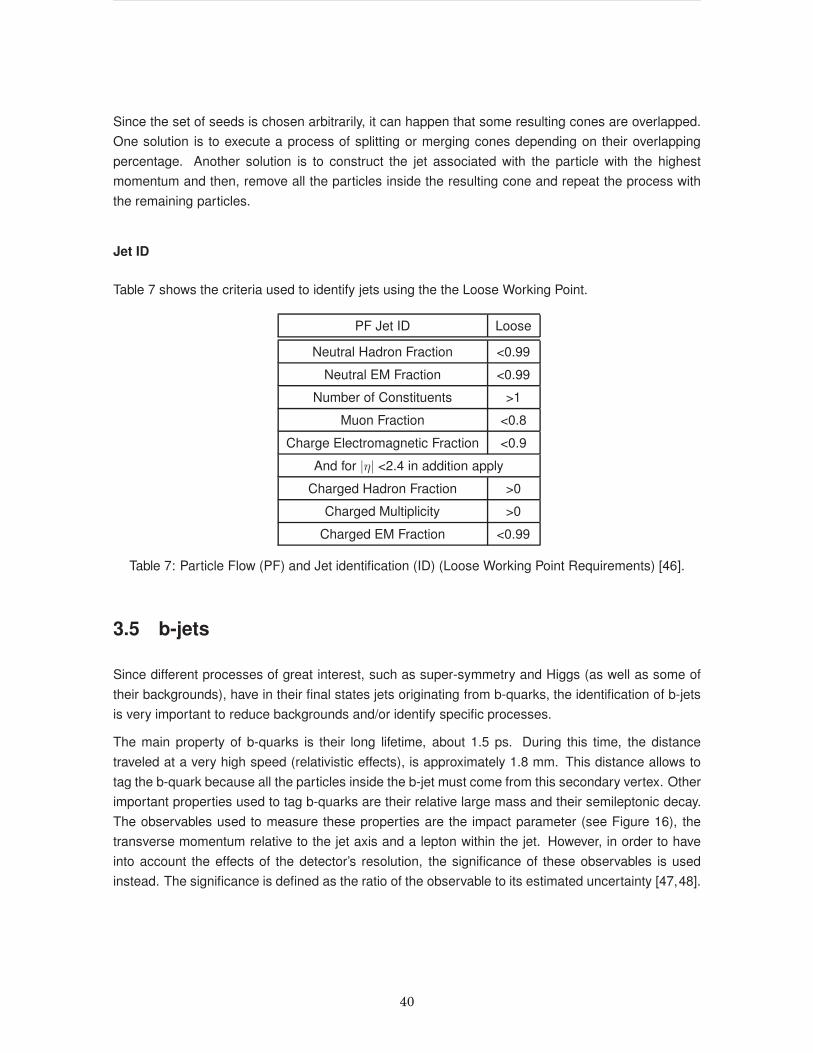
Jet ID
Table 7 shows the criteria used to identify jets using the the Loose Working Point.
PF Jet ID Loose
Neutral Hadron Fraction <0.99
Neutral EM Fraction <0.99
Number of Constituents >1
Muon Fraction <0.8
Charge Electromagnetic Fraction <0.9
And for |η| <2.4 in addition apply
Charged Hadron Fraction >0
Charged Multiplicity >0
Charged EM Fraction <0.99
Table 7: Particle Flow (PF) and Jet identification (ID) (Loose Working Point Requirements) [46].
3.5 b-jets
Since different processes of great interest, such as super-symmetry and Higgs (as well as some of
their backgrounds), have in their final states jets originating from b-quarks, the identification of b-jets
is very important to reduce backgrounds and/or identify specific processes.
The main property of b-quarks is their long lifetime, about 1.5 ps. During this time, the distance
traveled at a very high speed (relativistic effects), is approximately 1.8 mm. This distance allows to
tag the b-quark because all the particles inside the b-jet must come from this secondary vertex. Other
important properties used to tag b-quarks are their relative large mass and their semileptonic decay.
The observables used to measure these properties are the impact parameter (see Figure 16), the
transverse momentum relative to the jet axis and a lepton within the jet. However, in order to have
into account the effects of the detector’s resolution, the significance of these observables is used
instead. The significance is defined as the ratio of the observable to its estimated uncertainty [47,48].
40
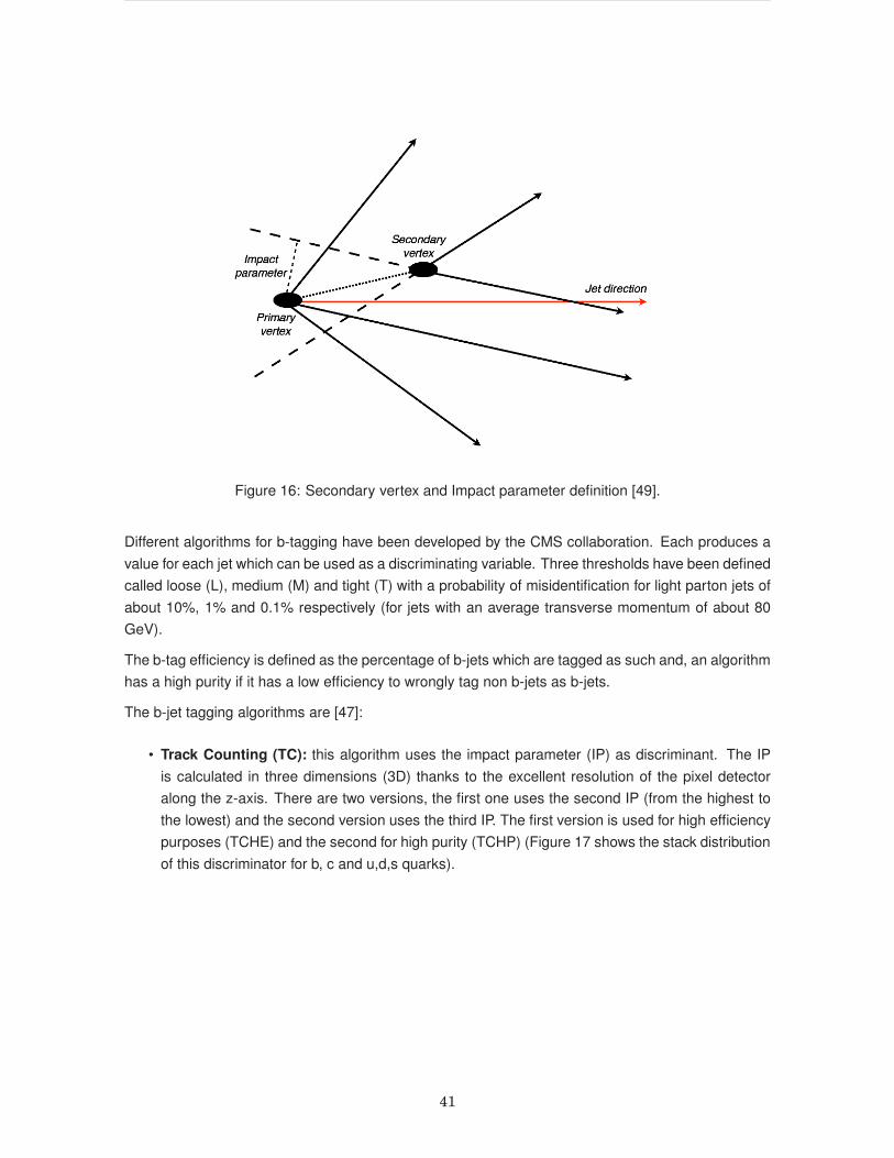
Figure 16: Secondary vertex and Impact parameter definition [49].
Different algorithms for b-tagging have been developed by the CMS collaboration. Each produces a
value for each jet which can be used as a discriminating variable. Three thresholds have been defined
called loose (L), medium (M) and tight (T) with a probability of misidentification for light parton jets of
about 10%, 1% and 0.1% respectively (for jets with an average transverse momentum of about 80
GeV).
The b-tag efficiency is defined as the percentage of b-jets which are tagged as such and, an algorithm
has a high purity if it has a low efficiency to wrongly tag non b-jets as b-jets.
The b-jet tagging algorithms are [47]:
• Track Counting (TC): this algorithm uses the impact parameter (IP) as discriminant. The IP
is calculated in three dimensions (3D) thanks to the excellent resolution of the pixel detector
along the z-axis. There are two versions, the first one uses the second IP (from the highest to
the lowest) and the second version uses the third IP. The first version is used for high efficiency
purposes (TCHE) and the second for high purity (TCHP) (Figure 17 shows the stack distribution
of this discriminator for b, c and u,d,s quarks).
41

Figure 17: 3d IP significance distribution [47].
• Jet Probability (JP): this algorithm computes the likelihood that all tracks associated with the
jet are coming from the primary vertex. This likelihood is the variable used for discriminating.
There is a modified version called JetB that gives greater weight to the tracks with the highest
IPs (Figure 18 shows the stack distribution of this discriminator for b, c and u,d,s quarks).
• Simple Secondary Vertex (SV): the variable used by this algorithm as discriminator is the flight
distance significance. As the TC algorithm it has two versions, the first one uses the second
highest flight distance and the second version uses the the third with the highest value. Again,
the first version is used for high efficiency (SVHE) and the second for high purity (SVHP) (Figure
19 the stack distribution of this discriminator for b,c,u,d,s quarks is shown).
42

Figure 18: JP discriminator distribution [47].
Figure 19: 3D SV flight distance significance distribution [47].
43

• Combined Secondary Vertex (CSV): this is a complex algorithm that additionally uses the
lifetime information obtained from tracks. This method is the most robust and provides discrimi-
nation even when there are not secondary vertexes reconstructed (the stack distribution of this
discriminator for b, c,u,d,s quarks is shown in Figure 20).
Figure 20: CSV discriminator distribution [47].
Since it is difficult to model all the parameters used to identify b-jets, the measurement of the perfor-
mance has to be obtained by a direct comparison to data. To this end, different methods have been
developed in CMS, which can be classified into two groups:
• Measuring efficiency using events from top quark decays: This method is used because
the branching ratio for the decay of the top quark to one W boson and one b-quark is very high
(99.8%). Therefore, a branching ratio (BR) of 100% is assumed and, the efficiency is measured
as the ratio between the number of b-tagged jets and the number of events.
• Measuring efficiency by using events with a soft muon within a jet: Since the b-quark
mass is relatively high, the muon momentum component that is transverse to the jet axis (pTrel)
is greater for muons from b-hadrons than for muons from charm hadrons. Furthermore, the
impact parameter (IP) of the muon track, calculated in three dimensions, is also higher for b-
hadrons. For these reasons, both of these variables can be used as discriminants in determining
44

the efficiency of b-tagging. In both cases, the discriminating power of the variable depends on
the muon jet pT , being pTrel(IP) better for jets with pT lower (higher) than about 120 GeV.
Figure 21 shows the efficiencies measured by the CSV algorithm.
Figure 21: CSV efficiency: The arrows (right to left) show the tight, medium and loose thresholds. SFis the ratio between data and simulated events [47].
3.6 Top Quarks
The top quark is the most massive particle known today, its mass is about 173 GeV. The top quark
has a very small lifetime, it almost immediately decays into b-quarks and W-bosons, which in turn
decay into others. The decays of the W bosons are the key in the t-quark reconstruction process.
At the LHC (with a center of mass energy of 8 TeV) top quarks [50] are mainly produced by:
• Gluon-gluon fusion: production of top quark pairs with a cross section of 245.8+6.2+6.2−8.4−6.4 pb.
• Drell-Yan/gluon fusion with a W boson: Single top production with a cross section of 87.1+0.24−0.24 pb
where 65% and 35% are the relative proportions of t and t respectively (t-channel). And a cross
section of 5.5+0.2−0.2 pb where 69% and 31% are the relative proportions of t and t respectively
(s-channel).
45

Given that a top quark decays mainly to a W boson and a b quark. The different decays of the W
boson define the final topology of the event. In the case of top quark pairs, three main signatures are
defined:
• Full hadronic (BR=45.7%), where both W boson decay hadronically.
• Full leptonic (BR=10.5%), where both W bosons decay leptonically (W → ℓν).
• Semileptonic (BR=43.8%), where one W boson decays to hadrons and the other to a lepton and
a neutrino.
tt topologies are similar to SUSY: Jets, MET and eventually leptons. They represent the control
sample for many analysis trying to discover SUSY.
3.7 Particle Flow (PF)
The CMS collaboration developed a technique known as particle flow (PF) which reconstructs and
identifies all stable particles in the event making use of the information collected by all CMS sub-
detectors [51]. All sub-detector information is combined into PF candidates which are: charged
hadrons, neutral hadrons, electrons, photons and muons.
The process to reconstruct objects is as follows: first, the net transverse momentum associated with
each vertex is calculated and the vertex with the highest value is selected as primary vertex (PV).
Then, electrons are identified and tracks and clusters used in this task are not used for identifying
other objects. After that, muons are identified and their tracks are no used for further identification
of other candidates. Next, the remaining tracks are extrapolated through the calorimeters and if they
fall within the limits of one or more clusters, the clusters are associated to the track. The resulting
set of track-cluster(s) is identified as a charged hadron and this set is not used for other identification.
Once all tracks have been used, the remaining clusters give rise to photons (ECAL) and neutral
hadrons (HCAL). Then, the resulting particles (electrons, muons, charged hadrons, photons and
neutral hadrons) are used to reconstruct the jets, the missing transverse energy and, to reconstruct
and identify the tau decays from their products and also, to measure the isolation of the different
particles.
3.8 Selection and Corrections Applied to Objects at CMS
3.8.1 Jets
The purpose of the jet energy calibration is to match the energy of the jet measured by the detector
and the energy of the corresponding true particle jet. A true particle jet is the jet resulting from the
clustering (same clustering algorithm applied to the jets of the detector) of all stable particles from
46

parton fragmentation and underlying event activity (UE). A correction is applied as a multiplicative
factor C for each component (µ) of the raw jet four-momentum as:
pcorµ = C × prawµ (3.8.1)
The correction factorC is composed of the offset correction (Coffset), the MC-calibration factor (CMC ),
and residual corrections for the relative (Crel) and absolute (Cabs) energy scales [52]. The first cor-
rection level, subtracts the additional energy generated by pile up effects. The second, corrects
reconstructed jets to compensate the nonlinear response of the calorimeter as function of pT and
variations in the response as function of η. These corrections are derived from simulation. And the
third, applies small residual corrections based on measurements of the relative scale, as function of η
(based on dijet events (Crel)) and, of the absolute scale, in the central region of the detector (|η| <1.3)
for Z + jets and γ + jets events (Cabs). Therefore, this correction is summarized as:
C = Coffset(prawT )× CMC(p
offsetT )× Crel(η) × Cabs(p
allT ) (3.8.2)
where poffsetT is the transverse momentum of the jet after applying the offset correction and pallT is the
pT jet after all the above corrections.
L1 - Pileup corrections
This correction makes use of two variables which are the jet area (Aj) and the pT density (ρ). Aj , is
defined as the region in φ − y space of each jet, occupied by soft particles that are artificially added
to the event (soft enough to not affect the real jets) and that are used in the reconstruction of jets [52].
And ρ, is defined for each event as the median of the distribution of pT per unit area, pTj/Aj , where
j runs over all the jets in the event. These variables are used to calculate the effect of the additional
particles and thus to calculate the correction factor to be applied.
L2L3- MC Corrections
The L2L3 corrections are based on simulation and correct the energy of the jets reconstructed so
that it is equal to the average energy of the jets at particle level. For this purpose, simulated jets
events, generated with PYTHIA6, tune Z2 and processed with full detector simulation (GEANT4) (see
chapter 4), are used in the derivation of these corrections. The jets so generated are matched with
the reconstructed according to the criterion: ∆R =√
(φ)2 + (η)2<0.25 to determine the response
precoT /pgenT for fine bins of pgenT and ηgen. With this information, the correction factor is determined as
the inverse of the mean response as a function of precoT for fine η-bins [52].
47

Relative Scale Correction
This correction factor is calculated using Z + jet events selected from collision data and assuming the
conservation of energy in the transverse plane [52]. This allows comparing the pT of the reconstructed
jet with the transverse momentum of the photon or the Z boson produced. The advantage thus
obtained is a better energy resolution because photon reconstruction is based only on information
from ECAL (see section 2.1.2).
Absolute Scale Correction
To find this factor correction, QCD dijet events for which one of the reconstructed jets is in the control
region (|η|<1.3) and other is outside, are used [52]. Since the pT of the two jets must be the same,
any difference between them translates into a calibration factor to be applied on the pT of the reco-jet
outside the control area. This correction makes the response flat as a function of η.
3.8.2 Missing Transverse Energy
Although ETmiss distribution should be independent of φ, the reconstructed ETmiss is dependent of φ
as an sine function (approximately). The causes of this anisotropic behavior can be inactive cells
and detector misalignment, among others. It has been found that the modulation amplitude increases
more or less linearly with the number of pile-up interactions.
Additionally, there are some anomalous ETmiss among them are [53,54]:
1. Secondary particles produced from the interaction of the particle beam with the residual gas
inside the LHC or particles produced outside the cavern (mainly muons). This type of noise
is called "beam halo". This type of fake MET can be reduced with the combination of the
timing information from the trigger system and the CSC detectors (> 90%) without rejecting a
considerable amount of good physical events (<0.5%) .
2. Malfunction of a component of the detector or event reconstruction. Such as:
• Hard collisions position displaced from the nominal point of interaction. Such events are
rejected efficiently by using the transverse momentum of tracks originating from the primary
vertex and the total hadronic event activity.
• The Tracker silicon strip may be affected by coherent noise. It is greatly reduced by the L1
trigger.
• Individual crystals in ECAL other than those already identified as dead crystals (crystals
that have been detected as noisy and are not used in the reconstruction) sometimes pro-
duce pulses of high amplitude due to an instrumental error. The rejection of these events
is done by comparing the energy deposits in crystals surrounding these crystals.
48

• Abnormal noise sources has been identified as noise above the expected electronic-noise
in the HCAL. This noise may be due to the hybrid-photodiods (HPDS) or the reading
boxes (RBX). Rejection of such events is based on comparing the measured total elec-
trical charge in a RBX for different time intervals and the difference between shapes of
noisy and nominal pulses.
• HCAL misfire laser system.
For these reasons, CMS has developed a set of clean up filters to reduce the amount of fake ETmiss.
Table 8 shows a list of the most important of them.
Clean Up Filters
≥1 Primary Vertex
Beam scraping events
HBHE noise filters
CSC beam halo filters
Tracking failure filter
ECAL/HCAL laser events
EE bad super crystal filter
ECAL dead cell trigger primitive filter
ECAL laser correction filter
Table 8: Clean Up Filters for ETmiss.
ETmissperformance at CMS has been studied in three different channels: Z → µµ, Z → ee and γ +
jets.
A strong agreement between observed data and simulation has been found in all of them.
3.8.3 Leptons
Isolation
The isolation is based on the PF approach as defined in [55]. There are two types of isolation. The
first is the relative isolation, which requires that the relative amount of PF transverse momentum with
respect to lepton transverse momentum in a cone centered around the lepton trajectory with ∆R<0.5,
is lower than 0.15:
Iso =
∑
pchargedHadT +∑
pneutralHadT +∑
pγTpℓT
< 0.15 (3.8.3)
Where:
49

pℓT is the lepton transverse momentum.
pchargedHadT is the transverse momentum of charged hadrons.
pneutralHadT is the transverse momentum of neutral hadrons.
pγT is the transverse momentum of photons.
and the sums are performed over all the PF candidates within the cone explained above. Figure 22
shows a sketch of the isolation criterion.
Figure 22: Sketch of lepton isolation.
The second, is the absolute isolation, this isolation demands that the scalar sum of the pT , of all PF
particles excluding the lepton itself, is lower than 5 GeV within a cone about the lepton trajectory with
∆R<0.5.
Pile-up Correction
Electron identification is based on the relative isolation of candidate electrons. This isolation process
is very sensitive to additional deposits of energy caused by pile-up resulting in an over-rejection of
candidates, thus, reducing the efficiency of identification [55]. Therefore, an algorithm similar to that
described in section 3.8.1 is used, where the effective area (Aeff ) is defined as the geometric area of
the isolation cone, reduced by a factor to account for the dependence respect to the pseudo-rapidity.
The effective area is determined in samples of Z → ee for specific periods of data taking. The ρ
50

parameter is also used and it is defined as the median of the distribution of the energy density of the
particles within the jet area in any event. The correction is then written as:
Iso =
∑
pchargedHadT +max(0,∑
pneutralHadT +∑
(pγT − ρAeff ))
pℓT(3.8.4)
The isolation of the muon is also corrected to take into account the effects of pile up. To this end, the
candidates are divided into two groups: associated and not associated with the primary vertex [55].
The charged particle candidates not associated with PV can be used as an estimate of the contribution
to pile-up of neutral particles candidates. For this purpose, it is defined the variable β as the ratio
between charged and neutral hadron production, which has been found to be β ≈2 (in average).
Thus, the resulting muon isolation can be written as:
Iso =
∑
pchargedHadT +max(0,∑
pneutralHadT +∑
pγT − 1β
∑
pcharged,NPVT )
pℓT(3.8.5)
The efficiency in the identification and isolation of leptons has been measured in Z → ℓℓ events. The
values thus obtained are: 91% for muons and 84% for electrons with small variations that depend on
the value of pT and η.
3.9 Systematic Uncertainties
3.9.1 Luminosity
The luminosity is measured using the forward hadronic calorimeter (HF) and the pixel detector. With
the calorimeter it is possible to perform a measurement in real time while the measurement with the
pixel detector must be done off-line due to the stable beam conditions required. The HF measurement
has a statistical error lower than 1% and can be performed in less than 1 s. On the other hand, given
the low occupancy, the measurement with the pixel detector has very good stability over time [56].
Pixel cluster counting method
This method is used to measure the luminosity based on the average amount of pixel clusters that
occur in an event with zero bias (only two bunches cross at the interaction point). The instantaneous
luminosity is related with the number of collision per crossing µ by:
νµ = LσT (3.9.1)
with ν being the frequency of the beam revolution and σT the total inelastic cross section.
51

Thus, luminosity can be calculated in terms of the average number of clusters per event (〈n〉 = µn1
with n1 being the average number of clusters per inelastic collision) and the visible cross section
(σvis = σT n1) as:
L =ν 〈n〉σvis
(3.9.2)
The visible cross-section is calibrated through Van der Meer (VdM) scans, which are a technique to
determine the beam overlap based on the shape of the measured rates as a function of the beam
separation. To this end, beams are scanned along the horizontal and vertical planes.
The minimum time interval to be considered in estimating the luminosity is the luminosity section (LS),
defined as 218 orbits, which corresponds to a time of 23.31 s. The instantaneous luminosity for each
LS is calculated using the number of clusters per event and with this value, the integrated luminosity
is calculated as the sum of the luminosities of each LS recorded by CMS and considered good for
physical analysis.
The main causes of uncertainty in this measurement are described in Table 9.
Source Description (Effects due to ...) Uncertainty (%)
Dynamic β∗ different values of β∗ 0.5
Beam-beam electromagnetic forces between the beams 0.5
Orbit drift 0.1
Emittance growth the increase of beam emittance 0.2
Lenght scale the nominal beam separation 0.5
Ghost and satellites spurious charges 0.2
Beam current calibration 0.3
Fit model 2
Afterglow Out-of-time response from mild activation 0.5
Dynamic inefficiencies Very high rate (can fill the read-out buffers) 0.5
Stability versus pileup 1
Stability versus pileup 1
Table 9: Sources of Luminosity Uncertainties.
3.9.2 Trigger and Lepton ID Efficiency
The efficiency in identifying leptons and lepton triggers is measured using a Tag & Probe method
(usually, on Drell-Yan di-eletron or di-muon events) which is used for data and simulation, as well as
for determining the scale factors. Lepton tag must pass all the requirements of selection of electrons
or muons. While the probe lepton is selected based on more flexible requirements that depend on the
efficiency measured. There are a number of variations of the tag and probe method. The simplest
52

variant is the counting tag and probe where efficiency is measured as the percentage of events that
pass the tag and probe method [57].
The experimental systematic uncertainties associated with leptons arise primarily from efficiency
measures, scale and energy resolution, and estimation of the background misidentified lepton yields.
The impact of this uncertainties is usually estimated by applying scale factors (event by event) in
predictions of efficiency (from simulation).
3.9.3 Jet Energy Scale
Each of the corrections applied to jets have uncertainties arising from sources such as:
• MC physical modelling of showers, underlying events, etc.
• Modeling of the detector response.
• Possible bias in the methodologies used to calculate corrections.
Several of these sources of uncertainty are related and can be combined into groups such as: ab-
solute scale, relative scale, pT extrapolation, pile-up, jet flavor and time stability. In CMS the total
uncertainty in the energy jet correction is calculated as the addition of each individual uncertainty in
quadrature.
The measurement of any physical quantity related with jets must include the uncertainty estimation
due to the uncertainty in the jet energy calibration. The most common practice is the evaluation of
the change in the measured quantity when the jet energy is fluctuated up and down according to the
total uncertainty of jet energy [58].
3.9.4 b-tagging
The principal cause of systematic uncertainties in b-tagging are the probability of misidentification
of a light parton jet and, secondary interactions of charged particles in the detector material. The
impact of these uncertainties on an specific analysis is calculated as follows: the scale factors found
in studies of efficiency (see section 3.5) are applied to the efficiencies associated with the working
point and new cuts of discrimination are calculated (each scale factor is applied in accordance with
the jet flavor). Then, efficiencies and rates of mistag associated with these new values are shifted up
and down by their associated uncertainties to find new b-tag cuts. Finally, the results of the analysis
under study obtained with the original cuts and with the new cuts are compared and the systematic
uncertainty can be obtained as the relative error between these results [47,48].
53

Chapter 4
EVENT SIMULATION
In HEP, use of simulations is essential to develop analyses that allow discriminating between events
coming from the process under study and, events resulting from its associated background processes.
These simulations should be as accurate as possible with respect to the data obtained experimentally
(or possibly obtained in case of theoretical predictions). Additionally, there should be a large number
of simulated events, so that the obtained distributions are representative of the process involved,
having high statistical accuracy.
Simulations must include:
1. MC Event Generator.
2. Simulation of the hadronization that is caused by the interaction of partons.
3. Effects caused by the detector’s resolution.
The techniques used to accomplish these tasks are based mainly on two methods: Matrix Elements
(ME) and Parton Showers (PS), which are described in section 4.1. In section 4.2, a brief description
of the software used in this analysis to implement these techniques is given and, in section 4.3, the
corrections due to luminosity and PU, that must be applied to simulated events in order to match real
data, are explained.
4.1 Matrix Elements and Parton Showers
The matrix elements method provides the likelihood that a certain event has been produced from
a specific process [59, 60]. It is obtained by calculating the amplitudes involved in the Feynman
diagrams for the process studied. It can be used with MC techniques to create numerous events,
each with the four vector for every object in the final state. For proton-proton collisions, the cross
section of the hard-scattering is:
54

dσp(a1a2 → x) =
ˆ
y
∑
i,j
(2π)4|Mp(a1a2 → y)|2fi(a1, Q2)fj(a2, Q2)
ε1ε2sdΦnf
(4.1.1)
Where:
a1a2: kinematic variables of the partonic initial state.
x: kinematic variables of the partonic final state.
Mp: matrix element of the process.
s: center of mass energy squared of the collider.
ε1ε2: momentum fractions of the colliding partons.
dΦnf: element of nf -body phase space.
fk(al, Q2): parton density function (PDF).
The PDF (fk(al, Q2)) gives the probability of finding a parton of flavour k, within the proton, carrying
a fraction al of the proton’s energy at an energy scale Q2 of the interaction [59]. The PDF can not be
calculated perturbatively because of the asymptotic freedom of QCD. However, its evolution can be
described due to its scale-dependence.
The evolution is performed by the parton shower (PS) and must be calculated from the initial scale
Q2 to a new scale in which the initial parton branches into two daughter partons. This process have
to be repeated with the new daughter particles until the lower cut-off scale is reached. Sudakov form
factors are used to perform this evolution. They give information related with the probability that a
branching occurs.
ME and PS are also used to take into account remnant partons, ie, in the collision, the interacting
partons are not only those involved in the hard-scattering but also the partons that interact softly.
Therefore, a correction to the evolution has to be considered. These corrections are known as under-
lying event and also serve to consider multiple interactions (PU).
In this analysis, the method of matrix elements is not only used to generate simulated events but also
as a tool for discriminating between signal events and background events (see section 7.4.3).
4.2 Tools for HEP-Simulation
There are different tools to perform the above tasks. In this analysis, the preselected samples used
(see section 7.1) were generated using MadGraph, Pythia, POWHEG, Geant4 and FASTSIM.
MadGraph5 is a tool based on the method of matrix elements that allows the generation of events
for any model that can be written in a Lagrangian form [61]. It makes next to leading order (NLO)
computations. This tool is written in Python and can be interfaced with other tools such as Pythia.
Pythia 8.2 is a tool for generating events in high-energy collisions. It can perform all the different
tasks listed above [62]. However, in the generation of the preselection samples used in this analysis,
55

Pythia was only used for simulating the parton showers. MadGraph and Pythia can be used together
because both of them use the standard formats given by the Agreement of Les Houches (LHA) and
the associated files Les Houches Event Files (LHEF). For the simulation of parton showers, the matrix
elements method is used to simulate the strong interaction between partons, which is the responsible
for the creation of new quark-antiquark pairs. Since this process is repetitive, Pythia must simulate
the evolution until a new scale in order to get good agreement with experimental data.
POWHEG program is an improvement of Pythia because it uses NLO calculations together with PS.
The main idea of the method is that the hardest emission is simulated according to the exact NLO
cross section, and this emission is excluded during the PS. In addition, all the subsequent emissions,
that are harder than this, are vetoed. This method provides a better description of the processes and
is used to simulate low-multiplicity final states.
Geant4 (Geometry and tracking) is a tool to simulate the interaction between the resulting particles
after collision (and hadronization) and the material of the different detectors used. It was originally
developed at CERN and now is maintained and developed by the Geant 4 Collaboration [63].
Finally, FASTSIM is a tool to perform a fast simulation of the CMS detector. It is an object-oriented tool
and is included in the CMSSW platform (see section 2.2.2). It is an alternative and a complementary
tool to Geant4 (commonly called as full simulation), with respect to which it is validated and tuned
regularly.
We describe in detail the MC used for background and signal in sections 7.1.2 and 7.1.3, respectively.
4.3 MC Corrections
As mentioned above, the CMSSW platform allows to use RAW data and simulated events in the
same way, which is very convenient as it allows to perform tasks such as triggering, reconstruction
and corrections using the same scheme. Additionally, the simulated events must be normalized to
luminosity to obtain consistency with the observed data. This normalization is obtained by multiplying
each event by a weight that can be obtained as follows:
Wi =σiL
ni(4.3.1)
Where:
Wi: weight applied to the i-th event.
σi: cross section of the process of the i-th event.
L: integrated luminosity.
ni: number of simulated events of the same process as the i-th event.
The MC samples are also corrected to match the true distribution of pile up in data. To this purpose,
pile up events are simulated using a minimum sample bias, where, for each event, the number of
56

pile up events is chosen randomly from a Poisson distribution with a mean that is over the allowed
range of expected pile up. This distribution is previously re-weighted to match the measured CMS
instantaneous luminosity. This set of weights is known as a "scenario".
57

Chapter 5
STANDARD MODEL (SM)
The standard model is a physical theory developed to unify the weak and electromagnetic forces [1–4].
This theory uses three concepts which are: the group of symmetries, the local gauge invariance and
the spontaneous symmetry breaking. According to the SM, the particles that make up matter are
representations of the group of symmetries SU(3)C×SU(2)L×U(1)Y . These particles are fermions
and there are three generations of them. These particles have a semi-integer spin. The principle of
local gauge invariance is the responsible for the force carrier particles (bosons). Applying this principle
on the groups SU(3)C and SU(2)L×U(1)Y produces the bosons of the strong and the electro-weak
forces, respectively. The principle of spontaneous symmetry breaking (SSB) is the responsible for
the mass of all the elementary particles. This principle states that there is a field that interacts with
particles (called Higgs field), and as result of this interaction the particles acquire mass. The gauge
boson of this new field is called the Higgs boson and is one of the predictions of the SM that has
recently been verified at the LHC by the ATLAS and CMS experiments [64].
Table 10 (Table 11) shows the main properties of the elementary fermions (bosons) of the SM.
The sector that defines the interactions between quarks and gluons is called Quantum Chromody-
namics (QCD). The Lagrangian of this sector is:
LQCD =i U (∂µ − igsGaµT
a)γµU + iD (∂µ − igsGaµT
a)γµD (5.0.1)
Where:
Gaµ :SU(3) gauge field.
T a : SU(3) generator.
γµ : Dirac matrices.
D and U : Dirac spinors associated with up and down type quarks.
gs : Coupling constant.
58

Name Symbol Generation Mass [MeV] Charge
electron e I 0.51 -1
electron neutrino νe I <2×10⁻⁶ 0
muon µ II 105.66 -1
muon neutrino νµ II <2×10⁻⁶ 0
tau τ III 1776.82 -1
tau neutrino ντ III <2×10⁻⁶ 0
up quark u I 2.3 2/3
down quark d I 4.8 -1/3
charm quark c II 1275 2/3
strange quark s II 95 -1/3
top quark t III 173.5×10³ 2/3
bottom quark b II 4180 -1/3
Table 10: Elementary fermions of the SM.
Name Symbol Mass [GeV] Charge
photon γ 0 0
W+− W
+− 80.39 ±1
Z Z 91.19 0
Gluons g 0 0
Higgs H 125.1 0
Table 11: Elementary bosons of the SM.
An important property of these interactions is that quarks can never be found alone, but always in the
interior of a composite particle, this phenomena is called confinement. Additionally, when two quarks
are close together (large momentum exchanged), the strong force between them becomes weaker
until the quarks move freely, which is called asymptotic freedom.
Hadrons are composed of bounded quarks and interact via the strong force. They can be fermions or
bosons, depending on the number of quarks that compose them. An odd number of quarks together
create a fermion called baryon, and an even number of quarks produce a boson which is called
meson. Experimentally, they have been found only in combinations of three or two quarks.
The Lagrangian of the electroweak sector is:
LEW =∑
ψ
ψγµ(i∂µ − g′1
2YWBµ − g
1
2~τL ~Wµ)ψ (5.0.2)
Where:
59

Bµ :U(1) gauge field.
YW : U(1) generator.
~Wµ :SU(2) gauge field.
~τL :SU(2) generator.
γµ : Dirac matrices.
g, g′ : Coupling constants.
This sector explains electromagnetic interactions as well as weak interactions. This unification is
accomplished under an SU(2)L×U(1)Y gauge group, where the SU(2) is parameterized by three
numbers ( ~Wµ), and therefore has three generators while U(1) is parameterized by one Bµ. The
physical W+−
µ , Zµ and photon Aµ fields are formed from linear combinations of the ~Wµ and Bµ fields.
Quarks also interact with other particles through the weak force, which is the only force that can
cause a change in flavor. When it happens, a quark either becomes a heavy quark after absorbing a
W boson, or emits a W boson and decays to a light quark.
The Higgs part of the Lagrangian is:
LH =|(∂µ − igW aµτ
a − ig′
2Bµ)φ|2 + µ2φ†φ− λ(φ†φ)2 (5.0.3)
where:
W aµ :SU(2) gauge bosons.
Bµ :U(1) gauge boson.
g, g′ : Coupling constants.
τa :SU(2) generators.
And λ, µ2 are grater than zero in order to break the SU(2) symmetry.
The vacuum expectation value is given by: ν = |µ|√λ
.
The procedure to get this part of the Lagrangian consists in breaking the symmetry of the electro-weak
Lagrangian by forcing the field to be a real fluctuation about the unbroken vacuum ν. This procedure
generates quadratic terms of ~Wµ and Bµ fields, which are known to correspond to mass terms.
Additionally, the quarks and the leptons interact with the Higgs field through Yukawa interaction terms.
These interactions, in the symmetry breaking ground state, give rise to mass terms for fermions.
Table 12 shows the gauge bosons responsible of the different interactions, as well as, the particles
that are influenced by these interactions.
During the last decades, the SM has proven to be a very successful when tested experimentally, it not
only could explain in an unified way three of the four known forces (gravity is not included), but also, it
predicted the existence of particles (W, Z and Higgs bosons, top and charm quarks and gluons) that
were later found in the laboratory.
60

Interaction Gauge Bosons Acts on
Strong g Hadrons
Electromagnetism γ Electric Charges
Weak W+− and Z Leptons and Hadrons
Table 12: Interactions, gauge bosons and particles influenced by them.
5.1 SM Limitations
While the standard model has been very successful, it is known that it is not a complete theory. There
are many reasons that lead to this conclusion. Among these, the most important for this analysis are:
the hierarchy problem and dark matter (see sections 5.1.1 and 5.1.2). Other physical phenomena that
have not been satisfactorily explained in terms of standard model are [65,66]:
• The asymmetry between the amount of matter and antimatter: the universe is composed mostly
of matter, however, the SM predicts that the amount of matter and antimatter should be equal.
• Accelerated expansion of the universe: it has been found by astrophysical measurements that
the universe is in a process of accelerated expansion, which is an indication of another type of
energy called dark energy that is not explained by the standard model.
• Gravitation: the standard model does not include this interaction between particles. Moreover,
the standard model is a coordinate-dependent theory while in general relativity, the metric of
space-time is the solution of a dynamical equation.
• The oscillation of neutrinos: it has been found experimentally that at least two generations of
neutrinos have mass, however, SM predicts that neutrinos are massless.
• The CP violation: QCD allows a CP violation phase [54], however, experiments have shown that
this phase is very small or even zero, this is something that the SM does not explain.
• Finally, the SM does not give an explanation for any the 19 free parameters that appear in the
theory or the three generations of elementary particles.
5.1.1 Gauge Hierarchy Problem
In the Standard Model, the Higgs boson mass is affected by quantum corrections. These corrections
are given by:
∆m2h = − 1
8π2|λ|2Λ2 + ... (5.1.1)
where the last term is the leading quantum correction, λ is the coupling between Higgs and fermions,
and, Λ is the ultraviolet cut integral. Therefore, the quadratic correction at low energy scale is already
61

huge (this is called the Gauge Hierarchy Problem), and the accidental cancellation up to the Planck
scale might be considered as an "unnatural" fine tuning of the theory (see section 6.2.1 for a more
detailed description).
5.1.2 Dark Matter
In recent decades, astronomers measured the mass distribution of hundreds of galaxies one by one,
in two different ways and compared the results. The first way was to determine the mass of the
galaxies by observing the orbital speed of the stars with respect to the galactic center. The second
was by counting the stars, gas and dust in each galaxy. By comparing the two results, a huge
difference was found in the majority of the cases. Moreover, the difference was always pointing in
the same direction: There is always more mass needed to explain the observed motion of stars [67].
There are only two explanations for these astrophysical observations:
1. There is more mass in the galaxy that is not visible.
2. The universal law of gravitation does not correctly predict the motion of the stars in the galaxy’s
gravitational field.
The missing matter for the first solution is known as dark matter. Recent estimates describe a universe
that consists of:
• 68 % of the density of matter appears to be in the form of dark energy (it would explain the
present accelerated expansion of the universe).
• 27 % is dark matter.
• 5 % is ordinary matter.
One of the hypothesis is that particles that make up dark matter must be weakly interacting massive
particles (WIMPs). The motivation for this hypothesis is that these particles have no electromagnetic
nor strong interactions, which makes them invisible. Additionally, due to their mass, they could be the
explanation of the anomalies described above.
Among the particles of the standard model, there is not any with the properties inferred from astro-
physical observation to explain dark matter. Since dark matter constitutes 27% of the energy density
of the universe, neutrinos can not be the explanation as their contribution to this density is less than
0.0036% [68].
62

Chapter 6
SUPERSYMMETRY (SUSY)
Supersymmetry is an extension of the known symmetries of space-time. SUSY is the symmetry
that appears when the generators of these symmetries are complemented by Qα fermionic operators
[1–4].
The number of these operators characterize the theory. For example, if there is only one, the theory
is called N=1 supersymmetry. This particular case is called minimal supersymmetric standard model
(MSSM).
SUSY is the maximum possible extension of the Poincaré symmetry group. In contrast to the Poincaré
generators, these new operators produce a supersymmetric transformation between bosons and
fermions.
Qα|boson > = |fermion > (6.0.1)
Qα|fermion > = |boson > (6.0.2)
The basic prediction of supersymmetry is that for every known particle there is another particle, its
superpartner, with a spin difference of 1/2.
Qα satisfies the conmutation and anti-conmutaion relations of the form:
Qα, Q†α = Pµ (6.0.3)
Qα, Qα = Q†α, Q
†α = 0 (6.0.4)
[Qα, Pµ] = [Q†
α, Pµ] = 0
63

Where Pµ is the four momentum vector. These relations imply:
[Qα, P2] = 0 (6.0.5)
where P 2 = PµPµ
Now, since P 2|ψF >= −m2F |ψF >, then P 2Qα|ψB >= P 2|ψF >= −m2
F |ψF >
But P 2Qα|ψB >= QαP2|ψB >= −m2
BQα|ψB >= −m2B|ψF >⇒ mB = mF
Therefore, one would expect that the masses of the superpartners were equal to that of the partners,
however, experimental results have shown that if SUSY is valid, there must be a spontaneous sym-
metry breaking (SSB), since no particles have been found with the same mass of particles already
known. To include this SSB, it is necessary to add more than 100 new parameters to the theory.
The typical procedure followed to develop supersymmetric models, is to add one or more operators
to the standard model, and determine what happens when the action is varied with respect to them.
And then, more terms are added to cancel the unwanted terms. In the end, the action must remain
invariant under the supersymmetric transformation.
Once supersymmetry is broken, the mass scale for superpartners is unrestricted. There is, however,
a strong motivation to think that this scale must correspond to the weak-scale (see section 6.2.1).
6.1 MSSM (N=1)
MSSM stands for Minimal Supersymmetryc Standard Model, it corresponds to the SUSY models with
N=1, its spectra is composed of neutralinos, charginos, squarks, gluinos, sleptons and Higgsinos.
Neutralinos are mixtures of neutral binos, winos and Higgsinos. In total there are four and they are
Majorana fermions and therefore they are their own antiparticles. Charginos are linear combinations
of charged winos and Higgsinos. They are two and can decay through a W+− boson and a neutralino.
The heaviest chargino can also decay through a Z boson and the lighter chargino. There is one
squark (slepton) for each quark (lepton) of the Standard Model. Stops, sbottoms and staus could
have a significant left-right mixing due to the high masses of their partners. Gluinos are also Majorana
particles. These can only decay to a quark and a squark. Finally, there needs to be more than one
Higgsino because otherwise the theory would be inconsistent. The simplest theory has two Higgsinos
and therefore two scalar Higgs doublets.
In MSSM, the mass of the Higgs boson is a prediction of the model. It has been shown that it is
possible to have a mass consistent with the observed value (125 GeV) without decoupling the top
squark, however, this mass is in the upper limit allowed.
Table 13 shows the MSSM spectra of particles.
64

SM Particle Symbol Superpartner Symbol
quark q squark q
lepton ℓ slepton ℓ
W+− W
+− wino W
+−
B B bino B
gluon g gluino g
Higgs hu , hd Higgsinos hu hd
Table 13: MSSM spectra of particles and their correspondence to SM particles.
6.2 SUSY Solutions to SM Limitations
6.2.1 Gauge Hierarchy Problem
The coupling of fermions with the Higgs field is given by the interaction term:
L =− λf ¯ψHψ (6.2.1)
where:
H : Higgs field
ψ: Dirac field
λf : Yukawa coupling
This Yukawa coupling is proportional to the mass of the fermion, therefore, the most significant cor-
rection is caused by the top quark. Applying the Feynman rules we obtain that corrections to the
squared of the Higgs boson mass are:
m2h = −Nf
8π2|λf |2[Λ2 + 2m2
f ln(Λ/mf) + ...] (6.2.2)
Where:
Nf : number of fermions
mf : fermion mass
Λ: cut that defines the scale of validity of the standard model
Assuming that this scale (Λ) is the Grand Unification scale (GUT), a correction of the order of 1032 is
obtained and thus, the squared of the Higgs boson mass must be tuned to 32 decimal places. This is
the hierarchy problem mentioned above.
The solution given by SUSY [1, 4] to this problem is that the corrections due to the superparticles
associated with fermions are given by:
65

m2h = −
2Nf16π2
λf [Λ2 + 2m2
fln(Λ/mf) + ...] (6.2.3)
Where:
λf : Yukawa coupling of the superpartner
Nf : number of superpartners
mf : superpartner mass
Thus, if Nf=Nf , |λf |2=-λf and mf ≈ mf the joint correction due to a fermion and its superpartner is
given by:
m2h =
2Nf16π2
|λf |2(m2f−m2
f )ln(Λ/mf) (6.2.4)
The conclusion from this expression is that to solve the hierarchy problem it is enought to have super-
partners, of the most massive SM particles, with masses not over the weak scale.
The terms that can be added to the supersymmetrical lagrangian and do not cause problems of
hierarchy are known as soft terms. The Minimal Supersymmetric Standard Model (MSSM) is just the
supersymmetric Standard Model extended by soft terms associated with SSB. The phenomenology
of the MSSM is completely determined by the value of these soft terms.
6.2.2 Dark Matter
If non additional conditions are imposed on the MSSM, then it is predicted that protons decay. To
avoid this (the experimental data show it is not the case, giving a lower limit for the proton decay of
1033 years), The conservation of R-parity (Rp) can be impossed [1,3,4], where Rp is given by:
Rp ≡ (−1)3(B−L)+2S (6.2.5)
and B, L and S are the baryon, lepton and spin number, respectively. All standard model particles
have Rp= 1, and all superpartners have Rp= -1. To be precise, proton decay involves both B and L to
be non-conserved while R-parity is conserved if (B-L) is not violated, i.e. there could still be R-parity
violation without proton decay if it involves a change of only B or L.
An immediate consequence of the R-parity conservation is that the lightest supersymmetric particle
(LSP), can not decay into other particles and thus it has to be stable. This particle could be a good
candidate for dark matter.
6.3 SUSY Breaking Mechanism
There are several hypotheses about the mechanism that produces supersymmetry breaking.
66

The SUSY breaking mechanism most used for SUSY searches is:
• CMSSM (constrained MSSM) also refered as MSUGRA
In mSUGRA, gravity mediates the breaking of SUSY through the existence of a hidden sector.
In this scenario, the SUSY parameters are reduced to 4 and a sign.
The four parameters and the sign are:
m0, m1/2, A0, sign(µ), tanβ (6.3.1)
where the most important parameters are the universal scalar mass m0 and the universal gaug-
ino mass m1/2, both defined in the unified scale MGUT≃2 × 10¹⁶GeV . The other parameters
are: universal tri-linear scalar coupling, sign of the Higgs mass parameter and, ratio between
the vacuum expected values (VEV) of the up-type Higgs and the down-type Higgs, respectively.
6.4 Expected SUSY Production at the LHC
SUSY (MSSM) particles could be produced at the LHC in the following scenarios:
1. R-Parity Conservation: SUSY particles must be produced pairwise.
• Squarks and gluinos: pp/pp→ ¯qq,gg, qg (see Figure 23).
• Stops:pp/pp→ ¯tt.
• EWK Gauginos:pp/pp→ χ0χ0, χ0χ±, χ+χ−.
• SLeptons:pp/pp→ ℓℓ.
• Associated production:pp/pp→ qχ, gχ.
Figure 23: Examples of Feynman diagrams for gluon production at the LHC [69].
2. R-Parity Violation (see Figure 24).
67

Figure 24: Examples of Feynman diagrams for SUSY production in the R-Parity Violation Scenario atthe LHC [70].
However, the strong force is the dominant force in proton-proton interaction and therefore, if SUSY
is verified, it is expected that the production of squarks-gluinos will be dominant at TeV energy scale
with a subsequent decay chain that depends on the SUSY model selected.
As an example, in the CMSSM a classification can be made according to the relationship between
the gluino and sqark masses [2]. This classification is given by:
• Region 1: gluinos are heavier than any of the squarks. Decays expected are:
g → qq (6.4.1)
q → qχ (6.4.2)
• Region 2: some squarks are heavier than the gluino, others are lighter. Therefore, the expected
decays are more complex.
• Region 3: gluino is lighter than any squark. The expected decays are:
q → gq (6.4.3)
g → qqχ (6.4.4)
In the SUSY models where R-parity is conserved, a stable LSP must exist, thus, if the LSP is also a
WIMP (weakly interacting massive particle) there must be ETmiss in the final state. On the other hand,
if squarks and gluinos are heavy, then, long decay chains are expected that appear as jets in the final
state. Therefore, ETmiss and several jets in the final state must be common signatures to a wide variety
of models.
There have been several channels used to search for SUSY signatures:
• Jets + ETmiss
• Single lepton + Jets + ETmiss (Channel used for this analysis)
• Opposite-sign di-lepton + Jets + ETmiss
68

• Same-sign di-lepton + Jets + ETmiss
• Di-photon + Jets + ETmiss
• Multi-lepton
• Photon + lepton + ETmiss
There are also other cases which are being studied such as RPV (R-Parity Violating) and Exotic, in
which the signatures expected are different.
6.4.1 Main Background for SUSY Events
ETmiss+ Jets signatures are not only produced in SUSY processes, but they can be produced also in
SM decays, these signals are known as background. They can also appear as a consequence of
electronic noise or energy mis-measurements.
The background events with jets + MET in the final state are given primarily by:
1. Z + Jets → νν + Jets.
2. W + Jets.
3. QCD + ETmiss (mis-measured).
4. tt
5. γ + Jets.
6. QCD Multi-JETS
The dominant backgrounds of different SUSY search channels are shown in Table 14. Figure 25
shows a SM multi-jet event produced by tt production.
Channel Dominant Backgrounds
ETmiss+ Jets 1,2,3 and 4
Opposite-sign di-lepton + ETmiss + Jets 4
Same-sign di-lepton + ETmiss + Jets 4
Di-photon + ETmiss + Jets 5 and 6
Single Lepton + ETmiss + Jets 2 and 4
Table 14: Dominant backgrounds for different SUSY search channels.
69

Figure 25: Feynman diagram of a tt pair decaying in the fully hadronic mode.
6.5 Simplified Models
Since 2011, CMS and ATLAS have adopted simplified models for SUSY searches [71]. These models
assume a limited set of modes for production and decay of SUSY particles and allows to vary the
masses freely. Therefore, simplified models are useful to study individual SUSY topologies and also
for searches on a wide parameter space. However, care must be taken when these limits are applied
to SUSY models because normally, this leads to an overestimation of the limits imposed on the
masses.
In simplified models only decays involving superpartners that can be produced (theoretically) at LHC
are used, for this purpose, the branching ratios are set so that only the processes of interest are
allowed.
In the CMS experiment different simplified models are used. They can be classified into two cate-
gories, which are:
1. Direct squark production: this category includes processes such as b → bχ01, t → tχ0
1 and
t→Wbχ01.
2. Gluino mediated: Examples of processes in this category are g → bbχ01 and g → ttχ0
1.
The present analysis is focused in direct stop production (for reasons that are explained in chapter
7). Stops can decay into different final states depending on the parameters of the SUSY model. In
70

simplified models, the decay depends on the difference of the stop mass and the lightest neutralino
mass (∆m = mt − mχ01). ∆m<0 is forbiden as χ0
1 is the LSP. For 0<∆m<mW + mb the stop could
decay to a c-quark and a neutralino or to a pair of fermions plus a b-quark and a neutralino. If
mW + mb<∆m<mt the stop could decay off-shell to a top-quark (a b-quark and a W-boson) an a
neutralino. For ∆m>mt the possible decay of the stop is to a top-quark and a neutralino. All these
possible decays of the stop, given the range of ∆m are summarized in Figure 26.
Figure 26: Stop decays as a function of the masses of the stop and the LSP in simplified models [8].
The simplified model used for this analysis is T2tt which assumes a direct production of pair of stops
(with BR=100%) with a subsequent decay of each stop to one top and one neutralino. Additionally,
we focused in the semileptonic decay as:
pp→ tt∗ → χ01tχ
01t→ χ0
1bW+χ0
1bW− → χ0
1bχ01bqqℓν (6.5.1)
6.6 Current Status of SUSY Searching
The search for supersymmetry in accelerators, was started at CERN with proton-antiproton collisions
at the SPS, by the UA1 and UA2 experiments. These searches set the first limits on the squarks
and gluinos masses. The next searches were made at the LEP and LEP2 and stronger limits were
set. These limits were extended later by the CDF and D0 experiments at Tevatron, and finally, have
recently been further extended by CMS and ATLAS experiments at LHC.
Figure 27 shows the results obtained by experiments previous at LHC as well as the results obtained
by the CMS experiment before July 27th of 2011.
71

Figure 27: Exclusion contours in the CMSSM (m0, m1/2) obtained by CMS experiment (27-Jul-2011,more recent results obtained by CMS experiment are shown in Figure 28). In this graph are shownthe results obtained by previous experiments (CDF, DO and LEP2) for comparison [72].
The CMS and ATLAS collaborations have performed several searches to explore the whole phase
space of MSSM production available at the LHC.
Figure 28 shows a summary of CMS SUSY results in the framework of simplified models (SMS)
classified according to the production: Gluino, Stop, EWK Gaugino, Slepton and R-Parity Viola-
tion, see section 6.4. Dark orange bars stand for the exclusion limit found under the assumption
m(mother)−m(LSP ) =200 GeV, while soft orange bars for m(LSP ) =0.
Figure 29 shows the exclusion limits found by the ATLAS Collaboration, they are also classified ac-
cording to the production where, blue bars stand for 7 TeV, while soft green bars for 8 TeV results.
72

Mass scales [GeV]0 200 400 600 800 1000 1200 1400 1600 1800
233'λ µ tbt→
Rt~
233λt ντµ →
Rt~ 123
λt ντµ → R
t~
122λt νeµ →
Rt~
112''λ qqqq →
Rq~ 233
'λ µ qbt→ q~
231'λ µ qbt→ q
~ 233λ ν qll→ q
~123
λ ν qll→ q~
122λ ν qll→ q
~ 112''λ qqqq → g
~323
''λ tbs → g~ 112
''λ qqq → g~
113/223''λ qqb → g
~ 233'λ µ qbt→ g
~231'λ µ qbt→ g
~233
λ ν qll→ g~ 123
λ ν qll→ g~
122λ ν qll→ g
~
0χ∼ l → l~
0
χ∼ 0
χ∼ν τττ → ±χ∼ 2
0χ∼
0
χ∼ 0
χ∼ν τ ll→ ±χ∼ 2
0χ∼
0χ∼
0χ∼ H W →
2
0χ∼ ±χ∼
0χ∼
0χ∼ H Z →
2
0χ∼
2
0χ∼
0χ∼
0χ∼ W Z →
2
0χ∼ ±χ∼
0χ∼
0χ∼ Z Z →
2
0χ∼
2
0χ∼
0χ∼
0χ∼νν-l
+ l→
-χ∼
+χ∼
0
χ∼ 0
χ∼ν lll → ±χ∼ 2
0χ∼
0χ∼ bZ → b
~
0χ∼ tW → b
~
0χ∼ b → b
~
) H 1
0χ∼ t →
1t~
(→ 2
t~
) Z 1
0χ∼ t →
1t~
(→ 2
t~
H G)→ 0
χ∼(0
χ∼ t b → t~
)0
χ∼ W→ +
χ∼ b(→ t~
0χ∼ t → t
~
0χ∼ q → q
~
))0
χ∼ W→ ±
χ∼ t(→ b~
b(→ g~
)0
χ∼ W→±
χ∼ qq(→ g~
)0
χ∼ t→ t~
t(→ g~
0χ∼ tt → g
~
0χ∼ bb → g
~
0χ∼ qq → g
~
SUS-13-006 L=19.5 /fb
SUS-13-008 SUS-13-013 L=19.5 /fb
SUS-13-011 L=19.5 /fbx = 0.25 x = 0.50
x = 0.75
SUS-14-002 L=19.5 /fb
SUS-13-006 L=19.5 /fbx = 0.05
x = 0.50x = 0.95
SUS-13-006 L=19.5 /fb
SUS-12-027 L=9.2 /fb
SUS-13-007 SUS-13-013 L=19.4 19.5 /fb
SUS-12-027 L=9.2 /fb
SUS 13-019 L=19.5 /fb
SUS-14-002 L=19.5 /fb
SUS-12-027 L=9.2 /fbSUS-13-003 L=19.5 9.2 /fb
SUS-13-006 L=19.5 /fb
SUS-12-027 L=9.2 /fb
EXO-12-049 L=19.5 /fb
SUS-14-011 L=19.5 /fb
SUS-12-027 L=9.2 /fb
SUS-13-008 L=19.5 /fb
SUS-12-027 L=9.2 /fb
EXO-12-049 L=19.5 /fb
SUS-12-027 L=9.2 /fb
SUS-12-027 L=9.2 /fb
SUS-13-024 SUS-13-004 L=19.5 /fb
SUS-13-003 L=19.5 /fb
SUS-12-027 L=9.2 /fb
SUS-13-019 L=19.5 /fb
SUS-13-018 L=19.4 /fb
SUS-13-014 L=19.5 /fb
SUS-14-011 SUS-13-019 L=19.3 19.5 /fb
SUS-13-008 SUS-13-013 L=19.5 /fb
SUS-13-024 SUS-13-004 L=19.5 /fb
SUS-13-013 L=19.5 /fb x = 0.20x = 0.50
SUS-12-027 L=9.2 /fb
SUS-13-003 L=19.5 9.2 /fb
SUS-12-027 L=9.2 /fb
SUS-13-008 SUS-13-013 L=19.5 /fb
SUS-12-027 L=9.2 /fb
SUS-14-002 L=19.5 /fb
SUS-12-027 L=9.2 /fb
SUS-13-013 L=19.5 /fb
SUS-13-006 L=19.5 /fb x = 0.05x = 0.50x = 0.95
SUS-13-006 L=19.5 /fb
RP
Vgl
uino
pro
duct
ion
squa
rkst
opsb
otto
mE
WK
gau
gino
ssl
epto
nSummary of CMS SUSY Results* in SMS framework
CMS Preliminary
m(mother)-m(LSP)=200 GeV m(LSP)=0 GeV
ICHEP 2014
lspm⋅+(1-x)
motherm⋅ = xintermediatem
For decays with intermediate mass,
Only a selection of available mass limits*Observed limits, theory uncertainties not included
Probe *up to* the quoted mass limit
Fig
ure
28:
Sum
mary
ofexclu
sio
nlim
itsofC
MS
SU
SY
searc
hes
[72].
73

Model e, µ, τ, γ Jets Emiss
T
∫L dt[fb−1
] Mass limit Reference
Incl
usi
veS
ea
rch
es
3rd
ge
n.
gm
ed
.3
rdg
en
.sq
ua
rks
dir
ect
pro
du
ctio
nE
Wd
ire
ctL
on
g-l
ive
dp
art
icle
sR
PV
Other
MSUGRA/CMSSM 0 2-6 jets Yes 20.3 m(q)=m(g) 1405.78751.7 TeVq, g
qq, q→qχ01 0 2-6 jets Yes 20.3 m(χ
01)=0 GeV, m(1st gen. q)=m(2nd gen. q) 1405.7875850 GeVq
qqγ, q→qχ01 (compressed) 1 γ 0-1 jet Yes 20.3 m(q)-m(χ
01 ) = m(c) 1411.1559250 GeVq
gg, g→qqχ01 0 2-6 jets Yes 20.3 m(χ
01)=0 GeV 1405.78751.33 TeVg
gg, g→qqχ±1→qqW±χ
01
1 e, µ 3-6 jets Yes 20 m(χ01)<300 GeV, m(χ
±)=0.5(m(χ
01)+m(g)) 1501.035551.2 TeVg
gg, g→qq(ℓℓ/ℓν/νν)χ01
2 e, µ 0-3 jets - 20 m(χ01)=0 GeV 1501.035551.32 TeVg
GMSB (ℓ NLSP) 1-2 τ + 0-1 ℓ 0-2 jets Yes 20.3 tanβ >20 1407.06031.6 TeVg
GGM (bino NLSP) 2 γ - Yes 20.3 m(χ01)>50 GeV ATLAS-CONF-2014-0011.28 TeVg
GGM (wino NLSP) 1 e, µ + γ - Yes 4.8 m(χ01)>50 GeV ATLAS-CONF-2012-144619 GeVg
GGM (higgsino-bino NLSP) γ 1 b Yes 4.8 m(χ01)>220 GeV 1211.1167900 GeVg
GGM (higgsino NLSP) 2 e, µ (Z) 0-3 jets Yes 5.8 m(NLSP)>200 GeV ATLAS-CONF-2012-152690 GeVg
Gravitino LSP 0 mono-jet Yes 20.3 m(G)>1.8 × 10⁻⁴ eV, m(g)=m(q)=1.5 TeV 1502.01518865 GeVF1/2 scale
g→bbχ01 0 3 b Yes 20.1 m(χ
01)<400 GeV 1407.06001.25 TeVg
g→ttχ01 0 7-10 jets Yes 20.3 m(χ
01) <350 GeV 1308.18411.1 TeVg
g→ttχ01
0-1 e, µ 3 b Yes 20.1 m(χ01)<400 GeV 1407.06001.34 TeVg
g→btχ+
1 0-1 e, µ 3 b Yes 20.1 m(χ01)<300 GeV 1407.06001.3 TeVg
b1b1, b1→bχ01 0 2 b Yes 20.1 m(χ
01)<90 GeV 1308.2631100-620 GeVb1
b1b1, b1→tχ±1 2 e, µ (SS) 0-3 b Yes 20.3 m(χ
±1 )=2 m(χ
01) 1404.2500275-440 GeVb1
t1 t1, t1→bχ±1 1-2 e, µ 1-2 b Yes 4.7 m(χ
±1 ) = 2m(χ
01), m(χ
01)=55 GeV 1209.2102, 1407.0583110-167 GeVt1 230-460 GeVt1
t1 t1, t1→Wbχ01 or tχ
01
2 e, µ 0-2 jets Yes 20.3 m(χ01)=1 GeV 1403.4853, 1412.474290-191 GeVt1 215-530 GeVt1
t1 t1, t1→tχ01
0-1 e, µ 1-2 b Yes 20 m(χ01)=1 GeV 1407.0583,1406.1122210-640 GeVt1
t1 t1, t1→cχ01 0 mono-jet/c-tag Yes 20.3 m(t1)-m(χ
01 )<85 GeV 1407.060890-240 GeVt1
t1 t1(natural GMSB) 2 e, µ (Z) 1 b Yes 20.3 m(χ01)>150 GeV 1403.5222150-580 GeVt1
t2 t2, t2→t1 + Z 3 e, µ (Z) 1 b Yes 20.3 m(χ01)<200 GeV 1403.5222290-600 GeVt2
ℓL,R ℓL,R, ℓ→ℓχ01
2 e, µ 0 Yes 20.3 m(χ01)=0 GeV 1403.529490-325 GeVℓ
χ+1χ−
1 , χ+
1→ℓν(ℓν) 2 e, µ 0 Yes 20.3 m(χ01)=0 GeV, m(ℓ, ν)=0.5(m(χ
±1 )+m(χ
01)) 1403.5294140-465 GeVχ±
1
χ+1χ−
1 , χ+
1→τν(τν) 2 τ - Yes 20.3 m(χ01)=0 GeV, m(τ, ν)=0.5(m(χ
±1 )+m(χ
01)) 1407.0350100-350 GeVχ±
1
χ±1χ0
2→ℓLνℓLℓ(νν), ℓνℓLℓ(νν) 3 e, µ 0 Yes 20.3 m(χ±1 )=m(χ
02), m(χ
01)=0, m(ℓ, ν)=0.5(m(χ
±1 )+m(χ
01)) 1402.7029700 GeVχ±
1, χ
0
2
χ±1χ0
2→Wχ01Zχ
01
2-3 e, µ 0-2 jets Yes 20.3 m(χ±1 )=m(χ
02), m(χ
01)=0, sleptons decoupled 1403.5294, 1402.7029420 GeVχ±
1, χ
0
2
χ±1χ0
2→Wχ01h χ
01, h→bb/WW/ττ/γγ e, µ, γ 0-2 b Yes 20.3 m(χ
±1 )=m(χ
02), m(χ
01)=0, sleptons decoupled 1501.07110250 GeVχ±
1, χ
0
2
χ02χ0
3, χ02,3 →ℓRℓ 4 e, µ 0 Yes 20.3 m(χ
02)=m(χ
03), m(χ
01)=0, m(ℓ, ν)=0.5(m(χ
02)+m(χ
01)) 1405.5086620 GeVχ0
2,3
Direct χ+
1χ−
1 prod., long-lived χ±1 Disapp. trk 1 jet Yes 20.3 m(χ
±1 )-m(χ
01)=160 MeV, τ(χ
±1 )=0.2 ns 1310.3675270 GeVχ±
1
Stable, stopped g R-hadron 0 1-5 jets Yes 27.9 m(χ01)=100 GeV, 10 µs<τ(g)<1000 s 1310.6584832 GeVg
Stable g R-hadron trk - - 19.1 1411.67951.27 TeVg
GMSB, stable τ, χ01→τ(e, µ)+τ(e, µ) 1-2 µ - - 19.1 10<tanβ<50 1411.6795537 GeVχ0
1
GMSB, χ01→γG, long-lived χ
01
2 γ - Yes 20.3 2<τ(χ01)<3 ns, SPS8 model 1409.5542435 GeVχ0
1
qq, χ01→qqµ (RPV) 1 µ, displ. vtx - - 20.3 1.5 <cτ<156 mm, BR(µ)=1, m(χ
01)=108 GeV ATLAS-CONF-2013-0921.0 TeVq
LFV pp→ντ + X, ντ→e + µ 2 e, µ - - 4.6 λ′311
=0.10, λ132=0.05 1212.12721.61 TeVντ
LFV pp→ντ + X, ντ→e(µ) + τ 1 e, µ + τ - - 4.6 λ′311
=0.10, λ1(2)33=0.05 1212.12721.1 TeVντ
Bilinear RPV CMSSM 2 e, µ (SS) 0-3 b Yes 20.3 m(q)=m(g), cτLS P<1 mm 1404.25001.35 TeVq, g
χ+1χ−
1 , χ+
1→Wχ01, χ
01→eeνµ, eµνe 4 e, µ - Yes 20.3 m(χ
01)>0.2×m(χ
±1 ), λ121,0 1405.5086750 GeVχ±
1
χ+1χ−
1 , χ+
1→Wχ01, χ
01→ττνe, eτντ 3 e, µ + τ - Yes 20.3 m(χ
01)>0.2×m(χ
±1 ), λ133,0 1405.5086450 GeVχ±
1
g→qqq 0 6-7 jets - 20.3 BR(t)=BR(b)=BR(c)=0% ATLAS-CONF-2013-091916 GeVg
g→t1t, t1→bs 2 e, µ (SS) 0-3 b Yes 20.3 1404.250850 GeVg
Scalar charm, c→cχ01 0 2 c Yes 20.3 m(χ
01)<200 GeV 1501.01325490 GeVc
Mass scale [TeV]10−1 1√
s = 7 TeV
full data
√s = 8 TeV
partial data
√s = 8 TeV
full data
ATLAS SUSY Searches* - 95% CL Lower LimitsStatus: Feb 2015
ATLAS Preliminary√
s = 7, 8 TeV
*Only a selection of the available mass limits on new states or phenomena is shown. All limits quoted are observed minus 1σ theoretical signal cross section uncertainty.
Fig
ure
29:
Sum
mary
of
exclu
sio
nlim
itsofAT
LA
SS
US
Ysearc
hes
[73].
74

6.6.1 Stop Searches in the CMS Experiment
Expected Cross Section of Pair Production of Stops
The expected cross section of pair production of stops is shown in Figure 30. Thus, the challenges to
be faced in an analysis for searching for a direct production of stops are:
• For light-stops the production cross section is large, however, the physical behavior of this pro-
cess is very similar to the production of tt. It makes, the discrimination between signal and
background, a very difficult task.
• For stops with a relative high mass, the signal process has a different physical behavior in
comparison to tt production, however, the production cross section is very low, which leads to
have a low ratio between signal and background events.
Figure 30: Direct stop production cross section [74,75].
The CMS experiment has performed three searches (razor, cut and count and boosted decision trees)
for direct production of pair of stops in the semileptonic channel [7,75,76]. The results are summarized
in Figure 31.
75

stop mass [GeV]
100 200 300 400 500 600 700 800
LSP
mas
s [G
eV]
0
100
200
300
400
500
600
700
W
= m
10χ∼
- m
t~mt
= m
10χ∼
- m
t~m
ICHEP 2014 = 8 TeVs
CMS Preliminary
1
0χ∼ / c 1
0χ∼ t →t~ production, t~-t
~
-1SUS-13-011 1-lep (MVA) 19.5 fb-1SUS-14-011 0-lep + 1-lep + 2-lep (Razor) 19.3 fb
-1SUS-14-011 0-lep (Razor) + 1-lep (MVA) 19.3 fb
)1
0χ∼ c →t~ ( -1SUS-13-009 (monojet stop) 19.7 fb
-1SUS-13-015 (hadronic stop) 19.4 fb
Observed
Expected
t
= m
10χ∼
- m
t~m
Figure 31: Summary of limits for direct stop searches at CMS [72].
76

ATLAS has also performed searches for the T2tt simplified model [8], the results can be seen in Figure
32.
Figure 32: Summary of limits for direct stop searches at ATLAS [73].
77

Stops not only can be produced directly in the LHC but can also occur as a result of the decay of
gluinos [77–79] (see section 6.4). These processes would result in events with several W bosons
and multiple bottom quarks. Searches of these signatures have been performed with events with one
lepton and b-jets, with three leptons and b-jets (low background) and, with a pair of isolated leptons
of the same charge and jets. A summary of the limits of exclusion can be found in the Figure 33.
Figure 33: Summary of limits for stop production in gluino decays at CMS [72].
78

CMS has also made searches for SUSY particles produced through electroweak processes, espe-
cially the pair-production of charginos, neutralinos and sleptons [77, 80]. These particles can decay
into leptons and vector bosons, so that these searches are focused on events with multiple leptons in
the final state. In particular, in events with exactly three leptons, four leptons, two leptons of the same
charge, two opposite-charge leptons and same flavor plus two jets and two opposite-charge leptons
incompatible with Z decay. Figure 34 shows the exclusion limits found.
Figure 34: Summary of limits for pair-production of charginos and neutralinos at CMS [72].
79

Additionally, CMS has performed searches for stop production in R-parity-Violating (RPV) supersym-
metry [77,81]. To this end, it has been studied the possibility of pair production of gluinos or squarks
with a subsequent decay of each to jets and a LSP neutralino, where the latter decays into two elec-
trons or muons of opposite charge and a neutrino. This leads to signatures with four electrons and
muons (low background). The results of these searches are shown in Figure 35.
Figure 35: Summary of limits for stop producton in RPV scenarios at CMS [72].
80

Chapter 7
ANALYSIS
This analysis searches for direct production of pairs of stops, where each stop decays to a top quark
and a neutralino, assuming a branching ratio of 100% [7, 71]. The topology of final states depends
on decay channels of the top quarks. For the present study we focus on the semileptonic channel,
where one top decays into a b quark and hadrons, and the other decays into a b quark and leptons.
The two decay chains are referred as the hadronic and leptonic branches of the final state topology.
Thus, the final state for our search (shown in Figure 36) is: an isolated lepton with a high pT , missing
transverse energy (ETmiss) and more than three jets, with at least one of them coming from a b-quark:
pp→ tt∗ → χ01tχ
01t→ χ0
1bW+χ0
1bW− → χ0
1bχ01bqqℓν (7.0.1)
As it was mentioned in section 6.6.1, the CMS experiment has performed three searches (razor, cut
and count and boosted decision trees) for direct production of pair of stops in the semileptonic chan-
nel, all of them based on kinematic variables [7, 76]. The results reported in this chapter correspond
to a new approach that is focused in finding topological variables and exploiting correlations between
different variables to select events. The motivation to investigate the impact of this method is that it
allows to know the intermediate states associated with the topological reconstruction that more re-
sembles certain decay, which allows defining new variables that may have additional information that
could be useful in the discrimination between signal and background.
In order to uniquely assign jets to the correct branch and identify the components of the decay chains
we associate to each possible permutation a value given by the likelihood function. Then, the most
likely topology is used to determine the value of several topological variables, which are taken into
account in the study of correlations to obtain a selection criteria with a high power of background
discrimination.
We start this chapter by explaining the data and simulated samples used, the preselection criteria that
was applied and, the definition of the likelihood function, then, the relevant kinematic and topological
variables for this analysis are described (including the weight given by the matrix element method)
and also the selection criteria based on the correlation between the different variables. Finally, the
81

Figure 36: Production of pair of stops from proton-proton collisions with a subsequent semileptonicdecay of the top quarks [75].
results obtained with the data collected by CMS at√s=8 TeV are analyzed and compared with the
ones from previous analysis.
7.1 Data and Simulated Samples
This analysis is performed using the preselected samples generated by the Stop Working Group from
the official CMS datasets [82].
The event skimming applied at the production level of these preselected samples is as follows:
• Single lepton trigger, either electron or muon (only for data, trigger is also applied to simulated
data but not at the preselected samples production level).
• At least one fully-selected electron/muon (after all selection and identification criteria). In our
analysis we require only one fully-selected electron/muon, however, preselected samples in-
clude more electrons for studies of background.
• At least three jets (our analysis requires at least four jets but the preselected samples include
events with three jets, which could be used to study backgrounds).
The objects, stored in the preselected samples, were generated, selected and corrected as is de-
scribed below.
82

7.1.1 Data
The data used in the present analysis was collected by the CMS experiment in proton-proton collisions
at√s=8 TeV during the year 2012 which correspond to a total integrated luminosity of 19.5 fb−1 after
applying the CMS good run list.
Appendix shows a list of the datasets that were used in this analysis
7.1.2 Background
In our analysis, background events are coming from Standard Model events that can mimic the final
state of the SUSY signal under study. We list below the main backgrounds.
• tt production in which one W boson decays leptonically and the other hadronically (see Figure
36): tt → bW+bW− → bqqbℓν. This background has the same objects in the final state than
signal under study.
• tt production in which both W bosons decay leptonically with one of the leptons not identified
by the detector (see Figure 37): tt → bW+bW− → bℓνbℓν. This background can mimic the
final state of SUSY signal when there are extra-jets in the event (and at least one of them is
b-tagged), coming, for example, from ISR.
• Production of W bosons with jets: W + jets→ ℓν + jets. This background can mimic the SUSY
signal when there are at least three jets and at least one of them is b-tagged.
• Rare processes: tt events produced in association with a vector boson, processes with two and
three electroweak vector bosons, and single-top production. The production of Z in association
with jets is included in this category because this process is strongly suppressed by the pres-
election requirements. All these processes can mimic the signal, if there is an isolated lepton
(muon or electron) in the final state, as a result of the decay of a W or a Z and, if there are at
least three jets and at least one of them is b-tagged.
83

Figure 37: Dileptonic tt decay with one lepton reconstructed as ETmiss (the lepton in the upper arm ofthe figure indicated by dashed lines) [83].
The simulated background samples were produced using MadGraph5_NLO under
Summer12_DR53X_PUS10_START53_V7A-v* conditions [84], where:
• Summer12: date of production.
• 53: CMSSW version.
• S10: pile-up scenario (see section 4.3).
Table 15 shows a full list of the background MC samples, with the different backgrounds channels and
their corresponding cross sections, used in this analysis. In this table TT stands for tt decay, L for
leptons, N for neutrinos, madgraph and powheg for the generator used, tauola for the library used for
τ -decays and TuneZ2Star means that CTEQ6L was used as the PDF (see section 4).
84

Description Primary Dataset Name σ[pb]
tt /TT_CT10_TuneZ2Star_8TeV-powheg_tauola 245.8
tt→ ℓvbbqq /TTJets_SemiLeptMGDecays_8TeV-madgraph 108.7
tt→ ℓℓvvbb /TTJets_FullLeptMGDecays_8TeV-madgraph 26.8
W → ℓv + 1 jet /W1JetsToLNw_TuneZ2Star_8TeV-madgraph-tauola 6663
W → ℓv + 2 jets /W2JetsToLNw_TuneZ2Star_8TeV-madgraph-tauola 2159
W → ℓv + 3 jets /W3JetsToLNw_TuneZ2Star_8TeV-madgraph-tauola 640
W → ℓv + ≥4 jets /W4JetsToLNw_TuneZ2Star_8TeV-madgraph-tauola 264
t (s-channel) /T_s-channel_TuneZ2Star_8TeV-powheg-tauola 3.9
t (t-channel) /T_t-channel_TuneZ2Star_8TeV-powheg-tauola 55.5
t (tW ) /T_tW-channel-DR_TuneZ2Star_8TeV-powheg-tauola 11.2
t (s-channel) /Tbar_s-channel_TuneZ2Star_8TeV-powheg-tauola 1.8
t (t-channel) /Tbar_t-channel_TuneZ2Star_8TeV-powheg-tauola 30.0
t (tW ) /Tbar_tW-channel-DR_TuneZ2Star_8TeV-powheg-tauola 11.2
Z/γ∗ → ℓℓ+ 1 jet /DY1JetsToLL_M-50_TuneZ2Star_8TeV-madgraph 671.8
Z/γ∗ → ℓℓ+ 2 jet /DY2JetsToLL_M-50_TuneZ2Star_8TeV-madgraph 216.8
Z/γ∗ → ℓℓ+ 3 jet /DY3JetsToLL_M-50_TuneZ2Star_8TeV-madgraph 61.2
Z/γ∗ → ℓℓ+≥ 4 jet /DY4JetsToLL_M-50_TuneZ2Star_8TeV-madgraph 27.6
ttZ /TTZJets_8TeV-madgraph 2.1×10⁻¹
ttW /TTWJets_8TeV-madgraph 2.3×10⁻¹
ttγ /TTGJets_8TeV-madgraph 2.2
ttWW /TTWWJets_8TeV-madgraph 2×10⁻³
WW /WWJetsTo2L2Nu_TuneZ2Star_8TeV-madgraph-tauola 5.8
WZ /WZJetsTo3L2Nu_TuneZ2Star_8TeV-madgraph-tauola 1.1
/WZJetsTo2L2Nu_TuneZ2Star_8TeV-madgraph-tauola 2.2
ZZ /ZZJetsTo2L2Nu_TuneZ2Star_8TeV-madgraph-tauola 3.7×10⁻¹
/ZZJetsTo4L_TuneZ2Star_8TeV-madgraph-tauola 1.8×10⁻¹
/ZZJetsTo2L2Q_TuneZ2Star_8TeV-madgraph-tauola 2.4
WG∗ /WGStarTo2LNu2E_TuneZ2Star_8TeV-madgraph-tauola 5.9
/WGStarTo2LNu2Mu_TuneZ2Star_8TeV-madgraph-tauola 1.9
/WGStarTo2LNu2Tau_TuneZ2Star_8TeV-madgraph-tauola 3.4×10⁻¹
WWW /WWWJets_8TeV-madgraph 8.1×10⁻²
WWZ /WWZNoGstarJets_8TeV-madgraph 5.8×10⁻²
WZZ /WZZNoGstarJets_8TeV-madgraph 1.7×10⁻²
ZZZ /ZZZNoGstarJets_8TeV-madgraph 5.5×10⁻³
WWG /WWGJets_8TeV-madgraph 5.3×10⁻¹
TBZ /TBZtoLL_4F_TuneZ2Star_8TeV-madgraph-tauola 1.1×10⁻²
Table 15: Summary of backgrounding MC datasets [75].
85

7.1.3 SUSY Signal
The SUSY simulated samples were produced using MadGraph5_NLO under Summer12_START52_V9_FSIM_V1*
conditions [84], where:
• Summer12: date of production.
• 52: CMSSW version.
• FSIM: Fast simulation (see section 4.2).
The decays of the stops were generated with PYTHIA assuming a branching ratio of 100%. The
process is shown in Figure 36:
pp→ tt∗ → χ01tχ
01t→ χ0
1bW+χ0
1bW− → χ0
1bχ01bqqℓν (7.1.1)
Signal samples were generated assuming that the produced tops are unpolarized. In the offshell re-
gion, the decay was generated as a direct three-body decay which is an exact approximation because
we are using SMS where the branching ratio is assumed to be 100%:
pp→ tt∗ → χ01bW
+χ01bW
− → χ01bχ
01bqqℓν (7.1.2)
Masses of neutralino and stop were varied in steps of 25 GeV within the following ranges:
• 125 ≤ mt ≤ 800 GeV
• 25 ≤ mχ01≤ 700 GeV
Table 16 shows a summary of signal datasets. In this table, SMS stands for Simplified Model, T2tt
for stop pair production decaying to neutralinos, mStop and mLSP for the stop and the neutralino
masses, respectively, and, Pythia, madgraph and tauola(CTEQ6L) for the generators that were used.
86

Process (mStop, mLSP) Primary Dataset Name
T2tt (100-200, 1-100) /SMS-T2tt_2J_mStop_100to200_mLSP-1to100_
LeptonFilter_TuneZ2Star_8TeV-madgraph_tauola
T2tt (150-475, 1) /SMS-8TeV_Pythia6Z_T2tt_mStop-150to475_mLSP-1
T2tt (150-350, 0-250) /SMS-T2tt_mStop_150to350_mLSP-0to250_8TeV-Pythia6Z
T2tt (225-500, 25-250) /SMS-T2tt_2J_mStop_225to500_mLSP-25to250_
LeptonFilter_TuneZ2Star_8TeV-madgraph_tauola
T2tt (375-475, 0-375) /SMS-T2tt_mStop_375to475_mLSP-0to375_8TeV-Pythia6Z
T2tt (500-800, 1) /SMS-8TeV_Pythia6Z_T2tt_mStop-500to800_mLSP-1
T2tt (500-650, 0-225) /SMS-T2tt_mStop_500to650_mLSP-0to225_8TeV-Pythia6Z
T2tt (500-650, 250-550) /SMS-T2tt_mStop_500to650_mLSP-250to550_8TeV-Pythia6Z
T2tt (675-800, 0-275) /SMS-T2tt_mStop_675to800_mLSP-0to275_8TeV-Pythia6Z
T2tt (675-800, 300-700) /SMS-T2tt_mStop_675to800_mLSP-300to700_8TeV-Pythia6Z
Table 16: Summary of signal MC datasets [75].
7.1.4 Object Selection
Triggers
Events of interest in this analysis contain a single isolated electron or muon. To this end, we have
used two triggers, one for electrons and another for muons (see section 2.2.1) [32]:
• Single Electron: obtained by the trigger trigger HLTEle27WP80_v*, which is the electron trigger
scheme for 8 TeV that requires a single isolated electron with pT> 27 GeV and |η|<2.5.
• Single Muon: obtained by the trigger path HLT_IsoMu24_eta2p1_v* which requires an isolated
muon, in the pseudorapity region |η|<2.1, with pT> 24 GeV.
Table 17 shows a summary of the triggers that are used in this analysis.
Name Object Selected pT [GeV] |η|
HLT_IsoMu24_eta2p1_v* Isolated Muon >24 <2.1
HLT_Ele27_WP80_v* Isolated Electron >27 <2.5
Table 17: Summary of triggers used in the analysis.
Electron Selection
For electron selection a strong cut in pT is required (pT > 30 GeV). Additionally, since electrons
produced in the channel under study are mostly central, we require electrons only in the barrel region
87

with |η|<1.44. Moreover, to maintain good selection efficiency we use a medium working point (which
was described in section 3.2). And finally, it is important to have Particle Flow and Reco approach to
be consistent with each other, which is accomplished through the condition: (|pT (PFe)−pT (RECOe)|<10 GeV) [75].
Muon Selection
For selecting muons, a similar procedure as the electron selection is followed, first, a pT requirement
is made: pT>30 GeV, then only muons with a tight working point (described in section 3.3) with |η|<2.1
are selected. Finally, the requirement for consistency between Particle Flow and Reco approach is
applied (|pT (PFµ)− pT (RECOµ)| <10 GeV ).
Selected Jets
The jets are reconstructed using PF candidates with the anti-kt algorithm and an opening angle of 0.5
(see section 3.4). ID requirements are shown in Table 7.
7.1.5 Object Corrections
Jets:
The set of corrections applied to jets are L1FastL2L3 for simulated events and L1FastL2L3Residual
for data, where, L1 is the correction to remove the energy coming from pile-up events, L2 and L3 are
the corrections to make the jet response flat vs. η and vs. pT , respectively, and, L2L3Residuals is
a small residual calibration (pT and η dependent) that fixes the small differences between data and
simulated events (see section 3.8.1).
Additionally, identification of jets from pile-up is achieved using multivariate analysis (MVA) based on
the compatibility with primary vertex (PV), the jet multiplicity, the topology of the jet shape (to avoid
jets arising from the overlap of multiple interactions) and, asking for spatial separation between the
lepton and jet candidates through the requirement ∆R>0.4 [75].
Missing Transverse Energy (ETmiss):
The corrections applied to ETmiss are: a correction to remove φ modulation, L1FastJet which is prop-
agated to the ETmiss calculation, clean up filters to remove events with anomalous ETmiss values, and
finally, it is required consistency of PF-based and Calo-based ETmiss direction according with the cri-
terion:
∆φ(ETmiss−Calo, ETmiss−PF ) < 1.5 (7.1.3)
88

Leptons:
Pile up corrections are applied to leptons. For muons, a ∆β scheme is used, while for electrons an
effective-area scheme is applied instead.
b-tagging:
The efficiency/mis-tag to identify the b-jets in simulated events is corrected for a data/simulated scale
factor as function of the jet pT and η [71].
See section 3.8 for a more detailed description off all these corrections.
7.1.6 Normalization of Simulated Samples
For a comparison of data and simulated samples, the latter have to be normalized by the integrated
luminosity of the data collected by the experiment and, by the cross section of the process simulated.
Furthermore, since simulated samples do not model accurately some features such as pile-up, top-pT
and ISR, some extra weights have to be applied.
The weights for the case of ISR are measured by comparing simulation predictions with data. The
predicted pT spectrum of the system recoiling against the ISR jets is compared with data in Z+ jets,
tt, and WZ final states.
The weights related with pileup are obtained from the real number of pileup events and the particular
hard interaction process in each event.
In this analysis all the weights applied were found by studies conducted by the CMS Stop Group [75].
7.2 Preselection Criteria
We adopt the same event preselection criteria used by the CMS Stop Working Group summarized as
follows [7,75]:
• Apply a Single lepton trigger requirement: In order to have into account the trigger efficiency,
the same triggers applied to data are applied to simulated events.
• Exactly one isolated lepton: Two types of isolation are applied, the relative and the absolute
with values of 0.15 and 5 GeV respectively (see section 3.8.3).
• At least four PF-jets: Due to Initial State Radiation (ISR), an event could have more than four
jets.
89

• At least one b-tagged jet (Medium Combined Secondary Vertex (CSVM)): At least one b-jet
is required because there are cases where one b-jet is miss-tagged. The efficiency of the CSVM
algorithm is between approximately 60% and 80% depending on jetPTand jetη (see section
3.5).
• Isolated track veto: isolated track veto requirements are event criteria selection over isolated
tracks (reconstructed by PF algorithms) in order to avoid the presence of a second lepton. Two
type of events are rejected with these requirements:
– Events where the track is an electron or muon candidate:
* ∆R>0.1 between the track and the selected lepton.
* pT>5 GeV
* Relative isolation lower than 0.2
– Events where the track is not an electron or muon candidate:
* pT>10 GeV
* Relative isolation lower than 0.1
* Opposite sign requirement w.r.t. the selected lepton.
• Tau veto: requirements against τ -leptons that decay hadronically. The events that are excluded
are (Using MVA2ID with medium working point):
– pT>20 GeV
– ∆R>0.4 between the τ -candidate and the selected lepton.
– Opposite charge requirement w.r.t. the selected lepton.
• ETmiss > 80 GeV
• MT > 100 GeV (transverse mass between the lepton and ETmiss. See section 3.1).
Figure 38 shows the MT and the ETmiss normalized to unity distributions for SUSY-signal and back-
ground, after all other preselection criteria. These plots were generated using all the MC events
generated for the different masses of the stop and the neutralino as well as those generated for all
the backgrounds described above. The selection criterion applied on these variables correspond to
the region where signal is higher than background.
90

[GeV]TM0 50 100 150 200 250 300 350
Pro
babi
lity
Den
sity
0
0.02
0.04
0.06
0.08
0.1
DistributionTM
SG
BG
DistributionTM
[GeV]TmissE
0 50 100 150 200 250 300 350 400
Pro
babi
lity
Den
sity
0
0.02
0.04
0.06
0.08
0.1
DistributionTmissE
SG
BG
DistributionTmissE
Figure 38: MT and ETmiss distributions normalized to unity after preselection criteria (without cuts onthese variables) for signal (SG) and Background (BG).
7.3 Topology Matching
The topological reconstruction can be performed for each of the backgrounds as well as for each com-
bination of stop and neutralino masses, however, in this analysis, we decided to perform a topological
reconstruction by finding the association between jets and partons that most resembles semileptonic
tt events (see Figure 39). The reason for this choice is that it allows us to use one single recon-
struction for all events, both actual and simulated, additionally, the semileptonic tt decay is the main
background source, therefore, if a good topological reconstruction is achieved, it will facilitate the
differentiation (using the obtained topological variables) between the main background and signal.
Figure 39: Feynman diagram of a semileptonic tt decay.
91

7.3.1 Likelihood Definition (L)
A likelihood function is defined to determine the best association between jets and partons as:
L = −log(∏
fi(xi)) (7.3.1)
where fi is the probability distribution of the variable xi. We work under the assumption that the
different probability distributions are independent.
To find the probability distribution of each of the variables used, we first select a pure semileptonic tt
sample and associate each parton with its nearest jet (minimum ∆R =√
∆φ2 +∆η2 ), then each of
these distributions is fitted with a polynomial function or double Gaussian function depending on its
shape. The advantage of using approximated distribution curves (Gaussians or polynomials) is that
statistical fluctuations are reduced, however, a bin-by-bin approach could also be carried out.
The variables xi used to define the likelihood function L are: MWHad, MtHad, MtLep, ∆φHad, ∆φLep,
∆φtLeptHadand btag−Dist. These variables are defined in terms of the decay objects (j1, j2, bHad,
bLep, tHad, tLep, WHad, WLep, ℓ and ETmiss ) shown in Figure 39 and are explained below.
All the plots in this section are distributions normalized to unity and after matching between jets and
partons in the semileptonictt sample. In all of them the red curve corresponds to the function obtained
after fitting the distribution shown in black.
• Invariant masses of the hadronic W and tops (leptonic and hadronic) (MWHad, MtLep and
MtHad) :
These variables (see Figures 40 and 41) are chosen in order to ensure that the selected permu-
tation of jets gives the invariant masses of the intermediate states in the decay, ie, the tops (both
hadronic and leptonic) and the hadronic W. The leptonic W is not taken into account because it
does not depend on the chosen permutation.
The invariant masses of the intermediate states are defined as:
MWHad =Mj1+j2 (7.3.2)
MtHad =Mj1+j2+bHad(7.3.3)
MtLep =Mℓ+ETcorr+bLep
(7.3.4)
Where:
MX :Invariant Mass of X
92

[GeV]WHadM0 50 100 150 200 250 300 350 400 450
Pro
babi
lity
Den
sity
0
0.05
0.1
0.15
0.2
0.25
Distribution of the Invariant Mass of the Hadronic WDistribution of the Invariant Mass of the Hadronic W
[GeV]tHadM0 100 200 300 400 500 600 700
Pro
babi
lity
Den
sity
0
0.02
0.04
0.06
0.08
0.1
0.12
0.14
0.16
0.18
0.2
0.22
0.24
Distribution of the Invariant Mass of the Hadronic topDistribution of the Invariant Mass of the Hadronic top
Figure 40: Distributions of the invariant masses of the hadronic W and top.
[GeV]tLepM0 50 100 150 200 250 300 350 400 450 500
Pro
babi
lity
Den
sity
0
0.02
0.04
0.06
0.08
0.1
Distribution of the Invariant Mass of the Leptonic topDistribution of the Invariant Mass of the Leptonic top
Figure 41: Distribution of the invariant mass of the leptonic top.
• b-tagging (btag−Dist):
The b-tagging is an effective way to distinguish jets produced by b-quarks from other jets. it is
an useful variable to tag the b-jets in the final state studied.
As it can be seen in Figure 42, a jet with a high discriminant value of b-tagging has a high
probability to come from the hadronization of a b-quark. On the other hand, a jet with a low
discriminant value has a good chance of being originated from the hadronization of a charm or
a lighter quark (cl-jet).
93

CSV Discriminant0.2− 0 0.2 0.4 0.6 0.8 1 1.2
Pro
babi
lity
Den
sity
0
0.02
0.04
0.06
0.08
0.1
0.12
0.14
0.16
0.18
0.2
distribution for b-jetstag-Distb distribution for b-jetstag-Distb
CSV Discriminant0.2− 0 0.2 0.4 0.6 0.8 1 1.2
Pro
babi
lity
Den
sity
0
0.01
0.02
0.03
0.04
0.05
0.06
0.07
distribution for cl-jetstag-Distb distribution for cl-jetstag-Distb
Figure 42: b-tagging distributions of b-jets (left) and cl-jets (right).
• Average of the ∆φ between the b-jet and the lepton and, the ∆φ between the b-jet and
ETmiss (two versions, ∆φLep and ∆φHad):
The ∆φLep and ∆φHad values are defined as:
∆φLep = |(φbLep− φℓ) + (φbLep
− φEcorr)|/2 (7.3.5)
∆φHad = |(φbHad− φℓ) + (φbHad
− φEcorr)|/2 (7.3.6)
Where:
φX : component in the azimuthal direction of the vector X
Ecorr: ETmiss with the correction to find the neutrino’s η component assuming a semileptonic tt
decay.
Studies from the b-tagging group have proven that in the semileptonic tt decay there is a dif-
ference between the values obtained for ∆φbranch with the b-jet associated with the hadronic
branch and the b-jet associated with the leptonic branch [87]. Therefore, this variable (see Fig-
ure 43) is important in the determination of the originating branch (hadronic or leptonic) of a
b-jet.
94

Hadφ∆
0 1 2 3 4 5 6
Pro
babi
lity
Den
sity
0
0.005
0.01
0.015
0.02
0.025
0.03
0.035
Hadφ∆Distribution
Hadφ∆Distribution
Lepφ∆
0 1 2 3 4 5 6
Pro
babi
lity
Den
sity
0
0.005
0.01
0.015
0.02
0.025
0.03
0.035
0.04Lep
φ∆Distribution of Lep
φ∆Distribution of
Figure 43: Distributions of ∆φHad and ∆φLep .
• Absolut ∆φ between the lepton and the hadronic top (∆φtLeptHad):
Top quarks should be produced back to back in events with no ISR. For such reason, we define
the variable ∆φtLeptHadthat exploits this condition (see Figure 44):
|∆φtLeptHad| = |φℓ+Ecorr+bLep
− φj1+j2+bHad| (7.3.7)
|Had
tLep
tφ∆|0 1 2 3 4 5 6
Pro
babi
lity
Den
sity
0
0.05
0.1
0.15
0.2
0.25
|HadtLept
φ∆Distribution of | |HadtLept
φ∆Distribution of |
Figure 44: Distributions of |∆φtLeptHad|.
Once the probability distribution fi for each variable xi is obtained, we define the likelihood function
L = −log(∏ fi(xi)) to determine the most likely permutation of jets to reconstruct the topology of a
semileptonic tt event.
To this end, we iterate over all possible permutation of jets and for each of them we evaluate the
likelihood function L and select the one that maximizes it.
We performed a study of the efficiency of this method using simulated tt events and assuming that
the matching between parton and jets using the ∆R criterion has an efficiency of 100%. Using this
method we found that the likelihood method has an efficiency of about 22% while the standard top
analysis has an efficiency around 13% [88].
95

In this first trial, we assumed that all distributions used are independent. However, including the
correlation in the likelihood definition might improve its “tagging” power. This is a further development
we proposed to be studied.
7.4 Variables Used in this Analysis
In this analysis two types of variables, the kinematic (described in the section 7.4.1) and the topo-
logical (described in the section 7.4.2) are used. This set of variables is used to define the selection
criteria based on correlations (described in the section 7.6).
7.4.1 Kinematic Variables
A set of 13 different kinematic variables were studied. These variables are:
ETmiss, which is defined as the missing transverse energy (see section 3.1). This variable is important
as it allows discrimination between semileptonic tt and T2tt processes because of the presence of
neutralinos that escape detection and may appear as a surplus ETmiss.
HT , defined as the scalar sum of the transverse momentum of all jets and HfracT defined as the
fraction of HT in the same hemisphere as ETmiss .
ETmiss/√HT which combines the information from ETmiss and HT .
MT , used to discriminate between signal events and events from the main backgrounds (semileptonic
tt decays and W + jets). These backgrounds have in common that only contain one leptonic decay of
the W boson, therefore, as MT is the transverse mass of the lepton and ETmiss, these processes have
a kinematic end point given by MT <mW (W mass), while for signal this condition is not met due to
the presence of LSPs in the final state.
MWT2, which is used to reduce the dileptonic tt background with one lepton undetected (see Figure
37). MWT2 is a very useful variable, because such events are difficult to differentiate from background
using ETmiss and MT due to the invisible lepton. MWT2 is defined as the minimum mass of the particle
"mother" particle compatible with all transverse momenta and mass-shell constraints [83]:
MWT2 = minmy|[pT1 +pT2 = ETmiss, p
21 = 0, (p1+pℓ)
2 = p22 =M2W , (p1+pℓ+pb1)
2 = (p2+pb2)2 = m2
y](7.4.1)
The calculation of this variable for events with a single b-tagged jet is performed using each of the
remaining three highest pT jets as a possible second b-jet.
M3b, defined as the invariant mass of the three jets, from the four with highest pT , that are most
back-to-back (according to the angular difference) with respect to the lepton. This variable is useful
96

for discriminating semileptonic tt events, since for these events, the value of M3b is expected to be
close to the invariant mass of the top quark.
Mℓb, which is the invariant mass of the lepton and the b-tagged jet closest to the lepton. The relevance
of this variable is in the offshell region (m < mt (top mass)), where the distributions of signal and
background are different.
The transverse momentum pT of the lepton (pT (ℓ)), which is useful in the on-shell region (m > mt)
where the kinematics is harder for signal than for tt events.
pT of the leading b-jet (pT (b1)) and ∆R between this jet and the lepton (∆R(ℓ, b1)), which serve
to discriminate between events from off-shell signal and background events as the pT spectrum of
quarks from background events is harder than the spectrum of signal events in this region.
All these variables are summarized in Table 18 and were also used in previous analysis [7,75].
Name Definition
ETmiss see section 3.1
MT
√
2ETmisspT (ℓ)(1− cosφℓ,ETmiss
)
∆φ(j1,2, ETmiss) min(∆φ(ji, E
Tmiss )|jiǫ two highest pt jets)
MWT2 see Equation 7.1.3
HT
∑
pT (ji)
HfracT Fraction of HT in the same hemisphere as
ETmiss
pT (b1) pT of the jet with highest CSV
pT (ℓ) pT of the lepton
pT (j1) pT of the leading jet
Mℓb invariant mass of the lepton + jet with highestCSV
M3b invariant mass of the 3 jets ∆R-furthest fromlepton
∆R(ℓ, b1) ∆R between the lepton and the leading b-jet
ETmiss/√HT combined information from ETmiss and HT
Table 18: Kinematic variables used in the present analysis.
7.4.2 Topological Variables
The likelihood method, described in Section 7.3.1, allows to perform a topological reconstruction of
each event and implement new variables that make use of this information. In total, we have defined
20 topological variables:
97

∆φ(j1,2top , ETmiss), which is defined as the minimum azimuthal angle between ETmiss and either of the
two jets, with highest pT , that belongs to the topology. This is a topological version of a kinematic
variable where all jets are used instead.
∆φ(ETmiss, bLep), defined as the azimuthal angle between ETmiss and the b-jet associated with the
leptonic branch.
pT (tHad) and pT (tLep), which are the transverse momentum of the hadronic top and the leptonic top,
respectively. These variables are poorly reproduced by tt simulated samples and, for this reason, the
re-weighting mentioned in section 7.1.6 is applied at the preselection level to such samples.
∆R(WHad, bHad) and ∆R(WLep, bLep), which are the azimuthal angles between the hadronic W and
the hadronic b and, between the leptonic W the leptonic b, respectively.
And MW , which is the weight given by the matrix element method that is described in section 7.4.3.
The other variables, which are used in the definition of the likelihood are explained in section 7.3.1.
Table 19 summarized all these variables.
98

Name Definition
MW see section 7.4.3 (Matrix Element Weight)
∆φHad see section 7.3.1
∆φLep see section 7.3.1
|∆φtLeptHad| absolute azimutal angle between the
hadronic top and the leptonic top (seesection 7.3.1)
btag−Dist b-tagging distribution (see section 7.3.1)
L Likelihood used to topoligal reconstruction(see section 7.3.1)
MWHad invariant mass of the hadronic W (seesection 7.3.1)
MtHad invariant mass of the hadronic top (seesection 7.3.1)
MWLep invariant mass of the leptonic W (see section7.3.1)
∆R(ℓ, bLep) ∆R between the lepton and the bLep
pmaxT (b) maxpT (bLep,bHad)
pmaxT (j) maxpT (bLep,bHad,j1,j2)
Mℓ,bLepinvariant mass of the lepton + bLep
∆φ(j1,2top , ETmiss) min(∆φ(ji, E
Tmiss )|jiǫ two highest pt jets
(selected with the Likelihood Method )
pT (tHad) transverse momentum of the hadronic top
pT (tLep) transverse momentum of the leptonic top
∆pT (tHad, tLep) pT difference from reconstructed tops.
∆R(WHad, bHad) ∆R between W and b jet from hadronicbranch.
∆R(WLep, bLep) ∆R between W and b jet from leptonicbranch.
∆φ(ETmiss, bLep) azimutal angle between ETmiss and bLep
Table 19: Topological variables used in this analysis.
Comparison plots of data and background simulated events after preselection are shown in Figures
45, 46 and 47. They show a good agreement between the SM simulation and the observed data.
99

[GeV]TM100 120 140 160 180 200 220 240
Num
ber
of E
vent
s
0
500
1000
1500
2000
2500
3000
3500
4000
4500 DatatSemileptonic t
tDileptonic tW+jetsRare
[GeV]TmissE
80 100 120 140 160 180 200 220 240
Num
ber
of E
vent
s
0
500
1000
1500
2000
2500 DatatSemileptonic t
tDileptonic tW+jetsRare
100 120 140 160 180 200 220 240
data
/MC
0.20.40.60.8
11.21.41.61.8
80 100 120 140 160 180 200 220 240
data
/MC
0.20.40.60.8
11.21.41.61.8
Figure 45: Comparison of data vs background events for the variables MT (left) and ETmiss(right).
[GeV]WT2M
80 100 120 140 160 180 200 220 240
Num
ber
of E
vent
s
0
200
400
600
800
1000
1200
1400 DatatSemileptonic t
tDileptonic tW+jetsRare
]GeV [TH/TmissE
5 6 7 8 9 10 11 12 13 14 15
Num
ber
of E
vent
s
0
200
400
600
800
1000
1200
1400Data
tSemileptonic ttDileptonic t
W+jetsRare
80 100 120 140 160 180 200 220 240
data
/MC
0.20.40.60.8
11.21.41.61.8
5 6 7 8 9 10 11 12 13 14 15
data
/MC
0.20.40.60.8
11.21.41.61.8
Figure 46: Comparison of data vs background events for the variables MWT2 (left) and
ETmiss/√HT (right).
7.4.3 Matrix Elements Weight (MW )
The weight given by the method of matrix elements (MEM) provides the likelihood that a certain event
observed at the detector has been produced from a specific process [85,86]. This likelihood was not
used to select the permutation that most resembles a semileptonic tt decay because its calculation is
computationally very heavy. Instead, we use the likelihood described in the section 7.3.1 for selecting
the best permutation and, we use the matrix elements weight as a discriminator, in this way the
computing time is highly reduced, as only one permutation per event is calculated.
100

[GeV]TH100 200 300 400 500 600 700 800 900 1000
Num
ber
of E
vent
s
0
200
400
600
800
1000
1200
1400
1600
ht6
DatatSemileptonic t
tDileptonic tW+jetsRare
ht6
100 200 300 400 500 600 700 800 900 1000
data
/MC
0.20.40.60.8
11.21.41.61.8
Figure 47: Comparison of data vs background events for the variable HT .
The matrix element weight is obtained by calculating the amplitudes involved in the Feynman dia-
grams for the process studied and, on the detector response which is modeled with a transfer func-
tion.
The calculation is carried out by using the fact that the weight is proportional to the differential cross
section dσp of the corresponding process, which is given by:
dσp(a1a2 → x; ~α, ~β) =
ˆ
y
(2π)4|Mp(a1a2 → y; ~α)|2W (x, y; ~β)
ε1ε2sdΦnf
(7.4.2)
Where:
a1a2: kinematic variables of the partonic initial state.
x: kinematic variables of the partonic final state.
Mp: matrix element of the process.
s: center of mass energy squared of the collider.
ε1ε2: momentum fractions of the colliding partons.
dΦnf: element of nf -body phase space.
W (x, y; ~β): probability of obtaining a final state x in the detector when the partonic final state is y
having into account the parameters ~β that describe the detector response.
The weight given by the matrix elements method can be calculated for each background process as
well as for each signal bin (stop mass, mass neutralino), however, in this analysis, as a first attempt,
the weight was calculated for all the events (simulated and observed) assuming a semileptonic tt
process.
101

The method of matrix elements can be used to reconstruct the topology of the event, in fact, this was
the first approach that we performed, however, this task takes a long cpu time, about 10 seconds per
event. The likelihood method, instead, allows to determine the topology of the event in a faster way
and then the matrix elements method can be used to produce a weight of such topology.
For calculating the weight given by the MEM, we used a third party software called MadWeight5 that
performs the next to leading order computations.
See appendix A for details about how to use MadWeight to calculate the weight given by the matrix
element method.
7.5 Signal Regions
We perform a scan over different ∆m bins, where ∆m = mt −mχ01
to analyze the space spanned by
mχ01
vs mt. Within this approach we are assuming that the physical variables on a specific ∆m have
a similar behavior.
We used 28 regions of ∆m with the possible values ranging from 100 GeV through 775 GeV, as it is
shown in Figure 48.
0
5
10
15
20
25
1 2 3 4 5 6 7 8 9 10 11 12 13 14 15 16 17 18 19 20 21 22 23 24 25 26 27 281 2 3 4 5 6 7 8 9 10 11 12 13 14 15 16 17 18 19 20 21 22 23 24 25 26 27
1 2 3 4 5 6 7 8 9 10 11 12 13 14 15 16 17 18 19 20 21 22 23 24 25 261 2 3 4 5 6 7 8 9 10 11 12 13 14 15 16 17 18 19 20 21 22 23 24 25
1 2 3 4 5 6 7 8 9 10 11 12 13 14 15 16 17 18 19 20 21 22 23 241 2 3 4 5 6 7 8 9 10 11 12 13 14 15 16 17 18 19 20 21 22 23
1 2 3 4 5 6 7 8 9 10 11 12 13 14 15 16 17 18 19 20 21 221 2 3 4 5 6 7 8 9 10 11 12 13 14 15 16 17 18 19 20 21
1 2 3 4 5 6 7 8 9 10 11 12 13 14 15 16 17 18 19 201 2 3 4 5 6 7 8 9 10 11 12 13 14 15 16 17 18 19
1 2 3 4 5 6 7 8 9 10 11 12 13 14 15 16 17 181 2 3 4 5 6 7 8 9 10 11 12 13 14 15 16 17
1 2 3 4 5 6 7 8 9 10 11 12 13 14 15 161 2 3 4 5 6 7 8 9 10 11 12 13 14 15
1 2 3 4 5 6 7 8 9 10 11 12 13 141 2 3 4 5 6 7 8 9 10 11 12 13
1 2 3 4 5 6 7 8 9 10 11 12
1 2 3 4 5 6 7 8 9 10 111 2 3 4 5 6 7 8 9 10
1 2 3 4 5 6 7 8 91 2 3 4 5 6 7 8
1 2 3 4 5 6 71 2 3 4 5 6
1 2 3 4 51 2 3 4
1 2 31 2
1
[GeV]t~m
200 300 400 500 600 700 800
[GeV
]0 1χ
m
100
200
300
400
500
600
700
Signal Region DefinitionSignal Region Definition
Figure 48: Signal region definition. The displayed number correspond to the different ∆m intervalsstudied.
This study could be performed for each bin (stop mass, neutralino mass), however, we decided to use
102

these signal regions in order to have greater statistics for the comparison of signal to background,
which helps to reduce uncertainties in the selection criteria. Also the ∆m regions allow us to find, the
physical pattern followed by the selection criteria for contiguous regions.
7.6 Correlation-Based Selection Criteria
For event filtering criteria we exploit the correlations among different variables, either kinematic or
topological. The standard way to determine the threshold on a variable is by making a plot of the
variable (normalized to unity) for signal and background and finding the intersection point between
the two distributions, and then, selecting the region where the signal is greater, as it is shown in
Figure 49.
Figure 49: Normalized distributions for signal (blue curve) and background events (red curve). Theblack line shows the boundary of the selected region where both normalized distributions of signaland background intersect.
The generalization to 2D is obtained by using the same idea. For this purpose, a fixed number of cells
that divide the plot is chosen and, the cells where signal is greater than background are selected. To
avoid any bias arising from statistical fluctuations, the method was improved by including fluctuations
at 1σ level. To this end, the cells where the number of signal events minus an uncertainty of 1σ is
greater than the number of background events plus an uncertainty of 1σ, are selected. In a similar
way, the cells where the number of background events minus 1σ is greater than the number of signal
events plus 1σ, are rejected. Additionally, if the cell is neither accepted nor rejected, the process is
103

repeated including the events of neighboring cells and, if after repeating this process several times
the plot is covered and there is not a decision yet, the cell is selected.
In order to find the selection criteria, we also studied an alternative method in which we used the
figure of merit given by:
FOM=SG
√
BG+ (0.15BG)2(7.6.1)
where:
SG : number of signal events
BG : number of background events
and 0.15 stands for the average systematic uncertainties that are expected.
However, since this figure of merit is not linear, we used a modified version (with a scale factor) for
each of the cells. The purpose of the scale factor is to obtain the original figure of merit after adding
the figures of merit of all cells. Thus, the modified figure of merit that we used is given by:
FOM=SG
√
BG/n+ (0.15BG)2(7.6.2)
Where n is the number of cells.
After we performed this study we realized that the results were very similar to the one obtained by
cutting at the intersection of signal and background distributions, and for this reason, we opted to
keep this latter approach.
Then, in order to find the subset of correlations with greater power of discrimination between signal
and background, we used the figure of merit without scale factor and, after studying all the possible
correlations between any two variables of the set of kinematic and topological variables listed in tables
18 and 19, we found that a reduced set of correlations gives the highest discrimination power between
signal and background. Table 20 shows the correlations used for our event selection as a function of
∆m region.
Correlation ∆m [GeV]
pT (b1) vs ETmiss 100, 125, 150
∆R(WLep, bLep) vs Mℓ,bLep100,150
MWT2 vs MT 125-775
ETmiss/√HT vs HT 175-775
MW vs ETmiss 175-675
Table 20: Correlations and regions of mass where they are used.
Figures 50, 51, 52, 53 and 54 show the distribution normalized to unity of the these variables after the
preselection criteria.
104

]GeV [TH/TmissE
2 4 6 8 10 12 14 16
Pro
babi
lity
Den
sity
0
0.01
0.02
0.03
0.04
0.05
0.06
0.07
0.08
DistributionTH/TmissE
SG
BG
DistributionTH/TmissE
[GeV]TH200 300 400 500 600 700
Pro
babi
lity
Den
sity
0
0.005
0.01
0.015
0.02
0.025
0.03
0.035
0.04
0.045
DistributionTH
SG
BG
DistributionTH
Figure 50: Distributions normalized to unity of the variables ETmiss/√HT and HT (left to right), that are
used in this analysis after the preselection criteria for signal (SG) and Background (BG).
) [GeV]Lep
,bLep
R(W∆0 1 2 3 4 5 6 7
Pro
babi
lity
Den
sity
0
0.01
0.02
0.03
0.04
0.05
) DistributionLep
,bLep
R(W∆
SG
BG
) DistributionLep
,bLep
R(W∆
[GeV]Lep
l,bM0 50 100 150 200 250 300
Pro
babi
lity
Den
sity
0
0.01
0.02
0.03
0.04
0.05
0.06
0.07
DistributionLep
l,bM
SG
BG
DistributionLep
l,bM
Figure 51: Distributions normalized to unity of the variables ∆R(WLep, bLep) and Mℓ,bLep(left to right),
that are used in this analysis after the preselection criteria for signal (SG) and Background (BG).
) [GeV]1
(bTP50 100 150 200 250 300 350 400
Pro
babi
lity
Den
sity
0
0.01
0.02
0.03
0.04
0.05
0.06
0.07
0.08
) Distribution1
(bTP
SG
BG
) Distribution1
(bTP
[GeV]TmissE
100 150 200 250 300 350 400
Pro
babi
lity
Den
sity
0
0.02
0.04
0.06
0.08
0.1
0.12
0.14
0.16
DistributionTmissE
SG
BG
DistributionTmissE
Figure 52: Distributions normalized to unity of the variables pT (b1) and ETmiss (left to right), that areused in this analysis after the preselection criteria for signal (SG) and Background (BG).
105

[GeV]TM100 150 200 250 300 350
Pro
babi
lity
Den
sity
0
0.02
0.04
0.06
0.08
0.1
0.12
0.14
0.16
0.18
0.2
0.22
0.24
DistributionTM
SG
BG
DistributionTM
[GeV]WT2M
100 150 200 250 300 350
Pro
babi
lity
Den
sity
0
0.01
0.02
0.03
0.04
0.05
0.06
0.07
0.08
DistributionWT2M
SG
BG
DistributionWT2M
Figure 53: Distributions normalized to unity of the variables MT and MWT2 (left to right), that are used
in this analysis after the preselection criteria for signal (SG) and Background (BG).
MW [GeV]25 30 35 40 45
Pro
babi
lity
Den
sity
0
0.01
0.02
0.03
0.04
0.05
0.06
MW Distribution
SG
BG
MW Distribution
Figure 54: Distributions normalized to unity of the variable MW that is used in this analysis after thepreselection criteria for signal (SG) and Background (BG).
Figures 55, 56 and 57, show the ratio (for these correlations) between number of background and
signal events before and after the selection respectively (see Figure 38 to understand the reason why
there are no events with MT<100). It is important to have in mind, that the selection criteria used are
tighter than the ratio between background and signal because of the improvement, that was made in
order to include fluctuations up to 1 sigma, explained above.
106

Figure 55: MWT2vs MT : Background to signal ratio before selection (left), after selection (right).
Figure 56: MW vs ETmiss: Background to signal ratio before selection (left), after selection (right).
Figure 57: ETmiss/√HT vs HT : Background to signal ratio before selection (left), after selection (right).
Figures 58, 59 and 60 show the correlation selection criteria used for different ∆m.
107
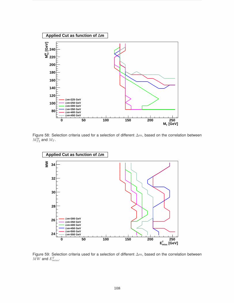
[GeV]TM0 50 100 150 200 250
[GeV
]W T
2M
80
100
120
140
160
180
200
220
240
m∆Applied Cut as function of
m=225 GeV∆m=250 GeV∆m=300 GeV∆m=350 GeV∆m=400 GeV∆m=450 GeV∆
m∆Applied Cut as function of
Figure 58: Selection criteria used for a selection of different ∆m, based on the correlation betweenMWT2 and MT .
[GeV]TmissE
0 50 100 150 200 250
MW
24
26
28
30
32
34
m∆Applied Cut as function of
m=300 GeV∆m=350 GeV∆m=400 GeV∆m=450 GeV∆m=500 GeV∆m=550 GeV∆
m∆Applied Cut as function of
Figure 59: Selection criteria used for a selection of different ∆m, based on the correlation betweenMW and ETmiss.
108

[GeV]TH100 150 200 250 300 350 400 450 500
]G
eV [
TH
/T m
iss
E
6
8
10
12
14
m∆Applied Cut as function of
m=300 GeV∆m=350 GeV∆m=400 GeV∆m=450 GeV∆m=500 GeV∆m=550 GeV∆
m∆Applied Cut as function of
Figure 60: Selection criteria used for a selection of different ∆m, based on the correlation betweenETmiss/
√HT and HT .
7.7 Systematic Uncertainties
The main sources of systematic uncertainties in this analysis are due to [52,71,89,90]:
• Inaccurate knowledge in the integrated luminosity.
• Efficiency in the identification and isolation of the leptons, as well as, trigger efficiencies.
• Jet Energy Scale (JES).
• The b-tagging efficiency.
Each of these sources is considered to be independent of the others and, for this reason, we add in
quadrature all the systematic uncertainties.
Table 21 shows the uncertainties due to the first two causes:
109

Source Value (%) Method
Luminosity 2.6 Obtained using the Van der Meer scans
performed in November 2012 [56].
Trigger and lepton 6 Obtained centrally from CMS by using a Tag-and-Probe
ID Efficiency method on Drell-Yan di-eletron and di-muon events [75,92]
Table 21: Source and value of systematic uncertainties taken from other studies.
Systematic uncertainties were propagated to any selection where the variable was used (see section
3.9).
7.8 Observed vs Expected Results
After applying the different selection criteria explained in previous sections, we find that the data is
well described by the SM backgrounds and we do not find any excess of events over background
indicating no presence of signal beyond the SM. Table 22 provides the expected number of events
and its uncertainties according to SM simulation and, the observed number of events obtained from
data.
7.8.1 Exclusion Plot
The exclusion plot shows the regions where observed data events minus background events are
lower than the SUSY signal expected events, at 95% confidence level. For this purpose, the following
parameter was defined [93]:
r=σ95%CLσSignal
(7.8.1)
Where:
σSignal: number of signal events.
σx%CL: number of observed data events minus background events are lower than the SUSY signal
expected events, at x% confidence level. In this analysis x = 95% was chosen as is usual in particle
physics.
To calculate the value of r for each of the combinations of stop and neutralino masses, the tool
developed for the combined analysis of Higgs was used [94]. The input to this tool is a card with the
number of observed events and the expected number of background and signal with their systematic
uncertainties (each is considered to be independent of the others).
110

∆m Observed Expected ± Stat ± SystRightSystLeft
100 17 14.6 ± 1.5 ± 3.62.9
125 110 109.4 ± 3.6 ± 15.214
150 162 152.6 ± 4.6 ± 16.513.9
175 49 47.9 ± 2.6 ± 4.84.2
200 90 81.8 ± 3.1 ± 16.316
225 199 179.3 ± 4.2 ± 32.933.4
250 257 232.4 ± 5.4 ± 26.330.7
275 171 175.9 ± 4.7 ± 12.412.2
300 146 142 ± 4.3 ± 10.110
325 113 111.3 ± 4.2 ± 10.311.5
350 89 82.1 ± 3.5 ± 7.48
375 51 44.5 ± 2.8 ± 6.26.6
400 49 52.8 ± 3 ± 4.75
425 33 33.5 ± 2.6 ± 2.22.3
450 24 25.3 ± 2.3 ± 2.12.1
475 21 22 ± 2.2 ± 2.22.6
500 14 18.4 ± 2.1 ± 2.62.8
525 3 4.6 ± 0.7 ± 0.40.5
550 3 4.5 ± 0.7 ± 0.40.5
575 3 4 ± 0.7 ± 0.40.5
600 3 3.5 ± 0.6 ± 0.40.5
625 1 2.5 ± 0.5 ± 0.30.4
650 2 1.6 ± 0.6 ± 0.40.5
675 6 5.6 ± 0.7 ± 0.50.6
700 1 1.1 ± 0.2 ± 0.30.3
725 1 0.8 ± 0.2 ± 0.10.1
750 1 0.7 ± 0.2 ± 0.10.1
Table 22: Comparison for each ∆m signal region between the expected and the observed number ofevents.
111

The exclusion plot is the contour with an r value of 1. Regions where r < 1 (regions contained under
the contour curve) correspond to the excluded regions.
Figure 61 shows the exclusion plot obtained with the present analysis. Comparison of our results
with the results from other analysis in the CMS experiment [75] are shown in Figures 62 and 63. Our
analysis excludes stop masses up to 660 GeV, for neutralino masses under 150 GeV. It also excludes
a parameter space region where ∆m = mt −mχ01
is lower than mass of the top. From the expected
results, it is concluded that this new analysis could be a powerful tool especially in regions where the
stop mass is high or in the region where ∆m is close to the top mass.
[GeV]t~m
200 300 400 500 600 700
[GeV
]0 1χ
m
50
100
150
200
250
300
350
400
=8 TeVs at -1 CMS: 19.5 fb
t0
1χ∼t0
1χ∼→
*t~
t~→pp
ObservedExpected
=8 TeVs at -1 CMS: 19.5 fb
Figure 61: Expected and observed exclusion plot obtained with this analysis. The excluded region isunder the curve.
112
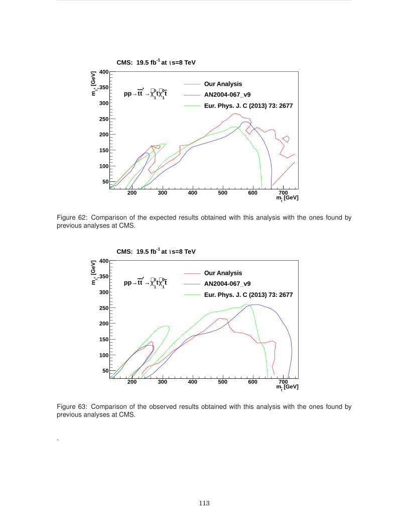
[GeV]t~m
200 300 400 500 600 700
[GeV
]0 1χ
m
50
100
150
200
250
300
350
400
=8 TeVs at -1 CMS: 19.5 fb
Our Analysis
AN2004-067_v9
Eur. Phys. J. C (2013) 73: 2677
t0
1χ∼t0
1χ∼→
*t~
t~→pp
Figure 62: Comparison of the expected results obtained with this analysis with the ones found byprevious analyses at CMS.
[GeV]t~m
200 300 400 500 600 700
[GeV
]0 1χ
m
50
100
150
200
250
300
350
400
=8 TeVs at -1 CMS: 19.5 fb
Our Analysis
AN2004-067_v9
Eur. Phys. J. C (2013) 73: 2677
t0
1χ∼t0
1χ∼→
*t~
t~→pp
Figure 63: Comparison of the observed results obtained with this analysis with the ones found byprevious analyses at CMS.
.
113

Chapter 8
CONCLUSIONS
Three different techniques were developed in the present analysis. They can be used independently
but for purposes of this analysis, they were used in a complementary way. These techniques are:
• Topological Reconstruction Using a Likelihood Function: this technique allowed us to re-
construct the topology of the event and define new topological variables that could be used in
the selection criteria. This method can be further improved to reconstruct the topology based
on all the background processes as well as on all the signal regions.
• Matrix Elements Method (MEM): since the computation time required to calculate the weight
from matrix elements is very high, we prefer not use this technique for full topological recon-
struction by iterating over all final states to find the best match to the topology studied. Instead,
we use it as a variable to discriminate between signal and background events.
• Variable Correlations: we use this method to find the reduced set of variables to define the
selection criteria. The analysis showed that a small set of variables could have a relative good
discrimination between signal and background.
The results obtained are consistent with the ones found by previous analyses. Even when the ob-
served excluded region is rather smaller for stop masses in the range of 500 GeV to 660 GeV, we
think this new analysis could be a powerful tool due to the expected results obtained. Although, no
new limits of exclusion are obtained, this analysis proves new techniques that can be further explored
as complementary to other analysis, specifically, we think the likelihood function and the selection
criteria based on correlations could be implemented using MVA. Additionally, we think that a data
driven study would be very useful since simulated samples are heavily used in the optimization of
each method (likelihood function, transfer function used in the MEM, selection criteria). Finally, sys-
tematic uncertainties due to PDF were not taken into account in this analysis because they are not
the dominant source of uncertainties, however, this is a further step that could be performed in order
to have a better accuracy in the results.
114

In conclusion, we have proven that methods focused in defining the topology of the events (not used
before in other analysis) are useful for the search for stops in the semileptonic channel and could be
further explored in combination with other techniques as for example boosted decision trees and could
be also used to study other processes. We hope that this study will stimulate further investigation in
this area.
115

Bibliography
[1] W. Beenakker, S. Brensing, M. Kramer, A. Kulesza and E. Laenen, “Super-Symmetric
Top and Bottom Squark Production at Hadron Colliders”, JHEP , 1008:098, 2010, doi:
10.1007/JHEP08(2010)098.
[2] The CMS Collaboration, “CMS Physics Technical Design Report Volume II: Detector
Performance and Software”, CERN/LHCC 2006-021 CMS TDR 8.2 26 June 2006.
[3] M. Papucci, T. Ruderman and A. Weiler, “Natural SUSY Endures”, JHEP , 1209:035,
2012, doi: 10.1007/JHEP09(2012)035.
[4] B. Howard. “Weak Scale Supersymmetry from Superfields to Scattering Events”, Ed.
Cambridge, ISBN-13: 978-0521857864.
[5] N. Sakai, “Naturalness in Supersymmetric Guts”, Z. Phys. C 11 (1981) 153,
doi:10.1007/BF01573998.
[6] R. K. Kaul and P. Majumdar, “Cancellation of Quadratically Divergent Mass Corrections
in Globally Supersymmetric Spontaneously Broken Gauge Theories”, Nucl. Phys. B 199
(1982) 36, doi:10.1016/0550-3213(82)90565-X.
[7] The CMS Collaboration, “Search for Top-Squark Pair Production in the Single-Lepton
Final State in pp Collisions at√s = 8 TeV”, Eur. Phys. J. C 73 2677, 2013.
[8] The ATLAS Collaboration, “Search for Top Squark Pair Production in Final States with
One Isolated Lepton, Jets, and Missing Transverse Momentum in√s = 8TeV pp Colli-
sions with the ATLAS Detector”, JHEP11(2014)118.
[9] L. Evans and P. Bryant, “LHC Machine”, 2008 JINST 3 S08001 doi:10.1088/1748-
0221/3/08/S08001.
[10] M. Lamont, “Status of the LHC”, Journal of Physics: Conference Series 455 (2013)
012001.
[11] The ATLAS Collaboration, “The ATLAS Experiment at the CERN Large Hadron Col-
lider”, 2008 JINST 3 S08003 doi:10.1088/1748-0221/3/08/S08003.
116

[12] The CMS Collaboration, “The CMS experiment at the CERN LHC, 2008 JINST 3
S08004 doi:10.1088/1748-0221/3/08/S08004.
[13] The ALICE Collaboration, “The ALICE experiment at the CERN LHC”, 2008 JINST 3
S08002 doi:10.1088/1748-0221/3/08/S08002.
[14] The LHCb Collaboration, “The LHCb Detector at the LHC”, 2008 JINST 3 S08005
doi:10.1088/1748-0221/3/08/S08005.
[15] The LHCf Collaboration, “The LHCf detector at the CERN Large Hadron Collider”, 2008
JINST 3 S08006 doi:10.1088/1748-0221/3/08/S08006.
[16] The TOTEM Collaboration, “The TOTEM Experiment at the CERN Large Hadron Col-
lider”, 2008 JINST 3 S08007 doi:10.1088/1748-0221/3/08/S08007.
[17] The MoEDAL Collaboration, “The Physics Programme of the MoEDAL Experiment at
the LHC”, arXiv:1405.7662v4.pdf.
[18] T. Lenzi, “Development and Study of Different Muon Track Reconstruction Algorithms for
the Level-1 Trigger for the CMS Muon Upgrade with GEM Detectors”, arXiv:1306.0858
CERN-THESIS-2013-042.
[19] G. Antchev, “Luminosity-Independent Measurement of the Proton-Proton Total Cross
Section at√s = 8 TeV”, Phys. Rev. Lett. 111, 012001 (2013).
[20] The CMS Collaboration, “Projected Performance of an Upgraded CMS Detector at the
LHC and HL-LHC: Contribution to the Snowmass Process”,
http://arxiv.org/pdf/1307.7135.pdf
[21] The CMS Collaboration, “Study of Pileup Removal Algorithms for Jets”, CMS PAS JME-
14-001.
[22] W.J. Stirling, private communication, “Ratios of LHC Parton Luminosities”,
http://www.hep.ph.ic.ac.uk/~wstirlin/plots/lhclumi7813_2013_v0.pdf
[23] The CMS Collaboration,“CMS Luminosity-Public Results”,
https://twiki.cern.ch/twiki/bin/view/CMSPublic/LumiPublicResults#Pileup_distribution
[24] K.A. Olive et al. (Particle Data Group), “The Review of Particle Physics”, Chin. Phys. C,
38, 090001 (2014).
[25] The CMS Collaboration, “CMS Physics Technical Design Report Volume I: Detector
Performance and Software”,
CERN/LHCC 2006-001 CMS TDR 8.1 2 February 2006.
[26] The CMS Collaboration, “The Tracker System Project Technical Design Report”,
CERN/LHCC 98-6 CMS TDR 5 15 April 1998.
117

[27] B. Isildak, “Measurement of the differential dijet production cross section in proton-
proton collisions at√s=7 TeV”, arXiv:1308.6064.
[28] The CMS Collaboration, “CMS ECAL Technical Design Report”,
CERN/LHCC 97-33 CMS TDR 4 15 December 1997.
[29] The CMS Collaboration, “CMS HCAL Technical Design Report”,
CERN/LHCC 97-31, CMS TDR 2, 20 June 1997.
[30] Cavallo, Benettoni and Conti, “Test of CMS Muon Barrel Drift Chambers with Cosmic
Rays”, CMS-NOTE-2003-017.
[31] P. Pierluigi, “CMS Resistive Plate Chamber overview, from the present system to the
upgrade phase I”, 2013 JINST 8 P04005.
[32] M. Felcini, “The Trigger System of the CMS Experiment”,
Nuclear Instruments and Methods in Physics Research: Volume 598, Issue 1, 1 January
2009, Pages 312–316.
[33] CMSSW Reference Manual.
http://cmssdt.cern.ch/SDT/doxygen/
[34] ROOT.
http://root.cern.ch/drupal/
[35] CERN, “The Grid: A system of tiers”,
http://home.web.cern.ch/about/computing/grid-system-tiers
[36] The CMS Collaboration, “Missing Transverse Energy Performance of the CMS Detec-
tor”, 2011 JINST 6 P09001 doi:10.1088/1748-0221/6/09/P09001.
[37] The CMS Collaboration, “Performance of the CMS missing transverse momentum re-
construction in pp data at√s = 8 TeV”, J. Instrum. 10 (2015) P02006 DOI 10.1088/1748-
0221/10/02/P02006.
[38] The CMS Collaboration, “CMS Twiki on Calo Towers”,
https://twiki.cern.ch/twiki/bin/view/CMSPublic/SWGuideCaloTowers
[39] The CMS Collaboration, “Performance of electron reconstruction and selection with the
CMS detector in proton-proton collisions at√s = 8 TeV”, arXiv:1502.02701.
[40] W. Adam, “Reconstruction of electrons with the Gaussian-sum filter in the CMS tracker
at the LHC”, doi:10.1088/0954-3899/31/9/N01.
[41] The CMS Collaboration, “CMS Twiki on Egamma Cut Based Identification”,
https://twiki.cern.ch/twiki/bin/view/CMS/EgammaCutBasedIdentification
[42] The CMS Collaboration, “Performance of muon reconstruction and identification in pp
collisions at√s=7 TeV”, CMS PAS MUO-10-004.
118

[43] The CMS Collaboration, “CMS Twiki on Muon Id”,
https://twiki.cern.ch/twiki/bin/view/CMSPublic/SWGuideMuonId
[44] Soyez, “The SISCone and Anti-kt Jet Algorithms”, BNL-81350-2008-CP .
[45] Soyez, Cacciari and Salam, “The Anti-kt Jet Clustering Algorithm”, JHEP04(2008)063.
[46] The CMS Collaboration, “Performance of the Particle-Flow jet identification criteria us-
ing proton-proton collisions at√s = 8 TeV”, CMS AN-14-227.
[47] The CMS Collaboration, “Identification of b-quark Jets with the CMS Experiment”, 2013
JINST 8 P04013.
[48] The CMS Collaboration, “Performance of b tagging at√s = 8 TeV in multijet, tt and
boosted topology events”, CMS PAS BTV-13-001.
[49] Coccaro, J. Andrea, “Track Reconstruction and b-Jet Identification for the ATLAS Trigger
System”, Phys.Conf.Ser. 368 (2012) 012034 arXiv:1112.0180 [hep-ex].
[50] A. Onofre, “Top Quark Couplings and Search for New Physics at the LHC”, 2013 J.
Phys.: Conf. Ser. 447 012030.
[51] The CMS Collaboration, “Commissioning of the Particle-Flow Event Reconstruction with
the first LHC Collisions Recorded in the CMS Detector. CMS Physics Analysis Sum-
mary CMS-PAS- PFT-10-001, 2010.
[52] The CMS Collaboration, “Determination of Jet Energy Calibration and Trans-
verse Momentum Resolution in CMS”, 2011 JINST 6 P11002 doi:10.1088/1748-
0221/6/11/P11002.
[53] L. Gouskos, “Search for supersymmetry in events with a single lepton, jets and missing
transverse energy with the CMS detector at LHC”, CERN-THESIS-2014-138.
[54] The CMS Collaboration, “CMS Twiki on MET Optional Filters”,
https://twiki.cern.ch/twiki/bin/viewauth/CMS/MissingETOptionalFilters
[55] M. Buchmann, “Search for Physics Beyond the Standard Model in the Opposite-Sign
Same-Flavor Dilepton Final State with the CMS Detector”, CERN-THESIS-2014-04
[56] The CMS Collaboration, “CMS Luminosity Based on Pixel Cluster Counting - Summer
2013 Update”, CMS PAS LUM-13-001.
[57] T. Theveneaux-Pelzer and J. Fernandez, “Leptons + systematic uncertainties”, ATL-
PHYS-PROC-2013-330 12/12/2013.
[58] R. Eusebi, “Jet energy corrections and uncertainties in CMS: reducing their impact on
physics measurements”, 2012 J. Phys.: Conf. Ser. 404 012014.
[59] A. Kalogeropoulos, “Search for direct stop pair production at the LHC with the CMS
experiment”, CMS-TS-2014-038, CERN-THESIS-2013-347.
119

[60] Denis Perret - Gallix, “Computational particle physics for event generators and data
analysis”, 2013 J. Phys.: Conf. Ser. 454 012051.
[61] MadGraph.
http://madgraph.hep.uiuc.edu/
[62] PYTHIA.
http://home.thep.lu.se/~torbjorn/Pythia.html
[63] Geant4.
http://geant4.cern.ch/
[64] D. Abbaneo, G. Abbiendi and M. Abbrescia, “A New Boson with a Mass of 125 GeV
Observed with the CMS Experiment at the Large Hadron Collider”, Science 12/2012;
338(6114):1569-1575. DOI:10.1126/science.1230816.
[65] The K2K Collaboration, “Measurement of Neutrino Oscillation by the K2K Experi-
ment”, Phys. Rev. D 74 (2006) 072003, doi:10.1103/PhysRevD.74.072003 , arXiv:hep-
ex/0606032.
[66] The Planck Collaboration, “Planck 2013 Results. XVI. Cosmological parameters”, As-
tron. Astrophys. (2014) doi:10.1051/0004-6361/201321591 , arXiv:1303.5076.
[67] Locco, Pato & Bertone. “Evidence for Dark Matter in the Inner Milky Way”, Nature
Physics, 11, 245–248 (2015) doi:10.1038/nphys3237.
[68] V. Rubakov, “Cosmology”, arXiv:1504.03587v1.
[69] M. Vidal, “Search for Gluino-Mediated Sbottom Production”, PRL 102, 221801 (2009).
[70] H. K. Dreiner, T. Stefaniak, “Bounds on R-parity Violation from Resonant Slepton Prod-
uct ion at the LHC”, DOI 10.1103/PhysRevD.86.055010.
[71] The CMS Collaboration, “Interpretation of Searches for Supersymmetry with Simplified
Models”, Phys. Rev. D 88 (2013), 10.1103/PhysRevD.88.052017.
[72] The CMS Collaboration, “CMS Twiki on CMS Supersymmetry Physics Results”,
https://twiki.cern.ch/twiki/bin/view/CMSPublic/PhysicsResultsSUS
[73] The ATLAS Collaboration, “ATLAS Twiki on ATLAS Supersymmetry (SUSY) searches”,
https://twiki.cern.ch/twiki/bin/view/AtlasPublic/SupersymmetryPublicResults.
[74] D. Teyssier, “LHC results and prospects: Beyond Standard Model”, arXiv:1404.7311v1.
[75] The CMS Collaboration, “Search for direct stop pair production in the semi-leptonic
channel at 8 TeV”, CMS AN-14-067.
[76] The CMS Collaboration,“Exclusion limits on gluino and top-squark pair production in
natural SUSY scenarios with inclusive razor and exclusive single-lepton searches at√s
= 8 TeV.”, CMS PAS SUS-14-011.
120

[77] V. Martinez,“Recent results on SUSY searches from CMS”,
http://cms.web.cern.ch/news/recent-results-susy-searches-cms
[78] The CMS Collaboration,“Search for supersymmetry in pp collisions at√s = 8 TeV in
events with three leptons and at least one b-tagged jet”, CMS-PAS-SUS-13-008.
[79] The CMS Collaboration,“Search for new physics in events with same-sign dileptons and
jets in pp collisions at 8 TeV”, CMS-PAS-SUS-13-013.
[80] The CMS Collaboration,“Search for electroweak production of charginos, neutralinos,
and sleptons using leptonic final states in pp collisions at 8 TeV”, CMS-PAS-SUS-13-
006.
[81] The CMS Collaboration,“Search for RPV SUSY in the four-lepton final state”, CMS-
PAS-SUS-13-010.
[82] A. Aubin, “CMS Twiki on Babytuples for stop”,
https://twiki.cern.ch/twiki/bin/viewauth/CMS/StopBabiesV2.
[83] Bai,Cheng, “Stop the Top Background of the Stop Search”, arXiv:1203.4813v1
[84] The CMS Collaboration, “CMS Twiki on Frontier Conditions”,
https://twiki.cern.ch/twiki/bin/view/CMSPublic/SWGuideFrontierConditions
[85] O. Mattelaer, “Starting MadWeight”,
https://cp3.irmp.ucl.ac.be/projects/madgraph/wiki/StartingMadWeight
[86] J.C. Estrada, “Maximal Use of Kinematic Information for Extracting Top Quark Mass in
Single-Lepton ttbar Events”,
http://www-d0.fnal.gov/Run2Physics/top/top_public_web_pages/top_dissertations.html
[87] A. Jack (UCSB), “b-tagging Performance at High pT in Semi-leptonic Top-Enriched
Events with 6.2 fb−1 of 2012 Data”.
[88] The CMS Collaboration, “Measurement of the top-quark mass in tt events with lep-
ton+jets final states in pp collisions at√s = 8 TeV”, CMS PAS TOP-14-001
[89] The CMS Collaboration, “CMS Twiki on Single Electron efficiencies and Scale-Factors”,
https://twiki.cern.ch/twiki/bin/view/Main/EGammaScaleFactors2012
[90] The CMS Collaboration, “CMS Twiki on Methods to apply b-tagging efficiency scale
factors”,
https://twiki.cern.ch/twiki/bin/viewauth/CMS/BTagSFMethods
[91] The CMS Collaboration, “CMS Twiki on Tag and Probe measurements of data/MC effi-
ciency scale factors (SF)”,
https://twiki.cern.ch/twiki/bin/viewauth/CMS/MuonTagAndProbe
121

[92] The CMS Collaboration, “CMS Twiki on TOP Systematic Uncertainties”,
https://twiki.cern.ch/twiki/bin/viewauth/CMS/TopSystematics
[93] C. Wymant, “Brazil-Band Plots For Dummies”,
lapth.cnrs.fr/pg-nomin/wymant/BrazilBandPlot.pdf
[94] The CMS Collaboration, “CMS Twiki on Higgs Combination”,
https://twiki.cern.ch/twiki/bin/viewauth/CMS/
SWGuideCMSDataAnalysisSchool2014HiggsCombPropertiesExercise
[95] Madgraph team, “Card Examples”,
http://madgraph.hep.uiuc.edu/EXAMPLES/proc_card_examples.html
122

Appendix A
Datasets used in this Analysis
Table 23 shows a list of the datasets that were used in this analysis, In this table, AOD stands for
Analysis Object Data, Reco for Reconstructed Data and Run A,B and C for the periods of time of data
taking (see section 2.2.2).
Single lepton datasets
/SingleMu/Run2012A-13Jul2012-v1/AOD
/SingleMu/Run2012A-recover-06Aug2012-v1/AOD
/SingleMu/Run2012B-13Jul2012-v1/AOD
/SingleMu/Run2012C-24Aug2012-v1/AOD
/SingleMu/Run2012C-PromptReco-v2/AOD
/SingleMu/Run2012C-EcalRecover-11Dec2012-v1/AOD
/SingleElectron/Run2012D-PromptReco-v1/AOD
/SingleElectron/Run2012A-13Jul2012-v1/AOD
/SingleElectron/Run2012A-recover-06Aug2012-v1/AOD
/SingleElectron/Run2012B-13Jul2012-v1/AOD
/SingleElectron/Run2012C-24Aug2012-v1/AOD
/SingleElectron/Run2012C-PromptReco-v2/AOD
/SingleElectron/Run2012C-EcalRecover-11Dec2012-v1/AOD
/SingleElectron/Run2012D-PromptReco-v1/AOD
Table 23: Summary of single lepton datasets used [75].
123

Appendix B
Implementation of the Matrix Element
Method Using MadWeight
There is a program called MadWeight that is widely used in the world by the particle physics commu-
nity, developed by the same team that designed and implemented MadGraph. This software calcu-
lates the weight given by the method of matrix elements and must be configured via multiple cards
to define the type of process, the center of mass, the number of integration points and the transfer
function among others [95]. The input file for this program is given in lhco format and contains the
information of the four-vectors of all objects in the final state.
Figure 64 shows an example of a LHCO file, where the meaning of each of the columns (left to right)
is given by:
1. Number of line
2. Particle type (4: jet, 1:electron, 2:muon, 6: ETmiss)
3. η component.
4. φ component.
5. pT component.
6. M (mass) component.
7. Number of tracks
8. b-jet (2:true, 0:false)
9. Had/EM (ratio between the energy deposited in the hadronic calorimeter to the one deposited
in the electromagnetic calorimeter)
10. dummy variable (for user)
124

11. dummy variable (for user)
Figure 64: LHCO file example.
The matrix elements calculation is computationally very heavy. A typical CPU time to process one
event is about one minute. In order to reduce the computing time, the number of integration points
versus the matrix element calculation was studied. The study allowed us to define the minimum
number of integration points to be used. The default number of integration points is 50000. Figure 65
shows the weight obtained by MADWEIGHT as a function of integration points. After 10000 iterations
we find that the value of the weight has converged to a stable point (plateau). We used this value as
the minimum number of integration points used.
Figure 65: Weight (left) and relative error (right) obtained with MadWeight with respect to the numberof integration points used in the calculation.
A second improvement made to optimize the computing time for calculating the matrix elements was
to run MADWEIGHT with crab.
The advantage of this improvement is that it allows to run in parallel using the GRID.
We give a brief documentation about this implementation since no documentation is available:
• Run CRAB in mode no-dataset.
• Run a script from CRAB (see Figure 66).
125

Figure 66: .cfg Crab Card.
• From the script to call the code and give to it the job number. The job number is given by CRAB
to the script as $1.
• In the code use the job number to select the range of events to be analyzed.
• Copy MadWeight inside a folder called data that is within the src folder of CMSSW. This should
be done as CRAB uploads everything inside data. An important observation is that the size
should not exceed 100MB.
• Copy the preselected samples to EOS.
• To run MadWeight it is important to have into account that once the code is running in the GRID,
the point from which it runs is the src folder of CMSSW.
126

Appendix C
Statistical Uncertainties
Statistical uncertainties are used to consider fluctuations at 1σ level in the process of selecting the
correlation selection criteria (this is explained in section 7.6). For this reason, we developed the
method described below for calculating the statistical uncertainties for each of the cells that are used
with the correlations method.
The number of events is given by:
N=σLNACNBC
(C.0.1)
where:
N : number of events normalized to luminosity
σ : cross section
L : integrated luminosity
NAC : number of simulated events after cuts
NBC : number of simulated events before cuts
To differentiate events that are independent, we make the substitution:
A = NBC −NAC (C.0.2)
and obtain:
N=σLNAC
A+NAC(C.0.3)
we can calculate the statistical error using:
127

(∆N)2=(∂N
∂NAC)2(∆NAC)
2 + (∂N
∂A)2(∆A)2 (C.0.4)
from here we get:
(∆N)2=(σLA
N2BC
)2NAC + (σLNACN2BC
)2A (C.0.5)
and rearranging some terms:
(∆N)2=(σL
NBC)2NAC + (
σL
NBC)2N2AC
NBC(C.0.6)
thus, it is possible to define the weights:
w1=(σL
NBC)2 (C.0.7)
w2=σL
NBC√NBC
(C.0.8)
with these weights the statistical error can be obtained as follows:
1. w3 =∑
w1 over all the simulated events after cut(s).
2. w4 =∑
w2 over all the simulated events after cut(s).
3. ∆N =√
w3 + w24
128

Appendix D
Work Performed by the Author at
CMS
The work performed, by the author of this thesis, at CMS experiment has been mainly focused in
RPCs and b-tagging.
The activities that have been executed are:
• Development of HVScan tool for the RPCs. This tool is composed by several modules that can
be run in a sequence to obtain the following results:
– Fit of the curve given by Efficiency vs High Voltage of Operation (Sigmoid function is used).
– Fit of the curve given by Cluster Size vs High Voltage of Operation (Exponential function is
used).
– Plots of the fits mentioned above. In these plots are shown the working point, the knee
(both of these according with the definition given by the CMS-RPC group), and the points
from where the fit is obtained. It is also possible to plot the working point per channel but
this information is not the result of any of these modules.
– Classification of the rolls according to the criteria defined by the CMS-RPC group.
– ROOT file with the histograms of several distributions.
– Web Page with the plots and relevant information about the fit. All the information about
this tool can be found at:
https://twiki.cern.ch/twiki/bin/view/Sandbox/CMSRPCHVSCANTOOL
• Development of an analyzer to study the possible differences between RPC points obtained by
extrapolation from segments, and RPC points obtained by extrapolation from tracks.
• Development of a producer of new RPC extrapolated points from tracks. This code was devel-
oped to reduce the impact of the relative high pileup in the measure of the RPC efficiency.
129

I also had the opportunity of guiding the work of a M.Sc. student in the RPC reshuffling study, as well
as, I worked with the b-tagging group in improving one of the methods (System8) used to measure
the efficiency of the algorithms to identify b-quarks. Additionally, I was tutor of one of the courses
given to teach the use of the platform developed within the experiment for physics analysis (Physics
Analysis Tool PAT). Finally, I paid my service as a data manager shifter to supervise the performance
of the RPCs during some of the runs and I was also a central shifter monitoring the quality of the data.
130