Second Grade Internship Report

DYNAMIC PARAMETERS IDENTIFICATIONA BISECTION APPROACH BASED ON INTERVAL ANALYSIS

Institute Tutor:

Luc JAULIN

Enterprise Supervisor:

Julien ALEXANDRE DIT SANDRETTO

Alexandre CHAPOUTOT

Intern: Lei ZHU

Major: Robotique

October 9, 2016

Resume

Le rapport se concentre sur les sujets des problemes d’identification des

parametres sur un aeroglisseur. Une methodologie basee sur l’analyse

d’intervalle est donnee par l’auteur. Comme le travail de son stage, il

s’est adonne sur la conception de l’algorithme dans le but d’identifier

les parametres avec les mesures indiquees. L’analyse par intervalles

est utilisee pour estimer la borne de valeur reelle. Une methode de

Runge-Kutta est egalement fait usage de calculer tous les etats. L’auteur

utilise en meme temps la methode de bissection pour rechercher dans

l’espace de solution. Compte tenu des inconvenients de la premiere ver-

sion de l’algorithme, l’auteur a fait une optimisation sur l’algorithme.

En consequence, l’algorithme designee optimise bien resolu le probleme.

Les parametres avec lesquels la simulation se fait tous se trouvent a la fin.

L’auteur suggere que cet algorithme est bien marche pour un probleme

dynamique d’identification des parametres. Considerant qu’il lance tres

lentement, c’est necessaire d’optimiser l’algorithme pour une meilleure

performance. Un algorithme assez rapide contribuera beaucoup a la tech-

nologie de l’industrie robotique.

Mots cles: Analyse intervalle; Identification de parametres; Controle;

Bisection

Abstract

This report focuses on the topics of a parameter identification problem

build on a hovercraft. A methodology based on interval analysis is given

by the author. As the job of his internship, he worked on the design of

algorithm for the purpose of identifying the parameters with given mea-

surements. Interval analysis is used to estimate the range of real value.

A Runge-Kutta method is also made use of to calculate all the states.

The author meanwhile utilize bisection method to search in the solution

space. Considering the disadvantages of the first version of algorithm,

the author did an optimization. As consequence, the optimized algo-

rithm well solved the problem. The parameters with which the simula-

tion is done are all found at last. The writer suggests that this algorithm is

well-worked for a dynamic parameter identification problem. Whereas it

launches very slowly. It is necessary to optimize the algorithm for faster

performance. A fast enough algorithm will contribute a lot to the heated

technology of advanced robot industry.

Keywords: Parameter Identification; Interval Analysis; Low of Control;

Bisection

Contents

1 Introduction 1

1.1 Organization of Internship . . . . . . . . . . . . . . . . . . . . . . . . 1

1.1.1 ENSTA Paristech . . . . . . . . . . . . . . . . . . . . . . . . . 1

1.1.2 Robotic Laboratory of ENSTA Paristech . . . . . . . . . . . . . 2

1.2 Subject Background . . . . . . . . . . . . . . . . . . . . . . . . . . . . 2

1.3 Missions to Realize . . . . . . . . . . . . . . . . . . . . . . . . . . . . 3

2 Preparation Work 5

2.1 Theoretical Basis . . . . . . . . . . . . . . . . . . . . . . . . . . . . . 5

2.1.1 Model-based Control and Parameters Identification . . . . . . . 5

2.1.2 Interval Analysis . . . . . . . . . . . . . . . . . . . . . . . . . 6

2.1.3 Runge–Kutta Methods and DynIbex . . . . . . . . . . . . . . . 7

2.2 Mathematical Model of the Hovercraft . . . . . . . . . . . . . . . . . . 7

2.3 Parameter Selection . . . . . . . . . . . . . . . . . . . . . . . . . . . . 9

2.4 Designed Scenarios . . . . . . . . . . . . . . . . . . . . . . . . . . . . 11

3 Constructed Algorithms 13

3.1 First Algorithm . . . . . . . . . . . . . . . . . . . . . . . . . . . . . . 13

3.2 Optimized Algorithm . . . . . . . . . . . . . . . . . . . . . . . . . . . 14

3.3 Simulation Data Generation . . . . . . . . . . . . . . . . . . . . . . . 15

3.4 Real Experiment . . . . . . . . . . . . . . . . . . . . . . . . . . . . . 15

4 Results and Conclusion 16

4.1 Results . . . . . . . . . . . . . . . . . . . . . . . . . . . . . . . . . . . 16

1

4.2 Conclusion . . . . . . . . . . . . . . . . . . . . . . . . . . . . . . . . 17

4.3 Acquisition . . . . . . . . . . . . . . . . . . . . . . . . . . . . . . . . 17

4.4 Future Application . . . . . . . . . . . . . . . . . . . . . . . . . . . . 17

5 Acknowledgment 19

2

Chapter 1: Introduction

1.1 Organization of Internship

1.1.1 ENSTA Paristech

ENSTA ParisTech, or so-called Ecole Nationale Superieure de Techniques Avancees

in French, is a teaching and public research institution that is self-governed under the

supervision of the Ministry of Defence. It enjoys a special position in the French ed-

ucation system. It belongs to one of the most important schools of engineering in the

country.

ENSTA ParisTech offers its students a general training in engineering in order to en-

able them to design, implement and manage complex technical projects, while meeting

economic constraints in an international environment. In this perspective, the Institute

offers training high scientific and technological level, which is constantly updated to

keep pace with changes in advanced technology, and supplemented by the languages,

humanities and skills in business life such as law, communication, economics, account-

ing and management.

Research is another main task of ENSTA. Its five departments conduct research in

many areas, in partnership with French universities, European and international and

public research organizations. Many CNRS research staff, INSERM and the Ecole

Polytechnique also worki on ENSTA’s own professors sides of the institute. The depart-

ments carry out research mainly applied with industrial problems, but are also involved

in the fundamental developments in the interest of scientific knowledge and aiming at

technological breakthroughs. The research provides a dynamic contribution to the edu-

cational work of the school, behind its connection with scientific state-ot-the-art.

In December 2010, ENSTA Paristech and ENSTA Bretagne (former Ensieta), two

engineering schools had created the complementary ENSTA group to enhance training

and high-level research activities. This group combines two schools with their recog-

nized performances in their areas of expertise: energy, transportation, marine engineer-

ing and large industrial systems. It offers two schools on development of an ambitious

strategy of growth and international exposure for their engineering education and re-

search activities. In a highly competitive environment for higher education, the height

1

and visibility are key growth factors, and the creation of the ENSTA Group fits into this

perspective.

1.1.2 Robotic Laboratory of ENSTA Paristech

The Robotics Laboratory, known more formally as Autonomous Systems and Robotics

Team, do researches focused on mobile robot navigation, perception, vision board, mo-

tor learning and human-robot interaction. Their primary objective is the application

of machine learning to real-world, such as service and assistive robotics, humanoid

robotics, intelligent vehicles, and security.

The team was founded by Jean-Christophe Baillie, and as a result of his work on

control architectures, he introduced the language of the interface URBI to control the

robot. This language was also developed by GOSTAI, a spin-off company he created,

now bought by Aldebaran Robotics.

The Robotics Laboratory is part of Computer Science and System Engineering Lab-

oratory of ENSTA-Paristech in Paris, France. Several team members are also part of

the team INRIA / ENSTA-Paristech FLOWERS, co-located in Palaiseau and Bordeaux,

which focuses on developmental robotics.

1.2 Subject Background

The robotic laboratory of ENSTA Paristech has recently designed a remote con-

trolled hovercraft( Figure 1.1 ), which is equipped with electronic components as well

as an Arduino board for central control.

The construct of this drone like robot is based on dynamic model [1], which is an

approximation of a real hovercraft. Even though it is a simplified model, it has almost

all the most important characteristics of a hovercraft. It is necessary to build a method

for identification of dynamic parameters (mass, inertia, friction coefficients, etc.) so

that the model is as close to reality as possible [2].

In this area, we work extensively with interval analysis which allows us to use the

range of value in place of a solid number.This is because of two reasons: on one side, in

the real environment all the acquired data is with errors; on the other side, all component

2

Figure 1.1: Simplified Model of a Hovercraft

have little motion when the hovercraft flies. Using this mathematical tool,all data are

represented by a range, thus it is possible to make sure the calculation of all parameters

and measurements well fits the reality.

Once such a model obtained and validated by the measurements, it will be inter-

esting to define a law of control (or several), simply and robustly, for the hovercraft to

accomplish a path under aimless situation (which means without sensor) or even more

independent to pass an area with barriers without any prior knowledge of this area.

This can also contribute a good way of the heated unmanned issue. In addition, with

more than one path, it is easier to get more state data, which helps a lot to judge if the

parameters are correct.

1.3 Missions to Realize

• Define the measurements to be performed for the identification of parameters;

There are several measurements for the stare equations, in which some are very

useful while some not, some are possible to measure and the others not. So the

3

first thing is to choose the measurements to use.

• Choose the parameters to calculate by orders;

The stare equations are represented with help of lots of parameters, but the co-

efficient of each parameter is rather different. In a mathematical way, all the

parameter should be chose by an order of importance.

• Acquire the measurements (with Arduino program and experiments);

This mission allows us to get data for calculation, but the data can be generated

randomly as a simulation at the first time.

• Develop a tool for the identification of dynamic parameters;

Write an algorithm or a program that identify the parameters.

• Design one or more control laws based on the simulation hovercraft.

On control law is not enough, should more different path be designed. And repeat

the steps on the new control laws helps us get more data, which can be used for

correct the errors and optimize the parameters.

4

Chapter 2: Preparation Work

2.1 Theoretical Basis

2.1.1 Model-based Control and Parameters Identification

Model-based control is a kind of robot control method based on the theoretical

physics model [1] [2] [3]. In the research of intelligent robots, a very important subject

is how to correctly establish the mathematical model of the manipulated object, in or-

der to construct a corresponding control [4].

The model is described by a series of parameters. Typically, they can be identified

by static parameters identification methods [3] [5]:

1. Physical experiments, in which we measure the physics parameter directly.

2. Computer aided design (CAD) techniques, which means a graphic simulation by

computer.

3. Black Box method, which use a mathematical tool to analyze the function be-

tween input and out put.

However, none of the static methods can adapt to the requirements of high accuracy

in a real-time environment [6], While dynamic parameters can be used for describing the

dynamic kinematics model of a robot, more precisely. They are important for advanced

control algorithms based on models [7], which is because they have great influence on

the validation of simulation results as well as the accuracy of algorithms designed for

path planning. Nowadays, the requirements to accuracy and reliability of the system

becomes increasingly strict, especially in the field of mechatronics robotics.

With all the parameters of a model identified, we can do all kinds of experiments by

simulation on the computer. And if these parameters are accurate enough, there will be

no difference between the results of simulation and actual experiments. Thus we can

build a perfect control algorithm for the robots.

However, the ideal situation does not exist [8]. The parameters have uncertainties,

and can be very sensitive to the errors. Therefore we utilize a mathematical tool which

5

is called Interval Analysis [9].

2.1.2 Interval Analysis

In mathematics, interval analysis is a method for automated error estimation on the

basis of closed intervals . In this case, x is not considered as an exactly known real

variable, but a range which can be limited by two numbers a and b. X can lie between a

and b or can also assume one of the two values. This range corresponds mathematically

to the interval [a, b]. A function f, which depends on such an uncertain x, can not be

evaluated exactly. Finally, it is not known that numerical value should actually be used

within [a, b] for x. Instead, the smallest possible interval [c, d] is determined, which

contains the possible function values f (x) for all x ∈ [a, b]. By means of a targeted

estimation of the end points c and d, a new function is obtained, which is a reflection

from intervals to intervals [10].

This concept is suitable, among other things, for the treatment of rounding errors

directly during the calculation and in case of uncertainties in the knowledge of the exact

values of physical and technical parameters. The latter often result from measurement

errors and component tolerances. Moreover, interval analysis can help to obtain reliable

solutions of equations and optimization problems.

Figure 2.1 is an example of interval analysis application done on the platform of

Ibex, a C++ library based on interval arithmetic for constraint processing over real

numbers. The values at first not very accurate as represented in the blue range. But

after a few steps calculation, the intervals shrink to yellow range and finally even in the

black line at the center of the yellow range.

Interval analysis can also be used for error analysis in order to control the rounding

errors resulting from each calculation [11]. The advantage of interval arithmetic is that

after each operation, there is a gap which comprises reliably the true result. The distance

between the ends of the range gives the current calculation rounding errors directly:

Error = abs(a − b) to an interval [a, b]. Calculation with the two bounds is both clear

and easy.

6

Figure 2.1: an Application of Interval Analysis

2.1.3 Runge–Kutta Methods and DynIbex

The Runge–Kutta methods are a family of implicit and explicit iterative methods [12],

which includes the well-known routine called the Euler Methods, used in temporal dis-

cretization for the approximate solutions of ordinary differential equations.

DynIbex is a plug-in of Ibex library for constraint processing over real numbers. It

offers a set of validated numerical integration methods based on Runge-Kutta schemes

to solve initial value problem of ordinary differential equations and for DAE in Hessen-

berg index 1 form.

2.2 Mathematical Model of the Hovercraft

We work directly on the hovercraft model designed by robotic laboratory of ENSTA

Paristech [1]. This is a reduced model, but with a complex behavior. The state equations

7

can be given as follow:

u = vr +1

mX (2.1a)

v = −ur + 1

mY (2.1b)

r =1

IzN (2.1c)

x = cos(ψ)u− sin(ψ)v (2.1d)

y = sin(ψ)u+ cos(ψ)v (2.1e)

ψ = r (2.1f)

X, Y and N are denoted as the force and the moments in the whole system. They

may come from the propulsion of motor, the air resistance , the friction on the ground

or the damping of each rudder. X and Y are represented on the horizon plat, while N

stands for the vertical direction. All the 3 variables are orthogonal. They are given by

these equations:

X = Fu − µNf(u)u

u2 + v2− 1

2ρCdSu

√u2 + v2u−D11u (2.2a)

Y =1

4ACLSvCFuδ − µNf(v)

v

u2 + v2− 1

2ρCdSv

√u2 + v2v −D22v (2.2b)

N = −L 1

4ACLSgCFuδ −D33r (2.2c)

With constraints:

Fu = CFuW2 (2.3a)

CFu = CδρD4 (2.3b)

A = πRh2 (2.3c)

Rh =1

2D (2.3d)

In the equations (1)-(3), we introduce many symbols, in which u means the veloc-

ity of hovercraft in x-axis direction, as well as v in y-axis direction. r stands for the

8

angular velocity, which is useful when the hovercraft turns around. x, y and ψ are the

position coordinate and angular direction corresponding respectively to u, v and r. f is

a regularization function to avoid a discontinuity between the static and sliding friction.

δ represent the law of control for path-finding. Except all these 8 variables, all the other

symbols we use here are the parameters. Their physic meaning and units are shown in

the following table:

Table 2.1: Parameters of Hovercraft Model.Parameter Physic Representation Unit

m mass kgD propeller diameter mL distance between gravity center and the rudder aerodynamic center mW rotational speed s−1

Iz moment of inertia according to z-axis kg ·m2

Cd air resistance coefficient −CL rudder lift coefficient rad−1

CFu propulsion coefficient −Cδ dimensional propulsion coefficient −Su front area surface m2

Sv side area surface m2

Sg rudder area surface m2

A propeller-rotation-generated surface m2

ρ air density kg ·m−3

µ friction coefficient −xg x-coordinate of the gravity center myg y-coordinate of the gravity center mD11 damping according to x-axis kg · s−1

D22 damping according to y-axis kg · s−1

D33 damping according to z-axis kg · s−1

2.3 Parameter Selection

Fortunately, for such a huge group of equations, we have some common sense to

help us determine the an approximate range of several parameters. For example, even if

we do not know exactly the numerical value of m (mass), we can get it from a weighing

scale. Consider that this hovercraft is rather light, our priory experience tell us this in-

dication error will be less than 0.5 kg. We apply this technique to all the parameters, we

can draw a word sketch of the whole system. Then we calculate the partial derivative of

these equations, hence we get partial differential coefficients for all parameters, namely,

the significance of each parameter to all the variables. Under this approach, we divide

all the parameters into 3 categories: very important, negligible and the others (Table

9

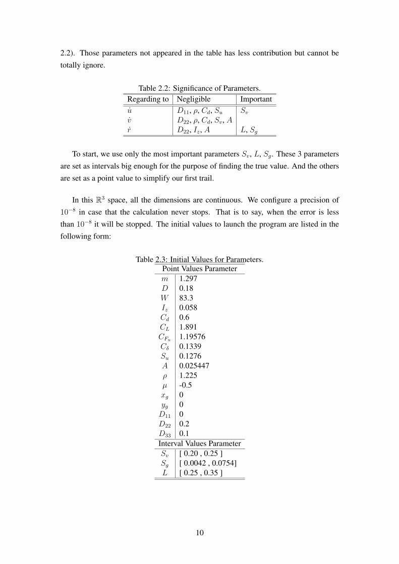
2.2). Those parameters not appeared in the table has less contribution but cannot be

totally ignore.

Table 2.2: Significance of Parameters.Regarding to Negligible Importantu D11, ρ, Cd, Su Svv D22, ρ, Cd, Sv, Ar D22, Iz, A L, Sg

To start, we use only the most important parameters Sv, L, Sg. These 3 parameters

are set as intervals big enough for the purpose of finding the true value. And the others

are set as a point value to simplify our first trail.

In this R3 space, all the dimensions are continuous. We configure a precision of

10−8 in case that the calculation never stops. That is to say, when the error is less

than 10−8 it will be stopped. The initial values to launch the program are listed in the

following form:

Table 2.3: Initial Values for Parameters.Point Values Parameterm 1.297D 0.18W 83.3Iz 0.058Cd 0.6CL 1.891CFu 1.19576Cδ 0.1339Su 0.1276A 0.025447ρ 1.225µ -0.5xg 0yg 0D11 0D22 0.2D33 0.1Interval Values ParameterSv [ 0.20 , 0.25 ]Sg [ 0.0042 , 0.0754]L [ 0.25 , 0.35 ]

10

2.4 Designed Scenarios

In real life environment, we may have different requirements for the robot. These

requirements are also different path or different mode of fly of our hovercraft. More

professionally, it is called a scenario. Here are the example of 4 different scenarios:

(a) Scenario 1 (b) Scenario 2

(c) Scenario 3 (d) Scenario 4

Figure 2.2: Example of Different Scenarios

We designed 3 scenarios:

1. The first one is a period of acceleration which allows to reach the stable speed

Vc = 2m/s in 1 second. The hovercraft follows a line in the direction of x-axis.

11

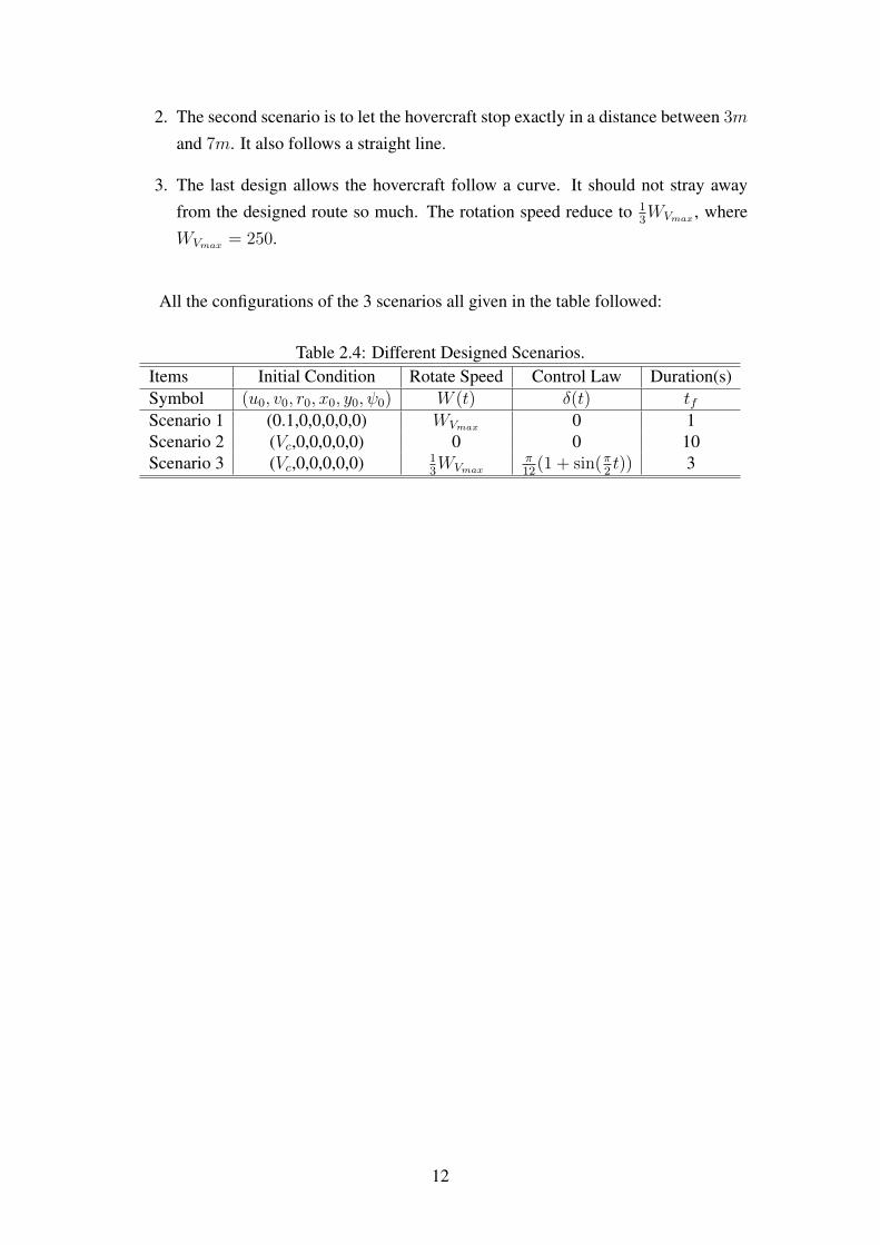
2. The second scenario is to let the hovercraft stop exactly in a distance between 3m

and 7m. It also follows a straight line.

3. The last design allows the hovercraft follow a curve. It should not stray away

from the designed route so much. The rotation speed reduce to 13WVmax , where

WVmax = 250.

All the configurations of the 3 scenarios all given in the table followed:

Table 2.4: Different Designed Scenarios.Items Initial Condition Rotate Speed Control Law Duration(s)Symbol (u0, v0, r0, x0, y0, ψ0) W (t) δ(t) tfScenario 1 (0.1,0,0,0,0,0) WVmax 0 1Scenario 2 (Vc,0,0,0,0,0) 0 0 10Scenario 3 (Vc,0,0,0,0,0) 1

3WVmax

π12(1 + sin(π

2t)) 3

12

Chapter 3: Constructed Algorithms

3.1 First Algorithm

With the aim of conduct all the selected parameters in to a interval small enough,

we make use of the method of interval analysis [9]. There is a library named Ibex

which include thousands of useful functions of interval calculation. And through the

instrumentality of DynIbex, a derivative tool from Ibex, we are able to solve initial

value problem of ordinary differential equations under interval analysis method. It will

be extremely helpful to our subject since the states equations are represented in the

derivation form and all states should be calculated by calculus.

We also apply a so-called method of bisection, to divide the purpose interval into 2

parts each time. This allows us to search in all the resolution space.

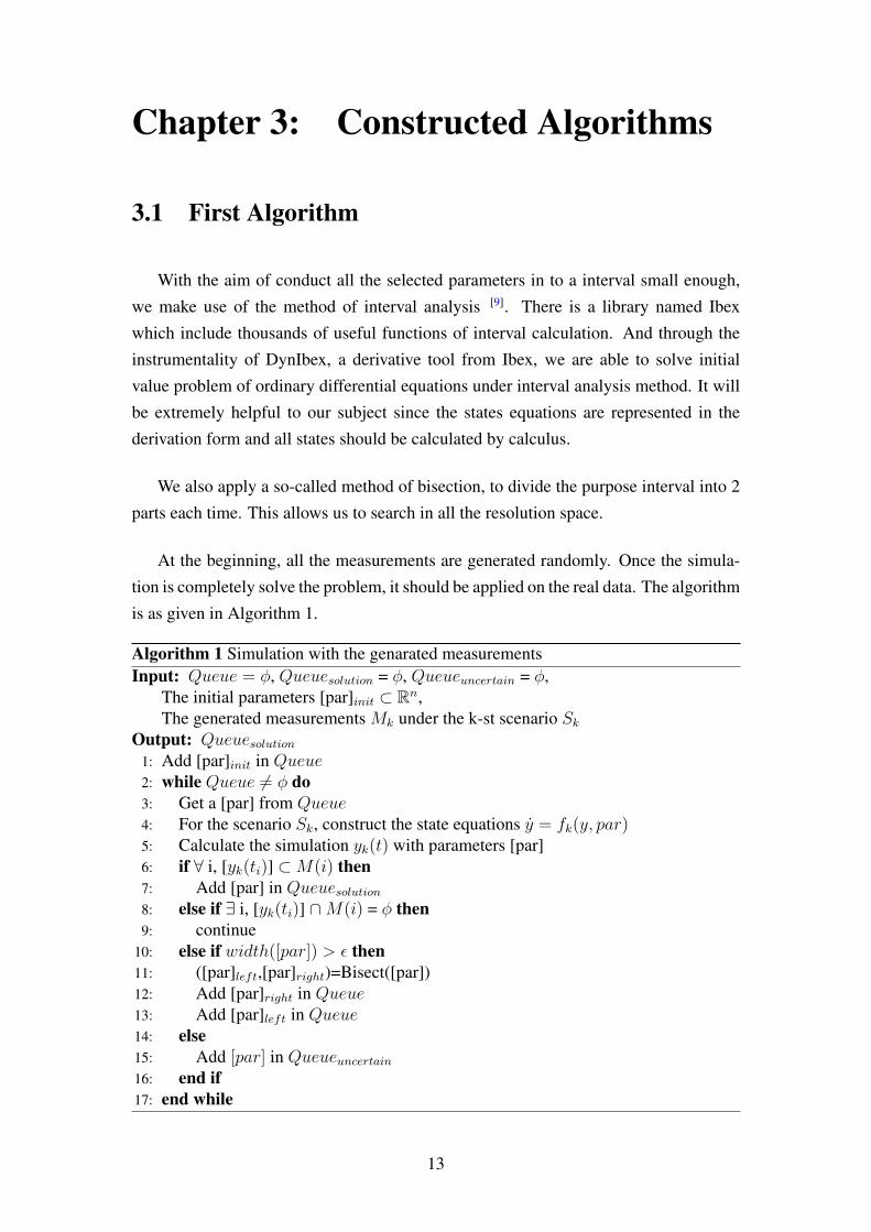
At the beginning, all the measurements are generated randomly. Once the simula-

tion is completely solve the problem, it should be applied on the real data. The algorithm

is as given in Algorithm 1.

Algorithm 1 Simulation with the genarated measurementsInput: Queue = φ, Queuesolution = φ, Queueuncertain = φ,

The initial parameters [par]init ⊂ Rn,The generated measurements Mk under the k-st scenario Sk

Output: Queuesolution1: Add [par]init in Queue2: while Queue 6= φ do3: Get a [par] from Queue4: For the scenario Sk, construct the state equations y = fk(y, par)5: Calculate the simulation yk(t) with parameters [par]6: if ∀ i, [yk(ti)] ⊂M(i) then7: Add [par] in Queuesolution8: else if ∃ i, [yk(ti)] ∩M(i) = φ then9: continue

10: else if width([par]) > ε then11: ([par]left,[par]right)=Bisect([par])12: Add [par]right in Queue13: Add [par]left in Queue14: else15: Add [par] in Queueuncertain16: end if17: end while

13

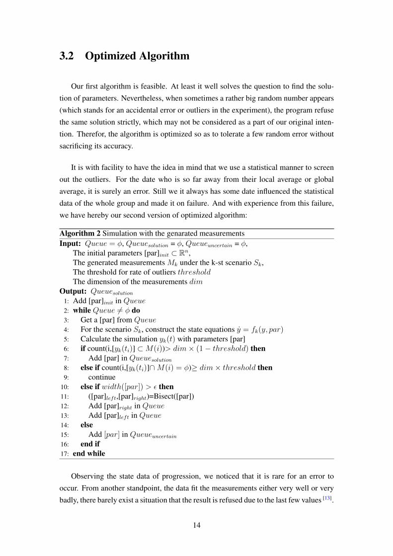
3.2 Optimized Algorithm

Our first algorithm is feasible. At least it well solves the question to find the solu-

tion of parameters. Nevertheless, when sometimes a rather big random number appears

(which stands for an accidental error or outliers in the experiment), the program refuse

the same solution strictly, which may not be considered as a part of our original inten-

tion. Therefor, the algorithm is optimized so as to tolerate a few random error without

sacrificing its accuracy.

It is with facility to have the idea in mind that we use a statistical manner to screen

out the outliers. For the date who is so far away from their local average or global

average, it is surely an error. Still we it always has some date influenced the statistical

data of the whole group and made it on failure. And with experience from this failure,

we have hereby our second version of optimized algorithm:

Algorithm 2 Simulation with the genarated measurementsInput: Queue = φ, Queuesolution = φ, Queueuncertain = φ,

The initial parameters [par]init ⊂ Rn,The generated measurements Mk under the k-st scenario Sk,The threshold for rate of outliers thresholdThe dimension of the measurements dim

Output: Queuesolution1: Add [par]init in Queue2: while Queue 6= φ do3: Get a [par] from Queue4: For the scenario Sk, construct the state equations y = fk(y, par)5: Calculate the simulation yk(t) with parameters [par]6: if count(i,[yk(ti)] ⊂M(i))> dim× (1− threshold) then7: Add [par] in Queuesolution8: else if count(i,[yk(ti)]∩M(i) = φ)≥ dim× threshold then9: continue

10: else if width([par]) > ε then11: ([par]left,[par]right)=Bisect([par])12: Add [par]right in Queue13: Add [par]left in Queue14: else15: Add [par] in Queueuncertain16: end if17: end while

Observing the state data of progression, we noticed that it is rare for an error to

occur. From another standpoint, the data fit the measurements either very well or very

badly, there barely exist a situation that the result is refused due to the last few values [13].

14

For this reason, we add a counter to each sub-program so that we can count the number

of faults that makes it refused or accepted. Then we set a threshold for error tolerance.

Taking 10% as example, if all the other 90% values passed the verification, the whole

result will be accepted.

3.3 Simulation Data Generation

To be on the safe side, our program does not begin with a real experimental envi-

ronment. All the experiments were firstly done by simulation. Hence the first step is to

generate the measurements for simulating. The procedure is as follows:

1. Define all the parameters pinit as constants with apriori experience. For the pa-

rameters to solve, make sure the value is chosen in its interval.

2. With all the parameter defined, calculate all the states for a duration tf .

3. For each state, get its real corresponding measurements [Mreal].

4. Calculate the average Mmid of the lower bound and upper bound of Mreal

5. Generate a random error ε in relation to the scale of Mreal.

6. Define a rate of interval width s.

7. Get the final generated measurements Mk = (Mmid + ε) · [1− s, 1 + s]

As we can see, Mk is also the input of our algorithm.

3.4 Real Experiment

All the word are done under simulation. The part of real experiment was not ac-

complished by me, thus will not be introduced in this report.

15

Chapter 4: Results and Conclusion

4.1 Results

The aim of algorithm validation is to confirm that it will perfectly suit the hover-

craft model and has long term application. Thereby our crucial test is on the validity.

We firstly define all the parameter and generate the measurements, then we launch the

program with the parameters hidden and tried to find them back.

We apply this methodology to the hovercraft model, and it at last carried out the

results. It find out the initial parameters successfully.

Figure 4.1: Mesuremensts well Fit the Intervals.

Here is an example shown in Figure 4.1. In order to show it more clearly and visibly,

we extract one dimension of the states in a duration of 30 seconds rather than present

all of them. We can see that there are 2 outliers in the measurements, which are added

by purpose. These outliers are so enormous that cannot be ignored at all. This may be

caused by static electricity on electric components or a wired wind. With such a group

of data, the first algorithm fails while the optimized version accept with success in all

the 3 different scenarios.

Given a error tolerance of 3 outliers, the program shows that there exists indeed a

solution to our former problem. By the result, we can also analyze the possibility of our

16

designed low of control [7].

4.2 Conclusion

In this report, we constructed a mathematical model based on an existent hovercraft.

At the very beginning, all the theoretical basic concerned are reviewed. Next, based on

the model of hovercraft, we analyzed the parameters and designed different scenarios.

Furthermore, we constructed the algorithm to solve the core problem and let it be op-

timized. At last we did some simulation experiments and verified the algorithm. The

result of this experiment is quite useful in further researches.

4.3 Acquisition

In the three months of internships, first of all, the most direct acquisition is on the

professional techniques. I did not only practiced the knowledge I got from class, such as

interval analysis, but also make me more skilled by learning a number of new expertise.

Meanwhile, working three months in a more professional environment, makes me

better and faster adapt to working life and rhythm after graduation .

In the period of internship, I understood more about the needs of company and of

our own development. Before, when someone asked me I would like to engage in what

kind of job in the future, I can not answer it precisely, or can only answered that I want

to word on IT. Now I get more recognized about myself.

4.4 Future Application

It is well-known that an accurate model is very important to improve the robot

control [14], thus a precise parameter identification contributes a lot to the development

of robotic science. As long as we get a model with very accurate parameters, we can do

all kinds of control without any difficulty. Therefore, it will be useful to such kind of

heated subject, like unmanned drive, self cruising or intelligent search.

Simultaneously, a series work of optimization should be done. Even if this algorithm

17

can solve our problem, it is too long for a dynamic environment [15]. Imagined what

happens when the drone meet a barrier and cannot get the result in 0.1 seconds. A good

optimization of time complexity will do good to the expand of model-based control, as

well as the prospect of the whole robot industry.

18

Chapter 5: Acknowledgment

There is no way to deny that it is a tremendous challenge for me to work in a

real French environment. But thanks to some people’s tireless efforts, I finished my

internship as well as this report. Without their help, I may fail thousands of times and

never had it done.

My deepest gratitude goes first and foremost to Professor Chapoutot and Doctor

Alexandre dit Sandretto, who are the supervisors in the organization of internship. Pro-

fessor Chapoutot gave me this opportunity to work in ENSTA-Paristech. He pointed

out the main direction to work and satisfied all my needs in the experiment. Doctor

Alexandre dit Sandretto gave me more concrete direction in my process of internship.

There exists his suggestion nearly in the whole procedure.

And last but not least I want thank Professor Jaulin, my tutor at school. He intro-

duced this job for me with several contacts to ENSTA-Paristech. All my knowledge of

interval analysis is learned from him.

19

Bibliography

[1] Julien Alexandre Dit Sandretto, Douglas Piccani de Souza, and Alexandre

Chapoutot. Appropriate design guided by simulation: An hovercraft application.

2016.

[2] Julien Alexandre Dit Sandretto. Etalonnage des robots a cables: identification et

qualification. PhD thesis, Universite Nice Sophia Antipolis, 2013.

[3] Jun Wu, Jinsong Wang, and Zheng You. An overview of dynamic parameter iden-

tification of robots. Robotics and computer-integrated manufacturing, 26(5):414–

419, 2010.

[4] Wisama Khalil, Etienne Dombre, and ML Nagurka. Modeling, identification and

control of robots. Applied Mechanics Reviews, 56:37, 2003.

[5] Vassilios D Tourassis and Charles P Neuman. The inertial characteristics of dy-

namic robot models. Mechanism and machine theory, 20(1):41–52, 1985.

[6] Sylvain Guegan, Wisama Khalil, and Philippe Lemoine. Identification of the dy-

namic parameters of the orthoglide. In Robotics and Automation, 2003. Proceed-

ings. ICRA’03. IEEE International Conference on, volume 3, pages 3272–3277.

IEEE, 2003.

[7] Luc Jaulin. La robotique mobile. ISTE, 2015.

[8] Pradeep K Khosla and Takeo Kanade. Parameter identification of robot dynamics.

In Decision and Control, 1985 24th IEEE Conference on, pages 1754–1760. IEEE,

1985.

[9] Hou Yangyi and Fang Hairong. Application of interval analysis theory in robot

dynamics parameter identification. Mechanics, 35(4):64–66, 2008.

[10] Luc Jaulin. Applied interval analysis: with examples in parameter and state es-

timation, robust control and robotics, volume 1. Springer Science & Business

Media, 2001.

[11] Matthew D Stuber and Paul I Barton. Robust simulation and design using para-

metric interval methods. In 4th International Workshop on Reliable Engineering

Computing (REC 2010), pages 536–553. Citeseer, 2010.

[12] J Alexandre dit Sandretto and Alexandre Chapoutot. Validated explicit and im-

plicit runge-kutta methods. Reliable Computing, 22:79, 2016.

20

[13] Andres Vivas, Philippe Poignet, Frederic Marquet, Francois Pierrot, and Maxime

Gautier. Experimental dynamic identification of a fully parallel robot. In Robotics

and Automation, 2003. Proceedings. ICRA’03. IEEE International Conference on,

volume 3, pages 3278–3283. IEEE, 2003.

[14] Stephen M Batill, John E Renaud, and Xiaoyu Gu. Modeling and simulation

uncertainty in multidisciplinary design optimization. AIAA paper, 4803, 2000.

[15] R Serban and JS Freeman. Identification and identifiability of unknown parame-

ters in multibody dynamic systems. Multibody System Dynamics, 5(4):335–350,

2001.

21