1

Abstract—The image of secondary arc, which is a common phenomenon in ultra high voltage (UHV) power system, contains a wealthy of information. To determine its geometrical characteristics, the secondary arc image is systematically processed involving gray scale, noise filtering, image segmentation, etc. To overcome the discontinuous and false edge caused by conventional operators, an improved algorithm is employed; the unrelated edges are fully removed, and the interrupted endpoints are dilated. Based on the results, the component and evolution of secondary arc are discussed; the correlation of the arc luminance and arc current is revealed. Occasionally, the arc roots and arc column have irregular motion behaviour. Using the edge-detection technique, the detailed jumping location and velocity of anode arc root are tracked; the life expectancy and stability of coexistence of multi cathode arc roots are determined; the morphology of short circuit of arc column is ascertained. Furthermore, the secondary arc dimension is estimated in our work, including the arc radius and arc length. A number of formulas have been presented to predict the dimension. The obtained results are more accuracy than previous works.

Index Terms—Secondary arc; Edge detection; Laplacian operator; Irregular arc motion; Secondary arc dimension

I. INTRODUCTION ingle phase auto-reclosing scheme is widely used in high voltage transmission lines. When a fault occurs on a transmission line, the phase would be isolated from both

ends by the related protective relays. In this condition, some voltage is induced on the isolated phase due to capacitive and inductive couplings among the healthy and faulted phases [1]. The induced voltage feeds current through the fault point causing arc consistency, forming the so-called secondary arc. The secondary arc is burned in the ionized, hot plasma channel along the insulator string, and it is a common phenomenon of high voltage power systems, especially with voltage above 500 kV. The secondary arc is essentially a small current AC electric arc, which consists of electrons, positive ions and neutral molecules [2],.Depending on the line parameters, its current ranges from several to tens of amperes. Its arcing process is closely related to the protection scheme, and has a strong impact on the operation of the system. To fulfill the transient stability criteria, the extinction time of secondary arc should be limited to be less than 1 s [3].

Extensive research has been conducted on the subject of secondary arc, covering the electromagnetic transients, the arc physics and the suppressing techniques. A. T. John et al [4] developed a time-dependent model; the interaction between the secondary arc and the system was investigated in detail. A series of non-confined secondary arc tests were conducted on 500 kV real towers, and the harmonic content of secondary arc voltage were researched [5]; a 3D snake-based approach was pretended to reconstruct the arc shape. T. Tsuboi reported the field data on secondary arc recorded during lightning fault,

and a number of equations were proposed to compute the extinction time [6]. The motion of secondary arc is a hot topic, and fascinated by engineers. Considering the electromagnetic force, the resistive force, the wind effect and the thermal buoyancy, the mechanical model of secondary arc were developed [7].

The image is a straightforward method for secondary arc study. It is a set of digital data in essence and includes a wealthy of valuable geometrical information, e.g., location, dimension as well as moving velocity [8]. Although substantial secondary arc trajectories have been obtained during tests, the quality of most captured images is relatively poor, which poses a challenge for the in-depth elucidation of secondary arc physics. For instance, as the secondary arc temperature is extremely high, ranging from thousands to tens of thousands centigrade [9], which exceed the boiling point of copper, and the electrode is inevitably vaporized, affecting the identification of true arc body; the arcing process is often accompanied by strong light, leading to the saturation of optical sensors; the light emitted from arc column normally weaken luminous arc roots; in addition, due to the electromagnetic interferences, the secondary arc image are sometimes corrupted by noises.

The image processing technology has been developed for decades and recently it has been applied to arc plasma study. In Ref. [10], the dual-jet DC arc plasma images are grayscaled and binarily segmented. Based on the spectroscopic line-ratio method at two specified wavelengths, the temperature of the arc is obtained; in Ref. [11], the image processing technique is employ to process real-time JET video for the purposing of identifying moving object. To visualize the arc splashing erosion, the centroid coordinates and the boundaries of droplets are detected via a 5×5 Laplacian mask in [12]. The edge detection is a key and fundamental step in image processing [13]. Generally, the edge indicates an abrupt change or a discontinuity in gray levels of an image, and it is equal to abstracting the high-frequency components. A number of operators have been proposed, like Sobel operator, Laplacian operator [12], Canny operator and so on [14]. The performances of these operators are highly dependent on the given case, and they have certain limitations, e.g., sensitive to noise and may fail at some corners. Few general agreements have been achieved yet, and more importantly the detected edges are often fragmented, discontinuous and even false [15].

In this work, the geometrical characteristics of secondary arc are investigated using a novel edge detection technique. The main contribution and the structure of this work are outlined as follows.

To obtain secondary arc image, an experiment is setup and a series of experiments have been performed, as presented in Section II.

The principle of image processing, involving grayscale,

Investigation on the Geometrical Characteristics of Secondary Arc by Image Edge Detection

Q. Sun, Member, IEEE, F. Liang, F. Wang, H. Cong, Q. Li, and J. Yan

S

2

filtering, segmentation and edge detection, is then described in Section III.

Section IV is devoted to the evolution of secondary arc. Using edge detection, its characteristics are discussed.

In Section V, the irregular secondary arc motion behavior is identified, and its dimension is estimated.

Finally, the conclusion is addressed in Section VI.

II. EXPERIMENT SETUP A. Topology of Main Circuit

To investigate the characteristics of secondary arc, a series of experiments have been performed at High-Power Laboratory of CEPRI. The experimental setup consists of a main circuit, a voltage divider (VD) and a current transformer (CT). An arcing horn, as depicted in Fig. 1, is installed in parallel with the insulator for guiding the electric arc. The gap between the upper electrode and the lower electrode are adjusted, depending on the insulator string. The dimension of the insulator string as well as the arcing horn is listed in Table I [7]. In order to ignite the arc, the insulator string is shorten by a nitrogen fuse (Φ=0.15 mm, nickel). The voltage and current of secondary arc are measured by VD and CT, respectively, and then input into the digital oscilloscope (Yokogawa, DL850) with a sampling rate of 1GS/s. The data are eventually transferred to the computer via a GPIB interface for further analysis. A high-speed CCD-based camera (Motion Pro X3) is employed to capture the arc trajectories.

High speed camera

ComputerDigital Oscilloscope

Insulator string

Upper electrode

Fuse wire

Lower electrode

Reactor

Capacitor

S1

S2

CT

VD

GPIB

Powersource

(a)

0Z

Z1

Zc

Zp

Xc

Xd

X

Y

Current

Current

Arc column

Motion direction

Anode arc root

B

Cathode arc root

Electrode

Electrode

(b) Fig. 1. Experiment setup. (a) Schematic diagram of the main circuit. (b) Structure of arcing horn.

TABLE I DIMENSION OF INSULATOR STRING

Xc Xd Zc Zp Z0 Z1

0.32 m 0.14 m 0.17 m 0.17 m 0.68 m 1.02 m

The circuit breakers are controlled by a programmable logic controller, and the operating sequence is depicted in Fig. 2. Firstly, the circuit breaker S1 is switched on at t1, and a high current (primary arc) would flow through the fuse, igniting the primary arc. After an interval of t1, a switching off signal and ∆a switching on signal would be sent to S1 and S2, respectively. After a time delay (including the relaying time, the operating time and arcing time), the primary arc would be extinguished, followed by the initiation of secondary arc. Depending on the inductance L and the capacitance C, the magnitude of secondary arc ranges from tens to hundreds of amperes. Once the secondary arc is extinguished, all the circuit breakers would be switched off, and the experiment is completed.

Primary arc

Switching on, S1

CB

ope

ratio

nA

rc ty

pe

Switching on, S2

Initiation

Secondary arc

Finish

1t2t

Switching off, S2

Extinction

Arc

cur

rent

Switching off, S1

Start

Fig. 2. Operating sequence of circuit breakers.

B. Image Sensing System The high-speed camera is a key component in the

experiments. The performance of the imaging system is mainly controlled by three parameters, i.e., the focal length,

H h

u v

Dfc

Lens

Fig. 3. Imaging principle of high speed camera. the aperture and the frames. The principle of the imaging system is illustrated in Fig. 3.

The focal length of camera is defined as (1) 𝑓C = 𝑣

𝑢𝐻

where is the distance between the sensor and the lens, 𝑣 𝑢is the distance between the object and the lens, and 𝐻represents the height of the target object. Since H ranges from 0.5 to 1.0 m, and is about 5.0 m, is set to be 80 mm in our 𝑢 𝑓Cexperiment.

The aperture determines the cone angle of rays. The amount of light captured by lens is proportional to the area of the aperture,

3

(2) 𝑅 =1.22𝜆𝑓

𝐷 = 1.22𝜆𝐹where R is the radius of diffraction spot, λ is the wave

length of incident light, D is the size of the aperture, and F represents the relative size of the lens aperture. Clearly, the size of diffraction spot is directly proportion to F. To guarantee the image resolution, F is set to be 1.4 and the exposure time is set to be 2 ms. In order to reduce the strong light, an optical filter with band pass of 320 nm - 480 nm is placed in front of the lens. Since the arcing time is around several seconds, the maximum resolution and frames per second are set to be 796×992 and 500, respectively. Hence, the imaging time of the device is as high as one minute, which enables us to obtain the entire evolution of discharges.

III. PRINCIPLES OF IMAGE PROCESSING The operations performed in image processing involve three

major stages, i.e., preprocessing, basic edge detection and removing unrelated edge points. The flowchart is illustrated in Fig. 4.

Are all the Pixels from the basic

edges removed

End

Grayscale

Start

Noise Filtering

Segmentation

Use Lapalacian operator to detect basic edges

Output the longest edge from the temporary image

Compute the maximum length of

any two points

Get the temporary edge

Select one of the conjunction points and

set it as the search center

Search from one of the neighbors, and set other

neighbors as unprocessed conjunction points

Check the conjunction point

Find one end point

Select any point from the edges as a search center

Remove this point

Neighbor number of search center=0?

Find the neighbors of the search center

Neighbor number of search center=1?

Neighbor number of search center=1?

Preprocessing

Basic edge detection

Removing unrelated points

Fig .4. Flowchart of secondary arc image processing.

Step 1) Grayscale of Image Consider a digital image having L gray levels, and let Y be

the luminance at pixel coordinate [i, j], (0≤ i, j≤L-1), as represented in Fig. 5 [16].

i

j

Y(i, j)

Fig. 5. 3×3 neighborhood. Since the majority of original images captured from camera

are in RGB format, the image is required to be gray scaled. The luminance, denoted by Y, is essentially a weighted sum of red (R), green (G) and blue (B) colors. The weighting coefficients are proportional to the perceptual response to each component. Mathematically, the luminance of each pixel can be expressed as

Y(i, j) = 0.2989R(i, j)+0.5870G(i, j)+0.1140B(i, j) (3) Step 2) Noise filtering

The second step is to filter out noises. To prevent edge blurring and loss of image details, the median filter is applied [17].

(4) 𝑓(𝑖,𝑗) =1𝑀∑

(𝑚,𝑛) ∈ 𝑆∑𝑙(𝑚,𝑛)𝑌(𝑖 ‒ 𝑚,𝑗 ‒ 𝑛)

where is the output vector, l is the 3×3 convoluting 𝑓(𝑖,𝑗)mask, S is the chosen area, M is the amount of the neighboring pixels, and it is equal to 8 for our case.

Step 3) Image segmentation The arc body has a stronger luminance in comparison to the background. To facilitate the analysis, the filtered image is grouped and segmented into a binary one. This operation can be expressed as

(5) {𝑓(𝑖,𝑗) = 1 𝑓(𝑖,𝑗) ≥ 𝑇𝑓(𝑖,𝑗) = 0 𝑓(𝑖,𝑗) < 𝑇�

where T is the threshold. The determination of this value is a key step for the operation. The Otsu's method is employed in our work. This algorithm assumes that the image contains two classes of pixels following bi-modal histogram; it has exhibits good performance if the histogram can be assumed to have bimodal distribution and assumed to possess a deep and sharp valley between two peaks. Threshold values from image to image vary since the variations in the gray values in the neighbourhoods of pixels vary from image to image [18, 19]. The Otsu's method exhaustively searches for the threshold that minimizes the intra-class variance given in Eq. (6).

(6) 𝜎2𝜔(𝑇) = 𝜔0(𝑇)𝜎2

0(𝑇) + 𝜔1𝜎21(𝑇)

where are the probabilities of the two classes separated 𝜔0,1

by a threshold T and are variances of these two classes. 𝜎 20,1

The class probabilities are computed from the L 𝜔0,1(𝑇)histograms:

4

(7) {𝜔0(𝑇) = ∑𝑡 ‒ 1

𝑖 = 0𝑝𝑖

𝜔1(𝑇) = ∑𝐿 ‒ 1

𝑖 = 𝑡𝑝𝑖�

Step 4) Using Laplacian operator for detecting basic edges Taking advantages of the simplicity, the Laplacian operator

is performed to measure the basic spatial gradient and orientation of the image, as given in Eq. (8)

(8) ∇2𝑓(𝑥,𝑦) = [𝐺𝑥𝐺𝑦] = [∂2𝑓

∂𝑥2

∂2𝑓

∂𝑦2]

The magnitude and angle of the vector are given by

(9) {mag (∇2𝑓) = (∂2𝑓

∂𝑥2)2

+ (∂2𝑓

∂𝑦2)2

𝛼 = tan ‒ 1 (𝐺𝑦

𝐺𝑥) �

This mask of Laplacian operator is illustrated in Fig. 6.

-1/8-1/8-1/8

-1/8-1/8-1/8

-1/81-1/8

1/81/81/8

1/81/81/8

1/801/8

000

000

010= -

All-pass filter Round mean filterLaplacian operator

Fig. 6. Mask of Laplacian operator; (a) a mask of a round mean filter; (b) a mask of a all-pass filter.

It consists of two parts, i.e., a round mean filter and an all-pass filter. The former compute edge information whistle the latter estimate the local mean. By means of a subtraction operation, the local high-frequency components are then obtained. The edge detection is determined by the gradient of luminance variation rather than the luminance value itself [20, 21]. As a consequence, the result is insensitive to the camera setting.

Step 5) Removing unrelated edges The detected edges are sometimes discontinuous and false.

In this step, we will search all points of basic edges and remove unrelated ones. The details are depicted in Fig. 4 [22].

Select any point from basic edges as a center, and search a 3×3 neighboring area. Depending on the neighbor number, three cases are considered:

Case i) if there is no neighboring pixel, the selected point is an isolated one and would be directly removed;

Case ii) if there is only one neighbor, the selected point is set as an end point;

Case iii) if the neighbor number is larger than one, the point is a normal transition one. Set one of the neighboring pixels as a new center, and start a new search. Store other pixels as unchecked conjunction points.

Check the conjunction points. If all of them have been searched as a center, one temporary edge is obtained.

Step 6) Determination of defined edges Compute the length of any two endpoints, and output the

longest one as the true edge.

IV. RESULTS AND DISCUSSION A. Results

More than 100 sets of images have been acquired during the experiments. Figure 7 illustrates a representative evolution of secondary arc in one cycle. To focus on the entity under study, only the main arc body is presented.

(a)

t=0.120 0.122 0.124 0.126 0.128 0.130 0.132 0.134 0.136 0.138s

(b)

Fig.7. Evolution of secondary arc in one cycle. From Fig. 7 (a), it can be observed that both the voltage and

current are greatly distorted due to the nonlinear variation of secondary arc. The waveforms contain considerable harmonics, and through the Fourier analysis, it shows that the RMS of the current and voltage are 30 A and 4 kV, respectively. The voltage waveform slightly leads the current one. As the current crosses zero, the secondary arc would experience the so-called zero-crossing period, the duration of which is about a number of milliseconds. The presence of active elements, i.e. the capacitor and inductor, would give rise to the transient processes, and the waveform fluctuates. The movement of secondary arc is not independent. It is physically controlled by the voltage and current, in other words, the electromagnetic transient of the system. Such fluctuation can be served as an indicator of the smoothness of arc movement. The secondary arc is resistive in nature. It is a passive circuit element from the perspective of electric circuit, and cannot storage the energy. The voltage-current curve would shape in the same quadrant of coordinate system. The zero crossings for the current and the voltage would occur at the same moment.

The current through the electrode and the arc body itself creates a strong magnetic field [23-27]. On one hand, the arc roots bear a higher magnetic force, and they climbs more rapidly along the electrode [27]. The arc roots keep ahead of the arc column, and the latter is drawn by the former. On the other hand, the rotational magnetic force makes the arc column continuously rotate, and the secondary arc periodically swings. Once the cathode and anode arc roots are driven to the terminal of electrodes, the roots are fixed, and the mean

5

velocity of the arc roots becomes zero. The arc column, however, is still moving. Due to the variations in operating environment, the arc length, the magnetic field as well as the forces on arc body, etc., the motion characteristics of secondary arc is slightly different from that of the switching arc operated in a closed chamber [26].

The arc is subject to the wind force, the resistive force, the thermal buoyancy and the Lorenz force [7]. Under the small wind condition and the secondary arc reaches the steady state, the magnetic force stressed on the arc column can be considered to be equal to the resistive force.

(10) {𝐹𝑟 =12𝐶ρ𝑑𝑙ν2

𝐹𝑚 = 𝐼𝑙𝐵 �Therefore,

(11) ν ≈2IBCρd

where v is the mean speed, is the density of air and C is ρa constant, d is the secondary arc diameter, l is the secondary arc length. As the wind velocity and temperature increases, the wind force plus the resistive force may overtake the magnetic force, and the velocity of arc become quite small [7]. Momentarily, the arc roots have immobility. Under certain conditions, it even moves in the opposite direction. Since the discharge is severe, the evolution of secondary arc is accompanied by large audible noises and many sparks.

Regarding the secondary arc image, from a microscopic point of view, the brightness of electric arc evidences the photons produced during the ionizing and recombination processes. Since I=JA=nqvA and J=σ/E, the conductivity is directly proportional to the current density. The increases in the current enable more plasmas and electron energy to be expended. Hence, the luminance of the image closely correlates with the current, and it periodically changes. As the current rises, the image becomes more luminous; as the current passes through zero, it becomes relatively dark. The discharge voltage is jointly determined by the arc current and arc length [4], and the luminance intensity has a weak relationship with it. Some regions of the images are clear. However, the boundary area is too blurry to extract the shape and track the position of pixel directly. The image quality is governed by thermal effect rather than the plasma effect (the ionization and the energy transport process, etc.). B. Discussion

Fig. 8 gives an example of secondary arc image with 796×992 pixels. The spatial resolution, denoted by ε, was 1 pixel for 1.13 mm. The images are input into MATLAB and implemented using the aforementioned algorithm.

(a)

(b)

(c)

Fig. 8. Luminance of secondary arc image. (a) original image (b) Luminance histogram. (c) luminance along specified line.

The image is composed of three areas, i.e., the background, the boundary area and the arc body. The arc body consists of the anode arc root, the arc column and the cathode arc root. The image histogram, which reflects the relative frequency of occurrence of each pixel values, is given in Fig. 8 (b). It indicates that the pixel intensities of the image are non-uniformly distributed. The peaks in the lower range correspond to the background whereas those in the higher range correspond to the arc body. The value of pure dark area is zero. The center of arc column reaches the maximum, and the intensity decreases from the central to the outside.

Background

Arc column

Boundary

Cathode arc root

Anode arc root

10 cm

Specified line

6

(a) (b)

(c) (d)

Fig. 9. Processing of secondary arc image. (a) Image filtering. (b) Image segmentation. (c) Basic edge detection using Laplacian operator. (d) Removing unrelated edges.

The image is grayscaled, and by applying the mean filter over a window of 3×3 for each pixel, most of the noises have been removed, as shown in Fig. 9 (a). The blurry area becomes sharp while the details are preserved. As a result of binary segmentation, the image has been logically divided into two sorts, i.e., zero and one. The background is distinguished from the arc body. Using the Laplacian operator, the zero crossings of the image are finally obtained and the basic profile is detected, including many local edges invisible. It shows that the edge extracted from this nontrivial image is mixed by fragmentation. Several basic edge curves are not connected, and edge segments are melted. A part of the boundary area is wrongly identified which are obviously not the real edge of the main arc body. Comparatively, using the algorithm presented in this work, the unrelated endpoints have been removed. Only one clear, continuous, and uninterrupted edge is obtained. The noise, reflection and edge blurry are resolved. Due to the involvement of step 5 and 6, the running time is not as fast as existing operators, at the price for obtaining a better performance. It spends 832 ms to process this image on a 2.40 GHz Intel Core i5-4258U CPU-based personal computer.

V. APPLICATION OF EDGE DETECTION TO SECONDARY ARC STUDY

The arc roots and arc column have different motion characteristics [28-31]. The edge-detection technique can aid

the identification of the behaviors and the exact estimation of secondary arc dimension. A. Identification of Irregular Arc Motion Behavior

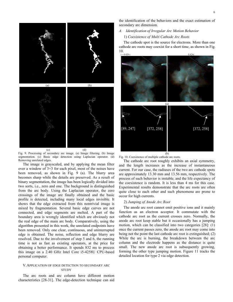
1) Coexistence of Multi Cathode Arc Roots The cathode spot is the source for electrons. More than one

cathode arc roots may coexist for a short time, as shown in Fig. 10. t = 0.420 s 0.424s

(a)

(b)

Fig. 10. Coexistence of multiple cathode arc roots. The cathode arc root roughly exhibits an axial symmetry,

and the length increases as the increase of instantaneous current. For our case, the radiuses of the two arc cathode spots are approximately 13.30 mm and 13.56 mm, respectively. The process of such behavior is instable, and the life expectancy of the coexistence is random. It is less than 4 ms for this case. Experimental results demonstrate that the arc roots are often quite close to each other and such phenomena are prone to occur for high currents.

2) Jumping of Anode Arc Root The anode arc root cannot emit positive ions and it mainly

function as an electron acceptor. It commutate with the cathode arc root as the current crosses zero. Normally, the anode arc root keep stable but it occasionally has a jumping motion, which can be classified into two categories [28]: (1) once the current passes zero, the anode arc root may come into being not the point the last cathode arc root is extinguished; (2) While the arc is burning, the breakdown between the arc column and the electrode happens as the distance is quite small. The new anode arc root is subsequently growing, forming the other type jumping motion. Figure 11 tracks the detailed location for type 2 via edge detection.

[89, 247] [372, 258] [372, 258]

7

t= 0.128s 0.132s

(a)

(b)

Fig. 11. Identification of the jumping of anode arc root. The distance before this jump is around 30.10 mm in our

case. Since the time interval is 4 ms, the speed is at least 7.53 m/s.

3) Short Circuit of Arc Column The shape of secondary arc column is complex and its

length far exceeds the insulator string in parallel. The short circuit often occurs between different segments of arc column. Figure 12 presents an example of such phenomenon.

t = 0.184 0.188s

(a)

(b)

Fig. 12. Short circuit of arc column. The behavior occurs as two segments move close to each

other, and a loop is formed at t=0.188s, around the image coordinate [368, 350]. As time goes, the original column gradually disappears, and the new column becomes the

dominant one. Resulting from the decrease in arc length as well as arc resistance, the arc voltage also drops slightly. It indicates that the longer the secondary arc, the larger probability the short circuit. B. Estimation of Secondary Arc Dimension

1) Secondary arc radius The radius is a crucial factor in the heat dissipation and

motion modelling of secondary arc. Through image processing, the edge coordinates can be easily determined. Supposing [ , 𝑥𝑖_1

] and [ , ] are the coordinates of the edge points, the 𝑦𝑗_1 𝑥𝑖_2 𝑦𝑗_2secondary arc radius r is given in Eq. (12).

(12) 𝑟 =𝜀 (𝑥𝑖_1 ‒ 𝑥𝑖_2)2 + (𝑦𝑖_1 ‒ 𝑦𝑖_2)2

2where is the length of each pixel side. Table II lists the 𝜀

edge points chosen from two cases of current 30 A and 45 A, respectively. It can be observed that the radius is closely related to the motion process. Since the wind is uneven along the arc body, the content of ions diffused into surrounding air is unequal. As a consequence, the radius is slightly different along the entire arc body. Due to the branch of anode arc root caused by jumping motion [28], along with the diffusion effect of particles [31], the radius of cathode arc root is relatively larger that of others. Using curve fitting technique, the average arc radius can be derived,

(13) 𝑟 = 𝑘𝐼𝛼

where k=2.21 and α=0.47. Obviously, the increase of current would lead to higher plasma density, electron energy as well as arc radius. A number of formulas have been proposed to evaluate this quantity with respect to common arc [2], [32]. Compared with those located in closed area, the secondary arc is nearly independent of gas pressure, and the radius is relatively larger, which can be attributed to its open operating regime. In practice, given the arc radius, the quantities, like the area of cross section, the voltage drop and the moving velocity, can be further deduced [33].

2) Secondary arc length The length is often used as a criterion to evaluate the

extinction time of secondary arc. Previously, this quantity is roughly estimated through visual inspection [34]. Using the proposed method, it can be exactly determined.

After the edge detection, the image is composed of two sorts of values, i.e., 0 and 1. Clearly, 0 represents the background whereas 1 represents the edge. It can be deduced that the secondary arc length is approximately equal to half that of the edge. Mathematically,

{𝑁 =𝑚

∑𝑖 = 1

𝑛

∑𝑗 = 1

𝑓(𝑖,𝑗)

𝑙 ≈𝜀𝑁2

� (14)

Table III gives a case of current 30 A . It can be observed that: the secondary arc length is flexible and constantly changing during the motion process. Using curve fitting technique, the variation of secondary arc length can be expressed as,

𝑙(𝑡)/𝑙0 = {2.61𝑡 + 1.02 for 𝑡 < 0.10 s 0.016𝑒20.2𝑡 + 1.05 for 𝑡 ≥ 0.10 s � (15)

where is the initial value. The evolution of secondary arc 𝑙0

[334, 251] [363, 263]

[368, 250]

44. 84 mm mm

8

can be roughly divided into two stages: for the first stage, the arc column is relatively stabilized and the arc axis is parallel to the centre axis of insulator string; the secondary arc column is elongated linearly and the length is a linear function of arcing time. For the second stage, the arc column is split into a number of series segments. The moving velocity is quite high and the direction of each segment is random. As a result, the secondary arc length rises exponentially. The arc length approaches its longest before the extinction, and it is approximately twice the initial value.

As the secondary arc length is increased, more heat, would be dissipated from arc body toward surrounding area;

meanwhile, more free electrons would be diffused into the peripheral area of the arc column and collide with the cold neutral particles. These electrons would combine with the neutral particles and accelerate the de-ionizing process, which ultimately results in secondary arc extinction.

Note that the secondary arc length is significantly affected by wind. The higher the wind velocity, the longer the arc length. In our case, the velocity of the natural wind is lower than 1m/s, and the secondary arc length is relatively short. In practice, however, the insulator string line is installed at a height larger than 20 meters. As a consequence, the length may be much larger and it would benefit the extinction.

TABLE II RADIUS OF SECONDARY ARC

Current Arc Body Edge Coordinate 1 Edge Coordinate 2 Arc Radius

(mm) Average

(mm) Standard Deviation

[417 230] [429 230] 13.56 Cathode arc root

[431 194] [448 194] 19.21 [379 326] [386 326] 7.91 [426 486] [434 486] 9.04 [457 529] [466 529] 10.17

Arc Column

[487 705] [493 705] 6.78 [463 747] [472 747] 10.17

Case 1 (30A)

Anode arc root [421 832] [430 832] 10.17

10.87 3.91

[415 220] [428 220] 14.69 Cathode arc root [411 151] [428 151] 19.21

[294 213] [305 213] 12.43 [244 295] [257 295] 14.69 [433 458] [433 448] 11.30

Arc Column

[467 632] [477 632] 11.30 [430 667] [440 667] 11.30

Case 2 (45A)

Anode arc root [427 807] [436 807] 10.17

13.14 2.96

TABLE III LENGTH OF SECONDARY ARC

Stage Time instant Amount of Zero Amount of One Arc length

(cm) Initiation t = 0.00 s 800197 2619 148

t = 0.02 s 800144 2972 151 t = 0.04 s 799948 2868 162 t = 0.06 s 799630 3186 180 t = 0.08 s 799594 3222 182 t = 0.10 s 799647 3169 179 t = 0.12 s 799789 3027 171 t = 0.14 s 799293 3523 199 t = 0.16 s 798992 3824 216 t = 0.18 s 798262 4554 230

Extinction t = 0.196 s 796994 5822 294

VI. CONCLUSIONS In this work, the geometrical characteristics of secondary

arc are systematically studied. A series of experiments have been performed and hundreds sets of secondary arc images are obtained. To overcome the discontinuous and false edge caused by conventional edge detection operators, an improved algorithm is proposed; the unrelated fragmented edges are fully removed, and the interrupted endpoints are dilated. By means of edge detection, the detailed jumping location and

velocity of anode arc root are tracked; the life expectancy and stability of coexistence of multi cathode arc roots are determined; the morphology of short circuit of arc column is ascertained. Furthermore, the secondary arc radius, length as well as the area is quantitatively analyzed by processing the obtained edge coordinates, the formulas estimating secondary arc dimension are presented through curve fitting. The methodology presented in this work not only helps further understand the physical mechanism of secondary arc discharge, but also lays a basis for evaluating the arcing time.

9

REFERENCES [1] IEEE Power system relaying committee working group, “Single phase

tripping and auto reclosing of transmission lines,” IEEE Trans. Power Del., vol. 7, no.1, pp. 182-192, Jan. 1992.

[2] H. X. Cong, Q. M. Li, J. Y. Xing, and W. H. Siew, “Modeling study of the secondary arc with stochastic initial positions caused by the primary arc,” IEEE Trans. Plasma Sci., vol. 43, no. 6, pp. 2046–2053, Jun. 2015.

[3] I. M. Dudurych, T. J. Gallagher, and Rosolowski, “Arc effect on single-phase reclosing time of a UHV power transmission line,” IEEE Trans. Power Del., vol. 19, no. 2, pp. 8540-860, Apr. 2004.

[4] A. T. John, R. K. Aggarwal, and Y. H. Song, “Improved techniques for modelling fault arcs an faulted EHV transmission systems,” Proc. Inst. Elect. Eng., Gen., Trans. Distrib., vol. 141, no. 2, pp. 148-154, Mar. 1994.

[5] M. C. Tavares, J. Talaisys, and A. Camara, “Voltage harmonic content of long artificially generated electrical arc in out-door experiment at 500 kV towers,” IEEE Trans. Dielectr. Electr. Insul., vol. 21, no. 3, pp. 1005–1014, Jun. 2014.

[6] T. Tsuboi, J. Takami, S. Okabe, K. Aoki, and Y. Yamagata, “Study on a field data of secondary arc extinction time for large-sized transmission lines,” IEEE Trans. Dielectr. Electr. Insul., vol. 20, no. 6, pp. 2277–2286, Dec. 2013.

[7] Q. M. Li, H. X. Cong, Q. Q. Sun, J. Y. Xing, and Q. Chen, “Characteristics of secondary ac arc column motion near power transmission-line insulator string,” IEEE Trans. Power Del., vol. 29, no. 5, pp. 2324-2331, Oct. 2014.

[8] C. Solomon and T. Breckon, Fundamentals of digital image processing, John Wily, 2011.

[9] X. Yan, W. Chen, Z. He, et al. Temperature measurement of air arc in long gap by spectrum diagnosis, Proceedings of CSEE, vol. 31, no. 19, pp. 146-152, Jul. 2011.

[10] H. Guo, P. Li, H. Li, et al. "In situ measurement of the two-dimensional temperature field of a dual-jet direct-current arc plasma", Rev. Sci. Instrum., 87, 033502, 2016.

[11] M. de Albuquerque, M. De Albuquerque, G. T. Chacon, et al., "High-speed image processing algorithms for real-time detection of MARFEs on JET", IEEE Trans. Plasma Sci., vol. 40, no. 12, pp. 3485-3492, Dec. 2012.

[12] Yi Wu, Yufei Cui, Mingzhe Rong, et al, "Visualization and mechanisms of splashing erosion of electrodes in a DC air arc", J. Phys. D: Appl. Phys., 50, 2017

[13] D. Marr and E.C. Hildreth, “Theory of Edge Detection,” Proc. Royal Soc. London B, vol. 207, pp. 187-217, 1980.

[14] S. Konishi, A.L. Yulle, J.M. Coughlan, and S.C. Zhu, “Statistical Edge Detection: Learning and Evaluating Edge Cues,” IEEE Trans. Pattern Anal. Mach. Intell., vol. 25, no. 1, pp. 57-74, Jan. 2003.

[15] X. Wang, "Laplacian operator-based edge detectors," IEEE Trans. Pattern Anal. Mach. Intell., vol. 29, no. 5, pp. 886-890, May 2007.

[16] F. Russo, “An image enhancement technique combining sharpening and noise reduction,” IEEE Trans. Instrum. Meas., vol. 51, no. 4, pp. 824–1085, Aug. 2002.

[17] K. He, S. Jian, and X. Tang, “Guided image filtering,” IEEE Trans. Pattern Anal. Mach. Intell. vol. 35, no. 6, pp. 1397–1409, Jun. 2013.

[18] Otsu, N. “A threshold selection method from gray-level histograms,” IEEE Trans. Syst., Man, and Cyb., vol. 9, no. 1, pp. 62-66, 1979.

[19] N. R. Pal, and S. K. Pal. “A review on image segmentation techniques,” Pattern Recognition, vol. 26, no. 9, pp. 1277-1294, Sept, 1993.

[20] T. Peli and D. Malah, “A study of edge detection algorithms,” Comput. Graph. Image Process, vol. 20, no. 1, pp. 1–21, 1982.

[21] V. Torre and T. Poggio, “On edge detection,” IEEE Trans. Pattern Anal. Machine Intell., vol. PAMI-8, pp. 147–163, Feb. 1986.

[22] T. Qiu, Y. Yan, and G. Lu, “An autoadaptive edge-detection algorithm for flame and fire image processing,” IEEE Trans. Instrum. Meas., vol. 61, no. 5, pp. 1486–1493, May 2012.

[23] A. E. Guile, “Arc-electrode phenomena,” Proc. IEE Reviews, vol. 118, no. 9R, pp. 1131–1154, 1971.

[24] J. W. McBride and P. A. Jeffery, “Anode and cathode arc root movement during contact opening at high current,” IEEE Trans. Compon. Package, Manufact. Technol., vol. 22, no. 1, pp. 38–46, Mar., 1999.

[25] T. Iwao, A. Nemoto, M. Yumoto, and T. Inaba, “Plasma image processing of high speed movement in a rail gun,” IEEE Trans. Plasma Sci., vol. 33, no. 3, pp. 430–431, Apr. 2005.

[26] M. Lindmayer, and J. Paulke. "Arc motion and pressure formation in low voltage switchgear", IEEE Trans. Plasma Sci., vol. 21, no. 1, pp. 33- 39, Mar. 1998.

[27] S. Q. Gu, J. L. He, B. Zhang, et al. “Movement simulation of long electric arc along the surface of insulator string in free air," IEEE Trans. Magnetics, vol. 42, no. 4, pp. 1359–1362, Apr. 2006.

[28] S. Q. Gu, J. L. He, R. Zeng, B. Zhang, G. Z. Xu, and W. J. Chen, “Motion characteristics of long ac arcs in atmospheric air,” Appl. Phys. Lett., vol. 90, no. 5, pp. 051501–051501-3, 2007.

[29] H. L. Zhou, L. C. Li, L. Cheng, Z. P. Zhou, B. Bai and W. D. Xia, “ICCD imaging of coexisting arc roots and arc column in a large-area dispersed arc-plasma source,” IEEE Trans. Plasma Sci., vol. 36, no. 4, pp. 1084–1085, Aug. 2008.

[30] H. Li, Q. Ma, L. C. Li, and W. D. Xia, “Imaging of Behavior of Multiarc Roots of Cathode in a dc Arc Discharge,” IEEE Trans. Plasma Sci., vol. 33, no. 2, pp. 404–405, Apr. 2005.

[31] H. Ayrton. “The Electric Arc," Kessinger Publishing, LLC, 2010. [32] B. Jüttner, “Cathode spots of electric arc,” J. Phys. D: Appl. Phys. vol.

34, pp. R103–R123, Aug. 2001. [33] R. S. Devoto and D. Mukherjee, “Electrical conductivity from electric

arc measurements,” J. Plasma Phys., vol. 9, no. 1, pp. 65–76, 1973. [34] G. B. Santos, C. L. Tozzi, and M. C. Tavares, “Visual evaluation of the

length of artificially generated electrical discharges by 3D-snakes,” IEEE Trans. Dielectr. Electr. Insul., vol. 18, no. 1, pp. 200–210, Feb. 2011.

Qiuqin Sun (M’14) received degrees of B.Sc. (2006) and Ph.D. (2012) from Chongqing University and Shandong University, China, respectively. In 2012, he joined Jiangsu Electric Power Company Research Institute as an engineer. From 2014 to 2015, he worked at the University of Liverpool, UK, as an Honorary research fellow. Currently, he is an assistant professor with College of Electrical and Information Engineering, Hunan University. His research interest includes electric arcs, electromagnetic transients in power systems. Fangwei Liang received degrees of B.Sc. (2014) from North University of China, Taiyuan, China. Currently, he is pursuing Ph.D. degree with of Electrical and Information Engineering, Hunan University, China. His research interests include electric arc and measurement of space charge. Feng Wang received degrees of B.Sc. (1994) and Ph.D. (2003) from Xi'an Jiaotong University, Xi'an, China. Currently, he is a professor and vice dean with College of Electrical & Information Engineering, Hunan University. His research interests include electric arc and intelligent monitoring and diagnosis of power systems. Haoxi Cong received degrees of B.Sc. (2001) and Ph. D (2016) from Shandong University, Jinan, China. Currently, He is a lecturer with North China Electric Power University, Beijing. His current research interests include secondary arcs and its interaction mechanism with the electromagnetic transients of power systems.

10

Qingmin Li (M’07) received the B.Sc., M.Sc., and Ph.D. degrees from Tsinghua University, Beijing, China, in 1991, 1994, and 1999, respectively, all in electrical engineering. He joined Tsinghua University as a Lecturer in 1996. He was a Post-Doctoral Research Fellow with Liverpool University, Liverpool, U.K., in 2000, and later with Strathclyde University, Glasgow, U.K. He joined Shandong University, Shandong, China, in 2003, where he was a Professor of Electrical Engineering till 2011. He is currently a Professor of Electrical Engineering with North China Electric Power University, Beijing. His current research interests include high-voltage engineering, applied electromagnetics, condition monitoring and fault diagnostics, and high-voltage power electronics. Jiudun (Joseph) Yan received degrees of M.Sc. (1988), Ph.D. (1998)from Tsinghua University, Beijing, China, and the University of Liverpool, Liverpool, U.K, respectively. Currently, he is s a reader with the Department of Electrical Engineering and Electronics, the University of Liverpool. His research interests include low temperature plasmas, intelligent monitoring and diagnostics systems, and application of virtual reality to engineering systems modeling.