Section 3

VOC Controls

EPA/452/B-02-001

Section 3.1

VOC Recapture Controls

EPA/452/B-02-001

2-1

Chapter 2

Refrigerated Condensers

Gunseli Sagun ShareefWiley J. BarbourSusan K. LynchW. Richard PeltRadian CorporationResearch Triangle Park, NC 27709

William M. VatavukInnovative Strategies and Economics Group, OAQPSU.S. Environmental Protection AgencyResearch Triangle Park, NC 27711

December 1995

EPA/452/B-02-001

2-2

Contents

2.1 Introduction ............................................................................................................................................ 2-32.1.1 System Efficiencies and Performance ........................................................................................... 2-3

2.2 Process Description ................................................................................................................................ 2-32.2.1 VOC Condensers .......................................................................................................................... 2-52.2.2 Refrigeration Unit ......................................................................................................................... 2-62.2.3 Auxiliary Equipment ...................................................................................................................... 2-7

2.3 Design Procedures ................................................................................................................................. 2-72.3.1 Estimating Condensation Temperature ......................................................................................... 2-92.3.2 VOC Condenser Heat Load ......................................................................................................... 2-102.3.3 Condenser Size ........................................................................................................................... 2-132.3.4 Coolant Flow Rate ...................................................................................................................... 2-142.3.5 Refrigeration Capacity ................................................................................................................ 2-152.3.7 Auxiliary Equipment .................................................................................................................... 2-152.3.8 Alternate Design Procedure ........................................................................................................ 2-16

2.4 Estimating Total Capital Investment ..................................................................................................... 2-162.4.1 Equipment Costs for Packaged Solvent Vapor Recovery Systems ............................................. 2-172.4.2 Equipment Costs for Nonpackaged (Custom) Solvent Vapor Recovery Systems ...................... 2-202.4.3 Equipment Costs for Gasoline Vapor Recovery Systems ............................................................ 2-212.4.4 Installation Costs ........................................................................................................................ 2-22

2.5 Estimating Total Annual Cost ............................................................................................................... 2-262.5.1 Direct Annual Costs ................................................................................................................... 2-262.5.2 Indirect Annual Costs ................................................................................................................. 2-272.5.3 Recovery Credit .......................................................................................................................... 2-28

2.6 Example Problem 1 ................................................................................................................................ 2-292.6.3 Equipment Costs ......................................................................................................................... 2-332.6.4 Total Annual Cost ....................................................................................................................... 2-34

2.7 Example Problem 2 ................................................................................................................................ 2-362.7.1 Required Information for Design ................................................................................................ 2-36

2.8 Acknowledgments ................................................................................................................................ 2-36

References .................................................................................................................................................. 2-37

Appendix A .......................................................................................................................................................2-39

Appendix B........................................................................................................................................................2.42

2-3

2.1 Introduction

Condensers in use today may fall in either of two categories: refrigerated or non-refrigerated. Non-refrigerated condensers are widely used as raw material and/or product recoverydevices in chemical process industries. They are frequently used prior to control devices (e.g.,incinerators or absorbers). Refrigerated condensers are used as air pollution control devices fortreating emission streams with high VOC, concentrations (usually > 5,000 ppmv) in applicationsinvolving gasoline bulk terminals, storage, etc.

Condensation is a separation technique in which one or more volatile components of a vapormixture are separated from the remaining vapors through saturation followed by a phase change.The phase change from gas to liquid can be achieved in two ways: (a) the system pressure can beincreased at a given temperature, or (b) the temperature may be lowered at a constant pressure. Ina two-component system where one of the components is noncondensible (e.g., air), condensationoccurs at dew point (saturation) when the partial pressure of the volatile compound is equal to itsvapor pressure. The more volatile a compound (e.g., the lower the normal boiling point), the largerthe amount that can remain as vapor at a given temperature; hence the lower the temperaturerequired for saturation (condensation). Refrigeration is often employed to obtain the lowtemperatures required for acceptable removal efficiencies. This chapter is limited to the evaluationof refrigerated condensation at constant (atmospheric) pressure.

2.1.1 System Efficiencies and Performance

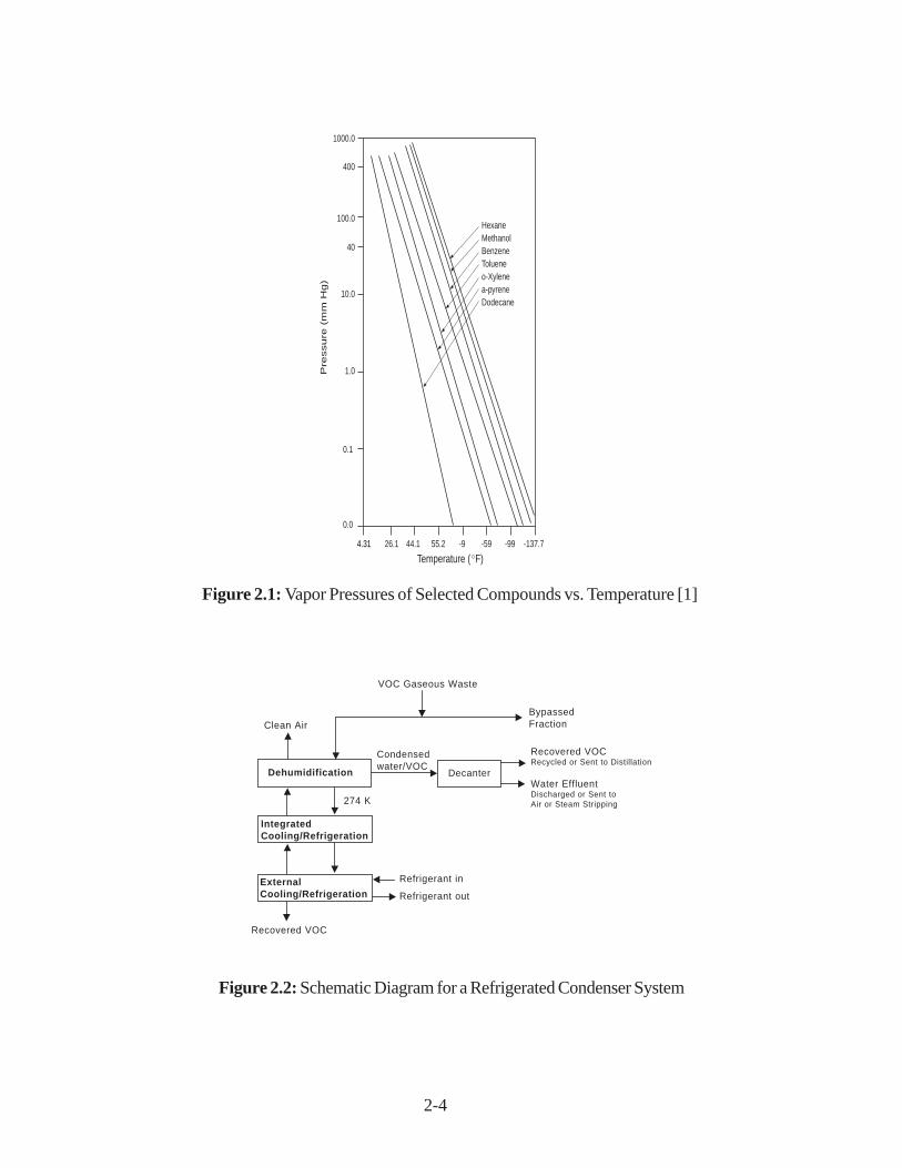
The removal efficiency of a condenser is dependent on the emission stream characteristicsincluding the nature of the VOC in question (vapor pressure/temperature relationship), VOCconcentration, and the type of coolant used. Any component of any vapor mixture can be condensedif brought to a low enough temperature and allowed to conic to equilibrium. Figure 2.1 shows thevapor pressure dependence on temperature for selected compounds.[1] A condenser cannot lowerthe inlet concentration to levels, below the saturation concentration at the coolant temperature.Removal efficiencies above 90 percent can be achieved with coolants such as chilled water, brinesolutions, ammonia, or chlorofluorocarbons, depending on the VOC composition andconcentration level of the emission stream.

2.2 Process Description

Figure 2.2 depicts a typical configuration for a refrigerated surface condenser system as anemission control device. The basic equipment required for a refrigerated condenser system includesa VOC condenser, a, refrigeration unit(s). and auxiliary, equipment (e.g., precooler, recovery/storage tank, pump/blower, and piping).

2-4

Figure 2.1: Vapor Pressures of Selected Compounds vs. Temperature [1]

Clean Air

274 K

Decanter

Recovered VOCRecycled or Sent to Distillation

Water EffluentDischarged or Sent to Air or Steam Stripping

ExternalCooling/Refrigeration

Refrigerant in

Refrigerant out

Recovered VOC

Bypassed Fraction

Condensed water/VOC

Dehumidification

Integrated Cooling/Refrigeration

VOC Gaseous Waste

Figure 2.2: Schematic Diagram for a Refrigerated Condenser System

Temperature ( F)

HexaneMethanolBenzeneTolueneo-Xylenea-pyreneDodecane

Pre

ssu

re (

mm

Hg

)

4.31

0.0

0.1

1.0

10.0

40

100.0

400

1000.0

26.1 44.1 55.2 -9 -59 -99 -137.7

2-5

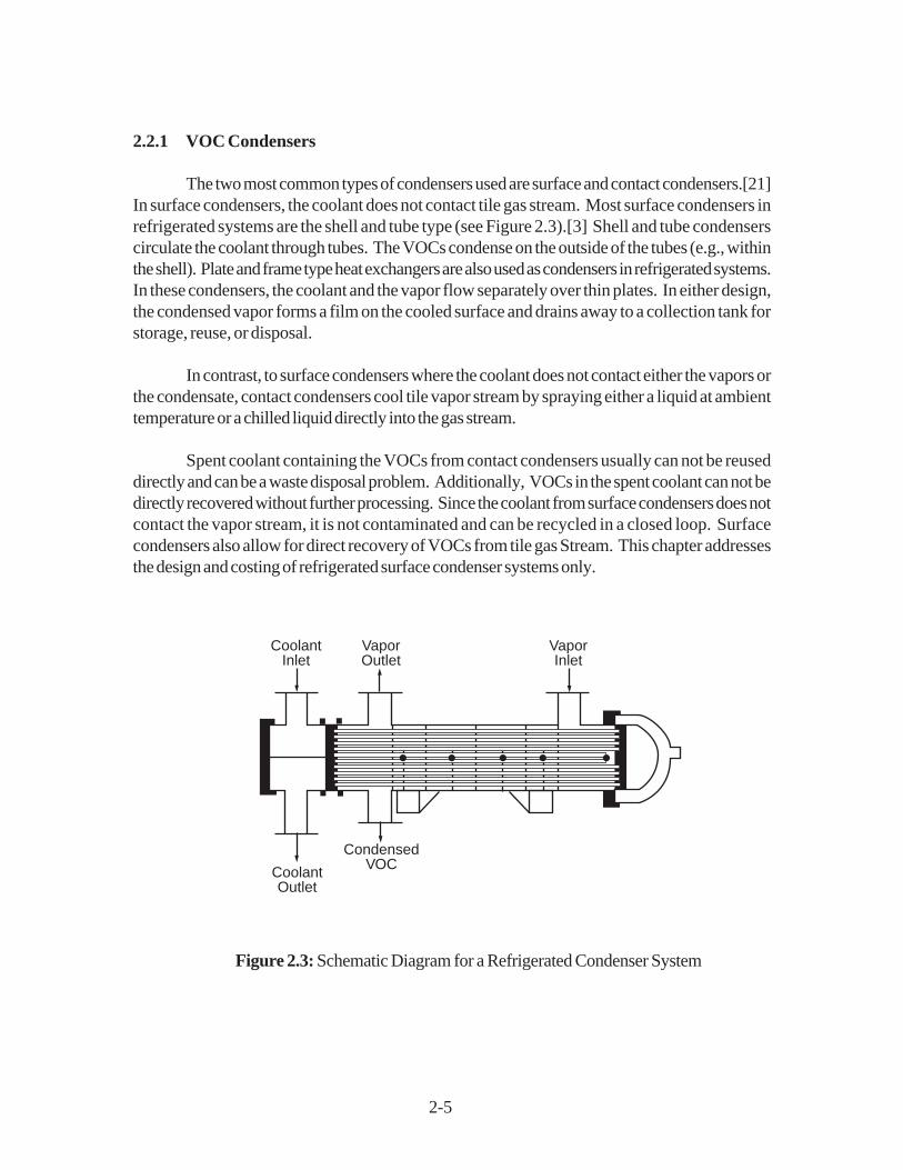
2.2.1 VOC Condensers

The two most common types of condensers used are surface and contact condensers.[21]In surface condensers, the coolant does not contact tile gas stream. Most surface condensers inrefrigerated systems are the shell and tube type (see Figure 2.3).[3] Shell and tube condenserscirculate the coolant through tubes. The VOCs condense on the outside of the tubes (e.g., withinthe shell). Plate and frame type heat exchangers are also used as condensers in refrigerated systems.In these condensers, the coolant and the vapor flow separately over thin plates. In either design,the condensed vapor forms a film on the cooled surface and drains away to a collection tank forstorage, reuse, or disposal.

In contrast, to surface condensers where the coolant does not contact either the vapors orthe condensate, contact condensers cool tile vapor stream by spraying either a liquid at ambienttemperature or a chilled liquid directly into the gas stream.

Spent coolant containing the VOCs from contact condensers usually can not be reuseddirectly and can be a waste disposal problem. Additionally, VOCs in the spent coolant can not bedirectly recovered without further processing. Since the coolant from surface condensers does notcontact the vapor stream, it is not contaminated and can be recycled in a closed loop. Surfacecondensers also allow for direct recovery of VOCs from tile gas Stream. This chapter addressesthe design and costing of refrigerated surface condenser systems only.

VaporInlet

VaporOutlet

CoolantInlet

CoolantOutlet

CondensedVOC

Figure 2.3: Schematic Diagram for a Refrigerated Condenser System

2-6

2.2.2 Refrigeration Unit

The commonly used mechanical vapor compression cycle to produce refrigeration consistsof four stages: evaporation, compression, condensation, and expansion (see Figure 2.4).[4] Tilecycle which is used for single-stage vapor compression involves two pressures, high and low, toenable a continuous process to produce a cooling effect. Heat absorbed from tile gas streamevaporates the liquid coolant (refrigerant). Next, the, refrigerant (now in vapor phase) iscompressed to a higher temperature and pressure by tile system compressor. Then, the superheatedrefrigerant vapor is condensed, rejecting its sensible and latent heat in the condenser. Subsequently,the liquid refrigerant flows from the condenser through the expansion valve, where pressure andtemperature are reduced to those in the evaporator, thus completing the cycle.

The capacity of a refrigeration unit is the rate at which heat is removed, expressed in tonsof refrigeration. One ton of refrigeration is the refrigeration produced by melting one ton of ice at32°F in 24 hours. It is the rate of removing heat equivalent to 12,000 Btu/h or 200 Btu/min. Formore details on refrigeration principles, see References [5] and [6].

Applications requiring low temperatures (below about -30°F), multistage refrigerationsystems are frequently employed.[4] Multistage systems are designed and marketed in two differenttypes-compound and cascade. In compound systems, only one refrigerant is used. In a cascadesystem, two or more separate refrigeration systems are interconnected in such a manner that oneprovides a means of heat rejection for the other. Cascade systems are desirable for applicationsrequiring temperatures between -50 and -150°F and allow the use of different refrigerants in eachcycle,[4] Theoretically, any number of cascaded stages are possible, each stage requiring anadditional condenser and an additional stage of compression.

ExpansionValve

Evaporator

Low Pressure Side Compressor

High Pressure Side

Condenser

Figure 2.4: Basic Refrigeration Cycle [4]

2-7

In refrigerated condenser systems, two kinds of refrigerants are used, primary andsecondary. Primary refrigerants are those that undergo a phase change from liquid to gas afterabsorbing heat. Examples are ammonia (R-717), and chlorofluorocarbons such aschlorodifluoromethane (R-22) or dichlorodifluorormethane (R-12). Recent concerns about thelatter causing depletion of the ozone layer is prompting development of substitute refrigerants.Secondary refrigerants such as brine solutions act only as heat carriers and remain in liquid phase.

Conventional systems use a closed primary refrigerant loop that cools the secondary loopthrough the heat transfer medium in the evaporator. The secondary heat transfer fluid is then pumpedto a VOC vapor condenser where it is used to cool the, air/VOC vapor stream. In someapplications. however, the primary refrigeration fluid is directly used to cool the vapor stream.

2.2.3 Auxiliary Equipment

As shown in Figure 2.2, some applications may require auxiliary equipment such asprecoolers, recovery/storage tanks, pumps/blowers, and piping.

If water vapor is present in the treated gas stream or if the VOC has a high freezing point(e.g., benzene), ice or frozen hydrocarbons may form on the condenser tubes or plates. This willreduce the heat transfer efficiency of the condenser and thereby reduce the removal efficiency.Formation of ice will also increase the pressure drop across the condenser. In such cases, aprecooler may be needed to condense the moisture prior to the VOC condenser. This precoolerwould bring the temperature of the stream down to approximately 35 to 40°F, effectively removingthe moisture from the gas. Alternatively, an intermittent heating cycle can be used to melt away icebuild-up. This may be accomplished by circulating ambient temperature brine through the condenseror by the use of radiant heating coils. If a system is not operated continuously, the ice can also beremoved by circulating ambient air.

A VOC recovery tank for temporary storage of condensed VOC prior to reuse,reprocessing, or transfer to a larger storage tank may be necessary in some cases. Pumps andblowers are typically used to transfer liquid (e.g., coolant or recovered VOC) and gas streams,respectively, within the system.

2.3 Design Procedures

In this section are presented two procedures for designing (sizing) refrigerated surfacecondenser systems to remove VOC from air/VOC mixtures. With the first procedure presented,one calculates the condenser exit temperature needed to obtain a given VOC recovery efficiency.In the second procedure, which is the inverse of the first, the exit temperature is given and the recoverefficiency corresponding to it is calculated.

2-8

The first procedure depends on knowledge of the following parameters:

1. Volumetric flow rate of the VOC-containing gas stream;

2. Inlet temperature of the gas stream;

3. Concentration and composition of the VOC in the gas stream;

4. Required removal efficiency of the VOC;

5. Moisture content of the emission stream; and

6. Properties of the VOC (assuming the VOC is a pure compound):

• Heat of condensation,

• Heat capacity, and

• Vapor pressure.

The design of a refrigerated condenser system requires determination of the VOCcondenser size and the capacity of the refrigeration unit. For a given VOC removal efficiency, thecondensation temperature and the heat load need to be calculated to determine these parameters.The data necessary to perform the sizing procedures below as well as the variable names and theirrespective units are listed in Table 8.1.

Table 8.1: Required Input Data

Data Variable Name Units

Inlet Stream Flow Rate Qin

SCFM (770F:1 atm)Inlet Stream Temperature T

in0F

VOC Inlet Volume Fraction Yvoc

,in volume fractionRequired VOC Removal Efficiency n -Antoine Equation Constantsa A,B,C Btu/lb-moleHeat of Condensation of the VOCa deltaH Btu/lb-mole-0FHeat Capacity of the VOCa C

p,voc Btu/lb-0F

Specific Heat of the Coolant Cp,cool

Btu/lb-mole-0FHeat Capacity of Air C

p,air

aSee Appendix A for these properties of selected organic compounds.

2-9

The steps outlined below for estimating condensation temperature and the heat load applyto a two-component mixture (VOC/air) in which one of the two components is considered to benoncondensible (air). The VOC component is assumed to consist of a single compound. Also, theemission stream is assumed to be free of moisture. The calculations are based on the assumptionsof ideal gas and ideal solution to simplify the sizing procedures. For a more rigorous analysis, SeeReference [5].

2.3.1 Estimating Condensation Temperature

The temperature necessary to condense the required amount of VOC must, be estimatedto determine the heat load. The first step is to determine the VOC concentration at the outlet of thecondenser for a given removal efficiency. This is calculated by first determining the partial pressureof the VOC at the outlet, P

voc. Assuming that the ideal gas law applies, P

voc is given by:

( )P ou tle tM o les V O C in ou tle t s tream

M oles in le t s tream - M o les V O C rem ovedV O C = 760 (2.1)

where

PVOC

= Partial pressure of the VOC in the exit stream (mm Hg).

and the condenser is assumed to operate at a constant pressure of one atmosphere (760mm Hg).

However:

Moles VOC in outlet stream = (Moles VOC in inlet stream)(1-�) (2.2)Moles VOC in inlet stream = (Moles in inlet stream) y

voc,in(2.3)

Moles VOC removed = (Moles VOC in inlet stream) (2.4)where

� = removal efficiency of the condenser system (fractional)= Moles VOC removed/Moles VOC in inlet

yvoc,in

= Volume fraction of VOC in inlet stream

After substituting these variables in Equation 2.1, we obtain:

( )[ ]P = -

- V O C

V O C , in

V O C , in

7601

1

y

y

( )η

η

(2.5)

2-10

At the condenser outlet, the VOC in the gas stream is assumed to be at equilibrium with theV0C condensate. At equilibrium, the partial pressure of the VOC in the gas stream is equal to itsvapor pressure at that temperature assuming the condensate is pure VOC (e.g., vapor pressureP

voc). Therefore, by determining the temperature at which this condition occurs, the condensation

temperature can be specified. This calculation is based on the Antoine equation that defines therelationship between vapor pressure and temperature for a particular compound:

P = A - B

T + CV O Ccon

log (2.6)

where Tcon

is the condensation temperature (°C). Note that Tcon

is in degrees Centigrade in thisequation. In Equation 2.6, A, B, and C are VOC-specific constants pertaining to temperatureexpressed in °C and pressure in mm Hg (see Appendix 8A). Solving for T

con and converting to

degrees Fahrenheit:

( )T = B

A - P - C + con

V O Clog.

10

1 8 32

(2.7)

The calculation methods for a gas stream containing multiple VOCs are complex,particularly when there are significant departures from the ideal behavior of gases and liquids.However, the temperature necessary for condensation of a mixture of VOCs can be estimated bythe weighted average of the temperatures necessary to condense each VOC in the gas stream at aconcentration equal to the total VOC concentration.[1]

2.3.2 VOC Condenser Heat Load

Condenser heat load is the amount of heat that must be removed from the inlet stream toattain the specified removal efficiency. It is determined from an energy balance, taking into accountthe enthalpy change due to the temperature change of the VOC, the enthalpy change due to thecondensation of the VOC, and the enthalpy change due to the temperature change of the air.Enthalpy change due to the presence of moisture in the inlet gas stream is neglected in the followinganalysis.

For the purpose of this estimation, it is assumed that, the total heat load on the system is equalto the VOC Condenser heat load. Realistically, when calculating refrigeration capacity requirements

2-11

for low temperature cooling units, careful consideration should be given to the, process line, lossesand heat input of the process pumps. Refrigeration unit capacities are typically rated in terms of netoutput and do not reflect any losses through process pumps or process lines.

First, the number of lb-moles of VOC per hour in the inlet stream must be calculated by thefollowing expression:

( )MQ

fty

m in

hrV O C , in in

V O C , iu= 392

603 (2.8)

where Mvoc,in is the molar flow rate of VOC in the inlet stream and Q is the volume flow rate instandard ft3/min(scfm). The factor 392 is the volume (ft3) occupied by one lb-mole of inlet gas streamat standard conditions (77°F and 1 atm). The number of lb-moles of VOC per hour in the outletgas stream is calculated as follows:

M Mvoc voc, , ( ) ou t in = - 1 η (2.9)

where Mvoc,out is the molar flow rate of VOC in the exit stream. Finally, the number of lb-moles ofVOC per hour that are condensed is calculated as follows:

M = M - Mvo c, c on vo c , in vo c , o u t (2.10)

where Mvoc,con

is the flow rate of the VOC that is condensed.

The condenser heat load is then calculated by the following equation:

H = H + H + Hload con uncon non con∆ ∆ ∆ (2.11)

whereH

load= condenser heat load (Btu/hr)

Hcon

= enthalpy change associated with the condensed VOC (Btu/hr)H

uncon= enthalpy change associated with the uncondensed VOC (Btu/lir)

Hnoncon

= enthalpy change associated with the noncondensible air (Btu/hr).

The change in enthalpy of the condensed VOC is calculated as follows:

( )[ ]∆ ∆H = M H + C T - Tco n V O C , co n V O C p , V O C in co n (2.12)

2-12

where Hvoc

is the molar heat of condensation and Cp,voc is the molar heat capacity of the VOC. Eachparameter varies as function of temperature. In Equation 8.12, H

voc and Cp,voc are evaluated at the

mean temperature:

TT in T

m eancon=

+2

(2.12a)

The heat of condensation at a specific temperature, T2, (°R), can be calculated from the heat

of condensation at a reference temperature, T1 (°R), using the Watson Equation:[7]

( ) ( )∆ ∆H T = H T

- T

T

- T

T

V O C V O Cc

c

a t a t2 1

2

1

0 38

1

1

.

(2.13)

where Tc (°R) is the VOC critical temperature.

The heat capacity can also be calculated for a specific temperature, T2, if heat capacity

constants (a, b, c, and d) are known for the particular compound. The heat capacity equation is:

C = a + b T + cT + d Tp , vo c 2 22

23

(2.14)

However, to simplify the heat load analysis, Cp,voc can be assumed to remain constant over thetemperature range of operation (i.e., Tin - Tcon) without much loss of accuracy in the heat loadcalculations, as the sensible heat change in Equation 8.12 is relatively small compared to the enthalpychange due to condensation.

Heat of condensation and heat capacity data are provided in Appendix A. The heat ofcondensation for each compound is reported at its boiling point, while its heat capacity is given at77°F. To estimate the heat of condensation at another temperature, use Equation 2.13. However,the Appendix A heat capacity data may be used to approximate Cp,voc at other temperatures, sincesensible heat changes are usually small, compared to condensation enthalpy changes.

The enthalpy change associated with the uncondensed VOC is calculated by the followingexpression:

2-13

( )H = M C T - Tuncon V O C , ou t p , V O C in con (2.15)

Finally, the enthalpy change of the noncondensible air is calculated as follows:

( )∆H = Q

- M C T - Tnon conin

V O C , in p , air in con392603ft

m in

hr

(2.16)

where Cp,air

is the specific heat of air. In both Equations 2.15 and 2.16, the Cp’s are evaluated at

the mean temperature, as given by Equation 2.12a.

2.3.3 Condenser Size

Condensers are sized based on the heat load, the logarithmic mean temperature differencebetween the emission and coolant streams, and the overall heat transfer coefficient. The overall heattransfer coefficient, U, can be estimated from individual heat transfer coefficients of the gas streamand the coolant. The overall heat transfer coefficients for tubular heat exchangers where organicsolvent vapors in noncondensible gas are condensed on the shell side and water/brine is circulatedon the tube side typically range from 20 to 60 Btu/hr-ft2-°F according to Perry’s ChemicalEngineers’ Handbook[4]. To simplify the calculations, a single “U” value may be used to size thesecondensers. This approximation is acceptable for purposes of making study cost estimates.

Accordingly, an estimate of 20 Btu/hr-ft2-°F can be used to obtain a conservative estimateof condenser size. The following equation is used to determine the required heat transfer area:

A = H

U Tconload

lm∆ (2.17)

whereA

con = condenser surface area (ft2)

U = overall heat transfer coefficient (Btu/hr-ft2-°F)T

lm= logarithmic mean temperature difference (°F).

The logarithmic mean temperature difference is calculated by the following equation, which is basedon the use of a countercurrent flow condenser:

2-14

( ) ( )∆T =

T - T - T - T

T - T

T - T

lmin coo l, ou t con coo l, in

in coo l, ou t

con coo l, in

ln

(2.18)

whereT

cool,in = coolant inlet temperature (°F)

Tcool,out

= coolant outlet temperature (°F).

The temperature difference (“approach”) at the condenser exit can be assumed to be 15°F.In other words, the coolant inlet temperature, T

cool,in, will be 15°F less than the calculated

condensation temperature, Tcon

. Also, the temperature rise of the coolant is specified as 25°F.(These two temperatures- the condenser approach and the coolant temperature rise-reflect gooddesign practice that, if used, will result in an acceptable condenser size.) Therefore, the followingequations can be applied to determine the coolant inlet and outlet temperature:

T = Tcool, in con - F15 � (2.19)

T = Tcool, o u t coo l, in + F25 � (2.20)

2.3.4 Coolant Flow Rate

The heat removed from the emission stream is transferred to the coolant. By a simple energybalance, the flow rate of the coolant can be calculated as follows:

( )W = H

C T - Tco o l

loa d

p , c oo l co o l, o ut co o l, in(2.21)

where Wcool is the coolant flow rate (lb/hr), and Cp,cool is the coolant specific heat (Btu/lb-°F). Cp,cool

will vary according to the type of coolant used. For a 50-50 (volume %) mixture of ethylene glycoland water, Cp,cool

is approximately 0.65 Btu/lb-°F. The specific heat of brine (salt water), anothercommonly used coolant, is approximately 1.0 Btu/lb-°F.

2-15

2.3.5 Refrigeration Capacity

The refrigeration unit is assumed to supply the coolant at the required temperature to thecondenser. The required refrigeration capacity is expressed in terms of refrigeration tons as follows:

R = H load

1 2 0 00, (2.22)

Again, as explained in section 2.3.2, Hload

does not include any heat losses.

2.3.6 Recovered VOC

The mass of VOC recovered in the condenser can be calculated using the followingexpression:

W = M M Wvoc, co n voc , co n voc× (2.23)

whereW

voc,con = mass of VOC recovered (or condensed) (lb/hr)

MWvoc

= molecular weight of the VOC (lb/lb-mole).

2.3.7 Auxiliary Equipment

The auxiliary equipment for a refrigerated surface condenser system may include:

• precooler,• recovered VOC storage tank,• pumps/blowers, and• piping/ductwork.

If water vapor is present in the treated gas stream, a precooler may be needed to removemoisture to prevent ice from forming in the VOC condenser. Sizing of a precooler is influenced bythe moisture concentration and the temperature of the emission stream. As discussed in Section2.2.3, a precooler may not be necessary for intermittently operated refrigerated surface condensersystems where the ice will have time to melt between successive operating periods.

If a precooler is required, a typical operating temperature is 35 to 40°F. At this temperature,almost all of the water vapor present will be condensed without danger of freezing. Thesecondensation temperatures roughly correspond to a removal efficiency range of 70 to 80 percent

2-16

if the inlet stream is saturated with water vapor at 77°F. The design procedure outlined in theprevious sections for a VOC condenser can be used to size a precooler, based on the psychometricchart for the air-water vapor system (see Reference [4]).

Storage/recovery tanks are used to store the condensed VOC when direct recycling is nota suitable option. The size of these tanks is determined from the amount of VOC condensate to becollected and the amount of time necessary before unloading. Sizing of pumps and blowers is basedon the liquid and gas flow rates, respectively, as well as the system pressure drop between the inletand outlet. Sizing of the piping and ductwork (length and diameter) primarily depends upon thestream flow rate, duct/pipe velocity, available space, and system layout.

2.3.8 Alternate Design Procedure

In some applications, it may be desirable to size and cost a refrigerated condenser systemthat will use a specific coolant and provide a particular condensation temperature. The designprocedure to be implemented in such a case would essentially be the same as the one presented inthis section except that instead of calculating the condenser exit temperature needed to obtain aspecified VOC recovery efficiency, the exit temperature is given and the corresponding recoveryefficiency is calculated.

The initial calculation would be to estimate the partial (=vapor) pressure of the VOC at thegiven condenser exit temperature, T

con, using Equation 2.6. Next, calculate η using Equation 2.24,

by rearranging Equation 2.5:

( )( )η =

- P

- P

V O C , in V O C

V O C , in V O C

760

760

y

y(2.24)

Finally, substitute the calculated Pvoc

into this equation to obtain η. In the remainder of thecalculations to estimate condenser heat load, refrigeration capacity, coolant flow rate, etc., followthe procedure presented in Sections 2.3.2 through 2.3.7.

2.4 Estimating Total Capital Investment

This section presents the procedures and data necessary for estimating capital costs forrefrigerated surface condenser systems in solvent vapor recovery and gasoline vapor recoveryapplications. Costs for packaged and nonpackaged solvent vapor recovery systems are presentedin Sections 2.4.1 and 2.4.2, respectively. Costs for packaged gasoline vapor recovery systems are

2-17

described in Section 2.4.3. Costs are calculated based on the design/sizing procedures discussedin Section 2.3.

Total capital investment, TCI, includes equipment cost, EC, for the entire refrigeratedcondenser unit, auxiliary equipment costs, taxes, freight charges, instrumentation, and direct, andindirect installation costs. All costs in this chapter are presented 3rd quarter 1990 dollars.1

For these control systems, the total capital investment is a battery limit cost estimate anddoes not include the provisions for bringing utilities, services, or roads to the site; the, backupfacilities; the land; the working capital, the research and development required; or the process pipingand instrumentation interconnections that may be required in the process generating tile waste gas.These costs are based on new plant installations; no retrofit cost considerations are included. Theretrofit cost factors are so site specific that no attempt has been made to provide them.

The expected accuracy of the cost estimates presented in this chapter is ±30 percent (e.g..,“study” estimates). It must be kept in mind that even for a given application, design andmanufacturing procedures vary from vendor to vendor, so costs may vary.

In the next two sections, equipment costs are presented for packaged and nonpackaged(custom) solvent vapor recovery systems. respectively. With the packaged systems the equipmentcost is factored from the refrigeration the custom systems, the equipment cost is determined as thesum of the costs of the individual system components. Finally. equipment costs for packagedgasoline, vapor recovery systems are given in Section 2.4.3.

2.4.1 Equipment Costs for Packaged Solvent Vapor Recovery Systems

Vendors were asked to provide refrigerated unit cost estimates for a wide range ofapplications. The equations shown below for refrigeration unit equipment costs, EC

r, are

multivariable regressions of data provided by two vendors and are only valid for the ranges listedin Table 2.2.[8,9] In this table, the capacity range of refrigeration units for which cost data wereavailable are shown as a function of temperature.

Single Stage Refrigeration Units (less than 10 tons)

( )E C .r con = - T + R9 83 0 014 0 340. . ln (2.25)

2-18

Table 1.2: Applicability Ranges for the Refrigeration Unit Cost Equations(Equations 8.25 to 8.27)

Temperature Minimum Size Available Maximum Size AvailableTcon(

oF)a R(tons) R(tons) R(tons)

Single Stage Multistage Single Stage Multistage40 0.85 NAb 174 NA30 0.63 NA 170 NA20 0.71 NA 880 NA10 0.44 NA 200 NA

0 to -5 0.32 NA 133 NA-10 0.21 3.50 6.6 81

-20 to -25 0.13 2.92 200 68-30 NA 2.42 NA 85-40 NA 1.92 NA 68

-45 to -50 NA 1.58 100c 55-55 to -60 NA 1.25 100c 100

-70 NA 1.33 NA 42-75 to -80 NA 1.08 NA 150

-90 NA 0.83 NA 28-100 NA 0.67 NA 22

aFor condensation temperatures that lie between the levels shown, round off to the nearest level (e.g., if Tcon

= 16°F, use 20°F) to determineminimum and maximum available size.bNA = System not available based on vendor data collected in this study.cOnly one data point available.

Single Stage Refrigeration Units (greater than or equal to 10 tons)

( )E C . .r con = - T + R9 26 0 007 0 627. ln (2.26)

Multistage Refrigeration Units

EC = exp (9.73 - 0.012T

con + 0.584 ln R) (2.27)

Equations 2.25 and 2.26 provide costs for refrigeration units based on single stage designs,while Equation 2.27 gives costs for multistage units. Equation 2.27 covers both types of multistageunits, “cascade” and “compound”. Data provided by a vendor show that the costs of cascade and

2-19

compound units compare well, generally differing by less than 30%.[8] Thus, only one cost equationis provided. Equation 2.25 applies to single stage refrigeration units smaller than 10 tons andEquation 2.26 applies to single stage refrigeration units as large or larger than 10 tons. Single stageunits typically achieve temperatures between 40 and -20°F, although there are units that are capableof achieving -60°F in a single stage.[8, 10] Multistage units are capable of lower temperatureoperation between -10 and -100°F.

0

20,000

40,000

60,000

80,000

100,000

120,000

140,000

160,000

180,000

200,000

0 20 40 60 80 100Capacity

(tons)

Equ

ipm

ent C

ost,

3rd

Qua

rter

199

0 D

olla

rs -20oF 0oF 20oF40oF

Figure 2.5: Refrigeration Unit Equipment Cost (Single Stage) [8.9]

Single stage refrigeration unit costs are depicted graphically for selected temperatures inFigure 2.5. Figure 2.6 shows the equipment cost curves for multistage refrigeration units.

(NOTE: In Figure 2.5, the discontinuities in the curves at the 10 ton capacity are a result of the tworegression equations used. Equation 2.25 is used for capacities of less than 10 tons; Equation 2.26is used for capacities greater than or equal to 10 tons.)

These costs are for outdoor models that are skid-mounted on steel beams and consist ofthe following components: walk-in weatherproof enclosure, air-cooled low temperaturerefrigeration machinery with dual pump design, storage reservoir, control panel and instrumentation,vapor condenser, and necessary piping. AR refrigeration units have two pumps: a system pump anda bypass pump to short-circuit the vapor condenser during no-load conditions. Costs for heattransfer fluids (brine) are not included.

2-20

The equipment cost of packaged solvent vapor recovery systems (ECp) is estimated to be

25 percent greater than the cost of the refrigeration unit alone [9]. The additional cost includes VOCcondenser, recovery tank, the necessary connections, piping, and additional instrumentation. Thus:

E C . E Cp r = 1 2 5 (2.28)

Purchased equipment cost, PEC, includes the packaged equipment cost, ECp, and factors

for sales taxes (0.03) and freight (0.05). Instrumentation and controls are included with thepackaged units. Thus,

( )P E C E C + . + . . E Cp p p = = 1 0 03 0 05 1 08 (2.29)

2.4.2 Equipment Costs for Nonpackaged (Custom) Solvent Vapor Recovery Systems

To develop cost estimates for nonpackaged or custom refrigerated systems, informationwas solicited from vendors on costs of refrigeration units, VOC condensers, and VOC storage/recovery tanks [9, 11, 12]. Quotes from the vendors were used to develop the estimated costs foreach type of equipment. Only one set of vendor data was available for each type of equipment.

Equations 2.25, 2.26, and 2.27 shown above are applicable for estimating the costs for the

0

100,000

200,000

300,000

400,000

500,000

600,000

700,000

0 20 40 60 80 100

Capacity (tons)

Equ

ipm

ent C

ost,

3rd

Qua

rter

199

0 D

olla

rs

-20o F

-30o F-40o F

-60o F

-80o F

-100o F

Figure 2.6: Refrigeration Unit Equipment Cost (Multistage) [9]

2-21

refrigeration units. Equation 8.30 shows the equation developed for the VOC condenser costestimates[11]:

E C con con = A + 3 4 3 7 5 5, (2.30)

This equation is valid for the range of 38 to 800 ft2 and represents costs for shell arid tube type heatexchangers with 304 Stainless Steel tubes.

The following equation represents the storage/recovery tank cost data obtained from onevendor[12]:

E C tank tank = V + 2 7 2 1 9 60. , (2.31)

These costs are applicable for the range of 50 to 5,000 gallons and pertain to 316 stainlesssteel vertical tanks.

Costing procedures for a precooler (ECpre

) that includes a separate condenser/refrigerationunit and a recovery tank are similar to that for a custom refrigerated condenser system. Hence,Equations 2.25 through 2.31 would be applicable, with the exception of Equation 2.27, whichrepresents multistage systems. Multistage systems operate at much lower temperatures than thatrequired by a precooler.

Costs for auxiliary equipment such as ductwork, piping, fans, or pumps are designated asEC

auz, These items should be costed separately using methods described elsewhere in this Manual.

The total equipment cost for custom systems, ECc is then expressed as:

E C = E C + E C + E C + E C + E Cc r co n ta n k p re a u x (2.32)

The purchased equipment cost including ECc and factors for sales taxes (0.03), freight

(0.05), and instrumentation and controls (0.10) is given below:

( )P E C E C E Cc c c = + + + = 1 0 03 0 05 0 10 1 18. . . . (2.33)

2.4.3 Equipment Costs for Gasoline Vapor Recovery Systems

Separate quotes were obtained for packaged gasoline vapor recovery systems becausethese systems are specially designed for controlling gasoline vapor emissions from such sources asstorage tanks, gasoline bulk terminals, and marine vessel loading and unloading operations. Systemsthat control marine vessel gasoline loading and unloading operations also must meet U.S. Coast

2-22

Guard safety requirements.

Quotes obtained from one vendor were used to develop equipment cost estimates for thesepackaged systems (see Figure 2.7). The cost equation shown below is a least squaresregression of these cost data and is valid for tile range 20 to 140 tons.[91]

E C Rp = + 4 9 1 0 2 1 2 0 0 0, , (2.34)

The vendor data in process flow capacity (gal/min) vs cost ($) were transformed into Equation 2.34after applying the design procedures in Section 2.3. Details of the data transformation are given inAppendix B.

The cost estimates apply to skid-mounted refrigerated VOC condenser systems forhydrocarbon vapor recovery primarily at gasoline loading/storage facilities. The systems areintermittently operated at -80 to -120°F allowing 30 to 60 minutes per day for defrosting bycirculation of warm brine. Multistage systems are employed to achieve these lower temperatures.Tile achievable VOC removal efficiencies for these systems are in the range of 90 to 95 percent.

The packaged systems include the refrigeration unit with the necessary pumps,compressors, condensers/evaporators, coolant reservoirs, the VOC condenser unit and VOCrecovery tank, precooler, instrumentation and controls, and piping. Costs for heat transfer fluids(brines) are not included. The purchased equipment cost for these systems includes sales tax andfreight and is calculated using Equation 2.29.

Figure 2.7: Gasoline Vapor Recovery System Equipment Cost [9]

0

200,000

400,000

600,000

800,000

0 20 40 60 80 100 120

Capacity (tons)

Equ

ipm

ent C

ost,

3rd

Qua

rter

199

0 D

olla

rs

0 2,000 4,000 6,000 8,000 10,000Capacity (gal/min)

2-23

Table 2.3: Capital Cost Factors for Nonpackaged (Custom)Refrigerated Condenser Systems

Cost Item Factor

Purchased Equipment CostsRefrigerated condenser system, EC As estimated, AInstrumentation 0.10 ASales Taxes 0.03 AFreight 0.05 APurchased equipment costs, PEC B=1.18 Aa

Direct Installation Costs 0.08 BFoundations & Supports 0.14 BHandling & Erection 0.08 BElectrical 0.08 BPiping 0.02 BInsulation 0.10 BPainting 0.01 BDirect Installation Costs 0.43 B

Site Preparation As Required, SPBuildings As Required, Bldg.

Total Direct Costs, DC 1.43 B + SP + Bldg.

Indirect Costs (Installation)Engineering 0.10 BConstruction and Field Expenses 0.05 BContractor Fees 0.10 BStart-Up 0.02 BPerformance Test 0.01 BContingencies 0.03 BTotal Indirect Costs, IC 0.31 B

Total Capital Investment = DC + IC 1.74 b + SP + Bldg.b

a Purchased equipment cost factor for packaged systems is 1.08 with instrumentation included.b For packaged systems, total capital investment = 1.15PEC

p.

2-24

Table 2.4: Suggested Annual Cost Factors for Refrigerated Condenser Systems

Cost Item Factor

Direct Annual Cost, DCOperating Labor 1/2 hour per shiftOperator 15% of operatorSupervisor

Operating Materials

MaintenanceLabor 1/2 hour per shiftMaterial 100% of maintenance labor

Electricityat 40oF 1.3 kW/tonat 20oF 2.2 kW/tonat -20oF 4.7 kW/tonat -50oF 5.0 kW/tonat -100oF 11.7 kW/ton

Indirect Annual Costs, ICOverhead 60% of total labor and

maintenance material costsAdministrative Charges 2% of Total Capital InvestmentProperty Tax 1% of Total Capital InvestmentInsurance 1% of Total Capital InvestmentCapital Recoverya 0.1098 x Total Capital Investment

Recovery Credits, RCRecoverd VOC Quality recovered x operating hours

Total Annual Cost DC + IC - RC

a Assuming a 15 year life at 7% [13]. See Chapter 2.

2-25

T C I P E C = p1 1 5. (2.35)

For nonpackaged (custom) systems, the total installation factor is 1.74:

T C I P E C = c1 7 4. (2.36)

An itemization of tile total installation factor for nonpackaged systems is shown in Table 2.3.Depending on the site conditions., the installation costs for a given system could deviatesignificantly, from costs generated by there average factors. Guidelines are available foradjusting these average installation factors.[14]

2.5 Estimating Total Annual Cost

The total annual cost (TAC) is the sum of the direct and indirect annual costs. Thebases used in calculating annual cost factors are given in Table 2.4.

2.5.1 Direct Annual Costs

Direct annual costs, DC, include-labor (operating and supervisory), maintenance (laborand materials), and electricity. Operating labor is estimated at 1/2-hour per 8-hour shift. Thesupervisory labor cost is estimated at 15% of the operating labor cost. Maintenance labor is

2.4.4 Installation Costs

The total capital investment, TCl, for packaged systems is obtained by multiplying thepurchased equipment cost, PEC

p by the total installation factor:[13]

Table 2.5: Electricity Requirements

Electricity (E, kW/ton) Temperature (oF)1.3 402.2 204.7 -205.0 -5011.7 -100

2-26

estimated at 1/2-hour per 8-hour shift.

Maintenance materials costs are assumed to equal maintenance labor costs.Utility costs for refrigerated condenser systems include electricity requirements for the

refrigeration unit and any pumps/blowers. The power required by the pumps/blowers isnegligible when compared with the refrigeration unit power requirements. Electricityrequirements for refrigerated condenser systems are summarized in Table 2.5:These estimates were developed from product literature obtained from one vendor.[9] Theelectricity cost, C

e, can then be calculated from the following expression:

CR

E pecom pressor

e = s ηθ (2.37)

where θ

s= system operating hours (hr/yr)

pe

= electricity cost η

compressor = mechanical efficiency of the compressor

2.5.2 Indirect Annual Costs

Indirect annual costs, IC, are calculated as the sum of capital recovery costs plusgeneral and administrative (G&A), overhead, property tax, and insurance costs. Overhead isassumed to be equal to 60 percent of the sum of operating, supervisory, and maintenance labor,and maintenance materials. Overhead cost is discussed in Section 1 of this Manual.

The system capital recovery cost, CRC, is based on an estimated 15-year equipmentlife.[13] (See Section 1 of the Manual for a discussion of the capital recovery cost.) For a 15-year life and an interest rate of 7 percent, the capital recovery factor is 0.1098. The systemcapital recovery cost is then estimated by:

CR

E pecom pressor

e = s ηθ (2.37)

2-27

G&A costs, property tax, and insurance are factored from total capital investment.typically at 2 percent, 1 percent, and 1 percent, respectively.

Table 2.6: Example Problem Data

Vent Stream Parameters Value

Inlet Stream Flow Rate 100 scfma

Inlet Stream Temperature 86oFVOC to be Condensed AcetoneVOC Inlet Volume Fraction 0.0375Required VOC Removal Efficiency .90

Antoine Equation Constants for Acetone:A 7.117B 1210.595C 229.664

Heat of Condensation of Acetoneb 12,510 Btu/lb-moleHeat Capacity of Acetonec 17.90 Btu/lb-mole-oFSpecific Heat of Coolantc (ethylene glycol) 0.65 Btu/lb-oFHeat Capacity of Airc 6.95 Btu/lb-mole-oF

Annual Cost Parameter Value

Operating Labor $15.64/hrMaintenance Labor $17,2/hrElectricity $0.0461/kWhAcetone Resale Value $0.10/lb

aStandard conditions: 77oF and 1 atmosphere.bEvaluated at the acetone boiling point (134oF).cThese properties were evaluated at 77oF.

2.5.3 Recovery Credit

If the condensed VOC can be directly reused or sold without further treatment, thenthe credit from this operation is incorporated in the total annual cost estimates. Thefollowing equation can be used to estimate the VOC, recovery credit, RC:

2-28

C R C T C I = 0 .1 0 9 8 (2.38)

wherep

voc = resale value of recovered VOC ($/lb)

Wvoc,con

= quantity of VOC recovered (lb/hr).

2.5.4 Total Annual Cost

The total annual cost (TAC) is calculated as the sum of the direct and indirect annualcosts, minus the recovery credit:

R C W pvox, con voc = (2.39)

2.6 Example Problem 1

The example problem described in this section shows how to apply the refrigeratedcondenser system sizing and costing procedures to the control of a vent stream consisting ofacetone, air, and a negligible amount of moisture. This example problem assumes a requiredremoval efficiency and calculates the temperature needed to achieve this level of control.

2.6.1 Required Information for Design

The first step in the design procedure is to specific the gas stream to be processed. Gasstream parameters to be used in this example problem are listed in Table 2.6. The values for theAntoine equation constants, heat, of condensation, and heat capacity of acetone are obtainedfrom Appendix 8A. Specific heat of the coolant is obtained from Perry’s Chemical Engineers’Handbook[4].

2.6.2 Equipment Sizing

The first step in refrigerated condenser sizing is determining the partial pressure of theVOC at the outlet of the condenser for a given removal efficiency. Given the stream flow rate,inlet VOC concentration, and the required removal efficiency, the partial pressure of the VOCat the outlet can be calculated using Equation 2.5.

P = -

- = V O C 7 60

0 3 75 1 0 9 0

1 0 3 75 0 9 04 3

. ( . )

. ( . )m m H g

2-29

Next, the temperature necessary to condense the required amount of VOC must bedetermined using Equation 8.7:

( )Tlo gco n

10

= -

- + = F1 2 10 5 9 5

7 1 1 7 4 32 2 9 6 6 4 1 8 3 2 1 6

.

.. .

°

The next step is to estimate the VOC condenser heat load. Calculate: (1) the VOCflow rate for the inlet/outlet emission streams, (2) the flow rate of the condensed VOC, and (3)the condenser heat balance. The flow rate of VOC in the inlet stream is calculated fromEquation 2.8.

M = = voc , in1 00

3 930 3 75 6 0 5 7 4( . ) .

lb m o les

h r

−

The flow rate of VOC in the outlet stream is calculated using Equation 2.7 as follows:

M = - = voc , ou t 5 7 4 1 0 9 0 0 5 74. ( . ) .lb m o les

h r

−

Finally, the flow rate of condensed VOC is calculated with Equation 2.10:

M = - voc , co n 5 7 4 0 5 74 5 1 66. . .=−lb m o les

h r

Next, the condenser heat balance is conducted. As indicated in Table 2.6, the acetoneheat of condensation is evaluated at its boiling point, 134°F. However, it is assumed (forsimplicity) that all of the acetone condenses at the condensation temperature, T

con = 16°F. To

estimate the heat of condensation at 16°F, use the Watson equation (Equation 8.13) with thefollowing inputs:

Tc

= 918°R(Appendix A)T

1= 134 + 460 = 594°R

T2

= 16 + 460 = 476°R.

Upon substitution, we obtain:

2-30

( )∆H F =

V O C a t -

-

B tu

lb m o le

16 12 5101

476

918

1594

918

14 080

0 38

°

=−

,

,

.

As Table2.6 shows, the heat capacities of acetone and air and the specific heat of the,coolant were all evaluated at, 77°F. This temperature is fairly close to the condenser meanoperating temperature, i.e., (86 + 16)/2 = 51°F. Consequently, using tile 77°F values wouldnot add significant additional error to the heat load calculation.

The change in enthalpy of the condensed VOC is calculated using Equation 2.12:

( )[ ]∆HB tu

hrcon = + - = 5 166 14 080 17 90 86 16 79 210. , . ,

The enthalpy change associated with the uncondensed VOC is calculated from Equation 2.15:

( ) ( ) ( )∆H B tu

hrun co n = - =0 574 17 90 86 16 719. .

Finally, the enthalpy change of the noncondensible air is estimated from Equation 2.16:

( )∆HB tu

hrno ncon = - - = 100

39260 5 74 6 95 86 16 4 654

. . ,

The condenser heat load is then calculated by substituting Hcon

, Huncon

, and Hnoncon

in Equation2.11:

H = + + = loa d 7 9 2 1 0 7 1 9 4 6 5 4 8 4 5 8 3, , ,B tu

h r

The next step is estimation of the VOC condenser size. The logarithmic meantemperature difference is calculated using Equation 2.18. In this calculation:

2-31

Tcool,in

= 16 - 15 = 1°FT

cool,out= 1 + 25 = 26°F

from Equations 2.19 and 2.20, respectively:

( ) ( )∆T

-

-

lm = - - -

= F

86 26 16 186 26

16 1

32 5ln

.

°

The condenser surface area can then be calculated using Equation 2.17.

( )A,

ftcon =

= 84 58 3

20 32 513 0 2

.

In this equation, a conservative value of 20 Btu//hr-ft2-°F is used as the overall heat transfercoefficient.

The coolant flow rate can be calculated using Equation 2.21.

( )W,

. - ,

lb

h rco ol = = 8 4 5 83

0 6 5 2 6 15 2 05

The refrigeration capacity can be estimated from Equation 2.22 as follows:

R,

, = . to n s =

8 4 5 8 3

1 2 0 0 07 0 5

Finally, the quantity of recovered VOC can be estimated using Equation 2.23:

Wvoc,con

= 5.166 x 58.08 = 300 lb/hr

where the molecular weight of acetone is obtained from Appendix A.

2-32

Note that in this example case, the partial pressure of acetone at the condenser exitis relatively high (43 mm Hg). In applications where much lower outlet concentrations aredesired, a second control device (e.g., incinerator, adsorber) to operate in series with thecondenser may need to be considered.

2.6.3 Equipment Costs

Once the system sizing parameters have been determined, the equipment costs can becalculated. For the purpose of this example, a custom refrigerated condenser system, includinga refrigeration unit, a VOC condenser, and a recovery tank will be costed.

From Table 2.2, a single stage refrigeration unit appears to be suitable for the exampleproblem with an estimated condensation temperature of 16°F and capacity of 7.05 tons. HenceEquation 2.25, which is applicable to units less than 10 tons. is selected for estimating costs.Application of this equation results in the following value for the refrigeration unit cost:

( ) ( )[ ]E C . - . + . . = $ , = exp ln9 83 0 014 16 0 340 7 05 28 855

VOC condenser cost is computed using Equation 2.30 as follows:

( )E C = + , = $ ,con 34 130 3 775 8 195

Recovery tank cost can be calculated from Equation 2.31. For this case, Wvoc,con

= 300 lb/hr,which is equivalent to 45.5 gal/hr (density of acetone is about 6.6 lb/gal). Assuming an 8-hourdaily operation, the interim storage capacity requirement would be 364 gallons. Application ofEquation 2.31 leads to the following:

( )E C = . + , = $ ,tank 2 72 364 1 960 2 950

Assuming there are no additional costs due to precooler or other auxiliary equipment, the totalequipment cost is calculated from Equation 2.32:

ECc = 28,855 + 8,195 + 2,950 + 0 + 0 = $40,000

The purchased equipment cost including instrumentation, controls, taxes, and freight is estimatedusing Equation 2.33:

( )P E C = . , = $ ,c 1 18 40 000 47 200

2-33

The total capital investment is calculated using Equation 2.36:

( )T C I = . , = $ , 1 74 47 000 82 128

2.6.4 Total Annual Cost

Table 2.7 summarizes the estimated annual costs for the, example problem. The costcalculations are shown in the table. Direct annual costs for refrigerated systems include labor,materials, and utilities. Labor costs are based on 8-hr/day, 5-day/week operation. Supervisorylabor is computed at 15 percent of operating labor, and operating and maintenance labor are eachbased on 1/2 hr per 8-hr shift. The electricity cost is based on a requirement of 2.2 kW/ton,because the condensation temperature (16°F) is close to the 20°F temperature given for this value.Indirect annual costs include overhead, capital recovery, administrative charges, property tax, andinsurance.

Total annual cost is estimated using Equation 2.40. For this example case, application ofrefrigerated condensation as a control measure results in an annual savings of $37,500. As Table2.7 shows, the acetone recovery credit is over twice the direct and Indirect costs combined.Clearly, this credit has more influence on the total annual cost than any other Component.Although the credit depends on three parameters-the acetone recovery rate, the annual operatinghours, and the acetone salvage value ($0.10/lb)-the last parameter is often the most difficult toestimate. This is mainly because the salvage value varies according to the facility location as well asthe current state of the chemical market.

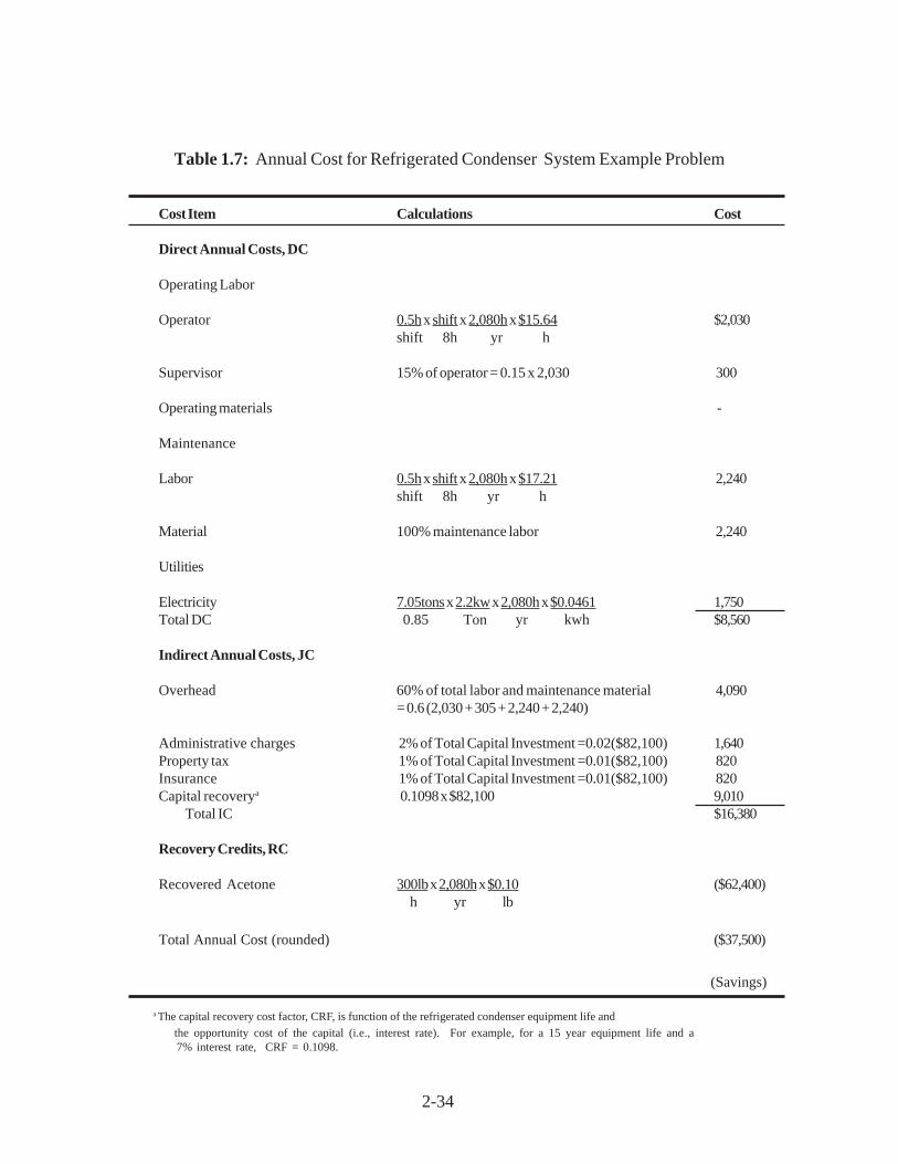
2-34

Table 1.7: Annual Cost for Refrigerated Condenser System Example Problem

Cost Item Calculations Cost

Direct Annual Costs, DC

Operating Labor

Operator 0.5h x shift x 2,080h x $15.64 $2,030shift 8h yr h

Supervisor 15% of operator = 0.15 x 2,030 300

Operating materials -

Maintenance

Labor 0.5h x shift x 2,080h x $17.21 2,240shift 8h yr h

Material 100% maintenance labor 2,240

Utilities

Electricity 7.05tons x 2.2kw x 2,080h x $0.0461 1,750Total DC 0.85 Ton yr kwh $8,560

Indirect Annual Costs, JC

Overhead 60% of total labor and maintenance material 4,090= 0.6 (2,030 + 305 + 2,240 + 2,240)

Administrative charges 2% of Total Capital Investment =0.02($82,100) 1,640Property tax 1% of Total Capital Investment =0.01($82,100) 820Insurance 1% of Total Capital Investment =0.01($82,100) 820Capital recoverya 0.1098 x $82,100 9,010

Total IC $16,380

Recovery Credits, RC

Recovered Acetone 300lb x 2,080h x $0.10 ($62,400) h yr lb

Total Annual Cost (rounded) ($37,500)

(Savings)

a The capital recovery cost factor, CRF, is function of the refrigerated condenser equipment life and the opportunity cost of the capital (i.e., interest rate). For example, for a 15 year equipment life and a 7% interest rate, CRF = 0.1098.

2-35

2.7 Example Problem 2

In this example problem, the alternate design procedure described in Section 2.3.8 isillustrated. The temperature of condensation is given, and the resultant removal efficiency iscalculated. The example stream inlet parameters are identical to Example Problem 1 with theexception that removal efficiency is not specified and the required temperature of condensation isassumed to be 16°F.

2.7.1 Required Information for Design

The first step is to calculate the partial pressure of the VOC at the specified temperature(16°F) using Equation 2.6 to solve for P

VOC:

H = Qloa d g1 4 3

Remember to convert Tcon

to degrees Centigrade, i.e., 16°F = -8.9°C.

Substituting the values for the Antoine equation constants for acetone as listed in Table 2.6:

R = H

= Qloa dg1 2 0 0 0

0 0 1 1 9,

.

PVOC

= 43 mm Hg.

Using Equation 2.24, the removal efficiency is:

Q = Rg .8 3 9

The remainder of the calculations in this problem are identical to those in Example Problem 1.

2.8 Acknowledgments

The authors gratefully acknowledge the following companies for contributing data to thischapter:

• Edwards Engineering (Pompton Plains, NJ)

• Piedmont Engineering (Charlotte, NC)

2-36

• Universal Industrial Refrigeration (Gonzales, LA)

• ITT Standard (Atlanta, GA)

• XChanger (Hopkins, MN)

• Buffalo Tank Co. (Jacksonville, FL)

References

[1] Erikson, D.G., Organic Chemical Manufacturing Volume 5: Adsorption,Condensat ion, and Absorption Devices, U.S. Environmental ProtectionAgency. Research Triangle Park, North Carolina, Publication No. EPA 450/3-80-027, December 1980.

[2] Vatavuk, W.M., and R.B. Neveril, “Estimating Costs of Air Pollution Control Systems: Part XV1. Costs of Refrigeration Systems”, Chemical Engineering, May 16,1983, pp. 95-98.

[3] McCabe, W.L., and J.C. Smith, Unit Operations of Chemical Engineering (ThirdEdition), McGraw-Hill Book Company, New York, 1976.

[4] Perry, R.H. and C.H. Chilton, Eds. Chemical Engineers’ Handbook (Sixth Edi-tion), McGraw-Hill Book Company, New York, 1989.

[5] Kern, D.Q., Process Heat Transfer, McGraw-Hill Book Company, New York,1950

[6] Smith, J.M., and M.C. VanNess, Introduction to Chemical Engineering Thermodynamics (Third Edition), McGraw-Hill Book Company, New York, 1975.

[7] Reid, Robert C., John M. Prausnitz, and Bruce E. Poling, Properties of Gases &Liquids (Fourth Edition), McGraw-Hill Book Company, New York, 1987.

[8] Letter and attachment from Robert V. Sisk. Jr. of Piedmont Engineering, Pineville,North Carolina, to Wiley Barbour of Radian Corporation, Research Triangle Park,North Carolina, January 28, 1991.

[9] Letter and attachment from Waldrop, R., and V. Sardo of Edwards Engineering

2-37

Corp., Pompton Plains, New Jersey, to Wiley Barbour of Radian Corporation,Research Triangle Park, North Carolina, October 1, 1990.

[10] Price, Brian C., “Know the Range and Limitations of Screw Compressors,” Chemi-cal Engineering Progress, 87(2):50-56.

[11] Letter and attachment from Bob Hansek of ITT Corporation, Atlanta, Georgia toWiley Barbour of Radian Corporation, Research Triangle Park, North Carolina,

October 10, 1990.

[12] Letter and attachment from Avery Cooke of Liquid Handling Equipment, Inc., Charlotte, North Carolina to Rich Pelt of Radian Corporation, Research Triangle Park,North Carolina, September 20, 1990.

[13] Letter from Richard Waldrop of Edwards Engineering Corp., Pompton Plains, NewJersey to William Vatavuk, P.E., Durham, North Carolina, August 29, 1988.

2-38

Appendix A

Properties of Selected Compounds

2-39

Table 2.8: Properties of Selected Compounds

CompoundCriticalTemp.a

(�R)

BoilingPoint(�F)

MolecularWeight

(lb/lb-mole)

Heat ofCondensationb

(Btu/lb-mole)

Heat Capacityc

(Btu/lbmole °F)State

Acetone 918 134 58.08 12,510 30.22 Liquid17.90 Gas

Acetylene 555 -119 26.02 7,290 10.50 GasAcrylonitrile - 171 53.06 14,040 15.24 GasAniline 1259 364 93.13 19,160 45.90 Liquid

25.91 GasBenzene 1012 176 78.11 13,230 19.52 LiquidBenzonitrile 1259 376 103.12 19,800 26.07 GasButane 766 31 58.12 9,630 23.29 GasChloroethane 829 54 64.52 10,610 14.97 GasChloroform 966 143 119.39 12,740 15.63 GasChloromethane

750 -12 50.49 9,260 9.74 Gas

Cyclobutane - 55 56.10 10,410 17.26 GasCyclohexane 997 177 84.16 12,890 37.4 Liquid

25.40 GasCyclopentane 921 121 70.13 11,740 30.80 Liquid

19.84 GasCyclopropane 716 -27 42.08 8,630 13.37 GasDiethyl ether 840 94 74.12 11,480 40.8 Liquid

26.89 GasDimethylamine

788 44 45.09 11,390 16.50 Gas

Ethylbenzene 1111 277 106.17 15,300 30.69 GasEthylene oxide 845 51 44.05 10,980 11.54 GasHeptane 973 209 100.12 13,640 53.76 Liquid

39.67 GasHexane 914 156 86.18 12,410 45.2 Liquid

34.20 GasMethanol 923 148 32.04 14,830 19.40 Liquid

10.49 GasOctane 1024 258 114.23 14,810 45.14 GasPentane 846 97 72.15 11,090 28.73 GasToluene 1065 231 92.14 14,270 37.58 Liquid

24.77 Gaso - Xylene 1135 292 106.17 15,840 44.9 Liquid

31.85 Gasm - Xylene 1111 282 106.17 15,640 43.8 Liquid

30.49 Gasp - Xylene 1109 281 106.17 15.480 30.32 Gasa Reprinted with permission from Lange's Handbook of Chemistry (12th edition), Table 9-7.[15]b Reprinted with permission from Lange's Handbook of Chemistry (12th edition), Table 9-4.[15](Measured at boiling point.)c Reprinted with permission from Lanqe's Handbook of Chemistry (12th edition), Table 9-2.[15]

(Measured at 77�F.)

2-40

Table 2.9: Antoine Equation Constants for Selected Compoundsa

Compound

Antoine Equation Constants Valid Temperature Range (�F)

A B C

Acetone 7.117 1210.59555 229.66 Liquid Acetylene 7.100 711.0 253.4 -116 to -98

Acrylonitrile 7.039 1232.53 222.47 -4 to 248

Aniline 7.320 1731.515 206.049 216 to 365

Benzene 6.905 1211.033 220.790 46 to 217

Benzonitrile 6.746 1436.72 181.0 Liquid

Butane 6.809 935.86 238.73 -107 to 66

Chloroethane 6.986 1030.01 238.61 -69 to 54

Chloroethylene 6.891 905.01 239.48 -85 to 9

Chloroform 6.493 929.44 196.03 -31 to 142

Chloromethane 7.0933 948.58 249.34 -103 to 23

Cyanic acid 7.569 1251.86 243.79 -105 to 21

Cyclobutane 6.916 1054.54 241.37 -76 to 54

Cyclohexane 6.841 1201.53 222.65 68 to 178

Cyclopentane 6.887 1124.16 231.36 -40 to 162

Cyclopropane 6.888 856.01 246.50 -130 to -26

Diethyl ether 6.920 1064.07 228.80 -78 to 68

Diethylamine 5.801 583.30 144.1 88 to 142

Dimethylamine 7.082 960.242 221.67 -98 to 44

Dioxane - 1,4 7.432 1554.68 240.34 68 to 221

Ethyl benzene 6.975 1424.255 213.21 79 to 327

Ethylene oxide 7.128 1054.54 2371.76 -56 to 54

Heptane 6.897 1264.90 216.54 28 to 255

Hexane 6.876 1171.17 224.41 -13 to 198

Methanol 7.897 1474.08 229.13 7 to 149

Octane 6.919 1351.99 209.15 66 to 306

Pentane 6.853 1064.84 233.01 -58 to 136

Toluene 6.955 1344.8 219.48 43 to 279

Vinyl acetate 7.210 1296.13 226.66 72 to 162

o - Xylene 6.999 1474.679 213.69 90 to 342

m - Xylene 7.009 1462.266 215.11 82 to 331

p - Xylene 6.991 1453.430 215.31 81 to 331 a Reprinted with permission from Lange's Handbook of Chemistry (12th edition), Table 10-8.[15]

2-41

Appendix B

Documentation forGasoline Vapor Recovery System Cost Data

2-42

As mentioned in Section 2.4.3, vendor cost data were obtained that related the equipmentcost ($) of packaged gasoline vapor recovery systems to the process flow capacity (gal/min). These data needed to be transformed, in order to develop Equation 2.34, which relatesequipment cost ($) to system refrigeration capacity (R, tons), as follows:

ECp = 4,910R + 212,000

To make this transformation, we needed to develop an expression relating flow capacity to refrig-eration capacity. The first step was to determine the inlet partial pressure (P

VOC,in) of the VOC-

gasoline, in this case. As was done in Section 3.1, we assumed that the VOC vapor was saturatedand, thus, in equilibrium with the VOC liquid. This, in turn, meant that we could equate the partialpressure to the vapor pressure. The “model” gasoline had a Reid vapor pressure of 10 and amolecular weight of 66 lb/lb-mole, as shown in Section 4.3 of Compilation of Air PollutantEmission Factors (FPA publication AP-42, Fourth Edition, September 1985). For this gasoline,the following Antoine equation constants were used:

A = 12.5733B = 6386.1

C = 613

These constants were obtained by extrapolating available vapor pressure vs. temperature data forgasoline found in Section 4.3 of AP-42. Upon substi-tuting these constants and an assumed inlettemperature of 77�F (25�C) into the Antoine equation and solving for the inlet partial pressure(P

voc,in) We obtain:

log P AB

T C

= . - .

+

P m m H g

V O C ,inin

V O C ,in

= −+

=

12 57336386 1

25 613

366

If the system operates at atmospheric pressure (760 mm Hg), this partial pressure would corre-spond to a VOC volume fraction in the inlet stream of:

y m m

m m.V O C ,in = =

366

7600 482

2-43

The outlet partial pressure (Pvoc,out

) and volume fraction are calculated in a similar way. Thecondensation (outlet) temperature used in these calcu-lations is -80�F (-62�C), the typical oper-ating Temperature for the gasoline vapor recovery units for which the vendor supplied costs.

log P . .

P . m m H g

V O C ,o u t

V O C ,o u t

= −− +

=

12 57336386 1

62 6139 62

This corresponds to a volume fraction in the outlet stream (yvoc,out

) of:

y. m m

m m.V O C ,ou t = =

9 62

7600 0127

Substitution of PVOC,out

and yVOC,in

into Equation 2.24 yields the condenser removal efficiency (�):

( )( )η =

× −−

=760 0 482 9 62

0 482 760 9 620 986

. .

. ..

The next step in determining the inlet and outlet VOC hourly molar flow rates (Mvoc,in

and Mvoc,out

,respectively). As Equation 2.8 shows, M

voc,in is a function of y

voc,in and the total inlet volumetric

flow rate, Qin, (scfm).

Now, because the gasoline vapor flow rates are typically expressed in gallons/minute, we have toconvert them to scfm. This is done as follows:

Q Q ga l

ft

. ga l. Q sc fmin g g=

× =

m in

1

7 480 134

3

Substituting these variables into Equation 2.8, we obtain:

( ) ( )M. Q

. . Q lb m o le

hrV O C ,in

g

g= =−

0 134

3920 482 60 0 00989

We obtain MVOC,out

from Equation 2.9:

( )M . Q . . Q lb m o les

hrV O C ,o u t g g= − = ×−

−0 00989 1 0 986 1 38 10 4

2-44

And according to Equation 2.10, the amount of gasoline vapor condensed (Mvoc,con

) is thedifference between M

VOC,in and M

voc,out:

M Qlb m oles

hrV O C con g, .=−

0 00975

The final step is to calculate the condenser heat load. This load is a function of the inlet, outlet, andcondensate molar flow rates, the inlet and conden-sation temperatures, the heat capacities of theVOC and air, and the VOC heat of condensation. The VOC heat capacity and heat of conden-sation data used are based on pentane and butane chemical properties, the largest components ofgasoline, and were obtained from CHRIS Hazardous Chemical Data (U.S. Coast Guard, U.S.Department of Transportation, June 1985).

Heat capacities (Btu/Ib-mole-�F):

Cp,VOC

= 26.6C

p,air= 6.95

Heat of condensation of VOC: 9,240 Btu/Ib-mole

Substitution of these data, the molar flow rates, and the temperatures into Equations 2.12, 2.15and 2.16 yields the following enthalpy changes in Btu/hr:

�Hcon

= 130.8Qg

�Huncon

= 0.572Qg

�Hnoncon

= 11.6Qg

The condenser heat load (Hload

) is the sum of these three enthalpy changes (Equation 2.11):

Hload

= 143Qg

The refrigeration capacity (R, tons) is computed from Equation 2.22:

RH

Qloadg= =

12 0000 0119

,.

This last equation relates the refrigeration capacity (tons) to the inlet gaso-line vapor flow rate (gal/min). Solving for Q

g, in terms of R, we obtain:

Qg = 83.9R

2-45

Finally, we substitute this relationship into the equipment cost ($) vs. vapor flow rate (Qg)

correlation, which-was developed from the vendor cost data:

ECp

= 58.5Qg + 212,000

= 58.5(83.9R) + 212,000= 4,910R + 212,000

Note that this last expression is identical to Equation 2.34.

TECHNICAL REPORT DATA(Please read Instructions on reverse before completing)

1. REPORT NO.

452/B-02-0012. 3. RECIPIENT'S ACCESSION NO.

4. TITLE AND SUBTITLE

The EPA Air Pollution Control Cost Manual

5. REPORT DATE

January, 2002 6. PERFORMING ORGANIZATION CODE

7. AUTHOR(S)

Daniel Charles Mussatti

8. PERFORMING ORGANIZATION REPORT NO.

9. PERFORMING ORGANIZATION NAME AND ADDRESS

U.S. Environmental Protection Agency Office of Air Quality Planning and Standards Air Quality Standards and Strategies Division Innovative Strategies and Economics Group Research Triangle Park, NC 27711

10. PROGRAM ELEMENT NO.

11. CONTRACT/GRANT NO.

12. SPONSORING AGENCY NAME AND ADDRESS

Director Office of Air Quality Planning and Standards Office of Air and Radiation U.S. Environmental Protection Agency Research Triangle Park, NC 27711

13. TYPE OF REPORT AND PERIOD COVERED

Final

14. SPONSORING AGENCY CODE

EPA/200/04

15. SUPPLEMENTARY NOTES

Updates and revises EPA 453/b-96-001, OAQPS Control Cost Manual, fifth edition (in English only)

16. ABSTRACT

In Spanish, this document provides a detailed methodology for the proper sizing and costing of numerous airpollution control devices for planning and permitting purposes. Includes costing for volatile organiccompounds (VOCs); particulate matter (PM); oxides of nitrogen (NOx); SO2, SO3, and other acid gasses;and hazardous air pollutants (HAPs).

17. KEY WORDS AND DOCUMENT ANALYSIS

a. DESCRIPTORS b. IDENTIFIERS/OPEN ENDED TERMS c. COSATI Field/Group

EconomicsCostEngineering costSizingEstimationDesign

Air Pollution controlIncineratorsAbsorbersAdsorbersFiltersCondensersElectrostatic PrecipitatorsScrubbers

18. DISTRIBUTION STATEMENT

Release Unlimited

19. SECURITY CLASS (Report)

Unclassified21. NO. OF PAGES

1,400

20. SECURITY CLASS (Page)

Unclassified22. PRICE

EPA Form 2220-1 (Rev. 4-77)EPA Form 2220-1 (Rev. 4-77) PREVIOUS EDITION IS OBSOLETE