SEES2020 Magnetics Notes

Shaun Strong, based on notes by Steve Hearn and Peter Furness

March 29, 2017

Contents

1 Introduction 2

2 Basic Theory and Terminology 32.1 H field, B field, permeability . . . . . . . . . . . . . . . . . . . . . . . . . . . . . . . . . . . 32.2 Units of H, B, µ . . . . . . . . . . . . . . . . . . . . . . . . . . . . . . . . . . . . . . . . . 42.3 Magnetic susceptibility and magnetisation . . . . . . . . . . . . . . . . . . . . . . . . . . . 42.4 Units of susceptibility . . . . . . . . . . . . . . . . . . . . . . . . . . . . . . . . . . . . . . . 52.5 Magnetisation . . . . . . . . . . . . . . . . . . . . . . . . . . . . . . . . . . . . . . . . . . . 52.6 Hysteresis . . . . . . . . . . . . . . . . . . . . . . . . . . . . . . . . . . . . . . . . . . . . . 5

3 Magnetic Properties of Rocks 63.1 Magnetic phenomena . . . . . . . . . . . . . . . . . . . . . . . . . . . . . . . . . . . . . . . 63.2 Susceptibility of common rocks/minerals . . . . . . . . . . . . . . . . . . . . . . . . . . . . 73.3 Remanent Magnetisation . . . . . . . . . . . . . . . . . . . . . . . . . . . . . . . . . . . . . 8

4 The Earths Magnetic Field 94.1 Measured magnetic field . . . . . . . . . . . . . . . . . . . . . . . . . . . . . . . . . . . . . 94.2 Inclination, Declination, Intensity . . . . . . . . . . . . . . . . . . . . . . . . . . . . . . . . 94.3 Magnetic anomalies and latitude . . . . . . . . . . . . . . . . . . . . . . . . . . . . . . . . . 10

4.3.1 Near the equator, where the field is approximately horizontal . . . . . . . . . . . . . 114.3.2 SE Qld. I = −57 . . . . . . . . . . . . . . . . . . . . . . . . . . . . . . . . . . . . . 11

5 Instrumentation(Brief Overview) 125.1 Proton precession magnetometer . . . . . . . . . . . . . . . . . . . . . . . . . . . . . . . . . 125.2 Optically pumped magnetometer . . . . . . . . . . . . . . . . . . . . . . . . . . . . . . . . 13

5.2.1 Zeeman effect . . . . . . . . . . . . . . . . . . . . . . . . . . . . . . . . . . . . . . . 135.3 Vector magnetometer . . . . . . . . . . . . . . . . . . . . . . . . . . . . . . . . . . . . . . . 13

6 Field Procedures (overview) 14

7 Interpretation (overview) 157.1 Qualitative . . . . . . . . . . . . . . . . . . . . . . . . . . . . . . . . . . . . . . . . . . . . 157.2 Quantitative . . . . . . . . . . . . . . . . . . . . . . . . . . . . . . . . . . . . . . . . . . . . 15

1

1 Introduction

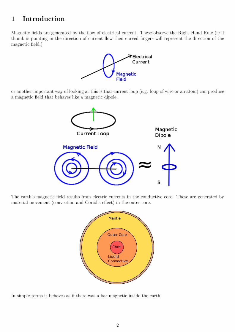
Magnetic fields are generated by the flow of electrical current. These observe the Right Hand Rule (ie ifthumb is pointing in the direction of current flow then curved fingers will represent the direction of themagnetic field.)

or another important way of looking at this is that current loop (e.g. loop of wire or an atom) can producea magnetic field that behaves like a magnetic dipole.

The earth’s magnetic field results from electric currents in the conductive core. These are generated bymaterial movement (convection and Coriolis effect) in the outer core.

In simple terms it behaves as if there was a bar magnetic inside the earth.

2

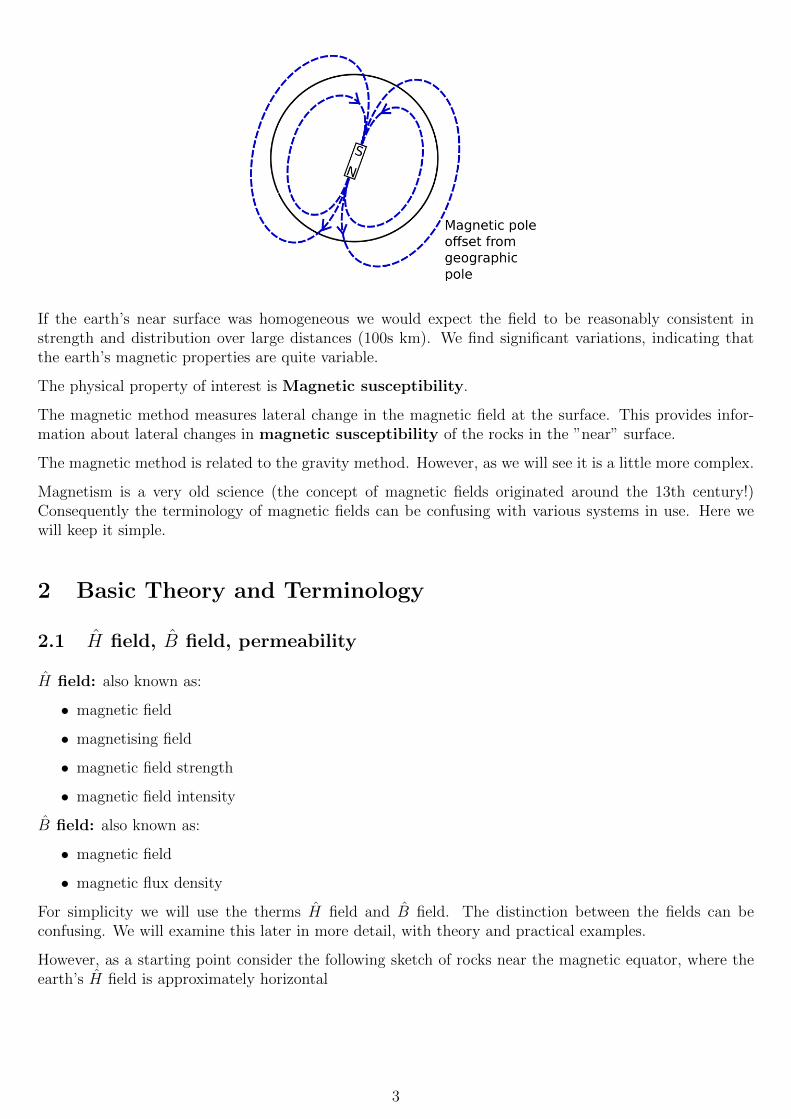
If the earth’s near surface was homogeneous we would expect the field to be reasonably consistent instrength and distribution over large distances (100s km). We find significant variations, indicating thatthe earth’s magnetic properties are quite variable.

The physical property of interest is Magnetic susceptibility.

The magnetic method measures lateral change in the magnetic field at the surface. This provides infor-mation about lateral changes in magnetic susceptibility of the rocks in the ”near” surface.

The magnetic method is related to the gravity method. However, as we will see it is a little more complex.

Magnetism is a very old science (the concept of magnetic fields originated around the 13th century!)Consequently the terminology of magnetic fields can be confusing with various systems in use. Here wewill keep it simple.

2 Basic Theory and Terminology

2.1 H field, B field, permeability

H field: also known as:

• magnetic field

• magnetising field

• magnetic field strength

• magnetic field intensity

B field: also known as:

• magnetic field

• magnetic flux density

For simplicity we will use the therms H field and B field. The distinction between the fields can beconfusing. We will examine this later in more detail, with theory and practical examples.

However, as a starting point consider the following sketch of rocks near the magnetic equator, where theearth’s H field is approximately horizontal

3

The earth’s H field is approximately constant over this whole area. A magnetometer does not measureH, but rather measures a related quality B. The presence of ”iron rich” rocks at location ’2’ results in themeasured B field being different from location ’1’.

What exactly do we mean by ”iron rich”? The technical term is rocks with high magnetic permeability(µ).

Many rocks obey the relationship,

B = µH

2.2 Units of H, B, µ

In SI system the units are:

H → Am−1

B → V sm−2

→ T (Tesla)

µ→ V sm−2

Am−1

→ Ω sm−1

The practical unit of B is nT (10−9 T), also called gamma (γ).

µ in a vacuum is called µo,

µo = 4π ∗ 10−7Ω sm−1

2.3 Magnetic susceptibility and magnetisation

For materials other than a vacuum we can define a relative permeability as

µr =µ

µo

(1)

Consider rocks which obey a linear relationship between B and H. (This is the case for paramagnetic anddiamagnetic materials.)

4

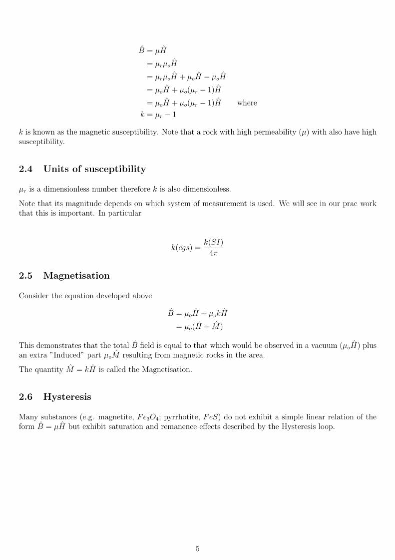
B = µH

= µrµoH

= µrµoH + µoH − µoH

= µoH + µo(µr − 1)H

= µoH + µo(µr − 1)H where

k = µr − 1

k is known as the magnetic susceptibility. Note that a rock with high permeability (µ) with also have highsusceptibility.

2.4 Units of susceptibility

µr is a dimensionless number therefore k is also dimensionless.

Note that its magnitude depends on which system of measurement is used. We will see in our prac workthat this is important. In particular

k(cgs) =k(SI)

4π

2.5 Magnetisation

Consider the equation developed above

B = µoH + µokH

= µo(H + M)

This demonstrates that the total B field is equal to that which would be observed in a vacuum (µoH) plusan extra ”Induced” part µoM resulting from magnetic rocks in the area.

The quantity M = kH is called the Magnetisation.

2.6 Hysteresis

Many substances (e.g. magnetite, Fe3O4; pyrrhotite, FeS) do not exhibit a simple linear relation of theform B = µH but exhibit saturation and remanence effects described by the Hysteresis loop.

5

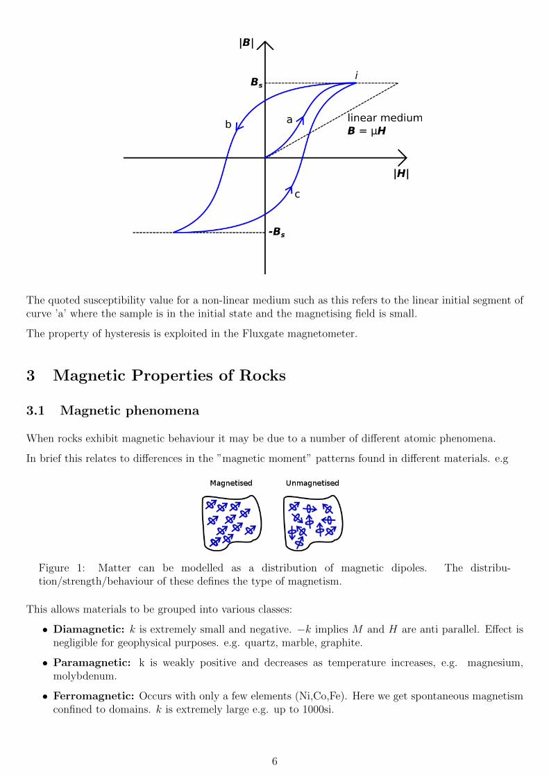
The quoted susceptibility value for a non-linear medium such as this refers to the linear initial segment ofcurve ’a’ where the sample is in the initial state and the magnetising field is small.

The property of hysteresis is exploited in the Fluxgate magnetometer.

3 Magnetic Properties of Rocks

3.1 Magnetic phenomena

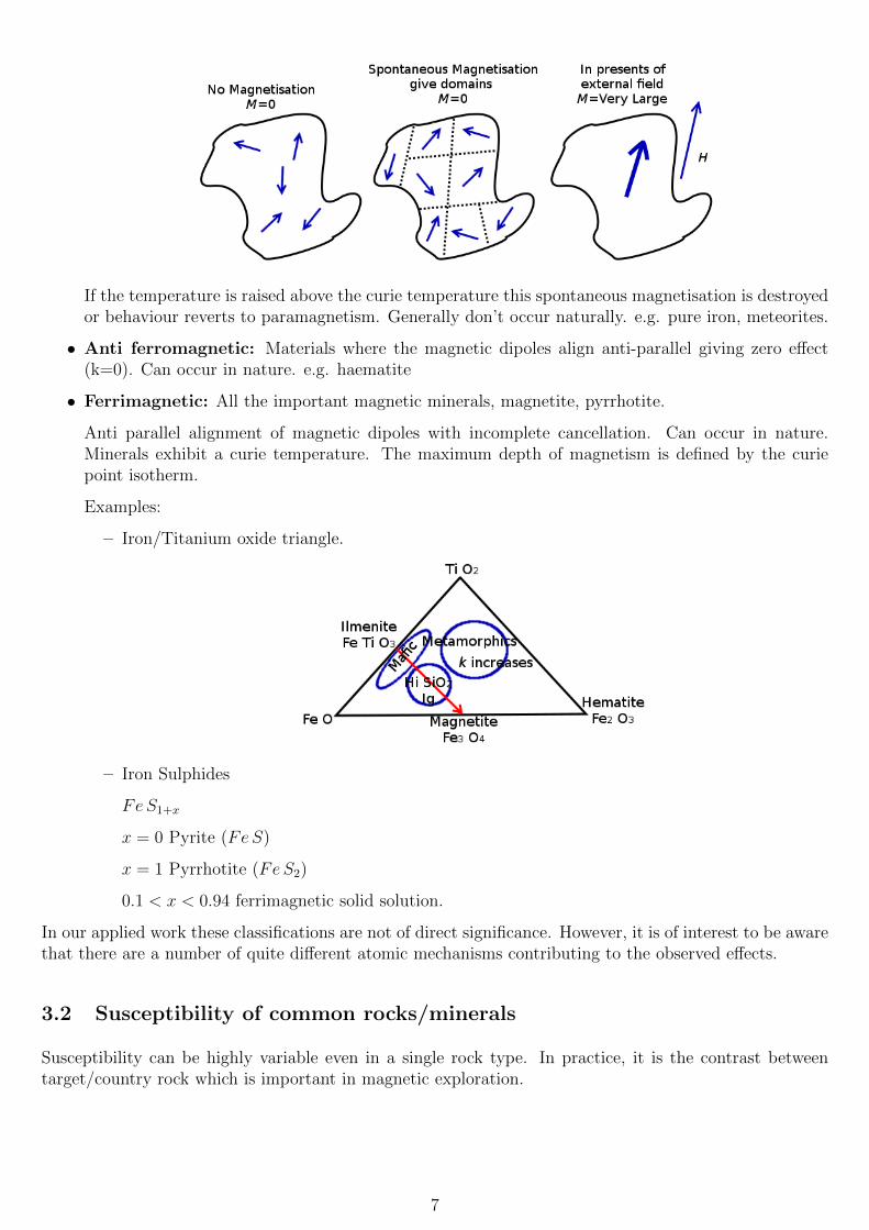
When rocks exhibit magnetic behaviour it may be due to a number of different atomic phenomena.

In brief this relates to differences in the ”magnetic moment” patterns found in different materials. e.g

Figure 1: Matter can be modelled as a distribution of magnetic dipoles. The distribu-tion/strength/behaviour of these defines the type of magnetism.

This allows materials to be grouped into various classes:

• Diamagnetic: k is extremely small and negative. −k implies M and H are anti parallel. Effect isnegligible for geophysical purposes. e.g. quartz, marble, graphite.

• Paramagnetic: k is weakly positive and decreases as temperature increases, e.g. magnesium,molybdenum.

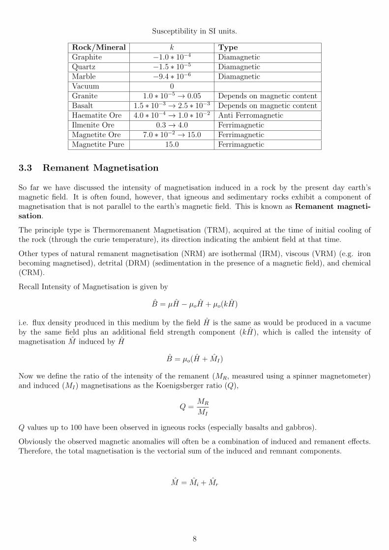
• Ferromagnetic: Occurs with only a few elements (Ni,Co,Fe). Here we get spontaneous magnetismconfined to domains. k is extremely large e.g. up to 1000si.

6

If the temperature is raised above the curie temperature this spontaneous magnetisation is destroyedor behaviour reverts to paramagnetism. Generally don’t occur naturally. e.g. pure iron, meteorites.

• Anti ferromagnetic: Materials where the magnetic dipoles align anti-parallel giving zero effect(k=0). Can occur in nature. e.g. haematite

• Ferrimagnetic: All the important magnetic minerals, magnetite, pyrrhotite.

Anti parallel alignment of magnetic dipoles with incomplete cancellation. Can occur in nature.Minerals exhibit a curie temperature. The maximum depth of magnetism is defined by the curiepoint isotherm.

Examples:

– Iron/Titanium oxide triangle.

– Iron Sulphides

FeS1+x

x = 0 Pyrite (FeS)

x = 1 Pyrrhotite (FeS2)

0.1 < x < 0.94 ferrimagnetic solid solution.

In our applied work these classifications are not of direct significance. However, it is of interest to be awarethat there are a number of quite different atomic mechanisms contributing to the observed effects.

3.2 Susceptibility of common rocks/minerals

Susceptibility can be highly variable even in a single rock type. In practice, it is the contrast betweentarget/country rock which is important in magnetic exploration.

7

Susceptibility in SI units.

Rock/Mineral k TypeGraphite −1.0 ∗ 10−4 DiamagneticQuartz −1.5 ∗ 10−5 DiamagneticMarble −9.4 ∗ 10−6 DiamagneticVacuum 0Granite 1.0 ∗ 10−5 → 0.05 Depends on magnetic contentBasalt 1.5 ∗ 10−3 → 2.5 ∗ 10−3 Depends on magnetic contentHaematite Ore 4.0 ∗ 10−4 → 1.0 ∗ 10−2 Anti FerromagneticIlmenite Ore 0.3→ 4.0 FerrimagneticMagnetite Ore 7.0 ∗ 10−2 → 15.0 FerrimagneticMagnetite Pure 15.0 Ferrimagnetic

3.3 Remanent Magnetisation

So far we have discussed the intensity of magnetisation induced in a rock by the present day earth’smagnetic field. It is often found, however, that igneous and sedimentary rocks exhibit a component ofmagnetisation that is not parallel to the earth’s magnetic field. This is known as Remanent magneti-sation.

The principle type is Thermoremanent Magnetisation (TRM), acquired at the time of initial cooling ofthe rock (through the curie temperature), its direction indicating the ambient field at that time.

Other types of natural remanent magnetisation (NRM) are isothermal (IRM), viscous (VRM) (e.g. ironbecoming magnetised), detrital (DRM) (sedimentation in the presence of a magnetic field), and chemical(CRM).

Recall Intensity of Magnetisation is given by

B = µH − µoH + µo(kH)

i.e. flux density produced in this medium by the field H is the same as would be produced in a vacumeby the same field plus an additional field strength component (kH), which is called the intensity ofmagnetisation M induced by H

B = µo(H + MI)

Now we define the ratio of the intensity of the remanent (MR, measured using a spinner magnetometer)and induced (MI) magnetisations as the Koenigsberger ratio (Q),

Q =MR

MI

Q values up to 100 have been observed in igneous rocks (especially basalts and gabbros).

Obviously the observed magnetic anomalies will often be a combination of induced and remanent effects.Therefore, the total magnetisation is the vectorial sum of the induced and remnant components.

M = Mi + Mr

8

4 The Earths Magnetic Field

4.1 Measured magnetic field

We are looking for variations in the earth’s field. What is its normal state?

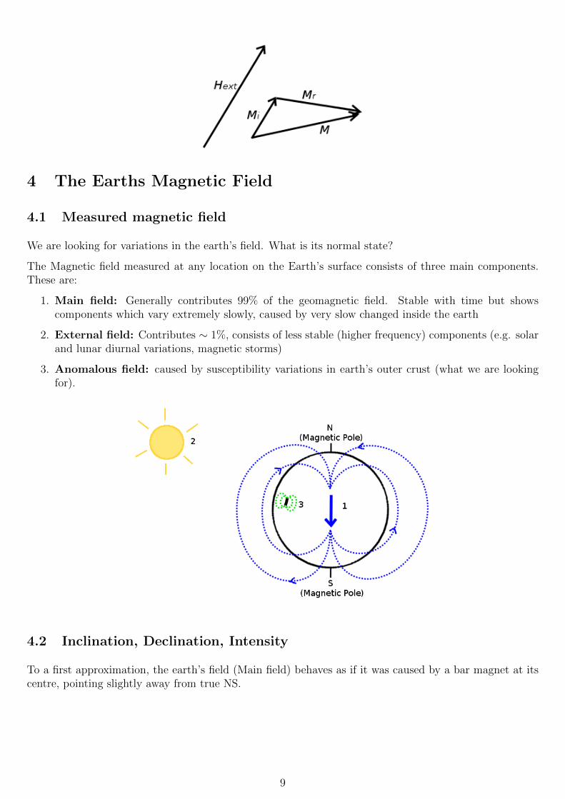
The Magnetic field measured at any location on the Earth’s surface consists of three main components.These are:

1. Main field: Generally contributes 99% of the geomagnetic field. Stable with time but showscomponents which vary extremely slowly, caused by very slow changed inside the earth

2. External field: Contributes ∼ 1%, consists of less stable (higher frequency) components (e.g. solarand lunar diurnal variations, magnetic storms)

3. Anomalous field: caused by susceptibility variations in earth’s outer crust (what we are lookingfor).

4.2 Inclination, Declination, Intensity

To a first approximation, the earth’s field (Main field) behaves as if it was caused by a bar magnet at itscentre, pointing slightly away from true NS.

9

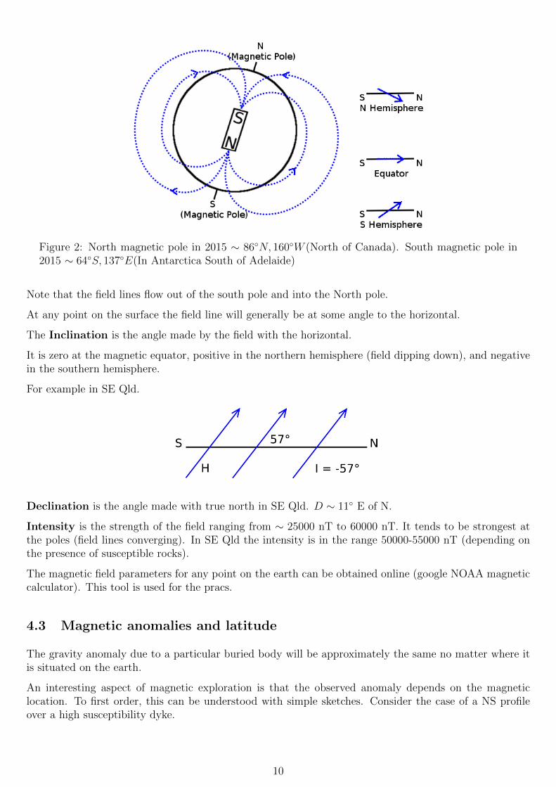
Figure 2: North magnetic pole in 2015 ∼ 86N, 160W (North of Canada). South magnetic pole in2015 ∼ 64S, 137E(In Antarctica South of Adelaide)

Note that the field lines flow out of the south pole and into the North pole.

At any point on the surface the field line will generally be at some angle to the horizontal.

The Inclination is the angle made by the field with the horizontal.

It is zero at the magnetic equator, positive in the northern hemisphere (field dipping down), and negativein the southern hemisphere.

For example in SE Qld.

Declination is the angle made with true north in SE Qld. D ∼ 11 E of N.

Intensity is the strength of the field ranging from ∼ 25000 nT to 60000 nT. It tends to be strongest atthe poles (field lines converging). In SE Qld the intensity is in the range 50000-55000 nT (depending onthe presence of susceptible rocks).

The magnetic field parameters for any point on the earth can be obtained online (google NOAA magneticcalculator). This tool is used for the pracs.

4.3 Magnetic anomalies and latitude

The gravity anomaly due to a particular buried body will be approximately the same no matter where itis situated on the earth.

An interesting aspect of magnetic exploration is that the observed anomaly depends on the magneticlocation. To first order, this can be understood with simple sketches. Consider the case of a NS profileover a high susceptibility dyke.

10

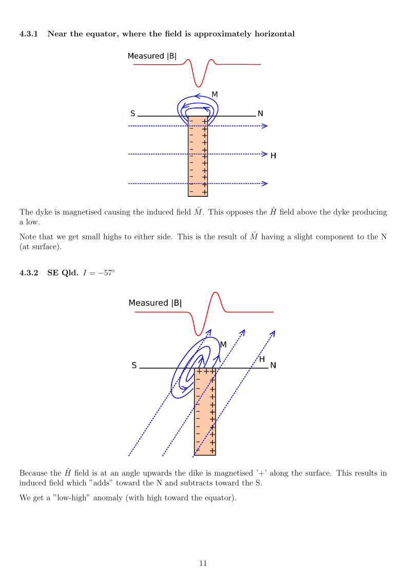
4.3.1 Near the equator, where the field is approximately horizontal

The dyke is magnetised causing the induced field M . This opposes the H field above the dyke producinga low.

Note that we get small highs to either side. This is the result of M having a slight component to the N(at surface).

4.3.2 SE Qld. I = −57

Because the H field is at an angle upwards the dike is magnetised ’+’ along the surface. This results ininduced field which ”adds” toward the N and subtracts toward the S.

We get a ”low-high” anomaly (with high toward the equator).

11

5 Instrumentation(Brief Overview)

5.1 Proton precession magnetometer

(proton free-precession magnetometer)

Utilises the property of nuclear magnetic resonance (NMR).

Basically

Every proton because it is spinning and is charged has an angular momentum J and a magnetic momentm, the two vectors being related via

m = γ J

where γ is the gyromagnetic ratio, accurately known for protons.

In a bottle of H2O sitting in the undisturbed earth’s fields, the magnetic moment vectors of the protonswill align the themselves parallel to the earth’s field.

If a strong auxiliary field (via a coil wrap) is then applied in some other direction the magnetic momentvectors will gradually align themselves to the direction of the resultant (∼ 5 sec).

If the artificial field is then removed rapidly, the earth’s field imposes a torque on the spinning protonscausing them to precess about the direction of the earth’s field (like an unstable spinning top).

The frequency of the precession is ω = γ|B|, which can be detected as the frequency of a small voltagegenerated in the can. Since the gyromagnetic ratio is known we can derived the flux density |B|. i.e. Thegyromagnetic ratio for a proton is γP = 2.675 ∗ 108 SI therefore

|B| = 2π

γPf

The precession damps out and protons return to the ambient orientation.

Note that the precession frequency doesn’t depend on the angle between B and m. That is, This is a totalfield instrument which doesn’t require levelling, and is suitable to airbourne or shipbourne use

12

5.2 Optically pumped magnetometer

caesium-vapour magnetometer

rubidium-vapour magnetometer

Based on the principle of quantum mechanics.

In an atom, electrons can only exist in certain configurations. Electrons can make transitions between theseallowed energy levels. If energy is absorbed they move to a higher energy level and if they move to a lowerlevel energy is released (usually as photons). There is a relationship between energy released/absorbed(∆E) and the frequency (f) of the photons,

∆E = hf

The state of an electron in an atom is described by 4 quantum numbers:

• n, principal quantum number.

• l, azimuthal quantum number.

• m, magnetic quantum number.

• spin quantum number.

5.2.1 Zeeman effect

In an optically pumped magnetometer these principles are applied to cesium/rubidium atoms in a smallcontainer. The frequency of energy associated with variations is measured. This yields ∆E values whichin turn allows an estimate of the ambient magnetic field B.

Sensitivity is ∼ 0.01 nT

5.3 Vector magnetometer

Very commonly, magnetic surveys measure the magnitude of the total field resulting from the interactionof the earth’s ambient field and the induced magnetisation in rocks.

The proton-precession and optically-pumped magnetometers are both scalar instruments measuring totalfield.

13

It is sometimes of interest to measure the earth’s field in magnitude and direction. This is a vectormeasurement.

One example of a vector magnetometer is the Flux Gate magnetometer.

As noted above, this uses the idea of hysteresis.

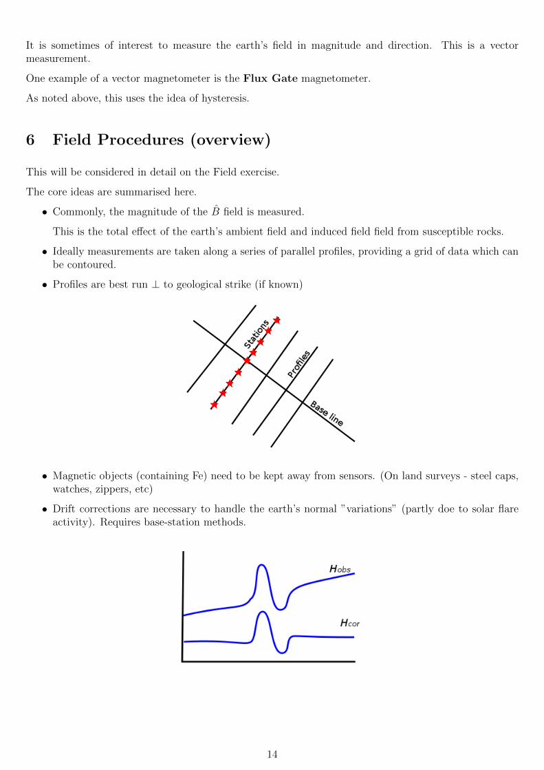
6 Field Procedures (overview)

This will be considered in detail on the Field exercise.

The core ideas are summarised here.

• Commonly, the magnitude of the B field is measured.

This is the total effect of the earth’s ambient field and induced field field from susceptible rocks.

• Ideally measurements are taken along a series of parallel profiles, providing a grid of data which canbe contoured.

• Profiles are best run ⊥ to geological strike (if known)

• Magnetic objects (containing Fe) need to be kept away from sensors. (On land surveys - steel caps,watches, zippers, etc)

• Drift corrections are necessary to handle the earth’s normal ”variations” (partly doe to solar flareactivity). Requires base-station methods.

14

7 Interpretation (overview)

7.1 Qualitative

• Work from a contour map of |B| or BZ (in nT).

• generally interested in any variations or anomalies relative to a general low-relief background. e.g

– Closed highs or lows indicates ore bodies, intrusions.

– Areas of high gradient indicate rapid lateral change from one material to another.

– Long narrow highs/lows may indicate dykes, tectonic shear zones, elongated ore bodies.

– Dislocations in contours indicate faulting.

– High intensity areas of considerable extent may indicate basalt flows.

• Obviously interpretation must be done in conjunction with geological information.

7.2 Quantitative

• Most quantitative interpretation is done by assuming some geology model, computing the theoreticalmagnetic flux density at the observed points, compare and iterate.

• Normally done on selected profiles i.e. 2-D modelling.

• Non uniqueness of solution, requires further geological input to arrive at a valid model.

• Theoretical calculations of magnetic flux density due to various subsurface distributions of materialtake as a starting point the Poisson equation.

O2φ = div M where,

M = intensity of magnetisation

φ = scalar magnetic potential where,

H = −Oφ

Note that:

O2φ =δ2φ

δx2+δ2φ

δy2+δ2φ

δz2

Oφ =δφ

δxi+

δφ

δyj +

δφ

δzk

div M =δMx

δx+δMy

δy+δMz

δz

• The calculation of the theoretical anomaly of an arbitrary distribution of magnetic material is rea-sonably complicated although it can be handled numerically. However, reasonably elegant analyticalsolutions can be obtained for simple structures, e.g. sphere, thin sheet, thick sheet, prism.

15