An Eponymous Dictionary of Economics

An Eponymous Dictionaryof EconomicsA Guide to Laws and Theorems Named after Economists

Edited by

Julio SeguraProfessor of Economic Theory, Universidad Complutense, Madrid, Spain,

and

Carlos Rodríguez BraunProfessor of History of Economic Thought, Universidad Complutense,Madrid, Spain

Edward ElgarCheltenham, UK • Northampton, MA, USA

© Carlos Rodríguez Braun and Julio Segura 2004

All rights reserved. No part of this publication may be reproduced, stored in a retrieval system or transmitted in any form or by any means, electronic, mechanical or photocopying, recording, or otherwise without the prior permission of the publisher.

Published byEdward Elgar Publishing LimitedGlensanda HouseMontpellier ParadeCheltenhamGlos GL50 1UAUK

Edward Elgar Publishing, Inc.136 West StreetSuite 202NorthamptonMassachusetts 01060USA

A catalogue record for this bookis available from the British Library

ISBN 1 84376 029 0 (cased)

Typeset by Cambrian Typesetters, Frimley, SurreyPrinted and bound in Great Britain by MPG Books Ltd, Bodmin, Cornwall

Contents

List of contributors and their entries xiiiPreface xxvii

Adam Smith problem 1Adam Smith’s invisible hand 1Aitken’s theorem 3Akerlof’s ‘lemons’ 3Allais paradox 4Areeda–Turner predation rule 4Arrow’s impossibility theorem 6Arrow’s learning by doing 8Arrow–Debreu general equilibrium model 9Arrow–Pratt’s measure of risk aversion 10Atkinson’s index 11Averch–Johnson effect 12

Babbage’s principle 13Bagehot’s principle 13Balassa–Samuelson effect 14Banach’s contractive mapping principle 14Baumol’s contestable markets 15Baumol’s disease 16Baumol–Tobin transactions demand for cash 17Bayes’s theorem 18Bayesian–Nash equilibrium 19Becher’s principle 20Becker’s time allocation model 21Bellman’s principle of optimality and equations 23Bergson’s social indifference curve 23Bernoulli’s paradox 24Berry–Levinsohn–Pakes algorithm 25Bertrand competition model 25Beveridge–Nelson decomposition 27Black–Scholes model 28Bonferroni bound 29Boolean algebras 30Borda’s rule 30Bowley’s law 31Box–Cox transformation 31Box–Jenkins analysis 32Brouwer fixed point theorem 34

v

Buchanan’s clubs theory 34Buridan’s ass 35

Cagan’s hyperinflation model 36Cairnes–Haberler model 36Cantillon effect 37Cantor’s nested intervals theorem 38Cass–Koopmans criterion 38Cauchy distribution 39Cauchy’s sequence 39Cauchy–Schwarz inequality 40Chamberlin’s oligopoly model 41Chipman–Moore–Samuelson compensation criterion 42Chow’s test 43Clark problem 43Clark–Fisher hypothesis 44Clark–Knight paradigm 44Coase conjecture 45Coase theorem 46Cobb–Douglas function 47Cochrane–Orcutt procedure 48Condorcet’s criterion 49Cournot aggregation condition 50Cournot’s oligopoly model 51Cowles Commission 52Cox’s test 53

Davenant–King law of demand 54Díaz–Alejandro effect 54Dickey–Fuller test 55Director’s law 56Divisia index 57Dixit–Stiglitz monopolistic competition model 58Dorfman–Steiner condition 60Duesenberry demonstration effect 60Durbin–Watson statistic 61Durbin–Wu–Hausman test 62

Edgeworth box 63Edgeworth expansion 65Edgeworth oligopoly model 66Edgeworth taxation paradox 67Ellsberg paradox 68Engel aggregation condition 68Engel curve 69Engel’s law 71

vi Contents

Engle–Granger method 72Euclidean spaces 72Euler’s theorem and equations 73

Farrell’s technical efficiency measurement 75Faustmann–Ohlin theorem 75Fisher effect 76Fisher–Shiller expectations hypothesis 77Fourier transform 77Friedman’s rule for monetary policy 79Friedman–Savage hypothesis 80Fullarton’s principle 81Fullerton–King’s effective marginal tax rate 82

Gale–Nikaido theorem 83Gaussian distribution 84Gauss–Markov theorem 86Genberg–Zecher criterion 87Gerschenkron’s growth hypothesis 87Gibbard–Satterthwaite theorem 88Gibbs sampling 89Gibrat’s law 90Gibson’s paradox 90Giffen goods 91Gini’s coefficient 91Goodhart’s law 92Gorman’s polar form 92Gossen’s laws 93Graham’s demand 94Graham’s paradox 95Granger’s causality test 96Gresham’s law 97Gresham’s law in politics 98

Haavelmo balanced budget theorem 99Hamiltonian function and Hamilton–Jacobi equations 100Hansen–Perlof effect 101Harberger’s triangle 101Harris–Todaro model 102Harrod’s technical progress 103Harrod–Domar model 104Harsanyi’s equiprobability model 105Hausman’s test 105Hawkins–Simon theorem 106Hayekian triangle 107Heckman’s two-step method 108

Contents vii

Heckscher–Ohlin theorem 109Herfindahl–Hirschman index 111Hermann–Schmoller definition 111Hessian matrix and determinant 112Hicks compensation criterion 113Hicks composite commodities 113Hicks’s technical progress 113Hicksian demand 114Hicksian perfect stability 115Hicks–Hansen model 116Hodrick–Prescott decomposition 118Hotelling’s model of spatial competition 118Hotelling’s T2 statistic 119Hotelling’s theorem 120Hume’s fork 121Hume’s law 121

Itô’s lemma 123

Jarque–Bera test 125Johansen’s procedure 125Jones’s magnification effect 126Juglar cycle 126

Kakutani’s fixed point theorem 128Kakwani index 128Kalai–Smorodinsky bargaining solution 129Kaldor compensation criterion 129Kaldor paradox 130Kaldor’s growth laws 131Kaldor–Meade expenditure tax 131Kalman filter 132Kelvin’s dictum 133Keynes effect 134Keynes’s demand for money 134Keynes’s plan 136Kitchin cycle 137Kolmogorov’s large numbers law 137Kolmogorov–Smirnov test 138Kondratieff long waves 139Koopman’s efficiency criterion 140Kuhn–Tucker theorem 140Kuznets’s curve 141Kuznets’s swings 142

Laffer’s curve 143Lagrange multipliers 143

viii Contents

Lagrange multiplier test 144Lancaster’s characteristics 146Lancaster–Lipsey’s second best 146Lange–Lerner mechanism 147Laspeyres index 148Lauderdale’s paradox 148Learned Hand formula 149Lebesgue’s measure and integral 149LeChatelier principle 150Ledyard–Clark–Groves mechanism 151Leontief model 152Leontief paradox 153Lerner index 154Lindahl–Samuelson public goods 155Ljung–Box statistics 156Longfield paradox 157Lorenz’s curve 158Lucas critique 158Lyapunov’s central limit theorem 159Lyapunov stability 159

Mann–Wald’s theorem 161Markov chain model 161Markov switching autoregressive model 162Markowitz portfolio selection model 163Marshall’s external economies 164Marshall’s stability 165Marshall’s symmetallism 166Marshallian demand 166Marshall–Lerner condition 167Maskin mechanism 168Minkowski’s theorem 169Modigliani–Miller theorem 170Montaigne dogma 171Moore’s law 172Mundell–Fleming model 172Musgrave’s three branches of the budget 173Muth’s rational expectations 175Myerson revelation principle 176

Nash bargaining solution 178Nash equilibrium 179Negishi’s stability without recontracting 181von Neumann’s growth model 182von Neumann–Morgenstern expected utility theorem 183von Neumann–Morgenstern stable set 185

Contents ix

Newton–Raphson method 185Neyman–Fisher theorem 186Neyman–Pearson test 187

Occam’s razor 189Okun’s law and gap 189

Paasche index 192Palgrave’s dictionaries 192Palmer’s rule 193Pareto distribution 194Pareto efficiency 194Pasinetti’s paradox 195Patman effect 197Peacock–Wiseman’s displacement effect 197Pearson chi-squared statistics 198Peel’s law 199Perron–Frobenius theorem 199Phillips curve 200Phillips–Perron test 201Pigou effect 203Pigou tax 204Pigou–Dalton progressive transfers 204Poisson’s distribution 205Poisson process 206Pontryagin’s maximun principle 206Ponzi schemes 207Prebisch–Singer hypothesis 208

Radner’s turnpike property 210Ramsey model and rule 211Ramsey’s inverse elasticity rule 212Rao–Blackwell’s theorem 213Rawls’s justice criterion 213Reynolds–Smolensky index 214Ricardian equivalence 215Ricardian vice 216Ricardo effect 217Ricardo’s comparative costs 218Ricardo–Viner model 219Robinson–Metzler condition 220Rostow’s model 220Roy’s identity 222Rubinstein’s model 222Rybczynski theorem 223

x Contents

Samuelson condition 225Sard’s theorem 225Sargan test 226Sargant effect 227Say’s law 227Schmeidler’s lemma 229Schumpeter’s vision 230Schumpeterian entrepreneur 230Schwarz criterion 231Scitovsky’s community indifference curve 232Scitovsky’s compensation criterion 232Selten paradox 233Senior’s last hour 234Shapley value 235Shapley–Folkman theorem 236Sharpe’s ratio 236Shephard’s lemma 237Simon’s income tax base 238Slutksky equation 238Slutsky–Yule effect 240Snedecor F-distribution 241Solow’s growth model and residual 242Sonnenschein–Mantel–Debreu theorem 244Spencer’s law 244Sperner’s lemma 245Sraffa’s model 245Stackelberg’s oligopoly model 246Stigler’s law of eponymy 247Stolper–Samuelson theorem 248Student t-distribution 248Suits index 250Swan’s model 251

Tanzi–Olivera effect 252Taylor rule 252Taylor’s theorem 253Tchébichef’s inequality 254Theil index 254Thünen’s formula 255Tiebout’s voting with the feet process 256Tinbergen’s rule 257Tobin’s q 257Tobin’s tax 258Tocqueville’s cross 260Tullock’s trapezoid 261Turgot–Smith theorem 262

Contents xi

Veblen effect good 264Verdoorn’s law 264Vickrey auction 265

Wagner’s law 266Wald test 266Walras’s auctioneer and tâtonnement 268Walras’s law 268Weber–Fechner law 269Weibull distribution 270Weierstrass extreme value theorem 270White test 271Wicksell effect 271Wicksell’s benefit principle for the distribution of tax burden 273Wicksell’s cumulative process 274Wiener process 275Wiener–Khintchine theorem 276Wieser’s law 276Williams’s fair innings argument 277Wold’s decomposition 277

Zellner estimator 279

xii Contents

Contributors and their entries

Albarrán, Pedro, Universidad Carlos III, Madrid, SpainPigou tax

Albert López-Ibor, Rocío, Universidad Complutense, Madrid, SpainLearned Hand formula

Albi, Emilio, Universidad Complutense, Madrid, SpainSimons’s income tax base

Almenar, Salvador, Universidad de Valencia, Valencia, SpainEngel’s law

Almodovar, António, Universidade do Porto, Porto, PortugalWeber–Fechner law

Alonso, Aurora, Universidad del País Vasco-EHU, Bilbao, SpainLucas critique

Alonso Neira, Miguel Ángel, Universidad Rey Juan Carlos, Madrid, SpainHayekian triangle

Andrés, Javier, Universidad de Valencia, Valencia, SpainPigou effect

Aparicio-Acosta, Felipe M., Universidad Carlos III, Madrid, SpainFourier transform

Aragonés, Enriqueta, Universitat Autònoma de Barcelona, Barcelona, SpainRawls justice criterion

Arellano, Manuel, CEMFI, Madrid, SpainLagrange multiplier test

Argemí, Lluís, Universitat de Barcelona, Barcelona, SpainGossen’s laws

Arruñada, Benito, Universitat Pompeu Fabra, Barcelona, SpainBaumol’s disease

Artés Caselles, Joaquín, Universidad Complutense, Madrid, SpainLeontief paradox

Astigarraga, Jesús, Universidad de Deusto, Bilbao, SpainPalgrave’s dictionaries

Avedillo, Milagros, Comisión Nacional de Energía, Madrid, SpainDivisia index

Ayala, Luis, Universidad Rey Juan Carlos, Madrid, SpainAtkinson index

xiii

Ayuso, Juan, Banco de España, Madrid, SpainAllais paradox; Ellsberg paradox

Aznar, Antonio, Universidad de Zaragoza, Zaragoza, SpainDurbin–Wu–Hausman test

Bacaria, Jordi, Universitat Autònoma de Barcelona, Barcelona, SpainBuchanan’s clubs theory

Badenes Plá, Nuria, Universidad Complutense, Madrid, SpainKaldor–Meade expenditure tax; Tiebout’s voting with the feet process; Tullock’s trapezoid

Barberá, Salvador, Universitat Autònoma de Barcelona, Barcelona, SpainArrow’s impossibility theorem

Bel, Germà, Universitat de Barcelona, Barcelona, SpainClark problem; Clark–Knight paradigm

Bentolila, Samuel, CEMFI, Madrid, SpainHicks–Hansen model

Bergantiños, Gustavo, Universidad de Vigo, Vigo, Pontevedra, SpainBrouwer fixed point theorem; Kakutani’s fixed point theorem

Berganza, Juan Carlos, Banco de España, Madrid, SpainLerner index

Berrendero, José R., Universidad Autónoma, Madrid, SpainKolmogorov–Smirnov test

Blanco González, María, Universidad San Pablo CEU, Madrid, SpainCowles Commission

Bobadilla, Gabriel F., Omega-Capital, Madrid, SpainMarkowitz portfolio selection model; Fisher–Shiller expectations hypothesis

Bolado, Elsa, Universitat de Barcelona, Barcelona, SpainKeynes effect

Borrell, Joan-Ramon, Universitat de Barcelona, Barcelona, SpainBerry–Levinsohn–Pakes algorithm

Bover, Olympia, Banco de España, Madrid, SpainGaussian distribution

Bru, Segundo, Universidad de Valencia, Valencia, SpainSenior’s last hour

Burguet, Roberto, Universitat Autònoma de Barcelona, Barcelona, SpainWalras’s auctioneer and tâtonnement

Cabrillo, Francisco, Universidad Complutense, Madrid, SpainCoase theorem

Calderón Cuadrado, Reyes, Universidad de Navarra, Pamplona, SpainHermann–Schmoller definition

xiv Contributors and their entries

Callealta, Francisco J., Universidad de Alcalá de Henares, Alcalá de Henares, Madrid,SpainNeyman–Fisher theorem

Calsamiglia, Xavier, Universitat Pompeu Fabra, Barcelona, SpainGale–Nikaido theorem

Calzada, Joan, Universitat de Barcelona, Barcelona, SpainStolper–Samuelson theorem

Candeal, Jan Carlos, Universidad de Zaragoza, Zaragoza, SpainCantor’s nested intervals theorem; Cauchy’s sequence

Carbajo, Alfonso, Confederación Española de Cajas de Ahorro, Madrid, SpainDirector’s law

Cardoso, José Luís, Universidad Técnica de Lisboa, Lisboa, PortugalGresham’s law

Carnero, M. Angeles, Universidad Carlos III, Madrid, SpainMann–Wald’s theorem

Carrasco, Nicolás, Universidad Carlos III, Madrid, SpainCox’s test; White test

Carrasco, Raquel, Universidad Carlos III, Madrid, SpainCournot aggregation condition; Engel aggregation condition

Carrera, Carmen, Universidad Complutense, Madrid, SpainSlutsky equation

Caruana, Guillermo, CEMFI, Madrid, SpainHicks composite commodities

Castillo, Ignacio del, Ministerio de Hacienda, Madrid, SpainFullarton’s principle

Castillo Franquet, Joan, Universitat Autònoma de Barcelona, Barcelona, SpainTchébichef’s inequality

Castro, Ana Esther, Universidad de Vigo, Vigo, Pontevedra, SpainPonzi schemes

Cerdá, Emilio, Universidad Complutense, Madrid, SpainBellman’s principle of optimality and equations; Euler’s theorem and equations

Comín, Diego, New York University, New York, USAHarrod–Domar model

Corchón, Luis, Universidad Carlos III, Madrid, SpainMaskin mechanism

Costas, Antón, Universitat de Barcelona, Barcelona, SpainPalmer’s Rule; Peel’s Law

Contributors and their entries xv

Díaz-Emparanza, Ignacio, Instituto de Economía Aplicada, Universidad del País Vasco-EHU, Bilbao, SpainCochrane–Orcutt procedure

Dolado, Juan J., Universidad Carlos III, Madrid, SpainBonferroni bound; Markov switching autoregressive model

Domenech, Rafael, Universidad de Valencia, Valencia, SpainSolow’s growth model and residual

Echevarría, Cruz Angel, Universidad del País Vasco-EHU, Bilbao, SpainOkun’s law and gap

Escribano, Alvaro, Universidad Carlos III, Madrid, SpainEngle–Granger method; Hodrick–Prescott decomposition

Espasa, Antoni, Universidad Carlos III, Madrid, SpainBox–Jenkins analysis

Espiga, David, La Caixa-S.I. Gestión Global de Riesgos, Barcelona, SpainEdgeworth oligopoly model

Esteban, Joan M., Universitat Autònoma de Barcelona, Barcelona, SpainPigou–Dalton progressive transfers

Estrada, Angel, Banco de España, Madrid, SpainHarrod’s technical progress; Hicks’s technical progress

Etxebarria Zubeldía, Gorka, Deloitte & Touche, Madrid, SpainMontaigne dogma

Fariñas, José C., Universidad Complutense, Madrid, SpainDorfman–Steiner condition

Febrero, Ramón, Universidad Complutense, Madrid, SpainBecker’s time allocation model

Fernández, José L., Universidad Autónoma, Madrid, SpainCauchy–Schwarz inequality; Itô’s lemma

Fernández Delgado, Rogelio, Universidad Rey Juan Carlos, Madrid, SpainPatman effect

Fernández-Macho, F. Javier, Universidad del País Vasco-EHU, Bilbao, SpainSlutsky–Yule effect

Ferreira, Eva, Universidad del País Vasco-EHU, Bilbao, SpainBlack–Scholes model; Pareto distribution; Sharpe’s ratio

Flores Parra, Jordi, Servicio de Estudios de Caja Madrid, Madrid, Spain and UniversidadCarlos III, Madrid, SpainSamuelson’s condition

Franco, Yanna G., Universidad Complutense, Madrid, SpainCairnes–Haberler model; Ricardo–Viner model

xvi Contributors and their entries

Freire Rubio, Mª Teresa, Escuela Superior de Gestión Comercial y Marketing, Madrid,SpainLange–Lerner mechanism

Freixas, Xavier, Universitat Pompeu Fabra, Barcelona, Spain and CEPRFriedman-Savage hypothesis

Frutos de, M. Angeles, Universidad Carlos III, Madrid, SpainHotelling’s model of spatial competition

Fuente de la, Angel, Universitat Autònoma de Barcelona, Barcelona, SpainSwan’s model

Gallastegui, Carmen, Universidad del País Vasco-EHU, Bilbao, SpainPhillip’s curve

Gallego, Elena, Universidad Complutense, Madrid, SpainRobinson-Metzler condition

García, Jaume, Universitat Pompeu Fabra, Barcelona, SpainHeckman’s two-step method

García-Bermejo, Juan C., Universidad Autónoma, Madrid, SpainHarsanyi’s equiprobability model

García-Jurado, Ignacio, Universidad de Santiago de Compostela, Santiago de Compostela,A Coruña, SpainSelten paradox

García Ferrer, Antonio, Universidad Autónoma, Madrid, SpainZellner estimator

García Lapresta, José Luis, Universidad de Valladolid, Valladolid, SpainBolean algebras; Taylor’s theorem

García Pérez, José Ignacio, Fundación CENTRA, Sevilla, SpainScitovsky’s compensation criterion

García-Ruiz, José L., Universidad Complutense, Madrid, SpainHarris–Todaro model; Prebisch–Singer hypothesis

Gimeno, Juan A., Universidad Nacional de Educación a Distancia, Madrid, SpainPeacock–Wiseman’s displacement effect; Wagner’s law

Girón, F. Javier, Universidad de Málaga, Málaga, SpainGauss–Markov theorem

Gómez Rivas, Léon, Universidad Europea, Madrid, SpainLongfield’s paradox

Graffe, Fritz, Universidad del País Vasco-EHU, Bilbao, SpainLeontief model

Grifell-Tatjé, E., Universitat Autònoma de Barcelona, Barcelona, SpainFarrell’s technical efficiency measurement

Contributors and their entries xvii

Guisán, M. Cármen, Universidad de Santiago de Compostela, Santiago de Compostela, ACoruña, SpainChow’s test; Granger’s causality test

Herce, José A., Universidad Complutense, Madrid, SpainCass–Koopmans criterion; Koopmans’s efficiency criterion

Herguera, Iñigo, Universidad Complutense, Madrid, SpainGorman’s polar form

Hernández Andreu, Juan, Universidad Complutense, Madrid, SpainJuglar cycle; Kitchin cycle; Kondratieff long waves

Herrero, Cármen, Universidad de Alicante, Alicante, SpainPerron–Frobenius theorem

Herrero, Teresa, Confederación Española de Cajas de Ahorro, Madrid, SpainHeckscher–Ohlin theorem; Rybczynski theorem

Hervés-Beloso, Carlos, Universidad de Vigo, Vigo, Pontevedra, SpainSard’s theorem

Hoyo, Juan del, Universidad Autónoma, Madrid, SpainBox–Cox transformation

Huergo, Elena, Universidad Complutense, Madrid, SpainStackelberg’s oligopoly model

Huerta de Soto, Jesús, Universidad Rey Juan Carlos, Madrid, SpainRicardo effect

Ibarrola, Pilar, Universidad Complutense, Madrid, SpainLjung–Box statistics

Iglesia, Jesús de la, Universidad Complutense, Madrid, SpainTocqueville’s cross

de la Iglesia Villasol, Mª Covadonga, Universidad Complutense, Madrid, SpainHotelling’s theorem

Iñarra, Elena, Universidad deli País Vasco-EHU, Bilbao, Spainvon Neumann–Morgenstern stable set

Induraín, Esteban, Universidad Pública de Navarra, Pamplona, SpainHawkins–Simon theorem; Weierstrass extreme value theorem

Jimeno, Juan F., Universidad de Alcalá de Henares, Alcalá de Henares, Madrid, SpainRamsey model and rule

Justel, Ana, Universidad Autónoma, Madrid, SpainGibbs sampling

Lafuente, Alberto, Universidad de Zaragoza, Zaragoza, SpainHerfindahl–Hirschman index

xviii Contributors and their entries

Lasheras, Miguel A., Grupo CIM, Madrid, SpainBaumol’s contestable markets; Ramsey’s inverse elasticity rule

Llobet, Gerard, CEMFI, Madrid, SpainBertrand competition model; Cournot’s oligopoly model

Llombart, Vicent, Universidad de Valencia, Valencia, SpainTurgot–Smith theorem

Llorente Alvarez, J. Guillermo, Universidad Autónoma, Madrid, SpainSchwarz criterion

López, Salvador, Universitat Autònoma de Barcelona, Barcelona, SpainAverch–Johnson effect

López Laborda, Julio, Universidad de Zaragoza, Zaragoza, SpainKakwani index

Lorences, Joaquín, Universidad de Oviedo, Oviedo, SpainCobb–Douglas function

Loscos Fernández, Javier, Universidad Complutense, Madrid, SpainHansen–Perloff effect

Lovell, C.A.K., The University of Georgia, Georgia, USAFarrell’s technical efficiency measurement

Lozano Vivas, Ana, Universidad de Málaga, Málaga, SpainWalras’s law

Lucena, Maurici, CDTI, Madrid, SpainLaffer’s curve; Tobin’s tax

Macho-Stadler, Inés, Universitat Autònoma de Barcelona, Barcelona, SpainAkerlof’s ‘lemons’

Malo de Molina, José Luis, Banco de España, Madrid, SpainFriedman’s rule for monetary policy

Manresa, Antonio, Universitat de Barcelona, Barcelona, SpainBergson’s social indifference curve

Maravall, Agustín, Banco de España, Madrid, SpainKalman filter

Marhuenda, Francisco, Universidad Carlos III, Madrid, SpainHamiltonian function and Hamilton–Jacobi equations; Lyapunov stability

Martín, Carmela, Universidad Complutense, Madrid, SpainArrow’s learning by doing

Martín Marcos, Ana, Universidad Nacional de Educación de Distancia, Madrid, SpainScitovsky’s community indifference curve

Martín Martín, Victoriano, Universidad Rey Juan Carlos, Madrid, SpainBuridan’s ass; Occam’s razor

Contributors and their entries xix

Martín-Román, Angel, Universidad de Valladolid, Segovia, SpainEdgeworth box

Martínez, Diego, Fundación CENTRA, Sevilla, SpainLindahl–Samuelson public goods

Martinez Giralt, Xavier, Universitat Autònoma de Barcelona, Barcelona, SpainSchmeidler’s lemma; Sperner’s lemma

Martínez-Legaz, Juan E., Universitat Autònoma de Barcelona, Barcelona, SpainLagrange multipliers; Banach’s contractive mapping principle

Martínez Parera, Montserrat, Servicio de Estudios del BBVA, Madrid, SpainFisher effect

Martínez Turégano, David, AFI, Madrid, SpainBowley’s law

Mas-Colell, Andreu, Universitat Pompeu Fabra, Barcelona, SpainArrow–Debreu general equilibrium model

Mazón, Cristina, Universidad Complutense, Madrid, SpainRoy’s identity; Shephard’s lemma

Méndez-Ibisate, Fernando, Universidad Complutense, Madrid, SpainCantillon effect; Marshall’s symmetallism; Marshall–Lerner condition

Mira, Pedro, CEMFI, Madrid, SpainCauchy distribution; Sargan test

Molina, José Alberto, Universidad de Zaragoza, Zaragoza, SpainLancaster’s characteristics

Monasterio, Carlos, Universidad de Oviedo, Oviedo, SpainWicksell’s benefit principle for the distribution of tax burden

Morán, Manuel, Universidad Complutense, Madrid, SpainEuclidean spaces; Hessian matrix and determinant

Moreira dos Santos, Pedro, Universidad Complutense, Madrid, SpainGresham’s law in politics

Moreno, Diego, Universidad Carlos III, Madrid, SpainGibbard–Satterthwaite theorem

Moreno García, Emma, Universidad de Salamanca, Salamanca, SpainMinkowski’s theorem

Moreno Martín, Lourdes, Universidad Complutense, Madrid, SpainChamberlin’s oligopoly model

Mulas Granados, Carlos, Universidad Complutense, Madrid, SpainLedyard–Clark–Groves mechanism

Naveira, Manuel, BBVA, Madrid, SpainGibrat’s law; Marshall’s external economies

xx Contributors and their entries

Novales, Alfonso, Universidad Complutense, Madrid, SpainRadner’s turnpike property

Núñez, Carmelo, Universidad Carlos III, Madrid, SpainLebesgue’s measure and integral

Núñez, José J., Universitat Autònoma de Barcelona, Barcelona, SpainMarkov chain model; Poisson process

Núñez, Oliver, Universidad Carlos III, Madrid, SpainKolmogorov’s large numbers law; Wiener process

Olcina, Gonzalo, Universidad de Valencia, Valencia, SpainRubinstein’s model

Ontiveros, Emilio, AFI, Madrid, SpainDíaz–Alejandro effect; Tanzi-Olivera effect

Ortiz-Villajos, José M., Universidad Complutense, Madrid, SpainKaldor paradox; Kaldor’s growth laws; Ricardo’s comparative costs; Verdoorn’s law

Padilla, Jorge Atilano, Nera and CEPRAreeda–Turner predation rule; Coase conjecture

Pardo, Leandro, Universidad Complutense, Madrid, SpainPearson’s chi-squared statistic; Rao–Blackwell’s theorem

Pascual, Jordi, Universitat de Barcelona, Barcelona, SpainBabbage’s principle; Bagehot’s principle

Pazó, Consuelo, Universidad de Vigo, Vigo, Pontevedra, SpainDixit–Stiglitz monopolistic competition model

Pedraja Chaparro, Francisco, Universidad de Extremadura, Badajoz, SpainBorda’s rule; Condorcet’s criterion

Peña, Daniel, Universidad Carlos III, Madrid, SpainBayes’s theorem

Pena Trapero, J.B., Universidad de Alcalá de Henares, Alcalá de Henares, Madrid, SpainBeveridge–Nelson decomposition

Perdices de Blas, Luis, Universidad Complutense, Madrid, SpainBecher’s principle; Davenant–King law of demand

Pérez Quirós, Gabriel, Banco de España, Madrid, SpainSuits index

Pérez Villareal, J., Universidad de Cantabria, Santander, SpainHaavelmo balanced budget theorem

Pérez-Castrillo, David, Universidad Autònoma de Barcelona, Barcelona, SpainVickrey auction

Pires Jiménez, Luis Eduardo, Universidad Rey Juan Carlos, Madrid, SpainGibson paradox

Contributors and their entries xxi

Polo, Clemente, Universitat Autònoma de Barcelona, Barcelona, SpainLancaster–Lipsey’s second best

Poncela, Pilar, Universidad Autónoma, Madrid, SpainJohansen’s procedure

Pons, Aleix, CEMFI, Madrid, SpainGraham’s demand

Ponsati, Clara, Institut d’Anàlisi Econòmica, CSIC, Barcelona, SpainKalai–Smorodinsky bargaining solution

Prat, Albert, Universidad Politécnica de Cataluña, Barcelona, SpainHotelling’s T2 statistics; Student t-distribution

Prieto, Francisco Javier, Universidad Carlos III, Madrid, SpainNewton–Raphson method; Pontryagin’s maximum principle

Puch, Luis A., Universidad Complutense, Madrid, SpainChipman–Moore–Samuelson compensation criterion; Hicks compensation criterion; Kaldorcompensation criterion

Puig, Pedro, Universitat Autònoma de Barcelona, Barcelona, SpainPoisson’s distribution

Quesada Paloma, Vicente, Universidad Complutense, Madrid, SpainEdgeworth expansion

Ramos Gorostiza, José Luis, Universidad Complutense, Madrid, SpainFaustmann–Ohlin theorem

Reeder, John, Universidad Complutense, Madrid, SpainAdam Smith problem; Adam Smith’s invisible hand

Regúlez Castillo, Marta, Universidad del País Vasco-EHU, Bilbao, SpainHausman’s test

Repullo, Rafael, CEMFI, Madrid, SpainPareto efficiency; Sonnenschein–Mantel–Debreu theorem

Restoy, Fernando, Banco de España, Madrid, SpainRicardian equivalence

Rey, José Manuel, Universidad Complutense, Madrid, SpainNegishi’s stability without recontracting

Ricoy, Carlos J., Universidad de Santiago de Compostela, Santiago de Compostela, ACoruña, SpainWicksell effect

Rodero-Cosano, Javier, Fundación CENTRA, Sevilla, SpainMyerson revelation principle

Rodrigo Fernández, Antonio, Universidad Complutense, Madrid, SpainArrow–Pratt’s measure of risk aversion

xxii Contributors and their entries

Rodríguez Braun, Carlos, Universidad Complutense, Madrid, SpainClark–Fisher hypothesis; Genberg-Zecher criterion; Hume’s fork; Kelvin’s dictum; Moore’slaw; Spencer’s law; Stigler’s law of eponymy; Wieser’s law

Rodríguez Romero, Luis, Universidad Carlos III, Madrid, SpainEngel curve

Rodríguez-Gutíerrez, Cesar, Universidad de Oviedo, Oviedo, SpainLaspeyres index; Paasche index

Rojo, Luis Ángel, Universidad Complutense, Madrid, SpainKeynes’s demand for money

Romera, Rosario, Universidad Carlos III, Madrid, SpainWiener–Khintchine theorem

Rosado, Ana, Universidad Complutense, Madrid, SpainTinbergen’s rule

Rosés, Joan R., Universitat Pompeu Fabra, Barcelona, Spain and Universidad Carlos III,Madrid, SpainGerschenkron’s growth hypothesis; Kuznets’s curve; Kuznets’s swings

Ruíz Huerta, Jesús, Universidad Rey Juan Carlos, Madrid, SpainEdgeworth taxation paradox

Salas, Rafael, Universidad Complutense, Madrid, SpainGini’s coefficient; Lorenz’s curve

Salas, Vicente, Universidad de Zaragoza, Zaragoza, SpainModigliani–Miller theorem; Tobin’s q

San Emeterio Martín, Nieves, Universidad Rey Juan Carlos, Madrid, SpainLauderdale’s paradox

San Julián, Javier, Universitat de Barcelona, Barcelona, SpainGraham’s paradox; Sargant effect

Sánchez, Ismael, Universidad Carlos III, Madrid, SpainNeyman–Pearson test

Sánchez Chóliz, Julio, Universidad de Zaragoza, Zaragoza, SpainSraffa’s model

Sánchez Hormigo, Alfonso, Universidad de Zaragoza, Zaragoza, SpainKeynes’s plan

Sánchez Maldonado, José, Universidad de Málaga, Málaga, SpainMusgrave’s three branches of the budget

Sancho, Amparo, Universidad de Valencia, Valencia, SpainJarque–Bera test

Santacoloma, Jon, Universidad de Deusto, Bilbao, SpainDuesenberry demonstration effect

Contributors and their entries xxiii

Santos-Redondo, Manuel, Universidad Complutense, Madrid, SpainSchumpeterian entrepeneur; Schumpeter’s vision; Veblen effect good

Sanz, José F., Instituto de Estudios Fiscales, Ministerio de Hacienda, Madrid, SpainFullerton-King’s effective marginal tax rate

Sastre, Mercedes, Universidad Complutense, Madrid, SpainReynolds–Smolensky index

Satorra, Albert, Universitat Pompeu Fabra, Barcelona, SpainWald test

Saurina Salas, Jesús, Banco de España, Madrid, SpainBernoulli’s paradox

Schwartz, Pedro, Universidad San Pablo CEU, Madrid, SpainSay’s law

Sebastián, Carlos, Universidad Complutense, Madrid, SpainMuth’s rational expectations

Sebastián, Miguel, Universidad Complutense, Madrid, SpainMundell–Fleming model

Segura, Julio, Universidad Complutense, Madrid, SpainBaumol–Tobin transactions demand for cash; Hicksian perfect stability; LeChatelier principle; Marshall’s stability; Shapley–Folkman theorem; Snedecor F-distribution

Senra, Eva, Universidad Carlos III, Madrid, SpainWold’s decomposition

Sosvilla-Rivero, Simón, Universidad Complutense, Madrid, Spain and FEDEA, Madrid,SpainDickey–Fuller test; Phillips–Perron test

Suarez, Javier, CEMFI, Madrid, Spainvon Neumann–Morgenstern expected utility theorem

Suriñach, Jordi, Universitat de Barcelona, Barcelona, SpainAitken’s theorem; Durbin–Watson statistics

Teixeira, José Francisco, Universidad de Vigo, Vigo, Pontevedra, SpainWicksell’s cumulative process

Torres, Xavier, Banco de España, Madrid, SpainHicksian demand; Marshallian demand

Tortella, Gabriel, Universidad de Alcalá de Henares, Alcalá de Henares, Madrid, SpainRostow’s model

Trincado, Estrella, Universidad Complutense, Madrid, SpainHume’s law; Ricardian vice

Urbano Salvador, Amparo, Universidad de Valencia, Valencia, SpainBayesian–Nash equilibrium

xxiv Contributors and their entries

Urbanos Garrido, Rosa María, Universidad Complutense, Madrid, SpainWilliams’s fair innings argument

Valenciano, Federico, Universidad del País Vasco-EHU, Bilbao, SpainNash bargaining solution

Vallés, Javier, Banco de España, Madrid, SpainGiffen goods

Varela, Juán, Ministerio de Hacienda, Madrid, SpainJones’s magnification effect

Vázquez, Jesús, Universidad del País Vasco-EHU, Bilbao, SpainCagan’s hyperinflation model

Vázquez Furelos, Mercedes, Universidad Complutense, Madrid, SpainLyapunov’s central limit theorem

Vega, Juan, Universidad de Extremadura, Badajoz, SpainHarberger’s triangle

Vega-Redondo, Fernando, Universidad de Alicante, Alicante, SpainNash equilibrium

Vegara, David, Ministerio de Economià y Hacienda, Madrid, SpainGoodhart’s law; Taylor rule

Vegara-Carrió, Josep Ma, Universitat Autònoma de Barcelona, Barcelona, Spainvon Neumann’s growth model; Pasinetti’s paradox

Villagarcía, Teresa, Universidad Carlos III, Madrid, SpainWeibull distribution

Viñals, José, Banco de España, Madrid, SpainBalassa–Samuelson effect

Zaratiegui, Jesús M., Universidad de Navarra, Pamplona, SpainThünen’s formula

Zarzuelo, José Manuel, Universidad del País Vasco-EHU, Bilbao, SpainKuhn–Tucker theorem; Shapley value

Zubiri, Ignacio, Universidad del País Vasco-EHU, Bilbao, SpainTheil index

Contributors and their entries xxv

Preface

Robert K. Merton defined eponymy as ‘the practice of affixing the name of the scientist to allor part of what he has found’. Eponymy has fascinating features and can be approached fromseveral different angles, but only a few attempts have been made to tackle the subject lexico-graphically in science and art, and the present is the first Eponymous Dictionary ofEconomics.

The reader must be warned that this is a modest book, aiming at helpfulness more thanerudition. We realized that economics has expanded in this sense too: there are hundreds ofeponyms, and the average economist will probably be acquainted with, let alone be able tomaster, just a number of them. This is the void that the Dictionary is expected to fill, and ina manageable volume: delving into the problems of the sociology of science, dispelling allMertonian multiple discoveries, and tracing the origins, on so many occasions spurious, ofeach eponym (cf. ‘Stigler’s Law of Eponymy’ infra), would have meant editing another book,or rather books.

A dictionary is by definition not complete, and arguably not completable. Perhaps this iseven more so in our case. We fancy that we have listed most of the economic eponyms, andalso some non-economic, albeit used in our profession, but we are aware of the risk of includ-ing non-material or rare entries; in these cases we have tried to select interesting eponyms, oreponyms coined by or referring to interesting thinkers. We hope that the reader will spot fewmistakes in the opposite sense; that is, the exclusion of important and widely used eponyms.

The selection has been especially hard in mathematics and econometrics, much moreeponymy-prone than any other field connected with economics. The low risk-aversion readerwho wishes to uphold the conjecture that eponymy has numerically something to do withscientific relevance will find that the number of eponyms tends to dwindle after the 1960s;whether this means that seminal results have dwindled too is a highly debatable and, owingto the critical time dimension of eponymy, a likely unanswerable question.

In any case, we hasten to invite criticisms and suggestions in order to improve eventualfuture editions of the dictionary (please find below our e-mail addresses for contacts).

We would like particularly to thank all the contributors, and also other colleagues that havehelped us: Emilio Albi, José María Capapé, Toni Espasa, María del Carmen Gallastegui,Cecilia Garcés, Carlos Hervés, Elena Iñarra, Emilio Lamo de Espinosa, Jaime de Salas,Rafael Salas, Vicente Salas Fumás, Cristóbal Torres and Juan Urrutia. We are grateful for thehelp received from Edward Elgar’s staff in all the stages of the book, and especially for BobPickens’ outstanding job as editor.

Madrid, December 2003J.S. [jsegura@bde.es]

C.R.B. [crb@ccee.ucm.es]

xxvii

Mathematical notation

A vector is usually denoted by a lower case italic letter such as x or y, and sometimes is repre-sented with an arrow on top of the letter such as x→ or y→. Sometimes a vector is described byenumeration of its elements; in these cases subscripts are used to denote individual elementsof a vector and superscripts to denote a specific one: x = (x1, . . ., xn) means a generic n-dimensional vector and x0 = (x0

1, . . ., x0n) a specific n-dimensional vector. As it is usual, x >>

y means xi > yi (i = 1, . . ., n) and x > y means xi ≥ yi for all i and, for at least one i, xi > yi.A set is denoted by a capital italic letter such as X or Y. If a set is defined by some prop-

erty of its members, it is written with brackets which contain in the first place the typicalelement followed by a vertical line and the property: X = (x/x >> 0) is the set of vectors x withpositive elements. In particular, R is the set of real numbers, R+ the set of non-negative realnumbers, R++ the set of positive real numbers and a superscript denotes the dimension of theset. Rn

+ is the set of n-dimensional vectors whose elements are all real non-negative numbers.Matrices are denoted by capital italic letters such as A or B, or by squared brackets

surrounding their typical element [aij] or [bij]. When necessary, A(qxm) indicates that matrixA has q rows and m columns (is of order qxm).

In equations systems expressed in matricial form it is supposed that dimensions of matri-ces and vectors are the right ones, therefore we do not use transposition symbols. For exam-ple, in the system y = Ax + u, with A(nxn), all the three vectors must have n rows and 1 columnbut they are represented ini the text as y = (y1, . . ., yn), x = (x1, . . ., xn) and u = (u1, . . ., un).The only exceptions are when expressing a quadratic form such as xAx� or a matricial prod-uct such as (X� X)–1.

The remaining notation is the standard use for mathematics, and when more specific nota-tion is used it is explained in the text.

xxviii

Adam Smith problemIn the third quarter of the nineteenth century,a series of economists writing in German(Karl Knies, 1853, Lujo Brentano, 1877 andthe Polish aristocrat Witold von Skarzynski,1878) put forward a hypothesis known as theUmschwungstheorie. This suggested thatAdam Smith’s ideas had undergone a turn-around between the publication of his philo-sophical work, the Theory of Moral Senti-ments in 1759 and the writing of the Wealth ofNations, a turnaround (umschwung) whichhad resulted in the theory of sympathy set outin the first work being replaced by a new‘selfish’ approach in his later economicstudy. Knies, Brentano and Skarzynskiargued that this turnaround was to be attrib-uted to the influence of French materialistthinkers, above all Helvétius, with whomSmith had come into contact during his longstay in France (1763–66). Smith was some-thing of a bête noire for the new Germannationalist economists: previously anti-freetrade German economists from List toHildebrand, defenders of Nationalökonomie,had attacked Smith (and smithianismus) asan unoriginal prophet of free trade orthodox-ies, which constituted in reality a defence ofBritish industrial supremacy.

Thus was born what came to be calledDas Adam Smith Problem, in its moresophisticated version, the idea that the theoryof sympathy set out in the Theory of MoralSentiments is in some way incompatible withthe self-interested, profit-maximizing ethicwhich supposedly underlies the Wealth ofNations. Since then there have been repeateddenials of this incompatibility, on the part ofupholders of the consistency thesis, such asAugustus Oncken in 1897 and the majorityof twentieth-century interpreters of Smith’s

work. More recent readings maintain that theAdam Smith problem is a false one, hingeingon a misinterpretation of such key terms as‘selfishness’ and ‘self-interest’, that is, thatself-interest is not the same as selfishnessand does not exclude the possibility of altru-istic behaviour. Nagging doubts, however,resurface from time to time – Viner, forexample, expressed in 1927 the view that‘there are divergences between them [MoralSentiments and Wealth of Nations] which areimpossible of reconciliation’ – and althoughthe Umschwungstheorie is highly implaus-ible, one cannot fail to be impressed by thedifferences in tone and emphasis between thetwo books.

JOHN REEDER

BibliographyMontes, Leonidas (2003), ‘Das Adam Smith Problem:

its origins, the stages of the current debate and oneimplication for our understanding of sympathy’,Journal of the History of Economic Thought, 25 (1),63–90.

Nieli, Russell (1986), ‘Spheres of intimacy and theAdam Smith problem’, Journal of the History ofIdeas, 47 (4), 611–24.

Adam Smith’s invisible handOn three separate occasions in his writings,Adam Smith uses the metaphor of the invis-ible hand, twice to describe how a sponta-neously evolved institution, the competitivemarket, both coordinates the various interestsof the individual economic agents who go tomake up society and allocates optimally thedifferent resources in the economy.

The first use of the metaphor by Smith,however, does not refer to the market mech-anism. It occurs in the context of Smith’searly unfinished philosophical essay on TheHistory of Astronomy (1795, III.2, p. 49) in a

1

A

discussion of the origins of polytheism: ‘inall Polytheistic religions, among savages, aswell as in the early ages of Heathen antiquity,it is the irregular events of nature only thatare ascribed to the agency and power of theirgods. Fire burns, and water refreshes; heavybodies descend and lighter substances flyupwards, by the necessity of their ownnature; nor was the invisible hand of Jupiterever apprehended to be employed in thosematters’.

The second reference to the invisible handis to be found in Smith’s major philosophicalwork, The Theory of Moral Sentiments(1759, IV.i.10, p. 184), where, in a passageredolent of a philosopher’s distaste forconsumerism, Smith stresses the unintendedconsequences of human actions:

The produce of the soil maintains at all timesnearly that number of inhabitants which it iscapable of maintaining. The rich only selectfrom the heap what is most precious and agree-able. They consume little more than the poor,and in spite of their natural selfishness andrapacity, though they mean only their ownconveniency, though the sole end which theypropose from the labours of all the thousandswhom they employ, be the gratification oftheir own vain and insatiable desires, theydivide with the poor the produce of all theirimprovements. They are led by an invisiblehand to make nearly the same distribution ofthe necessaries of life, which would have beenmade, had the earth been divided into equalportions among all its inhabitants, and thuswithout intending it, without knowing it,advance the interests of the society, and affordmeans to the multiplication of the species.

Finally, in the Wealth of Nations (1776,IV.ii.9, p. 456), Smith returns to his invisiblehand metaphor to describe explicitly how themarket mechanism recycles the pursuit ofindividual self-interest to the benefit of soci-ety as a whole, and en passant expresses adeep-rooted scepticism concerning thosepeople (generally not merchants) who affectto ‘trade for the publick good’:

As every individual, therefore, endeavours asmuch as he can both to employ his capital inthe support of domestick industry, and so todirect that industry that its produce may be ofthe greatest value; every individual necessarilylabours to render the annual revenue of thesociety as great as he can. He generally,indeed, neither intends to promote the publickinterest, nor knows how much he is promotingit. . . . by directing that industry in such amanner as its produce may be of the greatestvalue, he intends only his own gain, and he isin this, as in many other cases, led by an invis-ible hand to promote an end which was no partof his intention. Nor is it always the worse forthe society that it was no part of it. By pursu-ing his own interest he frequently promotesthat of the society more effectually than whenhe really intends to promote it. I have neverknown much good done by those who affect totrade for the publick good. It is an affectation,indeed, not very common among merchants,and very few words need be employed indissuading them from it.

More recently, interest in Adam Smith’sinvisible hand metaphor has enjoyed arevival, thanks in part to the resurfacing ofphilosophical problems concerning the unin-tended social outcomes of conscious andintentional human actions as discussed, forexample, in the works of Karl Popper andFriedrich von Hayek, and in part to the fasci-nation with the concept of the competitivemarket as the most efficient means of allo-cating resources expressed by a new genera-tion of free-market economists.

JOHN REEDER

BibliographyMacfie, A.L. (1971), ‘The invisible hand of Jupiter’,

Journal of the History of Ideas, 32 (4), 593–9.Smith, Adam (1759), The Theory of Moral Sentiments,

reprinted in D.D. Raphael and A.L. Macfie (eds)(1982), The Glasgow Edition of the Works andCorrespondence of Adam Smith, Indianapolis:Liberty Classics.

Smith, Adam (1776), An Inquiry into the Nature andCauses of the Wealth of Nations, reprinted in W.B.Todd (ed.) (1981), The Glasgow Edition of theWorks and Correspondence of Adam Smith,Indianapolis: Liberty Classics.

2 Adam Smith’s invisible hand

Smith, Adam (1795), Essays on Philosophical Subjects,reprinted in W.P.D. Wightman and J.C. Bryce (eds)(1982), The Glasgow Edition of the Works andCorrespondence of Adam Smith, Indianapolis:Liberty Classics.

Aitken’s theoremNamed after New Zealander mathematicianAlexander Craig Aitken (1895–1967), thetheorem that shows that the method thatprovides estimators that are efficient as wellas linear and unbiased (that is, of all themethods that provide linear unbiased estima-tors, the one that presents the least variance)when the disturbance term of the regressionmodel is non-spherical, is a generalized leastsquares estimation (GLSE). This theoryconsiders as a particular case the Gauss–Markov theorem for the case of regressionmodels with spherical disturbance term andis derived from the definition of a linearunbiased estimator other than that providedby GLSE (b = ((X�WX)–1 X�W–1 + C)Y, Cbeing a matrix with (at least) one of itselements other than zero) and demonstratesthat its variance is given by VAR(b) =VAR(b flGLSE) + s2CWC�, where s2CWC� is apositive defined matrix, and therefore thatthe variances of the b estimators are greaterthan those of the b flGLSE estimators.

JORDI SURINACH

BibliographyAitken, A. (1935), ‘On least squares and linear combi-

nations of observations’, Proceedings of the RoyalStatistical Society, 55, 42–8.

See also: Gauss–Markov theorem.

Akerlof’s ‘lemons’George A. Akerlof (b.1940) got his B.A. atYale University, graduated at MIT in 1966and obtained an assistant professorship atUniversity of California at Berkeley. In hisfirst year at Berkeley he wrote the ‘Marketfor “lemons” ’, the work for which he wascited for the Nobel Prize that he obtained in

2001 (jointly with A. Michael Spence andJoseph E. Stiglitz). His main research interesthas been (and still is) the consequences formacroeconomic problems of different micro-economic structures such as asymmetricinformation or staggered contracts. Recentlyhe has been working on the effects of differ-ent assumptions regarding fairness and socialcustoms on unemployment.

The used car market captures the essenceof the ‘Market for “lemons” ’ problem. Carscan be good or bad. When a person buys anew car, he/she has an expectation regardingits quality. After using the car for a certaintime, the owner has more accurate informa-tion on its quality. Owners of bad cars(‘lemons’) will tend to replace them, whilethe owners of good cars will more often keepthem (this is an argument similar to the oneunderlying the statement: bad money drivesout the good). In addition, in the second-handmarket, all sellers will claim that the car theysell is of good quality, while the buyerscannot distinguish good from bad second-hand cars. Hence the price of cars will reflecttheir expected quality (the average quality) inthe second-hand market. However, at thisprice high-quality cars would be underpricedand the seller might prefer not to sell. Thisleads to the fact that only lemons will betraded.

In this paper Akerlof demonstrates howadverse selection problems may arise whensellers have more information than buyersabout the quality of the product. When thecontract includes a single parameter (theprice) the problem cannot be avoided andmarkets cannot work. Many goods may notbe traded. In order to address an adverseselection problem (to separate the good fromthe bad quality items) it is necessary to addingredients to the contract. For example, theinclusion of guarantees or certifications onthe quality may reduce the informationalproblem in the second-hand cars market.

The approach pioneered by Akerlof has

Akerlof’s ‘lemons’ 3

been extensively applied to the study ofmany other economic subjects such as finan-cial markets (how asymmetric informationbetween borrowers and lenders may explainvery high borrowing rates), public econom-ics (the difficulty for the elderly of contract-ing private medical insurance), laboreconomics (the discrimination of minorities)and so on.

INÉS MACHO-STADLER

BibliographyAkerlof, G.A. (1970), ‘The market for “lemons”: quality

uncertainty and the market mechanism’, QuarterlyJournal of Economics, 89, 488–500.

Allais paradoxOne of the axioms underlying expected util-ity theory requires that, if A is preferred to B,a lottery assigning a probability p to winningA and (1 – p) to C will be preferred to anotherlottery assigning probability p to B and (1 –p) to C, irrespective of what C is. The Allaisparadox, due to French economist MauriceAllais (1911–2001, Nobel Prize 1988) chal-lenges this axiom.

Given a choice between one million euroand a gamble offering a 10 per cent chance ofreceiving five million, an 89 per cent chanceof obtaining one million and a 1 per centchance of receiving nothing, you are likely topick the former. Nevertheless, you are alsolikely to prefer a lottery offering a 10 percent probability of obtaining five million(and 90 per cent of gaining nothing) toanother with 11 per cent probability ofobtaining one million and 89 per cent ofwinning nothing.

Now write the outcomes of those gamblesas a 4 × 3 table with probabilities 10 per cent,89 per cent and 1 per cent heading eachcolumn and the corresponding prizes in eachrow (that is, 1, 1 and 1; 5, 1 and 0; 5, 0 and0; and 1, 0 and 1, respectively). If the centralcolumn, which plays the role of C, is

dropped, your choices above (as mostpeople’s) are perceptibly inconsistent: if thefirst row was preferred to the second, thefourth should have been preferred to thethird.

For some authors, this paradox illustratesthat agents tend to neglect small reductionsin risk (in the second gamble above, the riskof nothing is only marginally higher in thefirst option) unless they completely eliminateit: in the first option of the first gamble youare offered one million for sure. For others,however, it reveals only a sort of ‘opticalillusion’ without any serious implication foreconomic theory.

JUAN AYUSO

BibliographyAllais, M. (1953), ‘Le Comportement de l’homme

rationnel devant la risque: critique des postulats etaxioms de l’ecole américaine’, Econometrica, 21,269–90.

See also: Ellsberg paradox, von Neumann–Morgenstern expected utility theorem.

Areeda–Turner predation ruleIn 1975, Phillip Areeda (1930–95) andDonald Turner (1921–94), at the time profes-sors at Harvard Law School, published whatnow everybody regards as a seminal paper,‘Predatory pricing and related practicesunder Section 2 of the Sherman Act’. In thatpaper, they provided a rigorous definition ofpredation and considered how to identifyprices that should be condemned under theSherman Act. For Areeda and Turner, preda-tion is ‘the deliberate sacrifice of presentrevenues for the purpose of driving rivals outof the market and then recouping the lossesthrough higher profits earned in the absenceof competition’.

Areeda and Turner advocated the adop-tion of a per se prohibition on pricing belowmarginal costs, and robustly defended thissuggestion against possible alternatives. The

4 Allais paradox

basis of their claim was that companies thatwere maximizing short-run profits would, bydefinition, not be predating. Those compa-nies would not price below marginal cost.Given the difficulties of estimating marginalcosts, Areeda and Turner suggested usingaverage variable costs as a proxy.

The Areeda–Turner rule was quicklyadopted by the US courts as early as 1975, inInternational Air Industries v. AmericanExcelsior Co. The application of the rule haddramatic effects on success rates for plain-tiffs in predatory pricing cases: after thepublication of the article, success ratesdropped to 8 per cent of cases reported,compared to 77 per cent in preceding years.The number of predatory pricing cases alsodropped as a result of the widespread adop-tion of the Areeda–Turner rule by the courts(Bolton et al. 2000).

In Europe, the Areeda–Turner rulebecomes firmly established as a central testfor predation in 1991, in AKZO v.Commission. In this case, the court statedthat prices below average variable costshould be presumed predatory. However thecourt added an important second limb to therule. Areeda and Turner had argued thatprices above marginal cost were higher thanprofit-maximizing ones and so should beconsidered legal, ‘even if they were belowaverage total costs’. The European Court ofJustice (ECJ) took a different view. It foundAKZO guilty of predatory pricing when itsprices were between average variable andaverage total costs. The court emphasized,however, that such prices could only befound predatory if there was independentevidence that they formed part of a plan toexclude rivals, that is, evidence of exclu-sionary intent. This is consistent with theemphasis of Areeda and Turner that preda-tory prices are different from those that thecompany would set if it were maximizingshort-run profits without exclusionaryintent.

The adequacy of average variable costsas a proxy for marginal costs has receivedconsiderable attention (Williamson, 1977;Joskow and Klevorick, 1979). In 1996,William Baumol made a decisive contribu-tion on this subject in a paper in which heagreed that the two measures may be differ-ent, but argued that average variable costswas the more appropriate one. His conclu-sion was based on reformulating theAreeda–Turner rule. The original rule wasbased on identifying prices below profit-maximizing ones. Baumol developedinstead a rule based on whether pricescould exclude equally efficient rivals. Heargued that the rule which implementedthis was to compare prices to average vari-able costs or, more generally, to averageavoidable costs: if a company’s price isabove its average avoidable cost, an equallyefficient rival that remains in the marketwill earn a price per unit that exceeds theaverage costs per unit it would avoid if itceased production.

There has also been debate aboutwhether the price–cost test in theAreeda–Turner rule is sufficient. On the onehand, the United States Supreme Court hasstated in several cases that plaintiffs mustalso demonstrate that the predator has areasonable prospect of recouping the costsof predation through market power after theexit of the prey. This is the so-called‘recoupment test’. In Europe, on the otherhand, the ECJ explicitly rejected the needfor a showing of recoupment in Tetra Pak I(1996 and 1997).

None of these debates, however, over-shadows Areeda and Turner’s achievement.They brought discipline to the legal analysisof predation, and the comparison of priceswith some measure of costs, which theyintroduced, remains the cornerstone of prac-tice on both sides of the Atlantic.

JORGE ATILANO PADILLA

Areeda–Turner predation rule 5

BibliographyAreeda, Phillip and Donald F. Turner (1975), ‘Predatory

pricing and related practices under Section 2 of theSherman Act’, Harvard Law Review, 88, 697–733.

Baumol, William J. (1996), ‘Predation and the logic ofthe average variable cost test’, Journal of Law andEconomics, 39, 49–72.

Bolton, Patrick, Joseph F. Brodley and Michael H.Riordan (2000), ‘Predatory pricing: strategic theoryand legal policy’, Georgetown Law Journal, 88,2239–330.

Joskow, A. and Alvin Klevorick (1979): ‘A frameworkfor analyzing predatory pricing policy’, Yale LawJournal, 89, 213.

Williamson, Oliver (1977), ‘Predatory pricing: a stra-tegic and welfare analysis’, Yale Law Journal, 87,384.

Arrow’s impossibility theoremKenneth J. Arrow (b.1921, Nobel Prize inEconomics 1972) is the author of this cele-brated result which first appeared in ChapterV of Social Choice and Individual Values(1951). Paradoxically, Arrow called itinitially the ‘general possibility theorem’, butit is always referred to as an impossibilitytheorem, given its essentially negative char-acter. The theorem establishes the incompati-bility among several axioms that might besatisfied (or not) by methods to aggregateindividual preferences into social prefer-ences. I will express it in formal terms, andwill then comment on its interpretations andon its impact in the development of econom-ics and other disciplines.

In fact, the best known and most repro-duced version of the theorem is not the one inthe original version, but the one that Arrowformulated in Chapter VIII of the 1963second edition of Social Choice andIndividual Values. This chapter, entitled‘Notes on the theory of social choice’, wasadded to the original text and constitutes theonly change between the two editions. Thereformulation of the theorem was partlyjustified by the simplicity of the new version,and also because Julian Blau (1957) hadpointed out that there was a difficulty withthe expression of the original result.

Both formulations start from the same

formal framework. Consider a society of nagents, which has to express preferencesregarding the alternatives in a set A. Thepreferences of agents are given by complete,reflexive, transitive binary relations on A.Each list of n such relations can be inter-preted as the expression of a state of opinionwithin society. Rules that assign a complete,reflexive, transitive binary relation (a socialpreference) to each admissible state of opin-ion are called ‘social welfare functions’.

Specifically, Arrow proposes a list ofproperties, in the form of axioms, anddiscusses whether or not they may be satis-fied by a social welfare function. In his 1963edition, he puts forward the followingaxioms:

• Universal domain (U): the domain ofthe function must include all possiblecombinations of individual prefer-ences;

• Pareto (P): whenever all agents agreethat an alternative x is better thananother alternative y, at a given state ofopinion, then the corresponding socialpreference must rank x as better than y;

• Independence of irrelevant alternatives(I): the social ordering of any two alter-natives, for any state of opinion, mustonly depend on the ordering of thesetwo alternatives by individuals;

• Non-dictatorship (D): no single agentmust be able to determine the strictsocial preference at all states of opin-ion.

Arrow’s impossibility theorem (1963)tells that, when society faces three or morealternatives, no social welfare function cansimultaneously meet U, P, I and D.

By Arrow’s own account, the need toformulate a result in this vein arose whentrying to answer a candid question, posed by aresearcher at RAND Corporation: does itmake sense to speak about social preferences?

6 Arrow’s impossibility theorem

A first quick answer would be to say that thepreferences of society are those of the major-ity of its members. But this is not goodenough, since the majority relation generatedby a society of n voters may be cyclical, assoon as there are more than two alternatives,and thus different from individual prefer-ences, which are usually assumed to be tran-sitive. The majority rule (which otherwisesatisfies all of Arrow’s requirements), is nota social welfare function, when society facesmore than two alternatives. Arrow’s theoremgeneralizes this remark to any other rule: nosocial welfare function can meet his require-ments, and no aggregation method meetingthem can be a social welfare function.

Indeed, some of the essential assumptionsunderlying the theorem are not explicitlystated as axioms. For example, the requiredtransitivity of the social preference, whichrules out the majority method, is included inthe very definition of a social welfare func-tion. Testing the robustness of Arrow’s the-orem to alternative versions of its implicitand explicit conditions has been a majoractivity of social choice theory for more thanhalf a century. Kelly’s updated bibliographycontains thousands of references inspired byArrow’s impossibility theorem.

The impact of the theorem is due to therichness and variety of its possible interpre-tations, and the consequences it has on eachof its possible readings.

A first interpretation of Arrow’s formalframework is as a representation of votingmethods. Though he was not fully aware of itin 1951, Arrow’s analysis of voting systemsfalls within a centuries-old tradition ofauthors who discussed the properties ofvoting systems, including Plinius the Young,Ramón Llull, Borda, Condorcet, Laplace andDodgson, among others. Arrow added histori-cal notes on some of these authors in his1963 edition, and the interested reader canfind more details on this tradition in McLeanand Urken (1995). Each of these authors

studied and proposed different methods ofvoting, but none of them fully acknowledgedthe pervasive barriers that are so wellexpressed by Arrow’s theorem: that nomethod at all can be perfect, because anypossible one must violate some of the reason-able requirements imposed by the impossi-bility theorem. This changes the perspectivein voting theory: if a voting method must beselected over others, it must be on the meritsand its defects, taken together; none can bepresented as an ideal.

Another important reading of Arrow’stheorem is the object of Chapter IV in hismonograph. Arrow’s framework allows us toput into perspective the debate among econ-omists of the first part of the twentiethcentury, regarding the possibility of a theoryof economic welfare that would be devoid ofinterpersonal comparisons of utility and ofany interpretation of utility as a cardinalmagnitude. Kaldor, Hicks, Scitovsky,Bergson and Samuelson, among other greateconomists of the period, were involved in adiscussion regarding this possibility, whileusing conventional tools of economic analy-sis. Arrow provided a general frameworkwithin which he could identify the sharedvalues of these economists as partial require-ments on the characteristics of a method toaggregate individual preferences into socialorderings. By showing the impossibility ofmeeting all these requirements simultane-ously, Arrow’s theorem provided a newfocus to the controversies: no one was closerto success than anyone else. Everyone waslooking for the impossible. No perfect aggre-gation method was worth looking for, as itdid not exist. Trade-offs between the proper-ties of possible methods had to be the mainconcern.

Arrow’s theorem received immediateattention, both as a methodological criticismof the ‘new welfare economics’ and becauseof its voting theory interpretation. But noteveryone accepted that it was relevant. In

Arrow’s impossibility theorem 7

particular, the condition of independence ofirrelevant alternatives was not easilyaccepted as expressing the desiderata of thenew welfare economics. Even now, it is adebated axiom. Yet Arrow’s theorem hasshown a remarkable robustness over morethan 50 years, and has been a paradigm formany other results regarding the generaldifficulties in aggregating preferences, andthe importance of concentrating on trade-offs, rather than setting absolute standards.

Arrow left some interesting topics out ofhis monograph, including issues of aggrega-tion and mechanism design. He mentioned,but did not elaborate on, the possibility thatvoters might strategically misrepresent theirpreferences. He did not discuss the reasonswhy some alternatives are on the table, andothers are not, at the time a social decisionmust be taken. He did not provide a generalframework where the possibility of usingcardinal information and of performing inter-personal comparisons of utility could beexplicitly discussed. These were routes thatlater authors were to take. But his impossi-bility theorem, in all its specificity, provideda new way to analyze normative issues andestablished a research program for genera-tions.

SALVADOR BARBERÀ

BibliographyArrow, K.J. (1951), Social Choice and Individual

Values, New York: John Wiley; 2nd definitive edn1963.

Blau, Julian H. (1957), ‘The existence of social welfarefunctions’, Econometrica, 25, 302–13.

Kelly, Jerry S., ‘Social choice theory: a bibliography’,http://www.maxwell.syr.edu/maxpages/faculty/jskelly/A.htm.

McLean, Ian and Arnold B. Urken (1995), Classics ofSocial Choice, The University of Michigan Press.

See also: Bergson’s social indifference curve, Borda’srule, Chipman–Moore–Samuelson compensationcriterion, Condorcet’s criterion, Hicks compensationcriterion, Kaldor compensation criterion, Scitovski’scompensation criterion.

Arrow’s learning by doingThis is the key concept in the model developedby Kenneth J. Arrow (b.1921, Nobel Prize1972) in 1962 with the purpose of explainingthe changes in technological knowledge whichunderlie intertemporal and international shiftsin production functions. In this respect, Arrowsuggests that, according to many psycholo-gists, the acquisition of knowledge, what isusually termed ‘learning’, is the product ofexperience (‘doing’). More specifically, headvances the hypothesis that technical changedepends upon experience in the activity ofproduction, which he approaches by cumula-tive gross investment, assuming that new capi-tal goods are better than old ones; that is to say,if we compare a unit of capital goods producedin the time t1 with one produced at time t2, thefirst requires the cooperation of at least asmuch labour as the second, and produces nomore product. Capital equipment comes inunits of equal (infinitesimal) size, and theproductivity achievable using any unit ofequipment depends on how much investmenthad already occurred when this particular unitwas produced.

Arrow’s view is, therefore, that at leastpart of technological progress does notdepend on the passage of time as such, butgrows out of ‘experience’ caught by cumula-tive gross investment; that is, a vehicle forimprovements in skill and technical knowl-edge. His model may be considered as aprecursor to the further new or endogenousgrowth theory. Thus the last paragraph ofArrow’s paper reads as follows: ‘It has beenassumed that learning takes place only as aby-product of ordinary production. In fact,society has created institutions, education andresearch, whose purpose is to enable learningto take place more rapidly. A fuller modelwould take account of these as additionalvariables.’ Indeed, this is precisely what morerecent growth literature has been doing.

CARMELA MARTÍN

8 Arrow’s learning by doing

BibliographyArrow, K.J. (1962), ‘The economics implications of

learning by doing’, Review of Economic Studies, 29(3), 155–73.

Arrow–Debreu general equilibriummodelNamed after K.J. Arrow (b.1921, NobelPrize 1972) and G. Debreu (b. 1921, NobelPrize 1983) the model (1954) constitutes amilestone in the path of formalization andgeneralization of the general equilibriummodel of Léon Walras (see Arrow and Hahn,1971, for both models). An aspect which ischaracteristic of the contribution of Arrow–Debreu is the introduction of the concept ofcontingent commodity.

The fundamentals of Walras’s generalequilibrium theory (McKenzie, 2002) areconsumers, consumers’ preferences andresources, and the technologies available tosociety. From this the theory offers anaccount of firms and of the allocation, bymeans of markets, of consumers’ resourcesamong firms and of final produced commod-ities among consumers.

Every Walrasian model distinguishesitself by a basic parametric prices hypothe-sis: ‘Prices are fixed parameters for everyindividual, consumer or firm decision prob-lem.’ That is, the terms of trade amongcommodities are taken as fixed by everyindividual decision maker (‘absence ofmonopoly power’). There is a variety ofcircumstances that justify the hypothesis,perhaps approximately: (a) every individualdecision maker is an insignificant part of theoverall market, (b) some trader – an auction-eer, a possible entrant, a regulator – guaran-tees by its potential actions the terms oftrade in the market.

The Arrow–Debreu model emphasizes asecond, market completeness, hypothesis:‘There is a market, hence a price, for everyconceivable commodity.’ In particular, thisholds for contingent commodities, promising

to deliver amounts of a (physical) good if acertain state of the world occurs. Of course,for this to be possible, information has to be‘symmetric’. The complete markets hypothe-sis does, in essence, imply that there is nocost in opening markets (including those thatat equilibrium will be inactive).

In any Walrasian model an equilibrium isspecified by two components. The firstassigns a price to each market. The secondattributes an input–output vector to each firmand a vector of demands and supplies toevery consumer. Input–output vectors shouldbe profit-maximizing, given the technology,and each vector of demands–supplies mustbe affordable and preference-maximizinggiven the budget restriction of the consumer.

Note that, since some of the commoditiesare contingent, an Arrow–Debreu equilib-rium determines a pattern of final risk bear-ing among consumers.

In a context of convexity hypothesis, or inone with many (bounded) decision makers,an equilibrium is guaranteed to exist. Muchmore restrictive are the conditions for itsuniqueness.

The Arrow–Debreu equilibrium enjoys akey property, called the first welfare the-orem: under a minor technical condition (localnonsatiation of preferences) equilibriumallocations are Pareto optimal: it is impossi-ble to reassign inputs, outputs and commodi-ties so that, in the end, no consumer is worseoff and at least one is better off. To attempt apurely verbal justification of this, consider aweaker claim: it is impossible to reassigninputs, outputs and commodities so that, inthe end, all consumers are better off (for thislocal non-satiation is not required). Definethe concept of gross national product (GNP)at equilibrium as the sum of the aggregatevalue (for the equilibrium prices) of initialendowments of society plus the aggregateprofits of the firms in the economy (that is,the sum over firms of the maximum profitsfor the equilibrium prices). The GNP is the

Arrow–Debreu general equilibrium model 9

aggregate amount of income distributedamong the different consumers.

Consider now any rearrangement ofinputs, outputs and commodities. Evaluatedat equilibrium prices, the aggregate value ofthe rearrangement cannot be higher than theGNP because the total endowments are thesame and the individual profits at therearrangement have to be smaller than orequal to the profit-maximizing value.Therefore the aggregate value (at equilibriumprices) of the consumptions at the rearrange-ment is not larger than the GNP. Hence thereis at least one consumer for which the valueof consumption at the rearrangement is nothigher than income at equilibrium. Becausethe equilibrium consumption for thisconsumer is no worse than any other afford-able consumption we conclude that therearrangement is not an improvement for her.

Under convexity assumptions there is aconverse result, known as the second welfaretheorem: every Pareto optimum can besustained as a competitive equilibrium after alump-sum transfer of income.

The theoretical significance of theArrow–Debreu model is as a benchmark. Itoffers, succinctly and elegantly, a structureof markets that guarantees the fundamentalproperty of Pareto optimality. Incidentally,in particular contexts it may suffice todispose of a ‘spanning’ set of markets. Thus,in an intertemporal context, it typicallysuffices that in each period there are spotmarkets and markets for the exchange ofcontingent money at the next date. In themodern theory of finance a sufficient marketstructure to guarantee optimality obtains,under some conditions, if there are a fewfinancial assets that can be traded (possiblyshort) without any special limit.

Yet it should be recognized that realism isnot the strong point of the theory. For exam-ple, much relevant information in economicsis asymmetric, hence not all contingentmarkets can exist. The advantage of the

theory is that it constitutes a classificationtool for the causes according to which aspecific market structure may not guaranteefinal optimality. The causes will fall into twocategories: those related to the incomplete-ness of markets (externalities, insufficientinsurance opportunities and so on) and thoserelated to the possession of market power bysome decision makers.

ANDREU MAS-COLELL

BibliographyArrow K. and G. Debreu (1954), ‘Existence of an equi-

librium for a competitive economy’, Econometrica,22, 265–90.

Arrow K. and F. Hahn (1971), General CompetitiveAnalysis, San Francisco, CA: Holden-Day.

McKenzie, L. (2002), Classical General EquilibriumTheory, Cambridge, MA: The MIT Press.

See also: Pareto efficiency, Walras’s auctioneer andtâtonnement.

Arrow–Pratt’s measure of risk aversionThe extensively used measure of risk aver-sion, known as the Arrow–Pratt coefficient,was developed simultaneously and inde-pendently by K.J. Arrow (see Arrow, 1970)and J.W. Pratt (see Pratt, 1964) in the1960s. They consider a decision maker,endowed with wealth x and an increasingutility function u, facing a risky choicerepresented by a random variable z withdistribution F. A risk-averse individual ischaracterized by a concave utility function.The extent of his risk aversion is closelyrelated to the degree of concavity of u.Since u�(x) and the curvature of u are notinvariant under positive lineal transforma-tions of u, they are not meaningfulmeasures of concavity in utility theory.They propose instead what is generallyknown as the Arrow–Pratt measure of riskaversion, namely r(x) = –u�(x)/u�(x).

Assume without loss of generality thatEz = 0 and s2

z = Ez2 < ∞. Pratt defines therisk premium p by the equation u(x – p) =

10 Arrow–Pratt’s measure of risk aversion

E(u(x + z)), which indicates that the indi-vidual is indifferent between receiving z andgetting the non-random amount –p. Thegreater is p the more risk-averse the indi-vidual is. However, p depends not only on xand u but also on F, which complicatesmatters. Assuming that u has a third deriva-tive, which is continuous and bounded overthe range of z, and using first and secondorder expansions of u around x, we canwrite p(x, F) ≅ r(x)s2

z/2 for s2z small enough.

Then p is proportional to r(x) and thus r(x)can be used to measure risk aversion ‘in thesmall’. In fact r(x) has global properties andis also valid ‘in the large’. Pratt proves that,if a utility function u1 exhibits everywheregreater local risk aversion than anotherfunction u2, that is, if r1(x) > r2(x) for all x,then p1(x, F) > p2(x, F) for every x and F.Hence, u1 is globally more risk-averse thanu2. The function r(x) is called the absolutemeasure of risk aversion in contrast to itsrelative counterpart, r*(x) = xr(x), definedusing the relative risk premium p*(x, F) =p(x, F)/x.

Arrow uses basically the same approachbut, instead of p, he defines the probabilityp(x, h) which makes the individual indiffer-ent between accepting or rejecting a bet withoutcomes +h and –h, and probabilities p and1 – p, respectively. For h small enough, heproves that

1p(x, h) ≅ — + r(x)h/4.

2

The behaviour of the Arrow–Prattmeasures as x changes can be used to findutility functions associated with any behav-iour towards risk, and this is, in Arrow’swords, ‘of the greatest importance for theprediction of economic reactions in the pres-ence of uncertainty.’

ANTONIO RODRIGO FERNÁNDEZ

BibliographyArrow, K.J. (1970), Essays in the Theory of Risk-

Bearing, Essay 3, Amsterdam: North-Holland/American Elsevier, pp. 90–120.

Pratt, J.W. (1964), ‘Risk aversion in the small and in thelarge’, Econometrica, 32, 122–36.

See also: von Neumann–Morgenstern expected utilitytheorem.

Atkinson’s indexOne of the most popular inequalitymeasures, named after the Welsh economistAnthony Barnes Atkinson (b.1944), theindex has been extensively used in thenormative measurement of inequality.Atkinson (1970) set out the approach toconstructing social inequality indices basedon the loss of equivalent income. In aninitial contribution, another Welsh econo-mist, Edward Hugh Dalton (1887–1962),used a simple utilitarian social welfare func-tion to derive an inequality measure. Thesame utility function was taken to apply toall individuals, with diminishing marginalutility from income. An equal distributionshould maximize social welfare. Inequalityshould be estimated as the shortfall of thesum-total of utilities from the maximalvalue. In an extended way, the Atkinsonindex measures the social loss resulting fromunequal income distribution by shortfalls ofequivalent incomes. Inequality is measuredby the percentage reduction of total incomethat can be sustained without reducing socialwelfare, by distributing the new reducedtotal exactly. The difference of the equallydistributed equivalent income with theactual income gives Atkinson’s measure ofinequality.

The social welfare function considered byAtkinson has the form

y l–e

U(y) = A + B —— , e ≠ 1l – e

U(y) = loge (y), e = 1

Atkinson’s index 11

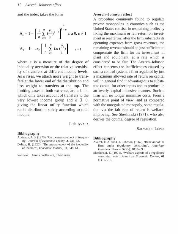
and the index takes the form

1——

l n yi l – el – e

Ae = 1 – [— ∑ (—) ] e ≥ 0, e ≠ 1n i=l m

l n yiA1 = 1 – exp[ — ∑ Ln (—)]n i=l me = 1

where e is a measure of the degree ofinequality aversion or the relative sensitiv-ity of transfers at different income levels.As e rises, we attach more weight to trans-fers at the lower end of the distribution andless weight to transfers at the top. Thelimiting cases at both extremes are e →∞,which only takes account of transfers to thevery lowest income group and e → 0,giving the linear utility function whichranks distribution solely according to totalincome.

LUÍS AYALA

BibliographyAtkinson, A.B. (1970), ‘On the measurement of inequal-

ity’, Journal of Economic Theory, 2, 244–63.Dalton, H. (1920), ‘The measurement of the inequality

of incomes’, Economic Journal, 30, 348–61.

See also: Gini’s coefficient, Theil index.

Averch–Johnson effectA procedure commonly found to regulateprivate monopolies in countries such as theUnited States consists in restraining profits byfixing the maximum or fair return on invest-ment in real terms: after the firm substracts itsoperating expenses from gross revenues, theremaining revenue should be just sufficient tocompensate the firm for its investment inplant and equipment, at a rate which isconsidered to be fair. The Averch–Johnsoneffect concerns the inefficiencies caused bysuch a control system: a firm regulated by justa maximum allowed rate of return on capitalwill in general find it advantageous to substi-tute capital for other inputs and to produce inan overly capital-intensive manner. Such afirm will no longer minimize costs. From anormative point of view, and as comparedwith the unregulated monopoly, some regula-tion via the fair rate of return is welfare-improving. See Sheshinski (1971), who alsoderives the optimal degree of regulation.

SALVADOR LÓPEZ

BibliographyAverch, H.A. and L.L. Johnson, (1962), ‘Behavior of the

firm under regulatory constraint’, AmericanEconomic Review, 52 (5), 1052–69.

Sheshinski, E. (1971), ‘Welfare aspects of a regulatoryconstraint: note’, American Economic Review, 61(1), 175–8.

12 Averch–Johnson effect

Babbage’s principleThe Englishman Charles Babbage (1791–1871) stands out in different subjects:mathematics, economics, science and tech-nology policy. Analyzing the division oflabour (1832, ch. XIX), Babbage quotesAdam Smith on the increase of productiondue to the skill acquired by repeating thesame processes, and on the causes of theadvantages resulting from the division oflabour. After saying that this divisionperhaps represents the most importanteconomic feature in a manufacturingprocess, and revising the advantages thatusually are considered a product of thisdivision, he adds his principle: ‘That themaster manufacturer, by dividing the workto be executed into different processes,each requiring different degrees of skill orof force, can purchase exactly that precisequantity of both which is necessary foreach process; whereas, if the whole workwere executed by one workman, thatperson must possess sufficient skill toperform the most difficult, and sufficientstrength to execute the most laborious, ofthe operations into which the art is divided’(pp. 175–6). Babbage acknowledges thatthe principle appeared first in 1815 inMelchiorre Gioja’s Nuovo Prospetto delleScienze Economiche.

JORDI PASCUAL

BibliographyBabbage, Charles (1832), On the Economy of Machinery

and Manufactures, London: Charles Knight; 4thenlarged edn, 1835; reprinted (1963, 1971), NewYork: Augustus M. Kelley.

Liso, Nicola de (1998), ‘Babbage, Charles’, in H.Kurzand N.Salvadori (eds), The Elgar Companion toClassical Economics, Cheltenham, UK and Lyme,USA: Edward Elgar, pp. 24–8.

Bagehot’s principleWalter Bagehot (1826–77) was an Englishhistorical economist, interested in the interre-lation between institutions and the economy,and who applied the theory of selection topolitical conflicts between nations. The prin-ciple that holds his name is about the respon-sibilities of the central bank (Bank ofEngland), particularly as lender of last resort,a function that he considered it must beprepared to develop. These ideas arose in thecourse of the debates around the passing ofthe Banking Act in 1844 and after. In an ar-ticle published in 1861, Bagehot postulatedthat the Bank had a national function, keep-ing the bullion reserve in the country. Hisopinion on the central bank statesmanshipcontrasted with the philosophy of laissez-faire, and Bagehot attempted the reconcili-ation between the service that the Bank ofEngland must render to the British economyand the profit of its stockholders.

In his Lombard Street (1873) Bagehot tookup his essential ideas published in TheEconomist, and formulated two rules in orderto check the possible panic in time of crisis: (1)the ‘loans should only be made at a very highrate of interest’; (2) ‘at this rate these advancesshould be made on all good banking securities,and as largely as the public ask for them’.

JORDI PASCUAL

BibliographyBagehot, Walter (1861), ‘The duty of the Bank of

England in times of quietude’, The Economist, 14September, p. 1009.

Bagehot, Walter (1873), Lombard Street: A Descriptionof the Money Market, reprinted (1962), Homewood,IL: Richard D. Irwin, p. 97.

Fetter, Frank Whitson (1965), Development of BritishMonetary Orthodoxy 1797–1875, Cambridge MA:Harvard University Press, pp. 169, 257–283.

13

B

Balassa–Samuelson effectThe pioneering work by Bela Balassa(1928–91) and Paul Samuelson (b.1915,Nobel Prize 1970) in 1964 provided a rigor-ous explanation for long-term deviations ofexchange rates from purchasing power parityby arguing that richer countries tend to have,on average, higher price levels than poorercountries when expressed in terms of a singlecurrency. The so-called ‘Balassa–Samuelsontheory of exchange rate determination’postulates that this long-term empirical regu-larity is due to international differences of productivity in the traded goods sector. Ina dynamic setting, since productivity gainstend to be concentrated in the traded goods sector (through faster technologicalprogress), the theory explains why fastergrowing economies tend to have higher ratesof overall price increases when expressed interms of a single currency; that is, appreciat-ing real exchange rates.

The rationale behind the explanationprovided by Balassa and Samuelson, whichleads to a dismissal of the well-knownpurchasing power parity theory as a long-term theory of exchange rate determination,runs as follows: countries tend to produceboth internationally traded and non-tradedgoods. International exchanges guaranteethat the price of traded goods is equalizedacross countries when expressed in terms ofthe same currency. However, the price ofnon-traded goods tends to be higher in thericher country, thus leading to a higher over-all price level there. Specifically, insofar asreal wages tend to move in line with labourproductivity since the richer country hashigher productivity in the manufacture oftraded goods, traded goods price equalizationleads to both real and nominal wages alsobeing higher in the traded goods sector of thericher country. As internal labour mobilityguarantees that a unique nominal wageprevails in each country, nominal wages inthe non-traded goods sector will be as high as

in the traded goods sector. Moreover, as longas international productivity differentialsacross non-traded sectors are not verypronounced, this means that the price of thenon-traded goods in the richer country willhave to be higher given the prevailing highernominal wage and the lower labour produc-tivity compared to the traded goods sector.

In a dynamic setting, the faster growingeconomy will have a relatively more rapidgrowth in the productivity of the tradedgoods sector, a correspondingly higher rateof increase in non-traded goods prices and,given the equalization of traded goods priceincreases across countries, a higher rate ofincrease in the overall price level whenexpressed in the same currency (the so-called‘Balassa–Samuelson effect’).

When examining the propositions putforward by Balassa and Samuelson, it isimportant to note, first, that it is one amongseveral competing explanations for thedriving forces behind the real exchange ratein the long term; second, it is purely asupply-side theory of relative national pricelevels with demand conditions playing norole; and third, it applies under both fixedand flexible exchange rates since it is atheory of relative prices, not absolute prices.

JOSÉ VIÑALS

BibliographyBalassa, B. (1964), ‘The purchasing power parity

doctrine: a reappraisal’, Journal of PoliticalEconomy, 72 (6), 584–96.

Canzoneri, M., R. Cumby and B. Diba (1999), ‘Relativelabor productivity and the real exchange rate in thelong run: evidence from a panel of OECD countries’,Journal of International Economics, 47, 245–66.

Samuelson, P.A. (1964), ‘Theoretical notes on tradeproblems’, Review of Economics and Statistics, 46(2), 145–54.

Banach’s contractive mapping principleStefan Banach (1892–1945) was one of themost important mathematicians of the twen-tieth century and one of the founders of

14 Balassa–Samuelson effect

modern functional analysis, several of whosefundamental notions and results, besidesBanach’s contractive mapping principle,bear his name (Banach spaces, Banach algebras, the Hahn–Banach theorem, theBanach–Steinhaus theorem, the Banach–Alaoglu theorem, the Banach–Tarski para-dox, and so on).

The most typical way of proving existenceresults in economics is by means of fixedpoint theorems. The classical Brouwer’s fixedpoint theorem for single-valued mappings andits extension to multi-valued mappings due toKakutani are widely used to prove the exis-tence of an equilibrium in several contexts.Among the many other existing fixed pointtheorems, one of the oldest, simplest butnevertheless most useful ones is Banach’sprinciple for contractive mappings from acomplete metric space into itself.

A metric space is a mathematical struc-ture consisting of a set X and a function dassigning a non-negative real number d(x,y) to each ordered pair x, y of elements in X.We can interpret the number d(x, y) as thedistance between x and y, regarded aspoints. For this interpretation to make sense,the function d should have the propertiesthat a notion of distance is expected to have:it should be symmetric, in the sense that d(x,y) = d(y, x) for any two points x and y, takethe value zero when x = y and only in thiscase, and satisfy the so-called ‘triangleinequality’: d(x, y) ≤ d(x, z) + d(z, y) for anythree points x, y and z. Then d is called adistance function and the pair (X, d) is saidto be a metric space. A metric space (X, d)is called complete when every sequence{xn} in X with the property that d(xn, xm)can be made arbitrarily small by choosing nand m sufficiently large converges to somepoint x ∈ X, which means that d(xn, x) → 0as n →∞.

Banach’s contractive mapping principlerefers to mappings T:X → X that contractdistances; that is, such that, for some positive

number a < 1 one has d(T (x), T (y)) ≤ ad (x,y) for every x, y ∈ X. Assuming that the spaceis complete, the principle establishes theexistence of a unique point x ∈ X with T (x)= x. We can say that x is the fixed point of T.

In mathematics, a typical application ofBanach’s contractive mapping principle is toprove the existence and uniqueness of solu-tions to initial value problems in differentialequations. It is used as well to establish theexistence and uniqueness of a solution toBellman’s equation in dynamic program-ming, so that it constitutes the underlyingbasic tool in the theoretical analysis of manymacroeconomic and growth models. Inmicroeconomics, it has been employed, forinstance, to prove the existence and unique-ness of Cournot equilibrium.

JUAN E. MARTÍNEZ LÓPEZ

BibliographyBanach, Stefan (1922), ‘Sur les Opérations dans les

ensembles abstraits et leur application aux équationsintégrales’, Fundamenta Mathematicae, 3, 133–81.

Van Long, Ngo and Antoine Soubeyran (2000),‘Existence and uniqueness of Cournot equilibrium: acontraction mapping approach’, Economic Letters,67 (3), 345–8.

See also: Bellman’s principle of optimality and equa-tions, Brouwer fixed point theorem, Cournot’soligopoly model, Kakutani’s fixed point theorem.

Baumol’s contestable marketsUnder partial equilibrium theory, monopolis-tic markets, if there are no economies ofscale, drive to higher prices than in the caseof effective competition. This conclusion isquestioned by the theory of contestablemarkets. William J. Baumol (b.1922) orig-inally formulated the theory in Baumol(1986) and Baumol et al. (1982). Contestablemarkets theory contends, under certainassumptions, that monopoly and efficiencyprices are not so different.

The idea is that, assuming the inexistenceof barriers to entry, a monopoly firm has no

Baumol’s contestable markets 15

other choice than to establish prices as closeas possible to efficiency or competitivemarket prices. Otherwise the monopolywould put in danger its continuity as the onlyfirm in the market. In the case where themonopolist chose to raise prices and toobtain extraordinary profits, other investorsor firms would consider entering the marketto capture all or part of the profits. Under thethreat of such a contest, the monopolistprefers to maintain prices close to costs,renouncing extraordinary benefits, but ensur-ing its permanence as a monopoly withoutcompetitors.

The consequence of the theory ofcontestable markets is that regulating byignoring control of prices and attending onlyto the raising of all the barriers to entry iseffective in achieving efficiency prices.Although the idea is quite simple, thedefence of the underlying assumptions itneeds is more difficult.

The assumptions of contestable marketsrefer, basically, to the inexistence of barriersto entry. Barriers to entry are asymmetriccosts that a new entrant has to pay whencoming into an industry or market which donot have to be currently supported by theincumbent monopoly. These costs can berelated to economic behaviour, technology,administrative procedures or legal rules. Forexample, if the monopolist behaves byreducing prices below costs temporarily toeliminate competitors (predatory behaviour),new entrants could not afford the temporarylosses and would not come into the market.In such a case, prices of the monopolist willsometimes be lower, sometimes higher, thancompetition prices. Another barrier to entryappears when consumers react not only toprices but also to other market signals. Brandand quality are product attributes differentfrom prices that have an influence onconsumers’ choice. Monopolies can beprotected by a combination of quality andbrand signals that are unaffordable to new

entrants. Again, without price regulation,prices would differ from competitive or effi-ciency prices. Generally speaking, sunk costsoperate as economic barriers to entry becausethey impose a heavy burden on the newentrants and indicate the sound commitmentof the monopoly to carry on in the industry.

Also the technology used by a monopolycould deter new entrants and constitute abarrier to entry. The existence of differenttechnologies could create asymmetries incosts and prices. Finally, administrative andlegal authorizations can also impose a different cost on new entrants vis-à-vis theincumbent monopolies. In all these cases,eliminating the control of monopoly priceswill not lead to efficiency prices.

Actually the overwhelming presence ofeconomical, technical and legal barriers toentry in industries formerly organized asmonopolies, such as power, natural gas,water or telecommunications, makes almostineffective the application of the theory ofcontestable markets to regulatory action inorder to suppress price controls.

MIGUEL A. LASHERAS

BibliographyBaumol, W.J. (1986), ‘On the theory of perfectly

contestable markets’ in J.E. Stiglitz and G.F.Mathewson (eds), New Developments in theAnalysis of Market Structure, London: Macmillan.

Baumol, W.J., J.C. Panzar and R.D. Willig (1982),Contestable Markets and the Theory of IndustryStructure, New York: Harcourt Brace Jovanovich.

Baumol’s diseaseWilliam J. Baumol (b.1922) hypothesizedthat, because labour productivity in serviceindustries grows less than in other industries,the costs in services end up rising over timeas resources move and nominal wages tendto equalize across sectors. His model ofunbalanced productivity growth predicts that(1) relative prices in sectors where produc-tivity growth is lower will rise faster; (2)relative employment will tend to rise in

16 Baumol’s disease

sectors with low productivity growth; and (3)productivity growth will tend to fall econ-omy-wide as labour moves to low-produc-tivity sectors, given a persistent demand forservices.

The evolution of developed economieshas confirmed these predictions. Prices ofpersonal services have risen, the weight ofservice employment and the size of theservice sector have increased substantially,and productivity has grown less in services.Problems are more serious in labour-inten-sive services, with little room for capitalsubstitution. It has also been argued that theyare suffered by many government activities,which would imply growing public expendi-tures. Solutions that innovate around this trapare often effective but equally often radicallyalter the nature of the service, by including init some elements of self-service and routine.Radio, records and television increased theproductivity of musical performers, but theirnew services lacked the personal characterand many other qualities of live concerts.

The root of the problem lies in a particu-lar characteristic of services, for many ofwhich consumers are the main input of theproduction process. This constrains innova-tion, because consumers often resent effortsto ‘industrialize’ production. Their com-plaints range from the depersonalization ofmedicine to being treated as objects bybureaucracies or protesting at the poor qual-ity of fast food.

BENITO ARRUÑADA

BibliographyBaumol, William J. (1967), ‘Macroeconomics of unbal-

anced growth: the anatomy of urban crisis’,American Economic Review, 57 (3), 415–26.

Baumol, William J. and Edward N. Wolff (1984), ‘Oninterindustry differences in absolute productivity’,Journal of Political Economy, 92 (6), 1017–34.

Baumol, William J., Sue Anne Batey Blackman andEdward N. Wolff (1985), ‘Unbalanced growth revis-ited: asymptotic stagnancy and new evidence’,American Economic Review, 75 (4), 806–17.

Baumol–Tobin transactions demand for cashThe interest elasticity of the demand formoney has played an important role indiscussions on the usefulness of monetarypolicy and on the comparisons betweenKeynesian, classical and monetarist views. Ifmoney is demanded as an alternative asset toother financial assets for precautionary orspeculative motives, its demand hasevidently negative interest elasticity. But itwas the merit of W.J. Baumol (b.1922) andJames Tobin (1918–2002, Nobel Prize 1981)to show in the 1950s that the transactionsdemand for cash exhibits significantly nega-tive interest elasticity. Their idea was toshow that, although the size of transactionbalances depends mainly on the volume oftransactions and on the degree of synchro-nization between individuals’ expendituresand receipts, mainly determined by institu-tional characteristics, the composition oftransaction balances is ruled by other factors.Even though there is a cost involved in theliquidation of assets, there is also an interestopportunity cost involved in the holding ofcash. Therefore individuals may wish to holdpart of their transaction balances in income-earning assets, in which case rational behav-iour leads them to maximize their netreceipts.

Baumol’s paper (1952) is an applicationof a simple model of inventory control todetermine the optimal value of each cashwithdrawal. Assume that an individual, witha value T of transactions per period, with-draws cash evenly throughout the period inlots of value C. Let b stand for the transactioncost of each withdrawal and i be the opportu-nity cost of holding cash (the interest rate).Since the individual makes T/C withdrawalsper period, his total transaction costs arebT/C. His average cash balance through theperiod is C/2, with an associated opportunitycost of iC/2. Therefore the total cost of hold-ing cash for transaction purposes is bT/C +

Baumol–Tobin transactions demand for cash 17

iC/2 and the value of C that minimizes it isthe well-known expression C = (2bT/i)1/2.Hence the interest elasticity of transactiondemand for cash equals –0.5.

In some ways Tobin’s model (1956) is anextension and generalization of Baumol’s tothe case in which transactions can take onlyintegral values. Tobin demonstrates that cashwithdrawals must be evenly distributedthroughout the period (an assumption inBaumol’s model) and discusses corner solu-tions in which, for example, optimal initialinvestment could be nil. Moreover, Tobin’smodel allows him to discuss issues related tothe transactions velocity of money and toconclude that the interest elasticity of trans-actions demand for cash depends on the rateof interest, but it is not a constant.

Finally, as in many other cases, the pri-ority of Baumol and Tobin is controversial,because Allais obtained the ‘square root’formula in 1947, as Baumol and Tobinrecognized in 1989.

JULIO SEGURA

BibliographyBaumol, W.J. (1952), ‘The transactions demand for

cash: an inventory theoretic approach’, QuarterlyJournal of Economics, 66, 545–56.

Baumol, W.J. and J. Tobin (1989), ‘The optimal cashbalance proposition: Maurice Allais’ priority’,Journal of Economic Literature, XXVII, 1160–62.

Tobin J. (1956), ‘The interest-elasticity of transactionsdemand for cash’, Review of Economics andStatistics, 38, 241–7.

See also: Hicks–Hansen model, Keynes’s demand formoney.

Bayes’s theoremThis theorem takes its name from thereverend Thomas Bayes (1702–61), a Britishpriest interested in mathematics and astron-omy. His theorem, published after his death,applies in the following situation. We havean experiment, its possible outcomes beingthe events B, C, D, E . . . For instance, we

observe the output of a production processand consider three events: the product is ofhigh quality (B), medium quality (C) or lowquality (D). The likelihood of these eventsdepends on an unknown set of causes whichwe assume are exclusive and exhaustive; thatis, one and only one of them must occur. LetAi be the event whose true cause is the ith andsuppose that we have n possible causes A1, . . ., An which have probabilities p(Ai) whereP(A1) + . . . + P(An) = 1. These probabilitiesare called prior probabilities. For instance,the process could be operating under stan-dard conditions (A1) or be out of control,requiring some adjustments (A2). We assumethat we know the probabilities p(B | Ai)which show the likelihood of the event Bgiven the true cause Ai. For instance, weknow the probabilities of obtaining asoutcome a high/medium/low-quality productunder the two possible causes: the process isoperating under standard conditions or theprocess is out of control. Then we observethe outcome and assume the event B occurs.The theorem indicates how to compute theprobabilities p(Ai | B), which are calledposterior probabilities, when the event B isobserved. They are given by

p(B | Ai)p(Ai)p(Ai | B) = ——————.

P(B)

Note that the denominator is the same for allthe causes Ai and it can be computed by

n

P(B) = ∑ p(B | Aj)p(Aj).j=1

The theorem states that the posterior prob-abilities are proportional to the product of theprior probabilities, p(Ai), and the likelihoodof the observed event given the cause, p(B |Ai).

This theorem is the main tool of the so-called ‘Bayesian inference’. In this paradigm

18 Bayes’s theorem

all the unknown quantities in an inferenceproblem are random variables with someprobability distribution and the inferenceabout the variable of interest is made byusing this theorem as follows. We have amodel which describes the generation of thedata by a density function, f (x | q), whichdepends on an unknown parameter q. Theparameter is also a random variable, becauseit is unknown, and we have a prior distribu-tion on the possible values of this parametergiven by the prior density, p(q). We observea sample from this model, X, and want toestimate the parameter that has generatedthis sample. Then, by Bayes’s theorem wehave

f (q | X) ∝ f (X | q)p(q),

which indicates that the posterior density ofthe parameter given the sample is propor-tional to the product of the likelihood of thesample and the prior density. The constant ofproportionality, required in order that f (q | X)is a density function and integrates to one, isf(X), the density of the sample, and can beobtained with this condition.

The distribution f (q | X) includes all theinformation that the sample can provide withrespect to the parameter and can be used tosolve all the usual inference problems. If wewant a point estimate we can take the modeor the expected value of this distribution. Ifwe want a confidence interval we can obtainit from this posterior distribution f (q | X) bychoosing an interval, which is called the‘credible interval’, in which the parameterwill be included with a given probability. Ifwe want to test two particular values of theparameter, q1, q2 we compare the ordinatesof both values in the posterior density of theparameter:

f(q1 | X) f (X | q1) p(q1)———— = ———— ——— .f(q2 | X) f (X | q2) p(q2)

The ratio of the likelihood of the observeddata under both parameter values is calledthe Bayes factor and this equation shows thatthe ratio of the posterior probabilities of bothhypotheses is the product of the Bayes factorand the prior ratio.

The main advantage of Bayesian infer-ence is its generality and conceptual simplic-ity, as all inference problems are solved by asimple application of the probability rules.Also it allows for the incorporation of priorinformation in the inference process. This isespecially useful in decision making, and themost often used decision theory is based onBayesian principles. The main drawback isthe need to have prior probabilities. Whenthe statistician has no prior informationand/or she/he does not want to includeher/his opinions in the inference process, aneutral or non-informative prior, sometimesalso called a ‘reference prior’, is required.Although these priors are easy to build insimple problems there is not yet a generalagreement as to how to define them incomplicated multiparameter problems.

Bayesian inference has become verypopular thanks to the recent advances incomputation using Monte Carlo methods.These methods make it feasible to obtainsamples from the posterior distribution incomplicated problems in which an exactexpression for this distribution cannot beobtained.

DANIEL PEÑA

BibliographyBayes, T. (1763), ‘An essay towards solving a problem

in the doctrine of chances’, PhilosophicalTransactions of the Royal Society, London, 53,370–418.

Bayesian–Nash equilibriumAny Nash equilibrium of the imperfect infor-mation representation, or Bayesian game, ofa normal-form game with incomplete infor-mation is a Bayesian–Nash equilibrium. In a

Bayesian–Nash equilibrium 19

game with incomplete information some orall of the players lack full information aboutthe ‘rules of the game’ or, equivalently,about its normal form. Let Gk be an N-persondecision problem with incomplete informa-tion, defined by a basic parameter space K;action sets (Ai)i∈ N and utility functions ui: K× A → R, where A = ×i∈ NAi, and it is notindexed by k ∈ K. Problem Gk does not corre-spond to any standard game-theoreticalmodel, since it does not describe the infor-mation of the players, or their strategies. k ∈K parameterizes the games that the individ-uals may play and is independent of the play-ers’ choices.

Given the parameter space K, we wouldneed to consider not only a player’s beliefsover K but also over the other players’ beliefsover K, over the other players’ beliefs overhis own beliefs and so on, which wouldgenerate an infinite hierarchy of beliefs.Harsanyi (1967–8) has shown that all this isunnecessary and Gk can be transformed into agame with imperfect information GB. In thisapproach, all the knowledge (or privateinformation) of each player i about all theindependent variables of Gk is summarizedby his type ti belonging to a finite set Ti anddetermined by the realization of a randomvariable. Nature makes the first move, choos-ing realizations t = (t1, t2, . . ., tN) of therandom variables according to a marginaldistribution P over T = T1 × . . . × TN and ti issecretly transmitted to player i. The jointprobability distribution of the tis, given byP(t), is assumed to be common knowledgeamong the players.

Then Gb = (N, (Ai)i∈ N, (Ti)i∈ N, P(t),(ui)i∈ N) denotes a finite Bayesian game withincomplete information. For any t ∈ T, P(t–i| ti) is the probability that player i wouldassign to the event that t–i = (tj)j∈ N–i is theprofile of types for the players other than i ifti were player i’s type. For any t ∈ T and anya = (aj)j∈ N ∈ A, ui(a,t) denotes the payoff thatplayer i would get if a were the profile of

actions chosen by the players and t were theprofile of their actual types.

A pure strategy of player i in Gb is amapping si: Ti → Ai, or decision rule, si(ti),that gives the player’s strategy choice foreach realization of his type ti, and player i’sexpected payoff is

ui(s1(t1), s2(t2), . . ., sN(tN)) = Et[ui(s1(t1), s2(t2), . . ., sN(tN), ti)].

Thus, a profile of decision rules (s1 (.), . . .,sN (.)) is a Bayesian–Nash equilibrium in Gb,if and only if, for all i and all t i ∈ Ti, occur-ring with positive probability

Et–i| ui(si(t i), s–i(t–i), t i | t i) |

Et–i| ui(s�i(t i), s–i(t–i), t i | t i) |

for all s�i, where the expectation is taken overrealizations of the other players’ randomvariables conditional on player i’s realizationof his signal t i.

Mertens and Zamir (1985) provided themathematical foundations of Harsanyi’stransformation: a universal beliefs spacecould be constructed that is always bigenough to serve the whole set of types foreach player. Then player i’s type can beviewed as a belief over the basic parameterand the other players’ types.

AMPARO URBANO SALVADOR

BibliographyHarsanyi, J. (1967–8), ‘Games with incomplete infor-

mation played by Bayesian players’, ManagementScience, 14, 159–82 (Part I); 320–34 (Part II);486–502 (Part III).

Mertens, J-F. and S. Zamir (1985), ‘Formulation ofBayesian analysis for games with incomplete infor-mation’, International Journal of Game Theory, 14,1–29.

Becher’s principleOne person’s expenditure is another person’sincome. Johann Joachim Becher (1635–82),in common with the majority of his European

20 Becher’s principle

contemporaries, shared a certain ‘fear ofgoods’ and, therefore, like the Englishmercantilists, he subscribed to the idea that‘it is always better to sell goods to othersthan to buy goods from others, for the formerbrings a certain advantage and the latterinevitable damage’. Within the context of hisreflections upon monetary affairs, he main-tained that people’s expenditure onconsumption is the ‘soul’ of economic life;that is, ‘one’s expenditure is another man’sincome; or that consumer expenditure gener-ates income’. He weighs up the theoreticalpossibilities of this observation, but does notdevelop a system based on this, asBoisguillebert, François Quesnay or JohnMaynard Keynes were later to do. Becher,one of the most representative cameralists,was a physician and chemist who becameadviser to Emperor Leopold I of Austria anddirector of several state-owned enterprises.He defends interventionist measures by thestate to make a country rich and populous, asthe title of his main work of 1668 indicates:Political Discourse – On the actual reasonsdetermining the growth and decline of cities,states, and republics. How to make a statepopulous and productive and to make it intoa real Civil Society.

LUIS PERDICES DE BLAS

BibliographyBecher, Johann Joachim (1668), Politischre Discurs von

den eigentlichen Ursachen dess Auff- undAbnehmens der Städt, Länder, und Republicken, inspecie, wie ein Land folckreich und nahrhafft zumachen und in eine rechte Societatem civilem zubringen; reprinted (1990) in Bibliothek Klassiker derNationalökonomie, Düsseldorf: Verlag Wirtschaftund Finanzen.

Schumpeter, Joseph A. (1954), History of EconomicAnalysis, New York: Oxford University Press.

Becker’s time allocation modelGary Becker’s (b.1930, Nobel Prize 1992)approach to consumption theory representsan important departure from conventional

theory. The distinguishing feature ofBecker’s time allocation or householdproduction model is the recognition thatconsuming market goods takes time. Thisimplies both that market goods are not directarguments of household utility functions, andthat time not spent in the labor market is notleisure any longer in Becker’s model.

The new approach introduces a new cat-egory of goods, basic goods, as the only util-ity-yielding goods. Basic goods are goodsnot purchased or sold in the market place.They are instead produced by consumers (fora given state of household technology), usingmarket purchased goods and time (non-working time) as factor inputs. Now house-holds derive utility from market goods onlyin an indirect way. Households, then, mustmake two kinds of decisions: how to produceat the minimum cost and how to consume atthe maximum utility level.

Basic goods also exhibit another charac-teristic. They have no explicit prices, sincethere are no explicit markets for them. Thisfact, however, represents no impediment tothe development of an operative theory ofhousehold behavior, as shadow prices (thatis, prices based on home production costs)can always be assigned to basic goods.Unlike market prices, shadow prices reflectthe full or effective price of goods. Fullprices depend on the price of time, the timeand market goods intensities, the price ofmarket goods and the state of householdtechnology. This brings us to a strikingconclusion. Two different consumers do notpay (in general) the same price for the samegood even if the market under considerationis perfectly competitive.

Regarding time, the crucial variable inBecker’s model, the fact that it is an input intotal fixed supply used now in both marketactivities (labor market) and non-market(home) activities has two immediate implica-tions. The first one is that ‘time is money’;that is, it has a positive price (an explicit

Becker’s time allocation model 21

price in market activities and a shadow price,approximated by the market wage rate, innon-market activities) that has to be takeninto account when analyzing householdbehavior. The second is that time not spentworking in the labor market is not leisure,but time spent in producing basic goods.These considerations together led Becker todefine a new scale variable in the utilitymaximization problem that households aresupposed to solve. It is now ‘full income’(that is, the maximum money income ahousehold can achieve when devoting all thetime and other resources to earning income)that is the relevant scale variable that limitshousehold choices.

Becker’s approach to the study of house-hold behavior implies, then, the maximiza-tion of a utility function whose arguments arethe quantities of basic goods producedthrough a well behaved production functionwhose inputs are the quantities of marketgoods and the time needed for producing thebasic goods. The household faces theconventional budget constraint and also anew time constraint which shows how fullincome is spent, partly on goods and partlyby forgoing earnings to use time in house-hold production.

A number of interesting conclusions canbe derived from the comparative statics ofBecker’s model. A central one concerns theeffects of a rise in wages. In the general caseof variable proportions technology, unlikeconventional theory, an increase in the wagerate now leads to two types of substitutioneffects. The first one is the conventionalsubstitution effect away from time spent onnon-market activities (leisure in the old fash-ioned theory). This effect leads householdsto replace time with goods in the productionof each basic good. The second type is thenew substitution effect created by thechanges in the relative full prices (or relativemarginal costs) of non-market activities thatthe increase in the wage rate induces. A rise

in the wage rate increases the relative fullprice of more time-intensive goods and thisleads to a substitution effect that moveshouseholds away from high to low time-intensive activities. This new effect changesthe optimal composition of householdproduction. The two substitution effects rein-force each other, leading to a decline in thetotal time spent consuming and an increase inthe time spent working in the labor market.

It is also of interest to note how the modelenables us to evaluate the effects fromshocks or differences in environmental vari-ables (age, education, climate and so on). Intraditional theory the effects of these vari-ables were reflected in consumers’ prefer-ences; in Becker’s theory, however, changesin these variables affect households’ produc-tion functions that cause, in turn, changes inhousehold behavior through income andsubstitution effects.

Becker’s model points out that the rele-vant measure of global production of aneconomy is far from being the one estimatedby national accounting standards. This modelhas had applications in areas such as laborsupply, the sexual division of labor, incometaxation, household technology and thecomputation of income elasticities. The newconsumption theory can explain a greatnumber of everyday facts: for example, whyrich people tend to prefer goods low in time-intensity or why women, rather than men,tend to go to the supermarket. Thanks toBecker’s work these and other ordinaryaspects of households’ behavior, attributed toexogenous factors in conventional theory(usually differences in tastes or shifts in pref-erences), can now be endogenized andrelated to differences in prices and incomes.

RAMÓN FEBRERO

BibliographyBecker, G.S. (1965). ‘A theory of the allocation of time’,

Economic Journal, 75, 493–517.

22 Becker’s time allocation model

Febrero, R. and P. Schwartz (eds) (1995), The Essenceof Becker, Stanford, California: Hoover InstitutionPress.

Bellman’s principle of optimality andequationsRichard Bellman (1920–84) received his BAfrom Brooklyn College in 1941, his MA inmathematics from the University of Wisconsinin 1943 and his PhD from PrincetonUniversity in 1946. In 1952 he joined thenewly established Rand Corporation in SantaMonica, California, where he became inter-ested in multi-stage decision processes; thisled him to the formulation of the principle ofoptimality and dynamic programming in1953.

Dynamic programming is an approachdeveloped by Richard Bellman to solvesequential or multi-stage decision problems.This approach is equally applicable for deci-sion problems where sequential property isinduced solely for computational convenience.Basically, what the dynamic programmingapproach does is to solve a multi-variableproblem by solving a series of single variableproblems.

The essence of dynamic programming isBellman’s principle of optimality. This prin-ciple, even without rigorously defining theterms, is intuitive: an optimal policy has theproperty that whatever the initial state andthe initial decisions are, the remaining deci-sions must constitute an optimal policy withregard to the state resulting from the firstdecision.

Let us consider the following optimalcontrol problem in discrete time

N–1

max J = ∑ F[x(k), u(k), k] + S[x(N)],{u(k)}N–1

k=0 k=0

subject to x(k + 1) = f[x(k), u(k), k], for k = 0,1 . . ., N – 1, with u(k) ∈ W(k), x(0) = xo.

This problem can be solved by dynamicprogramming, which proceeds backwards in

time from period N – 1 to period 0: J*N{x(N)}

= S[x(N)], and for each k ∈ {N – 1, N – 2, . . ., 1, 0},

J*{x(k)} = max {F[x(k), u(k), k] u(k)∈ W(k)

+ J*k+1{f[x(k), u(k), k]}},

which are the Bellman’s equations for thegiven problem.

EMILIO CERDÁ

BibliographyBellman, R. (1957), Dynamic Programming, Princeton,

NJ: Princeton University Press.Bellman, R. and S. Dreyfus (1962), Applied Dynamic

Programming, Princeton, NJ: Princeton UniversityPress.

Bellman, R. (1984), Eye of the Hurricane. AnAutobiography, River Edge, NJ: World ScientificPublishing Co.

Bergson’s social indifference curveLet X denote the set of all feasible economicsocial states that a society may have. Anelement x of X will be a complete descriptioneither of all goods and services that eachconsumer agent of the economy i = 1, 2, 3, . . . N may obtain or, in general, how theresources of the economy are allocated. Eachconsumer of the economy may have a utilityfunction u(i): X → R, where R stands for thereal numbers. Consider the following socialwelfare function G that assigns to each arrayof utility functions a social utility functionW: X → R; that is F = G (u(i), i = 1, 2, 3, . . .,N). The function W will represent the prefer-ences that the society may have on the socialstates. A social indifference curve will be theset of all x in X such that W(x) = c for somereal number c in R, that is, the set of allconsumption allocations with respect towhich the society will be indifferent.American economist Abram Bergson(1914–2003) was the first to propose the useof social welfare functions as a device toobtain social utility functions in order to

Bergson’s social indifference curve 23

solve the problem of how to choose amongthe different and infinite number of Paretoefficient allocations that the economy mayface. To do that, Bergson assumes that asocial welfare function is the result of certainvalue judgments that the economist mayexplicitly introduce in the analysis of theresource allocation problem. AdoptingBergson’s point of view, the economist maychoose a particular social state from thosewith respect to which the society may beindifferent.

However, Arrow (1951) shows that, ifindividual preferences, represented by util-ity functions, are ordinal and we assumethat they are non-comparable, under certainvery reasonable assumptions there is nosocial welfare function, and so no socialutility function can be used to solveBergson’s problem. Nevertheless, if theutility functions of the agents are cardinaland we allow for interpersonal comparisonsof utilities, we may have well defined socialutility functions. Examples of those func-tions are the Rawlsian social welfare func-tions W = min (u(i), i = 1, 2, 3, . . . N) andthe utilitarian social welfare function, W =∑u(i).

ANTONIO MANRESA

BibliographyArrow, K.J. (1951), Social Choice and Individual

Values, New York: John Wiley.Bergson, A. (1938), ‘A reformulation of certain aspects

of welfare economics’, Quarterly Journal ofEconomics, 52 (2), 310–34.

See also: Arrow’s impossibility theorem.

Bernoulli’s paradoxIs it reasonable to be willing to pay forparticipating in a game less than theexpected gain? Consider the followinggame, known as the St Petersburg paradox:Paul will pay to George C=1 if head appearsthe first time a coin is tossed, C=2 if the first

time that head appears is the second time thecoin is tossed, and so forth. More generally,George will receive C=2n–1 with probability(1/2)n–1 if head appears for the first time atthe nth toss. The expected gain (that is themathematical expectation) of the game is thefollowing:

1 1E(x) = — 1 + — 2 + . . .

2 4

Therefore the expected gain for George isinfinity. Paradoxically, George, or any otherreasonable person, would not pay a largefinite amount for joining Paul’s game.

One way to escape from the paradox wasadvanced by Swiss mathematician DanielBernoulli (1700–1783) in 1738, althoughCramer, in 1728, reached a similar solution.Imagine that George, instead of beingconcerned about the amount of money, ismore interested in the utility that moneyproduces for him. Suppose that the utilityobtained is the square root of the amountreceived. In that case, the expected utility ofthe game would be:

1 1 ��2E(x) = —��1 + —��2 + . . . = 1 + —— ≅ 1.71,

2 4 2

which, in terms of money, is approximatelyC=2.91. Therefore nobody as reasonable asGeorge, and with the aforementioned utilityfunction, would be prepared to pay morethan, say, C=3 for entering the game.

In fact, the solution proposed by Bernoulliwas a logarithmic utility function and,strictly speaking, it did not solve the paradox.However, his contribution is the key found-ing stone for the expected utility theory in thesense that individuals maximize expectedutility instead of expected value.

JESÚS SAURINA SALAS

24 Bernoulli’s paradox

BibliographyBernoulli, D. (1738), Specimen theoriae novae de

mesura sortis, English trans. 1954, Econometrica,22, 23–36.

See also: von Neumann-Morgenstern expected utilitytheorem.

Berry–Levinsohn–Pakes algorithm (BLP)This is an iterative routine to estimate the parameters of a model of demand andsupply for differentiated products. We have‘too many parameters’ when estimatingdemand for differentiated products. Quantitydemanded of each product is decreasing in afirm’s own price, and increasing in the priceof its rivals. A system of N goods gives N2

parameters to estimate. Berry (1994) putsome structure on the demand problem bymaking assumptions on consumer utility andthe nature of competition to reduce thenumber of parameters to estimate. Utility ofa given consumer for a given product isassumed to depend only on the interactionbetween consumer attributes and productcharacteristics, on random consumer ‘tastes’and on a small set of parameters to be esti-mated. This generalizes the multinomial logitmodel to derive demand systems with plausi-ble substitution patterns (Anderson et al.1992). Firms are assumed to be price setters.The price vector in a Nash pure-strategy inte-rior market equilibrium is a function ofmarginal costs plus mark-ups. Mark-upsdepend on price semi-elasticities, which inturn are functions of the parameters of thedemand system.

BLP algorithm estimates jointly the par-ameters of the nonlinear simultaneousdemand and pricing equations. It aggregatesby simulation, as suggested by Pakes (1986),individual consumer choices for fitting theestimated market shares and prices to thoseactually observed using the generalizedmethod of moments. The algorithm estimatesthe whole distribution of consumer prefer-ences for product characteristics from widely

available product-level choice probabilities,price data and aggregate consumer-leveldata.

JOAN-RAMON BORRELL

BibliographyAnderson, S., A. de Palma and J. Thisse (1992),

Discrete Choice Theory of Product Differentiation,Cambridge, MA: MIT Press.

Berry, S.T. (1994), ‘Estimating discrete-choice modelsof product differentiation’, RAND Journal ofEconomics, 25 (2), 242–62.

Berry, S.T., J. Levinsohn and A. Pakes (1995),‘Automobile prices in market equilibrium’,Econometrica, 63 (4), 841–90.

Pakes, A. (1986), ‘Patents as options: some estimates ofthe value of holding European patent stocks’,Econometrica, 54, 755–84.

Bertrand competition modelTwo classical assumptions are made on theinteraction among competitors in oligopolis-tic markets. If firms choose prices, they aresaid to compete ‘à la Bertrand’. If insteadthey choose quantities, they compete ‘à laCournot’. The reason for this terminology isthe work of Cournot, that deals with quanti-ties as strategic variables, and Bertrand’s(1883) sanguine review of Cournot’s bookemphasizing that firms choose prices ratherthan quantities.

As a matter of fact, the attribution toBertrand of the price competition amongoligopolists is not without controversy (seefor example, Magnan de Bornier, 1992).Cournot’s book also deals with price compe-tition, but in such a way that it is essentiallyequivalent to choosing quantities. That is, themodel proposed for price competitionassumes that each firm takes the quantityproduced by the competitors as given.Because the firm is a monopolist over theresidual demand – understood as the demandthat the firm faces once the competitors havesold – both price and quantity lead to thesame outcome.

The contribution of French mathematicianJoseph Louis François Bertrand (1822–1900)

Bertrand competition model 25

arises from the criticism of Cournot’sassumption that firms choose prices inresponse to the quantities decided bycompetitors. Instead, if the good is homoge-neous and all firms post a price that repre-sents a commitment to serve any quantity atthat price, all consumers should purchasefrom the firm with the lowest price.Therefore the residual demand curve thateach firm faces is discontinuous: it is zero ifthe firm does not have the lowest price and itcorresponds to the total demand otherwise.The results of this assumption are ratherstriking. Two firms are enough to obtain thecompetitive outcome if marginal costs areconstant and the same for both of them. Thereason is that, given any price of the competi-tors, each firm has incentives to undercut theothers in order to take all the market. Asuccessive application of this argumentmeans that the only stable price is marginalcost. Moreover, if firms have fixed costs ofproduction, the previous result also meansthat only one firm can produce in this market.

If firms differ in marginal costs, but thisdifference is not too great, the equilibriumprice corresponds to the second-lowestmarginal cost, meaning that the most effi-cient firm supplies to the whole market andmakes profits corresponding to the costdifferential. As a result, when goods arehomogeneous, profits under Bertrand com-petition are substantially lower than whenfirms compete in quantities.

Edgeworth pointed out that in the shortrun the commitment to supply unlimitedquantities is unlikely to be met. For suffi-ciently high levels of production, firms mightface increasing costs and eventually reach acapacity constraint. Under these conditions,Edgeworth also argued that a pure strategyequilibrium might fail to exist. The followingexample illustrates this point.

Consider a market with two firms, withmarginal cost equal to 0 and a productioncapacity of, at most, two units. The demand

corresponds to four consumers, with valua-tions of C=3, C=2, C=1 and C=0. In this case, bothfirms will sell up to capacity only if theycharge a price of C=0, but this price can neverbe profit-maximizing, since one of themcould raise the price to C=1 and sell one unit,with positive profits. If instead firms chargepositive prices, undercutting by one of themalways becomes the optimal strategy.

Models of horizontal differentiation orvertical differentiation, where firms vary theproduction of a good of various qualities,have extended the term ‘Bertrand competi-tion’ to differentiated products. In this case,the price–cost margin increases when theproducts become worse substitutes.

Collusion as a result of the repeated inter-action among firms has also been used torelax the results of the Bertrand model. Iffirms care enough about future profits, theymight be interested in not undercutting theirrivals if this can lead to a price war andfuture prices close to marginal cost.

In the case of both homogeneous andheterogeneous goods, the optimal price that afirm charges is increasing in the price chosenby competitors as opposed to the case ofcompetition ‘à la Cournot’, where the quan-tity produced by each firm responds nega-tively to the quantity chosen by competitors.For this reason, Bertrand competition is alsoused as an example of the so-called ‘strategiccomplements’ while quantity competition isan example of strategic substitutes.

GERARD LLOBET

BibliographyBertrand, Joseph (1883), ‘Théorie Mathématique de la

Richesse Sociale’, Journal des Savants, 67,499–508.

Magnan de Bornier, Jean (1992), ‘The Cournot–Bertrand debate: a historical perspective’, History ofPolitical Economy, 24, 623–44.

See also: Cournot’s oligopoly model, Edgewortholigopoly model, Hotelling’s model of spatialcompetition.

26 Bertrand competition model

Beveridge–Nelson decompositionIn the univariate time series analysis, thetrend component is the factor that has apermanent effect on the series. The trendmay be deterministic when it is completelypredictable, and/or stochastic when it showsan unpredictable systematic variation. Accord-ing to many economic theories, it is impor-tant to distinguish between the permanentand the irregular (transitory) movements ofthe series. If the trend is deterministic, thisdecomposition is no problem. However,when the trend is stochastic, difficulties mayarise because it may be mistaken for an irreg-ular component.

Let us consider the ARIMA (0,1,1)model:

Yt = a + Yt–1 + et + bet–1. (1)

Starting from Y0 = e0 = 0 iteration leads to

t t–1

Yt = at + (1 + b) + ∑ ei + b∑eji=1 j=1

or

t

Yt = at + (1 + b) ∑ ei – bet (2)i=1

In [2] at is the deterministic trend (DTt);

t

(1 + b)∑ eii=1

is the stochastic trend (STt); bet is the irregu-lar component (Ct). Thus Yt = DTt + STt + Ct,or Yt = DTt + Zt, Zt being the noise functionof the series.

On the other hand, DTt + STt is the perma-nent component and it is possible to provethat this component is a random walk plusdrift, so that, if the permanent component iscalled YP:

YP = a +Yt–1 + (1 + b)et

This result may be extended to any ARIMA(p,1,q).

Beveridge and Nelson (1981) show thatany ARIMA (p,1,q) may be represented as astochastic trend plus a stationary component;that is, a permanent component and an irregu-lar one.

Let us consider the noise function Z thatfollows an ARIMA (p,1,q) process, that is:

A(L) Zt = B(L) et (3)

where A(L) and B(L) are polynomials in thelag operator L of order p and q, respectivelyand et a sequence of variables of white noise.

Let us suppose that A(L) has a unit root.A(L) = (1 – L) A*(L) with A*(L) with rootsoutside the unit circle.

(1 – L) A*(L) Zt = A*(L)DZt = B(L)etDZt = A*(L)–1B(L)et= y(L)et= {y(1) + (1 – L) (1 – L)–1

[y(L) – y(1)]}et= [y(1) + (1 – L)y*(L)]et,

where y*(L) = (1 – L)–1[y(L) – y(1)]. (4)

Applying operator (1 – L) to both sides of(4), we have

t

Zt = y(1)∑ei + y*(L)et = STt + Ct,i=1

that allows the decomposition of the noisefunction into a stochastic trend component(permanent) and an irregular component(transitory).

J.B. PENA TRAPERO

BibliographyBeveridge, S. and C.R. Nelson (1981), ‘A new approach

to decomposition of economic time series intopermanent and transitory components with particular

Beveridge–Nelson decomposition 27

attention to measurement of the business cycle’,Journal of Monetary Economics, 7, 151–74.

Black–Scholes modelFischer Black (1938–1995) and MyronScholes (b.1941) asked themselves how todetermine the fair price of a financial deriva-tive as, for example, an option on commonstock. They began working together at MITin the late 1960s. Black was a mathematicalphysicist, recently graduated with a PhDdegree from Harvard, and Scholes obtainedhis doctorate in finance from the Universityof Chicago. Robert Merton, a teaching assist-ant in economics with a science degree inmathematical engineering at New York’sColumbia University, joined them in 1970.The three of them, young researchers,approached the problem using highlyadvanced mathematics. The mathematicalapproach, however, should not be surprising.In the seventeenth century, Pascal andFermat had shown how to determine the fairprice of a bet on some future event.

However, the idea of using mathematicsto price derivatives was so revolutionary thatBlack and Scholes had problems publishingtheir formula, written in a working paper in1970. Many senior researchers thought thatoptions trading was just beyond mathematicsand the paper was rejected in some journalswithout being refereed. Finally their workwas published in the Journal of PoliticalEconomy in 1973.

Merton was also very much involved inthat research and he published his own exten-sions to the formula in the same year. Notonly did the formula work, the marketchanged after its publication. Since thebeginning of trading at the Chicago BoardOptions Exchange (CBOE) in 1973, and in the first 20 years of operations, the volumeof options traded each day increased fromless than 1000 to a million dollars. Sixmonths after the original publication of theBlack–Scholes formula, Texas Instruments

designed a handheld calculator to produceBlack–Scholes option prices and hedgeratios, to be used by CBOE traders. Nowonder that the Black–Scholes formulabecame a Nobel formula. On 14 October1997, the Royal Swedish Academy ofSciences announced the winners of the 1997Nobel Prize in Economics. The winners wereRobert C. Merton and Myron S. Scholes.Fischer Black had died in 1995.

To understand the Black–Scholes formula,consider a call option of European type. Thisis a contract between a holder and a writer,which has three fixed clauses: an asset to bepurchased, a maturity date T and an exerciseprice K. The call option gives the holder theright, but not the obligation, to purchase theasset at time T for the exercise price K. TheBlack–Scholes formula computes the priceof such a contract. Conceptually, theformula is simple and it can be read as thediscounted expected benefit from acquiringthe underlying asset minus the expected costof exercising the option. To derive the math-ematical formula, some assumptions mustbe made. The key assumption is that themarket does not allow for arbitrage strate-gies, but also that the market is frictionless,the interest rate r remains constant andknown, and that the returns on the underly-ing stock are normally distributed withconstant volatility s. In the Black–Scholescontext, the fair price C for an Europeanoption at time t is computed as C = SN(d1) –Ke–r(T–t)N(d2), where S denotes the currentstock price, N is the cumulative standardnormal distribution,

ln(S/K) + (r + s2/2)(T – t)d1 =

s�����T – t

and d2 = d1 – s��t.Technically, this formula arises as the

solution to a differential equation, known inphysics as the heat equation. This equation is

28 Black–Scholes model

obtained using either an equilibrium modelwith preferences showing constant relativerisk aversion or a hedging argument, assuggested by Merton. Some general remarkscan be stated. The option price is alwayshigher than the differential between thecurrent price of the underlying and thepresent value of the exercise price. Thedifference gives the price paid for the possi-bility of a higher stock price at expiration. Onthe other hand, and this turned out to be veryimportant, the formula can be read in termsof expectations with respect to a so-called‘risk-neutral probability’ that reflects notonly the probability of a particular state ofthe world, but also the utility derived fromreceiving additional money at that state.Interestingly enough, the Black–Scholesformula calculates all these adjustmentsmathematically. Moreover, as seen from theformula, the standard deviation of the returnsis an unknown parameter. If the Black–Scholes model is correct, this parameter is aconstant and it can be implicitly derived frommarket data, being therefore a forward-looking estimate. However, it is also true thatthe underlying distribution imposed by theassumptions used by the model changes veryrapidly during the trading process. This maybe the main difficulty associated with thesuccess (or lack of success) that the formulahas these days.

EVA FERREIRA

BibliographyBlack, F. and M. Scholes (1973), ‘The pricing of options

and corporate liabilities’, Journal of PoliticalEconomy, 81 (3), 637–59.

Merton, R.C. (1973), ‘Theory of rational option pri-cing’, Bell Journal of Economics and ManagementScience, 4 (1), 141–83.

Bonferroni boundWhen constructing a confidence interval I1of an estimator b1 with Type I error a (say, 5per cent), the confidence coefficient of 1 – a

(say, 95 per cent) implies that the true valueof the parameter will be missed in a per centof the cases.

If we were to construct confidence inter-vals for m parameters simultaneously then theconfidence coefficient will only be (1 – a)m ifand only if each of the confidence intervalswas constructed from an independent sample.This is not the case when the same sample isused to test a joint hypothesis on a set of para-meters in, say, a regression model.

The Bonferroni approach, named after theItalian mathematician Emilio Bonferroni(1892–1960), establishes a useful inequalitywhich gives rise to a lower bound of the truesignificance level of the m tests performed ona given sample of observations. For illustrativepurposes, consider the case where m = 2, sothat I1 is the confidence interval of b1 withconfidence coefficient 1 – a1 whereas I2 is theconfidence interval of b2 with confidence coef-ficient 1 – a2. Then the inequality says that:

P [b1 ∈ I1 , b2 ∈ I2] ≥ 1 – a1 – a2.

This amounts to a rectangular confidenceregion for the two parameters jointly with aconfidence coefficient at least equal to 1 – a1– a2. Hence, if a1 = a2 = 0.05, the Bonferronibound implies that the rectangular confi-dence region in the b1, b2 plane has a confi-dence coefficient ≥ 0.9.

Under certain assumptions, in the test of qhypothesis in the standard linear regressionmodel with k ≥ q coefficients, the wellknown F(q, T – k) test yields ellipsoidalconfidence regions with an exact confidencecoefficient of (1 – a).

A classical reference on the constructionof simultaneous confidence intervals isTukey (1949).

JUAN J. DOLADO

BibliographyTukey, J.W. (1949), ‘Comparing individual means in the

analysis of variance’, Biometrics, 5, 99–114.

Bonferroni bound 29

Boolean algebrasThe English mathematician George Boole(1815–64) has been considered the founderof mathematical logic. He approached logicfrom an algebraic point of view and he intro-duced a new algebraic structure, calledBoolean algebra, that can be applied toseveral frameworks.

A Boolean algebra is a 6tuple �B, ∨ , ∧ , �,0, 1�, where B is a non-empty set, ∨ , ∧ twobinary operations on B (that is, x ∨ y, x ∧ y ∈B for all x, y ∈ B), � one unary operation onB (that is, x� ∈ B for all x ∈ B) and 0, 1 ∈ B,which satisfies:

1. x ∨ y = y ∨ x and x ∧ y = y ∧ x, for allx, y ∈ B (commutativity).

2. x ∨ (y ∨ z) = (x ∨ y) ∨ z and x ∧ (y ∧ z)= (x ∧ y) ∧ z, for all x, y, z ∈ B (asso-ciativity).

3. x ∨ x = x and x ∧ x = x, for all x ∈ B(idempotency).

4. x ∨ (x ∧ y) = x and x ∧ (x ∨ y) = x, forall x, y ∈ B (absortion).

5. x ∧ (y ∨ z) = (x ∧ y) ∨ (x ∧ z) and x ∨ (y∧ z) = (x ∨ y) ∧ (x ∨ z), for all x, y, z ∈B (distributivity).

6. x ∧ 0 = 0 and x ∨ 1 = 1, for all x ∈ B.7. x ∧ x� = 0 and x ∨ x� = 1, for all x ∈ B.

From the definition it follows:8. x ∧ y = 0 and x ∨ y = 1 imply x = y�, for

all x, y ∈ B.9. (x�)� = x, for all x ∈ B.

10. (x ∨ y)� = x� ∧ y� and (x ∧ y)� = x� ∨ y�,for all x, y ∈ B (De Morgan’s laws).

Typical examples of Boolean algebras are:

• B the class of all the subsets of a non-empty set X; ∨ the union, ∪ ; ∧ theintersection, ∩; � the complementation,c (that is, Ac = {x ∈ X | x ∉ A}, for allA ⊆ X); 0 the empty set, ∅ and 1 thetotal set, X.

• B the class of propositions of the clas-sical propositional logic; ∨ the disjunc-

tion; ∧ the conjuction; � the negation,¬; 0 the contradiction p ∧ ¬ p; and 1 thetautology p ∨ ¬p.

• B = {0, 1}; 0 ∨ 0 = 0, 0 ∨ 1 = 1 ∨ 0 =1 ∨ 1 = 1; 0 ∧ 0 = 0 ∧ 1 = 1 ∧ 0 = 0, 1∧ 1 = 1; 0� = 1, 1� = 0.

JOSÉ LUIS GARCÍA LAPRESTA

BibliographyBoole, G. (1847), The Mathematical Analysis of Logic.

Being an Essay Towards a Calculus of DeductiveReasoning, Cambridge: Macmillan.

Boole, G. (1854), An Investigation of the Laws ofThought, on which are Founded the MathematicalTheories of Logic and Probabilities, Cambridge:Macmillan.

Borda’s ruleThis originates in the criticism Jean-Charlesde Borda (1733–99) makes about the generalopinion according to which plural voting,that is, the election of the candidatespreferred by the greater number of voters,reflects the voters’ wishes. According toBorda, given more than two candidates (orchoices), plural voting could result in errors,inasmuch as candidates with similar posi-tions could divide the vote, allowing a thirdcandidate to receive the greatest number ofvotes and to win the election. History seemsto confirm Borda’s concern.

One example may help us to understandthis rule. Let us assume 21 voters and threecandidates X, Y and Z; seven voters opt forXZY, seven for YZX, six for ZYX and onefor XYZ. Plural voting would select X witheight votes, against Y with seven and Z withsix, who although receiving fewer votesseems a good compromise solution (thosewith a preference for X, except 1, prefer Z toY, and those with a preference for Y prefer,all of them, Z to X).

In order to solve this problem, Bordaproposed the election by ‘merit order’consisting in that each voter ranks the n-candidates in order, giving n-1 points to thepreferred one, n-2 to the second, n-3 to the

30 Boolean algebras

third, and so on (Borda’s count). Once all thepoints of each candidate are added, Borda’srule ranks the choices from highest to lowestfollowing Borda’s count. In the above exam-ple, the order would be ZYX (Z 26 points, Ywith 21 and X 16), the opposite result to theone obtained from plural voting (XYZ).

The Achilles heel of Borda’s rule is, asCondorcet had already put forward, itsvulnerability to strategic behaviour. In otherwords, electors can modify the result of thevoting, to their own advantage, by lying overtheir preference.

Borda admitted this and stated that ‘Myscheme is only intended for honest men.’ Inmodern theory of social election, startingwith Arrow’s work, Borda’s rule does notcomply with the ‘independence of irrelevantalternatives’ property, which makes thisvoting subject to manipulation.

FRANCISCO PEDRAJA CHAPARRO

BibliographyBorda, J-Ch. (1781), ‘Mémoire sur les elections au

scrutin’, Histoire de l’Académie Royale des Sciences(1784).

See also: Arrow’s impossibility theorem, Condorcet’scriterion.

Bowley’s lawIncome is distributed in a relatively constantshare between labour and capital resources.The allocation of factors reflects the maxi-mization of the company’s profits subject tothe cost function, which leads to selection oftheir relative amounts based on the relativeremuneration of the factors and on the tech-nical progress. If production were morelabour (capital)-intensive, the companywould hire more workers (capital) for a fixedwage and interest rate, which would lead toan increase in the labour (capital) share.However, what has been observed in severalcountries through the twentieth century isthat this share has been relatively constant in

the medium term, in spite of some temporaryfactors, such as taxation or the cyclical posi-tion.

Sir Arthur L. Bowley (1869–1957) regis-tered the constancy of factor shares in hisstudies for the United Kingdom in the earlytwentieth century, but many others haveaccounted later for this face in the economicliterature. No doubt technological progresshas been present in production processes,leading to an increase in the ratio of capital tolabour, but this has been counteracted by theincrease in real wages (labour productivity)in comparison with the cost of capital.Proving that the national income is propor-tionally distributed gives grounds for theacceptance of Cobb–Douglas functions torepresent production processes in a macro-economic sense.

DAVID MARTÍNEZ TURÉGANO

BibliographyBowley, A.L. (1920), ‘The change in the distribution of

the national income: 1880–1913’, in Three Studieson the National Income, Series of Reprints of ScarceTracts in Economic and Political Science, TheLondon School of Economics and Political Science(1938).

See also: Cobb–Douglas function.

Box–Cox transformationThe classical linear model (CLM) is speci-fied whenever possible in order to simplifystatistical analysis. The Box–Cox (1964)transformation was a significant contributionto finding the required transformation(s) toapproximate a model to the requirements ofthe CLM.

The most used transformation for a vari-able zt > 0; t = 1, 2, . . ., n, is

zlt – 1

; l ≠ 0zt(l) = { l

log(zt) ; l = 0, (1)

Box–Cox transformation 31

while for zt > – l2 it is

(2)

therefore the linear model relating the trans-formed variables is

k

yt(l) = b0 + ∑xi,t(li)bi + et. (3)i=1

This model is simplified when yt is the onlytransformed variable, or when there is asingle l. The Box–Cox transformation isequivalent to the family of power transfor-mations and includes (a) no transformation(l = 1), (b) logarithmic (l = 0), (c) inverse (l= –1), and (d) root square (l = 0.5).

The vector y = [l1 . . . lk; b0 . . . bk; s2],

cannot be jointly estimated by non-linearleast squares since the residual sum ofsquares may be arbitrarily made close to zerofor l → –∞ and b → 0. The usual solution is maximum likelihood, which preventsnonsensical estimates by introducing theJacobian terms, but notice that the distribu-tions of the residuals are truncated. For moregeneral transformations, see John and Draper(1980) and Yeo and Johnson (2000).

JUAN DEL HOYO

BibliographyBox, G.E.P. and D.R. Cox (1964), ‘An analysis of trans-

formations’, Journal of the Royal Statistical Society,B, 26, 211–43.

John, J.A. and N.R. Draper (1980), ‘An alternativefamily of transformations’, Applied Statistics, 29,190–97.

Yeo, In-Kwon and A. Johnson (2000), ‘A new family oftransformations to improve normality or symmetry’,Biometrika, 87, 954–9.

Box–Jenkins analysisGeorge E.P. Box (b.1919) and Gwilym M.Jenkins, in their book published in 1970,

presented a methodology for building quanti-tative models, mainly for univariate timeseries data. The term ‘Box–Jenkins method-ology’ generally refers to single time series.

The methodology proposes a class ofmodels for explaining time series data and aprocedure for building a suitable model for aspecific time series. The class of modelsproposed is called ARIMA (autoregressiveintegrated moving average) models. Whendealing with data with seasonal fluctuations,the class is restricted to ARIMA models witha multiplicative scheme.

ARIMA models are designed as relativelygeneral linear structures representing timeseries with long-run evolution (evolutionwhich tends to perpetuate itself in the future)and zero-mean stationary fluctuations aroundthem. In the absence of future shocks, thesestationary fluctuations tend towards zero. Inmany cases the long-run evolution ineconomic time series contains trend andseasonal fluctuations. In general, the trendcontains one element, level, or two elements,level and growth. In the latter case, theARIMA model for time series with noseasonal fluctuations takes the form

Xt = Xt–1 + (Xt–1 – Xt–2)

(1 – q1L – . . . – qqLq)+ at,

(1 – f1L – . . . – fpLp) (1)

where L is the lag operator and at randomshocks. The first term of the right-hand of (1)in the previous level of Xt, the second one thepast growth of Xt, and the last one its station-ary fluctuation level.

In an ARIMA model, the long-run evolu-tion results from the fact that it translates intothe future previous level and growth withunit coefficients. These coefficients refer tounit roots in the dynamic difference equationstructure that these models have.

With the ARIMA models, Box–Jenkins(1970) synthesized the results of stationary

(zt + l2)l1 – 1; l1 ≠ 0

zt(l1, l2) = { l1log(zt + l2) ; l1 = 0;

32 Box–Jenkins analysis

theory and the most useful applied timeseries procedures known at the time. Thetheory had been developed over the previous50 years by Cramer, Kinchin, Kolmogorov,Slutsky, Yule, Walker, Wold and others. Thepractical procedures had been elaborated inthe fields of exponential smoothing forecast-ing methods by, for example, Brown,Harrison, Holt, Muth and Winter, and ofseasonal adjustment at the US CensusBureau. In these two fields trend and season-ality were not considered to be deterministicbut stochastic, and it became clear in mostcases that the underlying structure wasautoregressive with unit roots.

The unit root requirement in an ARIMAmodel is based on the assumption that, bydifferentiating the data, their long-run evolu-tion is eliminated, obtaining a stationarytransformation of the original time series.Thus from (1), D2 Xt, where D = (1 – L) is thefirst difference operator, is stationary and themodel can be written in a more popular formas

(1 – f1 L – . . . – fp Lp) D2 Xt= (1 – q1 L – . . . – qq Lq) at. (2)

In this case differentiating Xt twice, weobtain stationary transformed data. A gener-alization of the example in (2), maintainingthe absence of a constant term, consists ofallowing the number of differences requiredto obtain the stationary transformation to beany integer number d. For d equals zero, theXt variable itself is stationary. For d equalsone, the trend in Xt has stochastic level but nogrowth. Usually d is no greater than two.

For the process of building an ARIMAmodel for a given time series, Box andJenkins propose an iterative strategy withthree stages: identification, estimation anddiagnostic checking. If model inadequacy isdetected in the last stage, appropriate modifi-cations would appear and with them a furtheriterative cycle would be initiated.

Extensions of the ARIMA model allow-ing the parameter d to be a real number havebeen proposed with the fractionally inte-grated long-memory process. This process(see Granger, 2001) has an ‘interestingtheory but no useful practical examples ineconomics’.

Zellner and Palm (1974) and, later, otherauthors such as Wallis, connected theARIMA models with econometric models byshowing that, under certain assumptions, theARIMA model is the final form derived foreach endogenous variable in a dynamicsimultaneous equation model. Therefore theuse of an ARIMA model for a certain vari-able Xt is compatible with the fact that Xt isexplained in a wider econometric model.

This connection shows the weakness andpotential usefulness of ARIMA models ineconomics. The limitations come mainlyfrom the fact that univariate models do notconsider relationships between variables.Thus Granger (2001) says, ‘univariate modelsare not thought of as relevant models for mostimportant practical purposes in economics,although they are still much used as experi-mental vehicles to study new models andtechniques’. ARIMA models in themselvesturned out to be very successful in forecastingand in seasonal adjustment methods. Thesuccess in forecasting is (see Clements andHendry, 1999) especially due to the presenceof unit roots. In practice, agents want not onlyreliable forecasts, but also an explanation ofthe economic factors which support them. Bytheir nature, ARIMA models are unable toprovide this explanation. It requires thecongruent econometric models advocated inClements and Hendry, updating them eachtime a structural break appears. For the timebeing, the building of these models forgeneral practice in periodical forecastingcould in many cases be complex and costly.

ANTONI ESPASA

Box–Jenkins analysis 33

BibliographyBox, G.E.P. and G.M. Jenkins (1970), Time Series

Analysis, Forecasting and Control, San Francisco:Holden-Day.

Granger, C.W.J. (2001), ‘Macroeconometrics – past andfuture’, Journal of Econometrics, 100, 17–19.

Clements, M.P. and D. Hendry (1999), ForecastingNon-stationary Economic Time Series, London:MIT Press.

Zellner, A. and F. Palm (1974), ‘Time series analysisand simultaneous equation econometric models’,Journal of Econometrics, 2 (1), 17–54.

Brouwer fixed point theoremLuitzen Egbertus Jan Brouwer (1881–1966)was a Dutch mathematician whose mostimportant results are characterizations oftopological mappings of the Cartesian planeand several fixed point theorems.

This theorem states: let f : X → X be acontinuous function from a non-empty,compact and convex set X ⊂ Rn into itself.Then f has a fixed point, that is, there existsx� ∈ X such that x� = f (x�).

This theorem is used in many economicframeworks for proving existence theorems.We mention some of the most relevant. Johnvon Neumann, in 1928, proved the minimaxtheorem. He established the existence of apair of equilibrium strategies for zero-sumtwo-person games; that is, the existence of asaddle-point for the utility of either player.Existence of general equilibrium for acompetitive economy was proved by Arrowand Debreu in 1954. Herbert Scarf used it inthe computation of economic equilibrium.Hirofumi Uzawa proved, in 1962, the exist-ence of Walrasian equilibrium.

GUSTAVO BERGANTIÑOS

BibliographyBrouwer, L.E.J. (1912), ‘Uber Abbildung von

Mannigfaltikeiten’, Mathematische Annalen, 71,97–115.

See also: Arrow–Debreu general equilibrium model;Kakutani’s fixed point theorem.

Buchanan’s clubs theoryThe theory of clubs is part of the theory ofimpure public goods. When James M.Buchanan (b.1919, Nobel Prize 1986) wrotehis seminal piece (1965), the theory ofpublic goods was barely developed, and hewas able to fill the Samuelsonian gapbetween private and pure public goods.Buchanan demonstrated how the conditionsof public good provision and club member-ship interact.

A club good is a particular case of publicgood, which has the characteristics ofexcludability and non-rivalry (or partial non-rivalry, depending on the congestion). Bycontrast, a pure public good has the charac-teristic of both non-excludability and non-rivalry.

Therefore a club is a voluntary group ofindividuals deriving mutual benefit fromsharing either the cost of production or themembers’ characteristics or an impure publicgood. A club good is characterized byexcludable benefits. The fundamental char-acteristic of the club is its voluntary member-ship. Its members take the decision to belongto the club because they anticipate the bene-fits of the collective provision from member-ship.

For this reason, a club good is excludableand this is its main characteristic, because,without exclusion, there would be no incen-tives to belong to the club and pay fees orrights to enter. Therefore, in contrast to purepublic goods, it is possible to prevent itsconsumption by the people that will not payfor it. However the club good keeps thecharacteristic of non-rivalry; that is, theconsumption of the good by one person doesnot reduce the consumption of the samegood by others, except when congestionhappens and the utility of any individual willbe affected by the presence of moremembers of the club. Rivalry and congestionincrease when the number of individualssharing the same club good increases too.

34 Brouwer fixed point theorem

Buchanan’s analysis includes the club-sizevariable for each and every good, whichmeasures the number of persons who are tojoin in the consumption arrangements for theclub good over the relevant time period. Theswimming pool is the original example of aclub good in Buchanan’s article. The usersthat share a swimming pool suffer rivalry andcongestion when the number of membersincreases.

Another pioneering club model is that ofCharles Tiebout (1956) whose ‘voting withthe feet’ hypothesis attempted to show howthe jurisdictional size of local governmentscould be determined by voluntary mobilitydecisions. In this model, the amount of theshared local public good is fixed and distinctfor each governmental jurisdiction and thedecentralized decision mechanism allowsachieving Pareto optimality for local publicgoods. Most of the articles analysing thetheory of club goods have been written sinceBuchanan’s seminal article; however theroots go back to the 1920s, to A.C. Pigou andFrank Knight, who applied it to the case oftolls for congested roads.

JORDI BACARIA

BibliographyBuchanan, J.M. (1965), ‘An economic theory of clubs’,

Economica, 32, 1–14.Tiebout, C.M. (1956), ‘A pure theory of local expendi-

tures’, Journal of Political Economy, 64, 416–24.

See also: Tiebout’s voting with the feet process.

Buridan’s assOften mentioned in discussions concerningfree will and determinism, this refers to anass placed equidistant from two equalbundles of hay; lacking free will, it cannotchoose one or the other and consequentlystarves to death. The paradox is named afterthe French medieval philosopher JeanBuridan (1300–58), who studied at theUniversity of Paris under nominalist Williamof Occam, and was later professor and rectorof the university. He supported the scholasticscepticism that denied the distinctionbetween the faculties of the soul: will andintellect being the same, man, who has freewill, must choose the greatest good, andcannot do it facing two equally desirablealternatives. The theory was ridiculed by hiscritics with the tale of Buridan’s ass, notpresent in his writings; they stated that thehuman being has free will, a faculty of themind that is able to create a preference with-out sufficient reason. Sen (1997) illustratesthe fundamental contrast between maximiz-ing and optimizing behaviour with Buridan’sass and, according to Kahabil (1997) thestory suggests that mere logical deduction isinsufficient for making any decision, and thatrisk taking is safer than security seeking.

VICTORIANO MARTÍN MARTÍN

BibliographyKahabil, Elias L. (1997), ‘Buridan’s ass, uncertainty,

risk and self-competition: a theory of entrepreneur-ship’, Kyklos, 2 (50), 147–64.

Sen, A. (1997), ‘Maximization and the act of choice’,Econometrica, 4 (65), 745–9.

Buridan’s ass 35

Cagan’s hyperinflation modelNamed after the American economist PhillipD. Cagan (b.1927), this is a monetary modelof hyperinflation that rests on three buildingblocks: first, there is a demand for realmoney balances that depends only onexpected inflation; second, expected infla-tion is assumed to be determined by an adap-tive rule where the expected inflation isrevised in each period in proportion to theforecast error made when predicting the rateof inflation in the previous period; third, themoney market is always in equilibrium.

The main objective in Cagan’s (1956)pioneering paper was identifying a stabledemand for money during hyperinflationaryepisodes. He observed that these are charac-terized by huge rates of inflation (forinstance, monthly rates of inflation higherthan 50 per cent) and a sharp fall in realmoney balances. Cagan postulated that thedemand for real money balances is only afunction of the expected rate of inflationduring hyperinflation; that is, real moneybalances are inversely related to the expectedopportunity cost of holding money instead ofother assets. His intuition was that, duringhyperinflationary periods, the variation in thereal variables determining the demand forreal money balances during regular periods(for instance, real income and real interestrate) is negligible compared to the variationof relevant nominal variables. The demandfor money can then be isolated from any realvariable and can be expressed only in termsof nominal variables during hyperinflation:in particular, in terms of the anticipated rateof inflation.

Specifically, Cagan’s money demandpostulates that the elasticity of the demandfor real money balances is proportional to the

expected rate of inflation. An implication ofthis is that changes in the expected rate ofinflation have the same effect on real moneybalances in percentage terms, regardless ofthe level of real money balances. Thereforethis feature postulates a notion of stability forthe demand for real money balances in ascenario characterized by a bizarre behaviorof nominal variables. Cagan studied sevenhyperinflationary episodes that developed insome central European countries in the 1920sand 1940s. He provided evidence that hissimple money demand model fits well withthe data from those hyperinflations. Sincethen, a great number of papers have shownthat Cagan’s model is a useful approach tounderstanding hyperinflationary dynamics.More importantly, perhaps, Cagan’s model isconsidered one of the simplest dynamicmodels used in macroeconomics to studyrelevant issues. Among other issues, Cagan’smodel has been used, as a basic framework,to analyze the interaction between monetaryand fiscal policies, expectations formation(rational expectations and bounded ration-ality), multiplicity of equilibria, bubbles andeconometric policy evaluation.

JESÚS VÁZQUEZ

BibliographyCagan, P.D. (1956), ‘Monetary dynamics of hyperinfla-

tion’, in Milton Friedman (ed.), Studies in theQuantity Theory of Money, Chicago: University ofChicago Press.

See also: Baumol–Tobin transactions demand forcash, Keynes’s demand for money, Muth’s rationalexpectations.

Cairnes–Haberler modelNamed after John E. Cairnes (1823–75) andG. Haberler (1901–95), this model is used for

36

C

analyzing the gains from international tradein terms of comparative advantage in thevery short run. It is formulated as a two coun-tries–two goods–three factors model, on thebasis that, in the very short run, it seemsreasonable to assume that virtually all factorsof production are immobile between sectors.This means that production proportions arefixed, so marginal physical products areconstant. As a consequence, if commodityprices are fixed, factor payments will befixed too. In this context, changes incommodity prices will imply that returns toall factors in an industry change by the sameproportion that the price changes.

YANNA G. FRANCO

BibliographyKrugman, Paul R. and Maurice Obstfeld (2003),

International Economics, 6th edn, Boston: AddisonWesley, Chapter 2.

Cantillon effectThe Cantillon effect is the temporary andshort-run effect on the structure of relativeprices when a flow of liquidity (usuallyspecie) gets into the market. Such an effect isrelated to the monetary theory of RichardCantillon (1680?–1734) and the use of thequantity of money to explain the price level.In his exposition of the quantity theory,Cantillon distinguished between differentways in which a flow of money (specie)enters the economy. Undoubtedly, themoney inflow will finally have as a result anincrease in prices, taking into account thevolume of output and the velocity of circula-tion, but until the mechanism acts upon theprice level, the money passes through differ-ent hands and sectors, depending on the wayit has been introduced. In Cantillon’s words,Locke ‘has clearly seen that the abundance ofmoney makes every thing dear, but he hasnot considered how it does so. The greatdifficulty of this question consists in know-

ing in what way and in what proportion theincrease of money rises prices’ (Cantillon[1755] 1931, p. 161).

So, although an increase of actual moneycauses a corresponding increase of consump-tion which finally brings about increasedprices, the process works gradually and, in theshort run, money will have different effects onprices if it comes from mining for new goldand silver, if it proceeds from a favourablebalance of trade or if it comes from subsidies,transfers (including diplomatic expenses),tourism or international capital movements. Inevery case, the prices of some products willrise first, and then other prices join the risingprocess until the increase gradually spreadsover all the economy; in each case marketsand prices affected in the first place are differ-ent. When the general price level goes up,relative prices have been altered previouslyand this means that all economic decisionsand equilibria have changed, so ‘Marketprices will rise more for certain things than forothers however abundant the money may be’(ibid., p. 179). This is the reason why anincreased money supply does not raise allprices in the same proportion.

Cantillon applied this effect to his analy-sis of the interest rate. Although he presentswhat we may consider a real theory of inter-est, he accepts that an injection of currencybrings down the level of interest, ‘becausewhen Money is plentiful it is more easy tofind some to borrow’. However, ‘This idea isnot always true or accurate.’ In fact, ‘If theabundance of money in the State comes fromthe hands of money-lenders it will doubtlessbring down the current rate of interest . . . butif it comes from the intervention of spendersit will have just the opposite effect and willraise the rate of interest’(ibid., pp. 213, 215).This is an early refutation of the idea thatclassical economists believed in the neutral-ity of money.

FERNANDO MÉNDEZ-IBISATE

Cantillon effect 37

BibliographyCantillon, Richard (1755), Essai sur la Nature du

Commerce en Général, English translation and othermaterials by H. Higgs (ed.) (1931), London:Macmillan.

Cantor’s nested intervals theoremGeorg Cantor (1845–1918) was a Germanmathematician (although he was born in St.Petersburg, Russia) who put forward themodern theory on infinite sets by building ahierarchy according to their cardinal number.He strongly contributed to the foundations ofmathematics and, in fact, his achievementsrevolutionized almost every field of math-ematics. Here we shall offer two importantresults of Cantor that are widely used in bothpure mathematics and applications.

Nested intervals theoremLet [an, bn]n∈ N be a decreasing sequence ofintervals of R, (that is, [an+1, bn+1] ⊆ [an,bn]), such that limn→∞ [bn – an] = 0. Thenthere is a single point that belongs to everyinterval [an, bn].

This theorem can be generalized to higherdimensions or even to more abstract spaces.In particular, its version for metric spaces isof great relevance. It states that the intersec-tion of a decreasing sequence of non-empty,closed subsets of a complete metric spacesuch that the diameter (roughly speaking, thegreatest of the distance among two arbitrarypoints of the set) of the sets converges to zeroconsists exactly of one point.

Order type of the rationalsAny numerable totally ordered set that isdense and unbordered is isomorphic to theset of rational numbers, endowed with itsnatural order.

In simple words, this result says that thereis only one numerable totally ordered set thathas no gaps and no limits, namely, the set ofthe rationals. This theorem has a notablesignificance in the mathematical foundationsof decision analysis. In particular, it is used

to construct utility functions on certain topo-logical spaces.

JAN CARLOS CANDEAL

BibliographyBell, E.T (1986), Men of Mathematics: The Lives and

Achievements of Great Mathematicians from Zeno toPoincaré, New York: Simon and Schuster.

Bridges, D.S. and G.B. Mehta, (1995), Representationsof Preference Orderings, Lecture Notes inEconomics and Mathematical Systems, Berlin:Springer-Verlag.

Rudin, W. (1976), Principles of Mathematical Analysis,3rd edn, New York: McGraw-Hill.

See also: Cauchy’s sequence.

Cass–Koopmans criterionThis is also termed the Ramsey–Cass–Koopmans condition of stationary equilib-rium in an economy characterized by arepresentative consumer that maximizesintertemporal discounted utility subject to a budget constraint and a production con-straint. It basically says that, in order tomaximize their utility, consumers mustincrease consumption at a rate equal to thedifference between, on the one hand, therate of return on capital and, on the otherhand, the discount rate plus the rate atwhich technology grows, and save accord-ingly. At steady-state equilibrium, however,this difference is nil, so that consumptionand saving per worker remain constant.Strictly speaking, the Cass–Koopmanscriterion refers to the steady-state con-dition in an economy with endogenoussaving.

Formally stated, the above conditions are

dct/dt 1—— = — (f �(kt) – r – qg),

ct q

for optimal consumption and saving andf ′(k*) = r + qg for the steady state where c isconsumption, 1/q is the elasticity of substitu-tion, k is capital per worker, r is the time

38 Cantor’s nested intervals theorem

discount rate and g is the growth rate of tech-nology.

David Cass (b.1937) and TjallingKoopmans (1910–86) developed theirmodels in the early 1960s by addingconsumption and savings behaviour to theSolow model developed some years before.The way to do it was already established byFrank Ramsey in his seminal EconomicJournal paper of 1928. The Cass–Koopmanscriterion, incidentally, is related to theHotelling rule for optimal depletion of anexhaustible resource, as the time discountrate plays a similar role in both.

JOSÉ A. HERCE

BibliographyCass D. (1965), ‘Optimum growth in an aggregative

model of capital accumulation’, Review of EconomicStudies, 32, 233–40.

Koopmans T.C. (1965), ‘On the concept of optimalgrowth’, Cowles Foundation Paper 238, reprintedfrom Academiae Scientiarum Scripta Varia, 28 (1).

Ramsey F.P. (1928), ‘A mathematical theory of saving’,Economic Journal, 38, 543–59.

See also: Radner’s turnpike property, Ramsey modeland rule, Solow’s growth model and residual.

Cauchy distributionThe Cauchy distribution (Augustin–LouisCauchy, 1789–1857) has probability densityfunction

x – q 2 –1

f(x) = (pl)–1[1 + ( ——) ]l,

where q is the location parameter and l thescale parameter. This distribution is bestknown when q = 0, l = 1; the density thenreduces to 1/p(1 + x2) and is called a ‘stan-dard Cauchy’. Its shape is similar to that of astandard normal, but it has longer and fattertails. For this reason it is often used to studythe sensitivity of hypothesis tests whichassume normality to heavy-tailed departuresfrom normality. In fact, the standard Cauchy

is the same as the t distribution with 1 degreeof freedom, or the ratio of two independentstandard normals.

The Cauchy distribution is probably bestknown as an example of a pathological case.In spite of its similarity to the normal distri-bution, the integrals of the form ∫xr ƒ(x)dx donot converge in absolute value and thus thedistribution does not have any finitemoments. Because of this, central limit the-orems and consistency results for ordinaryleast squares estimators do not apply. A moreintuitive expression of this pathologicalbehaviour is that the sample mean from arandom sample of Cauchy variables hasexactly the same distribution as each of thesample units, so increasing the sample sizedoes not help us obtain a better estimate ofthe location parameter.

The distribution became associated withCauchy after he referred to the breakdown ofthe large sample justification for leastsquares in 1853. However, it seems that thisand other properties of the standard Cauchydensity had been known before.

PEDRO MIRA

BibliographyCauchy, A.L. (1853), ‘Sur les résultats moyens d’obser-

vations de même nature, et sur les résultats les plusprobables’, Comptes Rendus de l’Académie desSciences, Paris, 37, 198–206.

Johnson, N.L., S. Kotz and N. Balakrishnan (1994),‘Cauchy distribution’, Continuous UnivariateDistributions, vol. 1, New York: John Wiley, ch. 16.

NIST/SEMATECH e-Handbook of Statistical Methods(2003), ‘Cauchy distribution’, http://www.itl.nist.gov/div898/handbook/.

Cauchy’s sequenceAugustin-Louis Cauchy (1789–1857) was aFrench mathematician whose contributionsinclude the study of convergence and divergence of sequences and infinite series,differential equations, determinants, proba-bility and mathematical physics. He alsofounded complex analysis by discovering the

Cauchy’s sequence 39

Cauchy–Riemann equations and establishingthe so-called ‘Cauchy’s integral formula’ forholomorphic functions.

A sequence (an)n∈ N is called a ‘Cauchysequence’ (or is said to satisfy the Cauchycondition) if, for every ∈ > 0, there exists p∈ N such that, for all m, n ≥ p, | xn – xm | < ∈ .

It can be proved that, for a real sequence,the Cauchy condition amounts to the conver-gence of the sequence. This is interestingsince the condition of being a Cauchysequence can often be verified without anyknowledge as to the value of the limit of thesequence.

Both the notions of a Cauchy sequenceand the Cauchy criterion also hold in higher(finite or infinite) dimensional spaces wherethe absolute value function | . | is replacedby the norm function || . ||. Furthermore, aCauchy sequence can be defined on arbi-trary metric spaces where the distance func-tion plays the role of the absolute valuefunction in the above definition. It is easilyseen that every convergent sequence of ametric space is a Cauchy sequence. Themetric spaces for which the converse alsoholds are called complete. Put into words, ametric space is complete if every Cauchysequence has a limit. Examples of completemetric spaces include the Euclidean spacesRn, n ≥ 1, or much more sophisticated oneslike C [0, 1] the Banach space that consistsof the continuous real-valued functionsdefined on [0, 1], endowed with the supre-mum distance. The notion of Cauchysequence can also be generalized foruniform topological spaces.

JAN CARLOS CANDEAL

BibliographyBell, E.T. (1986), Men of Mathematics: The Lives and

Achievements of Great Mathematicians from Zeno toPoincaré, New York: Simon and Schuster.

Berberian, S.K. (1994), A First Course in Real Analysis,Berlin: Springer-Verlag.

Rudin, W. (1976), Principles of Mathematical Analysis,3rd edn, New York: McGraw-Hill.

See also: Banach’s contractive mapping principle,Euclidean spaces.

Cauchy–Schwarz inequalityThis inequality bears the names of two of thegreatest mathematical analysts of the nine-teenth century: Augustin–Louis Cauchy, aFrenchman, and Hermann Amandus Schwarz,a German. A ubiquitous, basic and simpleinequality, it is attributed also to ViktorYakovlevich Bunyakovski, a Russian doctoralstudent of Cauchy. There are so many namesbecause of different levels of generality, andcertain issues of priority.

In its simplest form, the inequality statesthat, if (ai)

ni=1 and (bi)

ni=1 are lists of real

numbers, then:

n 2 n n(∑aibi) ≤ (∑ai2)(∑bi

2).i i i

It is most easily derived by expanding bothsides and by using the inequality 2xy ≤ (x2 +y2) (which is another way of writing theobvious (x – y)2 ≥ 0) with x = aibj and y =ajbi. This is actually the argument thatappears in Cauchy (1821) in the notes to thevolume on algebraic analysis.

The inequality may be viewed as a resultabout vectors and inner products, because ifv→ = (a1, a2, . . ., an) and w→ = (b1, b2, . . ., bn)then it translates into

| v→ · w→ | ≤ || v→ || || w→ ||

Observe that, geometrically, the inequal-ity means that | cos q | ≤ 1, where q is theangle between the two vectors. But its realinterest rests in that it holds not only forvectors in Euclidean space but for vectors inany vector space where you have defined aninner product and, of those, you haveplenty.

For example, we could consider continu-ous functions f, g in the interval [0, 1] anddeduce that

40 Cauchy–Schwarz inequality

(∫1

0f (x)g(x)dx) ≤ (∫

1

0f (x)2dx)1/2 (∫

1

0g(x)2dx)1/2,

which is an instance of the more generalHölder’s inequality,

(∫1

0f (x)g(x)dx) ≤ (∫

1

0f (x)pdx)1/p (∫

1

0g(x)qdx)1/q,

whenever p, q > 0 verify

1 1— + — = 1.p q

Or we could consider random variables Xand Y (with finite second moments), anddeduce the fundamental fact cov (X, Y ) ≤ var(X)1/2 var (Y )1/2. The general vector inequal-ity follows by observing that the parabola y =|| v→ – xw→ || attains its (positive) minimum at x= (v→ · w→)/|| w→ ||2.

What about equality? It can only takeplace when the two vectors in question areparallel, that is, one is a multiple of the other.Observe that the covariance inequality abovesimply says that the absolute value of thecorrelation coefficient is 1 only if one of therandom variables is a linear function of theother (but, at most, for a set of zero probabil-ity).

Let us consider one particular case of theoriginal inequality: each bi = 1, so that wemay write it as:

∑niai ∑n

ia2i| —— | ≤ | ——— |1/2

n n

and equality may only occur when the ais areall equal. So the quotient

∑nia

2i ∑n

iai| ——— | / | ——— |2

n n

is always at least one and measures howclose the sequence (ai)

ni=1 is to being

constant. When ai = (xi – x —)2, this quotient

measures the kurtosis of a sample (xi)ni=1 with

mean x — (one usually subtracts 3 from thequotient to get the kurtosis).

Suppose, finally, that you have n compa-nies competing in a single market and thatcompany i, say, controls a fraction ai of thatmarket. Thus ∑n

i=1ai = 1, and the quotient

∑nia

2i ∑n

iai| ——— | / | ——— |2

n n

which, in this case, is equal to

n(∑ai2) n

i

measures how concentrated this market is: avalue close to one means almost perfectcompetition, a value close to n means heavyconcentration. This quotient is essentially theHerfindahl index that the Department ofJustice of the United States uses in antitrustsuits.

JOSÉ L. FERNÁNDEZ

BibliographyCauchy, Augustin-Louis (1821), Cours d’Analyse de

L’Ecole Polytechnique, Paris.

See also: Herfindahl-Hirschman index.

Chamberlin’s oligopoly modelThe model proposed by Edward Chamberlin(1899–1967) in 1933 analyses a marketstructure where there is product differentia-tion. Specifically, he defines a market with ahigh number of firms, each selling similarbut not identical products. Consumersconsider those products as imperfect substi-tutes and therefore their demand curves havesignificant cross-price elasticities. Eachproducer is a monopolist of his productfacing a demand curve with negative slope.However, he competes in the market with theother varieties produced by the rest of the

Chamberlin’s oligopoly model 41

firms. Chamberlin also assumes free entryand consequently in the long-run equilibriumthe profit of all firms is nil. For these charac-teristics, the market structure defined byChamberlin is also known as ‘monopolisticcompetition’. This model has been used inmany theoretical and empirical papers oninternational trade.

In the short run, the number of firms andtherefore the number of products is fixed.The monopolistic competition equilibrium isvery similar to the monopoly equilibrium inthe sense that each producer is a price makerof his variety. However, in the context ofmonopolistic competition, the price that theconsumer is willing to pay for the product ofeach firm depends on the level of productionof the other firms. Specifically, the inversedemand function of firm i can be expressedas pi = pi(xi, x–i) where

N

x–i = ∑xj.j=1j≠1

In the Chamberlin analysis, each firmassumes a constant behavior of the otherfirms. That is, each producer assumes that allthe producers of other commodities willmaintain their prices when he modifies his.However, when competitors react to his pricepolicy, the true demand curve is differentfrom the demand curve facing each firm. Inequilibrium, the marginal revenue of bothdemand curves should be the same for thelevel of production that maximizes profit.Therefore each firm’s forecasts must becompatible with what the other firms actuallydo. In the equilibrium of monopolisticcompetition in the short run, (x*

1, . . ., x*N), it

must be satisfied that MRi(x*i, x

*–i) = MCi(x

*i,

x*–i) i = 1 . . . N. For each firm, its marginal

revenue equals its marginal cost, given theactions of all producers.

When the firms obtain positive profits inthe short run, new firms will enter the indus-

try, reducing the demand curve of the incum-bents. In the long-run equilibrium, the profitsof all firms will be zero and therefore theprice must equal average cost. As thedemand curve facing each has negativeslope, the equilibrium is obtained for a levelof production which is lower than the mini-mum average cost that will be the equilib-rium without product differentiation (theperfect competition). This result implies thatthe monopolistic competition equilibriumexhibits excess capacity. However, if theproducts are close substitutes and the firmscompete in prices, the demand curve will bevery elastic and the excess capacity will besmall. On the other hand, although the equi-librium will be inefficient in terms of costbecause price exceeds marginal cost, it canbe socially beneficial if consumers like prod-uct diversity.

LOURDES MORENO MARTÍN

BibliographyChamberlin, E.H. (1933), The Theory of Monopolistic

Competition (A Re-orientation of the Theory ofValue), Oxford University Press.

Dixit, A. and J.E. Stiglitz (1977), ‘Monopolistic compe-tition and optimum product diversity’, AmericanEconomic Review, 67, 297–308.

Spence, M. (1976), ‘Product selection, fixed cost andmonopolistic competition’, Review of EconomicStudies, 43, 217–35.

See also: Dixit–Stiglitz monopolistic competitionmodel.

Chipman–Moore–Samuelson compensation criterionThis criterion (hereafter CMS) tries to over-come the relative ease with which incon-sistent applications of the Kaldor–Hicks–Scitovski criterion (hereafter KHS) can beobtained. According to this criterion, alterna-tive x is at least as good as alternative y if anyalternative potentially feasible from y isPareto-dominated by some alternative poten-tially feasible from x. It has the advantage of

42 Chipman–Moore–Samuelson compensation criterion

providing a transitive (although typicallyincomplete) ranking of sets of alternatives.

The problem with the CMS criterion,contrary to the KHS criterion, is that it doesnot satisfy the Pareto principle. The CMScriterion is concerned only with potentialwelfare and it says nothing about actualwelfare as evaluated by the Pareto principle.

The non-crossing of utility possibilityfrontiers is necessary and sufficient for thetransitivity of the KHS criterion and for theCMS criterion to be applied in accordancewith the Pareto principle without inconsist-encias.

LUÍS A. PUCH

BibliographyGravel, N. (2001), ‘On the difficulty of combining

actual and potential criteria for an increase in socialwelfare’, Economic Theory, 17 (1), 163–80.

See also: Hicks’s compensation criterion, Kaldorcompensation criterion, Scitovsky’s compensationcriterion.

Chow’s testIntroduced in 1960 by Gregory Chow(b.1929) to analyse the stability of coeffi-cients in a model and it is based on thecomparison of residual sum of squares (RSS),between two periods by means of an F statis-tic which should have values lower than Fawhen the hypothesis of homogeneity of para-meters is true. There are two types of Chow’stest: one for within-sample comparison, withestimation of a common sample and twoseparate subsamples; another for post-samplecomparison, with a common estimation forsample and post-sample periods and anotherestimation for the sample period.

The first type consists of estimating threerelations, one for all the sample period andone for each of the two subsamples, andcompares the value of the statistic F =(DRSS/dfn)/((RSS1 + RSS2)/dfd) with thecorresponding significant value Fa, being

DRSS = RSS – (RSS1 + RSS2), the increase inRSS between the joint sample and the twosubsamples, and being dfn/dfd, the degrees offreedom of numerator/denominator, as to saydfn = (T – k – 1) – (T1 – k – 1) – (T2 – k – 1)= k, and dfd = (T1 – k – 1) + (T2 – k – 1) = T– 2 (k + 1), where k + 1 is the number of para-meters in the model, and T = T1 + T2 is thesample size.

The second type consists of the compari-son of the value of the statistic F = [(RSS –RSS1)/n]/[RSS1/(T – k – 1)], based on the esti-mation of the common sample of size T + nand a first sample of size T, n being the sizeof the forecasting period. This second typecan also be used for within-sample compari-son when the breaking point leaves a verysmall sample size for the second subsample.The test assumes the existence of homogen-eity in the variance of the random shock.This author has had an important influenceon the application of both types of test,which have been highly useful for many rele-vant econometric applications. Generally thelack of stability is due to the omission of oneor more relevant variables and the test is ofgreat help to show that problem in order toimprove the model specification.

M. CÁRMEN GUISÁN

BibliographyChow, G.C. (1960), ‘Tests of equality between sets of

coefficients in two linear regressions’, Econo-metrica, 28, 591–605.

Clark problemThis refers to J.B. Clark’s fast and deep shiftfrom social historicism to neoclassicaleconomics. John Bates Clark (1847–1938)graduated from Amherst College, Massa-chusetts, in 1875 and then went to Heidelberg,Germany, where he studied under Karl Knies.Back in the USA, Clark taught mainlyeconomics and history in several colleges, andin 1895 obtained a position at Columbia

Clark problem 43

University. Knies’s influence was remark-able in his first writings. Thus, in the midst ofthe battle between German an Englisheconomics in the 1880s and early 1890s,Clark endorsed historicism and institutional-ism in opposition to classical theory in hisfirst book (The Philosophy of Wealth, 1886),and supported public intervention to subjecteconomic processes to the community’scontrol.

Clark’s work through the next decadefocused on the theory of functional distribu-tion, leading to The Distribution of Wealth(1899), and a great change in Clark’sapproach: ‘Clark had certainly discoveredand embraced neoclassical economics; hecompletely reversed his earlier positions’(Tobin, 1985, p. 29). Although some authorsobserve a fundamental continuity in Clark’sideas (for example Stabile, 2000), the Clarkproblem has been adopted as a paradigm ofdramatic conversions in economic thought.

GERMÀ BEL

BibliographyPersky, Joseph (2000), ‘The neoclassical advent:

American economists at the dawn of the 20thcentury’, Journal of Economic Perspectives, 14 (1),95–108.

Stabile, Donald R. (2000), ‘Unions and the natural stan-dard of wages: another look at “the J.B. ClarkProblem” ’, History of Political Economy, 32 (3),585–606.

Tobin, James (1985), ‘Neoclassical Theory in America:J.B. Clark and Fisher’, American Economic Review,75 (6), 28–38.

Clark–Fisher hypothesisThis was coined by P.T. Bauer with refer-ence to Colin Clark and Allan G.B. Fisher,who pointed out in the 1930s that economicgrowth increased the proportion of tertiaryactivities, trading and other services inunderdeveloped countries. Bauer said thatofficial labor statistics were misleading andunderstated that proportion. Accordingly, theneglect of internal trade in development

economics was unwarranted. He concluded:‘the empirical and theoretical bases for theClark–Fisher hypothesis are insubstantial’.

CARLOS RODRÍGUEZ BRAUN

BibliographyBauer, P.T. (1991), The Development Frontier: Essays

in Applied Economics, London: Harvester-Wheatsheaf.

Bauer, P.T. (2000), From Subsistence to Exchange andOther Essays, Princeton, NJ: Princeton UniversityPress, chapter I.

Clark–Knight paradigmThis paradigm can be identified as the expla-nation of interest as a return to capital, afterJ.B. Clark (see Clark problem) and Frank H.Knight (1885–1972), one of the founders ofthe Chicago School of Economics. Classicaleconomists, followed by Karl Marx in hislabor theory of value, did not justify incomesother than wages, and American neoclassicssearched for the rationale of private prop-erty’s returns.

In Clark’s thought, capital and labor arethe two factors that produce aggregate outputand their respective returns should be treatedin a similar way. Thus rents are the return toexisting capital goods, including land.Capital was virtually permanent and ‘with amarginal productivity determining its inter-est rate in much the same way that primarylabor’s productivity determines its real wagerate and primary land’s marginal produc-tivity determines its real rent rate(s)’(Samuelson, 2001, p. 301).

Böhm-Bawerk opposed Clark by arguingthat capital involves several time-phasings oflabor and land inputs: production uses capitalto transform non-produced inputs, such aslabor and land. Marginal productivity indetermining capital interest rate could not beseen as playing the same role as in land andlabor; and the net result of capital derivedfrom the greater value produced by circulat-ing capital. The Clark–Böhm-Bawerk debate

44 Clark–Fisher hypothesis

was repeated in the 1930s between Hayekand Knight, who argued against capital beingmeasured as a period of production, endors-ing Clark’s view.

GERMÀ BEL

BibliographyLeigh, Arthur H. (1974), ‘Frank H. Knight as economic

theorist’, Journal of Political Economy, 82 (3),578–86.

Samuelson, Paul A. (2001), ‘A modern post-mortem onBöhm’s capital theory: its vital normative flawshared by pre-Sraffian mainstream capital theory’,Journal of the History of Economic Thought, 23 (3),301–17.

Coase conjectureIn a seminal paper published in 1972,Ronald Coase (b.1910, Nobel Prize 1991)challenged economists with a simple, butstriking, idea: imagine that someone ownedall the land of the United States – at whatprice would he sell it? Coase ‘conjectured’that the only price could be the competitiveone. Economists have been considering theimplications of the ‘Coase conjecture’ eversince.

The Coase conjecture concerns a monop-oly supplier of a durable good. Conventionalthinking suggests the monopolist wouldmaximize profits by restricting supply toonly those customers with a high willingnessto pay. Yet with durable goods the game isnot over. The monopolist now faces theresidual consumers who were not willing topay the initial price. The monopolist canextract more profit by offering them a new,lower, price. Then it will face a new set ofresidual consumers and can extract more byoffering them an even lower price, and so on.However, this reasoning is incomplete. Ifpotential customers know that prices will fallin the future, they will wait, even if they arewilling to pay the high initial price.

A monopoly supplier of durable goodscreates its own competition and may beunable to exert market power. This has some

important policy implications, namely in thefields of antitrust and merger control.

The validity of the Coase conjecture hasbeen confirmed by a number of authors.However it holds only in some circum-stances. Suppliers of durable goods canavoid the implications of the Coase conjec-ture if they can credibly commit themselvesnot to reduce the price of the durable good inthe future. Economists have considered anumber of possibilities. First, the suppliercould lease, as well as sell, the good (Coase,1972). Reductions in the future price ofdurable goods are now costly because theyalso reduce the value of the leasing contracts.Second, the monopolist may have an incen-tive to reduce the economic durability of itsproducts by introducing new versions thatrender the existing ones obsolescent (Bulow,1986). Third, the supplier could give buy-back guarantees. In this case any reduction inthe price of the durable good would befollowed by demands that the monopolistbuy back the units that were bought at theprevious high price. Finally, the suppliercould introduce a second product line fornon-durable goods that substitute for thedurable one (Kühn and Padilla, 1996). Anyreduction in the future price of the durablegood is now costly because it will cannibal-ize sales of the non-durable good.

In some markets there may be no need forsuch strategies because the Coase conjecturefails in any case. Increasing marginal costs ofproduction will cause the conjecture to fail.Consumers can no longer avoid paying ahigh price by delaying their purchases: ifthey do so the additional future sales volumewill cause the supplier to produce at a highermarginal cost. Another example comes frommarkets with network externalities. Here thevaluation of consumers goes up as thenumber of users rises over time, so there isno need to reduce future prices to induceadditional take-up.

The Coase conjecture has recently played

Coase conjecture 45

an important role in the debate on the incen-tives of companies to integrate vertically.Rey and Tirole show that a monopolysupplier of an upstream input may be unableto exert its monopoly power. One down-stream company will pay more for the inputif the monopolist restricts supply to theothers. However, having sold to onecompany, the monopolist will have incen-tives to meet the residual demand from theothers, albeit at a lower price. But its inabil-ity to commit itself not to do this will deterthe first customer from paying a high price.By buying its own downstream company themonopolist can credibly commit itself torestricting sales in the downstream market,because doing so will benefit its affiliate.

Rey and Tirole (2003) demonstrate howimportant it is to understand the logic of theCoase conjecture to understand the perfor-mance of markets where agents’ incentivesare governed by long-term contracts.

ATILANO JORGE PADILLA

BibliographyBulow, Jeremy (1986), ‘An economic theory of planned

obsolescence’, Quarterly Journal of Economics,101, 729–49.

Carlton, Dennis and Robert Gertner (1989), ‘Marketpower and mergers in durable-good industries’,Journal of Law and Economics, 32, 203–26.

Coase, Ronald H. (1972), ‘Durability and monopoly’,Journal of Law and Economics, 15, 143–9.

Kühn, Kai-Uwe and A. Jorge Padilla (1996), ‘Productline decisions and the Coase conjecture’, RANDJournal of Economics, 27 (2), 391–414.

Rey, P. and J. Tirole (2003), ‘A primer on foreclosure’,in M. Armstrong and R.H. Porter (eds), Handbook ofIndustrial Organization, vol. 3, New York: North-Holland.

Coase theoremIf transaction costs are zero and no wealtheffects exist, private and social costs will beequal; and the initial assignment of propertyrights will not have any effect on the finalallocation of resources. This theorem isbased on the ideas developed by Ronald

Coase (b.1910, Nobel Prize 1991) first in his1959 article, and later in his 1960 one. But,as often happens in science when namingtheorems, it was not Coase who formulatedthis one. In Coase (1988) one can read: ‘I didnot originate the phrase “Coase Theorem”,nor its precise formulation, both of which weowe to Stigler’, since the theorem was popu-larized by the third edition of Stigler’s book(1966).

Coase’s arguments were developedthrough the study of legal cases in a wayperhaps unique in the tradition of moderneconomics. One of these cases, Sturges v.Bridgman, a tort case decided in 1879, can beused to illustrate Coase’s theory. A confec-tioner had been using two mortars andpestles for a long time in his premises. Adoctor then came to occupy a neighbouringhouse. At the beginning, the confectioner’smachinery did not cause harm to the doctor,but, eight years after occupying the premises,he built a new consulting room at the end ofhis garden, right against the confectioner’skitchen. It was then found that the noise andvibration caused by the confectioner’smachinery prevented the doctor from exam-ining his patients by auscultation and madeimpossible the practice of medicine.

The doctor went to court and got aninjunction forcing the confectioner to stopusing his machinery. The court asserted thatits judgment was based on the damagecaused by the confectioner and the negativeeffects that an alternative opinion wouldhave on the development of land for residen-tial purposes. But, according to Coase, thecase should be presented in a different way.Firstly, a tort should not be understood as aunilateral damage – the confectioner harmsthe doctor – but as a bilateral problem inwhich both parts are partially responsible forthe damage. And secondly, the relevant ques-tion is precisely to determine what is themost efficient use of a plot. Were industrythe most efficient use for land, the doctor

46 Coase theorem

would have been willing to sell his right andallow the machinery to continue in operation,if the confectioner would have paid him asum of money greater than the loss of incomesuffered from having to move his consultingroom to some other location or from reduc-ing his activities.

In Coase’s words: ‘the solution of theproblem depends essentially on whether thecontinued use of the machinery adds more tothe confectioner’s income than it subtractsfrom the doctor’. And the efficient solutionwould be the same if the confectioner hadwon the case, the only difference being thepart selling or buying the property right.

So, according to Coase, if transactioncosts are zero, law determines rights, not theallocation of resources. But there is no suchthing as a world with zero transaction costs.This simple point has been a significantreason for disagreement between Coase andother economists. Coase has written that theinfluence of ‘The problem of social cost’ hasbeen less beneficial than he had hoped, thereason being that the discussion has concen-trated on what would happen in a world inwhich transaction costs were zero. But therelevant problem for institutional economicsis to make clear the role that transaction costsplay in the fashioning of the institutionswhich make up the economic systems.

Besides law and economics, the field inwhich the Coase theorem has been moreinfluential is welfare economics. Coase’sanalysis involves a strong critique of theconventional Pigouvian approach to exter-nalities, according to which governmentfiscal policy would be the most convenienttool to equalize private and social costs andprivate and social benefits, taxing thoseactivities whose social costs are higher thantheir private costs, and subsidizing thoseactivities whose social benefits are greaterthan their private benefits. Some importanteconomic problems (pollution is, certainly,the most widely discussed topic, but not the

only one) can be explained in a new wayfrom a Coasian perspective. Since contractsallow economic agents to reach efficientsolutions, the role of government is substan-tially reduced whenever a private agreementis possible. Therefore a significant number ofcases in which externalities are involvedwould be solved efficiently if enforcement ofproperty rights were possible. And from thisperspective most ‘tragedy of the commons’-type problems can be explained, not asmarket failures, but as institutional failures,in the sense that property rights are a neces-sary condition for any efficient market toexist.

FRANCISCO CABRILLO

BibliographyCoase, Ronald H. (1959), ‘The Federal Communications

Commission’, The Journal of Law and Economics,2, 1–40.

Coase, Ronald H. (1960), ‘The problem of social cost’,The Journal of Law and Economics, 3, 1–44.

Coase, Ronald H. (1988), ‘Notes on the problem ofsocial cost’, The Firm, The Market and the Law,Chicago and London: University of Chicago Press,pp. 157–85.

Stigler, George, J. (1966), The Theory of Price, London:Macmillan.

See also: Pigou tax.

Cobb–Douglas functionProduction and utility function, widely usedby economists, was introduced by the math-ematician C.W. Cobb and the economist P.H.Douglas (1892–1976) in a seminal paperpublished in 1948 on the distribution ofoutput among production inputs. Its originalversion can be written as

Q = f (L, K) = A · La · Kb,

where Q is output, L and K denote input quan-tities, A is a positive parameter often inter-preted as a technology index or a measure oftechnical efficiency, and a and b are positiveparameters that can be interpreted as output

Cobb–Douglas function 47

elasticities (the percentage change in outputdue to a 1 per cent increase in input use).

It is easy to prove that this function iscontinuous, monotonic, non-decreasing andconcave in inputs. Hence the isoquants ofthis function are strictly convex. Theisoquant’s shape allows for input substitutionunder the assumption that both inputs areessential (Q = 0 if L = 0 or K = 0). An import-ant weakness of this function is that the input substitution elasticities are constantand equal to 1 for any value of inputs. Thisproperty implies serious restrictions ineconomic behaviour, viz. that input ratiosand input price ratios always change in thesame proportion. As a consequence, inperfect competition, output is distributedamong input owners in the same proportionindependently of output level or input (price)ratios.

It is obvious that this production functionis homogeneous of degree a + b, which isvery convenient for modelling differentreturns to scale (decreasing if a + b < 1,constant if a + b = 1 and increasing if a + b> 1). However, since a and b are invariant,returns to scale do not depend on outputlevel. This property precludes the existenceof variable returns to scale depending onproduction scale.

Despite the above-mentioned weaknesses,this production function has been widelyused in empirical analysis because its log-arithm version is easy to estimate, and ineconomics teaching since it is quite easy toderive analytical expression for functionsdescribing producer and consumer behaviour(for example, input demand, cost, profit,expenditure and indirect utility).

JOAQUÍN LORENCES

BibliographyDouglas, P.H. (1948), ‘Are there laws of production?’,

American Economic Review, 38, 1–41.

Cochrane–Orcutt procedureThis is an iterative method that gives anasymptotically efficient estimator for aregression model with autoregressive distur-bances. Let the regression model be

yt = a + bxt + ut, t = 1, . . ., T, (1)

where ut = rut–1 + et et ≈ i.i.d. (0, s2e).

Given the structure of ut in (1), we canwrite

yt – ryt–1 = a(1 – r) + b(xt – rxt–1) + ett = 2, . . ., T (2)

or

yt – a – bxt = r(yt–1 – a – bxt–1) + ett = 2, . . ., T. (3)

The method is given by the followingsteps:

1. Estimate equation (1) ignoring the exist-ence of autocorrelation.

2. Put the estimated values of a and b inequation (3) and apply OLS to obtain aninitial estimate of r.

3. Substitute the estimated value of r in (2)and, using least squares, update the esti-mates of the regression coefficients.

4. Use these updated estimates of a and bin (3) to re-estimate the autoregressiveparameter.

5. Use this estimate again in equation (2), and so on until convergence is obtained.

The OLS residuals in model (1) are biasedtowards randomness, having autocorrelationscloser to zero than the disturbances ut, whichmay make more difficult the estimation of r.As a solution, some authors propose to startthe iterative process from the estimation of robtained by OLS in the equation yt = a1 +ryt–1 + a2xt + a3xt–1 + et (an unrestrictedversion of (2)).

48 Cochrane–Orcutt procedure

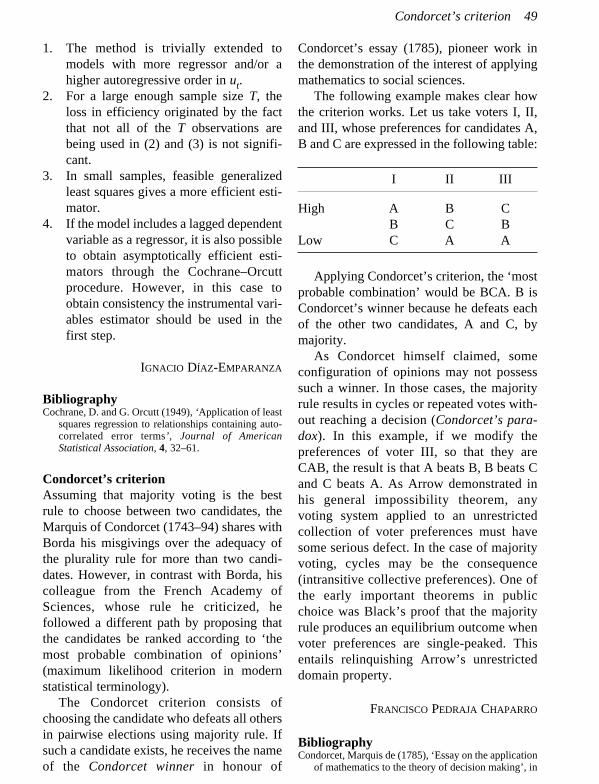
1. The method is trivially extended tomodels with more regressor and/or ahigher autoregressive order in ut.

2. For a large enough sample size T, theloss in efficiency originated by the factthat not all of the T observations arebeing used in (2) and (3) is not signifi-cant.

3. In small samples, feasible generalizedleast squares gives a more efficient esti-mator.

4. If the model includes a lagged dependentvariable as a regressor, it is also possibleto obtain asymptotically efficient esti-mators through the Cochrane–Orcuttprocedure. However, in this case toobtain consistency the instrumental vari-ables estimator should be used in thefirst step.

IGNACIO DÍAZ-EMPARANZA

BibliographyCochrane, D. and G. Orcutt (1949), ‘Application of least

squares regression to relationships containing auto-correlated error terms’, Journal of AmericanStatistical Association, 4, 32–61.

Condorcet’s criterionAssuming that majority voting is the bestrule to choose between two candidates, theMarquis of Condorcet (1743–94) shares withBorda his misgivings over the adequacy ofthe plurality rule for more than two candi-dates. However, in contrast with Borda, hiscolleague from the French Academy ofSciences, whose rule he criticized, hefollowed a different path by proposing thatthe candidates be ranked according to ‘themost probable combination of opinions’(maximum likelihood criterion in modernstatistical terminology).

The Condorcet criterion consists ofchoosing the candidate who defeats all othersin pairwise elections using majority rule. Ifsuch a candidate exists, he receives the nameof the Condorcet winner in honour of

Condorcet’s essay (1785), pioneer work inthe demonstration of the interest of applyingmathematics to social sciences.

The following example makes clear howthe criterion works. Let us take voters I, II,and III, whose preferences for candidates A,B and C are expressed in the following table:

I II III

High A B CB C B

Low C A A

Applying Condorcet’s criterion, the ‘mostprobable combination’ would be BCA. B isCondorcet’s winner because he defeats eachof the other two candidates, A and C, bymajority.

As Condorcet himself claimed, someconfiguration of opinions may not possesssuch a winner. In those cases, the majorityrule results in cycles or repeated votes with-out reaching a decision (Condorcet’s para-dox). In this example, if we modify thepreferences of voter III, so that they areCAB, the result is that A beats B, B beats Cand C beats A. As Arrow demonstrated inhis general impossibility theorem, anyvoting system applied to an unrestrictedcollection of voter preferences must havesome serious defect. In the case of majorityvoting, cycles may be the consequence(intransitive collective preferences). One ofthe early important theorems in publicchoice was Black’s proof that the majorityrule produces an equilibrium outcome whenvoter preferences are single-peaked. Thisentails relinquishing Arrow’s unrestricteddomain property.

FRANCISCO PEDRAJA CHAPARRO

BibliographyCondorcet, Marquis de (1785), ‘Essay on the application

of mathematics to the theory of decision making’, in

Condorcet’s criterion 49

K.M. Baker (ed.) (1976), Condorcet: SelectedWritings, Indianapolis, IN: Bobbs-Merrill.

See also: Arrow’s impossibility theorem, Borda’s rule.

Cournot aggregation conditionThis is a restriction on the derivative of alinear budget constraint of a householddemand system with respect to prices. It isthe expression of the fact that total expendi-ture cannot change in response to a change inprices.

Let us consider a static (one time period)model. Assume rational consumers in thesense that the total budget (denoted by x) isspent on different goods. This implies

x = ∑Nk=1

pkqk,

where qk denotes quantity and pk denotesprices.

Let us assume that a demand functionexists for each good k. These demands can bewritten as functions of x and the differentprices

qi = gi(x, p) for i = 1, . . . N,

where p is the N × 1 vector of prices. Theserelationships are called ‘Marshallian demandfunctions’, representing household con-sumption behaviour. Substituting thesedemand functions into the budget constraintgives

∑Nk=1

pkqk(x, p) = x.

This equation is referred to as the ‘adding-uprestriction’. Assume that the demand func-tions are continuous and differentiable. Theadding-up restriction can be expressed asrestriction on the derivatives of the demandfunctions, rather than on the functions them-selves. Specifically, total differentiation ofthe adding-up restriction with respect to prequires that

∂gk∑Nk=1

pk —— + qi = 0,∂pi

if the adding-up restriction is to continue toapply. This is termed the ‘Cournot aggrega-tion condition’ in honour of the French econ-omist A. Cournot (1801–77).

The Cournot condition can be rewritten interms of the elasticity of demand with respectto prices, as follows:

∑Nk=1wkeki

+ wi = 0,

where wk is the share of good k in theconsumer’s total budget and eki is theuncompensated cross-price elasticity. Thisrestriction is very useful for empiricalwork. The estimation of demand systems isof considerable interest to many problems,such as for the estimation of the incidenceof commodity and income taxes, for testingeconomic theories of consumer/householdbehaviour, or to investigate issues regard-ing the construction of consumer priceindices. One could test the theory ofdemand by seeing whether the estimatessatisfy the Cournot aggregation condition.Alternatively, this assumption of thedemand theory can be imposed a priori onthe econometric estimates, and statisticaltests can be used to test its validity.

RAQUEL CARRASCO

BibliographyNicholson, J.L. (1957), ‘The general form of the adding-

up criterion’, Journal of the Royal StatisticalSociety, 120, 84–5.

Worswick, G.D.N. and D.G. Champernowne (1954), ‘Anote on the adding-up criterion’, Review ofEconomic Studies, 22, 57–60.

See also: Marshallian demand function.

50 Cournot aggregation condition

Cournot’s oligopoly modelIn oligopoly theory we often assume thatfirms are Cournot competitors, or that firmscompete à la Cournot. This term originatesfrom the work of Augustin Cournot (1801–77) in 1838. The model presented in hisbook, after analyzing the pricing and produc-tion decisions of a monopolist, is extended toaccommodate the existence of more than onefirm and the strategic interaction amongthem.

The assumption is that firms competing inthe market offered a fixed quantity at anyprice. Firms choose simultaneously and takethe quantity of the other firms as exogenous.For a given total production, an auctioneerequates supply and demand, deriving theequilibrium price from this relationship. Thisprice, p, can be written as

p – ci(qi) qi/Q———— = —— ,

p h

where ci(qi) is the marginal cost for firm i ofproducing qi units, Q is the total productionof all firms and h is the elasticity of demandevaluated when total production is Q. Thisequation can be rewritten after aggregatingfor all firms as

n

p – ∑(qi/Q)ci(qi)i=1 HHI

——————— = —— ,p h

where n is the number of firms and HHI is theHerfindahl–Hirschman concentration index,computed as HHI = ∑n

i=1(qi/Q)2. Hence theCournot model predicts that more concentra-tion or a lower elasticity of demand results inan increase in the percentage margin of firms.In the limit, when concentration is maximumand only one firm produces, the index is HHI= 1, and consistently the price corresponds tothe monopoly one. In perfect competitionHHI = 0, and the price equals marginal cost.

This model went unnoticed until a firstreference by Joseph Bertrand in 1883.Bertrand criticizes the assumption that firmspost quantities instead of prices. Moreover, iffirms compete in prices, also known as à laBertrand, and the marginal cost is constantand equal for all firms, the unique equilib-rium corresponds to all firms producing atprice equal to marginal cost. In other words,two firms would be enough to achieve thecompetitive outcome. Moreover, dependingon the assumptions on cost, the equilibriummight be non-existent or multiple.

Although economists are mainly sympa-thetic to Bertrand’s idea that firms chooseprices rather than quantities, there is alsosome consensus that the predictions of theCournot model are more coherent withempirical evidence. For this reason an exten-sive literature has focused on reconciling thetwo points of view.

In the case of monopoly, the outcome isindependent of whether we assume that thefirm chooses a price or a quantity. In oligop-oly, however, an assumption on the residualdemand that a firm faces for a given actionby the other firms is required. In the Bertrandmodel the firm with the lowest price isassumed to produce as much as is necessaryto cover the total market demand. Thereforethe residual demand of any firm with ahigher price is 0. At the opposite end, theCournot model assumes that the quantityposted by each firm is independent of theprice. Moreover, each firm assumes thatconsumers with the highest valuation areserved by its competitors. This is what isdenoted as efficient rationing. For thisreason, the residual demand is the originaldemand where the quantity posted by otherfirms is subtracted. As a result, each firm is amonopolist of his residual demand.

Between these two competition choices avariety of other outcomes can be generated.If, for example, firms post supply functionsas in Klemperer and Meyer (1989), the

Cournot’s oligopoly model 51

multiplicity of equilibria includes both theBertrand and the Cournot outcomes asextreme cases.

In general, whether the outcome resem-bles the Cournot equilibrium or not willdepend on the relevant strategic variable ineach case. For example, Kreps andScheinkman (1983) study the case wherecapacity is fixed in the short run. In theirmodel, firms play in two stages. In the first,they simultaneously choose capacity, whilein the second they compete à la Bertrand.Despite the choice of prices the equilibriumcorresponds to the Cournot outcome. Theintuition is that, in the last stage, the capacityis fixed and each firm becomes a monopolistof the residual demand once the other firmhas sold its production. Other papers such asHolt and Scheffman (1987) show that most-favored-customer clauses also give rise toCournot outcomes.

Finally, another reason why the Cournotmodel has been widely used is that it is aprototypical example in game theory. Itderived reaction functions and a notion ofequilibrium later formalized by Nash. Inrecent years, it has also been used as an illus-tration of supermodular games.

GERARD LLOBET

BibliographyCournot, A.A. (1838), Recherches sur les principes

mathématiques de la théorie des richesses, Paris: L.Hachette.

Holt C. and D. Scheffman (1987), ‘Facilitating prac-tices: the effects of advance notice and best-pricepolicies’, Rand Journal of Economics, 18, 187–97.

Klemperer, P.D. and M.A. Meyer (1989), ‘Supply func-tion equilibria in oligopoly under uncertainty’,Econometrica, 57 (6), 1243–77.

Kreps, D. and J. Scheinkman (1983), ‘Quantity precom-mitment and Bertrand competition yield Cournotoutcomes’, Bell Journal of Economics, 14, 326–37.

Vives, X. (1989), ‘Cournot and the oligopoly problem’,European Economic Review, 33, 503–14.

See also: Bertrand competition model, Edgewortholigopoly model, Herfindahl–Hirschman index,Nash equilibrium.

Cowles CommissionThe Cowles Commission for Research inEconomics was set up to undertake econo-metric research in 1932 by Alfred Cowles(1891–1984), president of Cowles & Co., aninvesting counselling firm in ColoradoSprings, interested in the accuracy of fore-casting services, especially after the stockmarket crash in 1929. The Commissionstemmed from an agreement betweenCowles and the Econometric Society, createdin 1930, in order to link economic theory tomathematics and statistics, particularly intwo fields: general equilibrium theory andeconometrics. Its first home was ColoradoSprings under the directorship of Charles F.Roos, one of the founders of the EconometricSociety, but after his resignation the remote-ness of Colorado suggested a move. Thedecision of moving to Chicago in 1939, inspite of the interest of other universities, wasassociated with the appointment of TheodoreO. Yntema as the new research director.Later, under the directorship of Tjalling C.Koopmans, and as the opposition by theDepartment of Economics at Chicagobecame more intense, the Commissionmoved again, to Yale University in 1955.

The change of the Commission’s originalmotto ‘Science is Measurement’ to ‘Theoryand Measurement’ in 1952 reflected themethodological debates at the time. FrankKnight and his students, including MiltonFriedman and Gary Becker, criticized theCommission (Christ, 1994, p. 35). Friedmanargued against the econometric brand notonly because of the econometric methods butalso because of his skeptical view of theKeynesian model and consumption function.There were also financial considerations, anddifficulties in finding a new director ofresearch after Koopmans, who was involvedin the discussion, left. Once in Yale, JamesTobin, who had declined the directorship ofthe Commission at Chicago, accepted theappointment at Yale (Hildreth, 1986, p.11).

52 Cowles Commission

Numerous Cowles associates have wonNobel Prizes for research done while at theCowles Commission: Koopmans, Haavelmo,Markowitz, Modigliani, Arrow, Debreu,Simon, Klein and Tobin.

MARÍA BLANCO GONZÁLEZ

BibliographyChrist, Carl (1994), ‘The Cowles Commission’s contri-

butions to Econometrics at Chicago, 1939–1955’,Journal of Economic Literature, 32, 30–59.

Hildreth, Clifford (1986), The Cowles Commission inChicago 1939–1955, Berlin: Springer-Verlag.

Klein, Lawrence (1991), ‘Econometric contributions ofthe Cowles Commission, 1944–1947’, BancaNazionale del Lavoro Quarterly Review, 177,107–17.

Morgan, Mary (1990), History of Econometric Ideas,Cambridge: Cambridge University Press.

Cox’s testIn applied econometrics, frequently, there isa need for statistical procedures in order tochoose between two non-nested models.Cox’s test (Cox, 1961, 1962) is a related setof procedures based on the likelihood ratiotest that allows us to compare two competingnon-nested models.

In the linear hypothesis framework forlinear statistical models, consider the follow-ing two non-nested models:

H1 : Y = X1b1 + u1,H2 : Y = X2b2 + u2,

where u2 ~ N(0, s22 I).

These models are non-nested if the regres-sors under one model are not a subset of theother model even though X1 y X2 may havesome common variables. In order to test thehypothesis that X1 vector is the correct set ofexplanatory variables and X2 is not, Cox usedthe following statistic:

T sfl22C12 = — ln (————————————————)2 1sfl21 + — bfl1X�1 (I – X2(X�2X2)–1 X�2)X1bfl1T

T sfl22= — ln ( — ) .2 sfl221

Cox demonstrated that, when H1 is true,C12 will be asymptotically normallydistributed with mean zero and varianceV(C12). The small-sample distribution ofthe test statistic C12 depends on unknownparameters and thus cannot be derived.However, if we defined I – X2 (X�2X2)–1 X�2= M2 and we verified that M2 X1 = 0, thenthe models are nested and an exact testexist.

Given the asymptotic variance V(C12),under H1 true, the expression

C12————(V(C12))1/2

is asymptotically distributed as a standardnormal random variable.

Pesaran, in 1974, showed that, if theunknown parameters are replaced by consist-ent estimators, then

sfl21V fl(C12) = (——) bfl1X� M2M1M2Xbfl1

sfl412

can be used to estimate V(C12), where M2 isdefined as above and M1 = I – X (X�X)–1

X�. The test statistic can be run, under H1true, by using critical value from the stan-dard normal variable table. A large value ofC12 is evidence against the null hypothesis(H1).

NICOLÁS CARRASCO

BibliographyCox, D.R. (1961), ‘Test of separate families of hypothe-

sis’, Proceedings of the Fourth Berkeley Symposiumon Mathematical Statistics and Probability, vol. 1,Berkeley: University of California Press.

Cox, D.R. (1962), ‘Further results on tests of separatefamilies of hypothesis’, Journal of the RoyalStatistical Society, B, 24, 406–24.

Cox’s test 53

Davenant–King law of demandEmpirical study of the inverse relationshipbetween price and quantity. CharlesDavenant (1656–1714) and Gregory King(1648–1712) were two British mercantilistswho, as followers of William Petty’s ‘poli-tical arithmetic’, concerned themselveswith quantifying his statements. The formerwas a public servant and member of parlia-ment (MP) who, amongst other writings ontrade, wrote An Essay on Ways and Meansof Supplying the War (1695), Essay on theEast-India Trade (1696) and Discourses onthe Public Revenue and on the Trade ofEngland (1698). The works of the latterwere published in 1802, long after hisdeath, and in these appear a number ofinteresting estimates of population andnational income. King (1696) and Davenant(1699), the latter including extracts fromthe former, establish the inverse relation-ship between the amount of a goodproduced and its price. King shows that areduction in the wheat harvest may beaccompanied by an increase in its price inthe following proportions:

Reduction of harvest Increase in price

1 | 10 3 | 102 | 10 8 | 103 | 10 16 | 104 | 10 28 | 105 | 10 45 | 10

Davenant, in his work of 1699, states:

We take it, That a Defect in the Harvest mayraise the Price of Corn in the followingProportions:

Defect above the Common Rate

1 tenth 3 tenths2 tenths 8 tenths3 tenths } Raises the Price { 1.6 tenths4 tenths 2.8 tenths5 tenths 4.5 tenths

So that when Corn rises to treble theCommon Rate, it may be presumed, that wewant above a third of the Common Produce;and if we should want 5 Tenths, or half theCommon Produce, the Price would rise to nearfive times the Common Rate (Davenant [1699]1995, p. 255).

Later economists such as Arthur Young,Dugald Stewart, Lord Lauderdale, WilliamStanley Jevons, Philip Henry Wicksteed,Alfred Marshall and Vilfredo Pareto werefamiliar with King’s or Davenant’s exposé,or their joint work when they developed theirtheory of demand.

LUIS PERDICES DE BLAS

BibliographyCreedy, John (1987), ‘On the King–Davenant “law” of

demand’, Scottish Journal of Political Economy, 33(3), 193–212.

Davenant, Charles (1699), An Essay Upon the ProbableMethods of Making a People Gainers in the Balanceof Trade, reprinted in L. Magnusson (ed.) (1995),Mercantilism, vol. III, London and New York:Routledge.

Endres, A.M. (1987), ‘The King–Davenant “law” inclassical economics’, History of Political Economy,19 (4), 621–38.

King, Gregory (1696), Natural and Political Ob-servations and Conclusions upon the State andCondition of England, reprinted in P. Laslett (1973),The Earliest Classics: John Graunt and GregoryKing, Farnborough, Hants: Gregg InternationalPublishers.

Díaz-Alejandro effectThis refers to the paradox that a devaluationmay lead to a decrease in domestic output as

54

D

a consequence of its redistributive effects.This runs counter to the conventional text-book view that devaluations, by encouragingthe production of tradable goods, will beexpansionary. To understand the effect,assume, for instance, that a country isdivided into two classes – wage earners andcapitalists – with each class made up of indi-viduals with identical tastes. Since the capi-talists’ marginal propensity to consume willpresumably be lower than the workers’, theredistribution of income from wage earnersto capitalists brought about by a devaluationwill have a contractionary effect on aggre-gate demand, thereby reducing aggregateoutput. This contraction will run parallel tothe improvement in the trade balance.

When the effect was formulated in 1963,the redistributive effect of devaluations wasalready well known. But Cuban economistCarlos F. Díaz-Alejandro (1937–85) empha-sized the significance and timing of the effect,and its impact on domestic output. He basedhis insight on the experience of devaluationsin Argentina and other semi-industrializedcountries during the 1950s, where devalu-ations had implied a significant transfer ofresources from urban workers to landowners.

A review of the literature on this and othereffects of devaluations can be found inKamin and Klau (1998).

EMILIO ONTIVEROS

BibliographyDíaz-Alejandro, Carlos F. (1963), ‘A note on the impact

of devaluation and the redistributive effect’, Journalof Political Economy, 71 (6), 577–80

Kamin, Steven B. and Marc Klau (1998), ‘Some multi-country evidence on the effects of real exchangerates on output’, Board of Governors of the FederalReserve System, International Finance DiscussionPapers, no. 611, May.

Dickey–Fuller testTo apply standard inference procedures in adynamic time series model we need the vari-ous variables to be stationary, since the bulk

of econometric theory is built upon theassumption of stationarity. However, inapplied research we usually find integratedvariables, which are a specific class of non-stationary variables with important economicand statistical properties. These are derivedfrom the presence of unit roots which giverise to stochastic trends, as opposed to puredeterministic trends, with innovations to anintegrated process being permanent insteadof transient.

Statisticians have been aware for manyyears of the existence of integrated seriesand, in fact, Box and Jenkins (1970) arguethat a non-stationary series can be trans-formed into a stationary one by successivedifferencing of the series. Therefore, fromtheir point of view, the differencing opera-tion seemed to be a prerequisite for econo-metric modelling from both a univariate anda multivariate perspective.

Several statistical tests for unit rootshave been developed to test for stationarityin time series. The most commonly used totest whether a pure AR(1) process (with orwithout drift) has a unit root are theDickey–Fuller (DF) statistics. These teststatistics were proposed by Dickey andFuller (1979).

They consider the three following alterna-tive data-generating processes (DGP) of atime series:

yt = rnyt–1 + et (1)

yt = mc + rcyt–1 + et (2)

yt = mct + gt + rctyt–1 + et (3)

where et ~ iid(0, s2e), t is a time trend and the

initial condition, y0 is assumed to be a knownconstant (zero, without loss of generality).For equation (1), if rn < 1, then the DGP is astationary zero-mean AR(1) process and if rn= 1, then the DGP is a pure random walk. Forequation (2), if rc < 1, then the DGP is a

Dickey–Fuller test 55

stationary AR(1) process with mean mc/(1 –rc) and if rn = 1, then the DGP is a randomwalk with a drift mn. Finally, for equation (3),if rct < 1, the DGP is a trend-stationaryAR(1) process with mean

mct——— + gct∑t

j=0[rjct(t – j)]

1 – rct

and if rct = 1, then the DGP is a random walkwith a drift changing over time.

The test is carried out by estimating thefollowing equations

Dyt = (rn – 1)yt–1 + et (1�)

Dyt = b0c + (rc – 1)yt–1 + et (2�)

Dyt = b0ctt + b1ctt + (rct – 1)yt–1 + et (3�)

The tests are implemented through theusual t-statistic on the estimated (r – 1).They are denoted t, tm and tt, respectively.Given that, under the null hypothesis, thistest statistic does not have the standard tdistribution, Dickey and Fuller (1979) simu-lated critical values for selected sample sizes.More extensive critical values are reportedby MacKinnon (1991).

Hitherto, we have assumed that the DGPis a pure AR(1) process. If the series is corre-lated at higher order lag, the assumption ofwhite noise disturbance is violated. Dickeyand Fuller (1979) have shown that we canaugment the basic regression models(1�)–(3�) with p lags of Dyt:

p

Dyt = (rn – 1)yt–1 + ∑aiDyt–i + et (1�)i=1

p

Dyt = b0c + (rc – 1)yt–1 + ∑aiDyt–i + et (2�)i=1

Dyt = b0ctt + b1ctt + (rct – 1)yt–1p

+ ∑aiDyt–i + et (3�)i=1

The tests are based on the t-ratio on (rfl – 1)and are known as ‘augmented Dickey–Fuller’ (ADF) statistics. The critical valuesare the same as those discussed for the DFstatistics, since the asymptotic distributionsof the t-statistics on (rfl – 1) is independent ofthe number of lagged first differencesincluded in the ADF regression.

SIMÓN SOSVILLA-ROMERO

BibliographyBox, G.E.P. and G.M. Jenkins (1976), Time Series

Analysis: Forecasting and Control, rev. edn,Holden-Day.

Dickey, D.A. and W.A. Fuller (1979), ‘Distribution ofthe estimators for autoregressive time series with aunit root’, Journal of the American StatisticalAssociation, 74, 427–31.

MacKinnon, J.G. (1991), ‘Critical values for cointegra-tion tests’, Chapter 13 in R.F. Engle and C.W.J.Granger (eds), Long-run Economic Relationships:Readings in Cointegration, Oxford University Press.

See also: Box-Jenkins Analysis, Phillips–Perron test.

Director’s lawThis is an empirical proposition about theoverall effect of government policies on thepersonal distribution of income. Namedafter Aaron Director, (1901–2004) Professorof Economics at the Law School of theUniversity of Chicago, it states that, nomatter how egalitarian their aims might be,the net effect of government programs is toredistribute income toward the middle class.True to the spirit of the Chicago School andits reliance on the oral tradition, AaronDirector never got to publish his reflectionson the positive economics of income redis-tribution or, indeed, on many other subjects.It is chiefly through his influence on hiscolleagues and students that his contribu-tions are known. Milton Friedman, GeorgeStigler and others have repeatedly acknowl-edged their indebtedness to Director’s inspi-ration and criticism.

Stigler, who coined the law, was, morethan any other, responsible for bringing

56 Director’s law

Director’s views on redistribution to theattention of the economics profession.Director challenged what is still the domi-nant view, according to which the progres-sive income tax and income transfer schemesthat figure so prominently in modern fiscalsystems effectively operate a redistributionof income from the wealthy to the poorestmembers of society. He pointed out, accord-ing to Stigler, several features of contem-porary democracies that account for theunconventional result that governmentsredistribute income from the tails to themiddle of the distribution.

Firstly, under majority voting, in the zero-sum game of cash income redistribution, theminimum winning coalition would comprisethe lower half of the distribution. Secondly,one should notice that, as the very poor anddestitute do not exercise their voting rights asmuch as the average citizen, middle-incomevoters would be overrepresented in thewinning coalition. Thirdly, and more rele-vant, modern governments not only effectpure cash transfers but mostly engage in avariety of actions in response to the pressuresof organized interest groups that end uptransferring income to the middle class.Agricultural policy transfers income to farm-ers and affluent landowners; public educa-tion (particularly higher education) is atransfer to the well-to-do; subsidies toowner-occupied housing likewise benefitthose who are well off; minimum wage legis-lation favours the lower middle class at theexpense of the very poor; professional licens-ing erects barriers against the most enterpris-ing but less fortunate citizens; lastly, evenmost programs focused on poverty allevi-ation, by enlisting the cooperation of socialworkers, health experts and government offi-cials, create a derived demand for servicesprovided mainly by members of the middleclass.

ALFONSO CARBAJO

BibliographyRiker, W.H. (1962), The Theory of Political Coalitions,

New Haven: Yale University Press.Stigler, G.J. (1970), ‘Director’s law of public income

redistribution’, Journal of Law and Economics, 13(1), 1–10.

Tullock, G. (1971), ‘The charity of the uncharitable’,Western Economic Journal, 9 (4), 379–92.

Divisia indexThe French statistician François Divisia(1889–1964) formulated in a long articlepublished in 1925–6 a new type of index thattried to measure the amount of money heldfor transaction purposes as an alternative toother indexes, based on the conventionalsimple-sum aggregates.

Assume that an individual spends a totalamount e(t) buying n goods in quantities(x1(t), . . ., xn(t)) at prices (p1(t), . . ., pn(t)) inperiod t. Therefore

n

e(t) = ∑pi(t)xi(t).i=1

Total log-differentiation of e(t) gives

e(t) n pi(t)xi(t) p˘i(t) n pi(t)xi(t) x˘i(t)—— = ∑———— —— + ∑———— ——, (1)e(t) i=1 e(t) pi(t) i=1 e(t) xi(t)

where dots over variables indicate derivativeswith respect to time. The left side of (1) is theinstant growth rate of expenditure and isdecomposed into two components: (a) theDivisia index of prices which is the first termof the right-hand side of (1), and (b) theDivisia index of quantities which is the secondterm of the right-hand side of (1). Thereforethe Divisia indexes are weighted averages ofthe growth rates of individual prices (or quan-tities), the weight being the respective sharesin total expenditure. Although the indexes in(1) are expressed in continuous time, whichmade them inappropriate for empirical analy-sis, Törnqvist (1936) solved the problem forapproximating (1) to discrete time terms.Törnqvist’s solution in the case of prices is

Divisia index 57

n 1 pi(t)xi(t) pi(t – 1)xi(t – 1)∑ — [———— + ———————] ×i=1 2 e(t) e(t – 1)

[log pi(t) – log pi(t – 1)],

which means that the growth rate of prices isapproximated by the logarithmic differencesand the weights are approximated by simpleaverages between two consecutive periods.In the same applied vein, the Divisia indexescan be considered as ‘chain indexes’ and wecan approximate them for Laspeyres orPaasche indexes which change their base inevery period.

Although the Divisia indexes have beenused in theoretical work for many differentproblems (industrial and consumption prices,quantities, cost of living and so on) theyaimed at avoiding the inconvenience of othermonetary aggregates computed as simplesums of components of the monetary quanti-ties, such as currency and demand deposits.That implies perfect substitutability betweencomponents of the monetary aggregate,whereas they are not equally useful for alltransactions. Therefore simple sum aggrega-tion is inappropriate in consumer demandtheory.

Instead of measuring the stock of moneyheld in the economy, the Divisia indexassesses the utility the consumer derivesfrom holding a portfolio of different mon-etary assets. It treats monetary assets asconsumer durables such as cars, televisionsand houses, yielding a flow of monetaryservices. These services are performed bydifferent monetary assets to a differentdegree and are proportional to the stock ofmonetary assets held. If the consumer’s util-ity function is weakly separable in consump-tion and monetary assets, the Divisiaaggregate can be regarded as a singleeconomic good.

In brief, the objective of the Divisiameasure is to construct an index of the flowof monetary services from a group of mon-

etary assets that behave as if they were a singlecommodity. Divisia monetary aggregates arethus obtained by multiplying each componentasset’s growth rate by its share weights andadding the products. Every component’s shareweight depends on the user costs and the quan-tities of all components assets.

Divisia monetary aggregates can beapplied when analysing whether structuralchange affects the stability of the demand-for-money and supply-of-money functions,under total deregulation and is a good indi-cator of control on money supply.

MILAGROS AVEDILLO

BibliographyBernett, W.A. (1980), ‘Economic monetary aggregates:

an application of index number and aggregationtheory’, Journal of Econometrics, 14, 11–48.

Divisia, F. (1925–6), ‘L’indice monétaire de la théoriede la monnaie’, Revue d’Economie Politique, 39 (4),980–1008; 39 (6), 1121–51; 40 (1), 49–81.

Törnqvist, L. (1936), ‘The Bank of Finland’s consump-tion price index’, Bank of Finland Monthly Review,10, 1–8.

See also: Laspeyres index, Paasche index.

Dixit–Stiglitz monopolistic competitionmodelThe model of Avinash K. Dixit and Joseph E.Stiglitz (1977) (DS hereafter) is a benchmarkmonopolistic competition model which hasbeen widely used in several economic areassuch as international economics, growtheconomics, industrial organization, regionaland urban economics and macroeconomics.

The DS model and the similar Spence(1976) model introduced an alternative wayto treat product differentiation. In the hori-zontal and vertical differentiation models aproduct competes more with some productsthan with others. In the DS and the Spencemodels there are no neighboring goods: allproducts are equally far apart, so every onecompetes with the rest. This hypothesisrequires defining the industry appropriately.

58 Dixit–Stiglitz monopolistic competition model

Products must be good substitutes amongthemselves, but poor substitutes for the othercommodities in the economy. Additionally,the preference structure allows modelingdirectly the desirability of variety, using theconvexity of indifference surfaces of aconventional utility function. The representa-tive consumer will purchase a little bit ofevery available product, varying the propor-tion of each according to their prices.

The main characteristics of this model arethe following. First, there is a representativeconsumer whose utility function depends onthe numeraire commodity, labelled 0, and onall the n commodities of a given industry orsector. The numeraire aggregates the rest ofthe economy. Using x0 and xi, i = 1, 2 . . ., n,to denote the amount of the commodities, theutility function will be

u = U(x0, V(x1, x2, . . ., xn)),

where U is a separable and concave function,and V is a symmetric function. In particular,the central case developed by DS is theconstant-elasticity (CES) case, in which

n 1/r

V(x1, x2, . . ., xn) = (∑xri ) , 0 < r < 1

i=1

and U is assumed homothetic in its argu-ments. This implies assuming that the sectorexpands in proportion to the rest of the econ-omy as the size of the economy changes,which can be very useful in internationaltrade and growth theory. Alternatively, in theSpence model, V is assumed CES and Uquasi-linear, which can be very convenient inthe context of partial equilibrium analysis.

Second, the consumer budget constraint is

n

xo + ∑ pixi = I,i=1

where I is the income and pi is the price ofcommodity i.

Third, there are n different firms withidentical cost functions. Each firm must facesome fixed set-up cost and has a constantmarginal cost.

Fourth, each firm produces a differentcommodity.

Fifth, the number of firms, n, is reason-ably large and accordingly each firm is negli-gible, in the sense that it can ignore its impacton, and hence reactions from, other firms,and the cross-elasticity of demand is negli-gible. In the CES case, for each commodity iit can be checked that demand will be givenby xi = yqs pi

–s, where s = 1/(1 – r) is theelasticity of substitution between the differ-entiated products and y and q are quantityand price indices

n 1/r n 1/(1–s)

y = (∑xri ) , q = (∑pi

1–s)1/(1–s).i=1 i=1

Assuming that each firm is negligible impliesthat ∂logq/∂logpi and ∂logxi/∂logpj, ∀ i ≠ j,both depending on a term of order 1/n, arenegligible.

Finally, firms maximize profits and entryis free.

Monopolistic competition is characterizedby solving the representative consumer prob-lem to obtain demand functions, by solvingthe firm’s problems to determine prices, andby taking into account that entry will proceeduntil the next potential entrant would make aloss.

DS use their model to analyze the optimal-ity of the market solution in the monopolisticequilibrium addressing the question of quan-tity versus diversity, but their model has beenused in a vast number of papers with the mostvaried purposes. In a collection of essaysedited by Brakman and Heijdra (2003),several authors, including Dixit and Stiglitz,present their reflections on the actual state ofthe theory of monopolistic competition.

CONSUELO PAZÓ

Dixit–Stiglitz monopolistic competition model 59

BibliographyBrakman, S. and B.J. Heijdra (eds) (2003), The

Monopolistic Competition Revolution in Retrospect,Cambridge University Press.

Dixit, A.K. and J.E. Stiglitz (1977), ‘Monopolisticcompetition and optimum product diversity’,American Economic Review, 67 (3), 297–308.

Spence, A.M. (1976), ‘Product selection, fixed costs andmonopolistic competition’, Review of EconomicStudies, 43, 217–35.

See also: Chamberlin’s oligopoly model.

Dorfman–Steiner conditionIn their seminal paper on advertising,Robert Dorfman (1916–2002) and Peter O.Steiner show that a profit-maximizing firmchooses the advertising expenditure andprice such that the increase in revenueresulting from one additional unit of adver-tising is equal to the price elasticity ofdemand for the firm’s product. This resulthas usually been formulated in terms ofadvertising intensity, the ratio of advertisingexpenditure to total sales. For this ratio theformula of the Dorfman–Steiner conditionis

s h—— = —,pq e

where s denotes the total expenses of adver-tising, p is the price, q is the quantity, h isthe demand elasticity with respect to adver-tising expenditures and e is the price elastic-ity of demand. The equation states that themonopolist’s optimal advertising to salesratio is equal to the relationship between theadvertising elasticity of demand and theprice elasticity of demand. To obtain thecondition two assumptions are required: onthe one hand, the demand facing the firm hasto be a function of price and advertising and,on the other hand, the cost function has to beadditive in output and advertising.

JOSÉ C. FARIÑAS

BibliographyR. Dorfman and P.O. Steiner (1954), ‘Optimal advertis-

ing and optimal quality’, American EconomicReview, 44 (5), 826–36.

Duesenberry demonstration effectIn February 1948, James S. Duesenberry(b.1918) presented his doctoral dissertationin the University of Michigan, titled ‘TheConsumption Function’, whose contentswere later published with the title Income,Saving and the Theory of ConsumerBehavior (1949) that was the starting pointfor the behavior analyses related to consump-tion and saving until the introduction of theapproaches associated with the concepts ofpermanent income and life cycle.

The expression ‘demonstration effect’ isspecifically stated in section four of the thirdchapter of the above-mentioned book. Thisexpression overcame the absolute incomeapproach. In this approach the utility indexwas made dependent on current and futureconsumption and wealth, but this index waspeculiar to every individual and independentof the others. On the contrary, the demon-stration effect rejects both the independencebetween individuals and the temporalreversibility of the decisions taken. It formsthe basis of the explanation of the behavior inthe interdependence of individuals and theirreversible nature of their temporal deci-sions.

Thus, on the one hand, it is accepted thatindividuals aspire to consume better qualitygoods and in larger quantities when theirincome increases, but, on the other hand, theutility index of any individual does notdepend on the absolute level of theirconsumption, but on the relation betweentheir expenses and other people’s expensesand, taking into account the time dimension,the attitudes towards their future spendingwill depend on the current levels ofconsumption, and especially on the maxi-mum level that was previously reached.

60 Dorfman–Steiner condition

What was regarded as the ‘fundamentalpsychological law’, namely, every increasein income entails an increase in consumptionin a ratio less than the unit, is replaced byanother ‘psychological postulate’ that statesthat it is more difficult for a family to reduceits expenses from a high level than to refrainfrom spending big amounts for the first time.Starting from those assumptions, severalconclusions can be drawn.

1. The increases in income in the wholepopulation, without altering the distribu-tion, will not alter the average consump-tion.

2. On the contrary, the increases in incomein a certain sector of the population willtend to increase consumption in terms ofits absolute value but to decrease aver-age consumption.

3. This last effect is more noticeable in thehigh-income group (but this is not validin the low-income groups, where thetendency to consumption is the unit).

4. Changes in the income distribution and/orthe population pyramid will affect theperformance of consumption and saving.

5. A steady increase in income over timeyields, as a result, an average tendencytowards stable consumption.

6. A deceleration in economic activity willcause an increase in the averagetendency to consume, which will put abrake on the depression.

The demonstration effect also has strongimplications for the welfare state since theindividual welfare indices will depend (posi-tively or negatively) on incomes and lifestandards of others. All this alters the effi-ciency criteria in economic analysis as wellas the allocation and fairness criteria, and thefiscal mechanisms required to rectify theinequalities arising from the efficiency crite-ria based on the strict independence betweenindividuals.

Finally, the demonstration effect shows aconsiderable explanatory power in relation tothe introduction of new goods in the marketand the development and structure of thetotal amount of spending.

JON SANTACOLOMA

BibliographyDuesenberry, J.S. (1949), Income, Saving and the

Theory of Consumer Behavior, Cambridge, MA:Harvard University Press.

Durbin–Watson statisticThis determines whether the disturbanceterm of a regression model presents autocor-relation according to a first-order autoregres-sive scheme –AR(1)–. Its numerical value(which may range from zero to four, bothinclusive) is obtained from the residuals (et)of the estimation by ordinary least squares ofthe model. So an expression from which itcan be obtained is given by

T

∑(et – et–1)2

t=2DW = —————.

T

∑e2t

t=1

Values near zero indicate that the disturbanceterm presents autocorrelation according to ascheme AR(1) with positive parameter (r1);values near four indicate that the disturbanceterm presents autocorrelation according to ascheme AR(1) with negative parameter (r1);and values near two indicate that the distur-bance term does not present autocorrelationaccording to a scheme AR(1). Accordingly,one can obtain an approximate value for theDurbin–Watson statistic by means of theexpression: DW = 2(1 – rfl1), where rfl1 is theestimation of the parameter of the schemeAR(1). Among its drawbacks is the fact thatit should not be used if the delayed endog-enous variable is among the regressors

Durbin–Watson statistic 61

because in this case the conclusion tends tobe that the disturbance term does not presentautocorrelation according to a scheme AR(1).

JORDI SURINACH

BibliographyDurbin, J. and G.S. Watson (1950), ‘Testing for serial

correlation in least squares regression I’, Biometrika,37, 409–28.

Durbin, J. and G.S. Watson (1951), ‘Testing for serialcorrelation in least squares regression II’,Biometrika, 38, 159–78.

Durbin, J. and G.S. Watson (1971), ‘Testing for serialcorrelation in least squares regression III’,Biometrika, 58, 1–42.

Durbin–Wu–Hausman testThe Durbin–Wu–Hausman test (henceforthDWH test) has been developed as a specifi-cation test of the orthogonality assumption ineconometrics. In the case of the standardlinear regression model, y = Xb + u, thisassumption is that the conditional expecta-tion of u given X is zero; that is, E(u/X) = 0or, in large samples,

X�uplim —— = 0.

T

The DWH test relies on a quadratic formobtained from the difference between two

alternative estimators of the vector ofregression coefficients, say b fl0 and b fl1. b fl0must be consistent and (asymptotically)efficient under the null hypothesis, but it isinconsistent under the alternative hypoth-esis. On the other hand, b fl1 is not asymptot-ically efficient under the null hypothesisbut it is consistent under both the null and the alternative hypotheses. The DWH testis based on q fl = b fl1 – b fl0. Under the nullhypothesis, q fl converges in probability tozero while, under the alternative hypoth-esis, this limit is not zero. The idea that onemay base a test on the vector of differencesbetween two vectors of estimates datesback to Durbin (1954). Two other relevantpapers are Wu (1973) and Hausman (1978).In these papers, the approach is extended to a simultaneous equation econometricmodel.

ANTONIO AZNAR

BibliographyDurbin, J. (1954), ‘Errors in variables’, Review of the

International Statistical Institute, 22, 23–32.Hausman J.A. (1978), ‘Specification tests in economet-

rics’, Econometrica, 46, 1251–71.Wu, D.M. (1973), ‘Alternative tests of independence

between stochastic regressors and disturbances’,Econometrica, 41, 733–50.

62 Durbin–Wu–Hausman test

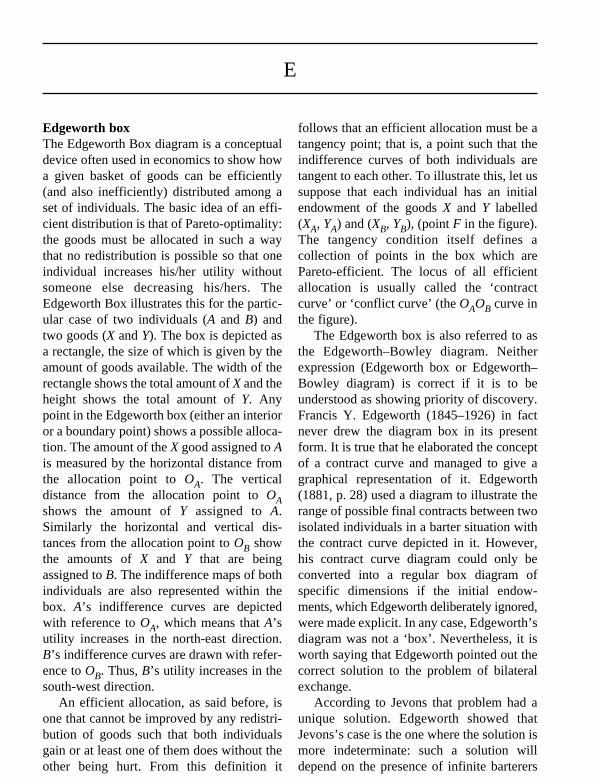
Edgeworth boxThe Edgeworth Box diagram is a conceptualdevice often used in economics to show howa given basket of goods can be efficiently(and also inefficiently) distributed among aset of individuals. The basic idea of an effi-cient distribution is that of Pareto-optimality:the goods must be allocated in such a waythat no redistribution is possible so that oneindividual increases his/her utility withoutsomeone else decreasing his/hers. TheEdgeworth Box illustrates this for the partic-ular case of two individuals (A and B) andtwo goods (X and Y). The box is depicted asa rectangle, the size of which is given by theamount of goods available. The width of therectangle shows the total amount of X and theheight shows the total amount of Y. Anypoint in the Edgeworth box (either an interioror a boundary point) shows a possible alloca-tion. The amount of the X good assigned to Ais measured by the horizontal distance fromthe allocation point to OA. The verticaldistance from the allocation point to OAshows the amount of Y assigned to A.Similarly the horizontal and vertical dis-tances from the allocation point to OB showthe amounts of X and Y that are beingassigned to B. The indifference maps of bothindividuals are also represented within thebox. A’s indifference curves are depictedwith reference to OA, which means that A’sutility increases in the north-east direction.B’s indifference curves are drawn with refer-ence to OB. Thus, B’s utility increases in thesouth-west direction.

An efficient allocation, as said before, isone that cannot be improved by any redistri-bution of goods such that both individualsgain or at least one of them does without theother being hurt. From this definition it

follows that an efficient allocation must be atangency point; that is, a point such that theindifference curves of both individuals aretangent to each other. To illustrate this, let ussuppose that each individual has an initialendowment of the goods X and Y labelled(XA, YA) and (XB, YB), (point F in the figure).The tangency condition itself defines acollection of points in the box which arePareto-efficient. The locus of all efficientallocation is usually called the ‘contractcurve’ or ‘conflict curve’ (the OAOB curve inthe figure).

The Edgeworth box is also referred to asthe Edgeworth–Bowley diagram. Neitherexpression (Edgeworth box or Edgeworth–Bowley diagram) is correct if it is to beunderstood as showing priority of discovery.Francis Y. Edgeworth (1845–1926) in factnever drew the diagram box in its presentform. It is true that he elaborated the conceptof a contract curve and managed to give agraphical representation of it. Edgeworth(1881, p. 28) used a diagram to illustrate therange of possible final contracts between twoisolated individuals in a barter situation withthe contract curve depicted in it. However,his contract curve diagram could only beconverted into a regular box diagram ofspecific dimensions if the initial endow-ments, which Edgeworth deliberately ignored,were made explicit. In any case, Edgeworth’sdiagram was not a ‘box’. Nevertheless, it isworth saying that Edgeworth pointed out thecorrect solution to the problem of bilateralexchange.

According to Jevons that problem had aunique solution. Edgeworth showed thatJevons’s case is the one where the solution ismore indeterminate: such a solution willdepend on the presence of infinite barterers

63

E

64

Segura – Edgeworth box

A1

B5 B4 B3

B2

F

B1

A2A3 A4 A5

G

XB OB

YB

XAOA

YA

Edgeworth box, or Edgeworth–Bowley diagram

in a setting of perfect competition, whichwill reduce the contract curve to a sole point.Irving Fisher was the first economistexpressly to employ a system of indifferencecurves for each person in 1892. Twenty oneyears later Pareto, in a work published inEncyklopädie der mathematischen Wissen-schaften, used a system of indifferencecurves (that is, indifference ‘maps’). Such asystem of curves is a necessary prerequisitefor developing the so-called ‘box diagram’.The Edgeworth box appeared for the firsttime in its present form in the 1906 edition ofPareto’s Manuale (p. 187). In 1924 ArthurBowley published the first edition of hisMathematical Groundwork (p. 5), whichcontained an elaborate version of the boxdiagram.

Given that Bowley’s book appeared a fewyears later than Pareto’s, the questionremains as to whether Bowley’s constructionwas in any sense autonomous. It is quite clearthat Bowley had already known Pareto’swritings, since he quotes Pareto in hisMathematical Groundwork. Bowley’s namecame to be associated with the box diagramprobably because Pareto was virtuallyunknown in the English-speaking worldbefore the 1930s, and this world becameacquainted with the box diagram throughBowley’s book. Therefore it is not surprisingthat, when Bowley popularized the contem-porary version of the box diagram to explaintwo-individual, two-commodity exchange,Edgeworth’s name became closely identifiedwith the device. From that moment on thisconceptual device has commonly been calledthe Edgeworth–Bowley box diagram.

ANGEL MARTÍN-ROMÁN

BibliographyBowley, Arthur L. (1924), The Mathematical

Groundwork of Economics, Oxford: The ClarendonPress.

Edgeworth, Francis Y. (1881), Mathematical Psychics,London: Kegan Paul.

Pareto, Vilfredo (1906), Manuale di economia politicacon una introduzione alla scienza sociale, Milan:Piccola Biblioteca Scientifica No. 13. English trans.by A.S. Schwier in A.S. Schwier and A.N. Page(eds) (1971), Manual of Political Economy, NewYork: A.M. Kelley.

Edgeworth expansionThe representation of one distribution func-tion in terms of another is widely used as atechnique for obtaining approximations ofdistributions and density functions.

The Edgeworth representation, introducedat the beginning of the twentieth century, andderived from the theory of errors, wasupdated by Fisher in 1937 through the use ofthe Fourier transform.

Let X be a standardized random variable,with density function f (x). Let f(x) be thedensity of the N(0, 1), let ki i = 3, 4, . . . be thecumulants of X. The Edgeworth expansion off(x) is

k3 k4f(x) = f(x)(1 + — H3(x) + — H4(x)

3! 4!

k5 10k3 + k6+ — H5(x) + ———— H6(x) +) . . .,

5! 6!

where the Hj are the Hermite polinomials oforder j = 3, 4, . . ., defined as functions of thederivative of the density f(x) by fk)(x) =(–1)kf(x)Hk(x), or equivalently by recursiveequations: Hk+1(x) = xHk(x) – kHk–1(x). Asfor the function distribution,

k3 k4F(x) = F(x) – — H2(x)f(x) – — H3(x)f(x)

3! 4!

k23

– — H5(x)f(x) + . . .,6!

where F(x) is the standard normal functiondistribution. In the case of independent andidentically distributed random variables Xiwith mean q0 and finite variance s2, thedistribution of the statistic

Edgeworth expansion 65

Sn = n1/2(X— – q0)/s

is asymptotically normal and has anEdgeworth expansion as a power series inn

–12:

–1

P(Sn ≤ x) = F(x) + n2p1(x)f(x) + n–1p2(x)f(x)

–j—

+ . . . + n2pj(x)f(x) + . . .,

where the pj are polynomials depending onthe cumulants of X and of the Hermite poly-nomials.

The essential characteristics of theEdge-worth expansion are, first, that it is an orthogonal expansion, due to thebiorthogonality between the Hermite poly-nomials and the derivatives of the normaldensity

∞

∫Hk(x)fm)(x)dx = (–1)mm!dkm,–∞

where dkm is the Kronecker delta; andsecond, that the coefficients decrease uni-formly.

As an application we emphasize its use inthe non-parametric estimation of densityfunctions and bootstrap techniques.

VICENTE QUESADA PALOMA

BibliographyKendall M. Stuart (1977), The Avanced Theory of

Statistics, vol. 1, London: Macmillan.

See also: Fourier transform.

Edgeworth oligopoly modelThe Francis I. Edgeworth (1845–1926)model (1897) merged the two main oligopo-listic behaviour models (quantity and pricecompetition models) by introducing capacity

constraints in a two-period game whichallowed firms to make decisions on bothquantity and price. His new approach to non-cooperative firm competition overcame thebasic limitations of previous models and setthe standard framework that has been used todevelop the oligopoly theory.

The quantity competition model (Cournot,1838) has been criticized for assuming thatfirms choose quantities produced and aneutral auctioneer chooses the price thatclears the market, which is seen as unrealis-tic. The price competition model (Bertrand,(1883) assumptions are more plausible, aswithin this model it is firms who choseprices, but it leads to the counterintuitiveBertrand paradox: only two firms are neededfor the competitive equilibrium to beachieved (marginal cost pricing and zeroprofits for all firms).

Edgeworth set a simple two-stage model. Instage one, firms select their production capac-ity (more capacity implies a larger fixed cost)and, in stage two, firms choose prices takinginto account that they cannot sell more thanthey are capable of producing. That is, we giveup Bertrand’s assumption that the firm offer-ing the lowest price covers the whole market.Moreover, the Edgeworth model captures thegeneral belief that price is the main instrumentthat a firm can change in the short run, whilecost structures and production levels can onlybe altered in the long run.

This model implies that a zero profit solu-tion no longer presents an equilibrium, and itresults in a solution with non-competitiveprices. The underlying argument is intuitive:since capacity investment is costly, no firmwill enter the market to make non-positiveprofits (or it will just select zero capacity).Thus it is obvious that the equilibrium solu-tion achieves the following: no firm overin-vests (in that case, a reduction in capacityinvestment would increase profits) and prof-its are, at least, as large as the fixed cost ofcapacity investment.

66 Edgeworth oligopoly model

To sum up, Edgeworth shows that quan-tity and price competition models can beintegrated in a general model that, dependingon the cost structure of a market, will lead toa solution close to Bertrand’s (industries withflat marginal costs) or Cournot’s (industrieswith rising marginal costs).

DAVID ESPIGA

BibliographyEdgeworth, F. (1897), ‘La teoria pura del monopolio’,

Giornale degli Economisti, 40, 13–31; translated as‘The theory of monopoly’ in Papers Relating toPolitical Economy (1925), vol. 1, 111–42, London:Macmillan.

See also: Bertrand competition model, Cournot’soligopoly model.

Edgeworth taxation paradoxFrancis Y. Edgeworth (1845–1926) de-scribed this paradox (1897a, 1897b) accord-ing to which the setting of a tax on goods orservices can lead to a reduction in theirmarket price under certain circumstances. Inits original formulation this result wasobtained for monopolies jointly producingsubstitute goods (for instance, first- andsecond-class railway tickets). It was subse-quently extended for complementary goods(that is, passenger transport and luggage forthe same example). Years later, Hotelling(1932) put forward a rigorous demonstrationthat extended these results to include cases offree competition and duopolies, and showedits verisimilitude for real scenarios that went further than the limitations imposed by partial equilibrium analyses and in theface of the resistance it initially aroused(Seligman, 1899), pp. 174, 191, 1921, p. 214,Edgeworth, 1899, 1910).

Also known as the ‘Edgeworth–Hotellingparadox’, it makes clear the need for takinginto account suppositions of joint productionthat predominate among companies operat-ing in concentrated markets, as opposed to

the customary supposition that industry onlyproduces a single good or service. Salingerunderlined its implications in the field of thestate’s regulation of competition by demon-strating that vertical integration processesamong successive monopolies do not neces-sarily ensure that welfare is increased(obtained when there is simple production)when joint production exists.

Similarly, the ‘Edgeworth taxation para-dox’ illustrates the importance of takinginto account the interrelationships amongdifferent markets, a feature of general equi-librium analysis, with regard to the resultsof partial equilibrium analyses, as Hinesshowed. However, analogous results can beobtained within this analytical framework.For instance, Dalton included the possibilityof a tax whose amount diminishes as amonopoly’s production volume increases.Under certain conditions, the monopolywould tend to increase its productionvolume while reducing its price and thustransferring part of its extraordinary profitsto consumers. In such cases, the monopolywould wholly pay for the tax and thereforereduce the ‘social costs’ it generates. Sgontzobtained a similar result when he analysedthe US Omnibus Budget Reconciliation Actof 1990.

JESÚS RUÍZ HUERTA

BibliographyEdgeworth, F.Y. (1897a), ‘The pure theory of mon-

opoly’, reprinted in Edgeworth (1925), vol. I, pp.111–42.

Edgeworth, F.Y. (1897b), ‘The pure theory of taxation’,reprinted in Edgeworth (1925), vol. II, pp. 63–125.

Edgeworth, F.Y. (1899), ‘Professor Seligman on thetheory of monopoly’, in Edgeworth (1925), vol. I,pp. 143–71.

Edgeworth, F.Y. (1910), ‘Application of probabilities toeconomics’, in Edgeworth (1925), vol. II, pp.387–428.

Edgeworth, F.Y. (1925), Papers Relating to PoliticalEconomy, 3 vols, Bristol: Thoemmes Press, 1993.

Hotelling, H. (1932), ‘Edgeworth’s taxation paradoxand the nature of supply and demand functions’,Journal of Political Economy, 40, 577–616.

Edgeworth taxation paradox 67

Seligman, E.R.A. (1899, 1910, 1921, 1927), TheShifting and Incidence of Taxation, 5th edn, NewYork: Columbia U.P.; revised, reprinted New York:A.M. Kelley, 1969).

Ellsberg paradoxExpected utility theory requires agents to beable to assign probabilities to the differentoutcomes of their decisions. In some cases,those probabilities are ‘objective’, as withtossing a coin. But most real cases involve‘subjective’ probabilities, that is, people’sperception of the likelihood of certainoutcomes occurring. The Ellsberg paradoxquestions agents’ ability to assign subjectiveprobabilities consistent with the assumptionsof probability theory.

Assume that there are 300 balls in an urn,100 of which are red and the rest either blueor green. A ball is to be extracted and youhave to choose between receiving onemillion euros if it is red and winning onemillion if it is blue. You are likely to choosethe former, as most people do. But what ifthe choice is between one million if the ballis not red and one million if it is not blue?Most people prefer the former. As the prize isthe same in all options, these choices haveimplications in terms of the probability beingassigned to each event. Thus the first choiceimplies that a higher probability is assignedto obtaining a red ball than to obtaining ablue one, while the second implies that, at thesame time, the probability assigned to theball not being red is also higher than that ofit not being blue, which is inconsistent.

Regarding the importance of this paradox,some authors interpret it as revealing someaversion to ‘uncertainty’ – nobody knowshow many blue balls are in the urn – in addi-tion to the usual ‘risk’ aversion: the numberof red balls is known to us, but not the colourof the extracted ball. Others, however,consider it a mere ‘optical illusion’ withoutserious implications for economic theory.

JUAN AYUSO

BibliographyEllsberg, D. (1961), ‘Risk, ambiguity and the Savage

axioms’, Quarterly Journal of Economics, 80,648–69.

See also: Allais paradox, von Neumann–Morgensternexpected utility theorem.

Engel aggregation conditionThis condition is a restriction that has to besatisfied by the household demand elasticitywith respect to wealth. It indicates that totalexpenditure must change by an amount equalto any wealth change.

Let us consider a static (one time period)model. Assume rational consumers in thesense that the total budget (denoted by x) isspent on different goods. This implies

x = ∑Nk=1 pkqk,

where qk denotes quantity and pk denotesprices. Let us assume that a demand functionexists for each good k. These demands can bewritten as functions of x and the differentprices,

qi = gi(x, p) for i = 1, . . . N,

where p is the Nx1 vector of prices. Theserelationships are called Marshallian demandfunctions, representing household consump-tion behaviour.

Substituting these demand functions intothe budget constraint gives

∑Nk=1 pkqk(x, p) = x.

This equation is referred to as the ‘adding-uprestriction’. Assume that the demand func-tions are continuous and differentiable. Theadding-up restriction can be expressed as arestriction on the derivatives of the demandfunctions, rather than on the functions them-selves. Specifically, total differentiation ofthe adding-up restriction with respect to xleads to:

68 Ellsberg paradox

∂gk∑Nk=1 pk —— = 1.

∂x

This equation is called the ‘Engel aggrega-tion condition’. It ensures that additionalincome will be precisely exhausted byconsumers’ expenditures.

We can also rewrite this equation in termsof the elasticities of demand with respect towealth. This is defined by

∑Nk=1 wkek = 1,

where wk is the share of good k in theconsumer’s total budget and ek is the totalexpenditure elasticity.

Elasticities arise very often in appliedwork. Many economists consider the estima-tion of elasticities as one of the main objec-tives of empirical demand analysis. TheEngel aggregation condition is usuallyimposed a priori on the estimation of demandsystems; alternatively it can be testedwhether the estimates satisfy the restriction.

RAQUEL CARRASCO

BibliographyNicholson, J.L. (1957), ‘The general form of the adding-

up criterion’, Journal of the Royal StatisticalSociety, 120, 84–5.

Worswick, G.D.N. and D.G. Champernowne (1954), ‘Anote on the adding-up criterion’, Review ofEconomic Studies, 22, 57–60.

Engel curveAdditionally to his contribution with respectto the so-called Engel’s Law, Ernst Engel(1821–96) also introduced what is usuallyknown as the Engel curve. The Engel curverepresents the relationship between the house-hold income and its consumption of a givengood in a situation of constant prices. Giventhe results obtained, a good can be classifiedas ‘normal’ or ‘inferior’. A good is consideredas ‘normal’ when its consumption increases,

given an increase in the total householdincome. On the other hand, a good is consid-ered as ‘inferior’, if its consumption decreasesgiven an increase in the total income.

Keeping constant all the prices, an increasein the total income of the consumer will implya parallel movement of the budget restraint upand to the right, reflecting the new possibili-ties of consumption. For each of the budgetrestraint lines, it will be an optimal consump-tion set, defined by the individual preferences.The line derived from these points will be theincome consumption curve or income expan-sion path, which determines the evolution ofthe consumption of the good for differentlevels of income. These curves are usuallycalled Engel curves and their conformation fora given good A will follow three possibilities.

In Case 1, the income consumption curveand the Engel curve are straight lines throughthe origin. The consumer will maintain thesame structure of consumption for any levelof demand or monetary income.

In Case 2, the income consumption curveis a decreasing function, indicating a reductionin the demand for the good due to an increasein the level of income. The Engel curve is apositive decreasing function of the monetaryincome, indicating a reduction in the relativepresence of the good in the total consumption.

In Case 3, the income consumption curveis an increasing function, indicating anincrease on the relative presence of the goodon the total consumption. The Engel Curve isa positive increasing function on the mon-etary income, indicating an increase on therelative presence of the good on the totalconsumption.

LUÍS RODRÍGUEZ ROMERO

BibliographyHouthakker, H.S. (1987), ‘Engel curve’ in P. Newman

(ed.), The New Palgrave Dictionary of Economicsand Law, London: Macmillan.

Varian, H.R (1992), Microeconomic Analysis, NewYork: W.W. Norton.

Engel curve 69

70 Engel curve

Good X

Rest ofgoods

Indifference curves

Budget restraint

Incomeconsumptioncurve

Monetary income

Good X

Engel curve

Engel curve Case 1

Engel curve Case 2

Good X

Rest ofgoods

Incomeconsumptioncurve

Monetary income

Good X

Engel curve

Good X

Rest ofgoods

Incomeconsumptioncurve

Monetary income

Good X

Engel curve

Engel curve Case 3

Engel’s lawFormulated in 1857, this law states thathouseholds have a regular consumptionpattern: the proportion of food in theirexpenses falls as income rises. Germanstatistician Ernst Engel (1821–96) studiedmine engineering first, but soon turned tostatistics and social reform. From 1850 to1882 he was director of the Saxony andPrussian Statistical Bureaus, joined inter-national statistical associations, foundedseveral journals and yearbook collections,and was the main organizer of Germany’smodern official statistics. As a socialreformer Engel proposed the development ofself-help institutions (mortgage insurance,savings banks) and workers’ participation inprofits; although a founder member of theVerein für Sozialpolitik, he maintained firmfree-trade convictions (Hacking, 1987).

Engel approached the study of workers’living conditions as a rectification of theminor importance attributed to demand byclassical economists, and the weak empiricalsupport of their consumption theories. Headded first in nine expense lines the datacontributed by Edouard Ducpétiaux andFrédéric Le Play, and suggested that thedifferences in the food expenditure–incomeratio in various geographical areas could beexplained by climatic, fiscal or culturalfactors. In a second stage, he compared theexpenditure structure of three householdranks of earnings, observing that the expen-diture proportion on food diminishes whenthe annual income increases. This ‘inductive’relationship, Engel says, is similar to a‘decreasing geometric progression’ (Engel1857, pp. 30–31), which seems to suggestthat the income elasticity of food expenditureis less than unity, and that this elasticitydecreases when income increases.

Although the empiric relationship basedon Belgian workers’ consumption was not‘exactly’ the same as the hypothetical one(obtained by interpolation), Engel used this

model to project the consumption pattern inSaxony. In later studies on ‘the value of ahuman being’ Engel refined the aggregationapproach of the household expenditure,keeping in mind the number, gender and ageof the family members, by means of somephysiological equivalences of the annual costof sustaining a new-born child, a unit that he labelled ‘quet’ in honour of his master, the Belgian statistician Adolphe Quetelet.Finally Engel (1895, p. 29) acknowledgedthe denomination ‘Engel’s law’ coined byCarroll D. Wright in 1875, and consideredthat the law was fully ‘confirmed’ by newstatistical research on the consumption offood and fuel, but it was refuted for clothingconsumption and house renting. Accordingto Engel, the first corollary of his contribu-tion is that economic growth implies a lesserweight of food demand and of local agricul-ture in the composition of total production.He considered that this corollary refutedMalthus’s theses (Engel 1857, p. 52). Thesecond corollary points to an inverse rela-tionship between the household’s welfareand the share of its expenditure on food(Engel, 1887).

Besides Engel and Wright, other authors(Schwabe, Del Vecchio, Ogburn) studiedinductively the expenditure–income relation-ship between 1868 and 1932. Starting from 1945, the contributions of Working,Houthakker, Theil and others reconciledEngel’s law with the Slutsky–Hicks theories,and the revealed preference theories ofdemand, through different estimates ofconsumption–income elasticities less thanunit (inferior goods) or higher than unit(normal or luxury goods). The modern andgeneralizated Engel curves, or incomeconsumption curves, are based on consistentaggregation of individual preferences, andthe econometric estimates are based on staticcross-section analysis, as well as on loglin-ear, polynomial or nonparametric and specialmetric (equivalence scales) analysis, in order

Engel’s law 71

to study the long-term changes in consump-tion, inequality and welfare.

SALVADOR ALMENAR

BibliographyEngel, Ernst (1857), ‘Die Productions- und Con-

sumtionsverhältnisse des Königreichs Sachsen’,reprinted in Bulletin de l’Institut International deStatistique, 1895, IX (1), 1–54.

Engel, Ernst (1887), ‘La consommation comme mesuredu bien-être des individus, des familles et desnations’, Bulletin de l’Institut International deStatistique, II (1), 50–75.

Engel, Ernst (1895), ‘Die Lebenkosten BelgicherArbeiten-Familien frücher und jetzt’, Bulletin del’Institut International de Statistique, IX (1), 1–124.

Hacking, Ian (1987), ‘Prussian numbers 1860–1882’, inL. Kruger, L.J. Daston and M. Heidelberger (eds),The Probabilistic Revolution. Vol 1: Ideas inHistory, Cambridge, MA: The MIT Press, pp.377–94.

Engle–Granger methodThe famous 1987 paper by Engle andGranger was one of the main elements thatdetermined the winners of the 2003 NobelPrize in Economics. This was the seminalpaper that proposed a general methodologyfor estimating long-run relationships amongnon-stationary series, say velocity of circula-tion of money and short-term interest rates orshort-term and long-term interest rates. Theyproposed to model the long-run equilibrium(cointegration) together with the short- andmedium-term changes by using an errorcorrection model. Such models have all ofthe variables in first differences, or in rates ofgrowth, but the previous long-run equilib-rium errors are in levels.

The Engle–Granger method is a two-stepcointegration method that suggests a verysimple way of estimating and testing for coin-tegration. The method works as follows: inthe first step, a super-consistent estimator isobtained by running an ordinary least squares(OLS) regression among the variables of thecointegrating relationship, generating esti-mated equilibrium errors as the residuals. Atest for cointegration could also be done by

applying a Dickey–Fuller type of test onthose residuals. In the second step, thoseresiduals, lagged once, should enter at leastone of the dynamic equations specified infirst differences. This second step could alsobe estimated by OLS. The simplicity of thesuggested procedure attracted a lot of follow-ers and generated an immense econometricliterature extending the two-step procedure tomore general cases and to more general esti-mation procedures. The main limitation of theEngle and Granger method is that it assumesthat the number of cointegrating relationships(cointegrating rank) is known a priori.

ALVARO ESCRIBANO

BibliographyEngle, R.F. and C.J. Granger (1987), ‘Cointegration and

error correction: representation, estimation and test-ing’, Econometrica, 55, 251–76.

Euclidean spacesThe Euclidean space was introduced byEuclid at the beginning of the third centuryBC in his Elements, perhaps the most famousmathematical book ever written. In its orig-inal form, the Euclidean space consisted of asystem of five axioms that tried to capturethe geometric properties of the space. TheGerman mathematician D. Hilbert (1899)made rigorous the Euclidean space through asystem of 21 axioms.

The Euclidean space can be easilypresented nowadays in terms of linear al-gebra as the vector space Rn of n vectorsendowed with the inner product

n

x→ ˚ y→ = ∑xiyi.i=1

The properties of incidence and parallelismdepend on the structure of vector space, whilstthe inner product gives a definite positivequadratic form q(x→) = x→ ˚ x→, a norm || x→ || =

72 Engle–Granger method

������x→ ˚ y→, a distance, d(x→, y→) = ����|| x→ ����– y→ ||, andallows us to define angles and orthogonalprojections in spaces of any finite dimension.More generally a Euclidean space can beintroduced as a finite dimensional real vectorspace together with a bilinear symmetricform (inner product), whose associatedquadratic form is definite positive.

Alternative non-Euclidean metrics arealso possible in spaces of finite dimension,but a distinctive useful feature of a Euclideanspace is that it can be identified with its dualspace. The metric properties of the Euclideanspaces are also useful in problems of estima-tion, where a linear manifold or map thatminimize the errors of empirical data must be found. The use of the Euclidean metricand orthogonal projections (least squaresmethod) affords concise and elegant solu-tions. For this reason, the Euclidean metricplays a major role in econometrics.

The non-Euclidean spaces that do notsatisfy Euclid’s fifth axiom, as the Riemannor Lovachevski spaces, have not played arelevant role in economics yet. Here the mostimportant non-Euclidean spaces are sometopological, functional and measure spaces.The first, elementary, approach to economicproblems is finite dimensional, static anddeterministic. This analysis can be developedin Euclidean spaces. At a higher level, thedecision spaces are infinite dimensional(dynamic optimization), and the models aredynamic and stochastic. In these settingsnon-Euclidean spaces are usually required.

The Euclidean geometry can be easilygeneralized to infinite dimensional spaces,giving rise to the Hilbert spaces, which playa major role in econometrics and dynamicoptimization.

MANUEL MORÁN

BibliographyHilbert, D. (1899), Grundlagen der Geometrie, Leipzig:

Teubner.

Euler’s theorem and equationsLeonard Euler (1707–83) entered at age 13the University of Basle, which had becomethe mathematical center of Europe under JohnBernoulli, who advised Euler to study mathe-matics on his own and made himself availableon Saturday afternoons to help with any diffi-culties. Euler’s official studies were in philos-ophy and law, and in 1723 he entered thedepartment of theology. However, his interestin mathematics was increasing. In 1727,Euler moved to St Petersburg at the invitationof John Bernoulli’s sons, Nicholas andDaniel, who were working there in the newAcademy of Sciences. In 1738, he lost thesight of his right eye. In 1740, he moved toBerlin and in 1766 he moved back to StPetersburg. In 1771, he became completelyblind, but his flow of publications continuedat a greater rate than ever. He produced morethan 800 books and articles. He is one of thegreatest mathematicians in history and themost prolific.

Euler’s theorem states: suppose f is afunction of n variables with continuouspartial derivatives in an open domain D,where t > 0 and (x1, x2, . . ., xn) ∈ D imply(tx1, tx2, . . ., txn) ∈ D. Then f is homog-eneous of degree k in D if and only if thefollowing equation holds for all (x1, x2, . . .,xn) ∈ D:

n ∂f(x1, x2, . . ., xn)∑xi ——————— = kf(x1, x2, . . ., xn).i=1 ∂xi

Euler’s equations come from the follow-ing calculus of variations problem:

t1

max J = ∫F[x1(t), . . ., xn(t), x1, . . ., xn,t]dt, (x1,x2,. . .,xn)∈ W t0

with

xi(t0) = x0i, xi(t1) = x1

i, for i = 1, . . ., n,

Euler’s theorem and equations 73

where F is a real function with 2n + 1 realvariables, of class C(2),

dxi(t)x˘i = ———, for i = 1, . . ., n

dt

and

W = {(x1, . . ., xn) : [t0, t1] → Rn such that xihas first and second continuous deriva-tives}.

PropositionA necessary condition for x*(t) = (x*

1(t), . . .,x*

n(t)) to be a local maximum for the problemof calculus of variations is that

dFxi

– — Fx˘i= 0, in [x*

1(t), . . ., x*n(t), x˘*1(t),

dt

. . ., x*n(t), t], for i = 1, . . ., n,

which are the Euler equations. For each i, theEuler equation is in general a second-ordernonlinear differential equation.

EMILIO CERDÁ

BibliographyChiang, A.C. (1992), Elements of Dynamic Optim-

ization, New York: McGraw-Hill.Silberberg, E. and W. Suen, (2000), The Structure of

Economics. A Mathematical Analysis, 3rd edn, NewYork: McGraw-Hill/Irwin.

Sydsaeter, K. and P.J. Hammond (1995), Mathematicsfor Economic Analysis, Englewood Cliffs, NJ:Prentice-Hall.

74 Euler’s theorem and equations

Farrell’s technical efficiency measurementMichael James Farrell (1926–75) was pureOxbridge, educated at Oxford and employedat Cambridge. During his brief but distin-guished academic career he made significantcontributions to economic theory, includingwelfare economics, consumer demand analy-sis, the profitability of speculation and priceformation in public utilities and other imper-fectly competitive markets. His interest inbusiness pricing strategy led him to his mostlasting achievement, the development in1957 of a rigorous analysis of the efficiencyof business performance. He showed how tomeasure and compare the technical effi-ciency of businesses (the avoidance ofwasted resources) and their allocative effi-ciency (the avoidance of resource misalloca-tion in light of their relative prices). He thencombined the two to obtain a measure ofbusiness cost efficiency. His influence grewslowly at first, and then expanded rapidly,beginning in the 1970s when his work wasextended by economists (who used statisticalregression techniques) and managementscientists (who refined his mathematicalprogramming techniques).

Nearly half a century after his initialinvestigation, his ideas have gained wide-spread acceptance. They are used to exam-ine the linkage between the efficiency andprofitability of business, and as an earlywarning business failure predictor. Theyare used in benchmarking and budget allocation exercises by businesses andgovernment agencies, and to monitor theeffectiveness of public service provision,particularly (and controversially) in theUK. They are also used to implementincentive regulation of public utilities in a

growing number of countries. At an aggre-gate level they are used to explore thesources of productivity growth, and theyhave been adopted by the World HealthOrganization to monitor the health caredelivery performance of its member coun-tries. Farrell’s insights have spread farbeyond their academic origins.

E. GRIFELL-TATJÉ and C.A.K. LOVELL

BibliographyFarrell, M.J. (1957), ‘The measurement of productive

efficiency’, Journal of the Royal Statistical Society,Series A, 120, 253–81.

See also: Koopman’s efficiency criterion.

Faustmann–Ohlin theoremA forest stand shall be cut down when thetime rate of change of its value (pf ′(t)) isequal to the forgone interest earnings on theincome from current harvest (ipf(t)) plus theforgone interest earnings on the value of theforest land (iV):

pf �(t) = ipf(t) + iV,

where p is the price of timber, i the interestrate, f(t) the stock of timber at time t and Vthe value of the forest land. In other words,the stand will be cut down when themarginal benefit from postponing theharvest (that is, the net market value of theadditional timber) becomes smaller than theopportunity cost of not cutting the standdown (that is, the income flow that could beobtained by investing the net timber valueplus the soil value). In 1849, the Germanforester Martin Faustmann (1822–76) statedthe present value of the forest as a functionof time

75

F

pf(t) – Ceit

(Max V = —————),t eit – 1

where C would be the cost of establishmentof a new stand). This expression, known asFaustmann’s formula, is one of the earliestexamples of the application of the net presentworth concept (or the principle of discountedcash flow) in a management decision con-text. But it was Max Robert Pressler(1815–86), another German engineer, who in1860 solved the maximization problemexplicitly and determined the optimal rota-tion period of a forest, which constitutes afundamental contribution, not only to naturalresources economics, but also to capitaltheory. In fact, the optimal rotation length isrelated to the much wider question of findingan optimum rate of turnover of capital stock.The same result obtained by Faustmann andPressler was reached independently by theSwedish economist Bertil Ohlin in 1917,when he was only 18 years old and partici-pated in Heckscher’s seminar as discussantof a paper on the rotation problem. Althoughother economists, like Hotelling, Fisher orBoulding, tried later to solve this importantproblem, all failed to find a satisfactoryanswer.

JOSÉ LUIS RAMOS GOROSTIZA

BibliographyFaustmann, Martin (1849), ‘On the determination of the

value which forest land and immature stands possessfor forestry’; reprinted in M. Gane (ed.) (1968),‘Martin Faustmann and the evolution of discountedcash flow’, Oxford, Commonwealth ForestryInstitute, Oxford Institute Paper, 42, 27–55.

Löfgren, Karl G. (1983), ‘The Faustmann–Ohlin theo-rem: a historical note’, History of Political Economy,15 (2), 261–4.

Fisher effectIrving Fisher (1876–1947), one of America’sgreatest mathematical economists, was thefirst economist to differentiate clearly be-

tween nominal and real interest rates. Fisher,distinguished by an unusual clarity of expo-sition, wrote on the fields of mathematics,political economy, medicine and publichealth. A central element of Fisher’s contri-bution to economics is the Fisher effect,which remains the cornerstone of many theor-etical models in monetary economics andfinance. His theory of interest, labeled byhimself the ‘impatience and opportunitytheory’, is explained and also tested in hisTheory of Interest (1930), a revision of hisearlier book, The Rate of Interest (1907).

The key issue is that the value of moneyin terms of goods appreciates or depreciatesowing to the inflation rate. This causes aredistribution of purchasing power fromcreditors to debtors. Accordingly, creditorswould require a reaction of the nominal inter-est rate to changes in the expected inflationrate. It follows that

(l + i) = (l + r)[l + E(p)]

or

i = r + E(p) + rE(p),

where i is the nominal interest, r is the realinterest and E(p) is the expected inflationrate. As the latter term could be negligible incountries where the inflation rate is low, theFisher effect is usually approximated by i ≈ r+ E[p]. Hence, as Fisher pointed out, the realinterest is equal to the nominal interest minusthe expected inflation rate.

In other words, the Fisher effect suggeststhat in the long run the nominal interest ratevaries, ceteris paribus, point for point withthe expected inflation rate. That is to say, thereal rate is constant in the face of permanentchanges in inflation rate.

The Fisher effect has become one of themost studied topics in economics. In general,it has been tested for different countries,yielding mixed results. In fact, Fisher himself

76 Fisher effect

attempted to explain why it seems to fail inpractice by arguing the presence of someform of money illusion.

MONTSERRAT MARTÍNEZ PARERA

BibliographyFisher, I. (1930), Theory of Interest, New York:

Macmillan.

Fisher–Shiller expectations hypothesisThe expectations hypothesis states that theterm structure of interest rates, in particularits slope or difference between long-term andshort-term spot rates at a given time, is deter-mined by expectations about future interestrates. Hence a link is established betweenknown spot rates, (given at a certain time, forinstance today) on lending up to the end ofdifferent terms, and unknown future short-term rates (of which only a probabilisticdescription can be given) involving lendingthat occurs at the end of the said terms. Asimplified popular version of the expecta-tions hypothesis is that an upward-slopingspot yield curve indicates that short-terminterest rates will rise, while a negative slopeindicates that they will decline.

While this is an old hypothesis, the firstacademic discussions are from Fisher (in1896, later expanded in 1930). While Fisherused a first rigorous version where the rate ofinterest could be linked to time preferences(marginal rates of substitution betweendifferent time instants), it was Shiller who inthe 1970s first explored the subject in what isnow the accepted standard framework ofrational expectations theory, together with itsempirical implications (in Shiller’s ownaccount in 1990, contributions from manyothers are noted).

In the modern framework the expectationshypothesis is formulated as a set of state-ments about term premia (risk premia forfuture rates), which can be defined, amongother choices, as differences between known

forward rates and rational expectations offuture spot rates. Rational expectations areconsistent with premia that may have a termstructure but that are constant as timeevolves. Hence a modern formulation of theexpectations hypothesis would be that theterm premia are good forecasts of actualincreases in spot rates. Interestingly, in themodern framework the hypothesis is empiri-cally validated for forecasts far into thefuture of small-term rates, while it is not forforecasts into the near future.

GABRIEL F. BOBADILLA

BibliographyFisher, I. (1930), Theory of Interest, New York:

Macmillan.Shiller, R.J. (1990), ‘The term structure of interest

rates’, in B.M. Friedman and F.H. Hahn (eds),Handbook of Monetary Economics, Amsterdam:North–Holland.

Fourier transformThis ranks among the most powerful tools inmodern analysis and one of the greatest inno-vations in the history of mathematics. TheFourier transform has a wide range of appli-cations in many disciplines, covering almostevery field in engineering and science.

The beginnings of Fourier theory datefrom ancient times with the development ofthe calendar and the clock. In fact, the idea ofusing trigonometric sums to describe per-iodic phenomena such as astronomicalevents goes back as far as the Babylonians.The modern history of the Fourier transformhas one predecessor in the seventeenthcentury in the figure of Newton, who inves-tigated the reflection of light by a glass prismand found that white light could be decom-posed in a mixture of varied coloured rays(namely, the spectrum of the rainbow). Histheory was severely criticized since colourswere thought at that time to be the result ofwhite light modifications.

In 1748, Euler studied the motion of a

Fourier transform 77

vibrating string and found that its configura-tion at any time was a linear combination ofwhat he called ‘normal modes’. This ideawas strongly opposed by Lagrange, whoargued that it was impossible to representfunctions with corners by just using trigono-metric series.

In the year 600 BC, Pythagoras hadworked on the laws of musical harmony,which finally found a mathematical expres-sion in terms of the ‘wave equation’ (whichexplained phenomena such as heat propaga-tion and diffusion) in the eighteenth century.The problem of finding a solution to thisequation was first dealt with by the engineerJean Baptiste de Fourier (1768–1830) in1807 by introducing the ‘Fourier series’ atthe French Academy. At that historic meet-ing Fourier explained how an arbitrary func-tion, defined over a finite interval, could berepresented by an infinite sum of cosine andsine functions. His presentation had toconfront the general belief that any superpo-sition of these functions could only yield aninfinitely differentiable function (an‘analytic function’), as in the case of theTaylor series expansion in terms of powers.However, since the coefficients of a Fourierseries expansion are obtained by integrationand not by differentiation, it was the globalbehavior of the function that mattered nowand not its local behavior. Thus, while theTaylor series expansion about a point wasaimed at predicting exactly the behavior ofan infinitely differentiable function in thevicinity of that point, the Fourier seriesexpansion informed on the global behaviorof a wider class of functions in their entiredomain. The Fourier series was introducedby Fourier as an expansion of a particularclass of orthogonal functions, namely thesine and cosine functions. Through misuse oflanguage, this terminology was later appliedto any expansion in terms of whatever classof orthogonal functions.

The Fourier series representation of a

given periodic function f(t) with fundamentalperiod

2pT = ——

w0

is given by

∞

f (t) = ∑akejkw0t

k=–∞

where the Fourier coefficients, ak, can beobtained as

1ak = — ∫ t0

t0+T

f(t)e–jkw0t

T

It can be shown that the mean squareapproximation error (MSE) between f(t) andf (t) becomes zero when f(t) is square inte-grable. Moreover, f(t) = f (t) pointwise if theso-called ‘Dirichlet conditions’ are satisfied(boundedness of f(t), finite number of localmaxima and minima in one period, and finitenumber of discontinuities in one period).

While Fourier’s initial argument was thatany periodic function could be expanded interms of harmonically related sinusoids, heextended such representation to aperiodicfunctions, this time in terms of integrals ofsinusoids that are not harmonically related.This was called the ‘Fourier transform’representation. The Fourier transform F(w)of a nonperiodic function f(t) is formallydefined as

F(w) = ∫–∞∞

f(t)e–jwtdt

Once the value of this function has beenobtained for every w∈ (0, 2 p), the originalfunction f (t) can be approximated by an inte-gral superposition of the complex sinusoids{e jwt}0<w≤2p with weights {F(w)}0<w≤2p. Theapproximating function f (t) is given by

78 Fourier transform

1f (t) = —— ∫ 0

2p

F(w)ejwtdw.2p

It can be shown that the square integrabil-ity of f(t) suffices to guarantee a zero MSE.However, in order to have f (t) = ff (t) at allvalues of t, f(t) must satisfy another set ofDirichlet conditions (absolute integrability;finite number of local maxima, minima anddiscontinuities in any given finite interval;and finite size of the discontinuities).

In many applications only a set of discreteobservations of the function are available. Insuch cases, a ‘discrete Fourier transform’(DFT) can be defined which provides anapproximation to the Fourier transform of thepartially observed function. Under someconditions (sampling theorem), it may bepossible to recover this Fourier transformfrom the DFT, which amounts to recon-structing the whole function via interpola-tion.

FELIPE M. APARICIO-ACOSTA

BibliographyGiffin, W.C. (1975), Transform Techniques for

Probability Modeling, New York: Academic Press.

See also: Taylor’s theorem.

Friedman’s rule for monetary policyMilton Friedman’s (b.1912, Nobel Prize1976) contribution to economics has beenamong the most prolific of the twentiethcentury. He has entered the history of macro-economic thought as the most prominentfigure of the monetarist school. His monetarypolicy rule is extraordinary for its simplicity.He posits it in a full and orderly fashion inhis A Program for Monetary Stability as asimplification of a previous, more complexproposal based on the effects of thebudgetary balances of a fiscal policy result-ing from the free operation of the automaticstabilizers on the monetary base. As he

himself put it: ‘The simple rule is that thestock of money be increased at a fixed rateyear-in and year-out without any variation inthe rate of increase to meet cyclical needs’(Friedman, 1959, p. 90).

It is a rule that ties in with the conven-tional view of the quantitative theory ofmoney whereby an exogenously given one-time change in the stock of money has nolasting effect on real variables but leads ulti-mately to a proportionate change in themoney price of goods. More simply, itdeclares that, all else being equal, money’svalue or purchasing power varies with itsquantity. Actually, however, Friedman’snormative proposal is not derived from awell-defined and formulated monetarymodel but from an application of a set ofgeneral economic principles.

The first of these is the neutrality ofmoney in the long run, such that the trend ofreal output is governed by forces that cannotbe affected in a lasting manner by monetarypolicy. In the long run money is a veil, but inthe short run there is no neutrality and fluc-tuations in the money stock may, in the pres-ence of price rigidities, prompt fluctuationsin output that are, however, transitory and,therefore, consistent with long-term neutral-ity.

The second principle is the impossibilityof harnessing the short-term effects of mon-etary policy for the purposes of stabilizingoutput, owing to imperfect knowledge of the transmission mechanisms, to the delayswith which relevant information becomesavailable and to uncertainty over the lagswith which monetary impulses operate.Friedman’s 1963 book, written in collabora-tion with Anna J. Schwartz, provides anexhaustive illustration of empirical caseswhere monetary interventions for stabilizingpurposes would themselves have been asource of economic disturbance.

The normative consequence Friedmanextracts from these principles is that the

Friedman’s rule for monetary policy 79

monetary authorities should be bound by rulesthat prevent the destabilizing effects on outputand prices of sharp swings in policy and thetendency to overreact. In Friedman’s ownwords: ‘In the past, monetary authorities haveon occasions moved in the wrong direction –as in the episode of the Great Contraction thatI have stressed. More frequently, they havemoved in the right direction, albeit often toolate, but have erred by moving too far. Toolate and too much has been the general prac-tice’ (Friedman, 1969, p. 109).

The proposal for a set rule thus stemsfrom a fundamental lack of confidence in themodel based on attributing a general stabil-ization target to an independent central bank, once the chains of the gold standardhad been broken. And it involves affirmingthe superiority of the rule over discretion-arity and a reaction to the monetary activismthat might derive from certain Keynesian-type models.

Defining the rule in terms of the moneystock is warranted not so much by the pre-eminent role of money in the medium- andlong-term behaviour of prices as by the factthat it is a variable the central bank can actuallycontrol. The main advantage of the rule wouldstem from the elimination of the uncertaintygenerated by the discretionarity of the mone-tary authorities, thus making for a presumablymore predictable and transparent environment,so that the private sector adjustment mecha-nisms might operate without distortions.

In practice, Friedman’s rule has not beenapplied in the strictest sense, given centralbanks’ difficulties in effectively controllingthe money in circulation. Rather, it has beenused as a basis for monetary aggregatetargeting strategies with varying degrees offlexibility. These range from those based onthe quantitative theory of money, where-under the average long-run rate of inflationwill equal the average money growth rate,minus the long-run growth rate of real GDP,plus the velocity growth rate, to others that

seek to act on changes in the velocity ofcirculation.

True, these strategies enjoyed consider-able prestige during the 1970s and 1980s, butthe growing difficulty in defining the mon-etary aggregate under control, amid rapidfinancial innovation, and the growing insta-bility of the estimates of its demand functionprompted a move towards generally morecomplex strategies, among which directinflation or exchange rate targets werepredominant, with the formulation of moresophisticated rules derived from an objectivefunction and from the relevant informationset available. However, that is a differentstory, with different names.

JOSÉ LUIS MALO DE MOLINA

BibliographyFriedman, M. (1959), A Program for Monetary Stability,

New York: Fordham University Press.Friedman, M. (1969), The Optimum Quantity of Money,

London: Macmillan.Friedman, M. and A.J. Schwartz (1963), A Monetary

History of the United States 1867–1960, Princeton,NJ: Princeton University Press for the NationalBureau of Economic Research.

Friedman–Savage hypothesisIn 1948, Milton Friedman (b.1912, NobelPrize 1976) and Leonard J. Savage (1917–71)published an influential paper that was toalter the way economists analyse decisiontaking under uncertainty. Its huge impact was due to the combination of two effects.First, their contribution was a catalyst for the understanding of von Neumann andMorgenstern’s recent work on expected util-ity, at a time when the implications of theexpected utility assumption were not yet fullyunderstood. Second, it pointed out a possibleexplanation of the fact that some economicagents simultaneously buy insurance andparticipate in lotteries. This fact was seen as apuzzle as gambling is characteristic of risk-loving behaviour while insurance is typical ofrisk aversion.

80 Friedman–Savage hypothesis

As a contribution to the general under-standing of decision taking under uncer-tainty, Friedman and Savage argued that only cardinal utility theory is able to expressrational choices under uncertainty, so that the ordinal utility theory has to be aban-doned. The criticism of von Neumann andMorgenstern is thus ill-founded.

Instead, their expected utility assumptionmakes it possible to characterize agents’choices by their degree of risk aversionmeasured, for given probabilities, by the riskpremium they are ready to pay in order tohave the expected value of a lottery ratherthan the lottery itself.

But, of course, assuming risk aversion anda concave utility function implies that agentswill buy insurance but they will never resortto gambling. In order to explain this behav-iour, the Friedman and Savage hypothesisintroduces a utility function that is concavefor low levels of income and convex forintermediate levels, becoming concave againfor very high incomes. In other words, theFriedman–Savage assumption states that,although agents are risk-averse for smallvariations in their income, they are risklovers when it comes to high ‘qualitative’increases in their income. This is shown to beconsistent with the observed behaviour oninsurance and gambling.

XAVIER FREIXAS

BibliographyFriedman, M. and L.J. Savage (1948), ‘The utility analy-

sis of choices involving risk’, Journal of PoliticalEconomy, 56, 279–304.

See also: von Neuman–Morgenstern expected utilitytheorem.

Fullarton’s principleThis principle was coined by Ludwig vonMises after John Fullarton (1780–1849), whois considered, with Thomas Tooke, the fore-most representative of the British Banking

School. Having been associated with a bankin Calcutta, he published back in England Onthe Regulation of Currencies (1844), inwhich he presented Adam Smith’s real billsdoctrine in its most elaborated form.Fullarton’s principle, also called ‘the princi-ple of the reflux of banking notes’, states thatbanks do not increase the circulating media ifthey finance strictly self-liquidating short-term transactions (90 days commercial paperrepresenting the actual sale of commodities).That is, they only exchange existing creditinstruments into a more readily circulatingform. No overissue of currency or depositscan occur because banks can only raise thevolume of money temporarily; the backflowof their automatically self-liquidating, short-term credits limits both the size and the duration of the expansion. The bankingmechanism adapts the volume of credit to theflow of goods in an elastic fashion. Theunwanted bank notes flow back to the banksthat have issued them (reflux), and will beexchanged for gold or for earning assets suchas bills of exchange.

The principle was challenged in the nine-teenth century, first by Henry Thonton andthereafter by members of the CurrencySchool such as Torrens and Lord Overstone.Their objections were developed in the twen-tieth century by the supporters of the quantitytheory of money, especially with the redis-covery of the banking multiplier by H.J.Davenport, C.A. Phillips and others, whopointed out the fact that a major part ofdeposits are actually created by the banksthemselves. The Austrian theory of the tradecycle, launched by Mises (1912) argued,following Thornton, that circulating credit(notes and deposits) can be over-expandedby cheap money policies. Mises also notedthat bank notes could be held for very longperiods of time without being presented forredemption at the banks.

JOSÉ IGNACIO DEL CASTILLO

Fullarton’s principle 81

BibliographyFullarton, John (1844), On the Regulation of

Currencies, reprinted (1969) New York: A.M.Kelley, ch. 5, pp. 82ff.

Mises, Ludwig von (1912), The Theory of Money andCredit, reprinted (1971) New York: The Foundationfor Economic Education, part III, ch. II.

Mises, Ludwig von (1996), Human Action, 4th edn, SanFrancisco: Fox and Wilkes, p. 444.

Fullerton–King’s effective marginal tax rateDon Fullerton studied at Cornell andBerkeley Universities. He taught at PrincetonUniversity (1978–84), the University ofVirginia (1984–91) and Carnegie MellonUniversity (1991–4) before joining theUniversity of Texas in 1994. From 1985 to 1987, he served in the US TreasuryDepartment as Deputy Assistant Secretaryfor Tax Analysis. Mervyn King studied atKing’s College, Cambridge, and Harvardand taught at Cambridge and BirminghamUniversities before spells as visiting profes-sor at both Harvard University and MIT. Hewas Professor of Economics at the London

School of Economics. Since 2002, MervynKing has been Governor of the Bank ofEngland and Chairman of the MonetaryPolicy.

Fullerton and King popularized the con-cept of effective marginal tax rates (EMTR)in 1984. EMTR on an asset provides ameasurement of the distortion caused by thetax system in the market of this asset and itssubstitute goods. EMTR is calculated bydividing the tax wedge (the differentialbetween the gross and net return received bythe investor–saver) by the investment yield.The level of effective tax rates enables theidentification of arbitrage processes betweeninvestments and financing methods, as wellas the degree of neutrality in the taxation ofinvestors’ returns.

JOSÉ F. SANZ

BibliographyFullerton, D. and M. King (1984), The Taxation of

Income and Capital, Chicago: University of ChicagoPress.

82 Fullerton–King’s effective marginal tax rate

Gale–Nikaido theoremThis theorem is a key instrument to prove theexistence of a competitive equilibrium. Thebasic objective of general equilibrium theoryis to explain prevailing prices and actions asthe result of the interaction of independentagents (consumers and producers) in compet-itive markets. A competitive equilibrium ob-tains when, at going prices, all firmsmaximize profits, consumers maximize theirpreferences subject to the budget constraint,and their actions are mutually compatible:supply equals demand. This can be formallyexpressed, as Walras did, as a system of n –1 equations with n – 1 unknowns, Z(p) = 0.Here Z denotes the vector valued excessdemand function, giving the differencebetween aggregate demand and aggregatesupply, and n is the number of commodities.

Concerning the existence of a solution,Walras did not go beyond counting the numberof equations and unknowns. However, thiscondition is neither necessary nor sufficient. Arigorous analysis had to wait for the availabil-ity of an important result in combinatorialtopology, namely, Brouwer’s fixed point theorem.

In the late 1930s, in his paper on maximalgrowth, von Neumann (1945, Englishversion) used a method of proof that was anextension of Brouwer’s fixed point theorem.Later, Kakutani extended the latter fromfunctions to correspondences. Nash usedKakutani’s theorem in 1950 to prove theexistence of an equilibrium in an N-persongame. These were the first applications offixed point theorems to economics.

In the early 1950s, Arrow and Debreu(1954) began independently, and completedjointly, the pioneering and influential generalequilibrium model which included an exist-

ence proof based on Kakutani’s fixed pointtheorem. Gale (1955) and Nikaido (1956)followed a different approach and proved inde-pendently a mathematical theorem that simpli-fied significantly the original proof given byArrow and Debreu. It presents the existence ofequilibria in the most purified form, namely,the continuity properties of a convex valuedcorrespondence and Walras law.

Excess demand functions Z(p) are theoutcome of maximizing choices in budgetsets and therefore must be homogeneous inprices and satisfy Walras law: p.Z(p) ≤ 0.Given this, if every commodity can be freelydispensed with, a competitive equilibriumcan be formally expressed as a price vector psuch that Z(p) ≤ 0. Strict equality is onlyrequired in the absence of free goods, whenall prices are positive. Since in the generalcase there are multiple optimal choices, Z(p)is thought to be a correspondence and thetheorem is formulated as follows.

Let Z(p) be a non-empty valued corre-spondence from the standard simplex of Rl

into Rn. If Z(p) is upper hemicontinuous,convex valued and satisfies Walras law thereexists p∈ P such that Z( p)∩R– ≠ 0.

Note that, if Z(p) and R– have a non-empty intersection, there exists a vector ofexcess demands z∈ Z( p) such that z ≤ 0, andan equilibrium exists. The basic intuition ofthe proof can be illustrated in a simplediagram with excess demands, zi, in the axes.

The second condition (Walras law) meansthat, at any price vector, Z(p) is a set ofexcess demands that lies below the hyper-plane H given by p.z = 0. If Z(p) intersectsthe non-positive orthant R–, this price is anequilibrium. If not, the convex set Z(p) mustbe entirely contained in either R2 or R4.Suppose that it is in R2, as in the picture. If

83

G

we change the price vector so that the hyper-plane rotates and gets flatter, unless we crossR– and an equilibrium is found, the newimage will be squeezed into a smaller subsetof the second orthant, R2. As we keep chang-ing prices in this way and H tends to the hori-zontal axis, Z(p) will eventually be in R4. Butif the correspondence has the postulatedcontinuity properties, the set will have tointersect the non-positive orthant R_ at somepoint and an equilibrium will exist.

This existence proof is based on Brouwer’sfixed point theorem. In a remarkable result,Uzawa showed in 1962 that, conversely,Brouwer’s fixed-point theorem is implied bythe Gale–Nikaido theorem: they are essen-tially equivalent.

XAVIER CALSAMIGLIA

BibliographyArrow, J.K. and G. Debreu (1954), ‘Existence of an

Equilibrium for a competitve economy’,Econometrica, 22, 265–90.

Gale, D. (1955), ‘The law of supply and demand’,Mathematics Scandinavica, 3, 155–69.

Nash, J. (1950), ‘Equilibrium points in N-persongames’, Proceedings of the National Academy ofSciences , 36, 48–9.

Neumann, J. von (1945), ‘A model of general economicequilibrium’, Review of Economic Studies, 13, 1–9.

Nikaido, H. (1956), ‘On the classical multilateralexchange problem’, Metroeconomica, 8, 135–45.

See also: Arrow–Debreu general equilibrium model,Brouwer fixed point theorem, Kakutani’s fixed pointtheorem, von Neumann’s growth model.

Gaussian distributionThe Gaussian or normal probability distribu-tion with mean zero and variance 1 is

F(x) = ∫–∞x

f(z)dz,

where f(z) is the standard normal densityfunction:

1 1f(z) = —— exp (– — z2).

����2p 2

84 Gaussian distribution

H

R2

Z(p)

R+

R– R4

p

z1

z2

Gale–Nikaido theorem

The curve f(z) is symmetric around zero,where it has its maximum, and it displays afamiliar bell shape, covering an area thatintegrates to unity. By extension, any randomvariable Y that can be expressed as a linearfunction of a standard normal variable X,

Y = m + sX,

is said to have a normal distribution withmean m, variance s2, and probability (we cantake s > 0 without loss of generality since, ifX is standard normal, so is –X):

y – mPr(Y ≤ y) = F (——).

s

This distribution originated in the work ofAbraham De Moivre, published in 1733, whointroduced it as an approximation to thebinomial distribution. Specifically, letting y1,. . ., yn be a sequence of 0–1 independentlyand identically distributed (iid) random vari-ables, the binomial probability is given by

r nPr (y = —) = (—)pr(1 – p)n–r (r = 0, 1, . . ., n),

n r

where y = n–1∑ni=1yi is the relative frequency

of ones, p is the corresponding probability,and we have E(y) = p and V ar(y) = p(1 –p)/n. De Moivre’s theorem established thatthe probability distribution of the standard-ized relative frequency converged to F(x) forlarge n:

y – plim Pr (————— ≤ x) = F(x).n→∞ ����������p(1 – p)/n

Seen through modern eyes, this result is aspecial case of the central limit theorem,which was first presented by Pierre SimonLaplace in 1810 in his memoir to the FrenchAcademy.

A completely different perspective on theformula f(z) was given by Carl FriedrichGauss (1777–1855) in 1809. He considered nlinear combinations of observable variablesx1i, . . ., xki and unknown coefficients b1, . . .,bk:

mi = b1xli + . . . + bkxki (i = 1, ..., n),

which were associated with the observationsy1, . . ., yn, and the corresponding errors vi= yi – mi. He also considered the values of thecoefficients that minimized the sum ofsquared errors, say, b1, ..., bk. His substantivemotivation was to develop a method to esti-mate a planet’s orbit. Gauss posed thefollowing question: if the errors v1, . . ., vnare iid with symmetric probability distribu-tion f (v) and a maximum at v = 0, whichforms have to have f(v) for b1, . . ., bk beingthe most probable values of the coefficients?

In the special case where the mi areconstant (mi = m), there is just one coefficientto determine, whose least squares value is thearithmetic mean of the observations y. In thiscase the most probable value of m for a givenprobability distribution of the errors f (v)solves

n dlogf(yi – m)∑ ————— = 0.i=1 dm

Because y is the solution to ∑ni=1h(yi – m) = 0

for some constant h, y is most probable (ormaximum likelihood) when f(v) is propor-tional to

hexp ( – — v2);

2

that is, when the errors are normally distrib-uted. Gauss then argued that, since y is anatural way of combining observations, theerrors may be taken as normally distributed(c.f. Stigler, 1986). Moreover, in the general

Gaussian distribution 85

case, the assumption of normal errors impliesthat the least squares values are the mostprobable.

Gauss also found that, when the errors arenormally distributed, the distribution of theleast squares estimates is also normal. Thiswas a crucial fact that could be used to assessthe precision of the least squares method.Faithful to his publication goal motto ‘Utnihil amplius desiderandum relictum sit’(that nothing further remains to be done),Gauss also considered generalizations ofleast squares to measurements with unequalbut known precisions, and to nonlinearcontexts. Nevertheless, he only consideredrelative precision of his least squares esti-mates, making no attempt to provide an esti-mate of the scale h of the error distribution.

Laplace’s work made the connectionbetween the central limit theorem and linearestimation by providing an alternative ratio-nale for assuming a normal distribution forthe errors: namely, if the errors could beregarded as averages of a multiplicity ofrandom effects, the central limit theoremwould justify approximate normality.

Gauss’s reasoning was flawed because ofits circularity: since least squares is obviouslysuch a good method it must be the most prob-able, which in turn implies the errors must benormally distributed; hence we assumenormal errors to evaluate the precision of themethod. Even today the normality assump-tion is often invoked as an error curve, verymuch as Gauss did originally. The persist-ence of such practice, however, owes muchto the central limit theorem, not as a directjustification of normality of errors, but as ajustification of an approximate normal distri-bution for the least squares estimates, even ifthe errors are not themselves normal.

The distribution is today universallycalled the ‘normal’, as first used by Galton,or the ‘Gaussian’ distribution, although somewriters have also referred to it by the name Laplace–Gauss. According to Stephen

Stigler, Gauss was used as an eponymicdescription of the distribution for the firsttime in the work of F.R. Helmert, publishedin 1872, and subsequently by J. Bertrand in1889.

OLYMPIA BOVER

BibliographyGauss, C.F. (1809), Theoria motus corporum celestium

in sectionibus conicis solum ambientium, Hamburg:Perthes et Besser; translated in 1857 as Theory ofMotion of the Heavenly Bodies Moving around theSun in Conic Sections, trans. C.H, Davis, Boston,MA: Little, Brown; reprinted (1963), New York:Dover.

Laplace, P.S. (1810), ‘Mémoire sur les approximationsdes formules qui sont fonctions de très grandsnombres et sur leur application aux probabilités’,Mémoires de l’Académie des sciences de Paris,pp. 353–415, 559–65; reprinted in Laplace (1878–1912), Oeuvres complètes de Laplace,vol.12, Paris:Gauthier-Villars, pp. 301–53.

Stigler, S.M. (1986), The History of Statistics. TheMeasurement of Uncertainty Before 1900,Cambridge, MA: Harvard University Press.

Gauss–Markov theoremThis is a fundamental theorem in the theoryof minimum variance unbiased estimation ofparameters in a linear model. The theoremstates that, if the error terms in a linear modelare homoscedastic and uncorrelated, then theleast squares estimates of the regressionparameters have minimum variance amongthe class of all linear unbiased estimates.

The theorem may be stated as follows: ifin the linear model of full rank y = Xq + e, theerror vector satisfies the conditions E(e) = 0and Cov(e) = s2I, then the least squares esti-mate of q, namely q = (Xt X)–1 Xt y, is theminimum variance linear unbiased estimateof q within the class of unbiased linear esti-mates.

As a corollary of this theorem, the mini-mum variance unbiased linear estimate f ofany linear combination f = ctq is the samelinear combination of the minimum varianceunbiased estimates of q, namely, f = ctq.

A slight generalization of the theorem

86 Gauss–Markov theorem

asserts that, if Vfl = s2(Xt X)–1 is the covariancematrix of the least squares estimate q and V isthe covariance matrix of any other linearunbiased estimate, then V – Vfl is positivesemidefinite.

Carl Friedrich Gauss (1777–1855) wasthe first to prove the theorem in 1821, and in1823 he extended the theorem to estimatinglinear combinations of the regression para-meters. Many authors rediscovered the the-orem later. In particular, Andrei AndreyevichMarkov (1856–1922) gave a proof in 1900.Apparently, the eponymous ‘Gauss–Markovtheorem’ was coined by David and Neymanin 1938, and has remained so known sincethen.

F. JAVIER GIRÓN

BibliographyGauss, K.F. (1821, 1823, 1826), ‘Theoria combinationis

erroribus minimis obnaxine’, parts 1 and 2, andsupplement, Werke, 4, 1–108.

Genberg–Zecher criterionIdentified thus by D.N. McCloskey aftereconomists Hans A. Genberg and Richard J.Zecher, the criterion has to do with the stan-dards for measuring international marketintegration, and focuses on markets withinthe analysed countries: ‘The degree to whichprices of bricks, saws, and sweaters moveparallel in California and Vermont provides acriterion (the very Genberg–Zecher one) formeasuring the degree of integration betweenAmerica as a whole and Britain.’

CARLOS RODRÍGUEZ BRAUN

BibliographyMcCloskey, D.N. (1986), The Rhetoric of Economics,

Brighton: Wheatsheaf Books, pp. 145, 156, 159.

Gerschenkron’s growth hypothesisIn his Economic Backwardness in HistoricalPerspective (1962), Alexander Gerschenkron(1904–1978) used a comparative history of

industrialization in Europe to challenge theevolutionist view according to which back-ward societies follow the path of the pioneer-ing nations. Denying that every developmentfollowed a pattern observable in the firstindustrialized countries, moving from acommon stage of prerequisites into industrialgrowth, he argued that the development ofsuch backward countries by ‘the very virtueof their backwardness’ will differ fundamen-tally from that of advanced countries. Usingthe concept of ‘relative economic backward-ness’, Gerschenkron organized the disparatenational industrialization patterns into coher-ent universal patterns. However, they do notoffer a precise definition of backwardnessbased on an economic indicator but a ratherloose definition based on the combination ofsavings ratios, literacy, technology, socialcapital and ideology.

Gerschenkron’s core argument is that,when industrialization develops in backwardcountries there are ‘considerable differences’from the same processes in advanced coun-tries. These differences include the speed ofindustrial growth, and the productive andorganizational structures that emerge fromthe industrialization process. From these twobasic differences, Gerschenkron derives upto seven characteristics of industrializationdirectly related to the levels of backward-ness.

Thus he argues that, the more backwardthe country, the more rapid will be its indus-trialization, the more it will be based on thecapital rather than the consumer goods indus-try, the larger will be the typical scale ofplant or firm, the greater will be the pressureon consumption levels of the population(given the high rate of capital formationduring industrialization), the less will be therole of the agricultural sector as a market forindustry products and source of risingproductivity, the more active will be the roleof institutions (like the banks in Germanyand the state in Russia) in promoting growth

Gerschenkron’s growth hypothesis 87

and, finally, the more important will be theindustrializing ideologies. Gerschenkron’sideas continue to provide insights foreconomics in general and economic historyin particular; recent developments emphasizethe relevance of his hypothesis for under-standing the patterns of economic growth.

JOAN R. ROSÉS

BibliographyGerschenkron, Alexander (1962), Economic Back-

wardness in Historical Perspective, Cambridge,MA: Harvard University Press.

Sylla, Richard and Gianni Toniolo (eds) (1991),Patterns of European Industrialization. TheNineteenth Century, London: Routledge.

Gibbard–Satterthwaite theoremThis theorem establishes that a votingscheme for which three or more outcomesare possible is vulnerable to individualmanipulation unless it is dictatorial.

Voting schemes are procedures for publicdecision making which select an outcomefrom a feasible set on the basis of the prefer-ences reported by the members of society.An individual can manipulate a votingscheme when, by misrepresenting his prefer-ences, he can induce an outcome he prefersto that selected when he reports his true pref-erences. Dictatorial voting schemes are thosethat select outcomes on the basis of the pref-erences declared by a particular individual.The condition that at least three outcomesmust be possible is indispensable: when onlytwo outcomes are possible, majority rule isneither a manipulable nor a dictatorial votingscheme; hence the Gibbard–Satterthwaitetheorem does not hold in this case.

The Gibbard–Satterthwaite theorem revealsthe difficulties of reconciling individuals’interests in making public decisions. Thesedifficulties can easily become so severe thatthey cannot be resolved satisfactorily: allow-ing the choice to include three or moreoutcomes which every individual may rank

in every possible way reduces the set ofavailable voting schemes to those that use thepreferences of a single individual as the solecriterion, or are subject to strategic manipu-lation. Although it is apparent that therequirement that no individual can evermanipulate a voting scheme is very strong (itimposes the condition that reporting one’strue preferences must be an optimal strategywhatever preferences the others report), it issomewhat surprising that only dictatorialvoting schemes satisfy this requirement.

The theorem was independently establishedby Allan Gibbard and Mark Satterthwaite. In their formulation, voting schemes mustdecide on a universal domain of preferenceprofiles. Later authors have establishedthat, on restricted domains of preferences,there are voting schemes that are neithermanipulable nor dictatorial; for example,Hervé Moulin has shown that, if there is anorder on the set of feasible outcomesaccording to which admissible preferencesare single-peaked (that is, such that anoutcome is less preferred than any outcomelocated in the order between this outcomeand the most preferred outcome), then theset of voting schemes that are not manipu-lable coincides with the class of medianvoters.

Versions of the Gibbard–Satterthwaitetheorem have been established in settingsmotivated by economic considerations; thatis, when the decision includes dimensions ofpublic interest but may also include otherdimensions of interest only to some individ-uals or even to single individuals. In thesesettings the theorem has been established forthe domains of preferences usually associ-ated with economic environments (for exam-ple, when admissible preferences are thosethat can be represented by utility functionsthat are continuous, increasing and quasi-concave).

The original proofs of the Gibbard–Satterthwaite theorem rely on Arrow’s

88 Gibbard–Satterthwaite theorem

impossibility theorem. Indeed, recent litera-ture has shown that both Arrow’s andGibbard–Satterthwaite’s theorems are corol-laries of a deeper result that reveals the irrec-oncilable nature of the conflict of interestpresent in a social decision problem.

DIEGO MORENO

BibliographyGibbard, A. (1973), ‘Manipulation of voting schemes: a

general result’, Econometrica, 41, 587–601.Satterthwaite, M. (1975), ‘Strategy-proofness and

Arrow’s Conditions: existence and correspondencefor voting procedures and social welfare functions’,Journal of Economic Theory, 10, 187–216.

See also: Arrow’s impossibility theorem.

Gibbs samplingThis is a simulation algorithm, the mostpopular in the family of the Monte CarloMarkov Chain algorithms. The intense atten-tion that Gibbs sampling has received inapplied work is due to its mild implementa-tion requirements, together with its program-ming simplicity. In a Bayesian parametricmodel, this algorithm provides an accurateestimation of the marginal posterior densi-ties, or summaries of these distributions, bysampling from the conditional parameterdistributions. Furthermore, the algorithmconverges independently of the initial condi-tions. The basic requirement for the Gibbssampler is to be able to draw samples fromall the conditional distributions for the para-meters in the model. Starting from an arbi-trary vector of initial values, a sequence ofsamples from the conditional parameterdistributions is iteratively generated, and itconverges in distribution to the joint parame-ter distribution, independently of the initialvalues selection. As an estimation method,Gibbs sampling is less efficient than thedirect simulation from the distribution;however the number of problems where thedistribution is known is too small, compared

with the numerous cases for the Gibbssampling application.

The Gibbs sampling name suggests thatthe algorithm was invented by the eminentprofessor of Yale, the mathematician JosiahWillard Gibbs (1839–1903). However, forthe origin of the Gibbs sampling algorithm,we need look no further than 1953, when agroup of scientists proposed the Metropolisalgorithm for the simulation of complexsystems in solid-state physics (Metropolis etal., 1953). The Gibbs sampling is a particularcase of this algorithm. Some years later,Hastings (1970) proposed a version of thealgorithm for generating random variables;he could introduce the algorithm ideas intothe statisticians’ world, but unfortunately hewas ignored. Finally, Geman and Geman(1984) published the Gibbs sampling algor-ithm in a computational journal, using thealgorithm for image reconstruction andsimulation of Markov random fields, aparticular case of the Gibbs distribution, andthis is the real origin of the present name forthe algorithm.

The great importance of Gibbs samplingnow is due to Gelfand and Smith (1990),who suggested the application of Gibbssampling to the resolution of Bayesianstatistical models. Since this paper waspublished, a large literature has developed.The applications cover a wide variety ofareas, such as the economy, genetics andpaleontology.

ANA JUSTEL

BibliographyGelfand, A.E. and A.F.M. Smith (1990), ‘Sampling-

based approaches to calculating marginal densities’,Journal of the American Statistical Association, 85,398–409.

Geman, S. and D. Geman (1984), ‘Stochastic relaxation,Gibbs distributions and the Bayesian restoration ofimages’, IEEE Transaction on Pattern Analysis andMachine Intelligence, 6, 721–41.

Hastings, W.K. (1970), ‘Monte-Carlo sampling methodsusing Markov chains and their applications’,Biometrika, 57, 97–109.

Gibbs sampling 89

Metropolis, N., A.W. Rosenbluth, M.N Rosenbluth,A.H. Teller and E. Teller (1953), ‘Equations of statecalculations by fast computing machines’, Journalof Chemical Physics, 21, 1087–91.

Gibrat’s lawRobert Gibrat (1904–1980), formulated the‘law of proportionate effect’ in 1931. It statesthat the expected growth rate of a firm isindependent of its size. That is, the probabil-ity of a given proportionate change in sizeduring a specified period is the same for allfirms in a given industry, no matter their sizeat the beginning of the period.

Economists have interpreted Gibrat’s lawin at least three different ways: some of themthink it holds for all firms in a given industry,including those which have exited during theperiod examined, while others state that itrefers only to firms that survive over theentire period; finally, others assume it holdsonly for firms large enough to have over-come the minimum efficient scale of a givenindustry.

Extensive empirical research has repeat-edly rejected the law, but many studies showthat this rejection may be due to the fact thatsmaller firms are more likely to die thanbigger ones: it is not that size has no bearingon growth, but, having survived, the biggestand oldest grow the most slowly. Ineconomic terms, young firms entering theindustry at suboptimal scale experiencedecreasing average costs and enjoy rapidgrowth, whereas mature big firms can gothrough a flattening average cost curve.

Gibrat’s law has also been tested in citygrowth processes. Despite variation ingrowth rates as a function of city size, empiri-cal work does not support Gibrat’s law.

MANUEL NAVEIRA

BibliographyGibrat, Robert (1931), Les Inégalités Économiques,

Paris: Librairie du Recueil Sirey.Sutton, John (1997), ‘Gibrat’s legacy’, Journal of

Economic Literature, 35, 40–59.

Gibson’s paradoxA.H. Gibson was an economist who special-ized in British finance and who published anarticle (Gibson, 1923) showing the closecorrelation between the nominal interestrates and the price level over a period ofmore than a hundred years (1791–1924).Keynes focused on Gibson’s figures (Keynes,1930, vol. 2, pp. 198–208) to explain whatKeynes himself called ‘the Gibson paradox’.It is a paradox because, in the long term,classical monetary theory suggests thatnominal interest rates should move with therate of change in prices, rather than the pricelevel itself.

In the 1930s, Keynes, Fisher, Wicksell andothers attempted to solve the Gibson paradox,using the Fisher effect; that is, the concept ofthe market rate of interest as a sum of theexpected rate of inflation and the natural rateof interest. Thus the high prices cause,through the expectation of more inflation, arise in the market rate of interest and a higherinflation. In the long term, the price level willmove in the same direction as the rate of inter-est whenever the market rate of interest movesin the same direction and below the naturalrate of interest. Nevertheless, many econ-omists consider that the empirical phenome-non of the Gibson paradox has not yet found asatisfactory theorical explanation. One recentstudy (Barsky and Summers, 1988) links theparadox to the classical gold standard period.If we consider gold as a durable asset, besidesacting as money, its price should moveinversely to the real interest rate in a freemarket. Thus interest rates are related to thegeneral price level, as the Gibson paradoxshows, because the level of prices is the reci-procal of the price of gold in terms of goods.

LUIS EDUARDO PIRES JIMÉNEZ

BibliographyBarsky, Robert B. and Lawrence H. Summers (1988),

‘Gibson’s paradox and the gold standard’, Journal ofPolitical Economy, 96 (3), 528–50.

90 Gibrat’s law

Gibson, A.H. (1923), ‘The future course of high-classinvestment values’, Bankers’, Insurance Managers’,and Agents’ Magazine, London, January, pp. 15–34.

Keynes, John Maynard (1930), A Treatise on Money, 2vols, London: Macmillan.

See also: Fisher effect.

Giffen goodsSir Robert Giffen (1837–1910) was educatedat Glasgow University. He held various posi-tions in the government and was a prolificwriter on economics and on financial andstatistical subjects.

One of the main tenets of neoclassicaleconomics is the ‘law of demand’, whichstates that, as the price of goods falls, thequantity bought by the consumer increases,that is, the demand curve slopes downwards.To identify the full effect of a price reduc-tion on the demand for a commodity, itshould be borne in mind that this can bedecomposed into two effects: the incomeeffect and the substitution effect. In the pres-ence of an inferior good, the income effect ispositive and works against the negativesubstitution effect. If the income effect issufficiently sizable and outweighs thesubstitution effect, the fall in price willcause the quantity demanded to fall, contra-dicting the law of demand. This is called the‘Giffen paradox’.

The most cited reference to Giffen goodsis found in the 1964 edition of Samuelson’sfamous textbook, Economics. It mentionshow the 1845 Irish famine greatly raised theprice of potatoes, and poor families thatconsumed a lot of potatoes ended upconsuming more rather than less of the high-price potatoes. Nevertheless, the first refer-ence to the Giffen paradox was notattributable to Samuelson but to Marshall: ‘arise in the price of bread makes so large adrain on the resources of the poorer labour-ing families and raises so much the marginalutility of money to them, that they are forcedto curtail their consumption of meat and the

more expensive farinaceous foods’ (Marshall,1895, p. 208).

Both Marshall’s and Samuelson’s textsmention events that occurred in the BritishIsles during the nineteenth century and refer toGiffen, although neither indicates the sourceof Giffen’s observation. But researchers of hiswork have failed to find a statement of theparadox.

It is possible that the Giffen observationrefers more to English bread eaters than toIrish potato famines, but the empiricalevidence does not support either Marshall’sor Samuelson’s claim. Thus it seems that theGiffen paradox is more of a myth than anempirical fact. Still, we should acknowledgeits importance in establishing the limitationsof the neoclassical paradigm with respect tothe law of demand.

JAVIER VALLÉS

BibliographyMarshall, A. (1895), Principles of Economics, 3rd edn,

London: Macmillan.

Gini’s coefficientThis is a summary inequality measure linkedwith the Lorenz curve. Normally, this coeffi-cient is applied to measure the income orwealth inequality. The Gini coefficient (G) isdefined as the relative mean difference, thatis, the mean of income differences betweenall possible pairs of individuals, divided bythe mean income value m,

∑ni=1 ∑n

j=1 | xj – xi |G = ———————— ,2n2m

where xi is the income level of the ith indi-vidual and n, the total population. This valuecoincides with twice the area that liesbetween the Lorenz curve and the diagonalline of perfect equality. This formula isunfeasible for a large enough number of individuals. Alternatively, once income data

Gini’s coefficient 91

have been ordered in an increasing way, Gcan be written as:

∑ni=1 (2i – n – 1)x*

iG = ———————— ,

n2m

where x*i is the income level of the ordered

ith individual. G value ranks from zero(when there is no inequality) to a potentialmaximum value of one (when all income isearned by only one person, in an infinitepopulation). It can be proved that, for finitesamples, G must be multiplied by a factorn/(n – 1) to obtain unbiased estimators.

RAFAEL SALAS

BibliographyGini, C. (1914), ‘Sulla misera della concentrazione e

della variabilità dei caratteri’, Atti del R. InstitutoVeneto, 73, 1913–14. There is an English version,‘Measurement of inequality of incomes’ (1921),Economic Journal, 31, 124–6.

See also: Kakwani index, Lorenz’s curve, Reynolds–Smolensky index.

Goodhart’s lawThe pound had finished its postwar peg withthe dollar by 1971. Some alternative to theUS currency as a nominal anchor and someguiding principles for monetary policy wereneeded in the UK. Research had been indi-cating that there was a stable money demandfunction in the UK. The implication formonetary policy was deemed to be that therelationship could be used to control mon-etary growth via the setting of short-terminterest rates.

It was thought that a particular rate ofgrowth of the money stock could be achievedby inverting the money demand equation thathad (apparently) existed under a differentregime. But in the 1971–3 period this policydid not work in the UK and money growthwent out of control. Previously estimatedrelationships seemed to have broken down.

In this context, Charles A.F. Goodhart(b.1936) proposed his ‘law’: ‘Any observedstatistical regularity will tend to collapse oncepressure is placed upon it for controlpurposes.’ Goodhart’s law does not refer tothe inexistence of a money demand functionthat depends on the interest rate (nor to thelong-run stability of this function), but to thefact that, when monetary policy makers wantto use a statistical relationship for controlpurposes, changes in behaviour of economicagents will make it useless. Although a statis-tical relationship may have the appearance ofa regularity, it has a tendency to break downwhen it ceases to be an ex post observation ofrelated variables (given private sector behav-iour) and becomes instead an ex ante rule formonetary policy purposes.

Readers familiar with the Lucas critiqueand the invariance principle will recognizesome of the arguments. Though contem-porary and arrived at independently of theLucas critique, in some sense it could beargued that Goodhart’s law and the Lucascritique are essentially the same thing. AsGoodhart himself put it in 1989, ‘Goodhart’sLaw is a mixture of the Lucas Critique andMurphy’s Law.’

DAVID VEGARA

BibliographyGoodhart, C.A.E. (1975), ‘Monetary relationships: a

view from Threadneedle Street’, Papers inMonetary Economics, vol. I, Reserve Bank ofAustralia.

Goodhart, C.A.E. (1984), Monetary Theory andPractice: The U.K. Experience, London: Macmillan.

See also: Lucas critique

Gorman’s polar formThe relationship between individual prefer-ences and market behavior marked a constantresearch line in the life of William Gorman(1923–2003) who was born in Ireland, gradu-ated from Trinity College Dublin and taughtin Birmingham, London and Oxford. A key

92 Goodhart’s law

problem that Gorman solved was aggregat-ing individual preferences in order to obtaina preference map of a whole group or soci-ety. Under what conditions of the underlyingindividual preferences can we derive a repre-sentative consumer?

Gorman proposed one solution: we needthe Engel curves of the individuals (the rela-tionship between income levels and con-sumption) to be parallel straight lines inorder to construct an aggregate preferencerelationship. For the aggregation to be poss-ible, what was needed was that the individu-als’ response to an income change had to beequal across consumers, while each responseto a price change could take different forms.

More specifically, Gorman focused on thefunctional form needed in the individualpreference relationships so that we canderive from them straight-line Engel curves.He answered this with indirect utility func-tions for each consumer of the form,

Vi(p, wi) = ai(p) + b(p)wi, (1)

where wi is each individual’s income and p isthe vector of prices he faces. The key insightwas the subscript i to denote each consumerand to note that the function b(p) is indepen-dent of each consumer. This condition allowsus to go a lot further in the aggregation ofpreferences, or in the justification of socialwelfare functions that arise from a represen-tative consumer. In fact, using the functionalform in (1), it is possible to find a solution tothe central planner’s problem of finding awealth (or income) distribution that solvesfor the maximization of a utilitarian socialwelfare function where its solution providesa representative consumer for the aggregatedemand which takes the simple form of thesum of the individual demands, x(p, w) = ∑ixi(p, wi(p, w)).

One important interpretation of this resultis that, in general, we know that the proper-ties of aggregate demand (and social welfare)

functions depend crucially on the way wealthis distributed. Gorman provided a set ofconditions on individual preferences suchthat the social welfare function obtained isvalid under any type of wealth distribution.

Gorman advanced the duality approach(1959) to consumer theory; in fact, in expres-sion (1), the dual of the utility function hasalready been used. His work led to importantadvances not only in the theory of consump-tion and social choice but even in empiricalapplications. Gorman imposed the require-ment that aggregate demand function behaveas the sum of the individual demand func-tions. This restriction proved to be verydemanding, but similar ones provided yearsafter the seminal work of Gorman turned outto be very useful, as the contributions ofDeaton and Muellbauer (1980) showed.

One crucial assumption already used inthe indirect utility function (1) is separabil-ity. For Gorman, separability was basic in thecontext of the method of analysis for aneconomist. He used separability as a coher-ent way of making clear on what factors tofocus a study and what to ignore, and appliedseparability to the intertemporal utility func-tion under uncertainty in order to achieve alinear aggregate utility function useful fordynamic analysis and estimation procedures,as well as on pioneer work on goods’ charac-teristics and demand theory.

IÑIGO HERGUERA

BibliographyDeaton A.S. and J. Muellbauer (1980), Economics and

Consumer Behaviour, Cambridge: CambridgeUniversity Press.

Gorman, W.M. (1959), ‘Separable utility and aggrega-tion’, Econometrica, 27 (3), 469–81.

See also: Engel curve.

Gossen’s lawsGerman economist and precursor of margin-alism, Hermann Heinrich Gossen (1810–58),

Gossen’s laws 93

in his Entwicklung der Gesetze desmenschlichen Verkehrs (1854) on the theoryof consumption, defined the principle offalling marginal utility and the conditions ofconsumer equilibrium, rediscovered byJevons, Menger and Walras in the 1870s.The book remained almost unknown until itwas reprinted in 1889. The term ‘Gossen’slaws’ was coined in 1895 by Wilhelm Lexis,an economist close to the historical school,one of the founders of the Verein fürSozialpolitik, and editor of the Jahrbücherfür Natianälökonomie und Statistik, thoughin fact Lexis was critical of Gossen’s contri-bution. Gossen’s laws are the fundamentallaws of demand theory. The first law statesthat all human necessity diminishes in inten-sity as one finds satisfaction; in Gossen’swords: ‘The magnitude of a given pleasuredecreases continuously if we continue tosatisfy this pleasure without interruptionuntil satiety is ultimately reached’ (Gossen,1983, p. 6; 1889, p. 4). Gossen’s second lawstates that any individual, to obtain his maxi-mum satisfaction, has to distribute the goodsthat he consumes in such a way that themarginal utility obtained from each one ofthem is the same; in Gossen’s words: ‘Themagnitude of each single pleasure at themoment when its enjoyment is broken offshall be the same for all pleasures’ (Gossen,1983, p. 14; 1889, p. 12). Gossen illustratedthese laws with diagrams similar to the onesthat Jevons was to draw later, but instead ofcurves he used the simpler form of straightlines. In the case of the first law, utility isrepresented on the y axis, while time ofconsumption, a form of measuring enjoy-ment of a good, is measured on the x axis.

Jevons was introduced to Gossen’s bookby Robert Adamson, also professor of poli-tical economy at Manchester, and he toldWalras of his discovery. From that pointonwards, Gossen figured as one of thefathers of the marginalist revolution, and aco-founder of marginal utility theory: indeed,

his two laws constitute the core of themarginalist revolution. Although antecedentsof the first law are found in previous writerson decreasing marginal utility, the authorshipof the second law lies entirely with Gossen.Like von Thünen, Gossen believed in theimportance of his discoveries, and hecompared them to those of Copernicus. Hisstarting point was an extreme utilitarianismaccording to which men always search forthe maximum satisfaction, which Gossenbelieved to be of divine origin. This utilita-rianism, highly suited to the cultural environ-ment of England, was largely neglected in aGermany dominated by historicism.

Gossen also proposed a division of goodsinto three classes: consumption goods, goodsthat had to be transformed in order to beconsumed, and goods such as fuel that areused up in the act of production. His lawswere applicable to the first type of goods and,indirectly, to the other two classes as well; inthe latter case, the diagram would showquantities used and not time of enjoyment.

LLUÍS ARGEMÍ

BibliographyGossen, Hermann Heinrich (1854), Entwicklung der

Gesetze des menschlichen Verkehrs, und der darausfliessenden Regeln für menschliches Handeln, 2ndedn, Berlin: Prager, 1889.

Gossen, Hermann Heinrich (1950), Sviluppo delle leggidel commercio umano, Padua: Cedam.

Gossen, Hermann Heinrich (1983), The Laws of HumanRelations and the Rules of Human Action DerivedTherefrom, Cambridge: MIT Press.

Jevons, William Stanley (1879), Theory of PoliticalEconomy, 2nd edn, London: MacMillan; prefacereprinted (1970) Harmondsworth: Penguin.

Walras, Léon (1874), Éléments d’Économie PolitiquePure, Paris: Guillaumin; preface, 16ème leçon,reprinted (1952) Paris: Libraire Générale.

Walras, Léon (1896), Études d’Économie Sociale,Lausanne: Rouge, pp. 351–74.

Graham’s demandFrank Dunstone Graham (1890–1949) ismainly known for his work in the theory ofinternational trade. He regarded his attack on

94 Graham’s demand

the doctrines of the classical trade theory ashis principal contribution to economicthought.

In his work of 1923, Graham argued thatJohn Stuart Mill’s two-country and two-commodity model reached unjustifiableconclusions on the effect of changes in inter-national demand on the commodity terms oftrade. According to Mill, the pattern of inter-national prices is governed by the intensitiesof demand of the goods of other countries.By showing that international values dependupon international prices, while domesticvalues depend upon costs, Mill supportedRicardo’s thesis concerning the differencebetween the theory of international trade andthe theory of trade within a single country.

Retaining Mill’s assumptions of costlesstransport, free trade and constant cost per‘unit of productive power’, Graham showedthat the adjusting process in response to ashift in international demand is not essen-tially different from the Ricardian adjustingprocess within a single country once a tradebetween many countries and many commod-ities has been established. He repeatedlyemphasized the fact that this process is asdependent upon conditions of supply as uponconditions of demand.

If the average cost ratios among the vari-ous commodities are always the same regard-less of how a country’s resources areemployed, it is possible to consider eachcommodity as the equivalent to a certainnumber of units of homogeneous productivepower, and a reciprocal demand can then bederived for that commodity. Such a demandschedule will have a ‘kink’ at any point atwhich a country ceases to produce any givencommodity and begins to import the entiresupply of it from abroad, and at any point atwhich the country begins to import some-thing it has formerly produced entirely foritself. Some segments of the demand sched-ule, corresponding to terms of trade at whicha country is both an importer and a domestic

producer of a given commodity, will be infi-nitely elastic, while other segments will havea much lower elasticity.

Two of his disciples extended his work.Within (1953) illustrated the model geomet-rically and reached the conclusion thatGraham’s model anticipated linear program-ming. One year later, McKenzie’s (1954)proved the existence of competitive equilib-rium in Graham’s theory of internationaltrade under any assumed continuous demandfunction using Kakutani’s fixed point the-orem. He found that this solution becomesunique for the demand functions actuallyused by Graham.

ALEIX PONS

BibliographyGraham, F.D. (1923), ‘The theory of international

values re-examined’, Quarterly Journal ofEconomics, 38, 54–86.

McKenzie, L.W. (1954), ‘On equilibrium in Graham’smodel of world trade and other competitivesystems’, Econometrica, 22, 147–61.

Within, T.M. (1953), ‘Classical theory, Graham’s theoryand linear programming in international trade’,Quarterly Journal of Economics, 67, 520–44.

See also: Graham’s paradox, Kakutani’s fixed pointtheorem.

Graham’s paradoxThis is a situation described by FrankGraham (1890–1949) in which Ricardianclassical international free trade theory ofspecialization along lines of comparativeadvantage leads to a net welfare loss in oneof the countries involved. Influenced byMarshall, Graham rejects the classicalassumption of constant costs, and attempts toprove that, in some cases, free trade is not thebest commercial policy choice, and protec-tion could be desirable.

His model considers two commodities(wheat and watches) and two countries,England (producing both commodities underconstant costs), and the USA (producing

Graham’s paradox 95

wheat with increasing costs and watches withdecreasing costs). England has a comparativeadvantage in watches and the USA in wheat.The USA obtains the best possible terms inits trade with England. According to thespecialization model, in the USA wheatoutput increases and watch output decreases,raising unit costs in both. This loss ofproductivity is more than compensated bythe gain due to favourable terms of trade, butif specialization continues, this compen-satory effect will eventually vanish, drivingthe USA to a net welfare loss under free tradecompared to autarky. The USA will reachthis point before totally losing its cost advan-tage (Graham, 1925, pp. 326–8). So it will beadvisable for the country specializing in thedecreasing return commodity to protect itsincreasing return industry, even if this indus-try is never able to survive without protection(Graham, 1923, pp. 202–3). He concludesthat comparative advantage is by no meansan infallible guide for international tradepolicy (ibid. p. 213).

Graham considered that his theory couldexplain why regions with slender naturalresources devoted to manufactures are oftenmore prosperous than others with abundantresources. He also warned that, although hisopinion would give some support to USprotectionists, all the economic advantagesof protection in that country had already beenrealized. At the time, American comparativeadvantage tended towards manufactures,which would benefit from free trade, likeBritain in the first Industrial Revolution(ibid., pp. 215, 225–7).

Although Graham’s model was not veryprecise and some aspects remained unclear,his thesis caused a controversy which wasended in 1937 by Viner, who stated thatGraham’s arguments were correct but uselessin practice (Bobulescu, 2002, pp. 402–3,419). Graham’s model was rediscovered atthe end of the 1970s, in the revival of theprotectionism–free trade debate. It was re-

examined by Krugman, Helpman, Ethier andPanagariya in the 1980s, and reformulated byChipman in 2000 and Bobulescu in 2002.

JAVIER SAN JULIÁN

BibliographyBobulescu, R. (2002), ‘The “paradox” of F. Graham

(1890–1949): a study in the theory of Internationaltrade’, European Journal of History of EconomicThought, 9 (3), 402–29.

Graham, F.D. (1923), ‘Some aspects of protectionfurther considered’, Quarterly Journal ofEconomics, 37, 199–227.

Graham, F.D. (1925), ‘Some fallacies in the interpreta-tion of social costs. A reply’, Quarterly Journal ofEconomics, 39, 324–30.

See also: Ricardo’s comparative costs.

Granger’s causality testThis test, which was introduced by Granger(1969), has been very popular for severaldecades. The test consists of analysing thecausal relation between two variables X andY, by means of a model with two equationsthat relates the present value of each variablein moment t to lagged values of both vari-ables, as in VAR models, testing the jointsignificance of all the coefficients of X in theequation of Y and the joint significance of allthe coefficients of Y in the equation of X. Inthe case of two lags the relations are

Y/X(–1) X(–2) Y(–1) Y(–2), (1)

X/Y(–1) Y(–2) X(–1) X(–2) (2)

and the hypothesis ‘Y is not Granger causedby X’ is rejected if the F statistic correspond-ing to the joint nullity of parameters b1 andb2 in relation (1) is higher than the criticalvalue. A similar procedure is applied to rela-tion (2) to test ‘X is not Granger caused byY’. The results may vary from no significantrelation to a unilateral/bilateral relation.

The test interpretation is sometimesmisguided because many researchers ident-ify non-rejection of nullity with acceptance,

96 Granger’s causality test

but in cases of a high degree of multi-collinearity, specially frequent with severallags, the confidence intervals of the param-eters are very wide and the non-rejectioncould simply mean uncertainty and it shouldnot be confused with evidence in favour ofacceptance. Guisan (2001) shows that, evenwith only one lag, the problem of uncertaintyvery often does not disappear, because a verycommon real situation is the existence of acausal relation between Y and X in the formof a mixed dynamic model like

Y = a1D(X) + a2Y(–1) + e, (3)

with X linearly related to X(–1), for exampleX = dX(–1), where D means first differenceand d has a value a little higher/lower than 1.And in those cases the estimation of the rela-tion

Y = b1 X(–1) + b2Y(–1) + e, (4)

leads to testing the hypothesis of nullity of b1= a1(1 – d), being the value of b1, nearlyzero, even when a1 is clearly different fromzero, as the value of (1 – d) is very oftenclose to zero. The linear correlation existingbetween X(–1) and Y(–1) explains the rest,provoking a degree of uncertainty in the esti-mation that does not allow the rejection ofthe null hypothesis. Granger’s idea of testingthe impact of changes in the explanatoryvariable, given the lagged value of the oneexplained, is a valid one but it is surely betterperformed by testing the nullity of a1 in rela-tion (3) than testing the nullity of b1 in rela-tion (4). This conclusion favours the CowlesCommission approach of contemporaneousrelations between variables.

M. CARMEN GUISAN

BibliographyGranger, C.W. (1969), ‘Investigating causal relations by

econometric models and cross-spectral methods’,Econometrica, 37, 424–38.

Guisan, M.C. (2001), ‘Causality and cointegrationbetween consumption and GDP in 25 OECD coun-tries: limitations of the cointegration approach’,Applied Econometrics and International Develop-ment, 1 (1), 39–61.

Gresham’s law‘Bad money drives out good money’, so thestory goes. Not always, however, do menhave control over the use made of their name,as in the case of Sir Thomas Gresham(1519–79), an important English merchantand businessman, best known for his activityas a royal agent in Antwerp. There is noevidence that, in conducting negotiations forroyal loans with Flemish merchants or in therecommendations made to Queen Elizabethfor monetary reform, he ever used theexpression that now bears his name. But it islikely that the sense of the law had alreadyintuitively been understood by him, since itis related to the spontaneous teachings ofeveryday commercial and financial life, asexperienced by someone dealing with differ-ent types of currencies in circulation, coupledwith the needs for hoarding and makingpayments abroad.

It was H.D. MacLeod who, in 1858, gavethe idea Sir Thomas’s name, but, had he beenmore painstaking in his reading of the textsin which the same teaching is conveyed, hewould have encountered antecedents twocenturies earlier, in the writings of NicolasOresme. Even Aristophanes would not haveescaped a mention for also having comeclose to understanding the significance of alaw that is today an integral part of everydayeconomic language.

The idea is very rudimentary, almost self-evident, and is applied to any means ofpayment used under a system of perfectsubstitutability, at a fixed relative price,parity or exchange rate, determined by thegovernment or by the monetary authority in agiven country or currency zone. The lawoperates only when there is such a compul-sory regime fixing the value of the currencies

Gresham’s law 97

at a price different from the result of a freemarket trading. In the simplest situation, ifthe same face value is attributed to twometallic means of payment of differentintrinsic values (either because they contain asmaller amount of the same metal or becausethey were minted in different quality metals),the holder of such means of payment willprefer to use the currency with the lowerintrinsic value (bad money) in his transac-tions, thereby tending to drive the currencyof higher value (good money) out of circula-tion. Bad money is preferred by economicagents who keep it in use and circulation fortrading on the internal market, whilst goodmoney is hoarded, melted down or exportedto foreign countries.

The debate about the validity of Gresham’slaw proved to be particularly relevant whendiscussing the advantages and disadvantagesof monetary regimes based on a single stan-dard. In the 1860s and 1870s, the controversyover accepting either French bimetallism orthe English gold standard provided the perfectopportunity for using Gresham’s law to justifythe phenomena that occur in the circulation ofmoney.

JOSÉ LUÍS CARDOSO

BibliographyKindleberger, Charles (1984), The Financial History of

Western Europe, London: George Allen & Unwin.MacLeod, Henry D. (1858), The Elements of Political

Economy, London: Longmans, Green & Co, p. 477.Redish, Angela (2000), Bimetallism. An Economic and

Historical Analysis, Cambridge and New York:Cambridge University Press.

Roover, Raymond de (1949), Gresham on ForeignExchange: An Essay on Early English Mercantilismwith the Text of Sir Thomas Gresham’s Memorandumfor the Understanding of the Exchange, Cambridge,MA: Harvard University Press.

Gresham’s law in politicsThe import of Gresham’s law to the analysisof political phenomena is recent. GeoffreyBrennan and James Buchanan, in the fourthchapter of their The Reason of Rules: Con-stitutional Political Economy (1985), appliedthe old concept devised by Gresham to thesephenomena and, notably, to politicians’behaviour. The authors support the idea thatthe Homo economicus construction of classi-cal and neoclassical political economy is themost appropriate to study the behaviour ofindividuals in what they call ‘constitutionalanalysis’. Gresham’s law in politics states that‘bad politicians drive out good ones’, as badmoney does with good or, quoting Brennanand Buchanan, ‘Gresham’s Law in socialinteractions [means] that bad behaviour drivesout good and that all persons will be led them-selves by the presence of even a few self-seek-ers to adopt self-interested behaviour.’

PEDRO MOREIRA DOS SANTOS

BibliographyBrennan, Geoffrey and Buchanan, James (1985), The

Reason of Rules: Constitutional Political Economy;reprinted (2000) in Collected Works of James M.Buchanan, vol. 10, Indianapolis: Liberty Fund, pp.68–75.

See also: Gresham’s Law.

98 Gresham’s law in politics

Haavelmo balanced budget theoremThe Norwegian economist Trygve MagnusHaavelmo (1911–98) was awarded the NobelPrize in 1989 for his pioneering work in thefield of econometrics in the 1940s. However,his contribution to economic science goesbeyond that field, as is shown by his stimu-lating research in fiscal policy.

Must there be a deficit in public budgetingin order to provide a remedy for unemploy-ment? This issue was rigorously analysed byHaavelmo (1945) who proved the followingtheorem: ‘If the consumption function islinear, and total private investment is aconstant, a tax, T, that is fully spent will raisetotal gross national income by an amount Tand leave total private net income andconsumption unchanged. And this holdsregardless of the numerical value of themarginal propensity to consume, a’(p. 315).

The proof is based on a simple Keynesianclosed economy in which private investmentV is assumed to remain constant and privateconsumption expenditure is given by C = b +a (Y – T ), where 0 < a < 1 denotes marginalpropensity to consume disposable income, Y– T, and the parameter b > 0 accounts forother factors affecting C. If governmentspending G is matched by an equal rise intaxes T, total gross national income Y (= C +V + G) is then determined implicitly by Y = b+ a (Y – T ) + V + T, which gives

b + VY* = —— + T.

1 – a

Comparing Y* with the level (Y0) corre-sponding to a economy where T = G = 0 wehave DY = Y – Y0 = T = G. In this way,regardless of the numerical value of a, a

balanced budget results in a multiplier that isnot only positive but also equal to unity (DY/T = 1), leaving private net income (Y – T )and consumption (C) unchanged at levels Y0

and C0 (= b + a Y0), respectively.Thus it is not essential that there is a

budget deficit to stimulate the economy,because the balanced budget policy is notneutral with regard to national income andemployment. It is misleading to claim thatgovernment would only take back with onehand (by taxing) what it gives with the other(by spending). In the Keynesian consump-tion function, only part of the income isconsumed; taxes decrease this private spend-ing, but the consequent negative effect on thetotal national expenditure is more than offsetby the rise in the governmental spending.Moreover, the non-neutrality of such a policyis strengthened by the fact that it also affectsthe structure of national income, since thepublic share has increased.

The expansionary effect of a balancedbudget had been pointed out before, butHaavelmo was the first to analyse it in arigorous theoretical way. For this reason hiswork provoked an exciting and enrichingliterature on the multiplier theory, withBaumol and Peston (1955) deserving specialmention. According to these authors, unity isa poor approximation to the multiplier asso-ciated with any balanced tax–expenditureprogramme which a government may beexpected to undertake. They consider plaus-ible cases in which the balanced budget multi-plier might be not only different from one butalso negative, depending on the nature of thespending and the taxation involved.

For instance, let us suppose an increase inpublic expenditure only a fraction of which isdevoted to domestically produced goods,

99

H

with the remainder being spent on imports,or on transfer payments which merely redis-tribute income, or on capital purchases whichaffect the old owner by increasing his liquid-ity rather than his income; these leakages inspending reduce the power of the multiplier.On the other hand, the effects of taxation alsodepend on the categories of both taxes andtaxpayers. For example, consumption taxationis more contracting than income taxation; theimpacts of an income tax increase depend onwhether it is levied on firms or households;and the propensity to consume of taxpayersmay not be the same as that of the recipientsof the expenditures. The unity multiplierargument is also weakened when privateinvestment is directly or indirectly affectedby the tax–expenditure programme and whengoods prices rise as aggregate demandexpands.

The Haavelmo theorem, though correctlydeduced from its premises, has been ques-tioned in various ways as more realisticframeworks have been considered. Neverthe-less, what is still reasonable is the idea thatbalanced budget policy is not neutral or, inother words, that the expansionary orcontractionary bias of fiscal policy is notproperly captured by the mere differencebetween government spending and taxes. Inthis sense the core of the theorem remainsstrong.

J. PÉREZ VILLAREAL

BibliographyHaavelmo, T. (1945), ‘Multiplier effects of a balanced

budget’, Econometrica, 13, 311–18.Baumol, W.J. and M.H. Peston, (1955), ‘More on the

multiplier effects of a balanced budget’, AmericanEconomic Review, 45, 140–8.

Hamiltonian function andHamilton–Jacobi equationsMany economical laws can be expressed interms of variation principles; that is, manyeconomic models evolve in such a way that

their trajectory maximizes or minimizessome functional, which is given by integrat-ing a function

J(y) = ∫x1

x0F(y(x), y�(x), x)dx,

where y(x) represents the value of theeconomic data at time x and the function Frelates this magnitude to its derivative y�(x).Lagrange’s principle provides a set ofsecond-order differential equations, theEuler–Lagrange equations, which are satis-fied by the extremals of the given functional.Alternatively, the Irish mathematicianWilliam Rowan Hamilton (1805–65) methodprovides, by means of the Legendre transfor-mation,

∂Fp = ——,

∂y�

(which replaces the variable y� with the newvariable p) a remarkably symmetrical systemof first-order differential equations, calledthe Hamiltonian system of equations (or‘canonical equations’),

dy ∂H dp ∂H— = —— — = – ——,dx ∂p dx ∂y

where H(x, y, p) = –F + y�p is theHamiltonian function. It is understood that,in the Hamiltonian, y� is considered as afunction of p by means of the Legendretransformation. Hamilton’s canonical equa-tions are equivalent to the Euler–Lagrangeequations. In addition, Hamilton’s formula-tion via the Poisson brackets makes it clearthat the conserved quantities z(y, p) along theextremal path are precisely those whosebracket with the Hamiltonian

∂z ∂H ∂z ∂H[z, H] = — —— – — ——,

∂y ∂p ∂p ∂y

vanishes.

100 Hamiltonian function and Hamilton–Jacobi equations

The Hamilton–Jacobi theorem states that,under certain regularity conditions, if S(x, y,a) is a solution to the Hamilton–Jacobi equa-tions,

∂S ∂S— + H(x, y, —) = 0,∂x ∂y

depending on the parameter of integration a,then for any real value b, the function y(x, a,b) defined by

∂S— = b,∂x

together with the function

∂Sp = —,

∂y

is a solution of Hamilton’s canonical equa-tions. And all the solutions of the canonicalequations are obtained this way.

FRANCISCO MARHUENDA

BibliographyGelfand, I.M. and S.V. Fomin (1963), Calculus of

Variations, Englewood Cliffs, NJ: Prentice-Hall.

See also: Euler’s theorem and equations.

Hansen–Perloff effectThis refers to the procyclical behaviour oflocal government finances found by Alvin H.Hansen (1887–1975) and Harvey Perloff (in1944) for the United States in the 1930s. Thenormative economic theory of fiscal federal-ism provides a justification for this behav-iour, stating that, as a general rule, theinterjurisdictional distribution of compe-tences in multi-level economies shouldassign responsibility for stabilization policyto the highest (or central) level of publicfinance rather than to the different sub-central (regional, local) jurisdictions. The

sub-central economies’ higher degree ofopenness causes a reduction in the multipli-ers of Keynesian fiscal policy and spillovereffects on neighbouring jurisdictions, thusproviding an incentive for free-rider behav-iour, in addition to a reduced commitment tostabilization policy objectives. Financialconstraints could also reinforce this procycli-cal effect, thereby favouring a decrease inlocal current and investment expenditureduring periods of recession.

The empirical evidence for this ‘fiscalperversity’ hypothesis proves that this kindof procyclical behaviour has been observedin several countries (Pascha and Robarschik,2001, p. 4). Nevertheless, significant excep-tions and differences exist among differentcountries (Pascha and Robarschik, 2001),kinds of expenditure (Hagen, 1992) and busi-ness conditions (countercyclical behaviour isstronger and more likely to occur duringrecessions).

JAVIER LOSCOS FERNÁNDEZ

BibliographyHaggen, J. von (1992), ‘Fiscal arrangements in a mone-

tary union: evidence from the U.S.’, in D.E. Fair andC. de Boissieu (eds), Fiscal Policy, Taxation, andthe Financial System in an Increasingly IntegratedEurope, Dordrecht: Kluwer Academic Publishers,pp. 337–59.

Hansen, A. and H.S. Perloff (1944), State and LocalFinance in the National Economy, New York: W.W.Norton & Company.

Pascha, W. and F. Robaschik (2001), ‘The role of Japanese local governments in stabilisationpolicy’, Duisburg Working Papers on EastAsian Studies, no. 40/2001, Duisburg: Institut für Ostasienwissenschaften, Gerhard-Mercator-Universität Duisburg. (Accessible on the Internet.)

Snyder, W.W. (1973), ‘Are the budgets of state andlocal governments destabilizing? A six countrycomparison’, European Economic Review, 4,197–213.

Harberger’s triangleThis concept was developed in 1954 byArnold Carl Harberger (b.1924) and centredon aspects of the analysis of welfare under

Harberger’s triangle 101

monopoly and of resource allocation. Itsbasic contribution is that it provides a simpleway to measure the irretrievable loss of effi-ciency due to monopoly, that is, to calculatemonopoly’s social costs. The traditionalmethod (the Harberger triangle) is based onprices in the presence of market power beinghigher than the marginal cost, implyingallocative inefficiency in the Pareto sense. Inparticular, the calculation estimates the lossof consumers’ surplus (net of gains in themonopolist’s surplus) when there is a devi-ation from competitive prices in a situationof monopolistic prices. The triangle is thearea corresponding to the differences in thesesurpluses.

Using a sample of 2046 companies in 73US industries during the period 1924–8,Harberger considered an economy in equilib-rium in which companies act on their long-term cost curves and obtain normal rates ofreturn on their invested assets. The problemsinvolved with the price elasticity of demandwere simplified by setting the elasticity equalto unity. This theoretical scheme allowedHarberger to claim that welfare losses undermonopoly could be evaluated by observingthe deviations in the rates of return withrespect to the competitive levels; that is, highrates of return would indicate constraints onoutput and a failure to fully use resources. Thetriangle that Harberger calculated (the welfareloss) represented only 0.1 per cent of the USgross national product of the 1920s, and heconcluded that either competitive conditionswere the general rule in that economy or theeffect of the misallocation of resources undermonopolies was insignificant.

JUAN VEGA

BibliographyHarberger, A.C. (1954), ‘Monopoly and resource alloca-

tion’, American Economic Review, Papers andProceedings, 44, 77–87.

See also: Tullock’s trapezoid.

Harris–Todaro modelJohn R. Harris (b.1934), professor of eco-nomics at Boston University, and Michael P. Todaro (b.1942), professor of economicsat New York University, challenged thetraditional view of labor markets and migra-tion in Todaro (1969) and Harris andTodaro (1970), arguing that, in the formalsector of the urban labor market, wage ratesare institutionally determined and set atlevels too high to clear the market.According to Harris and Todaro, rural resi-dents would migrate or not, depending onthe prospects for formal sector employment.Such jobs could only be secured, however,after a period of open unemployment andjob search that would commence upon themigrant’s arrival. In this framework anincentive to migrate persists until urbanexpected wages come to equal the ruralwage. Because urban formal sector wagesare fixed, additional migration to cities canonly serve to achieve a ‘migration equilib-rium’ with urban unemployment. The Harris–Todaro model implied that urban growth inless developed countries could be excessiveand policy should be aimed at curbing an‘urban bias’.

Some key assumptions of the model havemet criticism. First, it could be reasonable toassume high wages in the formal sector in theimmediate post-independence era, when tradeunion pressure was effective in setting mini-mum wages in some urban sectors of thedeveloping countries; unions were particu-larly vigorous in East Africa, a region wellknown by Harris and Todaro and whichinfluenced their work. But many case studieshave found it difficult to find high and rigidurban wages elsewhere than in governmentjobs. Moreover, in this sector large work-forces have been maintained frequently byallowing salaries to decline, although com-pensated with some non-wage benefits. Inaddition, the view that urban labor marketscan be divided into formal and informal

102 Harris–Todaro model

sectors, with the first offering high wagesand long tenure, and the informal low wagesand insecure employment, is now recognizedas too simplistic. The two sectors often over-lap and several studies have failed to find anyclear formal sector wage advantage forcomparable workers.

Urban open unemployment has likewiseproved difficult to identify. The evidence hasgenerally shown that many migrants have fewmeans to sustain themselves without work ofsome kind. The supposed migrants’ strategy‘move first, then search’ is open to question.In many cases jobs have been lined up beforethey move, with chain migration providinginformation about jobs. It is not surprising thata migrant would draw on information fromfamily, social support networks and othercontacts before deciding to leave home.

The Harris–Todaro model has beenextended to address these shortcomings (forexample, to include some urban real wageflexibility or add urban agglomeration effectsand the impact of subsidies) and it continuesto provide a useful basic framework forstudying labor transfers.

JOSÉ L. GARCÍA-RUIZ

BibliographyHarris, J.R. and M.P. Todaro (1970), ‘Migration, unem-

ployment and development: a two-sector analysis’,American Economic Review, 60 (1), 126–42.

Todaro, M.P. (1969), ‘A model of labor migration andurban unemployment in less developed countries’,American Economic Review, 59 (1), 139–48.

Harrod’s technical progressTechnological progress is one of the basicingredients, along with the productive inputs,of any production function. From a formalperspective and using just two inputs (labour,L, and capital, K) for the sake of simplicity, ageneral specification of the production func-tion would be

Yt = F(At, Kt, Lt),

where Y is total output, F is a homogeneousfunction of degree g and A the state of technology. Thus technological progress(changes in the level of technology) can beunderstood as the gain in efficiency accruingto the productive factors as knowledge andexperience accumulate. From an empiricalpoint of view, technological progress isusually calculated residually as that part ofoutput growth which is not explained by thesimple accumulation of the productive inputs:log-differentiating the previous expression,technological progress is formally obtained asfollows

FLLt FKKtDat = Dyt – —— Dlt – —— Dkt,

Yt Yt

where lower-case variables are the logs ofthe corresponding upper-case variables, D isthe first difference operator and Fx is themarginal factor productivity.

There are a number of ways in which thistechnological progress can be characterized.According to its impact on the intensity theproductive inputs are used. The main prop-erty of the one labelled, after Roy F. Harrod(1900–1978) ‘Harrod-neutral’ (or ‘labour-augmenting’) technological progress is that italters at least one of the possible pairs ofmarginal productivity ratios among theinputs considered in the production function.This means that the improvement in effi-ciency favours a particular factor. Formally,this concept can be represented by thefollowing production function

Yt = F(AtLt,Kt).

In this case, the marginal productivity oflabour is AtFL(AtLt,Kt) and that of capitalFK(AtLt,Kt). From these expressions, it isclear that the ratio of marginal productivi-ties depends on A, the technology. Thismeans that technological progress changes

Harrod’s technical progress 103

the relative demand for productive factorseven in the absence of changes in their rela-tive cost.

ANGEL ESTRADA

BibliographyHarrod, R.F. (1948), Towards a Dynamic Economics.

Some Recent Developments of Economic Theory andtheir Applications to Policy, London and New York:Macmillan.

See also: Hicks’s technical progress.

Harrod–Domar modelRoy F. Harrod (1900–1978) in 1939 andEvsey Domar (1914–97) in 1946 attemptedto analyze the relation between investment,employment and growth. They recognizedthe dynamic effects that a higher employ-ment rate has on capital through income andsavings, and developed models where thesedynamics lead almost certainly to the under-utilization of the resources of production.

The three basic assumptions of theHarrod–Domar model are: Leontief aggre-gate production function, no technologicalprogress, and a constant savings rate. Let Kand L denote respectively the level of capitaland labor in the economy. Output (Y) isproduced with the following Leontief tech-nology:

Y = min [AK, BL] (1)

with A, B strictly positive and constant,which implies that there is no technologicalchange.

I use capital letters to denote aggregatelevels, lower-case to denote per workerlevels

(x ≡ X/L),

and a dot to denote the time derivative of avariable

(X ≡ dX/dt).

To analyze the static allocation ofresources, let L— be the constant full employ-ment level. With the production technologyin (1), if AK > BL, only BL — /A units of capitalwill be utilized and, therefore, K – BL —/Aunits of capital will be idle in the economy.Conversely, if AK < BL, L— – AK/B, workerswill be unemployed. Only in the knife-edgecase where AK = BL — is there full utilizationof all the factors of production.

To analyze the dynamics of the economy,it proves simple to focus on the centralizedversion. The central planner devotes a frac-tion s of output to accumulate capital. This inturn depreciates at the constant rate d. Theresulting law of motion for capital peremployed worker is

k˘ = s min [Ak, B] – dk.

Dividing both sides by k, we obtain theexpression for the growth rate of capital peremployed worker,

k˘/k = s min [Ak, B/k] – d.

There are two cases depending on therelationship between d and sA. If d < sA, forlow levels of capital per worker, the rate ofgross savings per unit of capital is higherthan the depreciation rate and therefore thecapital stock per worker grows initially at apositive and constant rate. Eventually, theeconomy reaches the full employment leveland, from that moment on, the accumulatedcapital does not create further output. As aresult, the ratio of gross savings per unit ofcapital starts to decline until the economyreaches the steady-state level of capital peremployed worker, k* = sB/d. If the economystarts with a higher level of capital perworker than k*, the gross savings per unit ofcapital will fall short of the depreciation rateand the economy will decumulate capitaluntil reaching the steady-state level.

104 Harrod–Domar model

If sA < d, sA is so low that there is alwaysdecumulation of capital for all the levels ofcapital per worker. This implies that theeconomy implodes: it converges to a zerolevel of capital per worker and to an unem-ployment rate of 100 per cent of the popula-tion.

Hence the combination of the threeassumptions implies that, unless we are inthe knife-edge case where sA is exactly equalto d, the economy will converge to a statewith underutilization of some of the factorsof production.

DIEGO COMÍN

BibliographyDomar, E. (1946), ‘Capital expansion, rate of growth,

and employment’, Econometrica, 14 (2), 137–47.Harrod, R. (1939), ‘An essay in dynamic theory’,

Economic Journal, 49, 14–33.

Harsanyi’s equiprobability modelThe model approaches the question of themathematical form of an individual’s socialwelfare function W. J.C. Harsanyi (b.1920,Nobel Prize 1999) concludes that if themodel’s postulates are satisfied, then W is aweighted sum of the utilities of all the indi-viduals Ui that is, W takes the form W =∑N

i=1aiUi, where ai is the value of W when Ui= 1 and Uj = 0 for all j ≠ i. In sum, W’s formis very close to that of the utilitarian socialwelfare function.

One of the best known elements in themodel is the distinction made by Harsanyibetween moral or ethical preferences, repre-sented by individuals’ social functions, andtheir personal or subjective preferences,represented by their utility functions. In thisrespect, the main issue is Harsanyi’s interpre-tation of moral preferences as those satisfyingthe following impersonality or impartialityrequirement:

an individual’s preferences satisfy this require-ment of impersonality if they indicate whatsocial situation he would choose if he did notknow what his personal position would be inthe new situation chosen (and in any of itsalternatives) but rather had an equal chance ofobtaining any of the social positions existing inthis situation, from the highest down to thelowest. (Harsanyi, 1955, p. 14)

As a consequence of this, a choice based onsuch preferences would be an instance of a‘choice involving risk’ (Harsanyi, 1953, p.4).

Harsanyi assumes also that moral andpersonal preferences satisfy Marschak’spostulates about choices under uncertainty,and that every two Pareto-indifferent pros-pects are socially also indifferent.

Given that interpersonal comparisons ofutility are presupposed by the model,Harsanyi argues, against Robbins’s knownposition, in support of their legitimacy.Regarding such comparisons, Harsanyi seesthe lack of the needed factual information asthe main problem in making them. From hispoint of view, the more complete this infor-mation, the more the different individuals’social welfare functions will tend to be theutilitarian one.

JUAN C. GARCÍA-BERMEJO

BibliographyHarsanyi, John C. (1953), ‘Cardinal utility in welfare

economics and in the theory of risk-taking’,reprinted (1976) in Essays on Ethics, SocialBehavior and Scientific Explanation, Dordrecht: D.Reidel Publishing Company, pp. 4–6.

Harsanyi, John C. (1955), ‘Cardinal welfare, individual-istic ethics, and interpersonal comparisons of util-ity’, reprinted (1976) in Essays on Ethics, SocialBehavior and Scientific Explanation, Dordrecht: D.Reidel Publishing Company, pp. 6–23.

Hausman’s testJ.A. Hausman proposed a general form ofspecification test for the assumption E(u/X) =0 or, in large samples, plim1

TX�u = 0, some-times called the ‘orthogonality assumption’

Hausman’s test 105

in the standard regression framework, y = Xb+ u. The main idea of the test is to find twoestimators of b, b0 and b1 such that (a) underthe (null) hypothesis of no misspecification(H0) b0 is consistent, asymptotically normaland asymptotically efficient (it attains theasymptotic Cramer–Rao bound). Under thealternative hypothesis of misspecification(H1), this estimator will be biased and incon-sistent; and (b) there is another estimator b1that is consistent both under the null andunder the alternative, but it will not be asymp-totically efficient under the null hypothesis.

The test statistic considers the differencebetween the two estimates q = b1 – b0. Ifthere is no misspecification, plim q = 0, beingdifferent from zero if there is misspecifica-tion. Given that b0 is asymptotically efficientunder H0, it is uncorrelated with q, so that theasymptotic variance of ���Tq is easily calcu-lated as Vq = V1 – V0, where V1 and V0 are theasymptotic variance of ���T b1 and ���T b0,respectively, under H0.

Under H0, the test statistic

dm = T q�(Vq)–1 q →c2

(k),

where Vq is a consistent estimate (under H0)of Vq using b1 and b0, and k is the number ofunknown parameters in b when no misspeci-fication is present.

Hausman (1978) applies this test to threedifferent settings. The first is the errors invariables problem. In this case the ordinaryleast squares (OLS) estimator is b0 and aninstrumental variables (IV) estimator will beb1. An alternative way of carrying out thetest for errors in variables is to test H0: a = 0in the regression

y = X1b1 + X2b2 + X1a + u,

where X1 = Z(Z�Z)–1Z�X1 and Z is a matrix ofinstruments which should include X2 if thosevariables are known to be uncorrelated with

the error term. Sometimes the problem is tofind a valid matrix of instruments.

The second setting involves panel data:random effects versus fixed effects models.The difference between the two specifica-tions is the treatment of the individual effect,m1. The fixed effects model treats m1 as afixed but unknown constant, differing acrossindividuals. The random effects or variancecomponents model assumes that m1 is arandom variable that is uncorrelated with theregressors. The specification issue is whetherthis last assumption is or is not true.

Under the (null) hypothesis of the randomeffects specification, the feasible generalizedleast squares (GLS) estimator is the asymp-totically efficient estimator (b0) while thefixed effects (FE) estimator (b1) is consistentbut not efficient. If the assumption is nottrue, the GLS or random effects estimator isinconsistent while the FE estimator remainsconsistent. Thus the specification test statis-tic compares both estimators.

The third setting, with simultaneous equa-tion systems, involves testing the systemspecification. The test compares two-stageleast squares (2SLS) and three-stage leastsquares (3SLS) of the structural parametersof the system. Under the null hypothesis ofcorrect specification, 3SLS is asymptoticallyefficient but yields inconsistent estimates ofall equations if any of them is misspecified.On the other hand, 2SLS is not as efficient as3SLS, but only the incorrectly specifiedequation is inconsistently estimated undermisspecification.

MARTA REGÚLEZ CASTILLO

BibliographyHausman, J.A. (1978), ‘Specification tests in economet-

rics’, Econometrica, 46 (6), 1251–71.

Hawkins–Simon theoremIn the input–output analysis of economicmodels concerning the production of

106 Hawkins–Simon theorem

commodities, there often appears the prob-lem of characterizing the positivity of someof the existing solutions of a system of linearequations. That is, even when a given systemis compatible (a fact characterized byRouché’s theorem), some extra conditionsmust be given to guarantee the existence ofsolutions whose coordinates are all non-negative. This happens, for instance, whenwe are dealing with quantities or prices.

That problem was solved with the help ofthe Hawkins–Simon theorem, now a power-ful tool in matrix analysis. The theoremstates, as follows: Let A = (aij)i,j = 1, . . ., nbe a n x n matrix of non-negative realnumbers, such that aii ≤ 1, for any element aii(i = 1, . . ., n) in the main diagonal of A.

The following statements are equivalent:

1. There exists a vector C whose coordi-nates are all positive, associated withwhich there exists a vector X whosecoordinates are all non-negative, satisfy-ing that (I – A) X = C.

2. For every vector C whose coordinatesare all non-negative, there exists a vectorX whose coordinates are all non-nega-tive too, such that (I – A) X = C.

3. All the leading principal subdetermi-nants of the matrix I – A are positive.

(Here I denote the n × n identity matrix).

ESTEBAN INDURAÍN

BibliographyHawkins, D. and H.K. Simon (1949), ‘Note: some condi-

tions of macroeconomic stability’, Econometrica, 17,245–8.

See also: Leontief model.

Hayekian triangleThe essential relationship between finaloutput, resulting from the production pro-cess, and the time which is necessary togenerate it, can be represented graphically by

a right triangle. Named after Friedrich A. vonHayek (1899–1992, Nobel Prize 1974)(1931, p.36), it is a heuristic device that givesanalytical support to a theory of businesscycles first offered by Ludwig von Mises in1912. Triangles of different shapes provide aconvenient way of describing changes in theintertemporal pattern of the economy’s capi-tal structure. Thus the Hayekian triangle isthe most relevant graphic tool of capital-based Austrian macroeconomics.

In the Hayekian triangle, production timeinvolves a sequence of stages which arerepresented along its lower ‘time axis’.While the horizontal segment represents thetime dimension (production stages) thatcharacterizes the production process, thevertical one represents the monetary value ofspending on consumer goods (or, equiva-lently, the monetary value of final output), ascan be seen in the figure (Garrison, 2001, p.47). Finally, the vertical distances from the‘time axis’ to the hypotenuse of the Hayekiantriangle shows the value of intermediategoods.

In a fundamental sense, the Hayekiantriangle illustrates a trade-off recognized byCarl Menger and emphasized by Eugen vonBöhm-Bawerk: in the absence of resourceidleness, investment is made at the expenseof consumption. Moreover, it is a suitabletool to capture the heterogeneity and theintertemporal dimension of capital (or, in thesame way, the intertemporal structure ofproduction).

The first theorist to propose a similarrepresentation was William Stanley Jevonsin The Theory of Political Economy (1871).The Jevonian investment figures, whichwere the core of Jevons’s writings on capi-tal, showed capital value rising linearly withtime as production proceeded from incep-tion to completion. Years later, in Kapitalund Kapitalzins, vol. II (1889), Böhm-Bawerk would develop a graphical exposi-tion of multi-stage production, the so-called

Hayekian triangle 107

‘bull’s-eye’ figure. Instead of using trianglesto show the stages, he used annual concentricrings, each one representing overlappingproductive stages. Production began in thecenter with the use of the original means(land and labor) and the process emanatedoutwards over time. The final productemerged at the outermost ring.

In essence, Böhm-Bawerk was doing thesame thing that Hayek would do in 1931.However, Böhm-Bawerk did not add mon-etary considerations. Moreover, his repre-sentation of the intertemporality of theproduction process was not very precise.These problems would be solved in 1931 byHayek, in the first edition of Prices andProduction, including a very similar repre-sentation to that showed in the figure.However, a more precise and elegant repre-sentation would be utilized by Hayek in1941, in The Pure Theory of Capital (p.109).

The Hayekian triangle is an essential toolto explain the Austrian theory of businesscycles, and has been found relevant as analternative way of analyzing the economicfluctuations of some developed countries.

MIGUEL ÁNGEL ALONSO NEIRA

BibliographyGarrison, R. (1994), ‘Hayekian triangles and beyond’, in

J. Birner and R. van Zijp (eds), Hayek, Coordinationand Evolution: His Legacy in Philosophy, Politics,Economics, and the History of Ideas, London:Routledge.

Garrison, R. (2001), Time and Money. TheMacroeconomics of Capital Structure, London:Routledge.

Hayek, F.A. (1931), Prices and Production, London:Routledge.

Hayek, F.A. (1941), The Pure Theory of Capital,London: Routledge.

Heckman’s two-step methodThis is a two-step method of estimation ofregression models with sample selection, due

108 Heckman’s two-step method

Time axis: production stages

Val

ue o

f fi

nal o

utpu

t or

cons

umer

spe

ndin

g

Value of intermediategoods

Slope =

impli

cit in

teres

t rate

Hayekian triangle

to J.J. Heckman (b.1944, Nobel Prize 2000).This is the case when trying to estimate awage equation (regression model), havingonly information on wages for those who areworking (selected sample), but not for thosewho are not.

In general, in those cases the expectedvalue of the error term conditional on theselected sample is not zero. Consequently,the estimation by ordinary least squares ofthis model will be inconsistent. This sampleselection bias can be interpreted as theresult of an omitted variables problembecause the element which appears in theexpected value of the error term is notincluded as an explanatory variable. Thisterm is known as the inverse of Mill’s ratio.This correction term, under the normalityassumptions considered by Heckman, is anon-linear function of the explanatory vari-ables in the equation corresponding to theselection criterion (whether the individualworks or not in the above example of thewage equation).

Heckman proposed a consistent estima-tion method based on first estimating (firststep) the discrete choice model (a Probitmodel in his proposal) corresponding to theselection criterion, using the whole sample(both those working and those not in ourexample). From this estimation we canobtain an adjusted value for the correctionterm corresponding to the expected value ofthe error term and, then, (second step) we canestimate the model by ordinary least squares,using only the selected sample (only thosewho are working) including as an additionalregressor the above-mentioned correctionterm. This estimation method will be consist-ent but not efficient.

This method is also known in the litera-ture as Heckit (‘Heck’ from Heckman and‘it’ from probit, tobit, logit . . .).

JAUME GARCÍA

BibliographyHeckman, J.J. (1976), ‘The common structure of statis-

tical models of truncation, sample selection andlimited dependent variables and a simple estimatorfor such models’, Annals of Economic and SocialManagement, 5, 475–92.

Heckman, J.J. (1979), ‘Sample selection bias as a speci-fication error’, Econometrica, 47, 153–61.

Heckscher–Ohlin theoremBased on the original insights of EliHeckscher (1879–1952), developed by hisstudent Bertin Ohlin (1899–1979) andformalized later by Samuelson (1948), thetheorem asserts that the pattern of trade ingoods is determined by the differences infactor endowments between countries. In itsmost common version, the two countries,two goods and two factors model, alsoknown as the Heckscher–Ohlin–Samuelsonmodel, the theorem states that each countrywill tend to specialize and export the goodthat uses intensively its relatively abundantfactor.

The model assumes the existence of twocountries (A and B), each one producing twohomogeneous goods (X and Y) by employingtwo factors, labor (L) and capital (K), underidentical, constant returns to scale technol-ogies; factor endowments are fixed in eachcountry but different across countries; factorsare perfectly mobile across sectors butimmobile across countries; there are notransaction costs or taxes and competitionprevails throughout. Assuming X is the capi-tal-intensive good (Y is the labor-intensiveone), if A is the relatively capital-abundantcountry (B the relatively labor-abundantone), the theorem states that A will exportgood X (import Y), while B will export goodY (import X).

There are two ways of defining factorabundance: in terms of physical units offactors and in terms of relative factor prices.According to the price definition, A is rela-tively capital-abundant compared to B, ifcapital is relatively cheaper in A than in B.

Heckscher–Ohlin theorem 109

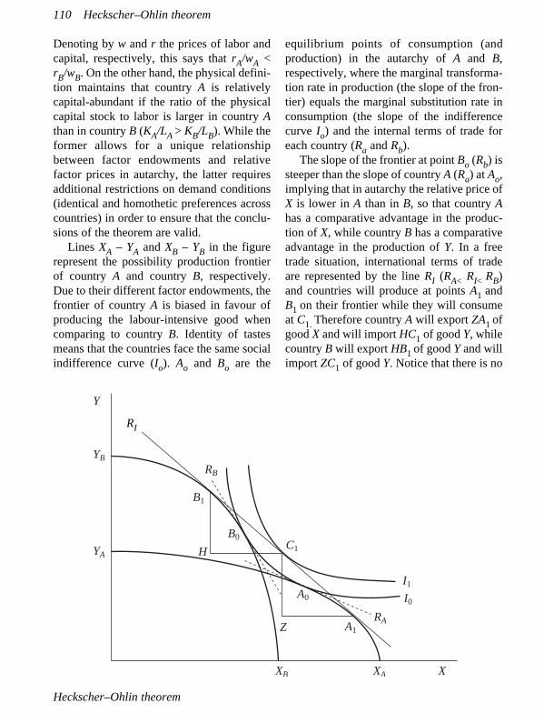
Denoting by w and r the prices of labor andcapital, respectively, this says that rA/wA <rB/wB. On the other hand, the physical defini-tion maintains that country A is relativelycapital-abundant if the ratio of the physicalcapital stock to labor is larger in country Athan in country B (KA/LA > KB/LB). While theformer allows for a unique relationshipbetween factor endowments and relativefactor prices in autarchy, the latter requiresadditional restrictions on demand conditions(identical and homothetic preferences acrosscountries) in order to ensure that the conclu-sions of the theorem are valid.

Lines XA – YA and XB – YB in the figurerepresent the possibility production frontierof country A and country B, respectively.Due to their different factor endowments, thefrontier of country A is biased in favour ofproducing the labour-intensive good whencomparing to country B. Identity of tastesmeans that the countries face the same socialindifference curve (Io). Ao and Bo are the

equilibrium points of consumption (andproduction) in the autarchy of A and B,respectively, where the marginal transforma-tion rate in production (the slope of the fron-tier) equals the marginal substitution rate inconsumption (the slope of the indifferencecurve Io) and the internal terms of trade foreach country (Ra and Rb).

The slope of the frontier at point Bo (Rb) issteeper than the slope of country A (Ra) at Ao,implying that in autarchy the relative price ofX is lower in A than in B, so that country Ahas a comparative advantage in the produc-tion of X, while country B has a comparativeadvantage in the production of Y. In a freetrade situation, international terms of tradeare represented by the line RI (RA< RI< RB)and countries will produce at points A1 andB1 on their frontier while they will consumeat C1. Therefore country A will export ZA1 ofgood X and will import HC1 of good Y, whilecountry B will export HB1 of good Y and willimport ZC1 of good Y. Notice that there is no

110 Heckscher–Ohlin theorem

Heckscher–Ohlin theorem

B0

H

RB

B1

C1

A0

A1

I1

I0

RAZ

XB XA X

YA

YB

Y

R1RI

world excess in demand or supply in any ofthe goods (as expected from the perfectcompetition assumption), so that RI repre-sents the equilibrium terms of trade.

Therefore international trade expandsuntil relative commodity prices are equalizedacross countries, allowing, under previousassumptions, the equalization of relative andabsolute factor prices. This result, thatfollows directly from Heckscher–Ohlin, isknown as the ‘factor price equalization the-orem’ or the Heckscher–Ohlin–Samuelsontheorem and implies that free internationaltrade in goods is a perfect substitute for theinternational mobility of factors.

TERESA HERRERO

BibliographyBhagwati, Jagdish, A. Panagariya, and T.N. Srinivasan,

(1998), Lectures on International Trade, Cam-bridge, MA: MIT Press, pp. 50–79.

Heckscher, Eli (1919), ‘The effect of foreign trade onthe distribution of income’, Economisk Tidskrift, 21,1–32. Reprinted in H.S. Ellis and L.A. Metzler (eds)(1949), Readings in the Theory of InternationalTrade, Philadelphia: Blakiston.

Ohlin, Bertil (1933), Interregional and InternationalTrade, Cambridge, MA: Harvard University Press,esp. pp. 27–45.

Samuelson, Paul (1948), ‘International trade and theequalization of factor prices’, Economic Journal, 58,163–84.

Herfindahl–Hirschman indexThe Herfindhal–Hirschman index (HHI) isdefined as the sum of the squares of themarket shares (expressed in percentages) ofeach individual firm. As such, it can rangefrom 0 to 10 000, from markets with a verylarge number of small firms to those with asingle monopolistic producer. Decreases inHHI value generally indicate a loss of pricingpower and an increase in competition,whereas increases imply the opposite. Theindex is commonly used as a measure ofindustry concentration. For instance, it hasbeen shown theoretically that collusionamong firms can be more easily enforced in

an industry with high HHI. In addition, manyresearchers have proposed this index as agood indicator of the price–cost margin and,thus, social welfare.

Worldwide, antitrust commissions evalu-ate mergers according to their anticipatedeffects upon competition. In the UnitedStates, a merger that leaves the market withan HHI value below 1000 should not beopposed, while a merger that leaves themarket with an HHI value that is greater than1800 should always be opposed. If themerger leaves the market with an HHI valuebetween 1000 and 1800, it should only beopposed if it causes HHI to increase by morethan 100 points.

The index was first introduced by AlbertO. Hirschman (b.1915) as a measure ofconcentration of a country’s trade incommodities. Orris C. Herfindahl (b.1918)proposed the same index in 1950 for measur-ing concentration in the steel industry andacknowledged Hirschman’s work in a foot-note. Nevertheless, when the index is used, itis now usually referred to as the Herfindhalindex. ‘Well, it’s a cruel world,’ wasHirschman’s response to this.

ALBERTO LAFUENTE

BibliographyHerfindahl, O.C. (1950), ‘Concentration in the US steel

industry’, unpublished doctoral dissertation,Columbia University.

Hirschman, A.O. (1945), National Power and theStructure of Foreign Trade, Berkeley, CA:University of California Bureau of Business andEconomic Research.

Hirschman, A.O. (1964), ‘The paternity of an index’,American Economic Review, 54, 761.

Hermann–Schmoller definitionNet income was defined by Hermann (1832,p. 112) and in the same way by Schmoller(1904, pp. 177–8) thus: ‘The flow of rentproduced by a capital without itself suffer-ing any diminution in exchange value’(Schumpeter, pp. 503, 628). Friedrich B.W.

Hermann–Schmoller definition 111

von Hermann (1795–1868) was a Bavariancivil servant, political economist and professorat the University of Munich, where he studiedincome and consumption and publishedStaatswirtschaftliche Untersuchungen in1832. Gustav von Schmoller (1838–1917),professor at Halle, Strassburg and Berlin, wasthe leader of the German ‘younger’ HistoricalSchool who engaged in a methodologicaldispute or methodenstreit with Carl Menger,the founder of the Austrian School, and upheldan inductivist approach in many books andessays.

According to Hermann, with respect tocapital goods, ‘rent can be conceived as agood in itself . . . and may acquire anexchange value of its own . . . retaining theexchange value of capital’ (1832, pp. 56–7).Schmoller shared this view: capital shouldnot be identified with accumulated wealthbut with patrimony/property. For bothauthors the first meaning of capital is netincome.

REYES CALDERÓN CUADRADO

BibliographyHermann, F. von (1832), Staatswirtschaftliche

Untersuchungen über Bermogen, Wirtschaft,Productivitat der Arbeiten, Kapital, Preis, Gewinn,Einkommen und Berbrauch, reprinted (1987),Frankfurt: Wirtschaft und Finanzen.

Schmoller, G. von (1904), Grundriss der AllgemeinenVolkswirtschaftslehre, vol. II, reprinted (1989),Düsseldorf: Wirtschaft und Finanzen.

Schumpeter, J.A. (1954), History of Economic Analysis,New York: Oxford University Press.

Hessian matrix and determinantThe Hessian matrix H(f (x→0)) of a smooth realfunction f(x→), x→∈ Rn, is the square matrixwith (i, j) entry given by ∂2f (x→0)/∂xj∂xi. Itwas introduced by the German mathema-tician L.O. Hesse (1811–74) as a tool inproblems of analytic geometry.

If f belongs to the class C2 (that is, all itssecond order derivatives are continuous) inan open neighbourhood U of x→0, then the

Hessian H(f(x→0)) is a symmetric matrix. If Uis a convex domain and H(f(x→)) is positivesemidefinite (definite) for all x→∈ U, then f is aconvex (strictly convex respectively) func-tion on U. If H(f(x→)) is negative semidefinite(definite), then f is concave (strictly concave)on U.

If x→0 is a critical point (∇ f (x→0) = 0) andH(f(x→0)) is positive (negative) definite, thenx→0 is a local minimum (maximum). Thisresult may be generalized to obtain sufficientsecond-order conditions in constrained opti-mization problems if we replace the objec-tive function f with the Lagrangian L(x→, l

→) =

f(x→) – l→

¡ (g→(x→) – b→

), where g→(x→) = b→

are theconstraints of the problem. The Hessianmatrix of the Lagrangian is called the‘bordered Hessian matrix’, and it plays ananalogous role to the ordinary Hessianmatrix in non-constrained problems.

The determinant of the Hessian matrixoften arises in problems of economic analy-sis. For instance, the first-order necessaryconditions of consumption and productionoptimization problems take the form ∇ f (x→0,p→0) = 0

→where p→0 is some parameter vector,

usually the price vector of consumptiongoods or production factors. In order toobtain from this system of (non-linear) equa-tions the demand functions, which give theoptimal quantities of goods or productionfactors to be consumed as a function of theparameter vector in a neighbourhood of (x→0,p→0), we must ensure that the Jacobian of ∇ f (x→, p→), which is the Hessian determinant,does not vanish at (x→0, p→0). This is, there-fore, a necessary condition for the existenceof demand functions in these problems. Thepositive or negative definiteness of theHessian matrix in (x→0, p→0) provides suffi-cient second-order conditions which ensurethat the demand functions obtained in thisway indeed give (local) optimal consump-tions.

MANUEL MORÁN

112 Hessian matrix and determinant

BibliographySimons, C.P. and L. Blume (1994), Mathematics for

Economists, New York and London: W.W. Norton.

Hicks compensation criterionThe so-called ‘Hicks compensation criterion’is nothing but the inverse factor of the binaryrelation proposed originally by Kaldor.

LUÍS A. PUCH

BibliographyHicks, J.R. (1939), ‘The foundations of welfare econom-

ics’, Economic Journal, 49, 696–712.

See also: Chipman–Moore–Samuelson compensationcriterion, Kaldor compensation criterion, Scitovski’scompensation criterion.

Hicks composite commoditiesAlmost any study in economics, in order tomake it tractable, implicitly or explicitly,involves certain doses of aggregation of thegoods considered (think of food, labour,capital and so on). John R. Hicks (1904–89,Nobel Prize 1972) provided in 1936 thefirst set of conditions under which onecould consider different goods as a uniquecomposite good (normally called thenumeraire). Citing Hicks, ‘if the prices of agroup of goods change in the same propor-tion, that group of goods behaves just as ifit were a single commodity’. In otherwords, what is needed is that the relativeprices in this set of commodities remainunchanged.

Formally, consider a consumer withwealth w and a utility function u(x, y) overtwo sets of commodities x and y, with corre-sponding prices p and q. Assume that theprices for good y always vary in proportionto one another, so that q = ay. Then, for anyz > 0, we can define

v(x, z) = MaxU(x, y)y

s.t.: ay ≤ z

and reconsider the original consumptionproblem as defined over the goods x and thesingle composite commodity z with corre-sponding prices p and a, and with the util-ity function v(x, z) (which inherits all thewell-behaved properties of the originalone).

There are two essential reasons for theimportance of this result. First, as alreadysaid, it facilitates the aggregate study ofbroad categories by lumping together similargoods (think, for instance, of the consump-tion–leisure decision, or the intertemporalconsumption problem). Second, it alsoprovides solid ground for the justification ofpartial equilibrium analysis. If we are inter-ested in the study of a single market thatconstitutes a small portion of the overalleconomy, we can consider the rest of goods’prices as fixed, and therefore treat the expen-diture on these other goods as a singlecomposite commodity.

GUILLERMO CARUANA

BibliographyHicks, J.R. (1936), Value and Capital, Oxford

University Press.

Hicks’s technical progressTechnical progress is one of the basic ingre-dients, along with the productive inputs, ofany aggregate production function. From aformal perspective and using just two inputs(labour, L, and capital, K) for the sake ofsimplicity, a general specification of theproduction function would be

Yt = F(At, Lt, Kt),

where Y is total output, F is a homogeneousfunction of degree g and A the state of technology. Thus technological progress(changes in the level of technology) can beunderstood as the gains in efficiency accru-ing to the productive factors as knowledge

Hicks’s technical progress 113

and experience accumulate. From an empiri-cal point of view, technological progress isusually calculated residually as that part ofoutput growth which is not explained by thesimple accumulation of the productive inputs;log-differentiating the previous expression,technological progress is formally obtained asfollows

FLLt FKKtDat = Dyt – —— Dlt – —— Dkt

Yt Yt

where lower-case variables are the logs ofthe corresponding upper-case variables, D isthe first differences operator and Fx is themarginal factor productivity.

There are a number of ways in which thistechnological progress can be characterized,according to its impact on the intensity withwhich the productive inputs are used. Themain property of the one named after John R.Hicks (1904–89, Nobel Prize 1972) asHicks-neutral technological progress is that itdoes not alter any of the possible pairs ofmarginal productivity ratios among thedifferent inputs that are included in theproduction function. This means that theimprovement in efficiency resulting fromtechnological progress is transmitted equallyto all the productive factors. From a formalperspective, Hicks-neutral technologicalprogress can be represented by the followingproduction function:

Yt = AtF(Lt, Kt).

In such a case, the marginal productivityof labour would be AtFL(Lt, Kt), and that ofcapital AtFK(Lt, Kt). As can be seen, the ratioof these two expressions does not depend onA, the technology, implying that technologi-cal progress itself does not affect the relativedemand for productive inputs.

ANGEL ESTRADA

BibliographyHicks, J.R. (1932), The Theory of Wages, London:

MacMillan.

See also: Harrod’s technical progress.

Hicksian demandJohn R. Hicks (1904–89) was one of theleading figures in the development ofeconomic theory. He made seminal contribu-tions to several branches of economics,including the theory of wages, value theory,welfare analysis, monetary economics andgrowth theory. He shared the Nobel Prize inEconomics with K.J. Arrow in 1972. Hispaper with R.G.D. Allen (1934), showed thatthe main results of consumer theory can beobtained from utility maximization andintroduced the decomposition of demandinto substitution and income effects. In thispaper, he defined what is known as ‘Hicksiandemand’, which is obtained by changing thewealth as the level of price changes, keepingan index of utility constant.

Formally, Hicksian demand is the out-come of the expenditure minimization prob-lem that computes the minimum level ofwealth required to obtain a fixed level of util-ity u0, taking the price vector p ∈ Rn

++ asgiven. This problem can be written asfollows:

Minx≥0 pxs.t. u(x) ≥ u0.

Under the usual assumption of monotonepreferences, the solution to this problemexists. The optimal consumption bundle isknown as the (unobservable) Hicksiandemand, which is usually denoted by h (p, u)∈ Rn

+. As prices change, h(p, u) indicates thedemand that would arise if consumers’wealth was adjusted to keep their level of utility constant. This contrasts withMarshallian demand, which keeps wealthfixed but allows utility to change. Hence

114 Hicksian demand

wealth effects are absent and h(p, u)measures only the cross–substitution effectsof price changes. This explains why Hicksiandemand is also known as ‘compensateddemand’.

The expenditure minimization problemthat yields the Hicksian demand is the dual ofthe utility maximization problem. If the usualassumptions about preferences hold, u(x) is acontinuous and monotonic utility functionrepresenting these preferences and p >> 0,then the solutions to both problems coincide.In particular, if x* is optimal in the utilitymaximization problem when wealth is w*, x*

is also the solution to the expenditure mini-mization problem when u0 = u(x*) and thelevel of expenditure in equilibrium is w*.Therefore, under the above assumptions,Marshallian and Hicksian demands are ident-ical.

XAVIER TORRES

BibliographyHicks, J.R. and R.G.D. Allen (1934), ‘A reconsideration

of the theory of value’, Parts I and II, Economica,N.S., Feb. I (1), 52–76; May II (2), 196–219.

Mas-Colell, A., M.D. Whinston and J.R. Green (1995),Microeconomic Theory, Oxford University Press.

See also: Marshallian demand, Slutsky equation.

Hicksian perfect stabilityContrary to Marshall’s ‘applied economics’interest in market stability, the motivationbehind Sir John R. Hicks’s (1904–89, NobelPrize 1972) analysis of this issue was a theor-etical one. In the opening paragraph ofChapter V of Value and Capital, one canread

The laws of change of the price-system [. . .]have to be derived from stability conditions.We first examine what conditions are neces-sary in order that a given equilibrium systemshould be stable; then we make an assumptionof regularity, that positions in the neighbour-hood of the equilibrium position will be stablealso; and thence we deduce rules about the

way in which the price-system will react tochanges in tastes and resources’ (Hicks, 1939,p. 62).

In other words, if stability is taken forgranted we can do comparative static analy-ses for changes in the relevant parameters.

Hicks’s concept of ‘perfect stability’ is ageneralization of the Walrasian stabilitycondition (through tâtonnement) in whichprice changes are governed by excessdemands. This issue had been successfullysettled by Walras but only for the case of twocommodities in a pure exchange economy.According to Hicks, a price system isperfectly stable if the rise (fall) of the price ofany good above (below) its equilibrium levelgenerates an excess supply (demand) of thatgood, regardless of whether or not the pricesof other commodities are fixed or adjusted toensure equilibrium in their respectivemarkets.

The original proof (Hicks, 1939, math-ematical appendix to Chapter V, pp. 315–19)in the case of n goods and N consumersconsists of the determination of mathemat-ical conditions ensuring the negative sign ofthe derivatives of every good’s excessdemand function with respect to its ownprice when (i) all other prices remainconstant, (ii) another price adjusts so as tomaintain equilibrium in each market but allother prices remain unchanged, (iii) anyother two prices adjust so as to maintainequilibrium in both of their respectivemarkets but all other prices remainunchanged . . . until all prices are adjustedexcept for the price of the numeraire goodwhich is always unity. The well-knownnecessary condition is that the value of thedeterminants of the principal minors of theJacobian matrix of the excess demand func-tions must be alternatively negative and posi-tive. The only possible cause of instability ina pure exchange economy is the asymmetryof consumer income effects.

Hicksian perfect stability 115

One obvious limitation of Hicksian stabil-ity, besides its local nature, is that it is ashort-term (‘within the week’ in Hicks’s ownwords) analysis. But the most importantweakness, as Samuelson (1947) pointed out,is its lack of a specified dynamic adjustmentprocess for the economy as a whole. TheHicksian condition is neither necessary norsufficient for dynamic stability. Never-theless, the usefulness of the Hicksianconcept in comparative static has generated alot of research on the relationship betweenthe conditions for perfect stability and fortrue dynamic stability. It was shown that theyoften coincide (Metzler, 1945). They do so,for example, particularly when the Jacobianmatrix of excess demand is symmetric orquasi-negative definite and also when allgoods are gross substitutes.

JULIO SEGURA

BibliographyHicks, J.R. (1939), Value and Capital, Oxford: Oxford

University Press (2nd edn 1946).Metzler, L. (1945), ‘Stability of multiple markets: the

Hicks conditions’, Econometrica, 13, 277–92.Samuelson, P.A. (1947), Foundations of Economic

Analysis, Cambridge, MA: Harvard UniversityPress.

See also: Lange–Lerner mechanism, Lyapunov stabil-ity, Marshall’s stability, Walras’s auctioneer andtâtonnement.

Hicks–Hansen modelThe Hicks–Hansen or IS–LM model, devel-oped by Sir John R. Hicks (1904–89, NobelPrize 1972) and Alvin H. Hansen (1887–1975), was the leading framework of macro-economic analysis from the 1940s to themid-1970s.

Hicks introduced the IS–LM model in his1937 article as a device for clarifying therelationship between classical theory and TheGeneral Theory of Employment Interest andMoney (1936) of John Maynard Keynes.Hicks saw as Keynes’s main contribution the

joint determination of income and the inter-est rate in goods and financial markets. Hisearly mathematical formalization of animportant but very difficult book providedthe fulcrum for the development ofKeynesian theory, while spurring endlessdebates on whether it captured Keynes’sideas adequately. Hansen (1949, 1953)extended the model by adding, among otherthings, taxes and government spending.

The simplest IS–LM model has threeblocks. In the goods market, aggregatedemand is given by the sum of consumptionas a function of disposable income, invest-ment as a function of income and the interestrate, and government spending. In equilib-rium, aggregate demand equals aggregatesupply and so investment equals saving,yielding the IS curve. In money market equi-librium, money demand, which depends onincome and the interest rate, equals moneysupply, giving rise to the LM curve (liquiditypreference – as Keynes called moneydemand – equals money). In the third blockemployment is determined by output throughan aggregate production function, withunemployment appearing if downward rigid-ity of the nominal wage is assumed. Jointequilibrium in the output–interest rate spaceappears in the figure below. The analysis ofmonetary and fiscal policies is straightfor-ward: lower taxes and higher governmentspending shift the IS curve out (having amultiplier effect) and higher money supplyshifts the LM curve out.

The IS–LM model represents a static,short-run equilibrium. Not only the capitalstock but also wages and prices are fixed,and expectations (crucial in Keynesiantheory as ‘animal spirits’) play virtually norole. Given that the IS captures a flow equi-librium and the LM a stock equilibrium, thejoint time frame is unclear. There is noeconomic foundation for either aggregatedemand components or money demand,and output is demand-determined. These

116 Hicks–Hansen model

limitations stimulated the rise of modernmacroeconomics.

In the 1950s, Franco Modigliani andMilton Friedman developed theories ofconsumption, and James Tobin developedtheories of investment and money demand.The lack of dynamics was tackled by addinga supply block constituted by the Phillipscurve, an empirical relationship apparentlyimplying a reliable trade-off between theunemployment rate and price inflation. In the1960s, the IS–LM was enlarged by RobertMundell and Marcus Fleming to encompassthe open economy.

The extended IS–LM, called the ‘neoclas-sical synthesis’ or, later, the ‘Aggregatesupply–aggregate demand model’, gave riseto large macroeconometric models, such asthe MPS model, led by Franco Modigliani inthe 1960s. It was seen and used as a reliabletool for forecasting and for conducting policyin fine-tuning the economy, this in spite ofcontinuing criticism from the monetarists,led by Milton Friedman, who argued that

there was no long-run inflation–unemploy-ment trade-off and that monetary policyrather than fiscal policy had the strongestimpact on output, but also that, since it couldbe destabilizing, it should stick to a constantmoney growth rule.

The IS–LM model is still the backbone ofmany introductory macroeconomics text-books and the predictions of its extendedversion are consistent with many empiricalfacts present in market economies. However,it is now largely absent from macroeconomicresearch. Its demise was brought about bothby its inability to account for the simul-taneous high inflation and unemploymentrates experienced in the late 1970s, owing to its non-modelling of the supply side, andby its forecasting failures, which lent supportto the Lucas critique, which stated thatmacroeconometric models which estimateeconomic relationships based on past poli-cies without modelling expectations as ratio-nal are not reliable for forecasting under newpolicies. Current macroeconomic research is

Hicks–Hansen model 117

Output

Interestrate

LM

IS

Hicks–Hansen, or IS–LM, model

IS

conducted using dynamic general equilib-rium models with microeconomic founda-tions which integrate the analyses of businesscycles and long-term growth. However, theidea that wage and price rigidities helpexplain why money affects output and thatthey can have important effects on businesscycle fluctuations, a foundation of theIS–LM model, survives in so-called ‘newKeynesian’ macroeconomics.

SAMUEL BENTOLILA

BibliographyHansen, A.H. (1949), Monetary Theory and Fiscal

Policy, New York: McGraw-Hill.Hansen, A.H. (1953), A Guide to Keynes, New York:

McGraw-Hill.Hicks, J.R. (1937), ‘Mr. Keynes and the “Classics”; a

suggested interpretation’, Econometrica, 5 (2),147–59.

Keynes, J.M. (1936), The General Theory ofEmployment Interest and Money, New York:Macmillan.

See also: Friedman’s rule for monetary policy,Keynes’s demand for money, Lucas critique,Mundell–Fleming model, Phillips curve.

Hodrick–Prescott decompositionThe evolution of the economic activity ofindustrialized countries indicates that aggre-gate production grows, oscillating around atrend. One of the problems that attracted mostattention in the history of economics is how todecompose the aggregate production into thetwo basic components: the trend and the cycle(business cycle). Until very recently, differenteconomic models were used to explain theevolution of each component. However,modern real business cycle theory tries toexplain both components with the same typeof models (stochastic growth models, forexample). In order to evaluate or calibrate theeconomic implications of those models it isnecessary to define each component.

The Hodrick and Prescott (Edward C.Prescott, b. 1940, Nobel Prize 2004) (1980)paper, published in 1997, represents an inter-

esting approach, known as the Hodrick–Prescott (HP) filter. The filter works asfollows: first, the trend component is gener-ated for a given value of l and, second, thecycle is obtained as the difference between theactual value and the trend. This parameter l isfixed exogenously as a function of the period-icity of the data of each country (quarterly,annually, and so on). For a value of l = 0 theeconomic series is a pure stochastic trend withno cycle and for large values of l (say l > 100000) the series fluctuates (cyclically) around alinear deterministic trend. In the US economythe values most commonly used are l = 400for annual data and l = 1.600 for quarterlydata. With those values the cyclical compo-nent obtained eliminates certain low frequen-cies components, those that generate cycles ofmore than eight years’ duration.

ALVARO ESCRIBANO

BibliographyHodrick R. and E.C. Prescott (1997), ‘Postwar U.S.

business cycles: a descriptive empirical investiga-tion’, Journal of Money, Credit and Banking, 29(1), 1–16; discussion paper 451, NorthwesternUniversity (1980).

Hotelling’s model of spatial competitionHarold Hotelling (1929) formulated a two-stage model of spatial competition in whichtwo sellers first simultaneously choose loca-tions in the unit interval, and then simul-taneously choose prices. Sellers offer ahomogeneous good produced at zero cost.Consumers are evenly distributed along theinterval, and each of them buys one unit ofthe good from the seller for which price plustravel cost is lowest. Another interpretationof this model is that consumers have differ-ent tastes, with the line representing its distri-bution, and they face a utility loss from notconsuming their preferred commodity.

In Hotelling’s original formulation, travelcosts are proportional to distance, and for thissetting he claimed that both sellers will tend to

118 Hodrick–Prescott decomposition

locate at the centre of the interval (principle ofminimum differentiation). This statement hasbeen proved to be invalid as, with linear trans-port costs, no price equilibrium exists whensellers are not far enough away from eachother. Minimum differentiation may not hold.Fixing the location of one seller, the other hasincentives to move closer so as to capture moreconsumers. But since price is chosen afterlocations are set, sellers that are close willcompete aggressively, having the incentive tolocate apart so as to weaken this competition.

To circumvent the problem of non-exist-ence of equilibrium, Hotelling’s model hasbeen thoroughly worked through in terms ofaltering the basic assumptions in the model.In particular, D’Aspremont et al. (1979) haveshown the existence of an equilibrium forany location of the two firms when transportcosts are quadratic. For this version, there isa tendency for both sellers to maximize theirdifferentiation (principle of maximum differ-entiation).

Hotelling’s (1929) model has been shownto provide an appealing framework toaddress the nature of equilibrium in charac-teristic space and in geographic space, and ithas also played an important role in politicalscience to address parties’ competition.

M. ANGELES DE FRUTOS

BibliographyD’Aspremont, C., J.J. Gabszewicz and J.F. Thisse

(1979), ‘On Hotelling’s “Stability in Competition” ’,Econometrica, 47, 1145–50.

Hotelling, H. (1929), ‘Stability in competition’,Economic Journal, 39, 41–57.

Hotelling’s T2 statisticThe statistic known as Hotelling’s T2 wasfirst introduced by Hotelling (1931) in thecontext of comparing the means of twosamples from a multivariate distribution. Weare going to present T2 in the one sampleproblem in order to better understand thisimportant statistic.

Let us start by recalling the univariatetheory for testing the null hypothesis H0; m =m0 against H1; m ≠ m0. If x1, x2, . . ., xn is arandom sample from a normal populationN(m, s), the test statistics is

(x– – m0)t = ———,

S——

��n

with x– and S being the sample mean and thesample standard deviation.

Under the null hypothesis, t has a Studentt distribution with v = n – 1 degrees of free-dom. One rejects H0 when | t | exceeds aspecified percentage point of the t-distribu-tion or, equivalently, when the p value corre-sponding to t is small enough. Rejecting H0when | t | is large is equivalent to rejecting H0when its square,

(x– – m0)2

t2 = ———— = n(x– – m0) (S2)–1 (x– – m0),S2

——n

is large.In the context of one sample from a multi-

variate population, the natural generalizationof this squared distance is Hotelling’s T2

statistic:

T2 = n(x– – m0)1 (S—)–1 (x– – m0), (1)

where

1 n

x– = — ∑xjn j=1

is a p-dimensional column vector of samplemeans of a sample of size n (n > p) drawnfrom a multivariate normal population ofdimension p. Np(m; ∑) with mean m andcovariance matrix ∑.

Hotelling’s T2 statistic 119

S is the sample covariance matrix esti-mated with n – 1 degrees of freedom

1 n

S = —— ∑(xj – x–)(xj – x–)�).n – 1 j=1

A vector is denoted u, a matrix A and A–1 andA� are the inverse and the transpose of A.

The statistic (1) is used for testing the nullhypothesis H0: m = m0 versus H1: m = m1 ≠ m0.If the null hypothesis is true, the distributionof

(n – p)——— T2

p(n – 1)

is the F distribution with degrees of freedomp and n – p.

Departures of m– from m–0 can only increasethe mean of T2 and the decision rule for a testof significance level a is

p(n – 1)reject H0: m = m0 if T2 > ——— Fa,p,n–p.

n – p

ALBERT PRAT

BibliographyHotelling H. (1931), ‘The generalization of Student’s

ratio’, Annals of Mathematical Statistics, 2, 360–78.

Hotelling’s theoremNamed after Harold Hotelling (1895–1973),and containing important implications forconsumers’ duality, the theorem establishesthat, if the expenditure functions can bedifferenced, the Hicksian demand functions(in which the consumer’s rent is compen-sated to achieve a certain utility level) are thepartial derivatives of the expenditure func-tions with respect to the correspondingprices.

If h(p, U) is the Hicksian demand vectorthat solves the consumer’s dual optimizationproblem, the expenditure function, e(p, U) is

defined as the minimum cost needed toobtain a fixed utility level with given prices:

e(p, U) = p · h(p, U) = ∑pihi(p, U) ∀ i = 1 . . . n.i

Differencing the expenditure function byHotelling’s theorem we have

∂e(p, U)———— = hi(p, U) ∀ i = 1 . . . n.

∂pi

The theorem has implications on con-sumer’s duality. It allows us to deducesome of the Hicksians demand propertiesfrom the expenditure function properties. Ifthis function is first degree homogeneous inthe price vector (p), Hicksian demands arezero degree homogeneous, that is to say,demands do not vary if all the goods’ priceschange in the same proportion. If theexpenditure function is concave in the pricevector (p), this indicates the decreasing of agood’s Hicksian demand with respect to itsown price, and establishes the negative signof the substitution effect of this price’svariation:

∂2e(p, U) ∂hi(p, U)———— = ———— < 0 ∀ i = 1 . . . n.

∂p2i ∂pi

On the other hand, Hotelling’s theorem,together with the basic duality that postulatesthe identity of primal and dual solutions ifthey exist, solves the integrability problem.So, whenever the expenditure function andits properties and the Hicksian demandsverify the symmetry condition of the crosssubstitution effects of a price change,

∂hi(p, U) ∂hj(p, U)———— = ———— ∀ i ≠ j,

∂pj ∂pi

it is possible to deduce the only utility func-tion from which they derive, that underlies

120 Hotelling’s theorem

the consumer’s optimization problem andsatisfies the axioms of consumer’s choice.

MA COVADONGA DE LA IGLESIA VILLASOL

BibliographyHotelling H. (1932), ‘Edgworth’s taxation paradox and

the nature of demand and supply functions’, Journalof Political Economy, 40 (5), 578–616.

See also: Hicksian demand, Slutsky equation.

Hume’s forkAll knowledge is analytic or empirical.Scottish philosopher David Hume (1711–76)distinguished between matters of fact, thatcould only be proved empirically, and rela-tions between ideas, that could only beproved logically. The distinction, known asHume’s fork, rules out any knowledge notrooted in ideas or impressions, and has to dowith philosophical discussions about thescientific reliability of induction–synthesisversus deduction–analysis. It is thus stated inthe last paragraph of his Enquiry concerningHuman Understanding:

When we run over libraries, persuaded of theseprinciples, what havoc must we make? If wetake in our hand any volume – of divinity orschool metaphysics, for instance – let us ask,Does it contain any abstract reasoningconcerning quantity or number? No. Does itcontain any experimental reasoning concern-ing matter of fact and existence? No. Commitit then to the flames: For it can contain nothingbut sophistry and illusion.

D.N. McCloskey mentioned Hume’s fork asthe golden rule of methodological modern-ism in economics, and strongly criticized itsvalidity.

CARLOS RODRÍGUEZ BRAUN

BibliographyHume, David (1748), An Enquiry Concerning Human

Understanding, first published under this title in1758; reprinted in T.H. Green and T.H. Grose (eds)

(1882), David Hume. Philosophical Works, vol. 4, p.135.

McCloskey, D.N. (1986), The Rhetoric of Economics,Brighton: Wheatsheaf Books, pp. 8, 16.

Hume’s lawThis refers to the automatic adjustment of acompetitive market balance of internationalpayments based on specie standard.Although the basic components had alreadybeen stated by notable predecessors, asThomas Mun (1630), Isaac Gervaise (1720)or Richard Cantillon (1734) tried to system-atize them, the influential exposition of themechanism was presented by the Scottishphilosopher and historian David Hume(1711–76) in the essay ‘Of the balance oftrade’, published in 1752. The law wasbroadly accepted and inspired classicaleconomics, as it proved that the mercantilis-tic target of a persistently positive balance oftrade and consequent accumulation of goldwas unsustainable.

Hume’s law is an application of the quan-tity theory of money. Starting from an equi-librium in the balance of trade, in a pure goldstandard an increase in the money stock leadsto a proportionate rise in the price level,absolute and relative to other countries. Asthe domestic goods become less competitive,the country will increase its imports anddecrease its exports, and the gold outflowwill reduce prices until the international pricedifferentials are eliminated.

The conclusion is that money is a ‘veil’that hides the real functioning of theeconomic system. The amount of money in anation is irrelevant, as the price level adjuststo it. Nonetheless, Hume recognized thatspecie flow was indirectly a causal factor thatpromotes economic development as itchanges demand and saving patterns. In theshort run, before it increases all prices,money can promote wealth. For this reason,Adam Smith denied Hume’s argument as, inthe end, it demonstrated that specie waswealth (Smith, 1896, p. 507).

Hume’s law 121

Although it is sometimes referred to as thespecie-flow mechanism, Humes’s law wasspecifically a price–specie–flow mechanism.It has been objected that the mechanismassigns a crucial role to differences betweendomestic and foreign prices, but it wouldwork ‘even if perfect commodity arbitrageprevented any international price differentialfrom emerging’ (Niehans, 1990, p. 55). Butthe model, even as a price mechanism, hasbeen found problematic. For example, theself-correction of the trade balance dependson the demand elasticities of our exports inother countries and of our imports in our owncountry. When, say, the foreign demand elas-ticity of our exports is sufficiently small, therise of prices can increase, instead ofdecreasing, the trade surplus, as the exports’value increases. The consequent specieinflow can result in a cumulative increase inprices and export values. Besides, we canimagine other price self-regulatory mecha-nisms. For instance, when there is a specieinflow, the prices of the internationally

traded goods will not increase to the sameextent as those of the non-internationallytradables, as the decrease in the demand forthem in the countries that are losing specieneutralizes the price increases. Domesticconsumers will prefer the now cheaper inter-national goods, absorbing exportables; andproducers will prefer the now dearer non-internationally tradables, reducing the exportsbalance. This mechanism will continue untilthe trade balance is adjusted.

ESTRELLA TRINCADO

BibliographyHume, David (1752), ‘Of the balance of trade’; reprinted

in E. Rotwein (ed.) (1970), David Hume: Writingson Economics, Madison: University of WisconsinPress.

Niehans, Jürg (1990), A History of Economic Theory.Classic Contributions 1720–1980, Baltimore andLondon: The Johns Hopkins University Press.

Smith, Adam (1896), Lectures on Jurisprudence,reprinted in R.L. Meek, D.D. Raphael and P.G. Stein(eds) (1978), The Glasgow Edition of the Works andCorrespondence of Adam Smith, vol. V, Oxford:Oxford University Press.

122 Hume’s law

Itô’s lemmaIn mathematical models of evolution, weprescribe rules to determine the next positionof a system in terms of its present position. Ifwe know the starting position, we may calcu-late the position of the system at any furthertime T by applying recursively that rule. Ifthe model is a continuous time model, theevolution rule will be a differential equation,and differential calculus, particularly thechain rule, will allow us to resolve in aformula the position at time T.

If we incorporate uncertainty in themodelling by prescribing that the next posi-tion is to be decided by means of a drawingfrom a particular probability distributionthen we have a stochastic differential equa-tion.

The Japanese mathematician Kiyoshi Itôcompleted the construction of a whole theoryof stochastic differential equations based onBrownian motion, almost single-handedly.He was mainly motivated by his desire toprovide a firm basis to the naive modelling offinancial markets that had been proposed byLouis Bachelier at the beginning of the twen-tieth century in his celebrated doctoraldissertation, Théorie de la Spéculation whichmay be considered the origin of mathemat-ical finance.

Itô was born in 1915 in Mie, in the south-ern part of the island of Honshu, the mainisland of Japan, and studied mathematics atthe Imperial University of Tokyo. He workedfrom 1938 to 1943 at the Bureau of Statistics,which he left to start his academic career atthe Imperial University at Nagoya. It wasduring his stay at the Bureau of Statistics thathe established the foundations of stochasticcalculus.

Itô’s lemma is one of the main tools of

stochastic calculus. To explain its meaning,we start with a deterministic rule of evolu-tion, such as dx = a(x)dt, and consider thetransformation, y = f(x).

The chain rule tells us that the evolutionof y will be given by dy = f �(x)a(x)dt.However, in a stochastic context, the rulegoverning the evolution is of the form dx =a(x)dt + b(x)dWt. The term dWt is respon-sible for randomness and represents a draw-ing from a normal distribution with meanzero and variance dt, with the understandingthat successive drawings are independent.The notation W honours Norbert Wiener,who provided the foundations of the mathe-matical theory of Brownian motion, that is,the continuous drawing of independentnormal variables. What is the evolution of y= f(x)? How does it relate to the evolution ofx? Candidly, one may think that it should bedy = f �(x)a(x)dt + f �(x)b(x)dWt. However,Itô’s lemma, so surprising at first sight, tellsus that the evolution of y is given by

1dy = f �(x)a(x)dt + — f �(x)b2(x)dt

2

+ f �(x)b(x)dWt.

The puzzling additional term

1— f �(x)b2(x)dt,2

so characteristic of stochastic calculus,comes from the fact that the size of dWt is,on average and in absolute value, ���dt. Byway of example, let us assume that thevalue or the price of a certain good evolvesaccording to dx = x (rdt + s dWt), where rand s are certain constants. This rule

123

I

prescribes an instantaneous return thatoscillates randomly around a certain valuer.

The (continuous) return R that accumu-lates from time 0 to time T is given by

1R = — ln(x(T)/100).

T

Let us compare what happens in a determin-istic situation, when s = 0, with the generalstochastic situation. If s = 0, we consider thetransformation y = ln(x) and, with the help ofthe chain rule, deduce, as expected, that R =r. But, in general, the same argument, butusing now Itô’s lemma, tells us that therandom variable R is

s2 sR = (r – —) + —— Z,

2 ���T

where Z is a drawing from a standard normalvariable. One discovers that, on average,

s2

R = (r – —)2

and not r, as the deterministic case couldhave led us to believe: a lower return, onaverage, than expected at first sight.

In general, Itô’s lemma is importantbecause, when modelling uncertainty, itallows us to focus on the fundamental vari-ables, since the evolution of all other vari-ables which depend upon them can bedirectly deduced by means of the lemma.

JOSÉ L. FERNÁNDEZ

BibliographyItô, K. (1944), ‘Stochastic integral’, Proc. Imp. Acad.

Tokyo, 20, 519–21.

124 Itô’s lemma

Jarque–Bera testThis test consists of applying an asymptoti-cally efficient score test (Lagrange multiplier– LM – test) to derive a test which allows usto verify the normality of observations.

Considering a set of N independent obser-vations of a random variable vi i = 1, 2, 3 . . .N with mean m = E[vi] and vi = m + ui, andassuming that the probability density func-tion of ui is a member of the Pearson family(this is not a very restrictive assumption,given that a wide range of distributions areencompassed in it), the likelihood for thisdistribution will be given by the expression

df(ui)/dui = (c1 – ui)f(ui)/(c0 – c1ui + c2ui2)

(–∞ < ui < ∞).

The logarithm of the likelihood functionfor N observations is

∞ c1 – uil(m, c0, c1, c2) = – N log[∫exp[∫ —————— dui]dui]–∞ c0 – c1ui + c2ui2

N c1 – u1+ ∑[∫ —————— dui].i=1 c0 – c1ui + c2ui2

The assumption of normality implies test-ing H0: c1 = c2 = 0 and, if the null hypothesisis true, the LM test is given by

(m23/m3

2)2 ((m4/m22) – 3)2

LM = N[———— + ——————] = JB,6 24

where mj = ∑(vj – v–) j/N and v– = ∑vi/N. Theexpression m3

2/m23 is the skewness and

m4/m22 is the kurtosis sample coefficient.

This expression is asymptotically distributedas c2

(2) (chi-squared distribution with twodegrees of freedom) under Ho that the obser-vations are normally distributed.

This test can be applied in the regressionmodel yi = xi�b + ui, in order to test thenormality of regression disturbances u1, u2, . . . uN. For this purpose, ordinary leastsquares residuals are used and the LM test, inthe case of linear models with a constantterm, is obtained with the skewness and thekurtosis of the OLS residuals.

Since, for a normal distribution, the valueof skewness is zero and the kurtosis is 3,when the residuals are normally distributed,the Jarque-Bera statistic has an c2

(2) distribu-tion. If the value of Jarque-Bera is greaterthan the significance point of c2

(2), thenormality assumption is rejected.

AMPARO SANCHO

BibliographyJarque, C.M. and A. Bera (1987), ‘A test for normality

of observations and regression residuals’,International Statistical Review, 55, 163–72.

See also: Lagrange multiplier test.

Johansen’s procedureSoren Johansen has developed the likelihoodanalysis of vector cointegrated autoregres-sive models in a set of publications (1988,1991, 1995 are probably the most cited).

Let yt be a vector of m time series inte-grated of order 1. They are cointegrated ofrank r if there are r < m linear combinationsof them that are stationary. In this case, thedynamics of the time series can be repre-sented by a vector error correction model,

∇ yt = Pyt–1 + G1∇ yt–1 + . . . + Gk∇ yt–k+ FDt + et, t = 1, . . ., T,

where ∇ is the first difference operatorsuch that ∇ yt = yt – yt–1, Dt is a vector of

125

J

deterministic regressors (constant, linearterm, seasonal dummies . . .), et are indepen-dently and identically distributed (iid).Gaussain errors (0, ∑) and P, G1, . . ., Gk arem × m parameter matrices, being P = ab�where a and b are m × r matrices. This modelhas gained popularity because it can capturethe short-run dynamic properties as well asthe long-run equilibrium behaviour of manyseries.

Johansen’s procedure determines thecointegration rank r of the previous model bytesting the number of zero canonical correla-tions between ∇ yt and yt–1, once you havecorrected for autocorrelation. Let li be the ithlargest eigenvalue of the matrix

M = S–iii

SijS–1jj Sji,

where Sij = T–1∑RitR�jt, i, j = 0, 1 and R0t andR1t are the residuals of the least squaresregression of ∇ yt and yt–1 over k lags of ∇ ytand Dt. The test statistic for r versus m coin-tegration relations is

m

l(r | m) = –T∑log(1 – li).i=r+1

The distribution of the test is non-standardowing to the non-stationarity of the vector oftime series and the percentiles of the distri-bution have been tabulated by simulation.

PILAR PONCELA

BibliographyJohansen, S. (1988), ‘Statistical analysis of cointegra-

tion vectors’, Journal of Economic Dynamics andControl, 12, 231–54.

Johansen, S. (1991), ‘Estimation and hypothesis testingof cointegration vectors in Gaussian vector autore-gressive models’, Econometrica, 59, 1551–80.

Jones’s magnification effectThe magnification effect is one of the prop-erties of the Heckscher–Ohlin model. It wasenounced by Ronald W. Jones (1965).

Actually there are two magnificationeffects: one concerning the effects ofchanges in factor endowments on outputsand the other concerning the effects ofchanges in commodity prices on factorprices. In the first case, the magnifi-cation effect is a generalization of theRybczynski theorem and in the second it isa generalization of the Stolper–Samuelsontheorem.

As regards factor endowments, themagnification effect says that, if factorendowments expand at different rates, thecommodity intensive in the use of the fastestgrowing factor expands at a greater rate thaneither factor, and the other commoditygrows (if at all) at a slower rate than eitherfactor.

As regards commodity prices, the magni-fication effect says that, if commodity pricesincrease at different rates, the price of thefactor used more intensively in the produc-tion of the commodity with the fastest risingprice grows at a greater rate than eithercommodity price, and the price of the otherfactor grows (if at all) at a slower rate thaneither commodity price.

JUAN VARELA

BibliographyJones, R.W. (1965), ‘The structure of simple general

equilibrium models’, Journal of Political Economy,73, 557–72.

See also: Heckscher–Ohlin theorem, Rybczynskithorem, Stolper–Samuelson theorem.

Juglar cycleThis is an economic cycle lasting nine or tenyears, covering the period of expansionfollowed by a crisis that leads to a depres-sion. It was discovered by the French econ-omist Clément Juglar (1819–1905), who in1848 abandoned his medical studies, turnedhis attention to economics and demography,and was the first to develop a theory of trade

126 Jones’s magnification effect

crises in the context of economic cycles. Hebelieved that such crises could be predicted,but not avoided; like organic illness, theyappeared to be a condition for the existenceof commercial and industrial societies. Juglarpublished studies on birth, death andmarriage statistics of his native country, andalso on financial variables. His most note-worthy book was Des crises commerciales(1862), where he looked to monetary condi-tions to explain the origin and nature ofcrises. In his view, the increase of domesticand foreign trade at prices inflated by specu-lation was one of the chief causes of demandcrises. Juglar’s work gained acceptance

thanks to the positive appraisals of Mitchelland Schumpeter.

JUAN HERNÁNDEZ ANDREU

BibliographyJuglar, Clément (1862), Des crises commerciales et leur

retour périodique en France, en Angleterre et auxEtats-Unis, Paris: Librairie Guillaumin & Cie;presented in the Académie de Sciences Morales etPolitiques in 1860; 2nd edn 1889; a third edition wastranslated into English by W. Thom.

O’Brien, D.P. (ed.) (1997), The Foundations of BusinessCycle Theory, Cheltenham, UK and Lyme, USA:Edward Elgar, vol. I.

Schumpeter, J.A. (1968), History of Economic Analysis,New York: Oxford University Press, p. 1124.

See also: Kitchen cycle, Kondratieff long waves.

Juglar cycle 127

Kakutani’s fixed point theoremShizuo Kakutani (b.1911), a Japanese math-ematician, was a professor at the universitiesof Osaka (Japan) and Yale (USA). Amongthe areas of mathematics on which he haswritten papers we may mention analysis,topology, measure theory and fixed pointtheorems. Kakutani’s theorem is as follows.

Let f: X → X be an upper semicontinuouscorrespondence from a non-empty, compactand convex set X ⊂ Rn into itself such that,for all x ∈ X, the set f (x) is non-empty andconvex. Then f has a fixed point, that is, thereexists x� ∈ X such that x� ∈ f (x�).

This theorem is used in many economicframeworks for proving existence theorems.We mention some of the most relevant.John Nash proved, in 1950, the existence ofNash equilibria in non-cooperative n-persongames. The existence of a competitive equi-librium in an exchange economy wasproved by Kenneth Arrow and GerardDebreu in 1954. Lionel McKenzie proved,in 1954, the existence of equilibrium in amodel of world trade and other competitivesystems.

GUSTAVO BERGANTIÑOS

BibliographyKakutani, S. (1941), ‘A generalization of Brouwer’s

fixed point theorem’, Duke Mathematical Journal,8, 457–9.

See also: Arrow–Debreu general equilibrium model,Graham’s demand, Nash equilibrium.

Kakwani indexThis is a measure of tax progressivity. Aprogressive tax introduces disproportionalityinto the distribution of the tax burden andinduces a redistributive effect on the distri-

bution of income. We can measure theseeffects along the income scale. Suchmeasures are called indices of local or struc-tural progression: liability progression is theelasticity of the tax liability with respect topre-tax income; residual progression is theelasticity of post-tax income with respect topre-tax income.

But we can also quantify the effects of aprogressive tax, once the income distribu-tion to which it will be applied is known.Progressivity indices (or effective progres-sion indices) summarize the tax functionand pre-tax income distribution in a singlenumber. The Kakwani index is one suchprogressivity index. It measures the dispro-portionality in the distribution of the taxburden, that is, the part of the tax burdenthat is shifted from low to high pre-taxincome recipients. Deviation from propor-tionality is evidenced by the separation ofthe Lorenz curve for pre-tax income, andthe concentration curve for tax liabilities. Ifwe denote C to be the concentration indexof taxes and G the Gini index of the pre-taxincome, the Kakwani index, P, can be writ-ten P = C – G.

A progressive tax implies a positive valueof P. Departure from proportionality isclosely related to the redistributive effect: aprogressive tax also shifts part of the post-taxincome from high to low-income recipients.Kakwani has shown that the index of redis-tributive effect, R, is determined by dispro-portionality and the overall average tax rate,t. Neglecting re-ranking (that is, reversals inthe ranking of incomes in the transition frompre-tax to post-tax),

tR = —— P

1 – t

128

K

Effective progression indices satisfy aconsistency property with local or structuralindices: for every pre-tax income distribu-tion, increases in liability progression implyenhanced deviation from proportionality, andincreases in residual progression implyenhanced redistributive effect.

JULIO LÓPEZ LABORDA

BibliographyKakwani, N.C. (1977), ‘Applications of Lorenz curves

in economic analysis’, Econometrica, 45, 719–27.Kakwani, N.C. (1977), ‘Measurement of tax progressiv-

ity: an international comparison’, Economic Journal,87, 71–80.

See also: Reynolds–Smolensky index, Suits index.

Kalai–Smorodinsky bargaining solutionThis is a solution, axiomatically founded,proposed by E. Kalai and M. Smorodinsky(1975), to the ‘bargaining problem’ as analternative to the Nash bargaining solution.

A two-person bargaining problem issummarized by a pair (S, d), where S ⊂ R2

represents the feasible set that consists of allutility pairs attainable by an agreement, andd∈ R2 is the disagreement point, the utilitypair that results if disagreement prevails. It isassumed that d∈ S, and S is compact, convex,comprehensive and contains some point thatstrictly dominates d. A bargaining solution isa function F that associates with eachbargaining problem a point F(S, d) in itsfeasible set.

Nash initiated the present formalization ofbargaining problems and proposed the mostcelebrated of bargaining solutions, the Nashbargaining solution, providing its axiomaticcharacterization. Claiming that a bargainingsolution must be compatible with axioms of efficiency, symmetry, independence ofaffine transformations and independence ofirrelevant alternatives, he proved that theunique solution compatible with these fouraxioms selects the point maximizing the

product of utility gains from d among allpoints of S dominating d.

The independence of irrelevant alterna-tives is somewhat controversial. Moreover,the Nash bargaining solution lacks monoto-nicity: when the set of feasible agreements isexpanded, while the disagreement point andthe maximal aspiration of one of the playersai(S, d) = max{si | s∈ S and sj ≥ dj} and areunchanged, it is not assured that the otherbargainer receives a better allocation.

On the basis of these observations Kalaiand Smorodinsky claim that, instead of theindependence of irrelevant alternatives, asolution ought to satisfy monotonicity: for all(S, d) and (T, d), S ⊂ T and ai(S, d) = ai(T, d),Fj(S, d) ≤ Fj(T, d).

The Kalai–Somorodinsky solution thatselects the maximal point of S in the segmentconnecting d to the maximal aspirationspoint a(S, d) satisfies monotonicity. It satis-fies efficiency, symmetry and independenceof affine transformations as well; and noother solution is compatible with these fouraxioms.

CLARA PONSATI

BibliographyKalai, E. and M. Smorodinsky (1975), ‘Other solutions

to Nash’s bargaining problem’, Econometrica, 43,513–18.

See also: Nash bargaining solution.

Kaldor compensation criterionThe so-called ‘Kaldor compensation crit-erion’, named after Nicholas Kaldor(1908–86), ranks economic alternative xabove economic alternative y if there exists,in the set of alternatives potentially achiev-able from x, an economic alternative z (notnecessarily distinct from x) which Paretodenominates y.

By including the Pareto criterion as asubrelation, the Kaldor criterion clearly satis-fies the Pareto principle. The strong Pareto

Kaldor compensation criterion 129

principle asserts that a sufficient conditionfor ranking an economic alternative aboveanother is when no one in society strictlyprefers the latter and at least one personprefers the former. Economists like to thinkthat, with this principle, they have at theirdisposal a non-controversial criterion toassess whether or not economic transforma-tions are worth doing. A major problem withthis criterion is that the domain of cases towhich it can be applied is rather narrow.

The motivation behind the Kaldor compen-sation criterion is to overcome this difficulty,without invoking other ethical principles, bysuggesting that the domain of cases to whichthe Pareto principle can be applied should beextended from actual cases to potential orhypothetical ones. It is a natural translation ofthe idea of giving priority to actual considera-tions while resorting to potential considera-tions when actual ones are not conclusive.Those rankings of economic alternatives thatare the result of such an idea are known inwelfare economics as compensation criteria àla Kaldor–Hicks–Scitovsky (KHS).

The KHS criterion serves even today as ajustification for using many tools of appliedwelfare economics such as consumer sur-pluses. It is also commonly used incost–benefit analysis. Of course, almostcertainly, unethical interpersonal compari-sons of utility emerge implicitly when theKHS criterion is applied without any actualcompensation occurring.

The usual argument in favour of the KHScriterion is that it extends (albeit incom-pletely) the power of the Pareto principle at alow cost in terms of ethical defensibility.However, the relevance of hypothetical situ-ations for assessing the social desirability ofactual ones is certainly not a principle that iswell established. Further, the KHS criterioncan lead to contradictory (intransitive) policyrecommendations.

LUÍS A. PUCH

BibliographyKaldor, N. (1939), ‘Welfare propositions in economics

and interpersonal comparisons of utility’, EconomicJournal, 49, 549–52.

See also: Chipman–Moore–Samuelson compensationcriterion, Hicks compensation criterion, Scitovski’scompensation criterion.

Kaldor paradoxThis term refers to the positive correlationobserved between the international competi-tiveness of several countries and their relativeunit labour costs. This paradox was notedfirst by Nicholas Kaldor (1908–86) while hewas looking for the causes of the Britishexports share decline in international marketsafter the 1960s. Economic theory had tradi-tionally predicted that export success dependson a low level of prices. But Kaldor observedthat Britain’s international trade share hadbeen declining together with its relative unitlabour costs, while in other countries (Japan,Germany) export trade shares were increas-ing together with their relative unit labourcosts. That is to say, higher wages, costs andprices were not weakening the competitiveposition of Japan and Germany, but, on thecontrary, were contributing to their growingcompetitiveness.

This apparent contradiction was explainedby the ‘non-price’ factors of competitive-ness: the increase of the relative German andJapanese export prices was accompanied byimprovements on other quality factors thatoffset the negative effect of price increase.The ‘non-price’ factors have proved to becrucial for maintaining and increasing thecompetitiveness of industrial economies withhigh wage levels. This important observationincreased the attention given by economistsand policy makers to R&D and educationalinvestments as the proper ways to assure adeveloped country’s competitiveness in thelong term.

JOSÉ M. ORTIZ-VILLAJOS

130 Kaldor paradox

BibliographyKaldor, N. (1978), ‘The effects of devaluation on trade’,

Further Essays on Economic Policy, London:Duckworth.

Kaldor, N. (1981), ‘The role of increasing returns, tech-nical progress and cumulative causation in thetheory of international trade and economic growth’,Économie Appliquée, 34 (4), 593–617.

Kaldor’s growth lawsIn 1966, Nicholas Kaldor (1908–86) pub-lished a study where he tried to explain the‘causes of the slow rate of economic growthin the United Kingdom’, which was anempirical and comparative analysis based onthree theoretical formulations, known asKaldor’s growth laws. The first law statesthat the rates of economic growth are closelyassociated with the rates of growth of thesecondary sector. According to Kaldor, thisis a characteristic of an economy in transi-tion from ‘immaturity’ to ‘maturity’. Thesecond law, also known as the Kaldor–Verdoorn law, says that the productivitygrowth in the industrial sector is positivelycorrelated to the growth of industrial output.It is an early formulation of the endogenousgrowth theory, based on the idea that out-put increase leads to the development of new methods of production (learning-by-doing), which increases productivity. Thisfosters competitiveness and exports and,thus, economic growth, introducing theeconomy into a virtuous circle of cumulativecausation.

The third law gives a special relevance tothe labour factor: economic growth leads towage increases, so the only way for matureeconomies to maintain or increase theircompetitiveness is by shifting their way ofcompeting from price to quality factors. Thisrequires a structural change, which needs alabour transference from the primary to thesecondary sector.

JOSÉ M. ORTIZ-VILLAJOS

BibliographyKaldor, N. (1966), Causes of the Slow Rate of Economic

Growth of the United Kingdom, Cambridge:Cambridge University Press.

Kaldor, N. (1967), Strategic Factors in EconomicDevelopment, Ithaca: Cornell University; Frank W.Pierce Memorial Lectures, October 1966, Geneva,New York: W.F. Humphrey Press.

Thirlwall, A.P. (1983): ‘A plain man’s guide to Kaldor’sgrowth laws’, Journal of Post Keynesian Economics,5 (3), 345–58.

See also: Verdoorn’s law.

Kaldor–Meade expenditure taxThe idea of an expenditure tax dates back atleast as far as the seventeenth century, in theworks of Thomas Hobbes. Nicholas Kaldor(1908–86) proposed his famous ‘expendituretax’ (1955) that was implemented in Indiaand Sri Lanka, when Kaldor worked as anadvisor to both countries. Most recently, inthe UK, it was considered in 1978 by acommittee headed by the British economistJames Meade (1907–95, Nobel Prize 1977).The Meade Committee issued a lengthyreport of their findings.

An expenditure tax is a direct tax in whichthe tax base is expenditure rather thanincome. Income taxes have sometimes beencriticized on the grounds that they involvethe ‘double taxation of savings’. To theextent that income tax does penalize savings,it can be argued to reduce savings in theeconomy and by doing so to reduce the fundsavailable for investment. An expenditure tax,on the other hand, taxes savings only once, at the point at which they are spent.Expenditure taxation is not the equivalent ofindirect taxes such as value added tax. Aswith other direct taxes, it could be levied atprogressive rates, whereas indirect taxes arealmost inevitably regressive in their effects.Personal allowances could also be built intoan expenditure tax regime as in income tax.

Imposing an expenditure tax would notrequire people to keep a record of every item of expenditure. The usual approach

Kaldor–Meade expenditure tax 131

suggested is to start with a person’s grossincome (income + capital receipts + borrow-ing) and then subtract spending on capitalassets, lending and repayment of debt.Consumption expenditure = income + capitalreceipts + borrowing – lending – repaymentof debt – spending on capital assets.

Expenditure taxation avoids need forvaluation of wealth, but information onearned income and net transactions in regis-tered assets is necessary. Some of the advan-tages of the expenditure tax are theavoidance of double taxation of savings andthe inexistence of distortion of intertemporalconsumption decisions due to taxation ofinterest. But a political cost has to be high-lighted: since savings are not included in thetax base, tax rates on the remaining basemust be higher. Also one of the main prob-lems is the transition from income taxation: itis really important to register assets at theoutset. If assets could escape registration,expenditure from subsequent sale of theseassets would be untaxed. Taxation of entre-preneurial incomes could be a problem aswell, since income from a small businessconsists partly of the proprietor’s earnedincome, and partly return on the proprietor’scapital invested.

NURIA BADENES PLÁ

BibliographyKaldor, N. (1955), An Expenditure Tax, London: Unwin

University Books.Meade Committee (1978), The Structure and Reform of

Direct Taxation, London: Institute for Fiscal Studies(report of a committee chaired by Professor J.E.Meade), London: Allen and Unwin.

Kalman filterThe Kalman filter (KF), named after theHungarian mathematician Rudolf EmilKalman (b.1930), is an algorithm to estimatetrajectories in stochastic dynamic systems,intensively used in fields such as engineer-ing, statistics, physics or economics. Its

origins are the work of Gauss on conditionalexpectations and projections, of Fisher on themaximum likelihood method, and of Wienerand Kolmogorov on minimum mean squarederror (MMSE) estimation theory. The explo-sion in computational methods provided thecatalyst. A standard original reference isKalman (1960), although Bucy should alsobe mentioned.

The KF is an efficient algorithm forMMSE estimation of a state variable vector,which is the output of a dynamic model,when the model and the observations areperturbed by noise. (In econometrics, thenoise perturbing the model is often called‘shock’; that perturbing the measurement,‘error’.) The filter requires the model to beset in state space (SS) format, which consistsof two sets of equations. The first set (thedynamic or transition equation) specifies thedynamics of the state variables. The secondset (the measurement equation) relates thestate variables to the observations.

A standard SS representation (among themany suggested) is the following. Let xtdenote a vector of observations, and zt avector of (in general, unobserved) variablesdescribing the state. The transition andmeasurement equations are

zt+1 = At zt + ht,

xt = Mt zt + et,

where At and Mt and are the transition andmeasurement matrices of the system(assumed non-stochastic), and the vectors htand et represent stochastic noise. Althoughthe filter extends to the continuous time case,the discrete time case will be considered. Letxt = (x1, x2, . . ., xt)� denote the vector ofobservations available at time t (for someperiods observations may be missing). Givenxt, the filter yields the MMSE linear estima-tor z flt of the state vector zt.

Assuming (a) an initial state vector, x0,

132 Kalman filter

distributed N(Ex0, ∑0); (b) variables ht, etdistributed N(0, Qt) and N(0, Rt), respec-tively, and (c) mutually uncorrelated x0, htand et, the estimator zflt is obtained throughthe recursive equations:

zfl0 = E z0,

zflt = At–1 zflt–1 + Gt (xt – At–1 zflt–1) for t = 1, 2, . . .

The matrix Gt is the ‘Kalman gain’,obtained recursively through

∑0|0 = ∑0

∑t|t–1 = At–1 ∑t–1|t–1 A�t–1 + Qt–1

Gt = ∑t|t–1 M�t (Mt∑t|t–1 M�t + Rt)–1

∑t|t = (I – Gt Mt)∑t|t–1 (t = 1, 2, . . .)

and ∑t|t–1 is the covariance of the predictionerror (zt – At–1 zt–1).

The KF consists of the previous full set ofrecursions. Under the assumptions made, itprovides the MMSE estimator of zt, equal tothe conditional expectation of the unob-served state given the available observations,E(zt | xt). (When the series is non-Gaussian,the KF does not yield the conditional expec-tation, but still provides the MMSE linearestimator). At each step of the filter, only theestimate of the last period and the data for thepresent period are needed, therefore the filterstorage requirements are small. Further, allequations are linear and simply involvematrix addition, multiplication and onesingle inversion. Thus the filter is straight-forward to apply and computationally effi-cient.

An advantage of the KF is the flexibilityof the SS format to accommodate a largevariety of models that may include, forexample, econometric simultaneous equa-tions models or time series models of theBox and Jenkins ARIMA family. It provides

a natural format for ‘unobserved compo-nents’ models.

When some of the parameters in thematrices of the model need to be estimatedfrom xt, the KF computes efficiently the like-lihood through its ‘prediction error decom-position’. Given the parameters, the KF canthen be applied for a variety of purposes,such as prediction of future values, interpola-tion of missing observations and smoothingof the series (seasonal adjustment or trend-cycle estimation).

Proper SS representation of a modelrequires that certain assumptions on the statevariable size and the behavior of the systemmatrices be satisfied. Besides, the standardKF relies on a set of stochastic assumptionsthat may not be met. The filter has beenextended in many directions. For example,the KF can handle non-stationary series (forwhich appropriate initial conditions need tobe set), non-Gaussian models (either forsome distributions, such as the t, or through‘robust’ versions of the filter) and manytypes of model non-linearities (perhaps usingan ‘approximate KF’).

AGUSTÍN MARAVALL

BibliographyAnderson, B. and J. Moore (1979), Optimal Filtering,

Englewood Cliffs, NJ: Prentice Hall.Harvey, A.C. (1989), Forecasting Structural Time

Series and the Kalman Filter, Cambridge:Cambridge University Press.

Kalman, R.E. (1960), ‘A new approach to linear filteringand prediction problems’, Journal of BasicEngineering, Transactions ASME, Series D 82,35–45.

Kelvin’s dictum‘When you cannot express it in numbers,your knowledge is of a meagre and unsatis-factory kind.’ Written by William Thompson,Lord Kelvin (1824–1907), in 1883, thisdictum was discussed in the methodology ofscience by T.S. Kuhn and in economics byD.N. McCloskey, who included it in the Ten

Kelvin’s dictum 133

Commandments of modernism in economicand other sciences. McCloskey, who criti-cizes the abuse of the dictum in economics,notes that, although something similar to it isinscribed on the front of the Social ScienceResearch Building at the University ofChicago, Jacob Viner, the celebratedChicago economist, once retorted: ‘Yes, andwhen you can express it in numbers yourknowledge is of a meagre and unsatisfactorykind.’

CARLOS RODRÍGUEZ BRAUN

BibliographyMcCloskey, D.N. (1986), The Rhetoric of Economics,

Brighton: Wheatsheaf Books, pp. 7–8, 16, 54.

Keynes effectDescribed by John Maynard Keynes in theGeneral Theory, and so called to distinguishit from the Pigou effect, this states that adecrease in price levels and money wageswill reduce the demand for money and inter-est rates, eventually driving the economy tofull employment. A fall in prices and wageswill reduce the liquidity preference in realterms (demand for real cash balances),releasing money for transaction purposes,and for speculative motives to acquire bondsand financial assets, the demand for whichwill be increased in turn. As a consequence,the rate of interest falls, stimulating invest-ment and employment (Blaug, 1997, p. 661).

Keynes observed that this mechanismwould involve some real income redistribu-tion from wage earners to non-wage earnerswhose remuneration has not been reduced,and from entrepreneurs to rentiers, with theeffect of decreasing the marginal propensityto consume (Keynes [1936] 1973, p. 262).The Keynes effect shifts the LM curve to theright. Added to the Pigou effect, it produceswhat is known as the ‘real balance effect’: afall in prices and wages shifts both the IS andthe LM curves to the right until they intersect

at a full employment income level (Blaug,1997, pp. 669–70).

ELSA BOLADO

BibliographyBlaug, Mark (1997), Economic Theory in Retrospect,

5th edn, Cambridge: Cambridge University Press.Keynes, John Maynard (1936), The General Theory of

Employment Interest and Money, London:Macmillan; reprinted 1973.

See also: Keynes demand for money, Pigou effect.

Keynes’s demand for moneyIn the inter-war period, John MaynardKeynes’s (1883–1946) monetary thoughtexperienced a major change from the prevail-ing Cambridge quantitativism, a legacy ofMarshall and Pigou, to the liquidity prefer-ence theory, a fundamental key of hisGeneral Theory.

The process resulted in the formulation ofa macroeconomic model for an economywhere individuals have often to make decis-ions referring to an uncertain future, whichintroduced important instability elements inthe aggregate demand for goods andservices, particularly in its investmentcomponent; a model of an economy withprices subjected in the short term to majorinertial features that blocked its movements,especially downwards, and where the aggre-gate demand’s weakening could lead toproduction and employment contractions, therapid correction of which could not betrusted to non-flexible prices; a model,finally, of an economy where money supplyand demand determined the market interestrate while the general price level was theresult of the pressure of the aggregatedemand for goods and services, givenproduction conditions and the negotiatedvalue of nominal wages.

Keynes’s attention was in those daysconcentrated on examining the ways tostimulate aggregate demand in a depressed

134 Keynes effect

economy. This in the monetary field wasequivalent to asking how the interest ratecould cooperate with that stimulus, and theanswer required the study of the public’sdemand for money.

That study’s content was the liquiditypreference theory, in which money is viewedsimultaneously as a general medium ofpayment and as a fully liquid asset, and itsdemand is the selection of an optimal portfo-lio with two assets: money and a fixed-returnasset (bonds). The interest rate is the liquid-ity premium on money, and Keynes namedthree motives to explain why individualsdecide to keep part of their wealth in an assetlike money, fully liquid but with no (or witha very low) return.

First, the public finds convenient thepossession of money, the generally acceptedmedium of payment, for transacting andhedging the usual gaps between income andpayment flows. This is the ‘transactionmotive’ for the demand for money that,according to Keynes, depends on the level ofincome with a stable and roughly propor-tional relation. Second, the public finds itprudent to keep additional money balances toface unforeseen expiration of liabilities,buying occasions stemming from favourableprices and sudden emergencies from variouscauses. This is the ‘precautionary motive’ forthe demand for money, and Keynes says itdepends, like the transaction one, on the levelof income. Keynes admits that the demandfor money due to these two motives willshow some elasticity with respect to thereturn of the alternative financial asset(bonds), but says that it will be of small rele-vance.

On the contrary, the interest rate on bondsand its uncertain future play a fundamentalrole in the third component of the demand formoney, that Keynes calls the ‘speculativemotive’. Bonds as an alternative to moneyare fixed-yield securities, and so theirexpected return has two parts: the actual

interest rate and the capital gain or lossresulting from the decrease or increase in theexpected future interest rate. A personexpecting a lower interest rate, and thus acapital gain that, added to the present rate,announces a positive return on the bonds,will abstain from keeping speculative moneybalances; but if he expects a future higherinterest rate, inducing a capital loss largerthan the rent accruing from the present rate,he will tend to keep all his speculativebalances in money. As each person’s expec-tations of the future are normally not precise,and as these expectations are not unanimousthrough the very large number of agentsparticipating in the market, it can beexpected that as the present interest ratedescends, the number of people that expect ahigher rate in the future will increase, and sowill the speculative demand for money.

Adding the balances demanded for thethree motives, the General Theory obtainsthe following aggregate function of thedemand for money: Md = L1 (P.y; r) +L2(r), where L1 is the demand due to thetransaction and precautionary motives, L2to the speculative motive, P is the generallevel of prices, y the real output and r theinterest rate. Money income variationsdetermine the behaviour of L1, which is notsensitive to the interest rate; L2 is a decreas-ing function of the market interest rate, witha high elasticity with respect to this vari-able, an elasticity that is larger the larger isthe fall in the interest rate and the quicker isthe increase in the number of personsexpecting a future rise in the interest rate;this elasticity can rise to infinity at a verylow interest rate (liquidity trap). Revisionsof the public’s expectations on the interestrate will introduce, moreover, an instabilityelement in the speculative demand formoney function. Finally, the equalitybetween the money supplied by the author-ities and the public’s total aggregate demandfor money, for a level of money income and

Keynes’s demand for money 135

expectations of the future interest rate,determines the interest rate that establishesthe simultaneous equilibrium in the marketsfor money and bonds.

From this theoretical perspective, Keynesoffered a reply to the above-mentioned ques-tion about the possible role of the interestrate in the recovery of an economy draggedinto a contraction. If this induces a fall inprices, the consequent reduction in moneyincome and accordingly of the transactionand precautionary demands for money willreduce the interest rate (with the reservationto be noted immediately), and this will tendto stimulate the effective demand for goodsand services.

However, Keynes’s scepticism regardingthe price lowering made him distrustful ofthis kind of readjustment; he thought that, ifa lower interest rate was wanted, an easierand more rapid way would be an expansivemonetary policy. But he also had a limitedconfidence in such a policy: the lower inter-est rate derived from an increase in the quan-tity of money could be frustrated orobstructed as a result of an upward revisionof the public’s expectations on the futureinterest rate and a high elasticity of thedemand for money with respect to thepresent interest rate. And even if the reduc-tion could be accomplished, the expansiveeffect could be weak or nil as a consequenceof the low elasticities of consumption andinvestment demands with respect to the inter-est rate, resulting from the collapse of invest-ment’s marginal efficiency in a depressedeconomy.

In conclusion, Keynes clearly favouredfiscal policy rather than monetary policy as an economy’s stabilization resource,although admitting that the effects of theformer could be partially neutralized by anupward movement in the interest rate. Theliquidity preference theory was revised andperfected in the following decades by econ-omists such as Baumol, Tobin and Patinkin,

but Keynesianism continued to relegatemonetary policy to a secondary position as astabilization tool until the 1970s.

LUIS ÁNGEL ROJO

BibliographyKeynes, John M. (1930), A Treatise on Money, London:

Macmillan.Keynes, John M. (1936), The General Theory of

Employment Interest and Money, London:Macmillan.

See also: Baumol–Tobin transactions demand forcash, Friedman’s rule for monetary policy,Hicks–Hansen model, Keynes effect, Pigou effect.

Keynes’s planIn the early 1940s, John Maynard Keyneswas delegated by the British government todevise a plan based on the creation of aninternational world currency, to be denomi-nated Bancor, with a value to be fixed to gold, and with which the member statesof a projected monetary union couldequilibrate their currencies. Bancor wouldbe accepted to settle payments in anInternational Clearing Union, a sort ofliquidating bank, that would tackle theforeign deficits and surpluses of the differ-ent countries without demanding the use ofreal resources. The limits of the internat-ional currency creation would be definedby the maximum of the debtors’ balancesaccording to the quotas attributed to eachcountry. Keynes conceived this Union aspurely technical, apart from political pres-sures. The plan aimed at alleviating thewar’s economic effects and generating theliquidity needed for postwar reconstruc-tion.

The Americans were not in favour of thisexpansive scheme, and Harry D. White,Assistant Secretary of the Treasury, workedout an alternative plan finally approved inJuly 1944 at Bretton Woods, where theInternational Monetary Fund and the WorldBank were launched. The Americans wanted

136 Keynes’s plan

a monetary system which would eliminatemultiple exchange rates and bilateralpayment agreements, and in the end wouldresult in a reduction of commercial barriers,which would foster economic development.Contrary to Keynes’s plan, they pushed forthe use of the dollar, with a fixed rate againstgold, as the international form of payment,which created an imbalance in favour of theUnited States. Against Keynes’s flexibleexchanges system, they proposed anotherone based on fixed but adjustable exchangerates, which favoured the level of certaintyand confidence in international commercialrelations and permitted a larger manoeuvremargin. Keynes suggested balances ofpayments financing with public funds, andcapital movements controlled on a short-term basis; White reduced the importance ofpublic financing, although he thought itnecessary to establish certain controls oncapital movements.

After long arguments, the Americans only gave in on the so-called ‘scarcecurrency’ clause, according to which debtornations could adopt discriminatory methodsto limit the demand for goods and services,which protected countries like Great Britainfrom the incipient American hegemony. Therelative strengths of the parties left no otheroption to the British but to accept theAmerican plan. Keynes defended the agree-ments in the House of Lords, con-sidering that at least three principles hadbeen achieved: the external value of thepound sterling would adjust to its internalvalue, Britain would control her own internalinterest rate, and would not be forced toaccept new deflation processes triggered byexternal influences. Keynes could notimpose his plan, but his ideas helped tocreate the new international order, and hesaw an old wish fulfilled: the gold standardhad come to an end.

ALFONSO SÁNCHEZ HORMIGO

BibliographyHirschman, A.O. (1989), ‘How the Keynesian revolu-

tion was exported from the United States, and othercomments’, in Peter A. Hall (ed.), The PoliticalPower of Economic Ideas. Keynesianism AcrossNations, Princeton, NJ: Princeton University Press,pp. 347–59.

Keynes, J.M. (1980), The Collected Writings of JohnMaynard Keynes, Volume XXV, (ed.) D.E.Moggridge, London: Macmillan, pp. 238–448.

Moggridge, D.E. (1992), Maynard Keynes, AnEconomist’s Biography, London: Routledge, pp.720–55.

Kitchin cycleThis is a short cycle, lasting about 40 months,discovered by Joseph Kitchin (1861–1932),who worked in the mining industry and ininternational institutions, and came to be anauthority on money and precious metalsstatistics. His most important work, publishedin 1923, was a study of cycles in Britain andthe United States in the 1890–1922 period,where he discerned cycles of 40 months, longcycles of 7–11 years, and trends linked tochanges in world money supply. The serieshe studied were those of the clearing houses,food prices and interest rates in the two coun-tries, connecting them with good or poorharvests and other cyclical fluctuations.Regarding the fundamental movements ortrends, Kitchin held that they are not cyclicalor rhythmical, but depend on changes in thetotal amount of money in the world.

JUAN HERNÁNDEZ ANDREU

BibliographyDiebold, Francis and Glenn D. Rudebusch (1997),

Business Cycles. Durations, Dynamics andForecasting, Princeton, NJ: Princeton UniversityPress.

Kitchin, Joseph (1923), ‘Cycles and trends in economicfactors’, Review of Economics and Statistics, 5 (1),10–17.

See also: Juglar cycle, Kondratieff long waves.

Kolmogorov’s large numbers lawThe strong law of large numbers whichappeared in the Russian mathematician

Kolmogorov’s large numbers law 137

Andre Nikolaievich Kolmogorov’s (1903–87) famous report (1933), states that thebehavior of the arithmetic mean of a randomsequence is strongly influenced by the exis-tence of an expectation.

Theorem: let Xi, X2, . . . be a sequence ofindependent and identically distributedrandom variables with finite expectation m =E(X1), then with probability one, the arith-metic mean X—n = (X1 + X2 + . . . + Xn)n–1

converges to m, as n goes to infinity. If m doesnot exist, the sequence {X— n: n ≥ 1} isunbounded with probability one.

The theorem is true with just pairwise inde-pendence instead of the full independenceassumed here (Durrett, 1996, p. 56 (mathe-matical formula 7.1)) and also has an import-ant generalization to stationary sequences (theergodic theorem: ibid., p. 341).

If the ‘strong law’ of large numbers holdstrue, so does ‘the weak law’. The conversedoes not necessarily hold. Roughly speaking,the ‘strong law’ says that the sequence ofestimates {X—n: n ≥ 1} will get closer to m as nincreases, while the ‘weak law’ simply saysthat it is possible to extract subsequencesfrom {X—n: n ≥ 1} that will get closer to m. Thefollowing example provides another way tounderstand this difference. Let X1, X2, . . . ,Xn, . . . be a sequence of independentBernoulli random variables with P(Xn = 0) =1 – pn. Then Xn →0 in probability if and onlyif pn → 0, while Xn → 0 almost surely (orstrongly) if and only if ∑

npn < ∞.

OLIVER NUÑEZ

BibliographyDurrett, R. (1996), Probability: Theory and Examples,

2nd edn, Belmont, CA: Duxbury Press.Kolmogorov, A.N. (1933), Grundbegriffe der

Wahrscheinlichkeitsrechnung, Berlin: SpringerVerlag.

Kolmogorov–Smirnov testLet X1, . . ., Xn be a simple random sampledrawn from a distribution F. The goal of the

Kolmogorov–Smirnov goodness of fit test is to test the null hypothesis H0: F = F0,where F0 is a fixed continuous distributionfunction. The test was introduced byKolmogorov (1933) and studied afterwardsby Smirnov (1939a, 1939b) in detail. Thebasic idea of the test is to compare the theor-etical distribution function under the nullhypothesis, F0, with the empirical distribu-tion function corresponding to the sample,Fn(x) = #{i: Xi ≤ x}/n. The comparison iscarried out using the Kolmogorov–Smirnovstatistic,

Kn =˘ sup | Fn(x) – F0(x) | = || Fn – F0 ||∞x

that is, the biggest difference between bothdistribution functions. If the null hypothesisis true, then by the Glivenko–Cantelli the-orem, we know that Kn →0, as n → ∞, almostcertainly. Therefore it is reasonable to rejectH0 whenever Kn is large enough for a fixedsignificance level.

To establish which values of Kn are largeenough for rejection, we need to study thedistribution of Kn under H0. Fortunately, itcan be shown that this distribution is thesame for any continuous distribution F0. As aconsequence, the critical values Kn,a suchthat

PH0(Kn > Kn,a) = a

do not depend on F0, and we can define thecritical region of the test as R = {Kn > Kn,a},so that the significance level is a for any F0.Many textbooks provide tables includingKn,a, for selected values of n and a, so thatthe effective application of the test is quitesimple.

When the sample size is large, we can alsoconstruct an approximate critical regionusing the asymptotic distribution of ��n Kn,derived by Smirnov. In fact, ��n Kn convergesin distribution to K, where

138 Kolmogorow–Smirnov test

∞

P(K > x) = 2∑(–1)j+1 exp(–2j2x2).j=1

Compared with other goodness of fit tests,such as those based on the c2 distribution, theKolmogorov–Smirnov test presents thefollowing advantages: (a) the critical regionis exact, it is not based on asymptotic results,and (b) it does not require arranging theobservations in classes, so that the test makesan efficient use of the information in thesample. On the other hand, its main limita-tions are that (a) it can only be applied tocontinuous distributions, and (b) the distribu-tion F0 must be completely specified. Forinstance, the critical region that we havedefined above would not be valid (withoutfurther modification) to test whether theobservations come from a generic normaldistribution (with arbitrary expectation andvariance).

JOSÉ R. BERRENDERO

BibliographyKolmogorov, A. (1933), ‘Sulla determinazione empirica

di una legge di distribuzione’, Giornale dell’InstitutoItaliana degli Attuari, 4, 83–91.

Smirnov, N. (1939a), ‘Sur les écarts de la courbe dedistribution empirique’, Matematicheskii Sbornik,48, 3–26.

Smirnov, N. (1939b), ‘On the estimation of the discrep-ancy between empirical curves of distribution fortwo independent samples’, Bulletin mathématiquede l’Université de Moscou, 2, part 2, 1–16.

Kondratieff long wavesThese are long-duration movements encom-passing an expansive and a contractivephase, each lasting some 20–25 years; hencethe entire cycle or ‘long wave’ is a half-century long. Nikolai Kondratieff (1892–1931?) was a member of the RussianAgriculture Academy and the MoscowBusiness Research Institute, and was one ofthe authors of the first Five-year Plan forSoviet agriculture.

Employing statistical methods that werejust coming into use in the United States toanalyse economic fluctuations, Kondratiefffirst advanced in 1922 his hypothesis of‘long waves’ of a cyclical nature in economicperformance. This hypothesis and hisdefence of it led to Kondratieff’s detentionand deportation to Siberia in 1930, where hedied on an unknown date. The idea thateconomic activity is subject to periodic risesand falls of long duration was regarded ascontrary to Marxist dogma, which held that,once capitalism’s expansive force had beenexhausted, it would necessarily decline andgive way to socialism.

Kondratieff’s work regained attention inthe late 1930s, thanks chiefly to the use madeof it by Schumpeter, who advanced the three-cycle model to describe the capitalist processafter the end of the eighteenth century.Schumpeter proposed a movement reflectingthe combination of long, medium and shortcycles, and named each after the econom-ist who first described it systematically:Kondratieff, Juglar and Kitchin, respectively.The origins of the long economic waves areascribed to external causes such as changesin technology or in trading networks.Kondratieff’s conclusions were accepted byMitchell and Schumpeter, and later scholarssuch as Kindleberger, Rostow, Lewis andMaddison observed the continuity of longcycles into our times.

JUAN HERNÁNDEZ ANDREU

BibliographyKondratieff, Nikolai D. (1935), ‘The long waves in

economic life’, Review of Economics and Statistics,17 (6), 105–15; first published by the EconomicsInstitute of the Russian Association of SocialScience Research Institutes on 6 February 1926.

Louça, F. and Ran Reijnders (1999), The Foundations ofLong Wave Theory, vol. I, Cheltenham, UK andNorthampton, MA: USA: Edward Elgar.

Maddison, A. (1982), Phases of Capitalist Development,Oxford: Oxford University Press.

Schumpeter, Joseph A. (1939), Business Cycles. ATheoretical, Historical and Statistical Analysis of

Kondratieff long waves 139

the Capitalist Process, 2 vols, New York andLondon: McGraw-Hill.

See also: Juglar cycle, Kitchin cycle.

Koopmans’s efficiency criterionNamed after Tjalling Charles Koopmans(1910–85, Nobel Prize 1975), this is alsocalled the ‘Pareto–Koopmans efficiencycriterion’ and is widely used in efficiencyanalysis. Efficiency analysis consists of theevaluation of the efficiency of any giveninput–output combination. Efficiency can bestated in technical terms or in economicterms, the former being a necessary condi-tion for the latter. The Koopmans criterionrefers to technical efficiency and states that,in a given production possibility set, a pair ofinput and output vectors is technically (input)efficient if there cannot be found anotherinput vector that uses fewer amounts of allinputs to obtain the same output vector.Alternatively, technical efficiency in theKoopmans sense can be output-based to statethat, in a given production possibility set, apair of input and output vectors is technically(output) efficient if there cannot be obtainedanother output vector that has more of everyoutput using the same input vector.

More formally, if (x–, y–) is a feasibleinput–output combination belonging toproduction set T, input-based technical effi-ciency is reached at a measure q* = min q:(qx–, y)∈ T. Alternatively, output-based tech-nical efficiency is reached at a measure

1 1— = ———————.ϕ* max ϕ: (x–, ϕy–)∈ T

These two measures can be combined tocompute the Koopmans efficiency ratio ofany input–output pair (x–, y–) as

q*

G* = ——.ϕ*

The maximum value of G* is unity and theless efficient the bundle the lower G*.

Efficiency frontier analysis (EFA) anddata envelopment analysis (DEA) are stan-dard variants of efficiency analysis that makeextensive use of linear programming tech-niques. Also game-theoretic foundations orextensions and duality theorems have beenproposed to accompany the conventionalKoopmans ratio.

Koopmans wrote his seminal paper in1951. What he did was to apply the Paretianconcept of ‘welfare efficiency’ to productioneconomics by simply requiring minimuminputs for given outputs or maximum outputsfor given inputs within an established tech-nological set. Further refinements werebrought by G. Debreu and M.J. Farrell soonafter, and it is customary to refer to theDebreu–Farrell measure as an empiricalcounterpart to the Koopmans criterion.

JOSÉ A. HERCE

BibliographyFarrell M.J. (1957), ‘The measurement of productive

efficiency’, Journal of the Royal Statistical Society,Series A, 120, 253–81.

Koopmans, T.C. (1951), ‘Analysis of production as anefficient combination of activities’, in T.C.Koopmans (ed.), Activity Analysis of Production andAllocation, New York: Wiley, pp. 33–97.

See also: Farrell’s technical efficiency measurement.

Kuhn–Tucker theoremThe optimality conditions for non-linearprogramming were developed in 1951 bytwo Princeton mathematicians: the CanadianAlbert W. Tucker (1905–95) and the AmericanHarold W. Kuhn (b.1925). Recently theyhave also become known as KKT conditionsafter William Karush, who obtained theseconditions earlier in his master thesis in1939, although this was never published.

A non-linear program can be stated asfollows:

140 Koopmans’s efficiency criterion

max f(x) subject to gi(x) ≤ bi for i = 1, . . ., m,x

where f, gi are functions from Rn to R. Apoint x*∈ Rn satisfies the Kuhn–Tucker (KT)conditions if there exist ‘multipliers’ l1, . . .,lm∈ R, such that

∇ f (x*) + ∑mi=1li∇ gi(x

*) = 0

and

li(gi(x*) – bi) = 0

∀ i = 1, . . ., m:{gi(x*) ≤ bi

li ≥ 0

The KT theorem states that these condi-tions are necessary and/or sufficient for theoptimality of point x*, depending on rathermoderate regularity conditions about thedifferentiability and convexity of the func-tions f, gi.

KT conditions imply that ∇ f(x*) belongsto the cone spanned by the gradients of thebinding constraints at x*. Thus this theoremcan be seen as an extension of Lagrange’smultiplier theorem. This last theorem dealsonly with equality constraints, in contrastwith KT, which considers problems withinequality constraints, more realistic from aneconomic point of view.

The real numbers l1, . . ., lm are called‘Lagrange multipliers’ (also KT multipliers)and have an interesting economic interpreta-tion: these multipliers indicate the change inthe optimal value with respect to the param-eters bi. Sometimes the real number bi repre-sents the availability of some resource, andthen li allows us to know how the optimalvalue is affected when there is a shift in thestatus of this resource.

JOSÉ M. ZARZUELO

BibliographyKuhn H.W. and A.W. Tucker (1951), ‘Non-linear

programming’, in J. Neyman (ed.), Proceedings of

the Second Berkeley Symposium on MathematicalStatistics and Probability, Berkeley: University ofCalifornia Press, pp. 481–92.

See also: Lagrange multipliers.

Kuznets’s curveNobel Prize-winner Simon Kuznets (1901–85) argued that income inequality grewduring the first decades of industrialization,reaching a maximum before dropping as theeconomy drives to maturity, and so takesthe form of an inverted U. His seductiveexplanation was that the U-shaped curvecould be accounted for merely by theexpansion of (new) better-paid jobs.Modern economic growth is characterizedby a shift of labour from a sector with lowwages and productivity (agriculture) to newsectors (industry and services) with highwages and productivity. If we assume thatthe wage gap between low- and high-productivity sectors remains the sameduring this transition, the diffusion of better-paid jobs in the new sectors will increaseinequality and generate the upswing ofKuznets’s curve.

The main empirical predictions of SimonKuznets seemed consistent with theevidence, and several studies found a similarinverted-U trend in Britain, the UnitedStates, Germany, Denmark, the Netherlands,Japan and Sweden. However, all is not rightfor the Kuznets inverted-U hypothesis. Dataon less developed countries are not clear,and later studies have concluded that thecourse of income inequality might be morecomplex than his hypothesis suggests. Inaddition, Kuznets’s model did not predict,and cannot explain, the recent inequalityrises in mature OECD countries. There havebeen big increases in inequality in theUnited States and in Britain, while othercountries (especially those in continentalEurope) have experienced similar but lessintense trends. Finally, and more promi-nently, Kuznets’s explanation has major

Kuznets’s curve 141

theoretical and empirical flaws. JeffreyWilliamson (1985, p. 82) has pointed outtwo: (1) ‘The diffusion argument does notoffer a true explanation of the KuznetsCurve, since the spread of the high-payingjobs should itself be an endogenous event inany satisfactory theory of growth and distri-bution.’ And (2) ‘It is not true that theinequality history of Britain (and the rest ofthe countries) can be characterized by fixedincomes (as Kuznets argued).’

JOAN R. ROSÉS

BibliographyKuznets, Simon (1955), ‘Economic growth and income

inequality’, American Economic Review, 45 (1),1–28.

Williamson, J.G. (1985), Did British Capitalism BreedInequality?, London: Allen & Unwin.

Kuznets’s swingsThese swings, also known as Kuznets’s cycles,named after Simon Kuznets’s initial work onthe empirical analysis of business cycles in the1930s, are long-term (15–20 year) transportand building cycles. They are usually associ-ated with the demand for consumer durablegoods and longer-lived capital goods, likehouses, factories, warehouses, office build-ings, railway carriages, aircraft and ships.

JOAN R. ROSÉS

BibliographyKuznets, Simon (1930), ‘Equilibrium economics and

business cycle theory’, Quarterly Journal ofEconomics, 44 (1), 381–415.

Solomou, Solomos (1998), Economic Cycles: LongCycles, Business Cycles Since 1870, Manchester:Manchester University Press.

142 Kuznets’s swings

Laffer’s curveArthur Laffer (b.1940), a university profes-sor and consultant, became popular in thesecond half of the 1970s when he suggestedthat it was possible to increase tax revenuewhile cutting taxes. Laffer, a member ofRonald Reagan’s Economic Policy AdvisoryBoard (1981–9), has been one of the mostsalient members of the so-called ‘supply-side’ economists. Basically, supply-sidersargue that economic booms and recessionsare driven by incentives of tax policy andbelieve that demand-side policies, in particu-lar monetary policy, are irrelevant.

Given that there is no tax revenue eitherwhen tax rate is zero or when it is 100 percent (a worker will choose not to work if heknows he must pay all his earnings to thegovernment), Laffer inferred a specific shapeof the tax revenue function between thesetwo values. He established as most likelythat, starting from a zero tax rate, theresources collected go up as tax rateincreases, and then reach a solitary maxi-mum, from which tax revenue decreasesuntil it becomes zero when the tax rate is 100per cent. Therefore, in Laffer’s view, the taxrevenue function would have an inverted U-shape. The reasoning behind the Laffer’scurve, based on the effects of economicincentives, is simple and theoretically impec-cable: if tax rates are sufficiently high, toraise them will be to introduce such disin-centives to factors supply that, in the end,financial resources collected will lower.

In the context of real economic choices,fiscal policy decisions based on Laffer’scurve have come to be seen as highly ques-tionable, for at least two reasons. First,Laffer’s curve ignores dynamic features offiscal reductions: it usually takes some time

for economic agents to change their behav-iour when tax rates decrease. And second, itis difficult to determine empirically at whichtax rate the revenue function reaches itsmaximum; at the beginning of the 1980s theReagan administration, under the wing ofLaffer’s theories, cut tax rates drastically,which instead of expanding tax revenuemade public deficits substantially higher.

MAURICI LUCENA

BibliographyCanto, V.A., D.H. Joines and A.B. Laffer (eds) (1982),

Foundations of Supply-Side Economics – Theoryand Evidence, New York: Academic Press.

Lagrange multipliersJoseph Louis Lagrange (1736–1813) was aFrench mathematician of the eighteenthcentury. He was one of the main contributorsto the calculus of variations, a branch of opti-mization, in which the objective functionalsare integrals, which was starting to develop atthat time. Using this and other tools, hesucceeded in giving a suitable mathematicalformulation of mechanics in his book (1788),thus being the creator of analytical mechanics.

Most models in modern economic theoryassume that agents behave in an optimal wayaccording to some criterion. In mathematicalterms, they maximize (or minimize) a func-tion f (x1, . . ., xn) of their decision variablesx1, . . ., xn. In general they are not fully freeto decide the values of the x’js, since thesevariables should satisfy some constraints,usually expressed by a system of equationsg1(x1, . . ., xn) = b1, . . ., gm(x1, . . ., xn) = bm.It is classically assumed that all functions f,g1, . . ., gm have continuous first-order deriva-tives. In the absence of constraints, a local

143

L

maximum (x–1, . . ., x–n) of f must be a point atwhich the gradient (the vector of partialderivatives) ∇ f (x –1, . . ., x –n) vanishes;however this condition is too strong to benecessary in the case of constrained prob-lems. Instead, a necessary condition for afeasible point (x–1, . . ., x–n) (that is, a pointsatisfying all the constraints) to be a localmaximum of the constrained problem is forthis gradient to be orthogonal to the surfacedefined by the constraints. Under the regu-larity condition that the vectors ∇ g1(x–1, . . .,x–n), . . . ∇ gm(x–1, . . ., x–n) are linearly indepen-dent, this amounts to the existence of realnumbers l1, . . ., lm, called Lagrange multi-pliers, such that

∇ f (x–1, . . ., x–n) = l1∇ g1(x–1, . . ., x–n) + . . . + lm∇ gm(x–1, . . ., x–n).

Since this vector equation in fact consists ofn scalar equations, to solve the maximizationproblem by using this condition one actuallyhas to solve a system of n + m equations (asthe m constraints are also to be taken intoaccount) in the n + m unknowns x–1, . . ., x–n,l1, . . ., lm.

Although in the method described abovethe Lagrange multipliers appear to be mereauxiliary variables, it turns out that they havea very important interpretation: under suit-ably stronger regularity assumptions, li coin-cides with the partial derivative of theso-called ‘value function’,

V(b1, . . ., bm) = max{f(x1, . . ., xn)/g1(x1, . . ., xn) = b1, ..., gm(x1, . . ., xn) = bm},

with respect to bi at the point (x–1, . . ., x–n).This interpretation is particularly interestingin the case of economic problems. Sup-posing, for instance, that x1, . . ., xn representthe levels of n different outputs that can beproduced from m inputs, the availableamounts of which are b1, . . ., bm, f(x1, . . .,xn) is the profit yielded by those levels

and the constraints represent technologicalrestrictions (one for each input). Then lirepresents the marginal value of input i, inthe sense that it measures the rate of changein the maximal profit V(b1, . . ., bm) due to aslight variation of bi. In economic terms, li isthe so-called ‘shadow price’ of input i.

The Lagrange multipliers theorem wasextended to deal with constrained optimiza-tion problems in the second half of the twen-tieth century, giving rise to the so-called‘Kuhn–Tucker’ conditions. This extension isparticularly relevant in economics, whereinequalities often describe the constraintsmore appropriately than equalities do.

Mainly motivated by its applications tooptimization, in the last decades of the twen-tieth century a new branch of mathematicalanalysis, called ‘non-smooth analysis’, hasbeen extensively developed. It deals withgeneralized notions of derivatives that areapplicable to non-differentiable functions.

JUAN E. MARTÍNEZ-LEGAZ

BibliographyBussotti, P. (2003), ‘On the genesis of the Lagrange

multipliers’, Journal of Optimization Theory andApplications, 117 (3), 453–9.

Lagrange, Joseph L. (1788), Méchanique analitique,Paris, Veuve Desaint.

See also: Kuhn–Tucker theorem.

Lagrange multiplier testThe Lagrange multiplier (LM) test is ageneral principle for testing hypothesesabout parameters in a likelihood framework.The hypothesis under test is expressed asone or more constraints on the values ofparameters. To perform an LM test, onlyestimation of the parameters subject to therestrictions is required. This is in contrast toWald tests, which are based on unrestrictedestimates, and likelihood ratio tests, whichrequire both restricted and unrestricted esti-mates.

144 Lagrange multiplier test

The name of the test derives from thefact that it can be regarded as testingwhether the Lagrange multipliers involvedin enforcing the restrictions are signifi-cantly different from zero. The term‘Lagrange multiplier’ itself is a widermathematical term coined after the work ofthe eighteenth-century mathematicianJoseph Louis Lagrange.

The LM testing principle has found wideapplicability to many problems of interest ineconometrics. Moreover, the notion of test-ing the cost of imposing the restrictions,although originally formulated in a likeli-hood framework, has been extended to otherestimation environments, including methodof moments and robust estimation.

Let L(q) be a log-likelihood function of ak × 1 parameter vector q, and let the scorefunction and the information matrix be

∂L(q)q(q) = ———,

∂q

∂2L(q)I(q) = –E[———].

∂q∂q�

Let q be the maximum likelihood estima-tor (MLE) of q subject to an r × 1 vector ofconstraints h(q) = 0. If we consider theLagrangian function L = L(q) – l�h(q), wherel is an r × 1 vector of Lagrange multipliers,the first-order conditions for q are

∂L—— = q(q) – H(q)l = 0∂q

∂L—— = h(q) = 0∂l

where H(q) = ∂h(q)�/∂q.The Lagrange multiplier test statistic is

given by

LM = q′ I –1q = l′H ′ I –1H l,

where q = q(q), I = I(q) and H = H(q). Theterm q′ I –1q is the score form of the statistic,whereas l′H ′ I –1H l is the Lagrange multi-plier form of the statistic. They correspond totwo different interpretations of the samequantity.

The score function q(q) is exactly equal tozero when evaluated at the unrestricted MLEof q, but not when evaluated at q. If theconstraints are true, we would expect both qand l to be small quantities, so that the regionof rejection of the null hypothesis H0:h(q) = 0is associated with large values of LM.

Under suitable regularity conditions, thelarge-sample distribution of the LM statisticconverges to a chi-square distribution with k– r degrees of freedom, provided theconstraints h(q) = 0 are satisfied. This resultis used to determine asymptotic rejectionintervals and p values for the test.

The name ‘Lagrangian multiplier test’ wasfirst used by S. David Silvey in 1959. Silveymotivated the method as a large-samplesignificance test of l. His work provided adefinitive treatment for testing problems inwhich the null hypothesis is specified byconstraints. Silvey related the LM, Wald andlikelihood ratio principles, and establishedtheir asymptotic equivalence under the nulland local alternatives. The score form of thestatistic had been considered 11 years earlier,in C.R. Rao (1948). Because of this the test isalso known as Rao’s score test, although LMis a more popular name in econometrics (cf.Bera and Bilias, 2001). It was first used ineconometrics by R.P. Byron in 1968 and1970 in two articles on the estimation ofsystems of demand equations subject torestrictions. T.S. Breusch and A.R. Paganpublished in 1980 an influential exposition ofapplications of the LM test to model specifi-cation in econometrics.

MANUEL ARELLANO

Lagrange multiplier test 145

BibliographyBera, A.K. and Y. Bilias (2001), ‘Rao’s score,

Neyman’s C (a) and Silvey’s LM tests: an essay onhistorical developments and some new results’,Journal of Statistical Planning and Inference, 97,9–44.

Rao, C.R. (1948), ‘Large sample tests of statisticalhypotheses concerning several parameters withapplications to problems of estimation’, Proc.Cambridge Philos. Soc., 44, 50–57.

Silvey, S.D. (1959), ‘The Lagrangian multiplier test’,Annals of Mathematical Statistics, 30, 389–407.

See also: Lagrange multipliers.

Lancaster’s characteristicsKelvin John Lancaster (1924–99), anAustralian economist best known for hiscontribution to the integration of variety intoeconomic theory and his second best the-orem, influenced his profession’s conceptionsof free trade, consumer demand, industrialstructure and regulation, and played a crucialrole in shaping government economic policy.

Lancaster revised economists’ percep-tions of consumer behaviour and noted howconsumers do not choose between differentgoods, but rather between different charac-teristics that the goods provide. He used thisto justify the replacement of old by newgoods. Similarly, he emphasized the use of basic preferences, such as horse power or fuel economy for cars, to determineconsumer demand. These contributionshelped to explain trade flows between coun-tries, gave economists tools to understandconsumer reactions to new goods, and laidthe analytical foundations for the new tradetheory of imperfect competition.

ALBERTO MOLINA

BibliographyLancaster, K.J. (1966), ‘A new approach to consumer

theory’, Journal of Political Economy, 74, 132–57.Lancaster, K.J. (1979), Variety, Equity and Efficiency:

Product Variety in an Industrial Society, New York:Columbia University Press.

See also: Lancaster–Lipsey’s second best.

Lancaster–Lipsey’s second bestBy the early 1950s, several authors hadexamined particular instances in ratherdifferent branches of economics that seemedto question the work accomplished in welfareeconomics in the 1930s and 1940s. A Pareto-efficient allocation cannot be attained whencountries set tariffs on trade, but the creationof a customs union by a subset of those coun-tries, or the unilateral elimination of tariffsby one of them, may not result in a betteroutcome. The presence of leisure in the util-ity function prevents a Pareto optimum beingattained in the presence of commodity taxesor an income tax, but one cannot say whichsituation is more desirable given that, in bothcases, several necessary conditions forattaining a Pareto-efficient allocation areviolated. Although profit maximizationrequires equating marginal cost to marginalrevenue, a firm may not be able to do sowhen a factor is indivisible, it then beingnecessary, in order to maximize profits, notto equate marginal cost and marginal revenuefor the other factors.

It is the merit of Richard G. Lipsey(b.1928) and Kelvin Lancaster (1924–99) tohave clearly stated and proved, in 1956,under particular assumptions on the nature ofthe distortion, the general principle underly-ing all specific cases described above. It waswell known for ‘standard’ economies that aPareto-efficient allocation must simultane-ously satisfy certain conditions that imply,among other things, aggregate efficiency inproduction. The second best theorem statesthat, in the presence of at least one moreadditional constraint (boundaries, indivisibil-ities, monopolies, taxes and so on) thatprevents the satisfaction of some of thoseconditions, the attainment of a (constrained)Pareto-efficient allocation requires departingfrom all the remaining conditions. It is anapparently robust result with profound policyimplications. In particular, it follows that onecannot take for granted that the elimination

146 Lancaster’s characteristics

of one constraint when several are presentleads to a Pareto superior outcome. Neither isthere a simple set of sufficient conditions toachieve an increase in welfare when a maxi-mum cannot be obtained. Altogether, theresults were a serious blow to the founda-tions of cost–benefit analysis and seemed tomake ‘piecemeal’ policy reforms futile.

The ‘new’ second best theory developedby Diamond and Mirrlees in the late 1960sand published in 1971 was far more endur-ing. These authors provided sufficient condi-tions to ensure that any second-best optimumof a Paretian social welfare function entailsefficiency in production. The result wasproved for rather general economies withprivate and public producers, many finiteconsumers with continuous single-valueddemand functions, without lump-sum trans-fers but with linear taxes or subsidies on eachcommodity which can be set independently,poll taxes or linear progressive income taxes.The desirability of aggregate efficiencyimplies, among other things, that a projectwhose benefits exceed its costs (all evaluatedat the appropriate prices) should be under-taken. Recently the Diamond–Mirlees resulthas been generalized to economies with indi-visibilities, non-convexities and some formsof non-linear pricing for consumers. And thisis good news for cost–benefit analysis.

CLEMENTE POLO

BibliographyLipsey, R.G. and K. Lancaster (1956), ‘The general

theory of second best’, Review of Economic Studies,24, 11–32.

Diamond, P.A. and J.A. Mirlees (1971), ‘Optimal taxa-tion and public production I: production efficiency’and ‘II: tax rules’, American Economic Review, 61,8–27 (Part I) and 261–78 (Part II).

See also: Pareto efficiency

Lange–Lerner mechanismThis concerns a much-debated market-oriented socialism devised by Oskar Ryszard

Lange (1904–65) and complemented byAbba Ptachya Lerner (1903–82) in the mid-1930s, based on the public ownership of the means of production but with freechoice of consumption and employment,and consumer preferences through demandprices as the decisive criterion of produc-tion and resource allocation. With theseassumptions, Lange and Lerner argued thatthere exists a real market for consumergoods and labour services, although pricesof capital goods and all other productiveresources except labour are set by a CentralPlanning Board as indicators of existingalternatives established for the purpose ofeconomic calculus. So, apart from marketprices, there are also ‘accounting prices’and both are used by enterprise and indus-try managers, who are public officials, inorder to make their choices. Productiondecisions are taken subject to two condi-tions: first, managers must pick a combina-tion of factors that minimizes average costand, second, they must determine a givenindustry’s total output at a level at whichmarginal cost equals the product price.These ideas were refuted in their own timeby several authors, such as Mises andHayek, who stressed the non-existence of aprice system in such a planning mecha-nism, leading to inefficiency in resourceallocation, and challenged the very possi-bility of economic calculus under social-ism.

MA TERESA FREIRE RUBIO

BibliographyLange, Oskar (1936–7), ‘On the economic theory of

socialism’, Review of Economic Studies, Part I, 4 (1),October 1936, 53–71; Part II, 4 (2), February 1937,123–42.

Lange, O. and F.M. Taylor (1938), On the EconomicTheory of Socialism, Minneapolis: University ofMinnesota Press.

Lerner, Abba P. (1936), ‘A note on socialist economics’,Review of Economic Studies, 4 (1), 72–6.

Lange–Lerner mechanism 147

Laspeyres indexThe Laspeyres price index, Lp, is a weightedaggregate index proposed by German econo-mist E. Laspeyres (1834–1913), defined as

n

∑pitqi0i=1

Lp = ————,n

∑pi0qi0i=1

where pit is the price of commodity i (i = 1, . . ., n) in period t, and qi0 is the quantity ofsuch a commodity in period 0, which is takenas the base period. The numerator of Lpshows the cost of a basket of goods purchasedin the base year at prices of year t, whereasthe denominator displays the cost of the samebasket of goods at the base year prices.Therefore this index allows computing therate of variation of the value of a given basketof goods by the simple fact of changing nom-inal prices. As the weights (qi0) remain fixedthrough time, Lp is the more accurate index touse on a continuing basis. So it is not surpris-ing that the main economic application of theLaspeyres index is the construction of theconsumer price index (CPI), and the priceinflation rate is measured by rate of change inthe CPI. As a criticism, the Lp index tends tooverestimate the effect of a price increase.With a price increase, the quantity would beexpected to decrease. However, this indexkeeps the base year quantities unchanged.

If prices are used as weights instead ofquantities, it is possible to compute theLaspeyres quantity index, Lq, defined as

n

∑qitpi0i=1

Lq = ————,n

∑qi0pi0i=1

This index is used in consumer theory to findout whether the individual welfare varies

from period 0 to period t. If Lq is less than 1,it is possible to state that the consumerwelfare was greater in the base year than inthe year t.

CESAR RODRÍGUEZ-GUTIÉRREZ

BibliographyAllen, R.G.D. (1975), Index Numbers in Theory and

Practice, Chicago: Aldine Publishing Company.

See also: Divisia index, Paasche index.

Lauderdale’s paradoxThe maximization of private riches does notmaximize public wealth and welfare.Although Lauderdale has often been recog-nized as a pioneer dissenter of the Turgot–Smith theorem, the paradox refers to anotherproposition, against Adam Smith, thedoctrine of natural harmony: acquisitiveindividual activity would lead to maximumsocial welfare (Paglin, 1961, p. 44). In hismajor work, An Inquiry into the Nature andOrigin of Public Wealth (1804), JamesMaitland, 8th Earl of Lauderdale (1759–1839), applied his theory of value to thediscussion. He rejects the labour theory, bothas a cause and as a measure of value: valuedepends on utility and scarcity. He distin-guishes between ‘private riches’ and ‘publicwealth’. Public wealth ‘consists of all thatman desires that is useful or delightful tohim’. Private riches consist of ‘all that mandesires that is useful or delightful to him,which exists in a degree of scarcity’(Lauderdale, 1804, pp. 56–7). Scarcity isnecessary for a commodity to have exchangevalue. Use value is sufficient for somethingto be classed as public wealth, but not asprivate riches. The latter require exchangevalue as well.

Lauderdale presents a situation in whichwater ceases to be a free good and the onlysource is controlled by a man who proposesto create a scarcity. Water will then have

148 Laspeyres index

exchange value, and the mass of individualriches, but not public wealth, will beincreased. He concludes: ‘It seems, there-fore, that increase in the mass of individuals’riches does not necessarily increase thenational wealth’ (p. 47). As a practicalmatter, the argument attacked monopoly and the tendency of businessmen to resort to restrictions on supply. Unfortunately,Lauderdale overlooked Smith’s postulate of free competition as a necessary conditionfor the natural harmony of private and pub-lic interest. Ricardo also argued againstLauderdale in a couple of paragraphs in thePrinciples (Ricardo, 1823, pp. 276–7).

NIEVES SAN EMETERIO MARTÍN

BibliographyMaitland, J., 8th Earl of Lauderdale (1804), An Inquiry

into The Nature and Origin of Public Wealth;reprinted (1966), New York: A.M. Kelley.

Paglin, M. (1961), Malthus and Lauderdale: The Anti-Ricardian Tradition, New York: A.M. Kelley.

Ricardo, D. (1823), Principles of Political Economy andTaxation, reprinted in P. Sraffa (ed.) (1951),Cambridge: Cambridge University Press.

Learned Hand formulaUsed for determining breach in negligencecases, this derives from the decision of USJustice Billing Learned Hand (1872–1961) inUnited States v. Caroll Towing Co (159F.2d169 [2d.Cir.1947]). The question before thecourt was whether or not the owner of abarge owed the duty to keep an attendant onboard while his boat was moored. JudgeLearned Hand defined the owner’s duty as afunction of three variables: the probabilitythat she will break away (P), the gravity ofthe resulting injury, if she does (L) and theburden of adequate precautions (B). Using anegligence standard, Hand determined thatthe owner would be negligent if B < PL, or ifthe burden of precaution was less than theproduct of the probability of the accident andthe damages if the accident occurred.

In short, according to this formula, a court

will assess the severity of potential harmfrom a failure to take certain steps and theprobability of that harm occurring. The courtwill then weigh these factors against thecosts of avoiding that harm: if the avoidancecosts are greater than the probability andgravity of the harm, a defendant who did notpay them would not breach the standard ofcare. If the probability and gravity of theharm are greater than the avoidance costs,the defendant will be found to have breachedthe standard of care if he or she did not takethose steps. So negligence occurs when thecost of investing in accident prevention isless then the expected liability. Likewise, ifthe cost is greater than the expected liability,the defendant would not be negligent.

Conceptually this formula makes sense,and its similarity to modern cost–benefit test analysis formulae is readily apparent.Additionally, it is a guideline that allows fora great amount of flexibility. But, of course,it suffers from the same problem that plaguesall cost–benefit and cost-effectiveness analy-ses, that is, the difficulty of applying it.Adequate figures are rarely available becauseit is difficult to measure the cost of precau-tion properly. Critics argue that it is a heuris-tic device but not a very useful scientific tool.

ROCÍO ALBERT LÓPEZ-IBOR

BibliographyCooter, R. and T. Ulen, (2000), Law and Economics, 3rd

edn, Harlow: Addison Wesley Longman, pp.313–16.

Posner, R.A. (1992), Economic Analysis of Law, 4thedn, Boston: Little Brown and Company, pp.163–75.

Lebesgue’s measure and integralIn his PhD thesis, ‘Intégrale, Longueur, Aire’(1902), French mathematician Henri-LéonLebesgue introduced the most useful notionsto date of the concepts of measure and inte-gral, leaving behind the old ideas of Cauchyand Riemann. Although some improper

Lebesgue’s measure and integral 149

Riemann integrable functions are notLebesgue integrable, the latter is the standardmodel used in economic theory today, thanksto the fact that the Lebesgue integral has verygood properties with respect to sequentialconvergence, differentiation of an integralfunction and topology of vector spaces ofintegrable functions.

Lebesgue’s name is connected, amongothers, to the following results:

1. Lebesgue’s characterization of Riemannintegrable functions: a bounded functionf defined on a compact interval isRiemann integrable if and only if the setof points where f is not continuous is anull set.

2. Characterization of Lebesgue (finite)measurable sets: a subset of the real linehas finite measure if and only if it can beapproximated (except by a set of outermeasure arbitrarily small) by a finiteunion of (open or closed) intervals.

3. Characterization of Lebesgue integrablefunctions: a function defined on a measur-able subset of the real line is Lebesgueintegrable if and only if both the positiveand the negative parts of f are the limit ofpointwise convergent sequences of simplefunctions, provided that the sequences ofintegrals are bounded.

4. Lebesgue convergence theorem: thelimit of a sequence of integrals of func-tions is the integral of the pointwise limitof these functions, provided that theirabsolute values are uniformly boundedby a common integrable function.

5. Lebesgue differentation theorem: anyincreasing function can be interpreted(in a unique way) as the sum of threedifferent increasing functions: the first isabsolutely continuous, the second iscontinuous and singular, and the thirdone is a jump function.

CARMELO NÚÑEZ

BibliographyRoyden, H.L. (1988), Real Analysis, 3rd edn, London:

Macmillan.

LeChatelier principleThis is a heuristic principle used in thermo-dynamics to explain qualitative differencesin the change in volume with respect to achange in pressure when temperature is held constant and when entropy is heldconstant and temperature is allowed to vary.Samuelson (1947), when analyzing the effectof additional constraints to equilibrium, firstapplied it to economics: ‘How is the equilib-rium displaced when there are no auxiliaryconstraints as compared to the case whenconstraints are imposed?’ (Samuelson, 1947,p. 37).

From a mathematical point of view, theproblem is one of comparing

n

max f(x1, . . ., xn) – ∑aj xj, (1)j=1

where all xs are allowed to vary, with themaximum of (1) subject to a set of s linearconstraints:

n

max f(x1, . . ., xn) – ∑aj xjj=1

n

s.t. ∑brj(xr – x0r) = 0 (j = 1, . . ., s), (2)

r=1

where (x01, . . ., x0

n) is the solution of (1) andthe matrix [brj] is of rank s (s ≤ n – 1).

Samuelson demonstrated that

dxr dxr dxr(——) ≤ (——) ≤ . . . ≤ (——) ≤ 0 (r = 1, . . ., n),dar 0 dar 1 dar n–1 (3)

where the subscript indicates the number ofconstraints in (2). The theorem indicates thatthe change in any variable with respect to its

150 LeChatelier principle

own parameter is always negative and that it is more negative when there are noconstraints than when there is one, morenegative when there is one than when thereare two, and so forth. The economic interpre-tation of the LeChatelier principle is straight-forward: if (1) defines the equilibrium of anindividual agent (for instance, f (.) is theproduction function and as the factor prices),(3) could be interpreted in terms of thechanges in the demand of a production factordue to a change in its own price.

Samuelson (1947, ch. 3) applied (3) toprove (i) that a decrease in a price cannotresult in a decrease in the quantity in thefactor used, (ii) that a compensated changein the price of a good induces a change in the amount demanded of that goodgreater if the consumer is not subject torationing, and (iii) that the introduction ofeach new constraint will make demandmore elastic. Later on, Samuelson (1960)extended the LeChatelier principle toLeontief–Metzler–Mosak systems and tomultisectorial Keynesian multiplier systems.Other examples of relevant extensions ofthe LeChatelier principle are those of T.Hatta to general extremum problems, andA. Deaton and J. Muellbauer to the analysisof commodities demand functions withquantity restrictions.

JULIO SEGURA

BibliographySamuelson, P.A. (1947), Foundations of Economic

Analysis, Cambridge: Harvard University Press.Samuelson, P.A. (1960), ‘An extension of the

LeChatelier Principle’, Econometrica, 28 (2),368–79.

Ledyard–Clark–Groves mechanismThis is a mechanism in which the principaldesigns a game arbitrarily to extract theagent’s private information in contexts ofasymmetric information. In this case themethod used to make agents act according to

some desired behaviour is to introducepayments into the game. This mechanism isdesigned to maximize the sum of utilities ofall agents, by choosing an optimal ‘socialchoice’ that affects everybody. In such amechanism, everybody is paid according tothe sum of all others’ utilities calculatedaccording to their declarations. Since theorganizer of the system (say the state orsocial planner) is maximizing the sum of util-ities, and your overall utility is your real util-ity plus the others’ declared utility, your ownutility coincides with whatever the organizeris trying to maximize. Therefore, in thiscontext, the dominant strategy for any agentis to tell the truth and count on the organizerto maximize your ‘own’ utility.

The application of this mechanism to theprovision of public goods is straightforwardand contributes to solving the Pareto-ineffi-cient outcomes that asymmetric informationtends to produce. Consider a government’sdecision on whether to build a bridge.Different people might have different valu-ations for the bridge (it would be very valu-able for some, some people might think it isnice but not worth the cost, and others mightbe downright annoyed by it). All this isprivate information. The social plannershould only build the bridge if the overallvalue for society is positive. But how canyou tell? The Ledyard–Clark–Groves mech-anism induces the people to tell the truth, andhelps the social planner to make the correctdecision.

CARLOS MULAS-GRANADOS

BibliographyClark, E. (1971), ‘Multipart pricing of public goods’,

Public Choice, 18, 19–33.Groves, T. (1973), ‘Incentives in teams’, Econometrica,

41 (1), 617–31.Groves, T. and J. Ledyard (1977), ‘Optimal allocation of

public goods: a solution to the “free rider” problem’,Econometrica, 45 (4), 783–809.

See also: Lindahl–Samuelson public goods.

Ledyard–Clark–Groves mechanism 151

Leontief modelWassily Leontief’s (1906–99, Nobel Prize1973) most important contribution to eco-nomics lies in his work, The Structure ofAmerican Economy, 1919–1939, which gaverise to what is now known as the Leontiefmodel. There are two versions of the model.

The static modelAlso known as the input–output model, this isa particular version of Walras’s general equi-librium model. In its simplest version, it isbased on the assumption that production in aneconomic system takes place in n industries,each of which produces a single good that canbe used in the production of other industries,in the production of the same industry and tomeet the exogenously determined needs ofconsumers. Given that the model is static, it isassumed that there is no good in the produc-tion system that is used in producing othergoods for more than one period of time; thatis, there are no capital goods.

Denote by Xi production in industry i, byXij the quantity of goods produced by indus-try i and used in the production of industry j;denote by di that quantity of the productionof industry i that is demanded by consumers.We then have the following equation:

Xi = ∑j=nj=1xij + di for i = 1, . . ., n, (1)

which expresses the equilibrium betweensupply and demand for the production ofindustry i. Since the number of industries isn, the simultaneous equilibrium for the nindustries is expressed by n equations likethe above.

A crucial assumption in the model is thatthere is a single production technique in eachindustry, which implies that one productionfactor cannot be replaced by another, so foreach industry i the quantity used from theproduction of industry j is given by thefollowing relationship: xij = aijXj and the setof equation (1) can be expressed as

Xi = ∑j=nj=1aijXj + di for i = 1, . . ., n.

Given that the quantities of the variousgoods produced and demanded are non-nega-tive, the as are also non-negative. Given thatdemands are given exogenously and assum-ing freedom of entry, in this basic Leontiefmodel the price of goods is determined bythe cost of production. If we denote by pi theprice of good i and by w the wage rate, whichis determined exogenously, then

pi = ∑j=nj=1ajipi + wli for i = 1, . . ., n, (2)

where li is the quantity of the labour requiredto produce one unit of good i. The system ofequations (1) and (2) has non-negative solu-tions in quantities and prices, provided thatthe production system is non-decomposable,that is, if it is not possible to partition theproduction system in such a way that thereexists one set of sectors that is essential to therest, but that set does not need the productionof the others to produce its goods.

The dynamic modelA version of the model is obtained bymaking the following modifications to theabove model: (1) production of goods isdated, the quantities produced in one periodare available in the next; (2) production is notconstant over time, and to increase produc-tion from one period to the next an additionalquantity of inputs is required; and (3) thequantities of each good demanded are aconstant proportion of the employment level.The equilibrium between production anddemand for each good is given by the equa-tion

Xi(t) = ∑j=nj=1aijXj + ∑j=n

j=1bij[Xj(t + 1) – Xj(t)]

+ di∑j=nj=1liXi(t),

where bij denotes the quantity of good irequired to increase production of good j by

152 Leontief model

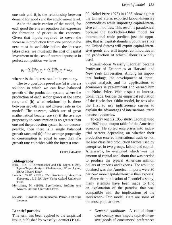
one unit and di is the relationship betweendemand for good i and the employment level.

As in the static version of the model, foreach good there is an equation that expressesthe formation of prices in the economy.Given that inputs required to cover theincrease in production from one period to thenext must be available before the increasetakes place, we must add the cost of capitalinvestment to the cost of current inputs; so inperfect competition we have

pi = ∑j=nj=1aji pj + r∑j=n

j=1bji pj + wli,

where r is the interest rate in the economy.The two questions posed are (a) is there a

solution in which we can have balancedgrowth of the production system, where theproduction of each sector grows at the samerate, and (b) what relationship is therebetween growth rate and interest rate in themodel? The answers, which are of greatmathematical beauty, are (a) if the averagepropensity to consumption is no greater thanone and the production system is non-decom-posable, then there is a single balancedgrowth rate; and (b) if the average propensityto consumption is equal to one, then thegrowth rate coincides with the interest rate.

FRITZ GRAFFE

BibliographyKurz, H.D., E. Dietzenbacher and Ch. Lager, (1998),

Input–Output Analysis, Cheltenham, UK and Lyme,USA: Edward Elgar.

Leontief, W.W. (1951), The Structure of AmericanEconomy, 1919–39, New York: Oxford UniversityPress.

Morishima, M. (1988), Equilibrium, Stability andGrowth, Oxford: Clarendon Press.

See also: Hawkins–Simon theorem, Perron–Frobeniustheorem.

Leontief paradoxThis term has been applied to the empiricalresult, published by Wassily Leontief (1906–

99, Nobel Prize 1973) in 1953, showing thatthe United States exported labour-intensivecommodities while importing capital-inten-sive commodities. This result is paradoxicalbecause the Heckscher–Ohlin model forinternational trade predicts just the oppo-site, that is, capital-abundant countries (likethe United States) will export capital-inten-sive goods and will import commodities inthe production of which labour is widelyused.

Russian-born Wassily Leontief becameProfessor of Economics at Harvard andNew York Universities. Among his impor-tant findings, the development of input–output analysis and its applications toeconomics is pre-eminent and earned himthe Nobel Prize. With respect to interna-tional trade, besides the empirical refutationof the Heckscher–Ohlin model, he was alsothe first to use indifference curves toexplain the advantages of international tradebetween countries.

To carry out his 1953 study, Leontief usedthe 1947 input–output table for the Americaneconomy. He sorted enterprises into indus-trial sectors depending on whether theirproduction entered international trade or not.He also classified production factors used byenterprises in two groups, labour and capital.Afterwards, he evaluated which was theamount of capital and labour that was neededto produce the typical American milliondollars of imports and exports. The result heobtained was that American imports were 30per cent more capital-intensive than exports.

Since the publication of Leontief’s study,many attempts have been made to find an explanation of the paradox that wascompatible with the implications of theHeckscher–Olhin model. Here are some ofthe most popular ones:

• Demand conditions A capital-abun-dant country may import capital-inten-sive goods if consumers’ preferences

Leontief model 153

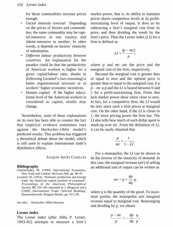
for those commodities increase pricesenough.

• Factor intensity reversal Dependingon the prices of factors and commodi-ties, the same commodity may be capi-tal-intensive in one country andlabour-intensive in another. In otherwords, it depends on factors’ elasticityof substitution.

• Different labour productivity betweencountries An explanation for theparadox could be that the productivityof American workers is higher for agiven capital/labour ratio, thanks to(following Leontief’s own reasoning) abetter organizational structure or toworkers’ higher economic incentives.

• Human capital If the higher educa-tional level of the American workers isconsidered as capital, results maychange.

Nevertheless, none of these explanationson its own has been able to counter the factthat empirical evidence sometimes runsagainst the Heckscher–Ohlin model’spredicted results. This problem has triggereda theoretical debate about the model, whichis still used to explain international trade’sdistributive effects.

JOAQUÍN ARTÉS CASELLES

BibliographyChacholiades, M. (1990), International Economics,

New York and London: McGraw-Hill, pp. 90–97.Leontief, W. (1953), ‘Domestic production and foreign

trade: the American capital position re-examined’,Proceedings of the American PhilosophicalSociety, 97, 331–49; reprinted in J. Bhagwati (ed.)(1969), International Trade: Selected Readings,Harmondsworth: Penguin Books, pp. 93–139.

See also: Heckscher–Ohlin theorem.

Lerner indexThe Lerner index (after Abba P. Lerner,1903–82) attempts to measure a firm’s

market power, that is, its ability to maintainprices above competitive levels at its profit-maximizing level of output. It does so bysubtracting a firm’s marginal cost from itsprice, and then dividing the result by thefirm’s price. Thus the Lerner index (LI) for afirm is defined as

(p – mc)LI = ————,

p

where p and mc are the price and themarginal cost of the firm, respectively.

Because the marginal cost is greater thanor equal to zero and the optimal price isgreater than or equal to the marginal cost, 0 ≤p – mc ≤ p and the LI is bound between 0 and1 for a profit-maximizing firm. Firms thatlack market power show ratios close to zero.In fact, for a competitive firm, the LI wouldbe zero since such a firm prices at marginalcost. On the other hand, if the LI is closer to1, the more pricing power the firm has. TheLI also tells how much of each dollar spent ismark-up over mc. From the definition of LI,it can be easily obtained that

p 1—— = ———.mc 1 – LI

For a monopolist, the LI can be shown tobe the inverse of the elasticity of demand. Inthis case, the marginal revenue (mr) of sellingan additional unit of output can be written as

dpmr = p + —— q,

dq

where q is the quantity of the good. To maxi-mize profits, the monopolist sets marginalrevenue equal to marginal cost. Rearrangingand dividing by p, we obtain

p – mc dp q——— = – —— —,

p dq p

154 Lerner index

where the term on the right-hand side is theinverse of the elasticity of demand (h).Therefore

1LI = —.

h

The less elastic is demand, or the smalleris h, the greater is the difference betweenmarket price and marginal cost of productionin the monopoly outcome, and the mark-upwill increase.

For an industry of more than one but not alarge number of firms, measuring the LI ismore complicated and requires obtainingsome average index. If we assume that thegood in question is homogeneous (so that allfirms sell at exactly the same price), we canmeasure a market-wide LI as

n

p – ∑simcii=1

LI = —————,p

where si is firm i’s market share.From an empirical point of view, there are

practical difficulties in using the Lernerindex as a measure of market power. Themost significant practical obstacle is deter-mining the firm’s marginal cost of produc-tion at any given point in time. A crudeapproximation to the LI which has been usedin the empirical literature is sales minuspayroll and material costs divided by sales,because this magnitude is easy to compute.However, this is not a good approximation inindustries where labour costs are not propor-tional to output because, when output rises,the ratio of labour cost to revenues falls and,ceteris paribus, price–cost margins rise.

JUAN CARLOS BERGANZA

BibliographyLerner, A.P. (1934), ‘The concept of monopoly and the

measurement of monopoly power’, Review ofEconomic Studies, 1 (3), 157–75.

Lindahl–Samuelson public goodsThe Lindahl–Samuelson condition is a theoreti-cal contribution to determine the optimal levelof public goods. This kind of goods presentstwo properties: firstly, non-rivalry in use, thatis, they are not used up when economic agentsconsume or utilize them, and secondly, noexclusion, that is, potential users cannot becostlessly excluded from the consumption ofpublic goods even though they have not paidfor it. Given these characteristics, it can beproved that the competitive equilibrium yieldsan inefficient allocation of this type of goods;that is, a market failure is produced.

The Lindahl–Samuelson contribution hasbecome one of the main blocks of the theoryof public finance, involving issues related towelfare economics, public choice or fiscalfederalism. On the other hand, there aredifferent versions of this rule, depending onwhether distorting taxation is considered,whether a public good provides productiveservices or whether the government pursuesaims different from social welfare.

Assume an economy with two types ofgoods: a private good (X) and a public good(G) that satisfies the properties of no rivalryand no exclusion. Let N be the number ofindividuals who live in that economy. Thepreferences of each individual i are repre-sented by the well-behaved utility functionUi(xi, G), where xi is the individual i’sconsumption of good X. In order to charac-terize the set of Pareto-optimal allocations,we must solve the following problem:

max, U1(x1, G)x1,G

s.t. Ui(xi, G) – u–i ≥ 0, for i = 2, 3, . . ., NF(X, G) = 0.

Assuming that u–i is the minimum utilityconstraint for individual i and F is a strictlyconvex production possibility set, which isnon-decreasing in its arguments, the solutionfor the optimal level of public good G is:

Lindahl–Samuelson public goods 155

N ∂Ui(xi, G)/∂G ∂F/∂G∑—————— = ———.i=1 ∂Ui(xi, G)/∂xi ∂F/∂X

The economic interpretation of thisexpression is straightforward: the efficientquantity of public good G occurs when thesum of the private goods that consumerswould be willing to give up for an additionalunit of the public good just equals the quan-tity of the private good required to producethat additional unit of the public good. Inother words, given the non-rivalry nature ofthe consumption of the public good, the opti-mal level of G must take into account thesum of the marginal rates of substitution ofthe N agents instead of the individualmarginal utility used in the case of theprivate goods. This rule is mainly concernedwith no rivalry of the public goods, while theproperty of no exclusion is not consideredexplicitly. One of the differences betweenSamuelson’s and Lindahl’s approaches is theway they deal with this last characteristic.

The study of the provision of public goodshas been tackled from several theoreticalviewpoints. Although there are authors whohave worked on this topic before, theScandinavian Erik Lindahl was one of thefirst economists to deal with problems of thedecentralized pricing system in order todefine optimally the level of public good tobe provided. Lindahl (1919) suggested atheoretical framework where the preferencesof each agent are revealed through a pseudo-demand curve of a public good. Assumingonly two consumers, the optimal level ofpublic good is determined by the intersectionof the two pseudo-demands; moreover, thissolution shows what price each agent has topay according to the marginal utility hederives from the consumption of the publicgood. The sum of these two prices (the so-called ‘Lindahl prices’) equals the produc-tion cost of the public good.

However, Lindahl’s approach has a crucial

shortcoming: the individuals have no incen-tives to reveal their preferences because theyknow that the price they must pay will dependon the utility they receive. Hence a free-ridersituation appears. Before Lindahl, KnutWicksell proposed that a political processshould be considered in order to know agents’preferences on public goods. Still, there aresubstantial difficulties to designing a well-defined mechanism for voting. Paul A.Samuelson (1954, 1955) was the author whoavoided the free-rider problem and got theoptimal set of solutions for private and publicgoods allocations by means of a benevolentplanner. It is assumed that this omniscientagent knows individual preferences and mayproceed to the efficient solution directly.

Distributional problems about the chargeto finance the public good are solved inSamuelson’s view by applying a socialwelfare function.

DIEGO MARTÍNEZ

BibliographyLindahl, E. (1919), ‘Just taxation – a positive solution’,

reprinted in R.A. Musgrave, and A.T. Peacock (eds)(1958), Classics in the Theory of Public Finance,London: Macmillan.

Samuelson, P.A. (1954), ‘The pure theory of publicexpenditure’, Review of Economics and Statistics,36, 387–9.

Samuelson, P.A. (1955), ‘Diagrammatic exposition of atheory of public expenditure’, Review of Economicsand Statistics, 37, 350–56.

See also: Ledyard–Clark–Groves mechanism.

Ljung–Box statisticsOne aim of time-series modeling, given anobserved series {wt}, is to test the adequacy offit of the model, considering the estimatedresidual series {at}.Usually we assume that thetheoric residuals series {at} is a white noiseand hence that the variables {at} are incorre-lated; the goal of Ljung–Box statistics, intro-duced by these authors in 1978, is to test thisincorrelation starting from the estimators at.

156 Ljung–Box statistics

The model considered by Ljung and Boxis an ARIMA F(B)wt = Q(B)at where F(B) =1 – f1B – . . . – fpBp, Q(B) = 1 – q1B – . . . –qqBq, {at} is a sequence of independent andidentically distributed random variables N(0,s) and {wt} are observable random variables.

If the variables {at} could be observed,we could consider the residual correlationsfrom a sample (a1, . . ., an)

n

∑atat–kt=k+1

rk = ———— (k = 1, . . . m)n

∑at2

t=1

and the statistic

m

Q(r) = n(n + 2)∑(n – k)–1rk2.

k=1

Q(r) is asymptotically distributed as cm2

since the limiting distribution of r = (r1, . . .,rm) is multivariate normal with mean vectorzero,

(n – k)var(rk) = ———

n(n + 2)

and cov(rk, rl) = 0, l ≠ k (Anderson andWalker, 1964).

If the hypotheses of the white noise aretrue, we will expect small rk, and for a signifi-cance level a we will accept the incorrelationhypothesis if Q < cm

2(a).Unfortunately, since the variables {at} are

not observable, we will consider the esti-mated residual series at, obtained from theestimations of the parameters F(B), Q(B),and the residual correlations

n

∑atat–kt=k+1

rk = ———— (k = 1, . . . m),n

∑at2

t=1

introducing finally the Ljung–Box statistic

m

Q(r) = n(n + 2)∑(n – k)–1rk2.

k=1

Ljung and Box proved that, if n is largewith respect to m, E(Q(r)) ≈ m – p – q; thisfact suggested to them that the distribution ofQ(r) might be approximated by the c2

m–p–q.Indeed this approximation and the followingtest which accept the incorrelation hypothe-sis if Q(r) < c2

m–p–q(a), will turn out well inpractice and actually are included in almostevery program about Box–Jenkins method-ology.

PILAR IBARROLA

BibliographyAnderson, T.W. and A.M. Walker (1967), ‘On the

asymptotic distribution of the autocorrelations of asample for a linear stochastic process’, Annals ofMathematical Statistics, 35, 1296–303.

Ljung G.M. and G.E.P. Box (1978), ‘On a measure oflack of fit in time series models’, Biometrika, 65 (2),297–303

Longfield paradox‘The poor are not at all helped as a result ofbeing able to purchase food at half themarket price’ (Johnson, 1999, 676). SamuelMountifort Longfield (1802–84) served as aproperty lawyer and a judge of the Irishcourt. In 1832 he became the first holder ofthe Whatley Chair in Political Economy atTrinity College, Dublin. In his Lectures onPolitical Economy (1834), he deprecated thepractice of trying to help the poor duringtimes of famine by reducing the price ofbasic food, referring to the ancient custom ofcharitable people buying food at the ordinaryprice and reselling it to the poor at a cheaperprice. This action may initially reduce pricesand increase consumption by the poor; butthere will be a feedback effect on marketprice, pushing it up to twice its former level,so the poor pay precisely what they did

Longfield paradox 157

before: ‘Persons of more benevolence thanjudgment purchase quantities of the ordinaryfood of the country, and sell them again tothe poor at half price . . . It induces the farm-ers and dealers to send their stock morespeedily to the market . . . Whenever thismode of charity is adopted, prices will neces-sarily rise’ (Longfield, 1834, pp. 56–7).

LEÓN GÓMEZ RIVAS

BibliographyJohnson, Dennis A. (1999), ‘Paradox lost: Mountifort

Longfield and the poor’, History of PoliticalEconomy, 31 (4), 675–97.

Longfield, Mountifort (1834), Lectures on PoliticalEconomy, Dublin: Richard Milliken and Son.

Lorenz’s curveNamed after Max O. Lorenz (1880–1962),this is a graphical tool that measures thedispersion of a variable, such as income orwealth. This curve is closely related to theGini coefficient. The Lorenz curve is definedas a cumulated proportion of the variable(income or wealth) that corresponds to thecumulated proportion of individuals, increas-ingly ordered by income. Given a sample ofn individuals ordered by income levels, x*

1 ≤x*

2 . . . ≤ x*n, the Lorenz curve is the one that

connects the values (h/n, Lh/Ln), where h = 0,1, 2, . . . n; L0 = 0 and Lh = ∑h

i=1x*i.

Alternatively, adopting a continuous nota-tion, the Lorenz curve can be written as

∫v

0xf(x)dxL(y) = ————,

m

where 0 ≤ y ≤ ∞, and f(y) is the relativedensity function.

The Lorenz curve coincides with thediagonal line (perfect equality line) whenall individuals have the same income level.The Lorenz curve lies below the diagonalline when there exists some incomeinequality. Hence total area between bothcurves would be a potential inequality

measure. In particular, if we multiply thisarea by two, in order to normalize themeasure between zero and one, we obtain theGini coefficient. The Lorenz curve is thebasis for the second-order stochastic orwelfare dominance criterion (Atkinson,1970) and it is commonly used in welfarecomparisons when ranking income distribu-tions.

RAFAEL SALAS

BibliographyAtkinson, A.B. (1970), ‘On the measurement of inequal-

ity’, Journal of Economic Theory, 2, 244–63.Lorenz, M.O. (1905), ‘Methods of measuring concentra-

tion and wealth’, Journal of The AmericanStatistical Association, 9, 209–19.

See also: Atkinson’s index, Gini’s coefficient.

Lucas critiqueIn his seminal work of 1976, Robert E. Lucas(b.1937, Nobel Prize 1995) asserts that macro-econometric models are based on optimalbehaviour or decision rules of economic agentsthat vary systematically with changes in thetime path of government policy variables. Thatis to say, agents’ optimal behaviour dependson their expectations about government deci-sions. Thus traditional economic policy evalu-ation is not possible because the parameters ofmodels are not invariant (that is, the econo-metric models are not structural) and so anychange in policy variables will alter the actualvalue of the estimated parameters. The mainconclusion of Lucas’s work is that policyevaluation in not feasible.

AURORA ALONSO

BibliographyLucas, R.E. Jr. (1976), ‘Econometric policy evaluation:

a critique’, in K. Bruner and A.H. Metzler (eds), ThePhillips Curve and Labor Market, Carnegie-Rochester Conference Series on Public Policy, vol.1, Amsterdam: North-Holland, pp. 19–46.

See also: Muth’s rational expectations.

158 Lorenz’s curve

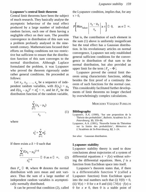
Lyapunov’s central limit theoremCentral limit theorems have been the subjectof much research. They basically analyse theasymptotic behaviour of the total effectproduced by a large number of individualrandom factors, each one of them having anegligible effect on their sum. The possibleconvergence in distribution of this sum was a problem profusely analysed in the nine-teenth century. Mathematicians focused theirefforts on finding conditions not too restric-tive but sufficient to ensure that the distribu-tion function of this sum converges to thenormal distribution. Although Laplaceformulated the problem, it was Lyapunovwho proved the theorem rigorously underrather general conditions. He proceeded asfollows:

Let x1, x2, . . ., xn be a sequence of inde-pendent random variables, with E(xk) = mkand E(xk – mk)

2 = s2k < ∞, and let Fn be the

distribution function of the random variable,

n

∑(xk – mk)k=1————, (1)

sn

where

n

s2n = ∑s2

k.k=1

If there exists a d > 0 such thatn

∑E|xk – mk|2+d

k=1—————— →0 as n →∞, (2)

sn2+d

then Fn → F, where F denotes the normaldistribution with zero mean and unit vari-ance. Thus the sum of a large number ofindependent random variables is asymptoti-cally normally distributed.

It can be proved that condition (2), called

the Lyapunov condition, implies that, for anyt > 0,

xk – mkP[Maxl≤k≤n | ——— | ≥ t] →0, as n →∞.

sn

That is, the contribution of each element inthe sum (1) above is uniformly insignificantbut the total effect has a Gaussian distribu-tion. In his revolutionary articles on normalconvergence, Lyapunov not only establishedgeneral sufficient conditions for the conver-gence in distribution of that sum to thenormal distribution, but also provided anupper limit for the term | Fn – F |.

Lyapunov proved the central limit the-orem using characteristic functions, addingbesides the first proof of a continuity the-orem of such functions for the normal case.This considerably facilitated further develop-ments of limit theorems no longer checkedby overwhelmingly complex calculations.

MERCEDES VÁZQUEZ FURELOS

BibliographyLyapunov, A.A. (1900), ‘Sur une proposition de la

Théorie des probabilités’, Bulletin. Académie Sci. St-Petersbourg, 13, 359–86.

Lyapunov, A.A. (1901), ‘Nouvelle forme du Théorèmesur la limite des probabilités’, Mémoires deL’Académie de St-Petersbourg, 12, 1–24.

See also: Gaussian distribution.

Lyapunov stabilityLyapunov stability theory is used to drawconclusions about trajectories of a system ofdifferential equations x ˘ = f (x) without solv-ing the differential equations. Here, f is afunction from Euclidean space into itself.

Lyapunov’s theorem states that, if there is a differentiable function V (called aLyapunov function) from Euclidean spaceinto the real numbers such that (i) V(0) = 0,(ii) V(x) > 0 for x ≠ 0 and (iii) ∇ V(x) · f (x) ≤0 for x ≠ 0, then 0 is a stable point of

Lyapunov stability 159

the above system of differential equations.Furthermore, if in addition ∇ V(x) · f(x) < 0for x ≠ 0, then 0 is asymptotically stable. Ineither case, the sublevel sets {x: V(x) ≤ a} areinvariant under the flow of f.

The name of Lyapunov is also associatedwith continuum economies, where it guaran-tees the convexity of the aggregate throughthe following result. Let (W, ∑) be a measurespace and let m1, . . ., mn be finite non-atomic

measures on (W, ∑). Then the set{(m1(s), . . .,mn(s)): s ∈ ∑} is compact and convex.

FRANCISCO MARHUENDA

BibliographyM.W. Hirsch and S. Smale (1972), Differential

Equations, Dynamical Systems, and Linear Algebra,Boston, MA: Academic Press.

See also: Negishi’s stability without recontracting.

160 Lyapunov stability

Mann–Wald’s theoremThis theorem extends the conditions underwhich consistency and asymptotic normalityof ordinary least squares (OLS) estimatorsoccur. This result is very useful in econom-ics, where the general regression model iscommonly used. When the regressors arestochastic variables, under the assumptionthat they are independent on the error term,OLS estimators have the same properties asin the case of deterministic regressors: lackof bias, consistency and asymptotic normal-ity. However, a common situation in econo-metric analysis is the case of stochasticregressors which are not independent ofinnovation, for example time series data. Inthese circumstances, OLS estimators losetheir properties in finite samples since theyare biased.

Nevertheless, Henry Berthold Mann(1905–2000) and his master Abraham Wald(1902–50) showed in 1943 that the asymp-totic properties of the OLS estimators holdeven though there is some degree of depen-dence between the regressors and the innova-tion process. A formal state of the theoremcan be found, for example, in Hendry (1995).Mann and Wald’s theorem proves that it ispossible to have consistency and asymptoticnormality for the OLS estimators under thefollowing assumptions: the regressors areweakly stationary, ergodic and contempora-neously uncorrelated with the innovation, andthe innovation is an independently and identi-cally distributed (iid) process with zero meanand finite moments of all orders. In otherwords, the regressors and the error term canbe correlated at some lags and leads, as forexample, with the case where the regressorsare lags of the dependent variable, and stillhave the well known asymptotic properties of

the OLS estimators and therefore the usualinference, OLS standard errors, t statistics, Fstatistics and so on are asymptotically valid.

M. ANGELES CARNERO

BibliographyHendry, D.F. (1995), Dynamic Econometrics, Advanced

Texts in Econometrics, Oxford: Oxford UniversityPress.

Mann, H. and A. Wald (1943), ‘On the statistical treat-ment of linear stochastic difference equations’,Econometrica, 11, 173–220.

Markov chain modelAndrey Andreyevich Markov (1856–1922)introduced his chain model in 1906. Hispaper was related to the ‘weak law of largenumbers’ extension to sums of dependentrandom variables. Markovian dependence isthe key concept. Roughly speaking, itexpresses the view that the current distribu-tion of one random variable, once its entirehistory is known, only depends on the latestavailable information, disregarding the rest.

A chain is defined as any sequence ofdiscrete random variables, and each of itsvalues is a state. The set including all thesestates is called the ‘state space’ (S). If S isfinite, then the chain is said to be a finitechain. Thus a Markov chain will be a chainwith the Markovian dependence as a property.

Formally, let {Xt, t = 0, 1, 2, . . .} be asequence of discrete random variables withvalues in S (state space). It will be a Markovchain when

P(Xt = it/X1 = i1, . . . Xt–1 = it–1) = P(Xt = it/Xt–1= it–1), ∀ t ∈ {1, 2, . . .}, ∀ i1, . . ., it ∈ S.

At each instant t, the chain position isdefined through the state vector

161

M

Vt = (pi(t), i ∈ S), ∀ t ∈ T = {0, 1, 2, . . .],

where pi(t) = P(Xt = i), and the probabilisticdynamic of the model is described by thematrix of transition probabilities:

P(s, t) = (pij(s, t); i, j ∈ S), ∀ s, t ∈ T: s < t, with pij(s, t) = P(Xt = j/Xs = i).

It is easy to prove that the evolution of thestate vector of the Markov chain follows thispattern:

Vt = Vs · P(s, t), ∀ s, t ∈ T: s < t.

One of the most important properties of these transition matrices is theChapman–Kolmogorov equation, commonto all the stochastic processes with theMarkov property. In the above circum-stances,

P(s, t) = P(s, r) · P(r, t), ∀ s, r, t ∈ T: s < r < t.

This fact provides a transition matrixdecomposition into a product of one-steptransition probabilities matrices, by therecursive use of the Chapman–Kolmogorovequation,

P(s, t) = P(s, s + 1) · P(s + 1, s + 2) · . . . ·P(t – 1, t) ∀ s, t ∈ T: s < t.

It is very useful to assume that one-step tran-sition probabilities are invariant across time.In such a case, the Markov chain will becalled homogeneous;

P(t, t + 1) = P, ∀ t ∈ T, and soVt = V0 · Pt, ∀ t ∈ T,

and the whole dynamic of the model can bedescribed using only V0 and P.

Nevertheless, the easiest case is deter-mined when the one-step transition matrix is

a regular one (each state is accessible fromthe others in a given number of steps). Asimple sufficient condition is that all theelements of the one-step transition matrix arestrictly positive. In such a case, the Markovchain model is called ergodic; that is, itreaches a stationary limit distribution.Formally,

p · P = p; ∑pi = 1 satisfies:i∈ S

lim Vt = lim V0 · Pt = p,t→∞ t→∞

whatever the initial state vector (V0) is, andthe convergence rate is geometric.

There are more complex models ofMarkov chains, according to the accessibilitycharacteristics of the states, such as the per-iodic and reducible cases. On the other hand,the extension to time-continuous Markovchains is not difficult. Furthermore, themodel displayed here is the first-order one,whereas the high-order extension is alsopossible.

Markov chain models may be consideredas a very versatile tool and they have beenemployed in many fields, including success-ful applications in economics and sociology,among others.

JOSÉ J. NÚÑEZ

BibliographyMarkov, A.A. (1906), ‘Rasprostraneniye zakona

bol’shikh chisel na velichiny, zavisyashchiye drug otdruga’ (Extension of the law of large numbers toquantities dependent on each other), Izvestiya Fiz.-Matem. o-va pro Kazanskom un-te (2), 15, 135–56.

Parzen, E. (1962), Stochastic Processes, San Francisco:Holden-Day.

Markov switching autoregressive modelMany macroeconomic or financial time seriesare characterized by sizeable changes in theirbehaviour when observed for a long period.For example, if the series is characterized byan AR (1) process whose unconditional mean

162 Markov switching autoregressive model

changes after period T*, then prior to T* wemight use the model

yt – m1 = r(yt–1 – m1) + et,

whereas after T* the corresponding model is

yt – m2 = r(yt–1 – m2) + et,

where I r I < 1 and m1 ≠ m2 and et, is an iiderror term.

Since the process has changed in the past,the prospect that it may change in the futureshould be taken into account when construct-ing forecasts of yt. The change in regimeshould not be regarded as the outcome of a foreseeable determinist event. Thus acomplete time series model would include adescription of the probability law governingthe regime change from m1 to m2. This obser-vation suggests considering an unobservedrandom state variable, st

*, which takes twovalues (say, 0 and 1), determining underwhich regime is the time series (say, state 1with m = m1 or state 2 with m = m2), so that themodel becomes

yt – m (st*)= r[yt–1 – m(st

*)] + et.

Hamilton (1989) has proposed modelling(st

*) as a two-state Markov chain with prob-abilities pij of moving from state i to state j (i,j = 1, 2). Thus p12 = 1 – p11 and p21 = 1 – p22.Interpreting this model as a mixture of twodistributions, namely N(m1, s2) and N(m2, s2)under regimes 1 and 2, respectively, the EMoptimization algorithm can be used to maxi-mize the likelihood of the joint density of ytand st

* given by f (yt, st* = k, q) with k = i, j and

q = {m1, m2, r, s2}.This modelling strategy, known as the

Markov switching (MS) autoregressivemodel, allows us to estimate q and the transi-tion probabilities so that one can computeforecasts conditions in any given state. Thebasics of the procedure can also be extended

to cases where r1 ≠ r2 and s21 ≠ s2

2, and tomultivariate set-ups. A useful application ofthis procedure is to estimate the effect of onevariable on another depending on the busi-ness cycle phase of the economy.

JUAN J. DOLADO

BibliographyHamilton, J.D. (1989), ‘A new approach to the study of

nonstationary time series and the business cycle’,Econometrica, 57, 357–84.

Markowitz portfolio selection modelHarry Markowitz (b.1927, Nobel Prize 1990)presented in his 1952 paper the portfolioselection model, which marks the beginningof finance and investment theory as we knowit today. The model focuses on rational deci-sion making on a whole portfolio of assets,instead of on individual assets, thus concern-ing itself with total investor’s wealth.

The mathematical formulation is asfollows. Consider a collection of individualassets (securities) and their returns at theend of a given time horizon, modelled asrandom variables characterized by theirrespective means and their covariancematrix. Markowitz hypothesized a mean-variance decision framework: investorsfavour as much expected return as possible,while considering variance of returns asnegative. Risk (what investors dislike inreturns) is identified with variance. Theproblem is to determine what are rationalportfolio choices, where a portfolio isdefined by a set of weights on individualassets. In this decision, rational investorswould only be concerned with their final(end of horizon) wealth. The desired portfo-lios should provide the highest possibleexpected return given a maximum level ofadmissible portfolio variance, and (dually)the minimum possible variance given arequired level of expected return.

Markowitz saw that the solution was not a

Markowitz portfolio selection model 163

single portfolio, but that there would be a setof efficient portfolios (the ‘efficient frontier’)fulfilling these conditions. In order tocompute the solution, it is necessary to solvea set of quadratic programming problemssubject to linear constraints, a demandingtask at the time but amenable today to veryefficient implementation.

Markowitz himself extended the originalmodel in his 1959 book, addressing thechoice by an individual investor of onespecific optimal portfolio along the efficientfrontier, and had the insight on which Sharpewould later build in developing a simplified(single-index) version of the model. Muchacademic work in finance followed, byTobin among many others.

The economic significance of Markowitz’scontribution is paramount. His is both arigorous and an operational model that quan-tifies risk and introduces it on an equal foot-ing with expected return, hence recognizingthe essential trade-off involved betweenthem. Also, as a result of the model, the vari-ability of returns from an individual asset isdistinguished from its contribution to portfo-lio risk, and full meaning is given to theconcept of diversification: it is important notonly to hold many securities, but also toavoid selecting securities with high covari-ances among themselves.

It has been argued that the practicalimpact of the Markowitz model on actualportfolio construction does not rank as highas its theoretical significance. The model’smain practical shortcomings lie in the diffi-culty of forecasting return distributions, andin that, often, the model yields unintuitivesolutions, which happen to be very sensitiveto variations in the inputs. Also both theidentification of risk with variance and thehypothesis of investor rationality have beenquestioned. Nevertheless, the conceptualwork initiated by Markowitz is either a foun-dation or a reference for departure on whichto base any practical methods, thus securing

its place as a classic in both theory and prac-tice. In 1990, Markowitz was awarded, thefirst Nobel Prize in the field of financialeconomics, fittingly shared with Sharpe (andMiller).

GABRIEL F. BOBADILLA

BibliographyMarkowitz, H.M. (1952), ‘Portfolio selection’, Journal

of Finance, 7, 77–91.Markowitz, H.M. (1959), Portfolio Selection: Efficient

Diversification of Investments, New York: Wiley.

Marshall’s external economiesAlfred Marshall (1842–1924), Professor ofPolitical Economy at the University ofCambridge, was the great link between clas-sical and neoclassical economics. He was thefounder of the Cambridge School ofEconomics and Pigou and Keynes wereamong his pupils. Marshall’s Principles ofEconomics (1890) was for many years theBible of British economists, introducingmany familiar concepts to generations ofeconomists.

His industrial district theory relies on theconcept of external economies: when firmsin the same industry concentrate in a singlelocality, they are more likely to lower cost ofproduction. External economies encouragethe specialized agglomeration of firms byincreasing the supply of inputs. The largerthe supply, the lower the costs of productionto all the firms in the locality. So each firm inthe area becomes more competitive than if itoperated on its own. This concentration ofmany small businesses with similar charac-teristics can be an alternative to a larger sizefor the individual firm (internal economies).

But Marshall went one step further. Hestated that these industrial gatherings createsomething ‘in the air’ (Marshall’s words)that promotes innovation. This environmentof geographic proximity and economicdecentralization provides an ‘industrialatmosphere’ to exchange ideas and develop

164 Marshall’s external economies

skills within the district. The interaction ofbuyers, sellers and producers gives rise to‘constructive cooperation’. Constructivecooperation allows even small businesses tocompete with much larger ones.

Marshall’s industrial theory has been rein-terpreted many times as an explanation ofnew behaviours after the mass productionstage. Rival firms manage to cooperatearound activities of mutual benefit such asmarket research and development, recruit-ment and training processes or commonmarketing campaigns.

MANUEL NAVEIRA

BibliographyMarshall, A. (1890), Principles of Economics: an

Introductory Text, London; Macmillan and Co.,Book IV, chs. X and XI.

Marshall’s stabilityAlfred Marshall (1842–1924) developed hisanalysis of market stability in two essayswritten in 1879, one on the theory of foreigntrade and the other on the theory of domesticvalues. Both were printed for private circula-tion and partially included later in hisPrinciples (Marshall, 1890, bk 5, chs. 11, 12and app. H).

Marshall’s interest in market stability aroseas a consequence of his awareness of the diffi-culties posed by the existence of increasingreturns for the existence of a long-run competi-tive equilibrium solution. He believed that anegatively sloped supply curve was notunusual in many industries. Significantly, hediscussed stability in an appendix entitled‘Limitations of the use of statical assumptionsin regard to increasing returns.’

The Marshallian stability analysis hasthree main characteristics. The first is that itis formulated in terms of the equilibrium of asingle market, without taking into accountthe reaction of markets other than the oneunder consideration. The second is that theexcess demand price, defined as the differ-

ence between demand and supply prices,governs the response of output and not theother way round. Modern stability analysisfollows Hicks (1939) in adopting the viewthat the price response is governed by excessdemand. Finally, the market-clearing processdoes not take place in the short run. ForMarshall it takes place in the long runbecause of the changes required in the firms’scale of production.

Consider an initial equilibrium positionand let output fall. If the new demand price ishigher than the supply price, firms selling atthe former would earn above-normal profits.In that case incumbent firms would raisetheir production levels and new capitalwould accrue to the productive sector.Consequently, total output would rise and themarket would go back to the initial (stable)equilibrium.

The stability condition is stated byMarshall as follows: ‘The equilibrium ofdemand and supply [. . .] is stable or unstableaccording as the demand curve lies above orbelow the supply curve just to the left of thatpoint or, which is the same thing, accordingas it lies below or above the supply curve justto the right of that point’ (Marshall, 1890,app. H, p. 807, n). If the demand curve isalways negatively sloped, this implies thatthe market equilibrium is stable when thesupply curve has a positive slope. However,when the supply curve has a negative slope,the Marshallian stability condition is theopposite of the standard one stated in termsof the slope of the excess demand function.That was the reason why Hicks (1939, p. 62)considered that Marshallian analysis is notconsistent with perfect competition. How-ever, it would be quite appropriate undermonopoly, since in that case an equilibriumposition is stable when a small reduction inoutput makes marginal revenue greater thanmarginal cost.

JULIO SEGURA

Marshall’s stability 165

BibliographyHicks, J.R. (1939), Value and Capital, Oxford: Oxford

University Press (2nd edn 1946).Marshall, A. (1879), ‘The Pure Theory of Foreign

Trade’ and ‘The Pure Theory of Domestic Values’,reprinted together in 1930 as no. 1 in Series ofReprints of Scarce Tracts in Economic and PoliticalScience, London School of Economics and PoliticalScience.

Marshall, A. (1890), Principles of Economics: AnIntroductory Text, London: Macmillan.

See also: Hicksian perfect stability.

Marshall’s symmetallismThis is a bimetallic currency scheme,‘genuine and stable’ as it was assessed byAlfred Marshall ([1887] 1925, p. 204), basedon the gold standard system proposed byDavid Ricardo in his Proposals for anEconomical and Secure Currency (1816) butdiffering from his ‘by being bimetallicinstead of monometallic’ (Marshall [1887]1925, pp. 204–6; 1923, pp. 65–7; 1926, pp.28–30).

Marshall’s symmetallism is a system ofpaper currency, exchangeable on demand atthe Mint or the Issue Department of the Bankof England for gold and silver, at the sametime, at the rate of one pound for 56½ grainsof gold together with 20 times as manygrains of silver. This proportion betweengold and silver established by Marshall wasstable but not precise. In fact, in a manuscriptnote written in the margin of a page of hiscopy of Gibbs’s The Double Standard(1881), Marshall proposed a rate of n of goldand 18n of silver (Marshall [1887] 1925, p.204; Eshag 1963, p. 115n). The proportionwould be fixed higher or lower depending onwhether one wished to regulate the value ofcurrency chiefly by one or other metal. ‘Butif we wished the two metals to have aboutequal influence,’ we should take account ofthe existing stocks of the two metals(Marshall [1887] 1925, p. 204n; 1926, p. 29)and the changes in their productions.Anyway, the rate would be fixed once andfor all. Marshall, finally, proposed that a bar

of 100 grammes of gold and a silver bar 20times as heavy would be exchangeable forabout £28 or £30 (Marshall [1887] 1925, pp.204–5). He proposed to make up the goldand silver bars in gramme weights ‘so as tobe useful for international trade’ (ibid., p.204; 1923, pp. 64, 66; 1926, p. 14).

The proposal differs from other bimetallicsystems that exchange paper currency forgold or silver at a fixed ratio of mintage (orcoinage) closely connected to the relativevalues of the metals in the market; these arenot really bimetallic because, when the valueof one metal, usually gold, increases to ahigh level in relation to the other, because thecost of mining and producing gold is goingup relatively to that of silver, assuming thatthe demand of both metals is the same duringthe process, then bimetallism works asmonometallism, usually of silver. In fact,Marshall did not defend bimetallic plans,including the best (his symmetallism),because he believed that in practice they donot contribute to stabilizing prices muchmore than monometallism (Marshall [1887]1925, pp. 188, 196; 1926, pp. 15, 27–8,30–31).

FERNANDO MÉNDEZ-IBISATE

BibliographyEshag, Eprime (1963), From Marshall to Keynes. An

Essay on the Monetary Theory of the CambridgeSchool, Oxford: Basil Blackwell.

Marshall, Alfred (1887), ‘Remedies for fluctuations ofgeneral prices’, reprinted in A.C. Pigou (ed.) (1925),Memorials of Alfred Marshall, London: Macmillan,and (1966) New York: Augustus M. Kelley.

Marshall, Alfred (1923), Money Credit and Commerce,reprinted (1965) New York: Augustus M. Kelley.

Marshall, Alfred (1926), Official Papers by AlfredMarshall, London: Macmillan.

Marshallian demandAlfred Marshall (1842–1924) was an out-standing figure in the development ofcontemporary economics. He introducedseveral concepts that became widely used in

166 Marshall’s symmetallism

later analysis. His most famous work,Principles of Economics, first published in1890, went through eight editions in his life-time. Although incomplete, his treatment ofdemand had a great influence on later devel-opments of consumer theory. He introducedconcepts such as the consumer surplus anddemand elasticity, and set the framework forthe analysis of consumer behaviour. As atribute to his pioneering contribution, theordinary demand functions derived fromconsumers’ preferences taking prices andwealth as given are known as Marshalliandemand functions.

In the standard demand theory, it isassumed that consumers have rational,convex, monotone and continuous prefer-ences defined over the set of commoditybundles x∈ Rn

+. Under these assumptions,there exists a continuous, monotone andstrictly quasi-concave utility function u(x)that represents these preferences. Theconsumer maximizes her utility taking theprice vector p ∈ Rn

++ and wealth level w > 0as given. Hence the utility maximizationproblem can be specified as follows:

Max u(x)x≥0

s.t. px ≤ w.

If u(x) is continuously differentiable, thefirst-order conditions for an interior solutionare

Ui(x) Uj(x)m = ——— = ——— (i, j = 1, . . ., n),

pi pj

where m is the Lagrange multiplier of theoptimization problem. Under the aboveassumptions, the solution to this problemexists. The optimal consumption vector isdenoted by x(p, w) ∈ Rn

+ and is known as theMarshallian (or ordinary) demand function.In equilibrium, the price-adjusted marginalutility of the last unit of wealth spent in each

commodity must equal the Lagrange multi-plier m, which is the constant marginal utilityof wealth. Hence the equilibrium conditionimplies that the marginal rate of substitutionof two arbitrary goods i and j must equal therelative price of both goods.

The Marshallian demand function is homo-geneous of degree zero in (p, w), since thebudget set does not change when prices andwealth are multiplied by a positive constant.Moreover, in equilibrium it must hold that px= w, because of the assumption of monotonepreferences (Walras’s law holds). Finally, as itis assumed that p >> 0 and w > 0 (hence, thebudget set is compact) it is possible to showthat x(p, w) is a continuous function.

XAVIER TORRES

BibliographyMarshall, A. (1920), Principles of Economics, London:

Macmillan.Mas-Colell, A., M.D. Whinston and J.R. Green (1995),

Microeconomic Theory, Oxford: Oxford UniversityPress.

See also: Hicksian demand, Slutsky equation.

Marshall–Lerner conditionThe condition is so called in honour ofAlfred Marshall (1842–1924) and Abba P.Lerner (1903–1982), the condition estab-lishes that, starting from an equilibrium inthe current account of the balance ofpayments, a real exchange rate depreciationproduces a current account surplus only if thesum of the price elasticities of the export andimport demands of a country, measured inabsolute values, is greater than one. If thestarting point is a disequilibrium, measuredin national currency units, it is required thatthe ratio of exports to imports multiplied bythe price elasticity of the exports demandplus the price elasticity of the importsdemand be greater than one.

Usually, a country (A) devalues becauseits balance of trade shows a deficit. A rise in

Marshall–Lerner condition 167

the real exchange rate, or a devaluation,generally makes foreign products moreexpensive in relation to home products, andso imports expressed in foreign currencytend to decrease. But a devaluation influ-ences A’s export earnings too. For the rest ofthe world, the decrease in A’s export pricesincreases their purchases, and A’s exports.These changes seem to assure an improve-ment in the current account and stability inthe exchange market, but this reasoning hasassumed that both A’s import and exportdemands are elastic, so the reactions of totalexpenditure on exports and imports are morethan proportional to the changes of theirrespective relative prices or of the realexchange rate. If foreign demand is inelastic,the export earnings of A will not increase andthey could even diminish in a greater propor-tion than the fall in A’s import expenses. Theresult will be a larger trade deficit and moreinstability in the exchange rate market. On the other hand, although the volumeimported by A falls in terms of units offoreign products, it could happen that, afterthe devaluation, imports measured in units ofnational product increase because the deval-uation tends to increase the value of everyunit of product imported by A in terms ofunits of A’s national product. In this way itseffect on the trade balance will remain uncer-tain.

FERNANDO MÉNDEZ-IBISATE

BibliographyChacholiades, Miltiades (1990), International

Economics, 2nd edn, New York: McGraw-Hill.Lerner, Abba P. (1944), The Economics of Control.

Principles of Welfare Economics, New York:Macmillan, pp. 356–62, 377–80, 382–7.

Marshall, Alfred (1879), ‘The pure theory of foreigntrade’, printed privately; reprinted (1974) with ‘Thepure theory of domestic values’, Clifton, NJ:Augustus M. Kelley, pp. 9 (particularly footnote) –14, 18–28.

Marshall, Alfred (1923), Money Credit and Commerce;reprinted (1965) New York: Augustus M. Kelley.

Maskin mechanismA social choice rule (SCR) maps preferencesinto optimal allocations. A SCR is monot-onic if whenever chooses allocation A itkeeps the same choice when A is equally ormore preferred in the ranking of all agents.An SCR satisfies no veto power if it choosesA when A is top ranking for, at least, allagents minus one.

A mechanism is a message space and afunction mapping messages into allocations.A mechanism implements an SCR in NashEquilibrium (NE) if for any preferenceprofile optimal allocations coincide withthose yielded by NE.

Maskin conjectured that, with more thantwo agents, any SCR satisfying monotonicityand no veto power was implementable inNE. He constructed a ‘universal mechanism’to do the job. This is the Maskin mechanism.Even though the spirit was correct, the origi-nal proof was not. Repullo, Saijo, Williamsand McKelvey offered correct proofs.

In the Maskin mechanism each agentannounces the preferences of all agents, anallocation and an integer. There are threepossibilities. The first is complete agreement:all agents announce the same preferences andallocation and this allocation is optimal forthe announced preferences. The allocation isthe one announced by everybody.

The second possibility is a single dissi-dent: a single agent whose announcementdiffers from the others. The allocation cannotimprove the dissident’s payoff if her prefer-ences were announced by others. The thirdpossibility is several dissidents: severalagents whose messages differ. The allocationis announced by the agent whose message isthe highest integer.

The interpretation of the mechanism isthat the dissident must prove that she is notmanipulating the mechanism in her favour,but pointing out a plot of the other agents tofool the mechanism. With several dissidents,the ‘law of the jungle’ holds.

168 Maskin mechanism

This mechanism has been critized becausethe strategy space is not bounded (if bounded,there might be NE yielding suboptimal allo-cations) and because, with several dissidents,allocations are dictatorial (if agents renegoti-ated these allocations, there might be NEyielding suboptimal allocations).

Experiments run with this mechanismsuggest that both criticisms are far from themark. The true problem is that to become asingle dissident might be profitable andnever hurts. If this deviation is penalized, thefrequency of suboptimal NE is about 18 percent.

LUÍS CORCHÓN

BibliographyMaskin, E. (1999), ‘Nash equilibrium and welfare opti-

mality’, Review of Economic Studies, 66, 23–38;originally published with the same title as an MITmimeo, in 1977.

Minkowski’s theoremHermann Minkowski (1864–1909) was bornin Russia, but lived and worked mostly inGermany and Switzerland. He received hisdoctorate in 1884 from Königsberg andtaught at universities in Bonn, Königsberg,Zurich and Göttingen. In Zurich, Einsteinwas a student in several of the courses hegave. Minkowski developed the geometricaltheory of numbers and made numerouscontributions to number theory, mathemat-ical physics and the theory of relativity. Atthe young age of 44, he died suddenly from aruptured appendix. Students of analysisremember Minkowski for the inequality thatbears his name, relating the norm of a sum tothe sum of the norms.

The standard form of Minkowski’s in-equality establishes that the Lp spaces arenormed vector spaces. Let S be a measurespace, let 1 ≤ p ≤ ∞ and let f and g beelements of Lp(S). Then f + g ∈ Lp(S) and

|| f + g ||p ≤ || f ||p + || g ||p

with equality if and only if f and g arelinearly dependent.

The Minkowski inequality is the triangleinequality in Lp(S). In the proof, it is suffi-cient to prove the inequality for simple func-tions and the general result that follows bytaking limits.

The theorem known as Minkowski’sseparation theorem asserts the existence of ahyperplane that separates two disjointconvex sets. This separation theorem is probably the most fundamental result inmathematical theory of optimization whichunderlies many branches of economictheory. For instance, the modern approachfor the proof of the so-called ‘second theorem of welfare economics’ invokesMinkowski’s separation theorem for convexsets. The theorem is as follows.

Let A and B be non-empty convex subsetsof Rn such that A ∩ B = ∅ . Then there existsa hyperplane separating A and B; that is,there exists a point p∈ Rn such that

sup p · x ≤ inf p · xx∈ A x∈ B

If, in addition, A is closed and B is compact,we can strengthen the conclusion of the the-orem with strict inequality.

One of the important applications of sep-aration theorems is the Minkowski–Farkaslemma, as follows. Let a1, a2, . . ., am and b ≠0 be points in Rn. Suppose that b · x ≥ 0 forall x such that ai · x ≥ 0, i = 1, 2, . . ., m. Thenthere exist non-negative coefficients l1, l2, . . ., lm, not vanishing simultaneously, suchthat

b = ∑mi=1liai.

The Minkowski–Farkas lemma plays animportant role in the theory of linearprogramming (for example, the duality the-orem), game theory (for example, the zero-sum two-person game), and the theory of

Minkowski’s theorem 169

nonlinear programming (for example, theKuhn–Tucker theorem).

EMMA MORENO GARCÍA

BibliographyHildenbrand, W. (1974), Core and Equilibria of a Large

Economy, Princeton, NJ: Princeton University Press.Minkowski, H. (1896), Geometrie der Zahlen, vol. 1,

Leipzig: Teubner, pp. 115–17.Takayama, A. (1985), Mathematical Economics, 2nd

edn, Cambridge: Cambridge University Press.

See also: Kuhn–Tucker theorem.

Modigliani–Miller theoremThis famous theorem is formulated in twointerrelated propositions. Proposition I estab-lishes that the total economic value of a firmis independent of the structure of ownershipclaims, for example between debt and equity.The proposition holds under reasonablygeneral conditions and it had a big impact inthe economics and finance literature becauseit implies that corporate finance, at least as itrelates to the structure of corporate liabilities,is irrelevant to determining the economicvalue of the assets of the firm. One importantcorollary of the proposition is that firms canmake the investment decisions indepen-dently of the way such investment will befinanced.

A few years after the first paper waspublished, Franco Modigliani (1918–2003,Nobel Prize 1985) and Merton H. Miller(1923–2000, Nobel Prize 1990) extendedproposition I to the claim that the dividendpolicy of firms is irrelevant in determiningtheir economic value, under the same condi-tions that make irrelevant the financial struc-ture.

One way to present the argument is tosuppose that the firm divides its cash flowsarbitrarily into two streams and issues titles toeach stream. The market value of each titlewill be the present discounted value of thecorresponding cash flows. Adding the values

of the two assets gives the discounted valueof the original undivided stream: the totalvalue of the firm is invariant to the way prof-its are distributed between different claims.The conclusion applies to the divisionbetween debt and equity claims, but also tothe division between different types of equity(ordinary or preferred) and between differenttypes of debt (short-term or long-term). Butin their original paper the authors proved theproposition in a more straightforward way: inperfect capital markets where individualinvestors can borrow and lend at the samemarket rates as business firms, no investorwill pay a premium for a firm whose financialstructure can be replicated by borrowing orlending at the personal level. This basic resulthas been useful for identifying other decis-ions of firms that do not create economicvalue: for example, if firms divest their assetsin a pure financial way so that personalinvestors can replicate the same diversifica-tion in their portfolio of investments.

In a perfect capital market the financingdecisions do not affect either the profits ofthe firm or the total market value of theassets. Therefore the expected return onthese assets, equal to the profits divided bythe market value, will not be affected either.At the same time, the expected return on aportfolio is equal to the weighted average ofthe expected returns of the individual hold-ings, where the weights are expressed inmarket values.

When the portfolio consists of the firm’ssecurities, debt and equity, from the equationdefined above one can solve for the expectedreturn on the equity, rE, of a levered firm asa function of the expected return on the totalassets, rA, the expected return on debt, rD,and the debt/equity ratio, D/E, both at marketvalues,

DrE = rA + (rA – rD) —.E

170 Modigliani–Miller theorem

This is Modigliani and Miller propositionII: the expected rate of return on the stock ofa leveraged firm increases in proportion tothe debt/equity ratio expressed in marketvalues; the increase is proportional to thespread between rA, the expected return of theproductive assets, and rD, the expected returnon debt.

The expected rate of return on equity, rE,is the cost of capital for this form of financ-ing, that is, the minimum expected rate ofreturn demanded by investors to buy theasset. With no debt, D = 0, this expectedreturn is just the expected return demandedto the productive assets, as a function of theirstochastic characteristics (economic risk)and of the risk-free interest rate. Leverageincreases the risk of the shares of the firmbecause the interest payment to debt is fixed and independent of the return on the assets. The debt/equity decision amplifies thespread of percentage returns for the shares ofthe firm, and therefore the variability of suchreturns, compared with the variability withno debt in the financial structure. The cost ofequity capital for the levered firm increasesto compensate shareholders for the increasein the risk of their returns due to the issue ofcorporate debt.

Modigliani and Miller propositions holdwhen the division of the cash flows gener-ated by the productive assets of the firm doesnot affect the size of total cash flows. Thereare at least two reasons why this may not bethe case. The first is the fact that interestpayments to debt holders are not taxed at thecorporate level. A shift from equity to debtfinance therefore reduces the tax burden andincreases the cash flow. The second is thatthere may be bankruptcy costs. Bankruptcyis a legal mechanism allowing creditors totake over when a firm defaults. Bankruptcycosts are the costs of using this mechanism.These costs are paid by the stockholders andthey will demand compensation in advancein the form of higher pay-offs when the firm

does not default. This reduces the possiblepay-off to stockholders and in turn reducesthe present market value of their shares.

As leverage increases, the market value ofthe firm increases with the present value oftax savings and decreases with the increasingexpected bankruptcy costs. At some point themarket value will reach a maximum whichwill correspond to the optimal leverage ratio.This is the first extension of the Modiglianiand Miller world to the case where institu-tional and regulatory interventions in themarket create imperfections that determinethe relevance of the financial decisions.Other extensions have to do with the pres-ence of information asymmetries betweenshareholders, managers and creditors whichcreate incentive problems and new opportu-nities to link wealth creation with financialdecisions.

VICENTE SALAS

BibliographyMiller, M.H. and F. Modigliani (1961), ‘Dividend

policy, growth and the valuation of shares’, Journalof Business, 34 (4), 411–41.

Modigliani, F. and M.H. Miller (1958), ‘The cost ofcapital, corporation finance and the theory of invest-ment’, American Economic Review, 48 (3), 261–97.

Montaigne dogmaThe gain of one man is the damage ofanother. Ludwig von Mises coined theeponym in Human Action, referring to theFrench writer Michel E. de Montaigne(1533–92), who wrote: ‘let every man soundhis owne conscience, hee shall finde that ourinward desires are for the most part nour-ished and bred in us by the losse and hurt ofothers; which when I considered, I began to thinke how Nature doth not gainesayherselfe in this, concerning her generall policie: for Physitians hold that the birth,increase, and augmentation of everything, isthe alteration and corruption of another’.Mises restated the classical anti-mercantilist

Montaigne dogma 171

doctrine according to which voluntary marketexchanges are not exploitation or zero-sumgames, and said: ‘When the baker providesthe dentist with bread and the dentist relievesthe baker’s toothache, neither the baker northe dentist is harmed. It is wrong to considersuch an exchange of services and the pillageof the baker’s shop by armed gangsters as twomanifestations of the same thing.’

GORKA ETXEBARRIA ZUBELDIA

BibliographyMises, Ludwig von (1996), Human Action, 4th rev. edn,

San Francisco: Fox & Wilkes, pp. 664–6.Montaigne (1580), Essais, reprinted F. Strowski (ed.)

(1906), Bordeaux, bk I, ch. 22, pp. 135–6. Englishtranslation by John Florio (1603), London: Val.Sims for Edward Blount.

Moore’s lawThe electronic engineer Gordon E. Moore, co-founder of Intel, observed in 1965 that, in inte-grated circuits, the transistor density or ‘thecomplexity for minimum component costs hasincreased at a rate of roughly a factor of twoper year; certainly over the short term this ratecan be expected to continue, if not toincrease’. The press called this ‘Moore’s law’,and in fact the doubling every eighteenmonths was the pace afterwards. Economistsstudying the Internet, such as MacKie-Masonand Varian, have observed that ‘the traffic onthe network is currently increasing at a rate of6 per cent a month, or doubling once a year’,and that ‘the decline in both communicationslink and switching costs has been exponentialat about 30 per cent per year’.

CARLOS RODRÍGUEZ BRAUN

BibliographyMacKie-Mason, Jeffrey and Hal R. Varian, (1995),

‘Some economics of the Internet’, in Werner Sicheland Donald L. Alexander, (eds), Networks,Infrastructure and the New Task for Regulation,Ann Arbor: University of Michigan Press.

Moore, Gordon E. (1965), ‘Cramming more compo-nents onto integrated circuits’, Electronics, 38 (8),April.

Mundell–Fleming modelThis is an extension of the closed economyIS–LM model to deal with open economymacroeconomic policy issues. There are twoways in which the IS–LM model isexpanded. First, it includes the term ‘netexports’ (NX) in the IS curve. Second, it addsa balance of payments equilibrium conditionin which net exports equal net foreign invest-ment (NFI). The latter is a function of thedomestic interest rate (r), the foreign interestrate (r*) and the exchange rate (e), followingthe interest rate parity condition. Prices areassumed to be fixed, both domestically andinternationally.

The balance of payments equilibriumcondition states that any current accountunbalance must be matched with a capitalaccount surplus and vice versa. From thisequilibrium condition there can be derived aBP curve in the (r, Y) space in which theIS–LM model is represented.

Formally, making exports depend onforeign output, imports depend on domesticoutput and both on the exchange rate, theequilibrium balance of payment conditioncan be written as

NX (e, Y, Y*) = NFI (r, r*)

which can be rewritten as r = BP(Y).The BP curve in the figure is an increas-

ing function, with a smaller slope than theLM’s (important for stability). The exchangerate is given along the BP curve. Any pointabove the BP curve means that the economyis in a balance of payments surplus, thecontrary applying below it. When the IS andthe LM curves, representing the domesticequilibrium, intersect above the BP curve,the adjustment will come via an appreciationof the exchange rate under a floatingexchange rate regime, or via an inflow ofcapital and foreign reserves and the corre-sponding monetary expansion, shifting theLM to the right, if the economy has a fixed

172 Moore’s law

exchange rate regime. A small economyversion of this model may be written with r =r* and the BP curve being flat.

The main conclusions of the Mundell–Fleming model are the following. An expan-sionary fiscal policy will raise interest ratesand output under a fixed exchange rateregime and, besides these, will appreciate thecurrency in a floating exchange rate regime.An expansionary monetary policy has nopermanent effects under a fixed exchangerate regime (reserves are limited) and willlower interest rates, increase income anddepreciate the currency under a floatingregime. Further expansions of the Mundell–Fleming model included price variability.

The Mundell–Fleming model was devel-oped in the early 1960s. Interestingly, therewas no joint work of the two authors. Boththe Robert A. Mundell (b.1932, NobelPrize 1999) and the J. Marcus Fleming(1911–76) original papers were publishedin 1962, although Mundell’s contributionsto the model are collected in four chaptersof Mundell (1968), following his ‘rule’(‘one idea, one paper’). The reason why it

is called ‘Mundell–Fleming’ instead of‘Fleming–Mundell’ is that Mundell’s workwas pioneering and independent of Fleming’s,the converse not being true, although bothof them worked for the IMF at that time.

MIGUEL SEBASTIÁN

BibliographyFleming, J.M. (1962), ‘Domestic financial policies

under floating exchange rates’, IMF Staff Papers, 9,369–72.

Mundell, R.A. (1968), ‘The appropriate use of fiscal andmonetary policy under fixed exchange rates’, IMFStaff Papers, 9, 70–77.

Mundell, R.A. (1968), International Economics, NewYork: Macmillan.

See also: Hicks–Hansen model.

Musgrave’s three branches of the budgetThis originated in a methodological artificeof great pedagogical utility, still viable today,devised in 1957 by Richard Musgrave(b.1910). In that contribution a pattern wasconfigured, based on which the process ofrevenue and public expenditure could beanalyzed in mixed market economies. This

Musgrave’s three branches of the budget 173

LM

BP

IS

Y

r

Mundell-Fleming model

position attempts to respond to a simple butradical question: why in these economies didan important part of the economic activityhave its origin in the public sector’s budget?

Musgrave outlines a theory of the optimalbudget where, in answer to this query, heaffirms that the nature of the diverse func-tions carried out by the public sector is soheterogeneous that it does not allow a univo-cal answer. Functions should be distin-guished and handled independently, eventhough they are part of an interdependentsystem. Musgrave considered it convenientto distinguish three main functions within thepublic sector budget: to achieve adjustmentsin the allocation of resources, to make adjust-ments in the distribution of income and to geteconomic stabilization. Each of these func-tions is carried out by a specific branch of theBudget Department. These branches couldbe denominated respectively the allocationbranch, in charge of the provision of publicgoods from the perspective of economic effi-ciency, the distribution branch, centered onthe modification of income distributiongenerated by the free interplay of marketforces, and the stabilization branch, inter-ested in the infra-utilization of productiveresources and global economic stability. Thisset of functions shows to what extent there isno unique normative rule that guides thebudgetary behavior of modern states. On thecontrary, there is a multiplicity of objectivesidentified by the three functions mentionedabove that, hypothetically, for wider exposi-tional clarity, we can consider are pursued bythe three branches of the budget acting inde-pendently.

In this line, one of the basic principles thatare derived from the triple classification ofbudgetary policy is that public expenditurelevels and income distribution should bedetermined independently of the stabilizationobjective. In the same way, the distinctionbetween allocation and distribution leads usto the principle that (with the purpose of

obviating ineffective increments of publicexpenditure in the name of distributiveobjectives) redistribution should be carriedout fundamentally through the tax system.The difference among functions establishedby Musgrave is analytical, but this does notexclude the historical perspective. In fact,what Musgrave did was to fuse in a multipletheory the diverse functions assigned to thebudget by public finance researchers overtime. Indeed, the three functions areprecisely the three topics to the study ofwhich public finance researchers have beendevoted (the importance given to each vary-ing through time), as can be seen in a briefjourney through the history of public financethought.

Nevertheless, the pedagogical utility ofthis separation of functions is limited inpractice, among other considerations, bythe existence of conflicts between thepursued objectives, as the available instru-ments do not generate effects exclusivelyon a single branch, but on the set ofbranches. This division of labor implied bythe Musgravian contribution, the author’smost significant one, was and still is veryattractive. Musgrave’s conceptual divisionof the government’s program into alloca-tion, distribution and stabilization branchesretains its analytical power. To a greatextent this separation of functions has coin-cided approximately with basic specializa-tion lines in academic economics. Thestabilization branch has been developed bymacroeconomists, the allocation branch bymicroeconomists, and the distributionbranch by welfare economists, along withcontributions from ethical philosophers andpolitical scientists.

JOSÉ SÁNCHEZ MALDONADO

BibliographyMusgrave, R.A. (1957), ‘A multiple theory of budget

determination’, Finanzarchiv, New Series 17 (3),333–43.

174 Musgrave’s three branches of the budget

Muth’s rational expectationsIn his pathbreaking paper of 1961, J.F. Muth(b.1930) introduced the simple idea that indi-viduals when making predictions, or formingexpectations, use all the information at theirdisposal in the most efficient way. In spite ofbeing little known for more than a decade, bythe end of the 1970s the notion of ‘rationalexpectations’ put forward by Muth had had aformidable impact on macroeconomics, onthe theory of economic policy, on the use ofeconometrics models and on finance.

The information available to the individ-ual, his information set, includes the story ofboth the variable to be forecast and of allother relevant variables, the story of the indi-vidual’s forecasting errors, and whatevermodel the individual uses to understand theworking of the economy. The efficient use ofthe information set means forecasting errorsare uncorrelated with any element of theinformation set, including previous forecast-ing errors. Therefore agents do not makesystematic errors when forming their expec-tations.

Rational expectations were introduced inmacroeconomics by Lucas and Sargent andWallace in order to reinforce the natural ratehypothesis proposed by Friedman. Underrational expectations a systematic monetarypolicy would not affect the level of incomeand would affect the price level proportion-ally (neutrality of money). The result wasderived under the assumption that individu-als have complete information (they aresupposed to know the true model of the econ-omy). But the neutrality result can also beobtained under incomplete information.More crucial happens to be the assumption ofmarket-clearing flexible prices. If for somereason prices do not clear markets, money isnot neutral even under rational expectationswith complete information.

Rational expectations have had a greatimpact on the theory of macroeconomicpolicy. A particular policy would not have

the expected effect if it is perceived as tran-sitory or if it is not credible. Policies may notbe credible because the Government itself is generally untrustworthy, but economicagents can also react to the inconsistency ofparticular policies of a Government in whichthey otherwise trust. There are two types ofinconsistencies: (a) contemporaneous incon-sistency between two programs (a monetarycontraction to reduce inflation contempora-neous to a very expansive fiscal policy) and(b) time inconsistency (individuals’ percep-tion that governments will not stick to apolicy if it has some cost for them).Moreover, changes in individuals’ beliefs(about future policies, or about the equilib-rium value of some relevant variable) wouldalter behavior without a change in policies.

It is usual practice to use econometricmodels, estimated from a sample period whensome policies were implemented, to evaluatehow the economy would react if some otherprogram were to be carried out. The Lucascritique claims that this practice is unwar-ranted. Estimated parameters reflect individu-als’ behavior, and their decisions are affectedby their anticipation of the consequences of policies. Therefore parameters’ valuesdepend on the specific policy programadopted. Hence parameters estimated when adifferent program was in place cannot be usedto evaluate new policies. The same applieswhen an econometric model is used to evalu-ate a change in the economic environment (acrash in the stock market, for example).

CARLOS SEBASTIÁN

BibliographyLucas, R.E. Jr (1976), ‘Econometric policy evaluation: a

critique’, in K. Brunner and A.H. Metzler (eds), ThePhillips Curve and Labor Markets, Carnegie-Rochester Conference Series on Public Policy, vol.1, Amsterdam: North-Holland, pp. 19–46.

Muth, J.F. (1961), ‘Rational expectations and the theoryof price movements’, Econometrica, 29 (6), 315–35.

Sargent, T.J. (1986), Rational Expectations andInflation, New York: Harper & Row.

Muth’s rational expectations 175

Sargent, T.J. and N. Wallace (1976), ‘Rational expecta-tions and the theory of economic policy’, Journal ofMonetary Economics, 2, 169–83.

See also: Lucas critique.

Myerson revelation principleUnder incomplete information, traditionaleconomic theory cannot predict the outcomeof an exchange relationship. Game theory, in turn, is able to find the preconditionsnecessary to reach an agreement, but thepredictability of prices is reduced, and there-fore the planning capacity of economists (seeMas-Colell et al., 1995, ch. 23). The revela-tion principle deals with the feasibility ofimplementation (existence) of a social choicefunction that is efficient and consistent withindividual incentives. Indirectly, it is alsorelated to the design of institutional arrange-ments that leads to the Pareto-efficient solu-tion in a decentralized economy; so the finalaim of this line of work is to improve ourcollective choice designs.

Economists have a standard definition forthe social choice function. However, its clas-sical formulation has an intrinsic limitation:as the utility function parameters are privateinformation of each agent, it is not possibleto obtain the composition function. In otherwords, we cannot know the social prefer-ences without knowledge of the individualones. Therefore it is required to design amechanism that induces agents to reveal thetrue value of their type to make the imple-mentation of the social choice function pos-sible.

An example to illustrate this can be anauction problem with unknown utility func-tions. Consider a sealed bid auction on aunique and indivisible commodity, with oneseller (with zero reservation price) and twobidders (with monetary valuations q1; q2 ≥0). Let x→ be the ownership vector. It has threepossible configurations, x→ = (1, 0, 0) if notrade happens, x→ = (0, 1, 0) or x→ = (0, 0, 1) ifthe auction winner is the first or the second

person, respectively. On the other side, callm→ the vector of monetary transfers betweenindividuals (as usual a positive number is aninflow). Feasibility implies that the additionof all components of m→ is non-positive:∑3

i=lmi ≤ 0. Of course, we suppose a strictlypositive marginal utility of money. qi is thevaluation revealed by each bidder.

A simple and (ex post) efficient socialchoice function is to award the good to thehighest bidder, paying the corresponding bid.That is,

x→ = (0, 1, 0), m→ = q1(1, – 1, 0) if q1 ≥ q2{x→ = (0, 0, 1), m→ = q2(1, 0, – 1) otherwise.(1)

Nevertheless, as qi is private information,each agent has incentives to reveal a valua-tion inferior to their true preferences (as indi-viduals wish to pay as little as possible forthe good), hence qi < qi. But the bid cannotbe too small either, because this reduces thechances of winning the bid, as the otherperson’s valuation is also private informa-tion.

Another efficient social choice function isthe second-bid auction

x→ = (0, 1, 0), m→ = q2(1, – 1, 0) if q1 ≥ q2{x→ = (0, 0, 1), m→ = q1(1, 0, – 1) otherwise.(2)

In this case, the good goes to the highestbidder but the price paid is the second offer(the lowest one). This gives individualsincentives for telling the truth. Individual iwill not try to reveal a valuation inferior toher own (that is, qi > qi) as this reduces herchances of winning without a monetary gain,because the payment depends on the otherperson’s bid, but not on her own. Any betsuperior to the real value (qi > qi) is not opti-mal either because, from that point on, themarginal expected utility becomes negative:the increase in the probability of winning is

176 Myerson revelation principle

multiplied by a negative value (qj > qi). Inother words, it does not make any sense towin a bid when your competitor can bet morethan your valuation of the good.

Thus the social choice function describedin (2) is an efficient implementable function.Even with private information, the incentivesscheme compels the individuals to revealtheir true preferences. A more detailed exam-ple of an implementable social choice func-tion can be found in Myerson (1979, pp.70–73).

Another perspective from which to studyour problem is to investigate the design of aninstitutional arrangement (in an economicsense) that induces individuals to take the(socially) desired solution. Such an institu-tion is called a ‘mechanism’. Of course, theimportant point is the relationship between asocial choice function and a specific mecha-

nism; that is, the mechanism that implementsthe social choice function f.

The revelation principle offers a fre-quently applicable solution: if the institutionis properly designed so that individuals donot have incentives to lie, it is enough to askthem about their preferences.

JAVIER RODERO-COSANO

BibliographyGibbard, A. (1973), ‘Manipulation of voting schemes: a

general result’, Econometrica, 41, 587–601.Mas-Colell, A., Michael D. Whinston and Jerry R.

Green (1995), Microeconomic Theory, Oxford:Oxford University Press.

Mirrlees, J. (1971), ‘An exploration in the theory of opti-mum income taxation’, Review of Economic Studies,38, 175–208.

Myerson, R.B. (1979), ‘Incentive compatibility and thebargaining problem’, Econometrica, 47, 61–73.

See also: Arrow’s impossibility theorem, Gibbard–Satterthwaite theorem.

Myerson revelation principle 177

Nash bargaining solutionThis is a solution, axiomatically founded,proposed by John F. Nash (b.1928, NobelPrize 1994) in 1950 to the ‘bargaining prob-lem’.

A two-person bargaining situation involvestwo individuals who have the opportunity tocollaborate in more than one way, so thatboth can benefit from the situation if theyagree on any of a set of feasible agreements.In this context a ‘solution’ (in game-theoreticterms) means a determination of the amountof satisfaction each individual should expectto obtain from the situation. In other words:how much should the opportunity to bargainbe worth to each of them.

In order to find a solution, the problem isidealized by several assumptions. It isassumed that both individuals are ‘highlyrational’, which means that their preferencesover the set of lotteries (that is, probabilitydistributions with finite support) in the set offeasible agreements are consistent with vonNeumann–Morgenstern utility theory. Inthis case the preferences of each individualcan be represented by a utility functiondetermined up to the choice of a zero and ascale. It is also assumed that such lotteriesare also feasible agreements and that adistinguished alternative representing thecase of no agreement enters the specificationof the situation.

Then the problem can be graphicallysummarized by choosing utility functionsthat represent the individuals’ preferencesand plotting the utility vectors of all feasibleagreements on a plane as well as thedisagreement utility vector. It is assumedthat the set of feasible utilities S ⊂ R2 iscompact and convex and contains thedisagreement point d and some point that

strictly dominates d. The bargaining problemis then summarized by the pair (S, d).

A solution is then singled out for everybargaining problem by giving conditionswhich should hold for the relationshipconcerning the solution point and the feasibleset of each problem. That is, consistentlywith the interpretation of the solution as avector of rational expectations of gain by thetwo bargainers, the following conditions areimposed on rationality grounds (denoting byF(S, d) the solution of problem (S, d)).

1. Efficiency: if (s1, s2), (s�1, s�2)∈ S and si >s�i (for i = 1, 2), then

(s�1, s�2) ≠ F(S, d).

A problem (S, d) is symmetric if d1 =d2 and (s2, s1) ∈ S, whenever (s1, s2) ∈ S.

2. Symmetry: if (S, d) is symmetric, thenF1(S, d) = F2(S, d).

3. Independence of irrelevant alternatives:given two problems with the samedisagreement point, (S, d) and (T, d), if T⊆ S and F(S, d)∈ T, then F(T, d) = F(S,d).

Given that von Neumann–Morgensternutility functions are determined up to apositive affine transformation, the solu-tion must be invariant w.r.t. positiveaffine transformations.

4. For any problem (S, d) and any ai, bi∈ R(ai > 0, i = 1, 2), if T(S, d) = (T(S),T(d)) is the problem that results from (S,d) by the affine transformation T(s1, s2)= (a1s1 +b1, a2s2 + b2), then F(T(S, d)) =T(F(S, d)).

The first condition shows that rationalindividuals would not accept an agreement if

178

N

something better for both is feasible. Thesecond requires that, given that in the modelall individuals are ideally assumed equallyrational, when the mathematical descriptionof the problem is entirely symmetric thesolution should also be symmetric (later,Nash, 1953, replaces this condition withanonymity, requiring that the labels, 1 or 2,identifying the players do not influence thesolution). The third expresses a condition ofrationality (or consistency): if F(S, d) is theutility vector in S associated with the feasibleagreement considered the best, and the feas-ible set shrinks but such point remains feasible, it should continue to be consideredoptimal when fewer options are feasible.

Under that previous assumption thesethree conditions determine a unique solutionfor every bargaining problem, which is givenby

F(S, d) = arg max (s1 – d1)(s2 – d2).s∈ S,s≥d

That is, the point in S for which the productof utility gains (w.r.t. d) is maximized.

In 1953, Nash re-examined the bargainingproblem from a non-cooperative point ofview, starting what is known now as ‘theNash program’; that is to say, modeling thebargaining situation as a non-cooperativegame in which the players’ phases of negoti-ation (proposals and threats) become movesin a non-cooperative model, and obtainingthe cooperative solution, an equilibrium. Themain achievement in this line of work isRubinstein’s (1982) alternating offers model.

FEDERICO VALENCIANO

BibliographyNash, J.F. (1950), ‘The bargaining problem’,

Econometrica, 18, 155–62.Nash, J.F. (1953), ‘Two-person cooperative games’,

Econometrica, 21, 128–40.Rubinstein, A. (1982), ‘Perfect equilibrium in a bargain-

ing model’, Econometrica, 50, 97–109.

See also: Nash equilibrium, von Neumann–Morgensternexpected utility theorem, Rubinstein’s model.

Nash equilibriumThe key theoretical concept used in moderngame theory is known as ‘Nash equilibrium’.Most of the other solution concepts that havebeen proposed embody a refinement (that is,strengthening) of it. This concept was intro-duced by John Nash (b.1928, Nobel Prize1994) in a seminal article published in 1951as an outgrowth of his PhD dissertation. Itembodies two requirements. First, players’strategies must be a best response (that is,should maximize their respective payoffs),given some well-defined beliefs about thestrategies adopted by the opponents. Second,the beliefs held by each player must be anaccurate ex ante prediction of the strategiesactually played by the opponents.

Thus, in essence, Nash equilibrium reflectsboth rational behaviour (payoff maximiza-tion) and rational expectations (accurateanticipation of others’ plan of action).Heuristically, it can be viewed as a robust orstable agreement among the players in thefollowing sense: no single player has anyincentive to deviate if the others indeedfollow suit. It can also be conceived as thelimit (stationary) state of an adjustmentprocess where each player in turn adaptsoptimally to what others are currentlydoing.

An early manifestation of these ideas canbe found in the model of oligopoly proposedby Augustine Cournot (1838). The keycontribution of John Nash was to extend thisnotion of strategic stability to any arbitrarygame and address in a rigorous fashion thegeneral issue of equilibrium existence (seebelow).

To illustrate matters, consider a simplecoordination game where two players have tochoose simultaneously one of two possibleactions, A or B, and the payoffs entailed areas follows:

Nash equilibrium 179

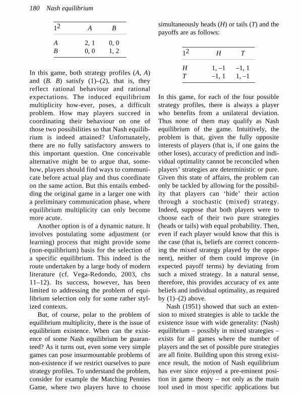
12 A B

A 2, 1 0, 0B 0, 0 1, 2

In this game, both strategy profiles (A, A)and (B. B) satisfy (1)–(2), that is, theyreflect rational behaviour and rationalexpectations. The induced equilibriummultiplicity how-ever, poses, a difficultproblem. How may players succeed incoordinating their behaviour on one ofthose two possibilities so that Nash equilib-rium is indeed attained? Unfortunately,there are no fully satisfactory answers tothis important question. One conceivablealternative might be to argue that, some-how, players should find ways to communi-cate before actual play and thus coordinateon the same action. But this entails embed-ding the original game in a larger one witha preliminary communication phase, whereequilibrium multiplicity can only becomemore acute.

Another option is of a dynamic nature. Itinvolves postulating some adjustment (orlearning) process that might provide some(non-equilibrium) basis for the selection ofa specific equilibrium. This indeed is theroute undertaken by a large body of modernliterature (cf. Vega-Redondo, 2003, chs11–12). Its success, however, has beenlimited to addressing the problem of equi-librium selection only for some rather styl-ized contexts.

But, of course, polar to the problem ofequilibrium multiplicity, there is the issue ofequilibrium existence. When can the exist-ence of some Nash equilibrium be guaran-teed? As it turns out, even some very simplegames can pose insurmountable problems ofnon-existence if we restrict ourselves to purestrategy profiles. To understand the problem,consider for example the Matching PenniesGame, where two players have to choose

simultaneously heads (H) or tails (T) and thepayoffs are as follows:

12 H T

H 1, –1 –1, 1T –1, 1 1, –1

In this game, for each of the four possiblestrategy profiles, there is always a playerwho benefits from a unilateral deviation.Thus none of them may qualify as Nashequilibrium of the game. Intuitively, theproblem is that, given the fully oppositeinterests of players (that is, if one gains theother loses), accuracy of prediction and indi-vidual optimality cannot be reconciled whenplayers’ strategies are deterministic or pure.Given this state of affairs, the problem canonly be tackled by allowing for the possibil-ity that players can ‘hide’ their actionthrough a stochastic (mixed) strategy.Indeed, suppose that both players were tochoose each of their two pure strategies(heads or tails) with equal probability. Then,even if each player would know that this isthe case (that is, beliefs are correct concern-ing the mixed strategy played by the oppo-nent), neither of them could improve (inexpected payoff terms) by deviating fromsuch a mixed strategy. In a natural sense,therefore, this provides accuracy of ex antebeliefs and individual optimality, as requiredby (1)–(2) above.

Nash (1951) showed that such an exten-sion to mixed strategies is able to tackle theexistence issue with wide generality: (Nash)equilibrium – possibly in mixed strategies –exists for all games where the number ofplayers and the set of possible pure strategiesare all finite. Building upon this strong exist-ence result, the notion of Nash equilibriumhas ever since enjoyed a pre-eminent posi-tion in game theory – not only as the maintool used in most specific applications but

180 Nash equilibrium

also as the benchmark concept guiding latertheoretical developments.

FERNANDO VEGA-REDONDO

BibliographyCournot, A. (1838), Recherches sur les Principes

Mathématiques de la Théoríe des Richesses, Paris:Hachette.

Nash, J. (1951), ‘Non-cooperative games’, Annals ofMathematics, 54, 286–95.

Vega-Redondo, F. (2003), Economics and the Theory ofGames, Cambridge, MA: Cambridge UniversityPress.

See also: Cournot’s oligopoly model.

Negishi’s stability without recontractingThis is named after Japanese economistTakashi Negishi (b.1933). A fundamentalproblem beyond the existence of a staticcompetitive general equilibrium consists ofestablishing a plausible dynamical mecha-nism whose equilibrium configurationcoincides with the static equilibrium solu-tion and enjoys some form of stability.Stability is a crucial dynamical propertyessentially implying that the whole statespace (global stability) or just a neighbour-hood of each equilibrium (local stability)asymptotically collapses to equilibria underthe action of the dynamics. This propertyhas important economic implications, suchas the fact that any set of initial observa-tions of the considered economic variableswill converge to market-clearing valuesunder the market dynamics. Furthermore,the equilibrium solution will remain robustunder perturbation, in accordance witheconomic facts.

The modern formulation (after Samuelson)of the Walrasian mechanics for adjustmentof the price system in a pure exchangecompetitive economy with n individualagents and m commodities is typically givenby the following system of differentialequations

dPj—— = Xj(P, X—) – X—j j = 1, 2, . . ., mdt

(1)dX—ij—— = Fij(P, X—) i = 1, 2, . . ., n, j = 1, 2, . . ., m,dt

where

• P(t) = (P1(t), P2(t), . . ., Pm(t)) is theprice vector of the economy;

• X —(t) = (X —ij(t))1≤i≤n,l≤j≤m is a matrixmonitoring the distribution of the stockof commodities among agents, so thatX—ij(t) represents the ith agent’s holdingof the jth good at time t;

• Xj(P, X—) = ∑ni=1Xij(P, X—i) renders the

aggregate demand for the jth commod-ity, the ith agent’s demand Xij for thejth good being obtained by maximizinga well-behaved utility function Ui(Xi1,Xi2, . . ., Xim) subject to the budgetconstraint ∑m

j=1PjXij = ∑mj=1PjX—ij;

• Fij are certain prescribed functions,aiming to represent the opportunitiesfor agents to exchange their holdings X—ij with each other.

Since there is no production, the totalamounts of each commodity remain con-stant, that is, X—j(t) ≡ ∑n

i=1X—ij(t) = X—j for all t,which in turn requires that ∑n

i=1Fij(P, X—) = 0for j = 1, 2, . . ., m.

The first set of evolution equations in (1)reflects the stylized fact that the marginalvariation of a commodity price and the corre-sponding excess demand have the same sign,whereas the equations of the second set spec-ify how the holdings of agents may evolve intime when exchanged according to theallowed trading rules.

An equilibrium of the system (1) is givenby a price vector P* and a distribution matrixX— * such that

Xj(P*, X—*) = X—*j for j = 1, 2, . . ., m.

Negishi’s stability without recontracting 181

The dynamical system (1) is globally stableif, for any solution (P(t), X—(t)),

(P(t), X—(t)) → (P*, X—*) as t →∞

for some equilibrium (P*, X—*). If the equilib-rium points are not isolated, but any solutionhas equilibrium as limit points, the system isnamed quasi-stable.

Under the assumption that no actual tradeis allowed at disequilibria, it holds that Fij =0, so that not only X—j but X— is a constantmatrix, and the model dynamics is steered bythe price equations in (1). Although no trans-action takes place until equilibrium isreached, recontracting may be permitted.This term refers to a mechanism of fictionaltrading through which agents renegotiatetheir demands after learning the pricesannounced by a market manager, in their turn sequentially computed from a deviceexpressed by (1). This important case corresponds with a so-called tâtonnementprice adjustment process embodied by theWalrasian auctioneer that manages recon-tracting.

In the non-recontracting case, holdingsamong agents vary according to theexchange laws defined in (1) and X— will notbe constant. In order to analyse non-recon-tracting stability, different specifications ofthe trading rules defined by the Fij may beconsidered (Negishi, 1962). Negishi (1961)deals with the general case of a barterexchange process, that is, even though thequantities X—ij may vary via trading, the totalvalue of the stock of commodities held byeach agent is not altered. This amounts to theFijs satisfying

m dX—ij m

∑Pj —— = ∑PjFij = 0 i = 1, 2, . . ., n.j=1 dt j=1

Negishi showed that any non-tâtonnementbarter exchange dynamics is quasi-stable in

the case that all commodities are (strict)gross substitutes. He also proved that globalstability holds under the further assumptionthat all the agents share the same strictlyquasi-concave and homogeneous utilityfunction. Proofs make essential use ofWalras’s law, that can be derived from therational behaviour of demanders under stan-dard assumptions.

JOSÉ MANUEL REY

BibliographyNegishi, T. (1961), ‘On the formation of prices’,

International Economic Review, 2, 122–6.Negishi, T. (1962), ‘The stability of a competitive econ-

omy: a survey article’, Econometrica, 30, 635–69.

See also: Hicksian perfect stability, Lyapunov stabil-ity, Marshall’s stability, Walras’s auctioneer.

von Neumann’s growth modelThe John von Neumann (1903–57) model,first published in 1932, is a multisectorialgrowth model; its crucial characteristics areconstant coefficients; alternative technol-ogies, without technical change; jointproduction; unlimited natural resources andlabour force availability.

Joint production makes it feasible to dealwith capital goods and depreciation in aspecial way. A capital good of age t is clas-sified as different from the same good withage (t + 1); this last capital good is the resultof a process using the first one in a jointproduction activity. Model variables are asfollows:

• qij is the stock of input i required tooperate process j at unit level;

• sij is the stock of i produced at the endof period (t + 1) when process j oper-ates at unit level;

• xj(t) is operational level of activity j,period t;

• pi(t) is price of product i at the begin-ning of time period t;

182 von Neumann’s growth model

• r(t) is rate of profit corresponding totime period t.

Workers consume a fixed vector. Capitalistare considered as non-consumers. Systemformalization is as follows. First, totaloutputs produced at the end of time period tmust be greater than or equal to inputs neces-sary for production at the end of time period(t + 1):

m m

∑sijxj(t) = ∑qijxj(t + 1).j=1 j=1

Secondly, capitalist competition impliesthat income processes cannot generate a rateof profit greater than the common rate ofprofit,

n n

[1 + r(t)]∑pi(t)qij ≥ ∑pi(t+1)sij.i=n i=1

To close the model we need to add someadditional constraints. A group refers to thenon-negativity of prices and levels of activ-ity. The rest of the constraints are known asthe ‘rule of profit’ and the ‘rule of freegoods’. The ‘rule of profit’ refers to everyactivity and excludes non-profit activities:

m m

[1 + r(t)]∑pi(t)qij ≥∑pi(t + 1)sij ⇒ xj(t + 1) ≡ 0.i=1 i=1

The rule of ‘free goods’ refers to everygood and classifies as free goods those withexcess supply,

m m

∑sijxj(t) ≥ ∑qijxj(t + 1) ⇒ pi(t) ≡ 0.j=1 j=1

The von Neumann stationary state verifies

p(t + 1) = p(t) = pr(t + 1) = r(t) = rx(t + 1) = x(t) = (1 + l) x(t),

where l is the equilibrated rate of growth,common to all sectors.

Price vectors and activity levels are semi-positive; total input and output values arepositive and the rate of profit equals the equi-librating rate of growth.

Morishima (1964) has formulated a rele-vant generalization of the model, considering(a) there is labour force finite growth; (b)workers are consumers, depending on wagesand prices; (c) capitalists are also consumers:they consume a constant proportion of theirincome and are sensitive to prices.

McKenzie (1967), among others, hascontributed to exploring the properties of themodel.

JOSEP MA. VEGARA-CARRIÓ

BibliographyMcKenzie, L.W. (1967), ‘Maximal paths in the von

Neumann model’, in E. Malinvaud and M.Bacharach (eds), Activity Analysis in the Theory ofGrowth and Planning, London: Macmillan Press,pp. 43–63.

Morishima, M. (1964), Equilibrium, Stability andGrowth, Oxford: Clarendon Press.

von Neumann, J. (1945–46), ‘A model of generaleconomic equilibrium’, Review of Economic Studies,13, 1–9.

von Neumann–Morgenstern expectedutility theoremModern economic theory relies fundamen-tally on the theory of choice. The currentfoundation for the use of utility functions as away to represent the preferences of so-calledrational individuals over alternatives thatconsist of bundles of goods in various quanti-ties is axiomatic. It is based on the proof that,if individual preferences (understood asbinary relations of the type ‘bundle x = a is atleast as good as bundle x = b’ on the set ofpossible bundles faced by the individual)satisfy some axioms (in particular those ofcompleteness, transitivity and continuity),then one can ensure the existence of a contin-uous utility function U(x) that represents

von Neumann–Morgenstern expected utility theorem 183

those preferences. That is, a function thatassigns a real number (or utility) to each ofthe relevant bundles x with the convenientproperty that, for the represented individual,a bundle a will be at least as good as anotherbundle b if, and only if, U(a) > U(b). Anobvious advantage of having such a functionis, for example, that the economic choices ofthe individual can be mathematically repre-sented as the result of maximizing such util-ity under the relevant set of constraintsimposed by the environment (for example, abudget constraint in the typical static modelof consumer theory).

When the alternatives faced by individ-uals are associated with uncertain outcomes,the theory of choice needs to be extended.The expected utility theorem of John vonNeumann (1903–57) and Oskar Morgenstern(1902–77) (1944, pp. 15–31) is the extensionthat, for more than half a century now, hasprovided economists (and other interestedscientists) with the most powerful tool for theanalysis of decisions under uncertainty.

The extension required, in the first place,having a way to represent the risky alterna-tives. Each risky alternative can be seen asleading to each of n possible outcomes (forexample, several bundles of goods, x1, x2, . . ., xn) with some probabilities p1, p2, . . . pn,respectively (for simplicity, the presentationwill focus on the choice among alternativesthat have a finite number (n) as possibleoutcomes, but the framework has a naturalextension for dealing with infinitely manypossible outcomes). A vector of probabilitiesover the possible outcomes, L = (p1, p2, . . .pn), is known as a ‘lottery’. Individual pref-erences over risky alternatives can then bethought of as a binary relationship of the type‘lottery L = a is at least as good as lottery L= b’ over the set of possible lotteries. Onsuch preferences one can impose, perhapsafter some technical adaptation, the samerationality and continuity axioms as in thestandard theory of choice under certainty.

The important contribution of vonNeumann and Morgenstern was, however, todiscover that, given the special structure oflotteries (which, contrary to the bundles ofgoods considered in the theory of choiceunder certainty, consist of probability distri-butions on mutually exclusive outcomes), itwas reasonable to add an extra axiom to thetheory: the ‘independence axiom’. In words,this axiom says that, if one makes a proba-bilistic mix between each of two lotteries anda third one, the preference ordering of thetwo resulting compound lotteries does notdepend on the particular third lottery used.Intuitively, and tracing a parallel with thetheory of choice between consumptionbundles, the independence axiom rules outthe existence of ‘complementarity’ betweenthe lotteries that form a compound lottery.Imposing the absence of complementarity inthis context is natural since each of the lot-teries in a probabilistic mix cannot be‘consumed’ together but, rather, one insteadof the other.

Under the independence axiom, individ-ual preferences over lotteries allow the‘expected utility representation’. In essence,one can prove that there exists an assignmentof so-called von Neumann–Morgenstern utili-ties ui to each of the i = 1, 2, . . ., n possiblelottery outcomes, such that the utility of anylottery L can be computed as the expectedutility U(L) = p1u1 + p2u2, + . . . + pnun (seeMas-Colell et al. (1995, pp. 175–8) for amodern and didactic proof). The reason whyU(L) is referred to as the expected utility oflottery L is obvious: it yields an average ofthe utilities of the various possible outcomesof the lottery weighted by the probabilitieswith which they occur under the correspond-ing lottery.

The expected utility theorem has beenvery useful for the development of the theoryof choice under uncertainty and its importantapplications in modern micro, macro andfinance theory. However, the key hypotheses

184 von Neumann–Morgenstern expected utility theorem

of the theorem, especially the independenceaxiom, have been criticized from variousfronts. Constructed examples of choicebetween simple lotteries, such as the Allaisparadox, show that individuals may fre-quently behave in a way inconsistent with thehypotheses. Machina (1987) contains a goodreview of this and related criticisms and thetheoretical reaction to them.

JAVIER SUÁREZ

BibliographyMachina, M. (1987), ‘Choice under uncertainty: prob-

lems solved and unsolved’, Journal of EconomicPerspectives, 1 (1), 121–54.

Mas-Colell, A., M. Whinston and J. Green (1995),Microeconomic Theory, New York: OxfordUniversity Press.

von Neumann, J. and O. Morgenstern (1944), Theory ofGames and Economic Behavior, Princeton, NJ:Princeton University Press.

See also: Allais paradox, Ellsberg paradox, Friedman–Savage hypothesis.

von Neumann–Morgenstern stable setA game in characteristic function form is apair (N, v), where N is the non-empty set ofplayers and v is the characteristic functiondefined on the family of subsets of N suchthat v(∅ ) = 0. A non-empty subset of N iscalled ‘coalition’ and v(S) is interpreted asthe worth of coalition S.

An imputation is any ntuple x of realnumbers satisfying xi ≥ v({i}) for all i∈ N and∑i∈ Nxi = v(N). An imputation y = (y1, . . ., yn)dominates an imputation x = (x1, . . ., xn) withrespect to a non-empty coalition S if thefollowing two conditions are satisfied:∑i∈ Nyi ≤ v(S), and yi > xi for all i∈ S.

The first condition admits imputation y asdominating imputation x only if y is feasiblein the sense that players in S can guaranteethemselves the amount prescribed by y. Thesecond condition implies that every player inS strictly prefers y to x.

A stable set of a game (N, v) is defined tobe a set of imputations A such that

• no y contained in A is dominated by anx contained in S (internal stability);

• every y not contained in A is dominatedby some x contained in A (externalstability).

John von Neumann (1903–57) and OskarMorgenstern (1902–77) consider a stable setas a characterization of what may be accept-able as a standard of behavior in society.Thus internal stability expresses the fact thatthe standard of behavior has an inner consist-ency. It guarantees the absence of innercontradictions. External stability gives areason to correct deviant behavior that is notconformable to the acceptable standard ofbehavior.

As an extension of this concept, vonNeumann and Morgenstern provide in theirbook (65.2.1) the basis for a more generaltheory in the sense that, instead of imputa-tions, they consider an arbitrary set D and anarbitrary relation defined on D.

ELENA IÑARRA

Bibliographyvon Neumann, J. and O. Morgenstern, (1944), Theory of

Games and Economic Behavior, Princeton, NJ:Princeton University Press.

Newton–Raphson methodThis method computes zeros of nonlinearfunctions through an iterative procedure thatconstructs the best local linear approxima-tion to the function and takes the zero of theapproximation as the next estimate for thezero of the function. The method can beeasily extended to the computation of solu-tions for systems of nonlinear equations ofthe form F(x) = 0. In this case, it starts withan initial estimate of the solution x0, andimproves it by computing xk+1 = xk – ∇ F(xk)

–1F(xk).The procedure is guaranteed to obtain a

solution x* with arbitrary precision as long as

Newton–Raphson method 185

the initial estimate x0 is close enough to thissolution and the Jacobian ∇ F(x*) is non-singular.

The main application of the method andits variants is the computation of local solu-tions for unconstrained or constrained opti-mization problems. These problems arise inmultiple contexts in economic theory andbusiness applications. In these cases, themethod is applied to the computation of asolution for a system of equations associatedwith the first-order optimality conditions forsuch problems.

The method derives its name from JosephRaphson (1648–1715) and Sir Isaac Newton(1643–1727). Raphson proposed the methodfor the computation of the zeros of equationsthat shares his name in a book (Analysisaequationum universalis) published in 1690,while Newton described the same method aspart of his book Methodis Serierum etFluxionem, written in 1671, but not pub-lished until 1736.

F. JAVIER PRIETO

BibliographyNewton, I. (1736), Methodis Serierum et Fluxionem.Raphson, J. (1690), Analysis aequationum universalis.

Neyman–Fisher theoremAlso known as the ‘Neyman–Fisher factor-ization criterion’, this provides a relativelysimple procedure either to obtain sufficientstatistics or to check whether a specificstatistic could be sufficient.

Fisher was the first to establish the factor-ization criterion as a sufficient condition forsufficient statistics in 1922. Years later, in1935, Neyman demonstrated its necessityunder certain restrictive conditions. Finally,Halmos and Savage extended it in 1949 asfollows:

Let ℘ = {Pq, q∈ W} be a family of probabilitymeasures on a measurable space (QX, A)absolutely continuous with respect to a s-finite

measure m. Let us suppose that its probabilitydensities in the Radon–Nicodym sense pq =dPq/dm exist a.s. [m] (almost sure for m).

A necessary and sufficient condition for thesufficiency with respect to ℘ of a statistic Ttransforming the probability space (QX, A, Pq)into (QT, B, PT) is the existence ∀ q∈ W of aT–1(B)-measurable function gqT(x) and an A-measurable function h(x) ≠ 0 a.s. [Pq], bothdefined ∀ x∈ Qx, non-negatives and m-inte-grable, such that pq(x) = gqT(x) · h(x), a.s. [m].

Densities pq can be either probabilitydensity functions from absolutely continuousrandom variables or probability functionsfrom discrete random variables, among otherpossibilities, depending on the nature anddefinition of m.

In common economic practice, this factor-ization criterion adopts simpler appearances.Thereby, in estimation theory under randomsampling, the criterion is usually enouncedas follows:

Let X be a random variable belonging to aregular family of distributions F(x; q) whichdepends on a parameter q (mixture ofabsolutely continuous and discrete randomvariables on values not depending on the para-meter) representing some characteristic ofcertain population. Moreover, let x = (X1, X2, . . ., Xn) represent a random sample size n of X,extracted from such a population.

A necessary and sufficient condition for thesufficiency of a statistic T = t(x) with respect tothe family of distributions F(x; q) is that thesample likelihood function Ln(x; q) could befactorized like Ln(x; q) = g(T; q) · h(x). Here‘g’ and ‘h’ are non-negative real functions, ‘g’depending on sample observations through thestatistic exclusively and ‘h’ not depending onthe parameter.

When the random variable is absolutelycontinuous (discrete), function g(t; q) isclosely related to the probability densityfunction (probability function) of the statisticT. Thus the criterion could be equivalentlyenounced assuming the function g(t; q) to beexactly such probability density function

186 Neyman–Fisher theorem

(probability function). In this case, theusually complex work of deducing the distri-bution x | T of the original observationsconditioned to the statistic T becomes easier,being specified by h(x). According to thisfactorization criterion, any invertible func-tion of a sufficient statistic T* = k(T) is asufficient statistic too.

Likewise, an exponential family definedby probability density functions such as f(x;q) = k(x) · p(q) · exp[c(q)′T(x)] always admitsa sufficient statistic T.

FRANCISCO J. CALLEALTA

BibliographyFisher, R.A. (1922), ‘On the mathematical foundation of

theoretical statistics’, Philos. Trans. Roy. Soc.,Series A, 222, 309–68.

Halmos, P.R. and L.J. Savage (1949) ‘Application of theRadon–Nikodym theorem to the theory of sufficientstatistics’, Ann. Math. Statist., 20, 225–41.

Neyman, J. (1935), ‘Sur un teorema concernente lecosidette statistiche sufficienti’, Giorn. Ist. Ital. Att.,6, 320–34.

Neyman–Pearson testThis is a framework for hypothesis testingthat differed considerably from Fisher’s,giving rise to some controversy. Nowadays,it is the basis of modern hypothesis testing.

Egon S. Pearson (1895–1980), son of KarlPearson, was born in England. He joined hisfather’s department at University College,London. When his father resigned, heassumed one of the two positions created asreplacements, the second position being forR.A. Fisher. Jerzy Neyman (1894–1981) wasborn in Russia. He went to England to workwith Karl Pearson and then started to workwith E.S. Pearson, on a general principle forhypothesis testing.

Testing a null hypothesis was introducedby Fisher as a procedure to form an opinionabout some parameter. A limitation inFisher’s formulation is that for each nullhypothesis one could construct several teststatistics, without providing a way to choose

the most appropriate. Conversely, Neymanand Pearson (1928) viewed hypothesis test-ing as a means to decide between twooptions: the null hypothesis (H0) and thealternative hypothesis (H1), while at thesame time controlling the chances of errors.The Neyman–Pearson specification of bothhypotheses is H0:q∈ W0, against H1:q∈ W1,W0∩W1 = 0. The two errors here are rejectingH0 if it is true (type I error), and accepting itwhen it is false (type II error). Through thedesign of the test it is possible to control theprobability of each error. There is, however,a trade-off between them.

Given a test statistic d(x), we reject H0when | d(x) | > c (for some constant c). Theprobability of type I error is, then, P(| d(x) |> c); H0 true) = a and it is often called the size of the test. In the Neyman–Pearsontest, H0 is more important than H1.Consequently, the analyst should choose asmall a. Given a, the analyst chooses the teststatistic that minimizes the type II error.Neyman and Pearson (1933) solve the prob-lem of obtaining a statistical test in order toobtain an optimal test (minimizing type IIerror). The limitation however, is, that theyprovide optimal tests only in one simplecase. Let f(x; q) denote the distribution of thesample (density function or mass function).Let us consider testing H0: q = q0 against H1:q = q1, using a test with rejection region Rdefined as

x∈ R if f(x; q1) > kf(x; q0), (1a)

x∈ Rc if f(x; q1) ≤ kf(x; q0), (1b)

for some k ≥ 0 and P(X∈ R | q = q0) = a.Then, by the Neyman–Pearson lemma, sucha test is an optimal test of size a. Also, ifthere exists a test satisfying (1), then everyoptimal test of size a coincides with (1).Hence, should an optimal test exist, it is afunction of f(x, q1)/f(x; q0). The specific formof such a function can be a complex problem

Neyman–Pearson test 187

that needs to be solved in each situation.There have been some extensions of thislemma that makes it possible to build nearlyoptimal tests in more complex problems.

ISMAEL SÁNCHEZ

BibliographyNeyman, J. and E.S. Pearson (1928), ‘On the use and

interpretation of certain test criteria for purposes ofstatistical inference, part I’, Biometrika, 20, 175–240.

Neyman, J. and E.S. Pearson (1933), ‘On the problem ofthe most efficient tests of statistical hypothesis’,Philosophical Transactions of the Royal Society, A,231, 289–337.

188 Neyman–Pearson test

Occam’s razorThis is a logical principle named after the medieval Franciscan friar–philosopherWilliam of Occam (1285?–1349?), statingthat the number of entities required toexplain anything should not be increasedunnecessarily. This principle is also calledthe law of economy, parsimony or simplicity.It is usually interpreted as ‘the simpler theexplanation, the better’. Sometimes it isquoted in one of its original Latin forms,‘pluralitas non est ponenda sine necessitate’,‘frustra fit per plura quod potest fieri perpauciora’ or ‘entia non sunt multiplicandapraeter necessitatem’. A basic scientific prin-ciple, it can heuristically distinguish theoriesthat make the same predictions, and indicatewhich to test first, but does not guarantee thefinding of a correct answer.

VICTORIANO MARTÍN MARTÍN

BibliographyOccam, W. (1324), Quodlibetal Questions, Quodlibeta

no. 5, 9,1, art. 2.Thorburn, W.M. (1918), ‘The myth of Occam’s razor’,

Mind, 27, 345–53.

Okun’s law and gapOkun’s law is the empirical regularitybetween unemployment rate and GNP firstestimated by Arthur M. Okun (1928–80),Chairman of the Council of EconomicAdvisers in the 1960s.

According to Okun, ‘in the postwar period[and in the US economy], on average, eachextra percentage point in the unemploymentrate above four per cent has been associatedwith about a three per cent decrement in realGNP’ (Okun, 1983, pp. 146, 148). Almosttwo decades after the result was firstpublished (in 1962), Okun wrote:

Nearly twenty years ago, I found in the data ofthe fifties an approximate rule of thumb that anincrease of one percentage point in unemploy-ment was associated with a decrement of aboutthree percentage points in real GNP. The ruleof thumb held up so well over the next decadethat some of my professional colleaguesnamed it ‘Okun’s Law’. (Okun, 1981, p. 228).

In J. Tobin’s words, it became ‘one of themost reliable empirical regularities of macro-economics’ (Tobin, 1987, p. 700). The resultwas arrived at after implementing threestatistical methods, thereby giving rise tothree versions of the ‘law’.

First differences (growth) versionUsing quarterly observations from 1947 to1960, Okun estimated the following linearregression

DUt = 0.30 – 0.30gt,

where DUt denotes the change in unemploy-ment rate and gt the growth rate of real GNP(both Ut and gt measured in percentagepoints). Therefore, ‘for each extra one percent of GNP, unemployment is 0.3 pointslower’ (Okun, 1983, p. 148). Assuming (asOkun did) that the previous estimation couldbe inverted, one would obtain the more usualtextbook way in which the growth version ofthe law is expressed,

gt = 1 – 3.3DUt,

so that ‘one percentage more in the unem-ployment rate means 3.3 per cent less GNP’(ibid.).

Concerning the intercept of the equation,a constant unemployment rate is associatedwith a positive (full employment) output

189

O

growth rate because of (a) gains in labourproductivity (due to technological progressand to physical and human capital accumula-tion), and (b) growth in the labour force. Asfor the slope, several factors explain whyreductions in the unemployment rate shouldinduce higher proportional increments in theoutput growth rate around its trend (or whythe estimated coefficient of DUt should begreater than one). Higher participation ratesdue to less discouraged workers; increasednumber of hours per worker (not necessarilyin the same job); lower on-the-job unem-ployment (labour hoarding); and more inten-sive use of plant and equipment.

Trial gaps (level) versionAlternatively, using quarterly observationsfrom 1953 to 1960, Okun estimated also thefollowing regression:

Ut = 3.72 + 0.36gapt,

where Ut stands for unemployment rate andgapt is the (estimated) GNP gap (both inpercentage points), where the potential GNPwas ‘derived from a 3.5 per cent trend linethrough actual real GNP in mid-1955’(Okun, 1983, p. 149). Assuming once againthat the estimation could be inverted, oneobtains

gapt = 2.8 (Ut – 3.72).

Therefore ‘an increment of unemploy-ment of one per cent is associated with anoutput loss equal to 2.8 per cent of potentialoutput (. . .). The estimated unemploymentrate associated with a zero gap is 3.72 percent, not too far from the 4.0 per cent ideal’Okun claimed as a principle that ‘potentialGNP should equal actual GNP when U = 4’,and textbooks usually refer to this rate as thenatural rate of unemployment when explain-ing Okun’s law (ibid. p. 149). This versionof Okun’s result stresses its economic

policy- oriented relevance: ‘Focus on the“gap” helps to remind policymakers of thelarge reward [in terms of increased produc-tion] associated with such an improvement[the reduction of the unemployment rate]’(ibid., p. 146). Had other factors beencontrolled for in the regression, the effect ofunemployment would of course have beensubstantially reduced (Prachowny, 1993,Freeman, 2001).

Fitted trend and elasticity versionFinally, in a less cited version, Okunconfirmed his rule of thumb without assum-ing a trend for the potential output but ratherestimating it, claiming that ‘each onepercentage point reduction in unemploymentmeans slightly less than 3 per cent incrementin output (near the potential level)’ (Okun,1983, p. 150).

Is the three-to-one ratio a true ‘law’, validat any time and everywhere? Clearly not. AsOkun himself admitted, ‘During the lateseventies, the three-to-one ratio no longerapproximated reality’ (Okun, 1981, p. 228).Considering, for instance, the growth versionof the law for different countries, twopatterns for the coefficient (in absolutevalue) of gt clearly show up. First, it differsacross economies: countries whose firmsoffer their workers a high level of job stab-ility and where labour market rigidities arestronger usually display lower coefficients.And, second, it has increased over time.Several reasons are pointed out for structuralbreaks in the dynamics of output and unem-ployment: augmented international competi-tion among world economies has forcedfirms to be less committed to job stability,fewer legal restrictions on hiring and firinghave reduced turnover costs and labourhoarding by firms, and increased femaleparticipation implies higher competitionamong workers.

CRUZ ANGEL ECHEVARRÍA

190 Okun’s law and gap

BibliographyFreeman, D.G. (2001), ‘Panel tests of Okun’s law for ten

industrial economies’, Economic Inquiry, 39 (4),511–23.

Okun, A.M. (1981), Prices and Quantities: A Macro-economic Analysis, Washington, DC: TheBrookings Institution.

Okun, A.M. (1983), ‘Potential GNP: its measurementand significance’, in Joseph A. Pechman (ed.),

Economics for Policy Making, Selected Essays ofArthur M. Okun, Cambridge, MA: MIT Press, pp.145–58; article first published (1962) in Proceedingsof the Business and Economic Statistics Section,American Statistical Association, Washington:ASA, 98–103.

Prachowny, M.F.J. (1993), ‘Okun’s law: theoreticalfoundations and revised estimates’, The Review ofEconomics and Statistics, 75 (2), 331–6.

Okun’s law and gap 191

Paasche indexThe Paasche price index, Pp, is a weightedaggregate index proposed by German economist H. Paasche (1851–1925),defined as

n

∑pitqiti=1

Pp = ———,n

∑pi0qiti=1

where pit is the price of commodity i (i = 1, . . ., n) in period t, qit is the quantity of sucha commodity in that period, and pi0 is theprice of commodity i in period 0 (the baseyear). The numerator of Pp shows the costof a basket of goods purchased in the year tat prices of that year, whereas the denomi-nator displays the cost of the same basketof goods at the base year prices. As in thecase of the Laspeyres index, Pp allowscomputing the rate of variation of the valueof a basket of goods, with the differencethat the Paasche index uses the currentquantities as weights (qit). Therefore, as theweights vary through time, Pp is not anaccurate index to use on a continuing basis(it is not used, for example, for theconstruction of the consumer price index,because it would need to carry out a perma-nent consumption survey). Moreover, Pptends to underestimate the effect of a priceincrease, because it uses the current yearquantities as weights, which are likely to besmaller than in the base year when pricesincrease.

If prices are used as weights instead ofquantities, it is possible to compute thePaasche quantity index, Pq, defined as

n

∑qitpiti=1

Pq = ———,n

∑qi0piti=1

This index is used in the consumer theory tofind out whether the individual welfareincreases from period 0 to period t. If Pq isgreater than 1, it is possible to state that theconsumer welfare is greater at the currentyear than in the base year.

CÉSAR RODRÍGUEZ-GUTIÉRREZ

BibliographyAllen, R.G.D. (1975), Index Numbers in Theory and

Practice, Chicago: Aldine Publishing Company.

See also: Divisia index, Laspeyres index.

Palgrave’s dictionariesThe Dictionary of Political Economy, editedby Sir R.H. Inglis Palgrave (1827–1919), aone-time banker, author of different writingson aspects of banking practice and theory,and editor of The Economist, appeared inthree volumes in 1894, 1896 and 1899. Thesewere reprinted, with corrections and addi-tions, during the first two decades of thetwentieth century. A new edition by H. Higgswas published between 1923 and 1926 underthe title Palgrave’s Dictionary of PoliticalEconomy. The primary object of this was ‘toprovide the student with such assistance asmay enable him to understand the position ofeconomic thought at the present time and topursue such branches of inquiry as may benecessary for that end’.

These goals were reasonably well

192

P

fulfilled. Palgrave was fortunate in beingable to enlist the support of importantscholars, such as W.J. Ashley, E. Cannan,F.Y. Edgeworth, J.K. Ingram, J.N. Keynes,M. Pantaleoni, H.R. Tedder and H.Sidgwick. Edgeworth’s 126 entries wereenough to confer distinction on theDictionary. Six decades later, it was editedas The New Palgrave: A Dictionary ofEconomics. Launched in 1982, with all fourvolumes available by 1987, it containsapproximately 2000 articles, written bymore than 900 contributors; 50 entries fromthe original Palgrave were reprinted here(these were selected to emphasize thecontinuity between the ‘old’ Palgrave andthe ‘new’).

Both the great increase in its size and thefact that it required three editors (J.Eatwell, M. Milgate and P. Newman) areevidence of the vitality of economics in thetwentieth century. The New Palgraveattempts to define the state of the disciplineby presenting a comprehensive and criticalaccount of economic thought. Like itspredecessor, it strives to place economictheory in historical perspective. It includesover 700 biographical entries – even someon living economists aged 70 or more in1986. Most articles are followed by a usefulbibliography.

Despite its broad scope, some of theeditors’s choices have been questioned: TheNew Palgrave virtually excludes empiricalmaterial; the mathematical aspects of moderneconomics do not receive sufficient attentionand neither do institutional and policy issues;finally, it is strongly oriented to the pre-sentation of Sraffian, Marxian and Post-Keynesian doctrine. Nevertheless, it is anunquestionably authoritative reference workon economic theory and the work of thoseeconomists who contributed to its develop-ment.

JESÚS ASTIGARRAGA

BibliographyMilgate, M. (1987), ‘Palgrave, Robert Harry Inglis

(1827–1919)’, ‘Palgrave’s Dictionary of PoliticalEconomy’, in J. Eatwell, M. Milgate and P. Newman(eds), The New Palgrave: A Dictionary ofEconomics, vol. III, London: Macmillan, pp.789–92.

Milgate, M. (1992), ‘Reviewing the reviews of the NewPalgrave’, Revue Européenne des Sciences Sociales,30 (92), 279–312.

Stigler, G.J. (1988), ‘Palgrave’s Dictionary ofEconomics’, Journal of Economic Literature, 26 (4),1729–36.

Palmer’s ruleThis empirical rule was adopted in 1827 andformulated in 1832 in a memorandum byG.W. Norman, of the Board of Directors ofthe Bank of England, with margin notes byJohn Horsley Palmer, governor of the bank.It established that, in normal times, the bankhad to keep reserves of currency andprecious metals equivalent to a third of itsliabilities (total deposits and notes issued),with the other two-thirds in governmentsecurities and other interest-yielding assets.Once this portfolio had been established, thebank’s active transactions (discounts, loansand investments) had to be kept approxi-mately constant, so that changes in currencycirculation would be due to gold entering orleaving the country. In this way, the circula-tion would behave as if it were metallic. Therule, on some occasions broken, was in linewith the theories of the currency school aspart of its debate during the first half of thenineteenth century with the banking school,providing the ideal basis for a permanentcurrency policy for the central bank.According to Schumpeter, it anticipates theprinciple of Peel’s law (1844) and might beadopted pending some regulation of thistype.

ANTÓN COSTAS

BibliographyHorsefield, J.K. (1949), ‘The opinions of Horsley

Palmer’, Economica, 16 (62), May, 143–58;

Palmer’s rule 193

reprinted in T.S. Ashton and R.S. Sayers, (eds)(1953), Papers in English Monetary History,Oxford: Clarendon Press, pp. 126–31.

Viner, J. (1937), Studies in the Theory of InternationalTrade, New York: Harper & Brothers.

See also: Peel’s law.

Pareto distributionThis is a power law distribution coined afterthe Italian economist Vilfredo Pareto (1848–1923) in 1897. He questioned the proportionof people having an income greater than agiven quantity x and discovered that this wasproportional to an inverse power of x. If Pdenotes the probability or theoretical propor-tion and X the income or any other randomvariable following a Pareto law, the formalexpression for the answer, in terms of thecumulative distribution function is P(X > x) =(k/x)a for X > k. The value k is the minimumvalue allowed for the random variable X,while the (positive) parameter a is the powerlaw slope. If a is less than one, there is nofinite mean for the distribution. If it is lessthan two, there is no finite variance, and soon. In general, the tails in this distribution arefatter than under the normal distribution. Aninteresting property is that the distribution is‘scale-free’, which means that the proportionof small to large events is always the same,no matter what range of x one looks at. Thisis very useful for modelling the size ofclaims in reinsurance.

EVA FERREIRA

BibliographyPareto, Vilfredo (1897), Cours d’Economie Politique,

Lausanne: Rouge.

Pareto efficiencyModern welfare economics is based on thenotion of efficiency (or optimality) proposedby Vilfredo Pareto (1909). To give a formaldefinition, consider an exchange economy

with m consumers and n goods, where eachconsumer i is characterized by a consump-tion set Xi ⊂ Rn, preferences over consump-tion bundles described by a utility functionui: Xi → R, and an initial endowment ei ∈ Rn.An allocation is an m-tuple x = (x1, . . ., xm)such that xi ∈ Xi for all i, and

∑mi=1xi = ∑m

i=1ei.

In words, an allocation is a distribution of the economy’s aggregate endowmentamong the consumers such that the bundlecorresponding to each consumer belongs toher consumption set. An allocation x is saidto be Pareto-efficient if there is no alloca-tion x� = (x �1, . . ., x �m) such that ui(x �i) ≥ui(xi) for all i and ui(x �i) > ui(xi) for some i,that is, if it is impossible to make anyconsumer strictly better off without makingsome other consumer worse off. It is impor-tant to realize that, in general, there areinfinitely many Pareto-efficient allocations,so it is a weak notion of efficiency.Moreover, it is a notion that ignores distri-butional issues that require interpersonalcomparisons of utilities. Thus extremelyunequal allocations may be Pareto-effi-cient.

The key insight of Pareto (1909, mathe-matical appendix) was to link his notion ofefficiency with the properties of competi-tive equilibrium allocations. A competitiveequilibrium is a pair (p, x) where p ∈ Rn isa price vector and x is an allocation suchthat, for all i, xi maximizes ui(xi) subject tothe budget constraint p · xi ≤ p · ei. The firstwelfare theorem states that, if (p, x) is acompetitive equilibrium, then under veryweak assumptions x is Pareto-efficient. Thisresult formalizes the intuition of AdamSmith that a set of individuals pursuing theirown interests through competitive marketsleads to an efficient allocation of resources.The second welfare theorem states that, if xis a Pareto-efficient allocation, then under

194 Pareto distribution

somewhat stronger assumptions there existsa price vector p such that (p, x) is a compet-itive equilibrium for a suitable redistribu-tion of the initial endowments. This resultshows how competitive markets may beused to decentralize any Pareto-efficientallocation.

Somewhat surprisingly, the proof of thefirst welfare theorem is almost trivial.Suppose, on the contrary, that there exists anallocation x� such that ui(x �i) ≥ ui(xi) for all i,and ui(x�i) > ui(xi) for some i. Then the defi-nition of competitive equilibrium (togetherwith a very weak assumption on preferenceslike local non-satiation) implies that p · x�i ≥p · ei for all i, with strict inequality for somei, so

p · ∑mi=1x�i > p · ∑m

i=1ei,

contradicting the assumption that

∑mi=1x�i = ∑m

i=1ei.

The notion of Pareto efficiency as well asthe welfare theorems can be easily extendedto economies with production. They can alsobe extended to economies with uncertainty,although this requires the existence of acomplete set of contingent markets. Withincomplete markets, competitive equilibriumallocations are not in general Pareto-effi-cient, although in certain special cases theycan be shown to be ‘constrained Pareto-effi-cient’, that is efficient relative to the set ofavailable markets. For a thorough discussionof these issues, as well as complete proofs ofthe welfare theorems, see Mas-Colell et al.(1995, chs 16, 19).

The notion of Pareto efficiency is alsoused outside the field of competitive equilib-rium analysis. For example, in cooperativegame theory it is one of the assumptions thatcharacterize the Shapley value, in coopera-tive bargaining theory it is one of the axiomsused to derive the Nash bargaining solution,

and in social choice theory it is one of theassumptions in the proof of Arrow’s impos-sibility theorem.

RAFAEL REPULLO

BibliographyMas-Colell, A., M.D. Whinston and J.R. Green (1995),

Microeconomic Theory, Oxford: Oxford UniversityPress.

Pareto, V. (1909), Manuel d’Économie Politique, Paris:Giard et Brière.

See also: Adam Smith’s invisible hand, Arrow’simpossibility theorem, Arrow–Debreu general equi-librium model, Nash bargaining solution, Shapleyvalue.

Pasinetti’s paradoxAs is well known, the factor–price curve (w– r) has a negative slope. When we considerseveral w – r curves generated by differenttechniques, nothing excludes multiple inter-sections, with the possibility of return oftechniques; as a matter of fact, it is easy tobuild numerical examples. This fact hasanalytical implications that we will analysebriefly.

We will use the factor–price curve (Figure1) as the tool for analysis. Formula (1) refersto one specific linear technique and can befocused in terms of k, the intensity of capital;k is ABC tangent:

q = rk + wk = (q – w)/r (1)

Consider now two techniques, a and b(Figure 2); technique a corresponds to thestraight line. Technique a is used when r issmall; at the transition point from techniquea to b, k decreases. If r increases, the tech-nique used is b and, as can be seen, kincreases. If r rises, technique a is againused and at the transition point from tech-nique a to b, k increases: A is a reswitchingpoint.

Pasinetti’s paradox 195

196 Pasinetti’s paradox

r

B

w

A

C

Pasinetti’s paradox, technique a

r

w

A

a

a

b

Pasinetti’s paradox, technique b

This simple analysis has relevant conse-quences:

• reswitching destroys the view of amonotonous order of techniques, interms of k;

• reduction of r does not necessarilyincrease capital intensity;

• the rate of profit is not a capital scarcityindicator.

These are the main reasons for the centralrole reswitching has played in the so-called‘Cambridge controversy on capital’ (see L.L.Pasinetti, P.A. Samuelson and R.M. Solow,among others).

JOSEP MA. VEGARA-CARRIÓ

BibliographyBurmeister, E. (1980), Capital Theory and Dynamics,

Cambridge: Cambridge University Press.Samuelson, P.A. and F. Modigliani (1966), ‘The

Pasinetti paradox in neoclassical and more generalmodels’, Review of Economic Studies, 33 (4),269–301.

Patman effectIncreasing interest rates fuel inflation. Namedafter American lawyer and congressmanWright Patman (1893–1976), a scathing criticof the economic policies of President HerbertHoover and Secretary of the Treasury AndrewMellon, the term was coined or at least usedby James Tobin (1980, p. 35) in his discus-sion of stabilization and interest costs.Driskill and Shiffrin (1985) said that undercertain circumstances the interest rate effecton price levels may be a matter of macroeco-nomic concern, although their model ‘doesnot support Patman’s view that it is senselessto fight inflation by raising interest rates’(ibid., 160–61). Seelig (1974) concluded thatonly if interest rates had been double theiraverage values in the period 1959–69 wouldthey have become an important determinantof prices. Driskill and Shiffrin add:

Monetary economists have always had anuneasy relationship with the populist view,associated with the late Congressman WrightPatman, that high interest rates ‘cause’ infla-tion. While interest rates are indeed a cost ofdoing business and may affect price determi-nation, the traditional position of monetaryeconomists is that restrictive monetary policywill, in the long run, reduce both inflation andinterest rates. (1985, 149)

Myatt and Young (1986) pointed out thatmacroeconomics models focused on aggre-gate demand of the 1950s or 1960s wereunable to assess the Patman effect, and thatthe theoretical studies of the aggregatesupply, after the OPEC oil prices shocks,had come to reveal other ways in whichhigh interest rates may have inflationaryeffects. They conclude: ‘There is noevidence of a Patman effect in the recent eraof the US economy. There is evidence,however, of inflation having a strong causalinfluence on both nominal and real interestrates’ (113).

ROGELIO FERNÁNDEZ DELGADO

BibliographyDriskill, R.A. and S.M. Sheffrin (1985), ‘The “Patman

effect” and stabilization policy’, Quarterly Journalof Economics, 100 (1), 149–63.

Myatt A. and G. Young (1986), ‘Interest rates and infla-tion: uncertainty cushions, threshold and “Patman”effects’, Eastern Economic Journal, 12 (2), 103–14.

Seelig, Steven (1974), ‘Rising interest rates and costpush inflation’, Journal of Finance, 29 (4), 1049–61.

Tobin, James (1980), ‘Stabilization policy ten yearsafter’, Brookings Papers on Economic Activity, 1,19–89.

Peacock–Wiseman’s displacement effectThese two British authors, Alan TurnerPeacock (b.1922) and Jack Wiseman (b.1919),observed that public expenditure increased inthe UK between 1890 and 1955. However, itdid not rise at a more or less regular rate, butshowed a series of plateaux and peaks, whichseemed to be associated with periods of war orof preparation for war.

Peacock–Wiseman’s displacement effect 197

On the basis of these data, they formu-lated their ‘displacement effect’ hypothesis:

1. Governments try to increase publicexpenditure but they cannot go furtherthan the burden of taxation consideredtolerable by their citizens.

2. From time to time, there are some majorsocial disturbances, such as warfare.During the periods when citizens acceptadditional tax increases, their highertolerance explains the peaks and the so-called ‘displacement effect’.

Once the disturbance is over, citizens willprobably continue to tolerate a higher taxburden, allowing in this way for publicexpenditure in new services. Therefore eachplateau after a peak will be higher than theprevious one. Peacock and Wiseman call thissecond step the ‘inspection effect’. Theyadmit, nevertheless, that this hypothesis doesnot explain the growth of public expenditurein all countries and at all times, and also thatchanges in public expenditure can be influ-enced by a number of different factors.

Many authors have included the ‘displace-ment effect’ in a secular rising tendency ofthe share of the public expenditure withsporadic upward shifts of the trend line.

JUAN A. GIMENO

BibliographyHenrekson, M. (1993), ‘The Peacock–Wiseman hypoth-

esis’, in N. Gemmel (ed.), The Growth of the PublicSector, Aldershot, UK and Brookfield, US: EdwardElgar, pp. 53–71.

Peacock, A. and J. Wiseman (1961), The Growth ofPublic Expenditure in the United Kingdom,Princeton, NJ: Princeton University Press.

See also: Wagner’s law.

Pearson chi-squared statisticsLet Y1, Y2, . . ., Yn be a random sample of sizen with discrete realizations in c = {1, 2, . . .,

k} and iid. according to a probability distribu-tion p(q); q∈ Q. This distribution is assumedto be unknown, but belonging to a knownfamily,

P = {p(q) ≡ (p1(q), . . ., pk(q)): q ∈ Q},

of distribution on c with Q⊂ Rt(t < k – 1). Inother words, the true value of the parameterq = (q1, . . ., qt) ∈ Q is assumed to beunknown. We denote p = (p 1, . . ., pk) with

Xjpj = —,

n

where Xj is the number of data taking thevalue j; j = 1, . . ., k.

The statistic (X1, . . ., Xk) is obviouslysufficient for the statistical model underconsideration and is multinomial distributed;that is, for q∈ Q,

Pr(X1 = x1, . . ., Xk = xk)n!

= ———— p1(q)x1 × . . . × pk(q)xk (1)x1! . . . xk!

for integers x1, . . ., xk ≥ 0 such that x1+ . . . +xk = n.

To test the simple null hypothesis,

H0: p = p(q0), (2)

where q0 is prespecified, the Pearson’s statis-tic, X2, is given by

k

X2(q0) ≡∑(Xj – npj(q0))2/npj(q0). (3)j=1

A large observed value of (3) leads to rejec-tion of the null hypothesis H0, given by (2).Karl Pearson (1857–1936) derived in 1900the asymptotic (as sample size n increases)distribution of X2(q0) to be a chi-squareddistribution with k – 1 degrees of freedom asn → ∞, where k is fixed. Thus, if X2(q0) >

198 Pearson chi-squared statistics

c2k–1,a (the 100a per cent quantile of a chi-

squared distribution with k – 1 degrees offreedom) then the null hypothesis (2) shouldbe rejected at the 100a per cent level. Theassumption that k is fixed is importantbecause, if k → ∞ when n → ∞, then theasymptotic null distribution of (3), undersome regularity conditions, is a normaldistribution instead of a chi-squared distribu-tion.

If the parameter q∈ Q is unknown, it canbe estimated from the data X1, . . ., Xn. If the expression (1) is almost surely (a.s.)maximized over Q⊂ Rt at same q, then q, isthe maximum likelihood point estimator.Consider now the more realistic goodness-of-fit problem of testing the composite nullhypothesis:

H0: p = p(q); q∈ Q⊂ Rt(t < k – 1). (4)

The Pearson’s statistic X2(q), under thenull hypothesis (4), converges in distributionto the chi-squared distribution with k – t – 1degrees of freedom as n → ∞, where k isassumed to be fixed.

LEANDRO PARDO

BibliographyBishop, Y.M.M., S.E. Fienberg and P.M. Holland

(1975), Discrete Multivariate Analysis: Theory andPractice, Cambridge, MA: The MIT Press.

Peel’s lawPrinciple established by the Bank CharterAct of 1844 and the British Bank Act of1845, both promoted under the administra-tion of Sir Robert Peel (1788–1850), so thatbank notes would be issued ‘on a par’, that isnote for gold. This measure, like the restora-tion of the gold standard in 1816, theResumption Act of 1819, also by Peel, andPalmer’s rule, responded to a strong currentof public and political opinion in Englandthat attributed the crisis of the first third of

the nineteenth century to the irresponsibleissuing of notes and certificates on the part ofbanks. The intention and effect of Peel’s lawwas to compel local banks to stop issuingcertificates and limit the issuing of notes.This legislation tried to put into practice thetheory that bank transactions must be sep-arated from currency control. It was in linewith the theories of the currency schoolwhich, in its controversy with the bankingschool, in order to carry out effective controlof the money supply, defended a restrictiveconception of payment means limited toBank of England notes, 100 per cent cover ofgold reserves for notes, and the centralizationof these reserves in the Bank of England.

ANTÓN COSTAS

BibliographyKindleberger, Charles P. (1984), A Financial History of

Western Europe, London: George Allen & Unwin.Viner, J. (1937), Studies in the Theory of International

Trade, New York: Harper & Brothers.Whale, P.B. (1944), ‘A retrospective view of the Bank

Charter Act of 1844’, Economica, 11, 109–11.

See also: Palmer’s rule.

Perron–Frobenius theoremThe names of Oskar Perron (1880–1975) andFerdinand Georg Frobenius (1849–1917)come together in the so-called Perron–Frobenius theorem, that states the remark-able spectral properties of irreducible non-negative matrices: they have a simplepositive dominant eigenvalue (the so-called‘Frobenius root’), with a positive associatedeigenvector. Moreover, no other eigenvaluehas a non-negative eigenvector associated,and the Frobenius root increases with theentries of the matrix.

In his 1907 paper, Perron proves the resultfor positive matrices, namely those matriceswhose entries are all positive numbers. Asimilar result was obtained by Frobenius in1908. Then, in 1912, he introduced the

Perron–Frobenius theorem 199

concept of irreducibility and generalized theprevious result.

This remarkable result was rediscoveredby economists as a consequence of theirinvestigations on the input–output analysisinitiated by Wassily Leontief. McKenzie(1960) and Nikaido (1970) provide an inter-esting unifying view of the main resultsrelated to non-negative matrices and input–output analysis. Further applications, inparticular in a dynamical setting, have beenwidely used, and numerous extensions of thePerron–Frobenius theorem have appeared inrecent literature.

CÁRMEN HERRERO

BibliographyFrobenius, G. (1908), ‘Uber Matrizen aus Positiven

Elementen’, Sitzungberiche der KöniglichenPreussien Akademie der Wissenscahften, pp. 471–3;1909, pp. 514–18.

Frobenius, G. (1912), ‘Uber Matrizen aus Nicht NegativenElementen’, Sitzungberiche der KöniglichenPreussien Akademie der Wissenscahften, pp. 456–77.

McKenzie, L.W. (1959), ‘Matrices with dominant diag-onals and economic theory’, in K.J. Arrow, S. Karlinand P. Suppes (eds), Mathematical Methods in theSocial Sciences, Stanford: Stanford University Press,1960.

Nikaido, H. (1970), Introduction to Sets and Mappingsin Modern Economics, Amsterdam: North-Holland,(Japanese original Tokyo, 1960).

Perron, O. (1907), ‘Zur Theorie der Matrizen’,Mathematischen Annalen, 64, 248–63.

See also: Leontief model.

Phillips curveThis has been, and still is, a very importantinstrument in macroeconomic analysis. Theoriginal work is due to the New ZealanderA.W. Phillips (1914–75), who, using Englishdata for the period 1861–1957, discoveredthat the relationship between wage inflationand unemployment was negative. Whenunemployment was high inflation was lowand vice versa.

Later on, P. Samuelson and R. Solow

undertook the same kind of exercise usingdata for the USA and for the period1900–1960. They also concluded that, withsome exceptions, the data showed a negativerelation between unemployment and inflation.

The relevance of the Phillips curve foreconomic policy derives from one clearimplication: it seemed that economies couldchoose between different combinations of unemployment and inflation. ‘We canachieve a lower level of unemploymentexperiencing a higher level of inflation’ wasthe underlying belief on which many macro-economic policies were designed until the1970s, when the relation between these twovariables was no longer evident. At the endof the 1970s and through the 1980s,economies experienced increases in inflationtogether with increases in unemployment;that is to say, stagflation.

The theoretical and empirical work thathas been undertaken on the Phillips curve hasbeen enormous. It is impossible to do justiceto all, but we can concentrate on someresults. The case for the stable trade-off wasshattered, on the theoretical side, in the formof the natural rate hypothesis of Friedman(1968) and Phelps (1968). These two authorsargued that the idea that nominal variables,such as the money supply or inflation, couldpermanently affect real variables, such asoutput or unemployment, was not reason-able. In the long run, the behaviour of realvariables is determined by real forces.

Besides, the research showed that, ifexpectations about inflation were included inthe theoretical models, instead of only onePhillips curve there was a family of Phillipscurves, the position of each one dependingon the expectation held at each period oftime. The point at which expectations andrealizations about prices or wages coincidewas the point at which current unemploy-ment and the natural unemployment rate or,better, the rate of structural unemployment,were equal.

200 Phillips curve

When expectations about price or wageinflation are considered there is a need tomodel the way in which they are formed. Thetwo main hypotheses developed in economictheory, adaptive expectations and rationalexpectations, have also played an importantrole in the discussion of the Phillips curve.

When expectations are modelled as adap-tive (agents look at the past in order to gener-ate expectations for the future) the distinctionbetween the short and long run is important.Economic agents will probably makemistakes in their predictions about priceinflation in the short run, but this will nothappen in the long run because it is natural toassume that they can, and will, learn fromexperience. If expectations are wrong(short–run) the Phillips curve can be nega-tively sloped, but in the long run (whenexpectations are correct), the Phillips curvewill be a vertical line at the structural unem-ployment level. In this last case the implica-tion that there was a trade-off betweeninflation and unemployment is no longertrue.

When agents form their expectationsabout prices or wages in a rational way,results differ. The distinction between theshort and the long run ceases to matter.Rational expectations mean that ‘on average’agents will not make mistakes in their predic-tions or that mistakes will not be systematic.Rationality on expectation formation impliesthat the Phillips curve will not have a negative slope; on the contrary the economywill experience, ‘on average’, a verticalPhillips curve. The possibility of choosingbetween inflation and unemployment and thepossibility of relying on this trade-off fordesigning economic policy have practicallydisappeared.

This is clearly shown in the Lucas (1972) imperfect information model thatimplies a positive relationship betweenoutput and inflation – a Phillips curve.Although the statistical output–inflation rela-

tionship exists, there is no way of exploitingthe trade-off because the relationship maychange if policymakers try to take advantageof it. One more step in the argument allowsus to understand why the Phillips curve is themost famous application of the Lucascritique to macroeconomic policy.

The consensus nowadays is that economicpolicy should not rely on the Phillips curveexcept exceptionally and in the short run.Only then can monetary or fiscal policyachieve increases in output (decreases inunemployment) paying the price of higherinflation. These increases, though, will onlybe temporary. The natural unemployment or the structural unemployment rate, the relevant ones in the medium or long term,cannot be permanently affected by aggregatedemand policies.

CARMEN GALLASTEGUI

BibliographyFriedman M. (1968), ‘The role of monetary policy’,

American Economic Review, 58, 1–17.Lucas, Robert E., Jr (1972), ‘Expectations and the

neutrality of money’, Journal of Political Economy,75, 321–34.

Phelps, Edmund S. (1968), ‘Money–wage dynamics andlabour market equilibrium’, Journal of PoliticalEconomy, 76 (2), 678–711.

Phillips, A.W. (1958), ‘The relationship between unem-ployment and the rate of change of money wages inthe United Kingdom, 1861–1957’, Economica, 25,283–99.

See also: Friedman’s rule for monetary policy, Lucascritique, Muth’s rational expectations.

Phillips–Perron testThe traditional Dickey–Fuller (DF) statisticstest that a pure AR(1) process (with or with-out drift) has a unit root. The test is carriedout by estimating the following equations:

Dyt = (rn – 1)yt–1 + et (1)

Dyt = b0c + (rc – 1)yt–1 + et (2)

Dyt = b0ct + b1ct + (rct – 1)yt–1 + et. (3)

Phillips–Perron test 201

For equation (1), if rn < 1, then the datagenerating process (GDP) is a stationaryzero-mean AR(1) process and if rn = 1, thenthe DGP is a pure random walk. For equation(2), if rc < 1, then the DGP is a stationaryAR(1) process with mean mc/(1 – rc) and if rn= 1, then the DGP is a random walk with adrift mn. Finally, for equation (3), if rct < 1,then the DGP is a trend-stationary AR(1)process with mean

mct——— + gct∑t

j=0[r jct(t – j)]

1 – rct

and if rct = 1, then the GDP is a random walkwith a drift changing over time. The test isimplemented through the usual t-statistic onthe estimated (r – 1). They are denoted t, tmand tt, respectively. Given that, under thenull hypothesis, this test statistic does nothave the standard t distribution, Dickey andFuller (1979) simulated critical values forselected sample sizes.

If the series is correlated at a higher orderlag, the assumption of white noise disturbanceis violated. An approach to dealing with auto-correlation has been presented by Phillips(1987) and Phillips and Perron (1988). Ratherthan including extra lags of Dyt (as in theaugmented Dickey–Fuller test), they suggestamending these statistics to allow for weakdependence and heterogeneity in et. Undersuch general conditions, a wide class of GDPsfor et such as most finite order ARIMA (p, 0,q) models, can be allowed. The procedureconsists in computing the DF statistics and theusing of some non-parametric adjustment of t,tm and tt in order to eliminate the dependenceof their limiting distributions on additionalnuisance parameters stemming from theARIMA process followed by the error terms.Their adjusted counterparts are denoted Z(t),Z(tm) and Z(tt), respectively.

For regression model (1), Phillips andPerron (PP) define

T –1/2

Z(t) = (S/STm)t – 0.5 (S2Tm/S2){S2

TmT–2∑(y2t–1)} ,

i=2

where T is the sample size and m is thenumber of estimated autocorrelations; S andt are, respectively, the sample variance of theresiduals and the t-statistic associated with(rc – 1) from the regression (1); and S2

Tm is thelong-run variance estimated as

T l T

S2Tm = T–1∑e2

t + 2T–1∑wsm ∑ etet–s,t=1 s=1 t=s+1

where e are the residuals from the regression(1) and where the triangular kernel wsm = [1– s(m + 1)], s = 1, . . ., m is used to ensure thatthe estimate of the variance S2

Tm is positive.For regression model (2), the correspond-

ing statistic is

T–1/2

Z(tm) = (S/STm)tm – 0.5 (S2Tm/S2)T{S2

Tm∑(yt – y––1)2},2

where S and STm are defined as above, butwith residuals from equation (2); y––1 = (T –1)–1∑T

2yt–1, and tm is the t-statistic associatedwith (rn – 1) from the regression (2).

Finally, for regression model (3) we have

Z(tt) = (S/STm)tt – (S2Tm – S2)T3{4STm[Dxx]

1/2}–1 ,

where S and S2Tm are defined as above, but

with the residual obtained from the estima-tion of (3). tt is the t-statistic associated with(rct – 1) from the regression (3). Dxx is thedeterminant of the regressor cross productmatrix, given by

Dxx = [T2(T2 – 1)/12]∑y2t–1 – T(∑tyt–1)2 +

T(T + 1)∑tyt–1∑yt–1 –[T(T + 1)(2T + 1)/6](∑yt–1)2.

The PP statistics have the same limitingdistributions as the corresponding DF and

202 Phillips–Perron test

ADF statistics, provided that m →∞ as T →∞, such that m/T1/4 →0.

SIMÓN SOSVILLA-RIVERO

BibliographyDickey, D.A. and W.A. Fuller (1979), ‘Distribution of

the estimators for autoregressive time series with aunit root’, Journal of the American StatisticalAssociation, 74, 427–31.

Phillips, P.C.B. (1987), ‘Time series regression with aunit root’, Econometrica, 55, 277–301.

Phillips, P.C.B. and P. Perron (1988), ‘Testing for a unitroot in time series regression’, Biometrika, 75,335–46.

See also: Dickey–Fuller test.

Pigou effectThe Keynesian transmission mechanism ofmonetary policy relies on the presence ofsome sort of nominal rigidity in the econ-omy, so that a monetary expansion can havean effect on three crucial relative prices: thereal interest rate, the real exchange rate andreal wages. Thus a fall in the real interestrate will boost current demand by inducingfirms and households to advance theirpurchases of durable goods. Also, in an openeconomy, monetary policy may affect thereal exchange rate, increasing net exports.Finally, nominal rigidities bring aboutchanges in real wages and mark-ups thatinduce firms to supply the amount of goodsand services that is needed to meet the addi-tional demand.

Arthur C. Pigou (1877–1959) was aprofessor of Political Economy at Cambridgeduring the first decades of the twentiethcentury. Although his work focused mainlyon welfare economics, he also made substan-tial contributions to macroeconomics (Pigou,1933). In his work, Pigou argued that mon-etary policy could have a substantial impacton real variables, over and above its effectson relative prices, and in particular even ifthe interest rate does not change. Realbalances may increase after a monetary

expansion if some prices adjust slowly. Tothe extent that real balances are perceived aspart of households’ financial wealth, thisleads to a rise in consumption and output.This channel through which monetary policyaffects output and employment is known asthe Pigou or ‘real balance’ effect. It was latergeneralized by some authors (for exampleModigliani, 1963) to consider the effect oftotal financial wealth on consumption (thewealth effect).

The Pigou effect was seen as a way ofovercoming the ‘liquidity trap’ that an econ-omy can fall into during deep recessions. Ifthe demand for money becomes infinitelyelastic at low interest rates, further increasesin the money supply will be of little help toset the main channel of the Keynesian trans-mission mechanism in motion. If the reduc-tion in nominal rates does not take place andexpected inflation is low, then real interestrates will hardly react to monetary impulses,failing to bring about the additional demand.This feature of the Pigou effect hascontributed to putting it back into the lime-light when some economies in severe reces-sions have faced very low inflation rates andthe nominal interest is close to the zerobound.

Some economists have criticized thedisproportionate focus on interest rates bymany central banks when conducting theirmonetary policies, with total disregard forthe evolution of monetary aggregates (JamesTobin, 1969). If money has a direct effect onoutput and inflation that is not captured bythe evolution of the interest rate, the lattercannot be a sufficient instrument to conducta sound monetary policy. The economicliterature has turned its attention to thosemechanisms that may explain such a directeffect. The Pigou effect is one of them;others include non-separability between realbalances and consumption in households’preferences (so that the marginal utility ofconsumption is not independent of money),

Pigou effect 203

the effect of monetary policy on the spreadamong the returns of different assets, thepresence of liquidity constraints or interestrate premia in external borrowing that maybe alleviated by increases in the moneysupply.

Despite the substantial attention that thedirect effect of monetary aggregates oneconomic activity has stirred recently, a fairappraisal of the real balance effect tends todiminish its importance as a relevant piece ofthe monetary transmission mechanism. Someauthors have found a (small) direct effect ofreal balances on output, but the Pigou effectis not likely to be the best candidate toaccount for this. For one thing, the monetarybase makes up only a tiny proportion ofhouseholds’ total wealth. Besides, pricerigidity is not an immanent feature of theeconomy; rather, it changes over time and itbecomes less severe as economies becomemore competitive.

JAVIER ANDRÉS

BibliographyModigliani, F. (1963), ‘The monetary mechanism and

its interaction with real phenomena’, Review ofEconomics and Statistics, 45 (1), 79–107.

Pigou, Arthur. C. (1933), The Theory of Employment,London: Macmillan.

Tobin, J. (1969), ‘A general equilibrium approach tomonetary theory’, Journal of Money, Credit, andBanking, 1, 15–29.

See also: Keynes effect, Keynes’s demand for money.

Pigou taxA Pigou tax is a tax levied on the producer ofa negative externality in order to discourageher activity and thus to achieve the socialoptimum. Similarly, a Pigou subsidy can beadvocated to encourage an activity thatcreates a positive externality.

The idea was introduced by the Englisheconomist Arthur C. Pigou in his book The Economics of Welfare (1920). Pigouextended Alfred Marshall’s concept of exter-

nalities. In particular, he first distinguishedbetween marginal social costs and marginalprivate costs, and between marginal socialbenefits and marginal private benefits. ThePigou tax aims to ‘internalize the external-ity’ by adjusting the private costs to accountfor the external costs. Thus the externality-generating party will bear the full costs ofher activity: that is, her private costs asperceived after introducing the tax are equalto the social costs. Formally, the Pigou tax isa per unit tax equal to the difference betweenthe marginal social costs and marginalprivate costs at the optimal level of produc-tion.

This work provided the first basis forgovernment intervention to correct marketfailures. Indeed, this approach has an import-ant drawback: the government must haveperfect information about costs.

Pigou’s analysis was predominant untilthe 1960s, when Ronald Coase demonstratedits irrelevance if property rights are properlyassigned and the people affected by theexternality and the people creating it couldeasily get together and negotiate. None-theless, most economists still regard Pigoutaxes on pollution as a more feasible and effi-cient way of dealing with pollution (seeBaumol and Oates, 1988).

PEDRO ALBARRÁN

BibliographyBaumol, W.J. and W.E. Oates (1988), The Theory of

Environmental Policy, Cambridge University Press.Pigou, A.C. (1920), The Economics of Welfare, London:

Macmillan.

See also: Coase theorem, Marshall external economies.

Pigou–Dalton progressive transfersA universal agreement on the meaning of‘inequality’ is obviously out of the question,yet we all would agree that a distribution inwhich everybody has exactly the sameincome is less unequal than another one in

204 Pigou tax

which the same total income is allocated toone person only, leaving the rest with zeroincome. Can we go beyond agreeing on theranking of such extreme distributions?

Dalton (1920) proposed a criteriondesigned to gain widespread acceptability: ‘ifwe transfer one unit of income from anyoneto a person with lower income, the resultingdistribution should be considered lessunequal than the original one’.

Atkinson (1970) gave new life to thisintuitive criterion when he demonstrated thatit is equivalent to all risk-averse utilitariansocial welfare functions preferring one distri-bution over the other, and also equivalent tothe Lorenz curve of one distribution lyingeverywhere above the other. This principlehas nothing to offer when two distributionsdiffer by a mix of progressive and regressive(towards higher incomes) transfers, or whenthe two distributions have a different totalincome.

Nowadays the Pigou–Dalton principle isthe cornerstone of inequality measurementand is unquestionably taken as universallyacceptable. Yet, in many experiments peopleoften rank distributions violating the Pigou–Dalton principle. Is this principle that‘natural’? Indeed, a continued sequence ofsuch transfers would end up in a perfectlyegalitarian distribution. Suppose that wemeasure the task still ahead by the share oftotal income which remains to be transferredto achieve perfect equality. Consider now aprogressive transfer between two individualsboth above the mean income. This wouldleave the share to be transferred unchangedbecause, on our way towards full equality,this transfer will eventually have to beundone. To continue on this line, considernow all possible progressive transfers amongindividuals above the mean, combined withtransfers among the ones below the mean(but no transfer across the mean). The enddistribution will have the population con-centrated on two points: the conditional

expected incomes above and below themean. It is unclear that this bipolar distribu-tion should be considered as less unequalthan the original one.

JOAN M. ESTEBAN

BibliographyAtkinson, A.B. (1970), ‘On the measurement of inequal-

ity’, Journal of Economic Theory, 2, 244–63.Dalton, H. (1920), ‘The measurement of the inequality

of incomes’, Economic Journal, 30, 348–61.

See also: Atkinson’s index, Lorenz curve.

Poisson’s distributionSiméon-Denis Poisson (1781–1840) formu-lated in 1837 a probability distribution nowcommonly called the Poisson distribution.

A random variable X taking values overthe set 0, 1, 2, 3 . . . (count variable) is said tohave a Poisson distribution with parameter m(m > 0) if its probability function is P(X = k)= e–mmk/k!, for k = 0, 1, 2, . . . . The para-meter m is the expectation of X, that is, repre-senting its population mean. Poisson derivedthis distribution as a limit to the binomialdistribution when the chance of a success isvery small and the number of trials is large.If m > 10, Poisson distribution can be approxi-mated by means of the Gaussian distribu-tion.

Many phenomena can be studied by usingthe Poisson distribution. It can be used todescribe the number of events that occurduring a given time interval if the followingconditions are assumed:

1. The number of events occurring in non-overlapping time intervals are indepen-dent.

2. The probability of a single event occur-ring in a very short time interval isproportional to the length of the interval.

3. The probability of more than one eventoccurring in a very short time interval isnegligible.

Poisson’s distribution 205

Hence a Poisson distribution mightdescribe the number of telephone calls arriv-ing at a telephone switchboard per unit time,the number of people in a supermarket check-out line or the number of claims incoming toan insurance firm during a period of time.

From a practical point of view, an import-ant tool related to the Poisson distribution isthe Poisson regression. This is a method forthe analysis of the relationship between anobserved count with a Poisson distributionand a set of explanatory variables.

PEDRO PUIG

BibliographyPoisson, S.D. (1837), Recherches sur la probabilité des

jugements en matière criminelle et en matière civile,précédés des règles générales du Calcul desProbabilités, Paris: Bachelier.

See also: Gaussian distribution.

Poisson processSiméon-Denis Poisson (1781–1840) pub-lished the fundamentals of his probabilityideas in 1837.

Let {N(t),t = 0, 1, 2, . . .} be a countingprocess in discrete time, where N(t) is thetotal number of events occurred up to time t.N(t) is a ‘Poisson process’ if its probabilityfunction pn(t) = P(N(t) = n), n = 0, 1, 2, . . .,is the solution of the following system ofdifferential equations

p�n(t) = –l · pn(t) + l · pn–1(t) } n ≥ 1p�0(t) = –l · p0(t)

with l > 0. Thus it can be interpreted as apure birth process, with instantaneous birthrate l. The previous system leads to

(lt)n

pn(t) = —— · e–lt, n = 0, 1, 2, . . .,n!

corresponding to a Poisson distribution withparameter lt, ℘ (λ t). An important property

is that the time elapsed between two succes-sive occurrences is exponentially distributedwith mean 1/l

This stochastic process can also be definedassuming only independent increments, N(0)= 0 and a Poisson probability function ℘(λ t).Alternatively, the Poisson process can beobtained as a renovation process. Because ofthese mild conditions, the Poisson process isa powerful tool with applications in econom-ics, finance, insurance and other fields.

This homogeneous version (l does notdepend on t), is the simplest. However, it canbe generalized in several ways, obtainingspatial, non-homogeneous or compoundprocesses, among others.

JOSE J. NÚÑEZ

BibliographyPoisson, S.D. (1837), Recherches sur la probabilité des

jugements en matière criminelle et en matière civile,précédées des règles générales du Calcul desProbabilités, Paris: Bachelier.

See also: Poisson’s distribution.

Pontryagin’s maximum principleMany classes of decision problems ineconomics can be modelled as optimizationprogrammes, where for example the agentsmaximize their utility under constraints ontheir decisions. In some particular cases thegoal is to find the best values for some vari-ables that control the evolution of a system,continuously through time. The Pontryaginmaximum principle provides a set of neces-sary conditions that the solution of such a control problem must satisfy, and a procedure to compute this solution, if itexists.

Let x(t) denote a piecewise-differentiablen-dimensional state vector and u(t) a piecewise-continuous m-dimensional controlvector, defined on the fixed time interval [0,T]. The associated control problem is to findthe values of x and u that solve the following:

206 Poisson process

max. ∫0T

f(t, x(t), u(t))dt

subject to

x �(t) = g(t, x(t), u(t)), x(0) = x0u(t)∈ U,

where the functions f and g are continuouslydifferentiable. The maximum principle statesthat necessary conditions for x*(t) and u*(t)to be optimal for the preceding problem arethat there exist a constant l0 and continuousfunctions l(t), not all of them identical tozero, such that (1) at all t ∈ [0, T], exceptperhaps at discontinuity points of u*(t), itholds that

l�(t) = –∇ xH(t, x*(t), u*(t), l(t)), l(T) = 0

where the Hamiltonian function H is definedas

H(t, x, u, l) = l0 f(t, x, u) + ∑ni=1ligi(t, x, u);

and (2) for each t ∈ [0, T], for all u ∈ U itholds that

H(t, x*(t), u, l(t)) ≤ H(t, x*(t), u*(t), l(t)).

These conditions also provide a procedureto compute a solution for the control prob-lem: given values for the control variablesu(t), optimal values can be obtained for theadjoint variables l(t) from (1), and for thestate variables x*(t) from x ′(t) = g(t, x(t),u*(t)); these values can then be used tocompute optimal values for the control vari-ables u*(t) from (2).

This result is due to the Russian math-ematician Lev Semenovich Pontryagin(1908–88). Pontryagin graduated from theUniversity of Moscow in 1929; despite beingblind as a result of an accident at age 14, hecarried out significant work in the fields ofalgebra and topology, receiving the Stalinprize in 1941, before changing his research

interests to the fields of differential equationsand control theory, around 1950. In 1961, he published, jointly with three of hisstudents, a book where he proposed andproved the maximum principle describedabove; Pontryagin received the Lenin prizefor this book.

FRANCISCO JAVIER PRIETO

BibliographyPontryagin, L.S., V.G. Boltyanskii, R.V. Gamkrelidze

and E.F. Mishchenko (1962), The MathematicalTheory of Optimal Processes (trans. K.N. Trirogoff,ed. L.W. Neustadt), Interscience, New York: JohnWiley.

Ponzi schemesThese are economic strategies in whichborrowers link continuous debt contracts as amethod of financing outstanding debts.Minsky was probably the first economist touse the concept ‘Ponzi financing unit’ tocharacterize some economic agents whosebehaviour generate financial instability(1975, p. 7). A Ponzi agent is an entrepreneurwho invests in the long term using credit tofinance that expenditure. This agent knowsthat there is no possibility of being able to payeven the interest commitments with his netincome cash receipts. Therefore he mustcontinuously demand new credits to pay offold debts. The rationale of this high-risk strat-egy is based on the hope that, in the longterm, the level of the ‘Ponzi agent’ earningswill be high enough to pay off the debt. Theseeconomics agents are very vulnerable to anychange in money market conditions. Anyunexpected increase in interest rates affectstheir debt commitments, and as their earningswill be obtained in the long period, the possi-bility of succeeding in this strategy will bereally low. The larger the number of thesePonzi agents the most fragile the financialsystem will be. The ‘Ponzi concept’, coinedby Minsky, has been used by some econo-mists to explain experiences of financial

Ponzi schemes 207

markets instability and some of the financialproblems in transition market economies.

Recently, the expression ‘Ponzi scheme’has been used in a more general sense,extending the concept to a pure financialcontext. In this new ground a Ponzi agentwill be a borrower who continuously incursdebts knowing that, to return capital andinterest debts, he will have to incur new debtsperpetually. In this modern view, a Ponzischeme or game is not necessarily a destabi-lizing system; a Ponzi finance unit couldfollow a fully rational strategy, as long asdecisions form a sequence of loan markettransactions with positive present value(O’Connell and Zeldes, 1988, p. 434). Mostpresent works based on the Ponzi approachfocus on the experiences of public debt poli-cies, social security systems and publicpension funds. Although he did not useexplicitly the term ‘Ponzi game’, this ideawas first presented by Diamond in 1965,using an overlapping generations model. Heunderlined the existence of a perpetual flowof new lenders (new generations) who enablegovernments to issue new public debt as astrategy for financing old debt. These newresearchers are trying to ascertain the condi-tions under which governments following aPonzi scheme can be considered sound(Blanchard and Weil, 1992; Bergman, 2001).

Although his eponym is not necessarilyused in a pejorative way in economic theory,Charles Ponzi was in fact a swindler. He wasan Italian immigrant who settled in Boston atthe beginning of the twentieth century. InDecember 1919, he founded The SecuritiesExchange Company, with the apparentobjective of obtaining arbitrage earningsfrom operations of postal reply coupons insignatory countries of the Universal PostalConvention. To finance these operations heissued notes payable in 90 days, with a 50 percent reward. But his real business was to payoff the profits of old investors with thedeposits of new ones. Finally, in August

1920, he was charged with fraud and jailedfor three and half years. His adventure hadlasted eight months.

ANA ESTHER CASTRO

BibliographyBergman, M. (2001), ‘Testing goverment solvency and

the no ponzi game condition’, Applied EconomicsLetters, 8 (1), 27–9.

Blanchard, O. and P. Weil (1992), ‘Dynamic efficiency,the riskless rate, and debt Ponzi games and theuncertainty’, NBER Working Paper 3992.

Minsky, H.P. (1975), ‘Financial resources in a fragilefinancial environment’, Challenge, 18, 6–13.

O’Connell, S.A. and S.P. Zeldes (1988), ‘Rational Ponzigames’, International Economic Review, 29 (3),431–50.

Prebisch–Singer hypothesisArgentinian economist Raúl Prebisch(1901–86) was the first Secretary General ofthe United Nations Commission for LatinAmerica (UNCLA) and, between 1964 and1969, Secretary General of the UnitedNations Conference on Trade and Develop-ment (UNCTAD). Hans Singer was born inGermany in 1910 and studied at Bonn andCambridge; his early publications weresurveys on the problem of unemploymentunder the supervision of J.M. Keynes; in1947, he began to work for the UnitedNations.

Like Prebisch, Singer exerted a huge influ-ence upon the neo-Kaldorian and neo-Marxist theorists of development. What isknown as the ‘Prebisch–Singer hypothesis’was argued independently in 1950 by theirauthors against classical economists whoclaimed that the terms of trade betweenprimary commodities and manufactures haveto improve over time because the supply ofland and natural resources was inelastic.Prebisch’s data showed that the terms of tradeof Third World countries specializing inproducing and exporting primary productswould tend to deteriorate. Singer assessed the‘costs’ of international trade for developing

208 Prebisch–Singer hypothesis

countries and joined Prebisch in blamingcolonialism for them. Third World countrieswere being driven into a state of ‘depen-dency’ on the First World and were reducedto the condition of producers of raw mate-rials demanded by the industrial First Worldwithin a ‘center–periphery’ relationship.Consequently, they argued that protection-ism and import-substitution industrializationwere necessary if developing countries wereto enter a self-sustaining development path.The Prebisch–Singer hypothesis was verypopular in the 1950s and the 1960s, but astime moved on policies based on it failed anda neoclassical reaction began to gain suppor-ters.

In 1980, J. Spraos opened the statisticaldebate with some major criticisms of the coreof Prebisch’s data, concluding that theUnited Kingdom’s net barter terms of tradeused by Prebisch should not be taken as typi-cal of the industrial world. Recently, Y.S.Hadass and J.G. Williamson (2001) haveconstructed a new data set for the ‘center’and the ‘periphery’ in the 1870–1940 periodand have calculated new terms of tradebetween them. Their estimates suggest that

‘the net impact of these terms of trade wasvery small’ (p. 22) and that the fundamentalsinside developing countries mattered most togrowth. Moreover, the terms of trade did notdeteriorate in the periphery. On the contrary,they improved, but with bad consequences:‘the long run impact of these relative priceshocks reinforced industrial comparativeadvantage in the center, favoring the sectorwhich carried growth [that is, industry],while it reinforced primary product compar-ative advantage in the periphery, penalizingthe sector which carried growth’ (ibid.).

JOSÉ L. GARCÍA-RUIZ

BibliographyHadass, Y.S. and J.G. Williamson (2001), ‘Terms of

trade shocks and economic performance 1870–1940:Prebisch and Singer revisited’, NBER WorkingPaper 8188.

Prebisch, R. (1962),‘The economic development ofLatin America and its principal problems’,Economic Bulletin for Latin America, 1, 1–22.

Singer, H.W. (1950), ‘The distribution of gains betweeninvesting and borrowing countries’, AmericanEconomic Review, 40, 478–85.

Spraos, J. (1980), ‘The statistical debate on the net barterterms of trade between primary commodities andmanufactures’, Economic Journal, 90, 107–28.

Prebisch–Singer hypothesis 209

Radner’s turnpike propertyAmong other assumptions, Solow’s modelfor economic growth incorporated a constantsavings rate (Solow, 1956). The model wasable to explain a variety of empirical regular-ities of actual economies, but it had undesir-able features, such as a zero correlationbetween savings and any other variable. Thesame implication would apply to investmentin a closed economy with no government. Anadditional important limitation of Solow’sapproach was the impossibility of addressingthe discussion on optimal policy design dueto the constant savings rate assumption.Optimality was then brought into the modelby assuming a benevolent central plannerthat cares about consumers’ welfare, andimposes consumption and savings choices soas to maximize the lifetime aggregate utilityof the representative consumer (Cass, 1965;Koopmans, 1965).

The benevolent planner’s economy ischaracterized by two differential equations:one, common to Solow’s model, describingthe time evolution of the per-capita stock ofphysical capital, the other describing the timeevolution of the optimal level of consump-tion. Solow’s economy is globally stable,converging from any initial position to thesingle steady-state or long-run equilibrium inthe economy, at which per capita variableswould remain constant forever. Unfor-tunately, the same result does not arise in thebenevolent planner’s economy, with endoge-nous consumption and savings (or invest-ment) decisions. That model has asaddle-point structure: there is a single one-dimensional trajectory in the (consumption,physical capital) space which is stable. If theeconomy is at some point on that stablemanifold, it will converge to the single

steady state, eventually achieving constantlevels of per capita consumption and produc-tive capital. On the other hand, if it ever fallsoutside the stable manifold, the economywill diverge to either unfeasible or subopti-mal regions.

Consequently, the role for the planner isto announce a level of initial consumptionso that, given the initial capital stock, theeconomy falls on the stable manifold. Thesubsequent trajectory, taking the economyto steady state is optimal, achieving thehighest possible time-aggregate utilitylevel for the representative consumer,given the initial level of capital. Differenteconomies will differ on their steady statelevels of physical capital and consumption,as well as on the optimal level of initialconsumption, for the same initial stock ofphysical capital. When the steady state isreached, per capita physical capital andconsumption no longer change, implyingthat the neighbour levels of both variablesgrow at the same rate as the popu-lation. Technically speaking, however, this‘balanced growth’ situation is neverreached in finite time, since the growthrates of per capita variables fall to zero asthe economy approaches the steady state.With a finite time horizon, the saddle-pointproperty implies that the optimal pathconsists of moving quickly from the initialstock of physical capital to the neighbour-hood of the steady state, diverging awayfrom it only when necessary to guaranteethat the terminal condition on the stock ofcapital is reached at the very end of thetime horizon. This is known as the ‘turn-pike property’ (Radner, 1961).

ALFONSO NOVALES

210

R

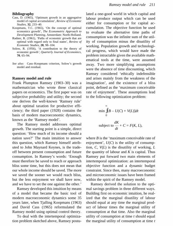
BibliographyCass, D. (1965), ‘Optimum growth in an aggregative

model of capital accumulation’, Review of EconomicStudies, 32, 233–40.

Koopmans, T.C. (1965), ‘On the concept of optimaleconomics growth’, The Econometric Approach toDevelopment Planning, Amsterdam: North-Holland.

Radner, R. (1961), ‘Paths of economic growth that areoptimal with regard only to final states’, Review ofEconomic Studies, 28, 98–104.

Solow, R. (1956), ‘A contribution to the theory ofeconomic growth’, Quarterly Journal of Economics,70, 65–94.

See also: Cass–Koopmans criterion, Solow’s growthmodel and residual.

Ramsey model and ruleFrank Plumpton Ramsey (1903–30) was amathematician who wrote three classicalpapers on economics. The first paper was onsubjective probability and utility; the secondone derives the well-known ‘Ramsey rule’about optimal taxation for productive effi-ciency; the third paper (1928) contains thebasis of modern macroeconomic dynamics,known as the ‘Ramsey model’.

The Ramsey model addresses optimalgrowth. The starting point is a simple, directquestion: ‘How much of its income should anation save?’ The main intuition to answerthis question, which Ramsey himself attrib-uted to John Maynard Keynes, is the trade-off between present consumption and futureconsumption. In Ramsey’s words: ‘Enoughmust therefore be saved to reach or approachbliss some time, but this does not mean thatour whole income should be saved. The morewe saved the sooner we would reach bliss,but the less enjoyment we shall have now,and we have to set the one against the other.’

Ramsey developed this intuition by meansof a model that became the basic tool ofmodern macroeconomic dynamics some 35years later, when Tjalling Koopmans (1963)and David Cass (1965) reformulated theRamsey model using optimal control theory.

To deal with the intertemporal optimiza-tion problem sketched above, Ramsey postu-

lated a one-good world in which capital andlabour produce output which can be usedeither for consumption or for capital ac-cumulation. The objective function he usedto evaluate the alternative time paths ofconsumption was the infinite sum of the util-ity of consumption minus the disutility ofworking. Population growth and technologi-cal progress, which would have made theproblem intractable given the available math-ematical tools at the time, were assumedaway. Two more simplifying assumptionswere the absence of time discounting, whichRamsey considered ‘ethically indefensibleand arises mainly from the weakness of theimagination’, and the existence of a blisspoint, defined as the ‘maximum conceivablerate of enjoyment’. These assumptions leadto the following optimization problem:

∞

min ∫[B – U(C) + V(L)]dt0

dKsubject to — + C = F(K, L),

dt

where B is the ‘maximum conceivable rate ofenjoyment’, U(C) is the utility of consump-tion, C, V(L) is the disutility of working, Lthe quantity of labour and K is capital. ThusRamsey put forward two main elements ofintertemporal optimization: an intertemporalobjective function and a dynamic budgetconstraint. Since then, many macroeconomicand microeconomic issues have been framedwithin the spirit of the Ramsey model.

Ramsey derived the solution to the opti-mal savings problem in three different ways.Building first on economic intuition, he real-ized that the marginal disutility of labourshould equal at any time the marginal prod-uct of labour times the marginal utility ofconsumption at that time. Also the marginalutility of consumption at time t should equalthe marginal utility of consumption at time t

Ramsey model and rule 211

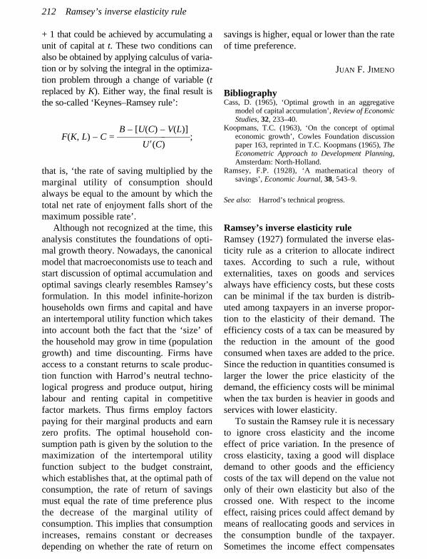
+ 1 that could be achieved by accumulating aunit of capital at t. These two conditions canalso be obtained by applying calculus of varia-tion or by solving the integral in the optimiza-tion problem through a change of variable (treplaced by K). Either way, the final result isthe so-called ‘Keynes–Ramsey rule’:

B – [U(C) – V(L)]F(K, L) – C = ————————;

U�(C)

that is, ‘the rate of saving multiplied by themarginal utility of consumption shouldalways be equal to the amount by which thetotal net rate of enjoyment falls short of themaximum possible rate’.

Although not recognized at the time, thisanalysis constitutes the foundations of opti-mal growth theory. Nowadays, the canonicalmodel that macroeconomists use to teach andstart discussion of optimal accumulation andoptimal savings clearly resembles Ramsey’sformulation. In this model infinite-horizonhouseholds own firms and capital and havean intertemporal utility function which takesinto account both the fact that the ‘size’ ofthe household may grow in time (populationgrowth) and time discounting. Firms haveaccess to a constant returns to scale produc-tion function with Harrod’s neutral techno-logical progress and produce output, hiringlabour and renting capital in competitivefactor markets. Thus firms employ factorspaying for their marginal products and earnzero profits. The optimal household con-sumption path is given by the solution to themaximization of the intertemporal utilityfunction subject to the budget constraint,which establishes that, at the optimal path ofconsumption, the rate of return of savingsmust equal the rate of time preference plusthe decrease of the marginal utility ofconsumption. This implies that consumptionincreases, remains constant or decreasesdepending on whether the rate of return on

savings is higher, equal or lower than the rateof time preference.

JUAN F. JIMENO

BibliographyCass, D. (1965), ‘Optimal growth in an aggregative

model of capital accumulation’, Review of EconomicStudies, 32, 233–40.

Koopmans, T.C. (1963), ‘On the concept of optimaleconomic growth’, Cowles Foundation discussionpaper 163, reprinted in T.C. Koopmans (1965), TheEconometric Approach to Development Planning,Amsterdam: North-Holland.

Ramsey, F.P. (1928), ‘A mathematical theory ofsavings’, Economic Journal, 38, 543–9.

See also: Harrod’s technical progress.

Ramsey’s inverse elasticity ruleRamsey (1927) formulated the inverse elas-ticity rule as a criterion to allocate indirecttaxes. According to such a rule, withoutexternalities, taxes on goods and servicesalways have efficiency costs, but these costscan be minimal if the tax burden is distrib-uted among taxpayers in an inverse propor-tion to the elasticity of their demand. Theefficiency costs of a tax can be measured bythe reduction in the amount of the goodconsumed when taxes are added to the price.Since the reduction in quantities consumed islarger the lower the price elasticity of thedemand, the efficiency costs will be minimalwhen the tax burden is heavier in goods andservices with lower elasticity.

To sustain the Ramsey rule it is necessaryto ignore cross elasticity and the incomeeffect of price variation. In the presence ofcross elasticity, taxing a good will displacedemand to other goods and the efficiencycosts of the tax will depend on the value notonly of their own elasticity but also of thecrossed one. With respect to the incomeeffect, raising prices could affect demand bymeans of reallocating goods and services inthe consumption bundle of the taxpayer.Sometimes the income effect compensates

212 Ramsey’s inverse elasticity rule

the price effect, as happens with certain basicgoods. Taxing these goods would reduce thereal income of the taxpayers and the quantityconsumed of the good would increase.Considering the income effect invalidates theelasticity of demand as an index of consumerreaction to prices and eliminates the signifi-cance of the inverse elasticity rule.

The Ramsey rule was extended andapplied to the optimal regulation of monop-oly prices by Boiteux (1956). The reformula-tion of the idea says that the optimal way toallocate fixed costs among different prod-ucts, in the case of a multi-product monopolyindustry, is to distribute them, moving ahigher proportion of the fixed costs to thoseproducts with lower elasticity of demand.

Assuming that regulators approve pricesas a mark-up over marginal costs, the shareof fixed costs to allocate to each differentproduct (i) will be exactly:

pi – cmi d——— = —‚

pi ei

where p is the price of each product (i), cmthe marginal costs of i, ei the price elasticityof each product demand and d is a constantthat defines the level of prices and is relatedto the Lagrange multiplier of the optimiza-tion process.

The main problems when using theRamsey rule as a regulatory criterion toguide the setting of tariffs or prices are thatobtaining acute and precise informationabout elasticity of the demand of every prod-uct or segment of the market can beextremely difficult for regulators, and thatapplying the inverse elasticity rule couldmean that the burden on the less wealthyconsumers is much higher than the burden onthe wealthier. The distributive consequencesof the rule can make it socially unacceptable.

MIGUEL A. LASHERAS

BibliographyBoiteux, M. (1956), ‘Sur la gestion des monopoles

publics astreints à l’equilibre budgetaire’,Econometrica, 24, 22–40.

Ramsey, F. (1927), ‘A contribution to the theory of taxa-tion’, Economic Journal, 27 (1), 47–61.

Rao–Blackwell’s theoremLet {Pq}q∈ Q be a family of distribution on asample space c, and T be an unbiased esti-mator of d(q) with Eq(T2) < ∞. Let S be asufficient statistic for the family {Pq}q∈ Q.Then the conditional expectation T� = Eq(T/S)is independent of q and is an unbiased esti-mator of d(q). Moreover, Varq(T�) ≤ Varq(T)for every q, and Varq(T�) < Varq(T) for someq unless T is equal to T� with probability 1.

LEANDRO PARDO

BibliographyRohatgi, V.K. (1976), An Introduction to Probability

Theory and Mathematical Statistics, New York:John Wiley and Sons.

Rawls’s justice criterionJohn Rawls (1921–2002) develops a theoryof justice with the aim of generalizing andformalizing the traditional theory of socialcontract proposed by Locke, Rousseau andKant. In his theory, Rawls introduces a char-acterization of the principles of justice, andas a result he presents a criterion of justicebased on considerations of fairness.

Rawls’s justice criterion is founded on thecombination of two principles: the principleof fair equality of opportunity and the differ-ence principle. The difference principle asstated by Rawls implies that social andeconomic inequalities are to be arranged sothat they are to the greatest benefit of theleast advantaged. These principles are to beapplied in a lexicographic order, with a prior-ity of justice over efficiency: fair opportunityis prior to the difference principle, and bothof them are prior to the principle of effi-ciency and to that of maximizing welfare.

According to Rawls’s justice criterion,

Rawl’s justice criterion 213

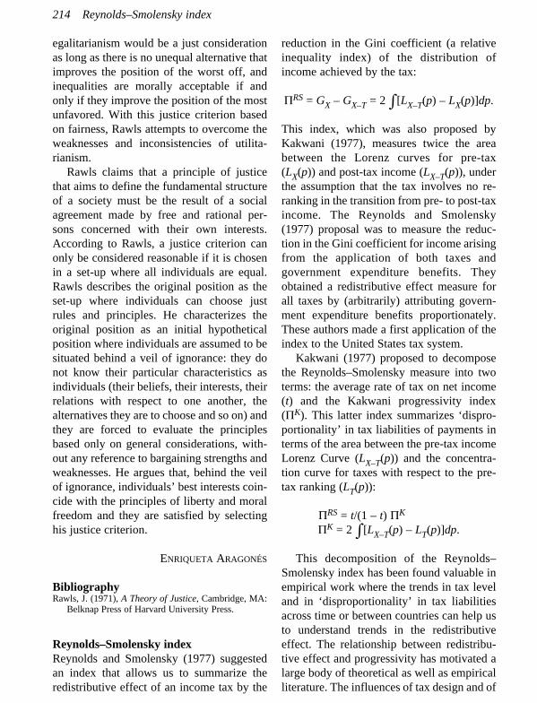
egalitarianism would be a just considerationas long as there is no unequal alternative thatimproves the position of the worst off, andinequalities are morally acceptable if andonly if they improve the position of the mostunfavored. With this justice criterion basedon fairness, Rawls attempts to overcome theweaknesses and inconsistencies of utilita-rianism.

Rawls claims that a principle of justicethat aims to define the fundamental structureof a society must be the result of a socialagreement made by free and rational per-sons concerned with their own interests.According to Rawls, a justice criterion canonly be considered reasonable if it is chosenin a set-up where all individuals are equal.Rawls describes the original position as theset-up where individuals can choose justrules and principles. He characterizes theoriginal position as an initial hypotheticalposition where individuals are assumed to besituated behind a veil of ignorance: they donot know their particular characteristics asindividuals (their beliefs, their interests, theirrelations with respect to one another, thealternatives they are to choose and so on) andthey are forced to evaluate the principlesbased only on general considerations, with-out any reference to bargaining strengths andweaknesses. He argues that, behind the veilof ignorance, individuals’ best interests coin-cide with the principles of liberty and moralfreedom and they are satisfied by selectinghis justice criterion.

ENRIQUETA ARAGONÉS

BibliographyRawls, J. (1971), A Theory of Justice, Cambridge, MA:

Belknap Press of Harvard University Press.

Reynolds–Smolensky indexReynolds and Smolensky (1977) suggestedan index that allows us to summarize theredistributive effect of an income tax by the

reduction in the Gini coefficient (a relativeinequality index) of the distribution ofincome achieved by the tax:

PRS = GX – GX–T = 2 ∫ [LX–T(p) – LX(p)]dp.

This index, which was also proposed byKakwani (1977), measures twice the areabetween the Lorenz curves for pre-tax(LX(p)) and post-tax income (LX–T(p)), underthe assumption that the tax involves no re-ranking in the transition from pre- to post-taxincome. The Reynolds and Smolensky(1977) proposal was to measure the reduc-tion in the Gini coefficient for income arisingfrom the application of both taxes andgovernment expenditure benefits. Theyobtained a redistributive effect measure forall taxes by (arbitrarily) attributing govern-ment expenditure benefits proportionately.These authors made a first application of theindex to the United States tax system.

Kakwani (1977) proposed to decomposethe Reynolds–Smolensky measure into twoterms: the average rate of tax on net income(t) and the Kakwani progressivity index(PK). This latter index summarizes ‘dispro-portionality’ in tax liabilities of payments interms of the area between the pre-tax incomeLorenz Curve (LX–T(p)) and the concentra-tion curve for taxes with respect to the pre-tax ranking (LT(p)):

PRS = t/(1 – t) PK

PK = 2 ∫ [LX–T(p) – LT(p)]dp.

This decomposition of the Reynolds–Smolensky index has been found valuable inempirical work where the trends in tax leveland in ‘disproportionality’ in tax liabilitiesacross time or between countries can help usto understand trends in the redistributiveeffect. The relationship between redistribu-tive effect and progressivity has motivated alarge body of theoretical as well as empiricalliterature. The influences of tax design and of

214 Reynolds–Smolensky index

the pre-tax income distribution upon redis-tributive effect and progressivity has beendetermined and assessed; both indices havebeen decomposed across taxes and extendedto benefits and to evaluating the net fiscalsystem.

However, the former decomposition nolonger holds when re-ranking in the transi-tion from pre- to post-tax income is present.In that case, the decomposition must becorrected by a term capturing the contribu-tion of re-ranking to the redistributive effectof the tax. This term is given by the differ-ence between the Gini coefficient and theconcentration index for post-tax income(Kakwani, 1984).

MERCEDES SASTRE

BibliographyReynolds, M. and E. Smolensky (1977), Public

Expenditure, Taxes and the Distribution of Income:The United States, 1950, 1961, 1970, New York:Academic Press.

Kakwani, N.C. (1977), ‘Measurement of tax progressiv-ity: an international comparison’, Economic Journal,87, 71–80.

Kakwani, N.C. (1984), ’On the measurement of taxprogressivity and redistributive effect of taxes withapplications to horizontal and vertical equity’,Advances in Econometrics, 3, 149–68.

See also: Gini’s coefficient, Kakwani index.

Ricardian equivalenceThis is a proposition according to whichfiscal effects involving changes in the rela-tive amounts of tax and debt finance for agiven amount of public expenditure wouldhave no effect on aggregate demand, interestrates and capital formation. The proposition,as stated above, was not directly introducedby David Ricardo but by Robert Barro, in1974. Although the formal assumptionsunder which this equivalence result holds arequite stringent, the intuition behind it is fairlystraightforward. We need note only twoideas. First, any debt issuance by the govern-ment implies a stream of interest charges and

principal repayments that should be financedin the future by taxation, the current value ofdebt being equal to the present discountedvalue of future required taxation. Second, ifagents behave on the basis of their perceivedpermanent income (wealth), they will alwaysact as if there were no public debt in theeconomy, and the way the governmentfinances their expenditure will have no effecton economic activity.

Interestingly, Barro did not acknowledgein his 1974 paper any intellectual debt toRicardo or to any other classical economist.It was only two years later that JamesBuchanan documented the close connectionbetween Barro’s proposition and somepublic finance analysis contained inRicardo’s Principles of Political Economyand Taxation and, especially, in the essay‘Funding System’, both published two and ahalf centuries earlier than Barro’s paper.Buchanan therefore suggested naming theproposition the ‘Ricardian equivalence the-orem’, a term immediately accepted by Barroand consistently used by the whole profes-sion since.

Some, however, have argued that muchof what Ricardo wrote in 1820 was alreadypresent, albeit with less clarity, in AdamSmith’s Wealth of Nations, published somedecades earlier. Indeed, Smith dwelt on theeconomic effects of both taxation and debtissuance as alternative sources of govern-ment finance, although the equivalenceresult does not emerge in a clear manner.Ricardo’s analysis is much sharper, particu-larly with respect to the first idea expressedabove: in financial terms the governmentcan equally service a debt, issued today foran amount X, if households make a down-payment of X today, to afford to pay taxes inthe future. Much less obvious is whetherRicardo would actually subscribe to thesecond idea behind Barro’s proposition:namely, that the former financial equiva-lence result necessarily implies that public

Ricardian equivalence 215

deficits do not have any meaningfuleconomic effect. Actually, he suggests in‘Funding System’ that people are somewhatmyopic as they would react much more to current than to future expected taxation.At a minimum, it could be contended thatRicardo himself would have been somewhatsceptical about the empirical relevance ofthe ‘Ricardian equivalence theorem’.

In fact, there is no need to resort to agents’irrationality to question the practical applic-ability of Ricardian equivalence. Indeed, asmentioned above, this proposition requires anumber of strong assumptions. In particular,agents must behave as if they were going tolive forever; that is, they must care a lotabout their children (intergenerational altru-ism) or have strong bequest motives.Otherwise, as they would always be able toassign a positive probability of future taxesrequired to service debt being paid by otherpeople after they die, they would feel wealth-ier if government expenditure were financedby debt issuance rather than taxation,thereby making Ricardian equivalence fail.Similarly, the proposition requires thatagents should not be liquidity-constrained, asthey should be able to borrow against futureincome in order for the permanent incomehypothesis to hold. If they were subject toborrowing limits, they would always preferto pay taxes in the future. Actually, theissuance of public debt would help them tomake use now of income that would other-wise only be available for consumption in thefuture. This implies that they would spendmore if government policy favoured debtfinancing over taxation. Finally, Ricardianequivalence relies on the assumption thattaxes are lump-sum. To the extent that taxes were distortionary, the intertemporalsequencing of taxation implied by thegovernment financial strategy would actuallymatter.

It is not difficult to find compellingevidence against each of those important

assumptions required for Ricardian equiva-lence to hold. It is much more difficult,however, to prove that such a failure under-mines the overall empirical plausibility of theproposition. Indeed, the available economet-ric analyses of the issue find it difficult toreject Ricardian hypotheses such as the irrel-evance of public debt or deficits on con-sumption and interest rate equations. Thissuggests that, while it is difficult to refute theidea that the world is not Ricardian, the rela-tionship between government financialpolicy and the real economy does not seem tobe absolutely at odds with the implications ofRicardian equivalence.

FERNANDO RESTOY

BibliographyBarro, R.J. (1974), ‘Are government bonds net wealth?’,

Journal of Political Economy, 82, 1095–118.Ricardo, D. (1820), Funding System, reprinted in P.

Sraffa (ed.) (1951), The Works and Correspondenceof David Ricardo, vol. IV, Cambridge: CambridgeUniversity Press. The original was published as asupplement of the British Encyclopaedia.

Seater, J.J. (1993), ‘Ricardian equivalence’, Journal ofEconomic Literature, 31, 142–90.

Ricardian viceThis is the name given by Schumpeter to themethod used by David Ricardo whereby analready simplified economic model is cutdown by freezing one variable after another,establishing ad hoc assumptions until thedesired result emerges almost as a tautol-ogy, trivially true (Schumpeter, 1954, p.473). The idea that some economists haveused, and abused, this path has led to fruit-ful debates questioning the excessiveabstraction and reductionism in deductiveeconomics.

ESTRELLA TRINCADO

BibliographySchumpeter, Joseph A. (1954), History of Economic

Analysis, New York: Oxford University Press.

216 Ricardian vice

Ricardo effectThis is one of the main microeconomicexplanations for additional savings tendingto be invested in more roundabout and capi-tal-intensive production processes. Increasesin voluntary savings exert a particularlyimportant, immediate effect on the level ofreal wages. The monetary demand forconsumer goods tends to fall wheneversavings rise. Hence it is easy to understandwhy increases in savings ceteris paribus arefollowed by decreases in the relative pricesof final consumer goods. If, as generallyoccurs, the wages or rents of the originalfactor labor are initially held constant innominal terms, a decline in the prices of finalconsumer goods will be followed by a rise inthe real wages of workers employed in allstages of the productive structure. With thesame money income in nominal terms, work-ers will be able to acquire a greater quantityand quality of final consumer goods andservices at consumer goods’ new, morereduced prices. This increase in real wages,which arises from the growth in voluntarysaving, means that, in relative terms, it is inthe interest of entrepreneurs of all stages inthe production process to replace labor withcapital goods. Via an increase in real wages,the rise in voluntary saving sets a trendthroughout the economic system towardlonger and more capital-intensive productivestages. In other words, entrepreneurs nowfind it more attractive to use more capitalgoods than labor. This constitutes a powerfuleffect tending toward the lengthening of thestages in the productive structure.

According to Friedrich A. Hayek, DavidRicardo was the first person to analyzeexplicitly this effect. Ricardo concludes inhis Principles (1817) that

every rise of wages, therefore, or, which is thesame thing, every fall of profits, would lowerthe relative value of those commodities whichwere produced with a capital of a durablenature, and would proportionally elevate those

which were produced with capital more perish-able. A fall of wages would have precisely thecontrary effect.

And in the well-known chapter ‘OnMachinery’, which was added in the thirdedition, published in 1821, Ricardo adds that‘machinery and labour are in constantcompetition, and the former can frequentlynot be employed until labour rises’.

This idea was later recovered by Hayek,who, beginning in 1939, applied it exten-sively in his writings on business cycles.Hayek explains the consequences that anupsurge in voluntary saving has on theproductive structure to detract from theorieson the so-called ‘paradox of thrift’ and thesupposedly negative influence of saving oneffective demand. According to Hayek,

with high real wages and a low rate of profitinvestment will take highly capitalistic forms:entrepreneurs will try to meet the high costs oflabour by introducing very labour-savingmachinery – the kind of machinery which itwill be profitable to use only at a very low rateof profit and interest.

Hence the Ricardo effect is a pure micro-economic explanation for the behavior ofentrepreneurs, who react to an upsurge involuntary saving by boosting their demandfor capital goods and by investing in newstages further from final consumption. It isimportant to remember that all increases involuntary saving and investment initiallybring about a decline in the production ofnew consumer goods and services withrespect to the short-term maximum whichcould be achieved if inputs were not divertedfrom the stages closest to final consumption.This decline performs the function of freeingproductive factors necessary to lengthen the stages of capital goods furthest fromconsumption. In a modern economy, con-sumer goods and services which remainunsold when saving increases fulfill theimportant function of making it possible for

Ricardo effect 217

the different economic agents (workers,owners of natural resources and capitalists)to sustain themselves during the time periodsthat follow. During these periods the recentlyinitiated lengthening of the productive struc-ture causes an inevitable slowdown in thearrival of new consumer goods and servicesat the market. This slowdown lasts until thecompletion of all the new, more capital-intensive processes that have been started. Ifit were not for the consumer goods andservices that remain unsold as a result ofsaving, the temporary drop in the supply ofnew consumer goods would trigger asubstantial rise in the relative price of thesegoods and considerable difficulties in theirprovision.

JESÚS HUERTA DE SOTO

BibliographyHayek, F.A. (1939), ‘Profits, Interest and Investment’

and Other Essays on the Theory of IndustrialFluctuations, reprinted in (1975) London:Routledge, and Clifton: Augustus M. Kelley, p. 39.

Hayek, F.A. (1942), ‘The Ricardo Effect’, Economica, 9(34), 127–52; republished (1948) as chapter 11 ofIndividualism and Economic Order, Chicago:University of Chicago Press, pp. 220–54.

Hayek, F.A. (1969), ‘Three elucidations of the Ricardoeffect’, Journal of Political Economy, 77 (2),March/April; reprinted (1978) as chapter 11 of NewStudies in Philosophy, Politics, Economics and theHistory of Ideas, London: Routledge & Kegan Paul,pp. 165–78.

Ricardo, David (1817), On the Principles of PoliticalEconomy and Taxation, reprinted in Piero Sraffa andM.H. Dobb (eds) (1982), The Works andCorrespondence of David Ricardo, vol. 1,Cambridge: Cambridge University Press, pp. 39–40,395.

Ricardo’s comparative costsIn 1817, David Ricardo (1772–1823) estab-lished the first theoretical and convincingexplanation of the benefits of internationalfree trade and labour specialization, after-wards called the ‘comparative advantageprinciple’. It can be enunciated as follows:even if a country has an absolute cost disad-vantage in all the goods it produces, there

will be one or more goods in which it has acomparative cost advantage with respect toanother country, and it will be beneficial forboth to specialize in the products in whicheach has a comparative advantage, and toimport the rest from the other country. Acountry has absolute advantage in one prod-uct when it produces it at a lower cost thanthe other country. The comparative advan-tage refers to the relative production cost oftwo different goods inside each nation: acountry has comparative advantage in onegood when its production is less costly interms of the other good than it is in the othercountry.

Ricardo used an example of two coun-tries, England and Portugal, producing twogoods, cloth and wine, that has become oneof the most famous in the history ofeconomic thought:

England may be so circumstanced, that toproduce the cloth may require the labour of100 men for one year; and if she attempted tomake the wine, it might require the labour of120 men for the same time. England wouldtherefore find it her interest to import wine,and to purchase it by the exportation of cloth.To produce the wine in Portugal, might requireonly the labour of 80 men for one year, and toproduce the cloth in the same country, mightrequire the labour of 90 men for the same time.It would therefore be advantageous for her toexport wine in exchange for cloth. Thisexchange might even take place, notwithstand-ing that the commodity imported by Portugalcould be produced there with less labour thanin England. Though she could make the clothwith the labour of 90 men, she would import itfrom a country where it required the labour of100 men to produce it, because it would beadvantageous to her rather to employ her capi-tal in the production of wine, for which shewould obtain more cloth from England, thanshe could produce by diverting a portion of hercapital from the cultivation of vines to themanufacture of cloth. (Ricardo, 1817, ch. 7)

This text contains the essence of the principleof comparative advantage. Even though

218 Ricardo’s comparative costs

Ricardo did not quantify the gains obtainedby both countries after the specialization, asimple exercise will show that he was right.Suppose that, in England, the cost of produc-ing a piece of cloth is 10 hours of labour, and12 for a litre of wine. In Portugal these costsare, respectively, nine and eight hours.Portugal has absolute cost advantage in theproduction both of wine and of clothes. Butin England wine is comparatively morecostly than cloth, as it requires two morehours; and in Portugal the less expensiveproduct is wine. This means that England hasa comparative cost advantage in the produc-tion of cloth, while Portugal has it in theproduction of wine, as follows.

If we measure the market value of prod-ucts in terms of hours of work, as Ricardodoes, we can deduce, for instance, that inEngland with one piece of cloth (value = 10hours) it is possible to buy less than a litre ofwine (10/12 litres), as a litre of wine requiresin England 12 hours of labour to beproduced. But in Portugal with the samepiece of cloth it is possible to buy more thana litre of wine (9/8 litres). So to exchange apiece of cloth for wine it is better to go toPortugal – if we assume, as Ricardo does,free trade between both countries. It seemsclear, then, that England benefits fromspecializing in the production of cloth andimporting wine from Portugal. The samereasoning leads to the conclusion that, forPortugal, the best option is to specialize inthe production of wine, in which she hascomparative advantage, and import clothfrom England.

Ricardo proved that specialization andtrade can increase the living standards ofcountries, independently of their absolutecosts. His theory was presented during thedebates about the growing level of cornprices in England, and Ricardo, as manyothers, argued that protectionism was one ofits main causes. His argument served as afirm basis for the promoters of free trade, and

was decisive in abolishing the protectionistCorn Laws in 1846.

JOSÉ M. ORTIZ-VILLAJOS

BibliographyBlaug, Mark (ed.) (1991), David Ricardo (1772–1823),

Pioneers in Economics 14, Aldershot, UK andBrookfield, US: Edward Elgar.

De Vivo, G. (1987), ‘Ricardo, David (1772–1823)’, in J.Eatwell, M. Milgate and P. Newman (eds), The NewPalgrave. A Dictionary of Economics, vol. 4,London: Macmillan, pp. 183–98.

Ricardo, David (1817), On the Principles of PoliticalEconomy and Taxation, reprinted in P. Sraffa (ed.)(1951), The Works and Correspondence of DavidRicardo, vol. I, Cambridge: Cambridge UniversityPress.

Ricardo–Viner modelJacob Viner (1892–1970) extended theRicardian model by including factors otherthan labor, and by allowing the marginal prod-uct of labor to fall with output. TheRicardo–Viner model was later developed andformalized by Ronald Jones (1971). MichaelMussa (1974) provided a simple graphicalapproach to illustrate the main results. Itconstitutes a model in its own right, but it canalso be viewed as a short-term variant of theHeckscher–Ohlin model, with capital immo-bile across sectors. Capital and land inputs arefixed but labor is assumed to be a variableinput, freely and costlessly mobile betweentwo sectors. Each of the other factors isassumed to be specific to a particular industry.Each sector’s production displays diminishingreturns to labor. The model is used to explainthe effects of economic changes on labor allo-cation, output levels and factor returns, and isparticularly useful in exploring the changes inthe distribution of income that will arise as acountry moves from autarky to free trade.

YANNA G. FRANCO

BibliographyJones, Ronald W. (1971), ‘A three-factor model in

theory, trade and history’, in J.N. Bhagwati, R.A.

Ricardo–Viner model 219

Mundell, R.W. Jones and J. Vanek (eds), Trade,Balance of Payments, and Growth: Essays in Honorof C.P. Kindleberger, Amsterdam: North-Holland,pp. 3–21.

Mussa, Michael (1974), ‘Tariffs and the distribution ofincome: the importance of factor specificity, substi-tutability and intensity in the short and long run’,Journal of Political Economy, 82 (6), 1191–203.

See also: Heckscher–Ohlin theorem, Ricardo’s com-parative costs.

Robinson–Metzler conditionNamed after Joan Robinson and Lloyd A.Metzler, although C.F. Bickerdike, J.E.Meade and others contributed to the idea andare sometimes linked to the eponym, thecondition refers to a post-devaluation tradebalance adjustment under a comparativestatic approach in the context of internationalequilibrium and under a system of fluctuat-ing exchange rates. The adjustment analysisis applied through elasticity both in exportsand in imports. The Robinson–Metzlercondition focuses on the four elasticities inplay, in order to predict the global result ofall the adjustments that determine the newbalance of trade: the foreign elasticity of demand for exports, the home elasticity ofsupply for exports, the foreign elasticity of supply for imports, and the home elastic-ity of demand for imports. The final balance oftrade will depend on the intersection of all ofthem.

ELENA GALLEGO

BibliographyBickerdike, Charles F. (1920), ‘The instability of

foreign exchange’, Economic Journal, 30, 118–22.Robinson, Joan (1950), ‘The foreign exchanges’, in

Lloyd A. Metzler and Howard S. Ellis (eds),Readings in the Theory of International Trade,London: George Allen and Unwin, pp. 83–103.

See also: Marshall–Lerner condition.

Rostow’s modelWalt Whitman Rostow’s (1916–2003) modelis a stages theory of economic development.

Rostow divided ‘the process of economicgrowth’ (that was the title of one of hisbooks) into five ‘stages of economic growth’(the title of his most famous book). Thesestages are traditional society, the setting ofthe preconditions for growth, the ‘take-off’into self-sustained growth, the drive towardseconomic maturity, and the age of high massconsumption.

Little explanation is required about themeaning and nature of these stages.Traditional society is characterized by‘limited production functions based on pre-Newtonian science’. This early stage is not unlike Joseph Schumpeter’s ‘circularflow’, which occupies a similar place inSchumpeter’s theory of economic develop-ment. The preconditions for growth entail aseries of social changes which are previousto industrialization: improvement of politicalorganization (‘the building of an effectivecentralized national state’), new social atti-tudes, a drop in the birth rate, an increase inthe investment rate, a jump in agriculturalproductivity. The third stage, the take-off, iscentral to the model in more than one way. Itbrings about the most radical and swift socialchange: an approximate doubling in the rateof investment and saving, fast political andinstitutional modernization, and rapid indus-trialization. Two distinctive features ofRostow’s take-off are that it is spearheadedby a limited number of ‘leading sectors’,whose rate of growth is higher than those ofother, following sectors, which in turn aredivided into ‘supplementary growth’ and‘derived growth’ sectors; and that it is rela-tively brief, spanning a generation.

The other two stages are less interestingfrom a theoretical point of view. There is,however, a key phrase in The Stages ofEconomic Growth (p. 58) which summarizesthe basic idea behind the model: ‘By andlarge, the maintenance of momentum for ageneration persuades the society to persist, toconcentrate its efforts on extending the tricks

220 Robinson–Metzler condition

of modern technology beyond the sectorsmodernized during the take-off.’ It is thispersistence which leads the modernizedeconomy into the drive to maturity, which ischaracterized as ‘the period when a societyhas effectively applied the range of [. . .]modern technology to the bulk of itsresources’. Once society has successfullyperformed its take-off, its own self-propelledinertia drives it into maturity and massconsumption or ‘post-maturity’, when, prob-lems of supply being solved, attention shiftsto ‘problems of consumption, and of welfarein the widest sense’.

This model, which had a tremendous echoin the 1960s and 1970s among academics,politicians and even a wide lay audience,elicits a few comments. First of all, Rostow’smodel belongs to a wide group of stagestheories of historical development, especiallythose relating to economic history, fromRoscher and Hildebrand to Colin Clark andGerschenkron, through Marx and Schmoller.Second, it combines a stylized descriptionand periodization of western economichistory with some economic theories much invogue in the 1950s and 1960s, such as theHarrod–Domar conditions for balancedgrowth. Rostow was a student of the BritishIndustrial Revolution and his model is a goodfit with British modern economic history. Healso allowed for a variant of the model, thatof the ‘born-free’ countries, those ex-colonies without a medieval past, such as theUnited States and Canada, which were bornto nationhood already in the preconditionsstage.

Third, its key idea and most originalfeature is expressed by his statements about‘persistence’ and ‘self-sustained growth’:according to Rostow’s model, when an econ-omy has crossed a certain threshold of devel-opment, there is an inertia that keeps itgrowing. Hence its attractive aeronauticalmetaphor: once an airplane has overcomegravity in take-off, it (normally) stays

airborne. Fourth, Rostow’s model had clearand intended political implications, whichwere expressed in the subtitle of The Stages:A Non-Communist Manifesto. He explicitlytried to offer an alternative interpretation ofmodern history to Karl Marx’s vision. In sodoing, Rostow drew an optimistic picture ofthe Soviet Union’s economic development,viewing it as parallel to the growth of theUnited States and gave support to the theoryof convergence of capitalism and commu-nism, much in vogue at the time.

Naturally, Rostow’s model provokedheated debate, all the more so since its authorwas a close adviser to Presidents Kennedyand Johnson, and an ardent supporter of theVietnam War. Henry Rosovsky spoke about‘the take-off into self-sustained controversy’;Phyllis Deane, for instance, denied thatBritish investment rates were as high duringtake-off as Rostow stated, and Robert Fogelstudied the development of American rail-ways to deny that they played the role of lead-ing sector that Rostow attributed to them.Gerschenkron pointed out that there is nodefinite set of preconditions or ‘prerequi-sites’, and that the different growth pathsfollowed by diverse countries were largelyresults of varying arrays of developmentassets. It has also been remarked that,contrary to Rostow’s specific predictions,some countries, such as Argentina, Russia orChina, had very long take-offs, which in factwere partial failures, something the model didnot account for. Many other criticisms couldbe cited, but Rostow’s model and terminol-ogy have endured, if not for their explanatorypower, at least for their descriptive value.

GABRIEL TORTELLA

BibliographyGerschenkron, Alexander (1962): ‘Reflections on the

concept of “prerequisites” of modern industrializ-ation’, Economic Backwardness in HistoricalPerspective, Cambridge, MA: Harvard UniversityPress, pp. 31–51.

Rostow’s model 221

Rostow, W.W. (1953), The Process of EconomicGrowth, Oxford: Clarendon Press.

Rostow, W.W. (1960), The Stages of Economic Growth.A Non-Communist Manifesto, Cambridge: Cam-bridge University Press.

See also: Gerschenkron’s growth hypothesis, Harrod–Domar model.

Roy’s identityRoy’s identity is a consequence of the dual-ity of utility maximization and expenditureminimization in consumer theory, and relatesthe Walrasian demand to the price derivativeof the indirect utility function. It can beproved as a straightforward application of theenvelope theorem. The importance of Roy’sidentity is that it establishes that the indirectutility function can legitimately serve as abasis for the theory of demand. Formally,Roy’s identity states the following.

Suppose that u(x) is a continuous utilityfunction representing a locally non-satiatedand strictly convex preference relationdefined on the consumption set RL

+, wherex∈ RL

+. Suppose that the indirect utility func-tion v(p, m) is differentiable at (p, m ) >> 0,where p = (p1, p2, . . ., pL) is a given vector ofprices of goods 1, 2, . . ., L, and m is a givenlevel of income. Let x(p, m) be the Walrasiandemand function. Then, for every l = 1, 2, . . ., L, the Walrasian demand for good 1,xl(p, m), is given by

∂v(p, m)/∂plxl(p, m) = – —————.

∂v(p, m)/∂m

As an example, let L = 2 and let the utilityfunction be Cobb–Douglas, given by u(x) =x1x2. Maximizing the utility function subjectto the budget constraint p1x1 + p2x2 = m yieldsthe two Walrasian demand functions x1( p, m)= m/2pl, l = 1, 2. The indirect utility functionis obtained by substituting the demand func-tions back into the utility function, v( p, m) =m2/4p1p2. Applying Roy’s identity, werecover the Walrasian demand functions

∂v( p, m)/∂pl m– ————— = —— = xl( p, m), for l = 1, 2.

∂v( p, m)/∂m 2pl

CRISTINA MAZÓN

BibliographyRoy, René (1942), De l’utilité, Contribution à la théorie

des choix, Paris: Hermann & Cie

Rubinstein’s modelTwo players bargain over the partition of asurplus of fixed size normalized to one.They take turns to make offers to each otheruntil agreement is secured. Player 1 makesthe first offer. If the players perpetuallydisagree then each player’s pay-off is zero.They are assumed to be impatient with thepassage of time and share a commondiscount factor of d ∈ (0, 1) so that a euroreceived in period t is worth dt–1, where t ∈{1, 2, 3 . . .}. This infinite-horizon bargain-ing game with perfect information, due toRubinstein (1982), has many Nash equilib-ria: any partition of the surplus can beobtained in an equilibrium. Nevertheless,this game has a unique subgame-perfectequilibrium. In this equilibrium, the playersreach an inmediate agreement in period 1,with player 1 earning 1/(1 + d) and player 2earning d/(1 + d). Let M and m denoterespectively the supremum and the infimumof the continuation pay-offs of a player inany subgame-perfect equilibrium of anysubgame that begins in period t with thisplayer making an offer. As the responderwill be the proposer in period t + 1 his reser-vation values in t are dM and dm. Therefore,by subgame perfection, the followinginequalities should hold: M ≤ 1 – dm , and m≥ 1 – dM. It follows that M = m = 1/(1 + d).So a player’s subgame-perfect equilibriumpay-off is uniquely determined.

The subgame-perfect equilibrium strat-egies are as follows: a player who receivesan offer accepts it if and only if he is offered

222 Roy’s identity

at least d/(1 + d), while, when he has tomake a proposal, offers exactly d/(1 + d) tothe other player. To see that the equilibriumstrategies are unique, notice that, after everyhistory, the proposer’s offer must beaccepted in equilibrium. If players havedifferent discount factors d1 and d2, a simi-lar reasoning, using the stationarity of thegame, proves that the equilibrium partitionis (v, 1 – v) where v = (1 – d2)/(1 – d1d2).This is one of the main insights ofRubinstein’s model. A player’s bargainingpower depends on the relative magnitude ofthe players’ respective costs of makingoffers and counter-offers, with the absolutemagnitudes of these costs being irrelevantto the bargaining outcome.

Define di = exp(–riD), i = 1, 2, where D >0 is the time interval between consecutiveoffers and ri > 0 is player i’s discount factor.It is straightforward to verify that the limit-ing, as D → 0, subgame-perfect equilibriumpay-offs pair (v, 1 – v) is identical to theasymmetric Nash bargaining solution of thisbargaining problem.

This basic alternating offers game is astylized representation of two features thatlie at the heart of most real-life negotiations.On the one hand, players attempt to reach anagreement by making offers and counter-offers. On the other hand, bargainingimposes costs on both players. Such a gameis useful because it provides a basic frame-work upon which richer models of bargain-ing and applications can be built.

GONZALO OLCINA

BibliographyRubinstein, A. (1982), ‘Perfect equilibrium in a bargain-

ing model’, Econometrica, 50, 97–109.Shaked, A. and J. Sutton (1984), ‘Involuntary unem-

ployment as a perfect equilibrium in a bargainingmodel’, Econometrica, 52, 1351–64.

See also: Nash bargaining solution, Nash equilibrium.

Rybczynski theoremOne of the building blocks of theHeckscher–Ohlin model, the Rybczynskitheorem, named after the Polish economistTadeusz Mieczyslaw Rybczynski (b.1923),is the symmetric counterpart to the Stolper–Samuelson theorem. Just as the latterdemonstrates the close link connectingcommodity prices to factor prices, theformer proves, under suitable conditions, theexistence of a well-defined relationshipbetween changes in factor endowments andchanges in the production of goods in theeconomy.

The following assumptions, standard inthe Heckscher–Ohlin model, are set: theeconomy is made up of two sectors, eachproducing a homogeneous good (X and Y) byemploying two factors, named labor (L) andcapital (K), under constant returns to scale;the total endowment of each factor is fixed tothe economy and both factors are perfectlymobile across sectors; there are no transac-tion costs or taxes and competition prevailsthroughout. It is further assumed that oneindustry (say X) is more capital-intensivethan the other (Y). Then the theorem statesthat, if relative prices are held constant, anincrease in the quantity of one factor ‘mustlead to an absolute expansion in productionof the commodity using relatively much ofthat factor and to an absolute curtailment ofproduction of the commodity using relativelylittle of the same factor’ (Rybczynski, 1955,(p. 338).

This result, easily proved using theEdgeworth box or elementary algebra,agrees with economic intuition. First, noticethat, for good prices to be constant, factorprices have to be constant too, and thisentails, given constant returns to scale, thatfactor intensities have to remain unchangedin both industries as well. Let us nowsupose an increase in the total endowmentof one factor, say labor. To keep factorintensities constant, the extra labour has to

Rybczynski theorem 223

be allocated to the labor-intensive industry(Y) where it will be combined with capitalreleased from X (made available by thecontraction of production in X). But X,being capital-intensive, releases more capi-tal per unit of labor as its production goesdown. Hence production goes up in Y bymore than the increase in the labor endow-ment, the excess production being afforded

by the contraction of the production of thecapital-intensive sector.

TERESA HERRERO

BibliographyRybczynski, T.M. (1955), ‘Factor endowments and rela-

tive commodity prices’, Economica, 22, 336–41.

See also: Heckscher–Ohlin theorem, Jones’s magnifi-cation effect, Stolper–Samuelson theorem.

224 Rybczynski theorem

Samuelson conditionPaul A. Samuelson (b.1915, Nobel Prize1970) is one of the most influential economists of the twentieth century.Trained in Harvard University by Hansen,Schumpeter and Leontief, he developedmost of his prolific work in the MIT. Hiswide range of studies covers nearly allbranches of economic theory. An outstand-ing contribution to macroeconomics is theoverlapping generations model of generalequilibrium (1958). Its application topublic finance results in the conditionpresented here which refers to the sustain-ability of a pay-as-you-go pension system.According to Samuelson, a pension systemwill remain balanced if and only if its average internal rate of return does notexceed the growth rate of the fiscal base,which, under the assumption of a constanttax rate, is equal to the growth rate ofemployment plus the growth rate of theaverage wage.

The simplest version of the model, whereindividuals live only two periods (during thefirst one they work and pay contributions andin the second they receive a pension) allowsus to obtain easily the Samuelson condition.If Nt represents the population born in periodt, n is the growth rate of population and r itssurvival rate, the financial surplus of a pay-as-you-go pension system, Bt, can beexpressed as

Bt = t(wtetNt) – ar(wt–1et–1Nt–1), (1)

where t is the contribution rate, wt the realwage, et the employment rate and a thepercentage of the fiscal base received as apension. As stated by equation (1), thesystem has a surplus in period t if

et ar—— (1 + n) (1 + g) ≥ ——, (2)et–1 t

where g is the growth rate of wages. The leftside of (2) is the growth rate of the system’sincome, which, when the employment rate, e,remains constant, is almost equal to 1 + n + g.The right side of (2) is equal to 1 + r, where ris the internal rate of return of the pensionsystem, since individuals pay twt–1 andreceive awt–1 with probability r. Then, substi-tuting in (2) we get the classical Samuelsonproposition of financial equilibrium in a pay-as-you-go pension system: n + g ≥ r.

JORDI FLORES PARRA

BibliographySamuelson, P.A. (1958), ‘An exact consumption–loan

model of interest with or without the socialcontrivance of money’, Journal of PoliticalEconomy, 66 (6), 467–82.

Sard’s theoremThe American mathematician Arthur Sard(1909–80), Professor at Queens College,New York, made important contributions infields of mathematics such as linear approxi-mation and differential topology. Sard’stheorem is a deep result in differential topol-ogy that is a key mathematical tool to showthe generic local uniqueness of the Walrasianequilibria.

Let U be an open set of Rn and let F be acontinuously differentiable function from Uto Rm. A point x∈ U is a critical point of F ifthe Jacobian matrix of F at x has a ranksmaller than m. A point y∈ Rm is a criticalvalue of F if there is a critical point x∈ U withy = F(x). A point of Rm is a regular value ofF if it is not a critical value.

225

S

Sard’s theorem states as follows. Let p >max (0, n – m). If F is a function of class Cp

(that is, all the partial derivatives of F to thepth order included, exist and are continuous),then the set of critical values of F hasLebesgue measure zero in Rm.

A model of exchange economy with aunique equilibrium requires very strongassumptions and, thus, economies withmultiple equilibria must be allowed for. Sucheconomies provide a satisfactory explanationof equilibrium and allow the study of stab-ility provided that all the equilibria of theeconomy are locally unique. In the commonsituation in which the set of equilibria iscompact, local uniqueness is equivalent tofiniteness.

In Debreu (1970) an exchange economywith n consumers is defined by an n-tuple ofdemand functions and an n-tuple of initialendowments e = (e1, . . ., en). If the demandsremain fixed an economy is actually definedby the initial endowments e. Let W(e) denotethe set of all equilibrium prices of the econ-omy defined by e. Under middle assumptionsand using Sard’s theorem, it is shown that theset of initial endowments for which theclosure of W(e) is infinite has zero measure.

On the other hand, in Smale (1981),Sard’s theorem and market-clearing equa-tions have been used, rather than fixed pointmethods, to show equilibrium existence and,in a constructive way, to find the equilibriumpoints.

CARLOS HERVÉS-BELOSO

BibliographyDebreu, G. (1970), ‘Economies with a finite set of equi-

libria’, Econometrica, 38 (3), 387–92.Sard, A. (1942), ‘The measure of the critical points of

differentiable maps’, Bull. Amer. Math. Soc., 48,883–90.

Smale, S. (1981), ‘Global analysis and economics’, in K.Arrow and M. Intriligator (eds), Handbook ofMathematical Economics, Amsterdam: North-Holland, ch. 8.

Sargan testSargan tests, named after John Denis Sargan(b.1924), are specification tests for a class oflinear and non-linear econometric models.The hypothesis under test is the set of over-identifying restrictions arising from theorthogonality conditions required for instru-mental variable (IV) estimation. The teststatistics have become a standard comple-ment when reporting IV estimates. InSargan’s own words (1958), they provide ‘asignificance test for the hypothesis that thereis a relationship between the suggested vari-ables with a residual independent of all theinstrumental variables’. In order to illustratethe form of the test statistic, consider themodel yt = x�tb0 + ut where xt and b0 are q ×1 vectors of predetermined variables andparameters, respectively. Let zt denote an r ×1 vector of predetermined instrumental vari-ables, so E(ztut) = 0 with r > q. (If x’s and z’scontain (independent) measurement errors,the disturbance ut includes both the struc-tural shock and a linear combination ofmeasurement errors). In standard matrixnotation, consider the residuals u = y – Xbwhere

b = [X�Z(Z�Z)–1Z�X]–1 X�Z(Z�Z)–1Z�y

is the optimally weighted IV estimator.Sargan’s test statistic is

u�Z(Z�Z)–1Z�uJ = T ——————.

u�u

Under the null and under suitable regu-larity conditions, its limiting distribution ischi-square with r – q degrees of freedom. Alarge value will lead to rejection. If theorthogonality conditions are satisfied thevector

1— Z�uT

226 Sargan test

of sample covariances should be small,allowing for sampling variation. The teststatistic is a quadratic form of

1— Z�uT

where the weighting matrix corrects forsampling variation and the use of residuals toreplace unobservable disturbances.

Sargan (1958) proposed the test andderived its asymptotic distribution under thenull in the framework of a linear modelwhich explicitly allowed for both simulta-neity and measurement errors. His originalmotivation was the estimation of macroeco-nomic models using time series data. InSargan (1959) he considered a generalizationto nonlinear-in-parameters IV models.Hansen (1982) extended this type of specifi-cation test to a more general non-lineargeneralized method of moments (GMM)framework with dependent observations; thisis the well known ‘J-test’ of overidentifyingrestrictions. For a discussion of the connec-tion between Sargan’s work and the GMM,see Arellano (2002).

PEDRO MIRA

BibliographyArellano, M. (2002), ‘Sargan’s instrumental variable

estimation and GMM’, Journal of Business andEconomic Statistics, 20, 450–59.

Hansen, L.P. (1982) ‘Large sample properties of gener-alized method of moments estimation’, Econo-metrica, 50, 1029–54.

Sargan, J.D. (1958), ‘The estimation of economic rela-tionships using instrumental variables’, Econo-metrica, 26, 393–415.

Sargan, J.D. (1959), ‘The estimation of relationshipswith autocorrelated residuals by the use of instru-mental variables’, Journal of the Royal StatisticalSociety, Series B, 21, 91–105.

Sargant effectThis refers to an increase in the supply ofsavings in the economy caused by a fall inthe rate of interest. Philip Sargant Florence

(1890–1982) pointed out that a continuousdecrease in the interest rate in a period ofrecession could be accompanied by anincrease in annual additions to the capitalstock, as individuals who save in order toobtain a periodical revenue from their capitalwill have to save more. Alfred Marshallconsidered the Sargant effect as an exceptionto the theory that states that the short-runsavings supply curve is positively sloped. Hesaid that, as a consequence of human nature,a decrease in the interest rate will generallytend to limit wealth accumulation, becauseevery fall in that rate will probably drivepeople to save less than they otherwisewould have done (Marshall, 1890, p. 195).Gustav Cassel criticized Sargant’s theory byassuming that, as people can save only acertain amount of their present income, a fallin the rate of interest does not increase thesupply of savings, but it lengthens the periodduring which they will have to save (Blaug,1996, pp. 386, 501).

JAVIER SAN JULIÁN

BibliographyBlaug, Mark (1996), Economic Theory in Retrospect,

5th edn, Cambridge: Cambridge University Press.Marshall, Alfred (1890), Principles of Economics, 8th

edn 1920; reprinted 1977, London: Macmillan.

Say’s lawJean-Baptiste Say (1767–1832) was born inLyons to a protestant family of textile manu-facturers. After a political career marked byhis opposition to Napoleonic autocracy, hecame to manage a textile firm himself. Hisintellectual efforts were directed at establish-ing the foundations of a spontaneouslyordered free society, after the disorders of theFrench Revolution had led public opinion tobelieve that harmony and progress demandeddirection from the centre. After the fall ofNapoleon, he taught the first public course ofpolitical economy in France and in 1830 tookover the chair in Political Economy of the

Say’s law 227

Collège de France. He debated with the clas-sical economists in England, and spread theteachings of Adam Smith on the continent ofEurope.

According to Say’s law, ‘products alwaysexchange for products’. This as yet incom-plete formulation is to be found in the Traitéd’économie politique (1st edn, 1803). Themore complete version, called ‘la loi desdébouchés’ according to which ‘productiongenerates its own demand’ and thereforeevery output will in the end find an outlet, wasformulated by Say after reading James Mill.For Say, as for the majority of classical econ-omists, exchanges in the market are to be seenas barter trades: a general glut was impossiblesince taking a good to market implies effec-tively demanding another good in exchange.

The first critics of this theory, such asLauderdale, Malthus or Sismondi, pointedout that cyclical crises are an observable fact.They variously underlined the danger that thepresent level of output could not be sustainedunless people were ready to exert themselvessufficiently to acquire power to consume, orunless the ‘value’ of the output was main-tained by high prices. Malthus in particularproposed an artificial boost to unproductiveconsumption and increases in the level ofagricultural protection to create a vent forsurplus output. Later in the century, Marxadded that crises would increase in frequencyand harshness, leading to the collapse of thecapitalist system.

The elements of Say’s law are as follows:

1. Money only facilitates barter andchanges nothing in the real world.

2. Savings are always invested and spent.This idea is also to be found in Turgotand Smith.

3. Saving rather than consumption is thesource of economic growth.

James Mill independently discovered thisprinciple when criticising Lauderdale’s excess

investment theory in 1804 and then devel-oped it in Commerce Defended (1808), wherehe did not forget to mention Say. Hisimprovement of the principle that outputgenerates its own demand adds the following:

4. The necessary and spontaneous equalityof production and demand in the econ-omy as a whole springs from the fact thattotal output is necessarily equivalent tototal purchasing power since the rewardsof labour, capital and land reaped inproduction become the demand forgoods and services.

5. Though total demand and supply mustbe equivalent, disproportionalities canarise within the economy because ofindividual miscalculations. These dispro-portionalities explain crises, which mustbe partial and temporary in a properlyfunctioning economy.

Thus, for the earlier classical economists,an insufficiency of aggregate demand isimpossible; indeed there is no such thing as‘aggregate demand’. What appears to be ageneral crisis is really a temporary lack ofharmony in the supply and demand of someparticular goods and services. Even in thedeepest of crises there is demand for manygoods and the redundant stock of output canbe placed when prices fall sufficiently. Thisis also applicable to unemployment.

John Stuart Mill, in his essay, ‘Of theInfluence of Consumption upon Production’(MS 1829–30, 1844), introduced money andcredit into the model:

6. Crises are always partial and arepreceded by investment mistakes owingto which there is excess supply of theoutput of such investment, for whoseproducts people do not want to pay aprice covering costs.

7. As money is not only a means ofpayment but also a store of value, in a

228 Say’s law

monetary economy it is possible to sellwithout buying. Such hoarding increaseswhen confidence starts to fail because ofinvestment errors becoming apparent. Ina credit economy, the effect of hoardingis magnified by a flight to liquidity andbankruptcy spreads through the economy.

8. All this takes on the appearance of ageneral slump that will, however, quicklyand spontaneously correct if prices,wages and interest rates adjust.

Léon Walras, in his Éléments d’économiepolitique pure (1874), gave a more completeformulation of Say’s law, known today asWalras’s law: as a consequence of basicinterrelations among individuals in a generalequilibrium system, the sum of the value ofexcess demands must be zero.

A new wave of criticism rose againstSay’s law with Keynes (1936): an excessivepropensity to save could lead to aggregateconsumption being too weak for aggregateproduction to take off. The result could beattempted overinvestment, a fall in nationalincome and an increase in involuntary unem-ployment.

Once facts refuted early Keynesianism,economists returned to Say’s law under theguise of rational expectations theory: allavailable information is discounted intocurrent decisions by speculators and there-fore markets clear. Hence, as Turgot–Smith,Say, and J. and J.S. Mill say, there can be nogeneral gluts and whatever cyclical phenom-ena may recur will be due to real dispropor-tions caused by technological shocksdisplacing inferior investments. Those co-movements will correct, the more flexibledemand and supply prices are.

PEDRO SCHWARTZ

BibliographyKeynes, J.M. (1936), The General Theory of

Employment Interest and Money, London: Mac-millan.

Mill, James (1808), Commerce Defended, London: C.and R. Baldwin.

Mill, John Stuart (MS 1829–30, 1844), ‘Of the influenceof consumption upon production’, Essays on SomeUnsettled Questions of Political Economy, reprinted1967, Collected Works, vol. IV, University ofToronto Press.

Say, Jean Baptiste (1803), Traité d’économie politique,2nd edn, 1814; reprinted 1971, ‘Des Débouchés’,Livre Premier, Chapitre XV, Paris: Calmann-Lévy,137–47.

Sowell, Thomas (1972), Say’s Law. An HistoricalAnalysis, Princeton: Princeton University Press.

See also: Turgot–Smith theorem, Walras’s law.

Schmeidler’s lemmaConsider an economy with a continuum ofagents where endowments and preferences ofall agents are common knowledge. Assumealso that agents can form groups (coalitions)binding themselves to any mutually advanta-geous agreement. In this economy we definethe core as the set of allocations that cannotbe improved upon by any coalition. Theconcept of the core allows an extension ofthe first welfare theorem stating that aWalrasian equilibrium cannot be blocked bythe coalition of the whole. This is an import-ant result that relies on a very demandinginformational assumption. It is often the casethat agents have knowledge of the character-istics of a limited number of other agents.Alternatively, we can think of transactioncosts of forming coalitions, or of institutionalconstraints putting an upper limit on the sizeof coalitions. Under any of these interpreta-tions, the lack of communication between theagents restricts the set of coalitions that canbe formed. Schmeidler’s lemma says that,given an economy with S agents and a coali-tion E blocking an allocation by means of anallocation f, we can find an arbitrarilysmaller sub-coalition of positive measure,v(F) <= e that also blocks the same allocationusing f.

Formally, let (S, ∑, l) be an atomlessmeasure space, f, g: S → Rn be l-integrablefunctions, and v be a finite measure on ∑,

Schmeidler’s lemma 229

absolutely continuous with respect to l.Given a set E ∈ ∑ such that l(E) > 0 and∫E fdl = ∫Egdl, then for every positive numbere there is a ∑-measurable subset of E, say F,such that: l(F) > 0, v(F) <= e and ∫F fdl =∫Fgdl.

Mas-Colell provides an interesting inter-pretation of this result by considering that theeconomy only needs a few well-informedagents to reach a Walrasian equilibrium.These few agents would be the arbitrageurs.That is, with most of the agents in the econ-omy being passive, it would be enough for asmall profit-maximizing group of agentsperforming optimally to place the economyin equilibrium.

XAVIER MARTINEZ-GIRALT

BibliographySchmeidler, D. (1972), ‘A remark on the core of an

atomless economy’, Econometrica, 40 (3), 579–80.

Schumpeter’s visionIn his 1954 History of Economic Analysis,J.A. Schumpeter (1883–1950) stated that‘analytic effort is of necessity preceded by apreanalytic cognitive act that supplies theraw material for the analytic effort. In thisbook, this preanalytic cognitive act will becalled Vision’ (p. 41). We ‘see things in alight of’ our vision (Schumpeter’s emphasis).This is sometimes called ‘ideology’, ‘worldview’, ‘cosmovision’ or, after Kuhn (1962),‘paradigm’.

Schumpeter is talking about ‘the dangersof ideological bias’ and how to detect andeliminate ideological elements through standard scientific procedure. Despite anyoriginal inevitable contamination, the scien-tific process, through ‘factual work and theoretical work’ (called poetically bySchumpeter ‘the cold steel of analysis’)refines and completes the original vision and will ‘eventually produce scientificmodels’, that is, value-free positive econom-

ics. So Schumpeter’s position is similar toFriedman’s (1953): ideology is one of thepossible legitimate motivations of a research,but not relevant for the correctness of itsresult; ‘explanation, however correct, of thereasons why a man says what he says tells usnothing about whether it is true or false’(Schumpeter, 1954, p. 36).

But throughout the History runs the ideathat vision is something not only legitimate,as Friedman states, but also good, necessaryto grasp the data – and sentiments – about theworld in one comprehensible hypothesis.Scientific procedures not only take away the bad elements of the original vision, butbuild a better one: ‘In an endless sequenceboth activities [conceptualizing the contentof the vision and hunting for further empiri-cal data] improve, deepen and correct theoriginal vision’ (ibid., p. 45). And so the idea of ‘Schumpeter’s preanalytic vision’ isusually quoted in support of non-canonicalapproaches.

MANUEL SANTOS-REDONDO

BibliographyBackhouse, R.E. (1996), ‘Vision and progress in

economic thought: Schumpeter after Kuhn’, inLaurence S. Moss (ed.), Joseph A. Schumpeter,Historian of Economics. Perspectives on the Historyof Economic Thought, London: Routledge, pp.21–32.

Friedman, Milton (1953), ‘The methodology of positiveeconomics’, Essays in Positive Economics, Chicago:University of Chicago Press, pp. 3–43.

Kuhn, Thomas S. (1962, 1970), The Structure ofScientific Revolutions, 2nd edn, Chicago andLondon: University of Chicago Press, pp. 10–22,43–51.

Schumpeter, J.A. (1954), History of Economic Analysis,New York: Oxford University Press, pt I, pp. 6–11,33–47); pt IV, p. 893.

Schumpeterian entrepreneurAccording to Joseph A. Schumpeter (1883–1950), economic development is the conse-quence of changes caused by exceptional‘innovating entrepreneurs’ that introduce inthe economic system new products or new

230 Schumpeter’s vision

ways of organizing production. They are notinventors, they put the inventions into theproduction process and the market, followingintuition and a desire to create, rather thaneconomic calculus; and this innovation is thekey factor of economic development. Thenthe rest of the firms, led by managers thatsimply organize companies in the way theywere organized in the past, imitate thesuccessful entrepreneur and so change the‘production function’ of the system.

This ‘creative destruction’, caused by theentrepreneur in an economy that formerlyrested in equilibrium without development,leads to a change in the parameters ofeconomic activity, those in which the ratio-nal calculus of utility (rationalistic andunheroic) works. This entrepreneurial func-tion was a theoretical construction necessaryto understand how the economic systemworks, no matter who was performing thatrole: a capitalist, a manager, a pure entrepre-neur, or even the state itself. But when itcame to reality and history, Schumpeterdescribed the importance of the entrepreneuras something belonging to a romantic past. In Capitalism, Socialism and Democracy(1942), his most successful book, in anepigraph entitled ‘The obsolescence of theentrepreneur’, Schumpeter wrote: ‘Theromance of earlier commercial adventure israpidly wearing away, because so manythings can be strictly calculated that had ofold to be visualised in a flash of genius.’ Ithas been suggested that he was impressed bythe performances of ‘big business’ and theirR&D effort, after moving to America. But,with some difference in emphasis, the sameview was apparent in the 1934 Englishedition of his Theory of Economic Develop-ment, and even in the original 1911 Germanedition.

The political element of the theory of theentrepreneur was important from the begin-ning (Schumpeter himself thought it wasentrepreneurship that made capitalism a

meritocracy): instead of state planning,developing countries need more entrepre-neurial spirit. The main obstacle remains,however, for an economic theory of theentrepreneur: the difficulty of integrating theconcepts into the formal apparatus of staticeconomics. The theory of the entrepreneur,with significant sociological content, wasplaced within the economics of developmentmore than microeconomics. Schumpeter’sideas on innovation are alive today in theeconomics of innovation and technologicalchange, even without his original hero, theindividual entrepreneur.

MANUEL SANTOS-REDONDO

BibliographySantarelli, E. and E. Pesciarelli (1990), ‘The emergence

of a vision: the development of Schumpeter’s theoryof entrepreneurship’, History of Political Economy,22, 677–96.

Schumpeter, Joseph A. (1911), The Theory of EconomicDevelopment, trans. R. Opie from the 2nd Germanedition, Cambridge: Harvard University Press, 1934;reprinted 1961, New York: Oxford University Press,pp. 57–94.

Schumpeter, Joseph A. (1942, 1975) Capitalism,Socialism and Democracy, New York: Harper andRow, pp. 131–42.

Schumpeter, Joseph A. (1947), ‘The creative response ineconomic history’, The Journal of EconomicHistory, November, 149–59; reprinted in Ulrich Witt(ed.) (1993), Evolutionary Economics, Aldershot,UK and Brookfield, US: Edward Elgar, pp. 3–13.

Schwarz criterionThe Schwarz information criterion (SIC),also known as the Bayesian informationcriterion (BIC), is a statistical decision crite-rion that provides a reference method forchoosing or selecting a model (or the rightdimension of the model) among competingalternatives for a given set of observations.A desirable property of the SIC is that itleads to the choice of the correct model withunit probability asymptotically (it is asymp-totically optimal).

The criterion is defined as to choose thatmodel for which

Schwarz criterion 231

kSIC = ln(LML) – — ln(N)

2

is the highest (largest) among alternatives;where LML is the likelihood function of themodel evaluated in the maximum likelihoodestimate, N is the number of observations,and k is the number of parameters (dimen-sion) of the model. The second term in SIC isa penalty for the number of parametersincluded in the model; the criterion alwayslooks for the more parsimonious model inlarge samples.

This criterion originates from the Bayesianodds ratio between models. Under someconditions (models of iid data – independentand identical distributed data – or stationarytime series data), the dependence on theprior can be avoided on the odds ratioasymptotically. Its popularity stems from thefact that it can be computed without anyconsideration of what a reasonable priormight be.

This criterion is not valid when themodels under consideration contain non-stationary components, and it is a poorapproximation of the original Bayes oddsratio in finite samples.

J. GUILLERMO LLORENTE-ALVAREZ

BibliographySchwarz, G. (1978), ‘Estimating the dimension of a

model’, Annals of Statistics, 6 (2), 461–4.

Scitovsky’s community indifference curveThis analytical device was introduced by theHungarian economist Tibor Scitovsky (1910–2002) to compare the national welfare underdifferent trade policies. The CIC, also calledScitovsky’s contour, is defined as thegeometrical locus of the points that representthe different combinations of goods thatcorrespond to the same distribution ofwelfare among all the members of thecommunity. It is shown that Scitovsky

contours are minimum social requirementsof total goods needed to achieve a certainprescribed level of ordinal well-being for all.The community indifference curve has thesame geometric properties as individuals’indifference curve; that is, negative slope andconvexity towards the origin. Other import-ant properties of this curve are as follows:movements along a CIC do not imply thatindividual utilities are being held constant;aggregate utility is increasing as communityindifference curves move away from theorigin; movements to higher indifferencecurves do not mean that the utility of allconsumers has increased; and the slope ofcommunity indifference curves is constantalong a ray through the origin.

Scitovsky employed Marshallian offercurves superimposed on a community indif-ference map to demonstrate that to imposetariffs on international trade is generally inthe rational interest of single countries.Nations acting independently to advancetheir own welfare could lead the world into adownward spiral of protectionism andimpoverishment. Therefore there is nothingnatural about free trade and, if we want it toobtain, it must be imposed and enforced.

ANA MARTÍN MARCOS

BibliographyScitovsky, T. (1942), ‘A reconsideration of the theory of

tariffs’, Review of Economic Studies, 9 (2), 89–110.

Scitovsky’s compensation criterionOne of the main contributions of TiborScitovsky (1910–2002) was to find a cyclingproblem in the well accepted Kaldor andHicks compensation criteria to solve eligibil-ity problems in welfare economics. The firstcriterion recommends a move from situation1 to situation 2 if the gainers from the movecan compensate the losers and still be betteroff, whereas the Hicks one presents situation2 as preferred to situation 1 if the losers from

232 Scitovsky’s community indifference curve

the move cannot profitably bribe the gainersto oppose the change. A problem with thesecriteria is that they can lead to cycles, wherea change from situation 1 to situation 2 isrecommended, but, afterwards, a change backfrom situation 2 to situation 1 is recom-mended, too. This cycling phenomenon isknown as the ‘Scitovsky paradox’ because hefound this inconsistency problem in suchcriteria applied until the moment to look forchanges resulting in economic improvements.

To solve the ‘reversal’ paradox, Scitovsky(1941) proposed a ‘double’ criterion: situation1 is preferable to situation 2 if and only if boththe Kaldor and the Hicks criteria are simulta-neously satisfied. In terms of normal and infe-rior goods, and using the typical measure ofwelfare in this type of problem, the compen-sating variation, the Hicks–Kaldor criterionrecommends a move from situation 1 to situa-tion 2 if the sum of both compensating varia-tions, of losers and of winners, is positive.However, if the sum of both compensatingvariations but also of the alternative movefrom situation 2 to situation 1 is positive wewill have a cycling problem. A necessarycondition for the Scitovsky paradox to hold isthe good providing utility to be an inferior onefor at least one party in the society. Hence, ifsuch good is a normal one for both parties, theScitovsky compensation criterion will be ableto be applied in order to find one situationclearly superior to the other.

JOSÉ IGNACIO GARCÍA PÉREZ

BibliographyScitovsky, T. (1941), ‘A note on welfare propositions in

economics’, Review of Economic Studies, IX,77–88.

See also: Chipman–Moore–Samuelson compensationcriterion, Hicks compensation criterion, Kaldorcompensation criterion.

Selten paradoxThis refers to the discrepancy betweengame-theoretical reasoning and plausible

human behaviour in the ‘chain-store game’devised by Reinhard Selten (b.1930, NobelPrize 1994) in 1978. In this simple exten-sive-form game, a monopolist faces a set ofn potential competitors in n different townswho successively decide whether or not toenter the market. The game is played over asequence of n consecutive periods. In everyperiod k, potential entrant k must make adecision. If the decision is to stay out, thenthis potential entrant and the monopolistreceive pay-offs e and m, respectively, withm > e. If the decision is to enter, the monop-olist can react cooperatively, in which caseboth receive pay-off c, with m > c > e, oraggressively, in which case both receivepay-off a, with e > a. After each period, thepotential entrant’s decision and the monop-olist’s reaction are made known to all theplayers.

Using an inductive argument, it is easy toprove that the unique subgame perfect equi-librium of this game prescribes that, in everyperiod, the potential entrant enters and themonopolist reacts cooperatively. In spite ofthis clear recommendation of game theory, itseems plausible that, in practice, the monop-olist will react aggressively in the first per-iods of the game, in order to build areputation and so deter potential entrants.Selten writes that ‘the fact that the logicalinescapability of the induction theory fails todestroy the plausibility of the deterrencetheory is a serious phenomenon which meritsthe name of a paradox’.

To explain this paradox, Selten con-structed a limited rationality theory of humandecision making. Since then, several authorshave suggested that a real-life game isslightly different, and have shown that, byincluding a small amount of incompleteinformation in Selten’s game, the game-theor-etical solution is much more in accordancewith plausible behaviour.

IGNACIO GARCÍA-JURADO

Selten paradox 233

BibliographySelten, R. (1978), ‘The chain store paradox’, Theory and

Decision, 9, 127–59.

Senior’s last hourThis expression was coined by Karl Marx involume I, chapter 9 of Capital to refer to theidea that the whole net profit is derived fromthe last hour of the workday, used by NassauSenior in his opposition to the proposal forthe Ten Hours Act.

Nassau William Senior (1790–1864),professor of Political Economy at Oxfordand at King’s College London, was activelyinvolved in the setting of economic policy.He advised the Whig Party and served on thePoor Laws (1832–4) and Irish Poor Law(1836) commissions; in 1841, he drew up thereport of the Unemployed Hand-loomWeavers Commission, in which the conclu-sions reached expressed a radical oppositionto government assistance for the unemployedweavers and were in fact contrary to the veryexistence of trade unions.

In 1837, Senior tried to prove his point onthe ‘last hour’ by means of a hypotheticalarithmetic example, which for Mark Blaugwas unrealistic, that assumed a one-yearturnover period, with capital being 80 percent fixed and 20 per cent working, a grossprofit margin of 15 per cent and an approxi-mate 5 per cent depreciation; if the workdayis eleven and a half hours (23 half hours, toquote Senior), the first ten hours onlyproduce enough of the final product toreplace the raw materials and wagesadvanced: ‘Of these 23-23ds . . . twenty . . .replace the capital – one twenty-third . . .makes up for the deterioration on the milland machinery . . . The remaining 2-23ds,that is, the last two of the twenty-three halfhours every day produce the net profit of tenper cent’ (Senior, 1837, pp. 12–13).

With these premises, Senior’s conclusioncould only be that ‘if the number of workinghours were reduced by one hour per day

(price remaining the same), the net profitwould be destroyed – if they were reduced byan hour and a half, even gross profit wouldbe destroyed’ (p. 13). Therefore the TenHours Act should not be enacted, given theserious risk involved for British cottonmanufacture.

Senior’s blunder, as Marx demonstratedand J.B. DeLong later confirmed in 1986,stems from considering that the turnoverperiod is invariable with regard to changes inthe length of the work day, without takinginto account that, with a reduction in theworking hours, ‘other things being equal, thedaily consumption of cotton, machinery, etc.will decrease in proportion . . . workpeoplewill in the future spend one hour and a halfless time in reproducing or replacing thecapital advanced’ (Marx, 1867, p. 224).Another analytical error, that according toSchumpeter revealed Senior’s lack of tech-nical expertise, was to presume that theproductivity per man-hour was constant. Infact, the Ten Hours Act was passed a decadelater, and the British cotton textile industrydid not experience the disasters predicted bySenior.

Both Bowley, in his Nassau Senior andClassical Economics of 1937, and Johnson(1969) tried to defend Senior’s competence,mentioning the use of faulty empirical data,the presumption of constant returns andcertain errors which for Johnson consistedbasically in confusing stocks and flows in thecalculation of returns. DeLong (see Pullen1989), together with a general criticism ofSenior’s postulates, highlighted a mathemat-ical error given that, using the same data, heconcluded that, even if the work day werereduced to ten hours, only a 20 per centreduction in net profit would result – aconclusion already drawn by Blaug. Marxmade no indication of this. The subsequentcorrection formulated by Pullen (1989)regarding DeLong’s criticism was based on a note introduced by Senior in the third

234 Senior’s last hour

edition of the Letters on the Factory Act.This correction was perhaps irrelevant since, even if the arithmetical accuracy ofSenior’s calculations were accepted, hiserrors remain.

SEGUNDO BRU

BibliographyJohnson, O. (1969), ‘The “last hour” of Senior and

Marx’, History of Political Economy, 1 (2), 359–69.Marx, K. ([1867] 1967), Capital, New York:

International Publishers.Pullen, J.M. (1989), ‘In defence of Senior’s last hour-

and-twenty-five minutes, with a reply by J. BradfordDeLong, and a rejoinder by Pullen’, History ofPolitical Economy, 21 (2), 299–312.

Senior, N.W. (1837), Two Letters on the Factory Act, asit affects the cotton manufacture, addressed to theRight Honourable the President of the Board ofTrade; reprinted 1965, in Selected Writings onEconomics: A Volume of Pamphlets 1827–1852,New York: Kelley.

Shapley valueThis is due to Lloyd S. Shapley (b.1923).The Shapley value can be consideredtogether with the core (also conceived byShapley) as the most prominent solutionconcept in cooperative game theory. Itassigns to each game in characteristic func-tion form v a unique vector f v that can beinterpreted as the prospects of the players inthe game. Alternatively, the Shapley valuecan be thought of as a reasonable agreementattained via consensus or arbitrated compro-mise, or even a measure of the players’ util-ity for playing the game.

To define the value Shapley used anaxiomatic approach; that is, he imposed three transparent and reasonable conditionsthat characterize uniquely the value. The‘symmetry’ axiom prescribes that the namesof the players should not affect the value.The ‘carrier’ axiom requires that players inany carrier of the game distribute preciselythe total worth among themselves (a carrierof v is a coalition N such that v(S ∩ N) = v(S)for any coalition S). The third axiom, called

‘additivity’, requires that, for any two games,v and w, it holds fv + fw = f(v + w).

Symmetry and carrier axioms fully deter-mine the value of the unanimity games (agame uS is called upon to be the unanimitygame on coalition S if uS(T) = 1 if S ⊆ T and0 otherwise). Since these games form a basisof the space of games, the additivity axiomyields the Shapley characterization.

The formula to calculate the Shapleyvalue of a player i in the game v is given by

s! · (n – s – 1)!fiv = ∑ —————— v(S ∪ {i} – v(S))

S⊆ N|{i} n!

when N is the set of all the players, and s = | S |, and n = | N |.

This formula has a probabilistic interpreta-tion. Assume that the grand coalition N isgoing to be assembled in a room, so the play-ers randomly form a queue outside this room,and only one player enters at a time. Whenplayer i enters, all the members in the roomform a coalition, say S ∪ {i}, and his marginalcontribution to the worth of this coalition isv(S ∪ {i} – v (S)). There are n! ways in whichthe players can be ordered in the queue, and s!· (n – s – 1)! ways in which the coalition S ∪{i} is formed when i enters. Thus the Shapleyvalue of any player is precisely his expectedmarginal contribution, when all the orders inthe queue have the same probability.

The first applications of the Shapley valuewere to measure the distribution of the poweramong the voters of a political system. It hasbeen also extensively applied to cost alloca-tion problems to determine the distribution ofthe cost of carrying out a joint project amongseveral agents. Other significant applicationis to the study of market games, where it isshown that the Shapley value coincides withthe core, and hence with the competitiveequilibrium of non-atomic economies.

JOSÉ MANUEL ZARZUELO

Shapley value 235

BibliographyRoth, A.E. (1988), The Shapley Value, New York:

Cambridge University Press.Shapley, L.S. (1953), ‘A value for n-person games’, in

H.W. Kuhn and A.W. Tucker (eds), Contributions tothe Theory of Games II in Annals of MathematicStudies 28, Princeton: Princeton University Press,pp. 307–17.

Shapley–Folkman theoremThis originated in the private correspondenceof Lloyd S. Shapley and I.H. Folkman andwas published in Ross M. Starr (1969). Thetheorem is as follows. Let F be a family ofcompact sets S in En such that, for all S∈ F, theratio of S is no greater than L. Then, for anysubfamily F�⊂ F and any x∈ convex hull of∑

S∈ F�S, there is a y∈ ∑

S∈ F�S such that | x – y | ≤ L��n.

In words, the theorem determines anupper bound to the size of non-convexities ina sum of non-convex sets and was extendedby Starr by measuring the non-convexity ofthe sets S∈ F. It was originally used todemonstrate that, in a pure exchange econ-omy with non-convex preferences, the diver-gence from equilibrium is bounded and that,for a large enough number of agents, thereare allocations arbitrarily close to equilib-rium (Starr, 1969), a result later on extendedto the case of exchange and productioneconomies with increasing returns to scale.Another standard use of the Shapley–Folkman theorem is to demonstrate theconvergence of the core of a competitiveeconomy to the set of Walrasian equilibria(Arrow and Hahn, 1971).

JULIO SEGURA

BibliographyArrow, K.J. and F.H. Hahn (1971), General Competitive

Analysis, San Francisco: Holden Day.Starr, R.M. (1969), ‘Quasi-equilibria in markets with

non-convex preferences’, Econometrica, 37 (1),25–38.

Sharpe’s ratioSharpe’s ratio is one of many statistics usedto analyse the risk and return of a financial

investment at a single glance. The modernportfolio theory assumes that the mean andthe standard deviation of returns are suffi-cient statistics for evaluating the perfor-mance of an investment portfolio. Inparticular, higher returns are desirable buthigher risks are not. Thus, in order to choosebetween alternative investments with differ-ent levels of returns and risk, a measure cap-able of summarizing both in one is needed. Inthis sense Sharpe’s ratio is understood as ameasure of the risk-adjusted performance ofan investment.

Named after its developer, WilliamSharpe (b.1934, Nobel Prize 1990), it quanti-fies the amount of excess return earned byany portfolio or financial asset per unit ofrisk. As a matter of fact, it was originallycalled the ‘reward-to-variability ratio’. Theratio is calculated by taking the portfolio’smean return, minus the risk-free return,divided by the standard deviation of thesereturns. The excess return in the numeratorcan be understood as the difference betweenthe return of the acquired portfolio and theshort position taken to finance it. The stan-dard deviation measures only the risk of aportfolio’s returns, without reference to amarket index and in the same way for anytype of asset or portfolio. Taking intoaccount both the excess return and the risk ofthe portfolio, the ratio can be useful forchoosing between alternative risky portfolioinvestments. The higher its Sharpe’s ratio thebetter a portfolio’s returns have been relativeto the amount of investment risk it has taken.According to this, investors should choosethe alternative with the higher Sharpe’s ratio.Thus it somehow reveals the desirability of aportfolio.

However, as a raw number, the ratio ismeaningless except for comparisons betweenalternative investments. Without additionalinformation, a given ratio does not meanvery much; investors are not able to inferfrom it whether the investment is appropriate

236 Shapley–Folkman theorem

or not. Only comparing the Sharpe’s ratio forone portfolio with that of another doinvestors get a useful idea of its risk-adjustedreturn relative to alternative investments.Although applicable to several types offinancial investments, it is typically used torank the risk-adjusted performance of mutualfunds with similar objectives.

As Sharpe (1994) himself points out, inusing the ratio in the financial decisionprocess an ex ante version of the ratio shouldbe obtained. Consequently, the expectedexcess return and the predicted standarddeviation of a given portfolio must be esti-mated in order to compute the ratio. When itis calculated from historical returns and usedto choose between alternative investments,an implicit assumption about the predictivecapability of past returns is being imposed.

One final point regarding the practicalimplementation of Sharpe’s ratio in choosingthe best alternative investment should behighlighted. While the ratio takes intoaccount both expected returns and risk, itdoes not consider the correlation of thesealternative investments with the existingportfolio. Thus the investment portfolio withthe highest Sharpe’s ratio may not be the bestalternative if its correlation with the rest ofthe portfolio is sufficiently high to increasedramatically the final portfolio’s risk.Therefore, only if the alternative investmentsshow similar correlations with the investor’sportfolio, should Sharpe’s ratio be used toselect between them.

EVA FERREIRA

BibliographySharpe, William F. (1966), ‘Mutual fund performance’,

Journal of Business, 39, 119–38.Sharpe, William F. (1994), ‘The Sharpe Ratio’, Journal

of Portfolio Management, Fall, 49–58.

Shephard’s lemmaThe lemma, named after Ronald W. Shephard(1912–82), is a consequence of the duality

of profit maximization and cost minimiza-tion in producer theory, and it relates a cost function to the cost-minimizing inputdemands that underlie it. It can be proved asa straightforward application of the envelopetheorem.

Shephard’s lemma has had a far-reachinginfluence on applied econometrics; sincethe cost function may be easier to estimatethan the production function, it is used toderive the cost-minimizing input demandsfrom the cost function. It is sometimesapplied to consumer theory, relating theexpenditure function to the Hicksian demandfunctions.

Formally, Shephard’s lemma states thefollowing. Suppose that c(w, y) is the costfunction of a single output technology, wherew >> 0 is the vector of the n input prices, andy is the output level. Let xi(w, y) be the cost-minimizing input demand for input i, i = 1, . . . n. If the cost function is differentiablewith respect to w at (w–, y), for a given vectorof input prices w–, then

∂c(w–, y)——— = xi(w–, y), for i = 1, . . ., n.

∂wi

As an example, let n = 2 and let theproduction function be Cobb–Douglas, givenby y = �����x1x2. Minimizing cost w–1x1 + w–2x2subject to producing a given level of output yyields the cost-minimizing input demandsxi(w–, y) = y�����w–j/w–i, i, j = 1, 2, j ≠ i. The costfunction is obtained by substituting the cost-minimizing input demands back to w–1x1 +w–2x2, c(w–, y) = 2y�����w–1w–2. ApplyingShephard’s lemma, we recover the cost-minimizing input demands from the costfunction:

∂c(w–, y)——— = y������(w–j /w–i) i, j = 1, 2, j ≠ i.

∂wi

CRISTINA MAZÓN

Shephard’s lemma 237

BibliographyShephard, R. (1953), Cost and Production Functions,

Princeton University Press.

Simons’s income tax baseHenry Simons (1899–1946) provided in1938 a good conceptual framework for theproblem of defining income for tax purposes.According to Simons, personal income is thealgebraic sum of (a) the market value ofrights exercised in consumption, and (b) thechange in the value of the store of propertyrights between the beginning and end of theperiod in question.

In other words, it is merely the resultobtained by adding consumption during theperiod to ‘wealth’ at the end of the periodand then subtracting ‘wealth’ at the begin-ning.

This definition of personal income for taxpurposes contains equity and efficiencyconsiderations and is a useful enough frameof reference for the difficulties encounteredin establishing legal definitions. Accordingto this normative criterion, all accretions tothe tax unit during the period are, ideally,included in the tax base, allowance beingmade for the cost of obtaining income.Personal income equals variations in networth plus consumption during a givenperiod. Therefore distinctions between sourcesor forms of use of income, or whether thelatter is regular or irregular, realized oraccrued, expected or unexpected, becomeirrelevant. All reductions of net worth alsohave to be taken into account, whatever theirform. All that matters is the amount the taxunit could consume while maintaining thevalue of its net worth, or alternatively theamount by which a unit’s net worth wouldhave increased if nothing had beenconsumed, these definitions being applied toa given period of time.

Of course, this was all presented at a highlevel of abstraction. Problems arise whenattempting to define net personal consump-

tion or adequately to measure changes in networth, and when giving these concepts alegal and practical form. There is an exten-sive literature on the subject. The mostoutstanding aspect of Simons’s contributionis that it demands a comprehensive incometax base. The choice of income as an appro-priate measure of the ability to pay taxes isultimately a question of social philosophy,but, once the choice is made, and income isthe yardstick selected to measure individ-uals’ relative circumstances, it shouldinclude all accretions to wealth and all thefactors affecting the prosperity or economicposition of the individuals concerned.

Simons’s definition of income was morecomplete than Haig’s previous ‘the net accre-tion to one’s economic power between twopoints in time’. Personal prosperity is, inshort, a good measure of the ability to paytaxes. This provides the rationale forcomprehensive tax bases, or at least broadones, and also for global income taxes, sincean essential feature of Simons’s approach isthat all types of income are treated in thesame way. Broad income tax bases are stillpredominant in tax systems. Global incometaxes, however, for administrative and eco-nomic reasons, have lost the battle.

EMILIO ALBI

BibliographyHaig, R.M. (1921), ‘The concept of income’, in R.M.

Haig (ed.), The Federal Income Tax, New York:Columbia University Press.

Simons, H.C. (1938), Personal Income Taxation,University of Chicago Press.

Slutsky equationEvgeny Evgenievich Slutsky (1880–1948)published widely in mathematics, statisticsand economics. He approached value theoryby firmly adopting Pareto’s definition of a(cardinal) utility function. After obtainingthe first- and second-order conditions for aconstrained optimum he used the bordered

238 Simons’s income tax base

Hessian approach to provide a fundamentalrelation in consumer theory, generallyknown as the ‘Slutsky equation’ (1915).

This equation shows that the response ofconsumer demand to a change in marketprices can be expressed as a sum of two inde-pendent elements, the substitution and theincome effects. The first one gives thechange in demand due to a variation in rela-tive prices keeping utility constant. Theincome effect measures the alteration indemand due to a proportionate change in allprices, or of a compensating variation inmoney income, following which the con-sumer attains a new utility level. Nowadaysthis equation is easily proved with the aid of duality theory. Think of a consumer withmoney income y facing a vector p of marketprices. Call her Marshallian and income-compensated demands for commodity j, xD

j =XD

j (y, p) and xcj = Xc

j (U, p), respectively. Let y = m(U, p) be her expenditure function and assume full differentiability. Takingderivatives with respect to the price pj ofcommodity j, we know by the envelope theo-rem that

Xcj (U, p) = ∂m(U, p)/∂pj

and, by duality,

Xcj (U, p) = XD

j (m(U, p), p).

Again take derivatives, this time with respectto pi, rearrange terms and Slutsky’s equationfollows:

∂XDj (y, p) ∂Xc

j (U, p) ∂XDj (y, p)

———— = ———— – xiC ————,

∂pi ∂pi ∂y

(∀ i, ∀ j, i, j = 1, 2, . . ., n),

where the first and second terms on the right-hand side are the substitution effect Sji, andincome effect, respectively. When Sji > 0 (< 0)commodities i and j are said to be net substi-

tutes (net complements). Slutsky proved thatSjj ≤ 0 and Sji = Sij, ∀ i, ∀ j. Both propertiescan be tested using ordinary demand data.

Hicks and Allen (1934) improved uponSlutsky’s result by showing that the matrix ofsubstitution effects is negative semidefinitewhen preferences are convex independentlyof the particular function representing thosepreferences, thus liberating utility theoryfrom the last cardinality strings attached to it.Their work settled for good the controversyabout how to define the degree of substi-tutability between any pair of commoditiesand effectively completed standard con-sumer theory. The symmetry and negativesemidefiniteness of the substitution matrix,together with Walras’s law and the homo-geneity of degree zero of demands, remainthe only general predictions of demandtheory to date. They can be used asconstraints in the estimation of individualdemand parameters (albeit not, except underexceptional circumstances, in the estimationof aggregate demand functions). And mostimportantly, when the four predictions hold,Hurwicz and Uzawa showed (1971) thatpreferences become integrable and individ-ual demand data can be fed into an algorithmto compute the indifference curves, and thusa utility function, generating the data.Individual welfare analysis becomes pos-sible.

In suboptimal worlds the desirability ofimplementing a particular policy is measuredagainst the cost of leaving things as they areor of adopting alternative courses of action.The never-ending controversies on incometax reform rely on the estimation of incomeeffects on the hours of work where theSlutsky condition is imposed as a constrainton the data. The deadweight loss of taxing theconsumption of particular commodities,establishing quotas or determining the effectsof rationing depend on the degree of netcomplementarity with other goods. So do thecriteria ruling the optimality of proportional

Slutsky equation 239

commodity taxation. Policies that do notaffect marginal incentives are generally lesscostly from a welfare point of view sincetheir degree of inefficiency depends cruciallyon the induced substitution effect on thechoice of a consumer.

The welfare cost of any public policyaffecting the budget set of a consumer isoften valued by the Hicksian compensatingvariation of the income required for main-taining the consumer at a benchmark welfarelevel after the induced change in prices andincome. This cardinal standard can then becompared with the value obtained for alter-native plans of action. However, the attemptto extend its use in cost–benefit analysis toderive aggregate money measures of welfaregains following the adoption of a particularproject has proved to be at best problematic,since it ignores distributional issues. It mayalso be nonsensical because a positive sum of compensating variations, although anecessary condition for a potential Paretoimprovement is not sufficient.

CARMEN CARRERA

BibliographySlutsky, E. (1915), ‘Sulla teoria del bilancio del

consumatore’, Giornale degli Economisti, 51, 1–26;translated as ‘On the theory of the budget of theconsumer’, in G.J. Stigler and K.E. Boulding (eds)(1953), Readings in Price Theory, London: GeorgeAllen and Unwin, pp. 27–56.

Hicks, J.R. and R.G.D. Allen (1934), ‘A reconsiderationof the theory of value’, Parts I and II, Economica,N.S.; Feb. (1), 52–76; May (2), 196–219.

Hurwicz, L. and H. Uzawa (1971), ‘On the integrabilityof demand functions’ in J.S. Chipman et al. (eds),Preferences, Utility and Demand Theory, NewYork: Harcourt Brace Jovanovich.

See also: Hicksian demand, Marshallian demand.

Slutsky–Yule effectThis refers to a distorting outcome that mayarise from the application of certain commonfiltering operations on a time series resultingin the appearance of spurious cyclical behav-

iour, that is, fictitious cycle components notactually present in the original data but mereartefacts of the filtering operation. We maynote in passing that such a ‘distorting’phenomenon is but a particular case ofgeneral Slutsky–Yule models (ARMA),whose system dynamics can convert randominputs into serially correlated outputs; thisnotwithstanding, the term is usually reservedfor the spurious outcome just described.

In practice, the spurious cycle usuallyappears when both averaging and differenc-ing filters are applied concurrently to thesame data set; that is, when differences aretaken (possibly with the idea of removing thetrend) after some sort of averaging hasalready taken place (possibly in order tosmooth the data). More generally, differenc-ing operations tend to attenuate long-termmovements, while averaging is used to atten-uate the more irregular components. Thecombined effect is meant to emphasizecertain of the intermediate medium-rangemovements, as is usually the case, for exam-ple, in underlying growth estimation or busi-ness cycle extraction, although, as thepresent topic illustrates, sometimes withundesired side-effects.

Mechanical detrending by use of the so-called HP filter (Hodrick and Prescott, 1980)may also lead to reporting spurious cyclicalbehaviour. For instance, as Harvey andJaeger (1993) point out, applying the stan-dard HP filter (noise-variance ratio set to1600) to a simple random walk producesdetrended observations with the appearanceof a business cycle (7.5 years) for quarterlydata.

A simple historical example of the conse-quences of the Slutsky–Yule effect, asdescribed by Fishman (1969, pp. 45–9), willserve as illustration. In the Kuznets (1961)analysis of long swings in the economy, thedata were first smoothed by applying a five-year moving average that would attenuateshort-range cyclical and irregular components.

240 Slutsky–Yule effect

The second filter involved a differencingoperation of the form yt = xt+5 – xt–5. Kuznetsconcluded that the average period of thecycle he was observing in the data was about20 years, but these movements could wellcorrespond to a spurious cycle induced bythe two filtering operations.

The manner in which the Slutsky–Yuleeffect may appear is easier to appreciate inthe frequency domain by way of the gainfunctions associated with a particular filter:these functions measure the amount bywhich cyclical movements of different per-iods are enhanced or diminished by the filter.Consider the gain function associated withthe difference operator, Ds = 1 – Ls. This isgiven by G(w) = 2 sin(sw/2), which is zero atthe origin and at multiples of 2p/s. Thus, ineffect, it eliminates the long-term move-ments or trend, together with certain periodicmovements. In contrast, the gain of the aver-aging operator Mm = (1 + . . . + Lm–1)/m isgiven by

sin(mw/2)G(w) = ————,

msin(w/2)

which is equal to one at the origin but rela-tively small at high frequencies. Therefore iteliminates highly irregular movements butleaves the trend untouched. The overalleffect of the averaging operator Mm followedby the differencing operator Ds has a gainfunction that shows a large peak correspond-ing to movements of a certain period whichare therefore much enhanced with respect tothe rest, the striking point being that, by asuitable choice of m and s, such peak may bemade to correspond closely to movements ofany desired period. In the Kuznets caseabove, we find that m = 5 and s = 10 give usa gain function with a large peak correspond-ing to movements around a period of 21.65years.

Another interesting example of the

Slutsky–Yule effect is that which occurswhen estimating the underlying annualgrowth rates of certain economic indicatorssuch as industrial production or price indices.This is again commonly done by way of theMm × Ds filter described above, in spite of thefact that some choices of the m, s values arepotentially dangerous. For example, if, say,m = s = 3 or m = s = 12, it can be shown thatthe resulting gain function has a large peakcorresponding to a period roughly aroundeight or 32 observations, respectively. It isnot then surprising that such indicators mayappear to show strong cycles that are in factunwarranted by the actual data.

F. JAVIER FERNÁNDEZ-MACHO

BibliographyFishman, G.S. (1969), Spectral Methods in

Econometrics, Cambridge, MA: Harvard UniversityPress,.

Harvey, A. and A. Jaeger (1993), ‘Detrending, stylisedfacts and the business cycle’, Journal of AppliedEconometrics, 8, 231–47.

Hodrick, R.J. and E.C. Prescott (1980), ‘Post war U.S.business cycles: an empirical investigation’,Discussion Paper 451, Carnegie-Mellon University.

Kuznets, S.S. (1961), Capital and the AmericanEconomy: Its Formation and Financing, New York:NBER.

Snedecor F-distributionThe American mathematician and physicistGeorge Waddel Snedecor (1881–1974)worked as statistical consultor in the fields ofbiology and agriculture and was the firstdirector of the Statistical Laboratory or-ganized in 1933 under the Iowa StateUniversity President’s Office. His majorinfluence came from his Statistical Methods(first published in 1937 under the titleStatistical Methods Applied to Experimentsin Biology and Agriculture). In Cochran’swords, ‘this book [. . .] has probably beenmore widely used as reference or text thanany other in our field’ (1974, p. 456).

The F-probability distribution is the ratio

Snedecor F-distribution 241

of two chi-square distributions, each onedivided by its degree of freedom. The prob-ability density function of an Fm,n is

m + n m m/2 m –1G(———)(—) x2

2 nf(x) = ——————————,

m n mx m+n

G(—)G(—)(1 + ——) 2

2 2 n

where G is the gamma function and m and nare the degrees of freedom of each chi-square.

The F-distribution is J-shaped if m ≤ 2,and if n > 2 it is unimodal. If m, n > 2, themodal value

m – 2 n——— ——

m n + 2

is below 1 and the mean value (= n(n – 2))above 1, therefore the distribution is alwayspositively skewed. As m and n increase, theF-distribution tends to normality and the t2

distribution is a particular case of F-distribu-tion where m = n = 1.

The F-distribution is mainly used todevelop critical regions for hypothesis test-ing and for constructing confidence intervals.Examples of F-tests arising from normalrandom variables are tests for random-effectsmodels, for the ratio of two normal variancesand for the multiple correlation coefficient.F-tests also arise in other distributional situ-ations such as the inverse Gaussian distribu-tion, the Pareto distribution and Hotelling’sT2 distribution.

JULIO SEGURA

BibliographyCochran, W.G. (1974), ‘Obituary. George W.

Snedecor’, Journal of the Royal Statistical Society,Serie A, 137, 456–7.

Kendall, M. and A. Stuart (1977), The Advanced Theoryof Statistics, 4th edn, London and High Wycombe:Charles Griffin & Company.

See also: Gaussian distribution, Hotelling’s T2 statis-tic, Pareto distribution, Student t-distribution.

Solow’s growth model and residualThe Solow (1956) growth model solved theinstability problem which characterized theHarrod and Domar models, under which abalanced growth path was an unstable knife-edge particular solution. Robert M. Solow(b.1924, Nobel Prize 1987) formulated along-run growth model which accepted allthe Harrod–Domar assumptions except thatof the fixed coefficients production function.As Solow showed in his model, the assump-tion of fixed proportions was crucial to theHarrod–Domar analysis since the possibilityof the substitution between labour and capi-tal in the standard neoclassical productionfunction allows any economy to converge toa stable growth path independently of itsinitial conditions.

In his basic specification, Solow assumeda one-sector production technology repre-sented by

Yt = AtF[Kt, Lt],

where output (Y) is assumed to be net of thedepreciation of capital (K), and the popula-tion (L) grows at the constant rate n:

Lt = L0ent.

By identifying labour supply and demand,Solow assumed full employment, as the realwage equals the marginal productivity oflabour.

Production function F(.) is said to beneoclassical since it satisfies the followingconditions: (i) F(.) is continuously dif-ferentiable with positive and diminishingmarginal products with respect to K and L;(ii) marginal productivities for each inputwhich tend to infinity when K and Lapproach zero, and equivalently tend to zeroas each input tends to infinity (that is, Inada

242 Solow’s growth model and residual

conditions are satisfied); and (iii) constantreturns to scale. The first condition ensuresthat the substitution between K and L is welldefined. The second property guarantees thata unique steady state exists. Finally, the thirdcondition allows the production function tobe written in per capita units, that is,

Ytyt = — = f(kt),

Lt

where kt = Kt/Lt. Each period, a constant fraction s of

output is invested to create new units of capi-tal, and the remaining fraction (1 – s) isconsumed. Taking this assumption intoaccount, net capital investment is given by

K ˘t = It = sYt.

Since Kt/Kt = k˘t/kt – n, capital accumulationcan be written as

k˘t = sf(kt) – nkt.

As the Inada conditions imply thatlimk→∞f �(kt) = 0 and limk→0f �(kt) = 0, thedifferential equation above for kt has aunique and stable steady state k* such that

sf (k*) = nk*.

Thus the equilibrium value k* is stableand the system will converge towards thebalanced growth path whatever the initialvalue of the capital to output ratio. Thisstationary state for k* implies that the capitalstock and output grow in steady state at thesame rate of growth n, maintaining the capi-tal to output ratio constant.

As Solow showed, this basic model can beeasily extended to an economy whichexhibits exogenous neutral technologicalchange. If technical change is Harrod-neutralthe production function can be written as

Yt = F[Kt, AtLt],

where the productivity parameter grows atthe constant exogenous rate of technicalprogress g: At = egt. In this case the economyhas again a unique stable steady state inwhich Kt/Yt is constant, since both aggregatesgrow at the rate n + g, whereas the real wagegrows forever at the rate of growth g.

The Solow model was generalized byCass (1965) and Koopmans (1965) to allowthe saving rate s to be determined endogen-ously by optimizing agents who maximizetheir intertemporal utility. In the mid-1980sthe assumption of an exogenous rate of tech-nical progress was replaced by formal analy-sis of the determinants of the long-run rate ofgrowth of productivity in what have beencalled ‘endogenous growth models’. Morerecently, Mankiw et al. (1992) generalizedthe Solow model including human capital inthe production function. These authorsshowed that the basic Solow model was quali-tatively right in explaining the empiricalevidence on postwar productivity differencesin large samples of countries, but the esti-mated effects of saving and populationgrowth of income were too large. Sincehuman capital accumulation was correlatedwith the investment rate and populationgrowth, its inclusion allowed these authors tomatch the data much better with the predic-tions of the augmented Solow model.

RAFAEL DOMENECH

BibliographyCass, D. (1965), ‘Optimum growth in an aggregative

model of capital accumulation’, Review of EconomicStudies, 32, 233–40.

Koopmans, T. (1965), ‘On the concept of optimaleconomic growth’, The Econometric Approach toDevelopment Planning, Amsterdam, North-Holland.

Mankiw, N., D. Romer and D. Weil (1992), ‘A contri-bution to the empirics of economic growth’,Quarterly Journal of Economics, 107 (2), 407–37.

Solow, R. (1956), ‘A contribution to the theory ofeconomic growth’, Quarterly Journal of Economics,70, 65–94.

Solow’s growth model and residual 243

See also: Cass–Koopmans criterion, Harrod’s techni-cal progress, Harrod–Domar model, Radner’s turn-pike property.

Sonnenschein–Mantel–Debreu theoremConsider an exchange economy with mconsumers and n goods, where eachconsumer i is characterized by an excessdemand function zi(p) = xi(p) – ei, defined forall nonnegative prices p∈ Rn

+, where xi(p) andei are, respectively, the demand function andthe initial endowment of consumer i. Understandard conditions, zi(p) is continuous,homogeneous of degree one, and satisfies p ·zi(p) = 0. Clearly, the aggregate excessdemand function z(p) = ∑m

i=1zi(p) also hasthese properties.

The question posed by Sonnenschein(1973), Mantel (1974) and Debreu (1974) iswhether z(p) satisfies any other restrictions.The answer is negative. Specifically, theirtheorem states (with different degrees ofgenerality) that, given an arbitrary functionz(p) satisfying continuity, homogeneity ofdegree one, and Walras’s law (p · z(p) = 0),there is an economy with m ≥ n consumerswhose aggregate excess demand functioncoincides with z(p). This result implies thatfurther (and in fact strong) assumptions areneeded to guarantee that market demandshave the characteristics of individualconsumer demands.

RAFAEL REPULLO

BibliographyDebreu, G. (1974), ‘Excess demand functions’, Journal

of Mathematical Economics, 1, 15–21.Mantel, R. (1974), ‘On the characterization of aggregate

excess demand’, Journal of Economic Theory, 7,348–53.

Sonnenschein, H. (1973), ‘Do Walras’ identity andcontinuity characterize the class of communityexcess demand functions?’, Journal of EconomicTheory, 6, 345–54.

Spencer’s law‘The more things improve the louder becomethe exclamations about their badness’

(Spencer, 1891, p. 487). S. Davies (2001)coined the eponym after the Victorian sociol-ogist Herbert Spencer (1820–1903), whomentioned examples such as poverty, drink,education and the status of women and chil-dren. Davies, adding pollution and the qual-ity of environment, explains Spencer’s lawas prompted by the lack of historical perspec-tive, the perception problem whereby aphenomenon like poverty is not noticedwhen it is widespread, and the psychologicalappeal of pessimism. He also emphasizes theneed to exaggerate a problem in order toattract more attention to it, and that thepretended solutions always carry specificagenda and demand more government inter-vention.

Spencer, who did not speak of a law but ofa ‘paradox’, remarked that, ‘while elevation,mental and physical, of the masses is goingon far more rapidly than ever before . . . thereswells louder and louder the cry that the evilsare so great that nothing short of a socialrevolution can cure them’. He distrustedthose who believe ‘that things are so bad thatsociety must be pulled to pieces and reorga-nized on another plan’, but he was an anti-socialist not ultra-conservative, and opposedmilitarism, imperialism and economicinequalities (there are references to anotherSpencer’s law meaning equality of freedom).He denies ‘that the evils to be remedied aresmall’ and deplores the lack of ‘a sentimentof justice’, but says that the question is‘whether efforts for mitigation along thelines thus far followed are not more likely tosucceed than efforts along utterly differentlines’ (1891, pp. 490–93, 516–17). Herightly predicted that ‘when a general social-istic organization has been established, thevast, ramified and consolidated body of thosewho direct its activities . . . will have no hesi-tation in imposing their rigorous rule over theentire lives of the actual workers; until, even-tually, there is developed an officialoligarchy, with its various grades, exercising

244 Sonnenschein–Mantel–Debreu theorem

a tyranny more gigantic and more terriblethan any which the world has seen’.

Spencer advocated ‘the slow modifica-tion of human nature by the discipline ofsocial life’, and also highlighted the risks ofdemocratic or parliamentary economic andsocial interventions: ‘a fundamental errorpervading the thinking of nearly all parties,political and social, is that evils admit ofimmediate and radical remedies’ (ibid., pp.514–15).

CARLOS RODRÍGUEZ BRAUN

BibliographyDavies, Stephen (2001), ‘Spencer’s law: another reason

not to worry’, Ideas on Liberty, August.Spencer, Herbert (1891), ‘From freedom to bondage’,

reprinted 1982, in The Man versus the State. WithSix Essays on Government, Society and Freedom,Indianapolis: Liberty Classics.

Sperner’s lemmaConsider a triangle T and assign to eachvertex a different label. Divide T into smaller(elementary) triangles and denote the verticesof these triangles according to the followingtwo criteria (Sperner’s labeling): (i) the labelof a vertex along the side of T matches thelabel of one of the vertices spanning thatside; (ii) labels in the interior of T are arbi-trary.

The lemma is as follows: Any Sperner-labeled triangulation of T must contain anodd number of elementary triangles possess-ing all labels. In particular (since zero is notan odd number) there is at least one.

The lemma generalizes to the n-dimen-sional simplex. To illustrate, consider thefollowing example, due to Schmeidler. Letthe n-dimensional simplex be a house.Triangulate it into rooms that are the elemen-tary subsimplices. A side of the room iscalled a door if its edges are labeled with thefirst n of the n + 1 label. A room is fullylabeled if it has one and only one door. Thelemma says that, starting at any door on the

boundary of the simplex and going fromroom to room through doors whenever pos-sible, we either end up in a room with onlyone door or back at the boundary. In theformer case, we have found a fully labeledroom. In the latter case there are still an oddnumber of doors to the outside that we havenot used. Thus an odd number of them mustlead to a room inside with only one door.

The importance of Sperner’s lemma isthat it is an existence result. Finding fullylabeled subsimplices allows us to approxi-mate fixed points of functions, maximalelements of binary relations and intersectionsof sets. This is particularly important ingeneral equilibrium analysis as this lemmacan be used to prove Brouwer’s fixed pointtheorem. Also, solving the fair-divisionproblem is a relevant application of thelemma.

XAVIER MARTÍNEZ-GIRALT

BibliographySperner, E. (1928), ‘Neuer Beweis für die Invarianz der

Dimensionszahl und des Gebietes’, Abhandlungenaus dem Mathematischen Seminar der Ham-burgischen Universität, 6, 265–72.

See also: Brouwer fixed point theorem.

Sraffa’s modelPiero Sraffa (1898–1983), in his book,Production of Commodities by Means ofCommodities, presented various forms of hisdisaggregated model: single-product indus-tries, multi-product industries, fixed capitaland non-reproducible inputs. In this book themathematics are reduced to a minimum;fortunately, his followers have made gooduse of them, in such a way that his claimshave been clarified and completed.

The best-known version is that of single-product industries with circulating capitaland positive physical surplus, which appearsin part I of the book. Its productive processesare

Sraffa’s model 245

{Aa, Ba, . . ., Ka, La} →A{Ab, Bb, . . ., Kb, Lb} →B. . .{Ak, Bk, . . ., Kk, Lk} →K;

and its price equations take the form

(Aapa + Bapb + . . . + Kapk)(1 + r) + Law = Apa(Abpa + Bbpb + . . . + Kbpk)(1 + r) + Lbw = Bpb. . .(Akpa + Bkpb + . . . + Kkpk)(1 + r) + Lkw = Kpk,

where a, b . . . ‘k’ are the goods, A, B, . . . andK are the quantities of each commodityproduced, Aa, Ba, . . ., Kk are the inputs, pa,pb, . . ., pk the prices, r the rate of profit andw the wage rate.

On the basis of successive models, Sraffashowed that, using the production methodsand the social criteria for the distribution ofthe surplus, which are observable and techni-cally measurable data, as a starting point, it ispossible to obtain the prices, the rate of profitand the relationship between wages and pro-fits. In this way, he demonstrated the internalcoherence of the classical approach, inparticular that of Ricardo and Marx, andplaced production and surplus at the verycentre of the theoretical development.Moreover, by proving the inevitable jointdetermination of the rate of profit and ofprices, he illustrated the theoretical weaknessof any technical measurement of capital and,therefore, the similar weakness of the aggre-gates based on the marginal productivity ofcapital, which had been widely used byneoclassical theory.

Using the standard commodity asnuméraire, Sraffa obtained the well-knownrelationship r = R(1 – w), where R is themaximum rate of profit, showing that r isdetermined by the magnitude of the surplus.Furthermore, R is a constant of the systemand is a good global measurement of thetechnical level and the reproductive capacityof the economic system.

Similarly, by introducing the concepts ofbasic and non-basic goods and consideringthe requirements to obtain a single commod-ity as net product, he made clear the produc-tive interdependencies and defined what hedescribed as ‘subsystems’. In doing so, heopened the way for the analysis of verticalintegration, subsequently developed byPasinetti (1973).

At the end of his work he broached theproblem of the re-switching of techniques,demonstrating that one technique may be thecheapest for two rates of profit and yet notbe so for intermediate rates. This repre-sented a break with the inverse evolutionbetween rate of profit and intensity of capi-tal, which is typical of many differentiablefunctions of aggregate production. As such,it was a decisive element in the ‘CambridgeControversies in the Theory of Capital’ and,as Samuelson has recognised, representsSraffa’s undeniable contribution to eco-nomic theory.

JULIO SÁNCHEZ CHÓLIZ

BibliographySraffa, P. (1960), Production of Commodities by Means

of Commodities, Cambridge: Cambridge UniversityPress.

Pasinetti, L.L. (1973), ‘The notion of vertical integrationin economic analysis’, Metroeconomica, 25, 1–29.

Stackelberg’s oligopoly modelAlso known as a ‘model of leadership inquantity’, this was initially proposed by theGerman economist Heinrich von Stackelberg(1905–46) in 1934, and depicts a situationwhere some firms in a market have thecapacity to anticipate the reaction of rivals tochanges in their own output, which allowsthem to maintain a certain strategic leader-ship. It is formally presented as a duopolymodel where firms, which are profit maxi-mizers, take their decisions about the quan-tity to produce in a sequential way. Firstly,the firm that acts as the leader chooses its

246 Stackelberg’s oligopoly model

output. Secondly, the other firm, that will bethe follower, after observing the output of theleader, chooses its own level of production.The peculiarity of the model lies in thecapacity of the leader to increase its profitsusing the knowledge about the potential reac-tion of its competitor.

In terms of game theory, this model is akind of consecutive game whose solution isobtained by backward induction. In thesecond stage, the follower chooses theoutput, qF, that maximizes its profits:

Max BF = p(Q)qF – c(qF) = p(qL + qF)qF – c(qF),qF

where p(Q) stands for the inverse marketdemand function and c(qF) is the follower’scost function. The first-order condition ofthis problem (given that the output producedby the leader, qL, in the first stage is known)is

∂BF—— = p(Q) + p�(Q)qF – c�(qF) = 0.∂qF

This equation defines the follower’s reac-tion function, q*

F = RF(qL), that is equivalentto the reaction curve in the duopoly ofCournot, providing the best response interms of the follower’s output to the leader’sdecision.

In the first stage of the game, the leaderchooses the level of output that maximizes itsprofits, taking into account the knowledgeabout the follower’s reaction,

Max BL = p(Q)qL – c(qL) qL = p(qL + qF)qL – c(qL)

= p(qL + RF(qL))qL – c(qL).

The first-order condition requires that

∂BL dRF(qL)—— = p(Q) + p�(Q)[1 + ———]qL – cL�(qL) = 0.∂qL dqL

The equilibrium in this market is obtainedby solving this equation together with thefollower’s reaction function. In equilibriumthe quantity produced by the leader is lowerthan in the Cournot model (where the deci-sions are simultaneous) and the profits arehigher, reflecting its ‘first moving advan-tage’. In contrast, the output and profits ofthe follower are smaller.

The Stackelberg solution only has senseas equilibrium when the leader is forced toproduce the announced quantity. Obviously,if both firms behave as followers, the equi-librium reverts to the Cournot solution.Alternatively, if both firms behave as lead-ers, the price and the individual and jointprofits will be lower than those of theCournot and the Stackelberg models.

ELENA HUERGO

BibliographyCournot, A. (1897), Researches into the Mathematical

Principles of the Theory of Wealth, trans. N.T.Bacon, New York: Macmillan; originally publishedin 1838.

Stackelberg, H. von (1952), The Theory of the MarketEconomy, trans. A.T. Peacock, New York: OxfordUniversity Press.

See also: Cournot’s oligopoly model.

Stigler’s law of eponymyArguably a disquieting entry for the presentdictionary, the law is stated thus by Americanstatistician Stephen M. Stigler: ‘No scientificdiscovery is named after its original discov-erer.’ Drawing on the well-known Mertonianwork on the role of eponymy in the sociologyof science, Stigler (who stresses: ‘the Law isnot intended to apply to usages that do notsurvive the academic generation in which thediscovery is made’) argues that the practiceis a necessary consequence of the rewardsystem that seeks not only originality butimpartial merit sanctioned at great distancein time and place by the scientific commu-nity; that is, not by historians but by active

Stigler’s law of eponymy 247

scientists ‘with more interest in recognizinggeneral merit than an isolated achievement’.According to Mark Blaug, the law ineconomics has both examples (Say’s law,Giffen’s paradox, Edgeworth box, Engel’scurve, Walras’s law, Bowley’s law, Pigoueffect) and counter-examples (Pareto opti-mality, Wicksell effect).

CARLOS RODRÍGUEZ BRAUN

BibliographyBlaug, Mark (1996), Economic Theory in Retrospect,

Cambridge: Cambridge University Press.Stigler, Stephen M. (1980), ‘Stigler’s law of eponymy’,

Transactions of the New York Academy of Sciences,11 (39), 147–57.

Stolper–Samuelson theoremThe theorem predicts a strong link betweenchanging world trade prices and the distribu-tion of income. Wolfgang Friedrich Stolper(1911–2002) and Paul Anthony Samuelson(b.1915, Nobel Prize 1970) used theHeckscher–Ohlin model in 1941 to state thatan increase in the relative price of a domesticgood as a result of an import tariff raises thereturn of the factor used intensively in theproduction of the good relative to all otherprices. Thus the imposition of a tariff raisesthe real return to the country’s scarce factorof production. The reason for this is that, asthe tariff increases the price of the importablegood, the production in the import-compet-ing sector expands and the demand for thefactor used intensively in this sectorincreases.

The relation between factor prices andcommodity prices became one of the pillarsover which the Heckscher–Ohlin model wasreconsidered in the second half of the twen-tieth century. The theorem explains the effectson factor prices of any change in the price ofa good. For example, when growth or invest-ment affects a country’s endowments, thechange in the Heckscher–Ohlin model causesa change in the price of one of the goods.

The theorem has relevant implications foradvanced countries. While the Heckscher–Ohlin theory predicts that free trade wouldbenefit GNP in both advanced and develop-ing countries, the Stolper–Samuelson the-orem predicts that ‘certain sub-groups of thelabouring class, e.g. highly skilled labourers,may benefit while others are harmed’ (1941,p. 60). If a country has lots of skilled labour,its exports will tend to be intensive in skilledlabour, but if unskilled labour is more abun-dant, its exports will be intensive in unskilledlabour. Rich countries have relatively moreskilled labour, so free trade should raise thewages of skilled workers and lower thewages of the unskilled. From this processarises the controversial notion that the stan-dard of living of the workers must beprotected from the competition of cheapforeign labour.

JOAN CALZADA

BibliographySalvatore, Dominick (1995), International Economics,

5th edn, Englewood Cliffs, NJ: Prentice-Hall, pp.235–6.

Stolper, W.F. and P.A. Samuelson (1941), ‘Protectionand real wages’, Review of Economic Studies, 9 (1),58–73.

See also: Heckscher-Ohlin theorem, Jones’s magnifi-cation effect, Rybczynski theorem.

Student t-distributionFrom a mathematical point of view, the t-distribution is that of the ratio of two inde-pendent random variables,

Ztv = —,

U

where Z has a standard normal distributionN(0, 1) and

xvU = ——,����v

248 Stolper–Samuelson theorem

where Xv is a variable with a chi-squareddistribution with v degrees of freedom.

The origin of the t-distribution was thework of W.S. Gosset, a chemist turnedstatistician by the necessities of his work atGuiness’s Brewery in Dublin. In fact thisdistribution is a nice example of interactionbetween theory and practice, and repre-sented the beginning of investigations ofsampling statistics in real samples. Thedistribution appeared in Student (1907). Thepseudonym ‘Student’ had been adopted byGosset who was not allowed to publish thepaper using his real name owing to a veryconservative attitude of the Guiness’sBrewery towards scientific publication by itsemployees.

Student’s paper was unusual pre-eminently because it attempted to deal withsmall samples at a time when all the empha-sis was laid on the asymptotic behavior ofsample statistics. Gosset investigated thedistribution of

x– – mt = ——

S/��n

where x– and S2 are the sample mean andsample variance of a random sample of sizen from a normal population X ~ N(m; s).

With large samples, the estimated stan-dard deviation S could be assumed to bevery close to the exact value of s and there-fore the asymptotic distribution of t wouldbe N(0; 1). With small samples, allowancehad to be made for the error in the estima-tion of s. The fewer the observations, thegreater the allowance that must be made forerror in the estimate S. For that reason, thedistribution of t depends on the sample sizethrough the degrees of freedom v = n – 1,although it lacks the unknown scale para-meter s.

The probability density of t with v degreesof freedom is

v + 1G(——)1 2 1

∫f(tv) = —— ———— ————— for | t | < ∞,���pv v t2 v+1

G(—) (1 + —) 2

2 v

where G(x) = ∫ ∞0 yx–1e–ydy. The expected value and the variance of tv

are

E(tv) = 0 for v > 1,

vV(tv) = —— for v > 2.

v – 2

Like the normal density, f(tv) is symmetricaround its expected value and for values of v> 30 the approximation of f(tv) by N(0; 1)gives very reasonable results.

In the figure the densities of f(tv) for v = 1and v = l0 have been plotted together with thedensity of N(0; 1). It is important to observethat f(tv) has longer tails than the standardnormal p.d. This fact can be used to modeldata with some mild outliers.

Gosset was involved in agricultural exper-iments as well as with laboratory tests forgrowing barley for beer. When he visited theSchool of Agriculture in Cambridge he metF.J.M. Stratton, who was the tutor of Fisher,and made the introduction between Fisherand Gosset. After exchanging several letters,one of which contained the mathematicalproof of the distribution of tv made by Fisher,it is now evident that it was Fisher who real-ized that a unified treatment of the test ofsignificance of a mean, of the differencebetween two means, and of simple andpartial coefficients of correlation and regres-sions in random normal samples, could bedone using the t distribution that was appro-priate for testing hypotheses in an abundanceof practical situations.

The general idea is that, if q is a randomsample estimate of some population para-meter q, such that q ~ N(q; sq) and Sq is an

Student t-distribution 249

estimation of sq made with v degrees of free-dom, then the statistics

q – qt = ——

Sq

will have a t-distribution with v degrees offreedom.

In time series analysis, the t-distribution isused for testing the significance of the esti-mated model’s parameters, and for outlierdetection.

ALBERT PRAT

BibliographyStudent (1907), ‘On the probable error of the mean’,

Biometrika, 5, 315.

Suits indexThis index of tax progressivity was intro-duced by Daniel Suits (1977). It is ameasure of tax progressivity. It varies from+1 at extreme progressivity to –1 forextreme regressivity. A value 0 of the indeximplies a proportional tax. The index isrelated to the Lorenz curve and the Giniconcentraton ratio in the following way. Ina diagram where the accumulated percent-

age of families is in the X axis and the accu-mulated percentage of total income is in theY axis, the Gini coefficient is calculated asthe proportion of the area above the curvethat relates these two variables and the 45degree line over the area of the trianglebelow the 45 degree line.

The Suits index is calculated in the sameway, but in a space formed by the accumu-lated percentage of total income and theaccumulated percentage of total tax burden.One of the most useful properties of theindex is that, even though it is defined toidentify the degree of progressivity of indi-vidual taxes, the indexes associated witheach tax have the property of additivity,allowing the index to identify the progress-ivity of systems of taxes. In particular, if Si isthe index for tax i, the index of a systemformed by N taxes will be

1 n

S = —— ∑riSi,Ni=1∑ri

i=1

where ri is the average tax rate of tax i.

GABRIEL PÉREZ QUIRÓS

250 Suits index

0.4

0.3

0.2

0.1

0.0

f(t)

–4 –3 –2 –1 0 1 2 3t

dg = 1

N(0;1)

dg = 10

4

Student t-distribution

BibliographySuits, D.B. (1977), ‘Measurement of tax progressivity’,

American Economic Review, 67 (4), 747–52.

See also: Gini’s coefficient, Kakwani index, Lorenz’scurve, Reynolds–Smolensky index.

Swan’s modelWorking independently, Australian econ-omist Trevor Swan (b.1918) developed in1956 what turned out to be a special case ofSolow’s (1956) model. Like Solow, Swanassumes that (net) investment is a constantfraction of output, but he restricts his analy-sis to the case of a Cobb–Douglas productionfunction.

Using a simple diagram, Swan shows that,given constant returns to scale in capital andlabour and a constant and exogenous rate ofpopulation growth, the economy convergesto a long-run equilibrium in which output per

capita increases if and only if the rate of tech-nical progress is positive, and that increasesin the investment ratio raise equilibriumoutput but have only transitory effects on thegrowth rate. He also explores the implica-tions of decreasing returns to scale (causedby the introduction of a fixed factor ofproduction) and of endogenizing the rate ofpopulation growth along Ricardian lines (soas to keep output per head constant over timeor rising at some desired rate).

ANGEL DE LA FUENTE

BibliographySolow, R. (1956), ‘A contribution to the theory of

economic growth’, Quarterly Journal of Economics,70, 65–94.

Swan, T. (1956), ‘Economic growth and capital ac-cumulation’, Economic Record, Nov., 334–61.

See also: Solow’s growth model and residual.

Swan’s model 251

Tanzi–Olivera EffectThis refers to the negative effect on taxrevenues of the combination of inflation andtax collection lags. In the absence of index-ation, these lags will erode the real value ofgovernment revenue and deteriorate thebudget situation. The corrosive impact ofthis effect on public revenue is particularlyimportant in countries suffering hyperinfla-tion. It may create a vicious circle, in whichthe reduction in the real value of taxrevenues increases the public deficit,thereby provoking new inflationary tensionswhich, in turn, may reduce further taxrevenues.

This effect can originally be traced backto studies by Argentinean Julio Olivera(1967), from Buenos Aires University, on thenegative consequences of inflation on thebudget. He noticed that, while public spend-ing was linked to current inflation, publicrevenues were linked to past inflation, thedisparity having a negative bearing on thedeficit.

Years later, Italian Vito Tanzi (1977),from the IMF, arrived at the same result,which was thus labelled the ‘Olivera–Tanzi’or ‘Tanzi–Olivera’ effect. According toresearch by Tanzi, in 1976, losses in real taxrevenue due to deferred tax collection inArgentina were as high as 75 per cent of totaltax income. Later research showed that realtax revenue losses in the 1980s in Argentinaexceeded 2 per cent of GDP during periodsof inflation acceleration.

While both Olivera and Tanzi focused onLatin America, the Tanzi–Olivera effect hasalso been at work recently in transitioneconomies in Eastern Europe.

EMILIO ONTIVEROS

BibliographyOlivera, J.H.G. (1967), ‘Money, prices and fiscal lags: a

note on the dynamics of inflation’, Quarterly ReviewBanca Nazionale del Lavoro, 20, 258–67.

Tanzi, V. (1977), ‘Inflation, lags in collection, and thereal value of tax revenue’, IMF Staff Papers, 24 (1),March, 154–67.

Taylor ruleThis rule arose in the context of the longacademic debate about whether monetarypolicy (or even public policy in general) isbetter conducted by following predeterminedrules or by the exercise of discretion. J.B.Taylor was concerned in 1993 with the factthat, despite the emphasis on policy rules inmacroeconomic research in recent years, thenotion of a policy rule had not yet become acommon way to think about policy in prac-tice. Modern macroeconomics, after thedevelopment of the Lucas critique, the ratio-nal expectations theory and the time-consist-ency literature, made clear that policy ruleshave major advantages over discretion inimproving economic performance.

In this context, Taylor considered that itwas important to preserve the concept of apolicy rule even in an environment where itis impossible to follow rules mechanically.Taylor applied this idea to monetary policyand used some results of his own and others’research that pointed out that (implicit)monetary policy rules in which the short-term interest rate instrument is raised by the monetary authorities if the price level and real income are above target seemed towork better than other rules focused onexchange rate policies or monetary aggre-gates (measured in terms of ouput and pricevolatility). Therefore a ‘rule’ for monetarypolicy should place some weight on realoutput, as well as on inflation.

252

T

One policy rule that captures this settle-ment proposed by Taylor and that hasbecome known as the Taylor rule is asfollows:

r = 2 + p + B1y + B2 (p – 2), (1)B1 = B2 = 0.5,

where r is the short-term interest rate instru-ment, p is the (annual) rate of current infla-tion, y is the percentage deviation of (annual)real GDP from target (trend or potential).

The rule states that, with 2 per cent infla-tion (p = 2, considered close to the definitionof price stability), and with no output devia-tion from trend or potential, nominal interestrate should be 4 per cent. The first argumentin (1) relates to the equilibrium real interestrate, that Taylor assumes close to the steady-state growth rate (something that can bededuced, for example, from Solow’s growthmodel).

The rationale behind (1) is that the mon-etary authority takes into account inflationand growth when setting the official interestrate. More (less) inflation or positive devia-tion of real GDP from target should lead tohigher (lower) interest rates.

Taylor applied (1) for the case of the USA(using r as the federal funds rate) and foundthat it fitted policy performance during the1987–92 period remarkably well. Implicit inTaylor’s (1993) paper is that if such a rule isused by the monetary authority then it isgiving equal weight to inflation and (devia-tion of) growth (B1 = B2 = 0.5). Other appli-cations of the rule try to assess whether B1 isgreater or smaller than B2 and thereforewhether monetary authorities are inflation-biased (B2 > B1) or growth-biased (B1 > B2).

Taylor did not propose to conduct mon-etary policy by following (1) mechanically,but as part of a set of information used by theauthorities when operating monetary policy.

DAVID VEGARA

BibliographyTaylor, J.B. (1993), ‘Discretion versus policy rules in

practice’, Carnegie-Rochester Conferences on PublicPolicy, Amsterdam: North Holland, 39, 195–214.

See also: Lucas critique, Solow’s growth model andresidual.

Taylor’s theoremThe English mathematician Brook Taylor(1685–1731) established that every smoothreal-valued function can be approximated bypolynomials, whenever the value of the func-tion and their derivatives are known in afixed point. The following theorems areknown as Taylor’s theorem for one andseveral variables, respectively (we note thatJohann Bernoulli published in 1694 a resultequivalent to Taylor’s expansion).

Theorem 1 Let f : D → R be a real-valued function of one variable q + 1 timesdifferentiable, with D ⊆ R open, and let x0 ∈D. If x ∈ D is such that t · x + (1 – t) · x0 ∈ Dfor all t ∈ [0, 1], then f(x) = Pq(x, x0) + Rq(x,x0), where

1Pq(x, x0) = f(x0) + — · f�(x0) · (x – x0)

1!1

+ — · f �(x0) · (x – x0)2 + . . .2!1

+ — · f (q)(x0) · (x – x0)q

q!

is the Taylor polynomial of degree q of f inx0, and

1Rq(x, x0) = ——— · f (q+1)(t0 ·x + (1 – t0)

(q + 1)!

· x0) · (x – x0)q+1

for some t0 ∈ (0, 1), is the Lagrange form ofthe remainder term of f in x0.

This result has been extended to real-valued functions of several variables.

Theorem 2 Let f : D → R be a real-valued function of n variable q + 1 timesdifferentiable, with D ⊆ Rn open, and let x0

Taylor’s theorem 253

∈ D. If x ∈ D is such that t · x + (1 – t) · x0 ∈D for all t ∈ [0, 1], then f (x) = Pq(x, x0) +Rq(x, x0).

1 n ∂fPq(x, x0) = f (x0) + — · ∑—— (x0) · (xi – xi

0)1! i=1 ∂xi

1 n ∂2 f+ — · ∑ ——— (x0) · (xi – xi

0)2! i, j=1 ∂xi ∂xj

1· (xj – xj

0) + . . . + —q!

n ∂q f· ∑ ————— (x0)i1,...,iq=1 ∂xi1 . . . ∂xiq

· (xi1 – x0i1) . . . (xiq – x0

iq)

is the Taylor polynomial of degree q of f inx0, and

1 n ∂q+1fRq(x, x0) = ——— · ∑ —————— (t0 · x

(q + 1)! i1,...,iq+1=1∂xi1 . . . ∂xiq+1

+ (1 – t0) · x0) · (xi1 – x0i1)

. . . (xiq+1– x0

iq+1)

for some t0 ∈ (0, 1), is the Lagrange form ofthe remainder term of f in x0.

JOSÉ LUIS GARCÍA LAPRESTA

BibliographyTaylor, B. (1715), Methodus Incrementorum Directa e

Inversa, London.

Tchébichef’s inequalityA simple version of the Tchébichef inequal-ity, also known as Bienaymé–Tchébichefinequality, after I.J. Bienaymé (1796–1878)and Pafnuty L. Tchébichef (1821–94), statesthat, for any distribution of a non-negativerandom variable X with expected value m, theprobability that the variable is bigger that t isof size t–1. Formally,

mPr{X > t} ≤ —.

t

For any random variable X with finite kthmoment, the last inequality gives the moreprecise bound

vkPr{| X – m | > t} ≤ —.

tk

where vk is the kth central absolute moment.For k = 2, v2 = s2 is the variance of thedistribution and Tchébichef inequalityprovides an interpretation for this variance.The inequality also shows that the tails ofthe distribution decrease as t –k increaseswhen vk is finite, and it proves that conver-gence in mean square, or more general k-norms, implies the convergence in proba-bility.

Historically the Tchébichef inequality isrelated to the proof of the weak law of largenumbers.

JOAN CASTILLO FRANQUET

BibliographyTchébichef, P.L. (1867), Liouville’s J. Math. Pures.

Appl., 12 (2), 177–84.

Theil indexConsider an economy with n individuals. Letyi be the income of the ith individual, y theincome distribution,

n

m = (∑ yi)/n1

the mean income and si = yi/nm the share ofthe ith individual in total income. The Theilindex, introduced in Theil (1967), is

1 n yi yin 1

T(y) = — ∑ — ln — = ∑si[ln(si) – ln(—)].n i=1 m m i=1 n

254 Tchébichef’s inequality

T(y) is simply the measure of entropy (dis-order) in the theory of information applied tothe measurement of income inequality.Analytically, the Theil index is just aweighted geometric average of the relative(to the mean) incomes. Economically, it canbe interpreted as a measure of the distancebetween the income shares (si) and the popu-lation shares (1/n).

The use of the Theil index is justified byits properties: T(y) is a relative index (homo-geneous of degree zero) that, besides satisfy-ing all the properties any inequality measureis required to meet, is also decomposable.That is, if the population is divided into k(=1, 2, . . ., p) groups (for instance, regions of acountry, gender or education) total inequalitycan be written as:

p

I(y) = ∑w(nk, mk)I(yk) + I(m1e1, m2e2, . . ., mpep)

k=1

where the first term of the right side is theinequality within groups and the secondterm of the right side is the inequalitybetween groups, nk and yk are the number ofindividuals and the income distribution ingroup k, wk = w(nk, mk) is a weight (whichdepends on the mean and the number ofindividuals in the kth group) and mkek is avector with nk coordinates, all of them equalto the mean income of the kth group (theincome distribution of the kth group if therewas no inequality within the group).Therefore an index is also decomposable if,for any income distribution and any partitionof the population into p groups, totalinequality can be written as the sum ofinequality within groups (equal to aweighted sum of the inequality within eachgroup) and inequality between groups (dueto the differences of mean income betweenthe groups). In the case of T(y) the weightswk are equal to the share of each group intotal income (w(nk, mk) = nkmk/nm).

T(y) is not, however, the only additivelydecomposable measure. Shorrocks (1980)showed that a relative index is additivelydecomposable if and only if it is a member ofthe generalized entropy family, GE(a):

1 1 n yia

GE(a) = ——— [—∑(—) – 1].a2 – a n i=1 m

For the measure of parameter a, the weightsof the decomposition are w(nk, mk) =(nkn)/(mk/m)a. When a →1, GE(a) →T.

IGNACIO ZUBIRI

BibliographyShorrocks, A.F. (1980), ‘The class of additively decom-

posable inequality measures’, Econometrica, 48,613–25.

Theil, H. (1967), Economics and Information Theory,Amsterdam: North-Holland.

Thünen’s formulaAlso known as ‘model’ or ‘problem’, thiswas named after Johann Heinrich vonThünen (1783–1850), a North Germanlandowner from the Mecklenberg area, whoin his book Der isolirte Staat (1826)designed a novel view of land uses and laiddown the first serious treatment of spatialeconomics, connecting it with the theory ofrent. He established a famous natural wageformula w = √ap, w being the total pay-roll,p the value of the natural net product, and athe fixed amount of a subsistence minimumspent by the receivers. Thanks to the qualityof his purely theoretical work, Schumpeterplaces him above any economist of theperiod.

Educated at Göttingen, Thünen spentmost of his life managing his rural estate andwas able to combine the practical farmingwith a sound understanding of the theory.The model assumed that the land was ahomogenous space in which the distances tothe market place determine the location ofrural activities. It is a uniform flat plain,

Thünen’s formula 255

equally traversable in all directions, where anisolated market town is surrounded by ruralland that can be used for different purposes;the costs of transporting the crops from theseuses differ. Farmers at greater distances canpay only a lower rent because of the highertransportation costs for taking their productsto the city. Each crop can be produced withdifferent cultivation intensities.

The essence of Thünen’s argument is thatland use is a function of the distance to themarket and that differential rents will arise asa consequence of transport costs. Severalrings of agricultural land-use practicessurround the central market place. The landwithin the closest ring around the market willproduce products that are profitable in themarket, yet are perishable or difficult totransport. As the distance from the marketincreases, land use shifts to producing prod-ucts that are less profitable in the market yetare much easier to transport. In Thünen’sschematic model the essential question wasthe most efficient ordering of the differentzones. This approach has been picked up inmodern applications of urban land-usepatterns and other spatial studies wheretransportation costs influence decisions onland use.

The general approach of Thünen illus-trated the use of distance-based gradientanalysis (for example, the change in valuefor a variable such as land rent with increas-ing distance from the city center). His workalso foreshadowed research on optimizationin land allocation to maximize the net returnassociated with land-use activities. Shortlybefore his death, he asked that his formula becarved into his tombstone.

JESÚS M. ZARATIEGUI

BibliographyHoover, M. and F. Giarratani, (1971), An Introduction to

Regional Economics, Pittsburg: Knopf.Schumpeter, J.A. (1961), History of Economic Analysis,

New York: Oxford University Press, pp. 465–8.

Thünen, J.H. von (1826), Der isolirte Staat in Beziehungauf Landwirthschaft und Nationalökonomie,reprinted 1990, Aalen: Scientia Verlag, pp. 542–69.The first volume was published in 1826, and part oneof volume two in 1850; the rest of volume two andvolume three appeared in 1863.

Tiebout’s voting with the feet processCharles Tiebout explained in 1956 the linkbetween satisfaction of citizens and diversityof local jurisdictions. He asserts that the bestway to measure voters’ preferences for thecombination of taxes and expenditures is toobserve their migration from community tocommunity, what is known as ‘voting withthe feet’. Tiebout’s theory is based on severalassumptions, some of them realistic, othersless so.

First, it is assumed that the voters arecompletely mobile; in the real world suchmobility exists for only a certain few.Another assumption is that voters know thedifferences in taxes and expenditures fromone community to the next. In the real worldthis is mostly true, but the problem is thatthese patterns change from year to year.Tiebout’s third assumption is that there is anumber of communities large enough tosatisfy all possible preferences of voters. Afourth claim is that employment restrictionsare not a factor; this is not always true in thereal world. Fifth, Tiebout asserts that publicservices of one jurisdiction have no effecton any other jurisdiction; that is, there areno externalities. Although this is not realis-tic, Tiebout notes that these externalities arenot as important for the functionality of hismodel. Tiebout’s sixth assumption seemssomewhat to contradict the first. He statesthat there is an optimal community size,along with a seventh assumption, thatcommunities strive to attain the optimallevel. This would imply that, when thecommunity has reached its optimal size, it isno longer on the market for voters tochoose.

If people do vote with their feet, then most

256 Tiebout’s voting with the feet process

taxes and expenditures should come at thelocal level, not at the national level.

NURIA BADENES PLÁ

BibliographyTiebout, C. (1956), ‘A pure theory of local expenditure’,

Journal of Political Economy, 64, 416–24.

See also: Buchanan’s clubs theory.

Tinbergen’s ruleNamed after Jan Tinbergen (1903–1994,Nobel Prize 1969), the rule sets out thatpolicy makers need exactly the same numberof instruments as the targets in economicpolicy they wish to attain. Tinbergen (1952)wrote: ‘z1-policy is necessary and sufficientfor target y1, whereas z2 and z3 policy isnecessary and sufficient for targets y2 and y3.The most extreme case is a correspondingpartition into groups of one variable each. Inthat case each target tk can only be reachedby zk-policy.’ And he added a note: ‘econo-mists or economic politicians holding theopinion that there is such a one-by-one corre-spondence between targets and instrumentsevidently assume a very special structure’(ibid., p. 31). Tinbergen tried to help reach amathematical solution for the first formalmodels in economic policy, reducing internalcontradictions and making targets compat-ible with the available instruments. Mundell(1968, p. 201) referred thus to the rule: ‘Justas a mathematical system will be “overdeter-mined” or “underdetermined” if the numberof variables differs from the number of equa-tions, so a policy system will not generallyhave a unique attainable solution if thenumber of targets differs from the number ofinstruments.’

ANA ROSADO

BibliographyMundell, R.A. (1968), International Economics, New

York: Macmillan.

Tinbergen, J. (1952), On the Theory of Economic Policy,Amsterdam: North-Holland.

Tinbergen, J. (1956), Economic Policy: Principles andDesign, Amsterdam: North-Holland.

Tobin’s qThe ratio q defines the relationship betweenthe economic value of an asset and the costof replacing the services it produces with thebest available technology. James Tobin(1918–2002, Nobel Prize 1981) wrote in1969, ‘the rate of investment, the speed atwhich investors wish to increase the capitalstock, should be related, if to anything, to q,the value of capital relative to its replacementcosts’ (p. 23). The sentence provides a def-inition of the variable q, introduced by Tobinin the paper to make a distinction betweenthe market value of an existing capital good(present value of the future expected incomestream that can be generated by the asset)and the price of the new capital goods, equalto the cost of producing them. Second, thedefinition establishes a relationship betweenthe value of q and the decision to invest:when q is greater than one the economicvalue of the asset is higher than the cost ofproducing the same flow of services(replacement cost) and therefore the demandof new capital goods, investment, willincrease. On the other hand, when q is lessthan one it is cheaper to buy an existing assetthan to produce a new one and we shouldobserve more trade of existing assets thanproduction of new ones. The value of q equalto one gives an equilibrium condition.

Tobin’s conjecture that investment shouldbe a function of the ratio q was formallyshown by Fumio Hayashi 13 years later,introducing adjustment costs in a neoclassi-cal model of the value-maximizing firm. Theadjustment costs imply that it is costly for thefirm to install or remove capital with themarginal cost being an increasing function ofthe rate at which investment takes place. Thevalue-maximizing firm will satisfy the opti-mality condition of equality between the

Tobin’s q 257

marginal cost and marginal value of a giveninvestment flow in period t. The costincludes the purchase price of the asset and the marginal adjustment cost. The valueis equal to the present discounted value of expected future marginal profits. InHayashi’s model the rate of investment is afunction of marginal q, that is, the ratiobetween the market value and the replace-ment cost of the last unit of investment. Themarginal q is more difficult to observe thanthe average one, which, if the firm is listed inthe stock market, will be equal to the ratiobetween the market value of debt and equity,and the replacement cost of the productiveassets. Hayashi provides conditions underwhich marginal q can be properly replacedby average q in investment models (constantreturns to scale and competitive productmarkets, among others) and subsequentlynumerous ‘q models of investment’ havebeen estimated in different countries, manyof them using firm-level data.

In this framework, the ratio q is a suffi-cient statistic to explain the investment rate.However, many empirical papers find thatvariables such as cash flow of the firm alsoexplain investment when the ratio q isincluded in the investment equation. Thisresult is interpreted either as evidence thatfirms have to accommodate investment tofinancial constraints as well as to adjustmentcosts, and/or as evidence that average q is nota good approximation to marginal q, eitherbecause there are measurement errors (thereplacement cost of the assets is difficult tocalculate) or because the conditions ofconstant returns to scale or competitive prod-uct markets are not satisfied in the data. Inthe end, cash flow may be a better approxi-mation to marginal q than average q.

A q ratio of one also implies that the rateof return of invested capital valued atreplacement cost is equal to the rate of returnof market-valued capital. In other words, therate of return on invested capital is equal to

the (opportunity) financial cost of that capi-tal. A q equal to one is consistent witheconomic profits equal to zero. On the otherhand, if q is greater than one, the firm earnsextraordinary profits and may continue to doso in the future. Therefore its market valueincludes not only the present discountedvalue of the future profits earned with thealready invested assets, but also the futuregrowth prospects of the firm, and in particu-lar the economic profits of the new projectsnot yet in place. A q value lower than oneshould predict that the firm will divest non-profitable projects in the near future or thatthe firm itself may disappear since the assetsit owns are worth more in alternative usesthan in the present ones. It should not be asurprise, then, that average q has become apopular ratio to evaluate the economic prof-its of firms and to discover possible sourcesof market power and rents, for examplethrough the endowment of intangible assets.

VICENTE SALAS

BibliographyHayashi, F. (1982), ‘Tobin’s marginal q and average q:

a neo-classical interpretation’, Econometrica, 50 (1),213–24.

Tobin, J. (1969), ‘A general equilibrium approach tomonetary theory’, Journal of Money, Credit andBanking, 1 (1), 15–29.

Tobin’s taxJames Tobin (1918–2002), a follower ofKeynes and a Nobel Prize winner in 1981,proposed first in 1972 and again in 1978 thecreation of a tax on all transactions denomi-nated in foreign currencies. For more than 25years the proposal was ignored by mosteconomists, but the dramatic increase in thenumber of transactions in world foreignexchange markets during the past twodecades (nowadays, approximately 1 billiondollars are negotiated in these markets in asingle day), along with the string of recentcurrency crises (from Europe in 1992 and

258 Tobin’s tax

1993 to Argentina in 2001), made econo-mists and politicians consider the suitabilityof establishing capital control mechanisms,among which Tobin’s tax is one of the mostpopular.

In his 1978 paper, James Tobin expressedhis concern about the disappointing function-ing of floating exchange rate systems (set up after the collapse of the fixed ratessystem of Bretton Woods) in a world ofinternational capital mobility. In particular,Tobin denounced two major problems: onthe one hand, the deleterious effects of hugeexchange rate fluctuations on nationaleconomies; on the other, the inability of flex-ible exchange rates, in Tobin’s belief andcontrary to what textbooks established, toassure autonomy of macroeconomic policies.In order, in his words, to ‘throw some sand inthe well-greased wheels’ (of internationalcapital markets) and solve these problems,Tobin thought that some kind of capitalcontrol mechanism was needed. Hence heproposed the creation of a small internationalproportional tax on all transactions denomi-nated in foreign currencies, that would haveto be paid twice: when foreign currencies arebought and again when they are sold. As aby-product, the tax would provide an impor-tant amount of resources that could helpdeveloping countries. The fact that the sizeof the tax would be independent of the lengthof time between buy and sell operationswould achieve the end of disproportionatelypenalizing short-term trades versus longer-term ones.

The discussion around all featuresrelated to Tobin’s tax over the past decadehas been fruitful. The justifications forimplementing the tax can be summed asfollows. First, even a small tax (say 0.1 percent) would virtually eliminate all short-runmovements of capital (except in the contextof virulent speculative attacks against fixedcurrencies); in this regard, the only reserva-tion is that, until today, economists have not

been able to prove that short-run move-ments of capital are destabilizing. A secondreason, and the most important one inTobin’s opinion, is that the tax wouldrestore the autonomy of monetary and fiscalnational policies, albeit modestly, given itsproposed size. Finally, the significant finan-cial resources collected could be used to aidthe developing world, the main justificationin favour of the tax in the view of membersof so-called ‘anti-globalization’ groups;paradoxically, Tobin considered the poten-tial collected resources to be only a by-product of his proposal, never the principalgoal.

It seems unlikely that Tobin’s tax willbecome a reality, at least in the near future,owing to two main obstacles. First, there isa political problem: the geographical cover-age of the tax must be complete becauseotherwise the exchange markets businesswould migrate to countries that have notimplemented the tax. The second and mostimportant objection concerns the definitionof the tax base. At least, the tax shouldapply on spot, future, forward and swapcurrency transactions; but some economistsfear that financial engineering wouldmanage to create new exempt instrumentsthat would, in the end, eliminate the effectsof the tax.

In short, Tobin’s tax is a well-intentionedidea that, however, faces great feasibilityproblems. Therefore economists shouldperhaps look for alternative capital controlinstruments.

MAURICI LUCENA

BibliographyGrunberg, I., I. Kaul and M. Ul Haq (eds) (1996), The

Tobin Tax. Coping with Financial Volatility, NewYork: Oxford University Press.

Tobin, J. (1978), ‘A proposal for international mon-etary reform’, Eastern Economic Journal, 4 (3–4),153–9.

Tobin’s tax 259

Tocqueville’s crossThis is the name given by Alan Peacock tohis formalization of Alexis de Tocqueville’sidea that people would not support a taxincrease on social groups of an incomebracket immediately above theirs, becausethis is the status they expect to attain, andpeople take decisions, not on the basis oftheir current situation but rather on theirexpectations about the future. Tocquevilleapproaches the question from an historicalpoint of view, develops the classical econ-omist’s argument that linked universalsuffrage and redistribution demands, andreflects on different situations in which thepercentage of the politically enfranchisedpopulation increases from a to a�. As this

percentage goes up (or income redistribu-tion becomes more unequal), relativeincome (y) falls (from c to c�) and prefer-ences for direct taxes soar to b�, becausenewly enfranchised people come from alower class, and support redistribution inthe hope that a higher tax level will be paidby the highest social class.

JESÚS DE LA IGLESIA

BibliographyPeacock, Alan (1992), Public Choice Analysis in

Historical Perspective, New York: CambridgeUniversity Press, pp. 46–53.

Tocqueville, Alexis de (1835–40), Democracy inAmerica, reprinted 1965, Oxford: Oxford UniversityPress, pp. 150–55, 598–600.

260 Tocqueville’s cross

relativemedianvoterincome

percentageof adultpopulationenfranchised

c

o

b

a

b'

a'

percentage ofvoters with y < y

Taxes–——GDP

c '

Tocqueville’s cross

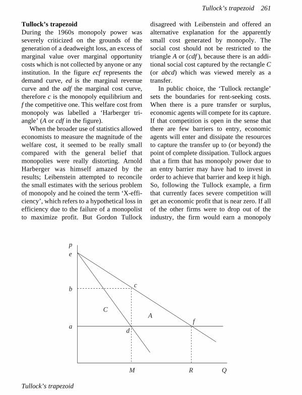
Tullock’s trapezoidDuring the 1960s monopoly power wasseverely criticized on the grounds of thegeneration of a deadweight loss, an excess ofmarginal value over marginal opportunitycosts which is not collected by anyone or anyinstitution. In the figure ecf represents thedemand curve, ed is the marginal revenuecurve and the adf the marginal cost curve,therefore c is the monopoly equilibrium andf the competitive one. This welfare cost frommonopoly was labelled a ‘Harberger tri-angle’ (A or cdf in the figure).

When the broader use of statistics allowedeconomists to measure the magnitude of thewelfare cost, it seemed to be really smallcompared with the general belief thatmonopolies were really distorting. ArnoldHarberger was himself amazed by theresults; Leibenstein attempted to reconcilethe small estimates with the serious problemof monopoly and he coined the term ‘X-effi-ciency’, which refers to a hypothetical loss inefficiency due to the failure of a monopolistto maximize profit. But Gordon Tullock

disagreed with Leibenstein and offered analternative explanation for the apparentlysmall cost generated by monopoly. Thesocial cost should not be restricted to thetriangle A or (cdf ), because there is an addi-tional social cost captured by the rectangle C(or abcd) which was viewed merely as atransfer.

In public choice, the ‘Tullock rectangle’sets the boundaries for rent-seeking costs.When there is a pure transfer or surplus,economic agents will compete for its capture.If that competition is open in the sense thatthere are few barriers to entry, economicagents will enter and dissipate the resourcesto capture the transfer up to (or beyond) thepoint of complete dissipation. Tullock arguesthat a firm that has monopoly power due toan entry barrier may have had to invest inorder to achieve that barrier and keep it high.So, following the Tullock example, a firmthat currently faces severe competition willget an economic profit that is near zero. If allof the other firms were to drop out of theindustry, the firm would earn a monopoly

Tullock’s trapezoid 261

CA

d

c

f

M R Q

p

e

b

a

Tullock’s trapezoid

power of, say, 100 monetary units. Assumingthat the firm could force the other firms out ofthe industry by investing 99 monetary units, itwould maximize profit by making the invest-ment. In the figure, its monopoly profit (Carea) would be 100, but proper accountancywould record a profit of only 1. So the greatermonopoly power would be associated withonly a small accounting profit, and it wouldexplain the low social cost due to monopoly.Thus, a ‘public finance view’ would considera social cost measured by a triangle (A), as the‘public choice view’ would consider a trape-zoid (A + C).

NURIA BADENES PLÁ

BibliographyTullock, G. (1967), ‘The welfare costs of tariffs, mon-

opolies and theft’, Western Economic Journal, 5,224–32.

Tullock, G. (1998), ‘Which rectangle?’, Public Choice,96, 405–10.

Tullock, G. (2003) ‘The origin of the rent-seekingconcept’, International Journal of Business andEconomics, 2 (1), 1–18.

See also: Harberger’s triangle.

Turgot–Smith theoremSaving decisions derived from frugality arethe source of investment and therefore ofeconomic growth. J.A. Schumpeter identi-fied the idea and its authors: French ministerand economist Anne Robert Jacques Turgot(1727–81) and Adam Smith. He attributed tothe former the analytic paternity and to thelatter the role of mere diffuser. After Smith,‘the theory was not only swallowed by thelarge majority of economists: it was swal-lowed hook, line, and sinker’ (Schumpeter,1954, pp. 323–6).

Turgot formulated the theory in hisReflections on the Production and Distribu-tion of Wealth (1766, LXXXI, LXXXII, CI,included in Groenewegen, 1977) and in thefinal part of the Observations on a Paper by Saint-Pèravy (1767, also included in

Groenewegen, 1977). His notions on savingand investment are part of a new capitaltheory that generalized François Quesnay’sanalysis of agricultural advances to allbranches of economic activity. In oppositionto the predominant view according to whichmoney not spent on consumption would leakout of the circular flow, Turgot argues thatsavings, accumulated in the form of money,would be invested in various kinds of capitalgoods, and so would return to circulationimmediately. He analyses five uses of thesaved funds: investing in agriculture, manu-facturing or commercial enterprises, lendingat interest, and purchasing land. Each ofthese provides a different but interrelatedprofitability, and an equilibrium position isachieved through the competitive processand the mobility of capital. Turgot excludeshoarding for its irrationality (lack of prof-itability) and because money was mainly amedium of exchange.

Adam Smith picked up Turgot’s thesesand in the Wealth of Nations (1776, bk II, ch.3) he developed his own doctrine on thedeterminant role of frugality and saving incapital accumulation. Smith’s most cele-brated and influential formulation of thetheorem is: ‘What is annually saved is asregularly consumed as what is annuallyspent, and nearly in the same time too; but itis consumed by a different set of people’(1776, p. 337). This was not accuratebecause it blurred the difference betweenconsumption and investment. But whatSmith meant was that investment results inincome payments, which in turn are spent onconsumption. Also excluding the hoardingpossibility, the Smithian dictum of ‘saving isspending’ was dominant among classical andneoclassical economists, but met with thecriticisms of Malthus, Sismondi, Marx,Keynes and their followers.

VICENT LLOMBART

262 Turgot–Smith theorem

BibliographyGroenewegen, Peter D. (1977), The Economics of A.R.J.

Turgot, The Hague: Martinus Nijhoff.Schumpeter, Joseph A. (1954), History of Economic

Analysis, London: George Allen & Unwin.

Smith, Adam (1776), An Inquiry into the Nature andCauses of the Wealth of Nations, 2 vols, reprinted1976, ed. R.H. Campbell and A.S. Skinner, Oxford:Clarendon Press.

See also: Say’s law.

Turgot–Smith theorem 263

Veblen effect goodIn his Theory of the Leisure Class (1899),Thorstein Veblen (1857–1929) developedthe theory of ‘conspicuous consumption’.The wealthy ‘leisure class’ made a lot ofconspicuous expenditure as a way to show itsstatus. In American culture, with classdistinctions blurred, this pattern is imitatedby the middle and lower classes. Then ‘pecu-niary emulation’ becomes the explanation ofconsumer behaviour, and not neoclassicaldemand theory, which Veblen thought unre-alistic.

Neoclassical economics has abstractedthis sociological and cultural explanation forconsumption – the very formation of tastesand consumption patterns – and developed itas a particular case in which the utility we getfrom a commodity is derived not only fromits intrinsic or instrumental qualities, butfrom the price we pay for it. This is called the‘Veblen effect’ and was formally presentedby Leibenstein in 1950. In order to know theeffects that conspicuous consumption has onthe demand function, we separate the effectof a change in price into two effects: the price effect and the ‘Veblen effect’.Previously we divided the price of the goodinto two categories: the real price, the moneywe pay for the good in the market, and the‘conspicuous price’, the price other peoplethink we have paid for the commodity.Traditionally it is thought that fashion cloth-ing, fashion products, fancy cars or evendiamonds are in demand as a means ofsignalling consumer wealth. If there is adifference between the two prices, the result-ing possible equilibria may yield an upward-sloping Veblenian demand curve, an excep-tion similar to Giffen goods but with a verydifferent explanation. In this way we use the

Veblen explanation for consumption withinthe neoclassical framework of microeconom-ics, but only for some particular kind ofgoods.

MANUEL SANTOS-REDONDO

BibliographyLeibenstein, H. (1950), ‘Bandwagon, snob and Veblen

effects in the theory of consumers’ demand’,Quarterly Journal of Economics, 64, 183–207;reprinted in W. Breit and H.M. Hochman (eds)(1971), Readings in Microeconomics, 2nd edn, NewYork: Holt, Rinehart and Winston, pp. 115–16.

Veblen, Thorstein ([1899] 1965), The Theory of theLeisure Class, New York: Augustus M. Kelley, pp.68–101.

Verdoorn’s lawDutch economist Petrus Johannes Verdoorn(1911–82) wrote in 1949 an article (pub-lished in Italian) that acquired fame onlyafter 20 years. He studied the relationshipbetween labour productivity and outputduring the inter-war period, using data of 15countries and different industrial sectors, andfound a close connection between the growthof productivity and the growth of industrialoutput. This empirical observation is thebasis of Verdoorn’s law, which says thatproduction growth causes productivitygrowth. Verdoorn explained his results asfollows: ‘Given that a further division oflabour only comes about through increases inthe volume of production; therefore theexpansion of production creates the possibil-ity of further rationalisation which has thesame effect as mechanisation’ (1949, 1993,p. 59).

Increasing returns to scale and technicalprogress, then, are the bases of Verdoorn’slaw: the expansion of production leads to theinvention of new manufacturing methods,

264

V

increasing productivity. Nicholas Kaldor(1966) was the first to point out the import-ance of Verdoorn’s work, and began to use itin his research. This is why this law is alsoknown as the Kaldor–Verdoorn law.

JOSÉ M. ORTIZ-VILLAJOS

BibliographyBoulier, B.L. (1984), ‘What lies behind Verdoorn’s

law?’, Oxford Economic Papers, 36 (2), 259–67.Kaldor, N. (1966), Causes of the Slow Rate of Economic

Growth of the United Kingdom, Cambridge:Cambridge University Press.

Verdoorn, P.J. (1949), ‘Fattori che regolano lo sviluppodella produttività del lavoro’, L’industria, I, 45–53;English version: ‘On the factors determining thegrowth of labour productivity’, in L. Pasinetti (ed.)(1993), Italian Economic Papers, II, Bologna: IlMulino and Oxford University Press, pp. 59–68.

Verdoorn, P.J. (1980), ‘Verdoorn’s law in retrospect: acomment’, Economic Journal, 90, 382–5.

See also: Kaldor’s growth laws.

Vickrey auctionWilliam Vickrey (1914–96) was awarded theNobel Prize in 1996 (jointly with James A.Mirrlees) for his fundamental contribution tothe economic theory of incentives underasymmetric information. His main researchfocus was on the fields of auction theory andoptimal income taxation.

Two questions are central in the auctionliterature. Which type of auction is betterfrom the seller’s point of view, and doauctions introduce distortions in the alloca-tion of objects so that they are not alwayssold to the person with the highest valuation?

Vickrey attached particular importance tothe second price auction (often referred to asthe Vickrey auction). In this kind of auction,the object is sold to the highest bidder whoonly pays the next highest price offered (the‘second price’). This mechanism leads indi-viduals to state bids equal to their true valu-ation of the object. Hence the object goes tothe person that values it the most (the bid isefficient even with private information), andthis person pays the social opportunity costwhich is the second price. Vickrey madeanother crucial contribution to the formal-ization of auctions: the revenue equivalenttheorem. Comparing second price and firstprice (where the winner pays his/her bid)auctions when the participants are risk-neutral and the individual valuations areindependent drawings from the same distri-bution, Vickrey proved that the two types ofauction are equivalent: the person with thehighest valuation obtains the object, and theexpected revenue is the same in bothauctions.

The game-theoretical approach proposedby Vickrey still has a central role in auctiontheory and in the design of resource alloca-tion mechanisms aimed at providing sociallydesirable incentives.

DAVID PÉREZ-CASTRILLO

BibliographyVickrey, W. (1961), ‘Counterspeculation, auctions and

competitive sealed tenders’, Journal of Finance, 16,8–37.

Vickrey auction 265

Wagner’s lawThe ‘law of increasing expansion of publicand particularly state activities’, known as‘Wagner’s law’, was formulated by Germaneconomist Adolf Wagner (1835–1917) in1883 and developed in other writings until1911. This law was just the result of empiri-cal observation in progressive countries, atleast in Western Europe: the expansion ofstate expenditure in absolute terms and as apercentage of national income. Wagnerincluded in this rule not only central and localgovernments but public enterprises as well.

‘Its explanation, justification and cause isthe pressure for social progress and the result-ing changes in the relative spheres of privateand public economy, especially compulsorypublic economy’ (Wagner, 1883, 1958, pp.9–10). Although many authors think thatWagner was only discussing the nineteenthcentury and not future events, much of theliterature applied and tested his law, withcontroversial results, during the twentiethcentury.

Linking increased public expenditure toideas such as progressive countries, socialpressure and ‘new’ public services (not onlyto the traditional services of defence, law andorder), Wagner seems to be conceiving thefuture in similar terms to what he hadobserved. But he recognized that there mustbe a limit to the expansion of the publicsector due to financial difficulties, sincefiscal requirements imply expenditure inhousehold budgets.

JUAN A. GIMENO

BibliographyGemmel, N. (1993), ‘Wagner’s law and Musgrave’s

hypotheses’, in N. Gemmel (ed.), The Growth of the

Public Sector, Aldershot, UK and Brookfield, US:Edward Elgar, pp. 103–20.

Peacock, A. and A. Scott (2000), ‘The curious attractionof Wagner’s law’, Public Choice, 102, 1–17.

Wagner, A. (1883, 1890), Finanzwissenschaft (2nd and3rd edns), partly reprinted in R.A. Musgrave andA.T. Peacock (eds) (1958), Classics in the Theory ofPublic Finance, London: Macmillan, pp. 1–15.

Wald testThe Wald test, or Wald method, is used totest a set of (linear or non-linear) restrictionson a parameter vector q (q × 1), say, forwhich we have available an asymptoticallynormal estimator. Wald (1943) developedthe method in the context of maximum like-lihood (ML) estimation, but nowadays it isused in general estimation settings.

Let q be an estimator of q based on samplesize n, such that

��n(q – q) d→N(0, S), (1)

where d→denotes convergence in distributionas n → ∞, and N(0, S) is a (multivariate)normal distribution of mean zero and vari-ance–covariance matrix S (which may dependon q). Assume we have a consistent estima-tor S fl of S.

Consider the null hypothesis H0: h(q) = 0,where h(.) is a continuously differentiable r ×1 (r ≤ q) vector-valued function of q, and thealternative hypothesis H1: h(q) ≠ 0. TheWald test statistic for H0 is

W = nh �{H S fl Hfl �}–1h (2)

where h = h(q) and H is the (r × q) matrix ofpartial derivatives H = ∂h(q)/∂q evaluated atq. In the classical set-up, H is a regular matrix(as a function of q) and of full column rank,and S is non-singular (thus, HS fl H fl� has regu-lar inverse). Under H0, W is asymptotically

266

W

chi-square distributed with r degrees of free-dom; that is, W d

→ c2r; hence the (asymptotic

a-level (Wald) test of H0 rejects H0 when W> ca,r, where ca,r is the (1 – a )100th percentile of the c2

r (i.e., P[c2r > ca,r] = a). The

value ca,r is called the ‘critical value’ of thetest.

A very simple example of a Wald testarises when q is scalar (that is, q = 1) and H0:q = q0 (that is, h(q) = q – q0). In this simplesetting,

(q – q0) 2

W = n(q – q0)2/s2 = (———),s/��n

where s/��n is (asymptotically) the standarddeviation of q; in this case, W is the square ofa ‘standardized difference’ or, simply, thesquare of a ‘z-test’.

A popular example of the Wald test arisesin the regression setting y = Xb + ∈ , wherey(n × 1) and X (n × K) correspond to thevalues of the dependent and independentvariables, respectively, b(K × l) is the vectorof regression coefficients, and ∈ (n × l) is thevector of disturbances. Let H0: Ab = a, whereA (r × K) and a (r × l) are a matrix and vector,respectively, of known coefficients. Assume,for simplicity of exposition, var(∈ ) = s 2Inand A of full rank. It is well known that b =(X�X)1X�y, the OLS estimator of b, satisfies��b(b – b) d→N(0, S), where S = s2{n–1X�X}–1;thus, W of (2) is W = (Ab – a)�{s2A(X�X)–1

A�}–1(Ab – a), where s2 is a consistent esti-mate of s2.

When s2 is the usual unbiased estimate of s2, s2 = s2 = ∑n

i e2i /(n – K), it can be seen that

F = W/r is the classical F-test for H0. Undernormality of ∈ , F is distributed exactly (forall sample sizes!) as an F-distribution with rand n – K degrees of freedom. In fact when q= 1 and H0: q = q0, the equality W = rFexpresses then W (= F) is the square of thefamiliar t-test statistic (that is, the square ofthe ‘t-value’). Under normality and smallsamples, the F-test may give a more accurate

test than the (asymptotic) Wald test; for largesamples, however, both the F and Wald testare asymptotically equivalent (note that,owing to this equivalence, the F-test isasymptotically robust to non-normality).

In the non-standard case where H and S; Sare not of full rank, the Wald test still appliesprovided that (a) in (2) we replace the regu-lar inverse with the Moore-Penrose inverse;(b) we use as degrees of freedom of the test r= r (H S H �); and (c) we assume r = r{HflSflHfl �}= r{HSH �} with probability 1, as n→ ∞. (Here, r(.) denotes rank of the matrix).

For a fixed alternative that does notbelong to H0, the asymptotic distribution ofW is degenerate. However, under a sequenceof local alternatives (see Stroud, 1972) of theform H1: ����nh(q) = � where �(r × 1) is a fixvector, it holds W d

→c2(r, l) where c2(r, l) isa non-central chi-square distribution of rdegrees of freedom and non-centrality para-meter l = ��{H S H�}–1�. Such a non-degen-erate asymptotic distribution of W has beenproved useful for approximating the powerof the test (that is, the probability of rejectingH0 when in fact H0 does not hold) when thealternatives of interest are not too deviantfrom H0. (In the non-standard set-up of Ssingular, � need is assumed to be in thecolumn space of H S H�).

The Wald test is asymptotically equiva-lent to the other two classical large-sampletests, the log-likelihood ratio (LR) test andthe Lagrange multiplier (LM) (also calledScore) test.

For non-linear restrictions, the Wald testhas the disadvantage of not being invariant tore-parameterization of the null hypothesisH0. Consider, for example, q = (q1, q2)� andthe restriction H0: q1,q2 = 1; an alternativeexpression for this restriction is H0: q1 =1/q2. In fact, these two alternative parameter-izations of H0 can be seen to yield differentvalues for W, hence possibly differentconclusions of the test.

A consistent estimate S fl of S is needed to

Wald test 267

construct the Wald test. When alternativeestimates for S are available, the issue can beposed of which of them is more adequate.For example, in the context of ML estimationS fl can be based either on the observed infor-mation (the Hessian) or on the expectedinformation matrices, with this choice havingbeen reported to affect substantially the sizeof the Wald test.

ALBERT SATORRA

BibliographyStroud, T.W.F. (1972), ‘Fixed alternatives and Wald

formulation of the non-central asymptotic behaviorof the likelihood ratio statistic’, Annals ofMathematical Statistics, 43, 447–54.

Wald, A. (1943), ‘Tests of statistical hypothesesconcerning several parameters when the number ofobservations is large’, Transactions of the AmericanMathematical Society, 54 (3), 426–82.

Walras’s auctioneer and tâtonnementThe most striking thing about Walras’sauctioneer is not that, as with many othercharacters that have shaped our world or ourminds, nobody has ever seen him but the factthat Walras himself never knew of his exist-ence. Walras’s auctioneer was an inventionthat saw the light some decades after thedeath of his alleged inventor.

In his Élements (1874), Walras estab-lished the foundations of general equilibriumtheory, including the definition of equilib-rium prices as the solution to a system ofequations, each representing the balance ofsupply and demand in one market. But howwere these prices implemented? Walras wasadamant in seeking an answer to what eventoday is perhaps the most important of theopen questions in economics. He argued that,in real markets, a tâtonnement (groping)process would lead to them: prices below theequilibrium levels would render supplyinsufficient to meet demands, and vice versa.The markets would then grope until theyfound a resting place at equilibrium prices.

One shortcoming of this description of the

workings of real markets is that consistencyrequires that trade materialize only after theright prices are found. In well-organizedmarkets, like some financial markets, this isguaranteed. However, in more decentralizedmarkets, individual trades cannot wait for all markets to clear. Faced with this diffi-culty, Walras’s tâtonnement became moreand more either a way to prove the existenceof equilibrium prices or an ideal way to conceive gravitation towards them. Itbecame more a convenient parable to explainhow prices could be found than a descriptionof how prices were found. And it is in thiscontext of diminished ambition that theWalrasian auctioneer was brought into thehistory of economic thought, to the scarcelyheroic destiny of leading this gropingprocess, quoting and adjusting imaginaryprices in the search for the equilibriumfinale.

ROBERTO BURGUET

BibliographyWalras, L.M.E. (1874–7), Eléments d’économie poli-

tique pure, Lausanne: Rouge; definitive edn (1926),Paris: F. Pichon.

Walras’s lawThe idea that markets are not isolated but thatthere is an interrelationship among themarkets for different commodities is thecentral contribution of Léon Walras (1834–1910) to economic science. As an outcomeof this idea, Walras’s law emerges.

In a Walrasian economic model, anytrader must have a feasible and viable netconsumption plan; that is, the trader’sdemand for any commodity implies the offerof commodities in exchange for it. For eachtrader the total value (in all markets) of theirplanned supply must exactly equal the totalvalue (in all markets) of their planneddemand. That relation shows that the indi-vidual budget equation (constraint) is met.

268 Walras’s auctioneer and tâtonnement

Considering this fact, the relationshipbetween the aggregation of those individualbudget equations for all traders can beobserved. By aggregating, the value of thetotal demand of all traders, summed over allmarkets, has to be equal to the sum of thevalue of the total supply by all traders in allmarkets. If we now look at this aggregatedrelationship, it can be said that the aggre-gated value of the net demanded quantities(total demand minus total supply, called‘demand excess’ in the literature) has to beequal to zero. In other words, this reflects thefact that, at whatever level the prices aneconomy are, the sum of the individual posi-tive and negative quantities in all markets isidentically zero, and this is true whether allmarkets are in (general) equilibrium or not.This relationship is known as Walras’s law.

To be more precise, Walras’s law can bedefined as an expression of the interdepen-dence among the excess demand equations ofa general equilibrium system that arises fromthe budget constraint (see Patinkin, 1987).

Walras’s law has several fundamentalimplications: (i) if there is positive excess of demand in one market then there must be, corresponding to this, negative excessdemand in another market; (ii) it is possibleto have equilibrium without clearance of allmarkets explicitly taking into account all thesimultaneous interactions and interdepen-dences that exist among markets in the econ-omy. As a main conclusion of (i) and (ii), itcan be said, first, that the equilibrium condi-tions in N markets are not independent, thatis, there is an interrelationship amongmarkets. Suppose we have N markets in theeconomy. If each trader’s budget constraintholds with equality and N – 1 markets clear,then the Nth market clears as well. So it ispossible to neglect one of the market-clear-ing conditions since it will be automaticallysatisfied. Second, given that the markets areinterrelated, either all markets are in equilib-rium, or more than one is in disequilibrium,

but it is not possible to find the situationwhere only one market is in disequilibrium.

ANA LOZANO VIVAS

BibliographyPatinkin, D. (1987), ‘Walras law’, The New Palgrave, A

Dictionary of Economics, London: Macmillan, vol.4, pp. 864–8.

Walras, L.M.E. (1874–7), Élements d’économie poli-tique pure, Lausanne: Rouge; definitive edn (1926),Paris: F. Pichon.

See also: Say’s law.

Weber–Fechner lawThe works of German physiologist ErnstHeinrich Weber (1795–1878) and of Germanpsychologist Gustav Theodor Fechner (1801–87) may be considered as landmarks inexperimental psychology. They both tried torelate the degree of response or sensation ofa sense organ to the intensity of the stimulus.The psychophysiological law bearing theirnames asserts that equal increments of sensa-tion are associated with equal increments ofthe logarithm of the stimulus, or that the justnoticeable difference in any sensation resultsfrom a change in the stimulus with a constantratio to the value of the stimulus (Blaug,1996, p. 318).

By the time Weber (1851) and Fechner(1860) published their findings, politicaleconomy was to some extent becomingready to welcome every bit of evidencerelating to human perception and response toseveral economic situations. As a conse-quence, this law was likely to be coupledwith the analysis of the consequences of achange in the available quantities of acommodity (the idea that equal incrementsof a good yield diminishing increments ofutility, the analysis of consumers’ responsesto changes in prices, the tendency of indi-viduals to evaluate price differences relativeto the level of the initial price, or to theanalysis of the different attitudes towards

Weber–Fechner law 269

risk), the increment in gratification dimin-ishing with the increase of a man’s totalwealth.

William Stanley Jevons first linked theWeber–Fechner law to economic analysis,by giving a supposedly sound psychophysio-logical foundation to the idea that commodi-ties are valued and exchanged according totheir perceived marginal utility.

ANTÓNIO ALMODOVAR

BibliographyBlaug, Mark (1996), Economic Theory in Retrospect,

5th edn, Cambridge: Cambridge University Press.Schumpeter, J.A. (1954), History of Economic Analysis,

New York: Oxford University Press, p. 1058.

Weibull distributionThis is a popular probability distribution forduration data. It was developed by WallodiWeibull (1939), a Swedish engineer, in aseminal paper on the strength of materials.The use of this distribution to adjust data didnot attract much attention until the 1950s,when the success of the method with verysmall samples in reliability analysis couldnot be ignored.

Nowadays the Weibull distribution iswidely used in many areas to modelprocesses duration, especially in engineer-ing, biomedical sciences and economics.Applications in economics include the esti-mation of the duration of unemployment,firms’ lifetime, investment decision makingand durable products.

Let T be a nonnegative random variablerepresenting the duration of a process. TheWeibull probability density function is ƒ(t) =lb(lt)b–1 exp{–(lt)b}, t > 0 where l > 0 andb > 0 are parameters. The exponential distri-bution is a special case of the Weibull distri-bution with b = 1.

The success of Weibull distribution toadjust data is due to its versatility. Dependingon the value of the parameters, the Weibulldistribution can model a variety of life behav-

iours. This property can be easily shownusing the hazard function, h(t). The hazardfunction specifies the instantaneous rate ofdeath, failure or end of a process, at time t,given that the individual survives up to timet:

Pr(t ≤ T ≤ t + Dt | T ≥ t)h(t) = lim ——————————.

Dt→0 Dt

The Weibull distribution’s hazard func-tion is h(t) = lb(lt)b–1. This function isincreasing if b > 1, decreasing if b < 1 andconstant if b = 1. Thus the model is very flex-ible and provides a good description of manytypes of duration data. This versatility is thereason for the wide use of Weibull distribu-tion in many areas.

TERESA VILLAGARCÍA

BibliographyWeibull, W. (1939), ‘A statistical theory of the strength

of materials’, Ing. Vetenskaps Akad. Handl., 151,1–45.

Weierstrass extreme value theoremIn its simplest version, this theorem statesthat every continuous real valued function fdefined on a closed interval of the real line(that is: f: [a, b] → R) attains its extremevalues on that set. In other words: there existx1, x2 ∈ [a, b] such that f(x1) ≤ f (x) ≤ f(x2) forevery x ∈ [a, b].

Such a theorem was proved in the 1860sby the German mathematician Karl TheodorWilhelm Weierstrass (1815–97), whose stan-dards of rigour strongly affected the future ofmathematics. A remarkable example of hisachievements is the discovering in 1861 of areal function that, although continuous, hadno derivative at any point. Analysts whodepended heavily upon intuition wereastounded by this counterintuitive function.

Karl Weierstrass is known as the Father ofModern Analysis. His theorem has many

270 Weibull distribution

generalizations of an analytical, topologicalor ordinal nature. For instance, it is true that

1. Every continuous real valued function fdefined on a non-empty closed andbounded subset of the n-dimensionalspace Rn attains its extreme values onthat set.

2. Every continuous real valued function fdefined on a non-empty compact topo-logical space X attains its extreme valueson that set.

3. For every continuous total preorder �defined on a non-empty compact set Xthere exist elements x1, x2 ∈ X such thatx1 � x � x2 for an y x ∈ X.

Weierstrass’s extreme value theorem hasmany applications in mathematical econom-ics. For instance, it is often used in situationsin which it is important to guarantee the exist-ence of optimal points related to preferencerelations or utility functions of an economicagent.

ESTEBAN INDURÁIN

BibliographyPoincaré, Henry (1899), ‘L’œuvre mathématique de

Weierstrass’, Acta Mathematica, 22, 1–18.

White testThis is a general test for heteroskedasticitythat, in contrast to other tests, does notrequire the specification of the nature of theheteroskedasticity. This test can only beapplied to large samples.

The null hypothesis is that the sample vari-ance of least squares residuals (Var u = s2 I)is homoskedastical H0: s2

i = s2I for all i, andthe alternative, that variance is heteroskedas-tical (Var u = s2W�W ≠ I) Hl: s

2i ≠ s2.

The test is based on the comparison of thevariance–covariance matrix of the ordinaryleast squares (OLS) estimators of the model(b) under the null hypothesis,

Var b = s2(X�X)–1,

and under heteroskedasticity,

Var b = s2(X�X)–1 (X�WX) (X�X)–1,

When the null hypothesis is true, the two estimated variance–covariance matricesshould, in large samples, differ only becauseof sampling fluctuations. White has deviseda statistical test based on this observation.Heteroskedasticity, if it exists, can be causedby the regressors from the equation beingestimated (Xi), their squares (Xi

2) and thecross-products of every pair of regressors.

White’s test can be computed as T*R2,where T is the sample size and R2 comesfrom an auxiliary regression of the square ofOLS residuals (ût

2), on a constant, the regres-sors from the original equation being esti-mated (Xi), their squares (Xi

2) and thecross-products of every pair of regressors.

In general, under the null of homoskedas-ticity, the statistic of White is asymptoticallydistributed as chi-squared T * R2d

→c2(q) with

q degrees of freedom, where q is the numberof independent variables in the auxiliaryregression excluding the constant. If thisstatistic is not significant, then ût

2 is notrelated to Xi and Xi

2 and cross-products andwe cannot reject the hypothesis that varianceis constant.

NICOLÁS CARRASCO

BibliographyWhite, H. (1980), ‘A heteroskedastic-consistent covari-

ance matrix estimator and a direct test forheteroskedasticity’, Econometrica, 48, 817–38.

Wicksell effectThis notion refers to the change in the valueof capital associated with a change in the rateof interest or rate of profit. Two effects aredistinguished: a price and a real effect. Whilethe latter involves a change of technique, the

Wicksell effect 271

former refers to a given technique (to a givenset of capital goods). A negative price effectresults when, for some range of the rate ofprofit, a higher value of capital (per person)is associated with a higher rate of profit. Apositive price effect results when a highervalue of capital is associated with a lowerrate of profit. A neutral price effect resultswhen the value of capital is invariant tochanges in the rate of profit. As the realeffect involves a choice of technique, theanalysis focuses on switch points. A negativereal effect results when the techniqueadopted at lower rates of profit has a value ofcapital per person lower than the techniqueadopted at higher rates of profit. A positivereal effect results when the techniqueadopted at lower rates of profit has a value ofcapital per person higher than the techniqueadopted at a higher rate of profit.

Although the term was introduced by Uhr(1951), the notion was fully developed,following Robinson, during the ‘Cambridgecontroversy in the theory of capital’. In thiscontext, three main issues should be singledout: the specification of the endowment ofcapital as a value magnitude, the determin-ation of the rate of profit by the marginalproduct of capital, and the inverse monotonicrelationship between the rate of profit and the‘quantity’ of capital per person.

Knut Wicksell (1851–1926) himself castsdoubt on the specification of the value ofcapital, along with the physical quantities oflabour and land, as part of the data of thesystem. ‘Capital’ is but a set of heteroge-neous capital goods. Therefore, unlike labourand land, which ‘are measured each in termsof its own technical unit . . . capital . . . isreckoned . . . as a sum of exchange value’(Wicksell, 1901, 1934, p. 49). But capitalgoods are themselves produced commoditiesand, as such, their ‘costs of productioninclude capital and interest’; thus, ‘to derivethe value of capital-goods from their owncost of production or reproduction’ would

imply ‘arguing in a circle’ (ibid., p. 149).Wicksell further argued that the marginalproduct of social capital is always less thanthe rate of interest (profit) (cf. ibid. p. 180).This is due to the revaluation of capitalbrought about by the fall in the rate of profitand the rise of the wage rate consequent uponan addition to existing capital.

The central issue at stake is the depen-dence of prices on the rate of profit, whichwas already well known to Ricardo andMarx. Sraffa (1960) provides a definitiveanalysis of that dependence: prices areinvariant to changes in the rate of profit onlyin the special case in which the proportionsof labour to means of production are uniformin all industries. From the standpoint of thevalue of capital, it is only in this case that aneutral-price Wicksell effect is obtained. Inthe general case of non-uniform ‘propor-tions’, variations in the rate of profit ‘giverise to complicated patterns of price-move-ments with several ups and downs’ (ibid., p.37). Indeed, these price variations apply tocapital goods as to any produced commodity.Thus, as the rate of profit rises, the value ofcapital, of given capital goods, ‘may rise or itmay fall, or it may even alternate in risingand falling’ (ibid., p. 15). So both negativeand positive-price Wicksell effects areobtained and they may even alternate. Itfollows that neither the value of capital northe capital intensity of production can beascertained but for a previously specified rateof profit. As Sraffa argues, ‘the reversals inthe direction of the movement of relativeprices, in the face of unchanged methods ofproduction, cannot be reconciled with anynotion of capital as a measurable quantityindependent of distribution and prices’.Indeed, this being so, it seems difficult tosustain the argument that the marginal prod-uct of capital determines the rate of profit.

Sraffa’s analysis of prices in terms of their‘reduction to dated quantities of labour’ canbe taken as applying to the variations in the

272 Wicksell effect

relative cost of two alternative techniques.The analysis then shows the possibility ofmultiple switches between techniques. Thisimplies that techniques cannot be orderedtransitively in terms of their capital intensi-ties (or of the rate of profit). While thereswitching of techniques involves negativereal Wicksell effects (‘reverse capital deep-ening’), its non-existence does not precludethem. And negative real effects do indeedrule out the inverse monotonic relationshipbetween the rate of profit and capital perperson.

CARLOS J. RICOY

BibliographyFerguson, C.E. and D.L. Hooks (1971), ‘The Wicksell

effect in Wicksell and in modern capital theory’,History of Political Economy, 3, 353–72.

Sraffa, P. (1960), Production of Commodities by Meansof Commodities, Cambridge: Cambridge UniversityPress.

Uhr, C.G. (1951), ‘Knut Wicksell, a centennial evalu-ation’, American Economic Review, 41, 829–60.

Wicksell, K. (1893), Über Wert, Kapital and Rente,English edn (1954), Value, Capital and Rent,London: Allen & Unwin.

Wicksell, K. (1901), Föreläsningar i nationalekonomi.Häft I, English edn (1934), Lectures on PoliticalEconomy. Volume I: General Theory, London:Routledge & Kegan Paul.

See also: Pasinetti’s paradox, Sraffa’s model.

Wicksell’s benefit principle for the distribution of tax burdenAccording to this principle, the taxpayer’scontributions should have a fiscal burdenequivalent to the benefits received from thepublic expenditure, which implies a quidpro quo relation between expenditure andtaxes.

The benefit principle solves at the sametime the problem of tax distribution and theestablishment of public expenditure. Withina society respectful of individual freedom,the benefit principle guarantees that no onewill pay taxes on services or public activitieshe or she does not want.

A problem related to the benefit principleis that it does not contemplate the jointconsumption of public goods, which allowsthe taxpayer to hide his real preferences forthe public goods and to consume them with-out paying.

In this context, Knut Wicksell’s (1851–1926) contribution has two main aspects. Onthe one hand, it stresses the political essenceof the taxation problem. A true revelation ofpreferences is unlikely, as it is that individu-als will voluntarily make the sacrifice oftaxation equal to the marginal benefit of theexpenditure.

Wicksell defends the principle of (approxi-mate) unanimity and voluntary consent intaxation. State activity can be of generalusefulness, the next step being to weigh theexpected utility against the sacrifice of taxa-tion.

This decision should not neglect the interest of any group and unanimity is therule that ensures this. Moreover, unanimity is equivalent to the veto power, and for this reason Wicksell proposes approximateunanimity as the decision rule. On the otherhand, Wicksell points out an importantaspect of public activity which is differentfrom the first one, such as achieving a justincome distribution, because ‘it is clear thatjustice in taxation presupposes justice in theexisting distribution of property and income’(Wicksell, 1896, p. 108).

This distinction between the problem ofachieving a just distribution of income andthe different problem of assignment of thecosts of public services is surely Wicksell’smain contribution to public economics.

CARLOS MONASTERIO

BibliographyMusgrave, R. (1959), The Theory of Public Finance,

New York: McGraw-Hill.Wicksell, K. (1896), ‘Ein neues Prinzip der gerechten

Besteuerng’, Finanztheoretische Untersuchungen,Jena. English trans. J.M. Buchanan,‘A new principle

Wicksell’s benefit principle for the distribution of tax burden 273

of just taxation’, in R. Musgrave and A. Peacock(eds) (1967), Classics in the Theory of PublicFinance, New York: St. Martin’s Press, pp. 72–118.

Wicksell’s cumulative processSwedish economist Johan Gustav KnutWicksell (1851–1926) first developed hisanalysis of the cumulative process inGeldzins und Güterpreise (Interest andPrices), published in 1898. After presentinghis capital and monetary theory, he analysedthe relation between interest rates and pricesmovements. Money (or bank) and natural(or real) rates of interest are two differentvariables in his theory. The first is deter-mined in the long period by the second, butthe current level of both variables need notbe the same. If there is a divergence betweenmoney and natural rate of interest, pricesmove in a cumulative process (Wicksell,1898, pp. 87–102, pp. 134–56 in the Englishversion).

Wicksell’s proposal must be understoodin the context of the monetary discussionslinked to the secular increase of prices in thesecond half of the nineteenth century. Whilein his opinion classical quantitative theorywas basically correct, he believed it wasunable to explain price movements in a crediteconomy. Nevertheless, the practical use ofWicksell’s theory is finally limited becauseof the nature of the key variable: the naturalrate that refers to an expected profit and notto a current value (Jonung, 1979, pp.168–70).

Wicksell thus presented a brief descrip-tion of his theory: ‘If, other things remainingthe same, the leading banks of the worldwere to lower their rate of interest, say 1 percent below its originary level, and keep it sofor some years, then the prices of allcommodities would rise and rise without anylimit whatever; on the contrary, if the leadingbanks were to raise their rate of interest, say1 per cent above its normal level, and keep itso for some years, then all prices would fall

and fall and fall without limit except zero’(Wicksell, 1907, p. 213).

This process takes place as follows. Let usassume a pure credit economy; the moneysupply is thus endogenous, in full equilib-rium, that is, in a situation of full employ-ment and monetary equilibrium. Thensuppose that, as a consequence of technicalprogress, a change in productivity takesplace. Then a divergence between the naturalrate and the bank rate of interest (in > im)develops as the latter remains at its originallevel. As a consequence, entrepreneurs havea surplus profit and their first intention willbe to increase the level of production. Theentrepreneur’s attempt to expand productionwill result in increased prices. In a situationof full employment, this individual strategyto expand production is ruled out in aggre-gate terms. The increase of the demand forinputs leads to a higher level of prices. Inputowners have a higher income because of thenew price level and they increase theirdemand of consumer goods. Consequently,this action leads to a higher level of prices ofconsumer goods. At this point, entrepreneursagain find a surplus profit as at the beginningof this process.

As long as the banking system does notchange the rate of interest policy, the diver-gence between market and natural rate ofinterest will remain, and the process willcontinue indefinitely. Conversely, if, at thebeginning of the process, the natural rate ofinterest happens to be below the money rate(in < im) a downward cumulative processwould ensue; the process develops becausewages are flexible enough to maintain fullemployment.

Of course, as the cumulative process,upward or downward, develops as a conse-quence of a divergence between natural andmoney rates of interest, any economic factwhich affects both rates can be the cause ofthe beginning of the process. Particularlyrelevant in this regard is the role of monetary

274 Wicksell’s cumulative process

policy in price stabilization. Insofar as mon-etary policy is the first determinant of themoney rate of interest, this should beadjusted to any change in the natural rate.

The later theoretical influence of theWicksellian cumulative process was espec-ially important in Sweden. In the 1930s, itbecame the theoretical background of thedynamic theory of Wicksell’s followers inthe Stockholm School, mainly Myrdal andLindahl. Later it also became a reference inthe research on the relation between mon-etary theory and Walrasian value theory(Patinkin, 1952).

JOSÉ FRANCISCO TEIXEIRA

BibliographyJonung, Lars (1979), ‘Knut Wicksell and Gustav Cassel

on secular movements in prices’, Journal of Money,Credit and Banking, 11 (2), 165–81.

Patinkin, Don (1952), ‘Wicksell’s “Cumulative Process” ’,Economic Journal, 62, 835–47.

Uhr, C. (1960), Economic Doctrines of Knut Wicksell,Berkeley: University of California Press, pp.235–41.

Wicksell, J.G.K. (1898), Geldzins und Güterpreise:Eine Studie über den Tauschwert des Geldes bestim-menden Ursachen, Jena; English version (1936)Interest and Prices, London: Macmillan.

Wicksell, J.G.K. (1907), ‘The influence of the rate ofinterest on prices’, Economic Journal, 17, 213–20.

Wiener processSuppose that a particle moves along an axis.The particle suffers a displacement constantin magnitude but random in direction. TheWiener process can be viewed as the limit ofa sequence of such simple random walks.Assume that between times t and t + n – 1,the particle makes a small increment of sizen–1/2 forwards or backwards with the sameprobability, so that there are very many butvery small steps as time goes by. The charac-teristic function of this increment iscos(tn–1/2). Then, in the time interval of [0,h], the characteristic function of the particleposition (a sum of nh independent incre-ments) is cos(tn–1/2)nh. When the number n

goes to infinity, the limit distribution of theposition has the characteristic distributionexp(–t2h/2) which corresponds to the charac-teristic function of the centered Gaussiandistribution with variance h. This continuoustime process is the Wiener process, which isalso known as the standard Brownianmotion. The discovery of this process, in1828, is credited to Robert Brown, a botanistwho observed the random movement ofpollen grains under a microscope. AlbertEinstein in 1905 gave the first mathematicaldemonstration of the underlying normaldistribution by working with a collection ofpartial differential equations. However, itwas Norbert Wiener (1923) and later PaulLevy (1937–48) who described many of themathematical properties of this process,which has the following definition.

A Wiener process {W(t): t ≥ 0} is a stochas-tic process having: (i) continuous paths, (ii)stationary, independent increments, and (iii)W(t) normally distributed with mean 0 andvariance t. Each realization of this process is areal continuous function on {t ≥ 0} which canbe viewed as a ‘path’. However, it is impossi-ble to graph these sample paths because, withprobability one, W(t) is nowhere differentiable(path with infinite length between any twopoints). The independent increments require-ment means that, for each choice of times 0 ≤t0 < t1 < . . . <tk < ∞, the random variables W(t1)– W(t0),W(t2) – W(t1), . . ., W(tk) – W(tk–1) areindependent. The term ‘stationary increments’means that the distribution of the incrementW(t) – W(s) depends only on t – s. Finally,from (ii) and (iii), it follows that, for every t >s, the increment W(t) – W(s) has the samedistribution as W(t – s) – W(0) which isnormally distributed with mean 0 and variancet – s.

The behavior of the Wiener processbetween two time points can be described byits conditional distribution. From the previ-ous definition, it follows that, for any t > s >0, the conditional distribution of W(s) given

Wiener process 275

W(t) is normal with mean (s/t)W(t) and vari-ance s(t – s)/t. Note that W(t) is also Markov:given the current state W(s), the behavior ofthe process {W(t): t ≥ s} does not depend onthe past {W(u):u ≤ s}.

The Wiener process is a standardizedversion of a general Brownian motion andcan be generalized in various ways. Forinstance, the general Brownian motion on {t≥ 0} need not have W(0) = 0, but may have anon-zero ‘drift’ m, and has a ‘variance para-meter’ s2 that is not necessarily 1.

The Wiener process is valuable in manyfields, especially in finance because of itshighly irregular path sample and its assump-tion which is the same as assuming a unitroot in time-series analysis.

OLIVER NUÑEZ

BibliographyBrown, R. (1828), ‘A brief account of microscopical

observations made in the months of June, July, andAugust, 1827, on the particles contained in thepollen of plants; and on the general existence ofactive molecules in organic and inorganic bodies’,Philosophical Magazine, N.S. 4, 161–73.

Doob, J.L. (1953), Stochastic Processes, New York:John Wiley & Sons.

See also: Gaussian distribution.

Wiener–Khintchine theoremThis theorem is a classical result in spectralor Fourier analysis of time series. Thecentral feature of this analysis is the exist-ence of a spectrum by which the time seriesis decomposed into a linear combination ofsines and cosines. The spectrum, fromstatistical physics, is a display of the seriesat different frequencies, relating how manywave patterns pass by over a period of time.The power spectrum function of a timeseries is a real valued, non-negative func-tion evaluating the power of the time seriesat each frequency. The W–K theorem statesthat the power spectrum of a randomprocess is the Fourier transform of its auto-correlation function. The W–K relations

assert the complete equivalence of the auto-covariance function of the stochasticprocess and its spectral distribution func-tion. The spectral distribution function of aset of frequencies gives the amount ofpower in the harmonic components of thetime series with frequencies in the setconsidered. The W–K theorem is used prac-tically to extract hidden periodicities inseemingly random phenomena. From themathematical point of view, this is a partic-ular case of the convolution theorem, whichstates that the Fourier transform of theconvolution of two functions equals theproduct of the Fourier transforms.

ROSARIO ROMERA

BibliographyWiener, N. (1949), Extrapolation, Interpolation and

Smoothing of Stationary Time Series withEngineering Applications, Cambridge, MA.: TheMIT Press; New York: Wiley and Sons; London:Chapman & Hall.

See also: Fourier transform.

Wieser’s lawCoined by Italian economist MaffeoPantaeloni, this refers to what was to becalled the opportunity cost, also known asalternative cost, presented in 1876 byAustrian economist Friedrich von Wieser(1851–1926) and developed in his laterworks. Wieser was an early member of theAustrian School of Economics, andsucceeded the founder, Carl Menger, at theUniversity of Vienna, but did not share theclassical liberal stance upheld by virtually allof its members.

Although the idea of explaining valuesand costs in terms of forgone opportunities,one of the most widely used in economicsever since, had several antecedents –Cantillon, Thünen, Mill, Menger, Walras andothers, not to speak of the medieval lucrumcessans of Scholastic lawyers – Wieserformulated the equimarginal principle in

276 Wiener–Khintchine theorem

production, and defined cost explicitly assacrifice. In Social Economics he says:

In what does this sacrifice consist? What, forexample, is the cost to the producer of devotingcertain quantities of iron from his supply to themanufacture of some specifict product? Thesacrifice consists in the exclusion or limitationof possibilities by which other products mighthave been turned out, had the material not beendevoted to one particular product . . . It is thissacrifice that is predicated in the concept ofcosts: the costs of production or the quantitiesof cost-productive-means required for a givenproduct and thus withheld from other uses.

CARLOS RODRÍGUEZ BRAUN

BibliographyWieser, Friedrich von (1876), ‘On the relationship of

costs to value’, in I.M. Kirzner (ed.) (1994), Classicsin Austrian Economics, vol. 1, London: Pickering &Chatto, pp. 207–34.

Wieser, Friedrich von (1927), Social Economics firstpublished in German, (1914), London: George Allen& Unwin, pp. 99–100.

Williams’s fair innings argumentFirst defined by John Harris in 1985, thisargument of intergenerational equity in healthwas developed in 1997 by Alan Williams,professor of Economics at the University ofYork, and reflects the feeling that there is anumber of years broadly accepted as areasonable life span. According to this notion,those who do not attain the fair share of lifesuffer the injustice of being deprived of a fairinnings, and those who get more than theappropriate threshold enjoy a sort of bonusbeyond that which could be hoped for. Thefair innings argument implies that health careexpenditure, in a context of finite resources,should be directed at the young in preferenceto elderly people. Discrimination against theelderly dictated by efficiency objectivesshould, therefore, be reinforced in order toachieve intergenerational equity.

Williams claims that ‘age at death shouldbe no more than a first approximation’ in orderto inform priority setting in health care,

‘because the quality of a person’s life is impor-tant as well as its length’ (Williams, 1997, p.117). According to his view, the number ofquality-adjusted life-years an individual hasexperienced is relevant to allocating healthcare resources, and future gains should bedistributed so as to reduce inequalities in life-time expectations of health. Williams high-lights four characteristics of the fair inningsnotion: ‘firstly, it is outcome-based, notprocess-based or resource-based; secondly, itis about a person’s whole life-time experience,not about their state at any particular point intime; thirdly, it reflects an aversion to inequal-ity; and fourthly, it is quantifiable’ (ibid.). Thequantification of the fair innings notionrequires the computation of specific numericalweights reflecting the marginal social value ofhealth gains to different people.

ROSA MARÍA URBANOS GARRIDO

BibliographyHarris, J. (1985), The Value of Life, an Introduction to

Medical Ethics, London: Routledge & Kegan Paul.Williams, A. (1997), ‘Intergenerational equity: an

exploration of the “fair innings” argument’, HealthEconomics, 6, 117–32.

Wold’s decompositionHerman Ole Andreas Wold (1908–1992)proved in his doctoral dissertation a decom-position theorem that became a fundamentalresult in probability theory. It states that anyregular stationary process can be decom-posed as the sum of two uncorrelatedprocesses. One of these processes is deter-ministic in the sense that it can be predictedexactly, while the other one is a (possiblyinfinite) moving average process.

Formally, any zero-mean covariance-stationary process Yt can be represented asthe sum of two uncorrelated processes:

∞

Yt = kt + ∑yjet–j,j=0

Wold’s decomposition 277

where kt is a deterministic process that canbe forecast perfectly from its own past kt ≡Ê(kt | Yt–1, Yt–2, . . .), et is a white noiseprocess, the first coefficient y0 = 1 and

∞

∑y2j < ∞.

j=0

As both processes are uncorrelated, the termkt is uncorrelated to et–j for any j.

The theorem also applies to multiple timeseries analysis. It only describes optimallinear forecasts of Y, as it relies on stablesecond moments of Y and makes no use ofhigher moments.

Finding the Wold representation mayrequire fitting an infinite number of para-meters to the data. The approximations bymeans of a finite set of parameters are thebasis of ARMA modelling in Box–Jenkinsmethodology, with applications in manyfields, including economics, medicine andengineering.

EVA SENRA

BibliographyWold, H. (1938), A Study in the Analysis of Stationary

Time Series. Uppsala: Almqvist and Wiksell, 2ndedn 1954.

See also: Box–Jenkins Analysis.

278 Wold’s decomposition

Zellner estimatorWhen trying to define this topic, we face apreliminary issue, namely, which particularZellner estimator to discuss? He has beenassociated with a myriad of alternative esti-mators such as SUR, iterative SUR, 3SLS,MELO and BMOM, among others, that haveappeared in the literature over the last fourdecades (see, Zellner, 1971, 1997).

However, most researchers probablyassociate the term ‘Zellner estimator’ withhis seemingly unrelated regressions (SUR)estimator, originally published in Zellner(1962), that is usually more precise than theordinary least squares (OLS) single equationestimator and has been and is being used ineconometrics and many other fields andfeatured in almost all econometrics text-books.

The basic principles behind the SURmodel, originally derived by analysing theGrundfeld (1958) investment data, focusedon the nature of the error terms of a set ofequations when m economic agents are oper-ating in similar environments. Consider thefollowing m equations:

y1 = x1b1 + u1y2 = x2b2 + u2

. . .ym = xmbm + um,

where each yi (i = 1, 2, . . . m) is (T × 1), Xi is(T × Ki), bi is (Ki × 1) and ui is (T × 1). Thesem equations may be written equivalently as y= xb + u.

Given the block diagonal form of X,applying OLS would be equivalent to theapplication of OLS to each one of the mequations separately. However, this proce-

dure would not be optimal, for two reasons:(i) the u vector is not homoscedastic, sincenow E(uiu�i) = siiI, and (ii) the off-diagonalterms in var(u) will not be zero, sinceE(u�iu�j) = sijI. Therefore the correct errorcovariance matrix is W = S ⊗ I.

The reason for the label ‘SUR’ shouldnow be clear. Though initially it may appearthat the equation for firm i is unrelated tothat for firm j, in fact there may be randomeffects which are pertinent to both. Underthe standard conditions, Zellner (1962)showed that a best linear unbiased, consis-tent and normally (asymptotically) estimatorof b is

bz = (X�W–1X)–1X�W–1y,

with

Var(bz) = (X�W–1X)–1

1 X�W–1X –1

Asy – Var(bz) = — limt→∞(————) .T T

Since S is unknown, Zellner proposed theconstruction of a feasible estimator, asfollows:

1. Apply OLS to each equation, obtainingthe vector of residuals u1, u2, . . . umwhere ui = [I – Xi(X�iX�j)

–1X�i]yi (i = 1, . . . m).

2. The diagonal and off-diagonal elementsof S are estimated by

u�iui u�iujsii = ———; sij = ————————.n – ki (n – ki)

1/2 (n – kj)1/2

279

Z

Also, if u is normally distributed, bz isminimum variance unbiased and asymptot-ically efficient. In general bz, is more effi-cient than bOLS, except in two cases inwhich these estimators are identical: (1) thesij = 0, for i ≠ j or (2) the xi matrices areidentical.

ANTONIO GARCÍA FERRER

BibliographyGrunfeld, Y. (1958), ‘The determinants of corporate

investment’, unpublished PhD thesis, University ofChicago.

Zellner, A. (1962), ‘An efficient method of estimatingseemingly unrelated equations and tests for aggrega-tion bias’, Journal of the American StatisticalAssociation, 57, 348–68.

Zellner, A. (1971), An Introduction to BayesianInference in Econometrics, New York: Wiley.

Zellner, A. (1997), Bayesian Analysis in Econometricsand Statistics: the Zellner View and Papers,Cheltenham, UK and Lyme, USA: Edward Elgar.

280 Zellner estimator