SEISMIC BEHAVIOR OF CAPACITY DESIGNED MASONRY WALLS

IN LOW SEISMICITY REGIONS

Mahmoud Nejati

Chair of Concrete Structures Institute of Structural Engineering Department of Civil Engineering

University of Kassel

Kassel - Germany November – 2005

ii

This work has been accepted by the department of Civil Engineering of the University of Kassel as thesis for acquiring the academic degree of Doktor – Ingenieur (Dr.-Ing.).

1. Supervisor: Prof. Dr.-Ing. Ekkehard Fehling, University of Kassel 2. Supervisor: Prof. Dr.-Ing. Wolfram Jäger, Technical University of Dresden 3. Supervisor: Prof. Dr.-Ing. Werner Seim, University of Kassel

Day of disputation: November 24, 2005

iii

PREFACE

Earthquakes, resulting from movements of the earth crust, occur without any for warning and without consideration of national borders. Since the end of the 19th century, seismographs have been installed worldwide to register earthquake events and to determine the earthquake magnitude and the location of the earthquake epicenter. Since mid-1900, strong-motion accelerometers have been introduced to register locally not only the three-directional strong-motion ground accelerations, but also the associated dynamic response of buildings and other instrumented structures. With the introduction of these strong-motion accelerometers, mostly installed in multiple-instrument arrays, both in the field and in selected structures, engineering seismologists and structural engineers have been provided with a tool to study in detail not only the local seismic ground motions but also the dynamic response of instrumented structures under a specific seismic event. Such data are essential in the development of seismic design codes covering both the establishment of site-specific seismic response spectra and structural design requirements for buildings and other structures. Considering economic limitations, modern earthquake design codes for buildings are in principle based on a design earthquake, reflecting a 475-year return period. Accordingly, under such a design earthquake, it can be expected that loss of life be prevented; effectively, under those circumstances, a structure may exhibit substantial damages to both nonstructural and structural elements but will not collapse. In accordance with this design approach, only minor damages to non-structural elements may be expected under low-level earthquakes. Similarly, under moderate-level earthquakes, moderate non-structural damage and minor damages to structural elements may occur. In following this design philosophy, an effective mitigation of earthquake disaster can be achieved. However, as illustrated unfortunately by numerous examples of earthquake disasters in modern history, specifically in developing countries, failure to develop such a design approach may lead to a serious loss-of-life and extensive earthquake damages, even under low-level earthquakes.

iv

ACKNOWLEDGMENTS This work has been developed at the Civil Engineering Department, Chair of Concrete Structures, University of Kassel, Kassel, Germany. This research was carried out under the supervisor Prof. Dr.-Ing. Ekkehard Fehling. I would like to thank him for his careful advice, suggestions and encouragement during this research. I would also like to thank Prof. Jack Bouwkamp, formerly of the University of California, Berkeley, USA and Darmstadt University of Technology, for his advice in preparing the shaking table studies. I also would like to express my gratitude to Prof. Dr.-Ing. Wolfram Jäger, Prof. Dr.-Ing. Werner Seim and Prof. Dr.-Ing. Michael Link for their valuable comments as members of the thesis committee. The experimental research was performed at the Earthquake Engineering Research Laboratory of the National Technical University of Athens (NTUA), Prof. Dr. Panayotis Gr. Carydis, Director, as part of the ECOLEADER Project - a consortium of European Large-Scale Testing Facilities involved in Earthquake Engineering Research - funded by the European Commission, Brussels. The tests would not have been successful without the assistance of the laboratory staff, to whom I am most grateful. Other then Prof. Dr. Carydis, I would like to particularly express my appreciation to Dr. Harris Mouzakis, responsible for the scientific and technical operation of the shaking table facility and Antony Kotsopoulos, M.Sc. Civil Engineer, and Lucia Karapitta, MSc. Civil Engineer, responsible for data evaluation and interpretation. The assistance of Makis Assima- kopoulos, Electronics Engineer, Giorgos Mikelis, Mechanical Engineer, Panayotis Segos, M.Sc. Civil Engineer, Kostas Hioktouris, Technical Assistant and Dimitris Hatziroubis, Technical Assistant of the technical laboratory staff and the secretarial support of Mrs. Maria Fyrou, Secretary, Sofia Bayasta, Secretary and Sofia Vranaki, Designer, are gratefully acknowledged. Thanks also to Ümüt Görgülü, M.Sc. for his assistance in evaluating the analytical modeling and the interesting discussions and publication of his valuable report on computational modeling [36]. Furthermore, I express my thanks to the other colleagues of the department, specifically Dipl.-Ing. Torsten Leutbecher for his help, specifically in the German reference and the use of the DIN-Codes, Mrs. Ute Müller for her secretarial support in reading and correcting the English texts, and Dr.-Ing. Friedrich-Karl Röder. I am also very grateful to all my friends for their continuous encouragement and support during the execution of this work, especially Dipl.-Ing Mehdi Fani Sani and Dipl.-Ing Farshid Khademi Hashemi. Finally, I would like to thank my family, especially my mother for her love and unconditional support.

v

ABSTRACT

Eurocode 8 representing a new generation of structural design codes in Europe defines requirements for the design of buildings against earthquake action. In Central and Western Europe, the newly defined earthquake zones and corresponding design ground acceleration values, will lead in many cases to earthquake actions which are remarkably higher than those defined so far by the design codes used until now in Central Europe. In many cases, the weak points of masonry structures during an earthquake are the corner regions of the walls. Loading of masonry walls by earthquake action leads in most cases to high shear forces. The corresponding bending moment in such a wall typically causes a significant increase of the eccentricity of the normal force in the critical wall cross section. This in turn leads ultimately to a reduction of the size of the compression zone in unreinforced walls and a high concentration of normal stresses and shear stresses in the corner regions. Corner-Gap-Elements, consisting of a bearing beam located underneath the wall and made of a sufficiently strong material (such as reinforced concrete), reduce the effect of the eccentricity of the normal force and thus restricts the pinching effect of the compression zone. In fact, the deformation can be concentrated in the joint below the bearing beam. According to the principles of the Capacity Design philosophy, the masonry itself is protected from high stresses as a potential cause of brittle failure. Shaking table tests at the NTU Athens Earthquake Engineering Laboratory have proven the effectiveness of the Corner-Gap-Element. The following presentation will cover the evaluation of various experimental results as well as a numerical modeling of the observed phenomena.

1

TABLE OF CONTENTS

Preface ………………………………………………………………………………….. iii Acknowledgement …………………………………………………………………….... iv Abstract …………………………………………………………………………………. v

1 HISTORY AND OBJECTIVES OF THIS STUDY 4

1.1 Introduction 4 1.2 Seismological Aspects 9

1.2.1 Source Mechanisms 9 1.2.2 Seismic Waves 10

1.3 Masonry Structures through Time 13 1.4 Masonry Structure in Earthquake Engineering 17

1.4.1 Earthquake Engineering Philosophy 17 1.4.2 Masonry Behavior in Previous Earthquakes 18

1.5 The Seismic Activity of Germany 19 1.6 German Earthquake-Code (DIN 4149) 22

1.6.1 Seismic Zoning Map 24 1.7 Research Goals 29 2 STATE OF KNOWLEDGE 31

2.1 Introduction 31 2.2 Masonry Structures and Lateral Load 33

2.2.1 Failure Modes of Masonry Buildings 36 2.3 Masonry Walls 39

2.3.1 Failure Modes of Masonry Walls 40 2.3.1.1 Failure Due to In-Plane Action 40 2.3.1.2 Failure Due to Out-of-Plane Action 42

2.4 Masonry as a Composite Material 43 2.4.1 Compressive Strength 44

2.4.1.1 Compressive Strength of Units 45 2.4.1.2 Compressive Strength of Masonry 46

2.4.2 Elastic Moduli 46 2.4.2.1 Elastic Moduli of Units 47 2.4.2.2 Stiffness of Masonry 47

2.4.3 Shear Strength 48 2.5 Improvement of Deformation Capacity 48

2.5.1 Capacity Design 48 2.5.1.1 Secure-Roller Criteria 49 2.5.1.2 Ductile-Chain Design Criteria 49

2.5.2 Methods for Improving Deformation Capacity of Masonry 51 2.5.2.1 C.F.R.P Sheets 51 2.5.2.2 Reinforcement of Bed Joints 52 2.5.2.3 Bearing Beam (Gap-Element) 52

3 ANALYTICAL MODELING OF MASONRY STRUCTURES 54 3.1 Introduction 54 3.2 Discrete Model Approach 55

2

3.3 Smeared Model Approach 57 4 OPTIMIZATION OF GAP-ELEMENT GEOMETRY 60

4.1 Introduction 60 4.2 Optimization Procedures 60 5 EXPERIMENTAL TESTS WITH SHAKING TABLE 65

5.1 Introduction 65 5.2 Loading Specifications 65 5.3 Experimental Investigation 69 5.4 Experimental Observations and Results of Specimen #1 70

5.4.1 Observations of Specimen #1 70 5.4.2 Data Evaluation for Specimen #1 70

5.4.2.1 Results for Load Step 20 70 5.5 Experimental Observations and Results of Specimen #2 78

5.5.1 Observations of Specimen #2 78 5.5.2 Data Evaluation for Specimen #2 78

5.6 Experimental Observations and Results of Specimen #3 81 5.6.1 Observations of Specimen #3 81 5.6.2 Data Evaluation for Specimen #3 86

5.6.2.1 Result for Load Step 10 93 5.6.2.2 Result for Load Step 20 102 5.6.2.3 Result for Load Step 30 111

6 COMPARISON OF ANALYTICAL CALCULATION WITH EXPERIMENTAL TESTS 121

6.1 Introduction 121 6.2 Comparison of Experimental Results with Capacity Spectrum Approach 121

6.2.1 Capacity Curves of the specimens 124 6.2.1.1 Capacity Diagrams for Specimen #1 127 6.2.1.2 Capacity Diagrams for Specimen #3 134

6.2.2 Calculation of Behavior Factor 139 6.3 Stress Criteria 140

6.3.1 Shear Stress Criteria for Experimental Investigations 140 6.3.2 Collapse Evaluation of Specimen #3 149

7 CONCLUSION AND SUGGESTIONS 155 7.1 Introduction 155 7.2 Conclusions 155

7.2.1 Conclusions Concerning the Experimental Tests 155 7.2.2 Conclusions Concerning the Analytical Investigations 156 7.2.3 General Conclusion 156

7.3 Gap-Element in Further Research 158 7.3.1 Suggestions for Improvements in Test Methodology 158 7.3.2 Gap-Element in Practice 159

7.4 Key Points for preliminary Design of Gap-Element 159 7.4.1 Gap-Element’s Dimensions 159 7.4.2 Limitation of Eccentricity in Corner-Gap-Element: 161 7.4.3 Capacity Spectra for Preliminary Design Approach in Structure with One-Directional Gap-Element 162

3

7.4.4 Verification according to DIN 4149 for Preliminary Design Approach in Structure with One-Directional Gap-Element 164

References 167 Appendix – A Specimen Detail Drawing and Instrument’s Positions 172 Appendix – B Capacity of the Shaking-Table 187 Appendix – C Specimens' Specifications 190 Appendix – D Modified Spectrum for Specimen #3 199 Appendix – E Modified Graphs for Second Floor of Specimen #3 203

4

1 HISTORY AND OBJECTIVES OF THIS STUDY

1.1 Introduction Earthquakes and their terrible after effects are one of the most frightening and destructive phenomena of nature. Earthquakes are like other natural phenomena, but usually with a longer return period. Because these long return periods usually exceed the normal life span of man, most people forget the tragedy of the previous disaster. Earthquakes are caused by a sudden movement of the earth crust, resulting from an abrupt release of strain which has been accumulated over time. For hundreds of years, the forces of plate tectonics have shaped the earth as the huge plates that form the earth's surface slowly move over, under, and past each other. Sometimes this is a gradual movement but at other times, the plates are locked together and unable to release the accumulated energy. However, under increasing contact forces these plates may suddenly break free and release the accumulated energy, thus causing an earthquake. If such an earthquake occurs in a populated area, many deaths, injuries and extensive property damage may result. In fact many old cities have been built near fault lines and are potentially at risk for serious earthquake exposure.

Figure 1-1 Turned-over train after an earthquake [1]

Since the beginning of the last century, we have been questioning the presumption that earthquakes must present an uncontrollable and unpredictable hazard to life and property. Scientists have begun to estimate the locations and likelihoods of future damaging earthquakes. Sites of greatest hazard are being identified, and definite progress is being made in designing structures that will withstand the effects of earthquakes. However, the scientific study of earthquakes is relatively new. Until the 18th century, few factual

5

description of earthquakes were recorded, and the natural cause of earthquakes was little understood. The earliest earthquake for which we have descriptive information occurred in China in 1177 B.C. The Chinese earthquake catalog describes dozens of heavy earthquakes in China during the next few thousand years. Earthquakes in Europe are mentioned since 580 B.C., but the earliest for which we have some descriptive information occurred in the middle of the 16th century. The earliest known earthquakes in the Americas were in Mexico in the late 14th century and in Peru in 1471, but descriptions of the effects were not well documented. However, since 17th century, descriptions of the effects of earthquakes have been published around the world; unfortunately, these accounts were often exaggerated or distorted.

Figure 1-2 A dramatic picture of horses killed by a collapsed wall in the 1906 San Francisco earthquake [1]

Locations which have experienced major earthquakes in past history, may well happen to be stricken again. In that case the effects may be more destructive and resulting in an even larger number of casualties as the density of the population in the same area today may be noticeably higher than in the past. For example, the most widely felt earthquakes in recorded history in North America were a series that occurred in 1811 and 1812 near New Madrid, Missouri. A great earthquake, which magnitude is estimated to have been about 8, occurred on the morning of December 16, 1811. This earthquake was followed by a second great earthquake on January 23, 1812; the third and strongest yet, followed on February 7, 1812. Aftershocks were nearly continuous between these great earthquakes and continued for months afterwards. These earthquakes were felt by people as far away as Boston on the Atlantic Coast and Denver in the far West. Fortunately, because the most intensive ground motions occurred in a sparsely populated region, the loss of human life and property damages were only light. If just one of these enormous earthquakes would occur in the same area today, millions of people and numerous buildings and other structures, worth billions of dollars, would be affected.

6

Another destructive earthquake was the San Francisco earthquake of 1906. The earthquake and the fire that followed killed nearly 700 people and left the city in ruins, Figure 1-3 [1].

Figure 1-3 The great 1906 San Francisco earthquake and fire destroyed most of the city and left 250,000 people homeless [1]

The Alaska earthquake of 27 March 1964 was of greater magnitude than the San Francisco earthquake; perhaps it released twice as much as energy and was felt over an area of almost 500,000 square miles.

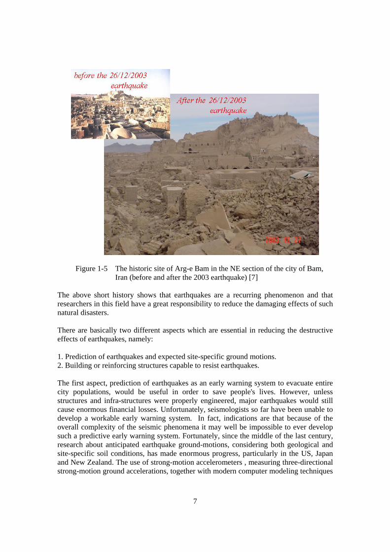
Figure 1-4 Anchorage, Alaska, 1964 [1] The recent disaster in Bam, Iran occurred in December 2003. The earthquake claimed the life of 42,000 people; more than 50,000 persons were injured and about 100,000 people were left homeless. The epicenter was located virtually underneath the city of Bam; a section of the Bam fault, which passes close near the city, was reactivated in the December 2003 earthquake [7].

7

Figure 1-5 The historic site of Arg-e Bam in the NE section of the city of Bam, Iran (before and after the 2003 earthquake) [7]

The above short history shows that earthquakes are a recurring phenomenon and that researchers in this field have a great responsibility to reduce the damaging effects of such natural disasters. There are basically two different aspects which are essential in reducing the destructive effects of earthquakes, namely: 1. Prediction of earthquakes and expected site-specific ground motions. 2. Building or reinforcing structures capable to resist earthquakes. The first aspect, prediction of earthquakes as an early warning system to evacuate entire city populations, would be useful in order to save people's lives. However, unless structures and infra-structures were properly engineered, major earthquakes would still cause enormous financial losses. Unfortunately, seismologists so far have been unable to develop a workable early warning system. In fact, indications are that because of the overall complexity of the seismic phenomena it may well be impossible to ever develop such a predictive early warning system. Fortunately, since the middle of the last century, research about anticipated earthquake ground-motions, considering both geological and site-specific soil conditions, has made enormous progress, particularly in the US, Japan and New Zealand. The use of strong-motion accelerometers , measuring three-directional strong-motion ground accelerations, together with modern computer modeling techniques

8

and analyses of site-specific deep-layered soil deposits under seismic excitation have provided engineering seismologists with invaluable tools, for predicting the anticipated site-specific seismic accelerations and developing seismic design spectra necessary for predicting the structural response of buildings and other structures to earthquakes. The second aspect has been the scope of most earthquake engineering research world-wide. Based on extensive research and reliable construction practices, major efforts have been devoted to developing resistant structural building systems in steel, reinforced concrete and timber. Also in this case research efforts have been devoted to both full-scale experimental studies and numerical, computer supported, analyses of the structural response under seismic excitation, in order to develop reliable design rules which have been incorporated in modern seismic design codes. Other than in case of engineered, reinforced concrete-block masonry, seismic research on brick masonry has long been missing because the basically brittle characteristics of masonry made it an unsuitable building material even in regions with small and moderate seismic activities. Only lately, with the potential exposure of masonry in older structures and its use in larger earthquake prone regions, masonry research under seismic conditions has become a subject study. The objective of this research has been focused on evaluating the effectiveness of simple reinforcing methods to improve their seismic resistance. The scope of the research here presented is to develop a cost-effective structural solution for improving the earthquake resistance of, up to three storey high, residential masonry-brick buildings using common German perforated bricks. The experimental studies covered herein describe the design and study of almost full-scale two-storey brick-masonry specimens under earthquake simulated shaking table motions. In the later sections the research target and the results will be discussed in detail.

Figure 1-6 Homeless people are looking at their collapsed building after a destructive earthquake

9

1.2 Seismological Aspects Although it is beyond the scope of this work to discuss in detail the basics of seismology, a brief review shall provide a basis for assessing seismic risk and for estimating structural response.

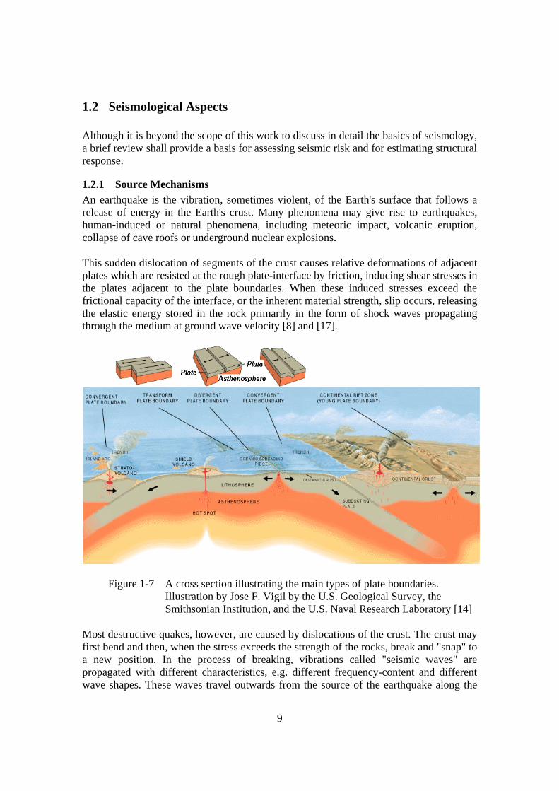
1.2.1 Source Mechanisms An earthquake is the vibration, sometimes violent, of the Earth's surface that follows a release of energy in the Earth's crust. Many phenomena may give rise to earthquakes, human-induced or natural phenomena, including meteoric impact, volcanic eruption, collapse of cave roofs or underground nuclear explosions. This sudden dislocation of segments of the crust causes relative deformations of adjacent plates which are resisted at the rough plate-interface by friction, inducing shear stresses in the plates adjacent to the plate boundaries. When these induced stresses exceed the frictional capacity of the interface, or the inherent material strength, slip occurs, releasing the elastic energy stored in the rock primarily in the form of shock waves propagating through the medium at ground wave velocity [8] and [17].

Figure 1-7 A cross section illustrating the main types of plate boundaries. Illustration by Jose F. Vigil by the U.S. Geological Survey, the Smithsonian Institution, and the U.S. Naval Research Laboratory [14]

Most destructive quakes, however, are caused by dislocations of the crust. The crust may first bend and then, when the stress exceeds the strength of the rocks, break and "snap" to a new position. In the process of breaking, vibrations called "seismic waves" are propagated with different characteristics, e.g. different frequency-content and different wave shapes. These waves travel outwards from the source of the earthquake along the

10

surface and through the Earth at varying speeds depending on the material through which they move. Some of the vibrations are to be audible by man, while others are of very low frequency and maybe recorded by instruments or are audible for some animals. These vibrations cause the entire planet to quiver or ring like a bell or tuning fork; this it the reason that waves can be recorded around world.

1.2.2 Seismic Waves The rupture point within the Earth's crust represents the source of the energy emission. It is variously known as the hypocenter, focus, or source. For a small earthquake, it could be reasonable to consider the hypocenter as a point source, but for very large earthquakes, where rupture may occur over hundreds or even thousands of square kilometers of fault surface, a point surface does not adequately represent the rupture zone. In such cases the hypocenter is generally considered as the point where rupture is first initiated; the rupture requires a finite time to propagate over the entire fracture surface.

Figure 1-8 Deformed railroad track after strong earthquake Whatever the case of the earthquakes may be, they generate two types of waves: P and S waves. Because of the difference in velocity of propagation of these waves one would expect accelorograms at some distance away from the focus to consist of two separate trains of oscillation, one for each type of the waves. But analysis of the recorded data from such accelerograms is very complicated, and the train of S-waves always begins before that of P- waves has subsided.

11

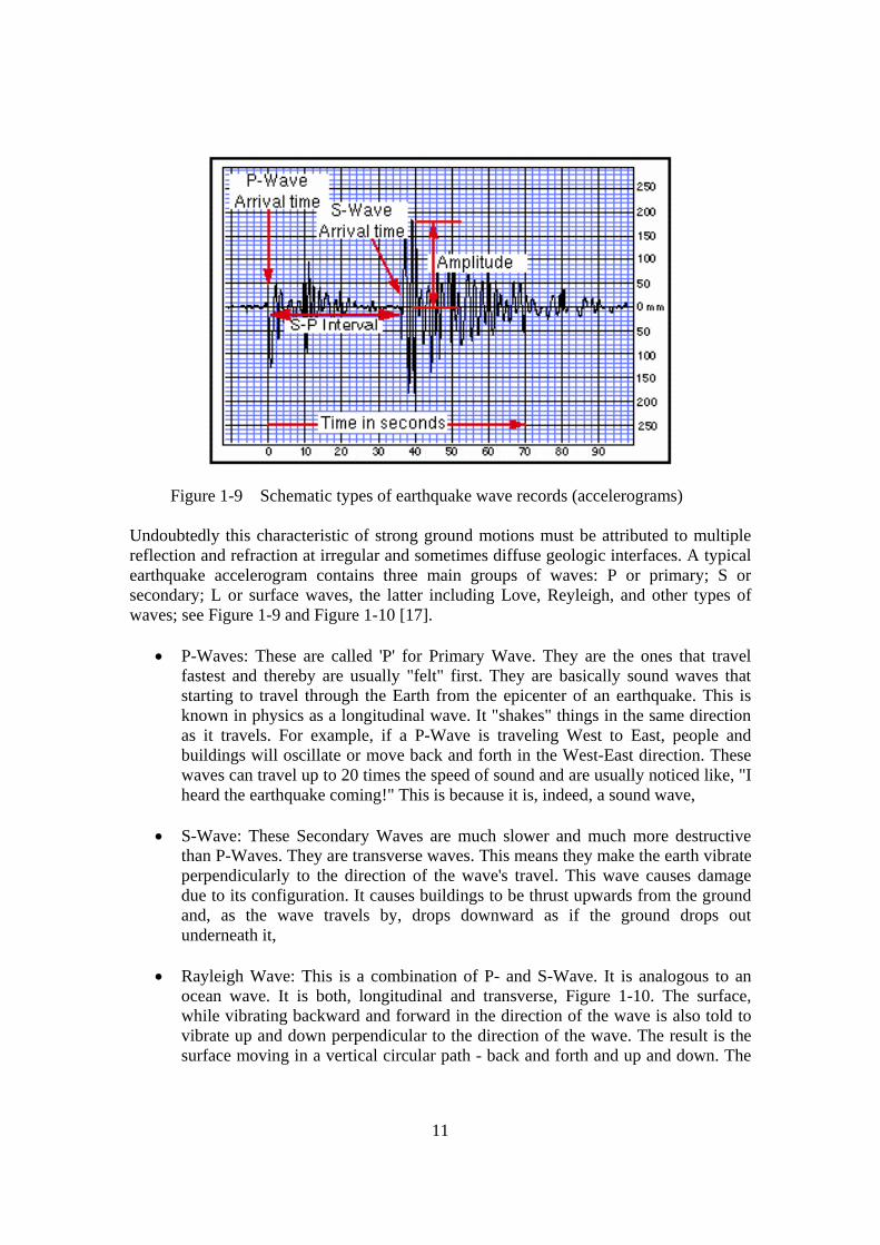
Figure 1-9 Schematic types of earthquake wave records (accelerograms) Undoubtedly this characteristic of strong ground motions must be attributed to multiple reflection and refraction at irregular and sometimes diffuse geologic interfaces. A typical earthquake accelerogram contains three main groups of waves: P or primary; S or secondary; L or surface waves, the latter including Love, Reyleigh, and other types of waves; see Figure 1-9 and Figure 1-10 [17].

• P-Waves: These are called 'P' for Primary Wave. They are the ones that travel fastest and thereby are usually "felt" first. They are basically sound waves that starting to travel through the Earth from the epicenter of an earthquake. This is known in physics as a longitudinal wave. It "shakes" things in the same direction as it travels. For example, if a P-Wave is traveling West to East, people and buildings will oscillate or move back and forth in the West-East direction. These waves can travel up to 20 times the speed of sound and are usually noticed like, "I heard the earthquake coming!" This is because it is, indeed, a sound wave,

• S-Wave: These Secondary Waves are much slower and much more destructive

than P-Waves. They are transverse waves. This means they make the earth vibrate perpendicularly to the direction of the wave's travel. This wave causes damage due to its configuration. It causes buildings to be thrust upwards from the ground and, as the wave travels by, drops downward as if the ground drops out underneath it,

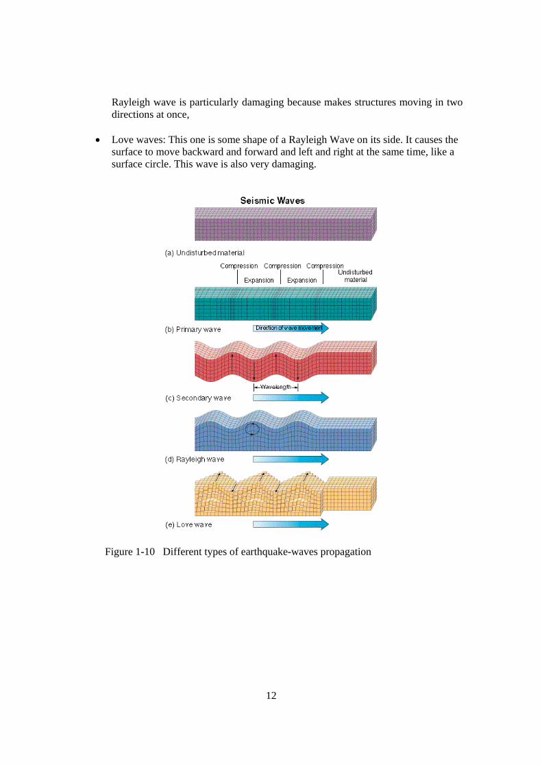
• Rayleigh Wave: This is a combination of P- and S-Wave. It is analogous to an

ocean wave. It is both, longitudinal and transverse, Figure 1-10. The surface, while vibrating backward and forward in the direction of the wave is also told to vibrate up and down perpendicular to the direction of the wave. The result is the surface moving in a vertical circular path - back and forth and up and down. The

12

Rayleigh wave is particularly damaging because makes structures moving in two directions at once,

• Love waves: This one is some shape of a Rayleigh Wave on its side. It causes the

surface to move backward and forward and left and right at the same time, like a surface circle. This wave is also very damaging.

Figure 1-10 Different types of earthquake-waves propagation

13

1.3 Masonry Structures through Time Masonry is the oldest, most tested and trusted building material ever used. As new systems come into the construction market, designers return to improve the strength of masonry.

Figure 1-11 Brick making in Egypt, as depicted on the tomb of Rekmyre

(Rekhmyra) of the 18th dynasty (1500 B.C.) Masonry systems have many advantages over other competitive systems such as concrete, precast, and steel under compression forces. It has the following benefits:

• Design flexibility with colors, textures shapes, • Materials that allow designers to build a project that can blend into and highlight

the strengths of the community, • Durability, • Low maintenance, • Acoustics, • Energy saving, • Fire resistance, • Mold resistance, • Speed of construction, etc.

14

Architecturally, masonry is a highly flexible system which allows for a maximum level of design options. Over times, according to the available methods and materials, designers preferred using masonry because they know that its flexibility in use allows them to design structures as envisioned by the rulers of those times in the past and by the nowadays-clients. For example concrete masonry units, brick, stone, glass block and tile offer hundreds of design options which no other system can deliver. A masonry system is a user defined method of incorporating varied masonry materials into a structure. No other construction method can offer the full range of features that a masonry system can deliver [16]. The history of masonry is very old. For example the Egyptian Pyramids, the Coliseum in Rome, the Great Wall of China, India's Taj Mahal - some of the world's most significant architectural achievements have been built with masonry. The first masonry material to be used was probably stone. In the ancient Near East, the evolution of housing was from huts, to apsidal houses, and finally to rectangular houses. The earliest example of the first permanent stone masonry houses can be found near Lake Hullen, Israel (9000-8000 BC), where dry-stone huts, circular and semi-subterranean, from 3 m to 9 m in diameter have been found. At Kangawar near Kermanshah, Iran remains of a large structure with masonry of 'huge square stones' above which was a colonnade, assigned by Herzfeld to the Seleucid period on the basis of presumed differences from Parthian building methods; these, however, are not known from any indubitable Parthian building of Iran. From the temple which Antiochus III ordered to be built in Nihavend for the cult of his wife Laodicea, nothing remains. Presumably Seleucid structures followed Greek tradition in the use of good stone, well-dressed masonry, and marble or limestone columns, all of which were surely plundered by the local peasantry, who are avid for worked stone in most parts of the Near East [22]. Through civilization, architects and builders have chosen masonry for its beauty, versatility, durability; some of these structures were built up because of empire's desires or for honor of a country. Masonry is resistant enough to fire, earthquakes (in case of good design), and sound. The level of complexity involved in masonry work varies from laying a simple masonry wall to installing an ornate exterior or high-rise building. Whether he is working with brick, block, tile or stone, and regardless of the level of craftsmanship involved, the skill and precision of the mason can probably never be replaced by machines.

15

Figure 1-12 Coliseum in Rome The most frequently used products, are clay brick and concrete block. Clay brick has been in use for at least 10,000 years but possibly for as long as 12,000 years [12]. Brick is man's oldest manufactured product. Sun-baked clay bricks were used in the construction of buildings more than 6,000 years ago. The technique of dry stone block was greatly improved and remarkable structures were built using this technique, as the Coliseum, (1st century A.D.) and Segovia's aqueduct (1st century A.D.) [21]. Sun-dried bricks were widely used in Babylon, Egypt, Spain, South America, the Indian lands of the United States, and elsewhere. Wide usage is illustrated by the word "adobe", which is now incorporated in the English language but is a Spanish word based on the Arabic word "atob", meaning sun-dried brick. In order to prevent distortion and cracking of the clay shapes, chopped straw and grass were added to the clay mixture. The next big step in enhancing brick production occurred about 4000 B.C. At that time manufacturers began producing brick in uniform shapes. Along with the shaping of brick, the move from sun baking to firing was another important change. The practice of burning bricks probably started with the observation that the brick near a cooking fire or the brick remaining after a thatch roof burnt seemed to be stronger and more durable. To make burnt brick, an adequate supply of fuel was necessary, which may have partially accounted for the continued use of sun dried bricks in the Near East. A very early example of burnt brick mass production is given by an up draught kiln excavated in Khafaje, Iraq, dating from the third millennium BC [20]. Through the centuries the methods for producing bricks have continued to evolve. Today, the standard brick size of the bricks varies according to its duty and requirements. Brick is composed of shale and clay and is fired in kilns of approximately 900 degrees Celsius. The firing process causes the clay particles to bond chemically. As brick construction became more elaborate, the use of bricks became more sophisticated. The evolution of brick construction design led, in part, to the development of concrete blocks. The manufacturing and uses of concrete blocks evolved over a long period of time. This evolution was prompted by the development of cavity walls. When originally developed, cavity walls consisted of two separate brick or stone walls with about a 5 cm air space between them.

16

Figure 1-13 India's Taj Mahal Cavity walls were developed to reduce the problems associated with water penetration. Water that would seep inside the outer wall would then run down that wall, while the inside wall would remain dry. Cavity walls soon became recognized as the best way to build, not only because they helped reduce problems with water penetration, but because they could support a heavy load such as a roof or floor. In 1850 a special block with air cells was developed. Over the years modifications to this product were introduced until the industry arrived at the standardized product we see today.

Figure 1-14 The Great Wall of China Concrete blocks are produced with a mixture of cement, sand, and crushed stone, or lightweight aggregate. Today's concrete block plants are totally automated. The raw materials are loaded from trucks or railroad cars into bins. From there the mix is weighed, transported to a mixer, and fed into the block machine. If necessary, color is added. It takes the machine about six seconds to mold a block. The freshly molded blocks are put into pallets and placed in steam-curing rooms. After the curing process, they are stacked and taken to a storage yard for delivery. Some of the recent developments, e. g. a low dimensional variation of the units combined with improved building tools or large

17

calcium-silicate units combined with modern stacking techniques resorting to machinery, have led to increased labor productivity and reduced costs. In North America, masonry is used nowadays primarily as a cladding system or infill non-load bearing walls, in Germany masonry is primarily used in load bearing systems. After more than 6000 years, masonry is still used today.

1.4 Masonry Structure in Earthquake Engineering Masonry structures are considered problematic in earthquake engineering, for example the complications of any kind of masonry structure under cyclic loads and the lack of clear strategy for modeling masonry systems. Because of the broader use of steel and reinforced concrete in modern earthquake resistant construction, researchers have spent most of their attention to these structural systems. Hence, this section covers only a short discussion on the philosophy of earthquake engineering and the behavior of masonry structures in previous earthquakes.

1.4.1 Earthquake Engineering Philosophy Every year earthquakes kill any people around the world and cause huge financial losses. Earthquake engineering can be defined as the branch of structural engineering devoted to minimizing earthquake hazards. In this broad sense, earthquake engineering covers the investigation, solution and practical application of solving the problems created by damaging earthquakes, more specifically in planning, designing, constructing and managing earthquake-resistant structures and facilities. The philosophy of earthquake design for structures other than essential facilities has been well established and is proposed as follows:

• To avoid collapse or serious damage in rare major ground shaking in order to protect human life,

• To prevent structural damage and to minimize non-structural damage in occasional moderate ground shaking,

• To prevent non-structural damage in frequent minor ground shaking. This philosophy is in complete accordance with the concept of comprehensive design. The comprehensive design approach specifies the damages to the structures may result of different seismic effects. These effects can be classified as direct and indirect. Direct effects can be divided into two main groups:

1. Ground failures (or instabilities due to ground failures) for example: • Surface faulting or fault rupture, • Vibration of soil (or effects of seismic waves), • Ground cracking, • Liquefaction, • Differential settlement, • Lateral spreading,

18

• Landslides.

2. Vibrations transmitted from the ground to the structure. And indirect effects like:

• Tsunamis, • Landslides, • Floods, • Fires.

However, current design methodologies in masonry construction fall short of realizing the objectives of this general design philosophy. Considering however the importance of masonry structures in the field of civil engineering, there is a strong need to develop safe design criteria in consideration of the potential earthquake effects on the masonry structures. Hence the need for research in developing earthquake-resistant design requirements for masonry structures leads researchers to pursue both experimental and analytical investigations.

1.4.2 Masonry Behavior in Previous Earthquakes It is impossible to design seismic resistant structures efficiently without understanding the ways in which they are damaged by earthquakes. The design process is not simply a matter of analysis, calculation and following codes. A practical knowledge of the building behavior in earthquakes is essential, especially for masonry with its highly complex behavior under dynamic loads. Recent research appropriately focuses on defining the behavior of masonry under cyclic loads; however, most codes try to improve the masonry behavior by strengthening the material with steel or glass-fiber material. In past earthquakes most destructive failures were related to ancient material. Based on earthquake-damage studies the principal forms of damage can be described, and are presented in Section 2.2, together with some explanation of the mechanics of failure. The behavior of masonry structures in previous earthquakes has shown that these structures are far more susceptible to damages and failure than other type of structures, built of reinforced concrete or steel. Failure of unreinforced masonry is so common that it is not being used in earthquake resistant construction almost forgotten. In fact, many earthquake codes ban the use of unreinforced masonry in load bearing structural systems. However, considering the ease of construction, economic reasons still make it a very widely used system, both for low-rise structural walls ( in 3-storeys buildings) or as an infill material in framed structures. In-plane failures of both reinforced and unreinforced masonry are common. Masonry is very stiff and brittle in-plane so that the forces transmitted by ground shaking are high and failure is accompanied by a marked reduction in strength and stiffness. Damage normally comprises either collapse or diagonal cracking in both directions ("X" cracking). Cracks, which will often be located between adjacent openings, will frequently

19

follow the mortar joints (also the crack pattern differs in stiffness and strength of the units or used mortar), Figure 1-15.

Figure 1-15 Typical "X" cracking of masonry in this Anchorage, Alaska School illustrates the effect of reversing horizontal shear forces during the earthquake. Shear stresses are concentrated opposite the window openings

1.5 The Seismic Activity of Germany Germany is situated geologically inside the Eurasian plate, far from active plate boundaries, which might cause strong earthquakes. Nevertheless, the seismicity in parts of Germany is remarkable and could be damaging, too. Our knowledge about historical earthquakes is, like everywhere, strongly bounded to the social and cultural development. It is obvious that it needed people, who were familiar with the art of writing - mostly monks in early times - to make a note of sudden and damaging earth shaking to hand down the existence of such events. The documents had to outlast the centuries of evils like fire and war. It also needed people who had an interest in keeping these records for the future. It is noticeable to know that these storeys or reports are sometimes exaggerated, because they always reflected the human-sense of the writer [5]. Hence, history has not delivered an acceptable document for usage in any earthquake design approach of later structures. The first computerized earthquake catalogue of the Federal Republic of Germany and adjacent areas was issued by BGR (Bundesanstalt für Geowissenschaften und Rohstoffe in Hanover) in 1978. Since then the catalogue has been continuously improved and supplemented and covers now the period from AD 800 to 2003. This earthquake

20

catalogue starts with the year 800 AD, the year of the coronation of the emperor Charlemagne and the beginning of a new epoch in government and culture. Over the following centuries, the documents about earthquakes grew in number and variety. During the Middle-Ages, earthquakes as well as plague and cholera were one of the most destructive disasters which threatened human life. Within the Age of Enlightenment, natural sciences developed and natural phenomena themselves as well as their history were studied. The publication of the first newspapers in the 18th century brought an important progress in written documents describing local events. But as it is today, reports must be taken critically, because exaggerations or incorrect statements are not uncommon [6]. The other view that makes theses types of documents unreliable is the lack of specified criteria for evaluating and describing earthquake damages that are now commonly used in codes (e.g. Mercalli scale). The installation of the first seismographs at the beginning of 20th century marks the transition from the qualitative description of an earthquake to a quantitative measure. Since the sixties, many local seismometer stations have become operational. Now, seismologists are able to monitor and locate even very small events or vibrations anywhere around the World. Beside the instrumental registration of earthquakes events, the continuation observation of macroseismic events remain indisputable the basis for scientific research in the World's seismicity and plate tectonics. In 1954, the Earth was divided into 50 seismic regions. In 1965 these regions were further subdivided into a total of 728 regions. The boundaries were drawn along latitudes and longitudes in order to assign automatically an epicenter to a named region. The result was a very rough subdivision providing little specific information. For example, region 543, was named "Germany" and extended from eastern France to eastern Poland. The distribution of earthquakes in Germany in space and time is far from uniform as seen in Figure 1-16. The wide areas of Northern Germany, the German lowlands, are nearly free of earthquakes. The few known events reached a maximum intensity of VI - MSK. Also in the central part of Germany, earthquakes are very rare. The main activity is concentrated in the western parts and in the east. Over the centuries, a steady seismicity is documented for the northwestern border of the Alps, the Lake of Constance, the Upper Rhine Graben between Basel (Bale) and Frankfurt/Main (Frankfort) and for the Lower Rhine Area northwest of Bonn. Very active in the 20th century is the Swabian Jura south of Stuttgart. In Eastern Germany, the regions around Leipzig and Gera and the Vogtland area, east of Hof, show a remarkable activity. In all areas the maximum intensity never exceeded intensity VIII, the maximum measured local magnitude ML was 5.9 (13 April 1992, Roermond/NL, Lower Rhine Area, intensity VII MSK). Unusual earthquake activities during the last century have been registred in the Swabian Jura south of Stuttgart (although historically a region with low seismicity; the recent earthquakes have been the most important in Central Europe north of the Alps).

21

Figure 1-16 Earthquake damaging in Germany between 800 and 1998 In Central and Western Europe, the new earthquake zones in connection with the corresponding design ground acceleration values will lead in many cases to earthquake actions which are remarkable higher than defined by the design codes used up to now in Central Europe. Hence, in the new codes the more realistic values of earthquakes load for design and analyzing the structures have to be considered.

22

1.6 German Earthquake-Code (DIN 4149) In the last few decades, a considerable amount of experimental and analytical research on the seismic behavior of masonry walls and buildings has been carried out, although it has been discussed in comparison with other types of civil engineering structures these activities were not sufficient. The investigations resulted in the development of methods for seismic analysis and design, as well as new technologies and construction systems. After many centuries of traditional use and decades of allowable stress design, clear concepts for limit state verification of masonry buildings under earthquake loading have recently been introduced in codes of practice. Unreinforced masonry is used for most of housing buildings in Germany, Belgium, the Netherlands, and Austria. For reinforced concrete structures, steel and timber, the new seismic code regulations can be implemented with less problems than for masonry structures, since unreinforced masonry cannot make use of a large reduction of accelerations resulting from ductile earthquake response. Unreinforced masonry in many cases does not show significant ductility, especially when perforated bricks are used with regard to thermal insulation as desirable in these countries. In current drafts of ENV 1998-1, a rather low ductility/behavior factor of q=1.5 is recommended for unreinforced masonry to reduce the design response accelerations in comparison to the linear elastic response values. The implementation of the new codes will lead to the situation, that a huge amount of buildings, executed in masonry construction and designed according to the old codes, cannot be proved to be earthquake resistant according to the new generation of codes. Furthermore, it may become difficult or even impossible to design and execute masonry buildings in a similar way as until now (unreinforced masonry). For low seismicity areas, on the other hand, the use of reinforced or confined masonry is problematic with respect to economical aspects. Nevertheless this investigation’s target is to find new methods for designing and keeping safe masonry structures by attention to the local seismicity in the countries mentioned above. The design procedure for masonry structures in DIN 4149 in order to determine earthquake forces is like other codes that in brief explanation are:

1. Specify the horizontal load as an earthquake load for both main directions of the structure according to the German Earthquake Code (DIN 4149 is source code for calculating earthquake load and design of building). This step includes:

• Calculating of ground acceleration, • Select related response spectrum by attention to the

geographical position of the structure in the country, soil specification of the area, fundamental-period of the structure and geometry of the structure,

• Use the suggested method of the code for distributing the earthquake load on the structure,

23

• Calculate total vertical mass of the structure by using the appropriate loading factor and specified safety factor, this mass includes masses of the walls, slabs, roofs, live loads, etc,

2. Specify the weak direction of the structure for imply the earthquake load

on the structure, and find out the bearing walls in that direction, 3. Calculate geometry and mechanical properties of the selected walls in

weak direction, 4. Calculate the vertical load of each different wall by attention to its loading

span and geometry, 5. Calculate the share of the horizontal load on every single wall that is

specified in step 3, 6. Overturning moment and eccentricity calculation for the wall and

specification of all walls´ stability.

In following other useful strategies (other criteria for understanding the behavior of the structures under the cyclic load) are stated for example:

7. Capacity of the walls has to be included to all calculations specify the

maximum ability of every wall under loading and the difference between the demanded load and the capacity of the structures,

8. Specify capacity curves of the structures in order to find out the resistance of the structure against the earthquake load.

24

1.6.1 Seismic Zoning Map The seismic map of Germany in DIN 4149 is classified into two different categories. First, the seismic zoning map and second the map of the geological subsoil classes. Figure 1-17 shows the seismic zoning map of Germany, reference DIN 4149. The figure shows four different areas according to their risk ability. These four areas divided from Zone 0 to Zone 4 with increasing risk of seismic hazard. As it is shown in this figure the areas with higher risk are in the west and southwest of Germany. Figure 1-18 shows the subsoil division. There are three different subsoil classes, Table 1-1:

Table 1-1 Description of subsoil classes according to DIN 4149 [52]

Subsoil Class

Description

A rock, hard soil SV > 800 m / s, missing or very thin soft sediments

B

shallow sedimentary basins and transitions zones, < 100 m soft sediments, above hard rocks or tertiary sediments up to 500 m thickness, SV increasing up to 1,800 m / s, at the transition to Mesozoic rocks, sudden increase of SV up to 2,000-2,500 m / s, at the transition to hard rock, sudden increase in SV of values larger 3,000 m / s

C

deep sedimentary basins > 100 m soft sediments, underneath hard soil with SV > 800 m / s or tertiary sediments > 500 m with increasing SV up to 1800

m / s

25

Figure 1-17 Seismic zoning map of Germany, DIN 4149

26

Figure 1-18 Map of the geological subsoil classes of Germany

27

Geological subsoil classes and seismic zoning map of Germany are shown together in Figure 1-19.

Figure 1-19 Map of the subsoil classes and seismic zoning map of Germany

28

Figure 1-20 shows seismic hazard map of Germany, Austria and Switzerland with added epicenters of tectonic earthquakes. The figure shows earthquake hazard in term if intensities values for a non-accidence probability of 90% within 50 years, [40], [41], [42], [43].

Figure 1-20 Seismic hazard map of Germany, Austria and Switzerland

29

1.7 Research Goals In the past masonry structures were erected by the time-honored method of trial and error. The traditional methods and rules-of-thumb were passed, sometimes in secrecy, from one generation to the other. With mathematical availabilities and today’s technology, it is possible to predict and analyze most of the projects not only in the field but also in the laboratory. The main idea of this research is to generate a new economic method for keeping more safe masonry structures during earthquakes in low risk seismic regions, particularly in Germany and countries in Central Europe. A capacity design approach, based on the Corner-Gap-Element, shall be verified experimentally as well as by numerical simulations. Finally, engineering models for the necessary design checks shall be developed. Shaking table tests in the earthquake engineering laboratory of NTUA (National Technical University of Athens) have been performed in order to confirm the capacity design concept enabled by Corner-Gap-Element. Impact effects due to sudden crack closing have been considered as a conceivable objection against the use of Gap-Elements shall be studied. Other than static cyclic or pseudo-dynamic tests, shaking table tests can simulate all dynamic effects which can occur during an earthquake. So shaking-table tests had to be preferred in order to investigate the behavior of such masonry walls. The tests shall enable a comparison of the seismic behavior between walls being designed with and without Gap-Elements. Since the masonry shall be protected from severe stresses, the behavior of masonry with unfilled perpend joints, i. e. with no mortar in the vertical joints, is expected to be also satisfactory. The tests shall enable a proof of this hypothesis too. Finally this research shall address the following aspects:

• To provide appropriate earthquake resistance for masonry structures during minor and major earthquakes for the different zones,

• To adopt solution techniques and to develop new models which are stable and economical in the entire loading regime of the structure,

• To develop a constitutive and useable model for unreinforced masonry which includes softening and incorporates all failure mechanisms such as tensile, shear and compressive failure,

• To discuss the new outlook and its ability to prevent structural damage and to minimize non-structural damage in bearing masonry walls,

• To avoid collapse or serious damage in rare major ground shaking for masonry structures,

• To verify the developed models by comparing the predicted behavior with the behavior observed in experiments on different types of structures,

30

• To develop a method which is able to predict the failure mode and ultimate load with reasonable agreement with experimental values,

• Demonstration of the applicability of the models in engineering practice with potential in marketing by attention to establish a teachable method for bricklayers.

31

2 STATE OF KNOWLEDGE

2.1 Introduction “Main purpose of the research is to create a base for general approach to structural masonry. This includes closing the gap between theory, mechanicals models and material testing on the one hand, and the structural practice on the other hand, which should result in clearer insight and scientific basis for the behavior of masonry structures”, the CUR PAC4 committee[15]. Cheap materials and simple construction in comparison with other structures such as steel or concrete models and enough knowledge about the way of building are important views for constructing masonry structures. Masonry structures have a good position in normal buildings with less than two storeys. The reason is related to the history of civilization and using of different types of masonry material. As an example after invention of concrete, masonry structures had their interest in most of the countries. Masonry structures are discontinua at the engineering scale. They consist essentially of intact blocks (such as stones or clay) separated by discontinuities (interfaces, bed joints, cracks). These discontinuities have a strong non-linear effect and dominate the strength and deformation behavior of masonry structures. In general, continuum models are inadequate in predicting the response of such systems to loading and unloading, but the numerical models (discussed in next chapter) based on the Distinct Element Method (DEM) seem to be more appealing for dealing with these problems. The evolution of the old techniques into the new and modern applications occurred unsuccessfully. Presently, prejudices against structural masonry persist, based on the claim that it is expensive, fragile, and unable to withstand earthquakes and dependent on unreliable workmanship and unknown quality. As a consequence, only few resources have been put in structural masonry research, the current codes of practice are underdeveloped and there is a lack of knowledge about the behavior of this composite material. The fundamental point of today’s research in structural masonry is to rationalize the engineering design of structural masonry. Considerable research effort has been made in the last two decades but progress has been hindered by the lack of communication between analysis and experimental investigations that this project tried to achieve for closing this gap. Masonry has to be regarded as a multi-component material being constituted of masonry units and mortar. The interface between mortar and units may be regarded as a third component, which in many cases governs the behavior of masonry walls. A wide variety of materials is available to produce masonry units, e. g. clay, calcium-silicate, lightweight concrete, and autoclaved aerated concrete, different kinds of mortar may also be used. In the last decades, lightweight mortar with good thermal insulation properties as well as

32

thin-layer mortar became more and more important for masonry in housing constructions and begin to replace partially traditional mortars based on limestone and/or cement. Due to this large variety in basic materials, masonry can hardly be treated by a small set of simple design formulas. It is essential to know the relevant material parameters from all basic constituents as well as bond characteristics in order to come up with realistic models for the mechanical behavior. A considerable amount of research has been done with respect to design models and numerical modeling of masonry. This has been attempted by discrete modeling of units and mortar layers as well as by smeared models; however, theoretical modeling alone cannot replace experimental investigations, especially in the case of earthquake loading, where alternating loading occurs. Experimental investigations still have to be considered to be inevitable in order to assess especially:

• The post peak behavior and ductility of masonry structures, • The degradation of strength and stiffness with increasing number of load cycles.

Several experimental investigations have been devoted to gain a better understanding of the structural behavior of masonry structures subject to earthquake excitation. In addition, different methods to strengthen masonry walls have been investigated, such as:

• Reinforcing masonry by steel elements (wires / re-bars ), • Reinforcement by non metallic reinforcement elements (fiber composites), • Confining masonry by R/C elements.

The current draft of the European seismic design code prEN 1998-1 already considers these developments in the chapter on masonry structures. In contrast to all other chapters related to building materials, nothing is said there about capacity-design as a method to ensure ductile structural behavior. This reflects the current state of technology where masonry in many cases is regarded as a mainly brittle material. Reinforcement of masonry can improve both, ultimate load capacity as well as ductility. Reinforcement has been stated by the masonry industry to be an important goal with respect to marketing aspects. It seems to be important to avoid a type of masonry construction which is similar to reinforced concrete because otherwise not only slabs and columns would be made of reinforced concrete but also walls. It would have a big impact on the market share of masonry in Central Europe. However, it is possible to design masonry structures to behave in a ductile manner, even without reinforcement. This is enabled by the so called Corner-Gap-Element which is supposed to be able to protect critical zones of masonry structures from high stresses. In regions of negligible or low seismicity, structures are normally designed mainly for vertical (gravity) loads. The heavy weight of massive building structures typically can help to avoid or to limit tensile stresses in the load bearing masonry walls due to horizontal loads, such as wind. Many buildings, hence, can be classified as so called Zero

33

Premium Systems, where nothing has to be done in addition to the design for vertical loads in order to be able to withstand also horizontal loads. Tensile stresses, however, are a big problem for masonry. In the case of an earthquake, big (inertia) forces can develop leading to tensile stresses in masonry. This leads to cracking, e. g. in the horizontal mortar joints. Due to the lack of significant tensile load carrying capacity, the capacity of masonry walls against overturning moments is limited. A tool to improve the seismic behavior of masonry walls in that respect will be ‘Corner-Gap-Element`, (see 2.4.3).

2.2 Masonry Structures and Lateral Load Latest researches in the filed of masonry structures are not comparable with the researches of the other types of structures. The reason is related to the complicated behavior of masonry structures compared with other structures. The knowledge of masonry structures in the field of dynamics is still not appropriate for good evaluation and analyzing the masonry material. In Germany, there is a limited amount of research going on in the field of masonry structures with effect of dynamic loads and experimental investigation. In European countries as well as other countries around the world, masonry materials have been selected as a primary material for constructing the buildings. Multi- storeys building have never been possible to construct, because of earthquake hazards. In some special countries in Europe, such as Great Britain, far away from the earthquake belt, there was the chance to construct high masonry structures with many storeys. Nonlinear behavior, non homogeneous material, huge number of cracks on the one hand and plane action of the member of masonry structure on the other hand caused complicate behavior in masonry structures. For overcoming the problem, mostly the Finite Element Method can show the stress distribution or rupture pattern [3]. For explained reasons small size modeling of masonry buildings does not contain the reality of the units and mortar connections, because it is impossible to model units and mortar stiffness. Modern technology made many opportunities for modeling masonry structures with full scale size, for example shaking table, two-way hydraulic jacks with reaction wall or dynamics actuator. The new facilities give a lot of important information about masonry, for instance resistance of material, stiffness of members, failure pattern and recording the responses of the structure with high sensitive accelerometer or LVDT. In low seismicity regions normally masonry structures designed for vertical weight load and horizontal wind load because of heavy weight they can be stable against wind load in most cases. In these regions, walls designed for compressive stress due to weight, flexural stress from load eccentricities on bearing walls and flexural stress from wind load act perpendicular on wall plane. There have been many researches on this subject for calculating the forces in masonry structures and masonry walls under loading. In 1981,

34

the research for calculating these forces on masonry structures was published by Hendry [2]. Masonry buildings are brittle structures and one of the most vulnerable of the entire building stock under strong earthquake loading. Hence, it is very important to improve the seismic behavior of masonry buildings. A number of earthquake-resistant features can be introduced to achieve this objective. Ground vibrations during earthquakes cause inertia forces at locations of mass in the building. These forces travel through the roof and walls to the foundation. The main emphasis is on ensuring that these forces reach the ground without causing major damage or collapse. Figure 2-1 shows the three components of a masonry building (roof, wall and foundation), the walls are most vulnerable to damage caused by horizontal forces due to earthquake.

Figure 2-1 Basic components of masonry building [19] Figure 2-2 shows masonry wall under loading, vertical load affected by dead loads or live loads and horizontal loads which may be generated by wind or earthquake.

Figure 2-2 Masonry wall under vertical and horizontal loading Earthquake loads distribute in the structure according to the walls` position and their actions. For example bearing walls take the loads in both directions, but it does not guarantee to neglect the lateral walls existence. Figure 2-3 shows the interaction of load

35

distribution during the horizontal load. This figure implies two types of actions of the walls in masonry structures: • In-Plane Action, • Out-of-Plane Action. Next section describes the details of walls` action.

Figure 2-3 Schematic lateral load distribution in masonry building [19]

The main parts of every masonry structure that transfers the lateral load to the foundation are the walls with in-plane action. The roof has to be stiff and solid enough to shift its load and anything above it. For example, concrete slabs belong to this category. Figure 2-4 illustrates a masonry building with sub-units detail. Masonry structure includes following parts:

• Roof, • Wall, • Pier, • Spandrel, • Sill, • Foundation.

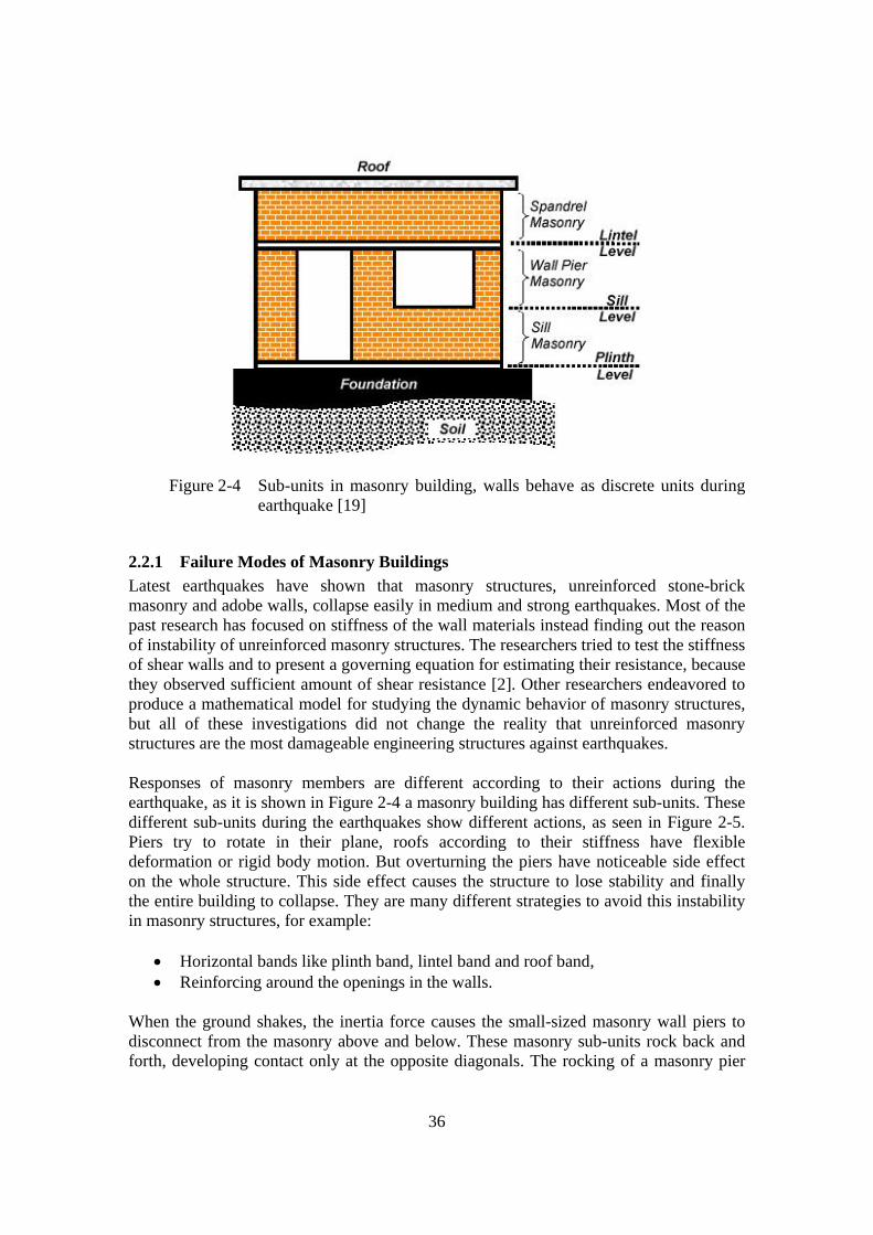
36

Figure 2-4 Sub-units in masonry building, walls behave as discrete units during earthquake [19]

2.2.1 Failure Modes of Masonry Buildings Latest earthquakes have shown that masonry structures, unreinforced stone-brick masonry and adobe walls, collapse easily in medium and strong earthquakes. Most of the past research has focused on stiffness of the wall materials instead finding out the reason of instability of unreinforced masonry structures. The researchers tried to test the stiffness of shear walls and to present a governing equation for estimating their resistance, because they observed sufficient amount of shear resistance [2]. Other researchers endeavored to produce a mathematical model for studying the dynamic behavior of masonry structures, but all of these investigations did not change the reality that unreinforced masonry structures are the most damageable engineering structures against earthquakes. Responses of masonry members are different according to their actions during the earthquake, as it is shown in Figure 2-4 a masonry building has different sub-units. These different sub-units during the earthquakes show different actions, as seen in Figure 2-5. Piers try to rotate in their plane, roofs according to their stiffness have flexible deformation or rigid body motion. But overturning the piers have noticeable side effect on the whole structure. This side effect causes the structure to lose stability and finally the entire building to collapse. They are many different strategies to avoid this instability in masonry structures, for example:

• Horizontal bands like plinth band, lintel band and roof band, • Reinforcing around the openings in the walls.

When the ground shakes, the inertia force causes the small-sized masonry wall piers to disconnect from the masonry above and below. These masonry sub-units rock back and forth, developing contact only at the opposite diagonals. The rocking of a masonry pier

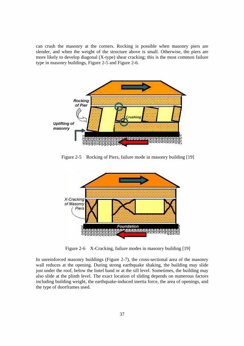
37

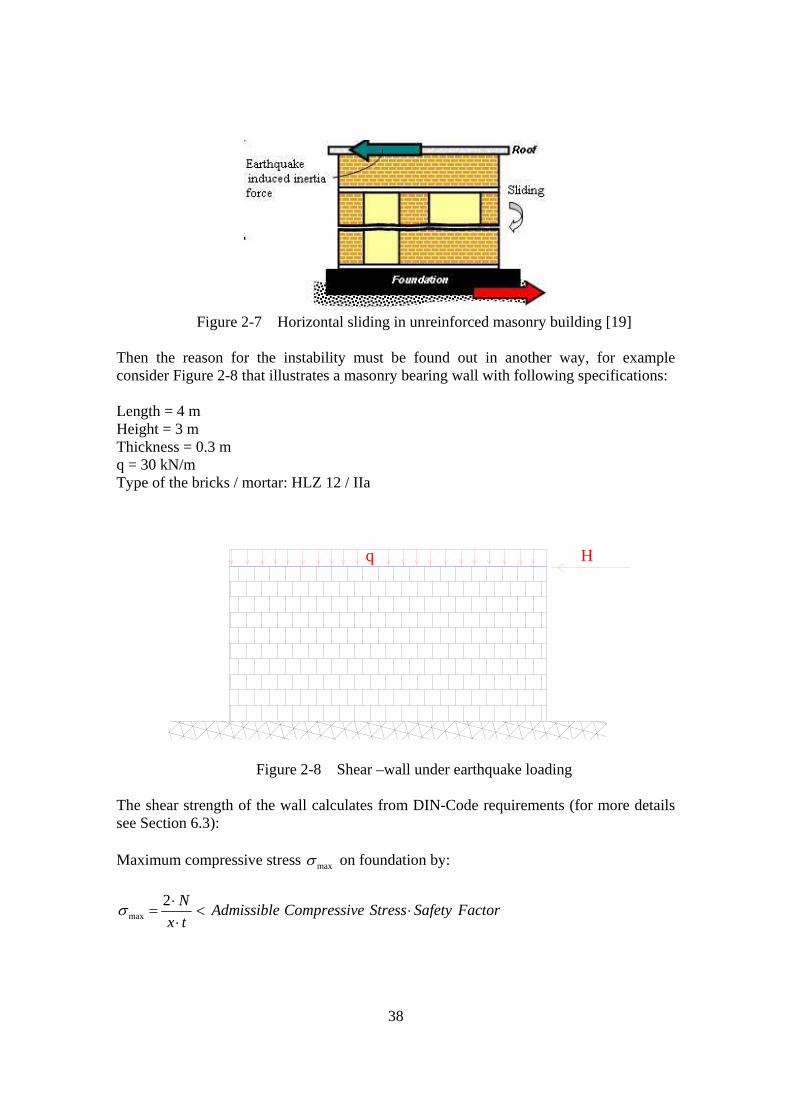
can crush the masonry at the corners. Rocking is possible when masonry piers are slender, and when the weight of the structure above is small. Otherwise, the piers are more likely to develop diagonal (X-type) shear cracking; this is the most common failure type in masonry buildings, Figure 2-5 and Figure 2-6.

Figure 2-5 Rocking of Piers, failure mode in masonry building [19]

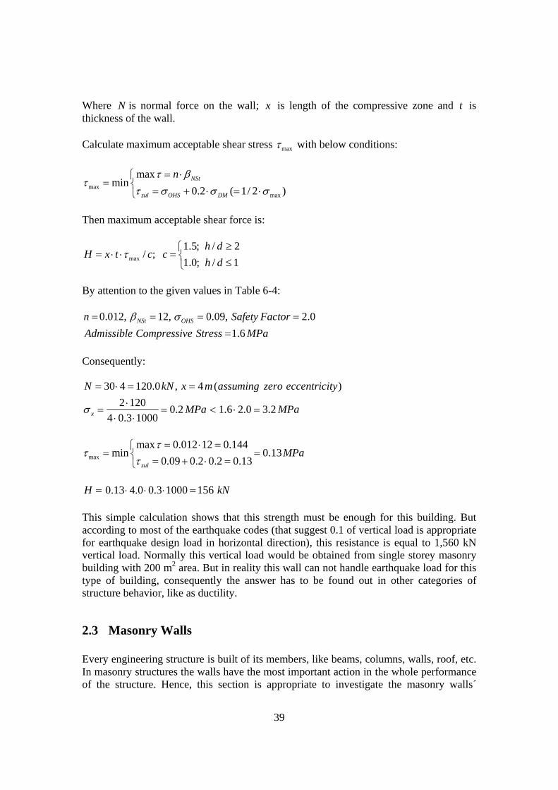
Figure 2-6 X-Cracking, failure modes in masonry building [19] In unreinforced masonry buildings (Figure 2-7), the cross-sectional area of the masonry wall reduces at the opening. During strong earthquake shaking, the building may slide just under the roof, below the lintel band or at the sill level. Sometimes, the building may also slide at the plinth level. The exact location of sliding depends on numerous factors including building weight, the earthquake-induced inertia force, the area of openings, and the type of doorframes used.

38

Figure 2-7 Horizontal sliding in unreinforced masonry building [19]

Then the reason for the instability must be found out in another way, for example consider Figure 2-8 that illustrates a masonry bearing wall with following specifications: Length = 4 m Height = 3 m Thickness = 0.3 m q = 30 kN/m Type of the bricks / mortar: HLZ 12 / IIa

Hq

Figure 2-8 Shear –wall under earthquake loading The shear strength of the wall calculates from DIN-Code requirements (for more details see Section 6.3): Maximum compressive stress maxσ on foundation by:

max2 N Admissible Compressive Stress Safety Factorx t

σ ⋅= < ⋅

⋅

39

Where N is normal force on the wall; x is length of the compressive zone and t is thickness of the wall. Calculate maximum acceptable shear stress maxτ with below conditions:

maxmax

maxmin

0.2 ( 1/ 2 )NSt

zul OHS DM

nτ βτ

τ σ σ σ= ⋅⎧

= ⎨ = + ⋅ = ⋅⎩

Then maximum acceptable shear force is:

max

1.5; / 2/ ;

1.0; / 1h d

H x t c ch d

τ≥⎧

= ⋅ ⋅ = ⎨ ≤⎩

By attention to the given values in Table 6-4:

0.012, 12, 0.09, 2.01.6

NSt OHSn Safety FactorAdmissible Compressive Stress MPa

β σ= = = ==

Consequently:

30 4 120.0 , 4 ( )2 120 0.2 1.6 2.0 3.2

4 0.3 1000x

N kN x m assuming zero eccentricity

MPa MPaσ

= ⋅ = =⋅

= = < ⋅ =⋅ ⋅

max

max 0.012 12 0.144min 0.13

0.09 0.2 0.2 0.13zul

MPaτ

ττ

= ⋅ =⎧= =⎨ = + ⋅ =⎩

0.13 4.0 0.3 1000 156H kN= ⋅ ⋅ ⋅ =

This simple calculation shows that this strength must be enough for this building. But according to most of the earthquake codes (that suggest 0.1 of vertical load is appropriate for earthquake design load in horizontal direction), this resistance is equal to 1,560 kN vertical load. Normally this vertical load would be obtained from single storey masonry building with 200 m2 area. But in reality this wall can not handle earthquake load for this type of building, consequently the answer has to be found out in other categories of structure behavior, like as ductility.

2.3 Masonry Walls Every engineering structure is built of its members, like beams, columns, walls, roof, etc. In masonry structures the walls have the most important action in the whole performance of the structure. Hence, this section is appropriate to investigate the masonry walls´

40

behavior under loading, with special focus on the cyclic load. Figure 2-9 shows masonry walls under axial load.

Figure 2-9 Behavior of masonry walls under axial load [19]

2.3.1 Failure Modes of Masonry Walls Failure of masonry walls can occur:

• Due to In-Plane Action, • Due to Out-of-Plane Action.

In masonry structures the roofs are supported by the walls and in case of their collapse, they can not continue to stabilize the overall structure. Horizontal loads are mainly being carried by in-plane action of walls (walls acting as shear walls). For this reason, reinforcement of masonry walls in most cases aims to enhance in-plane capacity of walls.

2.3.1.1 Failure Due to In-Plane Action The walls with in-plane action may collapse in three main failure modes: sliding, flexural and shear; Figure 2-10 shows details. Sliding failure is defined as the horizontal movement of entire parts of the wall on the single brick layer, vapor barrier or mortar bed. Flexural failure, where the wall behaves as a vertical cantilever under lateral bending and, either cracking in the masonry tension zone (opening of bed joints) or crushing at the wall toe will limit the bearing capacity. Shear failure is characterized by critical combination of principal tensile and compressive stresses as a result of applying combined shear and compression, and leads to typical diagonal cracks. In practice mainly two types of shear cracking can be observed, joint cracking by local sliding along the bed

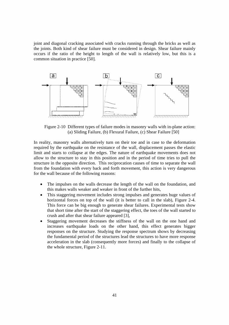
41

joint and diagonal cracking associated with cracks running through the bricks as well as the joints. Both kind of shear failure must be considered in design. Shear failure mainly occurs if the ratio of the height to length of the wall is relatively low, but this is a common situation in practice [50].

Figure 2-10 Different types of failure modes in masonry walls with in-plane action: (a) Sliding Failure, (b) Flexural Failure, (c) Shear Failure [50]

In reality, masonry walls alternatively turn on their toe and in case to the deformation required by the earthquake on the resistance of the wall, displacement passes the elastic limit and starts to collapse at the edges. The nature of earthquake movements does not allow to the structure to stay in this position and in the period of time tries to pull the structure in the opposite direction. This reciprocation causes of time to separate the wall from the foundation with every back and forth movement, this action is very dangerous for the wall because of the following reasons:

• The impulses on the walls decrease the length of the wall on the foundation, and this makes walls weaker and weaker in front of the further hits,

• This staggering movement includes strong impulses and generates huge values of horizontal forces on top of the wall (it is better to call in the slab), Figure 2-4. This force can be big enough to generate shear failures. Experimental tests show that short time after the start of the staggering effect, the toes of the wall started to crush and after that shear failure appeared [3],

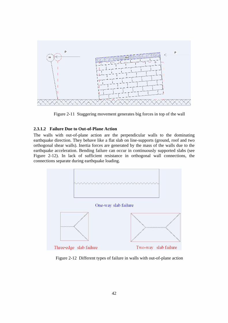
• Staggering movement decreases the stiffness of the wall on the one hand and increases earthquake loads on the other hand, this effect generates bigger responses on the structure. Studying the response spectrum shows by decreasing the fundamental period of the structures lead the structures to have more response acceleration in the slab (consequently more forces) and finally to the collapse of the whole structure, Figure 2-11.

42

Figure 2-11 Staggering movement generates big forces in top of the wall

2.3.1.2 Failure Due to Out-of-Plane Action The walls with out-of-plane action are the perpendicular walls to the dominating earthquake direction. They behave like a flat slab on line-supports (ground, roof and two orthogonal shear walls). Inertia forces are generated by the mass of the walls due to the earthquake acceleration. Bending failure can occur in continuously supported slabs (see Figure 2-12). In lack of sufficient resistance in orthogonal wall connections, the connections separate during earthquake loading.

Figure 2-12 Different types of failure in walls with out-of-plane action

43

2.4 Masonry as a Composite Material Response of masonry structures in earthquakes or generally under any cyclic load depends on their categories; by attention to the type of the masonry structure they have different behavior during cyclic load especially earthquake loading. In general the meaning of masonry structures is kind of the structure that built by construction materials like bricks (burnt brick) or stones plus mortar. There are four types of these structures in main categories:

• Unreinforced structures, • Semi-reinforced structures, • Reinforced structures, • Combined (framed) structures.

Figure 2-13 Composite block masonry structure [49]

Unreinforced structures are the most usual type of masonry structures all around the world. The reason is that it is easy to build with accessible materials that exist in the nature. This type of masonry structures is divided into two types, the first is made of burnt bricks (or pressed brick) and the second type is made of stones. Semi-reinforced masonry structures have the same main structure but the difference is about yoke. Yokes are concrete weak beams or columns that are built in main walls of masonry structures for improvement their behavior especially ductility and tension resistance under loading. Although semi-reinforced structures have better stability during earthquakes, reinforced masonry structures have more advantages as they are completely stable and it is possible to calculate their resistance. A structure with adequate resistance is a structure that has reinforced materials in failure cases. As it is discussed in Section 2.3 masonry walls with regards to in-plane behavior have two cases of failure; shear fracture and flexural fracture. In reinforced masonry structures horizontal reinforcement helps to increase the shear resistance for carrying lateral loads and vertical reinforcement are made for flexural resistance.

44

In combined structure the idea is totally different because on the one hand in this type of masonry the structure is exactly framed, like steel frame or concrete frame, on the other hand this kind of structure could call middle plane (filled) steel or concrete structures. In the case of this research the focus is on the first type of the masonry structure but with new method as it named Gap-Element [44] (see 2.5.2.3). The material property of masonry is the most important part of the masonry research project. Masonry material property is not recognized as the other materials like concrete and steel. There is a gap of specific definition of the material property of any kind of masonry structures. The lack of appropriate knowledge of masonry, made it as a complicated material for modeling. The complex behavior in tension and pressure and nonlinear behavior of masonry are the two faces of the problem. Modeling the masonry as isotropic or anisotropic could be another important part for theoretical modeling of masonry. In the following, different parts of material properties of masonry structures are discussed.

Figure 2-14 Perforated clay blocks of masonry units

2.4.1 Compressive Strength The compressive strength of masonry elements is the strongest point for using masonry, but the tensile strength of masonry always is limiting the usage of masonry. Many traditional masonry buildings were designed using the weight of the floors and the massive walls to prevent tensile stresses caused by eccentricity of vertical loads and by lateral loads. For preventing lateral instability by gravity alone could be a good strategy for traditional masonry buildings but the nature of earthquake-loads and unpredicted behavior of the structure during that loading, caused most of the collapses in the previous earthquake disasters.

45

The strength of masonry is defined by more factors than only the unit and mortar strength. Other factors are [10]:

• Age of the specimen (the curing time of the masonry), • Moisture condition of the unit, • Finishing, • Joint width, • Suction rate of the unit, • Dimensions of the unit (ratio between joint thickness and unit height), • Inner cracks and stresses within the unit, • Craftsmanship of mason, • Filling of the units, • Finishing of the joints.

The clear definition of compressive strength of masonry has to include these two aspects:

• Compressive strength of the units, • Compressive strength of the masonry.

2.4.1.1 Compressive Strength of Units Masonry units can be made of clay, shale, concrete, calcium silicate (or sand lime), stone, and glass, but the most commonly available units are bricks and blocks made clay or concrete. The first step to evaluate the mechanical properties of masonry is to understand the basic properties of the units. Most masonry units are rectangular and lie with long dimension (length) horizontal in the plane of the wall. The exposed vertical surface is the face of the unit and the ends are the vertical faces perpendicular to the plane of the wall. Traditionally, the properties of all masonry units were based on gross area, regardless of the degree to which voids had been incorporated into the units. However, increased sophistication in the structural design methods used to account for slenderness and bending has resulted in the use of the net area of hollow units as the area is effective in resisting various forces. Because masonry is typically designed to resist vertical load, the net area is usually defined as the area of a horizontal section through the unit. Compressive strength of masonry units has been used for a long time as a measure of quality and as a means for predicting other properties such as the compressive strength of masonry assemblages. The masonry unit’s height-to-width ratio can lead to large differences in the apparent compressive strength of the material. This is mainly due to the relative influence of the confining effects of the loading platens of the test machine in laboratory. Under a uni-axial compressive load, materials tend to expand in the transverse directions (Poisson’s effect). Where this expansion is restricted, transverse compressive confining stresses are built up, resulting in a tri-axial compression stress state [12]. The properties of masonry are strongly dependent upon the properties of its constituents. Compressive strength tests are easy to perform and give a good indication of the general quality of the materials used. The CEN Eurocode 6 (1995) uses the compressive strength

46

of the components to determine the strength of masonry even if a true indication of those values is not simple [20]. For masonry units, standard tests with solid plates result in an artificial compressive strength due to the restraint effect of the platens. The CEN Eurocode 6 (1995) minimizes this effect by considering a normalized compressive strength bf , which results from the standard compressive strength, in the relevant direction of the loading, multiplied by an appropriate shape/size factor. The normalized compressive strength refers to a cubic specimen with 100 x 100 x 100 mm3 and can not be considered representative for the true strength. Experiments on the uni-axial post-peak behavior of compressed bricks and blocks are virtually non-existent and no recommendations about the compressive fracture energy fG can be made. It is difficult to relate the tensile strength of the masonry unit to its compressive strength due to the different shapes, materials, manufacture processes and volume of perforations. For the longitudinal tensile strength of clay, calcium-silicate and concrete units, Schubert [23] carried out an extensive testing program and obtained a ratio between the tensile and compressive strength that ranges from 0.03 to 0.1. For the fracture energy fG of solid clay and calcium-silicate units, both in the longitudinal and normal directions, Van Der Pluijim [24] found values ranging from 0.06 to 0.13 N . mm / mm2 for tensile strength values ranging from 1.5 to 3.5 N / mm2.

2.4.1.2 Compressive Strength of Masonry With the modern use of high strength materials and thinner elements, compressive strength is often of prime importance in load bearing structures. Compression tests of masonry prisms are used as the basis for assigning design stress and, in some cases, as a quality control measure. Its importance has made prism compressive behavior a major research focus and potential correlations with other strength characteristics have been investigated. Test machine capacity and specimen height limits as well as other practical considerations have led to use prisms as the main type of compression test specimen rather than full-scale specimens. The bearing capacity of a masonry element subject to compression generally is determined by elastic calculations that take into account the different mechanical properties of the constituents. Compared to experimental checks, these estimates show a systematic error in the order of 50 – 100 %. This is due to the impossibility of defining unequivocally the values of the normal modulus of elasticity and of the transversal contraction coefficient (especially for mortar). These observations suggest that the problem should be approached from a totally different point of view, i. e., not confining the stress analysis to the elastic phase, but taking into account the inelastic phase preceding the rupture [25].

2.4.2 Elastic Moduli Only in the case of purely linear elastic material can be spoken of the elastic modulus. With a nonlinear σ ε− diagram a choice has to be made for a defining method. Since

47

there was a great variation in the strength of the various types of specimens, it has been decided to define the elastic modulus at a load of 35% of the determined fracture load [10]. Some of the researchers suggested 33% for this typical secant modulus of elasticity [12]. The measured force-deformation relation is indicated by a straight line through the origin and the point on the measured force-deformation relation where the force is 35% of the fracture load. The elastic modulus of masonry in the direction perpendicular to the longitudinal joints is ( E⊥ ) lower than the elastic modulus parallel to the longitudinal joints ( //E ), the ratio between these two moduli of elasticity is dependent on the type of masonry. This is the reason why masonry has as an orthotropic behavior. Hamid said: “It is interesting to note that units can be classified as solid based on a 75 % solid bedding area, but have a vertical cross-section less than 75 % solid either in the plane of the wall or through the thickness. This feature is partly responsible for the anisotropic behavior of masonry” [12].

2.4.2.1 Elastic Moduli of Units Because of different types of masonry units that are generated from different factories, it seems to be logic to test units in the laboratory for every study on masonry structures. Elastic modulus of the units as it is explained above is various to different axis. The method is simple, it has to be loaded the units and measure displacement. The generated graphs with explained method give the modulus of elasticity of the units.

2.4.2.2 Stiffness of Masonry Although modulus of elasticity values and stress-strain relationship for masonry assemblages are more useful for design calculations, these properties are often obtained for masonry units in order to provide more complete information on their characteristics. Such information tends to be mainly used in research, but other applications, such as for advanced analytical work, also exist. Because there is no standard method for determining the modulus of elasticity of units, attention should be paid to the applicable stress range. The elastic modulus of the specimen specifies by the below elastic modulus:

• Mortar Elastic Modulus, • Units Elastic Modulus.

The elastic modulus of the mortar is larger when the compressive strength of the units is larger. For finding the stiffness or elastic modulus of masonry, the method is the same for single units. The specimen made of masonry has to be loaded and measure its deformations with the load of 35% of the apparent fracture load.

48

2.4.3 Shear Strength This section discusses the shear strength of masonry elements. Shear failure is a very common failure mode observed in most masonry walls when subjected in-plane loading (Section 2.3). The relationship most commonly adopted to model this phenomenon is a Coulumb - Friction relationship. This is done by means of Mohr-Coulomb’s failure criterion. This assumes that the joint shear strength is composed of an initial strength between the mortar and the masonry unit plus a shear friction capacity, which is considered to be proportional to the compressive stress applied normally to the bed joints. With regard to combined shear and normal stress conditions, this criterion can simply be formulated by:

tan( )cτ ϕ σ= + ⋅ Where: τ = the shear strength, c = the cohesion, ϕ = the angle of internal friction, and σ = the normal stress to the longitudinal joint (tension is negative). The experimental investigations have shown that shear strength corresponding to slip along one or more bed joints, is strongly related to the combined shear and compressive stresses [34], [35]. Then it is apparent that when the shear displacement increases, the cohesion does not suddenly, but more or less gradually decreases to zero. The angle of internal friction is dependent of the material used in masonry body. When the masonry is put in shear, various failure modes can occur [10]:

• Tensile bond failure, • Failure of units, • Failure of masonry in compression, • Failure of the mortar joints.

In masonry, shear walls are intended to resist shear forces from in-plane lateral loads plus the effects of axial load and bending. Depending on the form of construction and the combined effects of axial load and bending, the shear failure mode is characterized by shear slip along the bed joints, diagonal tension cracking, or shear compression failure [32], [33].

2.5 Improvement of Deformation Capacity As it is explained in the previous sections, for overcoming the weak points of masonry structure it has to be focused on ductility. Ductility is the main key to solve this problem, it can be found in different methods. A short description is discussed in the next section.

2.5.1 Capacity Design As the capacity design approach is briefly mentioned, the present chapter is appropriate to this subject, because it is the backbone of the whole research.

49

2.5.1.1 Secure-Roller Criteria One of the most important strategies in earthquake design approach for every engineering structure is stability of the structure in comparison with its resistance against earthquakes. Figure 2-15 shows the difference between stability and resistance. Figure 2-15-I shows an instable structure with sufficient resistance, Figure 2-15-II shows the same structure but with a stable system against earthquakes. The difference between these two structures is related to the method of design and connection performance between the members of the structure for bearing the earthquake load or any kind of cyclic loads. For example strong-column and weak-beam belongs this hypothesis. There are different methods to use this strategy, Gap-Element method is mainly emphasized on this strategy.

displacement

stability level

before earthquake

after earthquake

after earthquakebefore earthquake

stability level

displacement(I) (II)

Figure 2-15 Secure-roller criteria [3]

Secure-ruler criteria [3], is simply focused on the stability and does not allow the external load like earthquake to achieve maximum resistance of the structure. Acceptable displacements will occur in the structure but that does not mean to loose any stability, this permanent or may be returnable displacement is given by ductility.

2.5.1.2 Ductile-Chain Design Criteria The other important strategy that has to be considered in the design of masonry structures is ductile-chain design. Ductile-chain design simply divides the structure in two categories of members: brittle members and ductile members. Amongst the materials used in building construction, steel is ductile, while masonry and concrete are brittle, both masonry and concrete fail suddenly. Considering a structure as a joint of ductile and brittle members, in case of cyclic load the ductile members have to elongate by a large amount before they break, while the brittle members break suddenly on reaching their maximum strength at a relatively small elongation (Figure 2-16).

50

Figure 2-16 Tension test on material, brittle versus ductile materials [19] A simple description of ductile-chain design is to consider a chain with links made of brittle and ductile materials (Figure 2-17). Each of these links will fail just like the different materials shown in Figure 2-16. If force F applies on both ends, this force is being transferred through all the links. The force in each link is the same, i. e., F. While more and more force is applied, eventually the chain will break when the weakest link in it breaks. If the ductile link is the weak one (i. e., its capacity to take load is less), then the chain will show large final elongation. Instead, if the brittle link is the weak one, then the chain will fail suddenly and show small final elongation. Therefore, the backbone of ductile-chain design is based on the design of the ductile link to be the weakest link. The capacity design concept in earthquake-resistant design of buildings will fail if the strengths of the brittle links fall below their minimum assured values. The strength of brittle construction materials, like masonry and concrete, is highly sensitive to the quality of construction materials, workmanship, supervision, and construction methods. Similarly, special care in construction is needed to ensure the elements meant to be ductile are indeed provided with features that give adequate ductility. Buildings should be designed like the ductile chain. For example, strong-column weak-beam design method is established from this strategy of design, but for masonry this strategy has to be satisfied with another method. By using the routine design codes (meant for design against non-earthquake effects), designers may be unable to achieve a ductile structure. Special design provisions are required to help designers to improve the ductility of the structure. Such provisions are usually put together in the form of a special seismic design code. These codes also ensure that adequate ductility is provided in the members where damage is expected.

51

Figure 2-17 Ductile-Chain design [19]

2.5.2 Methods for Improving Deformation Capacity of Masonry There are many different methods to improve deformation capacity of masonry structures. In the following are some famous methods for improving the masonry behavior during the cyclic load especially their usage in retrofit and rehabilitation or as a new construction method described.

2.5.2.1 C.F.R.P Sheets Masonry structures may need strengthening for a variety of reasons. For example creep within the structure may redistribute loads such that the masonry is carrying more loads over time. This may occur from increasing deformations elsewhere in the structure or from redistribution of stress within a structural element itself. If load redistribution to masonry is combined with a reduction in strength from external environmental factors such as weathering, then increasing load with decreasing strength over time can lead to failure. This for example is the probable cause of the collapse of the Civic Tower of Pavia. Many masonry buildings constituting artistic and architectural heritage often need retrofit or strengthening interventions and the use of the technique of FRP (Fiber Reinforced Polymer) laminates glued with epoxy resin appears adequate because of the lightness, the easiness of application, and the possibility of removal. This reinforcing technique has been a topic of studies over the past ten years [37]. This advanced polymer matrix fibrous composite material was developed for high-performance aircraft but it can offer major advantages for repair and retrofitting of masonry construction through external bonding of thin composite strips and sheets. Worldwide a great number of masonry structures are located in seismically endangered regions. The earthquake forces occurring in the bearing structures must often be transferred through the masonry into the foundations. However, the masonry walls, which are loaded by shearing and bending forces, often do not meet the needed requirements. Methods were developed in use of FRP or CFRP (Carbon Fiber Reinforced Polymer) could be as an effective solution to overcome such kind of weak points of masonry structures.

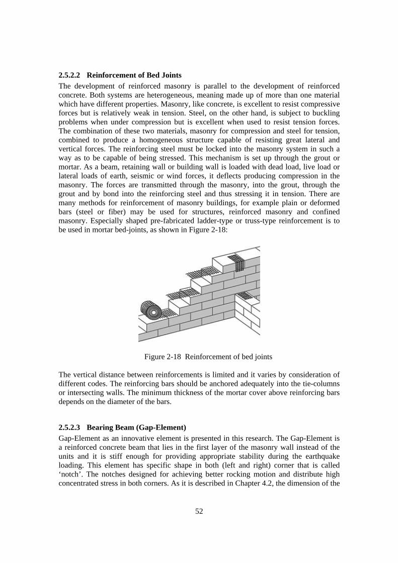
52

2.5.2.2 Reinforcement of Bed Joints The development of reinforced masonry is parallel to the development of reinforced concrete. Both systems are heterogeneous, meaning made up of more than one material which have different properties. Masonry, like concrete, is excellent to resist compressive forces but is relatively weak in tension. Steel, on the other hand, is subject to buckling problems when under compression but is excellent when used to resist tension forces. The combination of these two materials, masonry for compression and steel for tension, combined to produce a homogeneous structure capable of resisting great lateral and vertical forces. The reinforcing steel must be locked into the masonry system in such a way as to be capable of being stressed. This mechanism is set up through the grout or mortar. As a beam, retaining wall or building wall is loaded with dead load, live load or lateral loads of earth, seismic or wind forces, it deflects producing compression in the masonry. The forces are transmitted through the masonry, into the grout, through the grout and by bond into the reinforcing steel and thus stressing it in tension. There are many methods for reinforcement of masonry buildings, for example plain or deformed bars (steel or fiber) may be used for structures, reinforced masonry and confined masonry. Especially shaped pre-fabricated ladder-type or truss-type reinforcement is to be used in mortar bed-joints, as shown in Figure 2-18:

Figure 2-18 Reinforcement of bed joints The vertical distance between reinforcements is limited and it varies by consideration of different codes. The reinforcing bars should be anchored adequately into the tie-columns or intersecting walls. The minimum thickness of the mortar cover above reinforcing bars depends on the diameter of the bars.

2.5.2.3 Bearing Beam (Gap-Element) Gap-Element as an innovative element is presented in this research. The Gap-Element is a reinforced concrete beam that lies in the first layer of the masonry wall instead of the units and it is stiff enough for providing appropriate stability during the earthquake loading. This element has specific shape in both (left and right) corner that is called ‘notch’. The notches designed for achieving better rocking motion and distribute high concentrated stress in both corners. As it is described in Chapter 4.2, the dimension of the

53

Gap-Element is calculated by SAP2000.The Corner-Gap-Element is a way to improve the deformation capacity of masonry walls. The main idea is based on the weak point of masonry structures: the corner points of walls during an earthquake. Figure 2-19 explains the main idea of the Corner-Gap-Element and the way of loading of masonry walls that in most cases leads to a high exploitation of the shear capacity. Since the bending moments increase with shear forces, the eccentricity of the normal force in the critical cross section becomes significant. This in turn leads to a reduction of the size of the compression zone in unreinforced walls with high concentration of normal stresses and shear stresses. In order to overcome this problem, Corner-Gap-Elements, enabling the transfer of the capacity design concept to unreinforced masonry have been proposed. These elements, consisting of a bearing beam made of a sufficient strong material (such as reinforced concrete), ensure a limitation of eccentricity of the normal force (see Section 7.4.2) and thus, restrict the pinching of the compression zone. The deformation can be concentrated in the joint below the bearing beam. The masonry itself is protected from high stresses as a potential cause of brittle failure (ductile-chain design, Section 2.5.1.2). In this way, the principles of capacity design can be transferred to masonry structures. Numerical modeling of masonry walls with Corner-Gap-Elements has confirmed the principles that are laid down in the previous section [4]. An experimental proof of the validity of the proposed capacity design approach for masonry with Corner-Gap-Elements, however, has been missing up to now.

Figure 2-19 Corner-Gap-Element in masonry walls

54

3 ANALYTICAL MODELING OF MASONRY STRUCTURES

3.1 Introduction “In the finite element method a structure is subdivided into a number of separate ‘elements’, each of them with certain properties. The method suits masonry extremely well because the elements already present by nature in the form of units or blocks”. J.G.Rots [10]. The complexity of masonry structure behavior and the fact that different methods lead to differences in the results, always make difficulties on the research of masonry structures. Objective of this chapter is to show a simple method for modeling the tested masonry structure with reasonable time-cost. The method discusses the Homogenous-Modeling of the masonry and includes details of the whole structure’s elements according to their role in the load bearing system. The best method for the modeling of masonry structures respectively with its complexity is the method which seeks information with a reliable manner. The method has to prove acceptable errors compared with the listed costs. Reliable numerical analyses can be achieved only with the correct mechanical properties, which are obtained serious experiments. Therefore it is role of tomb to do various tests on masonry to have good computer simulations. The current numerical analyses software (tools) does not have the desired ability level. Generally, the simulation of masonry can be performed by using mechanics of granular materials such as concrete and rock. The finite element of masonry could contain two groups of modeling. The first group is Heterogeneous-Modeling and the second group is Homogeneous-Modeling. These two categories are approximately similar to the definition of macro and micro modeling. In Heterogeneous-Modeling units and mortar introduce separately to the program and the usage of this approach is useful for small scale modeling, but Homogenous-Modeling considers units and mortar as a compound material and their mechanical properties introduce as a single material. It is possible in Homogenous–Modeling to apply the model as an isotropic or anisotropic model. Heterogeneous-Modeling is not interested in the field of masonry. Large scale structures and the limited abilities of computers for running such kind of model, limit this kind of approach for small models only. In this modeling it is necessary to have test results of large masonry parts that contain adequate unit and mortar combinations. The Homogeneous-Modeling approach can be applied for large scale structures. Macro-models and micro-models are useable for different purposes of the modeling. For example macro-model is faster to analyze and easier to settle in computer but accuracy is

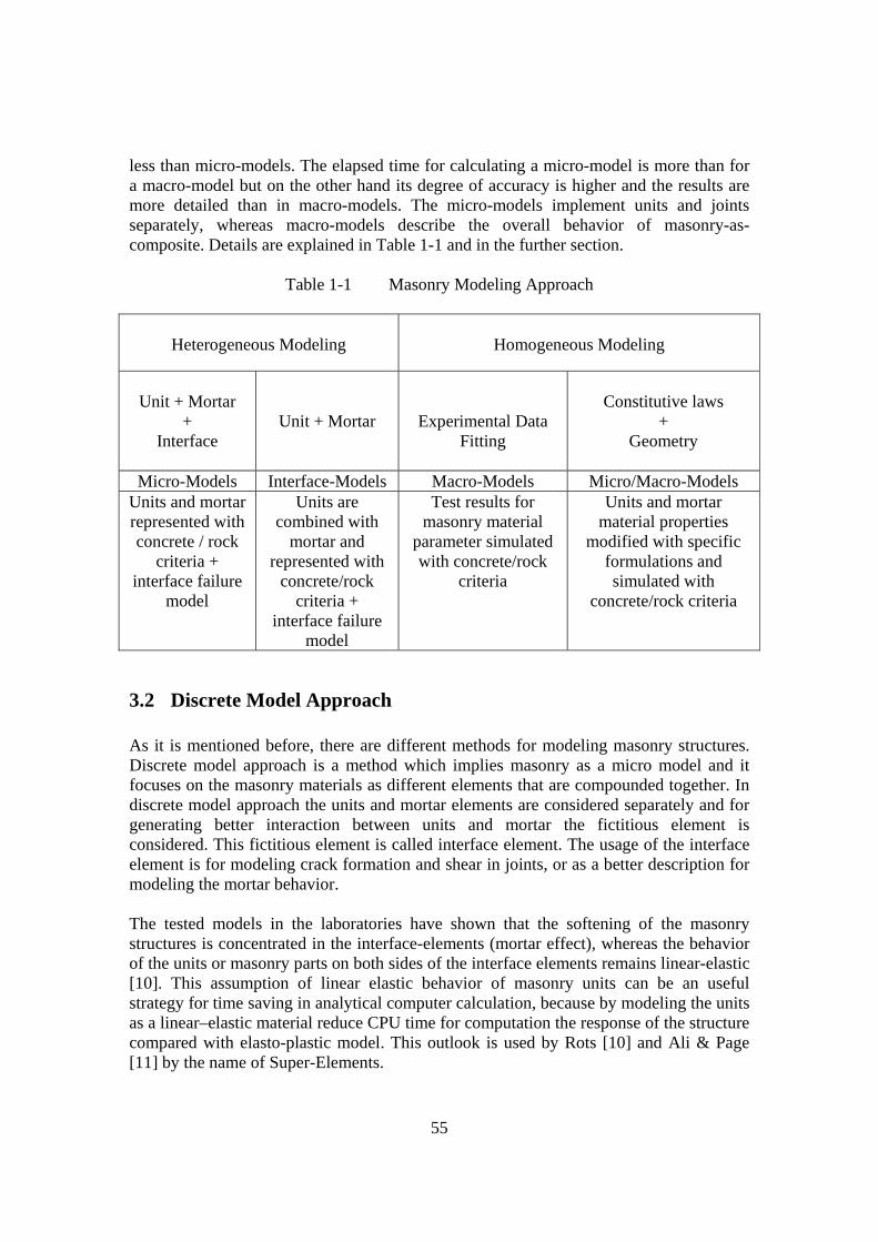
55

less than micro-models. The elapsed time for calculating a micro-model is more than for a macro-model but on the other hand its degree of accuracy is higher and the results are more detailed than in macro-models. The micro-models implement units and joints separately, whereas macro-models describe the overall behavior of masonry-as-composite. Details are explained in Table 1-1 and in the further section.

Table 1-1 Masonry Modeling Approach

Heterogeneous Modeling

Homogeneous Modeling

Unit + Mortar

+ Interface

Unit + Mortar

Experimental Data Fitting

Constitutive laws

+ Geometry

Micro-Models Interface-Models Macro-Models Micro/Macro-Models Units and mortar represented with concrete / rock

criteria + interface failure

model

Units are combined with

mortar and represented with

concrete/rock criteria +

interface failure model

Test results for masonry material

parameter simulated with concrete/rock

criteria

Units and mortar material properties

modified with specific formulations and simulated with

concrete/rock criteria

3.2 Discrete Model Approach As it is mentioned before, there are different methods for modeling masonry structures. Discrete model approach is a method which implies masonry as a micro model and it focuses on the masonry materials as different elements that are compounded together. In discrete model approach the units and mortar elements are considered separately and for generating better interaction between units and mortar the fictitious element is considered. This fictitious element is called interface element. The usage of the interface element is for modeling crack formation and shear in joints, or as a better description for modeling the mortar behavior. The tested models in the laboratories have shown that the softening of the masonry structures is concentrated in the interface-elements (mortar effect), whereas the behavior of the units or masonry parts on both sides of the interface elements remains linear-elastic [10]. This assumption of linear elastic behavior of masonry units can be an useful strategy for time saving in analytical computer calculation, because by modeling the units as a linear–elastic material reduce CPU time for computation the response of the structure compared with elasto-plastic model. This outlook is used by Rots [10] and Ali & Page [11] by the name of Super-Elements.

56

The discrete (distinct) model was proposed by Cundall [26] for the study of jointed rock, modeled as an assemblage of rigid blocks. Later, this approach was extended to other fields of engineering, where the detailed study of joints is required, e. g. soils and other granular materials [27]. This numerical technique has also been used for the modeling of masonry structures, where good quality results have been achieved (see Figure 3-1 and [28], [29], [30]).

Figure 3-1 Analysis of masonry structures using the discrete element method:

(a) masonry arch bridge [29], (b) dry stone masonry pedestal sustaining a status [21]

Within the discrete element method, blocks can be considered both rigid and deformable. For the structures where relative low stresses and deformations occur in the blocks, the hypothesis of un-deformable blocks is rather realistic. Also the consideration of the block deformability approaches discrete element method and discontinuous finite element method. Apart from solution techniques, the main difference between these two methods lies in the modeling of contact: discontinuous finite element, models use interface elements and discrete elements models are based on a point contact approach [29], i. e. at the interfaces the blocks are connected by means of contact points, since discrete element models are intended to simulate the large displacement range. In discrete model approach, micro-model is the basic criteria for modeling, Table 1-1. Micro-models are, probably the best available tool to understand the behavior of masonry. The benefit of using such an approach is that all the different failure mechanisms can be considered. In this method attention is given to a simplified modeling strategy, in which interface elements are used as a potential crack, slip or crushing planes. The assumption is that all of the inelastic phenomena occur in the interface elements which lead to a robust type of modeling, capable of following the complete load path of a structure until load degradation of stiffness. The fact that little importance has been given to numerical modeling of masonry is confirmed by the absence of any well established micro-model.

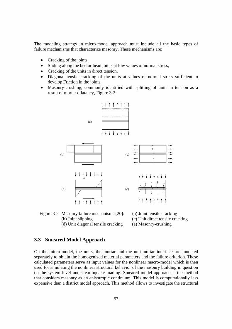
57

The modeling strategy in micro-model approach must include all the basic types of failure mechanisms that characterize masonry. These mechanisms are:

• Cracking of the joints, • Sliding along the bed or head joints at low values of normal stress, • Cracking of the units in direct tension, • Diagonal tensile cracking of the units at values of normal stress sufficient to

develop Friction in the joints, • Masonry-crushing, commonly identified with splitting of units in tension as a

result of mortar dilatancy, Figure 3-2:

Figure 3-2 Masonry failure mechanisms [20]: (a) Joint tensile cracking (b) Joint slipping (c) Unit direct tensile cracking (d) Unit diagonal tensile cracking (e) Masonry-crushing

3.3 Smeared Model Approach On the micro-model, the units, the mortar and the unit-mortar interface are modeled separately to obtain the homogenized material parameters and the failure criterion. These calculated parameters serve as input values for the nonlinear macro-model which is then used for simulating the nonlinear structural behavior of the masonry building in question on the system level under earthquake loading. Smeared model approach is the method that considers masonry as an anisotropic continuum. This model is computationally less expensive than a district model approach. This method allows to investigate the structural

58

behavior of large substructures subject to dynamic loading. In order to use this method, the effective stiffness of masonry and the smeared nonlinear characteristics must be known, requiring the definition of stress-strain relationships for monotonic and cyclic loading. In addition, the global failure criterion has to be defined [31]. Smeared model approach actually is macro-model approach. Smeared model approach has other aspects by using in practice, for example in smeared model approach some failure modes cannot be captured, due to simplicity of the modeling. The accuracy of this type of modeling strongly depends on the number of meshes generation. In case of finer mesh the accuracy is higher than of coarser mesh but the time-charge is bigger.

Figure 3-3 Modeling strategy for masonry:

(a) Masonry sample (b) Detailed micro-modeling (c) Simplified micro-modeling (d) Macro-modeling

The disadvantage of this modeling is about the lack of any pattern of failure in mortar and units connection points but on the other hand this kind of modeling can give maximum response of the whole masonry body. For such explained reasons the localized effects cannot be captured. There are still not completely proved yield surface plastic models for anisotropic macro masonry models. Therefore it is necessary to use yield surface models of granular structures for macro masonry modeling. For material property data input comprehensive testing results are needed to determine the assembling property of the masonry body (units and mortar) under different types of loading. Finite element method is still young enough for generating good results in the field of analyzing masonry structures, especially in smeared model approach, because of the complexity of masonry and no well defined constitutive law for the stress-strain curve and failure simulation of masonry. There are other extra options that make analyzing of masonry more complicated, for example; geometrical details of many existing masonry structures are

59

very complicated and in dynamic simulation the number of unknowns is increasing due to non-linear changes of masonry during vibration.

60

4 OPTIMIZATION OF GAP-ELEMENT GEOMETRY

4.1 Introduction This chapter is appropriated to numerical investigation for calculating the dimensions of Gap-Element. In order to optimize the dimensions of Gap-Element the finite element software SAP2000 have been performed. This software could generate good results to find out the right dimension of the Gap-Element and the model is analyzed with linear-elastic approach.

4.2 Optimization Procedures Gap-Element has to be defined by its dimension. Gap-Element’s dimensions are specified by dimensions in three axes (length, height and thickness) and also the notch dimensions have to be clarified. The length and thickness of the Gap-Element adopt from the masonry wall above the Gap-Element. The length of the Gap-Element and its thickness are equal to the length of the wall and the thickness of the units. The height of the Gap-Element and the geometry of the notches must be calculated with appropriate assumptions by analytical calculation. The notch dimensions are the most important size evaluation of the Gap-Element, because workability of the Gap-Element depends on the size of the notch (length and height of the notch). The height of the notches is also noticeable but not as much as the length of the notches and their heights are considered only for providing an untouchable surface below the notch with the foundation during the rocking motion of the Gap-Element. The height of the notches for all tests is 2 cm. As it is observed in laboratory on the shaking table, the Gap-Element could overcome to produce rocking motion with this height of the notches. The only sizes that have to be calculated are the height of the Gap-Element and length of the notches. SAP2000 has been selected for evaluating the height of the Gap-Element and the length of the notches. The material property is based on the linear-elastic approach, because linear-elastic approach gives sufficient information about the distribution of the stress above the Gap-Element. Smeared model approach and achieve to simple calculations could produce tension distribution above the Gap-Element in the units. Several trial and errors on Gap-Element’s dimensions (height and notch’s length) and different type of mesh generation finally produced the right values for height of the Gap-Elements and length of the notches Figure 4-1:

61

Figure 4-1 Gap-Element on the shaking table and under the wall specimen #3, dimensions in millimeter

This theoretical method is based on the recommended load (vertical and horizontal) according to the DIN-1055 [45] and produced stresses on the normal masonry wall. Figure 4-2 shows the shear distribution on this normal masonry wall under the load conditions of the one wall in first specimen (more details are available in the table C-4 in Appendix - C): Total weight of the first specimen = 192 kN, V= 192 / 2 = 96 kN and N= 0.25 x V = 24 kN. As it is shown in this figure the shear stress is increasing strongly near the edge (as it is expected for the uplift that caused by lateral force). Overturning moment that is made by lateral force will compel the structure to stand up around one edge, this asymmetric uplift generates high values of shear and compressive stresses around this edge (consequently in reciprocation movement the other edge experiences same effect, see Figure 2-11 for more detail). The shear stress at the edges of the wall will capture its maximum values. Figure 4-3 shows the same wall (geometry and loading) in the Figure 4-2 but with the Gap-Element. Many times trial and errors are confirmed that the notch’s length around 17 cm has the best shear and compressive stress distribution not only above the Gap-Element (in first brick layer) but also below the Gap-Element around the edges, consequently the height of the Gap-Element has to be specified as a last parameter of Gap-Element’s dimension. Figure 4-3 is cumulative results of these trial and errors for best selection of the Gap-Element’s height with the specified length of the notches = 17 cm. There are three types of the height are shown in Figure 4-3; 15 cm, 20 cm and 25 cm.

62

As it realizes from these calculations the compatible size with the brick dimension in vertical course (height of the brick plus mortar’s thickness is 25 cm) is the best selection for the Gap-Element height, because it has smoother shear stress distribution on the edges of the masonry wall (in Figure 4-3 the shear stress distribution after x > 40 cm continued with same values and decreased to the zero after reaching the uplift area caused by overturning moment).

-200

0

200

400

600

800

1000

1200

0510152025303540

X [ cm ]

Shea

r Str

ess

[ kN

/ m

² ]

Figure 4-2 Shear stress distribution in normal masonry walls during the normal

loading (horizontal and vertical)

Shear Stress Distribution in the Masonry Wall with Gap-Element (Notch's Length = 17 cm)

-150

-100

-50

0

50

100

150

200

250

300

350

400

0481216202428323640

X [ cm ]

Shea

r Str

ess

[ kN

/ m

² ]

Height Beam 15 cm

Height Beam 20 cm

Height Beam 25 cm

Figure 4-3 Shear stress distribution under the masonry wall above the Gap-

Element for different types Gap-Element’s height with the notch’s length = 17 cm along X axis

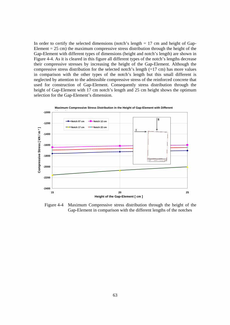
63

In order to certify the selected dimensions (notch’s length = 17 cm and height of Gap-Element = 25 cm) the maximum compressive stress distribution through the height of the Gap-Element with different types of dimensions (height and notch’s length) are shown in Figure 4-4. As it is cleared in this figure all different types of the notch’s lengths decrease their compressive stresses by increasing the height of the Gap-Element. Although the compressive stress distribution for the selected notch’s length (=17 cm) has more values in comparison with the other types of the notch’s length but this small different is neglected by attention to the admissible compressive stress of the reinforced concrete that used for construction of Gap-Element. Consequently stress distribution through the height of Gap-Element with 17 cm notch’s length and 25 cm height shows the optimum selection for the Gap-Element’s dimension.

-2400

-2200

-2000

-1800

-1600

-1400

-1200

-1000

15 20 25Height of the Gap-Element [ cm ]

Com

pres

sive

Str

ess

[ kN

/ m

² ]

Notch 07 cm Notch 12 cm

Notch 17 cm Notch 22 cm

Maximum Compressive Stress Distribution in the Height of Gap-Element with Different Di i

Figure 4-4 Maximum Compressive stress distribution through the height of the

Gap-Element in comparison with the different lengths of the notches

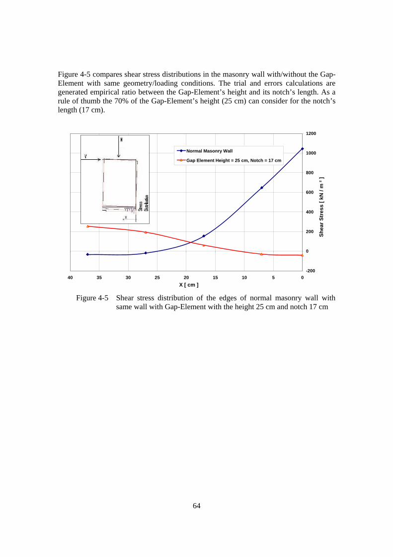
64

Figure 4-5 compares shear stress distributions in the masonry wall with/without the Gap-Element with same geometry/loading conditions. The trial and errors calculations are generated empirical ratio between the Gap-Element’s height and its notch’s length. As a rule of thumb the 70% of the Gap-Element’s height (25 cm) can consider for the notch’s length (17 cm).

-200

0

200

400

600

800

1000

1200

0510152025303540X [ cm ]

Shea

r Str

ess

[ kN

/ m

² ]

Normal Masonry Wall

Gap Element Height = 25 cm, Notch = 17 cm

Figure 4-5 Shear stress distribution of the edges of normal masonry wall with

same wall with Gap-Element with the height 25 cm and notch 17 cm

65

5 EXPERIMENTAL TESTS WITH SHAKING TABLE

5.1 Introduction Experimental investigations were conducted in earthquake laboratory of NTUA (National Technical University of Athens). The masonry units (clay bricks) and some other basic materials were transferred from Germany to Greece. NTUA earthquake laboratory has modern facilities and skilled personnel for checking which kind of earthquake tests as our test. Appendix - B describes technical specifications of earthquake laboratory in NTUA. The experimental investigations were included three specimens with various specifications that are described in details in Section 5.3 and Appendixes A and C. The entire series of tests has been conducted within 2 months after transferring the materials and in order to economize, the roofs of specimen #1 reused for specimen #3. Detail of load specification is described in the Section 5.2. The load introduced to the shaking table as a time-history data input. Section 5.4 and further sections explain observations during the experimental tests and data processing of the specimens.

5.2 Loading Specifications Earthquake design codes typically define the loading by response spectra. For the experimental investigations, we selected the response spectrum for soil conditions A2 according to the draft of the German earthquake code DIN 4149 available at the time of the beginning of the tests (see Figure 5-1). The soil conditions A2 reflect a situation where the rock defines the geological soil conditions superseded by a layer of sandy soil or gravel (geotechnical soil conditions).

66

Figure 5-1 Elastic design spectrum type-A2 according of DIN-4149 [52]

In the Earthquake Laboratory of N.T.U.A (for more detail see Appendix - B), an artificial time record has been generated on the basis of the given response spectrum and assuming an seismic event of short duration with about 5 seconds as it has to be expected for e.g. Germany (see Figure 5-2). This reflects the shallow sources for earthquakes in Central Europe. The total duration of the time-history took 5.12 s.

Table Excitation (Time - History )

-0.8

-0.6

-0.4

-0.2

0

0.2

0.4

0.6

0.8

0 0.5 1 1.5 2 2.5 3 3.5 4 4.5 5 5.5

Time [ sec ]

Acc

eler

atio

n [ m

/ se

c² ]

Figure 5-2 Shaking table input data (time-history)

67

From the specified time-history, response spectra have been obtained for different degrees of structural damping as shown in Figure 5-3. It should be noted, that a modification of the table input data became necessary in order to avoid to exceed the table deformation capacity during the last loading steps for the third specimen. This is discussed in detail in Appendix - D.

Response Spectrum of Time History

0

0.5

1

1.5

2

2.5

3

3.5

4

4.5

5

5.5

6

0 0.2 0.4 0.6 0.8 1 1.2 1.4 1.6 1.8 2T [sec]

Acc

eler

atio

n [m

/sec

²]

Damping 0.00

Damping 0.01

Damping 0.02

Damping 0.05

Damping 0.10

Figure 5-3 Response spectrum of the selected time-history

The loading acted individually. For every test specimen the loading increment was equal and with the same time-history and data input. Random test was before starting every sequence of loading, the random test specified the fundamental frequency of the structure for data processing and theoretical research. The Table 5-1 contains two different types of information for every specimen; first it shows the fundamental frequency of the structure that is gained by random test results and second the P.T.A. (Peak Table Acceleration) acted on the structure. In order to compare the ability of Gap-Element to bear more value of excitation, all test specimen input data gathered in this table. The table shows clearly the Gap-Element could approximately resist with two times P.T.A. more than first specimen. The data processing in further sections shows the details. Maximum excitation rate for random test was about 0.25 m/s2.

68

Table 5-1 Shaking table individual input file for test specimens

Test Number

Test Criteria

Output

Spec. #1

Spec. #2

Spec. #3

1 Random Test F.F.*[Hz] 5.66 6.93 6.65 2 Earthquake Test P.T.A.**[m/s2] 0.599 0.588 0.542 3 Random Test F.F. [Hz] 5.47 6.93 6.65 4 Earthquake Test P.T.A. [m/s2] 0.905 0.923 0.784 5 Random Test F.F. [Hz] 5.37 6.93 6.65 6 Earthquake Test P.T.A. [m/s2] 1.208 1.173 1.064 7 Random Test F.F. [Hz] 5.37 6.93 6.65 8 Earthquake Test P.T.A. [m/s2] 1.605 1.562 1.552 9 Random Test F.F. [Hz] 5.17 6.93 6.65 10 Earthquake Test P.T.A. [m/s2] 2.197 2.292 3.304 11 Random Test F.F. [Hz] 5.17 6.93 6.60 12 Earthquake Test P.T.A. [m/s2] 3.183 3.643 2.999 13 Random Test F.F. [Hz] 5.08 6.93 6.60 14 Earthquake Test P.T.A. [m/s2] 2.987 3.832 3.485 15 Random Test F.F. [Hz] 5.08 6.93 6.15 16 Earthquake Test P.T.A. [m/ s2] 4.335 4.221 3.833 17 Random Test F.F. [Hz] 5.08 6.93 6.15 18 Earthquake Test P.T.A. [m/s2] 4.226 4.437 4.27 19 Random Test F.F. [Hz] 4.88 6.93 5.76 20 Earthquake Test P.T.A. [m/s2] 4.907 4.744 5.096 21 Random Test F.F. [Hz] 4.69 6.65 5.76 22 Earthquake Test P.T.A. [m/s2] 5.394 5.89 6.431 23 Random Test F.F. [Hz] 4.49 - 5.76 24 Earthquake Test P.T.A. [m/s2] - - 6.209 25 Random Test F.F. [Hz] - - 5.76 26 Earthquake Test P.T.A. [m/s2] - - 8.675 27 Random Test F.F. [Hz] - - 5.70 28 Earthquake Test P.T.A. [m/s2] - - 7.937 29 Random Test F.F. [Hz] - - 5.65 30 Earthquake Test P.T.A. [m/s2] - - 9.093 31 Random Test F.F. [Hz] - - 5.60 32 Earthquake Test P.T.A. [m/s2] - - 10.614 33 Random Test F.F. [Hz] - - 5.18 34 Earthquake Test P.T.A. [m/s2] - - 12.031

* F.F.: Fundamental Frequency ** P.T.A.: Peak Table Acceleration (recorded by installed accelerometer on shaking- table)

69

5.3 Experimental Investigation The table excitation followed the synthetic time-history as documented previously. It has been applied several times with increasing intensity. It should be noted, that the acceleration values given here as nominal input data correspond to the ground acceleration on rocky soil. The maximum acceleration values should be 25% higher according to a soil factor of S = 1.25 for soil type-A2. Actually, the real measured values differ from this factor. In most cases, somewhat higher values have been recorded. Observations describe the behavior of specimens during the test when the structure excited with the explained time-history in Section 5.2. In these three tests entire excitation in every dynamic test on the specimens was 5.12 s except the last three tests in specimen #3. Then this is short time but many important scientific information could be receive, further sections describe entire observations for three specimens. Here, two type of excitation is meaning, as follows:

1. Table calibrated excitation for example 40%g (g means gravity acceleration), 2. Real value that acted on the structure for example 5 m/s2.

Difference between of these two values related about the excitation that table calibrated, increased of some effects, for example maybe hydraulic pumps, or resonance effect etc. Real value that must consider in calculation is acceleration data recorded by computer during the test that is normally bigger than calibrated excitation value. Then when it is referred %g means calibrated excitation of the shaking table and when is referred m/s2 it means the real maximum acceleration value of the shaking table.

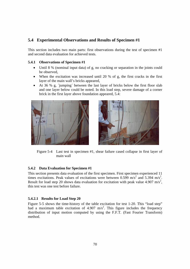
70

5.4 Experimental Observations and Results of Specimen #1 This section includes two main parts: first observations during the test of specimen #1 and second data evaluation for achieved tests.

5.4.1 Observations of Specimen #1 • Until 8 % (nominal input data) of g, no cracking or separation in the joints could

be observed, • When the excitation was increased until 20 % of g, the first cracks in the first

layer of the main wall’s bricks appeared, • At 36 % g, ´jumping´ between the last layer of bricks below the first floor slab

and one layer below could be noted. In this load step, severe damage of a corner brick in the first layer above foundation appeared, 5.4:

Figure 5-4 Last test in specimen #1, shear failure cased collapse in first layer of main wall

5.4.2 Data Evaluation for Specimen #1 This section presents data evaluation of the first specimen. First specimen experienced 11 times excitations. Peak values of excitations were between 0.599 m/s2 and 5.394 m/s2. Result for load step 20 shows data evaluation for excitation with peak value 4.907 m/s2, this test was one test before failure.

5.4.2.1 Results for Load Step 20 Figure 5-5 shows the time-history of the table excitation for test 1-20. This “load step” had a maximum table excitation of 4.907 m/s2. This figure includes the frequency distribution of input motion computed by using the F.F.T. (Fast Fourier Transform) method.

71

Figure 5-5 Table excitation and its FFT-spectrum, load step 20

Horizontal roof responses have been recorded in main and lateral direction. Figure 5-6 shows roof responses in main direction, as it is expected in this figure second roof has higher values of responses in comparison with the first roof, it means, the structure experienced first mode. Spectra are calculated and shown in Figure 5-7; the calculated spectra shows that the most achieved frequencies are around the 3 Hz.

Figure 5-6 Responses of four points in both roofs, load step 20

72

Transfer functions of the roofs are shown in Figure 5-8; these transfer function are generated to evaluate the responses of the structure related to the table excitation. Compatibility between the prevailing frequency of the table excitation (around 3 Hz, see Figure 5-5) with the prevailing response frequencies of the roof (around 3 Hz) means that the structure was in resonance domain. The prevailing frequency of the roof responses (3 Hz) in comparison with the fundamental frequency of the structure before excitation (5.65 Hz, see Appendix - C, Table C-4) is related to the nonlinear behavior of the structure during the high values of the table excitation in last tests.

Figure 5-7 Spectra of roof responses, load step 20

Figure 5-8 Transfer-functions of four points, load step 20

73

Figure 5-9 shows shear forces for second roof versus the displacement in the center of the roof (in the following being addressed as average displacement). The figure shows that nonlinear behavior becomes effective during the time-history of this load step.

Specimen #1, Top Story Test (20)

-40

-30

-20

-10

0

10

20

30

40

-10 -5 0 5 10 15 20 25Displacement 2-Floor [mm]

Shea

r For

ce in

2-F

loor

[kN

]

Figure 5-9 Second floor shear force vs. displacement, load step 20

The fundamental frequency of the tested structure has been identified subsequently to each load step by applying a random signal (white noise type) of small amplitude to the shaking table. From the transfer-function, which in any case is required for optimization of the control signal of the table, the fundamental frequency of the structure has been computed. Because of cracking and failure in some positions of the structure, the stiffness of the structure decreased, and as a result, the fundamental frequency during the course of the testing is reduced. Figure 5-10 shows the fundamental frequencies as obtained from random excitation for all load steps for specimen #1.

74

Specimen #1

0

1

2

3

4

5

6

7

0.5 1 1.5 2 2.5 3 3.5 4 4.5 5 5.5

Maximum Table Excitation [m/sec²]

Fund

amen

tal F

requ

ency

of

the

Stru

ctur

e [H

z]

Figure 5-10 Fundamental frequency reduction (random-test result), specimen #1

Figure 5-8 shows maximum roof responses vs. maximum roof horizontal displacement for specimen #1. Nonlinear behavior of the structure is evident.

Specimen #1

0

1

2

3

4

5

6

7

8

9

2.5 5 7.5 10 12.5 15 17.5 20 22.5 25 27.5 30Maximum Roofs Displacement [ mm ]

Max

imum

Roo

f Res

pons

es [

m /

s ² ]

First Floor Response

Second Floor Response

Figure 5-11 Maximum roof responses vs. maximum roof horizontal displacement,

specimen #1

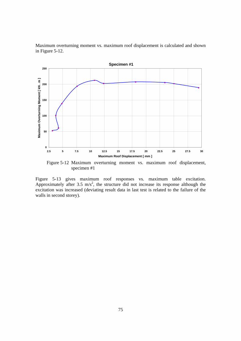
75

Maximum overturning moment vs. maximum roof displacement is calculated and shown in Figure 5-12.

Specimen #1

0

50

100

150

200

250

2.5 5 7.5 10 12.5 15 17.5 20 22.5 25 27.5 30

Maximum Roof Displacement [ mm ]

Max

imum

Ove

rtur

ning

Mom

ent [

kN

. m

]

Figure 5-12 Maximum overturning moment vs. maximum roof displacement,

specimen #1 Figure 5-13 gives maximum roof responses vs. maximum table excitation. Approximately after 3.5 m/s2, the structure did not increase its response although the excitation was increased (deviating result data in last test is related to the failure of the walls in second storey).

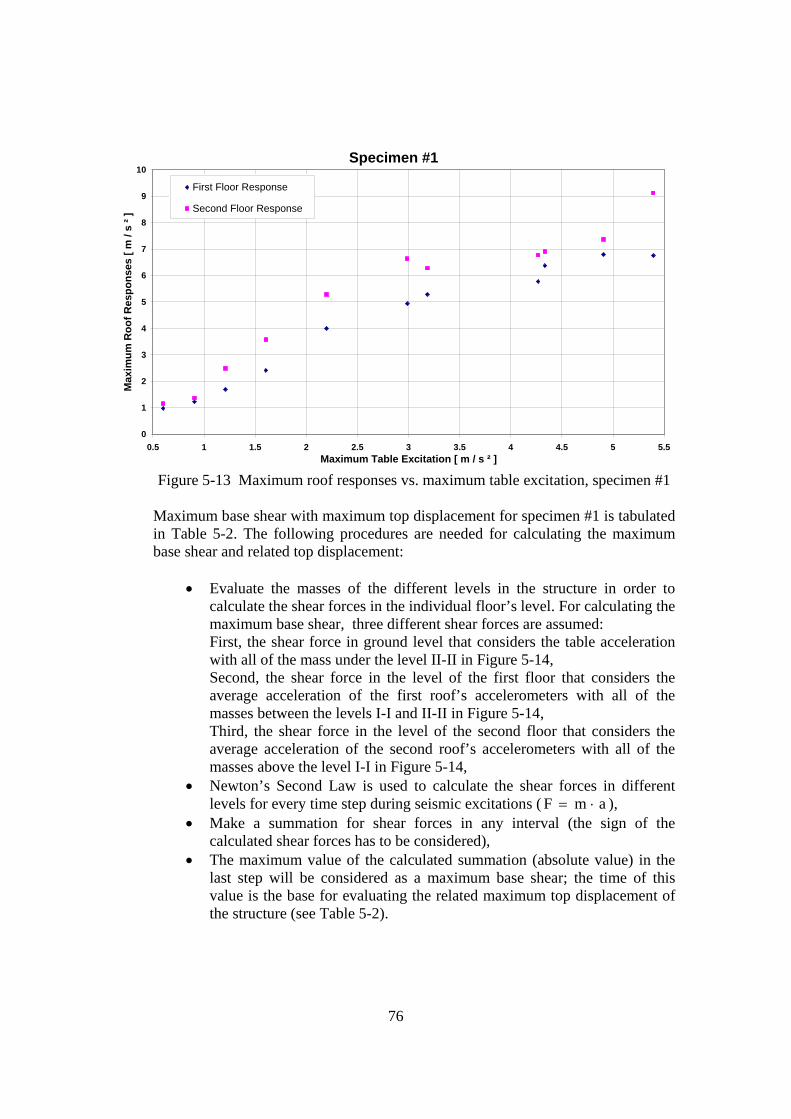
76

Specimen #1

0

1

2

3

4

5

6

7

8

9

10

0.5 1 1.5 2 2.5 3 3.5 4 4.5 5 5.5Maximum Table Excitation [ m / s ² ]

Max

imum

Roo

f Res

pons

es [

m /

s ² ]

First Floor Response

Second Floor Response

Figure 5-13 Maximum roof responses vs. maximum table excitation, specimen #1

Maximum base shear with maximum top displacement for specimen #1 is tabulated in Table 5-2. The following procedures are needed for calculating the maximum base shear and related top displacement:

• Evaluate the masses of the different levels in the structure in order to calculate the shear forces in the individual floor’s level. For calculating the maximum base shear, three different shear forces are assumed: First, the shear force in ground level that considers the table acceleration with all of the mass under the level II-II in Figure 5-14, Second, the shear force in the level of the first floor that considers the average acceleration of the first roof’s accelerometers with all of the masses between the levels I-I and II-II in Figure 5-14, Third, the shear force in the level of the second floor that considers the average acceleration of the second roof’s accelerometers with all of the masses above the level I-I in Figure 5-14,

• Newton’s Second Law is used to calculate the shear forces in different levels for every time step during seismic excitations ( F m a= ⋅ ),

• Make a summation for shear forces in any interval (the sign of the calculated shear forces has to be considered),

• The maximum value of the calculated summation (absolute value) in the last step will be considered as a maximum base shear; the time of this value is the base for evaluating the related maximum top displacement of the structure (see Table 5-2).

77

Figure 5-14 Shear forces during seismic excitation

For calculating ductility or any other related parameters, it is assumed that the test 1-12 and further tests are entered to the ductile mode. Table 5-2 Maximum base shear and related top displacement for tests in

specimen #1

Test Number Base Shear

Maximum [kN] Top Displacement Maximum [mm]

2 17.49 3.15 4 20.20 4.25 6 31.36 3.77 8 42.56 4.84 10 59.50 7.62 12 68.32 10.74 14 65.59 12.38 16 67.23 18.12 18 65.82 23.36 20 67.91 25.05 22 62.76 29.48

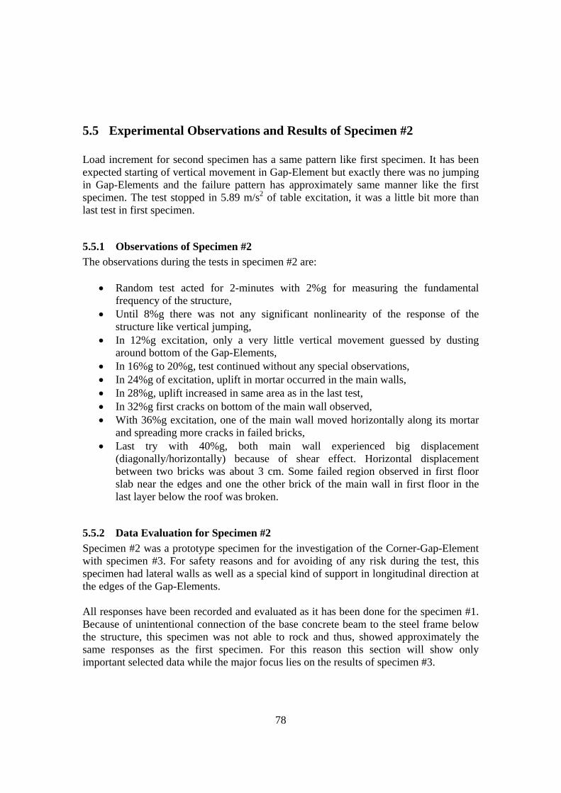
78

5.5 Experimental Observations and Results of Specimen #2 Load increment for second specimen has a same pattern like first specimen. It has been expected starting of vertical movement in Gap-Element but exactly there was no jumping in Gap-Elements and the failure pattern has approximately same manner like the first specimen. The test stopped in 5.89 m/s2 of table excitation, it was a little bit more than last test in first specimen.

5.5.1 Observations of Specimen #2 The observations during the tests in specimen #2 are:

• Random test acted for 2-minutes with 2%g for measuring the fundamental frequency of the structure,

• Until 8%g there was not any significant nonlinearity of the response of the structure like vertical jumping,

• In 12%g excitation, only a very little vertical movement guessed by dusting around bottom of the Gap-Elements,

• In 16%g to 20%g, test continued without any special observations, • In 24%g of excitation, uplift in mortar occurred in the main walls, • In 28%g, uplift increased in same area as in the last test, • In 32%g first cracks on bottom of the main wall observed, • With 36%g excitation, one of the main wall moved horizontally along its mortar

and spreading more cracks in failed bricks, • Last try with 40%g, both main wall experienced big displacement

(diagonally/horizontally) because of shear effect. Horizontal displacement between two bricks was about 3 cm. Some failed region observed in first floor slab near the edges and one the other brick of the main wall in first floor in the last layer below the roof was broken.

5.5.2 Data Evaluation for Specimen #2 Specimen #2 was a prototype specimen for the investigation of the Corner-Gap-Element with specimen #3. For safety reasons and for avoiding of any risk during the test, this specimen had lateral walls as well as a special kind of support in longitudinal direction at the edges of the Gap-Elements. All responses have been recorded and evaluated as it has been done for the specimen #1. Because of unintentional connection of the base concrete beam to the steel frame below the structure, this specimen was not able to rock and thus, showed approximately the same responses as the first specimen. For this reason this section will show only important selected data while the major focus lies on the results of specimen #3.

79

Specimen #2

6.60

6.65

6.70

6.75

6.80

6.85

6.90

6.95

0.5 1 1.5 2 2.5 3 3.5 4 4.5 5Maximum Table Excitation [ m / s ² ]

Fund

amen

tal F

requ

ency

of

the

Stru

ctur

e [ H

z ]

Figure 5-15 Fundamental frequency reduction (random-test result), specimen #2

Figure 5-15 shows fundamental frequency reduction, except of the last test (failure in structure) there is practically no reduction. This means that the structure did not experience any kind of cracks or failures until the last test. Figure 5-16 shows the overturning moment and maximum roof displacement. It is noticeable the different behavior of this specimen in compared with specimen #1, although their structure and loading were similar.

80

Specimen #2

50

100

150

200

250

300

0 5 10 15 20 25 30 35 40 45Maximum Roof Displacement [ mm ]

Max

imum

Ove

rtur

ning

Mom

ent [

kN

. m

]

Figure 5-16 Maximum overturning moment vs. maximum roof displacement,

specimen #2 Maximum roof responses are similar as for the first specimen, Figure 5-13.

Specimen #2

0

2

4

6

8

10

12

14

16

0 0.5 1 1.5 2 2.5 3 3.5 4 4.5 5 5.5 6Maximum Table Excitation [ m / s ² ]

Max

imum

Roo

f Res

pons

es [

m /

s ² ]

First Floor Response

Second floor Response

Figure 5-17 Maximum roof responses vs. maximum table excitation, specimen #2

81

5.6 Experimental Observations and Results of Specimen #3 Specimen number three built with following changes:

• Lower total weight compared to last specimens (because of removing the lateral walls),

• Changing the shear system in Gap-Element that described in Appendix - C, Figure C-10-b,

• Put new steel strip between Gap-Elements and first floor Appendix - C, Figure C-10-a.

Same marking the cracks was done for this specimen, but the number of the marked cracks was less than of specimen #2. In specimen #3 observations could satisfy the expected behavior of the Gap-Element. Structure could resist until 80%g (12.03 m/s2) excitation and finally second floor collapsed and the first floor with Gap-Elements was safe and ready to continue the test.

5.6.1 Observations of Specimen #3 Below brought all of the observations during the test:

• Random test like last specimens calculated 6.6 Hz for fundamental frequency, • 4%g till 10%g everything was same as last specimens, • In 12%g first vertical movement observed in Gap-Elements (the dust appeared

around the notches of Gap-Elements), • There were not any cracks until 12%g, • The test continued until 20%g with increasing vertical movement in rocky

motion, same uplift happened in same layer as last specimens, • Test continued until 24%g without any special effects, • In 28%g, last layer in main wall below first floor one brick cracked. In this test

one marker put between the first roof and the beam of steel frame in order to specify the contact between structure and safety frame. In case of any contact, the beam in steel frame could move in lower position, see Figure 5-18.

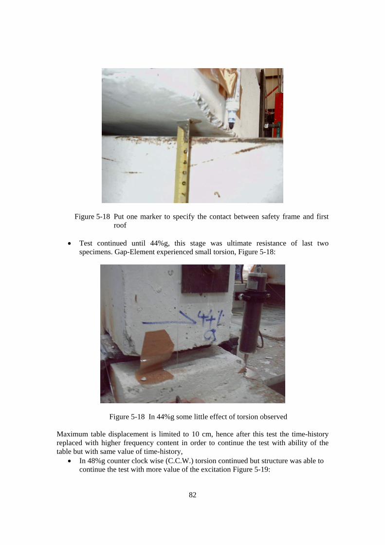
82

Figure 5-18 Put one marker to specify the contact between safety frame and first roof

• Test continued until 44%g, this stage was ultimate resistance of last two

specimens. Gap-Element experienced small torsion, Figure 5-18:

Figure 5-18 In 44%g some little effect of torsion observed Maximum table displacement is limited to 10 cm, hence after this test the time-history replaced with higher frequency content in order to continue the test with ability of the table but with same value of time-history,

• In 48%g counter clock wise (C.C.W.) torsion continued but structure was able to continue the test with more value of the excitation Figure 5-19:

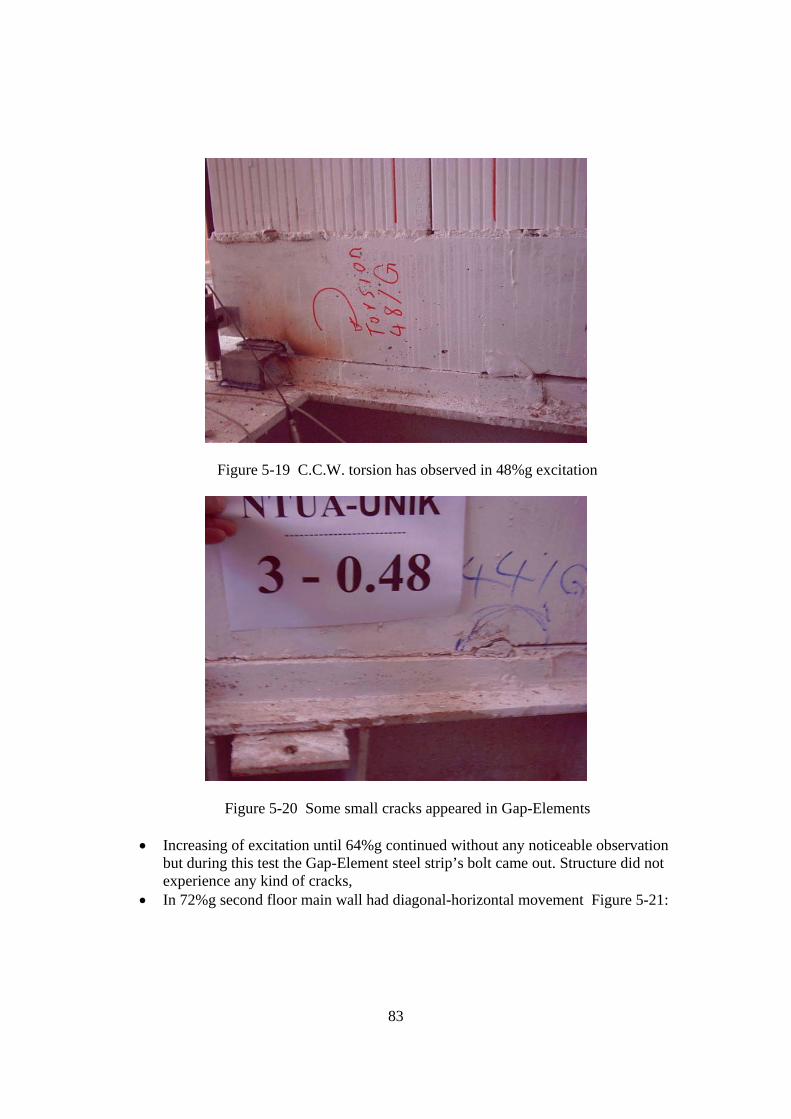
83

Figure 5-19 C.C.W. torsion has observed in 48%g excitation

Figure 5-20 Some small cracks appeared in Gap-Elements

• Increasing of excitation until 64%g continued without any noticeable observation but during this test the Gap-Element steel strip’s bolt came out. Structure did not experience any kind of cracks,

• In 72%g second floor main wall had diagonal-horizontal movement Figure 5-21:

84

Figure 5-21 Diagonal cracks in mortar occurred in 72%g excitation

• 80%g was the last try, the structure failed in the main wall in the second floor completely, whole main wall in second floor collapsed Figure 5-22 to Figure 5-25:

(a) (b)

Figure 5-22 Failure of second floor in 80%g excitation (12.03 m/s2)

85

Figure 5-23 Big horizontal movement in second floor main wall (12 cm)

Figure 5-24 Shear failure in first layer of second floor main wall in last try (80%g) In Figure 5-22-a torsion effect in second floor is cleared, parallel main wall in second floor did not have any big failure as it occurred in the opposite wall Figure 5-25:

86

(a) (b)

Figure 5-25 Second floor main wall without any big failure in last try (80%g)

5.6.2 Data Evaluation for Specimen #3 Specimen #3 had been made with Corner-Gap-Elements and it showed different behavior in comparison with the first specimen, as expected. For comparing the results, the figures in this section use the same ordering as for the first specimen but more details are included. Loading procedure was the same as for the first specimen. The increase of loads for the subsequent loading-step was equal, too. The first figure in this series shows the behavior of the structure during the test.

Specimen #3

0

2

4

6

8

10

12

14

16

0 1 2 3 4 5 6 7 8 9 10 11 12Maximum Table Excitation [ m / s ² ]

Max

imum

Roo

f Res

pons

es [

m /

s ² ]

First Floor Response

Second Floor Response

Figure 5-26 Maximum table excitation vs. maximum floor responses, specimen #3

87

Figure 5-26 depicts the responses of both roofs during the whole test series. The excitation rate increased to more than 12 m/s2. This rather high value documents the improvement of structure’s behavior by using the Gap-Element method. Secondly, it should be noted that the second floor response shows a parallel curve with X-axis approximately after 4 m/s2 excitation, although the first roof increased its response to big values up to 15 m/s2.

Specimen #3

0

10

20

30

40

50

60

70

80

0 10 20 30 40 50 60 70 80 90 100 110

Maximum Table Displacement [ mm ]

Max

imum

Roo

f Dis

plac

emen

ts [

mm

] First Floor Second floor

Figure 5-27 Maximum table displacement vs. maximum roofs displacement,

specimen #3 Maximum horizontal displacements of the roofs are shown in Figure 5-27. Both roofs were moving in parallel, but after changing the shaking-table excitation mode (because the maximum allowable horizontal movement of the table is 100 mm, the control signal had to be high pass filtered. For details, see Appendix -D), the roofs increased their displacement with bigger slope and finally the second floor collapsed with too much displacement because of the general roof rotation and brick’s failure. This graph consists of two separate parts; in the first part, the structure experienced the table displacement, meanwhile the second part of the graph starts with low value of table displacement. Finally in the second part, the shaking-table provoked the specimen to failure. Shear forces in roofs are one of the other result could give a good judgment to describe structure behavior. Figure 5-28 is about roof’s shear forces compared with roof’s displacement. This figure shows the first roof with big shear forces compared to the second roof.

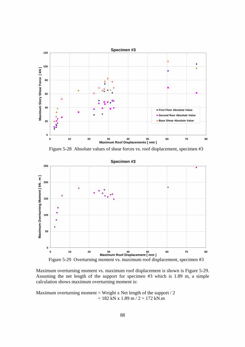
88

Specimen #3

0

50

100

150

200

250

0 10 20 30 40 50 60 70 80Maximum Roof Displacement [ mm ]

Max

imum

Ove

rtur

ning

Mom

ent [

kN

. m

]

Specimen #3

0

20

40

60

80

100

120

0 10 20 30 40 50 60 70 80Maximum Roof Displacements [ mm ]

Max

imum

Sto

ry S

hear

For

ce [

kN

]

First Floor Absolute Value

Second floor Absolute Value

Base Shear Absolute Value

Figure 5-28 Absolute values of shear forces vs. roof displacement, specimen #3

Figure 5-29 Overturning moment vs. maximum roof displacement, specimen #3 Maximum overturning moment vs. maximum roof displacement is shown is Figure 5-29. Assuming the net length of the support for specimen #3 which is 1.89 m, a simple calculation shows maximum overturning moment is: Maximum overturning moment = Weight x Net length of the support / 2 = 182 kN x 1.89 m / 2 = 172 kN.m

89

High value of overturning moment from last test in Figure 5-29 is related to the failure in the walls of second floor in last test and consequently recording high values of the acceleration in the roofs. For calculating the overturning moment all of the dynamic effects are included, as follows:

• The effect of dynamic vertical forces, • Rotational inertia.

Maximum base shear with maximum top displacement for specimen #3 are tabulated in Table 5-3 (see Figure 5-14 for detail). For calculating ductility or any other related parameters, it is assumed that the test 3-12 and further tests are entered to the ductile mode:

Table 5-3 Maximum base shear and related top displacement for tests in

specimen #3

Test Number Base Shear

Maximum [kN] Top Displacement Maximum [mm]

2 20.08 2.27 4 26.95 3.18 6 33.50 3.41 8 38.66 3.91

10 52.94 6.07 12 65.21 14.69 14 61.14 22.57 16 64.97 26.86 18 65.81 30.96 20 69.14 32.67 22 67.40 27.80 24 68.93 25.07 26 78.23 28.14 28 82.71 29.59 30 78.06 31.95 32 107.88 60.55 34 97.80 75.08

Figure 5-30 shows roofs rotation around the vertical axis. Rotation is low until the last test because no significant damage occurred until then. After the second storey lost its stiffness, it rotated around the vertical axis.

90

Specimen #3

0

10

20

30

40

50

60

0 10 20 30 40 50 60 70 80Maximum Roof Displacements [ mm ]

Max

imum

Lat

eral

Dis

plac

emen

ts o

f Roo

fs [

mm

]

First Floor

Second floor

Specimen #3

0

0.5

1

1.5

2

2.5

3

0 10 20 30 40 50 60 70 80Maximum Roof Displacements [ mm ]

Max

imum

Roo

f Rot

atio

ns [

Deg

] First Floor

Second floor

Figure 5-30 Roofs rotation vs. roof displacement, specimen #3

Figure 5-31 Roof lateral displacement vs. roof displacement, specimen #3 Lateral displacement is the subject of Figure 5-31. This figure is generated for evaluating jumping and rotation of the whole structure around the vertical axis. The slip-stopper in notches could control this special kind of rotation during the excitation.

91

Specimen #3

0

5

10

15

20

25

30

35

0 5 10 15 20 25 30 35 40 45 50 55 60 65 70 75 80

Maximum Roof Displacements [ mm ]

Max

imum

Ver

tical

Dis

plac

emen

ts o

f Roo

fs [

mm

]

First Floor (Relative to the Gap-Element)

Second floor (Relative to the first floor)

Total

Figure 5-32 Maximum vertical and horizontal displacement of the roofs, specimen

#3 Figure 5-32 shows maximum vertical displacement of the roofs vs. maximum horizontal roof displacement. Figure 5-32 clearly depicts that the first roof starts to jump in compatible path with second roof during the tests. The recorded movies from the tests confirmed these vertical movements (like a rocking motion of rigid block). Some higher values of vertical displacement of second roof in comparison with first roof are related to the mortar discontinuity in second storey (this case is observed during the tests).

Specimen #3

0

5

10

15

20

25

0 10 20 30 40 50 60 70 80Maximum Roof Displacements [ mm ]

Max

imum

Ver

tical

Gap

Dis

plac

emen

ts [

mm

]

Figure 5-33 Maximum Gap-Element vertical displacement vs. maximum horizontal

roofs displacement, specimen #3

92

The development of the fundamental frequency is shown in Figure 5-34. This figure represents a normal behavior of any structure after experiencing many earthquake loadings. Here the specimen had frequencies from 6.7 Hz (T=0.15 s) to 5.2 Hz (T=0.19 s).

Specimen #3

0

1

2

3

4

5

6

7

0 1 2 3 4 5 6 7 8 9 10 11 12 13Maximum Table Excitation [ m / s ² ]

Fund

amen

tal F

requ

ency

of

the

Stru

ctur

e [ H

z ]

Figure 5-34 Fundamental frequency reduction, specimen #3

Specimen #3

0

20

40

60

80

100

120

0 2 4 6 8 10 12 14Maximum Table Excitation [ m / s ² ]

Max

imum

Tab

le D

ispl

acem

ent [

mm

]

Figure 5-35 Maximum table displacement vs. maximum table excitation, specimen

#3

93

With test specimen #3, the table reached to its limitations. As explained in the table's specification, it had maximum allowable horizontal movement 10 cm. In order to be able to apply higher table accelerations, the controlling signal had to be modified by low pass filtering. Figure 5-35 shows details and in the Appendix - D, the modified table response spectrum is being discussed.

5.6.2.1 Result for Load Step 10 This documentation considers specimen #3, with maximum table excitation of 3.304 m/s2. Figure 5-36 shows the time-history of loading and its spectrum (F.F.T. Method). Maximum peak value of the table excitation is near second 4.

Figure 5-36 Table excitation and FFT-spectrum, load step 10

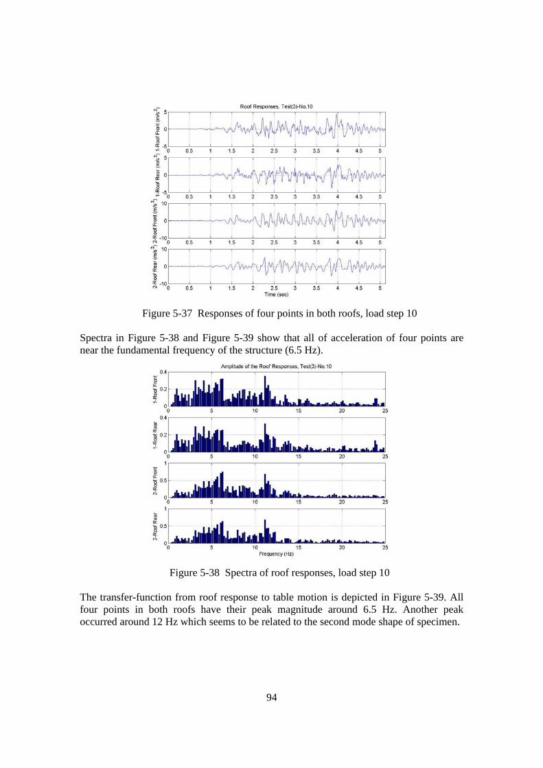
94

Figure 5-37 Responses of four points in both roofs, load step 10

Spectra in Figure 5-38 and Figure 5-39 show that all of acceleration of four points are near the fundamental frequency of the structure (6.5 Hz).

Figure 5-38 Spectra of roof responses, load step 10

The transfer-function from roof response to table motion is depicted in Figure 5-39. All four points in both roofs have their peak magnitude around 6.5 Hz. Another peak occurred around 12 Hz which seems to be related to the second mode shape of specimen.

95

Figure 5-39 Transfer-functions of four points, load step 10

The force-displacement graph is discussed in Figure 5-40. In this figure, the generated shear force in second roof vs. its horizontal displacement shows that the structure tried to enter in nonlinear behavior.

Specimen #3, Top Story Test (10)

-30

-20

-10

0

10

20

30

-5 -4 -3 -2 -1 0 1 2 3 4 5 6 7Displacement 2-Floor [ mm ]

Shea

r For

ce in

2-F

loor

[ kN

]

Figure 5-40 Second floor shear force vs. displacement, load step 10

Figure 5-41 has the same duty as Figure 5-40 but for roof number one.

96

Specimen #3, Test (10)

-60

-40

-20

0

20

40

60

-6 -4 -2 0 2 4 6 8Displacement 2-Floor [ mm ]

Bas

e Sh

ear [

kN

]

Figure 5-41 Base shear vs. displacement of the second floor, load step 10

Figure 5-42 shows a comparison of base acceleration and responses in the first roof of the structure.

Specimen #3, First Roof Responses Test (10)

-5

-4

-3

-2

-1

0

1

2

3

4

5

0 0.5 1 1.5 2 2.5 3 3.5 4 4.5 5Time [ s ]

Acc

eler

atio

n [ m

/ s

² ]

1-Roof Front1-Roof RearTable - Excitation

Figure 5-42 Responses of the first roof, load step 10

The data from the two accelerometers installed for recording lateral responses are given in Figure 5-43. The order of magnitude is about 50 % of the longitudinal excitation.

97

Specimen #3, First Roof Lateral Response Test(10)

-3

-2

-1

0

1

2

3

4

0 0.5 1 1.5 2 2.5 3 3.5 4 4.5 5Time [ s ]

Acc

eler

atio

n [ m

/ s

² ]

1-Roof Left1-Roof RightTable Excitation

Figure 5-43 Lateral accelerations of the first storey, load step 10

Figure 5-46 shows the same parameters as the last two figures but for the second roof.

Specimen #3, Second Roof Responses Test (10)

-8

-6

-4

-2

0

2

4

6

8

0 0.5 1 1.5 2 2.5 3 3.5 4 4.5 5Time [ s ]

Acc

eler

atio

n [ m

/ s

² ]

2-Roof Front2-Roof RearTable - Excitation

Figure 5-44 Responses of the second roof, load step 10

Lateral responses from the top storey are expressed by Figure 5-45. This figure shows that the second roof lateral nodes had acceleration values similar to the table excitation; a fact which has to be considered in theoretical modeling.

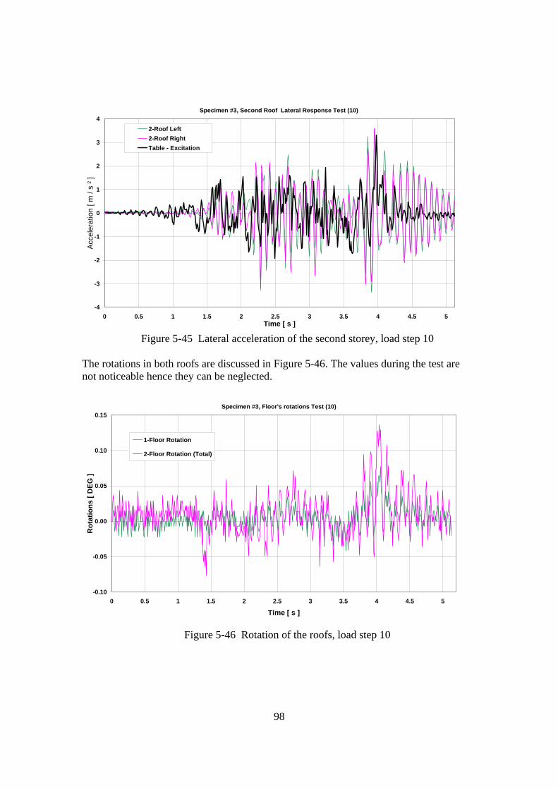
98

Specimen #3, Second Roof Lateral Response Test (10)

-4

-3

-2

-1

0

1

2

3

4

0 0.5 1 1.5 2 2.5 3 3.5 4 4.5 5Time [ s ]

Acc

eler

atio

n [ m

/ s

² ]

2-Roof Left2-Roof RightTable - Excitation

Figure 5-45 Lateral acceleration of the second storey, load step 10

The rotations in both roofs are discussed in Figure 5-46. The values during the test are not noticeable hence they can be neglected.

Specimen #3, Floor's rotations Test (10)

-0.10

-0.05

0.00

0.05

0.10

0.15

0 0.5 1 1.5 2 2.5 3 3.5 4 4.5 5

Time [ s ]

Rot

atio

ns [

DEG

]

1-Floor Rotation

2-Floor Rotation (Total)

Figure 5-46 Rotation of the roofs, load step 10

99

Figure 5-47 Roof’s rotations in frequency domain, load step 10

Figure 5-47 and Figure 5-48 show the spectra for the rotations of the roofs as well as the transfer-function in relation to the table acceleration. The resonance of both roofs is around 1 Hz and thus, far away from the first fundamental frequency of the undamaged structure. The values, however, are still small so the rotation effect of the roofs can be neglected at this stage.

Figure 5-48 Transfer function of Roof’s rotations, load step 10

The average vertical displacement is compared with the average horizontal displacement for the nodes of first storey, Figure 5-49.

100

Specimen #3, First Story Test (10)

-5

-4

-3

-2

-1

0

1

2

3

4

5

-4 -3 -2 -1 0 1 2 3 4 5Horizontal Displacement of 1-Floor [ mm ]

Vert

ical

Dis

plac

emen

t of 1

-Flo

or [

mm

]

Point 1 Point 2

Point 3 Point 4

Figure 5-49 Vertical displacement vs. horizontal displacement of the first storey, load

step 10

Specimen #3, Second Story Test (10)

-5

-4

-3

-2

-1

0

1

2

3

4

5

-8 -6 -4 -2 0 2 4 6 8 10 12 14Total Horizontal Displacement [ mm ]

Vert

ical

Dis

plac

emen

t of 2

-Flo

or [

mm

]

Point 5 Point 6

Point 7 Point 8

Figure 5-50 Vertical displacement vs. horizontal displacement of the second storey,

load step 10

101

The Figure 5-50 and Figure 5-51 show that, only small vertical deformations have occurred in both storeys. Gap-Elements started to “jump” near the peak points of the forcing function (around second 4). Figure 5-51 shows some asymmetry occurs since only one Gap-Element shows significant “Jumping”.

Specimen #3 Test (10)

-1

-0.5

0

0.5

1

1.5

2

2.5

0 0.5 1 1.5 2 2.5 3 3.5 4 4.5 5Time [ s ]

Vert

ical

Dis

plac

emen

t of G

ap-E

lem

ent [

mm

] Front-LeftFront-RightRear-LeftRear-Right

Figure 5-51 Vertical displacement of Gap-Elements, load step 10

102

5.6.2.2 Result for Load Step 20 For this load step, the same sequence of figures is depicted in the following for a maximum table excitation 5.096 m/s2. Figure 5-52 depicts the table acceleration.

Figure 5-52 Table excitation and FFT-spectrum, load step 20

Figure 5-53 expresses responses of the roofs for this load step again.

Figure 5-53 Responses of four points in both roofs, load step 20

103

Comparing Figure 5-54 with 5-40 it becomes evident, that the dominating frequency range has shifted significantly towards lower frequencies.

Figure 5-54 Spectra of roof responses, load step 20

Figure 5-55 indicates the transfer function. Near 3 Hz and 10 Hz high values are shown. Resonance effects above 13 Hz can be neglected.

Figure 5-55 Transfer-function of four points, load step 20

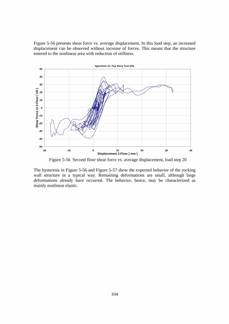
104

Figure 5-56 presents shear force vs. average displacement. In this load step, an increased displacement can be observed without increase of forces. This means that the structure entered to the nonlinear area with reduction of stiffness.

Specimen #3, Top Story Test (20)

-50

-40

-30

-20

-10

0

10

20

30

40

50

-20 -10 0 10 20 30 40Displacement 2-Floor [ mm ]

Shea

r For

ce in

2-F

loor

[ kN

]

Figure 5-56 Second floor shear force vs. average displacement, load step 20

The hysteresis in Figure 5-56 and Figure 5-57 show the expected behavior of the rocking wall structure in a typical way. Remaining deformations are small, although large deformations already have occurred. The behavior, hence, may be characterized as mainly nonlinear elastic.

105

Specimen #3, Test (20)

-80

-60

-40

-20

0

20

40

60

80

-20 -10 0 10 20 30 40Displacement 2-Floor [ mm ]

Bas

e Sh

ear [

kN

]

Figure 5-57 Base shear vs. displacement of the second floor, load step 20

Specimen #3, First Roof Responses Test (20)

-10

-8

-6

-4

-2

0

2

4

6

8

0 0.5 1 1.5 2 2.5 3 3.5 4 4.5 5Time [ s ]

Acc

eler

atio

n [ m

/ s

² ]

1-Roof Front1-Roof RearTable - Excitation

Figure 5-58 Responses of the first roof, load step 20

Lateral acceleration response in the first roof confirms the rotational movement in the roof. In Figure 5-59 it can be seen that the lateral accelerations show rather high values.

106

For the first roof, as during the previous load step response, approximately 50% of table excitation could be recorded.

Specimen #3, First Roof Lateral Response Test (20)

-5

-4

-3

-2

-1

0

1

2

3

4

5

6

0 0.5 1 1.5 2 2.5 3 3.5 4 4.5 5Time [ s ]

Acc

eler

atio

n [ m

/ s

² ]

1-Roof Left1-Roof RightTable-Excitation

Figure 5-59 Lateral acceleration of first storey, load step 20

Second roof responses are specified in Figure 5-60.

Specimen #3, Second Roof Responses Test (20)

-8

-6

-4

-2

0

2

4

6

8

0 0.5 1 1.5 2 2.5 3 3.5 4 4.5 5Time [ s ]

Acc

eler

atio

n [ m

/ s

² ]

2-Roof Front2-Roof RearTable - Excitation

Figure 5-60 Responses of second roof, load step 20

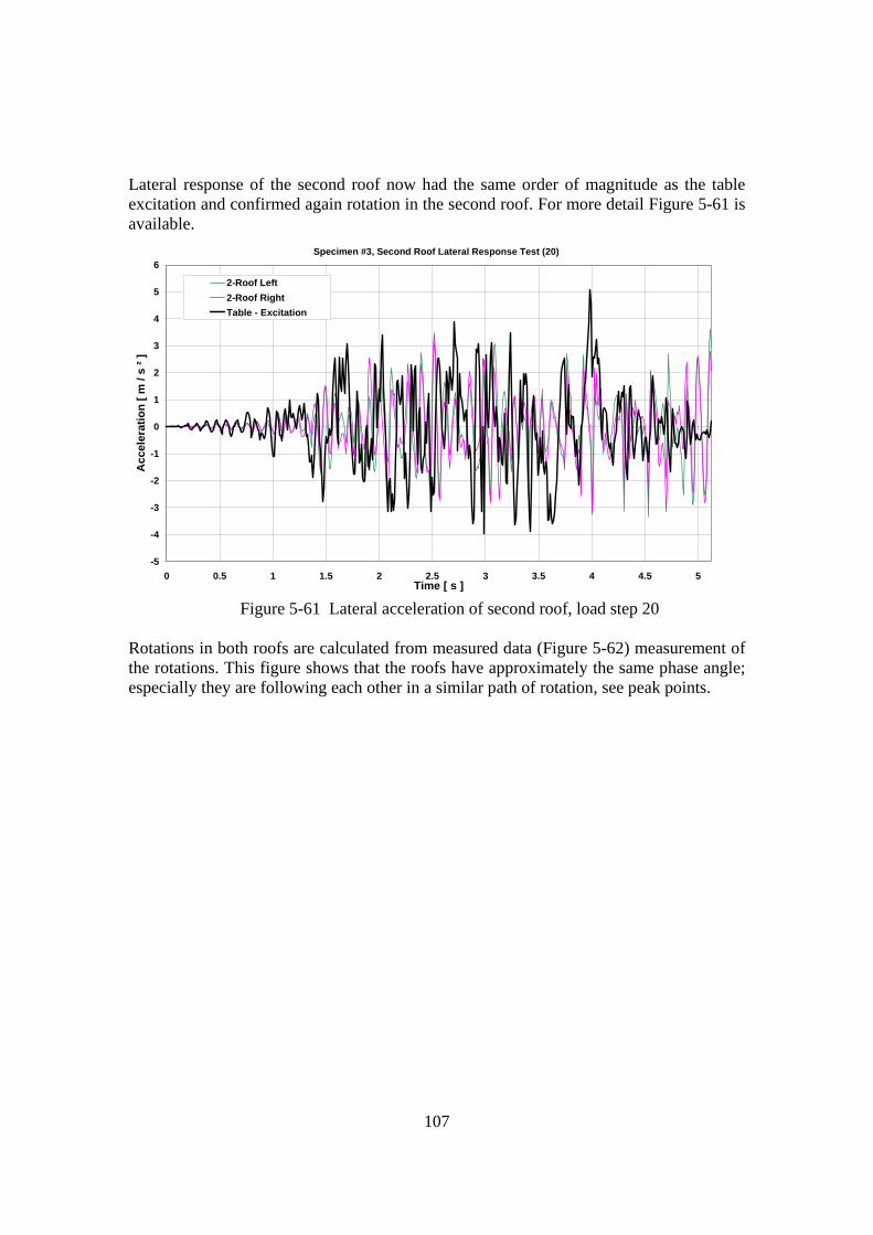
107

Lateral response of the second roof now had the same order of magnitude as the table excitation and confirmed again rotation in the second roof. For more detail Figure 5-61 is available.

Specimen #3, Second Roof Lateral Response Test (20)

-5

-4

-3

-2

-1

0

1

2

3

4

5

6

0 0.5 1 1.5 2 2.5 3 3.5 4 4.5 5Time [ s ]

Acc

eler

atio

n [ m

/ s

² ]

2-Roof Left2-Roof RightTable - Excitation

Figure 5-61 Lateral acceleration of second roof, load step 20

Rotations in both roofs are calculated from measured data (Figure 5-62) measurement of the rotations. This figure shows that the roofs have approximately the same phase angle; especially they are following each other in a similar path of rotation, see peak points.

108

Specimen #3, Floor's rotations Test (20)

-0.15

-0.10

-0.05

0.00

0.05

0.10

0.15

0.20

0.25

0 0.5 1 1.5 2 2.5 3 3.5 4 4.5 5

Time [ s ]

Rot

atio

ns [

DEG

]

1-Floor Rotation

2-Floor Rotation (Total)

Figure 5-62 Roof’s rotations, load step 20

In Figure 5-47 is shown that most of the resonance frequency becomes lower and Figure 5-63 shows this effect for load step 20 again.

Figure 5-63 Roof’s rotations in frequency domain, load step 20

Transfer-function for rotations are calculated and depicted in Figure 5-64.

109

Figure 5-64 Transfer-function Roof’s rotations, load step 20

Figure 5-65 shows vertical displacement of the first floor vs. average horizontal displacement due to the effect of rocking. The shape of the curves corresponds well with the expected behavior.

Specimen #3, First Story Test (20)

-4

-2

0

2

4

6

8

10

12

-10 -7.5 -5 -2.5 0 2.5 5 7.5 10 12.5 15 17.5 20Horizontal Displacement of 1-Floor [ mm ]

Vert

ical

Dis

plac

emen

t of 1

-Flo

or [

mm

]

Point 1

Point 2

Point 3

Point 4

Figure 5-65 Vertical displacement vs. horizontal displacement of the first storey, load

step 20

110

Figure 5-66 has same target as Figure 5-65 but for the second roof. Specimen #3, Second Story Test (20)

-4

-2

0

2

4

6

8

10

12

-30 -20 -10 0 10 20 30 40 50 60Total Horizontal Displacement [ mm ]

Vert

ical

Dis

plac

emen

t of 2

-Flo

or [

mm

]

Point 5Point 6Point 7Point 8

Figure 5-66 Average vertical displacement vs. average horizontal displacement of the

second storey, load step 20 This test shows all four edges of Gap-Elements in the two longitudinal walls started to jump according to the rocking motion, Figure 5-67:

Specimen #3 Test (20)

-4

-2

0

2

4

6

8

10

12

14

0 0.5 1 1.5 2 2.5 3 3.5 4 4.5 5Time [ s ]

Vert

ical

Dis

plac

emen

t of G

ap-E

lem

ent [

mm

]

Front-Left

Front-Right

Rear-Left

Rear-Right

Figure 5-67 Vertical displacement of Gap-Element, load step 20

111

5.6.2.3 Result for Load Step 30 This load step shows figures of the test before the last one in specimen #3, with maximum table excitation 9.093 m/s2. The test data of the following load step are difficult to interpret, because the specimen had severe damage of the main walls. Hence, this load step (#30) has been selected for this documentation. Figure 5-68 shows the time-history of loading and spectrum for this load step.

Figure 5-68 Table excitation and FFT-spectrum, load step 30

Figure 5-69 shows responses in the roofs, but here more data had been recorded up to 8.12 seconds. Free vibrations are shown after finishing the table excitation (after 5.12 s).

Figure 5-69 Responses of four points in both roofs, load step 30

112

Figure 5-70 explains that above 15 Hz, the response of the second roof had a lower magnitude in comparison with the first roof. One of the reasons obviously is related to the nonlinear behavior of the structure. The structure avoids to have any response in high frequencies.

Figure 5-70 Spectra of roof responses, load step 30

The first roof acted like a shaking-table for the second roof. When the test finished (because of the failure of the second storey), the first storey was totally able to continue the test. The transfer-functions confirmed this claim too, Figure 5-71:

Figure 5-71 Transfer-function of four points, load step 30

113

The next figure shows the nonlinear behavior of the second storey for specimen #3. During this test some small cracks occurred.

Specimen #3, Top Story Test (30)

-60

-40

-20

0

20

40

60

-40 -30 -20 -10 0 10 20 30 40Displacement 2-Floor [ mm ]

Shea

r For

ce in

2-F

loor

[ kN

]

Figure 5-72 Second floor shear force vs. displacement, load step 30

Figure 5-72 clearly shows the nonlinear behavior of the specimen. Instead of a straight plateau of horizontal shear forces, some deviations occur. This can be attributed to higher mode responses and the effect of vertical inertia forces enabling higher overturning moments and, thus, shear forces. Figure 5-73 depicts the base shear vs. second floor horizontal displacement. Big values of horizontal displacement without significant increase of base shear demonstrate the effectiveness of the force limitation that is provided by Gap-Elements.

114

Specimen #3, Test (30)

-80

-60

-40

-20

0

20

40

60

80

100

-40 -30 -20 -10 0 10 20 30 40Displacement 2-Floor [ mm ]

Bas

e Sh

ear [

kN

]

Figure 5-73 Base shear vs. displacement of the second floor, load step 30

Main wall accelerometers recorded responses of the structure for the first floor. Figure 5-74 shows these data. These nodes did not report responses with an amount bigger than their source.

Specimen #3, First Roof Responses Test (30)

-10

-5

0

5

10

0 1 2 3 4 5 6 7 8Time [ s ]

Acc

eler

atio

n [ m

/ s

² ]

1-Roof Front1-Roof RearTable - Excitation

Figure 5-74 Responses of first roof, load step 30

115

Lateral responses of the first floor are shown in the Figure 5-75. In this load step same order of magnitude (50% of longitudinal excitation) is obtained and it is like the previous load steps 10 and 20 (Figure 5-45and Figure 5-59).

Specimen #3, First Roof Lateral Response Test (30)

-10

-5

0

5

10

0 1 2 3 4 5 6 7 8Time [ s ]

Acc

eler

atio

n [ m

/ s

² ]

1-Roof Left1-Roof RightTable-Excitation

Figure 5-75 Lateral acceleration of the first storey, load step 30

Specimen #3, Second Roof Responses Test (30)

-10

-5

0

5

10

0 1 2 3 4 5 6 7 8

Time [ s ]

Acc

eler

atio

n [ m

/ s

² ]

2-Roof Front2-Roof RearTable - Excitation

Figure 5-76 Responses of second roof, load step 30

116

Figure 5-77 shows that lateral responses in the second roof are close to those of the main direction of vibrating. Rotational effects are not considerable, as it is discussed before and confirmed by Figure 5-80.

Specimen #3, Second Roof Lateral Response Test (30)

-10

-8

-6

-4

-2

0

2

4

6

8

10

0 1 2 3 4 5 6 7 8Time [ s ]

Acc

eler

atio

n [ m

/ s

² ]

2-Roof Left2-Roof RightTable - Excitation

Figure 5-77 Lateral acceleration of the second storey, load step 30

For the remaining values of rotations in Figure 5-80 two reasons are conceivable:

1. The whole structure really rotated around vertical axis, e.g. due to rotational sliding on the foundation,

2. An error of the instrument has occurred in this test. For the next tests, however, everything was calibrated again.

117

Specimen #3, Floor's Rrotations Test (30)

-0.2

-0.1

0

0.1

0.2

0.3

0.4

0.5

0.6

0 1 2 3 4 5 6 7 8Time [ s ]

Rot

atio

ns [

DEG

]

First Floor Rotation

Second Floor Rotation(Total)

Figure 5-80 Roofs’ rotations, load step 30

Figure 5-81 Roof rotations in frequency domain, load step 30

The transfer-function is shown in Figure 5-82. This figure shows the rotational resonance has shifted to low frequencies.

118

Figure 5-82 Transfer-function of the roofs rotation, load step 30

Figure 5-83 shows the average vertical displacement in the first floor vs. average horizontal displacement. The maximum average vertical displacement in this load step is two times bigger than in the previous load step in the first floor. Negative values are due to rocking from which the notches in Corner-Gap-Elements are compressed.

Specimen #3, First Story Test (30)

-6

-4

-2

0

2

4

6

8

10

12

-17.5 -15 -12.5 -10 -7.5 -5 -2.5 0 2.5 5 7.5 10 12.5 15 17.5 20 22.5Horizontal Displacement of 1-Floor [ mm ]

Vert

ical

Dis

plac

emen

t of 1

-Flo

or [

mm

]

Point 1

Point 2

Point 3

Point 4

Figure 5-83 Vertical displacement vs. horizontal displacement of the first

storey, load step 30

119

Specimen #3, Second Story Test (30)

-5

-2.5

0

2.5

5

7.5

10

12.5

15

-50 -40 -30 -20 -10 0 10 20 30 40 50 60Total Horizontal Displacement [ mm ]

Vert

ical

Dis

plac

emen

t of 2

-Flo

or [

mm

]

Point 5 Point 6

Point 7 Point 8

Figure 5-84 Vertical displacement vs. horizontal displacement of the second

storey, load step 30 All of the four nodes in two Gap-Elements worked very well with response responding to the loading, Figure 5-85 shows details. Peak values are near 12 mm. It is remarkable that the structure did not suffer from those high values of vertical jumping and behaved stable until the end of the loading sequence.

Specimen #3, Test (30)

-2

0

2

4

6

8

10

12

0 0.5 1 1.5 2 2.5 3 3.5 4 4.5 5 5.5 6 6.5 7 7.5 8Time [ s ]

Vert

ical

Dis

plac

emen

t of G

ap-E

lem

ent [

mm

]

Front-Left

Front-Right

Rear-Left

Rear-Right

Figure 5-85 Vertical displacement of Gap-Element, load step 30

120

Figure 5-86 shows a significant hysteresis unlike for previous load steps. This indicates considerable damage in the second floor.

Specimen #3,TEST (30)

-2

0

2

4

6

8

10

12

-30 -20 -10 0 10 20 30 40 Horizontal Displacement of 2-Roof [ mm ]

Vert

ical

Dis

plac

emen

t of G

ap-E

lem

ent [

mm

]

Left Front

Right Front

Figure 5-86 Vertical Gap-Element displacement vs. horizontal roof

displacement, load step 30

121

6 COMPARISON OF ANALYTICAL CALCULATION WITH EXPERIMENTAL TESTS

6.1 Introduction This chapter evaluates the results of experimental research. Although as it is explained before the behavior of the Gap-Element was acceptable and it could satisfy the aimed target but the focus of this chapter is to investigate about the ability of Gap-Element to carry seismic loads more than two times bigger than the ability of an identical specimen without Gap-Element.

6.2 Comparison of Experimental Results with Capacity Spectrum Approach

A capacity curve (force-displacement) criteria is a modern method for explaining the responses of structures under seismic load. Calculations in the present section follow the method that is presented by Bachmann / Lang [38], [39]. Capacity curves are generally produced for first mode shape. This implies that the load distribution over the height of the building should comply with the first mode shape. The method is based on the elasto-plastic behavior of structures. The following assumptions are considered for analysis:

• Walls only carry shear forces along their strong axes; the shear force carrying capacity along the weaker axis is neglected,

• Floor diaphragms are assumed as totally rigid in their plane; as a consequence of this assumption equal displacement of the walls at the floor levels giving permission for superimposing the capacity curves of all the walls together:

( ) ( )jbj

V VΔ = Δ∑ (6.2.1)

j is the wall index, j=1,…, n and n is the total number of the bearing walls in one direction, • By attention to the symmetric geometry and loading (static and dynamic) the

torsion effect is neglected, • The interaction between walls and spandrels makes coupling effect. Due to the

concrete roof in the specimens and the walls without any windows; this effect is leading to a very low value (for complete reference see [38], [39]),

• It is assumed that the most critical section which determines the capacity of the structure is at the ground floor; hence the capacity of the wall on the first floor is considered as the capacity of the structure,

122

The capacity curve is identified by three parameters, the shear capacity of the wall mV , the nominal yield displacement at the top of the wall yΔ , and the nominal ultimate

displacement at the top the wall uΔ . These parameters are depending on the wall material, geometry of the structure and acting vertical loads. The following five short descriptions give calculation details for the capacity curve of the wall: I- Geometry and material of the walls and the structure In this stage the below parameters have to be defined:

• Total height of the building: totH , • Storey height: sth , • Compression strength orthogonal to the mortar bed: mxf , • Compression strength parallel to the mortar bed: 0.3my mxf f≥ , • Angle of internal friction: ( )tan φ , • Modulus of elasticity of masonry: mE , • Shear modulus of masonry: mG , • Stiffness reduction factor: 0/effk k .

II- Identification of structural walls In this step, the geometry of the walls is specified:

• Length of the wall: Wl , • Thickness of the wall: t , • Height of the pier: ph , • Effective moment inertia of the wall: effI , • Effective cross section of the wall: effA .

III- Normal forces calculation This step specifies the normal force acted on the walls at the ground level, due to the symmetric specimens in this research the total vertical load can apply on two walls as the one wall with double thickness or dividing the total normal load in two equal parts:

• Normal force acting on the walls at ground level: N The capacity curve calculation is based on the static force, but the presented calculations in this research have to consider dynamic forces. The effects of vertical dynamic forces have to include on the calculations of the normal forces. As it explained before the vertical accelerations did not record by shaking table’s computer, consequently the vertical accelerations are generated by theoretical methods. For obtaining the vertical accelerations there are two possibilities: first generating them from vertical displacement

123

(F.F.T. method, 5) or second, finding them out from FEM modeling. For solving this problem the first method was considered and the answers were acceptable, because the final calculations about the overturning moment or the shear criteria or other engineering aspects were compatible with those generated data. The effect of vertical dynamic force is considered as an extra force over the normal force according to the values of vertical accelerations. These values are considered only for the tests with noticeable vertical accelerations, for example for specimen #1, the normal force is 20% increased only for the calculations in the last three tests and for specimen #3 that coefficient was 50% only for half tests; see Table 6-1 for detail. IV- Capacity curves of the walls The calculation of the capacity curve of the walls follows below procedures:

• Height of the zero moment: 0h , • Maximum admissible shear force that does violate neither the stress nor the

sliding criterion is:

20

tan

(tan ) 2 tanmy w

mmy

f l t NV

N N f t h

φ

φ φ

⋅ ⋅ ⋅ ⋅=

+ ⋅ + ⋅ ⋅ ⋅ ⋅ (6.2.2)

• The yield displacement at the top of the wall has to be determined with below

equation:

0(3 )( )

6p p

y m toteff eff

h h hV H

EI GAκ⋅ −

Δ = ⋅ ⋅ +⋅

(6.2.3)

κ is the form factor that depends on the particular shape of the cross section, for rectangular cross section (our case) κ = 6/5,

• The ultimate displacement at the top of the wall can be estimated by the following equations:

nw

Nt l

σ =⋅

(6.2.4)

The ductility of the pier is determined as the normal stress acting on the pier; hence, these values give the maximum admissible drift of the wall with:

0.8 0.25u nδ σ= − ⋅ (6.2.5) Now the ductility of the pier is defined by:

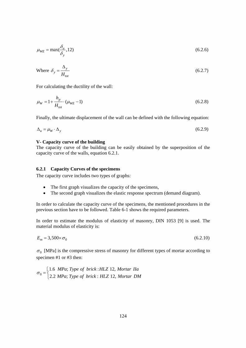
124

max( ,12)uWE

y

δμδ

= (6.2.6)

Where yy

totHδ

Δ= (6.2.7)

For calculating the ductility of the wall:

1 ( 1)pW WE

tot

hH

μ μ= + ⋅ − (6.2.8)

Finally, the ultimate displacement of the wall can be defined with the following equation:

u W yμΔ = ⋅Δ (6.2.9) V- Capacity curve of the building The capacity curve of the building can be easily obtained by the superposition of the capacity curve of the walls, equation 6.2.1.

6.2.1 Capacity Curves of the specimens The capacity curve includes two types of graphs:

• The first graph visualizes the capacity of the specimens, • The second graph visualizes the elastic response spectrum (demand diagram).

In order to calculate the capacity curve of the specimens, the mentioned procedures in the previous section have to be followed. Table 6-1 shows the required parameters. In order to estimate the modulus of elasticity of masonry, DIN 1053 [9] is used. The material modulus of elasticity is:

03,500mE σ= × (6.2.10)

0σ [MPa] is the compressive stress of masonry for different types of mortar according to specimen #1 or #3 then:

01.6 ; : 12,2.2 ; : 12,

MPa Type of brick HLZ Mortar IIaMPa Type of brick HLZ Mortar DM

σ⎧

= ⎨⎩

125

Table 6-1 Specimen specification

Specification

Specimen #1

Specimen #3

Total height of the building: totH [m] 4.40 4.26 Storey height: sth [m] 2.04 1.98 Comp. strength orthogonal to the mortar bed:

mxf [MPa] 1.60 x 2.67=4,27 2.20 x 2.67=5,87

Comp. strength parallel to the mortar bed: myf [MPa] ( 0.3my mxf f= ⋅ )

0.48 x 2.67=1,28 0.66 x 2.67=1,76

Angle of internal friction: tan( )φ 0.80 0.80 Modulus of elasticity of masonry: mE [MPa] 5600 7700 Shear modulus of masonry: mG [MPa] 1680 2310 Stiffness reduction factor: 0/effk k 0.50 0.50

Length of the wall: Wl [m] 2.23 2.23 / 1.90 Thickness of the wall: t [m] 0.35 0.35 Height of the pier: ph [m] 2.04 1.98 Effective moment of inertia of the wall:

effI [m4] 0.323 0.323 / 0.200

Effective cross section of the wall: effA [m2] 0.78 0.78 / 0.66 Normal force acting on walls at the ground level: N [kN]

192.36 182.40

Coefficient for increasing the normal force that caused by vertical acceleration

20% 50%

As it is explained before the capacity curve needs the shear force, yielding and ultimate displacement of top of the walls. Table 6-2 shows the calculated parameters by using the equations 6.2.1 until 6.2.9.

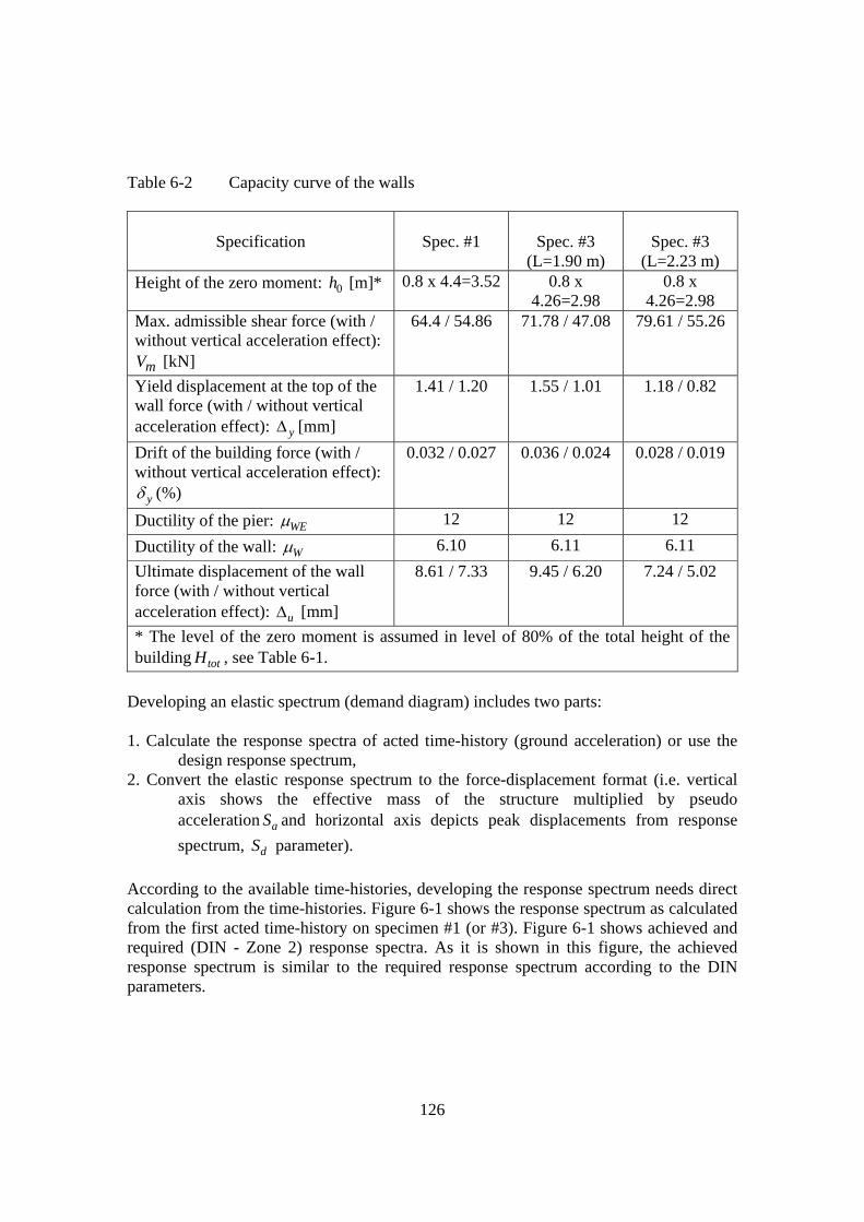
126

Table 6-2 Capacity curve of the walls

Specification

Spec. #1

Spec. #3

(L=1.90 m)

Spec. #3

(L=2.23 m) Height of the zero moment: 0h [m]* 0.8 x 4.4=3.52 0.8 x

4.26=2.98 0.8 x

4.26=2.98 Max. admissible shear force (with / without vertical acceleration effect):

mV [kN]

64.4 / 54.86 71.78 / 47.08 79.61 / 55.26

Yield displacement at the top of the wall force (with / without vertical acceleration effect): yΔ [mm]

1.41 / 1.20 1.55 / 1.01 1.18 / 0.82

Drift of the building force (with / without vertical acceleration effect):

yδ (%)

0.032 / 0.027 0.036 / 0.024 0.028 / 0.019

Ductility of the pier: WEμ 12 12 12 Ductility of the wall: Wμ 6.10 6.11 6.11 Ultimate displacement of the wall force (with / without vertical acceleration effect): uΔ [mm]

8.61 / 7.33 9.45 / 6.20 7.24 / 5.02

* The level of the zero moment is assumed in level of 80% of the total height of the building totH , see Table 6-1.

Developing an elastic spectrum (demand diagram) includes two parts: 1. Calculate the response spectra of acted time-history (ground acceleration) or use the

design response spectrum, 2. Convert the elastic response spectrum to the force-displacement format (i.e. vertical

axis shows the effective mass of the structure multiplied by pseudo acceleration aS and horizontal axis depicts peak displacements from response spectrum, dS parameter).

According to the available time-histories, developing the response spectrum needs direct calculation from the time-histories. Figure 6-1 shows the response spectrum as calculated from the first acted time-history on specimen #1 (or #3). Figure 6-1 shows achieved and required (DIN - Zone 2) response spectra. As it is shown in this figure, the achieved response spectrum is similar to the required response spectrum according to the DIN parameters.

127

Response Spectrum

0

0.2

0.4

0.6

0.8

1

1.2

1.4

1.6

1.8

2

0 0.25 0.5 0.75 1 1.25 1.5 1.75 2 2.25 2.5 2.75 3Period [s]

Acc

eler

atio

n [m

/s²]

DIN - Zone 2

Shaking table test (1- 2) 4%g, P.T.A. 0.599 m/s²

Figure 6-1 Comparison between required response spectrum (DIN - Zone 2) and

achieved response spectrum (calculated from time-history generated for test 1-2)

In the following, the mentioned procedures are calculated for both specimens (specimen #1 and specimen #3):

6.2.1.1 Capacity Diagrams for Specimen #1 Every individual test of specimens implemented by one time-history (see Figure 5-2) with different peak values, see Table 5-1. The response spectra for those time histories of specimen #1 are shown in Figure 6-2. It is noteworthy to express; these graphs are generated with recorded the real accelerations of shaking table, see section 5.3 for detail.

128

Response Spectra of the Building (Specimen #1)

0

2

4

6

8

10

12

14

0.0 0.3 0.6 0.9 1.2 1.5 1.8 2.1 2.4 2.7 3.0

Period [ s ]

Acc

eler

atio

n [ m

/s² ]

Test 1-2Test 1-4Test 1-6Test 1-8Test 1-10Test 1-12Test 1-14Test 1-16Test 1-18Test 1-20Test 1-22

Figure 6-2 Response spectra for achieved tests on specimen #1; based on the

recorded accelerations by shaking table (period domain) Figure 6-2 is repeated again with frequency domain in Figure 6-3.

Response Spectra of the Building (Specimen #1)

0

2

4

6

8

10

12

14

0 10 20 30 40 50 60 70 80 90 100

Frequency [Hz]

Acc

eler

atio

n [m

/s²]

Test 1-2Test 1-4Test 1-6Test 1-8Test 1-10Test 1-12Test 1-14Test 1-16Test 1-18Test 1-20Test 1-22

Figure 6-3 Response spectra for achieved tests on specimen #1; based on the

recorded accelerations by shaking table (frequency domain) For generating the capacity design curve the procedures can be listed as below:

129

1. Developing the capacity curve diagram of the building (shear force vs. top

displacement), 2. Developing the elastic design spectrum (demand diagram), 3. Plot the demand diagram and capacity diagram of the building together in one graph, 4. Evaluate the behavior of the wall (or structure) under the acted load and its capacity

(performance) for carrying such loads. Before to generate any graphs it is needed to consider that the achieved test specimens are more than one Degree Of Freedom (D.O.F.) consequently in order to develop the demand diagram it is necessary to calculate equivalent Single Degree Of Freedom (S.D.O.F.) system. Equivalent SDOF system Specimen #1 (or #3) is Multi Degrees Of Freedom system (M.D.O.F.); hence, the procedure is needed to convert the M.D.O.F. to a S.D.O.F., because the effect of different positions of masses has direct influence in all static calculations. The following formulation based on classical modal analysis approach shows the converting procedures: 1. The equivalent mass is given as:

E i iM m φ= ⋅∑ (6.2.11) In which im is the concentrated mass and iφ is the first mode displacement at the i-th floor level normalized such that the first mode displacement at the top storey nφ =1. 2. The equivalent height is:

i i iE

i i

h mh

mφφ

⋅ ⋅=

⋅∑∑

(6.2.12)

At which ih is the height of the i-th floor level.

3. The modal participation factor:

2i i

i i

mm

φφ⋅

Γ =⋅

∑∑

(6.2.13)

4. Convert factor Q that represents the quantities in the MDOF system (base shear bV ,

top displacement Δ ) and EQ represents the quantities in the equivalent SDOF system:

EQ Q= Γ ⋅ (6.2.14)

130

Then Table 6-5 shows the required data for the conversion of M.D.O.F. to S.D.O.F. for specimen #1:

Table 6-3 Modal approach parameters for specimen #1

Storey Level 1 Level 2 Mass [to] 10.65 8.59

Height [m] 2.13 4.31 First mode distribution 0.5 1.0

Then by using equations 6.3.8 - 6.3.11 the required data are given as:

E i iM m φ= ⋅∑ = 13.92 to

i i iE

i i

h mh

mφφ

⋅ ⋅=

⋅∑∑

= 3.47 m

2i i

i i

mm

φφ⋅

Γ =⋅

∑∑

= 1.24

Figure 6-4 shows all demand diagrams during the tests of specimen #1. Figure 6-5 includes the calculated capacity curve of the structure to Figure 6-4 (the effect of vertical acceleration is depicted too, see Table 6-1). The capacity of the structure in this figure clearly shows that the structure cannot carry those seismic loads, but in the experimental tests on the shaking table the responses of the structure were different, see further figures.

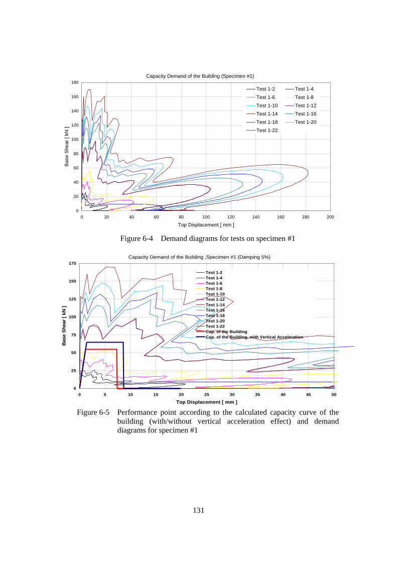
131

Capacity Demand of the Building (Specimen #1)

0

20

40

60

80

100

120

140

160

180

0 20 40 60 80 100 120 140 160 180 200

Top Displacement [ mm ]

Bas

e S

hear

[ kN

]

Test 1-2 Test 1-4Test 1-6 Test 1-8Test 1-10 Test 1-12Test 1-14 Test 1-16Test 1-18 Test 1-20Test 1-22

Figure 6-4 Demand diagrams for tests on specimen #1

Capacity Demand of the Building ,Specimen #1 (Damping 5%)

0

25

50

75

100

125

150

175

0 5 10 15 20 25 30 35 40 45 50

Top Displacement [ mm ]

Bas

e Sh

ear [

kN

]

Test 1-2Test 1-4Test 1-6Test 1-8Test 1-10Test 1-12Test 1-14Test 1-16Test 1-18Test 1-20Test 1-22Cap. of the Building Cap. of the Building, with Vertical Acceleration

Figure 6-5 Performance point according to the calculated capacity curve of the

building (with/without vertical acceleration effect) and demand diagrams for specimen #1

132

Figure 6-6 shows the real values from the shaking table data processing; there is difference between the demanded values and calculated values (shear capacity) in Figure 6-5 and experimental results in Figure 6-6.

Capacity Demand of the Building (Specimen #1)

0

10

20

30

40

50

60

70

80

0 2 4 6 8 10 12 14 16 18 20 22 24 26 28 30Top Displacement [ mm ]

Bas

e Sh

ear [

kN

] Experimental ResultsCapacity of the BuildingCap. of the Building, with Ver. Acc.

Figure 6-6 Comparison between calculated capacity and experimental results,

specimen #1 The inconsistent values in Figure 6-6 between theoretical calculations and real values maybe caused by the listed reasons:

• The capacity curve criteria is established on the static load and it did not consider all of dynamic effects, for example any jumping of the structure during the tests and its effect on the mortar,

• As it is mentioned before the capacity curve does not consider any effect of higher mode shapes, thus the structure’s behavior was not modeled according to its reality,

• After a shear force of about 60 kN, the walls entered in a ductile region and they experienced big values of ductile displacement (more than 8.61 mm see Table 6-2). Ductility more than 10 mm was not expected of such a masonry building without any ductile design approach, but the real data from experimental tests approved this ability in the structure,

• The demand diagrams are calculated to the real values of the acted seismic loads, according to the observations, and the big amount of experienced ductility by the structure and the ability of such a masonry building to these values of ductility there is some mismatching in the results. The reason of this mismatching will be in jumping of the roofs because of vertical acceleration and overturning moment,

• During seismic tests with high excitation (after test 1-16, see Table 5-1), some noticeable vertical jumping in the roofs is possible (in the last test, reveal jumping

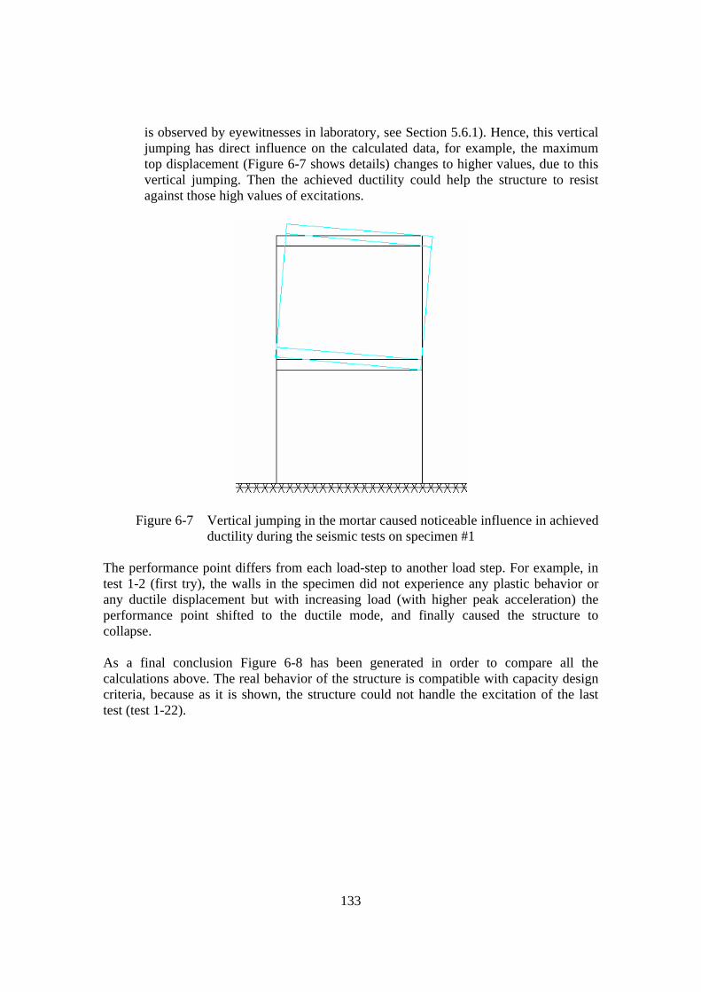
133

is observed by eyewitnesses in laboratory, see Section 5.6.1). Hence, this vertical jumping has direct influence on the calculated data, for example, the maximum top displacement (Figure 6-7 shows details) changes to higher values, due to this vertical jumping. Then the achieved ductility could help the structure to resist against those high values of excitations.

Figure 6-7 Vertical jumping in the mortar caused noticeable influence in achieved ductility during the seismic tests on specimen #1

The performance point differs from each load-step to another load step. For example, in test 1-2 (first try), the walls in the specimen did not experience any plastic behavior or any ductile displacement but with increasing load (with higher peak acceleration) the performance point shifted to the ductile mode, and finally caused the structure to collapse. As a final conclusion Figure 6-8 has been generated in order to compare all the calculations above. The real behavior of the structure is compatible with capacity design criteria, because as it is shown, the structure could not handle the excitation of the last test (test 1-22).

134

Capacity Demand of the Building ,Specimen #1 (Damping 5%)

0

25

50

75

100

125

150

175

0 5 10 15 20 25 30 35

Top Displacement [ mm ]

Bas

e Sh

ear [

kN

]

Test 1-2Test 1-4Test 1-6Test 1-8Test 1-10Test 1-12Test 1-14Test 1-16Test 1-18Test 1-20Test 1-22ExperimentalCap. of the Building Cap. of the Building, with Vertical Acceleration

Figure 6-8 Capacity criteria comparison between real values, expected and

calculated results, specimen #1 It is noteworthy to express that the recorded data for specimen #1 do not include damping ratios. Then it is assumed 5% for damping ratios, but for specimen #3 the damping ratios are recorded and for the last tests they are approximately 6 or 7 %. Consequently with the higher values of damping ratios the demand diagrams shift to left hand and the experimental results with calculated demand diagrams will meet each other on the right points.

6.2.1.2 Capacity Diagrams for Specimen #3 Same figures and procedures (like specimen #1) are shown in the following figures for specimen #3, but with some differences. The differences are related to the length of the notches in all of the calculations, because the length of the Gap-Element can be assumed in calculations with / without the notches. Figure 6-9 shows all the response spectra for acted time-histories for tests on specimen #3. Some scattered graphs are related to the complex behavior of the Gap-Element during the excitation, because the jumping of the Gap-Element could change the whole dynamic responses of the shaking table.

135

Response Spectra of the Building (Specimen #3), Damping Ratios Reported by Shaking Table

0

5

10

15

20

25

0.0 0.3 0.6 0.9 1.2 1.5 1.8 2.1 2.4 2.7 3.0

Period [s]

Acc

eler

atio

n [m

/s²]

Test 3-2, Damping 3%Test 3-4, Damping 3%Test 3-6, Damping 3%Test 3-8, Damping 3%Test 3-10, Damping 3%Test 3-12, Damping 3%Test 3-14, Damping 3%Test 3-16, Damping 3%Test 3-18, Damping 3%Test 3-20, Damping 6%Test 3-22, Damping 6%Test 3-24, Damping 6%Test 3-26, Damping 6%Test 3-28, Damping 6.1%Test 3-30, Damping 6.3%Test 3-32, Damping 6.7%Test 3-34, Damping 7%

Figure 6-9 Response spectra for tests on specimen #3 based on the recorded

accelerations and damping ratios by shaking table As it is mentioned for specimen #1; again Figure 6-10 shows big differences between calculated ductility and recorded (experienced) ductility. The differences are explained before but another reason in specimen #3 can be expressed by the Gap-Element behavior, that during the seismic loads the Gap-Element experienced noticeable jumping (more than vertical displacement in specimen #1). Hence, the vertical jumping of Gap-Element had side effects on the structural behavior like ductility. The capacity curve in Figure 6-10 is calculated for two types of the Gap-Element’s length, with and without notches. The Gap-Element without notches has a bigger length in comparison with the Gap-Element with notches; consequently, there are different shear capacities for different lengths of the Gap-Element, Figure 6-10.

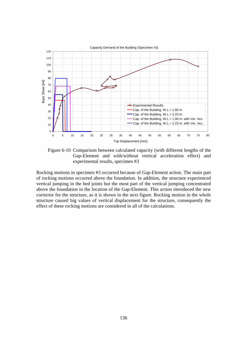
136

Capacity Demand of the Building (Specimen #3)

0

10

20

30

40

50

60

70

80

90

100

110

120

0 5 10 15 20 25 30 35 40 45 50 55 60 65 70 75 80

Top Displacement [mm]

Bas

e S

hear

[kN

]

Experimental ResultsCap. of the Building, W.L.= 1.90 mCap. of the Building, W.L.= 2.23 mCap. of the Building, W.L.= 1.90 m, with Ver. Acc.Cap. of the Building, W.L.= 2.23 m, with Ver. Acc.

Figure 6-10 Comparison between calculated capacity (with different lengths of the

Gap-Element and with/without vertical acceleration effect) and experimental results, specimen #3

Rocking motions in specimen #3 occurred because of Gap-Element action. The main part of rocking motions occurred above the foundation. In addition, the structure experienced vertical jumping in the bed joints but the most part of the vertical jumping concentrated above the foundation in the location of the Gap-Element. This action introduced the new corrector for the structure, as it is shown in the next figure. Rocking motion in the whole structure caused big values of vertical displacement for the structure, consequently the effect of these rocking motions are considered in all of the calculations.

137

Figure 6-11 Rocking motion in the Gap-Element caused noticeable vertical

displacement, specimen #3 Figure 6-12 shows the calculated capacity of the structure in comparison with the demand diagrams for specimen #3. Demand diagrams of specimen #3 are continued to 10 mm as a top displacement, but the real behavior of the structure as it is shown in Figure 6-10 was more than those calculated values. The modal approach parameters are given in Table 6-4:

Table 6-4 Modal approach parameters for specimen #3

Storey Level 1 Level 2 Mass [to] 10.00 8.24

Height [m] 2.07 4.17 First mode distribution 0.5 1.0

Required data for the conversion of M.D.O.F. to S.D.O.F.:

E i iM m φ= ⋅∑ = 13.24 to

i i iE

i i

h mh

mφφ

⋅ ⋅=

⋅∑∑

= 3.38 m

2i i

i i

mm

φφ⋅

Γ =⋅

∑∑

= 1.23

138

Capacity Demand of the Building, Specimen #3

0

50

100

150

200

250

300

350

0 2 4 6 8 10 12 14 16 18 20Top Displacement [ mm ]

Bas

e Sh

ear [

kN

]

Test 3-2, Damping 3%Test 3-4, Damping 3%Test 3-6, Damping 3%Test 3-8, Damping 3%Test 3-10, Damping 3%Test 3-12, Damping 3%Test 3-14, Damping 3%Test 3-16, Damping 3%Test 3-18, Damping 3%Test 3-20, Damping 6%Test 3-22, Damping 6%Test 3-24, Damping 6%Test 3-26, Damping 6%Test 3-28, Damping 6.1%Test 3-30, Damping 6.3%Test 3-32, Damping 6.7%Test 3-34, Damping 7%Cap. of the Buil., W.L.= 1.90 mCap. of the Buil., W.L.= 2.23 mCap. of the Buil., W.L.= 1.9 m, with Ver. Acc.Cap. of the Buil., W.L.= 2.23 m, with Ver. Acc.

Figure 6-12 Performance point according to the calculated capacity curves of the

building and demand diagrams for specimen #3 Figure 6-13 has the same rule like Figure 6-8 but for specimen #3. As it is shown in this figure with the real values of the damping the demand point in the last test is matched with the requested capacity from the demand diagrams. The calculations proved ductile behavior of the structure until the last test 3-34.

Capacity Demand of the Building, Specimen #3

0

50

100

150

200

250

300

350

0 10 20 30 40 50 60 70 80 90 100Top Displacement [ mm ]

Bas

e Sh

ear [

kN

]

Test 3-2, Damping 3%Test 3-4, Damping 3%Test 3-6, Damping 3%Test 3-8, Damping 3%Test 3-10, Damping 3%Test 3-12, Damping 3%Test 3-14, Damping 3%Test 3-16, Damping 3%Test 3-18, Damping 3%Test 3-20, Damping 6%Test 3-22, Damping 6%Test 3-24, Damping 6%Test 3-26, Damping 6%Test 3-28, Damping 6.1%Test 3-30, Damping 6.3%Test 3-32, Damping 6.7%Test 3-34, Damping 7%Cap. of the Buil., W.L.= 1.90 mCap. of the Buil., W.L.= 2.23 mExperimentalCap. of the Buil., W.L.= 1.90 m, with Ver. Acc.Cap. of the Buil., W.L.= 2.23 m, with Ver. Acc.

Figure 6-13 Capacity criteria comparison between real values, expected and

calculated results, specimen #3

139

6.2.2 Calculation of Behavior Factor This section shows numeric values of ductility in order to compare with DIN-Code. A range of values of q factor (behavior factor) for different systems of masonry structures is proposed in prEN 1998-1:

• For unreinforced masonry: 1.5 2.5q= − • For confined masonry: 2.0 3.0q= − • For reinforced masonry: 2.5 3.0q= − .

The calculated displacement ductility for both specimens is shown in Table 6-5 (according to the tabulated data in Table 5-2 and Table 5-3). The displacement ductility is given by the following equation:

U

Y

UltimatedisplacementYield displacement

μ Δ= =

Δ (6.2.15)

• Following the hypothesis of equal displacements, the behavior factor q equals

the value of the ductility μ , • But there is other method to evaluate the level of maximum forces according to

the hypothesis of equal deformation energy as is depicted in Figure 6-14 [46]:

Figure 6-14 Deformation energy method for evaluating the level of maximum

forces ΔY [mm]: Yield displacement, Table 5-2, test 1-12 for specimen #1 and Table 5-3, test 3-10 for specimen #3, ΔU [mm]: Ultimate displacement, Table 5-2 and Table 5-3,

140

yF [kN]: Load; average base shear in ductile mode, adopted from Table 5-2 (test 1-2 to test 1-22) for specimen #1 and Table 5-3 (test 3-12 to test 3-34) for specimen #3,

elF [kN]: Maximum elastic load is calculated from equal areas in Figure 6-14. These values correspond very well with the elastic response shear force according to the response spectra in Figure 6-8 and Figure 6-13.

Table 6-5 Ductility for achieved tests

Specimen

ΔY [mm]

ΔU [mm]

Displacement Ductility

yF

[kN]

Area (OADE)

[kN . mm]

elF [kN]

Behavior Factor q

1 10.7 29.5 2.8 66.3 1567.2 139.1 2.1 3 10.8 75.1 7.0 75.6 4529.4 252.0 3.3

6.3 Stress Criteria Shear stress distribution can be as suitable criteria for approving the accuracy of experimental investigation. This section is investigated on shear stress distribution in the specimens. In further figures the shear stresses criteria in both specimens are shown, concerning the shear stress distribution it is realized why the specimen #3 (with Gap-Element) could resist with more than double base acceleration in comparison with specimen #1 (without Gap-Element), see Table 5-1.

6.3.1 Shear Stress Criteria for Experimental Investigations Shear stress distribution shows acceptable evaluation for understanding the behavior of the specimens during the seismic loads. For producing a shear capacity diagram, there are three separated parts diagrams are required. The first is demand force by attention to the DIN requirement or Schubert research results and the second one is the presented shear capacity of the wall calculated during experimental tests, third part is theoretical shear force according to the different eccentricities ( /Q e N h= ⋅ ) (or the line that introduces stability condition of the structure for different values of eccentricity). For calculating the DIN requirement approach, following procedures are needed: 1. Consider a wall with: t = thickness, d = length, h = height, N = normal force, Q =

shear force, 2. Specify different values of eccentricity e ; (logic evaluation gives further values for

eccentricities by attention to the length of the wall d consequently / 6 / 2d e d< < ),

3. Evaluate the length of the compressive area on foundation x with equation:

3 / 2 3x d e= ⋅ − ⋅ (6.3.1)

141

4. Calculate maximum compressive stress in masonry by:

max2 . . ( )

. .

⋅= < ⋅

⋅⋅ =

N Admiss Comp Stress Safety Factorx t

Redistribution Factor Ult Comp Stress

σ γ (6.3.2)

5. Calculate ultimate shear stress maxτ with below conditions:

maxmax

maxmin

0.2 ( 1/ 2 )NSt

zul OHS DM

nτ βτ γ

τ σ σ σ= ⋅⎧

= ⋅ ⎨ = + ⋅ = ⋅⎩ (6.3.3)

6. Maximum ultimate shear force is:

max max

1.5; / 2/ ;

1.0; / 1h d

Q x t c ch d

τ≥⎧

= ⋅ ⋅ = ⎨ ≤⎩ (6.3.4)

Table 6-6 shows the required parameters according to the DIN code and materials used.

Table 6-6 Data for evaluating shear stress criteria from DIN code

Achieved Test

Specimen #1

Specimen #3

Type of Brick HLZ / 12 HLZ / 12 Type of Mortar IIa DM

n 0.012 0.012 NStβ 12 12

OHSσ 0.09 0.11 Admissible Compressive Stress 1.6 2.2

Safety Factor γ 2.0 2.0 Redistribution Factor * 1.3 1.3

Ultimate Compressive Stress 4.16 5.72 * DIN 1053-1 Section 7.2.3, see [51]

For evaluating the shear capacity of the walls according to Schubert [13] values, the following procedures must be operated: 1. Maximum acceptable shear stress:

max

0.08; /12 , 1/ 2

0.32vk x x DM

af a b for HLZ

bσ σ σ σ

=⎧= + ⋅ = = ⋅⎨ =⎩

(6.3.5)

142

The parameter maxσ is given by equation 6.3.2 2. Maximum acceptable shear force is:

Rd vkQ f x t= ⋅ ⋅ (6.3.6) Length of compressive zone x is given by equation 6.3.1. Simple static calculations need to show theoretical shear force according to the assumed eccentricity and existing vertical load, hence:

/Q e N h= ⋅ (6.3.7) Figure 6-15 shows three diagrams according to DIN, Schubert [13] and maximum theoretical eccentricity (= length of the wall / 2). This figure shows over estimation of shear capacity from Schubert values in comparison with DIN evaluations, on the other hand both diagrams show failure points of shear capacity around maximum eccentricity (d / 2 = 2.23 / 2 = 1.12 m). For finding out the demand point and the best design of any structure, theoretical shear force of the structure has to be generated (stability line). In order to produce this line, the equivalent height of the structure is required. The equivalent height of the structure is calculated in previous section equation 6.2.12:

3.47Eh = m

Shear Capacity Criteria, Specimen #1

0

50

100

150

200

250

0 0.1 0.2 0.3 0.4 0.5 0.6 0.7 0.8 0.9 1 1.1 1.2

Eccentricity e [m]

Max

imum

Hor

izon

tal F

orce

[kN

]

Shear Capacity (DIN)

Shear Capacity (Schubert)

Figure 6-15 Shear capacity criteria according to DIN requirements and Schubert

research, specimen #1

143

Shear Capacity Criteria, Specimen #1

0

50

100

150

200

250

0 0.1 0.2 0.3 0.4 0.5 0.6 0.7 0.8 0.9 1 1.1 1.2

Eccentricity e [m]

Max

imum

Hor

izon

tal F

orce

[kN

]

Shear Capacity (DIN)

Shear (Q=e.N/h)

Shear Capacity (Schubert)

Maximum Theoretical Eccentricity

Figure 6-16 Shear capacity criteria (DIN / Schubert) in comparison with theoretical

shear force ( /Q e N h= ⋅ ), specimen #1 Figure 6-16 shows the demand points according to the capacity of the structure for specimen #1, as it is cleared, the structure cannot bear high magnitudes of eccentricities with sufficient shear values. For example the best design could be about maximum 70 cm eccentricity and 65 kN shear force resistance. However, there is a small gap between reality and theoretical calculation. This gap exposed in Figure 6-17 when the experimental results are included to the diagrams in Figure 6-16. The experimental results follow approximately the line of theoretical shear force with upper bond values. Experimental results depicted some values for eccentricities (near 1.1 m). In the last tests of experimental results, the shear capacity of the structure remained around 70 kN, and as it is explained before the structure paid this extra excitation with its ductility. All dynamic effects are included in the experimental results calculation, such effects like vertical accelerations of floors or rotational moment in floors, Figure 6-17:

144

Shear Capacity Criteria, Specimen #1

0

50

100

150

200

250

0 0.1 0.2 0.3 0.4 0.5 0.6 0.7 0.8 0.9 1 1.1 1.2

Eccentricity e [m]

Max

imum

Hor

izon

tal F

orce

[kN

]

Shear Capacity (DIN)

Shear (Q=e.N/h)

Shear Capacity (Schubert)

Shear (All Dynamic Effects)

Maximum Theoretical Eccentricity

Figure 6-17 Shear capacity criteria (DIN / Schubert) in comparison with theoretical

shear force ( /Q e N h= ⋅ ) and experimental results, specimen #1 Some differences are revealed in these diagrams. There is a small difference between theoretical shear force of the structure and the real values from experimental tests. The theoretical shear force calculation is based on linear behavior of the structure in static case by attention to the equivalent height and total mass but specimen #1 experienced nonlinearity in seismic load, and then as it is shown in Figure 6-17 the structure desired a higher values of shear to achieve the same values of eccentricity or better to call it overturning moment (or acted load). The reason has to be focused on ductility, also masonry inherently is brittle material but some low values of ductility occurred (see table 6-3). Figure 6-17 is a complete reference for shear capacity criteria with all explained considerations.

145

Figure 6-18 Three-dimensional diagram, shear force and eccentricity vs. maximum

table excitation, specimen #1 Figure 6-18 depicts shear force (all dynamic effects) vs. eccentricity in comparison with maximum table excitation. As it is shown in this figure while structure achieved its maximum theoretical eccentricity (d / 2 = 1.12 m) then tried to carry extra load with available ductility (see Table 6-3). Also ductility of specimen #1 is not big value but structure used that ductility until last test with table excitation 5.394 m / s² (see Table 5-1). After achieving maximum eccentricity the generated total shear in structure remained around 70 kN until final failure. Same procedures are needed for evaluating the shear capacity of specimen #3. Figure 6-19 and Figure 6-20 show the multi diagram of shear capacity criteria for specimen #3 with different types of wall-length. The equivalent height is:

3.38Eh = m Figure 6-19 shows specimen #3 with a wall-length of 1.90 m and Figure 6-20 shows the same calculation in a diagram for a wall-length of 2.23 m.

146

Wall Shear Capacity Criteria for Specimen #3 (Section II-II, Wall-length 1.90 m)

0

50

100

150

200

250

0 0.1 0.2 0.3 0.4 0.5 0.6 0.7 0.8 0.9 1 1.1 1.2 1.3 1.4

Eccentricity e [m]

Max

imum

Hor

izon

tal F

orce

[ kN

]

Shear Capacity (DIN)

Shear (Q=e.N/h)

Shear Capacity (Schubert)

Shear (All Dynamic Effects)

Maximum Theoretical Eccentricity

Figure 6-19 Shear capacity criteria(DIN / Schubert) in comparison with theoretical

shear force ( /Q e N h= ⋅ ) and experimental results, specimen #3 (wall-length 1.90 m)

Wall Shear Capacity Criteria for Specimen #3 (Section I-I, Wall-length 2.23 m)

0

50

100

150

200

250

300

0 0.1 0.2 0.3 0.4 0.5 0.6 0.7 0.8 0.9 1 1.1 1.2 1.3 1.4 1.5Eccentricity e [m]

Max

imum

Hor

izon

tal F

orce

[ kN

]

Shear Capacity (DIN)

Shear (Q=e.N/h)

Shear Capacity (Schubert)

Shear (All Dynamic Effects)

Maximum Theoretical Eccentricity

Figure 6-20 Shear capacity criteria(DIN / Schubert) in comparison with theoretical

shear force ( /Q e N h= ⋅ ) and experimental results, specimen #3 (wall-length 2.23 m)

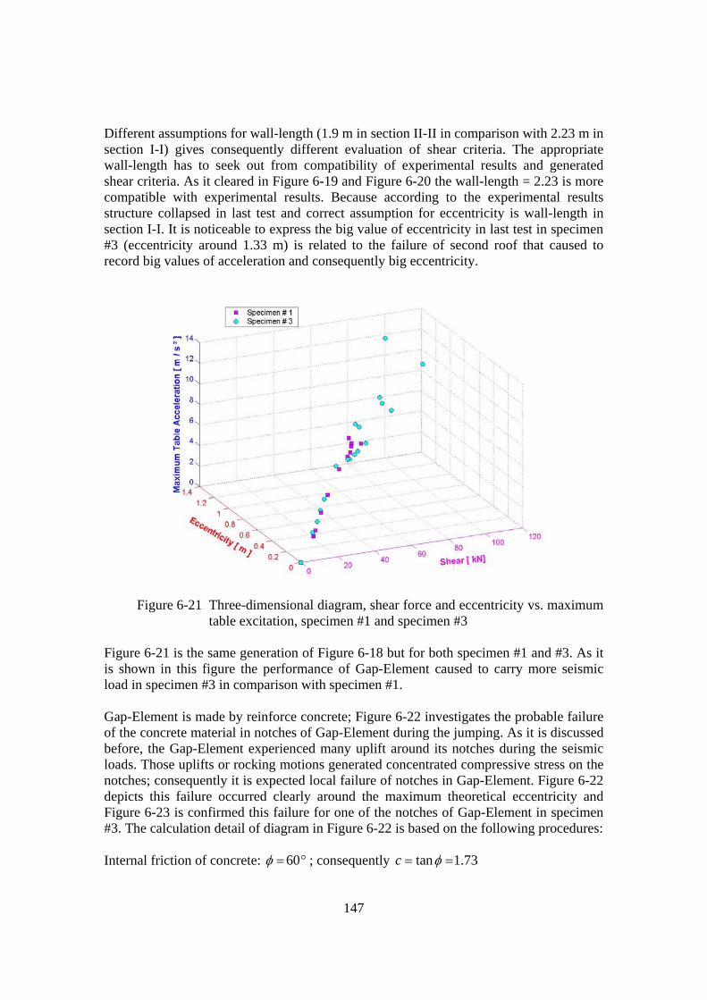
147

Different assumptions for wall-length (1.9 m in section II-II in comparison with 2.23 m in section I-I) gives consequently different evaluation of shear criteria. The appropriate wall-length has to seek out from compatibility of experimental results and generated shear criteria. As it cleared in Figure 6-19 and Figure 6-20 the wall-length = 2.23 is more compatible with experimental results. Because according to the experimental results structure collapsed in last test and correct assumption for eccentricity is wall-length in section I-I. It is noticeable to express the big value of eccentricity in last test in specimen #3 (eccentricity around 1.33 m) is related to the failure of second roof that caused to record big values of acceleration and consequently big eccentricity.

Figure 6-21 Three-dimensional diagram, shear force and eccentricity vs. maximum

table excitation, specimen #1 and specimen #3 Figure 6-21 is the same generation of Figure 6-18 but for both specimen #1 and #3. As it is shown in this figure the performance of Gap-Element caused to carry more seismic load in specimen #3 in comparison with specimen #1. Gap-Element is made by reinforce concrete; Figure 6-22 investigates the probable failure of the concrete material in notches of Gap-Element during the jumping. As it is discussed before, the Gap-Element experienced many uplift around its notches during the seismic loads. Those uplifts or rocking motions generated concentrated compressive stress on the notches; consequently it is expected local failure of notches in Gap-Element. Figure 6-22 depicts this failure occurred clearly around the maximum theoretical eccentricity and Figure 6-23 is confirmed this failure for one of the notches of Gap-Element in specimen #3. The calculation detail of diagram in Figure 6-22 is based on the following procedures: Internal friction of concrete: 60φ = ° ; consequently tan 1.73c φ= =

148

Ultimate compressive stress of concrete: Ultimateσ = 30 MPa Eccentricity: e Length of the concrete beam: l Length of the compressive stress area (plasticity theory): 2x l e= − ⋅ Vertical load: N Normal stress: /N N t xσ = ⋅ Shear stress: 0 Ncτ σ σ= + ⋅

Principal stress: ( ( )2 21 / 2 / 2) / 2N Nσ σ σ τ= + +

Then for generating the diagram in figure 6-21 the principle stress is given by:

1 1

1 0.0Ultimate

Ultimate

ififσ σ σσ σ

< ⇒⎧⎨ ≥ ⇒⎩

Concrete Shear Capacity Criteria for Specimen #3 (Section II-II, Wall-length 1.90 m)

0

5

10

15

20

25

30

35

0 0.1 0.2 0.3 0.4 0.5 0.6 0.7 0.8 0.9 1Eccentricity e [m]

Prin

cipl

e St

ress

[ M

N /

m² ] Concrete Failure

Maximum Theoretical Eccentricity

Figure 6-22 Concrete failure criteria for Gap-Element notches

149

Figure 6-23 Failure of the notches in Gap-Element caused by concentrated compressive stress, specimen #3

6.3.2 Collapse Evaluation of Specimen #3 Specimen #3 could carry the seismic load until 12 m/s2 excitation but finally failure of the second floor caused to finish the test. The behavior of Gap-Element and noticeable values of jumping for whole of the structure have to consider in evaluating the collapse of the specimen #3. Two aspects have to study for evaluating the collapse reasons:

1. Shear failure like failure of specimen #1 in last test, 2. Pounding effect of second floor during the return movement to the neutral

position. For answering these questions, it is needed to repeat same procedures in previous section in order to evaluate the behavior of the structure during the seismic loads. Figure 6-24 shows multi diagrams of shear capacity criteria for second floor in specimen #3. The level of all eccentricity calculations is above the first roof and this level is considered as a fix support. As it is expected the second floor has to fail in last test with eccentricity bigger than the allowable eccentricity (2.23 / 2 = 1.115 m).

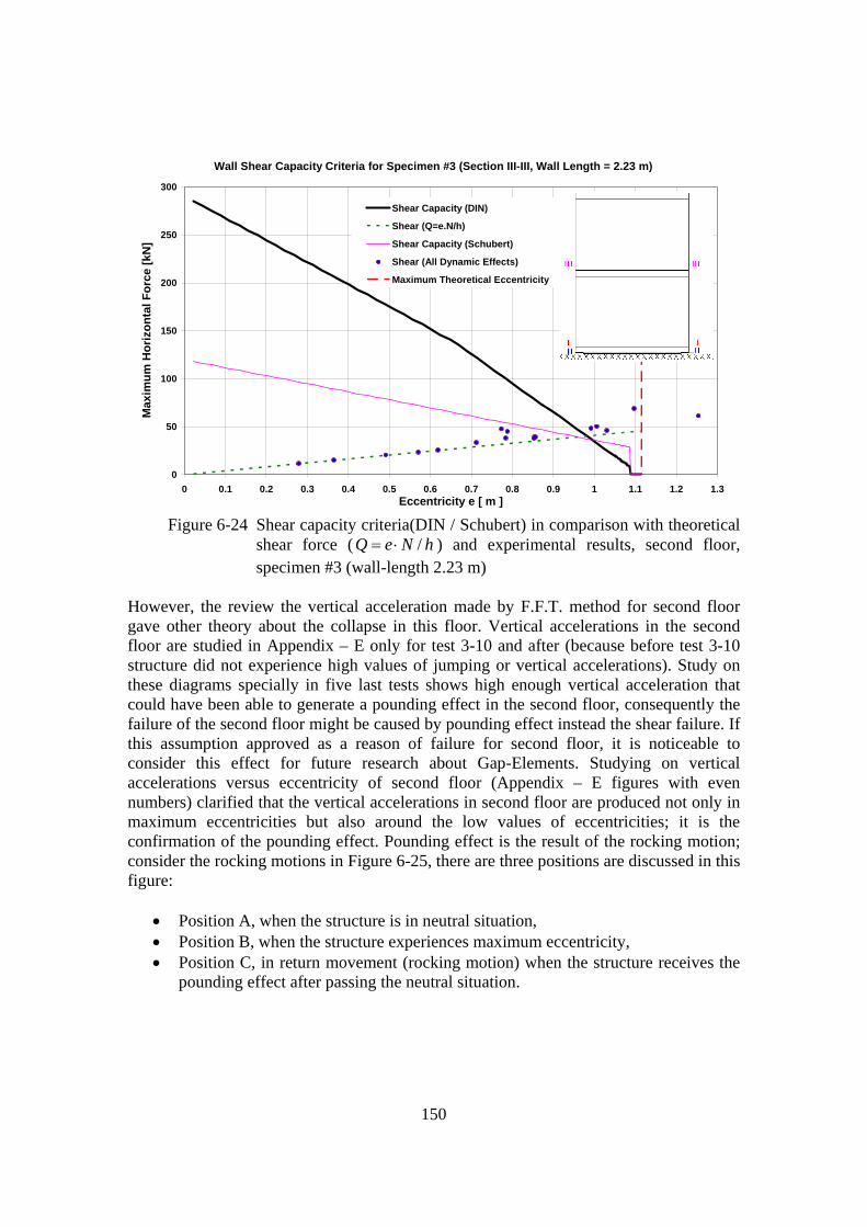
150

Wall Shear Capacity Criteria for Specimen #3 (Section III-III, Wall Length = 2.23 m)

0

50

100

150

200

250

300

0 0.1 0.2 0.3 0.4 0.5 0.6 0.7 0.8 0.9 1 1.1 1.2 1.3Eccentricity e [ m ]

Max

imum

Hor

izon

tal F

orce

[kN

]

Shear Capacity (DIN)

Shear (Q=e.N/h)

Shear Capacity (Schubert)

Shear (All Dynamic Effects)

Maximum Theoretical Eccentricity

Figure 6-24 Shear capacity criteria(DIN / Schubert) in comparison with theoretical

shear force ( /Q e N h= ⋅ ) and experimental results, second floor, specimen #3 (wall-length 2.23 m)

However, the review the vertical acceleration made by F.F.T. method for second floor gave other theory about the collapse in this floor. Vertical accelerations in the second floor are studied in Appendix – E only for test 3-10 and after (because before test 3-10 structure did not experience high values of jumping or vertical accelerations). Study on these diagrams specially in five last tests shows high enough vertical acceleration that could have been able to generate a pounding effect in the second floor, consequently the failure of the second floor might be caused by pounding effect instead the shear failure. If this assumption approved as a reason of failure for second floor, it is noticeable to consider this effect for future research about Gap-Elements. Studying on vertical accelerations versus eccentricity of second floor (Appendix – E figures with even numbers) clarified that the vertical accelerations in second floor are produced not only in maximum eccentricities but also around the low values of eccentricities; it is the confirmation of the pounding effect. Pounding effect is the result of the rocking motion; consider the rocking motions in Figure 6-25, there are three positions are discussed in this figure:

• Position A, when the structure is in neutral situation, • Position B, when the structure experiences maximum eccentricity, • Position C, in return movement (rocking motion) when the structure receives the

pounding effect after passing the neutral situation.

151

Figure 6-25 Pounding effect in second floor of specimen #3

There are two possibilities for evaluating the failure reasons:

• First, structure failed in position B because of receiving its maximum eccentricity and consequently crashed on that situation,

• Second, structure does not fail in position B rather it fails in position C because of uplift in the second floor and consequently it loses its shear capacity (stiffness).

The second possibility will deny because in position C there is not enough eccentricity to produce the shear force (consequently shear failure), on the other hand the data processing in specimen #3 confirmed that the failure occurred in position B and the time step of this failure was before to receive the highest values of vertical acceleration in position C. It means structure collapsed in position B and after that failure with high values of eccentricities returned to the position A and after switched to the position C and receiving big values of vertical acceleration (made by pounding effect) and after the excitation passes its lower magnitudes and the test is finished (because of big failure in the walls of the second storey), see Table 6-7 and Figure 6-26.

152

Table 6-7 Time table of maximum eccentricity (total, second floor), specimen #3

Test Number

Time of Total Eccentricity

[S]

Total

Eccentricity [m]

Time of 2-Fl. Eccentricity

[S]

2-Floor

Eccentricity [m]

Time of Maximum Vertical

Acceleration [s] 2 3.76 0.35 3.67 0.28 2.53 4 3.76 0.46 3.77 0.36 3.06 6 3.77 0.59 3.78 0.49 1.69 8 3.78 0.67 3.79 0.57 4.86 10 4.00 0.87 4.00 0.62 3.99 12 4.02 0.99 4.22 0.71 4.22 14 4.04 0.92 4.03 0.85 4.27 16 4.05 0.91 4.03 0.86 4.29 18 4.04 0.89 4.04 0.78 4.30 20 4.06 0.87 4.04 0.85 4.32 22 2.96 0.97 2.96 0.99 2.94 24 2.18 0.96 2.95 1.03 3.84 26 4.05 0.88 4.05 0.79 2.18 28 3.86 0.86 3.85 0.77 4.07 30 3.40 0.90 3.40 1.01 3.44 32 2.16 1.07 2.14 1.10 2.12 34 1.98 1.34 2.18 1.25 3.41

Figure 6-26 is the comparison of total eccentricities of the specimen #3 in test 3-34 (last test) with vertical accelerations of the second floor. The maximum vertical acceleration of the second floor is occurred in low values of eccentricity (around 40 cm); it is the position C in Figure 6-25. Figure 6-27 shows shear criteria and effect of the eccentricity on the second floor in test 3-28. This figure is calculated only for absolute values of the generated shear in second floor and it is compared these shear values with Schubert results and DIN evaluations for shear capacity in the second floor (only absolute of eccentricities are considered). Lack of any meeting-point in these diagrams in Figure 6-27 means safe behavior of the second floor against the acting seismic load in test 3-28. Figure 6-24 shows for the eccentricity around 0.77 m (see Table 6-7, test 3-28, 2-Floor eccentricity) the value of Schubert diagram is 50 kN instead DIN that gives approximately 125 kN for shear capacity of the second floor. The generated shear in second floor during whole of the loading in test 3-28 is less than 50 kN; this is the reason the seismic tests continued with higher values of excitations.

153

Shear force in 2-Floor Specimen #3, test (28)

0

25

50

75

100

125

150

175

200

225

250

275

300

0.0 1.0 2.0 3.0 4.0 5.0 6.0 7.0 8.0 9.0Time [s]

Shea

r For

ce [k

N]

Shear Force (Absolute Values)

Schubert

DIN

Specimen #3, Test (34)

-1.50

-1.00

-0.50

0.00

0.50

1.00

1.50

-6.00 -4.00 -2.00 0.00 2.00 4.00 6.00 8.00Vertical Acceleration of Second Floor [m/s²]

Ecce

ntric

ity T

otal

[m]

Figure 6-26 Total eccentricity vs. vertical acceleration of second floor, test 3-34

Figure 6-27 Time history of shear failure in second floor according to the DIN, Schubert vs. shear force , test 3-28

154

Figure 6-28 is like the Figure 6-27 but for test 3-34 in specimen #3. After second 2 (around 2.18 s see Table 6-7, time of the second floor eccentricity) the generated shear in the second floor is 62 kN and this value is bigger than the shear capacity of the second floor according to the both shear criteria evaluations (Schubert, DIN), see Figure 6-24.

Figure 6-28 Time history of shear failure in second floor according to the DIN,

Schubert vs. shear force , test 3-34

155

7 CONCLUSION AND SUGGESTIONS

7.1 Introduction This chapter gives a final overview of the tests performed on three specimens including conclusions and suggestions for further researches. The data obtained from the experiments have been processed and evaluated. Additional theoretical investigations have helped to understand the behavior of walls with Gap-Elements. It could be demonstrated that due to the Gap-Element a masonry wall is able to carry high magnitude excitations.

7.2 Conclusions The conclusions consist of three parts; first, the conclusions from experimental tests; second, the conclusions from analytical investigations and third, general conclusions.

7.2.1 Conclusions Concerning the Experimental Tests In Chapter 5, the methodology for experimental investigations is discussed in detail. The following conclusions can be drawn:

• During the experimental investigations, a significant amount of information has been obtained from deformation and acceleration sensors. However, no vertical accelerometers had been installed on the specimens. For this reason, vertical accelerations are calculated by using numerical methods (F.F.T. method using the recorded vertical displacements). So, some inaccuracy in the generated vertical acceleration data could not be avoided. In further research it is advised to set up vertical accelerometers in order to record the vertical responses of the structure,

• Since specimen #2 rules as a prototype sample, the only possibility to investigate the behavior of Gap-Element experimentally is limited to specimen #3. Hence, it seems necessary to perform further experiments with walls using Gap-Elements,

• The steel strips (see Figure C-9-a) as used for specimen #3 could be advantageous generally in order to limit tensile stresses and strains inside the masonry wall. Further research should be carried out in order to study the effect of such steel strips or equivalent reinforcement of the wall edges on the dynamic responses of walls with Gap-Elements,

• In comparison with normal mortar, the thin layer mortar in specimen #3 did not have a big influence in whole on the seismic response of the structure,

• No mortar had been implemented in the vertical joints (head joints) of the test specimens. The effect of filling the vertical joints with mortar could, however, be

156

noticeable in seismic response of the structure; especially with the smaller size of the bricks.

7.2.2 Conclusions Concerning the Analytical Investigations The analytical investigations are explained in detail in Chapter 6. As it is explained in that chapter, the analytical calculations showed the compatibility between experimental and analytical results. Demand capacities and shear resistance criteria are proved by the correct matching of the selected theoretical methods with the experimental achievements. It should be noticed that the complete test results include a huge number of data (the raw data from the shaking table before processing was about 1,000,000 numerical values). Due to this complexity, the data evaluation process needed a long time and a lot of computer expenses. The analytical investigations included three parts:

1. Data processing, in order to process the generated data from the shaking table and to produce graphs or figures as they are depicted in Chapter 5 (responses of the roofs, vertical jumping, vertical acceleration, frequency domain discussion, etc);

2. Data evaluation, in order to judge the response from an engineering point of view

and in order to compare the behavior of the structure with the available design procedures (design code provisions and actual research results). Furthermore, the validity of the idea, that the Corner-Gap-Element is able to limit the maximum eccentricity of reaction forces can be checked by the evaluation of the test data. The main target of this part is to realize the responses of the structure against the applied seismic loads in order to investigate the accuracy of the selected methods or weak / strong points of the structure.

3. The failure of specimen # 3 occurred in the upper storey. The calculations showed

that the main reason for the failure was the ultimate shear capacity of the upper storey (see Figure 6-28) with influence of vertical acceleration (Section 6.3.2).

7.2.3 General Conclusion General conclusion can be listed in following points:

• Gap-Element is able to produce a quasi (fictitious) ductility making the structure resistant enough against severe earthquakes. In other words; the Gap-Element has the same role like a ductile link in ductile chain design criteria (see Section 2.5.1.2) in whole of the unreinforced masonry tested structure, Figure 7-1:

157

Figure 7-1 Performance of specimen #3 (with Gap-Element) in comparison with specimen #1 (without Gap-Element)

• Specimen #3 has shown that the Gap-Element could be an effective and cheap

method to improve the seismic behavior of masonry structures. • No special training is required for the bricklayers due to the simple construction

process. • The experimental results validate the usability of the Gap-Element to increase the

seismic resistance of masonry structures. • More investigations are needed to confirm the rules for using the Gap-Elements in

the market. • In order to avoid premature failure in upper storeys, it should be conceived to

install Gap-Elements in each storey rather than only one layer with Gap-Elements above the foundation, but pounding effect has to be studied carefully.

• The response of the Gap-Element during the seismic loading has shown, using the approach presented in this paper, it is possible to improve the seismic response of the structures without any enhancements like steel frame, concrete members (or reinforcement in the mortar or bricks) in the masonry structures (or other brittle structure like adobe structures).

• The real behavior of any structure during earthquakes requires to perform earthquake simulation tests, e.g. on a shaking table, although with nowadays technologies there is the ability of modeling structures in the computer. For walls with Corner-Gap-Elements, however, modeling the structures on the shaking table has been proven to be the best way for modeling and evaluating seismic responses

158

of the structure, since the effects of vertical jumping and vertical inertia forces can be studied very well.

• Ductile chain design can be the key point to establish new methods for improving the dynamic responses of brittle structures, like masonry or adobe.

7.3 Gap-Element in Further Research As it is mentioned in the experimental tests, the Gap-Element has the ability to push away structures from earthquake loading hazard with an acceptable safety factor, without any hard crash in walls or discontinuity in bricks. Future research work may focus on this idea, especially on the following categories:

• Use the Gap-Element in orthogonal directions in order to capture both sides of the structure under seismic loading,

• Use the Gap-Element in upper storeys to establish the same system like in the first storey,

• Use the Gap-Element with another type of structures like steel or concrete structures,

• Use the Gap-Element in long span structures like bridges as a foundation for each column,

• Study on specimens with Gap-Element with / without steel strip or other reinforcements at the wall edges in order to investigate the influence of steel strip on the Gap-Element behavior,

• Study on Gap-Element in 3D-excitations in order to investigate the behavior of this element on those categories of seismic loads,

• Study on behavior of Gap-Element with different types of time histories, for example investigate with longer time histories especially for other regions with different types of earthquakes,

• Study on other different types of sliding stopper (Appendix - C, Figure C-9-b) to avoid the sliding in Gap-Element in order to increase as much as possible the performance of Gap-Element especially in upper storeys, or in orthogonal Gap-Element for both horizontal directions,

• Investigate the combination of Corner-Gap-Elements with damping / visco-elastic elements in order to limit the impact effect occurring during joint closing,

• Layout of connection joints or separating joint respectively between orthogonal walls.

7.3.1 Suggestions for Improvements in Test Methodology During these research activities, some observations made us to suggest the following points for further researches in order to have a better evaluation of the tests and their results:

159

• Use high-speed shutter video camera in order to record the responses of the structure during the seismic loading in different sides of the specimens, and investigate on the structure’s behavior. For example with high speed shutter video camera, it is possible to study on the vertical discontinuity of the mortar in the bed joint, in order to realize the weak point of the Gap-Element, especially in the building with Gap-Element in upper storeys,

• Install vertical accelerometers on the structure in order to record vertical accelerations of the structure,

• In case of possible, use laser LVDT´s or accelerometers in order to record data with high accuracy.

7.3.2 Gap-Element in Practice The performance of the Gap-Element on the shaking table has met the expectations. Preliminary design recommendations could be developed on the basis of the test results and the accompanying analytical investigations. However, in order to use the Gap-Element in practice, more tests on earthquake simulators are required. More specimens with different materials with varied types of structures have to be investigated. Gap-Elements may be used for masonry walls in orthogonal directions. This, however, requires the condition of tests under biaxial excitation. Gap-Elements may also be used for strengthening / repair or seismic upgrading of existing structures. For this purpose, the installation of Gap-Elements in more than one storey may be conceived.

7.4 Key Points for preliminary Design of Gap-Element

7.4.1 Gap-Element’s Dimensions As it is mentioned in Chapter 4.2 the dimension of the Gap-Element is the preliminary design parameters that have to clarify for any kind of research project or use it in practical field. The dimensions of the Gap-Element have to specify by the following parts, Figure 7-2:

• Length of the Gap-Element: GL • Height of the Gap-Element: GH • Thickness of the Gap-Element: GT • Length of the notches: notchL • Height of the notches: notchH

160

Figure 7-2 Dimensions of Gap-Element

As it is discussed before in Chapter 4.2 the thickness and length of the Gap-Element are the same as the wall above the Gap-Element, consequently there are three dimensions left to be specified; height of the Gap-Element and dimensions of the notches (length and height). The appropriate height for the Gap-Element is the height of the bricks (if the brick’s height is more than the minimum height of the rectangular concrete beam in code, for shear stirrups minimum requirement or longitudinal reinforcement). If the height of the units has a low value, the height of the Gap-Elements should be at least 20 cm. The length of notches as it mentioned in Chapter 4.2 can be 70 % of the height of the Gap-Element. Height of the notches can be supposed between 5 % and 10 % of the Gap-Element’s height (at least 2 cm). There are two parameters to be considered in design of notch’s height:

• Minimum height for avoiding any kind of pounding between notch and foundation level, Figure 7-3,

• Minimum height for locating the sliding stopper (see Figure C-9-b for detail). For avoiding any pounding between notch and foundation level; it is necessary to calculate possible maximum overturning movement of the Gap-Element according to geometry specification of the Gap-Element. For example during of this research the maximum jumping of the Gap-Element (as it is shown in Figure 5-33) was 2.25 cm, simple calculation (see Chapter 4.2 for details) in following shows the height of the notches 2.0 cm was enough for preventing of any kind of pounding effect on the foundation level with notches, Figure 7-3:

Figure 7-3 Jumping of Gap-Element during the seismic load

161

223 cmL(G) = (Table C-6), 17.0 cm, 2.0 cmL Hnotch notch= = (see Chapter 4.2 for

details). If the Gap-Element is being considered as a rigid structural member:

2.2517.0 0.172 cm 2.0 cm223

U y (G)U L Hy (notch) notch notch

L(G)

U y (notch) = ⋅ = <<

= ⋅ ≤

Reinforcement in Gap-Element has to be designed according to the code, although there was a failure in Gap-Element’s notches in last test of specimen #3 (see Figure 6-23) but it is not necessary to consider any especial kind of reinforcement design for the Gap-Element in building with maximum 3 storeys. In this research the Gap-Element has not been investigated for especial structures such as bridges or multi direction Gap-Element. It seems however, for these kind of the structures need to design more stiff edges in the notches for preventing any crash or noticeable failure in concrete. It has to consider any big crash in the notches has side effects on the sliding stopper, because this kind of the crash cause to lose shear resistance in the Gap-Element. As a design proposal; the Gap-Element has to be designed as a rigid structural beam that is strong enough to carry the demand seismic load.

7.4.2 Limitation of Eccentricity in Corner-Gap-Element: Eccentricity is the most important aspect that has to be taken in to account in design of the Gap-Element. Maximum eccentricity depends on following structural specifications:

• Maximum vertical load, • Maximum horizontal load, • Length of the walls (or length of the Gap-Element), • Type of the loading (magnitude and frequency contents), • Number of the storeys, • Stiffness of the structure and material properties such as ductility, nonlinear

behavior, etc, • Vertical acceleration, • Time-overlapping between maximum horizontal and vertical acceleration.

Limitation of eccentricity has to be considered in the calculation not only as a control values for stability of the structure but also as a control value for architectural / economic aspects (drift control). The architectural / economic aspects that cause to control drift of the structural are depending on the several aspects, for example:

162

• The first purpose is to limit damage to nonstructural elements such as partitions, plastering, veneer, window panels and installations,

• Given a type of connection between structural and nonstructural elements, given a set of gaps between them and given a connection design for piping and other installations, there is a drift beyond which the probability of damage is very high,

• Revision of a tentative design under the action of earthquake of various intensities may indicate that despite the high likelihood of frequent nonstructural damage, the design is adequate or else that is required revision. The design should be based on economic considerations, giving proper weight to the probability of injury and loss of life from falling debris [8].

As it is shown in results; Gap-Element can carry the high values of the seismic loads if it is allowed to rock. Simple following calculation shows the method for calculating the maximum eccentricity in every Gap-Element:

• Equivalent height of the structure (from Modal Participation Factor): h • Total vertical force: N • Considering the half length of the wall as the maximum acceptable eccentricity

(Figure 6-19 and Figure 6-20 show the appropriate dimension for the wall’s length in the Gap-Element calculation is the length of the whole wall instead the length of the Gap-Element without notch’s length. In Figure 6-20 the calculated eccentricities with the length of the wall are compatible with the real data from laboratory): maxe

• Lateral force on the structure: Q • Eccentricity: max/= ⋅ ≤e Q h N e • The maximum acceptable lateral force can be determined by maximum acceptable

eccentricity value: max max /= ⋅Q e N h The maximum acceptable lateral force has to be compatible with the calculated lateral force that is obtained from capacity design approach in next section.

7.4.3 Capacity Spectra for Preliminary Design Approach in Structure with One-Directional Gap-Element

For preliminary design approach according to the capacity spectra the following listed items have to achieve [48]:

1. Calculate capacity curves values from available method as it is shown in the Section 6.2.1,

2. Estimate the viscous damping of the structure, 3. Design ductility for Gap-Element can be 5 (equal 2 times of the calculated value

from step 1; in Table 6.5, the average ductility for the Gap-Element is 5.15 and for specimen #1 is 2.43), Figure 7-4,

163

Figure 7-4 Gap-Element improves the ductility of the structure

4. Type of the response spectrum depends on the code regulations (according to the

subsoil, type of the building, etc) and has to be selected. From this, the demand diagrams (as it is explained in Section 6.2.1) and the capacity spectra (as it is shown in Figure 6-12) have to be generated,

5. Define demand point as it is shown in Figure 7-5, 6. Location of demand point shows the behavior of the structure against the selected

seismic load (step 4), there are following possibilities for any kind of the loading:

Figure 7-5 Demand point approach for designing structure with one-directional

Gap-Element in capacity design approach diagram

• Predominantly Elastic behavior of the structure and safe design approach, case A in Figure 7-5,

164

• Elasto plastic behavior of the structure and safe design by using the target ductility, case B in Figure 7-5,

• Inappropriate ductility and unsafe design that causes the collapse of the structure, case C in Figure 7-5.

7.4.4 Verification according to DIN 4149 for Preliminary Design Approach in Structure with One-Directional Gap-Element

Design approach base on the DIN 4149 includes following procedures but with specifying the Gap-Element ductility:

1. Primary elastic spectrum parameters that include: • Type of the subsoil, • Earthquake zone, • Ground acceleration, • Amplification factor, etc.

2. Select appropriate behavior factor by attention to the type of the structure and generate design response spectrum. In Table 17 from DIN 4149 [47], behavior factor q for masonry structures are given between 1.5 for unreinforced masonry to maximum value 2.5 for reinforced masonry. As it is mentioned before; the Gap-Element can produce ductility around 5. By attention to the maximum presented values from DIN 4149, it seems maximum proposed q-factor by DIN 4149 (for reinforced masonry) can be used for unreinforced masonry with Gap-Element. Using the lower value of q-factor (2.5 instead of 3.3) is providing an additional safety margin for designing the structure.

3. Generate the design response spectrum in order to evaluate the maximum response acceleration of the structure.

4. Calculate the fundamental period of the structure by using the suggested formula and rules in code.

5. Calculate the maximum base shear on the structure. 6. Distributing the maximum base shear from step 5 on the storeys level. 7. Design control that includes:

• Safety factor, • Stress check, • Stability control (maximum eccentricity), • Stiffness evaluation (design or control), • Drift control according to the height of the structure. Drift tolerance is around

0.01 x height to 0.02 x height for strong earthquakes in most earthquake codes.

8. If control procedures in step 7 did violate any code requirements then according to the case by changing the appropriate option (such structural specifications or positions of the structural member, etc) and repeating from step 4 the design approach has to continued.

Following calculations show the above procedures for specimen #3 in the worst case of earthquake action in Germany seismic hazard map:

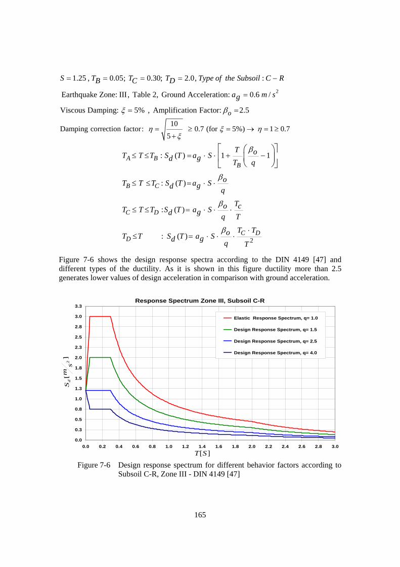
165

2

1.25 , 0.05; 0.30; 2.0, :

Earthquake Zone: III , Table 2, Ground Acceleration: 0.6 /

Viscous Damping: 5% , Amplification Factor: 2.5o

S T T T Type of the Subsoil C RB DC

a m sg

ξ β

= = = = −

=

= =

10Damping correction factor: 0.7 (for 5%) 1 0.7

5= ≥ = → = ≥

+η ξ η

ξ

2

: ( ) 1 1

: ( )

: ( )

: ( )

≤ ≤ = ⋅ ⋅ + −

≤ ≤ = ⋅ ⋅

≤ ≤ = ⋅ ⋅ ⋅

⋅≤ = ⋅ ⋅ ⋅

⎡ ⎤⎛ ⎞⎢ ⎥⎜ ⎟

⎝ ⎠⎣ ⎦A B

B

B C

C D

C DD

T oT T T S T a Sgd T q

oT T T S T a Sgd q

To cT T T S T a Sgd q T

T ToT T S T a Sgd q T

β

β

β

β

Figure 7-6 shows the design response spectra according to the DIN 4149 [47] and different types of the ductility. As it is shown in this figure ductility more than 2.5 generates lower values of design acceleration in comparison with ground acceleration.

Response Spectrum Zone III, Subsoil C-R

0.0

0.3

0.5

0.8

1.0

1.3

1.5

1.8

2.0

2.3

2.5

2.8

3.0

3.3

0.0 0.2 0.4 0.6 0.8 1.0 1.2 1.4 1.6 1.8 2.0 2.2 2.4 2.6 2.8 3.0

Elastic Response Spectrum, q= 1.0

Design Response Spectrum, q= 1.5

Design Response Spectrum, q= 2.5

Design Response Spectrum, q= 4.0

2[

]d

mS

s

[ ]T S Figure 7-6 Design response spectrum for different behavior factors according to

Subsoil C-R, Zone III - DIN 4149 [47]

166

Fundamental period of the structure:

3 / 4

3 / 4

Equation (16), DIN 4149:

, 4.26 (Table C-6), 0.051

0.05 4.26 0.15 6.661

T C H H m Ct t

T s Hz

= ⋅ = =

= ⋅ = ≡

Consequently the maximum value for acceleration will be obtained from Figure 7-6 (assuming behavior factor q ≥ 2.5):

2( 1 0.15)

1.20 /d T

S m s=

≤

There is one step for calculating the base shear on the structure:

( 1)

Equation (20), DIN4149:

Equation (15), DIN 4149: 1

Importance Factor from Table (7), DIN4149: 1.01Correction Factor: 1,0 ( if one story building is considered)

M=18200 from Table C-6

⋅= ⋅

⋅∑

= ⋅ ⋅ ⋅

=

=

d T

S Mi iF Fi b S Mj j

F S Mb

kg

λ γ

γ

λ

1.2 18200 1 1 / 1000 21.84 kN= ⋅ ⋅ ⋅ =Fb

This simple calculation shows the shear force that is proposed by DIN 4149 is lower than the real values as obtained by experiments, not only with specimen #3 with Gap-Element but also specimen #1; see Figure 6-10 and Figure 6-6. There is noticeable to evaluate the maximum force suggested by DIN 4149 on the structure without any ductile behavior of the walls, it means by selecting the q=1 from Figure 7-6 then:

2( 1 0.15)3.0 , 3 18200 1 1 / 1000 54.60kN

d Tm

sS Fb=

= = ⋅ ⋅ ⋅ =

167

References [1] Shedlock, K.M.; Pakiser, L.C.: National Earthquake Information Centre, U.S.

Geological Survey (U.S.G.S).

Follow the link: http://pubs.usgs.gov/gip/earthq1/intro.html.

[2] Hendry, W. H.: Structural brickwork, Mac-Millan Press. 1981.

[3] Moghaddam, H.: Seismic Design of Masonry Structures. 1994, ISBN 964- 6379-38-9.

[4] Ekkehard, F.: Seismic Behaviour of Capacity Designed Masonry Walls in Low Seismicity Regions. First Phase Report on Activities. February 2002.

[5] HENGER, M. & LEYDECKER, G. (Eds.) 1978 ff: Erdbeben in (der Bundesrepublik). Deutschland 1974.

Follow the link: http://www.bgr.de/quakecat/eng/ger3.htm.

[6] LEYDECKER, G.: Erdbebenkatalog für die Bundesrepublik Deutschland mit Randgebieten für die Jahre 1000 - 1981. - Geol. Jb., E 36, 3- 83, 7 Abb., 2 Tab.. Hannover 1986.

Follow the link: http://www.gfz-potsdam.de/pb2/pb24/iugg/gleydecker.html.

[7] Mehdi, Z.: Seismological Aspects of Bam (SE Iran) Earthquake of 26 December, 2003. A Preliminary Reconnaissance Report.

[8] Newmark, N.M. & Rosenblueth, E.: Fundamental of earthquake Engineering. PRENTICE-HALL, INC. Englewood Cliffs. N.J 1971.

[9] DIN 1053-1: Mauerwerk, Teil 1 Berechnung und Ausfürung, Normenausschuß Bauwesen (NABau) im DIN Deutsches Institut für Normung e.V.. Berlin November 1996.

[10] Rots, J.G.: Structural Masonry, An Experimental / Numerical Basis for Practical Design Rules. Centre for Civil Engineering Research and Codes, CUR, TNO Building and Construction Research, Rijswijk. Netherlands 1997.

[11] Ali, Sk.S. & Page, A.W.: Finite Element Model for Masonry Subjected to Concentrated Loads. ASCE Journal of Structural Engineering 114(8): 1761-1784. 1988.

[12] Drysdale, R.G.; Hamid, A.A.; Baker, L.R.: Masonry Structures Behaviour and Design. 1999.

168

[13] Schubert, P.: Auswertung von Schubversuchen an Mauerwerk aus Hochlochziegeln Kalksandsteinen, Porenbetonsteinen sowie Leichtbeton und Betonsteinen. Aachen 1999.

[14] Vigil, J.F.: This Dynamic Planet. The U.S. Geological Survey, the Smithsonian Institution, and the U.S. Naval Research Laboratory.

Follow the link: http://pubs.usgs.gov/gip/earthq1/plate.html.

[15] Schiebroek, C. J. M. (ed.): Final advice CUR program-advisory committee, PAC 4, Structural Masonry. (in Dutch).

[16] MCAA: Mason Contractors Association of America. The association was formed in 1950 and today represents the industry’s largest unions and non-union contractors. Follow the link: http://www.masoncontractors.org.

[17] Paulay, T. & Priestley, M.J.N.: Seismic design of reinforced concrete and masonry buildings. By John Wiley & Sons, Inc. 1992

[18] Schneider, H.: Tests on Shear Resistance of Masonry. Proc of 4th International Brick Masonry Conference, Paper 4.b.12. Brugge 1976.

[19] Murty, C.V.R.: Earthquake Tip 15. Indian Institute of Technology Kanpur. Kanpur India.

[20] Brandao, P.J.; Lourenco, P.B.; Barbosa, R.: Computational strategies for masonry structures. Portugal February 1996.

[21] Vitorino, D. de Castro Oliveira: Experimental and numerical analysis of blocky masonry structures under cyclic loading. October 2002.

[22] Porada, E.; with the collaboration of R. H. Dyson and contributions by C.K. Wilkinson.: The Art of Ancient Iran; Pre-Islamic Culture, the Art of Seleucids. Columbia University.

[23] Schubert, P.: The influence of mortar on the strength of masonry. Proc. 8th Int. Brick and Block Masonry Conference, eds. J.W. de Courcy, Elsevier Applied Science, p.162-174. London 1988.

[24] Pluijm, R.Van Der.: Material properties of masonry and its components under tension and shear. Proc. 6th, Canadian Masonry Symposium, eds. V.V. Neis, Saskatoon, p.675-686. Canada Saskatchewan.

[25] Biolzi, L.: Evaluation of the Compressive Strength of Masonry Walls by Limit Analysis. Journal of Structural Engineering, Vol. 114, No. 10, pp. 2179-2189. October 1988.

169

[26] Cundall, P.A.: A computer model for simulating progressive large scale movements in blocky rock systems. Proc. of the Symposium of the International Society of Rock Mechanics, Vol. 1, paper # II-8. Nancy France 1971.

[27] Ghaboussi, J.; Barbosa, R.: Three-dimensional discrete element method for granular materials. Int. J. Num. Anal. Meth. Geomech., 14, pp.451-472. 1990

[28] Pagnoni, T.: Seismic analysis of masonry and block structures with the discrete element method. Proc. 10th European Conference on Earthquake Engineering, Vol.3, pp. 1674-1694. 1994.

[29] Lemos, J. V. G. Pande et al. (eds): Computer Methods in Structural Masonry-5. Discrete element modelling of the seismic behaviour of stone masonry arches. E&FN Spon, pp.220-227. London 1998.

[30] Sincraian, G. E.: Seismic behaviour of blocky masonry structures. A discrete element method approach. Ph.D. Dissertation, IST. Lisbon Portugal 2001.

[31] Meskuris, K.; Butenweg, C.; Mister, M.; Kuhlmann, W.: Seismic Behaviour of Historic Masonry Building. Chair of Structural Static and Dynamics, RWTH Aachen University. Germany.

[32] Hamid A.A.; Drysdale, R.G.: Concrete Masonry under Shear and Compression Along Mortar Joints. ACI Journal, Vol.77, No.5, pp. 51-64. September 1981.

[33] Hamid, A.A.; Drysdale, R.G.: Behaviour of Brick Masonry under Combined Shear and Compression Loading. In Proceedings of the Second Canadian Masonry Symposium, pp. 51-64. Ottawa 1980.

[34] Hamid, A.A.; Drysdale, R.G.; Heidebrecht, A.C.: Shear Strength of Concrete Masonry Joints. Journal of the Structural Division, Proceeding of ASCE, Vol. 105, ST7, pp. 106-113. July 1979.

[35] Yokel, F.; Fattal, G.: Failure Hypothesis for Masonry Shear Walls. Journal of the Structural Division, Proceedings of ASCE, ST3, Vol. 102, pp. 515-532. March 1976.

[36] Fehling, E.; Görgülü, Ü.: Computational Modelling of Masonry. Report in SAFERR Research Training Program, Kassel University. Unpublished manuscript. Germany January 2004.

[37] Shrive, N.G.; Masia, M.J.; Lissel, S.L.: Strengthening and rehabilitation of masonry using fibber reinforced polymers. University of Calgary, Department of Civil Engineering. Calgary Alberta Canada 2001.

[38] Bachmann, H.; Lang, K.: Zur Erdbebensicherung von Mauerwerksbauten. Institut für Baustatik und Konstruktion, ETH; IBK Berichr Nr. 274. Zürich May 2002.

170

[39] Lang, K.: Seismic vulnerability of existing buildings. Institut für Baustatik und Konstruktion, ETH; IBK Berichr Nr. 273. Zürich March 2002.

[40] Grünthal, G.; Mayer-Rosa, D.; Lenhardt, W.A.: Abschätzung der Erdbebengefährdung für die D-A-CH-Staaten - Deutschland, Österreich, Schweiz. Bautechnik 75, 10, 753-767, Verlag Ernst & Sohn. Berlin 1998.

[41] Grünthal, G.; Bosse, Ch.; Mayer-Rosa, D.; Rüttener, E.; Lenhardt, W.; Melichar, P.: Joint seismic hazard assessment project for Austria, Germany, and Switzerland. Duma (Ed.): Proceedings of the 10th European Conference on Earthquake Engineering, Vienna, 28 Aug. - 2 Sept., Balkema, 57-62. Rotterdam 1995.

[42] Grünthal, G.; Bosse, Ch.: Probabilistische Karte der Erdbebengefährdung der Bundesrepublik Deutschland - Erdbebenzonierungskarte für das Nationale Anwendungsdokument zum Eurocode 8. Forschungsbericht, Scientific Technical Report STR 96/10, GeoForschungsZentrum Potsdam. 1996.

[43] Grünthal, G.; Schwarz J.: Zukunftsorientierte Konzepte zur Beschreibung seismischer Einwirkungen für das Erdbebeningenieurwesen. Bautechnik 75, 10, 3-18, Verlag Ernst & Sohn. Berlin 1998.

[44] Fehling, E.; Bunje, K.; Schmidt, Th.J.H.: Zur Frage des realitätsnahen Nachweises unter Erdbebenbeanspruchung in mitteleuropäischen Erdbebengebieten. In Entwicklungsstand in Forschung und Praxis auf den Gebieten des Erdbebeningenieurwesens, der Boden und Baudynamik, DGEB Publikation Nr. 10, ISBN 3-930108-06-2. November 1999.

[45] DIN 1055-5: Lastanahmen für Bauten, Teil 5 Verkehrlasten, Normenausschuß Bauwesen (NABau) im DIN Deutsches Institut für Normung e.V. Berlin June 1975.

[46] Shermer, D.: Verhalten von unbewehrtem Mauerwerk unter Erdbebenbeanspruchung. Technishce Universität München. 2005

[47] DIN 4149: Bauten in deutschen Erdbebengebieten- Lastannahmen, Bemessung und Ausführung üblicher Hochbauten. Normenausschuss Bauwessen (NABau) im DIN Deutsches Institut für Normung e.V. April 2005.

[48] Chopra, A.K.; Rakash, K.G.: Capacity-Demand-Diagram Methods for Estimating Deformation of Inelastic Systems. In collaboration with Degenkolb Engineers. March 2002.

[49] Nishida, T.; Teramoto, N.; Kobayashi, J.; Inoue, N.; Hori, N.; Cai, X.: Seismic Response Estimation of Composite Masonry Structures by Equivalent Linearization Method. Poster presentation in 13th World Conference on Earthquake Engineering, Vancouver, BC Canada. August 2004.

[50] Marzhan, G.; The Shear Strength of Dry-Stacked Masonry Walls. Institüte für Massivbau und Baustofftechnologie, Universität Leipzig. Lacer No.3, 1998.

171

[51] DIN 1053-1: Abschn. 7.2.3 Auflagerpressung, Normenausschuß Bauwesen (NABau) im DIN Deutsches Institut für Normung e.V. Berlin. 1996.

[52] DIN 4149: Bauten in deutschen Erdbebengebieten- Lastannahmen, Bemessung und Ausführung üblicher Hochbauten. Normenausschuss Bauwessen (NABau) im DIN Deutsches Institut für Normung e.V. 2002

172

Appendix – A Specimen Detail Drawing and Instrument’s Positions Appendix - A includes Auto-CAD’s drawing of the specimens. All three specimens were set up with the same position of the instruments, only the specimens with Gap-Element had extra LVDT’s for recording vertical jumping of the Gap-Elements. There is not any head joint mortar in all three specimens, see Appendix-C.

A-1 Detail Drawing of Specimen #1

Figure A-1 Specimen #1, shaking-table foundation plan, base frame (HEB-300) dimensions in millimeter

173

Figure A-2 Specimen #1, structural top view plan row 1,3,5,… horizontal mortar: 12.0 mm, dimensions in millimeter

174

Figure A-3 Specimen #1, structural top view plan row 2,4,6,… horizontal mortar: 12.0 mm, dimensions in millimeter

175

Figure A-4 Specimen #1, main wall, horizontal mortar: 12.0 mm, dimensions in

millimeter

176

Figure A-5 Specimen #1, lateral wall, horizontal mortar: 12.0 mm, dimensions in

millimeter

177

A-2 Detail Drawing of Specimen #2

Figure A-6 Specimen #2, structural top view plan, bottom layer, horizontal mortar:

12.0 mm, dimensions in millimeter

178

Figure A-7 Specimen #2, structural top view plan row 2,4,6,…, horizontal mortar: 12.0 mm, dimensions in millimeter

179

Figure A-8 Specimen #2, structural top view plan, row 3,5,7,…, horizontal mortar: 12.0 mm, dimensions in millimeter

180

Figure A-9 Specimen #2, main wall, horizontal mortar: 12.0 mm, dimensions in

millimeter

181

Figure A-10 Specimen #2, lateral wall, horizontal mortar: 12.0 mm, dimensions in

millimeter

182

A-3 Detail Drawing of Specimen #3

Figure A-11 Specimen #3, top view plan, bottom layer, horizontal mortar: 2.0 mm,

dimensions in millimeter

183

Figure A-12 Specimen #3, top view plan, row 2,4,6,…, horizontal mortar: 2.0 mm,

dimensions in millimeter

184

Figure A-13 Specimen #3, top view plan, row 3,5,7,…, horizontal mortar: 2.0 mm, dimensions in millimeter

185

Figure A-14 Specimen #3, main wall, horizontal mortar: 2.0 mm, dimensions in

millimeter

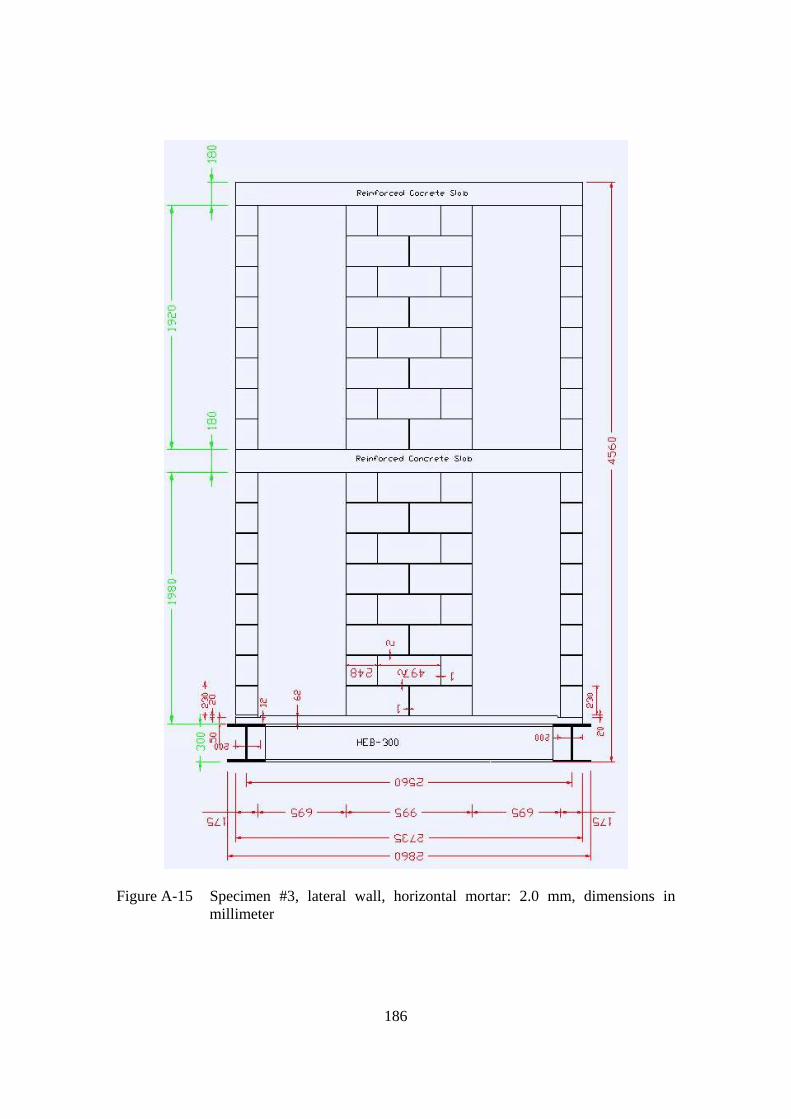
186

Figure A-15 Specimen #3, lateral wall, horizontal mortar: 2.0 mm, dimensions in

millimeter

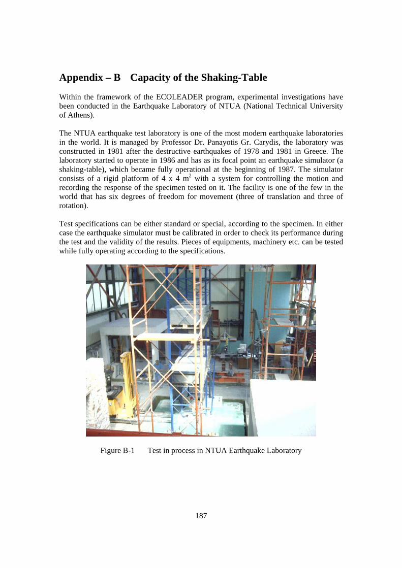
187

Appendix – B Capacity of the Shaking-Table Within the framework of the ECOLEADER program, experimental investigations have been conducted in the Earthquake Laboratory of NTUA (National Technical University of Athens). The NTUA earthquake test laboratory is one of the most modern earthquake laboratories in the world. It is managed by Professor Dr. Panayotis Gr. Carydis, the laboratory was constructed in 1981 after the destructive earthquakes of 1978 and 1981 in Greece. The laboratory started to operate in 1986 and has as its focal point an earthquake simulator (a shaking-table), which became fully operational at the beginning of 1987. The simulator consists of a rigid platform of 4 x 4 m2 with a system for controlling the motion and recording the response of the specimen tested on it. The facility is one of the few in the world that has six degrees of freedom for movement (three of translation and three of rotation). Test specifications can be either standard or special, according to the specimen. In either case the earthquake simulator must be calibrated in order to check its performance during the test and the validity of the results. Pieces of equipments, machinery etc. can be tested while fully operating according to the specifications.

Figure B-1 Test in process in NTUA Earthquake Laboratory

188

B-1 Main Activities in NTUA Laboratory The main activities in NTUA laboratory are:

• Earthquake resistance of buildings and civil engineering structures. Issue of seismic resistance certificates of urban units, structural systems, prefabricated buildings, building and substructures, seismic isolation systems, special structures (bridges), etc;

• Electrical, mechanical and electronic equipment which must operate normally in a vibration environment (control panels, computers, turbines, generators, switches, etc.);

• Vibration isolation systems for apparatuses and structures; • Vehicle suspension systems with simulation of road vibrations; • Regulations for the support of showcase exhibits or merchandise; • Calibration of vibration recording equipment; • Development and control of packaging systems for transportation and control of

packaging materials; • Testing of armament systems against strong vibrations.

Figure B-2 Static test facility and reaction wall behind it Characteristics of the Earthquake Simulator Platform – Mechanical Parts:

189

• Manufactured Country: USA, • Dimensions: 4 x 4 x 0.6 m3, • Weight: 10 to, • Material: Steel, • Number of independent degrees of freedom: six, • Maximum weight of specimen: 10 to, if center of mass is 2 m above the

simulator’s platform, • Maximum horizontal Force (directions, X, Y): 32 to, • Maximum vertical Force (direction Z): 64 to, • Maximum displacement of the platform (each axis):± 10 cm,

• Maximum rotation (about each axis): 2

7 10−

± ⋅ rad, • Maximum acceleration to each horizontal direction (X, Y): 1.5 g, • Maximum acceleration to vertical direction (Z): 2.9 g, • Maximum velocity to each axis (simultaneous performance): 89 cm / s, • Operating frequencies (for each degree of freedom): 0.1 – 100 Hz, • Electrical power installed: 1299 kVA.

B-2 Control Analog Unit A specific analog unit is installed to give the user the possibility of independent performance of each degree of freedom. The unit can produce and combine: sinusoidal, quadrangular etc. vibrations simultaneously. External recordings of other receivers can be used to provide input to the analogue unit. Digital Unit Mini computer PDP II/34 and its peripherals, possibility of exciting the platform with strong motion data stored in the computer, through D/A converter. The six degrees of freedom can be excited simultaneously or independently. Creation of input signals with specified source or other characteristics. B-3 Data Acquisition System Specific Unit with 64 channels Analog/Digital with high sweeping frequency, for the attendance of dynamic phenomena from several receivers (strain gauges, accelerometers, etc.). B-4 Storage of records (hard disks, tapes) Evaluation of input signals or specimen response records with the software libraries of the computer of the laboratory for earthquake engineering. Compensation of the error between desired and achieved input motion. The simulator is excited with a white noise signal produced with the available computer software and transfer-function ( )H ω of the specimen simulator system is estimated. The initial input signal is filtered with the reverse of the transfer-function 1( )H ω− in order to minimize the deviation between the desired and achieved input signal.

190

Appendix – C Specimens’ Specifications The experimental investigations included three specimens with various specifications as described in Table C-1:

Table C-1 Shaking-table test specimens (unreinforced-masonry) Name of the

specimen Number of

samples Type of sample Mortar in bed joints Mortar in head

joints

Specimen #1 1 without Gap-Element

normal (12 mm ) non–mortar

Specimen #2 1 Gap-Element (prototype)

normal (12 mm ) non–mortar

Specimen #3 1 Gap-Element thin-bed mortar 2 mm non–mortar C-1 Brick Units The brick units used for all of the specimens were of identical type. The brick size was 497 x 238 x 175 mm3, this is a typical kind of brick used in Germany by attention to thermal insulation and other parameters which are important for a country like Germany (see Figures C-1 and C-2). For all specimens, no mortar has been used in the head joints.

Figure C-1 Top view of brick unit used in all three specimens

191

Figure C-2 Brick’s boxes (6 x 7 = 42) Table C-2 shows properties of used bricks which are recommended by the producer company.

Table C-2 Properties of hollow clay brick recommended by the producer company

Name of the brick HLZ Mauerziegel Rohdichte 0.9 Format 12 DF Fire protection class F 120 – A Size (length, thickness, height), [mm] 497, 175, 238 Strength class 12 Characteristic strength [kN / m2] 11 Weight of each brick [kg] 17.6 Density [kg / m3] 900 Compression strength [MN / m2] 1.6-1.8

Table C-3 shows mechanical properties presented in Schubert results [13] (although some mechanical properties are given in Table C-2). Table C-3 Mechanical properties of used units, presented by Schubert test results,

(Brick Masonry HLz 12-0, 8-12 DF, Versuchsserie 4, Forschung F780) Average size: 492 x 172 x 241 mm3 Compression strength in vertical direction: 14.5 MPa (however with form factor 1.2 it is 17.4 MPa Compression strength in longitudinal direction: 2.8 MPa Tension strength in longitudinal direction without any compression force effect: 0.345 MPa Modulus of elasticity in longitudinal direction without any compression force effect: 2.4

192

GPa Tension strength in longitudinal direction with 0.5 σ * compression stress: 0.387 MPa Modulus of elasticity in longitudinal direction with 0.5 σ compression stress: 7.9 MPa Tension strength in longitudinal direction with 1σ compression stress: 0.373 MPa Modulus of elasticity in longitudinal direction with 1σ compression stress: 19.3 GPa Tension strength in vertical direction without any compression force effect: 0.77 MPa Modulus of elasticity in longitudinal direction without any compression force effect: 9 GPa Compression strength of the normal mortar (MG2a), with thickness 10 mm: 6 MPa Compression strength of the normal mortar (MG2a), with thickness 20 mm: 5.29 MPa Compression strength of brick and normal mortar: 5.58 MPa Shear modulus of elasticity of brick and normal mortar: 7 GPa Tension strength of brick and normal mortar: 0.20 MPa Shear modulus of elasticity of brick and normal mortar: 1.4 MPa *σ is the fundamental admissible compression stress according to DIN 1053-1, Table 4a and 4b C-2 Structural Specifications The first specimen should reflect the common way of constructing a masonry building. It was built with normal walls and normal mortar. Steel masses (5 to each) on top of the slabs have been used to model live loads. A part of the total live load has been provided by using an increased slab thickness (18 cm instead of 10 cm). Specimen #1 had two storeys with a total height of 4.40 m. All specimens had been constructed on top of a horizontal foundation frame made of structural steel. Thus, prefabrication of the specimens was possible without blocking time for other tests on the shaking-table. Figure C-3 shows one of the steel foundation frames.

Figure C-3 Removable steel foundation frame

193

All three specimens have similar roofs with the same dimensions and concrete materials. Dimensions of the roofs are 2710 x 2230 x 180 mm3 and ρ = 2400 kg / m3. Figure C-4 shows the constructing procedure of the roofs in NTUA laboratory.

Figure C-4 Roofs in constructing procedure After finishing of each storey, a prefabricated roof was pasted with a special type of glue on the walls. The steel masses for simulation of live loads and additional gravity were put on each storey in a symmetric position. To avoid slippery, they were fastened to the floor with long bolts. The first storey’s live load consisted of 200 pieces of steel in six rows with 980 x 330 x 10 mm3. On the second floor the mass consisted of only five big steel plates with symmetric distribution with dimension 1000 x 1000 x 130 mm3, Figure C-5 shows live loads and their positions on the first and second floor.

(a) (b)

Figure C-5 Live loads on first and second floor

194

In order to save time and material, the slabs elements of specimen #1 were also used for specimen #3. Transverse walls in the middle of the transverse sides were provided for lateral stability. Steel strips have been attached there in order to prevent an early out-of-plane failure of the transverse walls. To allow the deformation of the Corner-Gap-Element, no connection between the main walls and transverse walls has been provided.

Figure C-6 Steel strip in lateral walls for prevention of out-of-plane failure LVDT’s were installed for recording displacement in vertical, horizontal and diagonal directions of the main and lateral walls. Accelerometers only recorded horizontal acceleration of roofs in two horizontal directions. Figure C-7 shows instrument details of specimen #1.

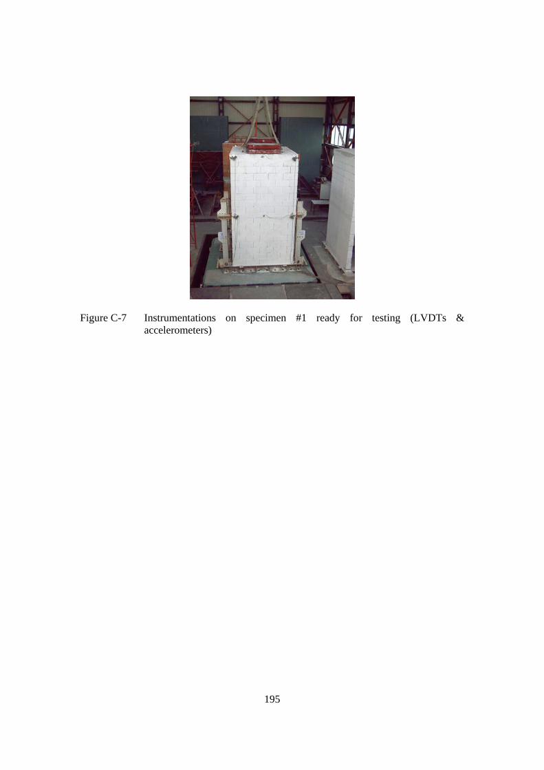
195

Figure C-7 Instrumentations on specimen #1 ready for testing (LVDTs &

accelerometers)

196

C-3 Engineering data of specimen #1 In the following the Table 5-4 shows engineering data of specimen #1.

Table C-4 Engineering data of specimen #1 Total weight (dead load + live load), [kg] 19,200 Number of storeys 2 Brick dimensions (length x height x thickness), [mm3] 497 x 238 x 175 Brick type / stiffness class HLZ / SFK 12 Mortar (thickness / type) 10-12 mm / IIa Live load in each storey, [to] 5 Roofs (concrete ρ = 2400 kg / m3) dimensions (l x h x t), [m3]

2.71 x 2.23 x 0.180

Height of the specimen, [m] 4.4 Number of table excitation time histories 11 Rate of excitation (table acceleration), [m / s2] 0.599 – 5.394 Structure fundamental period (before excitation), [s] 0.177

C-4 Engineering data of specimen #2 Specimen #2 as specified in Table C-1 is a specimen with Gap-Elements, but the other specifications are corresponding to the first one. The Gap-Element construction procedure is shown in Figure C-8:

(a) (b)

(c) (d)

Figure C-8 Gap-Element building procedure In order to allow a rocking movement of the base beam with the Corner-Gap-Elements, the middle reinforcement intentionally should not have any tensile connection to the steel

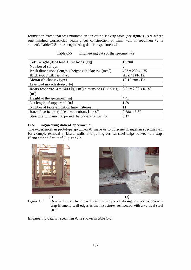
197

foundation frame that was mounted on top of the shaking-table (see figure C-8-d, where one finished Corner-Gap beam under construction of main wall in specimen #2 is shown). Table C-5 shows engineering data for specimen #2.

Table C-5 Engineering data of the specimen #2 Total weight (dead load + live load), [kg] 19,700 Number of storeys 2 Brick dimensions (length x height x thickness), [mm3] 497 x 238 x 175 Brick type / stiffness class HLZ / SFK 12 Mortar (thickness / type) 10-12 mm / IIa Live load in each storey, [to] 5 Roofs (concrete ρ = 2400 kg / m3) dimensions (l x h x t), [m3]

2.71 x 2.23 x 0.180

Height of the specimen, [m] 4.41 Net length of support b´, [m] 1.89 Number of table excitation time histories 11 Rate of excitation (table acceleration), [m / s2] 0.588 – 5.89 Structure fundamental period (before excitation), [s] 0.17

C-5 Engineering data of specimen #3 The experiences in prototype specimen #2 made us to do some changes in specimen #3, for example removal of lateral walls, and putting vertical steel strips between the Gap-Elements and first roof, Figure C-9.

(a) (b) Figure C-9 Removal of all lateral walls and new type of sliding stopper for Corner-

Gap-Element, wall edges in the first storey reinforced with a vertical steel strip

Engineering data for specimen #3 is shown in table C-6:

198

Table C-6 Engineering data of the specimen #3 Total weight (dead load + live load), [kg] 18,200 Number of storeys 2 Brick dimensions (length x height x thickness), [mm3] 497 x 238 x 175 Brick type / stiffness class HLZ / SFK 12 Mortar (thickness / type) , glue mortar 2 mm / DM Live load in each storey, [to] 5 Roofs (concrete ρ = 2400 kg / m3) dimensions (l x h x t), [m3]

2.71 x 2.23 x 0.180

Height of the specimen, [m] 4.26 Net length of support b´, [m] 1.89 Number of table excitation time histories 17 Rate of excitation (table acceleration), [m / s2] 0.542 – 12.03 Structure fundamental period (before excitation), [s] 0.152

199

Appendix – D Modified Spectrum for Specimen #3 During the test of specimen #3, the table excitation function has been changed. Allowable maximum table displacement is 100 mm as described in the table specifications. In order to avoid bumping of the table for high acceleration, table input data were changed, figure D-1 shows the comparison between maximum table acceleration vs. maximum table displacement for specimen #3.

0

20

40

60

80

100

120

0 2 4 6 8 10 12 14

Maximum Table Excitation (m/sec^2)

Max

imum

Tab

le D

ispl

acem

ent (

mm

)

Figure D-1 Maximum table horizontal displacement changed during excitation after

maximum table excitation 6.5 m / s2 Figures D-1 to D-7 depict the effects of the modifications to the response spectra.

200

Test 3-24 Acceleration Response Spectrum

0

5

10

15

20

25

30

0.5 2.5 4.5 6.5 8.5 10.5 12.5 14.5 16.5 18.5 20.5

Frequency (Hrz)

Sa (m

/sec

^2)

Damping = 0 %

Damping = 3 %

Damping = 5 %

Damping = 6 %

Damping = 7 %

Damping = 10 %

Figure D-2 Response spectra Sa for specimen #3, test 3-24

Test 3-26 Acceleration Response Spectrum

0

5

10

15

20

25

30

0.5 2.5 4.5 6.5 8.5 10.5 12.5 14.5 16.5 18.5 20.5

Frequency (Hrz)

Sa (m

/sec

^2)

Damping = 0 %

Damping = 3 %

Damping = 5 %

Damping = 6 %

Damping = 7 %

Damping = 10 %

Figure D-3 Response spectra Sa for specimen #3, test 3-26

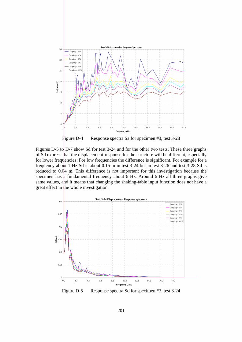
201

Test 3-28 Acceleration Response Spectrum

0

5

10

15

20

25

30

35

0.5 2.5 4.5 6.5 8.5 10.5 12.5 14.5 16.5 18.5 20.5

Frequency (Hrz)

Sa (m

/sec

^2)

Damping = 0 %

Damping = 3 %

Damping = 5 %

Damping = 6 %

Damping = 7 %

Damping = 10 %

Figure D-4 Response spectra Sa for specimen #3, test 3-28

Figures D-5 to D-7 show Sd for test 3-24 and for the other two tests. These three graphs of Sd express that the displacement-response for the structure will be different, especially for lower frequencies. For low frequencies the difference is significant. For example for a frequency about 1 Hz Sd is about 0.15 m in test 3-24 but in test 3-26 and test 3-28 Sd is reduced to 0.04 m. This difference is not important for this investigation because the specimen has a fundamental frequency about 6 Hz. Around 6 Hz all three graphs give same values, and it means that changing the shaking-table input function does not have a great effect in the whole investigation.

Test 3-24 Displacement Response spectrum

0

0.05

0.1

0.15

0.2

0.25

0.3

0.2 2.2 4.2 6.2 8.2 10.2 12.2 14.2 16.2 18.2

Frequency (Hrz)

Sd (m

)

Damping = 0 %

Damping = 3 %

Damping = 5 %

Damping = 6 %

Damping = 7 %

Damping = 10 %

Figure D-5 Response spectra Sd for specimen #3, test 3-24

202

Test 3-26 Displacement Response spectrum

0

0.01

0.02

0.03

0.04

0.05

0.06

0.07

0.2 2.2 4.2 6.2 8.2 10.2 12.2 14.2 16.2 18.2

Frequency (Hrz)

Sd (m

)

Damping = 0 %

Damping = 3 %

Damping = 5 %

Damping = 6 %

Damping = 7 %

Damping = 10 %

Figure D-6 Response spectra Sd for specimen #3, test 3-26

Test 3-28 Displacement Response spectrum

0

0.01

0.02

0.03

0.04

0.05

0.06

0.07

0.08

0.2 2.2 4.2 6.2 8.2 10.2 12.2 14.2 16.2 18.2

Frequency (Hrz)

Sd (m

)

Damping = 0 %

Damping = 3 %

Damping = 5 %

Damping = 6 %

Damping = 7 %

Damping = 10 %

Figure D-7 Response spectra Sd for specimen #3, test 3-28

203

Appendix – E Modified Graphs for Second Floor of Specimen #3

As it is explained in previous chapters, the vertical accelerations are generated by F.F.T. method. In this method the boundary points (approximately first/final twenty points of vertical accelerations) always were bigger than the expected values, for example see Figure E-23 or Figure E-25 (it is expected in start and finish of every dynamic test all of the dynamics responses of the structure oscillate near the zero and finally converge to the zero). For removing this small error from the calculations, all of the generated figures with even number in this appendix neglected those values.

Specimen #3, Second Floor Vertical Acceleration Test (10)

-5.0

-4.0

-3.0

-2.0

-1.0

0.0

1.0

2.0

3.0

4.0

5.0

0.0 0.5 1.0 1.5 2.0 2.5 3.0 3.5 4.0 4.5 5.0 5.5

Time [sec]

Acc

eler

atio

n [m

/s²]

Figure E-1 Vertical acceleration of second floor for test 3-10, specimen #3

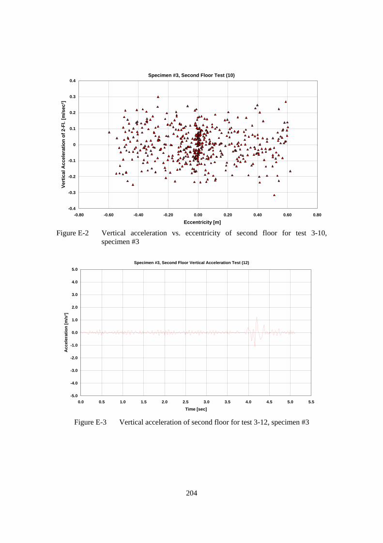
204

Specimen #3, Second Floor Test (10)

-0.4

-0.3

-0.2

-0.1

0

0.1

0.2

0.3

0.4

-0.80 -0.60 -0.40 -0.20 0.00 0.20 0.40 0.60 0.80

Eccentricity [m]

Vert

ical

Acc

eler

atio

n of

2-F

l. [m

/sec

²]

Figure E-2 Vertical acceleration vs. eccentricity of second floor for test 3-10,

specimen #3

Specimen #3, Second Floor Vertical Acceleration Test (12)

-5.0

-4.0

-3.0

-2.0

-1.0

0.0

1.0

2.0

3.0

4.0

5.0

0.0 0.5 1.0 1.5 2.0 2.5 3.0 3.5 4.0 4.5 5.0 5.5

Time [sec]

Acc

eler

atio

n [m

/s²]

Figure E-3 Vertical acceleration of second floor for test 3-12, specimen #3

205

Specimen #3, Second Floor Test (12)

-1.5

-1

-0.5

0

0.5

1

1.5

-1.00 -0.80 -0.60 -0.40 -0.20 0.00 0.20 0.40 0.60 0.80

Eccentricity [m]

Vert

ical

Acc

eler

atio

n of

2-F

l. [m

/sec

²]

Figure E-4 Vertical acceleration vs. eccentricity of second floor for test 3-12,

specimen #3

Specimen #3, Second Floor Vertical Acceleration Test (14)

-5.0

-4.0

-3.0

-2.0

-1.0

0.0

1.0

2.0

3.0

4.0

5.0

0.0 0.5 1.0 1.5 2.0 2.5 3.0 3.5 4.0 4.5 5.0 5.5

Time [sec]

Acc

eler

atio

n [m

/s²]

Figure E-5 Vertical acceleration of second floor for test 3-14, specimen #3

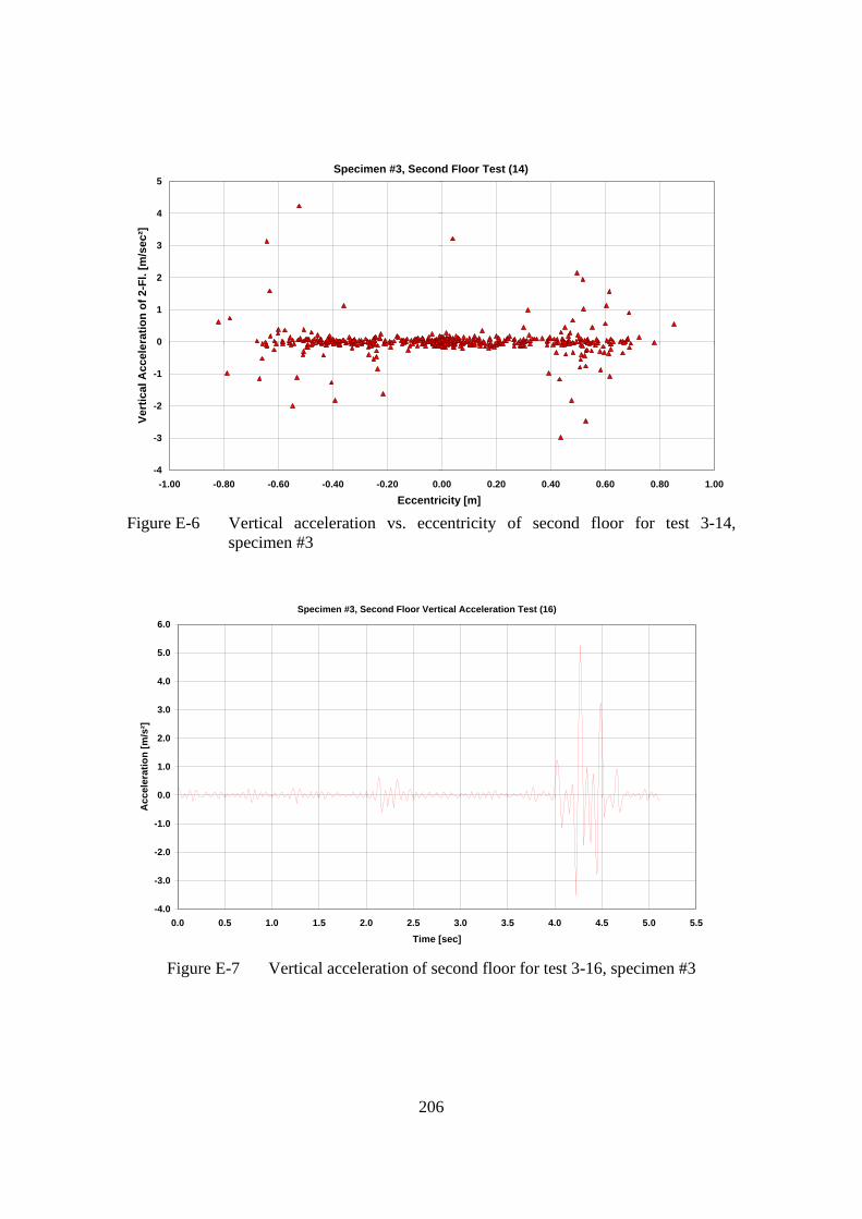
206

Specimen #3, Second Floor Test (14)

-4

-3

-2

-1

0

1

2

3

4

5

-1.00 -0.80 -0.60 -0.40 -0.20 0.00 0.20 0.40 0.60 0.80 1.00

Eccentricity [m]

Vert

ical

Acc

eler

atio

n of

2-F

l. [m

/sec

²]

Figure E-6 Vertical acceleration vs. eccentricity of second floor for test 3-14,

specimen #3

Specimen #3, Second Floor Vertical Acceleration Test (16)

-4.0

-3.0

-2.0

-1.0

0.0

1.0

2.0

3.0

4.0

5.0

6.0

0.0 0.5 1.0 1.5 2.0 2.5 3.0 3.5 4.0 4.5 5.0 5.5

Time [sec]

Acc

eler

atio

n [m

/s²]

Figure E-7 Vertical acceleration of second floor for test 3-16, specimen #3

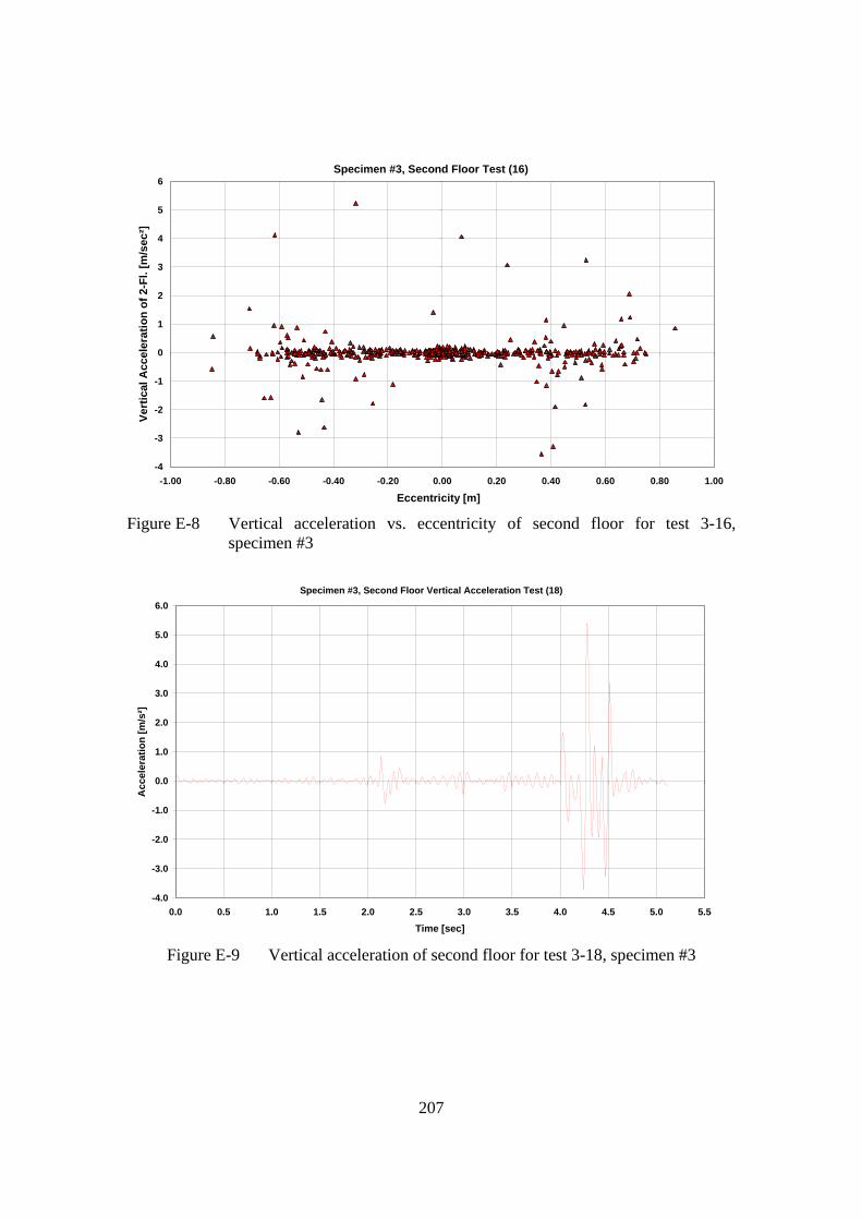
207

Specimen #3, Second Floor Test (16)

-4

-3

-2

-1

0

1

2

3

4

5

6

-1.00 -0.80 -0.60 -0.40 -0.20 0.00 0.20 0.40 0.60 0.80 1.00

Eccentricity [m]

Vert

ical

Acc

eler

atio

n of

2-F

l. [m

/sec

²]

Figure E-8 Vertical acceleration vs. eccentricity of second floor for test 3-16,

specimen #3

Specimen #3, Second Floor Vertical Acceleration Test (18)

-4.0

-3.0

-2.0

-1.0

0.0

1.0

2.0

3.0

4.0

5.0

6.0

0.0 0.5 1.0 1.5 2.0 2.5 3.0 3.5 4.0 4.5 5.0 5.5

Time [sec]

Acc

eler

atio

n [m

/s²]

Figure E-9 Vertical acceleration of second floor for test 3-18, specimen #3

208

Specimen #3, Second Floor Test (18)

-6

-4

-2

0

2

4

6

-1.00 -0.80 -0.60 -0.40 -0.20 0.00 0.20 0.40 0.60 0.80 1.00

Eccentricity [m]

Vert

ical

Acc

eler

atio

n of

2-F

l. [m

/sec

²]

Figure E-10 Vertical acceleration vs. eccentricity of second floor for test 3-18,

specimen #3

Specimen #3, Second Floor Vertical Acceleration Test (20)

-5.0

-4.0

-3.0

-2.0

-1.0

0.0

1.0

2.0

3.0

4.0

5.0

0.0 0.5 1.0 1.5 2.0 2.5 3.0 3.5 4.0 4.5 5.0 5.5

Time [sec]

Acc

eler

atio

n [m

/s²]

Figure E-11 Vertical acceleration of second floor for test 3-20, specimen #3

209

Specimen #3, Second Floor Test (20)

-4

-3

-2

-1

0

1

2

3

4

5

6

-1.00 -0.75 -0.50 -0.25 0.00 0.25 0.50 0.75 1.00

Eccentricity [m]

Vert

ical

Acc

eler

atio

n of

2-F

l. [m

/sec

²]

Figure E-12 Vertical acceleration vs. eccentricity of second floor for test 3-20,

specimen #3

Specimen #3, Second Floor Vertical Acceleration Test (22)

-5.0

-4.0

-3.0

-2.0

-1.0

0.0

1.0

2.0

3.0

4.0

5.0

0.0 0.5 1.0 1.5 2.0 2.5 3.0 3.5 4.0 4.5 5.0 5.5

Time [sec]

Acc

eler

atio

n [m

/s²]

Figure E-13 Vertical acceleration of second floor for test 3-22, specimen #3

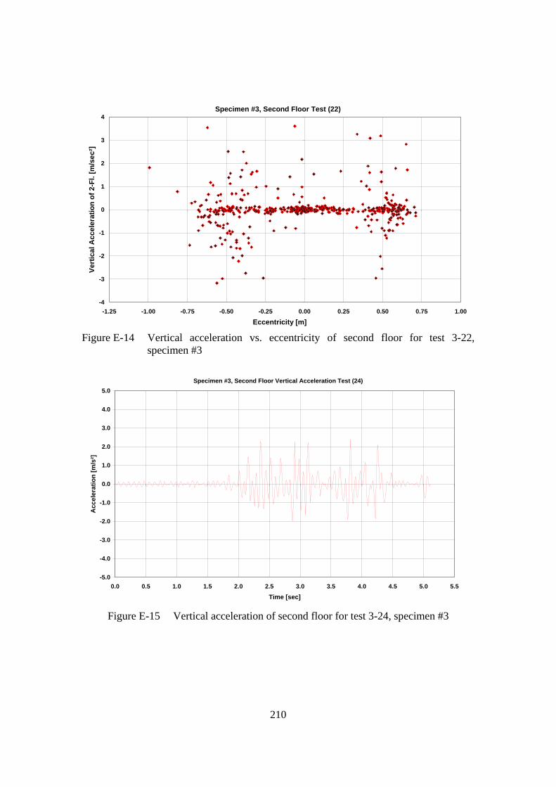
210

Specimen #3, Second Floor Test (22)

-4

-3

-2

-1

0

1

2

3

4

-1.25 -1.00 -0.75 -0.50 -0.25 0.00 0.25 0.50 0.75 1.00

Eccentricity [m]

Vert

ical

Acc

eler

atio

n of

2-F

l. [m

/sec

²]

Figure E-14 Vertical acceleration vs. eccentricity of second floor for test 3-22,

specimen #3

Specimen #3, Second Floor Vertical Acceleration Test (24)

-5.0

-4.0

-3.0

-2.0

-1.0

0.0

1.0

2.0

3.0

4.0

5.0

0.0 0.5 1.0 1.5 2.0 2.5 3.0 3.5 4.0 4.5 5.0 5.5

Time [sec]

Acc

eler

atio

n [m

/s²]

Figure E-15 Vertical acceleration of second floor for test 3-24, specimen #3

211

Specimen #3, Second Floor Test (24)

-2.5

-2

-1.5

-1

-0.5

0

0.5

1

1.5

2

2.5

3

-1.20 -1.00 -0.80 -0.60 -0.40 -0.20 0.00 0.20 0.40 0.60 0.80 1.00Eccentricity [m]

Vert

ical

Acc

eler

atio

n of

2-F

l. [m

/sec

²]

Figure E-16 Vertical acceleration vs. eccentricity of second floor for test 3-24,

specimen #3

Specimen #3, Second Floor Vertical Acceleration Test (26)

-5.0

-4.0

-3.0

-2.0

-1.0

0.0

1.0

2.0

3.0

4.0

5.0

0.0 0.5 1.0 1.5 2.0 2.5 3.0 3.5 4.0 4.5 5.0 5.5

Time [sec]

Acc

eler

atio

n [m

/s²]

Figure E-17 Vertical acceleration of second floor for test 3-26, specimen #3

212

Specimen #3, Second Floor Test (26)

-6

-4

-2

0

2

4

6

-1.00 -0.80 -0.60 -0.40 -0.20 0.00 0.20 0.40 0.60 0.80 1.00Eccentricity [m]

Vert

ical

Acc

eler

atio

n of

2-F

l. [m

/sec

²]

Figure E-18 Vertical acceleration vs. eccentricity of second floor for test 3-26,

specimen #3

Specimen #3, Second Floor Vertical Acceleration Test (28)

-6.0

-4.0

-2.0

0.0

2.0

4.0

6.0

0.0 0.5 1.0 1.5 2.0 2.5 3.0 3.5 4.0 4.5 5.0 5.5 6.0 6.5 7.0 7.5 8.0 8.5

Time [sec]

Acc

eler

atio

n [m

/s²]

Figure E-19 Vertical acceleration of second floor for test 3-28, specimen #3

213

Specimen #3, Second Floor Test (28)

-8

-6

-4

-2

0

2

4

6

8

-1.00 -0.80 -0.60 -0.40 -0.20 0.00 0.20 0.40 0.60 0.80 1.00Eccentricity [m]

Vert

ical

Acc

eler

atio

n of

2-F

l. [m

/sec

²]

Figure E-20 Vertical acceleration vs. eccentricity of second floor for test 3-28,

specimen #3

Specimen #3, Second Floor Vertical Acceleration Test (30)

-6.0

-4.0

-2.0

0.0

2.0

4.0

6.0

0.0 0.5 1.0 1.5 2.0 2.5 3.0 3.5 4.0 4.5 5.0 5.5 6.0 6.5 7.0 7.5 8.0 8.5

Time [sec]

Acc

eler

atio

n [m

/s²]

Figure E-21 Vertical acceleration of second floor for test 3-30, specimen #3

214

Specimen #3, Second Floor Test (30)

-6

-4

-2

0

2

4

6

-1.00 -0.75 -0.50 -0.25 0.00 0.25 0.50 0.75 1.00 1.25

Eccentricity [m]

Vert

ical

Acc

eler

atio

n of

2-F

l. [m

/sec

²]

Figure E-22 Vertical acceleration vs. eccentricity of second floor for test 3-30,

specimen #3

Specimen #3, Second Floor Vertical Acceleration Test (32)

-8.0

-6.0

-4.0

-2.0

0.0

2.0

4.0

6.0

8.0

10.0

0.0 0.5 1.0 1.5 2.0 2.5 3.0 3.5 4.0 4.5 5.0 5.5 6.0 6.5 7.0 7.5 8.0 8.5

Time [sec]

Acc

eler

atio

n [m

/s²]

Figure E-23 Vertical acceleration of second floor for test 3-32, specimen #3

215

Specimen #3, Second Floor Test (32)

-10

-8

-6

-4

-2

0

2

4

6

8

10

-1.20 -1.00 -0.80 -0.60 -0.40 -0.20 0.00 0.20 0.40 0.60 0.80Eccentricity [m]

Vert

ical

Acc

eler

atio

n of

2-F

l. [m

/sec

²]

Figure E-24 Vertical acceleration vs. eccentricity of second floor for test 3-32,

specimen #3

Specimen #3, Second Floor Vertical Acceleration Test (34)

-10.0

-8.0

-6.0

-4.0

-2.0

0.0

2.0

4.0

6.0

8.0

10.0

0.0 0.5 1.0 1.5 2.0 2.5 3.0 3.5 4.0 4.5 5.0 5.5 6.0 6.5 7.0 7.5 8.0 8.5

Time [sec]

Acc

eler

atio

n [m

/s²]

Figure E-25 Vertical acceleration of second floor for test 3-34, specimen #3

216

Specimen #3, Second Floor Test (34)

-6

-4

-2

0

2

4

6

8

-1.50 -1.25 -1.00 -0.75 -0.50 -0.25 0.00 0.25 0.50 0.75 1.00 1.25

Eccentricity [m]

Vert

ical

Acc

eler

atio

n of

2-F

l. [m

/sec

²]

Figure E-28 Vertical acceleration vs. eccentricity of second floor for test 3-34,

specimen #3