SEISMIC EVALUATION OF

EXISTING MULTI STOREY REINFORCED

CONCRETE BUILDING

by

Erol Kalkan

B.S. in C.E., Middle East Technical University, 1998

Submitted to the Institute for Graduate Studies in

Science and Engineering in partial fulfillment of

the requirements for the degree of

Master of Science

in

Civil Engineering

Boğaziçi University

2001

ii

SEISMIC EVALUATION OF

EXISTING MULTI STOREY REINFORCED

CONCRETE BUILDING

APPROVED BY :

Prof. Gülay Altay…………….………………………..…...

(Thesis Supervisor)

Prof. Turan Özturan…………..… ..……………………….

Assoc. Prof. Cavidan Yorgun……...…...………………….

DATE OF APPROVAL ……………………………..

iii

ACKNOWLEDGEMENTS

I would like to express my deepest gratitude to my supervisor Prof.Dr. Gülay

ALTAY for her support, guidance, tolerance and patience. I also grateful to Prof. Dr.

Haluk SUCUO LU for his help and support.

Sincere thanks are extended to Earthquake Research Center (METU/EERC) and

General Directorate of Disaster Affairs Earthquake Research Department for providing

necessary data and also their help.

iv

ABSTRACT

SEISMIC EVALUATION OF EXISTING MULTI STOREY

REINFORCED CONCRETE BUILDING

After 1998 Adana-Ceyhan Earthquake, many reinforced concrete buildings damaged

and some of them, which moderately damaged needed repairing and strengthening. In this

study, one of the moderately damaged six-storey building is selected and analyzed by

performing code static (elastic) analysis, code dynamic analysis and capacity spectrum

analysis after completing of seismic evaluation of the given structure, the states of the

building before and after strengthening are compared by performing inelastic static

analysis on three-dimensional model. In both states, the lateral load carrying capacity of

the frame system is determined by nonlinear static loading procedure called pushover

analysis. Then, the capacity of the structure is compared with earthquake demand in

Acceleration Displacement Response Spectra (ADRS) format by Capacity Spectrum

Method (CSM) and the performance of the structure is estimated.

The results of the analyses show that the applied static, dynamic and pushover

analysis are compatible with each other and rehabilitation procedure applied to the

moderately damaged structure in Adana city is satisfactorily effective in response to an

earthquake excitation. The added shearwalls increase the lateral stiffness and strength

considerably. The deformation capacity of structure is also improved.

v

ÖZET

ÇOK KATLI BETONARME YAPININ DEPREM

ANALİZİNİN YAPILMASI

1998 Adana-Ceyhan depreminden sonra bir çok betonarme yapı hasar gördü, bu

binalar arasında orta hasarlı olanların onarım ve güçlendirmeye ihtiyaçları vardı. Bu

çalı mada orta hasarlı altı katlı bir betonarme yapı örnek olarak alınmı ve elastik,

dinamik ve kapasite spektrumu analizleri ayrı ayrı uygulanarak, binanın sismik özellikleri

incelenmi tir. Binanın güçlendirme öncesi ve sonrası durumu, üç boyutlu modelleme

üzerinde elastik ötesi statik analiz yapılarak ayrıca incelenmi tir. Binanın her iki durumu

için çerçeve sisteminin yanal yük ta ıma kapasitesi statik itme analizi yöntemi ile elde

edilmi tir. Elde edilen kapasite eğrileri, Kapasite Spektrumu Metodu (CSM) kullanılarak

vme-Deformasyon Tepki Spektrumları (ADRS) formatında deprem spektrumu ile

kar ıla tırılmı ve yapının performansı belirlenmi tir.

Bu analizin sonuçları seçilen orta hasarlı binaya uygulanabilir onarım ve

güçlendirme yönteminin binanın deprem sırasındaki davranı ı açısından yeterli derecede

etkin olduğu sonucunu göstermi tir. Takviye amacıyla eklenen perde duvarlar binanın

yanal ötelenme kapasitesini ve rijitliğini önemli ölçüde artırmı tır. Takviye sonucunda

yapının deformasyon kapasitesi de artmı tır.

vi

To my wife, Narmina...

vii

TABLE OF CONTENTS

ACKNOWLEDGEMENT .......................................................…………………........ iii

ABSTRACT ........................................................................................…………….... iv

ÖZET ................................................................................................……………....... v

LIST OF TABLES ............................................................................……………....... x

LIST OF FIGURES ...........................................................................………………... xiii

LIST OF SYMBOLS ...........................................................................…………........ xvii

1. INTRODUCTION

1.1. General ...............................................................….……………………....… 1

1.2. Purpose .........…...........................................……………………......…......… 2

1.3. Object and Scope ..................................................………………………...… 2

1.4. Organization and Contents ...............................……………………..…….… 2

1.5. Uncertainty and Reliability .............................…………………………….… 3

1.6. Adana – Ceyhan Earthquake ..............….........……………………......…….. 3

1.6.1. Seismological Aspects ..............................……………………...….… 4

1.6.2 Geological Context .................................…………………………..… 5

1.6.3 Turkish Seismic Code and Adana Ceyhan Region ………………….. 6

1.7. Building Description .............………......................…………………...….… 7

1.7.1. Properties of Model Structure .........................…………………...…. 7

1.7.2. Properties of Cons. Materials Used in Structure …………………..... 7

2. MODELING OF STRUCTURE

2.1. General ........…………………………………..........………………...….…. 8

2.2. Building Considerations ……………..……....……………………….…….. 8

2.3. Element Models ……….........………………….….………………………... 9

2.3.1 Frame Elements ………...….………….…………………………..… 9

2.3.2 Slabs ……………..……...………..……….………………..……..… 11

3. LOADING CONDITIONS

3.1. General ……………..……...….………….……………………….…….….. 12

3.2. Dead Load Calculation ……………..……...…………………….…..…….. 12

3.3. Live Load Calculation ………….……….…….………………....………… 15

viii

4. CALCULATION OF MASS

4.1. General ……………..……...…………………...….……………………..… 17

4.2. Center of Mass ………………...……...….……….……………….….…… 18

4.3. Mass Moment of Inertia ……………..………...…...………………..…..…. 19

5. STATIC ANALYSIS

5.1. General ..............………….…….....................................…………………... 21

5.2. Definition of Elastic Seismic Loads ………….……...........………………... 21

5.3. Reduction of Elastic Seismic Loads .………….….............……….………... 26

5.4. Selection of Analysis Method ...........…..............…….………………...….. 27

5.5. Equivalent Seismic Load Method ....….................………………...……… 28

5.6. Analysis Procedure ……………………...…….……………………….…… 33

5.7. Defining of Irregularities in Plan ……….…….……………......................... 35

6. DYNAMIC ANALYSIS

6.1. General ..............……………….......................................………………...... 38

6.2. Eigenvector Analysis ……………….….…………………………………… 38

6.3. Modal Analysis Results …………….….…………………………………… 39

6.3.1. Periods and Frequencies ……….….……….…………………..…… 39

6.3.2. Participation Factors ………….….………………………….……… 41

6.3.3. Participating Mass Ratios …….….…………….…………………… 42

6.3.4. Total Unrestrained Mass and Location …….…..………………...… 43

6.4. Sufficient Number of Vibration Modes to be Considered ……….………… 44

6.5. Response – Spectrum Analysis …………………….……………..….….…. 45

6.5.1. Response – Spectrum Curve ……………………………...……….... 45

6.5.2. Modal Combination ………………..………….………...……..…… 46

6.6. Lower Limits of Response Quantities …………….…………….…..……… 48

6.7. Limitation of Storey Drifts ……………………….…………….…...……… 49

6.8. Second Order Effects ……………………………….………….…...……… 51

6.9. Dynamic Analysis Results …...……………….……………….…………... 52

7. CAPACITY SPECTRUM ANALYSIS

7.1. General ……………………………………..……………………….……… 57

7.2. Nonlinearity …………………….………........................………………....... 58

7.3. Capacity Spectrum Method ……………………….….…………………..… 59

7.3.1. Capacity Curve - Pushover ………….…..…………………..……… 59

ix

7.3.2. Demand Curve - Response Spectra ……….……………….…….… 61

7.3.3. Performance …………………….………………………….…….…. 61

7.4. Pushover Hinges ……..……………………………….………….……..… 62

7.5. Primary Ground Shaking Criteria .….……….........….…………....……… 65

7.5.1. Site Geology and Soil Characteristics ……......………………..…… 66

7.5.2. Site Seismicity Characteristics …...……….…………………..….... 66

7.5.3. Site Response Spectra …………………….……………………...… 68

7.6. Analysis Cases …………………….……...................….……………....… 69

7.7. Pushover Analysis Results ………………….….………………...……...... 73

7.8. Performance Evaluation with Capacity Spectrum Method ……...….…..… 77

7.9. Rehabilitation Scheme ………….......……....………..………….………... 80

7.10. Two Dimensional Pushover Analysis ..………….……….….…….…........ 85

7.11. Discussion of Results …………………......…….…………...…….…........ 86

8. SUMMARY, CONCLUSIONS AND RECOMMENDATIONS

8.1. Summary …….……………………...………………………...…………… 88

8.2. Conclusions …......................…………........….………………………........ 88

8.3. Future Recommendations .....…………………...………………….…........ 90

APPENDIX A. REHABILITATION OF MODERATELY DAMAGED R/C

BUILDING …...................................................................................... 91

REFERENCES …....................………….....................………………….………........ 95

REFERENCES NOT CITED .......................................………………….………........ 96

x

LIST OF TABLES

Table 3.1. Dimensions and amount of columns in the building …….………….....…... 13

Table 3.2. Dimensions and length of beams in the building …………...………..….… 13

Table 3.3. Dead load and live load values for each floor …..………………...……….. 16

Table 4.1. Calculated mass values for each floor ……..………………………...…….. 20

Table 5.1. Effective ground acceleration coefficient table …….…….………………... 22

Table 5.2. Building importance factor, table ………………….…….………….…...... 22

Table 5.3. Table of local site classes ……………….………….…..……………..….... 23

Table 5.4. Table of soil groups in EQ code ………………….………………...…...…. 24

Table 5.5. Table of local site classes corresponds to spectrum periods …….……...…. 24

Table 5.6. Table of building structural systems …………………………….…...……. 26

Table 5.7. Table of building types for selection of analysis …………..…………....…. 27

Table 5.8. Table of purpose occupancy of building ………….…….………….…...…. 30

Table 5.9. Total EQ load values for each floor ………………….....………….…….... 33

Table 5.10. Maximum drift differences between 1th and 2th floors ……..………..….... 36

Table 6.1. The distribution of periods with respect to mode numbers ….…………….. 40

xi

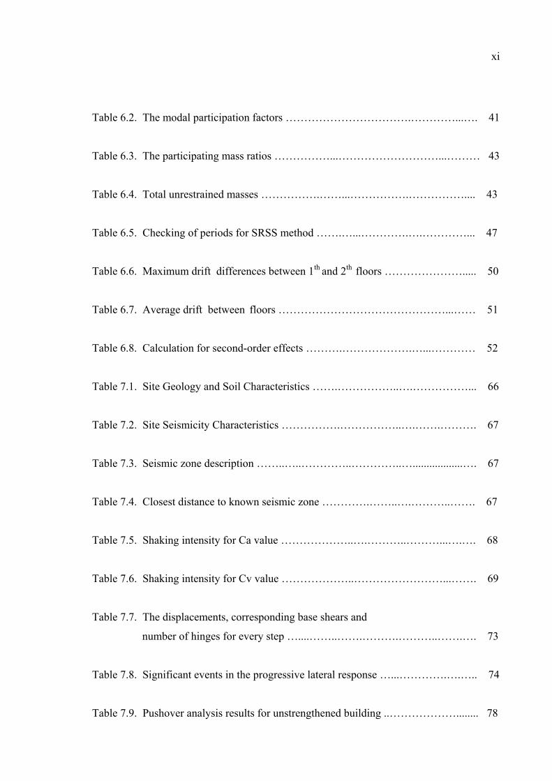
Table 6.2. The modal participation factors …………………………….…………...…. 41

Table 6.3. The participating mass ratios ……………...………………………...……… 43

Table 6.4. Total unrestrained masses …………….……...…………….…………….... 43

Table 6.5. Checking of periods for SRSS method …….…...………….….…………... 47

Table 6.6. Maximum drift differences between 1th and 2th floors …………………..... 50

Table 6.7. Average drift between floors ………………………………………...…… 51

Table 6.8. Calculation for second-order effects ……….……………….…...………… 52

Table 7.1. Site Geology and Soil Characteristics …….……………..….……………... 66

Table 7.2. Site Seismicity Characteristics …………….……………..….…….………. 67

Table 7.3. Seismic zone description ……..…..…………..…………..…..................…. 67

Table 7.4. Closest distance to known seismic zone ………….……..….………..……. 67

Table 7.5. Shaking intensity for Ca value ………………..….………..………...….…. 68

Table 7.6. Shaking intensity for Cv value ………………..……………………...……. 69

Table 7.7. The displacements, corresponding base shears and

number of hinges for every step …....……..…….……….………..…….…. 73

Table 7.8. Significant events in the progressive lateral response …...………….….….. 74

Table 7.9. Pushover analysis results for unstrengthened building ..………………........ 78

xii

Table 8.1. Shearwall ratio vs performance level comparison of the

assessed building ……………………..….………...….……………..……. 89

xiii

LIST OF FIGURES

Figure 1.1. Adana-Ceyhan region and epicenter of earthquake ……………………..…. 4

Figure 1.2. Acceleration Velocity and Disp. records of Adana-Ceyhan EQ………....… 5

Figure 1.3. Seismic hazard map of the Adana province ............................................….. 6

Figure 2.1. Shape of beam-column frame by using line elements …………….………. 10

Figure 2.2. 3D-Shape of building model …….…….…………………….……...…..…. 11

Figure 3.1. Illustration for net storey height ………………………..………….…….… 12

Figure 4.1. Mass moment of inertia about vertical axis ……………………………..… 18

Figure 4.2. Simplified floor plan for mass center determination ….……….……..…… 18

Figure 4.3. Simplified floor plan for MMI calculation …………….…………….…… 19

Figure 5.1. Special Design Acceleration Spectra ……………………………...………. 25

Figure 5.2. Special Design Acceleration Spectra for model structure ……………...…. 25

Figure 5.3. Special Design Acceleration Spectra for model structure ..……….………. 29

Figure 5.4. Total equivalent seismic load distribution to storey levels ……………..…. 32

Figure 5.5. Elastic Analysis, 3D deformed Shape …..………….………………...……. 34

Figure 5.6. Elastic Analysis, Top floor deformed Shape ………………….………...… 34

xiv

Figure 5.7. Shape of A1 type torsional irregularity …………………...……………… 35

Figure 6.1. The distribution of periods with respect to mode numbers ………………. 40

Figure 6.2. Special Design Acceleration Spectra for model structure…...……….…... 46

Figure 6.3. Mode 1, 3D Deformed Shape …………………………....………………. 52

Figure 6.4. Mode 1, Top floor deformed shape …...……………...…………………... 53

Figure 6.5. Mode 2, 3D Deformed Shape …………………….…………….….…….. 53

Figure 6.6. Mode 2, Top floor deformed shape …...………….…………………....… 54

Figure 6.7. Mode 3, 3D Deformed Shape …………………….…………….……..…. 54

Figure 6.8. Mode 3, Top floor deformed shape …...…………….………….…….…... 55

Figure 6.9. Mode Superposition , 3D Deformed Shape ……………………..…….… 55

Figure 6.10. Mode Superposition, Top floor deformed shape .…….………..……..….. 56

Figure 7.1. Concrete axial hinge …………..………....……………….……..……….. 63

Figure 7.2. Concrete shear hinge …..……..………....……………….……………….. 63

Figure 7.3. Concrete moment and PMM hinge ……....……………………....…….… 64

Figure 7.4. Details of used PMM and M3 hinge ..………………...……....……….…. 65

Figure 7.5. Typical force-deformation relationship for model element …………….… 74

xv

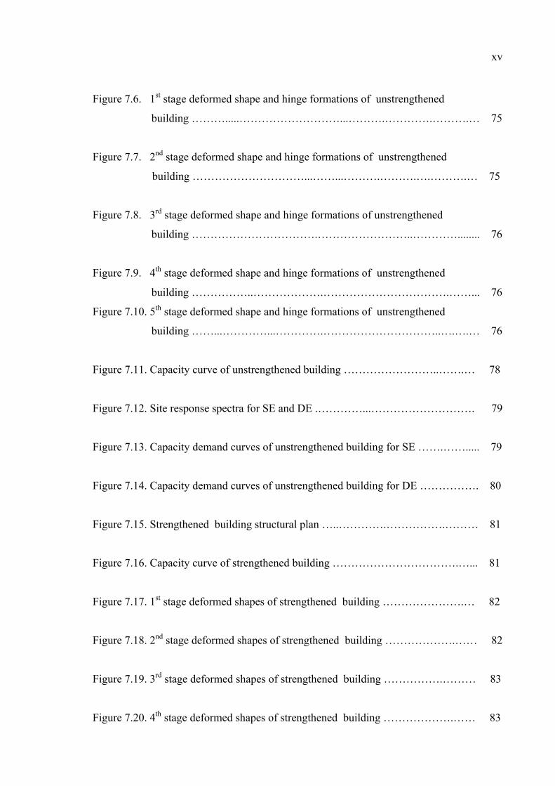
Figure 7.6. 1st stage deformed shape and hinge formations of unstrengthened

building ……….....………………………...……….………….……….… 75

Figure 7.7. 2nd stage deformed shape and hinge formations of unstrengthened

building …………………………...……...……….……….….……….… 75

Figure 7.8. 3rd stage deformed shape and hinge formations of unstrengthened

building …………………………….……………………..…………........ 76

Figure 7.9. 4th stage deformed shape and hinge formations of unstrengthened

building ……………..……………….…………………………….……... 76

Figure 7.10. 5th stage deformed shape and hinge formations of unstrengthened

building ……...…………...………….…………………………..….….… 76

Figure 7.11. Capacity curve of unstrengthened building ……………………..…….… 78

Figure 7.12. Site response spectra for SE and DE .…………...………………………. 79

Figure 7.13. Capacity demand curves of unstrengthened building for SE …….……..... 79

Figure 7.14. Capacity demand curves of unstrengthened building for DE ……………. 80

Figure 7.15. Strengthened building structural plan …..………….…………….……… 81

Figure 7.16. Capacity curve of strengthened building …………………………….…... 81

Figure 7.17. 1st stage deformed shapes of strengthened building ………………….… 82

Figure 7.18. 2nd stage deformed shapes of strengthened building ……………….…… 82

Figure 7.19. 3rd stage deformed shapes of strengthened building …………….……… 83

Figure 7.20. 4th stage deformed shapes of strengthened building ……………….…… 83

xvi

Figure 7.21. 5th stage deformed shapes of strengthened building ………………….… 83

Figure 7.22. Capacity demand curves of strengthened building for SE ……......…….... 85

Figure 7.23. Capacity demand curves of strengthened building for DE …..…………... 85

xvii

LIST OF SYMBOLS/ABBREVIATIONS

CA Shaking intensity (Acceleration)

CV Shaking intensity (Velocity)

NA Near source factor (Acceleration)

NV Near source factor (Velocity)

PF1φR1 Modal participation factors

Rx Ratio of displacements in x-direction

Ry Ratio of displacements in y-direction

Sa Spectral accelerations

Sd Spectral displacements

SD Soil profile

Tj Elastic period of vibration

V Base shear

W Weight of structure

Z Seismic zone factor

α1 Effective modal weight ratios

Δr Roof displacement

ADRS Acceleration displacement response spectrum

CQC Complete Quadratic Computation

CSM Capacity spectrum method

DE Design earthquake

DL Dead load

EQ Earthquake load

LL Live load

SE Serviceability earthquake

SRSS Squares of sum of squares

1

1. INTRODUCTION

1.1. General

Concrete is rather popular as a building material as well as in our country and almost

all over the world. For the most part, it serves its functions well; however concrete is

inherently brittle and performs poorly during earthquakes if not reinforced properly. The

last earthquakes dramatically showed this situation. 1997 code writers revised the design

provisions (Published in 1975) for new concrete buildings to provide adequate ductility to

resist strong ground shaking. There remain, nonetheless, millions of square meter of

nonductile concrete buildings in our country.

The consequences of neglecting this general risk are inevitably catastrophic for some

individual buildings. The collapse of single building has the potential for more loss of life

than any other catastrophe. The potential defects in these buildings are often not readily

apparent. This thesis is focused on the evaluation of these reinforced concrete buildings to

investigate their deficiencies during seismic shaking. Depending on the specific

characteristics of a particular building, one was selected from an array of alternatives.

Traditional design techniques assume that buildings respond elastically to

earthquakes. In reality, large earthquakes can severely damage buildings cause inelastic

behavior that dissipates energy. The assumption that buildings remain elastic simplifies the

engineer’s work but obscures a basic understanding of actual performance. The use of

traditional procedures for existing buildings can lead to erroneous conclusions on

deficiencies and unnecessarily high retrofit costs.

New analysis procedure described in this thesis, which is known as pushover analysis

describes the inelastic behavior of the structural members of a building better and this

technique can estimate more accurately the actual behavior of a building during a specific

ground motion. This analysis procedure tells how to identify which part of the building

will fail first.

2

1.2. Purpose

The primary purpose of this document is to provide the process of elastic and

inelastic analysis to an existing reinforced concrete building and to interpret the obtained

results. This thesis is intended to serve as an example reference for the future seismic

evaluations of reinforced concrete buildings.

1.3. Object and Scope

This thesis provides a comprehensive methodology and supporting commentary for

the seismic evaluation of existing concrete building. For this purpose, elastic analysis,

dynamic analysis and pushover analysis are used separately and obtained results are

compared in order to define the real behavior and damage zones of the structure under

earthquake excitation.

The existing building that had been selected as a model structure for this study is

located in Adana-Ceyhan region. It was a six-storey reinforced concrete residential

building, which was moderately damaged after Adana-Ceyhan Earthquake. The

architectural and structural plans of the building are given in Appendix Figures A.1 and

A.2.

1.4. Organization and Contents

This thesis is organized into 8 parts. Part 1 is the introductory part for the given

building, its site conditions and gives brief information about Adana-Ceyhan Earthquake.

Part 2 provides the guidelines, rules, and assumptions required to develop the analytical

model of buildings as three-dimensional system. In Part 3 and 4 load and mass calculations

are explained with details. Part 5 presents static analysis (Elastic Analysis) procedure. In

Part 6 dynamic analysis is carried out and results of this analysis are given. Part 7 presents

the generalized nonlinear static analysis procedure characterized by use of a static

pushover analysis method contains acceptability limits for the analysis results and Part 8

provides a detailed discussion of the various analysis results with the principal findings and

concluding remarks.

3

1.5. Uncertainty and Reliability

Uncertainty is a condition associated with essentially all aspects of earthquake

related science and engineering of the evaluation of existing buildings. The principle

sources of uncertainty lie in the characterization of seismic shaking, the determination of

materials properties of existing structural and geotechnical component capacities, and the

assignment of the acceptance limits on structural behavior. These uncertainties, for the

most part stemming from the lack of and / or the imperfect reliability of the specific

supporting data available, affect all analytical methods and procedures applied to the

challenge of seismic evaluation.

The performance-based methodology in other words Pushover Analysis presented in

this thesis cannot and does not eliminate these uncertainties. However through the use of

simplified static analysis and dynamic analysis, it provides a more sophisticated and direct

approach to address the uncertainties than do traditional linear analysis procedures. As a

result, this method is a useful and reliable design tool for assessment of expected building

behavior.

1.6. Adana-Ceyhan Earthquake

Adana-Ceyhan earthquake occurred on 27 June 1998 at 16:55 local time (13:55

GMT) having a magnitude mb = 5.9 resp. Mw = 6.3 shock southern Turkey [1].

The epicenter is located between the cities of Adana and Ceyhan about 30 km north

of the coast of the Mediterranean Sea, which is illustrated in Figure 1.1. The main fault,

which is in the northeast direction, can also be seen from this figure. The damage of the

reinforced concrete buildings in this Earthquake once again proved the low quality of the

reinforced concrete buildings in Turkey as it had happened in the Earthquakes of 1992

Erzincan, 1995 Dinar, 1999 Kocaeli and Düzce where great number of reinforced concrete

buildings had been damaged and collapsed.

In this earthquake about 150 people were killed, 1500 were injured and many

thousands were made homeless.

4

Figure 1.1. Adana-Ceyhan region and epicenter of earthquake [1]

Most of the observed damage occurred in traditional rural buildings, but many new

multi-story residential buildings and industrial buildings also suffered heavy damage or

even collapsed. The maximum intensity of the earthquake was estimated to read IX on the

EMS-scale.

1.6.1. Seismological Aspects

The earthquake parameters of the main shock on June 27, 1998 provided by the

Earthquake Research Department of Ankara (ERD) indicated a strike - slip earthquake

along a 65 degree SE dipping fault plane. The epicenter was located approximately 30 km

southeast of Adana at a depth of 23 km. A strong motion acceleration recording of the

main shock was made by ERD in the local branch building of the Agricultural Ministry in

5

Ceyhan located approximately 35 km from the epicenter. As shown in Figure 1.2 the peak

horizontal ground acceleration was 274 mg [1].

Figure 1.2. Acceleration Velocity and Displacement records of Adana-Ceyhan EQ [1]

1.6.2. Geological Context

The area of Adana city is characterized by a very large alluvial basin with a delta

shape, which extends more than 100 km east west and approximately 70 km north south.

Most of this basin is filled with quaternary recent Holocene deposits. In the southeast part

of the basin, some limestone formations from the Miocene, Oligocene and Eocene Ages

are visible at the surface. In the northern part of the basin, between Adana and Ceyhan,

outcrops of travertine formations are also visible [1].

1.6.3. Turkish Seismic Code and Adana-Ceyhan Region

6

The first official code for earthquake resistant design in Turkey, entitled

Specifications for Structures to be built in Disaster Areas, was published in 1975 (ERD

1975), according to this code Adana and Ceyhan were located in seismic zone 3, the

second highest five hazard zone (0 to 4), with a seismic zone coefficient Co = 0.08. Most of

the existing modern reinforced concrete buildings in Adana and Ceyhan areas were built

after 1975. It is unknown if the 1975 seismic code was systematically used in the design of

these buildings. The selected building for this thesis was also built after 1975 and in the

category of 1975 earthquake code [1].

In 1997, a new seismic code was introduced in Turkey (ERD 1997) and according to

this code the seismic hazard map of the Adana province is given in Figure 1.3 [1]. The

most part of the cities of Adana and Ceyhan are now situated in seismic zone II (Zone I is

the highest zone) however the selected building is located in seismic zone I.

Figure 1.3. Seismic hazard map of the Adana province [1]

1.7. Building Description

7

Brief information about the building that had been selected as a model structure for

this master thesis is given in the following subtopics:

1.7.1. Properties of Model Structure

Location : Adana-Ceyhan Region

Number of Storey : 6 Stories (having same storey height)

Storey Height : 3.00 m

Plan Dimensions : 20.15 x 14.25

Frame Type : Reinforced Concrete Elements (No any shear wall)

Usage Purpose : Residential

Seismic Zone : Zone 1 (According to Earthquake Code, 1998 )

Soil Type : Z3 (According to Earthquake Code, 1998)

Ductility Level : Enhanced

Slab Thickness : 15 cm

1.7.2. Properties of Construction Materials Used in Model Structure

Concrete : BS 20

Fck = 200 kgf/cm

Fcd = 137 kgf/cm

Ec = 25E6 KN/m

Steel : ST III

Fyd = 3650 kgf/cm

Partition Walls : Brick

d = 0.8 ton / m

8

2. MODELING OF STRUCTURE

2.1. General

Modeling rules represented in this part are intended to guide development of the

analytical model used to evaluate an existing building. Analytical building models based

on the following rules will be complete and accurate enough to support linear elastic

analysis, dynamic analysis and nonlinear static pushover analysis, described in Part 5,6 and

7. Analysis will usually rely on one or more specialized computer programs. Some

available programs can directly represent nonlinear load-deformation behavior of

individual components. Sap2000 is such a program by which the static, dynamic and

pushover analysis processes are carried out.

2.2. Building Considerations

Analytical models for evaluation must represent complete three-dimensional

characteristic of building behavior, including mass distribution, strength, stiffness and

deformability, through a full range of global and local displacements. SAP2000 Nonlinear

program enable us to obtain real behavior of structure by using three-dimensional

modeling.

The analytical model of the building should represent all new and existing

components that influence the mass, strength, stiffness, and deformability of the structure

at or near the expected performance point (Explained with details in Part 7). Elements and

components shown not to significantly influence the building assessment need not be

modeled.

Behavior of foundation components and effects of soil-structure interaction should

be modeled or shown to be insignificant to building assessment. The model of the

connection between the columns and foundation will depend on details of the column

foundation connection and the rigidity of the soil - foundation system.

9

According to the information taken from Middle East Technical University,

Earthquake Research Center (METU/EERC) about the given building, this structure has no

any problems coming from foundation and soil interaction. Therefore the end columns are

modeled as fixed supports at the base of the structure.

2.3. Element Models

An element is defined as either a vertical or a horizontal portion of a building that

acts to resist lateral and / or vertical load. Common vertical elements in reinforced concrete

construction include frames, shear walls and combined frame wall elements. Horizontal

elements commonly are reinforced concrete diaphragms. In the proceeding lines the

elements used in modeling of the given structure are described with details.

2.3.1. Frame Element

In the given structure, all vertical and lateral loads coming from slabs are transferred

to beams firstly then columns. Therefore the building can be modeled as a beam - column

frame type of structure.

The analysis model of a beam - column frame elements should represent the strength,

stiffness and deformation capacity of beams, columns, beam - column joints, and other

components that may be the part of the frame. Beam and column components should be

modeled considering flexural and shear rigidities, although the latter may be neglected in

many cases. Potential failure of anchorages and splices may require modeling of these

aspects as well. Rigid beam-column joints may be assumed.

The analytical model generally can represent a beam-column frame by using line

elements with properties concentrated at component centerlines (Given in Figure 2.1).

In some cases the beam and column centerlines will not coincide, in which case a

portion of the framing components may not be fully effective to resist lateral loads, and

component torsion may result. Where minor eccentricities occur (the centerline of the

10

narrower component falls within the middle third of the adjacent framing component

measured transverse to the framing direction), the effect of the eccentricity can be ignored.

Figure 2.1. Shape of beam-column frame by using line elements

Where larger eccentricities occur, the effect should be represented either by a

concentric frame model with reduced effective stiffness, strengths and deformation

capacities or by direct modeling of the eccentricity. Where transverse slabs or beams

connect beam and column component cross sections do not intersect, but instead beams

and columns, the transverse slabs or beams should be modeled directly.

In the modeling of the given structure, some beam and column centerlines do not

coincide, the effects of these minor eccentricities are not ignored and rigid link elements

are used.

Nonstructural components that interact importantly with the frame should be

modeled. Important nonstructural components that should be modeled include partial infill

(which may restrict the framing action of the columns) and full - height solid or perforated

infill and curtain walls (which may completely interrupt the flexural framing action of a

beam-column frame). In general, stairs need not be modeled.

11

A frame section is a set of material and geometric properties that describe the cross -

section of one or more frame elements. Sections are defined independently of the frame

elements, and are assigned to the elements. The main sections for beams in the structural

plan are 20x40 and 15x70 rectangular sections and the main sections for columns in the

structural plan are 60x25, 65x25, 75x25, 80x25, 60x30, 75x30, 40x30 and 85x25

rectangular sections. The unit for all sections is ‘cm’.

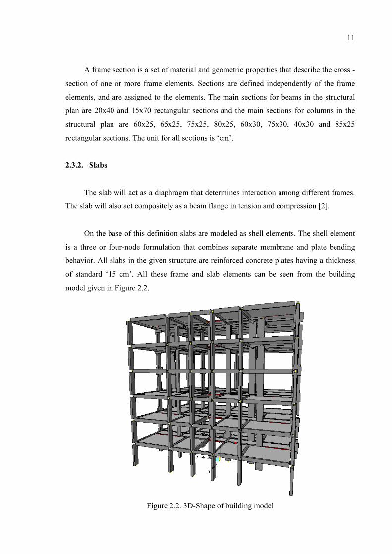
2.3.2. Slabs

The slab will act as a diaphragm that determines interaction among different frames.

The slab will also act compositely as a beam flange in tension and compression [2].

On the base of this definition slabs are modeled as shell elements. The shell element

is a three or four-node formulation that combines separate membrane and plate bending

behavior. All slabs in the given structure are reinforced concrete plates having a thickness

of standard ‘15 cm’. All these frame and slab elements can be seen from the building

model given in Figure 2.2.

Figure 2.2. 3D-Shape of building model

91

91

APPENDIX A : REHABILATED MODERATELY DAMAGED R/C

BUILDING

Figure A.1 is the architectural plan of the selecting building which has 6 storeys. By

using the architectural plan, the loading calculations are carried out. As it is observe, this

structure has no any soft storey condition.

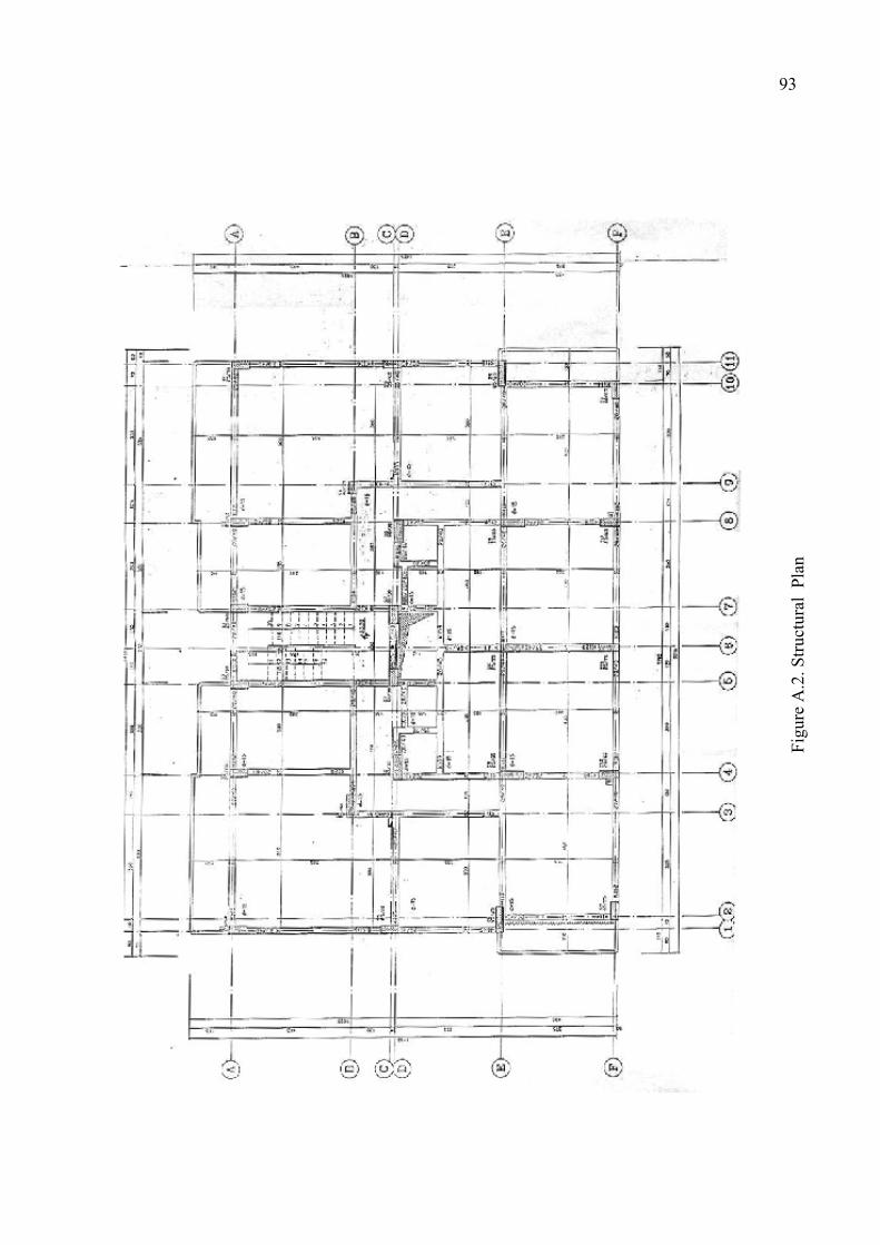
Figure A.2 shows the structural plan of the selecting building. By using the structural

plan, the modeling is done in Sap2000. As it is observe from the structural plan, this

structure has no any shear walls and some columns shows are distributed unsymetrically.

In Figure A.3, the modeling of the first storey is given. The numeration of joint can

be seen from this figure. Especially the location of control joint which is used in pushover

analysis can be seen form the figure

92

Figu

re A

.1. A

rchi

tect

ural

Pla

n

92

93

Figu

re A

.2. S

truct

ural

Pla

n

93

94

Figu

re A

.3. M

odel

ing

Plan

in S

AP2

000

94

12

3. LOADING CONDITIONS

3.1. General

The load calculation is carried out according to TS498 and Earthquake Code. On the

light of these references, if the given building plans are considered, it can be seen that this

structure has no any shear wall. The main structural elements on the plan for dead load

calculation are partition walls and reinforced concrete elements such as beams, columns

and slabs. This building is used as a residence therefore standard live load should also be

included. The calculations for both load cases are given in the following sub topics.

3.2. Dead Load Calculation

For the calculation of the total dead load, the weight of each structural member is

calculated separately. The details of weight calculations are as follows:

In order to define the dead load coming from the columns it is necessary firstly to

define the net storey height, for that purpose the slab thickness is subtracted from the

normal storey height. The storey height calculation is illustrated in Figure 3.1.

Height of Slab = 15 cm

Height of Storey = 300 cm Net Column Height = 285 cm

Figure 3.1. Illustration for net storey height

The dimensions and amount of columns in the building for any of the stories are

listed in Table 3.1, these values are taken from structural plan.

12

13

13

Table 3.1. Dimensions / amount of columns and weight calculations

AXES DIMENSIONS ( cm ) AMOUNT 60/25 4 F 65/25 1

85/25 2 E 80/25 2 75/25 1

25/60 2 D 60/30 4 75/30 1 B 40/30 1

A 25/60 4

TOTAL COLUMN AREA = 3.74 m TOTAL COLUMN VOLUME = ( 3.74 x 2.85 ) = 10.66 m .

WEIGHT OF COLUMNS = 10.66 m x 2.5 ton/m = 26.65 ton For i th floor

The dimensions and amounts of beams in the building for any of the floors is

given in Table 3.2.

Table 3.2. Dimensions of beams and weight calculations

AXIS DIMENSION ( cm ) LENGTH ( m ) A 40/20 17,70 B 40/20 7,40 40/20 17,20

D 15/70 4,60

E 40/20 16,70 F 40/20 16,70 TOTAL LENGTH 40/20 Beam = 140,60 m 1 40/20 7,90 15/70 Beam = 4,60 m 2 40/20 3,50 3 40/20 4,80 4 40/20 9,10 TOTAL VOLUME 5 40/20 5,00 140,60 x 0.40 x 0.20 = 11.3 m 6 40/20 4,30 4,60 x 0.70 x 0.15 = 0.5 m 7 40/20 5,00 8 40/20 9,10 TOTAL WEIGHT OF BEAMS 9 40/20 4,80 10 40/20 3,50 ( 11.3 + 0.5 ) x 2.5 = 30 ton For i th floor 11 40/20 7,90

14

14

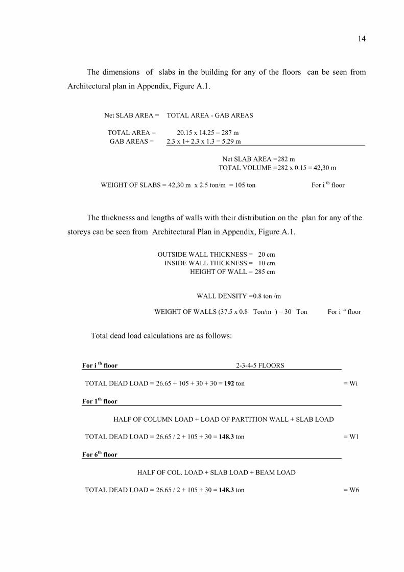
The dimensions of slabs in the building for any of the floors can be seen from

Architectural plan in Appendix, Figure A.1.

Net SLAB AREA = TOTAL AREA - GAB AREAS TOTAL AREA = 20.15 x 14.25 = 287 m GAB AREAS = 2.3 x 1+ 2.3 x 1.3 = 5.29 m Net SLAB AREA =282 m TOTAL VOLUME =282 x 0.15 = 42,30 m WEIGHT OF SLABS = 42,30 m x 2.5 ton/m = 105 ton For i th floor

The thicknesss and lengths of walls with their distribution on the plan for any of the

storeys can be seen from Architectural Plan in Appendix, Figure A.1.

OUTSIDE WALL THICKNESS = 20 cm INSIDE WALL THICKNESS = 10 cm HEIGHT OF WALL = 285 cm

WALL DENSITY =0.8 ton /m

WEIGHT OF WALLS (37.5 x 0.8 Ton/m ) = 30 Ton For i th floor

Total dead load calculations are as follows:

For i th floor 2-3-4-5 FLOORS TOTAL DEAD LOAD = 26.65 + 105 + 30 + 30 = 192 ton = Wi For 1th floor

HALF OF COLUMN LOAD + LOAD OF PARTITION WALL + SLAB LOAD TOTAL DEAD LOAD = 26.65 / 2 + 105 + 30 = 148.3 ton = W1 For 6th floor

HALF OF COL. LOAD + SLAB LOAD + BEAM LOAD TOTAL DEAD LOAD = 26.65 / 2 + 105 + 30 = 148.3 ton = W6

15

TOTAL DEAD LOAD OF FLOORS

W1 = 148,3 ton W2 = 192,0 ton W3 = 192,0 ton W4 = 192,0 ton W5 = 192,0 ton W6 = 148,3 ton

Weight : Kgf Length : cm Time : sec Mass : Ton

Metric unit system is used for the analysis part.

3.3. Live Load Calculation

The building is a residence therefore the corresponding live load value is taken from

TS 498 is equal to 200 kg/m .

The earthquake code states that live load values can be reduced by a specific amount.

This concept is explained with details in Part 5. Briefly here, reduction factor according to

5.4.3 is 0.3 for residential buildings and this reduction is taken into live load calculation as

follows:

15

qi = AREA x LL ( For Each Floor ) TOTAL FLOOR WEIGHTS ( ton ) qi = 282 m x 200 kg/m = 56.4 ton W1 = 165.2 ton W2 = 209.0 ton W1 = 148,3 + 0.3 x 56.4 = 165,2 ton For 1th floor W3 = 209.0 ton W4 = 209.0 ton Wi = 192 + 0.3 x 56.4 = 209 ton For ith floor W5 = 209.0 ton W6 = 148.3 ton W6 = 148,3 ton ( No LL on the roof ) For 6th floor

TOTAL LOAD OF BUILDING = 1149,5 ton

At the end of the load calculations the distribution of load values for each floor are

given in Table 3.3. These values are used in static and dynamic analysis, steps in Part 5 and

Part 6.

16

16

Table 3.3. Dead load and live load values for each floor

FLOOR DL LL 1 0,53 ton / m 0,2 ton / m 2 0,68 ton / m 0,2 ton / m 3 0,68 ton / m 0,2 ton / m 4 0,68 ton / m 0,2 ton / m 5 0,68 ton / m 0,2 ton / m 6 0,53 ton / m 0,0 ton / m

17

4. MASS CALCULATION

4.1. General

The mass of the structure is used to compute inertial forces in a dynamic analysis.

Normally, the mass is obtained from the elements using the mass density of the material

and the volume of the element.

For computational efficiency and solution accuracy, it is better to locate masses at

master joints. This means that there is no mass coupling between degrees of freedom at a

joint or between different joints. These uncoupled masses are always referred to the local

coordinate system of each joint. Mass values along restrained degrees of freedom are

ignored.

Inertial forces acting on the joints are related to the accelerations at the joints by a

6x6 matrix of mass values. These forces tend to oppose the accelerations. In a joint local

coordinate system, the inertia forces and moments F1, F2, F3, M1, M2 and M3 at a joint are

given by:

F1 u1 0 0 0 0 0 u1

F2 u2 0 0 0 0 u2

F3 u3 0 0 0 u3

M1 r1 0 0 r1

M2 r2 0 r2

M3 r3 r3

..

..

..

..

..

..=

Where u1, u2, u3, r1, r2, and r3 are the translation and rotation accelerations at the joint,

and the terms u1, u2, u3, r1, r2 and r3 are the specified mass values.

.... .... .. ..

Mass values must be given in consistent mass units ( W/g ) and mass moments of

inertia must be in WL /g units. Here W is weight, L is length, and g is the acceleration.

17

18

The used mass moment of inertia formula is given in Figure 4.1

Figure 4.1. Mass moment of inertia about vertical axis

Although Sap2000 calculates the masses and location of the master joints, mass

values are calculated in Part 3 and location of master joints are calculated below.

4.2. Center of Mass

The floor plan of the structure is almost symmetric with some exceptions about both

of X and Y axis. The plan view is divided into three parts for the calculation of the mass

center location (i.e. Master Joint Location). The simplified model for this purpose is used

and given in Figure 4.2.

18

Axis ‘C’

Mass Center

X

Y

33 cm

1 2 1

Figure 4.2. Simplified floor plan for mass center determination

19

19

M = Total mass of floor

M = m1 +m2 + m3 ( From Figure 4.2 )

m1 = 0.42 M m2 = 0.16 M m3 = 0.42 M

The mass center is found by taking the moment of inertia of simplified areas with respect

to the bottom line on Figure 4.3.

4.3. Mass Moment of Inertia

For the calculation of the mass moment of inertia, (4.1) is used; this formulation is

taken from Figure 4.1.

MMI = 1 / 12 ( b + h ) ( 4.1 )

MMI = Mass Moment of Inertia

b = Length one side in the X-direction in meters

h = Length one side in the Y-direction in meters

M = Total Mass in tons

d = Transferred Distance in meters

For the transformation of MMI in to another axis is calculated according to (4.2).

MMI = MMI + M x d ( 4.2 )

C1 d1 d1 O C2 d2 1 2 1

Figure 4.3. Simplified floor plan for MMI calculation

20

20

For Section -1- in Figure 4.3

MMI = 1/12 x (14.25 + 8.3 ) x M1

MMI = 22.61 M1

For Section -2- in Figure 4.3

MMI = 1/12 x (13 +2.5 ) x M2

MMI = 14.6 M2

For Section -3- in Figure 4.3

MMI = 1/12 x (14.25 + 8.3 ) x M3

MMI = 22.61 M3

After the each MMI of the three sections is transformed to the mass center axis, the total

mass moment of inertia is calculated as follows:

56.655 x M1 + 15.81 M2 + 56.655 x M3

M = M1 + M2 + M3

47.46 M + 2.53 M = 50 M

Here, M = Total mass of the floor.

The mass for each floor is calculated according to above formulation and listed in Table

4.1

Table 4.1. Calculated mass values for each floor

FLOOR TOTAL LOAD TOTAL MASS MMI

1 165,2 ton 16,84 ton/m.sec² 842,0 ton.m/sec² 2 209 ton 21,30 ton/m.sec² 1065,2 ton.m/sec² 3 209 ton 21,30 ton/m.sec² 1065,2 ton.m/sec² 4 209 ton 21,30 ton/m.sec² 1065,2 ton.m/sec² 5 209 ton 21,30 ton/m.sec² 1065,2 ton.m/sec² 6 148,3 ton 15,12 ton/m.sec² 755,9 ton.m/sec²

21

21

5. STATIC ANALYSIS

5.1. General

Static, dynamic and pushover analysis are used to determine the response of structure

to various loading cases. For static and dynamic loading cases, 1998 earthquake code is

used as a basic reference.

The static analysis of a structure involves the solution of the system of linear

equations represented by:

K u = r ( 5.1 )

Where K is the stiffness matrix, r is the vector of applied loads, and u is the vector of

resulting displacements [3].

For each defined load case, the analysis program automatically creates the load

vector r and solves the static displacements u.

In the first step of analysis, the seismic loads are calculated and in the next steps, on

the basis of earthquake code, static and dynamic loading are applied to the model structure

by using two methods which are described in the proceeding pages.

5.2. Definition of Elastic Seismic Loads

The Spectral Acceleration Coefficient, A(T), corresponding to 5% damped elastic

Design Acceleration Spectrum normalized by the acceleration of gravity, g, is given by

(5.2) which shall be considered as the basis for the determination of seismic loads [4].

A(T) = Ao I S(T) ( 5.2 )

22

22

The Effective Ground Acceleration Coefficient, Ao, appearing in (5.2) is specified in Table

5.1.

Table 5.1. Effective ground acceleration coefficient [4]

Seismic Zone Ao1 0.40 2 0.30 3 0.20 4 0.10

The model structure is located in Seismic Zone-1 (Refer to Part 1.7.1) , therefore the

corresponding effective ground acceleration Ao value is;

Ao = 0.40

The Building Importance Factor, I, appearing in (5.2) is specified in Table 5.2 [4].

Table 5.2. Building importance factor [4]

Purpose of Occupancy or Type of Building

Importance Factor ( I )

1. Buildings to be utilized after the earthquake and buildings containing hazardous materials a) Buildings required to be utilized immediately after the earthquake (Hospitals, dispensaries, health wards, fire fighting buildings and facilities, PTT and other telecommunication facilities, transportation stations and terminals, power generation and distribution facilities; governorate, county and municipality administration buildings, first aid and emergency planning stations) b) Buildings containing or storing toxic, explosive and flammable materials, etc.

1.5

2. Intensively and long-term occupied buildings and buildings preserving valuable goodsa) Schools, other educational buildings and facilities, dormitories and hostels, military barracks, prisons, etc. b) Museums

1.4

3. Intensively but short-term occupied buildings Sport facilities, cinema, theatre and concert halls, etc.

1.2

4. Other buildings Buildings other than above defined buildings. (Residential and office buildings, hotels, building-like industrial structures, etc.)

1.0

23

23

As it is stated in the introduction part, the model structure is used for residential purposes,

according to Table 5.2, the value of building importance factor is as follows;

I = 0.40

The Spectrum Coefficient, S(T), appearing in (5.2) shall be determined by Eqs.(5.3),

depending on the local site conditions and the building natural period, T (Fig. 5.1):

S(T) = 1 + 1.5 T / TA (0 T TA) ( 5.3a )

S(T) = 2.5 (TA < T TB) ( 5.3b )

S(T) = 2.5 (TB / T )0.8 (T > TB) ( 5.3c )

Spectrum Characteristic Periods, TA and TB , appearing in (5.3) are specified in

Table 5.5, depending on Local Site Classes given in Table 5.3 and Soil groups which is

given in Table 5.4.

As it is defined in Part 1.7.1 soil group for given structure is Group C and

corresponding local site class can be taken from Table 5.4.

Table 5.3. Table of local site classes [4]

Local Site Class

Soil Group according to Table 12.1 and Topmost Layer Thickness (h1)

Z1 Group (A) soils Group (B) soils with h1 15 m

Z2 Group (B) soils with h1 > 15 m

Group (C) soils with h1 15 m

Z3 Group (C) soils with 15 m < h1 50 m Group (D) soils with h1 10 m

Z4 Group (C) soils with h1 > 50 m

Group (D) soils with h1 > 10 m

According to Group C soil group and from the Table 5.3, the local site class of the given

structure is Z3.

24

24

Table 5.4. Table of soil groups in EQ code [4]

Soil

Group

Description of

Soil Group

Stand. Penetr.(N/30)

RelativeDensity

(%)

Unconf. Compres. Strength

(kPa)

Shear Wave

Velocity (m/s)

(A)

1. Massive volcanic rocks, unweathered sound metamorphic rocks, stiff cemented sedimentary rocks 2. Very dense sand, gravel... 3. Hard clay, silty lay……..

──

> 50 > 32

──

85─100 ──

> 1000 ──

> 400

> 1000 > 700 > 700

(B)

1. Soft volcanic rocks such as tuff and agglomerate, weathered cemented sedimentary rocks with planes of discontinuity…… 2. Dense sand, gravel.......... 3. Very stiff clay, silty clay..

──

30─50 16─32

──

65─85 ──

500─1000 ──

200─400

700─1000 400─700 300─700

(C)

1. Highly weathered soft metamorphic rocks and cemented sedimentary rocks with planes of discontinuity 2. Medium dense sand and gravel......…………………. 3. Stiff clay, silty clay..........

──

10─30 8─16

──

35─65 ──

< 500 ──

100─200

400─700

200─400 200─300

(D)

1. Soft, deep alluvial layers with high water table....…… 2. Loose sand.................….. 3. Soft clay, silty clay....…..

──

< 10 < 8

──

< 35 ──

── ──

< 100

< 200 < 200 < 200

Table 5.5. Table of local site classes corresponds to spectrum periods [4]

Local Site Class acc. to Table 12.2

TA(second)

TB(second)

Z1 0.10 0.30 Z2 0.15 0.40 Z3 0.15 0.60 Z4 0.20 0.90

Thus the corresponding spectrum periods from Table 5.5 in earthquake code are as

follows:

25

S(T)

2.5 S(T) = 2.5 (TB / T )0.8

1.0

T TA TBB

Figure 5.1. Special Design Acceleration Spectra

TA = 0.15 sec For Z3 type of soil.

TB = 0.60 sec

According to these periods, the obtained spectrum values are as follows:

S(T) = 1 + 1.5 T / TA (0 T 0.15)

S(T) = 2.5 (TA < T 0.60)

S(T) = 2.5 (TB / T )0.8 (T > 0.60)

With the light of these formulations, obtained ‘Special Design Acceleration Spectra ‘ is

given in Figure 5.2.

25

ACCELERATION SPECTRUM

0.00

0.50

1.00

1.50

2.00

2.50

3.00

0.0 0.5 1.0 1.5 2.0 2.

T ( sec )

PSA

/ g

( T )

5

Figure 5.2. Special Design Acceleration Spectra for model structure

26

26

When required, elastic acceleration spectrum may be determined through special

investigations by considering local seismic and site conditions. However spectral

acceleration coefficients corresponding to obtained acceleration spectrum ordinates shall in

no case be less than those determined by (5.2) based on relevant characteristic periods TA,

TB [4].

5.3. Reduction of Elastic Seismic Loads

Elastic seismic loads to be determined in terms of spectral acceleration coefficient

defined in equation A(T) = Ao I S(T) shall be divided to below defined Seismic Load

Reduction Factor to account for the specific nonlinear behavior of the structural system

during earthquake.

Seismic Load Reduction Factor, Ra(T), shall be determined by (5.4) here in terms of

Structural Behavior Factor, R, defined in Table 5.6 below for various structural systems,

and the natural vibration period T .

Ra(T) = 1.5 + (R 1.5) T / TA (0 T TA) (5.4a)

Ra(T) = R (T > TA) (5.4b)

Table 5.6. Table of building structural systems

BUILDING STRUCTURAL SYSTEM

Systems of Nominal Ductility

Level

Systems of High

Ductility Level

(1) CAST-IN-SITU REINFORCED CONCRETE BUILDINGS(1.1) Buildings in which seismic loads are fully resisted by frames................................................................................ (1.2) Buildings in which seismic loads are fully resisted by coupled structural walls...................................................... (1.3) Buildings in which seismic loads are fully resisted by solid structural walls........................................................... (1.4) Buildings in which seismic loads are jointly resisted by frames and solid and/or coupled structural walls............

4 4 4 4

8 7 6 7

27

The model structure has higher ductility level and all seismic loads are carried by

cast-in-situ reinforced concrete frames. Therefore the value of corresponding Structural

Reduction Factor is as follows;

R = 8 ( From Table 5.6 )

Ra(T) = 1.5 + 6.5T / 0.15 ( 0 T 0.15 sec )

Ra(T) = 8 ( T > 0.15 sec)

5.4. Selection of Analysis Method

Methods to be used for the seismic analysis of buildings and building-like structures

are, Equivalent Seismic Load Method given in 5.5, Mode-Superposition Method given in

6.5.

Buildings for which Equivalent Seismic Load Method given in 5.5 is applicable are

summarized in Table 5.7.

Table 5.7. Table of building types for selection of analysis

Seismic Total Height Zone Type of Building Limit

Buildings without type A1 torsional irregularity, or 1, 2 HN 25 m those satisfying the condition bi 2.0 at every storey Buildings without type A1 torsional irregularity, or

1, 2 those satisfying the condition bi 2.0 at every storey and at the same time without type B2 irregularity

HN 60 m

3, 4 All buildings HN 75 m

The model structure has a height of less than 25 m, located in the seismic zone of 1

although it has A1 type of irregularity and the constraints of bi 2.0 at every storey is

satisfied (Explained in Part 5.7). Therefore Equivalent Seismic Load Method can be safely

applied to the given structure.

27

28

28

5.5. Equivalent Seismic Load Method

Total Equivalent Seismic Load (Total Base Shear), Vt, acting on the entire building

in the earthquake direction considered shall be determined by (5.5) [4]. The model view for

total base shear is given in Figure 5.4.

Vt = W A(T1) / Ra(T1) 0.10 Ao I W ( 5.5 )

Here in (5.5) the first natural vibration period of the building, T1, shall be calculated

below. The first natural vibration period, which is permitted, is calculated by the

approximate method given here for buildings with HN 25 m in the first and second

seismic zones. This expression is given in (5.6) [4].

T1 T1A = Ct HN 3/4 ( 5.6 )

Since the height of the model structure is 18 m and less than 25 m, (5.6) is used for

the determination of the first natural period. Values of Ct in (5.6) are defined below

depending on the building structural system:

The value of Ct shall be calculated in (5.7) for buildings where seismic loads are fully

resisted by reinforced concrete structural walls [4].

Ct = 0.075 / At1/2 0.05 ( 5.7 )

Formulation of equivalent area At is given in (5.8) below where the maximum value

of ( wj/HN) shall be taken equal to 0.9 [4].

A = At wj [0.2 + ( wj / HN)2] ( 5.8 ) J

It shall be Ct = 0.07 for buildings whose structural system are composed only of

reinforced concrete frames or structural steel eccentric braced frames, Ct = 0.08 for

buildings made only of steel frames, Ct = 0.05 for all other buildings [4].

29

Since our system contains no any shear walls and structural system is only composed

of reinforced concrete frames the value of Ct is equal to 0.07.

Spectral acceleration coefficient formulation and seismic load reduction factor

formulations are given below according to (5.2) and (5.4)

A(T) = Ao I S(T) ( 5.2 )

Ao = 0.40

I = 1.0

S(T) = calculated acc. spectrum

A(T) = 0.40xS(T)

Ra(T) = 1.5 + 6.5T / 0.15 ( 0 T 0.15 sec ) ( 5.4a )

Ra(T) = 8 ( T > 0.15 sec) ( 5.4b )

Since T1 > 0.15 sec Ra(Tr) = 8

After defining Ct value the first natural period of the structure is calculated by (5.6)

then by using previously obtained acceleration spectra given in Figure 5.3, the

corresponding acceleration value to the first natural period is obtained.

ACCELERATION SPECTRUM

0,00

0,50

1,00

1,50

2,00

2,50

3,00

0,0 0,5 1,0 1,5 2,0 2,5

T ( sec )

PSA

/ g

( T )

29Figure 5.3. Special Design Acceleration Spectra for model structure

30

30

Total building weight, W, to be used in (5.5) shall be determined as follows;

T1 T1A = Ct HN ¾

HN 25 m and HN = 18 m

Ct = 0.07

T1 T1A = 0.611

S ( T ) = 2.46 According To Spectrum

A(T1) = Ao I S(T)

A(T1) = 0.984

N

W = wi ( 5.9 ) i = 1

Storey weights wi shall be calculated in 5.10

wi = gi + n qi ( 5.10 )

Live Load Participation Factor, n is given in Table 5.8

Table 5.8. Table of purpose occupancy of building

Purpose of Occupancy of Building N Depot, warehouse, etc. 0.80 School, dormitory, sport facility, cinema, theatre, concert hall, car park, restaurant, shop, etc.

0.60

Residence, office, hotel, hospital, etc. 0.30

Since the model structure is used for residential purposes the live load participation

factor is 0.3 according to Table 5.8 and the corresponding calculation is carried out as

follows;

31

Total equivalent seismic load determined by (5.5) is expressed in (5.11) as the sum of

equivalent seismic loads acting at storey levels.

qi = AREA x LL ( For Each Floor ) FLOOR WEIGHTS qi = 282 m² x 200 kg/m² = 56.4 ton W1 =165,2 ton W2 =209,0 ton W1 = 148,3 + 0.3 x 56.4 = 165,2 ton For 1th floor W3 =209,0 ton W4 =209,0 ton Wi = 192 + 0.3 x 56.4 = 209 ton For ith floor W5 =209,0 ton W6 =148,3 ton W6 = 148,3 ton ( No LL on the roof ) For 6th floor TOTAL LOAD OF BUILDING = 1150 ton

Vt = W A(T1) / Ra(T1) 0.10 Ao I W ( 5.5 )

N Vt = ΔFN + Fi ( 5.11 ) i = 1

Since HN < 25 m, additional equivalent seismic load, ΔFN, acting at the N’th storey (top)

of the building shall be taken as ΔFN = 0. Remaining part of the total equivalent seismic

load shall be distributed to stories of the building (including N’th storey) in accordance

with the equation given below (5.12).

wi Hi Fi = (Vt ΔFN) ────────── ( 5.12 ) N (wj Hj) j = 1

Vt = W A(T1) / Ra(T1) 0.10 Ao I W ( 5.5 )

W = 1150 ton ( Total Weight of Building Including LL) from 5.4.3

Vt = 1150 x 0.984 / 8 0.10 x 0.40 x 1.0 x 1150

Vt = 141.45 ton 46 ton OK

31

32

Total Equivalent Seismic Load calculations are carried out as follows;Total

Equivalent Seismic Load is distributed to storey levels as shown in Figure 5.4 by using the

(5.12) and the resultant values are tabulated in Table 5.9.

wi

Fi

w2 Hi

w1

Vt

Figure 5.4. Total equivalent seismic load distribution to storey levels

HN = 18 m < 25 m ΔFN = 0.0

wi Hi Fi = (141.45) ────────── ( 5.12 ) N

(wj Hj) j = 1

32

33

33

Table 5.9. Total EQ load values for each floor

FLOOR Wi ( ton ) H ( m ) Hi x Wi EQ LOAD ( ton ) 1 165,2 Ton 3,0 495,6 5,87 Ton 2 209 Ton 6,0 1254,0 14,85 ton 3 209 Ton 9,0 1881,0 22,28 ton 4 209 Ton 12,0 2508,0 29,70 ton 5 209 Ton 15,0 3135,0 37,13 Ton 6 148,3 Ton 18,0 2669,4 31,62 Ton

TOTAL 1150,0 Ton 11943,0 141,45 Ton

5.6. Analysis Procedure

The details of the modeling are explained in Part 2, dead loads and live loads are

applied to shell elements and earthquake loads which are tabulated in Table 5.9 are applied

to master joints of model. Load combination used in the analysis is as follows [5];

Load Combination = 1DL + 1LL + 1EQ

In the program stage this combination is called as ‘ COMB1 ‘, by using this load

combination static analysis is carried out, the deformed shapes of the static analysis are

given below in Figure 5.5and 5.6.

As it is given in deformed shapes, in X and Y directions lateral disturbance are

appearing. This is an expected result since structure seems symmetric however not purely

symmetric due to unsymmetrical distribution of the some columns.

34

Figure 5.5. Elastic Analysis, 3D deformed Shape

Figure 5.6. Elastic Analysis, Top floor deformed Shape

34

35

5.7. Defining of Irregularities in Plan

Since torsion seems critical due to asymmetry in the given building A1 type of

irregularity is checked below according to Earthquake Code requirements.

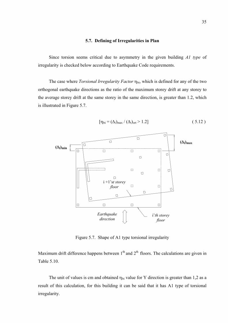
The case where Torsional Irregularity Factor bi, which is defined for any of the two

orthogonal earthquake directions as the ratio of the maximum storey drift at any storey to

the average storey drift at the same storey in the same direction, is greater than 1.2, which

is illustrated in Figure 5.7.

[ bi = (Δi)max / (Δi)ort > 1.2] ( 5.12 )

(Δi)max(Δi)min

i +1’st storeyfloor

Earthquakedirection

i’th storey floor

Figure 5.7. Shape of A1 type torsional irregularity

Maximum drift difference happens between 1th and 2th floors. The calculations are given in

Table 5.10.

The unit of values is cm and obtained bi value for Y direction is greater than 1,2 as a

result of this calculation, for this building it can be said that it has A1 type of torsional

irregularity.

35

36

36

Table 5.10. Maximum drift differences between 1th and 2th floors

JOINT UX UY JOINT UX UY DRIFT DIFF.X DRIFT DIFF.Y

1F1 0,4085 0,4785 2F1 1,1611 1,2858 0,7526 0,8073 1F2 0,4085 0,4321 2F2 1,1611 1,1663 0,7526 0,7342 1F3 0,4085 0,3916 2F3 1,1611 1,0618 0,7526 0,6702 1F4 0,4085 0,351 2F4 1,1611 0,9573 0,7526 0,6063 1F5 0,4085 0,3071 2F5 1,1611 0,8441 0,7526 0,5370 1F6 0,4448 0,4823 2F6 1,2544 1,2958 0,8096 0,8135 1F7 0,4448 0,4785 2F7 1,2544 1,2858 0,8096 0,8073 1F8 0,4448 0,4447 2F8 1,2544 1,1987 0,8096 0,7540 1F9 0,4448 0,4321 2F9 1,2544 1,1663 0,8096 0,7342 1F10 0,4448 0,3916 2F10 1,2544 1,0618 0,8096 0,6702 1F11 0,4448 0,3510 2F11 1,2544 0,9573 0,8096 0,6063 1F12 0,4448 0,3389 2F12 1,2544 0,9262 0,8096 0,5873 1F13 0,4448 0,3071 2F13 1,2544 0,8441 0,8096 0,5370 1F14 0,4448 0,3003 2F14 1,2544 0,8266 0,8096 0,5263 1F15 0,4650 0,4447 2F15 1,3067 1,1987 0,8417 0,7540 1F16 0,4650 0,4321 2F16 1,3067 1,1663 0,8417 0,7342 1F17 0,4650 0,4176 2F17 1,3067 1,1290 0,8417 0,7114 1F18 0,4650 0,4031 2F18 1,3067 1,0917 0,8417 0,6886 1F19 0,4650 0,3916 2F19 1,3067 1,0618 0,8417 0,6702 1F20 0,4650 0,3790 2F20 1,3067 1,0295 0,8417 0,6505 1F21 0,4650 0,3645 2F21 1,3067 0,9921 0,8417 0,6276 1F22 0,4650 0,3510 2F22 1,3067 0,9573 0,8417 0,6063 1F23 0,4650 0,3389 2F23 1,3067 0,9262 0,8417 0,5873 1F24 0,4766 0,4447 2F24 1,3366 1,1987 0,8600 0,7540 1F25 0,4766 0,4321 2F25 1,3366 1,1663 0,8600 0,7342 1F26 0,4766 0,4176 2F26 1,3366 1,1290 0,8600 0,7114 1F27 0,4766 0,4031 2F27 1,3366 1,0917 0,8600 0,6886 1F28 0,4766 0,3790 2F28 1,3366 1,0295 0,8600 0,6505 1F29 0,4766 0,3645 2F29 1,3366 0,9921 0,8600 0,6276 1F30 0,4766 0,3510 2F30 1,3366 0,9573 0,8600 0,6063 1F31 0,4766 0,3389 2F31 1,3366 0,9262 0,8600 0,5873 1F32 0,4790 0,4823 2F32 1,3428 1,2958 0,8638 0,8135 1F33 0,4790 0,4447 2F33 1,3428 1,1987 0,8638 0,7540 1F34 0,4790 0,4321 2F34 1,3428 1,1663 0,8638 0,7342 1F35 0,4790 0,4176 2F35 1,3428 1,1290 0,8638 0,7114 1F36 0,4790 0,4031 2F36 1,3428 1,0917 0,8638 0,6886 1F37 0,4790 0,3790 2F37 1,3428 1,0295 0,8638 0,6505 1F38 0,4790 0,3645 2F38 1,3428 0,9921 0,8638 0,6276 1F39 0,4790 0,3510 2F39 1,3428 0,9573 0,8638 0,6063 1F40 0,4790 0,3389 2F40 1,3428 0,9262 0,8638 0,5873 1F41 0,4790 0,3003 2F41 1,3428 0,8266 0,8638 0,5263 1F42 0,4805 0,4823 2F42 1,3465 1,2958 0,8660 0,8135 1F43 0,4805 0,4031 2F43 1,3465 1,0917 0,8660 0,6886 1F44 0,4805 0,3790 2F44 1,3465 1,0295 0,8660 0,6505 1F45 0,4805 0,3003 2F45 1,3465 0,8266 0,8660 0,5263

37

37

Table 5.10 Continued

1F46 0,4930 0,4823 2F46 1,3789 1,2958 0,8859 0,8135 1F47 0,4930 0,4447 2F47 1,3789 1,1987 0,8859 0,7540 1F48 0,4930 0,4321 2F48 1,3789 1,1663 0,8859 0,7342 1F49 0,4930 0,4031 2F49 1,3789 1,0917 0,8859 0,6886 1F50 0,4930 0,3790 2F50 1,3789 1,0295 0,8859 0,6505 1F51 0,4930 0,3510 2F51 1,3789 0,9573 0,8859 0,6063 1F52 0,4930 0,3389 2F52 1,3789 0,9262 0,8859 0,5873 1F53 0,4930 0,3003 2F53 1,3789 0,8266 0,8859 0,5263 1F54 0,5316 0,4823 2F54 1,4784 1,2958 0,9468 0,8135 1F55 0,5316 0,4321 2F55 1,4784 1,1663 0,9468 0,7342 1F56 0,5316 0,4031 2F56 1,4784 1,0917 0,9468 0,6886 1F57 0,5316 0,3790 2F57 1,4784 1,0295 0,9468 0,6505 1F58 0,5316 0,3510 2F58 1,4784 0,9573 0,9468 0,6063 1F59 0,5316 0,3003 2F59 1,4784 0,8266 0,9468 0,5263

Maximum Drift Difference in X direction = 0,9468 bi (-x-) = 1,110

Average Drift Difference in X direction = 0,8538

Maximum Drift Difference in Y direction = 0,8135 bi (-y-) = 1,217 Average Drift Difference in Y direction = 0,6702

38

38

6. DYNAMIC ANALYSIS

6.1. General

Dynamic analysis examines the behavior of the structure under dynamic loading

coming from ground excitation. In this part, 1998 earthquake code, which is known as

‘Specification for Structures to be Built in Disaster Areas’, is again used as a basic

reference besides other references.

The same model used in static analysis is taken into consideration for the dynamic

analysis with same dead load and live load values. These loads are applied to shell

elements. 12 modes are selected for the modal analysis and this number of modes is

checked in Part 6.4 to satisfy earthquake code requirements. The dynamic analysis applied

to given structure mainly including eigenvector analysis and response - spectrum analysis.

6.2. Eigenvector Analysis

Eigenvector analysis determines the undamped free-vibration mode shapes and

frequencies of the system. These natural modes provide an excellent insight into the

behavior of the structure.

Eigenvector analysis involves the solution of the generalized eigenvalue problem:

K M φ = 0 ( 6.1 )

where K is the stiffness matix, M is the diagonal mass matrix , is the diagonal matrix of

eigenvalues, and φ is the matrix of corresponding eigen vectors (ie. Mode Shapes).

Each eigenvalue - eigenvector pair is called a natural Vibration Mode of the

structure. The modes are identified by numbers from 1 to n in the order in which the modes

39

39

( 6.2 )f

T 1

are found.The eigenvalue is the square of the circular frequency , f , and period, T , of the

mode are related to by:

2f ( 6.3 )

The number of modes actually found, n, is limited by:

The number of mode requested, n

The number of mass degrees of freedom in the model

A mass degree of freedom is any active degree of freedom that possesses

translational mass or rotational mass moment of inertia. The mass may have been assigned

directly to the joint or may come from connected elements [2]. For the given structure

masses are applied to master joints, which are given with details in Part 4.

6.3. Modal Analysis Result

Various properties of the vibration modes can be obtained from dynamic analysis,

they are given in the following subtopics:

6.3.1. Periods and Frequencies

The following time - properties are given for each mode:

Period, T, in units of time

Cyclic frequency, f, in units of cycles per time (This is the inverse of ‘T’)

Circular frequency, w, in units of radians per time;

w = 2 f ( 6.4 )

40

At the end of the dynamic analysis, the following periods and frequencies

corresponding to 12 modes are obtained, and listed in Table 6.1. The distribution of

periods with respect to mode numbers is illustrated in Figure 6.1. As can be seen from both

these table and figure, the periods are decreasing regularly in a group of three. This is the

result of almost symmetrical distribution of the structural members in the building.

Although the 1st period of the structure seems high, this is the result of the non-existence of

the shear walls, weak lateral stiffness and asymmetric distribution of some columns on the

building. These low lateral stiffness in both X and Y-axis makes structure very weak

against lateral deformations.

Table 6.1. The distribution of periods with respect to mode numbers

MODE PERIOD FREQUENCY FREQUENCY EIGENVALUE (TIME) (CYC/TIME) (RAD/TIME) (RAD/TIME)2 1 0.909349 1.099687 6.909538 47.741722 2 0.786352 1.271696 7.990300 63.844889 3 0.761947 1.312427 8.246220 68.000141 4 0.280428 3.565979 22.405709 502.015783 5 0.241956 4.132990 25.968340 674.354657 6 0.236982 4.219721 26.513289 702.954511 7 0.149690 6.680452 41.974515 1761.860 8 0.128251 7.797194 48.991216 2400.139 9 0.126857 7.882905 49.529753 2453.196 10 0.095690 10.450390 65.661738 4311.464 11 0.081514 12.267833 77.081070 5941.491 12 0.080241 12.462452 78.303896 6131.500

PERIOD VS MODE

0

2

4

6

8

10

12

14

0,00 0,20 0,40 0,60 0,80 1,00 1,20

PERIOD ( sec )

MO

DE

NU

MB

ER

40Figure 6.1. The distribution of periods with respect to mode numbers

41

6.3.2. Participation Factors

The model participation factors are the dot products of the three acceleration loads

with the mod shapes. The participation factors for mode ’n’ corresponding to acceleration

loads in the global X, Y, and Z directions are given by:

( 6.5 )

xTnxn mf

( 6.6 ) y

Tnyn mf

( 6.7 ) z

Tnzn mf

Where n is the mode shape and mx, my and mz are the unit acceleration loads. These

factors are the generalized loads acting on the mode due to each of the acceleration loads.

They are referred to the global coordinate system. These values are called ‘ factors ‘

because they are related to the mode shape and to unit acceleration. The mode shapes are

each normalized, or scaled, with respect to the mass matrix such that:

nT M n = 1 ( 6.8 )

The actual magnitudes and signs of the participation factors are not important. What

important is the relative values of three factors for a given mode. The modal participation

factors obtained from dynamic analysis are listed in Table 6.2.

Table 6.2. The modal participation factors

MODE PERIOD UX UY UZ

1 0.909349 -0.885425 0.021743 .000000 2 0.786352 -0.020077 -0.981984 .000000 3 0.761947 0.417258 -0.000562 .000000 4 0.280428 0.300008 -0.007031 .000000 5 0.241956 -0.007680 -0.344394 .000000 6 0.236982 -0.171041 0.003595 .000000 7 0.149690 -0.169182 0.003777 .000000 8 0.128251 0.009098 0.207287 .000000 9 0.126857 -0.128562 0.010155 .000000 10 0.095690 0.110632 -0.002760 .000000 11 0.081514 -0.008476 -0.151222 .000000

41 12 0.080241 -0.110436 0.009226 .000000

42

6.3.3. Participating Mass Ratios

The participation mass ratio for a mode provides a measure of how important the

mode is for computing the response to the acceleration loads in each of three global

directions. The participation mass ratios for mode n corresponding to acceleration loads in

the global X, Y, and Z direction are given by:

x

xnxn M

fP2)( ( 6.9 )

y

ynyn M

fP

2)( ( 6.10 )

z

znzn M

fP2)(

( 6.11 )

Where fxn, fyn, and fzn are the participation factors defined in the previous

subtopic; and Mx, My, and Mz are the total unrestrained masses acting in the X, Y, and Z

directions. The participating mass ratios are expressed as percentages.

The cumulative sums of the participating mass ratios for all modes up to mode ‘n’

can be obtained separately. This measure of how many modes are required to achieve a

given level of accuracy for ground acceleration, the requirements for this accuracy is

explained in Part 6.4.

If all eigen - modes of the structure are present, the participating mass ratio for each

of the three acceleration loads should generally be 100%. However, this may not be the

case in the presence of certain types of constraints where symmetry conditions prevent

some of the mass from responding to translational accelerations. The participating mass

ratios obtained from dynamic analysis are given in Table 6.3.

42

43

43

Table 6.3. The participating mass ratios

MODE PERIOD INDIVIDUAL MODE (PERCENT) CUMULATIVE SUM (PERCENT) UX UY UZ UX UY UZ 1 0.909349 66.8694 0.0403 0.0000 66.8694 0.0403 0.0000 2 0.786352 0.0344 82.2494 0.0000 66.9038 82.2898 0.0000 3 0.761947 14.8502 0.0000 0.0000 81.7540 82.2898 0.0000 4 0.280428 7.6770 0.0042 0.0000 89.4310 82.2940 0.0000 5 0.241956 0.0050 10.1166 0.0000 89.4360 92.4106 0.0000 6 0.236982 2.4953 0.0011 0.0000 91.9313 92.4117 0.0000 7 0.149690 2.4414 0.0012 0.0000 94.3727 92.4129 0.0000 8 0.128251 0.0071 3.6649 0.0000 94.3798 96.0779 0.0000 9 0.126857 1.4098 0.0088 0.0000 95.7895 96.0867 0.0000 10 0.095690 1.0440 0.0006 0.0000 96.8335 96.0873 0.0000 11 0.081514 0.0061 1.9505 0.0000 96.8396 98.0378 0.0000 12 0.080241 1.0403 0.0073 0.0000 97.8799 98.0451 0.0000

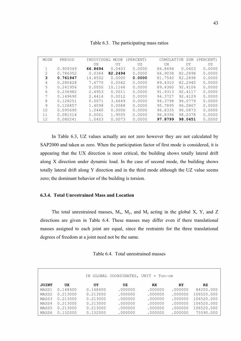
In Table 6.3, UZ values actually are not zero however they are not calculated by

SAP2000 and taken as zero. When the participation factor of first mode is considered, it is

appearing that the UX direction is most critical, the building shows totally lateral drift

along X direction under dynamic load. In the case of second mode, the building shows

totally lateral drift along Y direction and in the third mode although the UZ value seems

zero; the dominant behavior of the building is torsion.

6.3.4. Total Unrestrained Mass and Location

The total unrestrained masses, Mx, My, and Mz acting in the global X, Y, and Z

directions are given in Table 6.4. These masses may differ even if there translational

masses assigned to each joint are equal, since the restraints for the three translational

degrees of freedom at a joint need not be the same.

Table 6.4. Total unrestrained masses

IN GLOBAL COORDINATES, UNIT = Ton-cm JOINT UX UY UZ RX RY RZ MASS1 0.168400 0.168400 .000000 .000000 .000000 84200.000 MASS2 0.213000 0.213000 .000000 .000000 .000000 106520.000 MASS3 0.213000 0.213000 .000000 .000000 .000000 106520.000 MASS4 0.213000 0.213000 .000000 .000000 .000000 106520.000 MASS5 0.213000 0.213000 .000000 .000000 .000000 106520.000 MASS6 0.152000 0.152000 .000000 .000000 .000000 75590.000

44

44

6.4. Sufficient Number of Vibration Modes To Be Considered

Sufficient number of vibration modes, n, to be taken into account in the analysis shall

be determined to the criterion that the sum of effective participating masses calculated for

each mode in each of the given X and Y lateral earthquake directions perpendicular to each

other shall in no case be less than 90% of the total building mass. In the earthquake

direction considered, all vibration modes with effective participating masses exceeding 5%

of the total building mass shall also be taken into account [2].

n n N N Mxr = [ (mi xir)]2 / Mr 0.90 mi (6.12a) r = 1 r = 1 i = 1 i = 1 n n N N M = [ (myr i yir)]2 / Mr 0.90 mi (6.12b) r = 1 r = 1 i = 1 i = 1

The expression of Mr appearing in Eqs.(6.12) is given below for buildings where

floors behave as rigid diaphragms:

N Mr = (mi xir

2 + mi yir2 + m i ir

2) (6.13) i = 1

Eqs.(6.12) and (6.13) are used by SAP2000 and the obtained participating ratios are

listed in Table 6.3. As can be seen from Table 6.3. The 12 mode number gives almost 98%

of mass participating value and this percentage is satisfies the earthquake code

requirements where the limit value for the number of modes in the case of mass

participating ratios is given as 90%.

In this method, maximum internal forces and displacements are determined by the

statistical combination of maximum contributions obtained from each of the sufficient

number of natural vibration modes considered [4].

45

6.5. Response - Spectrum Analysis

The dynamic equilibrium equations associated with the response of a structure to

ground motion are given in (6.14).

K u(t) + C u(t) + M u(t) = mx ugx (t) + my ugy (t) + mzugz(t) ( 6.14 ) ... .. .. ..

Where K is the stiffness matrix; C is the proportional damping matrix; M is the

diagonal mass matrix; u, u, and u are the relative displacements, velocities, and

accelerations with respect to the ground; mx, my, and mz are the unit acceleration loads; and

ugx, ugy, and ugz are the components of uniform ground acceleration.

...

.. .. ..

Response - spectrum analysis seeks the likely maximum response to these equations

rather than the full time history. The earthquake ground acceleration in each direction is

given as a digitized response - spectrum curve of pseudo - spectral acceleration response

versus period of structure.

Even though accelerations may be specified in three directions, only a single,

positive result is produced for each quantity. The response quantities include

displacements, forces, and stresses. Each computed result represents a statistical measure

of the likely maximum magnitude for that response quantity. The actual response can be

expected to vary within a range from this positive value to its negative.

No correspondence between two different response quantities is available. No

information is available as to when this extreme value occurs during the seismic loading,

or as to what the values of other response quantities are at that time.

6.5.1. Response - Spectrum Curve

The response - spectrum curve for a given direction is defined by digitized points of

pseudo - spectral acceleration response versus period of the structure. This curve chosen

45

46

46

should reflect the damping that is present in the structure being modeled. The used

response spectrum curve, which has a 5% damping, is given in Figure 6.2.

ACCELERATION SPECTRUM

0,00

0,50

1,00

1,50

2,00

2,50

3,00

0,0 0,5 1,0 1,5 2,0 2,5

T ( sec )

PSA

/ g

( T )

Figure 6.2. Special Design Acceleration Spectra for model structure

6.5.2. Modal Combination

For a given direction of acceleration, the maximum displacements, forces, and

stresses are computed throughout the structure for each of the vibration modes. These

modal values for a given response quantity are combined to produce a single, positive

result for the given direction of acceleration. Rules to be applied for the statistical

combination of non-simultaneous maximum contributions of response quantities calculated

for each vibration mode, such as the base shear, storey shear, internal force components,

displacement and storey drift, are specified in the following provided that they are applied

independently for each response quantity:

6.5.2.1. SRSS Method

This method is used in order to combine the modal results by taking the sum of their

absolute values .In the cases where natural periods of any two vibration mode with Ts < Tr

always satisfy the condition Ts / Tr < 0.80, Square Root of Sum of Squares (SRSS) Rule

may be applied [4].

47

The SRSS method is checked in Table 6.5 according to earthquake code requirement

and as a result, the period ratios are not satisfying 0.80 value, therefore SRSS method is

not suitable for superimposing of mode values for the given model.

Table 6.5. Checking of periods for SRSS method

MODE PERIOD (sec) Ts / Tr 1 0,909349 2 0,786352 0,86 3 0,761947 0,97 4 0,280428 0,37 5 0,241956 0,86 6 0,236982 0,98 7 0,14969 0,63 8 0,128251 0,86 9 0,126857 0,99

10 0,09569 0,75 11 0,081514 0,85 12 0,080241 0,98

Ts / Tr < 0.80

6.5.2.2. CQC Method

Complete Quadratic Combination (CQC) technique described by Wilson, Der

Kiureghian and Bayo (1981) is the default method of modal combination.

The CQC method takes into account the statistical coupling between closely spaced

modes caused by modal damping. Increasing the modal damping increases the coupling

between closely spaced modes. If the damping is zero for all modes, this method

degenerates to the SRSS method.

In the cases where the requirements above for the SRSS method for the given

condition are not satisfied, Complete Quadratic Combination (CQC) Rule shall be applied

for the combination of maximum modal contributions.

Since SRSS method is not satisfying the requirement of the Earthquake Code for the

given building, Complete Quadratic Combination (CQC) Rule is used for the superposition

47

48

48

of the modes. In the application of this rule, modal damping factors shall be taken as 5%

for all modes.

6.6. Lower Limits of Response Quantities

In the case where the ratio of the base shear in the given earthquake direction, VtB,

which is obtained through modal combination according to Part 6.5, to the base shear, Vt,

obtained by Equivalent Seismic Load Method through 5.4 is less than the below given

value of (VtB < Vt), all internal force and displacement quantities determined by Mode

Superposition Method shall be amplified in accordance with (6.14) [4].

BD = ( Vt / VtB) BB ( 6.14 )

In the case where at least one of the irregularities of type A1, B2 or B3 exists in a

building =1.00, whereas none of them exists =0.90 shall be used in (6.14).

=1.0 for our model due to A1 Type of Irregularity according to Part 5.7 therefore;

VtB < Vt ( 6.15 )

VtB = 141.46 ton. Obtained from modal combination, this base shear value is

calculated according to support reaction.

Vt = 141.45 ton. Obtained from Equivalent Seismic Load Method, the details of

calculations are given in Table 5.9.

According to (6.15);

VtB < Vt

141.46 1x141.45

Therefore the requirement of Earthquake Code given in Part 6.6 is satisfied

49

49

6.7. Limitation of Storey Drifts

The storey drift, Δi, of any column or structural wall shall be determined by (6.16) as

the difference of displacements between the two consecutive stories.

Δi = di di 1 ( 6.16 )

In (6.16) di and di 1 represent lateral displacements obtained from the analysis at

the ends of any column or structural wall at stories i and i-1.

The maximum value of storey drifts within a storey, (Δi)max , calculated by (6.16) for

columns and structural walls of the ith storey of a building for each earthquake direction

shall satisfy the unfavorable one of the conditions given by (6.17) and (6.18).

(Δi)max / hi 0.0035 ( 6.17 )

(Δi)max / hi 0.02 / R ( 6.18 )

R = 8 According to Part 5.3.1 then

(Δi)max / hi 0.02 / R = 0.0025

In the cases where the conditions specified by (6.17) and (6.18) are not satisfied at

any storey, the earthquake analysis shall be repeated by increasing the stiffness of the

structural system.

The maximum drift difference happens between 1th and 2th floors. The calculations

for the limitation of the storey drift are given in Table 6.6.

hi = 300 cm according to Part 1.7.1 then

As a result of Table 6.6, the conditions specified by (6.17) and (6.18) are satisfied at

any storey in the given building.

50

50

Table 6.6. Maximum drift differences between 1th and 2th floors

JOINT ux uy JOINT ux uy Δi x Δi y Δi x / h i Δi y / h i

1F1 0,4085 0,4785 2F1 1,1611 1,2858 0,7526 0,8073 0,0025 0,0027 1F2 0,4085 0,4321 2F2 1,1611 1,1663 0,7526 0,7342 0,0025 0,0024 1F3 0,4085 0,3916 2F3 1,1611 1,0618 0,7526 0,6702 0,0025 0,0022 1F4 0,4085 0,351 2F4 1,1611 0,9573 0,7526 0,6063 0,0025 0,0020 1F5 0,4085 0,3071 2F5 1,1611 0,8441 0,7526 0,5370 0,0025 0,0018 1F6 0,4448 0,4823 2F6 1,2544 1,2958 0,8096 0,8135 0,0027 0,0027 1F7 0,4448 0,4785 2F7 1,2544 1,2858 0,8096 0,8073 0,0027 0,0027 1F8 0,4448 0,4447 2F8 1,2544 1,1987 0,8096 0,7540 0,0027 0,0025 1F9 0,4448 0,4321 2F9 1,2544 1,1663 0,8096 0,7342 0,0027 0,0024

1F10 0,4448 0,3916 2F10 1,2544 1,0618 0,8096 0,6702 0,0027 0,0022 1F11 0,4448 0,3510 2F11 1,2544 0,9573 0,8096 0,6063 0,0027 0,0020 1F12 0,4448 0,3389 2F12 1,2544 0,9262 0,8096 0,5873 0,0027 0,0020 1F13 0,4448 0,3071 2F13 1,2544 0,8441 0,8096 0,5370 0,0027 0,0018 1F14 0,4448 0,3003 2F14 1,2544 0,8266 0,8096 0,5263 0,0027 0,0018 1F15 0,4650 0,4447 2F15 1,3067 1,1987 0,8417 0,7540 0,0028 0,0025 1F16 0,4650 0,4321 2F16 1,3067 1,1663 0,8417 0,7342 0,0028 0,0024 1F17 0,4650 0,4176 2F17 1,3067 1,1290 0,8417 0,7114 0,0028 0,0024 1F18 0,4650 0,4031 2F18 1,3067 1,0917 0,8417 0,6886 0,0028 0,0023 1F19 0,4650 0,3916 2F19 1,3067 1,0618 0,8417 0,6702 0,0028 0,0022 1F20 0,4650 0,3790 2F20 1,3067 1,0295 0,8417 0,6505 0,0028 0,0022 1F21 0,4650 0,3645 2F21 1,3067 0,9921 0,8417 0,6276 0,0028 0,0021 1F22 0,4650 0,3510 2F22 1,3067 0,9573 0,8417 0,6063 0,0028 0,0020 1F23 0,4650 0,3389 2F23 1,3067 0,9262 0,8417 0,5873 0,0028 0,0020 1F24 0,4766 0,4447 2F24 1,3366 1,1987 0,8600 0,7540 0,0029 0,0025 1F25 0,4766 0,4321 2F25 1,3366 1,1663 0,8600 0,7342 0,0029 0,0024 1F26 0,4766 0,4176 2F26 1,3366 1,1290 0,8600 0,7114 0,0029 0,0024 1F27 0,4766 0,4031 2F27 1,3366 1,0917 0,8600 0,6886 0,0029 0,0023 1F28 0,4766 0,3790 2F28 1,3366 1,0295 0,8600 0,6505 0,0029 0,0022 1F29 0,4766 0,3645 2F29 1,3366 0,9921 0,8600 0,6276 0,0029 0,0021 1F30 0,4766 0,3510 2F30 1,3366 0,9573 0,8600 0,6063 0,0029 0,0020 1F31 0,4766 0,3389 2F31 1,3366 0,9262 0,8600 0,5873 0,0029 0,0020 1F32 0,4790 0,4823 2F32 1,3428 1,2958 0,8638 0,8135 0,0029 0,0027 1F33 0,4790 0,4447 2F33 1,3428 1,1987 0,8638 0,7540 0,0029 0,0025 1F34 0,4790 0,4321 2F34 1,3428 1,1663 0,8638 0,7342 0,0029 0,0024 1F35 0,4790 0,4176 2F35 1,3428 1,1290 0,8638 0,7114 0,0029 0,0024 1F36 0,4790 0,4031 2F36 1,3428 1,0917 0,8638 0,6886 0,0029 0,0023 1F37 0,4790 0,3790 2F37 1,3428 1,0295 0,8638 0,6505 0,0029 0,0022 1F38 0,4790 0,3645 2F38 1,3428 0,9921 0,8638 0,6276 0,0029 0,0021 1F39 0,4790 0,3510 2F39 1,3428 0,9573 0,8638 0,6063 0,0029 0,0020 1F40 0,4790 0,3389 2F40 1,3428 0,9262 0,8638 0,5873 0,0029 0,0020 1F41 0,4790 0,3003 2F41 1,3428 0,8266 0,8638 0,5263 0,0029 0,0018 1F42 0,4805 0,4823 2F42 1,3465 1,2958 0,8660 0,8135 0,0029 0,0027 1F43 0,4805 0,4031 2F43 1,3465 1,0917 0,8660 0,6886 0,0029 0,0023 1F44 0,4805 0,3790 2F44 1,3465 1,0295 0,8660 0,6505 0,0029 0,0022 1F45 0,4805 0,3003 2F45 1,3465 0,8266 0,8660 0,5263 0,0029 0,0018

51

51

Table 6.6. Continued

1F46 0,4930 0,4823 2F46 1,3789 1,2958 0,8859 0,8135 0,0030 0,0027 1F47 0,4930 0,4447 2F47 1,3789 1,1987 0,8859 0,7540 0,0030 0,0025 1F48 0,4930 0,4321 2F48 1,3789 1,1663 0,8859 0,7342 0,0030 0,0024 1F49 0,4930 0,4031 2F49 1,3789 1,0917 0,8859 0,6886 0,0030 0,0023 1F50 0,4930 0,3790 2F50 1,3789 1,0295 0,8859 0,6505 0,0030 0,0022 1F51 0,4930 0,3510 2F51 1,3789 0,9573 0,8859 0,6063 0,0030 0,0020 1F52 0,4930 0,3389 2F52 1,3789 0,9262 0,8859 0,5873 0,0030 0,0020 1F53 0,4930 0,3003 2F53 1,3789 0,8266 0,8859 0,5263 0,0030 0,0018 1F54 0,5316 0,4823 2F54 1,4784 1,2958 0,9468 0,8135 0,0032 0,0027 1F55 0,5316 0,4321 2F55 1,4784 1,1663 0,9468 0,7342 0,0032 0,0024 1F56 0,5316 0,4031 2F56 1,4784 1,0917 0,9468 0,6886 0,0032 0,0023 1F57 0,5316 0,3790 2F57 1,4784 1,0295 0,9468 0,6505 0,0032 0,0022 1F58 0,5316 0,3510 2F58 1,4784 0,9573 0,9468 0,6063 0,0032 0,0020 1F59 0,5316 0,3003 2F59 1,4784 0,8266 0,9468 0,5263 0,0032 0,0018

6.8. Second - Order Effects

In the case where Second-Order Effect Indicator, i, satisfies the condition given by

(6.19) for the earthquake direction considered at each storey, second-order effects shall be

evaluated in accordance with currently enforced specifications of reinforced concrete

design [4]. N

(Δi)ort wj j = i i = ─────────── 0.12 ( 6.19 ) Vi hi

Here (Δi)ort shall be determined in accordance with 6.16 as the average value of

storey drifts calculated for i’th storey columns and listed in Table 6.7.

Table 6.7. Average drift between floors

DRIFT AVERAGE

STOREY (Δi)ort X (Δi)ort Y 0-1 0,4727 0,3915 1-2 0,8538 0,6702 2-3 0,8546 0,6652 3-4 0,7263 0,5611 4-5 0,5328 0,4073 5-6 0,3369 0,2427

52

wi, Vi and Hi values used in (6.19) are taken from Table 5.9 in Part 5 and (Δi)ort values are

taken from Table 6.7. According to these data, the results of (6.19) are listed in Table 6.8

below.

Table 6.8. Calculation for second-order effects

STOREY (Δi)ort X (Δi)ort Y Wi (ton) Total Wi (ton) Vi (ton) hi (m) i x i y 0-1 0,4727 0,3915 165,2 165,2 5,87 300 0,044 0,037 1-2 0,8538 0,6702 209,0 374,2 14,85 600 0,036 0,028 2-3 0,8546 0,6652 209,0 583,2 22,28 900 0,025 0,019 3-4 0,7263 0,5611 209,0 792,2 29,70 1200 0,016 0,012 4-5 0,5328 0,4073 209,0 1001,2 37,13 1500 0,010 0,007 5-6 0,3369 0,2427 148,3 1149,5 31,62 1800 0,007 0,005

As a result of Table 6.8, the conditions specified by (6.19) is satisfied for the given

building and It is concluded that there is no any problem in the building due to secondary

moment effects.

6.9. Dynamic Analysis Results

The deformed shape of the dynamic loading according to first three modes and mode

superposition are given below. In Figures 6.3, 6.4, 6.5, 6.6, 6.7, 6.8, 6.9 and 6.10.

Figure 6.3. Mode 1 (0.909), 3D Deformed Shape

52

53

Figure 6.4. Mode 1 (0.909 sec), Top floor deformed Shape

Figure 6.5. Mode 2 (0.786 sec), 3D Deformed Shape

53

54

Figure 6.6. Mode 2 (0.786 sec), Top floor deformed Shape

Figure 6.7. Mode 3 (0.762 sec), 3D Deformed Shape

54

55

Figure 6.8. Mode 3 (0.762 sec), Top floor deformed Shape

Figure 6.9. Mode Superposition, 3D Deformed Shape

55

56

Figure 6.10. Mode Superposition, Top floor deformed Shape

56

57

57

7. CAPACITY SPECTRUM ANALYSIS

7.1. General

This part presents analytical procedures for evaluating the performance of existing

reinforced concrete building. Various analysis methods, both elastic (linear) and inelastic

(nonlinear), are available for the analysis of structures. Elastic analysis methods available

include code static lateral force procedures (Given in Part 5) and code dynamic lateral

force procedures (Given in Part 6). The most basic inelastic analysis method is the

complete nonlinear time history analysis, which at this time is considered overly complex

and impractical for general use. Available simplified nonlinear analysis methods are as

follows:

Nonlinear static analysis procedures include the capacity spectrum method (CSM)

that uses the intersection of the capacity (Pushover) curve. Reduced response spectrum to estimate maximum displacement. Displacement coefficient method that uses pushover analysis and a modified version

of the equal displacement approximation to estimate maximum displacement.

The Secant method; that uses substitute structure and secant stiffness.

This master thesis emphasizes the use of nonlinear static procedures in general and

focuses on the capacity spectrum method on the light of the ATC40 documents. The

mentioned method provides a particularly rigorous treatment of the reduction of seismic

demand for increasing displacement.

Although an elastic analysis gives a good indication of the elastic capacity of

structures and indicates where first yielding will occur, it cannot predict failure

mechanisms and account for redistribution of forces during progressive yielding. Inelastic

analyses procedures help demonstrate how buildings really work by identifying modes of

failure and the potential for progressive collapse. The use of inelastic procedures for design

and evaluation is an attempt to help engineers in order to better understand how structures

58

58

will behave when subjected to major earthquakes, where it is assumed that the elastic

capacity of the structure will be exceeded. This resolves some of the uncertainties

associated with code and elastic procedures.

The capacity spectrum method, a nonlinear static procedure that provides a graphical

representation of the global force - displacement capacity curve of the structure (i.e.,

pushover) and compares it to the response spectra representations of the earthquake

demands, is a very useful tool in the evaluation and retrofit design of existing concrete

buildings. The method can be used for rapid evaluation of the design of an essential

building to verify that code designed structural system will satisfy specified performance

goals for major postulated earthquakes. Using this information, the engineer formulates a

component model of the building structure. The analysis procedure tells how to identify

which part of the building will fail first. As the load and displacement increase, other

elements begin to yield and deform inelastically. The resulting graphic ‘pushover curve’ is

an easy-to-visualize representation of the capacity of the building. The technique explained

with detail in this part allow the demand from a specific earthquake or intensity of ground

shaking to be correlated with the capacity curve to generate a point on the curve where

capacity and demand are equal. This ‘performance point’ is an estimate of the actual

displacement of the building for the specified ground motion. Using this performance

point, it is possible to characterize the associated damage state for the structure and

compare it with desired performance objective. This allows the engineer to focus on

deficiencies in each building part and address the directly with retrofit measures only

where necessary. In short, the procedure gives the engineer a better understanding of the

seismic performance characteristics of the building and results in a more effective and

cost-efficient retrofit.

7.2. Nonlinearity

Two types of nonlinear behavior can be considered in a nonlinear pushover analysis:

Material nonlinearity at discrete, user-defined hinges in frame elements. Hinges can

be assigned at any number of locations along the length of any frame element.

Uncoupled moment, torsion, axial force and shear hinges are available. There is also

59

59

a coupled P-M2-M3 hinge, which yields based on the interaction of axial force and

bending moments at the hinge location.

Geometric nonlinearity in all elements. P-Delta effects or P-Delta effects plus large

displacements can be considered. Large displacement effects consider equilibrium in

the deformed configuration and allow for large translations and rotations. The strains

within each element are assumed to remain small.

7.3. Capacity Spectrum Method

Two key elements of a performance - based design procedure are demand and

capacity. Demand is a representation of the structure’s ability to resist the seismic demand.

The performance is dependent on the manner that the capacity is able to handle the

demand. In other words, the structure must have the capacity to resist the demands of the

earthquake such that the performance of the structure is compatible with the objectives of

the design.

Simplified nonlinear analysis procedure using pushover method require

determination of three primary elements; capacity, demand (displacement) and

performance. Each of these elements is briefly discussed in the following subtopics:

7.3.1. Capacity Curve – Pushover

The overall capacity of a structure depends on the strength and deformation

capacities of the individual components of the structure. In order to determine capacities

beyond the elastic limits, some form of nonlinear analysis, such as the pushover procedure,

is required. This procedure is applied by statically loading the structure with realistic

gravity loads combined with a set of lateral forces to calculate the roof displacement Δr and

base shear coefficient ‘CB = V/W that defines first significant yielding of structural

elements. The yielding elements are then relaxed to form plastic hinges and incremental

lateral loading is applied, this process is continued until the structure becomes unstable or

until a predetermined limit is reached. The capacity curve is created by superposition of

each increment of displacement and includes tracking displacements at each storey.

60

There are several levels of sophistication that may be used for the pushover analysis,

ranging from applying lateral forces to each storey in proportion to the standard code

procedure to applying lateral storey forces as masses times acceleration in proportion to the

first mode shape of the elastic model of the structure. For added sophistication, at each

increment beyond yielding, the forces may be adjusted to be consistent with the changing

deflected shape. It is assumed that the structure can take a number of cycles along the

capacity curve and behave in a hysteric manner. The stiffness is assumed to reduce an

equivalent global secant modulus measured to the maximum excursion along the capacity

curve for each cycle of motion. The Δr vs V / W coordinates are converted to spectral

displacements ( Sd ) and spectral accelerations ( Sa ) by use of modal participation factors (

PF1φR1 ) and effective modal weight ratios ( α1 ) as determined from dynamic

characteristics of the fundamental mode of the structure. These values change as the

displaced shape changes. An equivalent elastic period of vibration ( Tj ) at various points

along the capacity curve are calculated by use of the secant modulus (i.e., T1 = 2 ( Sdi / Sai .

g )1/2 ).

For comparison, both demand and capacity curves are required to be sketched on the

same graph in the Acceleration Displacement Response Spectra (ADRS) format. The

required formulation to convert the capacity curve to ADRS format is given as follows:

60

iPF2

N

iii

N

ii

gw

gw

1

11

/)(

/)(

φ

φ

( 7.1 )

N

iii

N

ii

N

iii

i

gwgw

gw

1

2

1

2

1

/)(/)(

/)(

φ

φα

( 7.2 )

( 7.3 )1

/α

WVS a

( 7.4 )1,1 roof

roofd PF

Sφ

Δ

61

61

Sap2000 uses these formulations and automatically converts the capacity curve to ADRS

format.

7.3.2. Demand Curve ( Displacement ) - Response Spectra

Ground motions during an earthquake produce complex horizontal displacement

patterns in structures that may vary with time. Traditional linear analysis methods use

lateral forces to represent a design condition. For nonlinear methods it is easier and more

direct to use a set of lateral displacements as a design condition. For a given structure and

ground motion, the displacement demand is an estimate of maximum expected response of

the building to the ground motion. It is represented at various levels of damping. For

example, the 5 percent damped response spectrum is generally used to represent the

demand when the structure is responding linearly elastic (LERS). Higher damped response

spectra are used to represent inelastic response spectra (IRS) to account for hysteretic

nonlinear response of the structure.

7.3.3. Performance

Once a capacity curve and demand displacement are defined, a performance check

can be done. A performance check verifies that structural and nonstructural components

are not damaged beyond the acceptable limits of the performance for the forces and

displacements implied by the displacement demand. If the capacity curve can extend

through the envelope of the demand curve, the building survives the earthquake. The

intersection of the capacity and appropriately damped demand curve represents the

inelastic response of the structure.

At the performance point, both capacity and demand spectra are required to

correspond to the same ductility level. To achieve this, family of inelastic demand spectra

is needed but it is not easy to construct. Instead, family of elastic spectra with equivalent

damping values representing different ductility levels is employed.

62

62

In representing the inelastic spectra with elastic spectra of equivalent damping

values, one important issue is the ductility level of the structure at the ultimate level. If the

structural members of the building are of normal ductility class, the energy dissipation by

hysteric damping will not be so high. Then the amount of equivalent damping may not be

more than some limited value. In ATC40, three building classes (A, B; C) are defined

depending on the quality of the structural members and shaking duration. For each class,

different maximum limits are given for the equivalent damping to prevent reduction of the

elastic spectrum more than allowed.

When the capacity and demand spectra of the same ductility level intersect each

other, the ordinates of the performance point, Sd vs Sa give the response of the equivalent

SDOF system. Finally they are back substituted using the above transformation formula to

obtain the top displacement and the base shear of the MDOF system.

7.4. Pushover Hinges

There are three types of hinge properties used in SAP2000, default hinge properties,

user-defined hinge properties and generated hinge properties. Only default hinge properties

and user-defined hinge properties can be assigned to frame elements. When these hinge

properties (default and user-defined) are assigned to a frame element, the program

automatically creates a new generated hinge property for each and every hinge [6]. The

built in default hinge properties for concrete members are generally based on ATC 40.

The main reason for the differentiation between defined properties (in this context,

defined means both default and user-defined) and generated properties is that typically the

hinge properties are section dependent. Thus it is necessary to define a different set of

hinge properties for each different frame section type in the model. In order to simplify this

process, the concept of default properties is used in SAP2000. When default properties are

used, the program combines its built-in default criteria with the defined section properties

for each element to generate the final hinge properties. This causes really less work for

defining the hinge properties.

The details of default hinge properties are as follows:

63

Concrete Axial Hinge

Figure 7.1. Concrete axial hinge

Hinge Features:

Py = As fy

Pc = 0.85 Ac f ’c

Slope between points B and C is taken as 10 % total strain hardening for

steel

Hinge length assumption for Dy is based on the full length

Point B, C, D and E based on FEMA 273 Table 5.8, Braces in Tension

Point B’ = Pc

Point E’ taken as 9Δy

Concrete Shear Hinge

Figure 7.2. Concrete shear hinge

63

64

Hinge Features:

Slope between points B and C is taken as 10 % total strain hardening for steel

Vy = 2 As (f ’c) + fy Asv d

Points C, D and E based on ATC40 Table 9.12, Item 2, average of the two

rows labeled “Conventional longitudinal reinforcement” and “Conforming

transverse reinforcement”

Concrete Moment Hinge and Concrete P-M-M Hinge

Figure 7.3. Concrete moment and PMM hinge

Hinge Features:

Slope between points B and C is taken as 10 % total strain hardening for steel

Qy = 0, since it is not needed

Points C, D and E based on ATC40 Table 9.6. The four conforming

transverse reinforcing rows are averaged

My based on reinforcement provided, otherwise based on minimum

allowable reinforcement

P-M-M curve taken to be same as the Moment curve in conjunction with the

definition of Axial-Moment interaction curves.

For the Columns = Default PMM hinges are assigned due to the existing of both axial

forces and moments on the columns. Details of used PMM hinges

are given in Figure 7.4.

64

65

For the Beams = Default M3 hinges are assigned due to the dominant character of

moments on the beams. Details of used M3 hinges are also given in

Figure 7.4.

POINT Force/Yield Disp/Yield-E -8 -0,2 -D -6 -0,2 -C -6 -1,25 -B -1 -1 A 0 0 B 1 1 C 6 1,25 D 6 0,2 E 8 0,2

DEFAULT - PMM & M3 -

-1,5

-1

-0,5

0

0,5

1

1,5

-10 -5 0 5 10

Figure 7.4. Details of used PMM and M3 hinge

7.5. Primary Ground Shaking Criteria

This section specifies the primary ground shaking criteria for the evaluation of the

given building. It is necessary to have the accurate values of soil properties and

information about site geology, site seismicity and site response, in order to have a correct

idea about the demand level of the building under different earthquake excitations.

Primary criteria is including these following sub titles:

Site Geology and Soil Characteristics

Site Seismicity Characteristics

65

66

66

Site Response Spectra

These all criteria are used to define the seismic coefficient CA and CV, which will be

used later for the evaluation of the site response spectra. Since these two values are taken

as 0.4 by the program as default values. Herein better to have more accurate values for

these coefficients. For the determination of CA and CV the procedure explained in ATC40 is

applied.

7.5.1. Site Geology and Soil Characteristics

According to Part 1.6.2 and the information taken from METU Earthquake Research

Center, the soil profile in the given site can be taken as Stiff Soil. The classification of

ATC40 on soil profiles is listed in Table 7.1. According to this table the corresponding

soil profile for the given site condition is ‘ SD ‘.

Table 7.1. Site geology and soil characteristics [6]

Average Soil Properties for Top 100 Feet of Soil Profile Standard Penetration

Soil Soil Profile Shear Wave Test, N for NCH for Profile Name/Generic Velocity, Vs cohesionless soil layers Undrained Shear Type Description (feet/second) (blows/foot) Strength, Su (psf)

SA Hard Rock Vs > 5000 Not Applicable SBB Rock 2500 < Vs < 5000 Not Applicable

SCVery Dense Soil and

Soft Rock 1200 < Vs < 2500 N > 50 su > 2000

SD Stiff Soil Profile 600 < Vs < 1200 15 < N < 50 1000 < su < 2000

SE Soft Soil Profile Vs < 600 N < 15 su < 1000 SF Soil Requiring Site-Specific Evaluation

7.5.2. Site Seismicity Characteristics

Seismicity characteristics for the site are based on the seismic zone, seismic source

type and the proximity of the site to active seismic sources.

67

67

Since the given building is within the boundaries of first seismic zone, the

corresponding seismic zone factor in ATC40 is equivalent to Z=0.40 which is taken from

the Table 7.2 given below.

Table 7.2. Site seismicity characteristics [6]

Zone 11 2A1 2B1 3 4

Z 0.075 0.15 0.2 0.3 0.40

For the case of seismic source type information, Table 7.3, can be used. On the base of the

information taken from Part 1.6 and according to Table 7.3 seismic source type is‘ B ‘.

Table 7.3. Seismic zone description [6]

Seismic Source Definition Seismic Maximum Moment Slip Rate

Source Type Seismic Source Describtion Magnitude, M (mm/year)

A Faults that are capable of producing large magnitude events and which have a high rate of seismic activity

M > 7.0 SR > 5

B All faults other than types A and C Not Applicable Not Applicable

C Faults that are not capable of producing large magnitude events and that have a relative low rate of seismic activity

M > 6.5 SR < 2

The distance from the epicenter of the earthquake to the Adana City is 30 km (Part 1.6) and

this value is used for determination of near source factors NA and NV according to Table

7.4.

Table 7.4. Pushover hinges

Seismic Closest Distance to Known Seismic Source Source < 2 km 5 km 10 km 15 km Type NA NV NA NV NA NV NA NV

A 1.5 2.0 1.2 1.6 1.0 1.2 1.0 1.0 B 1.3 1.6 1.0 1.0 1.0 1.0 1.0 1.0 C 1.0 1.0 1.0 1.0 1.0 1.0 1.0 1.0

68

68

NA = 1.0 and NV = 1.0

7.5.3. Site Response Spectra

For the determination of CA and CV values in order to well define the site response

spectra, the serviceability earthquake level and design earthquake level are used.

Serviceability earthquake (SE) level is defined probabilistically as the level of ground

shaking that has a 50 percent chance of being exceeded in a 50-year period. Design

earthquake (DE) level is taken to be a ground motion with a 10 percent chance of being

exceeded in 50 years.

Since the given building was damaged due to Adana-Ceyhan Earthquake, these

levels of ground shaking can be accepted levels for the calculations.

The seismic coefficient CA can be calculated according to formulation and table given.

The value of ZEN = ZxExN

Z = 0.40 (Seismic Zone Factor)

E = 0.50 (Serviceability Earthquake Level)

E = 1.00 (Design Earthquake Level)

NA = 1.00 (Near Source Factor), therefore ZEN = 0.20 (SE)

therefore ZEN = 0.40 (DE)

Table 7.5. Shaking intensity for CA value [6]

Shaking Intensity, ZEN

Soil Profile Type = 0.075 = 0.15 = 0.20 = 0.30 = 0.40 > 0.40

SB 0.08 0.15 0.2 0.30 0.40 1.0(ZEN)

SC 0.09 0.18 0.24 0.33 0.40 1.0(ZEN)

SD 0.12 0.22 0.28 0.36 0.44 1.1(ZEN)

SE 0.19 0.30 0.34 0.36 0.36 0.9(ZEN)

SF Site - specific geotechnical investigation required to determine CA

The value of E used to determine the product. ZEN, should be taken to be equal to 0.5 for the Serviceability

Earthquake 1.0 for the Design Earthquake and 1.25 (Zone 4 sites) or 1.5 (Zone 3 sites) for the Maximum Earthquake

69

69

By using Table 7.5, the corresponding CA value corresponding to soil profile type SD

is equal to 0.28 for SE and 0.44 for DE. According to the given information, when the

Table 7.6 is used, the obtained value of the seismic coefficient CV is equivalent to 0.40 for

SE and 0.64 for DE.

Table 7.6. Shaking intensity for Cv value [6]

Shaking Intensity, ZEN

Soil Profile Type = 0.075 = 0.15 = 0.20 = 0.30 = 0.40 > 0.40

SB 0.08 0.15 0.20 0.30 0.40 1.0(ZEN)

SC 0.13 0.25 0.32 0.45 0.56 1.4(ZEN)

SD 0.18 0.32 0.40 0.54 0.64 1.6(ZEN)

SE 0.26 0.50 0.64 0.84 0.96 2.4(ZEN)

SF Site - specific geotechnical investigation required to determine CV

The value of E used to determine the product. ZEN, should be taken to be equal to 0.5 for the Serviceability

Earthquake 1.0 for the Design Earthquake and 1.25 (Zone 4 sites) or 1.5 (Zone 3 sites) for the Maximum Earthquake

As a result of these calculations, these two coefficients are used to construct site

response spectra (Demand Spectra) with different damping values, it means for different

earthquake cases.

7.6. Analysis Cases

Pushover analysis can consist of any number of pushover cases. Each pushover case

can have a different distribution of load on the structure. A pushover case may start from

zero initial conditions, or it may start from the results at the end of any previous pushover

case.

In order to complete pushover analysis, it is necessary to define the static pushover

analysis cases, for that purpose there are two alternative options in SAP2000:

Push To Load Level Defined By Pattern: This option is used to perform a force-

controlled analysis. The pushover typically proceeds to the full load value defined by

70

70

the sum of all loads (unless it fails to converge at a lower force value). This option is

useful for applying gravity load to the structure.

Push To Displacement Of: This option is used to perform a displacement -

controlled analysis. The pushover typically proceeds to the specified displacement in

the specified control direction at the specified control joint (unless it fails to converge

at a lower displacement value) the specified displacement, specified control joint are

all given default values by SAP2000, it is possible to change these default values.

The default value for the specified displacement is 0.04 times the Z coordinate at the

top of the given structure. The default value for the control joint is a joint located at

the top of the structure. The default control direction is U1; other available directions

are U2,U3,R1,R2 and R3. These control directions are in global coordinates. The

‘Push To Displacement Of’ is useful for applying lateral load to the structure.

Load patterns are used to describe the distribution of force on the structure. There are

four different methods of describing of load on the structure for a pushover load case:

If a uniform acceleration acting in any of the three global directions (X-Y-Z) acc dir

X, acc dir Y or acc dir Z is selected, then a uniform acceleration is applied in the

appropriate direction, i.e., a lateral force is applied at each joint that is proportional to

the mass tributary to that joint.

If mode shapes have been requested for the analysis, then a MODE load pattern is

available. This load pattern applies a lateral force that is proportional to the product

of a specified mode shape times the mass tributary to that node.

Previously defined static load pattern and load combinations can be used in the

analysis.

Combination of any methods described in 1,2 and 3 is also possible.

The load combination for each pushover case is incremental, i.e., it acts in addition to

the load already on the structure if starting from a previous pushover case. For the given

model seven static pushover cases are defined. The first applies the gravity load to the

structure, and the other six apply different distribution of lateral load.

71

71

The details of used seven pushover load cases are presented as follows:

Static Pushover Case: Named ‘GRAV’ is used, the details of this load combination is

as follows;

GRAV = 1.4 DL + 1.6 LL (Typical Gravitational Load Combination)

Push To Load Level Defined By Pattern option is used for this case.

P-Delta effects are not included.

Static Pushover Case: Named ‘ACCX’ is used, the details of this load combination is

as follows;

ACCX = Acc. Dir. X

Push To Displacement Of option is used for this case. For the application of

this option, the default value for the specified displacement is accepted and

is given as;

0.04 x Z coordinate (Height of Building)

0.04 x (6x3.00 m) = 0.72 m =72 cm

Control Direction is changed to U1 (X direction in global direction)

This case starts from first pushover case ‘GRAV’.

P-Delta effects in this load case are included. (Since it is lateral loading)

Static Pushover Case: Named ‘ACCY’ is used, the details of this load combination is

as follows;

ACCY = Acc. Dir. Y

Push To Displacement Of option is again used for this case.

Control Direction is changed to U2 which is Y direction in global direction.

This case is also starts from first pushover case ‘GRAV’.

P-Delta effects are again included.

Static Pushover Case: Named ‘MODE2’ is used which is based on the 2nd modal

analysis results, the details of this load combination is as follows;

72

72

MODE2 = M2

Push To Displacement Of option is used for this case.

Second mode is taken into calculation as a base deformed shape

Control Direction is accepted as U2 which is the most critical direction for

the given building.

This case is also starts from first pushover case ‘GRAV’.

P-Delta effects are again included.

Static Pushover Case: Named ‘MODE1’ is used which is based on the 1st modal

analysis results, the details of this load combination is as follows;

MODE1 = M1

Push To Displacement Of option is used for this case.

First mode is taken into calculation as a base deformed shape.

Control Direction is accepted as U1 which is the most critical direction for

Mode-1.

This case is also starts from first pushover case ‘GRAV’.

P-Delta effects are again included.

Static Pushover Case: Named ‘ACCXY’ is used which is based on the elastic

analysis results, the details of this load combination is as follows;

ACCXY = Acc.Dir.X + Acc.Dir.Y

Push To Displacement Of option is used for this case.

Control Direction is again accepted as U1 direction

This case is also starts from first pushover case ‘GRAV’.

P-Delta effects are again included.

Static Pushover Case: Named ‘EQ’ is used which is based on the elastic analysis

results, the details of this load combination is as follows;

EQ = 1.0EQ

73

Push To Displacement Of option is used for this case.

Control Direction is accepted as U2 direction.

P-Delta effects are also included.

This case is also starts from first pushover case ‘GRAV’.

7.7. Pushover Analysis Results

As it is mentioned in elastic and dynamic analysis parts, the given building shows

torsional behavior. Because of this behavior none of the modes can demonstrate the real

behavior of the structure individually. Actually the periods of first three modes prove this

approach. The real behavior is the combination of loading along both X and Y directions.

Among the pushover analysis cases the most critical and suitable one for the given

structure can be taken as ACCXY.

When we consider the ACCXY case, five stages were necessary before a mechanism

was performed in the structure. The displacements, corresponding base shears and number

of hinges for every step with their levels are presented in Table 7.7.

Table 7.7. The displacements, corresponding base shears and number of hinges

for every step

NUMBER OF HINGES

Events Displacement Base Shear A-B B-IO IO-LS LS-CP CP-C C-D D-E TOTAL0 0 0 1168 32 0 0 0 0 0 1200 1 0,153 9,9842 1167 33 0 0 0 0 0 1200 2 5,3346 240,1115 882 311 7 0 0 0 0 1200 3 12,6015 382,4124 709 396 87 8 0 0 0 1200 4 17,2881 440,8413 623 409 123 44 0 1 0 1200 5 15,8324 353,6212 619 412 122 46 0 0 1 1200

The levels of plastic hinge formation given in Table 7.7 as A-B-IO-LS-CP-C-D and

E, are illustrated below in Figure 7.5 which is typical force-deformation relationship for

model element.

73

74

Significant events in the progressive lateral response of the building are annotated on

the figures, which are listed in Table 7.8 and more fully described in the same table. As can

be seen from the referred figures, the first critical event consists of hinging of columns and

beams of ‘Axis B’ where the staircase is located and the gab due to this stair case in the

slab cause weakness in the structural system. The illustrated hinge formations below are

taken from first floor and the outside longest axis along the x-direction.

TYPICAL FORCE-DEFORMATION RELATIONSHIP

74

0

0

0,1

0,2

0,3

0,4

0,5

0,6

0,7

0,8

0,9

1

2 4 6 8 10 12 14 16

Lateral Deformation

Late

ral L

oad

Figure 7.5. Typical force-deformation relationship for model element

Table 7.8. Significant events in the progressive lateral response

LONGITUDIONAL PUSHOVER EVENTS

Event Description Roof Disp. (cm) at control joint ( 6F54 ) Figure No

1 Hinge formation happens only at all column ends at Axis B and stair case beams at the same axis

0,153 Figure 7.6

2 Hinge formation at basement columns and almost all columns and some beams up to 5th storey 6,160 Figure 7.7

3 Hinge formation continuing after 5th storey on beams and columns

14,630 Figure 7.8

4 This step is the continuing of hinge formation on almost every joints 17,288 Figure 7.9

5 This step is also the continuing of hinge formation on almost every joints 15,832 Figure 7.10

E

C

D

IO LS CP

Yield

B

A

Residual Strength

75

As the structural elements of the building yields the center of rigidity of the floors

shift westward direction (-x direction in plan). At the 4th stage of the pushover analysis, the

enter of rigidity of the 6th floor, shifted 21.5 cm (17.28 cm in X-direction and 14.82 cm in

Y-direction) from its original (undamaged) position. This shift of the center of rigidity

accentuates the torsional behavior of the building. All these consequences are the results of

the weak and unsymmetrical structural system. Hinge development starts at the first

pushover events (with small deformations) and continues to the upper stories.

Figure 7.6. 1st stage deformed shapes and hinge formations

Figure 7.7. 2nd stage deformed shapes and hinge formations

75

76

Figure 7.8. 3rd stage deformed shapes and hinge formations

Figure 7.9. 4th stage deformed shapes and hinge formations

Figure 7.10. 5th stage deformed shapes and hinge formations

76

77

77

7.8. Performance Evaluation with Capacity Spectrum Method

A performance objective specifies the desired seismic performance of the building.

Seismic performance is described by designating the maximum allowable damage state

(performance level) for an identified seismic hazard. A performance objective may include

consideration of damage states for several levels of ground motion.

The basic safety objective selected for this case study is building performance level

‘’ Immediate Occupancy (IO)‘’ at the Serviceability Earthquake (SE) and building

performance level ‘’ Life Safety (LS)’’ at the Design Earthquake (DE).

Immediate Occupancy :This corresponds to the most widely used criteria for

essential facilities. The building’s spaces and systems are expected to be reasonably usable,

but continuity of all services, either primary or backup, is not necessarily provided.

Contents may be damaged.

Life Safety : The ‘Life Safety‘’ Building Performance Level is intended to achieve a

damage state that presents an extremely low probability of threat to life safety either from

structural damage or from falling or tipping of nonstructural building components. User-

furnished contents however, are not controlled, and could create falling hazard or

secondary hazards, such as chemical releases or fire (Moderately Damaging Level).

To determine whether the given building meets a specified performance objective,

response quantities from a nonlinear static analysis are compared with limits for

appropriate performance levels.

As a result of the pushover analysis the corresponding capacity curve was developed

from the analysis results and is drawn in Figure 7.11 with data presented in Table 7.9. The

capacity curve represents the force-displacement characteristics of the lateral force

resisting system of the entire structure.

78

Table 7.9. Pushover analysis results for unstrengthened building

Step Teff ßeff Sd(C) Sa(C) Sd(D) Sa(D) ALPHA PF*Ø

0 0,690 0,050 0,020 0,000 6,854 0,580 1,000 1,000

1 0,690 0,050 0,114 0,001 6,854 0,580 0,901 1,343

2 1,021 0,059 3,284 0,127 9,745 0,376 1,646 1,624

3 1,261 0,099 7,706 0,195 10,388 0,263 1,705 1,635

4 1,387 0,113 10,621 0,222 10,975 0,230 1,724 1,628

BASE SHEAR & ROOF DISPLACEMENT

-50

0

50

100

150

200

250

300

350

400

450

500

-5 0 5 10 15 20

DISPLACEMENT (cm)

BA

SE S

HEA

R (T

on/c

m²)

IO

IO : Immediate Occupancy

Figure 7.11. Pushover analysis results for unstrengthened building

A default 5 percent damped site response spectrum was developed using the

procedure described in Part 7.5. The obtained site response spectra for Serviceability

Earthquake and Design Earthquake are presented in Figure 7.12. Structural behavior type

is selected as Type C. As a result of the pushover analysis the obtained Seismic demand

and capacity spectra of the given building are presented in Figure 7.13 for SE and 7.14 for

78

79

DE in the ADRS format. The unstrengthened building (as-built stage) possesses an energy

dissipation capacity at the ultimate stage equivalent to 10.53% viscous damping (ay=0.127,

dy=3.284, ap=0.222, dp=10.621) for which reduced demand spectrum does not intersect

with its capacity spectrum. This result verifies that the unstrengthened building is not

capable of satisfying the code requirements.

SITE ACCELERATION SPECTRUM

0,00

0,20

0,40

0,60

0,80

1,00

1,20

0,0 0,5 1,0 1,5 2,0 2,5

T ( sec )

PSA

/ g

( T )

DE

SE

Figure 7.12. Site response spectra for SE and DE

Reduced Demand Curve

5%

10%

Figure 7.13. Capacity demand curves of unstrengthened building for SE

79

80

Reduced Demand Curve

5%

10%

Figure 7.14. Capacity demand curves of unstrengthened building for DE

The building is not reach the performance point, this was the situation for this

building during the Adana-Ceyhan earthquake and structure was moderately damaged after

main shock. The results of this capacity spectrum method show this real situation.

7.9. Rehabilitation Scheme

The subject building is not capable of achieving the performance point shown in

Figure 7.13 and 7.14. This suggests a seismic rehabilitation program, which includes

adding of cast-in place reinforced concrete shearwalls to the existing frame system as

shown in Figure 7.15. The added shearwalls are indicated on the figure by darker shading.

The shearwall area in the strengthened configuration is 0.51% and 0.60% of the base area

in the short and long directions of the building, respectively.

The response comparison between unstrengthened and strengthened building models

includes the effects of employing different elastic moduli for existing and added shearwall

members in the building. The reduction in the modulus of elasticity in the existing

members is due to the softening which is the result of the members cracking during Adana-

Ceyhan Earthquake. Therefore modulus of elasticity is reduced from 250 ton/cm to 150

ton/cm . Similar reduction is also proposed by Li and Jirsa (1998) [7] in which the

80

81

calculated response of an instrumented hotel building is compared with the recorded

motion of the floors of the building. The resultant capacity curves of both cases are given

in Figure 7.16.

Figure 7.15. Strengthened building structural plan

BASE SHEAR & ROOF DISPLACEMENT

-200

0

200

400

600

800

1000

1200

1400

1600

-5 0 5 10 15 20 25

DISPLACEMENT (cm)

BA

SE S

HEA

R (T

on/c

m²)

IO

IO : Immediate Occupancy

As-built state

Strengthened state

Figure 7.16. Capacity curve of strengthened building

81

82

Strengthening of original frame increases the ultimate strength by 3.0 and the

ultimate deformation capacity by 1.22, as observed in Figure 7.16. It can be concluded that

strengthening of this building result in increasing stiffness, strength and deformability

significantly. Accordingly, strengthening walls contribute to enhancing the performance of

the building at all performance levels as indicated in ATC40 [6].

For the strengthened building model, five stages were necessary before a mechanism

was performed. The hinge formations for each stage are given below in Figures 7.17, 7.18,

7.19, 7.20 and 7.21. and these deformed shapes are taken from first floor and the outside

longest axis, along the long direction.

Figure 7.17. 1st stage deformed shapes and hinge formations

Figure 7.18. 2nd stage deformed shapes and hinge formations

82

83

Figure 7.19. 3rd stage deformed shapes and hinge formations

Figure 7.20. 4th stage deformed shapes and hinge formations

83

84

Figure 7.21 5th stage deformed shapes and hinge formations

The unstrengthened building does not provide an acceptable performance with an

energy dissipation capacity at the ultimate point equivalent to 10.53% viscous damping.

The strengthened building (Type B according to ATC40) provides a performance at an

equivalent viscous damping ratio of 7,64% (ay=0.391, dy=3.277, ap=0.616, dp=5.720) and

ratio of roof displacement of 0.007 in the case of Serviceability Earthquake. Also it

provides a performance at an equivalent viscous damping ratio of 8.22% (ay=0.391,

dy=3.277, ap=0.828, dp=8.259) and ratio of roof displacement of 0.012 for Design

Earthquake. When these roof displacement ratios are compared with the limits given in

ATC40, it can be concluded that the strengthened building satisfies the basic safety

objectives selected for this case study, which are ‘’Immediate Occupancy (IO)‘’

performance level at the Serviceability Earthquake (SE) and ‘’Life Safety (LS)’’

performance level at the Design Earthquake (DE).

The corresponding capacity demand curves for the strengthened building for both

performance levels are given in ADRS format in Figure 7.22 and 7.23.

84

85

Performance point

7.64%

5%

Figure 7.22. Capacity demand curves of strengthened building for SE

Performance point

8.22%

5%

Figure 7.23. Capacity demand curves of strengthened building for DE

7.10. Two Dimensional Pushover Analysis

It could be a great opportunity to check this given structure with two dimensional

pushover analysis and make comparison between the obtained results however, the 85

86

86

irregularities in the plan with unsymmetrical distribution of structural system which can be

seen from the plan view given in Appendix Figure A.2 and torsional characteristic of the

system which appear both in elastic and dynamic analysis, do not allow to apply two

dimensional pushover analysis.

There are some requirements given in ATC40. In order to apply two dimensional

pushover analysis, torsional effects should be sufficiently small such that the maximum

displacement at any point on the floor is less than the 120 percent of the displacement at

the corresponding center of mass. If the maximum displacement exceeds 120 percent of the

displacement at the center of mass, then three-dimensional analysis required.

For the analyzed structure the displacement under COMB1 loading at the top floor

center of mass is equal to 3,80 cm in X-direction and 2,94 cm in Y-direction. The

maximum displacement at the same floor occurs at joint 6F54 (Location of this joint is

presented in Appendix, Figure A.3) with 4,15 cm in X-direction and 3,52 cm in Y-

direction. The ratio of displacements is as follows:

Rx = 4,15 / 3,80 Rx = 1,09 < 1,20 OK

Ry = 3,52 / 2,938 Ry = 1,20

Therefore, the structure is not satisfying the requirement so that two-dimensional

analysis is not a good solution to construct capacity curve.

7.11. Discussion of Results

From the results of the analyses, the following results are drawn:

The analyses on the unstrengthened frame prove the need for rehabilitation.

The strengthening scheme applied in this structure improved the system behavior

considerably. Not only the stiffness and strength of the structure, but also its

deformation capacity was increased.

Addition of shear walls also modified the mechanism formation at the ultimate stage

of the response under pushover loading

87

87

The CSM results showed that the performance of the structure under an excitation in

the level of design earthquake of the code is life safety, meaning that the probability

of life threatening action is low but structural and non structural damage is possible.

The added shearwalls should be continuous from base to top. Otherwise, the

vibrational characteristics of the stories without shearwalls will be different from the

others and they respond like an appendage in this building.

In the unstrengthened state, performance of the building under the Adana-Ceyhan

earthquake excitation is almost in its collapse state on the capacity curve.

The reduction of the EI values of the existing members before the rehabilitation has

no effect on the strength or deformation capacity of the strengthened structure, but it

is more reasonable to use reduced EI values for these members since they

experienced an earthquake. In the analysis of the structural model with reduced EI

values, the added shearwalls dominate behavior even at the low levels of

deformation.

88

8. SUMMARY, CONCLUSIONS AND RECOMMENDATIONS

8.1. Summary

In this study, the effectiveness of the capacity spectrum method applied to the

moderately damaged reinforced concrete building in Adana city is evaluated in detail. The

unstrengthened and strengthened configuration of the building is modeled for inelastic

three-dimensional analysis by using a special analysis program SAP2000 v7.1. After

applying code-static and code-dynamic analysis to the given structure, the lateral load

carrying capacity of the model is determined by using pushover analysis. Then, the

performance of the structural model is determined by Capacity Spectrum Method (CSM).

The capacity curve is converted into the Acceleration Displacement Response Spectrum

(ADRS) format and graphically compared with the earthquake demand, which is a design

spectrum. In these analyses the effects of different lateral loading cases, efficiency of

shearwalls and damping effects are discussed.

8.2. Conclusions

The following conclusions can be drawn from the analysis of selected building:

The Capacity Spectrum Method and the ADRS format have been shown to be a

useful tool evaluating existing buildings for seismic performance, verifying designs

of construction for performance goals, and correlating observed damage with

recorded earthquake motion. The Capacity Spectrum Method can be used as a rapid

evaluation procedure to obtain rough estimates for large inventories of buildings or

as a detailed procedure appears to be compatible with other approximate inelastic

design and evaluation methods.

The analysis of the existing structure concluded that it could not satisfy the

requirements of the assumed level of seismic performance and a seismic

rehabilitation scheme consisting of shear walls investigated.

89

The stiffness of structures substantially increases by the added shearwalls. The

increase in stiffness reduces displacements and story drifts and it is essential in

preventing the damage on structural and nonstructural members.

The existing columns before strengthening which are fail mostly in brittle fail due to

improperly confinement. The addition of shearwalls into the system reduces the

internal forces on these columns and shear failures are prevented.

Realistic load distribution should be used for the analysis since the results of the

pushover analysis can be very sensitive to the lateral load distribution.

According to Turkish Earthquake Code [4], in a ductile wall-frame system in which

lateral forces are assumed to be resisted only by the shearwall, the minimum

shearwall cross sectional area is specified to be 0.002 times the total floor area of the

building. This criterion is also used as a starting value of different alternatives in the

rehabilitation of the model structure. For a new structure with wall-frame system,

even if the lateral loads are assumed to be resisted only by shearwalls, actually the

other columns also resist the load in proportion to their stiffness. However, in

strengthened structure, material properties of the existing structural members and

added shearwalls differ and in the analysis of such a frame, stiffness of the existing

members is reduced because they experienced an earthquake. As a result of that,

shearwalls in a strengthened frame receive higher proportion of the lateral load than

existing frame elements. Therefore, shearwall ratio, which is the shearwall area Asw

in one direction divided by total floor area of building At, should be greater than

0.002 for a reasonable performance. In Table 8.1, the shearwall ratio in the analyzed

direction vs the performance level comparisons of the buildings assessed in this

study are given:

Table 8.1. Shearwall ratio vs performance level comparison of the assessed building

Shearwall Ratio Ultimate Strength Level Performance Level

For SE 0.011 0.616g Immediate Occupancy

For DE 0.011 0.828g Life Safety

As seen from Table 8.1, as shear wall ratio is around 0.011, structural performance is

at minimum acceptable level. Thus in the retrofit design for moderately damaged

90

reinforced concrete structure, 0.011 should be used as the initial value to determine

the total shearwall area required for a acceptable structural performance. Although software limitations and other practical considerations preclude assessment

of some complex behaviors (e.g. higher mode effects), the nonlinear static pushover

procedure is still expected to provide a more complete and more useful picture of

expected performance than is linear elastic analysis.

8.3. Future Recommendations

This master thesis presented an application of the code static, code dynamic analysis

and seismic evaluation of an existing reinforced concrete building by using three-

dimensional static nonlinear analysis procedure. Because two-dimensional analyses do not

reflect the torsional effects due to asymmetric structural systems like in the given structure,

the use of three-dimensional analysis is strongly recommended.

Small changes in properties or loading can cause large changes in nonlinear

response. For this reason, it is extremely important that the analyzer should consider many

different loading cases and must be sensitive about the small changes in modeling and

describing of the pushover analysis properties.

95

95

REFERENCES

1. Swiss Society of Earthquakes Engineering and Structural Dynamics (SGEB), Report

on the Reconnaissance Mission from July 6-12,1998, 1998.

2. Computers and Structures Inc., Sap2000 Analysis Reference, Berkeley, California,

1997.

3. West, H.H., Fundamentals of Structural Analysis, John Wiley, Newyork, 1996.

4. Ministry of Public Works and Settlement, Specification for Structures to be Built in

Disaster Areas, Ankara, 1998.

5. Ersoy, U., Reinforced Concrete, Metu Press, Ankara, 1994.

6. Applied Technology Council (ATC), ATC-40 Seismic Evaluation and Retrofit of

Concrete Buildings, Vol.1 and 2, Redwood City, California, 1996.

7. Li, Y.R. and J.O. Jirsa, ‘’Nonlinear Analyses of an Instrumented Structure Damaged in

1994 Northridge Earthquake’’, Earthquake Spectra, Vol.14, 1998.

96

96

REFERENCES NOT CITED

Altay, G., Structural Analysis Lecture Notes, Boğaziçi University, 1998.

A Manual of Form and Style in Thesis Writing, Boğaziçi University Press, 2000.

Bayülke, N., Preliminary Report on Adana-Ceyhan Earthquake, 1998.

http://www.deprem.gov.tr/angora.

Beskos, D.E. and S.A. Anagnostopoulos, Computer Analysis and Design of Earthquake

Resistant Structures, Computational Mechanics Publications, UK, 1997.

Chopra, A.K., Dynamics of Structures-Theory and Application to Earthquake Engineering,

Prentice Hall, New Jersey, 1995.

Computers and Structures Inc., Sap2000 Basic Analysis Reference, Berkeley, California,

1997.

Computers and Structures Inc., 1997, Sap2000 Graphical User Interface, Berkeley,

California, 1997.

Computers and Structures Inc., Sap2000 Detailed Tutorial Including Pushover Analysis,

Berkeley, California, June 1998.

Freeman, A. S., ‘’Development and Use of Capacity Spectrum Method’’, 6th U.S. National

Conference on Earthquake Engineering, Seattle, 1998.

Kim, S., and E. D’Amore, ‘‘Pushover Analysis Procedure in Earthquake Engineering’’,

Earthquake Spectra, Vol. 15, No. 3, August 1999.

Maison, B.F. and K. Kazuhiko, ‘’Analysis of Northridge Damaged Thirteen-Story WSMF

Building’’, Earthquake Spectra, Vol. 13, No. 3, August 1997.

97

97

Pyle, S. and A. Habibullah, ‘’Practical Three Dimensional Nonlinear Static Pushover

Analysis’’, Structure Magazine, 1998.

Sucuoğlu, H. and T. Gür, ’’Performance Based Rehabilitation of Damaged R/C Buildings

after Recent Earthquakes in Turkey’’, METU/EERC, 2001.

Sucuoğlu, H., Introduction to Earthquake Engineering Lecture Notes, Middle East

Technical Universtiy, 2000.

Turkish Standard Institute, TS498 Load Values For the Determination of The Structural

Members, Ankara, 1984.

Turkish Standard Institute, TS500 Building Code Requirements for Reinforced Concrete,

Ankara, 1984.

Turkey Emergency Flood and Earthquake Recovery Project (TEFER), Interim Report,

2000.