1

Seismic response distribution expressions for on-ground rigid rocking blocks under ordinary ground motions

Athanasia K. Kazantzi,1* Christos G. Lachanas2, Dimitrios Vamvatsikos2

1 Resilience Guard GmbH, Steinhausen, Switzerland. 2 School of Civil Engineering, National Technical University of Athens, Athens, Greece.

Summary Predictive relationships are offered for the response of on-ground 2D rigid blocks undergoing rocking. Among others, this is pertinent to (a) modern or classical antiquity structures that utilize rocking as a seismic protection mechanism and (b) freestanding contents (e.g., cabinets, bookcases, museum artefacts) located on the ground or lower floors of stiff buildings. Blocks of varying dimensions were subjected to a full range assessment of seismic response under increasing intensity levels of ordinary (no-pulse, no-long-duration) ground motions, parameterized by peak ground acceleration or velocity. Both response and intensity were normalized, allowing the fitting of general-purpose parametric expressions to determine the mean and dispersion of response for an arbitrary block of interest. These can be utilized in the same way as conventional strength-ratio/ductility/period relationships of yielding oscillators, to enable the rapid assessment or design of simple rocking systems. KEYWORDS rocking response, overturning, seismic response, earthquake engineering

1 INTRODUCTION

The rocking response of free-standing on-ground rigid blocks has gained substantial attention in the past few dec-ades. In fact, it has long been recognized that rocking is an effective mechanism of seismic protection, and as such, could be potentially utilized by design engineers for mitigating earthquake induced deformations and consequently protecting structures from damage. The rocking concept, as a dissipation mechanism of seismic energy, is some-times further expanded to systems that are able to perform a controlled rocking action, through the utilization of appropriate configurations and materials, such as post-tensioning strands, replaceable fuses, viscous dampers etc. (e.g., [1-3]). One of the first studies acknowledging that rocking could provide a means for attaining a satisfactory seismic performance was undertaken by Housner [4]. With this early pioneering work, which was inspired by the satisfac-tory seismic performance of rocking systems observed in several earthquake events, Housner not only proposed a roadmap for analytically treating the problem at hand, but also made an important observation about the size effect of the rocking block. According to this observation, both the rocking response and the onset of overturning are affected by the size-frequency scale factor of the rigid block, essentially implying that larger blocks are more stable than smaller ones with the same slenderness (e.g., [5-6]). This finding was further elaborated by Vassiliou and Makris [7], who showcased that under moderate-period pulses, seismic isolation enhances the stability of relatively small free-standing rigid rocking blocks, while larger ones are more stable on rigid bases.

To build upon the utilization of the rocking mode as a means of seismic energy dissipation mechanism, simplified analytical models are needed for evaluating the rocking response, with particular emphasis given in estimating the ground motion intensities that trigger rocking initiation and overturning of the rigid free-standing block. The uti-lization of simplified response predictive expressions in seismic design, obtained on the basis of a statistical anal-ysis, is not a new concept in earthquake engineering. In fact, the estimation of inelastic displacement in elastoplastic systems via utilizing empirically-derived expressions dates from the work of Veletsos and Newmark [8]. Such relationships have matured since the 1960’s into a variety of forms, but they all invariably account for the three important structural characteristics that govern the response of the simplest yielding oscillators: Period

* Correspondence: A. K. Kazantzi, Resilience Guard GmbH, CH-6312 Steinhausen, Switzerland. Email: nancy.kazantzi@resilienceguard.ch

2

of vibration, T, ductility demand, μ, and strength ratio, R, leading to their collectively being known as R−μ−T relationships. The R and the μ parameters, can be viewed as seismic intensity and displacement response, respec-tively, normalized by their yield-point values. This flexible normalization is in essence what allows R−μ−T ex-pressions to function as the tuna can of nonlinear response prediction, offering rapid estimation of the central value of response, as well as its dispersion in latter incarnations [9-10].

In an analogous, yet also distinct manner, simplified predictive relationships are proposed herein for computing the peak rocking response of simple rigid blocks given the seismic intensity, parameterized by the fundamental property of characteristic frequency, 푝 (i.e., a measure of the block size), in lieu of the non-existent period. Both the intensity and the response are normalized in accordance with the findings of dimensional analysis [11-13], to appear, respectively, in the form of the dimensionless intensity measure, I, and the normalized peak rocking angle, 휃, to offer the tuna can of rocking bodies in the form of 훪 − 휃 − 푝 expressions.

2 RESPONSE OF ON-GROUND RIGID ROCKING BLOCKS

The problem under consideration is the classic rocking problem of an on-ground rigid block resting upon a rough and stiff horizontal plane. The block is subjected to a horizontal and parallel to the resting plane ground motion excitation, which could result in the block sliding (if insufficient friction is present), rocking (without sliding), sliding and rocking, or overturning. The first systematic attempt to study the pure rocking response (i.e., without sliding) of a rigid block, was undertaken by Housner [4]. Housner investigated the overturning potential of rigid blocks, assuming that a sufficiently large friction coefficient is present to prevent sliding, and developed a numer-ical model for predicting the response of a rocking oscillator under both constant or single-sine-pulse horizontal accelerations as well as under earthquake-type excitations. The present study is built upon Housner’s seminal work as well as upon the recent work undertaken by Bachmann et al. [14], whereby it was shown that it is possible to utilize the simple analytical model proposed by Housner [4] to predict the response statistics of a rocking oscillator that is subjected to earthquake excitation. For a long time, the rocking problem was considered to be chaotic, overly sensitive to initial conditions, hampering the widespread application of the rocking isolation as a seismic design strategy in contemporary design codes (e.g., [15]), despite the fact that rocking has manifested its efficiency for hundreds of years through the survival of numerous ancient rocking structures (e.g., [16-19]). Yet, as shown by Yim et al. [5], and later on expanded by Voyagaki and Vamvatsikos [20] as well as Bachmann et al. [14], the inherent uncertainties involved in such a problem can be appropriately treated if one adopts a probabilistic assessment approach. This is analogous to the probabilistic treat-ment of uncertainty sources (among others the vast effect of the distinct ground acceleration signature) for pre-dicting the uncertain seismic response in conventional seismic designs. Hence, although the simplified model of Housner [4] is not considered as efficient in accurately predicting the response of a rigid rocking block on a single ground motion record basis, it can provide robust probabilistic response estimates for a suite of ground motion records in the same way that elastoplastic single-degree-of-freedom oscillators are utilized for the probabilistic seismic response assessment of yielding structures. 2.1 Governing equations for the response of rocking oscillators under horizontal ground motion excitation

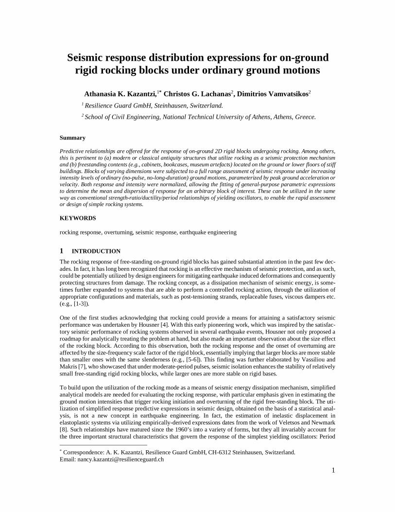
The standard rigid rocking block is assumed to be of rectangular shape, having a height equal to 2h, a base width equal to 2b (Figure 1), and mass m. It is subjected to a horizontal ground motion excitation having an acceleration time-history of 푢 (푡). Assuming that the friction coefficient of the resting plane is sufficiently high to prevent sliding, the free-standing rigid block, when it is set to rocking, it will oscillate about its pivot points O and O΄ (see Figure 1). The rocking initiation condition (i.e., the minimum horizontal ground motion acceleration to initiate uplift) may be obtained considering the static equilibrium of the block and it is equivalent to 푢 , = g ∙ tan훼 (1) where g is the acceleration of gravity and 훼 is the critical rotation, or (static) stability angle of the block:

훼 = tan (2) While the term “slenderness” is often employed for a, we will avoid using it as it carries the wrong connotations, since low-a blocks are actually slender and easier to topple, whereas high-a blocks are stocky. The value of 훼 along with the block half diagonal, R, where 푅 = √푏 + ℎ (3)

3

fully define the geometry of the rigid block. Consequently, the equation of motion that provides the angular accel-eration 휃 during the rocking motion can be expressed as (e.g., [21]), 휃 = −푝 ∙ sin(훼 ∙ sgn(휃)− 휃) +

∙ cos (훼 ∙ sgn(휃) − 휃) (4)

where, 푝 is the characteristic frequency parameter of the rigid rocking block:

푝 = ∙∙

(5)

Note that for a rigid block undergoing pure rocking, no quantity similar to the natural frequency of an oscillating pendulum can be defined [22], since the oscillation frequency strongly depends on the rocking amplitude [4]. Still, 푝 may be seen as such a measure of the block’s dynamic characteristics.

Figure 1. Geometry of the rigid rocking block. The center of mass (CM) coincides with the geometric center.

Under pure rocking (i.e. no sliding and no bouncing), when the block returns to its initial position (i.e. when rotation changes sign at 휃 = 0), impact occurs. One possible way to treat impact is by means of the coefficient of restitution, 휂, which essentially provides a relation between the pre- and post-impact angular velocities, 휃 and 휃 , respectively:

휂 = (6)

Considering the conservation of angular momentum at the instances before and after the impact, one may define an upper limit (i.e., an estimate of the minimum amount of energy dissipation) for the coefficient of restitution of a rigid rectangular rocking block as [4] 휂 = 1 − ∙ sin (훼) (7) This estimate of the coefficient of restitution should be considered as a theoretical approximation that disregards the effect of the interface material and assumes that the pertinent coefficient is a function only of the block geom-etry. More detailed and consequently more accurate models exist in the literature [23-25], yet they are all tied to the particular details of the adopted experimental set-up.

2.2 Incremental Dynamic Analysis of the rocking blocks

For evaluating the response of the rocking blocks, the standard methodology of the Incremental Dynamic Analysis (IDA, [26]) was adopted. For its implementation it requires a suite of ground motion records for performing the nonlinear response-history analyses. Thus, a total of 105 “ordinary” ground motion records were selected from the PEER-NGA [27] strong motion database. They are no-pulse, no-long-duration motions recorded on relatively firm soil. To lower scaling factors required to achieve block overturning in IDA, the records were chosen to have (a)

4

magnitude, Mw, greater than 6.2 and (b) peak ground acceleration, PGA, greater than 0.14g. With the exception of the taller blocks (i.e. those with low 푝), the overturning scaling factors for the majority were kept below 8, limiting any bias due to scaling. Consequently, this study is focused on the evaluation of the rocking response of rigid blocks that are subjected to ground motion records without distinct pulses (i.e. mostly far-field ground motions, but also near-field without forward-directivity effects) and without any long duration characteristics (i.e. excluding those generated by large magnitude events, typical of subduction zones). The records were incrementally scaled at increasing intensity levels to reveal the entire range of the structural response in question, which, for the investigated case, ranges from the initiation of rocking up to block overturning (i.e., collapse). To define an IDA curve, one needs an efficient and sufficient Intensity Measure (IM) as well as an Engineering Demand Parameter (EDP) that is representative of the structural response. For the former, two dimen-sionless IMs were adopted, as originally proposed by Dimitrakopoulos and Paraskeva [28], which will be collec-tively referred to by the symbol I:

(a) the dimensionless peak ground acceleration, 푃퐺퐴/(g ∙ tan훼), henceforth denoted as 퐼 = 푃퐺퐴/gtan훼

(b) the dimensionless peak ground velocity, 푝푃퐺푉/(g ∙ tan훼), henceforth denoted as 퐼 = 푝푃퐺푉/gtan훼

As an EDP parameter, the absolute peak rocking rotation 휃 normalized by the block stability angle 훼, i.e., 휃 =휃 /훼 [28], was adopted. The first appearance of 휃 > 0 signifies the onset of rocking. Furthermore, 휃 ≥ 1 can be taken to signify nominal overturning. The condition 휃 ≥ 1 essentially represents a statically unstable block [28] and for this reason it is considered as a threshold of particular interest for practical rocking design applications. Strictly speaking, this overturning criterion is only an approximation due to the high nonlinearity of rocking dy-namics. It has been shown [12] that it is possible for 휃 to substantially exceed 훼 without the actual occurrence of overturning; still, it is not likely. Practically, selecting any value of 휃 ≥ 0.7 would not substantially alter the statistics of overturning intensities, making the 휃 ≥ 1 criterion a viable compromise in lieu of a more complex one that could make a difference for few records without altering the overall distribution of overturning intensities. On another note, the use of normalized IM and EDP, beyond allowing the standardization of response distribution in the form of 훪 − 휃 − 푝 curves, also implies a scaling-invariance property that can help alleviate questions of scaling bias. In essence, one can view the IDA curve of any given block under a single ground motion in two ways: (a) as the EDP response of the same block under increasing IM, or (b) as the EDP response of multiple blocks having the same 푝 and decreasing 훼, under the same unscaled motion. The same property applies to R−μ−T rela-tionships, and allows us to view large values of normalized intensity R or I, either as large scaling factors corre-sponding to motions of PGA and PGV that may not be physically realizable, or as low-strength buildings and low-stability blocks. This is not a proof of scaling invariance per se, but rather a consequence of normalization that allows us to rationalize the use of larger scaling factors in IDA as equivalent to having slenderer blocks. In other words, if we want to standardize the response of both slender and stocky blocks in a compact form, we need to accept scaling invariance of response to some extent. Right beyond the attainment of overturning, nominal or otherwise, comes the issue of structural “resurrection”, whereby intensities higher than the one causing overturning can still produce non-overturning response [26]. This is only sparingly observed in hysteretic systems, yet becomes much more frequent for rocking IDA curves [33]. One may choose to terminate all IDA curves at the first occurrence of nominal overturning, or instead include results from all stable regions of response into response statistics. Given the frequent appearance of resurrections, the latter case would tend to shift the IDA quantiles slightly higher, owing to the inclusion of non-collapsing IM values higher than the first occurrence of overturning. Keeping or removing such values is a conscious decision that comes down to two issues. First of all, the effects of resurrections are only felt for 휃 ≥ 0.6. This is a value that is already close to overturning for almost all practical purposes. Therefore, considering the influence of res-urrections that occur for higher responses does not offer many advantages. Secondly the resurrections occur in a response domain that lies in the margins of validity for the simplified rocking model that was adopted herein. In particular, the assumptions for a perfectly-rigid-block on a perfectly-rigid-foundation model are not as physically consistent for structures of engineering significance undergoing such large values of response. In these response magnitudes, the model should have been able to consider some deformability of the sharp edges (toe crushing) or of the supporting surface (edge penetration) in order to claim some measure of accuracy. Given this level of epis-temic uncertainty as well as the high sensitivity of the model overturning response to such modeling details, it makes little practical sense to incorporate resurrections into our predictive equations. For such reasons, we choose to discard all results above the first attainment of overturning, offering perhaps a somewhat conservative estimate that is arguably preferable in light of model uncertainties.

5

2.3 The effect of the stability angle and restitution coefficient on the rocking response

In order to formulate a compact probabilistic model for rocking response for a variety of rigid blocks, it is important to reduce the dimensionality of the problem. According to Section 2.1, the three parameters that one needs to capture are the characteristic frequency p (or size), the stability angle α (or shape), and the restitution coefficient η. Figuring out what needs to be captured in detail and what can be removed is fundamental, and the adoption of dimensionless IMs and EDP are an important part of our approach. Without a doubt, block size matters in rocking [4-6], especially if one considers a wide range of rocking blocks and intensities levels, thus 푝 cannot be normalized out. Figures 2a-c illustrate the IDA curves in the 훪 − 휃 domain for a block having a characteristic frequency 푝 equal to one, computed for three values of a = 0.10, 0.15 and 0.25, three different ground motion records, and assuming a constant 휂 = 0.92. As can be inferred from these plots, the computed rocking response across a range of increasing intensity levels is almost identical or at worst very close for any practical application. This observation holds for both extremes, i.e., rocking initiation and overturning. The aforementioned symmetry in the response of physically similar structures has been conclusively supported for pulsive records and slender (low a) blocks [12, 28], while empirical results suggest that it adequately holds for ordinary, non-pulsive no-long-duration, records for all but the stockiest (high a) blocks [29]. By contrast, as presented in Figures 2d-f, notably different responses are computed for the aforementioned three rigid rocking blocks subjected to the same three ground motion records when altering the restitution coefficient, even by little. The coefficient of restitution may vary between 0.7 and 1.0 (e.g., [23, 30-33]), yet, as discussed in Section 2.1, pinning down an exact value is difficult outside of controlled experiments. Treating it as a source of uncertainty in the first-order sense [34], i.e., assuming that the unknown value does not change the central value of response but may only inflate its dispersion, leads to the obvious question of what that increase might be. Past observations [5, 13, 14] have reported an overall moderate effect of the restitution coefficient, as opposed to other system parameters. Given the square-root-sum-of-squares aggregation of dispersions and the sizeable dispersions already observed due to record-to-record variability, it can be argued that the effect of an uncertain restitution coefficient can be disregarded. Therefore, for the remainder of our work, a typical value of 휂 = 0.92 was assumed [3, 13], implying that every impact results in a total energy loss of 8%. This choice is anticipated to have only a moderate effect on the proposed rocking response probabilistic model, at least for restitution values that do not significantly deviate from the assumed constant value [5].

(a) (b) (c)

(d) (e) (f)

Figure 2. IDAs for three different earthquake records: (a-c) with constant coefficient of restitution and (d-f) with the a-dependent coefficient of restitution evaluated from Eq. (7) as proposed by Housner [4] for a rigid block with 푝=1s-1.

6

2.4 Rocking response evaluation

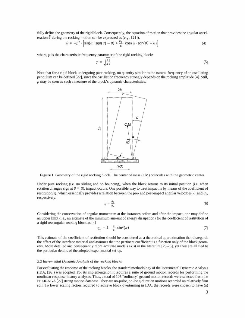
For undertaking a detailed probabilistic assessment on the response of on-ground rocking blocks, a total of 44 rectangular rigid blocks were considered (see Figure 3). They have frequency parameters 푝 that range from 0.7s-1 to 5.0s-1. This range essentially corresponds to rocking blocks having half-diagonal R values spanning between 15.015m and 0.294m. To put it differently, considering a block stability angle of 훼 = 0.22rad, which translates to a numerically equivalent aspect ratio b / h, the resulting blocks have a total base width (2b) and total height (2h) within the following ranges:

p=0.7s-1 corresponds to a block with 2b ≈ 6.55m, 2h ≈ 29.31m

p=5.0s-1 corresponds to a block with 2b ≈ 0.13m, 2h ≈ 0.57m

The considered characteristic frequency range was thus selected to reflect a wide spectrum of systems that are likely to exhibit rocking. Hence, the lower bound of 푝 (0.7s-1) could well represent a rocking bridge pier, whereas the upper bound (5.0s-1) could be a freestanding museum artefact. As mentioned earlier, in all analyses the coeffi-cient of restitution was assumed to be constant at 휂 = 0.92. Regarding 훼, given that in the dimensionless EDP-IM domain its effect on the median response is trivial for all applications of practical interest, a single constant value was assumed for all analyses. In other words, the considered blocks differ in size (p), that matters a lot, but not in shape (훼), that only has a minor effect on the evaluated responses. Τhe 44 rocking blocks were subjected to the same set of 105 horizontal components, each one randomly selected from each of the 105 considered ground motion record pairs. It should be noted that the rocking response was studied by utilizing a 2D model of the rocking block. Each record was incrementally scaled at increasing intensity levels of PGA every 0.01g, starting from the value of gtan훼 where rocking is initiated. At every intensity level, the rocking response was computed by solving Equation (4) using the software developed by Vassiliou [35] to estimate the peak rocking angle 휃 . Incrementation of intensities was terminated for each record when 휃 became greater than 훼.

(a) (b)

Figure 3. (a) A schematic representation of the 44 rocking blocks that were considered in this study and (b) the dimensions of three blocks with different 푝 values. Large blocks are associated with small 푝 values and vice versa.

The response estimates of the rocking motion are evaluated against two versions of each of the two IMs employed. First, are arbitrary-component IMs, i.e., PGA and PGV estimated for the single horizontal component of each ground motion record pair employed in the analyses. Henceforth, these will be termed PGAarb and PGVarb. Sec-ondly, geometric mean (or geomean) component IMs were also employed. These are estimated via the square root of the product of the two PGA or PGV values estimated from both horizontal components of each record, and they

7

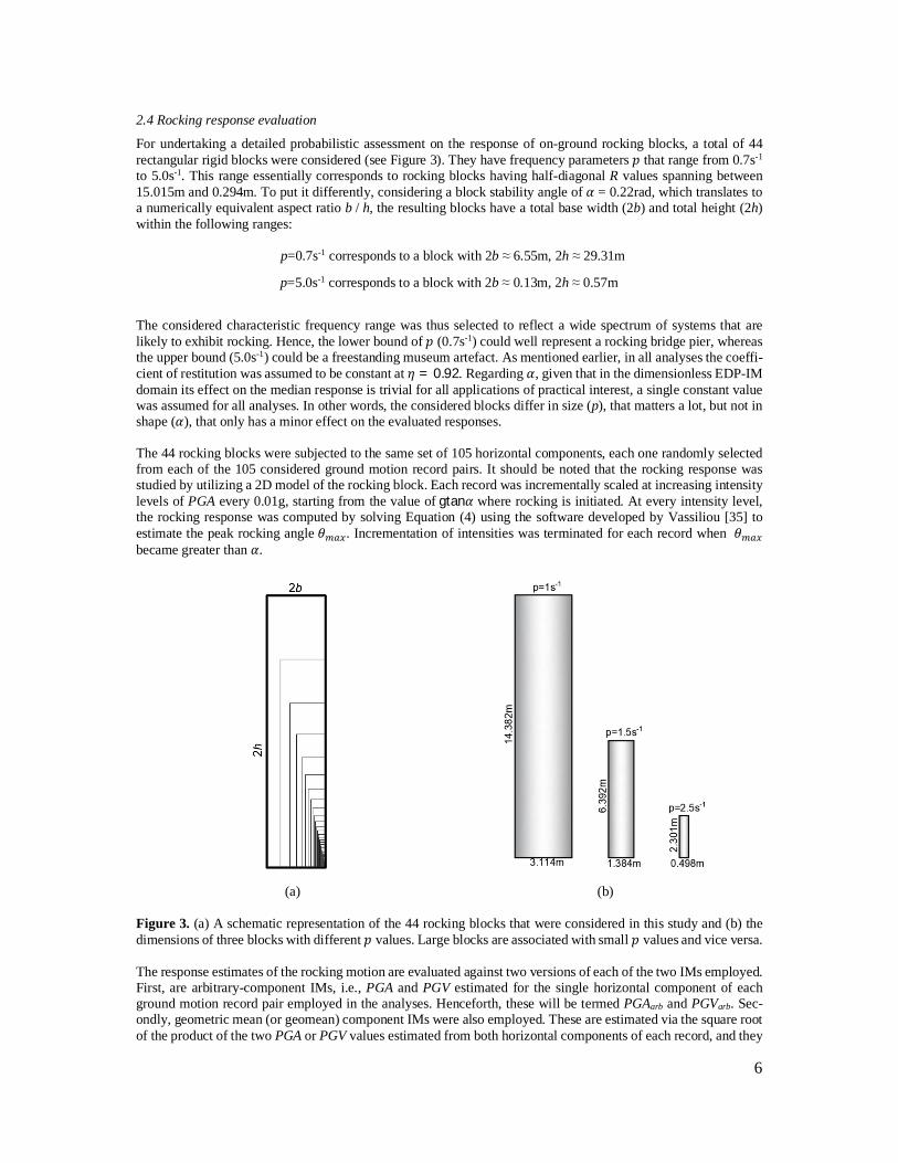
will be termed PGAgm and PGVgm. Arbitrary-component estimates are better suited to estimating the response in a pure 2D problem, where one applies a suite of records in the horizontal direction and directly employs the PGA or PGV of the applied motions to estimate the response. Geomean-component expressions conform to the modern paradigm of probabilistic seismic hazard assessment, whereby hazard maps, hazard curves, uniform hazard spectra and ground motion fields are typically offered in rotation-invariant values [36], which for all practical purposes are numerically equivalent to geomean estimates [37]. Despite their relatively small difference, knowing when to employ each type of IM is important to avoid bias in probabilistic response assessment [38]. Figure 4a illustrates a set of 105 IDA curves that were computed for a rigid rocking block with 푝 = 1.2s-1. The results are shown for the dimensionless arbitrary-component intensity of 훪 , = 푃퐺퐴 /gtan훼 and 휃. As can be inferred by inspecting this plot, the record-to-record variability is dominant. The only deterministic point is the rocking initiation that occurs for all records exactly at 푃퐺퐴 = gtan훼 or at 훪 , = 1. Note that shifting to the geomean intensity, 훪 , , removes even that last shred of determinism, as 훪 , = 1 only approximately corre-sponds to the onset of rocking, since the averaging of the IMs from two horizontal components (where only one is employed and the other is discarded) introduces some randomness. Higher levels of response, and especially over-turning, are characterized by considerably higher dispersion values. Individual records can overturn the block at intensities 훪 , that can range from 1.5 to 17 or higher. These observations further support that the probabilistic treatment of the problem is the only meaningful route for effectively treating the rocking problem. Figure 4b illustrates for the aforementioned block, the median IDA curve (i.e., the central tendency) along with the 16% and 84% fractile IDA curves (evaluated through horizontal stripes, i.e., on an EDP|IM basis, see [29, 39]), which provide an estimate of the dispersion. As can be inferred by inspecting the plots presented in Figure 4, contrary to the record-specific IDAs that are highly variable and non-monotonic, their percentiles are much smoother, offering a more manageable domain for describing the demand via simple equations.

(a) (b)

Figure 4. (a) 105 IDA curves and (b) 16%, 50%, 84% actual (solid) and smoothed (dashed) IDA percentiles for

a rigid rocking block with 푝 = 1.2 s-1. In fact, as illustrated in Figure 5a, the high dependence of the rocking response on distinct ground motion record characteristics could lead to rocking IDA curves having a highly weaving behavior [26]. Figure 5b captures the median IDA curves (evaluated in an EDP|IM basis) for three sets of 10, 40 and 70 ground motion records that were randomly selected from the full 105 record set. Apparently, the large-scale features of the individual IDAs are increasingly smoothened down as we turn to the medians of larger sets of records; all that remains is a low-ampli-tude high-frequency “noise” around each median. For all three fractile curves (16/50/84), IM is a near-monotonic function of the EDP, while the “noise” tends to disappear when increasing the number of the records [33]. Thus, in order to accelerate the smoothing process, instead of running IDAs for an inefficient large number of ground motion records (for instance 3000 individual records), a monotone spline smoother [40-41] was applied to the fractile IDA curves (Figure 4b) to effectively dampen out the residual “noise”.

8

(a) (b)

Figure 5. (a) IDA curves for three individual ground motion records and (b) median IDA curves for three sets of 10, 40 and 70 randomly selected ground motion records.

3 REGRESSION ANALYSIS ON ROCKING DEMANDS

For practical applications (either design or assessment) utilizing rocking as a means of seismic protection, it is desirable to have a simple set of equations that could be used to provide robust estimates for the distribution of the rocking block seismic demand. To accomplish this goal, nonlinear regression analysis was employed to develop 훪 − 휃 − 푝 expressions for the median and dispersion (standard deviation of the log of the data) evaluated on an EDP|IM basis. These two statistics are meant to directly provide a lognormal distribution, which has been found to provide a statistically significant representation for most rocking applications [20, 29], but they can also be employed to fit any two-parameter distribution of interest (Gumbel, Weibull, Pareto, etc.). The proposed equations are deemed to be valid for rigid non-stocky blocks having a 푝 that ranges from 0.7s-1 up to 5.0s-1. The results are presented here for four IMs, these being the dimensionless PGAs and PGVs defined either in an arbitrary or in a geometric mean sense.

3.1 Median response fitting for 푃퐺퐴

A three-fold functional form [see Equations (8a-b)] is used to relate the median dimensionless EDP, 휃 , with the dimensionless PGA intensity, 퐼 , which is either 푃퐺퐴 /gtan훼 or 푃퐺퐴 /gtan훼. The first part captures the dis-tinctive transition from the very initiation of motion to actual rocking, herein idealized as a linear segment; the second part is meant to represent the main body of rocking response up to overturning, naturally becoming the more complex of the three; the third captures the first occurrence of nominal overturning (i.e., defined as the first attainment of a statically unstable state). The median intensity level where overturning occurs is fitted via a sepa-rate regression, using an expression that is only a function of 푝. This intensity level also sets the upper bound, 퐼 , , for the domain of the second part of the three-fold equation.

휃 (퐼 ) =휃 (퐼 − 퐶 )/(1.2 −퐶 ) for 퐶 ≤ 퐼 ≤ 1.20.1 ∙ 퐴 ∙ (퐼 − 퐶 ) . − for 1.2 < 퐼 < 퐼 ,

1 for 퐼 ≥ 퐼 ,

(8a)

Note that despite using least-squares estimation, we do not employ regression per se to derive the entire distribution in one step. Instead, we are using curve-fitting to derive customized expressions per each statistic of interest, allowing us to casually invert Equation (8a), to determine the median intensity, 퐼 , given 휃:

퐼 (휃) =

⎩⎪⎨

⎪⎧퐶 + (1.2− 퐶 )휃/휃 for 0 ≤ 휃 ≤ 휃

. ∙

.+ 퐶 for 휃 < 휃 < 1

퐼 , for 휃 ≥ 1

(8b)

9

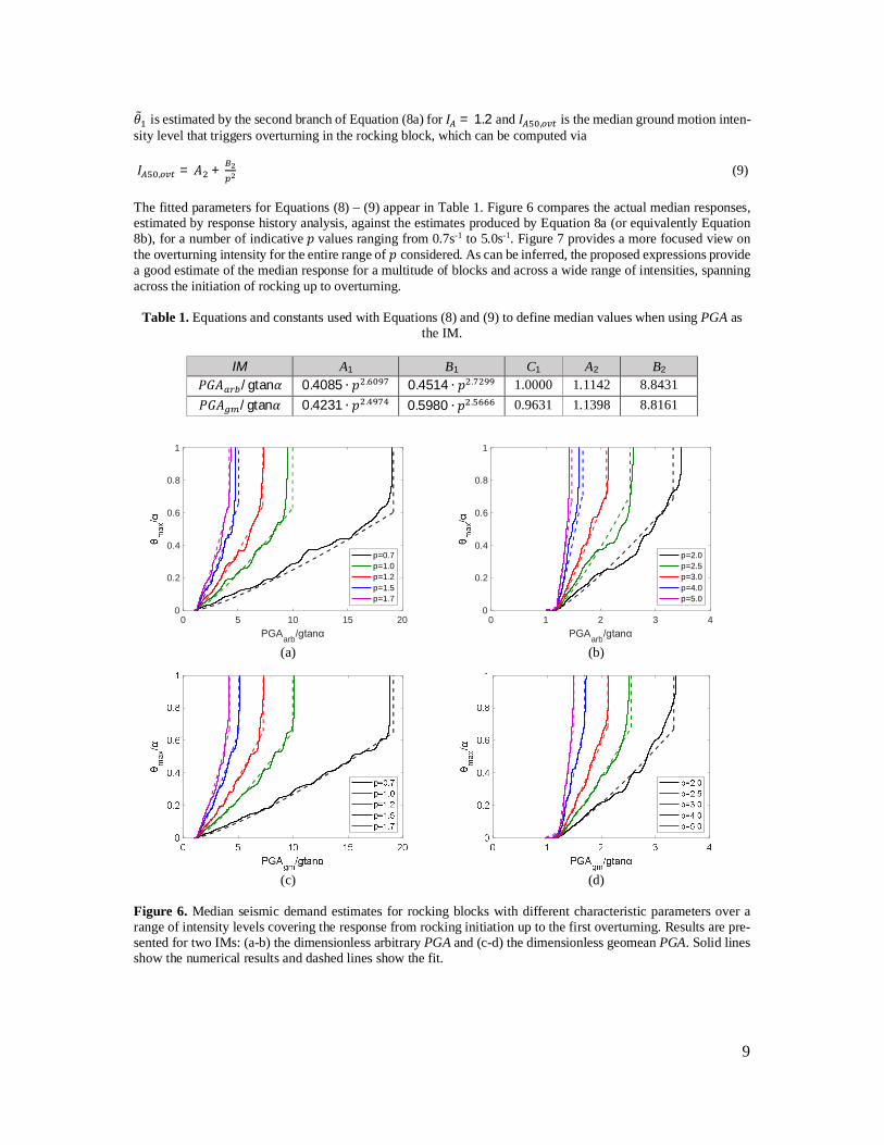
휃 is estimated by the second branch of Equation (8a) for 퐼 = 1.2 and 퐼 , is the median ground motion inten-sity level that triggers overturning in the rocking block, which can be computed via 퐼 , = 퐴 + (9) The fitted parameters for Equations (8) – (9) appear in Table 1. Figure 6 compares the actual median responses, estimated by response history analysis, against the estimates produced by Equation 8a (or equivalently Equation 8b), for a number of indicative 푝 values ranging from 0.7s-1 to 5.0s-1. Figure 7 provides a more focused view on the overturning intensity for the entire range of 푝 considered. As can be inferred, the proposed expressions provide a good estimate of the median response for a multitude of blocks and across a wide range of intensities, spanning across the initiation of rocking up to overturning.

Table 1. Equations and constants used with Equations (8) and (9) to define median values when using PGA as the IM.

IM A1 B1 C1 A2 B2

푃퐺퐴 /gtan훼 0.4085 ∙ 푝 . 0.4514 ∙ 푝 . 1.0000 1.1142 8.8431 푃퐺퐴 /gtan훼 0.4231 ∙ 푝 . 0.5980 ∙ 푝 . 0.9631 1.1398 8.8161

(a) (b)

(c) (d)

Figure 6. Median seismic demand estimates for rocking blocks with different characteristic parameters over a range of intensity levels covering the response from rocking initiation up to the first overturning. Results are pre-sented for two IMs: (a-b) the dimensionless arbitrary PGA and (c-d) the dimensionless geomean PGA. Solid lines show the numerical results and dashed lines show the fit.

0 5 10 15 20PGAarb/gtanα

0

0.2

0.4

0.6

0.8

1

p=0.7p=1.0p=1.2p=1.5p=1.7

0 1 2 3 4PGAarb/gtanα

0

0.2

0.4

0.6

0.8

1

p=2.0p=2.5p=3.0p=4.0p=5.0

10

(a) (b)

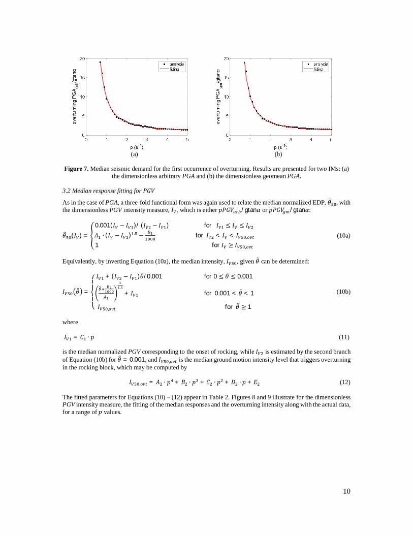
Figure 7. Median seismic demand for the first occurrence of overturning. Results are presented for two IMs: (a)

the dimensionless arbitrary PGA and (b) the dimensionless geomean PGA. 3.2 Median response fitting for 푃퐺푉

As in the case of PGA, a three-fold functional form was again used to relate the median normalized EDP, 휃 , with the dimensionless PGV intensity measure, 퐼 , which is either 푝푃퐺푉 /gtan훼 or 푝푃퐺푉 /gtan훼:

휃 (퐼 ) =0.001(퐼 − 퐼 )/ (퐼 − 퐼 ) for 퐼 ≤ 퐼 ≤ 퐼퐴 ∙ (퐼 − 퐼 ) . − for 퐼 < 퐼 < 퐼 ,

1 for 퐼 ≥ 퐼 ,

(10a)

Equivalently, by inverting Equation (10a), the median intensity, 퐼 , given 휃 can be determined:

퐼 휃 =

⎩⎪⎨

⎪⎧ 퐼 + (퐼 − 퐼 )휃/0.001 for 0 ≤ 휃 ≤ 0.001

.

+ 퐼 for 0.001 < 휃 < 1

퐼 , for 휃 ≥ 1

(10b)

where 퐼 = 퐶 ∙ 푝 (11) is the median normalized PGV corresponding to the onset of rocking, while 퐼 is estimated by the second branch of Equation (10b) for 휃 = 0.001, and 퐼 , is the median ground motion intensity level that triggers overturning in the rocking block, which may be computed by 퐼 , = 퐴 ∙ 푝 + 퐵 ∙ 푝 + 퐶 ∙ 푝 + 퐷 ∙ 푝 + 퐸 (12) The fitted parameters for Equations (10) – (12) appear in Table 2. Figures 8 and 9 illustrate for the dimensionless PGV intensity measure, the fitting of the median responses and the overturning intensity along with the actual data, for a range of 푝 values.

11

(a) (b)

(c) (d)

Figure 8. Median seismic demand estimates for rocking blocks with different characteristic parameters over a range of intensity levels covering the response from rocking initiation up to the first overturning. Results are pre-sented for two IMs: (a-b) the dimensionless arbitrary PGV and (c-d) the dimensionless geomean PGV. Solid lines show the numerical results and dashed lines show the fit.

(a) (b)

Figure 9. Median intensity at the first occurrence of overturning. Results are presented for two IMs: (a) the di-

mensionless arbitrary PGV and (b) the dimensionless geomean PGV.

0 1 2 3 4 5

p (s-1)

0.4

0.6

0.8

1

1.2analysisfitting

12

Table 2. Equations and constants used with Equations (10) – (12) to define to define median values when using PGV as the IM.

IM A1 B1

푝푃퐺푉 /gtan훼 0.0468 ∙ 푝 − 0.3018 ∙ 푝 + 1.7193 ∙ 푝 − 0.3845

−0.1743 ∙ 푝 + 3.2451 ∙ 푝 +1.4941 ∙ 푝 − 2.4536

푝푃퐺푉 /gtan훼 0.0661 ∙ 푝 + 0.9607 ∙ 푝 +0.0531

3.0970 ∙ 푝 + 2.3314 ∙ 푝 −2.7855

IM C1 A2 B2 C2 D2 E2 푝푃퐺푉 /gtan훼 0.0919 0.0147 -0.1899 0.8917 -1.7937 1.9373 푝푃퐺푉 /gtan훼 0.0905 0.0096 -0.1282 0.6319 -1.3498 1.6764

3.3 Dispersion fitting for 푃퐺퐴

To offer a comprehensive probabilistic model of the rocking response via a two-parameter distribution model, a measure of dispersion is required. Targeting a typical lognormal approximation of seismic response, the standard deviation of the logarithm of the data was chosen, which can be conveniently approximated as the half-distance between the logarithm of the 16% and 84% percentiles. There is little incentive to offer the dispersion of EDP for values of the given IM: The “infinite” 휃 responses appearing at low intensities simply invalidate any meaningful quantification. On the other hand, targeting the dispersion of IM|EDP is always tractable, as well as practical, since this quantity directly translates to the fragility dispersion for exceeding the given value of EDP. Apparently, for the dimensionless 푃퐺퐴 very similar trends are detected both for the arbitrary (Figures 10a-b) and the geomean quantities (Figures 10c-d). At the initiation of rocking, the dispersion is zero for the arbitrary 푃퐺퐴 , since for all blocks the rocking initiation occurs exactly at a normalized intensity level 훪 , = 1 (see Figures 6a-b). By contrast, for 푃퐺퐴 , the dispersion associated with the variability around the median intensity level that triggers the rocking motion is approximately equal to 0.2 for all the considered blocks. At higher intensity levels, where the rocking blocks are on the verge of collapse (i.e., overturning) the dispersion takes values in the order of 0.8 for the largest blocks considered in this study (i.e., p = 0.7s-1) and drops to around 0.2 for the smallest blocks (i.e., p = 5.0s-1). Similarly to the approach adopted for fitting the median, a two-part expression is formed by undertaking a nonlin-ear regression analysis for the dispersion of 퐼 , and 퐼 , as a function of p, taking η = 0.92:

훽 (휃) =퐴 · + 퐶 for 0 ≤ 휃 ≤ 0.8

훽 휃 = 0.8 elsewhere (13)

where the relevant parameters appear in Table 3. Note that this dispersion estimate for the normalized PGA quan-tities is numerically equivalent to the one of the respective unnormalized PGA quantities by virtue of g and tana being constants.

Table 3. Equations and constants used with Equation (13) to define the PGA dispersion given the EDP.

IM A1 B1 C1

푃퐺퐴 /gtan훼 0.0420 ∙ 푝 − 0.3719 ∙ 푝 + 0.6205 ∙ 푝 + 1.6220

0.0088 ∙ 푝 − 0.1302 ∙ 푝 + 0.5635 ∙ 푝 + 0.0581 0

푃퐺퐴 /gtan훼 0.0529 ∙ 푝 − 0.4774 ∙ 푝 + 0.9416 ∙ 푝 + 0.9226

0.0292 ∙ 푝 − 0.2602 ∙ 푝 + 0.9622 ∙ 푝 − 0.2140 0.1763

13

(a) (b)

(c) (d)

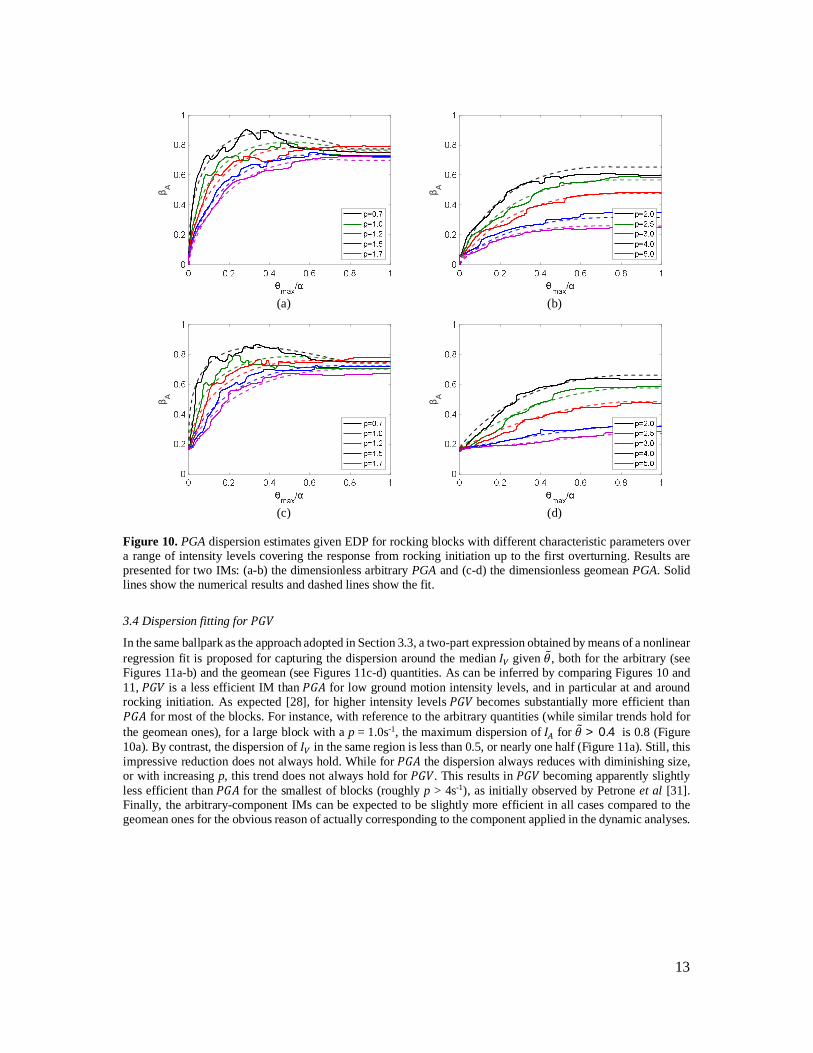
Figure 10. PGA dispersion estimates given EDP for rocking blocks with different characteristic parameters over a range of intensity levels covering the response from rocking initiation up to the first overturning. Results are presented for two IMs: (a-b) the dimensionless arbitrary PGA and (c-d) the dimensionless geomean PGA. Solid lines show the numerical results and dashed lines show the fit.

3.4 Dispersion fitting for 푃퐺푉

In the same ballpark as the approach adopted in Section 3.3, a two-part expression obtained by means of a nonlinear regression fit is proposed for capturing the dispersion around the median 퐼 given 휃, both for the arbitrary (see Figures 11a-b) and the geomean (see Figures 11c-d) quantities. As can be inferred by comparing Figures 10 and 11, 푃퐺푉 is a less efficient IM than 푃퐺퐴 for low ground motion intensity levels, and in particular at and around rocking initiation. As expected [28], for higher intensity levels 푃퐺푉 becomes substantially more efficient than 푃퐺퐴 for most of the blocks. For instance, with reference to the arbitrary quantities (while similar trends hold for the geomean ones), for a large block with a p = 1.0s-1, the maximum dispersion of 퐼 for 휃 > 0.4 is 0.8 (Figure 10a). By contrast, the dispersion of 퐼 in the same region is less than 0.5, or nearly one half (Figure 11a). Still, this impressive reduction does not always hold. While for 푃퐺퐴 the dispersion always reduces with diminishing size, or with increasing p, this trend does not always hold for 푃퐺푉. This results in 푃퐺푉 becoming apparently slightly less efficient than 푃퐺퐴 for the smallest of blocks (roughly p > 4s-1), as initially observed by Petrone et al [31]. Finally, the arbitrary-component IMs can be expected to be slightly more efficient in all cases compared to the geomean ones for the obvious reason of actually corresponding to the component applied in the dynamic analyses.

β A β A

β A β A

14

(a) (b)

(c) (d)

Figure 11. PGV dispersion estimates given EDP for rocking blocks with different characteristic parameters over a range of intensity levels covering the response from rocking initiation up to the first overturning. Results are presented for two IMs: (a-b) the dimensionless arbitrary PGV and (c-d) the dimensionless geomean PGV. Solid lines show the numerical results and dashed lines show the fit. It should be also noted here that due to the nonmonotonic trends observed in the dispersion evaluated for 푃퐺푉, the fitting cannot be as good as in the case of the well-behaved 푃퐺퐴. Nevertheless, the fit is considered satisfactory and slightly on the conservative side where large deviations are concerned. Hence, we refrained from proposing a more complex equation to better capture the observed trends:

훽 (휃) =퐷 − 퐴 ·

( ) for 0 ≤ 휃 ≤ 0.7

훽 휃 = 0.7 elsewhere (14)

with the relevant parameters appearing in Table 4. Similarly to the PGA case, this dispersion also holds for the respective unnormalized 푃퐺푉 quantities.

Table 4. Equations and constants used with Equation (14) to define the PGV dispersion given the EDP.

IM A1 B1 C1 D1 푝푃퐺푉 /gtan훼 0.0090 ∙ 푝 . 0.1750 ∙ 푝 . 4 0.4880 푝푃퐺푉 /gtan훼 0.0108 ∙ 푝 . 0.1018 ∙ 푝 . 3 0.4613

4 VALIDATION

The proposed equations in Section 3 were tested against three generic blocks that were not employed for fitting. They were chosen to roughly resemble columns from temples of classical antiquity. The first column (Column No

β V β V

β V β V

15

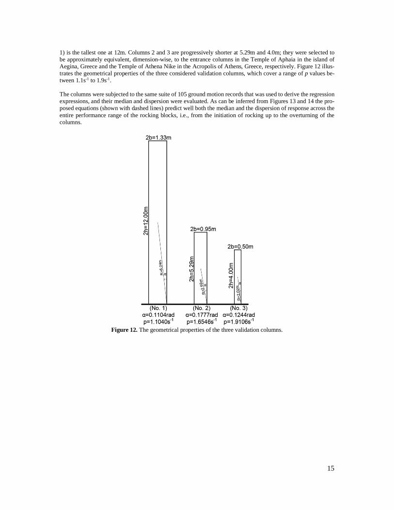
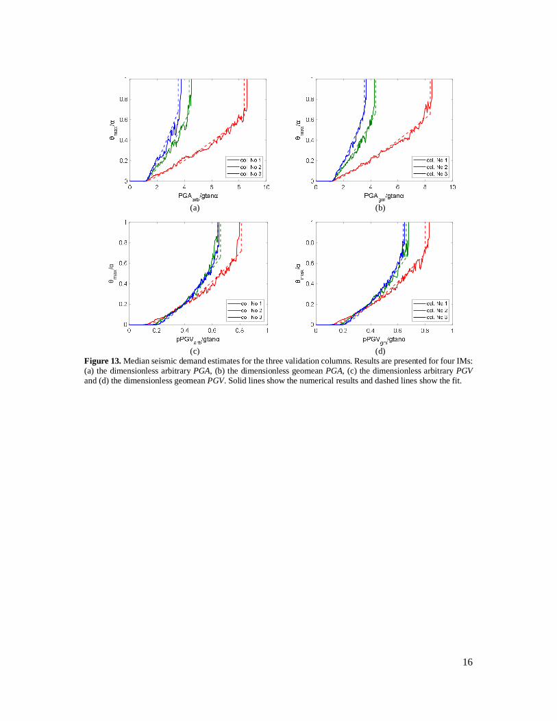
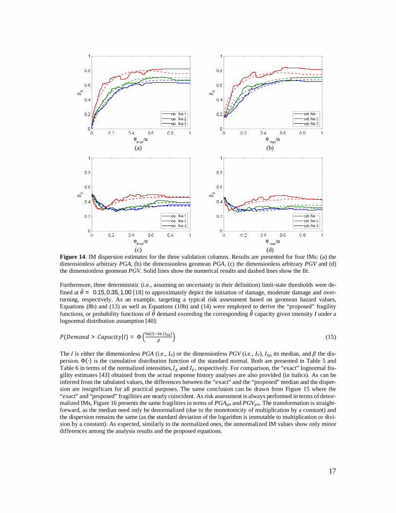
1) is the tallest one at 12m. Columns 2 and 3 are progressively shorter at 5.29m and 4.0m; they were selected to be approximately equivalent, dimension-wise, to the entrance columns in the Temple of Aphaia in the island of Aegina, Greece and the Temple of Athena Nike in the Acropolis of Athens, Greece, respectively. Figure 12 illus-trates the geometrical properties of the three considered validation columns, which cover a range of p values be-tween 1.1s-1 to 1.9s-1. The columns were subjected to the same suite of 105 ground motion records that was used to derive the regression expressions, and their median and dispersion were evaluated. As can be inferred from Figures 13 and 14 the pro-posed equations (shown with dashed lines) predict well both the median and the dispersion of response across the entire performance range of the rocking blocks, i.e., from the initiation of rocking up to the overturning of the columns.

Figure 12. The geometrical properties of the three validation columns.

16

(a) (b)

(c) (d)

Figure 13. Median seismic demand estimates for the three validation columns. Results are presented for four IMs: (a) the dimensionless arbitrary PGA, (b) the dimensionless geomean PGA, (c) the dimensionless arbitrary PGV and (d) the dimensionless geomean PGV. Solid lines show the numerical results and dashed lines show the fit.

θ max

/α

17

(a) (b)

(c) (d)

Figure 14. IM dispersion estimates for the three validation columns. Results are presented for four IMs: (a) the dimensionless arbitrary PGA, (b) the dimensionless geomean PGA, (c) the dimensionless arbitrary PGV and (d) the dimensionless geomean PGV. Solid lines show the numerical results and dashed lines show the fit.

Furthermore, three deterministic (i.e., assuming no uncertainty in their definition) limit-state thresholds were de-fined at 휃 = 0.15, 0.35, 1.00 [18] to approximately depict the initiation of damage, moderate damage and over-turning, respectively. As an example, targeting a typical risk assessment based on geomean hazard values, Equations (8b) and (13) as well as Equations (10b) and (14) were employed to derive the “proposed” fragility functions, or probability functions of 휃 demand exceeding the corresponding 휃 capacity given intensity I under a lognormal distribution assumption [40]: 푃(퐷푒푚푎푛푑 > 퐶푎푝푎푐푖푡푦|퐼) = Φ ( ) ( ) (15) The 퐼 is either the dimensionless PGA (i.e., IA) or the dimensionless PGV (i.e., IV), 퐼 its median, and 훽 the dis-persion. Φ(∙) is the cumulative distribution function of the standard normal. Both are presented in Table 5 and Table 6 in terms of the normalized intensities, 퐼 and 퐼 , respectively. For comparison, the “exact” lognormal fra-gility estimates [43] obtained from the actual response history analyses are also provided (in italics). As can be inferred from the tabulated values, the differences between the “exact” and the “proposed” median and the disper-sion are insignificant for all practical purposes. The same conclusion can be drawn from Figure 15 where the “exact” and “proposed” fragilities are nearly coincident. As risk assessment is always performed in terms of denor-malized IMs, Figure 16 presents the same fragilities in terms of PGAgm and PGVgm. The transformation is straight-forward, as the median need only be denormalized (due to the monotonicity of multiplication by a constant) and the dispersion remains the same (as the standard deviation of the logarithm is immutable to multiplication or divi-sion by a constant). As expected, similarly to the normalized ones, the unnormalized IM values show only minor differences among the analysis results and the proposed equations.

β A β A

β V β V

18

Table 5. PGAgm-based fragility estimates for the three limit-states defined at normalized angles of 0.15, 0.35, and 1.0. Values in italics show the parameters obtained via directly processing the response history analyses data and consequently assuming a lognormal fit.

Column 휃 = 0.15 휃 = 0.35 휃 = 1.00 퐼 * 훽 ** 퐼 훽 퐼 훽

No.1 3.31 (3.44) 0.60 (0.63) 5.49 (5.65) 0.74 (0.75) 8.37 (8.47) 0.75 (0.70) No.2 2.08 (2.19) 0.44 (0.54) 3.04 (3.33) 0.61 (0.61) 4.36 (4.46) 0.71 (0.65) No.3 1.84 (1.92) 0.40 (0.49) 2.56 (2.83) 0.55 (0.58) 3.55 (3.81) 0.67 (0.64)

* Equation (8b) ** Equation (13) Table 6. PGVgm-based fragility estimates for the three limit-states defined at normalized angles of 0.15, 0.35, and 1.0. Values in italics show the parameters obtained via directly processing the response history data and fitting a lognormal distribution.

Column 휃 = 0.15 휃 = 0.35 휃 = 1.00 퐼 * 훽 ** 퐼 훽 퐼 훽

No.1 0.35 (0.35) 0.33 (0.34) 0.54 (0.57) 0.40 (0.44) 0.80 (0.84) 0.44 (0.46) No.2 0.35 (0.34) 0.29 (0.29) 0.49 (0.51) 0.30 (0.32) 0.66 (0.67) 0.35 (0.37) No.3 0.35 (0.34) 0.30 (0.31) 0.48 (0.50) 0.27 (0.30) 0.64 (0.66) 0.31 (0.34)

* Equation (10b) ** Equation (14)

(a) col. No. 1 (b) col. No. 3

(c) col. No. 1 (d) col. No. 3

Figure 15. Fragility curves for columns No. 1 and No. 3 versus using the dimensionless (a-b) PGAgm and (c-d) PGVgm. Solid lines present the estimates obtained via Eq. (8b), (10b), (13), (14), while the dashed ones the lognor-mal fit of the analysis results.

19

(a) col. No. 1 (b) col. No. 3

(c) col. No. 1 (d) col. No. 3

Figure 16. Fragility curves for columns 1 and 3 versus using the unnormalized (a-b) PGAgm and (c-d) PGVgm. Solid lines present the estimates via Eq. (8b), (10b), (13), (14), while the dashed ones the lognormal fit of the analysis results.

5 CONCLUSIONS

Α comprehensive set of equations is offered for estimating the seismic response statistics of free-standing rigid rocking blocks subjected to ordinary ground motions. The equations were obtained by means of nonlinear regres-sion analyses on the computed seismic responses for a range of block parameters. It is showcased that, if the rocking response is normalized by the stability angle of the block (i.e., 휃) and the intensity of the ground motion is expressed in a dimensionless form (i.e., 훪), then, assuming a constant restitution coefficient of the order of 0.92, the distribution of response can be compactly evaluated as a function of only the ground motion intensity and the characteristic frequency, or block size (i.e., 푝). The resulting 훪 − 휃 − 푝 expressions for estimating the rocking re-sponse are analogous to the R−μ−T relationships that are used for estimating the maximum inelastic displacement of yielding oscillators, and can be directly employed for performance-based design and assessment.

6 ACKNOWLEDGEMENTS

The authors would like to thank Drs E.G. Dimitrakopoulos and M.F. Vassiliou for providing comments and con-structive suggestions for improving this research work. Dr. Vassiliou is also acknowledged for providing the soft-ware for undertaking the numerical study on the rocking oscillators under earthquake excitations.

7 FUNDING

This research has been cofinanced by the European Regional Development Fund of the European Union and Greek National Funds through the Operational Program Competitiveness, Entrepreneurship and Innovation, under the call RESEARCH – CREATE – INNOVATE (project code: Τ1EDK-00956), project: “ARCHYTAS”. Financial support has been also provided by the European Framework Programme for Research and Innovation (Horizon 2020) under the “HYPERION” project with Grant Agreement number 821054.

20

8 DATA AVAILABILITY STATEMENT

The data that support the findings of this study are available from the corresponding author upon reasonable re-quest.

9 REFERENCES

[1] Eatherton MR, Hajjar JF, Deierlein GG, Krawinkler H, Billington S, Ma X. Controlled rocking of steel-framed buildings with replaceable energy-dissipating fuses, Proc., 14th World Conference on Earthquake Engineering, Beijing, China, 2008.

[2] Dimitrakopoulos EG, DeJong MJ. Seismic overturning of rocking structures with external viscous dampers. In: Papadrakakis M., Fragiadakis M., Plevris V. (eds) Computational Methods in Earthquake Engineering. Com-putational Methods in Applied Sciences, vol 30. Springer, Dordrecht. https://doi.org/10.1007/978-94-007-6573-3_12, 2013.

[3] Giouvanidis AI, Dimitrakopoulos EG. Seismic performance of rocking frames with flag-shaped hysteretic be-havior. Journal of Engineering Mechanics (ASCE), 143(5): 04017008, 2017. https://doi.org/10.1061/(ASCE)EM.1943-7889.0001206.

[4] Housner GW. The behavior of inverted pendulum structures during earthquakes. Bulletin of the Seismological Society of America, 53(2): 403–417, 1963.

[5] Yim C-S, Chopra AK, Penzien J. Rocking response of rigid blocks to earthquakes. Earthquake Engineering and Structural Dynamics, 8(6):565–587, 1980. https://doi.org/10.1002/eqe.4290080606.

[6] Ishiyama Y. Motions of rigid bodies and criteria for overturning by earthquake excitations. Earthquake Engi-neering and Structural Dynamics, 10(5): 635–650, 1982. https://doi.org/10.1002/eqe.4290100502.

[7] Vassiliou MF, Makris N. Analysis of the rocking response of rigid blocks standing free on a seismically isolated base. Earthquake Engineering and Structural Dynamics, 41(2): 177–196, 2012. https://doi.org/10.1002/eqe.1124.

[8] Veletsos AS, Newmark NM. Effect of inelastic behavior on the response of simple systems to earthquake mo-tions, Proc., 2nd World Conference on Earthquake Engineering, Japan, Vol. 2, 895–912, 1960.

[9] Vamvatsikos D, Cornell CA. Direct estimation of the seismic demand and capacity of oscillators with multi-linear static pushovers through IDA. Earthquake Engineering and Structural Dynamics, 35(9): 1097–1117, 2006. https://doi.org/10.1002/eqe.573.

[10] Ruiz-Garcia J, Miranda E. Probabilistic estimation of maximum inelastic displacement demands for perfor-mance-based design. Earthquake Engineering and Structural Dynamics, 36(9): 1235–1254, 2007. https://doi.org/10.1002/eqe.680.

[11] Makris N, Black CJ. Dimensional analysis of rigid-plastic and elastoplastic structures under pulse-type exci-tations. Journal of Engineering Mechanics (ASCE), 130(9):1006–1018, 2004. https://doi.org/10.1061/(ASCE)0733-9399(2004)130:9(1006).

[12] Dimitrakopoulos EG, DeJong MJ. Revisiting the rocking block: closed-form solutions and similarity laws. Proceedings of the Royal Society A: Mathematical, Physical and Engineering Sciences, 468(2144):2294–2318, 2012. https://doi.org/10.1098/rspa.2012.0026.

[13] Giouvanidis AI, Dimitrakopoulos EG. Rocking amplification and strong-motion duration. Earthquake Engi-neering and Structural Dynamics, 47(10):2094–2116, 2018. https://doi.org/10.1002/eqe.3058.

[14] Bachmann JA, Strand M, Vassiliou MF, Broccardo M, Stojadinovic´ B. Is rocking motion predictable? Earth-quake Engineering and Structural Dynamics, 47(2):535–552, 2017. https://doi.org/10.1002/eqe.2978.

[15] Loli M, Knappett JA, Brown MJ, Anastasopoulos I, Gazetas G. Centrifuge modeling of rocking-isolated inelastic RC bridge piers. Earthquake Engineering and Structural Dynamics, 43(15):2341–2359, 2014. https://doi.org/10.1002/eqe.2451.

[16] Psycharis IN, Papastamatiou DY, Alexandris AP. Parametric investigation of the stability of classical columns under harmonic and earthquake excitations. Earthquake Engineering and Structural Dynamics, 29(8):1093–1109, 2000. https://doi.org/10.1002/1096-9845(200008)29:8⟨1093::AID-EQE953⟩3.0.CO;2-S.

21

[17] Stefanou I, Psycharis IN, Georgopoulos I-O. Dynamic response of reinforced masonry columns in classical monuments. Construction and Building Materials, 25(12):4325–4337, 2011. https://doi.org/10.1016/j.conbuildmat.2010.12.042.

[18] Psycharis IN, Fragiadakis M, Stefanou I. Seismic reliability assessment of classical columns subjected to near-fault ground motions. Earthquake Engineering and Structural Dynamics, 42(14):2061–2079, 2013. https://doi.org/10.1002/eqe.2312.

[19] Papadopoulos K, Vintzileou E, Psycharis IN. Finite element analysis of the seismic response of ancient col-umns. Earthquake Engineering and Structural Dynamics, 48(13):1432–1450, 2019. https://doi.org/10.1002/eqe.3207.

[20] Voyagaki E, Vamvatsikos D. Probabilistic assessment of rocking response for simply-supported rigid blocks. SECED 2015 Conference: Earthquake Risk and Engineering towards a Resilient World, Cambridge UK, 2015.

[21] Makris N, Vassiliou MF. Planar rocking response and stability analysis of an array of free-standing columns capped with a freely supported rigid beam. Earthquake Engineering and Structural Dynamics, 42(3):431–449, 2013. https://doi.org/10.1002/eqe.2222.

[22] Makris N, Konstantinidis D. The rocking spectrum and the limitations of practical design methodologies. Earthquake Engineering and Structural Dynamics, 32(2): 265–289, 2003. https://doi.org/10.1002/eqe.223.

[23] Pena F, Prieto F, Lourenco PB, Campos Costa A, Lemos JV. On the dynamic of rocking motion of single rigid-block structures. Earthquake Engineering and Structural Dynamics, 36(15):2383–2399, 2007. https://doi.org/10.1002/eqe.739.

[24] ElGawady MA, Ma Q, Butterworth JW, Ingham J. Effects of interface material on the performance of free rocking blocks. Earthquake Engineering and Structural Dynamics, 40(4):375–392, 2011. https://doi.org/10.1002/eqe.1025.

[25] Kalliontzis D, Sritharan S, Schultz A. Improved coefficient of restitutions estimation for free rocking mem-bers. Journal of Structural Engineering, 142(12): 06016002, 2016. https://doi.org/10.1061/(ASCE)ST.1943-541X.0001598.

[26] Vamvatsikos D, Cornell CA. Incremental Dynamic Analysis. Earthquake Engineering and Structural Dy-namics, 31(3): 491–514, 2002. https://doi.org/10.1002/eqe.141.

[27] PEER. PEER NGA Database. Berkeley, CA: Pacific Earthquake Engineering Research Center, University of California. Available at: http://peer.berkeley.edu/nga/. 2006, last accessed July 2021.

[28] Dimitrakopoulos EG, Paraskeva TS. Dimensionless fragility curves for rocking response to near-fault excita-tions. Earthquake Engineering and Structural Dynamics, 44(12):2015–2033, 2015. https://doi.org/10.1002/eqe.2571.

[29] Lachanas CG. Seismic response standardization and risk assessment of simple rocking bodies: Cultural her-itage protection, content losses, and decision support solutions. PhD thesis. National Technical University of Ath-ens. (in progress).

[30] Priestley MJN, Evison RJ, Carr AJ. Seismic response of structures free to rock on their foundations. Bulletin of the New Zealand National Society for Earthquake Engineering, 11(3): 141–150, 1978.

[31] Petrone C, Di Sarno L, Magliulo G, Cosenza E. Numerical modelling and fragility assessment of typical freestanding building contents, Bulleting of Earthquake Engineering, 15:1609–1633, 2017. https://doi.org/10.1007/s10518-016-0034-1.

[32] Ceh N, Jelenic G, Bicanic N. Analysis of restitution in rocking of single rigid blocks. Acta Mechanica, 229: 4623–4642, 2018. https://doi.org/10.1007/s00707-018-2246-8.

[33] Fragiadakis M, Diamantopoulos S. Fragility and risk assessment of freestanding building contents. Earth-quake Engineering and Structural Dynamics, 49(10):1028–1048, 2020. https://doi.org/10.1002/eqe.3276.

[34] Cornell CA, Jalayer F, Hamburger RO, Foutch DA. Probabilistic basis for 2000 SAC federal emergency management agency steel moment frame guidelines. Journal of Structural Engineering (ASCE), 128(4): 526–533, 2002. https://doi.org/10.1061/(ASCE)0733-9445(2002)128:4(526).

[35] Vassiliou MF. Rocking response of a rigid block to a ground motion. 2021. Available at: https://n.ethz.ch/~mvassili/scripts.html, MATLAB script, last accessed July 2021.

22

[36] Boore DM, Watson-Lamprey J, Abrahamson NA. Orientation-independent measures of ground motion. Bul-letin of the Seismological Society of America, 96(4A):1502–1511, 2006. https://doi.org/10.1785/0120050209.

[37] Beyer K, Bommer JJ. Relationships between median values and between aleatory variabilities for different definitions of the horizontal component of motion. Bulletin of the Seismological Society of America, 96(4A): 1512–1522, 2006. http://doi.org/10.1785/0120050210.

[38] Baker JW, Cornell CA. Which spectral acceleration are you using?. Earthquake Spectra, 22(2): 293–312, 2006. https://doi.org/10.1193/1.2191540.

[39] Bakalis K, Vamvatsikos D. Seismic fragility functions via nonlinear response history analysis. Journal of Structural Engineering (ASCE), 144(10): 04018181, 2018. https://doi.org/10.1061/(ASCE)ST.1943-541X.0002141.

[40] Ramsay JO. Estimating smooth monotone functions, Journal of the Royal Statistical Society: Series B (Sta-tistical Methodology), 60: 365–375, 1998. https://doi.org/10.1111/1467-9868.00130.

[41] Zhang J-T. A simple and efficient monotone smoother using smoothing splines, Journal of Nonparametric Statistics,16(5): 779–796, 2004. https://doi.org/10.1080/10485250410001681167.

[42] Baker J W. Efficient analytical fragility function fitting using dynamic structural analysis. Earthquake Spectra, 31(1): 579-599, 2015. https://doi.org/10.1193/021113EQS025M.