L2 January 20 1

Semiconductor Device Modeling and CharacterizationEE5342, Lecture 2-Spring 2005

Professor Ronald L. Carterronc@uta.edu

http://www.uta.edu/ronc/

L2 January 20 2

Web Pages

* Bring the following to the first class• R. L. Carter’s web page

– www.uta.edu/ronc/

• EE 5342 web page and syllabus– www.uta.edu/ronc/5342/syllabus.htm

• University and College Ethics Policies– http://www.uta.edu/studentaffairs/judicialaffairs/

– www.uta.edu/ronc/5342/Ethics.htm

L2 January 20 3

First Assignment

• e-mail to listserv@listserv.uta.edu– In the body of the message include

subscribe EE5342

• This will subscribe you to the EE5342 list. Will receive all EE5342 messages

• If you have any questions, send to ronc@uta.edu, with EE5342 in subject line.

L2 January 20 4

Quantum Mechanics

• Schrodinger’s wave equation developed to maintain consistence with wave-particle duality and other “quantum” effects

• Position, mass, etc. of a particle replaced by a “wave function”, (x,t)

• Prob. density = |(x,t)• (x,t)|

L2 January 20 5

Schrodinger Equation

• Separation of variables gives(x,t) = (x)• (t)

• The time-independent part of the Schrodinger equation for a single particle with Total E = E and PE = V. The Kinetic Energy, KE = E - V

2

2

280

x

x

mE V x x

h2 ( )

L2 January 20 6

Solutions for the Schrodinger Equation• Solutions of the form of

(x) = A exp(jKx) + B exp (-jKx)K = [82m(E-V)/h2]1/2

• Subj. to boundary conds. and norm.(x) is finite, single-valued, conts.d(x)/dx is finite, s-v, and conts.

1dxxx

L2 January 20 7

Infinite Potential Well• V = 0, 0 < x < a• V --> inf. for x < 0 and x > a• Assume E is finite, so

(x) = 0 outside of well

2,

88E

1,2,3,...=n ,sin2

2

22

2

22

nhkh

pmkh

manh

axn

ax

L2 January 20 8

Step Potential

• V = 0, x < 0 (region 1)

• V = Vo, x > 0 (region 2)

• Region 1 has free particle solutions• Region 2 has

free particle soln. for E > Vo , andevanescent solutions for E <

Vo

• A reflection coefficient can be def.

L2 January 20 9

Finite Potential Barrier• Region 1: x < 0, V = 0

• Region 1: 0 < x < a, V = Vo

• Region 3: x > a, V = 0• Regions 1 and 3 are free particle

solutions

• Region 2 is evanescent for E < Vo

• Reflection and Transmission coeffs. For all E

L2 January 20 10

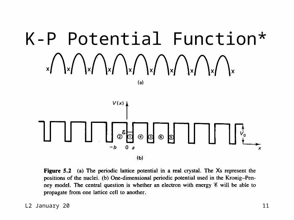
Kronig-Penney Model

A simple one-dimensional model of a crystalline solid

• V = 0, 0 < x < a, the ionic region

• V = Vo, a < x < (a + b) = L, between ions

• V(x+nL) = V(x), n = 0, +1, +2, +3, …,representing the symmetry of the assemblage of ions and requiring that (x+L) = (x) exp(jkL), Bloch’s Thm

L2 January 20 11

K-P Potential Function*

L2 January 20 12

K-P Static Wavefunctions• Inside the ions, 0 < x < a

(x) = A exp(jx) + B exp (-jx) = [82mE/h]1/2

• Between ions region, a < x < (a + b) = L (x) = C exp(x) + D exp (-x) = [82m(Vo-E)/h2]1/2

L2 January 20 13

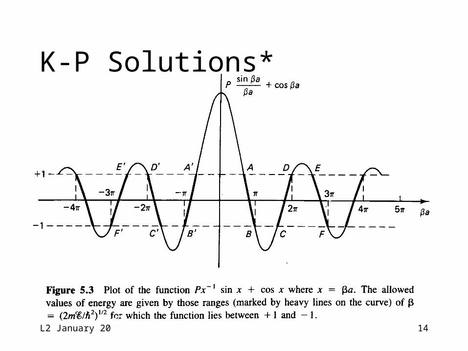
K-P Impulse Solution• Limiting case of Vo-> inf. and b -> 0,

while 2b = 2P/a is finite• In this way 2b2 = 2Pb/a < 1, giving

sinh(b) ~ b and cosh(b) ~ 1• The solution is expressed by

P sin(a)/(a) + cos(a) = cos(ka)• Allowed valued of LHS bounded by +1• k = free electron wave # = 2/

L2 January 20 14

K-P Solutions*

L2 January 20 15

K-P E(k) Relationship*

L2 January 20 16

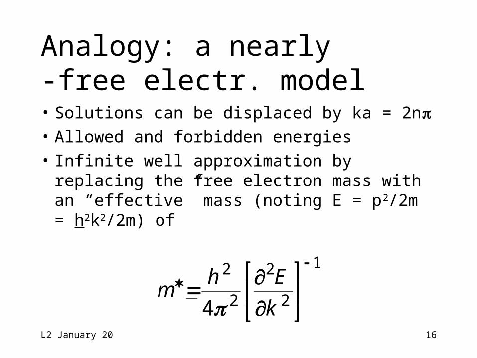
Analogy: a nearly-free electr. model• Solutions can be displaced by ka = 2n• Allowed and forbidden energies• Infinite well approximation by replacing

the free electron mass with an “effective” mass (noting E = p2/2m = h2k2/2m) of

1

2

2

2

2

4

k

Ehm

L2 January 20 17

Generalizationsand Conclusions

• The symm. of the crystal struct. gives “allowed” and “forbidden” energies (sim to pass- and stop-band)

• The curvature at band-edge (where k = (n+1)) gives an “effective” mass.

L2 January 20 18

Silicon Covalent Bond (2D Repr)

• Each Si atom has 4 nearest neighbors

• Si atom: 4 valence elec and 4+ ion core

• 8 bond sites / atom• All bond sites filled• Bonding electrons

shared 50/50_ = Bonding electron

L2 January 20 19

Silicon BandStructure**• Indirect Bandgap• Curvature (hence

m*) is function of direction and band. [100] is x-dir, [111] is cube diagonal

• Eg = 1.17-T2/(T+) = 4.73E-4 eV/K = 636K

L2 January 20 20

Si Energy BandStructure at 0 K

• Every valence site is occupied by an electron

• No electrons allowed in band gap

• No electrons with enough energy to populate the conduction band

L2 January 20 21

Si Bond ModelAbove Zero Kelvin

• Enough therm energy ~kT(k=8.62E-5eV/K) to break some bonds

• Free electron and broken bond separate

• One electron for every “hole” (absent electron of broken bond)

L2 January 20 22

Band Model forthermal carriers• Thermal energy

~kT generates electron-hole pairs

• At 300K Eg(Si) = 1.124 eV

>> kT = 25.86 meV,Nc = 2.8E19/cm3

> Nv = 1.04E19/cm3>> ni = 1.45E10/cm3

L2 January 20 23

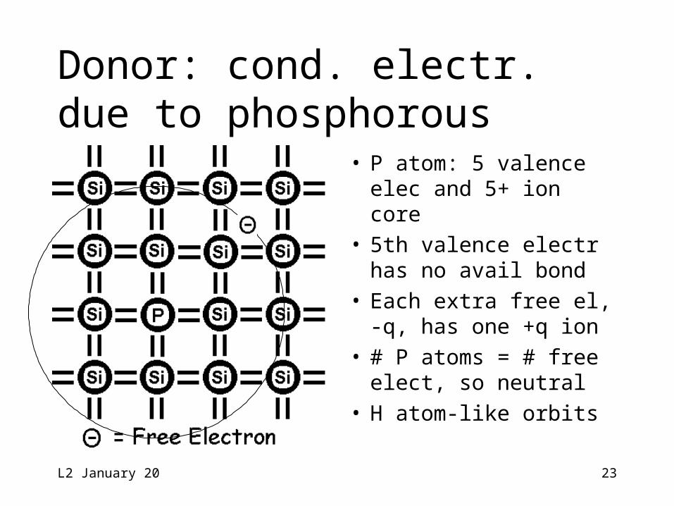
Donor: cond. electr.due to phosphorous

• P atom: 5 valence elec and 5+ ion core

• 5th valence electr has no avail bond

• Each extra free el, -q, has one +q ion

• # P atoms = # free elect, so neutral

• H atom-like orbits

L2 January 20 24

Bohr model H atom-like orbits at donor• Electron (-q) rev. around proton (+q)

• Coulomb force, F=q2/4Sio,q=1.6E-19 Coul, Si=11.7, o=8.854E-14 Fd/cm

• Quantization L = mvr = nh/2• En= -(Z2m*q4)/[8(oSi)2h2n2] ~-40meV

• rn= [n2(oSi)h2]/[Zm*q2] ~ 2 nm

for Z=1, m*~mo/2, n=1, ground state

L2 January 20 25

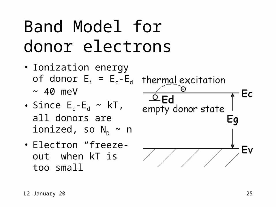
Band Model fordonor electrons• Ionization energy

of donor Ei = Ec-Ed ~ 40 meV

• Since Ec-Ed ~ kT, all donors are ionized, so ND ~ n

• Electron “freeze-out” when kT is too small

L2 January 20 26

Acceptor: Holedue to boron

• B atom: 3 valence elec and 3+ ion core

• 4th bond site has no avail el (=> hole)

• Each hole, adds --q, has one -q ion

• #B atoms = #holes, so neutral

• H atom-like orbits

L2 January 20 27

Hole orbits andacceptor states• Similar to free electrons and donor

sites, there are hole orbits at acceptor sites

• The ionization energy of these states is EA - EV ~ 40 meV, so NA ~ p and there is a hole “freeze-out” at low temperatures

L2 January 20 28

Impurity Levels in Si: EG = 1,124 meV• Phosphorous, P: EC - ED = 44 meV

• Arsenic, As: EC - ED = 49 meV

• Boron, B: EA - EV = 45 meV

• Aluminum, Al: EA - EV = 57 meV

• Gallium, Ga: EA - EV = 65meV

• Gold, Au: EA - EV = 584 meVEC - ED = 774 meV

L2 January 20 29

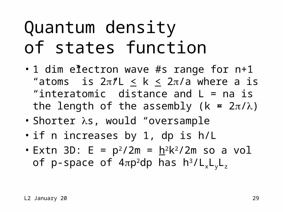
Quantum densityof states function• 1 dim electron wave #s range for n+1

“atoms” is 2/L < k < 2/a where a is “interatomic” distance and L = na is the length of the assembly (k = 2/)

• Shorter s, would “oversample”• if n increases by 1, dp is h/L• Extn 3D: E = p2/2m = h2k2/2m so a vol

of p-space of 4p2dp has h3/LxLyLz

L2 January 20 30

QM density of states (cont.)• So density of states, gc(E) is

(Vol in p-sp)/(Vol per state*V) =4p2dp/[(h3/LxLyLz)*V]

• Noting that p2 = 2mE, this becomes gc(E) = {42mn*)3/2/h3}(E-

Ec)1/2 and E - Ec = h2k2/2mn*

• Similar for the hole states whereEv - E = h2k2/2mp*

L2 January 20 31

Fermi-Diracdistribution fctn• The probability of an electron having

an energy, E, is given by the F-D distr fF(E) = {1+exp[(E-EF)/kT]}-1

• Note: fF (EF) = 1/2

• EF is the equilibrium energy of the system

• The sum of the hole probability and the electron probability is 1

L2 January 20 32

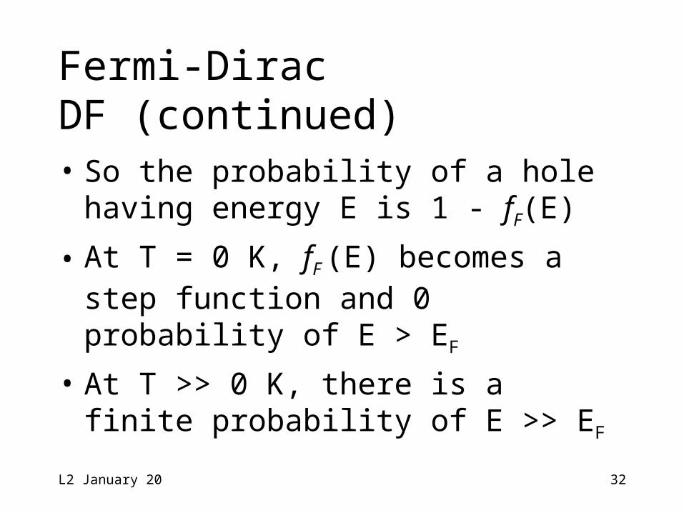
Fermi-DiracDF (continued)• So the probability of a hole having

energy E is 1 - fF(E)

• At T = 0 K, fF (E) becomes a step function and 0 probability of E > EF

• At T >> 0 K, there is a finite probability of E >> EF

L2 January 20 33

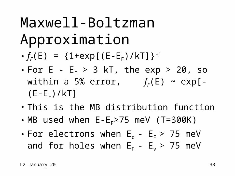
Maxwell-BoltzmanApproximation• fF(E) = {1+exp[(E-EF)/kT]}-1

• For E - EF > 3 kT, the exp > 20, so within a 5% error, fF(E) ~ exp[-(E-EF)/kT]

• This is the MB distribution function

• MB used when E-EF>75 meV (T=300K)

• For electrons when Ec - EF > 75 meV and for holes when EF - Ev > 75 meV

L2 January 20 34

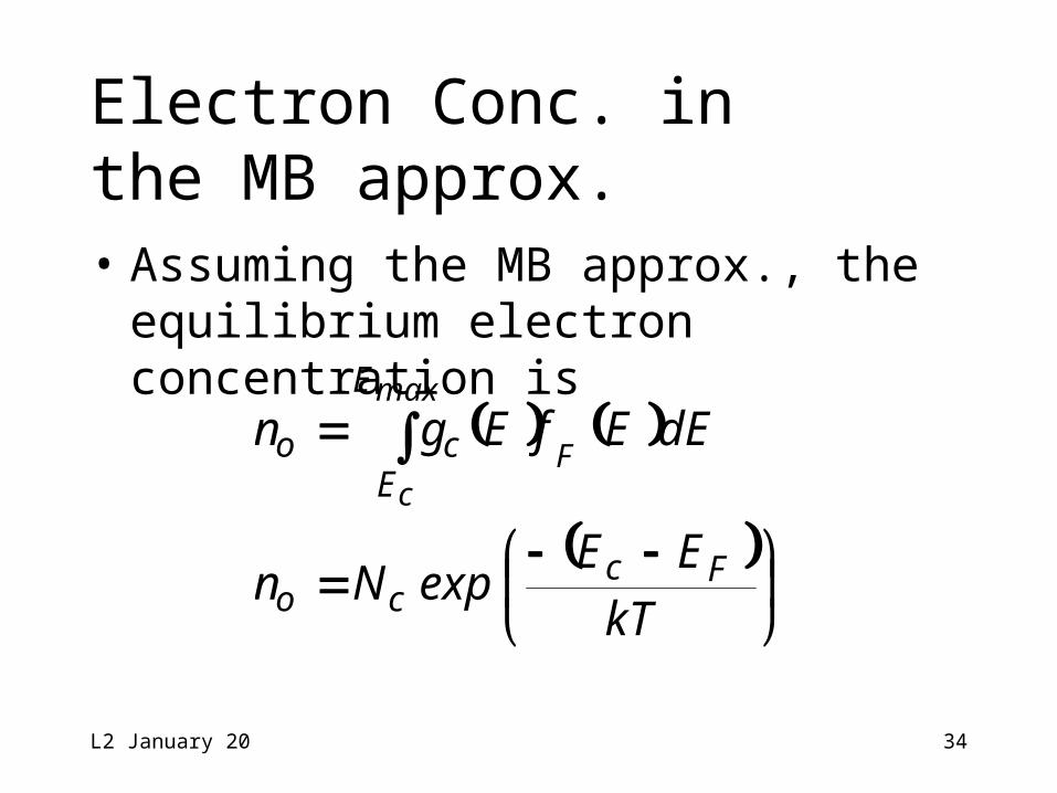
Electron Conc. inthe MB approx.• Assuming the MB approx., the

equilibrium electron concentration is

kTEE

expNn

dEEfEgn

Fcco

E

Eco F

max

c

L2 January 20 35

References

*Fundamentals of Semiconductor Theory and Device Physics, by Shyh Wang, Prentice Hall, 1989.

**Semiconductor Physics & Devices, by Donald A. Neamen, 2nd ed., Irwin, Chicago.

M&K = Device Electronics for Integrated Circuits, 3rd ed., by Richard S. Muller, Theodore I. Kamins, and Mansun Chan, John Wiley and Sons, New York, 2003.