AIAA 2000-1004

American Institute of Aeronautics and Astronautics

1

Abstract

A novel algorithm to generate hexahedral-dominant, semistructured grids is presented. The algorithm utilizes a parabolic marching scheme to generate the grid in structured layers starting from an initial data surface defined by a structured quadrilateral grid. A line deletion/insertion algorithm is applied at the interface between layers as the initial data surface for the next layer is being defined. Although the deletion/insertion algorithm used here is based solely on the geometric properties of the generated grid, it is not unique and great flexibility exists in how it is defined. The resulting grid topology offers a potentially attractive alternative to hexahedral and tetrahedral topologies for both interior and exterior grids. Several examples are included to demonstrate the efficacy of the approach.

Introduction

The solution of a discrete approximation to a field equation requires that a set of node points be developed on the boundaries and interior of the computational domain. The topology of the discrete set of points is typically classified in one of three ways: structured, unstructured, or hybrid. A grid defined using a set of hexahedral cells in which the connectivity of the points is implicitly defined by their ordering is classified as a structured grid. Structured grid topologies usually require the computational domain to be decomposed manually through the generation of blocks in which the structured grid is then generated. The effectiveness of utilizing systems of partial differential equations to generate structured grids is well documented.1-7 Elliptic, hyperbolic, and, to a lesser extent, parabolic systems have been used extensively to generate meshes for a wide variety of configurations. Parabolic methods are attractive because grids can be generated in times

comparable to those generated using hyperbolic methods but offer increased control of the point distribution, including the specification of points on the outer boundary.6,7 Algebraic methods have also been used extensively to generate grids for complex configurations.8,9

A grid defined using tetrahedral cells with an explicit, nontrivial connectivity table is categorized as an unstructured grid. Unstructured topologies are extremely flexible in that any volume can be filled with tetrahedra. Unstructured grids are generated in two processes: point creation and point connection.10-12 The most advanced automated grid generation systems for arbitrary geometries utilize unstructured grid topologies. However, unstructured grids potentially suffer from accuracy problems due to the skewness of high aspect ratio tetrahedra in viscous regions. Additionally, as reported by Shaw,13 there are concerns regarding the efficiency of the unstructured grid approach due to the large number of elements needed to discretize a given region. Hybrid grids are those grids that combine elements of structured and unstructured grids. Typically, prismatic or hexahedral cells are used in regions of the domain dominated by viscous effects.13-16 Away from viscous-dominated regions, tetrahedral or Cartesian grids are used. Hybrid topologies are unstructured in the sense that they require a complex connectivity table. They allow flexibility with respect to automation as well as feature resolution through the use of anisotropic elements. Typically, hybrid topologies require significantly fewer elements than unstructured grids to achieve the same resolution.13 It seems apparent that no single grid type can simultaneously address the conflicting requirements of solution accuracy, computational efficiency, and automation of the grid generation process. In this respect, hybrid grids appear to offer the most potential due to their flexibility. It is in this context that we define the unifying concept of the generalized grid topology. The generalized grid topology places no restriction on the number of edges

SEMISTRUCTURED GRID GENERATION IN THREE DIMENSIONS USING A PARABOLIC MARCHING SCHEME

D. S. Thompson* and B. K. Soni†

NSF/MSU Engineering Research Center Mississippi State University, Mississippi State, MS 39762

________ * Research Engineer, Member AIAA † Professor, Department of Aerospace Engineering, Senior Member AIAA Copyright © 2000 by the American Institute of Aeronautics and Astronautics, Inc. All rights reserved.

AIAA 2000-1004

American Institute of Aeronautics and Astronautics

2

used to define a face or the number of faces used to define a cell. The advantage of this type of grid is that grid elements may be used that are locally appropriate for the region being discretized. Here we define appropriate as simultaneously meeting the requirements of solution accuracy, computational efficiency, and automation of the grid generation process. Of course, there are performance penalties associated with CFD solvers utilizing the generalized grid topology when compared to codes developed for specific grid types. However, both the HYB3D code17 and the COBALT code18 have demonstrated the efficacy of generalized grid technology. All types of grids, with the exception of Chimera (overset) grids, are included within this framework.

In this paper, a novel algorithm to generate near-body, hexahedral-dominant, generalized grids is described.19 The algorithm uses a parabolic marching scheme coupled with a line deletion/insertion strategy to generate grids that have structure within each layer but lose connectivity at the interface between layers. The basics of the approach are discussed and the algorithm is demonstrated for several example configurations.

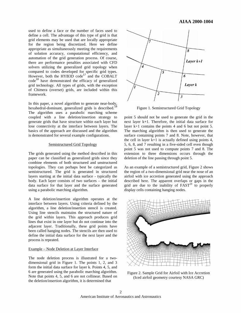
Semistructured Grid Topology The grids generated using the method described in this paper can be classified as generalized grids since they combine elements of both structured and unstructured topologies. They can perhaps best be categorized as semistructured. The grid is generated in structured layers starting at the initial data surface - typically the body. Each layer consists of two surfaces – the initial data surface for that layer and the surface generated using a parabolic marching algorithm. A line deletion/insertion algorithm operates at the interface between layers. Using criteria defined by the algorithm, a line deletion/insertion stencil is created. Using line stencils maintains the structured nature of the grid within layers. This approach produces grid lines that exist in one layer but do not continue into the adjacent layer. Traditionally, these grid points have been called hanging nodes. The stencils are then used to define the initial data surface for the next layer and the process is repeated. Example – Node Deletion at Layer Interface The node deletion process is illustrated for a two-dimensional grid in Figure 1. The points 1, 2, and 3 form the initial data surface for layer k. Points 4, 5, and 6 are generated using the parabolic marching algorithm. Note that points 4, 5, and 6 are not collinear. Based on the deletion/insertion algorithm, it is determined that

Figure 1. Semistructured Grid Topology

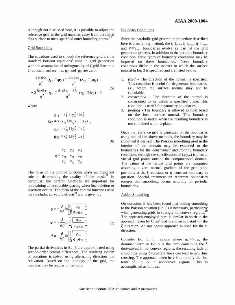
point 5 should not be used to generate the grid in the next layer k+1. Therefore, the initial data surface for layer k+1 contains the points 4 and 6 but not point 5. The marching algorithm is then used to generate the surface containing points 7 and 8. Note, however, that the cell in layer k+1 is actually defined using points 4, 5, 6, 8, and 7 resulting in a five-sided cell even though point 5 was not used to compute points 7 and 8. The extension to three dimensions occurs through the deletion of the line passing through point 5. As an example of a semistructured grid, Figure 2 shows the region of a two-dimensional grid near the nose of an airfoil with ice accretion generated using the approach described here. The apparent overlaps or gaps in the grid are due to the inability of FAST20 to properly display cells containing hanging nodes.

Figure 2. Sample Grid for Airfoil with Ice Accretion

(Iced airfoil geometry courtesy NASA GRC)

AIAA 2000-1004

American Institute of Aeronautics and Astronautics

3

Advantages of using the Semistructured Topology There are five main advantages to using a grid topology of this type for near-body grids: 1. Unlike unstructured grid topologies using

tetrahedral cells, it is possible to maintain large aspect ratio cells in viscous-dominated regions near no-slip boundaries resulting in accurate simulations in these regions and to easily transition to lower aspect ratio cells away from these regions.

2. Node deletion and insertion can result in a nearly isotropic face distribution for the pyramidal transition layer needed for the tetrahedral mesh generator resulting in a higher-quality tetrahedral mesh.

3. Higher-quality grids are obtained because lines can be inserted in regions of diverging grid lines, i.e., near convex corners.

4. Dense boundary point distributions may be used without the accompanying waste of grid points near the outer boundary that occurs with structured grid topologies. By using a line deletion/insertion algorithm based on cell aspect ratio, the points are deleted as the cell aspect ratio naturally decreases.

5. It is possible to develop a solution-adaptive grid strategy based on point redistribution and refinement. In addition to incorporating solution gradient information in the grid control functions, it is also possible to use solution information in the deletion/insertion algorithm.

The primary disadvantage of this grid topology is that the deletion/insertion actions affect the grid distribution throughout an entire layer. Additionally, only a limited number of flow solvers can utilize a grid of this type. Data Structure The key to efficiently implementing the semistructured grid topology is the data structure. The software developed by the authors is written in FORTRAN90 and makes extensive use of the derived data type and the dynamic memory allocation features of the language. The derived data type “ layer” consists of the information necessary to define each layer including the x, y, and z coordinates of the points on the initial data surface for the layer and the generated surface. Each layer is dynamically and independently dimensioned resulting in a highly efficient implementation.

Parabolic Grid Generation

In the parabolic method,5-7 a reference grid is utilized to make the marching problem well-posed. Starting from the initial data surface, two reference grid surfaces are

generated. The Poisson grid generation equations are applied to points on the first surface of the reference grid. This step is equivalent to smoothing the reference grid. The second surface is updated after each iteration of the Poisson grid equations. Note that the second surface of the reference grid is discarded once the desired number of smoothing iterations is complete. It should also be noted that the resulting smoothed grid still exhibits many of the characteristics of the reference grid. In practice, it has been found that reducing the grid point movement induced by the smoothing by two orders of magnitude results in a grid that is sufficiently smooth. Typically, this requires on the order of ten iterations of the alternating direction, line relaxation solver. Domains containing strongly non-convex regions require additional iteration. As is customary, a transformation of the form

(1) is defined and the inverse transformation

(2) is assumed to exist. The initial data surface is assumed to be defined by a ζ=constant surface and ζ is taken to be the marching direction. Reference Grid Definition The reference grid is generated algebraically to be locally orthogonal to the initial data surface for the layer. The first surface of the reference grid in layer k is defined using

(3) where ri,j,0 is the position vector to the point located at (i,j) on the initial data surface (0 subscript), ri,j,1 is the position vector to the point (i,j) on the first surface of the reference grid, δi,j is the specified distance distribution, and ni,j,0 is the unit surface normal. The second surface of the reference grid in layer k is generated using

(4)

kji

kji

kji

kji 1,,

1,1,,2,, nrr ++= δ

)z,y,x(

)z,y,x(

)z,y,x(

ζ=ζη=ηξ=ξ

),,(

),,(

),,(

ζηξζηξζηξ

zz

yy

xx

===

k0,j,i

kj,i

k0,j,i

k1,j,i nrr δ+=

AIAA 2000-1004

American Institute of Aeronautics and Astronautics

4

Although not discussed here, it is possible to adjust the reference grid as the grid marches away from the initial data surface to meet specified outer boundary points.6,7 Grid Smoothing The equations used to smooth the reference grid are the standard Poisson equations1 used in grid generation with the assumption of orthogonality of ζ grid lines to a ζ=constant surface, i.e., g13 and g23 are zero:

(5) where

(6)

The form of the control functions plays an important role in determining the quality of the mesh.19 In particular, the control functions are important for maintaining an acceptable spacing when line deletion or insertion occurs. The form of the control functions used here includes curvature effects21 and is given by

(7)

The partial derivatives in Eq. 5 are approximated using second-order central differences. The resulting system of equations is solved using alternating direction line relaxation. Based on the topology of the grid, the matrices may be regular or periodic.

Boundary Conditions Since the parabolic grid generation procedure described here is a marching method, the ξ=ξmin, ξ=ξmax, η=ηmin, and η=ηmax boundaries evolve as part of the grid generation process. In addition to the periodic boundary condition, three types of boundary conditions may be imposed on these boundaries. These boundary conditions differ in the manner in which the surface normal in Eq. 3 is specified and are listed below: 1. fixed - The direction of the normal is specified.

This condition is useful for degenerate boundaries, i.e., where the surface normal may not be calculable.

2. constrained - The direction of the normal is constrained to lie within a specified plane. This condition is useful for symmetry boundaries.

3. floating - The boundary is allowed to float based on the local surface normal. This boundary condition is useful when the resulting boundary is not contained within a plane.

Once the reference grid is generated on the boundaries using one of the above methods, the boundary may be smoothed if desired. The Poisson smoothing used in the interior of the domain may be extended to the boundaries for the constrained and floating boundary conditions through the specification of (x,y,z) triplets at virtual grid points outside the computational domain. The values at the virtual grid points are computed assuming a zero normal gradient of the grid point positions at the ξ=constant or η=constant boundary in question. Special treatment on reentrant boundaries ensures that smoothing occurs naturally for periodic boundaries. Added Smoothing On occasion, it has been found that adding smoothing to the Poisson equation (Eq. 5) is necessary, particularly when generating grids in strongly nonconvex regions.19 The approach employed here is similar in spirit to the approach taken by Chan3 and is shown in detail for the ξ direction. An analogous approach is used for the η direction. Consider Eq. 5. In regions where g11>>g33, the dominant term in Eq. 5 is the term containing the ζ derivatives. In nonconvex regions, the resulting lack of smoothing along ζ=constant lines can lead to grid line crossing. The approach taken here is to modify the first term of Eq. 5 in nonconvex regions. This is accomplished as follows:

∂∂−=

∂∂−=

∂∂−=

2211

33

3311

22

3322

11

ln

ln

ln

gg

g

gg

g

gg

g

ζθ

ηψ

ξφ

0)(g

ggg

g

gg2

)(g

gg)(

g

gg

2

2122211

23312

23311

23322

=θ+−

+−

ψ++φ+

ζζζξη

ηηηξξξ

rrr

rrrr

ζζζ

ηηη

ξξξ

ζζζ

ηηη

ηξηξηξ

ξξξ

=

++=

++=

++=

++=

zyx

zyx

zyx

g

zyxg

zyxg

zzyyxxg

zyxg

22233

22222

12

22211

AIAA 2000-1004

American Institute of Aeronautics and Astronautics

5

(8)

where

(9)

θξ is the angle between ri+1,j-ri,j and ri-1,j-ri,j and 0<α<1 is a user-specified parameter that controls the amount of smoothing in mildly-concave regions. Smaller values of α result in more smoothing. Note that no additional smoothing is added in convex regions.

Line Deletion/Insertion Algorithm The line deletion/insertion algorithm employed here is based solely on geometrical properties of the grid. The procedure used for ξ line deletion will be presented in detail with the extension to η lines by analogy. It is assumed there are jmax points located on each ξ line. There is great flexibility in the design of the deletion/insertion algorithm and the strategy discussed below is certainly not unique. Although not demonstrated here, it is possible to define insertion and deletion algorithms based on flow field properties as well. Line Deletion/Insertion Strategy An ξ line is tagged for deletion if it meets either of two criteria. The first criterion is based on the average “slenderness” of the cells on an ξ=constant line. An ξ=constant line is marked for deletion if the average value of the ratio of the ξ arc length to the ζ arc length is greater than a specified tolerance or

(10) where jmax is the number of points on each ξ=constant line. The second criterion is based on a maximum “slenderness” of the cells on each ξ line. An ξ=constant

line is marked for deletion if the value of the ratio of the ξ arc length to the ζ arc length is greater than a specified tolerance at any point on the line or

(11) Note that αavg and αmax are user-specified constants with αmax > αavg .

Since the criteria described in Eq. 10 and Eq. 11 are defined on a line-by-line basis without any information regarding adjacent lines, it is necessary to determine the deletion/insertion stencil incorporating the information from adjacent lines. The first step is tagging contiguous groups of ξ lines that are selected for deletion and identifying whether the groups contain an even number or an odd number of elements. In the case of an odd number of contiguous ξ lines selected for deletion, the first line of the group, and every other succeeding line of the group, are deleted. The case of a single line selected for deletion is trivial. The case of an even number of contiguous ξ lines selected for deletion is treated using a delete two/insert one strategy. For each consecutive pair of lines tagged for deletion, both are deleted and replaced by the line defined by connecting the midpoints between the two lines tagged for deletion. Line Insertion Strategy The criteria used to determine if an ξ=constant line should be inserted is based on the divergence of the ξ=constant faces of the cell. Unlike the deletion criteria, the insertion criteria apply to a cell face rather than a line. Here, the divergence of the cell is defined as

(12) As for the line deletion algorithm, average and maximum values of the divergence are used in the algorithm. A surface of ξ=constant and ζ=constant cell faces is tagged for ξ line insertion if the average divergence exceeds a specified tolerance

(13)

))1((2

3322ξξξξ φν rr ++

g

gg

( )ξξ θν fg

gg ×=33

3311 ),(max

( ) ( )

î

θ≤π

π<θ≤πθ

π<θ≤

=θ

ξ

ξα

ξ

ξ

ξ

02

sin

201

f

avg

j

j

j g

g

jα>

∑=

max

1 11

33

max

1

max11

33max α>

jj g

g

( )1133

gg

1

ζ∂∂=∆

( ) avg

maxj

1jj

maxj

1 β>∆∑=

AIAA 2000-1004

American Institute of Aeronautics and Astronautics

6

Similarly, a surface of ξ=constant and ζ=constant cell faces is tagged for ξ line insertion if the maximum divergence exceeds a specified tolerance

(14) where βmax > βavg. The line insertion occurs at the midpoints of the cell faces. Cell Topology The line deletion/insertion scheme described above produces cell edges having one, two, or three segments. The cell faces can have four to seven edges and the resulting volumes may have 6 to 17 faces. However, for viscous-type grids in particular, a majority of the cells (typically greater than 95%) are hexahedra. It should be noted that other deletion/insertion schemes will produce different cell topologies.

Sample Grids Included here are five grids generated using the parabolic marching scheme with line deletion/insertion. For all cases shown here, the grids were generated using αavg = 1.5 and αmax = 2. In cases where line insertion was used, βavg = 0.2 and βmax = 0.3. The marching distance distribution, δk, generated using a hyperbolic tangent stretching function and was taken to be constant in each layer and. The grids were generated using a relatively small number of points for improved visual clarity. The figures shown here were generated using FAST.20 The data were saved in a format that FAST could process by defining adjacent layers with no deletion or insertion as a zone. Again, the overlaps or gaps in the grid are due to the inability of FAST to properly display cells containing hanging nodes. Simple Bump Three views of a grid generated for a simple bump configuration are shown in Figures 3, 4, and 5. The height of the bump was defined using the product of two cosine functions inside a specified radius and set to zero outside the specified radius. The initial surface grid dimensions were 31x21. In the tenth and final layer, the grid dimensions were 19x13. There were 4388 total cells. The floating condition was used for each of the boundaries. This case illustrates the topology of the grid as well as the effects of line deletion. As can be seen from the figures, the grid transitions are smooth and the grid appears to be of high quality. The effects of the normal gradient boundary

Figure 3. Simple bump grid – y=constant plane

Figure 4. Simple bump grid – ξ=1, η=1,

ζ=1, and ζ=ζmax surfaces

Figure 5. Simple bump grid – Comparison of ζ=1 and ζ=ζmax surfaces

( ) maxjj

max β>∆

AIAA 2000-1004

American Institute of Aeronautics and Astronautics

7

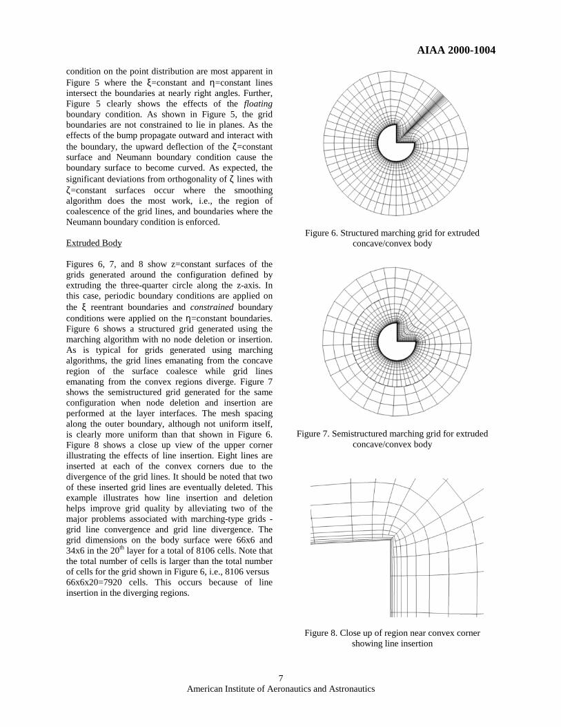
condition on the point distribution are most apparent in Figure 5 where the ξ=constant and η=constant lines intersect the boundaries at nearly right angles. Further, Figure 5 clearly shows the effects of the floating boundary condition. As shown in Figure 5, the grid boundaries are not constrained to lie in planes. As the effects of the bump propagate outward and interact with the boundary, the upward deflection of the ζ=constant surface and Neumann boundary condition cause the boundary surface to become curved. As expected, the significant deviations from orthogonality of ζ lines with ζ=constant surfaces occur where the smoothing algorithm does the most work, i.e., the region of coalescence of the grid lines, and boundaries where the Neumann boundary condition is enforced. Extruded Body Figures 6, 7, and 8 show z=constant surfaces of the grids generated around the configuration defined by extruding the three-quarter circle along the z-axis. In this case, periodic boundary conditions are applied on the ξ reentrant boundaries and constrained boundary conditions were applied on the η=constant boundaries. Figure 6 shows a structured grid generated using the marching algorithm with no node deletion or insertion. As is typical for grids generated using marching algorithms, the grid lines emanating from the concave region of the surface coalesce while grid lines emanating from the convex regions diverge. Figure 7 shows the semistructured grid generated for the same configuration when node deletion and insertion are performed at the layer interfaces. The mesh spacing along the outer boundary, although not uniform itself, is clearly more uniform than that shown in Figure 6. Figure 8 shows a close up view of the upper corner illustrating the effects of line insertion. Eight lines are inserted at each of the convex corners due to the divergence of the grid lines. It should be noted that two of these inserted grid lines are eventually deleted. This example illustrates how line insertion and deletion helps improve grid quality by alleviating two of the major problems associated with marching-type grids - grid line convergence and grid line divergence. The grid dimensions on the body surface were 66x6 and 34x6 in the 20th layer for a total of 8106 cells. Note that the total number of cells is larger than the total number of cells for the grid shown in Figure 6, i.e., 8106 versus 66x6x20=7920 cells. This occurs because of line insertion in the diverging regions.

Figure 6. Structured marching grid for extruded

concave/convex body

Figure 7. Semistructured marching grid for extruded

concave/convex body

Figure 8. Close up of region near convex corner

showing line insertion

AIAA 2000-1004

American Institute of Aeronautics and Astronautics

8

Figure 9. Grid generated around body of revolution

Figure 10. Detail of nonconvex region near nozzle

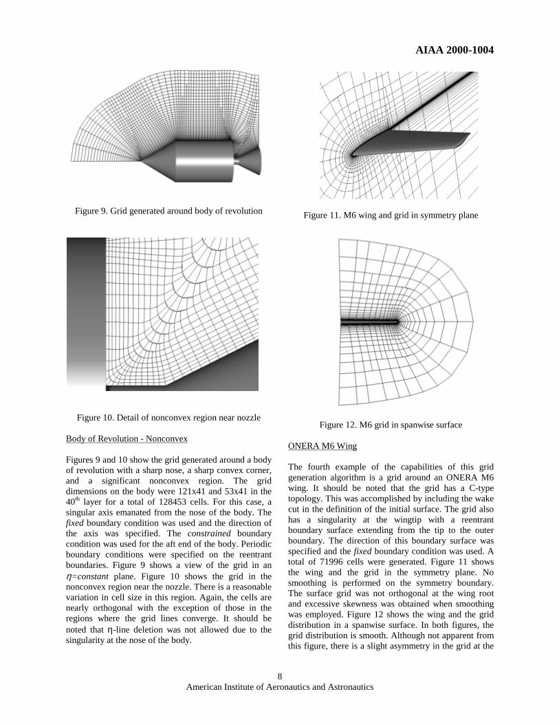
Body of Revolution - Nonconvex Figures 9 and 10 show the grid generated around a body of revolution with a sharp nose, a sharp convex corner, and a significant nonconvex region. The grid dimensions on the body were 121x41 and 53x41 in the 40th layer for a total of 128453 cells. For this case, a singular axis emanated from the nose of the body. The fixed boundary condition was used and the direction of the axis was specified. The constrained boundary condition was used for the aft end of the body. Periodic boundary conditions were specified on the reentrant boundaries. Figure 9 shows a view of the grid in an η=constant plane. Figure 10 shows the grid in the nonconvex region near the nozzle. There is a reasonable variation in cell size in this region. Again, the cells are nearly orthogonal with the exception of those in the regions where the grid lines converge. It should be noted that η-line deletion was not allowed due to the singularity at the nose of the body.

Figure 11. M6 wing and grid in symmetry plane

Figure 12. M6 grid in spanwise surface

ONERA M6 Wing The fourth example of the capabilities of this grid generation algorithm is a grid around an ONERA M6 wing. It should be noted that the grid has a C-type topology. This was accomplished by including the wake cut in the definition of the initial surface. The grid also has a singularity at the wingtip with a reentrant boundary surface extending from the tip to the outer boundary. The direction of this boundary surface was specified and the fixed boundary condition was used. A total of 71996 cells were generated. Figure 11 shows the wing and the grid in the symmetry plane. No smoothing is performed on the symmetry boundary. The surface grid was not orthogonal at the wing root and excessive skewness was obtained when smoothing was employed. Figure 12 shows the wing and the grid distribution in a spanwise surface. In both figures, the grid distribution is smooth. Although not apparent from this figure, there is a slight asymmetry in the grid at the

AIAA 2000-1004

American Institute of Aeronautics and Astronautics

9

wing tip in Figure 12. Through line deletion/insertion, this asymmetry is propagated back to the symmetry plane. The grid dimensions on the initial surface were 97x17. In the 60th and final layer, the grid dimensions were 27x8. The surface shown in Figure 12 is a truly three-dimensional surface and is shown in perspective. “X-38-Like” Body The final example shown here is a grid generated around a body similar to the X-38 Crew Return Vehicle. The initial surface dimensions were 59x100. There is a singular axis at the nose that was treated by specifying its direction and using the fixed condition. At the aft end of the body, the floating boundary condition was applied. The dimensions in the 10th and final layer were 25x41. There were 44979 total cells. Limiting the ξ-range of the deletion/insertion algorithm so that the region near the singular axis was avoided facilitated deletion of lines in the periodic direction. Figures 13, 14, and 15 show different views of the grid. Again, the grid shows smooth transitions and is of high quality. The grid is mostly orthogonal and does not exhibit the coalescence/divergence of grid lines characteristic of marching methods. Although not apparent from the figures, grid lines were inserted near the wing tips to improve the grid quality in these strongly convex regions. With the exception of the region near the singular axis emanating from the nose, the outer boundary of the grid exhibits a relatively isotropic distribution of the cell size.

Observations

At this point, it is appropriate to review the characteristics of the semistructured grid generation algorithm. 1. The algorithm appears capable of generating high-

quality, near-body grids for generalized grid applications.

2. The initial surface definition must consist of a structured, quadrilateral grid. Other surface mesh topologies have not been addressed at this time. It may be possible to relax this requirement and use triangular or unstructured quadrilateral surface meshes and a generalized smoothing algorithm.22 We are currently investigating this approach.

3. The quality of the volume grid is dependent on the quality of the surface grid. Of course, this result is not unique to this algorithm and is true for any marching or advancing front algorithm.

4. The global nature of deletion/insertion algorithm within each layer is necessary to maintain structured layers. Since mesh characteristics can vary dramatically along a coordinate line, it is

Figure 13. Grid at downstream boundary of domain

Figure 14. Symmetry plane of grid

Figure 15. Outer boundary of grid

AIAA 2000-1004

American Institute of Aeronautics and Astronautics

10

possible to delete/insert lines based on a local geometric anomaly.

5. Although not demonstrated here, the flexibility offered by the insert/deletion algorithm facilitates the possibility of grid adaptation based on solution gradients using refinement and point redistribution.

Summary

The capability to generate semistructured, three-dimensional, hexahedral-dominant grids has been demonstrated. The method was shown to generate quality volume grids for surfaces with concave and convex regions. The parabolic marching method generates the grid in structured layers. First, an orthogonal reference grid is generated using an algebraic approach. The reference grid is then smoothed using the standard Poisson grid generation equations. Using the Poisson equations to smooth the grid point locations provides improved control over grid point placement through the control functions. Although each layer is structured, this structure may be lost at the interface between layers upon application of the line deletion/insertion algorithm. A deletion/insertion algorithm based on cell aspect ratio and grid line divergence has been demonstrated. This strategy is not unique and great flexibility exists in the definition of the deletion/insertion algorithm. Finally, the efficacy of the approach was demonstrated by generating grids for several example configurations.

References 1. J. F. Thompson, “A General Three-Dimensional

Elliptic Grid Generation System on a Composite Block Structure,” Comp. Meth. App. Mech. Eng., Vol. 64, pp. 377-411, 1987.

2. S. P. Spekreijse, “Elliptic Grid Generation Based on Laplace Equations and Algebraic Transformations,” J. Comp. Phys.,Vol. 118, pp. 38-61, 1995.

3. W. M. Chan and J. L. Steger, “Enhancements of a Three-Dimensional Hyperbolic Grid Generation Scheme,” Appl. Math. Comput., Vol. 51, pp.181-205, 1992.

4. J. A. Bacon, T. L. Henderson, and K. D. Lee, “Grid Generation using an Elliptic-Hyperbolic Hybrid Method,” Numerical Grid Generation in Computational Fluid Dynamics and Related Fields, Eds. N. Weatherill, P. R. Eiseman, J. Hauser, and J. F. Thompson, Pineridge Press Ltd., Swansea, U.K, pp. 3-14, 1994.

5. S. Nakamura, “Marching Grid Generation Using Parabolic Partial Differential Equations,” Numerical Grid Generation, Ed. J. F. Thompson,

Elsevier Science Publishing Company, Inc., New York, pp. 775-786, 1982.

6. R. W. Noack and D. A. Anderson, “Solution-Adaptive Grid Generation using Parabolic Partial Differential Equations,” AIAA J., Vol. 28, pp.1016-1023, 1990.

7. R. W. Noack, and I. H. Parpia, “Solution Adaptive Parabolic Grid Generation in Two and Three Dimensions,” Numerical Grid Generation in Computational Fluid Dynamics and Related Fields, Eds. A. S.-Arcilla, J. Hauser, P. R. Eiseman, and J. F. Thompson, Elsevier Science Publishing Company, New York, pp. 475-484, 1991.

8. R. E. Smith, “Transfinite Interpolation (TFI) Generation Systems,” Handbook of Grid Generation, Eds. J. F Thompson, B. K. Soni, and N. P. Weatherill, CRC Press, Boca Raton, FL, 1998.

9. T.-Y. Yu and B. K. Soni, “The Application of NURBS in Numerical Grid Generation,” J. Comput. Aided Design, Vol. 27, pp. 147-157, 1995.

10. N. P. Weatherill, “A Method for Generating Irregular Computational Grids in Multiply Connected Planar Domains,” Int. J. Num. Methods Fluids, Vol. 8, pp. 181-197, 1988.

11. N. P. Weatherill and O. Hassan, “Efficient Three-Dimensional Delaunay Triangulation with Automatic Point Creation and Imposed Boundary Constraints,” Int. J. Num. Methods Eng., Vol. 37, 1994, pp. 2005-2039.

12. D. L. Marcum and N. P. Weatherill, “Unstructured Grid Generation Using Iterative Point Insertion and Local Reconnection,” AIAA J., Vol. 33, p. 1619-1625, 1995.

13. J. A. Shaw, “Hybrid Grids,” Handbook of Grid Generation, Eds. J. F Thompson, B. K. Soni, and N. P. Weatherill, CRC Press, Boca Raton, FL, 1998.

14. J. A. Chappell, J. A. Shaw, M. Leatham, “The Generation of Hybrid Grids Incorporating Prismatic Regions for Viscous Flow Calculations,” Numerical Grid Generation in Computational Field Simulation, Eds. M. Cross, B. K. Soni, J. F. Thompson, J. Hauser, and P. R. Eiseman, NSF Engineering Research Center for Computational Field Simulations, Mississippi State, MS, pp. 537-546, 1996.

15. Y. Kallinderis, “Hybrid Grids and Their Applications,” Handbook of Grid Generation, Eds. J. F Thompson, B. K. Soni, and N. P. Weatherill, CRC Press, Boca Raton, FL, 1998.

16. C.-T. Huang, “Hybrid Grid Generation System,” M.S. Thesis, Department of Aerospace Engineering, Mississippi State University, 1996.

AIAA 2000-1004

American Institute of Aeronautics and Astronautics

11

17. R. P. Koomullil and B. K. Soni, “Generalized Grid Techniques in Computational Field Simulation,” Numerical Grid Generation in Computational Field Simulations, Eds. M. Cross, P. R. Eiseman, J. Hauser, B. K. Soni, and J. F. Thompson, International Society for Grid Generation, Mississippi State, MS, pp. 521-531,1998.

18. R. F. Tomaro, W. Z. Strang, and L. N. Sankar, “An Implicit Algorithm for Solving Time Dependent Flows on Unstructured Grids,” AIAA Paper 97-0333, Presented at 35th Aerospace Sciences Meeting, Reno, NV, January 1997.

19. D. S. Thompson and B. K. Soni, “Generation of Quad- and Hex-Dominant, Semistructured Grids using an Advancing Layer Scheme,” Proc. 8th Int. Meshing Roundtable 1999, Sandia National Laboratories, pp. 171-178, 1999.

20. “FAST User Guide.” <http://www.nas.nasa.gov/ Software/FAST/>, June, 1999.

21. B. K. Soni, “Elliptic Grid Generation Systems: Control Functions Revisited,” App. Math. Comp., Vol. 59, pp. 151-164, 1993.

22. P. M. Knupp, “Winslow Smoothing on Two-Dimensional Unstructured Meshes,” Proc. 7th Int. Meshing Roundtable ‘98, Sandia National Laboratories, pp. 449-457, 1998.