R E S E A R CH A R T I C L E

Sensitivity analysis and uncertainty assessment in waterbudgets simulated by the variable infiltration capacity modelfor Canadian subarctic watersheds

Rajtantra Lilhare1 | Scott Pokorny2 | Stephen J. Déry2,3 |

Tricia A. Stadnyk2,3,4 | Kristina A. Koenig5

1Natural Resources and Environmental Studies

Program, University of Northern British

Columbia, Prince George, British Columbia,

Canada

2Department of Civil Engineering, University

of Manitoba, Winnipeg, Manitoba, Canada

3Environmental Science and Engineering

Program, University of Northern British

Columbia, Prince George, British Columbia,

Canada

4Department of Geography, University of

Calgary, Calgary, Alberta, Canada

5Water Resources Engineering Department,

Manitoba Hydro, Winnipeg, Manitoba, Canada

Correspondence

Rajtantra Lilhare, Natural Resources and

Environmental Studies Program, University of

Northern British Columbia, Prince George,

British Columbia, Canada.

Email: lilhare@unbc.ca

Funding information

Natural Sciences and Engineering Research

Council of Canada, Grant/Award Number:

NSERC CRD 44425 RC15-3100; Manitoba

Hydro

Abstract

In this study, we evaluate uncertainties propagated through different climate data

sets in seasonal and annual hydrological simulations over 10 subarctic watersheds of

northern Manitoba, Canada, using the variable infiltration capacity (VIC) model. Fur-

ther, we perform a comprehensive sensitivity and uncertainty analysis of the VIC

model using a robust and state-of-the-art approach. The VIC model simulations uti-

lize the recently developed variogram analysis of response surfaces (VARS) technique

that requires in this application more than 6,000 model simulations for a 30-year

(1981–2010) study period. The method seeks parameter sensitivity, identifies influ-

ential parameters, and showcases streamflow sensitivity to parameter uncertainty at

seasonal and annual timescales. Results suggest that the Ensemble VIC simulations

match observed streamflow closest, whereas global reanalysis products yield high

flows (0.5–3.0 mm day−1) against observations and an overestimation (10–60%) in

seasonal and annual water balance terms. VIC parameters exhibit seasonal impor-

tance in VARS, and the choice of input data and performance metrics substantially

affect sensitivity analysis. Uncertainty propagation due to input forcing selection in

each water balance term (i.e., total runoff, soil moisture, and evapotranspiration) is

examined separately to show both time and space dimensionality in available forcing

data at seasonal and annual timescales. Reliable input forcing, the most influential

model parameters, and the uncertainty envelope in streamflow prediction are pres-

ented for the VIC model. These results, along with some specific recommendations,

are expected to assist the broader VIC modelling community and other users of

VARS and land surface schemes, to enhance their modelling applications.

K E YWORD S

hydrological modelling, lower Nelson River basin, sensitivity analysis, uncertainty assessment,

VARS, VIC model, VIC parameters, water balance

1 | INTRODUCTION

Numerical modelling of a river basin remains essential for both climate

and ecological studies as it provides vital information about the

hydrological cycle and water availability for societies and ecosystems.

Although recent developments and advances have been achieved in

hydrological modelling and computational power, addressing effi-

ciently the uncertainties in hydrological simulation remains a critical

Received: 18 September 2019 Accepted: 21 January 2020

DOI: 10.1002/hyp.13711

Hydrological Processes. 2020;34:2057–2075. wileyonlinelibrary.com/journal/hyp © 2020 John Wiley & Sons Ltd 2057

challenge (Liu & Gupta, 2007). There is a growing need for sensitivity

and uncertainty assessments associated mainly with the model and

input forcing data sets to achieve the hydrological model's optimal

performance for decision-making. Input climate forcing for numerical

modelling, primarily precipitation and air temperature, are essential for

accurate streamflow simulations and water balance calculations (Eum,

Dibike, Prowse, & Bonsal, 2014; Fekete, Vörösmarty, Roads, &

Willmott, 2004; Reed et al., 2004; Tobin, Nicotina, Parlange, Berne, &

Rinaldo, 2011). For cold regions, these input forcing alter the phase

and magnitude of modelled variables and cascade through all hydro-

logical processes during numerical simulations, impacting the reliability

of model output (Anderson et al., 2008; Tapiador et al., 2012;

Wagener & Gupta, 2005). In Canada, however, numerous studies have

also used multiple forcing data sets to assess the performance of

hydrological simulations. For example, Sabarly, Essou, Lucas-Picher,

Poulin, and Brissette (2016) used four reanalysis products to evaluate

the terrestrial branch of the water cycle over Québec, Canada with

acceptable results for the period 1979–2008. The question of which

forcing data set is the most suitable and accurate to drive hydrological

models remains elusive and inconclusive. Steps towards answering

that question were undertaken by Pavelsky and Smith (2006) who

concluded that observations covered the trends significantly better

than two reanalysis products when they assessed the quality of four

global precipitation data sets against the discharge observations from

198 pan-Arctic rivers. The bias and uncertainty in global hydrological

modelling due to input data sets and associated overestimations or

underestimations in modelled streamflows in several river basins have

also been identified in previous studies (e.g., Döll, Kaspar, & Lehner,

2003; Gerten, Schaphoff, Haberlandt, Lucht, & Sitch, 2004; Nijssen,

Schnur, & Lettenmaier, 2001). Although there may be other uncer-

tainties (e.g., model structure, calibration, soil type, land use, etc.), this

paper focuses primarily on the uncertainties due to model parameters

and input forcing data sets, which are perhaps the most significant

source of uncertainty for any hydrological modelling study (Zhang, Li,

Huang, Wang, & Cheng, 2016).

In practice, many (from tens to hundreds) parameters in most

hydrological models lead to dimensionality issues where parameter

estimation becomes mostly nonlinear and a high-dimensional problem.

Numerous optimization algorithms are available to address these

problems (e.g., Abebe, Ogden, & Pradhan, 2010; Aster, Borchers, &

Thurber, 2013; Beven & Binley, 1992; Duan, Sorooshian, & Gupta,

1992; Hill & Tiedeman, 2007; Vrugt, Diks, Gupta, Bouten, & Ver-

straten, 2005; Vrugt, Gupta, Bouten, & Sorooshian, 2003), but it is not

often feasible or necessary to include all these parameters in the cali-

bration and sensitivity analysis (SA) process to obtain efficient optimi-

zation and sensitive parameters, respectively. For instance, over-

parameterization is another well-known problem in land surface

modelling (Van Griensven et al., 2006). At present, various SA

methods (e.g., qualitative or quantitative, local or global, and screening

or refined methods) are used widely in different fields, such as com-

plex engineering systems, physics, and social sciences (Frey & Patil,

2002; Iman & Helton, 1988). Given the extensive range of SA

methods available, users should have a clear understanding of the

methods that are appropriate for a specific application. In general, the

variable infiltration capacity (VIC) hydrological model incorporates

many parameters (some with physical significance and some statisti-

cal), which are used to calibrate the model by various methods. In

some cases, parameters with physical significance may be adjusted

interactively during calibration. Some parameters may have less influ-

ence on model output such that they could be easily ignored. One of

the objectives of this study is thus to explore the sensitivity of VIC

calibration parameters to reduce the dimensionality issue in model

optimization at different timescales and to establish their interannual

importance in the calibration and model performance.

In this study, we quantify the uncertainty propagated from avail-

able forcing data sets in their surface water balance estimations over

the lower Nelson River Basin (LNRB) in northern Manitoba, Canada.

To achieve this goal, seven input forcing data sets that are inter-

compared in our companion paper are ingested into the VIC model

over the LNRB (Lilhare, Déry, Pokorny, Stadnyk, & Koenig, 2019).

These data sets are used in various other studies over different Cana-

dian regions (Boucher & Best, 2010; Islam & Déry, 2017; Sauchyn,

Vanstone, & Perez-Valdivia, 2011; Seager et al., 2014; Woo & Thorne,

2006). To our knowledge, this is perhaps the first comprehensive

study that collectively utilizes available gridded data sets in hydrologi-

cal modelling, establishes the most suitable data sets, minimizes the

input data uncertainty by evaluating the best performing product, and

then propagates input and parameter uncertainty through the model

output. Moreover, we consider not only the total uncertainty

(i.e., total run-off) but also the apportioned uncertainty in run-off-

generating processes such as precipitation, evapotranspiration

(ET hereafter), and soil moisture at annual and seasonal timescales.

The main objectives of this study are to (a) examine uncertainty prop-

agated through various input forcing data sets in the VIC model;

(b) identify parameter sensitivity of the VIC model to streamflow; and

(c) assess streamflow sensitivity to parameter uncertainty in the VIC

model over the LNRB.

2 | STUDY AREA

In this study, the lower Nelson River, which is the downstream seg-

ment of the Nelson River system, is selected for the VIC modelling,

sensitivity, and uncertainty analyses (Figure 1). The LNRB spans an

area of ~90,500 km2 and collects all water from the drainage area

upstream of the Nelson River (~970,000 km2) before discharging into

Hudson Bay. In the LNRB, the main stem river (Nelson) and its largest

tributary—the Burntwood, whose downstream segment carries diver-

ted flows from the Churchill River—have less seasonal flow variability

due to streamflow regulation and a large drainage area. Most of the

LNRB has gentle slopes, with common channelized lakes moderating

flow variability. Wetlands abound within the LNRB, store significant

volumes of water, cover large areas, and moderate streamflow

responses to rainfall and snowmelt events. Shallow soils and perma-

frost limit infiltration, groundwater storage, and groundwater flows.

To increase its hydroelectric capacity, Manitoba Hydro manages flows

2058 LILHARE ET AL.

in the LNRB with two major sources of streamflow regulation: the

Churchill River diversion and Lake Winnipeg regulation.

The LNRB experiences a subarctic continental climate character-

ized by moderate precipitation and humidity, cool summers, and cold

winters. The snow-free season remains brief, generally beginning in

May and ending in October. Most of the precipitation that occurs dur-

ing the summer months falls as rain, accounting nearly two-thirds of

the total annual precipitation. The most expansive land cover class in

the LNRB is temperate or subpolar needleleaf forest covering ~33%

of its total area with secondary classes being mixed forests (19%) and

temperate or subpolar shrublands (9%; North American Land Change

Monitoring System, 2010). Wetlands (bogs and fens, 21%) and open

surface water (13%) also prevail in the region. The entire region

exhibits low relief with a maximum elevation of 390 m a.s.l. and aver-

age basin slope of 0.037%. Permafrost abounds in the LNRB with the

downstream, northeastern portion underlain by continuous (between

90% to 100%) and extensive discontinuous (between 50% to 90%)

permafrost (approximately 0.8% and 9% of the LNRB, respectively),

whereas sporadic discontinuous (between 10% to 50%) and isolated

permafrost spans ~68% and 16% of the LNRB's total area, respec-

tively (Natural Resources Canada, 2010).

3 | MATERIALS AND METHODS

3.1 | Data sets

Soil parameters for the VIC model are sourced from the multi-

institution North American Land Data Assimilation System project at

0.50� resolution (Cosby, Hornberger, Clapp, & Ginn, 1984). These soil

parameters are then aggregated to the VIC model resolution (0.10�)

following Mao and Cherkauer (2009). Frost-related parameters

(e.g., bubbling pressure) are extracted from Miller and White (1998) or

set to default values (Mao & Cherkauer, 2009). Land cover data are

obtained from the Natural Resources Canada's GeoGratis–Land

Cover, and circa 2000-Vector product and vegetation parameters are

estimated by following Sheffield and Wood (2007). All land cover clas-

ses are mapped into standard VIC model vegetation classes, and the

leaf area index for each vegetation class in every grid cell is estimated

(Myneni, Ramakrishna, Nemani, & Running, 1997). Rooting depths are

obtained from Maurer, Wood, Adam, Lettenmaier, and Nijssen (2002),

whereas other vegetation parameters are taken from Nijssen

et al. (2001).

We obtain various gridded forcing data sets for further analysis:

the Australian National University spline interpolation (ANUSPLIN),

North American Regional Reanalysis (NARR), European Centre for

Medium-Range Weather Forecasts interim reanalysis (ERA-Interim),

European Union Water and Global Change (WATCH) Forcing Data

ERA-Interim (WFDEI), and Hydrological Global Forcing Data

(HydroGFD). As well, an inverse distance weighted (IDW) data set

constructed from 14 Environment and Climate Change Canada mete-

orological stations across the LNRB using a squared IDW interpolation

technique is also used (see Table 1 for more details). These data sets

are assembled to produce the Ensemble data set from 1981 to 2010.

Our companion paper (Lilhare et al., 2019) and Text S1 provide a com-

prehensive intercomparison and additional details of these data sets.

The NARR, ERA-I, and HydroGFD daily precipitation and wind speed

are obtained from the sum and average of 3-hourly values for a 24-hr

period, respectively. To obtain daily maximum and minimum air tem-

perature (Tmax and Tmin) for these products, we extract the maximum

F IGURE 1 Maps of the lowerNelson River Basin (LNRB). (a) TheNelson River Basin, Churchill RiverBasin, and LNRB. (b) Major rivers andsub-watersheds within the LNRB;yellow triangles show the hydrometricstations used in this study; whitecircles denote existing generatingstations; and the yellow circle shows a

future generating station (currentlyunder construction) by ManitobaHydro. A red star indicates theChurchill River diversion, and thedigital elevation model represents thevariable infiltration capacity modeldomain at 0.10� resolution

LILHARE ET AL. 2059

and minimum value for 1 day from the 3-hourly NARR, ERA-I, and

HydroGFD air temperature products. Daily wind speed is not available

for the ANUSPLIN and IDW forcing data sets. The observed wind

speeds, both upper air and near-surface values, are assimilated in the

NARR reanalysis product, and they show satisfactory correspondence

with Environment and Climate Change Canada observations

(Hundecha, St-Hilaire, Ouarda, El Adlouni, & Gachon, 2008). There-

fore, we use NARR wind speeds to run VIC in combination with the

ANUSPLIN and IDW data sets for input forcing. For the Ensemble,

daily precipitation, Tmax and Tmin, are derived from the equally

weighted average of all six gridded products, whereas the daily wind

speed ensemble is calculated from four reanalysis products (NARR,

ERA-I, WFDEI, and HydroGFD) as the other two data sets (IDW and

ANUSPLIN) do not have such records. The equally weighted ensemble

approach has been used previously over global and regional domains

to evaluate changes in water balance components under historical

and projected future climate conditions (Fowler, Ekström,

Blenkinsop, & Smith, 2007; Fowler & Kilsby, 2007; Mishra & Lilhare,

2016; Wang, Bohn, Mahanama, Koster, & Lettenmaier, 2009).

3.2 | The VIC model

In this study, the VIC (version 4.2.d) model (Liang, Lettenmaier,

Wood, & Burges, 1994; Liang, Wood, & Lettenmaier, 1996) with more

recent modifications is used to simulate daily streamflow in full water

and energy balance mode (Bowling & Lettenmaier, 2010; Bowling

et al., 2003; Cherkauer & Lettenmaier, 1999; Table 1). The VIC model

grid cells over the LNRB comprise 41 rows and 90 columns with a 5�

range of latitudes (53�–58�N) and a 12� range of longitudes (103�–

91�W). The VIC model uses three soil layers, five soil thermal nodes

(the default value), and a constant bottom boundary temperature at a

damping depth of 10 m for our study region (Williams & Gold, 1976).

The LNRB's tiles are characterized by soil and vegetation fractions,

which are partitioned proportionally within a grid cell. For cold regions

hydrology, VIC follows the U.S. Army Corps of Engineers' empirical

snow albedo decay curve (USACE, 1956); the total precipitation is dis-

tributed based on the 0.10� grid cells, and the air temperature is

adjusted to resolve the precipitation type with a 0�C threshold to dis-

criminate rainfall/snowfall. The default single elevation band is used

whereby VIC assumes that each grid cell is flat and takes the mean

grid elevation into account for simulations over the LNRB. A finite dif-

ference algorithm for frozen soil, which tracks soil ice content and

represents permafrost, is implemented into the VIC model to improve

its modelling abilities (Cherkauer & Lettenmaier, 1999, 2003). The fro-

zen soil algorithm solves heat fluxes through the soil column using a

heat transfer equation (Cherkauer & Lettenmaier, 1999). This algo-

rithm supersedes the original soil thermal flux equations (Liang,

Wood, & Lettenmaier, 1999) in favour of a more robust numerical

technique (Cherkauer & Lettenmaier, 1999) that simulates soil tem-

peratures at five thermal nodes through the soil column. Natural lakes

and wetlands are considered in the model implementation; however,

anthropogenic structures (i.e., dams, reservoirs) and flow regulation

are not incorporated in the VIC model. The VIC model lake and wet-

lands algorithm represents the effects of hydrologically disconnected

lakes and wetlands by creating its land class that can be added to the

grid cell mosaic, in addition to the vegetation and bare soil land classes

(Bowling & Lettenmaier, 2010). It does not represent riparian systems

TABLE 1 VIC intercomparison experiments performed using different forcings (Lilhare et al., 2019)

VIC model input forcing data sets Description VIC configuration

IDW Inverse distance-weighted interpolated

observations from 14 ECCC

meteorological stations (Gemmer,

Becker, & Jiang, 2004; Shepard, 1968)

Domain: 53�–58�N, 91�–103�WResolution:

0.10� × 0.10�Time step: DailySoil layers:

3Vertical elevation band: NoNatural lakes

and frozen ground: On Calibration period:

1981–1985 (dry/cool) and 1995–1999(wet/warm) Validation period: 1986–1994(average) Overall simulation period:

1981–2010

ANUSPLIN The Australian National University spline

interpolation (Hopkinson et al., 2011;

Natural Resources Canada, 2014)

NARR North American Regional Reanalysis

(Mesinger et al., 2006)

ERA-I European Reanalysis-Interim (Dee et al.,

2011)

WFDEI European Union Water and Global Change

(WATCH) Forcing Data ERA-Interim

(Weedon et al., 2014)

HydroGFD Hydrological Global Forcing Data (Berg,

Donnelly, & Gustafsson, 2018)

Ensemble Average of above mentioned six gridded

data sets

Abbreviation: VIC, variable infiltration capacity.

2060 LILHARE ET AL.

that receive water from overbank flow. The energy balance of open

water in VIC builds on the work of Hostetler (1991), Hostetler and

Bartlein (1990), and Patterson and Hamblin (1988), while that of the

exposed wetland vegetation follows Cherkauer and Lettenmaier

(1999). Ten of the lower Nelson River's unregulated tributaries

(including the unregulated, upstream portion of the Burntwood River)

are selected for model calibration, evaluation, and subsequent ana-

lyses (Table 2). The routing network and other essential inputs for the

routing model (e.g., flow direction, fraction, and mask) are created at

10 km resolution for the entire LNRB using the 30 m Shuttle Radar

Topography Mission (SRTM) digital elevation model (United States

Geological Survey, 2013).

3.2.1 | Calibration and evaluation

For VIC model calibration, an optimization process using the Univer-

sity of Arizona Multi-Objective COMplex Evolution Algorithm

(MOCOM-UA) minimizes the difference between observed and simu-

lated monthly streamflow at unregulated hydrometric gauge locations

within the LNRB (Shi, Wood, & Lettenmaier, 2008; Yapo, Gupta, &

Sorooshian, 1998). Here, the training parameter set used in the sensi-

tivity and calibration processes comprises six soil parameters: binf

(infiltration parameter that controls the amount of water infiltrating

into the soil with values ranging from 0 to 0.4, in fractions), Dsmax (the

maximum velocity of baseflow for each grid cell ranging from 0 to

30 mm day−1), Ws (the fraction of maximum soil moisture where

nonlinear baseflow occurs ranging from 0 to 1), D2 and D3 (thickness

of the second and third soil layers, which affects the soil moisture

storage capacity, ranging from 0.3 to 1.5 m), and Ds (fraction of the

Dsmax parameter at which nonlinear baseflow occurs ranging from

0 to 1). The Nash–Sutcliffe efficiency (NSE; Nash & Sutcliffe, 1970),

Kling–Gupta efficiency (KGE; Gupta, Kling, Yilmaz, & Martinez, 2009),

and Pearson's correlation (r) coefficients (for simulated vs. observed

monthly streamflows), in addition to percent bias (PBIAS), provide

metrics to summarize model performance. Separate calibration using

each forcing data set is applied to all 10 sub-basins within the LNRB

to determine the most optimized parameters against the observed

streamflow. We use a split sample approach to span the variety of rel-

atively dry/wet/warm/cool years. Years 1981–1985 (dry/cool) and

1995–1999 (wet/warm) are used for calibration, and 1986–1994

(average) forms the validation period (Table 1; Lilhare et al., 2019).

The MOCOM-UA optimizer searches a group of VIC input parameters

using the population method; it attempts to maximize the NSE coeffi-

cient between observed and simulated streamflow at each iteration.

At each trial, the multiobjective vector consisting of VIC parameters is

determined, and the population is ordered by the Pareto rank of Gold-

berg (1989). In the MOCOM-UA optimization process, the user

defines the training parameter set, and these parameters are selected

based on the calibration experience from previous studies (Islam &

Déry, 2017; Kang, Gao, Shi, Islam, & Déry, 2016; Nijssen, Lettenmaier,

Liang, Wetzel, & Wood, 1997; Shi et al., 2008).

3.3 | Experimental set-up and analysis approach

A series of different VIC model set-ups is conceived to (a) compare

the VIC model's response when forced by different gridded data sets

TABLE 2 List of 10 selected unregulated hydrometric stations, maintained by the Water Survey of Canada and Manitoba Hydro, for thevariable infiltration capacity model calibration and evaluation with sub-watershed characteristics and mean annual discharge (Water Survey ofCanada, 2016)

Station name (gauge identificationnumber)

Latitude(�N)

Longitude(�W)

Mean sub-watershedelevation (m)

Gauged drainagearea (km2)

Mean annualdischarge (m3 s−1)

Burntwood River above Leaf Rapids

(05TE002)

55.49 99.22 302.4 5,810 22.9

Footprint River above Footprint Lake

(05TF002)

55.93 98.88 273.8 643 3.2

Grass River above Standing Stone

Falls (05TD001)

55.74 97.01 265.0 15,400 64.6

Gunisao River at Jam Rapids

(05UA003)

53.82 97.77 260.9 4,610 18.0

Kettle River near Gillam (05UF004) 56.34 94.69 164.7 1,090 13.2

Limestone River near Bird (05UG001) 56.51 94.21 173.6 3,270 21.5

Odei River near Thompson

(05TG003)

55.99 97.35 253.5 6,110 34.3

Sapochi River near Nelson House

(05TG006)

55.90 98.49 259.1 391 2.2

Taylor River near Thompson

(05TG002)

55.48 98.19 236.2 886 5.1

Weir River above the mouth

(05UH002)

57.02 93.45 125.8 2,190 15.6

LILHARE ET AL. 2061

(with each simulation referred to as a given “data set VIC” hereafter),

(b) evaluate the uncertainties propagated in the water budget estima-

tion using different input forcings, (c) assess VIC parameter sensitivity

using the variogram analysis of response surfaces (VARS) at seasonal

and annual timescales, and (d) gauge streamflow sensitivity to the VIC

model parameter uncertainty (Figure 2). The sensitivity, parameter

sampling, and uncertainty methodology are discussed in the following

subsections. Moreover, the VIC simulations driven by each forcing

data set from 1981–1985 are used to generate a VIC initial state

parameter file, to allow model spin-up time for 5 years. This dimin-

ishes simulation uncertainty in the calibration, validation, and water

balance estimation during the study period. Intercomparison of the

seven meteorological data sets from our companion paper suggests

that the Ensemble data set provides more robust historical meteoro-

logical forcing (Lilhare et al., 2019); therefore, the VIC model forced

by the Ensemble data set (i.e., Ensemble VIC) is used as a reference

calibration simulation to investigate the propagated uncertainties in

water balance estimation from different input forcing data sets.

3.3.1 | Sensitivity analysis

VARS, a model parameters SA approach, is applied to the VIC model

(Razavi & Gupta, 2016a, 2016b). The SA approach reduces the num-

ber of parameters that numerical models require to consider in the

optimization process. Moreover, the set-up is useful for high-

dimensional optimization problems and can reduce the parametriza-

tion uncertainty (Razavi, Sheikholeslami, Gupta, & Haghnegahdar,

2019). We utilize six VIC model parameters in the “star-based” sam-

pling strategy (STAR VARS), to incorporate VARS in the VIC model

and subsequent uncertainty assessment (Razavi & Gupta, 2016b).

Parameter selection is based on the optimal number of VARS

simulations and SA conducted by various VIC model users using dif-

ferent SA methods (Demaria, Nijssen, & Wagener, 2007; Kavetski,

Kuczera, & Franks, 2006; Liang & Guo, 2003; Liang, Xie, & Huang,

2003). Specifically, we evaluate the sensitivity of the Kling–Gupta cri-

terion (Gupta et al., 2009; which measures goodness-of-fit between

simulated and observed streamflows) to variations in the six VIC

model parameters across their feasible ranges. VARS determines

parameter reliability through a bootstrapping process and ranks them

based on similar parameter occurrence and relative sensitivity

(Razavi & Gupta, 2016a). The SA is performed at seasonal and annual

timescales, and if a given model parameter suffers with identifiability

issues, then it varies temporally in relative sensitivity and reliability.

We use 35 star centres (i.e., 1,925 VIC model runs for each sub-

watershed) and 0.10 variogram resolution to generate efficient and

robust estimates of the VARS sensitivity ranking (Razavi & Gupta,

2016b).

3.3.2 | VIC parameter sampling and uncertaintyanalysis

Parametric uncertainty is assessed by utilizing the Ensemble input

forcing and generalized likelihood uncertainty estimation (GLUE)

methodology using 1,925 STAR VARS samples (Beven & Binley,

1992). Model parameters are sampled from uniform prior distributions

and behavioural parameter sets and then used to generate parameter

likelihood distributions. The pseudo-likelihood function of KGE is used

to assess model performance. The less subjective selection criteria are

a common practice in the literature; thus, we use a behavioural param-

eter set, which subjectively meets the desired performance criteria

(Li & Xu, 2014; Shafii, Tolson, & Matott, 2015; Stedinger, Vogel,

Lee, & Batchelder, 2008). These methods fail to account for output

F IGURE 2 Schematic representation of the overall methodology adopted for the propagation, sensitivity, and uncertainty assessment in theVIC modelling over the lower Nelson River Basin. Coloured boxes indicate various objectives of this study. ANUSPLIN, Australian National

University spline interpolation; ERA-I, European Reanalysis-Interim; GLUE, generalized likelihood uncertainty estimation; HydroGFD, HydrologicalGlobal Forcing Data; IDW, inverse distance weighted; NARR, North American Regional Reanalysis; OLH, orthogonal Latin hypercube; VARS,variogram analysis of response surfaces; VIC, variable infiltration capacity; WFDEI, European Union Water and Global Change (WATCH) ForcingData ERA-Interim

2062 LILHARE ET AL.

uncertainty; therefore, we use a simple method of selecting the top

10% of the model simulations. The STAR VARS generates directional

variograms in the dimension of each parameter. This implies that once

a parameter's directional variogram is sampled for a star centre, it is

held constant until being varied for the next star centre; this creates a

high density of sampling at one parameter value per star centre. To

determine sufficient sampling towards reasonably well-defined

parameter uncertainty, we perform a visual inspection of the parame-

ter distribution. If the most sensitive parameters, determined by

VARS, show notable deviation from their uninformed priors by visual

inspection, then we assume sufficient sampling of the parameter. Fur-

ther, if the GLUE method, using 1,925 STAR VARS samples, fails to

accommodate reasonable likelihood distributions, then we additionally

perform orthogonal Latin hypercube (OLH) sampling. The OLH offers

uniform sampling and generates an additional 600 VIC parameter

samples (Gan et al., 2014).

4 | RESULTS

4.1 | Intercomparison of the VIC simulations

The NSE (KGE) average scores during calibration and validation are

much higher for the NARR VIC, Ensemble VIC, ANUSPLIN VIC, and

HydroGFD VIC (NARR VIC, Ensemble VIC, HydroGFD VIC, and

WFDEI VIC) compared with other simulations (Figure 3). Despite low

(<0.5) NSE and KGE scores from the IDW VIC, ANUSPLIN VIC, ERA-I

VIC, and WFDEI VIC simulations, the correlation coefficients remain

substantially high for all sub-basins. The negative (positive) biases

from IDW VIC, ANUSPLIN VIC, and HydroGFD VIC (ERA-I VIC and

WFDEI VIC) contribute to the lower NSE and KGE coefficients,

whereas the timing of seasonal flows resembles the observed flows in

the IDW VIC and ANUSPLIN VIC. The ERA-I VIC and WFDEI VIC sim-

ulations reveal strong positive biases for most of the sub-watersheds

F IGURE 3 Boxplots for monthlycalibration (a1–d1) and validation (a2–d2) performance metrics, NSE (a1–2),KGE (b1–2), r (simulated vs. observedmonthly streamflow; p < .05 for all;c1–2) and PBIAS (d1–d2), for 10 sub-watersheds within the LNRB based onIDW VIC, ANUSPLIN VIC, NARR VIC,

ERA-I VIC, WFDEI VIC, HydroGFDVIC, and ensemble VIC simulations.The black dots within each box showthe mean; the red lines show themedian; the vertical black dotted linesshow a range of minimum andmaximum values excluding outliers;and the red + signs show the outliersdefined as the values greater than 1.5times the interquartile range of eachmetrics. ANUSPLIN, AustralianNational University splineinterpolation; ERA-I, EuropeanReanalysis-Interim; HydroGFD,Hydrological Global Forcing Data;IDW, inverse distance weighted; KGE,Kling–Gupta efficiency; NARR, NorthAmerican Regional Reanalysis; NSE,Nash–Sutcliffe efficiency; PBIAS,percent bias; VARS, variogram analysisof response surfaces; VIC, variableinfiltration capacity; WFDEI, EuropeanUnion Water and Global Change(WATCH) Forcing Data ERA-Interim

LILHARE ET AL. 2063

due to their wet biases in the precipitation data sets (Lilhare et al.,

2019); however, they show acceptable NSE and KGE coefficients

(≥0.5) for most of the sub-basins.

Comparison of simulated daily run-off against the observed

hydrometric records reveals satisfactory model performances from

the NARR VIC and Ensemble–VIC, whereas the IDW VIC and ANU-

SPLIN VIC run-off is considerably low for all sub-watersheds

(Figure 4). ANUSPLIN VIC and IDW VIC run-off shows substantial dis-

agreement with the observed hydrograph, especially in the Kettle,

Limestone, Odei, Sapochi, and Weir sub-basins, owing to the dry bias

F IGURE 4 Simulated and observed daily run-off (mm day-1) averaged over water years 1981–2010 for the lower Nelson River Basin's10 unregulated sub-basins. An external routing model is used to calculate run-off for the IDW VIC, ANUSPLIN VIC, NARR VIC, ERA-I VIC, WFDEIVIC, HydroGFD VIC, and Ensemble VIC simulations. Note that y-axis scales vary between panels. ANUSPLIN, Australian National Universityspline interpolation; ERA-I, European Reanalysis-Interim; HydroGFD, Hydrological Global Forcing Data; IDW, inverse distance weighted; NARR,North American Regional Reanalysis; WFDEI, European Union Water and Global Change (WATCH) Forcing Data ERA-Interim

2064 LILHARE ET AL.

and undercatch issue in the precipitation data. The ERA-I VIC and

WFDEI VIC simulations overestimate summer and autumn run-off

and capture reasonably well winter and spring flows for all sub-water-

sheds. Simulated flows for the Burntwood, Footprint, and Taylor sub-

watersheds from all VIC simulations are comparable in magnitude

with observations, but the timing is considerably shifted (~20 days),

yielding more spring run-off and earlier decline of summer recession

flows. The NARR air temperature is warmer among all other data sets

during winter, spring, and autumn. This improves the snowmelt-driven

run-off in the NARR–VIC simulation, causing a better representation

of simulated flows for these seasons over each sub-watershed. The

Ensemble VIC and NARR VIC simulations exhibit satisfactory hydro-

graphs with ≥0.5 NSE and KGE scores in most of the sub-basins

(Figures 3 and 4).

4.2 | Uncertainty in the water budget estimation

The average annual precipitation and VIC-simulated water budgets,

which are important factors driving changes in total run-off, from all

input forcing and their standard deviations (SD) are estimated to find

the uncertainty in annual water budgets over the LNRB's sub-basins

(Tables 3 and S1). For 1981–2010, the Gunisao sub-watershed shows

high average annual inter-data set variability (52.7 mm year−1) in pre-

cipitation that results in 61.5, 50.0, and 88.8 mm year−1 SD in the

total run-off, ET, and average soil moisture, respectively. The Gunisao

(southern outlier in the study area, where air temperatures are much

warmer than other sub-basins) generates the lowest total run-off

despite the highest annual precipitation. This situation arises through

the compensating effect of the highest ET values in the LNRB and

appreciable precipitation variability that contributes to overall uncer-

tainty for this sub-basin. A somewhat similar pattern arises in the

Grass where a decrease in precipitation uncertainty yields less devia-

tion in total run-off; for example, the Grass sub-watershed exhibits

26.7 mm year−1 deviation in precipitation, which results in

19.1 mm year−1 deviation in total run-off, smallest among all sub-

basins. The smaller Sapochi, Footprint, and Taylor (gauged are-

a < 900 km2) sub-basins manifest similar inter-data set errors

(>29 mm year−1) for annual precipitation. Further, relatively larger

sub-watersheds (i.e., Gunisao and Odei) show significant differences

in the SD, which reveal higher spatial variability from different forcing

data sets.

Area-averaged seasonal total run-off (TR) shows higher uncer-

tainty for relatively large sub-watersheds (e.g., Gunisao, Kettle, Lime-

stone, Odei, and Weir), especially in spring and summer (Figures 5 and

6b1–4). The Ensemble VIC TR (black dots) matches closely the aver-

age of the remaining VIC simulations (red bars, referred to as multi-

data VIC hereafter) for all sub-basins (Figure 6). The Ensemble VIC

captures multidata VIC spring TR closely in eight out of 10 sub-water-

sheds, whereas two others show underestimation (Figure 6b2). This

underestimation persists in summer, which could arise from the exten-

sion of calibrated parameters to the entire study period

(Figure 6b2–3). This approach may be unable to represent long-term

daily and seasonal run-off for these sub-basins. Interseasonal air tem-

perature analysis shows that due to extreme minimum air temperature

in winter, simulated multidata and Ensemble VIC TR over each sub-

watershed are low and result in less uncertainty between simulations.

The simulated error increases in early spring and persists until late

autumn, consistent with seasonal precipitation for all sub-watersheds.

For annual TR estimates, the Gunisao, Kettle, Limestone, and Weir

sub-watersheds reveal high intersimulation error, whereas relatively

smaller sub-basins show less deviation and better TR estimates from

Ensemble VIC (Figure S3).

The Gunisao and Kettle sub-basins attain 451.8 and 373.4 mm

average annual ET, respectively, which are the maximum and mini-

mum values among all other sub-basins (Table 3). Regional ET maps

from Natural Resources Canada (2016) show 350 to 450 mm aver-

age annual ET over the LNRB that satisfy the average ET estimate

TABLE 3 Components of thesimulated water budgets in the lowerNelson River Basin's sub-watersheds,with average annual values for1981–2010. The PCP based on the meanof six forcing data sets and other termsare the TR, ET, and average SM, all basedon the mean of variable infiltrationcapacity simulations from six differentinput forcing data sets. SD shows inter-variable infiltration capacity simulationsvariation in the water balanceestimations

Sub-basins

PCP (mm) TR (mm) ET (mm) SM (mm)

Mean SD Mean SD Mean SD Mean SD

Burntwood 502.8 29.6 97.1 23.8 408.7 17.5 77.4 14.0

Footprint 521.0 35.5 109.6 31.3 408.3 34.6 167.1 78.3

Grass 508.2 26.7 92.8 19.1 412.0 21.4 168.8 55.6

Gunisao 546.6 52.7 93.3 61.5 451.8 50.0 150.5 88.8

Kettle 519.6 47.2 148.6 46.9 373.4 23.3 83.5 15.2

Limestone 511.6 44.9 132.2 48.0 380.1 23.4 93.1 24.2

Odei 525.3 35.3 148.2 44.6 379.8 29.9 89.7 14.7

Sapochi 524.5 34.3 109.1 28.0 417.7 36.7 94.4 18.8

Taylor 522.2 29.4 137.6 32.6 385.9 27.0 91.5 13.4

Weir 508.3 44.7 129.6 45.8 380.6 21.9 91.3 25.2

Mean 519.0 38.0 119.8 38.1 399.8 28.6 110.7 34.8

Abbreviations: ET, evapotranspiration; PCP, precipitation; SD, standard deviation; SM, soil moisture; TR,

total runoff.

LILHARE ET AL. 2065

from VIC for the study period (1981–2010). Due to cold air temper-

atures in winter, Ensemble VIC ET is lower (<3 mm) and corre-

sponds well with the average value (red bars) of other VIC

simulations for all sub-watersheds (Figure 6c1–4). It increases

through spring (~100 mm) and peaks in summer (~250 mm) with

35-mm multidata VIC simulation error, which can be attributed to a

substantial rise in air temperature and precipitation. The multidata

VIC SD shows identical values in autumn that essentially reveals less

regional variability in ET estimates (~60 mm) from all forcing data

sets over the LNRB's sub-basins. Depleted soil moisture conditions

induce basin water limitations that yield uncertainty in ET estimates

(Figure S1); for example, the largest sub-watersheds (Grass and

Gunisao) within the LNRB show higher uncertainty in ET estimates.

As the Ensemble data set assigns equal weight and each data set is

equally likely to represent the truth, then the Ensemble VIC

simulation indeed better represents the winter, spring, and autumn

ET with overestimation in summer for all sub-basins (Figures 6c1–4

and S1). For annual ET, the Gunisao and Sapochi sub-basins show

high variability within VIC simulations, but other sub-watersheds

have less intersimulation error (Figure S3).

The LNRB's water balances vary within each sub-basin

depending on the magnitude and timing of precipitation and air

temperatures obtained from different input forcing data sets

(Table 3 and S1). For instance, long-term ERA-I VIC and WFDEI VIC

simulations show higher mean TR that results in higher soil moisture

(SM) levels for each sub-basin (Figures 5 and S2). However, Ensem-

ble VIC estimates nearly similar seasonal SM conditions as calcu-

lated by the average of the six other VIC simulations for most sub-

basins (Figure 65d1–4). Among all other seasons, the highest SM

occurs in spring followed by summer and autumn due to seasonal

F IGURE 5 Spatial differences of seasonal total run-off (mm) for the lower Nelson River Basin's 10 unregulated sub-basins based on EnsembleVIC (ENSEM) minus (1st row) IDW VIC, (2nd row) ANUSPLIN VIC, (3rd row) NARR VIC, (4th row) ERA-I VIC, (5th row) WFDEI VIC, and (6th row)HydroGFD VIC simulations, water years 1981–2010, for winter, spring, summer, and autumn. ANUSPLIN, Australian National University splineinterpolation; ERA-I, European Reanalysis-Interim; HydroGFD, Hydrological Global Forcing Data; IDW, inverse distance weighted; NARR, NorthAmerican Regional Reanalysis; VIC, variable infiltration capacity; WFDEI, European Union Water and Global Change (WATCH) Forcing Data ERA-Interim

2066 LILHARE ET AL.

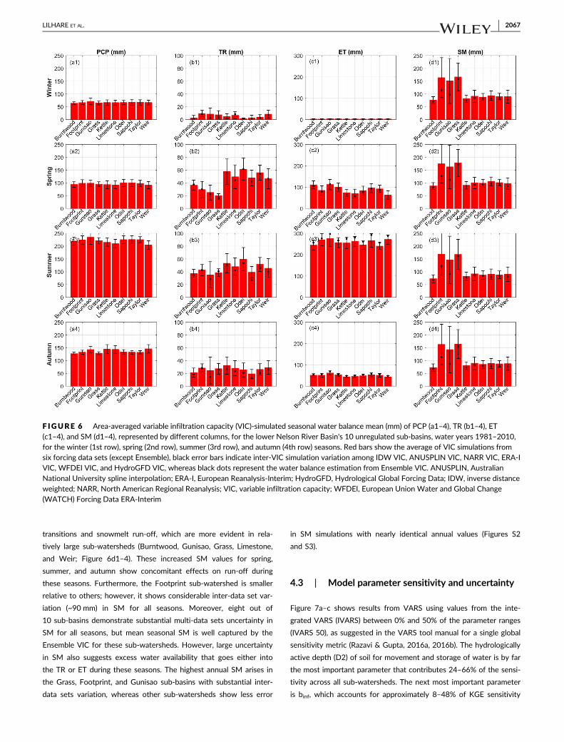
transitions and snowmelt run-off, which are more evident in rela-

tively large sub-watersheds (Burntwood, Gunisao, Grass, Limestone,

and Weir; Figure 6d1–4). These increased SM values for spring,

summer, and autumn show concomitant effects on run-off during

these seasons. Furthermore, the Footprint sub-watershed is smaller

relative to others; however, it shows considerable inter-data set var-

iation (~90 mm) in SM for all seasons. Moreover, eight out of

10 sub-basins demonstrate substantial multi-data sets uncertainty in

SM for all seasons, but mean seasonal SM is well captured by the

Ensemble VIC for these sub-watersheds. However, large uncertainty

in SM also suggests excess water availability that goes either into

the TR or ET during these seasons. The highest annual SM arises in

the Grass, Footprint, and Gunisao sub-basins with substantial inter-

data sets variation, whereas other sub-watersheds show less error

in SM simulations with nearly identical annual values (Figures S2

and S3).

4.3 | Model parameter sensitivity and uncertainty

Figure 7a–c shows results from VARS using values from the inte-

grated VARS (IVARS) between 0% and 50% of the parameter ranges

(IVARS 50), as suggested in the VARS tool manual for a single global

sensitivity metric (Razavi & Gupta, 2016a, 2016b). The hydrologically

active depth (D2) of soil for movement and storage of water is by far

the most important parameter that contributes 24–66% of the sensi-

tivity across all sub-watersheds. The next most important parameter

is binf, which accounts for approximately 8–48% of KGE sensitivity

F IGURE 6 Area-averaged variable infiltration capacity (VIC)-simulated seasonal water balance mean (mm) of PCP (a1–4), TR (b1–4), ET(c1–4), and SM (d1–4), represented by different columns, for the lower Nelson River Basin's 10 unregulated sub-basins, water years 1981–2010,for the winter (1st row), spring (2nd row), summer (3rd row), and autumn (4th row) seasons. Red bars show the average of VIC simulations fromsix forcing data sets (except Ensemble), black error bars indicate inter-VIC simulation variation among IDW VIC, ANUSPLIN VIC, NARR VIC, ERA-IVIC, WFDEI VIC, and HydroGFD VIC, whereas black dots represent the water balance estimation from Ensemble VIC. ANUSPLIN, AustralianNational University spline interpolation; ERA-I, European Reanalysis-Interim; HydroGFD, Hydrological Global Forcing Data; IDW, inverse distanceweighted; NARR, North American Regional Reanalysis; VIC, variable infiltration capacity; WFDEI, European Union Water and Global Change(WATCH) Forcing Data ERA-Interim

LILHARE ET AL. 2067

across all sub-watersheds. Together, these two parameters contribute

to nearly 40–88% of the KGE sensitivity. In the Grass River sub-

watershed, Dsmax, which is the maximum velocity of baseflow for each

grid cell, also becomes important (~30%) in controlling the amount of

run-off generated at the sub-basin outlet. Note that physically inter-

linked parameters (D2 and Dsmax) together have almost the same sen-

sitivity ratio in the Grass River. Ds (fraction of the Dsmax parameter) is

the third most important parameter, and Ws, the fraction of maximum

soil moisture, is also among the more influential parameters in most of

the sub-watersheds. Seasonal sensitivity of model parameters

changes substantially; for example, in winter, Ds and Dsmax, which

control baseflow, become the most sensitive parameters (>25%) over

all sub-basins, whereas in spring and summer, D2 still plays a domi-

nant role in computing sub-surface flow (Figure S4a). Autumn shows

Dsmax as the most sensitive parameter because most of the water

comes from baseflow during this season.

For NSE, the D2 parameter becomes dominant by a large margin

in six out of 10 sub-basins, responsible for 28–70% of the model sen-

sitivity in these sub-watersheds (Figure 7b). This is not the case for

the other four sub-basins (Kettle, Limestone, Odei, and Weir) where

binf remains the most influential factor controlling predictions of low

flows. For the Footprint and Grass, Ws is also influential (~17%). Ws

emerges as the third most important parameter in most of the sub-

basins. Seasonal sensitivity of model parameters changes

substantially; for example, in winter, Ds and Dsmax, which control

baseflow, become the most sensitive parameters over all sub-basins,

whereas in spring and summer, binf and D2 play dominant roles in

establishing streamflow (Figure S4b). The binf parameter shows >45%

ratios of factor sensitivity in spring for most of the sub-watersheds

that reflects excess water availability for infiltration during snowmelt

seasons. Autumn shows Dsmax and D2 as the most sensitive parame-

ters because they are responsible in generating seasonal peak flows.

The total flow volume measured by PBIAS shows D2 as the most

influential parameter that determines maximum water storage in soils

and thus streamflow (Figure 7c). The ratio of sensitivity for this

parameter exceeds 50% for nine sub-basins and nears 80% in three of

them. Unlike the KGE and NSE cases, the baseflow parameters

(Ds and Dsmax) are not important for PBIAS because they have no

effect on the total flow volume. Overall, for PBIAS, binf and D2 are

influential parameters followed by Dsmax. This is due to the influence

of all these parameters in controlling surface and subsurface water

storages. In all sub-basins, the depth of the second soil layer is more

important than the third soil layer. This is perhaps because (a) the third

layer is much thicker than the other two layers and (b) the second

layer has a larger control on infiltration and ET. Seasonal sensitivity of

model parameters for PBIAS is similar to KGE and NSE as the sensi-

tive parameters (i.e., D2, binf, Ds, and Dsmax) are responsible for

streamflow magnitudes and interlinked with each other (Figure S4c).

F IGURE 7 Ratio of factor sensitivity(%) of IVARS 50 for each parameter atannual scale over all sub-watersheds ofthe lower Nelson River Basin for thethree model performance metrics(1981–2010): (a) KGE, (b) NSE, and(c) PBIAS. Ratio of factor sensitivity isestimated by normalizing IVARS50 values in each case, so they add up to

100% for all parameters. IVARS,integrated variogram analysis of responsesurfaces; KGE, Kling–Gupta efficiency;NSE, Nash–Sutcliffe efficiency; PBIAS,percent bias

2068 LILHARE ET AL.

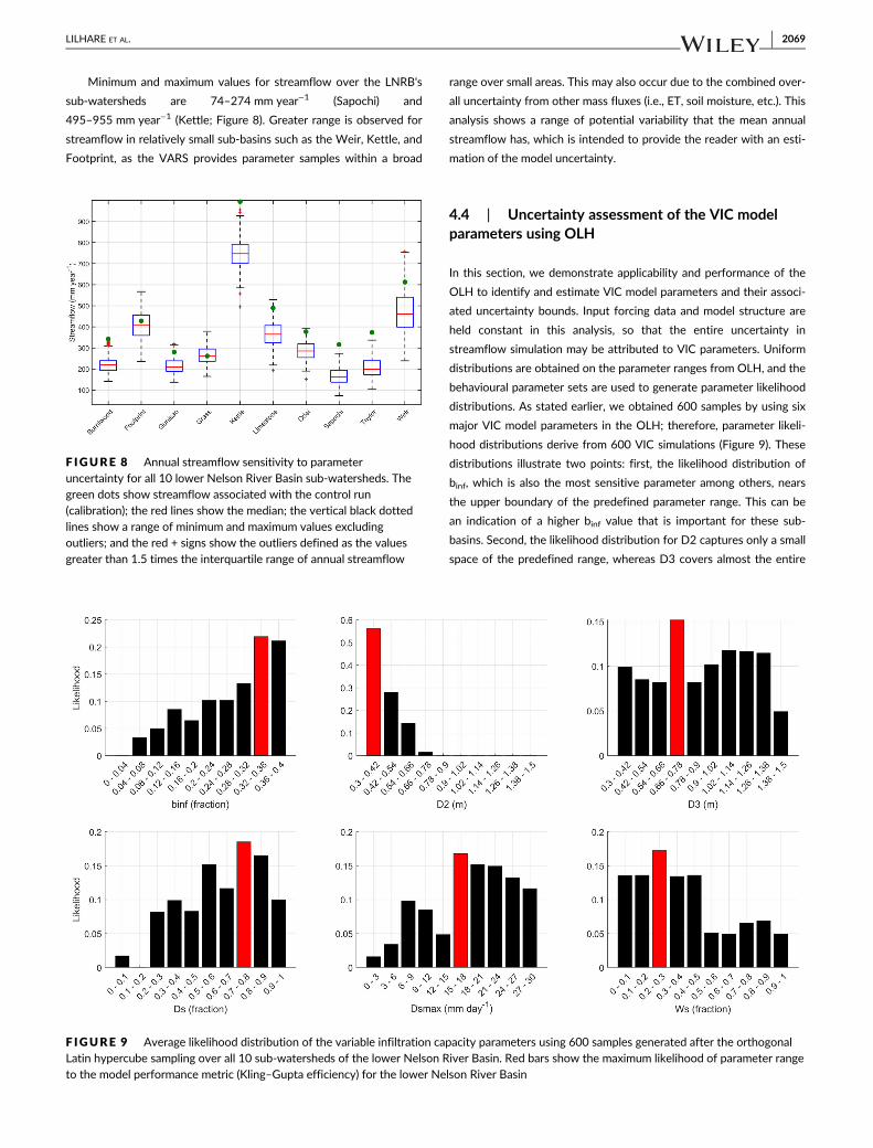
Minimum and maximum values for streamflow over the LNRB's

sub-watersheds are 74–274 mm year−1 (Sapochi) and

495–955 mm year−1 (Kettle; Figure 8). Greater range is observed for

streamflow in relatively small sub-basins such as the Weir, Kettle, and

Footprint, as the VARS provides parameter samples within a broad

range over small areas. This may also occur due to the combined over-

all uncertainty from other mass fluxes (i.e., ET, soil moisture, etc.). This

analysis shows a range of potential variability that the mean annual

streamflow has, which is intended to provide the reader with an esti-

mation of the model uncertainty.

4.4 | Uncertainty assessment of the VIC modelparameters using OLH

In this section, we demonstrate applicability and performance of the

OLH to identify and estimate VIC model parameters and their associ-

ated uncertainty bounds. Input forcing data and model structure are

held constant in this analysis, so that the entire uncertainty in

streamflow simulation may be attributed to VIC parameters. Uniform

distributions are obtained on the parameter ranges from OLH, and the

behavioural parameter sets are used to generate parameter likelihood

distributions. As stated earlier, we obtained 600 samples by using six

major VIC model parameters in the OLH; therefore, parameter likeli-

hood distributions derive from 600 VIC simulations (Figure 9). These

distributions illustrate two points: first, the likelihood distribution of

binf, which is also the most sensitive parameter among others, nears

the upper boundary of the predefined parameter range. This can be

an indication of a higher binf value that is important for these sub-

basins. Second, the likelihood distribution for D2 captures only a small

space of the predefined range, whereas D3 covers almost the entire

F IGURE 8 Annual streamflow sensitivity to parameteruncertainty for all 10 lower Nelson River Basin sub-watersheds. Thegreen dots show streamflow associated with the control run(calibration); the red lines show the median; the vertical black dottedlines show a range of minimum and maximum values excludingoutliers; and the red + signs show the outliers defined as the valuesgreater than 1.5 times the interquartile range of annual streamflow

F IGURE 9 Average likelihood distribution of the variable infiltration capacity parameters using 600 samples generated after the orthogonalLatin hypercube sampling over all 10 sub-watersheds of the lower Nelson River Basin. Red bars show the maximum likelihood of parameter rangeto the model performance metric (Kling–Gupta efficiency) for the lower Nelson River Basin

LILHARE ET AL. 2069

parameter range. However, the hydrograph uncertainty bounds,

which come from the top 10% of OLH runs, associated with these

parameter ranges do not cover the expected number of observed

streamflow values (dark blue region in Figure 10). This can be argued

as a problem of over conditioning the selected relationships between

observed and modelled output (Bermúdez et al., 2017). The Footprint

and Weir sub-watersheds have the widest uncertainty envelopes

whereas the Burntwood, Limestone, Odei, Sapochi, and Taylor sub-

watersheds show relatively narrow uncertainty bounds from the OLH

simulation. This may depend on watershed area, as parameter

F IGURE 10 Streamflow prediction uncertainty associated with estimated parameters from the OLH. Top 10% (shown in blue colour) of OLHsamples, based on Kling–Gupta efficiency, used for the prediction of streamflow for all 10 sub-watersheds, water years 1981–2010. Note that y-axis scales vary between panels. Shaded area (grey colour) shows the envelope of variable infiltration capacity runs from 600 OLH samples. OLH,

orthogonal Latin hypercube

2070 LILHARE ET AL.

variation among a broad range of values over small sub-basins

(e.g., Footprint and Weir) yields greater streamflow uncertainty than

for relatively larger ones (e.g., Burntwood, Limestone, Odei, Sapochi,

and Taylor). Even though the other 90% prediction uncertainty range

(light grey region in Figure 10) captures all observations, it remains

quite wide compared with observations and reveals a notable uncer-

tainty range (0.5–1 mm day−1) in the model parameters, as other con-

ditions are static in this analysis.

5 | DISCUSSION

5.1 | Input data uncertainty

The underestimation in flows from the IDW VIC and ANUSPLIN VIC

simulations reflect the precipitation undercatch and dry bias in these

data sets over the LNRB (Lilhare et al., 2019). As the model resolution

and other configuration (i.e., soil type, land use, etc.) are similar for all

VIC simulations, different values of model performance metrics

exhibit uncertainty associated only with input forcing data sets. These

simulations show substantial disagreement in the run-off with

observed hydrographs, especially in the Kettle, Limestone, Odei,

Sapochi, and Weir sub-basins, owing to the dry bias and undercatch

issues in the precipitation data. Consistent with our previous findings,

the wet (warm) ERA-I and WFDEI precipitation (mean air temperature)

over the LNRB in spring, summer, and autumn induce more surface

run-off and snowmelt that overestimate simulated flows (Figure 4;

Lilhare et al., 2019). Moreover, shifts in the hydrographs may be asso-

ciated with warmer air temperatures over these sub-basins that cause

earlier snowmelt run-off. Such variation in the simulated run-off,

especially during the snowmelt period (April–July), is either due to the

uncertain amount and timing of precipitation or air temperature in

input forcing data sets (Lilhare et al., 2019).

Other sources of uncertainties in water budget estimation may

be the dry (wet) bias in precipitation that results in poor calibration

where model parameters cannot achieve optimal values due to less

(excess) water availability. Consequently, these precipitation uncer-

tainties among all sub-watersheds translate to a minimum (maxi-

mum) 14.0 (88.8) mm year−1 error in the water balance estimates.

These results correspond well with those of Fekete et al. (2010)

who found that the uncertainty in precipitation forcing translates to

at least the same, or typically more substantial, uncertainty in run-

off and related water balance terms. The simulated TR uncertainty

is higher in spring and summer than fall and winter, which is mainly

due to the more substantial seasonal variation in inter-data sets pre-

cipitation and air temperature. However, there remains much uncer-

tainty in air temperature records over the LNRB from the different

forcing data sets. This uncertainty can be translated into inter-

seasonal water balance estimation through run-off and ET pro-

cesses, which are more sensitive to air temperature. The sub-basins

that are more susceptible to ET loss with relatively more surface

water coverage, that is, the Grass and Gunisao, will, therefore, have

higher uncertainty propagation from input data. This represents

both time and space dimensionality to the uncertainty and plays a

critical role in climate change studies where changes in run-off are

most important.

Given that the domain average air temperature and precipitation

differ across VIC forcings, the choice of VIC calibration and validation

periods may induce uncertainty in water balance simulations. There-

fore, calibration using different forcing data over 5–10 years may gen-

erate biases in simulated water balance conditions, as only a wet or

dry period may be captured. Intercomparison of precipitation par-

titioning across various land surface models showed that specific rep-

resentation and parameterizations for water balance components

(i.e., ET and TR) were not consistent across models (Andresen et al.,

2019). However, some models maintained similar run-off and precipi-

tation ratios throughout the simulation; in contrast, VIC showed shifts

from a run-off-dominated system to an ET-dominated system over

permafrost regions in the Northern Hemisphere north of 45�N

(Andresen et al., 2019).

5.2 | Model parameter sensitivity and uncertaintyassessment

The sensitivity of model outputs to selected parameters is justified

given the formulations of the variable infiltration and baseflow gener-

ation curve that form the foundation of the VIC architecture (Liang

et al., 1994, 1996) and as these parameters are traditionally applied in

model calibration (i.e., Elsner et al., 2010). As reported in previous

studies, sensitivity to these parameters hold in both current and

future climate scenarios (Bennett et al., 2018; Christensen &

Lettenmaier, 2007; Demaria et al., 2007). A previous effort used vari-

ous objective functions and found that binf and D2 were the most sen-

sitive parameters followed by the drainage parameter among 10 VIC

parameters across four American river basins of different hydro-

climates (Demaria et al., 2007). Xie and Yuan (2006) manually varied

four VIC parameters from ±10% to ±25% to perform SA over

12 watersheds in France, finding baseflow and soil depth related

parameters as the most sensitive one. These studies either used man-

ual analysis methods or limited objective functions at annual timescale

to examine the parameter sensitivity. In contrast, we apply a more

robust, automated, and efficient approach at seasonal and annual

timescales to determine the parameter sensitivity and its seasonal

importance over 10 subarctic watersheds. Moreover, the SA method

takes multiple objective functions into account that provide more

robust estimates of parameter sensitivity.

The high values of IVARS 50 for D2 are caused partly by the

interaction of this parameter with other model parameters (e.g., soil

profile and root depth) and its relatively large range of values. The Ds

and Dsmax parameters influence baseflow, which have a higher impact

on low-flow predictions. Therefore, these parameters become impor-

tant for NSE in some sub-basins (Grass and Footprint) as they control

the timing of low flows. Moreover, in PBIAS, high values of D2 indi-

cate its considerable interaction on model responses as D2 character-

izes the seasonal soil moisture behaviour but by no means binf as

LILHARE ET AL. 2071

being perhaps also an important parameter over the LNRB. Overall,

for PBIAS, binf and D2 are influential parameters followed by Dsmax.

This is due to the influence of all these parameters in controlling sur-

face and subsurface water storages. In all sub-basins, D2 is more

important than D3. This is perhaps because of (a) the third layer is

much thicker than the other two layers and (b) the second layer has a

larger control on infiltration and ET.

There is general agreement between the NSE and KGE sensitiv-

ity experiments over most sub-watersheds, particularly in identifying

the most influential parameters. Nonetheless, parameter sensitivity

depends on metric choice and varies significantly according to

model performance metrics. For example, the D2 parameter is quite

important for KGE and PBIAS in most of the rivers but has slightly

less impact on NSE. This is because D2 controls baseflow and thus

the timing of flows, which is important particularly for peak flows

represented by NSE. However, flow timing is not important when

assessing total flow volume represented by PBIAS. Similarly, binf is

less important for KGE and PBIAS but more influential for NSE over

most sub-basins through its control of available infiltration capacity,

thereby influencing peak flows and soil water volumes. Moreover,

seasonality and wet or dry years may yield different SA results,

which should be noted as a cautionary tale for using SA as a

precalibration methodology. Consequently, to better understand the

dominant controls on model behaviour, multiple criteria should be

considered.

These results reinforce the well-known conclusion that for most

effective SA results, one should select SA criteria in alignment with

the final goals of the modelling application (e.g., flood forecasting,

drought analysis, or water balance assessment). Regardless of the

metric choice, often a limited number of parameters control most of

the model response variations. This has important implications such as

minimizing the dimensionality of the optimization process

(i.e., calibration) through emphasis on a few influential parameters to

generate reliable results. Even if fixed values for these influential

parameters cannot be prescribed, any available information including

observational data may reduce parameter ranges during calibration.

This is generally true for all parameters and greatly increases the

identifiability of our modelling application, which is often overlooked.

Moreover, this also fits with the International Association of Hydro-

logical Sciences' (IAHS) 23 unsolved problems in hydrology initiatives

focused on understanding process changes, which control changing

run-off response (Blöschl et al., 2019). Moreover, using these SA

results, one can focus on specific model parameters and their value

ranges, thus diminishing computational burdens, by fixing the value of

non-essential parameters.

6 | CONCLUSION

This exercise provides valuable new insights into the internal func-

tioning of models and allows the provision of impactful recommen-

dations for improving development and application of the VIC

model. In this respect, we found that daily precipitation is more

important than air temperature for annual and seasonal water bal-

ance estimates. The choice of model performance metric signifi-

cantly affects the sensitivity assessment. Therefore, to obtain in-

depth understanding of model behaviour, SA using multiple criteria

should be adopted, which capture distinct characteristics of the

model response.

SA results can be used more effectively when aligned with the

final goals of the model application (e.g., flood forecasting and drought

monitoring). SA results depend on various factors such as hydro-

climatic conditions, model configuration, input forcing, land cover clas-

ses, initial state, vegetation parameters, and so forth, and these can

have a large impact on model behaviour. We considered a full range

of parameters that can influence their ratio of factor sensitivity if the

range changes in other applications. SA can identify aspects of the

model internal functioning that are counterintuitive and thus assist

modellers to diagnose possible model deficiencies and make recom-

mendations for end users. The calibration process identified a set of

influential parameters that assists VIC users in reducing prediction

uncertainty by providing a more robust, accurate, and less computa-

tionally intensive calibration effort. Overall, parameters for the second

soil layer depth and variable infiltration curve dominate the control of

streamflow prediction in VIC followed by the Ds and Dsmax parame-

ters. The VIC community may prioritize these parameters during

model calibration for similar physical and climatic environments.

Although this study focused on VARS sensitivity and OLH uncertainty

analysis, a multicriteria SA approach under various conditions may

lead to improved understanding of model structure, reductions in pre-

diction uncertainty, and more efficient parameter calibration. Potential

future work could investigate the effects of initial or boundary condi-

tions and/or other model variables such as soil moisture or ET in

model sensitivity assessments.

AUTHOR CONTRIBUTIONS

All authors designed the study. R. L. and S. P. developed the VARS-

coupled VIC MATLAB codes and methodology. R. L. extracted hydro-

metric data, performed VIC and VARS simulations, computed the

hydrographs, performed the sensitivity and uncertainty analyses, and

drafted figures with support from S. P., S. J. D., and T. A. S. R. L. wrote

the manuscript with contributions from all co-authors, and all contrib-

uted to manuscript refinement and revisions.

ACKNOWLEDGMENTS

Financial and in-kind support for this research was provided by Mani-

toba Hydro, ArcticNet, and the Natural Sciences and Engineering

Research Council of Canada (NSERC) through the BaySys project.

Mark Gervais, Philip Slota, Mike Vieira, and Shane Wruth (Manitoba

Hydro) provided helpful advice and logistical support throughout this

work and beneficial reviews on an earlier version of the manuscript.

Thanks to UNBC's NHG members Siraj Ul Islam and Aseem Raj

Sharma for providing access to and information on gridded climate

data sets. Thanks to two anonymous reviewers and the handling edi-

tor for their constructive and insightful comments that led to a much

improved paper.

2072 LILHARE ET AL.

DATA AVAILABILITY STATEMENT

The forcing data that support the findings of this study are openly

available online: for IDW at http://climate.weather.gc.ca/his-

torical_data/search_historic_data_e.html, ANUSPLIN at https://cfs.

nrcan.gc.ca/projects/3, NARR at https://www.esrl.noaa.gov/psd/

data/gridded/data.narr.html, ERA-I at https://apps.ecmwf.int/

datasets/data/interim-full-daily/levtype=sfc/, WFDEI at https://rda.

ucar.edu/datasets/ds314.2/#!description, and HydroGFD at https://

hypeweb.smhi.se. The hydrometric data from Water Survey of

Canada are publicly available at https://wateroffice.ec.gc.ca. The VIC

simulations are available upon request from the authors.

ORCID

Rajtantra Lilhare https://orcid.org/0000-0002-6913-6024

Scott Pokorny https://orcid.org/0000-0001-6665-5622

Stephen J. Déry https://orcid.org/0000-0002-3553-8949

Tricia A. Stadnyk https://orcid.org/0000-0002-2145-4963

Kristina A. Koenig https://orcid.org/0000-0002-1570-3820

REFERENCES

Abebe, N. A., Ogden, F. L., & Pradhan, N. R. (2010). Sensitivity and uncer-

tainty analysis of the conceptual HBV rainfall–runoff model: Implica-

tions for parameter estimation. Journal of Hydrology, 389(3–4),301–310.

Anderson, J., Chung, F., Anderson, M., Brekke, L., Easton, D., Ejeta, M., …Snyder, R. (2008). Progress on incorporating climate change into man-

agement of California's water resources. Climatic Change, 87, 91–108.Andresen, C. G., Lawrence, D. M., Wilson, C. J., McGuire, A. D., Koven, C.,

Schaefer, K., … Zhang, W. (2019). Soil moisture and hydrology projec-

tions of the permafrost region: A model intercomparison. The

Cryosphere Discussions, 1–20. https://doi.org/10.5194/tc-2019-144Aster, R. C., Borchers, B., & Thurber, C. H. (2013). Parameter estimation

and inverse problems (2nd ed.). Retrieved from https://www.elsevier.

com/books/parameter-estimation-and-inverse-problems/aster/978-0-

12-385048-5

Bennett, K. E., Blanco, J. R. U., Jonko, A., Bohn, T. J., Atchley, A. L.,

Urban, N. M., & Middleton, R. S. (2018). Global sensitivity of simulated

water balance indicators under future climate change in the Colorado

Basin. Water Resources Research, 54(1), 132–149. https://doi.org/10.1002/2017WR020471

Berg, P., Donnelly, C., & Gustafsson, D. (2018). Near-real-time adjusted

reanalysis forcing data for hydrology. Hydrology and Earth System Sci-

ences, 22(2), 989–1000. https://doi.org/10.5194/hess-22-989-2018Bermúdez, M., Neal, J. C., Bates, P. D., Coxon, G., Freer, J. E., Cea, L., &

Puertas, J. (2017). Quantifying local rainfall dynamics and uncertain

boundary conditions into a nested regional-local flood modeling sys-

tem. Water Resources Research, 53(4), 2770–2785. https://doi.org/10.1002/2016WR019903

Beven, K., & Binley, A. (1992). The future of distributed models: Model cal-

ibration and uncertainty prediction. Hydrological Processes, 6(3),

279–298. https://doi.org/10.1002/hyp.3360060305Blöschl, G., Bierkens, M. F. P., Chambel, A., Cudennec, C., Destouni, G.,

Fiori, A., … Zhang, Y. (2019). Twenty-three unsolved problems in

hydrology (UPH) – A community perspective. Hydrological Sciences

Journal, 64(10), 1141–1158. https://doi.org/10.1080/02626667.

2019.1620507

Boucher, O., & Best, M. (2010). The WATCH forcing data 1958-2001: A

meteorological forcing dataset for land surface- and hydrological-

models. In WATCH technical report. Wallingford Oxfordshire, UK:

Water and Global Change.

Bowling, L. C., & Lettenmaier, D. P. (2010). Modeling the effects of lakes

and wetlands on the water balance of arctic environments. Journal of

Hydrometeorology, 11(2), 276–295. https://doi.org/10.1175/2009

JHM1084.1

Bowling, L. C., Lettenmaier, D. P., Nijssen, B., Graham, L. P., Clark, D. B., El

Maayar, M., … Yang, Z. (2003). Simulation of high-latitude hydrological

processes in the Torne–Kalix basin: PILPS phase 2 (e): 1: Experiment

description and summary intercomparisons. Global and Planetary

Change, 38(1), 1–30.Cherkauer, K. A., & Lettenmaier, D. P. (1999). Hydrologic effects of frozen

soils in the upper Mississippi River basin. Journal of Geophysical

Research: Atmospheres, 104(D16), 19599–19610.Cherkauer, K. A., & Lettenmaier, D. P. (2003). Simulation of spatial variabil-

ity in snow and frozen soil. Journal of Geophysical Research: Atmo-

spheres, 108(D22), 8858. https://doi.org/10.1029/2003JD003575

Christensen, N. S., & Lettenmaier, D. P. (2007). A multimodel ensemble

approach to assessment of climate change impacts on the hydrology

and water resources of the Colorado River basin. Hydrology and Earth

System Sciences, 11(4), 1417–1434. https://doi.org/10.5194/hess-11-1417-2007

Cosby, B. J., Hornberger, G. M., Clapp, R. B., & Ginn, T. (1984). A statistical

exploration of the relationships of soil moisture characteristics to the

physical properties of soils. Water Resources Research, 20(6), 682–690.Dee, D. P., Uppala, S. M., Simmons, A. J., Berrisford, P., Poli, P.,

Kobayashi, S., … Vitart, F. (2011). The ERA-interim reanalysis: Configu-

ration and performance of the data assimilation system. Quarterly Jour-

nal of the Royal Meteorological Society, 137(656), 553–597. https://doi.org/10.1002/qj.828

Demaria, E. M., Nijssen, B., & Wagener, T. (2007). Monte Carlo sensitivity

analysis of land surface parameters using the variable infiltration

capacity model. Journal of Geophysical Research: Atmospheres, 112,

D11113. https://doi.org/10.1029/2006JD007534

Döll, P., Kaspar, F., & Lehner, B. (2003). A global hydrological model for

deriving water availability indicators: Model tuning and validation.

Journal of Hydrology, 270(1), 105–134.Duan, Q., Sorooshian, S., & Gupta, V. (1992). Effective and efficient global

optimization for conceptual rainfall-runoff models. Water Resources

Research, 28(4), 1015–1031. https://doi.org/10.1029/91WR02985

Elsner, M. M., Cuo, L., Voisin, N., Deems, J. S., Hamlet, A. F., Vano, J. A., …Lettenmaier, D. P. (2010). Implications of 21st century climate change

for the hydrology of Washington State. Climatic Change, 102(1–2),225–260.

Eum, H.-I., Dibike, Y., Prowse, T., & Bonsal, B. (2014). Inter-comparison of

high-resolution gridded climate data sets and their implication on

hydrological model simulation over the Athabasca Watershed, Canada.

Hydrological Processes, 28(14), 4250–4271.Fekete, B. M., Vörösmarty, C. J., Roads, J. O., & Willmott, C. J. (2004).

Uncertainties in precipitation and their impacts on runoff estimates.

Journal of Climate, 17(2), 294–304.Fekete, B. M., Wisser, D., Kroeze, C., Mayorga, E., Bouwman, L.,

Wollheim, W. M., & Vörösmarty, C. (2010). Millennium ecosystem

assessment scenario drivers (1970–2050): Climate and hydrological

alterations. Global Biogeochemical Cycles, 24(4). Washington, D.C.:

American Geophysical Union. https://doi.org/10.1029/2009GB00

3593

Fowler, H. J., Ekström, M., Blenkinsop, S., & Smith, A. P. (2007). Estimating

change in extreme European precipitation using a multimodel ensem-

ble. Journal of Geophysical Research: Atmospheres, 112, D18104.

https://doi.org/10.1029/2007JD008619

Fowler, H. J., & Kilsby, C. G. (2007). Using regional climate model data to

simulate historical and future river flows in Northwest England. Cli-

matic Change, 80(3–4), 337–367.Frey, H. C., & Patil, S. R. (2002). Identification and review of sensitivity

analysis methods. Risk Analysis, 22(3), 553–578. https://doi.org/10.1111/0272-4332.00039

LILHARE ET AL. 2073

Gan, Y., Duan, Q., Gong, W., Tong, C., Sun, Y., Chu, W., … Di, Z. (2014). A

comprehensive evaluation of various sensitivity analysis methods: A

case study with a hydrological model. Environmental Modelling & Soft-

ware, 51, 269–285. https://doi.org/10.1016/j.envsoft.2013.09.031Gemmer, M., Becker, S., & Jiang, T. (2004). Observed monthly precipitation

trends in China 1951–2002. Theoretical and Applied Climatology, 77

(1–2), 39–45. https://doi.org/10.1007/s00704-003-0018-3Gerten, D., Schaphoff, S., Haberlandt, U., Lucht, W., & Sitch, S. (2004). Ter-

restrial vegetation and water balance—Hydrological evaluation of a

dynamic global vegetation model. Journal of Hydrology, 286(1), 249–270.Goldberg, D. E. (1989). Genetic algorithms in search, optimization, and

machine learning. Reading, MA: Addison Wesley Publishing Company.

Gupta, H. V., Kling, H., Yilmaz, K. K., & Martinez, G. F. (2009). Decomposi-

tion of the mean squared error and NSE performance criteria: Implica-

tions for improving hydrological modelling. Journal of Hydrology, 377

(1–2), 80–91. https://doi.org/10.1016/j.jhydrol.2009.08.003Hill, M. C., & Tiedeman, C. R. (2007). Effective groundwater model calibra-

tion: With analysis of data, sensitivities, predictions, and uncertainty.

Hoboken, NJ: John Wiley & Sons.

Hopkinson, R. F., McKenney, D. W., Milewska, E. J., Hutchinson, M. F.,

Papadopol, P., & Vincent, L. A. (2011). Impact of aligning climatological

day on gridding daily maximum–minimum temperature and precipita-

tion over Canada. Journal of Applied Meteorology and Climatology, 50

(8), 1654–1665.Hostetler, S. W. (1991). Simulation of lake ice and its effect on the late-

Pleistocene evaporation rate of Lake Lahontan. Climate Dynamics, 6(1),

43–48. https://doi.org/10.1007/BF00210581Hostetler, S. W., & Bartlein, P. J. (1990). Simulation of lake evaporation

with application to modeling lake level variations of Harney-Malheur

Lake, Oregon. Water Resources Research, 26(10), 2603–2612. https://doi.org/10.1029/WR026i010p02603

Hundecha, Y., St-Hilaire, A., Ouarda, T., El Adlouni, S., & Gachon, P. (2008).

A nonstationary extreme value analysis for the assessment of changes

in extreme annual wind speed over the Gulf of St. Lawrence, Canada.

Journal of Applied Meteorology and Climatology, 47(11), 2745–2759.Iman, R. L., & Helton, J. C. (1988). An investigation of uncertainty and sen-

sitivity analysis techniques for computer models. Risk Analysis, 8(1),

71–90. https://doi.org/10.1111/j.1539-6924.1988.tb01155.xIslam, S. U., & Déry, S. J. (2017). Evaluating uncertainties in modelling the

snow hydrology of the Fraser River basin, British Columbia, Canada.

Hydrology and Earth System Sciences, 21(3), 1827–1847. https://doi.org/10.5194/hess-21-1827-2017

Kang, D. H., Gao, H., Shi, X., Islam, S. u., & Déry, S. J. (2016). Impacts of a

rapidly declining mountain snowpack on streamflow timing in

Canada's Fraser River basin. Scientific Reports, 6, 19299. https://doi.

org/10.1038/srep19299

Kavetski, D., Kuczera, G., & Franks, S. W. (2006). Calibration of conceptual

hydrological models revisited: 2. Improving optimisation and analysis.

Journal of Hydrology, 320(1), 187–201. https://doi.org/10.1016/j.

jhydrol.2005.07.013

Li, L., & Xu, C.-Y. (2014). The comparison of sensitivity analysis of hydrological

uncertainty estimates by GLUE and Bayesian method under the impact

of precipitation errors. Stochastic Environmental Research and Risk Assess-

ment, 28(3), 491–504. https://doi.org/10.1007/s00477-013-0767-1Liang, X., & Guo, J. (2003). Intercomparison of land-surface parameteriza-

tion schemes: Sensitivity of surface energy and water fluxes to model

parameters. Journal of Hydrology, 279(1), 182–209. https://doi.org/10.1016/S0022-1694(03)00168-9

Liang, X., Lettenmaier, D. P., Wood, E. F., & Burges, S. J. (1994). A simple

hydrologically based model of land surface water and energy fluxes for

general circulation models. Journal of Geophysical Research: Atmo-

spheres, 99(D7), 14415–14428.Liang, X., Wood, E. F., & Lettenmaier, D. P. (1996). Surface soil moisture

parameterization of the VIC-2L model: Evaluation and modification.

Global and Planetary Change, 13(1), 195–206.

Liang, X., Wood, E. F., & Lettenmaier, D. P. (1999). Modeling ground heat

flux in land surface parameterization schemes. Journal of Geophysical

Research: Atmospheres, 104(D8), 9581–9600. https://doi.org/10.

1029/98JD02307

Liang, X., Xie, Z., & Huang, M. (2003). A new parameterization for surface

and groundwater interactions and its impact on water budgets with

the variable infiltration capacity (VIC) land surface model. Journal of

Geophysical Research: Atmospheres, 108(D16), 8613. https://doi.org/

10.1029/2002JD003090

Lilhare, R., Déry, S. J., Pokorny, S., Stadnyk, T. A., & Koenig, K. A. (2019).

Inter-comparison of multiple hydro-climatic datasets across the lower

Nelson River basin, Manitoba, Canada. Atmosphere-Ocean, 57(4),

262–278. https://doi.org/10.1080/07055900.2019.1638226Liu, Y., & Gupta, H. V. (2007). Uncertainty in hydrologic modeling: Toward

an integrated data assimilation framework. Water Resources Research,

43, W07401. https://doi.org/10.1029/2006WR005756

Mao, D., & Cherkauer, K. A. (2009). Impacts of land-use change on hydro-

logic responses in the Great Lakes region. Journal of Hydrology, 374(1),

71–82.Maurer, E. P., Wood, A. W., Adam, J. C., Lettenmaier, D. P., & Nijssen, B.

(2002). A long-term hydrologically based dataset of land surface fluxes

and states for the conterminous United States. Journal of Climate, 15

(22), 3237–3251.Mesinger, F., DiMego, G., Kalnay, E., Mitchell, K., Shafran, P. C.,

Ebisuzaki, W., … Shi, W. (2006). North American regional reanalysis.

Bulletin of the American Meteorological Society, 87(3), 343–360.https://doi.org/10.1175/BAMS-87-3-343

Miller, D. A., & White, R. A. (1998). A conterminous United States multi-

layer soil characteristics dataset for regional climate and hydrology

modeling. Earth Interactions, 2(2), 1–26.Mishra, V., & Lilhare, R. (2016). Hydrologic sensitivity of Indian sub-

continental river basins to climate change. Global and Planetary

Change, 139, 78–96. https://doi.org/10.1016/j.gloplacha.2016.01.003Myneni, R. B., Ramakrishna, R., Nemani, R., & Running, S. W. (1997). Esti-

mation of global leaf area index and absorbed PAR using radiative

transfer models. IEEE Transactions on Geoscience and Remote Sensing,

35(6), 1380–1393.Nash, J., & Sutcliffe, J. V. (1970). River flow forecasting through conceptual

models part I—A discussion of principles. Journal of Hydrology, 10(3),

282–290.Natural Resources Canada. (2010, December 31). Permafrost. Retrieved

December 23, 2016, from http://geogratis.gc.ca/api/en/nrcan-rncan/

ess-sst/dc7107c0-8893-11e0-aa10-6cf049291510.html

Natural Resources Canada. (2014). Regional, national and international cli-

mate modeling | Forests | Natural Resources Canada: Introduction.

Retrieved November 3, 2016, from http://cfs.nrcan.gc.ca/projects/3?

lang=en_CA

Natural Resources Canada. (2016). Potential Evapotranspiration—Open

Government Portal. Retrieved April 9, 2018, from https://open.

canada.ca/data/en/dataset/a650fb95-1104-504b-a344-

0fe05877b7cf

Nijssen, B., Lettenmaier, D. P., Liang, X., Wetzel, S. W., & Wood, E. F.

(1997). Streamflow simulation for continental-scale river basins. Water

Resources Research, 33(4), 711–724. https://doi.org/10.1029/96W

R03517

Nijssen, B., Schnur, R., & Lettenmaier, D. P. (2001). Global retrospective

estimation of soil moisture using the variable infiltration capacity land

surface model, 1980-93. Journal of Climate, 14(8), 1790–1808.North American Land Change Monitoring System. (2010). 2010 North

American Land Cover at 250 m spatial resolution. Produced by Natural

Resources Canada/Canadian Center for Remote Sensing (NRCan/

CCRS), United States Geological Survey (USGS); Insituto Nacional de

Estadística y Geografía (INEGI), Comisión Nacional para el Con-

ocimiento y Uso de la Biodiversidad (CONABIO) and Comisión

Nacional Forestal (CONAFOR). Retrieved April 14, 2017, from The

2074 LILHARE ET AL.

USGS Land Cover Institute (LCI) website: http://www.cec.org/tools-

and-resources/map-files/land-cover-2010

Patterson, J. C., & Hamblin, P. F. (1988). Thermal simulation of a lake with

winter ice cover. Limnology and Oceanography, 33(3), 323–338.https://doi.org/10.4319/lo.1988.33.3.0323

Pavelsky, T. M., & Smith, L. C. (2006). Intercomparison of four global pre-

cipitation data sets and their correlation with increased

Eurasian river discharge to the Arctic Ocean. Journal of Geophysical

Research: Atmospheres, 111, D21112. https://doi.org/10.1029/

2006JD007230

Razavi, S., & Gupta, H. V. (2016a). A new framework for comprehensive,

robust, and efficient global sensitivity analysis: 1. Theory. Water

Resources Research, 52(1), 423–439. https://doi.org/10.1002/

2015WR017558

Razavi, S., & Gupta, H. V. (2016b). A new framework for comprehensive,

robust, and efficient global sensitivity analysis: 2. Application. Water

Resources Research, 52(1), 440–455. https://doi.org/10.1002/2015

WR017559

Razavi, S., Sheikholeslami, R., Gupta, H. V., & Haghnegahdar, A. (2019).

VARS-TOOL: A toolbox for comprehensive, efficient, and robust sensi-

tivity and uncertainty analysis. Environmental Modelling & Software,

112, 95–107. https://doi.org/10.1016/j.envsoft.2018.10.005Reed, S., Koren, V., Smith, M., Zhang, Z., Moreda, F., Seo, D.-J., & DMIP

Participants (2004). Overall distributed model intercomparison project

results. Journal of Hydrology, 298(1), 27–60.Sabarly, F., Essou, G., Lucas-Picher, P., Poulin, A., & Brissette, F. (2016).

Use of four reanalysis datasets to assess the terrestrial branch of the

water cycle over Quebec, Canada. Journal of Hydrometeorology, 17(5),

1447–1466.Sauchyn, D., Vanstone, J., & Perez-Valdivia, C. (2011). Modes and forcing

of hydroclimatic variability in the upper North Saskatchewan River

basin since 1063. Canadian Water Resources Journal, 36(3), 205–217.https://doi.org/10.4296/cwrj3603889

Seager, R., Neelin, D., Simpson, I., Liu, H., Henderson, N., Shaw, T., …Cook, B. (2014). Dynamical and thermodynamical causes of large-scale

changes in the hydrological cycle over North America in response to

global warming. Journal of Climate, 27(20), 7921–7948.Shafii, M., Tolson, B., & Matott, L. S. (2015). Addressing subjective

decision-making inherent in GLUE-based multi-criteria rainfall–runoffmodel calibration. Journal of Hydrology, 523, 693–705. https://doi.org/10.1016/j.jhydrol.2015.01.051

Sheffield, J., & Wood, E. F. (2007). Characteristics of global and regional

drought, 1950–2000: Analysis of soil moisture data from off-line simu-

lation of the terrestrial hydrologic cycle. Journal of Geophysical

Research: Atmospheres, 112, D17115. https://doi.org/10.1029/2006

JD008288

Shepard, D. (1968). A two-dimensional interpolation function for

irregularly-spaced data. Proceedings of the 1968 ACM National Confer-

ence (pp. 517–524). New York. http://dx.doi.org/10.1145/800186.

810616

Shi, X., Wood, A. W., & Lettenmaier, D. P. (2008). How essential is hydro-

logic model calibration to seasonal streamflow forecasting? Journal of

Hydrometeorology, 9(6), 1350–1363. https://doi.org/10.1175/2008

JHM1001.1

Stedinger, J. R., Vogel, R. M., Lee, S. U., & Batchelder, R. (2008). Appraisal

of the generalized likelihood uncertainty estimation (GLUE) method.

Water Resources Research, 44(12), W00B06. https://doi.org/10.1029/

2008WR006822

Tapiador, F. J., Turk, F. J., Petersen, W., Hou, A. Y., García-Ortega, E.,

Machado, L. A., … Huffman, G. J. (2012). Global precipitation measure-

ment: Methods, datasets and applications. Atmospheric Research, 104,

70–97.Tobin, C., Nicotina, L., Parlange, M. B., Berne, A., & Rinaldo, A. (2011).

Improved interpolation of meteorological forcings for hydrologic

applications in a Swiss alpine region. Journal of Hydrology, 401(1),

77–89.United States Geological Survey. (2013). Shuttle Radar Topography Mis-

sion (SRTM) 1 Arc-Second Global | The Long Term Archive. Retrieved

April 6, 2017, from https://lta.cr.usgs.gov/SRTM1Arc

USACE. (1956). “Snow hydrology” summary report of the snow investigations.

Portland, Oregon: North Pacific Division, US Army Corps of Engineers.

Van Griensven, A., Meixner, T., Grunwald, S., Bishop, T., Diluzio, M., &

Srinivasan, R. (2006). A global sensitivity analysis tool for the parame-

ters of multi-variable catchment models. Journal of Hydrology, 324

(1–4), 10–23. https://doi.org/10.1016/j.jhydrol.2005.09.008Vrugt, J. A., Diks, C. G., Gupta, H. V., Bouten, W., & Verstraten, J. M.

(2005). Improved treatment of uncertainty in hydrologic modeling:

Combining the strengths of global optimization and data assimilation.

Water Resources Research, 41(1), W01017. https://doi.org/10.1029/

2004WR003059

Vrugt, J. A., Gupta, H. V., Bouten, W., & Sorooshian, S. (2003). A shuffled

complex evolution Metropolis algorithm for optimization and uncer-

tainty assessment of hydrologic model parameters. Water Resources

Research, 39(8), 1201. https://doi.org/10.1029/2002WR001642

Wagener, T., & Gupta, H. V. (2005). Model identification for hydrological

forecasting under uncertainty. Stochastic Environmental Research and

Risk Assessment, 19(6), 378–387.Wang, A., Bohn, T. J., Mahanama, S. P., Koster, R. D., & Lettenmaier, D. P.

(2009). Multimodel ensemble reconstruction of drought over the con-

tinental United States. Journal of Climate, 22(10), 2694–2712.Water Survey of Canada. (2016). Home—Water Office—Environment

Canada. Retrieved January 4, 2017, from http://wateroffice.ec.gc.ca/

Weedon, G. P., Balsamo, G., Bellouin, N., Gomes, S., Best, M. J., &

Viterbo, P. (2014). The WFDEI meteorological forcing data set:

WATCH forcing data methodology applied to ERA-interim reanalysis

data. Water Resources Research, 50(9), 7505–7514.Williams, G. P., & Gold, L. W. (1976). Ground temperatures. CBD-180.

Institute for Research in Construction. Originally Published, (July).

https://doi.org/10.4224/40000712

Woo, M.-K., & Thorne, R. (2006). Snowmelt contribution to discharge from

a large mountainous catchment in subarctic Canada. Hydrological Pro-

cesses, 20(10), 2129–2139.Xie, Z., & Yuan, F. (2006). A parameter estimation scheme of the land surface

model VIC using the MOPEX databases. IAHS Publication, 307, 169–179.Yapo, P. O., Gupta, H. V., & Sorooshian, S. (1998). Multi-objective global

optimization for hydrologic models. Journal of Hydrology, 204(1–4),83–97. https://doi.org/10.1016/S0022-1694(97)00107-8

Zhang, J. L., Li, Y. P., Huang, G. H., Wang, C. X., & Cheng, G. H. (2016).

Evaluation of uncertainties in input data and parameters of a hydrolog-

ical model using a Bayesian framework: A case study of a snowmelt–precipitation-driven watershed. Journal of Hydrometeorology, 17(8),

2333–2350. https://doi.org/10.1175/JHM-D-15-0236.1

SUPPORTING INFORMATION

Additional supporting information may be found online in the

Supporting Information section at the end of this article.

How to cite this article: Lilhare R, Pokorny S, Déry SJ,

Stadnyk TA, Koenig KA. Sensitivity analysis and uncertainty

assessment in water budgets simulated by the variable

infiltration capacity model for Canadian subarctic watersheds.

Hydrological Processes. 2020;34:2057–2075. https://doi.org/

10.1002/hyp.13711

LILHARE ET AL. 2075