uncertainty and sensitivity in global carbon cycle modelling · uncertainty and sensitivity in...

P P

Vol. 9: 157-174, 1998 CLIMATE RESEARCH

Published February 27 Clim Res

Uncertainty and sensitivity in global carbon cycle modelling

Stuart Parkinson*, Peter Young**

Centre for Research into Environmental Systems and Statistics (CRES), Lancaster University, Lancaster, United Kingdom

ABSTRACT This paper summarises the results obtalned from a stochastic sensitivity study in the area of global carbon cycle modelling In parhcular it outlines how Monte Carlo Slrnulation (MCS) techniques and associated Generalised Sensitivity Analysis (GSA) have been applied to a modified box- diffusion model Using pararnetnc and input uncertainty measures denved from independent sources, the analysis shows that the model produces an ensemble response for atmosphenc CO2 whose mean evolution is reasonably consistent with that observed over the industrial penod (1765 to 1990) How- ever, the situation is more ambiguous in relation to the amplitude distribution of the stochastic realisations here, there is a larger than expected vanance ansing from the assumed uncertainty, although this may be due to unavoidable lunitations in the assumptions about parametenc uncertainty used in the MCS analysis The analysis also shows that the a pnon model response is less consistent with I3C measurements and not at all consistent with the I4C observations, while GSA suggests that, from over 20 model parameters, only a small number have a statistically significant effect on the model response in 1990 In addition, the results from MCS, using the IPCC (Intergovernmental Panel on Climate Change) Scenano IS92a inputs, demonstrate that the uncerta~nties in the projections of the CO2 concentrations using this model are significantly higher than those suggested so far using deterministic methods Finally, the advantages and disadvantages of the stochastic methodology are discussed

KEY WORDS: Stochastlc modelling . Uncertainty analysis . Sensitivity analysis . Monte Carlo Simula- tion . Global carbon cycle model . Future carbon dioxide concentrations

1. INTRODUCTION

In the past few years, there has been widespread concern over the possibility of climate change arising from the observed increase in the atmospheric concentrations of the greenhouse gases, particularly carbon dioxide. This has stimulated a growing body of research on the global carbon cycle; and many computer-based mathematical models have been con- structed in an attempt to explain the dynamics of global carbon balance and, in particular, to assess the effects of projected fossil fuel usage and land-use changes into the next millennium. Paradoxically, while the inherent uncertainty in such analysis is often acknowledged, most of these models have been com-

'Present address: Centre for Environmental Strategy, Uni- versity of Surrey, Guildford GU2 5XH, United k n g d o m

"E-mall: [email protected]

pletely deterministic in nature, usually with a fairly large and complex nonlinear structure characterised by a relatively large number of unknown parameters.

Conventionally, a deterministic, physically-based mathematical model of t h s type is based on the currently accepted theoretical paradigms in the field of clunate science; and the parameters in the model, which normally have a perceived physical interpretation, are either estimated directly from laboratory or point source data; obtained by optimisation, so that the model matches the observed time series data to some acceptable degree; or determined by a combination of these methods. In this context, model optirnisation may be formal (e.g. Enting & Lassey 1993) or based on some less objective 'calibration' procedure which involves 'tuning' the parameters within physically justifiable bounds until a reasonable match to the observed data is obtained.

Clearly, the less formal approaches leave much to subjective judgement and are difficult to fully justify in

O Inter-Research 1998

158 Clim Res 9:

statistical terms; while the formal optimisation methods normally encounter difficulties because of the inherent model complexity. In particular, as pointed out above, the models tend to contain a relatively large number of parameters, usually more than can be estimated unambiguously from the limited observational time series. Typically, this 'over-parameterisation' has deleterious effects: the model can be fitted to the data but the associated statistics reveal that many of the parameter estimates are highly correlated and so statistically ill-defined. As a result, it is often necessary to modify the optimisation procedure in some manner: for example, by constraining certain 'well known' parameters to assumed known values and only optimising a subset of parameters, the estimates of which are then much better defined. This 'constrained optimisation' approach has been used, for example, to estimate parameters in the modified box-diffusion model of Ent- ing & Lassey (1993), where 21 parameters were constrained at their a prion' assumed values and the remaining 9 were optimised.

Constrained optimisation is a useful, pragmatic way of alleviating the statistical problems of large model parameter estimation but its limitations are obvious. The alternative approach is to reduce the size and complexity of the model to better match the information content of the data. Not surprisingly, however, this is often frowned upon by global climate modellers, since they believe the resulting reduced-order model then provides an inadequate representation of the physical system, which they perceive to be inherently more complex.

There seems to be no complete solution to this modelling dilemma and so the pragmatic approaches to model building used by climate modellers seem reasonably justified. In effect, they seek to achieve an acceptable compromise between the scientific credibility of the model and its justification in statistical terms. But, whatever the model size and the method used to calibrate the model, the parameters I-emain uncertain because of the basic stochastic nature of the global carbon cycle system. There will always be some d.ebate about the most appropriate form of the model. Moreover, since i.t is impossible to conduct carefully planned experiments at the global scale, the observational and laboratory data will never be sufficient to determine the appropriate global scale parameter values with any high degree of precision. In addition, the model inputs are rarely known exactly and it seems reasonable that they should also be considered in stochastic terms.

Attempts to quantify the effects of these kinds of uncertainty in global carbon cycle models have been made (e.g. Enting & Pearman 1987, Wigley & Raper 1992, Enting & Lassey 1993, Schimel et al. 1995) but, so

far, it would appear that the consequences of uncertainty have been evaluated, almost entirely, by fairly rudimentary methods of deterministic sensitivity analysis. In particular, there appears to have been little research on the effect that stochastic influences, such as those arising from uncertain inputs and model parameters, might have on the model outputs and predictions. Two exceptions are the work of Gardner & Trabalka (1985), who used Monte Carlo Simulation (MCS) to investigate such stochastic effects in the Oak Ridge Na- tional Laboratory's World Carbon Cycle Model; and Dowlatabadi & Kandlikar (1995), who used it in relation to the ICAM-2 integrated assessment model, which in- corporates a simple global carbon cycle model.

In this paper, we follow the example of Gardner Pc Trabalka but use a rather different approach to MCS analysis that has been developed previously within the context of environmental water quality studies (see e.g. Young 1983). In this approach, MCS and the associated method of stochastic Generalised Sensitivity Analysis (GSA) involve repeated solution of the simulation model, each time randomly selecting any uncertain parameters or input time series in line with their assumed levels of uncertainty, as defined by specified probability distribution functions (pdf's). MCS analysis of this general kind has been used quite successfully in many disciplines, including control and systems engi- neering (e.g. Spear 1970), macroeconomics (e.g. Young et al. 1973), hydrology (e.g. Whitehead & Young 1979, Spear & Hornberger 1980, Young 1983) and ecol- ogy (Scavia 1993). Provided a suitably powerful com- puting facility is available, the analysis can be used in the study of reasonably large sets of nonlinear differential equations whose stochastic-dynamic behaviour cannot be studied analytically. For instance, the results reported in the present paper have been obtained using a powerful parallel computer in order to significantly reduce the total computation time required for the MCS analysis.

The MCS and GSA methodology used here is also considered in a companion paper (Young et al. 1996), which concentrates on methodological issues and dis- cusses this analysis as part of a broader approach to model building and assessment which aims to inte- grate the construction of physically-based and data- based (or statistical) mathematical models into a more rigorous, unified Data-Based Mechanistic (DBM) modelling framework (see later). Through the use of this DBM modelling approach, it is believed that the overall modelling process will be enhanced and that the assumptions built into the physically-based model will be more systematically and rigorously evaluated. In other words, the main intention of the MCS analysis, and the other techniques for model evaluation discussed by Young et al. (1996), is not to criticise the

Parkinson & Young: Uncertainty and sensitivity in carbon cycle modelling 159

model under investigation as a means of representing the actual global carbon cycle dynamics, but rather to provide an additional means of evaluating the model in this role.

More specifically, and within this wider context, the MCS/GSA analysis is intended:

(1) to show how the assumed uncertainly in the parameters and inputs propagates through the model and affects the model responses;

(2) to indicate which parameters are most significant in affecting these model responses and hence direct future research into reducing the uncertainties in these parameters;

(3) on the basis of (2) and associated 'stochastic optimisation' studies, to suggest the subset of parameters which are likely to be of most importance in subsequent statistical model optimisation studies; and finally,

(4) to determine to what extent any nonlineanties in the model are being activated and so evaluated in the simulation analysis.

Of course, these factors are only being considered over the range of responses represented by the MCS ensemble and it is important that this is taken into account when considering the results in relation to any particular use of the model. However, the nature of the ensemble is, to a large extent, under the control of the analyst and it will normally include model responses over both the historical past, where observational data are available, as well as future periods of interest in global climate change studies, where the model is being utilised in a purely predictive manner. Thus, for example, if the analyst restricts the ensemble to the historical period, then the results obtained under (4), above, will reveal to what extent the nonlinearity assumed in the model is being evaluated in relation to the observational data (for example in any model optimisation studies based on these same data). If it is not being activated at all, then great care must be taken when using the optimised model in a predictive mode, since the unvalidated nonlinearity may become active and so seriously affect the predicted responses.

In the present paper, the MCS and GSA aspects of this overall modelling procedure are applied to a well known global carbon cycle model: namely, one of the latest versions' of the modified box-diffusion model described by Enting & Lassey (1993; hereinafter referred to as the EL model). The original form of this model, developed by Oeschger et al. (1975) is well established in its potential ability to model the movement of carbon throughout the environment on time

scales from years to centuries. The modifications made by Enting and Lassey have sought to build on this and improve the model's agreement with observations. Pri- marily, the methodology proposed in this paper and applied to the EL model is intended to precede the model optimisation or 'calibration' phase in the model development, although a similarly motivated approach can be utilised later to evaluate further the predictive ability of the optimised model.

The paper is divided into 7 sections: Section 2 describes the main details of the EL model, whilst Sec- tion 3 details how MCS, GSA and other stochastic techniques are applied to the model. Section 4 dis- cusses an important aspect of the MCS analysis; namely the selection of the a prior1 pdf's associated with the model parameters. Finally, Section 5 presents the results of the analysis; Section 6 highlights the limitations of the study; and Section 7 concludes with a general discussion on the issues raised in the paper, including consideration of the results in the context of anthropogenic climate change.

It should be noted that, in addition to the MCS/GSA analysis considered here, the model evaluation framework of Young et al. (1996) uses 2 other, associated n~ethodological tools to evaluate the EL model and the global carbon cycle. The first of these, Dominant Mode Analysis (DMA), exploits new procedures for combined model order reduction and linearisation to iden- tify the small number of dominant dynamic modes that most influence the dynamic behaviour of the EL model. We consider this approach briefly in Section 4, where a reduced order version of the EL model is utilised as an example to illustrate factors affecting the selection of the parameter pdf's for MCS analysis. The second method constructs a model directly from observational time series data, again utilising the DBM modelling techniques mentioned previously (see e.g. Young & Minchin 1991, Young & Lees 1992, Young & Beven 1994), to derive a minimally parameterised model which adequately explains the observational data. Like MCS, these additional methodological tools help to simplify the perceived complexity of the large simulation models and they have been used very effectively in our study. These results provide valuable additional insight into the nature of the EL model and supplement the results provided in the present paper.

2. THE ENTING-LASSEY MODEL

A systems block diagram of the EL modified box- diffusion model of the alobal carbon cvcle is shown in .,

we do not include recent modifications to the Fig. 1. It is a typical, deterministic, nonlinear simula-

deforestation module which were ~ntroduced subsequent to tion model based on well established physical and bio- completion of the analysis reported here logical principles, which reflects the current scientific

160 Clim Res 9: 157-174. 1998

Cosmic

Saatosphere Nuclear Explosions

exchange of total carbon between the atmosphere and the terrestrial biosphere is assumed in the model to be zero, i.e. at equilibrium, for all natural biospheric changes.

The air-sea exchange is presumed to be proportional to Apco2, the difference between the CO2 partial pressures of the atmosphere and the ocean surface (or 'mixed') layer, thus

Young Biosphere

~ u e l Fa, = a p c o 2 (1)

where F,, is the net flux between the atmosphere and the mixed layer and K is the gas

Biosphere Old l

4 b

Oceanic Mixed Layer

Deep Ocean (sub-divided into

C- 14 decay from all boxes 18 layers) Light arrows indicate anthropogenic effects

Troposphere

Fig 1. The Enting-Lassey model

4.-- Fossil

thinking on the mechanisms of carbon balance in the global environment. The model attempts to explain the movement of total carbon, and its 2 minor isotopes, I3C and 14C, throughout the global environment on time scales of decades to centuries. 14C is included in the model to take advantage of the atmospheric nuclear weapons testing in the 1950s and 60s: in effect, this acted as an unplanned, global-scale tracer experiment and the subsequent measurements of its concentration changes have been used in the calibration of global carbon cycle models (Enting 1982). I3C is also used as a tracer to help calibrate the model.

In the EL model, the global environment is assumed to be composed of 3 main compartments: the atmosphere, the ocean, and the terrestrial biosphere. The ocean and the terrestrial biosphere are assumed to exchange large amounts of carbon with the atmosphere, but little with each other; and these exchanges are assumed to be in equilibrium before the start of the human industrial period (taken to be 1765; IPCC 1990). After this time, however, an input, mainly due to fossil fuel combustion, enters the atmosphere and is dissi- pated throughout the system, although much remains in the atmosphere. A further input of "'C 1s introduced as the result of the nuclear weapons testing mentioned above.

In order to model the carbon fluxes with a reasonable degree of detail, the EL model is further divided into 23 boxes as shown in Fig. 1: the fossil fuel input is considered to enter the troposphere, whilst the nuclear weapons-derived I4C enters the stratosphere. The net

exchange coefficient. Calculation of the surface layer partial pressure is complicated by the fact that much of its carbon is suspended in ionic form and does not contribute to this partial pressure. This 'buffering' action limits the rate at which the ocean can take up anthropogenic CO2.

The deep ocean is modelled by 18 boxes of equal depth. These represent a discrete approximation to a l-dimensional diffusion process, which is believed to be a good representation of the 3-dimensional ocean circu-

lation and is based on observations of 14C penetration in the ocean (Oeschger et al. 1975). Ocean diffusion is expressed thus,

where t is time, c is the concentration of carbon, and K is the vertical diffusion coefficient in the direction given by the distance parameter, z (in this case, verti- cally).

Enting & Lassey have made a number of modifications and additions to Oeschger's original model. In this study, we have chosen 5 of these (which are considered as more speculative), to evaluate by MCS/GSA analysis:

(1) downward flux of carbon in the ocean due to organic detrital movement;

(2) downward flux of carbon in the ocean due to inorganic (carbonate) detrital movement;

(3) a nonlinear relation between the buffer factor and the surface layer partial pressure, rather than using a constant value;

(4) a flux (based on observed data) from the old biosphere to the troposphere to account for land-use changes, e.g. deforestation;

(5) a flux from the troposphere to the old biosphere to account for an uptake in carbon due to accelerated plant growth at higher CO2 levels, i.e. the CO2 fertilisation effect.

Thus, 25 = 32 versions of the EL model, which we denote E l to E32, were considered in our study.

Parkinson & Young: Uncertainty and sensitivity in carbon cycle modelhng 161

More detailed descriptions of the model in its basic and modified forms can be found in Enting & Lassey (1993) and Parkinson (1995), to which the interested reader is directed for further information.

3. MONTE CARLO SIMULATION OF THE ENTING- LASSEY MODEL

In all its forms, the EL model is composed of nonlinear, deterministic differential and partial differential equations. Such a deterministic formulation can be converted into stochastic form by assuming that the model parameters and inputs are uncertain and can be described by assumed pdf's. Although these pdf's can be of any form, Gaussian normal or uniform distnbu- tions are most often used because of their generality and simplicity. However, even in these simple cases, the complexity of the associated Fokker-Planck equations virtually rules out any analytical study of the model's stochastic behaviour and resort must be made to alternative, approximate numerical methods, such as stochastic MCS analysis (see e.g. Young et al. 1996). Here, the model is solved repeatedly (sometimes several thousand times) over a user-specified time interval, with each simulation run (or 'stochastic realisation') based on parameter values and inputs that are randomly selected from the a prior1 assumed pdf's. In this manner, a whole ensemble of model realisations is generated, which cumulatively reflect the uncertainty in the model response arising from the assumed uncertainty in the model parameters or inputs.'

MCS analysis is a very flexible tool and can be used in a number of different ways that prove useful in the study of the EL model:

(1) to produce sample distribution functions (histograms) which provide an estimate of the uncertainty in the model response arising from the assumed uncertainty in the model inputs and parameters (an example is given in Fig. 2);

(2) to construct cumulative frequency distribution (cfd) curves that can be statistically compared with those of the observations in order to assess how well the model agrees with the measured reality in proba- bilistic terms;

(3) to study the effect of modifications made to the model by statistically comparing the cfd curves associ-

'MCS analysis can be made more efficient, in the sense of reducing in the requlred number of random realisations, by exploiting elegant devices such as Latin Hypercube Sam- pling (see e.g. Dowlatabadi & Kandlikar 1995). However, with modern fast computers, particularly parallel processing ones such as that used in the present study, such efficiency savings are not essential

Atmospheric C@ Concentration (ppmv)

Fig. 2. Typical histogram for atmospheric CO2 concentration produced by Monte Carlo Simulation of the Enting-Lassey model. The Gaussian approximation is shown by the solid line

ated with the ensemble response before and after modification;

(4) to carry out GSA (see Spear & Hornberger 1980, Young 1983, Spear 1993) in order to indicate those model parameters which are statistically most significant in producing a specified type of model behaviour;

(5) to adjust the pdf's of the 'significant' parameters, as found in (4), to produce a model response which cor- responds better to the observations ('Stochastic Model Optimisation').

The significance of any differences between 2 cfd curves, as required in methods (2), (3) and (4), can be evaluated statistically; for example, by considering Kolmogorov-Smirnov (K-S) statistics (see below). In this study, methods (l), (3 ) , (4) and (5) are used and their application to the EL model is outlined below. Method (2) is not used due to a lack of adequate data; hence only a visual comparison is carried out between the model response and observations (see Section 5.1).

The first steps in the practical application of MCS are to define: (a) those model state variables which are of primary interest; (b) the time period over which the model is to be simulated; (c) the specific points in time, or a time period, over which the state variables are to be studied; and (d) the initial or boundary conditions. In the present evaluation of the EL model, 3 state variables are considered in detail: atmospheric CO2 concentration, p,; atmospheric 13C depletion, &l3; and atmospheric 14C enhancement, 4 1 4 . The model is simulated over the industrial period 1765 to 1990 and the state variables are studied at the following points in time: p, at 1990; A , ' ~ at 1989; and &,l3 at 1978. The choice of these dates is dictated by the availability of suitable data but is otherwise of no critical importance to the present, rather general, investigation. Concern- ing the initial conditions, the model is assumed to be in equilibrium at the start of the simulation period, with

162 Clim Res 9: 157-1.74, 1998

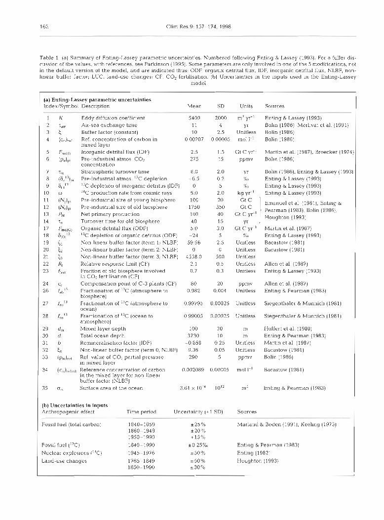
Table 1 (a) Summary of Enting-Lassey parametric uncertainties. Numbered following Enting & Lassey (1993). For a fuller discussion of the values, with references, see Parkinson (1995). Some parameters are only involved in one of the 5 modifications, not in the default version of the model, and are indicated thus: ODF, organix detrital flux; IDF, inorganic detrital flux; NLBF, nonlinear buffer factor; LUC, land-use changes; CF, CO2 fertilisation. (b) Uncertainties in the lnputs used in the Entlng-Lassey

model

(a) Enting-Lassey parametric uncertainties Index/Symbol Description Mean Units Sources

1 K Eddy diffusion coefficient 5400 m2 yr-' Enting & Lassey (1993)

yr Bolin (1986), Merlivat et al. (1991) Unitless Bolin (1986) m01 l-' Bolin (1986)

Air-sea exchange time 11 Buffer factor (constant) 10 Ref. concentration of carbon in 0.00207 mixed layer Inorganic detrital flux (IDF] 2 5 Pre-industrial atmos. COz 275 concentration Stratospheric turnover time 6.0

Gt C yr-' Martin et al. (1987), Broecker (1974) ppmv Bolin (1986)

yr Bolln (19861, Enting & Lassey (1993) 'L Enting & Lassey (1993) O r Enting & Lassey (1993)

kg yr-' Enting & Lassey (1993)

Pre-industrial atmos. I3C depletion -6.5 I3C depletion of inorganic detritus (IDF) 0 14C production rate from cosmic rays 6.0

11 ( N ) Pre-industrial size of young biosphere 100 12 (N,,),, Pre-industrial size of old biosphere 1750 13 PN Net primary product~on 100

Gt C Emanuel et al. (1981), Enting &

G t c I Pearman (1983), Bolin (19861, G t C Houghton (1993)

Yr Turnover time for old biosphere 40 Organic detrital flux (ODF) 5 0 I3C depletion of organic detritus (ODF) -24 Non-linear buffer factor (term l ; NLBF) 59.56 Non-linear buffer factor (term 2; NLBF) 0 Non-linear buffer factor (term 3; NLBF) 4558.0 Relative response limit (CF) 2.1 Fraction of old biosphere involved 0.7 in CO2 fertilisation (CF) Compensation point of C-3 plants (CF) 80 Fractionat~on of 13C (atmosphere to 0.982 biosphere) Fractionation of 13C [atmosphere to 0.99795 ocean) Fractionation of I3C (ocean to 0.99005 atmosphere) Mixed layer depth 100 Total ocean depth 3730 Remineralisation factor (IDF) -0.858 Non-linear buffer factor (term 0; NLBF) 9 36 Ref. value of CO2 partial pressure 290 in mixed layer Reference concentration of carbon 0 002089 in the mixed layer for non-linear buffer factor (NLBF)

Gt C yr-l Martin et al. (1987) 1C Enting & Lassey (1993)

Unitless Bacastow (1981) Unitless Bacastow (1981) Unitless Unitless Allen et al. (1987) Unitless Enting & Lassey (1993)

ppmv Allen et al. (1987) Unitless Enting & Pearman (1983)

Unitless Siegenthaler & Munnich (1981)

Unitless Siegenthaler & Munnich (1981)

Hoffert et al. (1980) Enting & Pearman (1983) Martin et al. (1987) Bacastow (1981) Bolin (1986)

m m

Unitless Unitless

PPmv

Bacastow (1981)

m2 Enting & Pearman (1983) 35 G,, Surface area of the ocean 3.61 X l0l4

(b) Uncertainties in inputs Anthropogenic effect Time period

Fossil fuel (total carbon) 1840-1859 1860-1949 1950-1990

Foss11 fuel (I3C) 1840-1990

Nuclear explosions ("C) 1945-1976

Land-use changes 1765-1849 1850-1990

Uncertainty (? 1 SD) Sources

*25% Marland & Boden (1991), Keeling (1973) * 2 0 9'0 *15%

*0.25% Enting & Pearman (1983)

*50% Enting (1982)

+50% Houghton (1993) +30%

Parkinson & Young: Uncertainty and sensitivity in carbon cycle n~odelling 163

the amounts of carbon in the atmosphere and the biosphere taken from observations; whilst those for the ocean are calculated by integrating the model equations until the ocean comes into equilibrium with the rest of the system.

The next step in MCS analysis is to construct the pdf's for the parameters and inputs of the model. Dur- ing each MCS realisation, the random selections of the parameter and input values are treated differently. For the parameters, the value is chosen at the start of the realisation and held constant during the realisation; whilst for the inputs, the value is chosen randomly at each time step during each realisation. This is because the parameters are considered to be constant during the whole realisation; whereas the inputs are assumed to be time series that vary continuously in a stochastic manner over the specified simulation interval. Nor- mally, this means that they are defined either as: deterministic or measured inputs, to which random noise with a specified pdf is added (this is the approach used here); or as time series generated by models such as a Autoregressive (AR), Autoregressive Integrated Mov- ing Average (ARIMA), or Transfer Function (TF) models with deterministic and stochastic inputs. Such time series models are obtained usually from the analysis of the available observational data, using statistical methods of identification and parameter estimation (see e.g. Box & Jenkins 1970, Young 1984). In all these cases, however, the basic stochastic inputs that drive the time series models are zero mean, serially uncorre- lated random variables ('white noise') with specified pdf's.

Table 1 summarises the means and standard deviations (under a Gaussian pdf assumption) of the parameters and inputs used in the MCS analysis. It is important to realise that all the model parameters and inputs are expressed in stochastic form in order to carry out a complete analysis. Note also that these statistical measures are derived as objectively as possible from independent sources, i.e. they are a priori values. Model parameter estimation (sometimes termed 'model optirnisation', 'calibration' or 'fitting'), i.e. the systematic adjustment of the parameter values so that the model is in better agreement with observations (see later), is not carried out until it has been established whether the a prionmodel structure is a reasonable representation of the 'real world'.

The number of stochastic realisations, n, needed for the MCS analysis is defined by the K-S statistic, i.e.

where K, (for a confidence level a) is read from statistical tables, and d is the level of difference allowed between 2 cfd curves before it is considered 'signifi-

cant' (see e.g. Spear 1970). For the EL model, the difference is considered significant if the means or standard deviations of histograms from 2 CO2 responses are different by more than 5% of the change in the mean CO2 level over the simulation period. Since the change of the mean level over the simulation period is approximately 80 ppmv, therefore, the cfd curves must differ by more than 4 ppmv for significance. In this situation, we find that 160 realisations are needed in order to detect a 'significant' difference. (For full details of this methodology, see e.g. Parkinson 1995.)

GSA is a special, Monte Carlo-based method which provides a means for objectively determining which of the model parameters have the most significant effect on a particular aspect of the model behaviour over the specified simulation period. Here, a range of 'acceptable' behaviour is first defined for each model output. Then, if any of the outputs from a given realisation fall outside their respective ranges, this realisation and the model parameters which produced it are considered as 'unacceptable' representations of the system. In this manner, the parameter values which lead to such unacceptable behaviour are classified as part of the 'not behaviour' (B) set; whilst those which result in acceptable response characteristics are classified as part of the 'behaviour' (B) set. Thus, the results from n realisations produces nb values for each parameter in the B set and (n - nb) values in the B set. For each parameter, K-S statistics are then used to find if there is a significant difference between the values in the B and B parameter sets (an example is given in Fig. 3) . This information is valuable in many ways; for instance, it

Atmospheric C& Conccnrra~ion (ppmv)

Fig. 3. Typical example of Kolmogorov-Srnirnov statistics applied to the results of Monte Carlo Simulation. The solid line and dashed line show the cfd curves obtained from 2 versions of the Enting-Lassey model, whilst the dot-dashed line shows the magnitude of the difference between these 2 curves. Since this difference never exceeds the level of significance (dotted line), the 2 versions are said to be 'not significantly different'. The curves could equally be from (a) a model and observations, or (b) 2 parameter sets, one of

'acceptable behaviour' and the other not-see Section 3

164 Clim Res 9:

reveals those parameters which are most important in defining the specified behavioural pattern, and steps can be taken to reduce the uncertainties associated with these most sensitive parameters. It can also suggest those (normally few) physical mechanisms in the simulation model that are most important in defining given behavioural phenomena and, conversely, those aspects of the model which appear to play little part in defining such behaviour.

The bands of acceptable behaviour are defined with reference to the observational record. Initially, in the case of the EL model, the 95 % confidence limits associated with the observed atmospheric CO2 concentrations (see Table 2) were used in this regard. However, it was found that these bands are so narrow compared with the range of uncertainty generated from the MCS that very few realisations exhibited the behaviour, i.e. nb was quite close to zero. Statistical analysis of such small sample sizes is naturally unreliable and so some way is needed to increase the number of acceptable realisations. One approach is to increase the width of one or more of the acceptability bands and, in this case, a 5-fold increase in all the bands yields usable results. While this is a fairly crude adjustment, it still allows for discrimination between parameters which have a relatively large effect on the model and those that do not. More rigorous enlargement of the 'behaviour space' can be achieved using more complex 'parameter space adjustment' techniques (see e.g. Keesman 1990 and Keesman & van Straten 1990) but these were not utilised in the present preliminary study.

Finally, Stochastic Model Optimisation can be carried out using MCS. We propose this as a first stage in model optirnisation and fitting, to be carried out only after the efficacy of the model structure has been confirmed. It is achieved by systematically adjusting the complete pdf's (i.e. the means and variances in the Gaussian case considered here) of the statistically significant parameters, as indicated by the GSA, to produce a model which yields the highest number of acceptable behaviour (B) realisations. For simplicity, in this paper, only the means of the pdf's for the most significant parameters have been utilised for optimisation, with the variances kept constant. However, this still yields interesting results and suggests strongly that certain of the a prioriassumptions about important parameter values should be investigated.

4. SELECTION OF PARAMETERIC UNCERTAINTY LEVELS IN MCS

One of the most difficult and challenging aspects of MCS analysis applied to large deterministic models is the selection of the uncertainty levels, particularly the

definition of pdf's for the model parameters. In this section, we discuss the issues involved in this process and seek to justify the approximations utilised in the paper to circumvent these difficulties. Bearing in mind the possible effects of these approximations, we also stress that the results of the subsequent MCS analysis must be considered carefully, taking into full account the points raised in this section.

The distributions should reflect the combined uncertainty associated with the system, as perceived by the scientific community, and we have obtained them as objectively as possible from many sources, such as published observations, calculations from independent modelling exercises, and the opinions of experts in the field (these sources are indicated in Table 1; full details are given in Parkinson 1995). However, since there is no truly objective method for carrying out this aspect of the analysis, certain assumptions have to be made about the nature of the pdf's. Some research workers in the area (e.g. Oeschger et al. 1975, Siegenthaler & Oeschger 1987, and subsequent studies used as a basis for IPCC 1996) have suggested that there is a high degree of correlation between several parameters, most notably the vertical diffusion coefficient K and the gas exchange coefficient K. However, these papers only provide very limited information in this regard and certainly do not allow for the specification of a complete covariance matrix of the type required for MCS under the assumption that the model parameters come from a multivariate Gaussian distribution. More- over, it should be noted that these previous studies have used box-diffusion models similar to that considered here and so their results are not independent sources within the requirements of our study. In particular, since we are intending to assess the suitability of the a priori model structure, we would run the risk of using circular arguments.

With these observations in mind, we have reluctantly assumed that the parameters each come from independent Gaussian distributions defined by the mean values and variances obtained in the manner described above (although any other distribution could have been used, and a uniform distribution might be better justified in certain circumstances). In MCS terms, this means that the parameter values for each stochastic realisation are drawn at random from a multivariate Gaussian distribution defined by the vector of mean parameter values and an associated, purely diagonal, covariance matrix with the assumed variances on the diagonal, and zero covariance elements.

This assumption of statistical independence is, of course, a potentially limiting one, since the computed uncerta~nties in the MCS analysis will yield different results from those obtained if the parameters had non- zero covariances. However, these are only initial

Parkinson & Young: Uncertainty and sensitivity in carbon cycle modelling 165

assumptions and, if better data and other independent information become available, they can be adjusted as necessary. Moreover, in an attempt to address this potential problem, we have considered the effect on the MCS results of reducing the a priori variances associated with the independent parametric pdf's. Our reasoning in this regard is based on the fact that the assumption of statistical independence is equivalent to considering a probability ellipsoid in the associated parameter hyper-space, whose axes are aligned with the axes of the space, and whose major and minor diameters are dependent upon the assumed variances of the individual parameters. If the parameters are not independent, however, this ellipsoid becomes both differently oriented and shaped because of the non-zero covariances. In particular, the existence of relatively large covariance elements can result in an ellipsoid with large differences between the major and minor diameters and, in the limit, the parameters concerned become linearly dependent and lie on a hyper plane. A simple illustrative example is discussed in Appendix 1.

Although it is impossible to evaluate directly how valid this approximate approach to pdf selection may be in the case of the full EL model, we have been able to investigate its consequences in relation to the reduced-order differential equation model approximation to the EL model, as obtained by the DMA mentioned in the 'Introduction' (see Young & Parkinson 1996, Young et al. 1996). These references show that this fourth order, linear differential equation approximation (3 dominant modes plus an integrator to account for mass conservation), which is obtained by referring only to the unit impulse response of the EL model, yields an atmospheric CO2 response to the fossil fuel input record which is almost identical (99.99% of the response explained) to that of the full nonlinear EL model over the whole of the historical period, 1840 to 1990. Just as importantly for our present purposes, since DMA is based on statistical estimation, it yields the estimates of the reduced-order model parameters and their associated covariance matrix. Conse- quently, it is possible to compare the results obtained from MCS analysis applied to the reduced-order model using both this full covariance matrix and its diagonal approximation.

The reduced-order differential equation model has 7 parameters and the off-diagonal elements of the 7 X

7 dimensional covariance matrix are relatively quite large, with the 2-dimensional projections of the associated probability ellipsoid indicating high levels of correlation between the estimates. Despite this, however, the MCS results obtained using the purely diagonal approximation to the covariance matrix, with no reduction in magnitude, produce a lower variance ensemble of atmospheric CO2 responses than those obtained

using the full matrix above. On average, over a simulation period between 1840 and 2100, the standard deviation of the ensemble about the mean response is 60 O/u of that in the full matrix case (varying from approximately 100 % between 1840 and 1940 to 30 % between 2090 and 2100). In other words, the diagonal approxi- matlon, which assumes independence in the parametric uncertainties, actually underestimates how the effects of this uncertainty propagate through the system.

Although the full EL model may well not behave in a similar manner to the reduced order model in MCS analysis, these results show that utilising a diagonal approximation to the covariance matrix does not nec- essarily amplify the effects of parametric uncertainty. In particular, it cannot be assumed that such an approximation will result in more volatile and sensitive ensemble MCS responses than would have been obtained if the full covariance matrix had been known and employed. For this reason, we believe that our approximate approach can be justified, particularly since we also present the results obtained with a reduction in the magnitude of the elements in the diagonal approximation of the covariance matrix (i.e. a reduction in the assumed uncertainties of the model parameters) and issue strong caveats about the interpretation of the results.

5. RESULTS FROM THE MONTE CARLO SIMULATION ANALYSIS

This section presents the results of the uncertainty and sensitivity analysis for the EL model. In Sub- sections 5.1 and 5.2, the comparative results from a number of different versions are discussed but, because the sensitivity analysis is very time consum- ing, the remaining Sub-sections 5.3 to 5.5 are concerned only with version E29 (described below). This version was selected for these more detailed studies since its total carbon response matches the independent observations better than any of the other versions. In addition to the analysis outlined in Section 3, Sub- section 5.5 presents some 'predictive' results obtained by simulating the model into the future using an IPCC scenario, and then compares the resulting uncertainty with that found in alternative deterministic studies. It should be noted that, following normal convention, the uncertainties in all the results presented here relate to the 95 % confidence limits (+2 standard deviation^).^

3Note that this is not the same as the presentation of parameter and input uncertainties (Table l), which quote 66% confidence limits (*l standard deviation) following Enting & Lassey (1993) and Enting & Pearman (1983)

166 Clirn Res 9: 157-174. 1998

I (I.) 6:'. the rtmorpherir IJC depletion

- >

5 400 0 9

2 350 c 0 a

2 3oo U C

r 4

2 250 - <

-15001 1800 1850 1900 1950 2000

Year

(a) PO, I h c atmospheric CO2 concentratiorl

-

-

..................................................

+ +W+ + ............ ...... ........... .. .....................

Fig. 4. Evolution of the stochastic uncertainty of the 3 outputs of Enting-Lassey model version E29. Statistical comparison is carried out at last point on the graph. The mean variation is shown as a full line and the dashed lines are the 95% confidence limits. Crosses are observational data: in (a), the observational data are from Friedli et al. (1986) and Enting & Lassey (1993); in (b), from Friedli et al. (1.986) and Enting &

Pearrnan (1983); In ( c ) , from Enting & Lassey (1993)

5.1. Stochastic simulation results

Simulating the EL model over the industrial period yields the graphs similar to those presented in Fig. 4. While these show the evolution of the stochastic uncertainty for model version E29 alone, the results for all the other model versions a re qualitatively very similar. Observational data are also shown on these graphs as

Table 2. Comparison of the MCS results of Enting-Lassey model versions E19 and E29, to observat~ons. Date given as

year and decimal fraction of year

Output Date Model response Observed (with 95 % conf.) response E19 E29 (with 95 % conf.)

crosses, for comparison. Table 2 compares the MCS results of model versions E19 (which includes the organic and inorganic detrital fluxes, and CO2 fertilisation) and E29 (which includes both the detrital fluxes, CO2 fertilisation, and land-use changes) with the observations at the end of the simulation period. The E19 model results a re shown here because its 13c response is closest to the observations; whilst, in the case of the E29 model, the total carbon response matches the observations very well. However, none of the model versions yield results that are very similar to the observed 14C m e a s ~ r e m e n t s . ~

The most obvious thing to note about the results in Table 2 and the associated results obtained with other model versions is the much smaller level of uncertainty in the observed values compared with that generated by the MCS analysis. For p, and the MCS uncertainty is about 20 times larger than that in the observations; whilst for &l3, the factor is about 6. This comparison must be treated with caution, however, since the model is sensitive to the uncertainty in the parameters which define the pre-industrial levels of total carbon, 'v and I4C (see Section 5 . 3 1 ~ and these are rather more uncertain than the present day levels. Neverthe- less the discrepancy is still very large and it seems unlikely that this is the only reason for the major differences revealed in Table 2.

There is clearly a large difference between the stochastic model results for I4C enhancement and the appropriate observations. The major problem appears to lie in the assumed mean parameter values. These are based on published values but they are rather different from those obtained by Enting & Lassey (1993), which are estimated using constrained numerical optimisation of the parameters in the model (see comments

41t IS interesting to note that the budgeting of I4C in global carbon cycle models is currently a controversial area (see e.g. Hessheirner et al. 1994)

'The pre-industrial levels of total carbon and are defined explicitly; that for '''C is calculated using other parameters, e .g . I4C production rate

Park~nson & Young: Uncertainty ar id sensit~vity in carbon cycle modelling 167

in the 'Introduction'). In order to maintain objectivity, however, we did not use these latter values, since they related specifically to exercises in model optimisation applied to the model under study, i.e. an assumption has been made that the a priori model structure is valid. Rather, we wished here to investigate the stochastic behaviour of the model using those parameter values which were considered by scientists to be most appropriate from a purely physical standpoint. This, we believe, is the major role of MCS in simulation model evaluation.

Following a request by I. G. Enting, however, we repeated the analysis using the EL constrained optimisation parameters (i.e. estimated means for cosmic ray production of I4C of 5.2 kg yr-l rather than 6.5 kg yr-l; and a conversion factor for nuclear weapons input of 2.8 kg kt-' rather than 4.5 kg kt-l). Not surprisingly, this yields figures for A , ' ~ of 188 + 3 6 9 % ~ that are much closer to the observed but still retain the significantly higher 95 % confidence interval observed in the previous simulation exercises. While these results confirm the efficacy of the Enting & Lassey constrained parameter optimisation, they also suggest that more consideration should be given to the reasons for the differences between the optimised parameter values and the prior published values (see the later discussion in Sec- tion ? on the problems of scale in defining environmental model parameter v a l ~ e s ) . ~

5.2. Statistical comparison of modified versions of the EL model

Statistical comparison between the MCS results of all 32 versions of the EL model show that neither of the oceanic detrital fluxes has any significant effect on p, and &,l3; but together they have an effect on the level of Inclusion of a nonlinearly varying buffer factor, as opposed to a constant value, has a significant effect on &l3, but not the other 2 outputs. Finally, land-use changes and CO2 fertilisation, both individually and in combination, make a significant difference to p, and &,l3, but not to Clearly, since all modifications have a statistically significant effect on at least one of the outputs, we cannot reject any as being redundant.

"t is interesting to note that recent work, published while the present paper was being reviewed (Lassey et al. 1996), uses the EL model with mean parameter values (particularly for the eddy diffusion coefficient K and stratospheric turnover time 7,,) based on more recent observations. This produces significantly better agreement with 14C observations and tends to confirm our comments

At this point, it is interesting to consider why the 3 outputs are affected significantly by different model modifications. Many of the reasons for this are appar- ent from considering the basic assumptions behind the EL model, and thus will not come as a surprise to global carbon cycle modellers:

(1) The inclusion of the oceanic detrital fluxes acts to Increase the flow of carbon from the ocean's surface layers to the deep layers. Together, they have a significant effect on the level of I4C in the atmosphere, but not on the levels of total carbon or I3C. It is likely that this is due to the changes that these fluxes would cause in the pre-industrial level of I4C, which is not fixed, unlike the pre-industrial levels of the other 2 outputs.

(2) The adjustment of the buffer factor from a constant to a nonlinear relation causes a reduction in the air-to-sea flux with increasing atmospheric levels. The main reason why this study found only &,l3 to be significantly affected is because the other outputs were not perturbed far enough away from their equilibrium points: larger perturbations to the model would lead to the nonlinearity having a larger (and eventually significant) effect. The greater uncertainty in p, and A , ' ~ probably helped to contribute to masking any differences.

(3) Land-use changes constitute an input of carbon to the atmosphere, whereas CO2 fertilisation acts as an output. In combination, they nearly cancel each other out; nevertheless, individually or together, they still have a significant effect on the atmospheric levels of total carbon and I3C. The fact that the 14C level is not significantly affected is because the atmospheric box has the same '"/C ratio as the biosphere, which is deliberate and is based on observations.

Obviously, many of the reasons for the presence or absence of a significant effect of a given modification on the outputs are intended and so, in this case, the statistical comparison of model versions has yielded little new information. Nevertheless, we have shown how this methodology can be used to clarify how a model is operating.

It is also important to point out here that the significance or otherwise of a modification depends on the choice of the outputs, simulation period and the point during the simulation at which analysis is carried out. Further, various modifications made to global carbon cycle models are carried out because of their perceived importance in determining future effects; consequently, if there is a lack of significant information on these effects in past observations, then they will be rejected by an analysis such as ours. Nevertheless, if this analysis is carried out carefully, it can help in deciding whether there is sufficient justification for the inclusion of a given modification.

Clim Res 9: 157-174, 1998

Table 3. Significant parameters of EL model version E29, found using GSA

Significant parameters K-S result

W '"C production rate from cosmic rays 0.325 (Sal3),, Pre-industnal atmos, 13C depletion 0.297 ( N o ) Pre-industr~al size of old biosphere 0.295 ( p ) Pre-industnal atmos. CO2 level 0.226 PN Net primary production 0.214 ram Air-sea exchange time 0.191

-

5.3. GSA and the evaluation of 'significant' model parameters

The results of the GSA analysis applied to EL version E29 are summarised in Table 3. In testing for 'significant' parameters, the K-S statistics assign a value between 0 and 1 to each parameter: the higher the value, the more significant the parameter is in determining whether the model response is 'acceptable'. The level of statistical significance in this case is 0.161. As can be seen, the 14C production rate from cosmic rays, o, is the most significant parameter. This is not surprising since, as pointed out in Section 5.1, its value makes a considerable difference as to whether the 14C model response is close to the observed level or not. The significance of the pre-industrial levels of CO2 and I3C are also to be expected since their uncertainties are much wider than the present day levels used for comparison, and so variation in their values would change the model response noticeably. However, the presence of the other 3 parameters [the pre-industrial size of the old biosphere, (No),,; the net primary production, PN; and the air-sea exchange time, z,,] is not so obvious. Again, it is likely that their significance is due to their comparatively high levels of uncertainty, but it is also possible that the processes they represent are more important in determining atmospheric CO2 levels than other parts of the model. This shows the potver of this method in picking up less obvious sources of model sensitivity.

5.4. Stochastic Model Optimisation

Approximate stochastic optimisation of EL version E29 is carried out by varying the means of the pdf's of the 6 most 'significant' parameters found using GSA (Table 3) . Parameter interaction was suspected between (p,),, and (6,'3)pi, the pre-industrial levels of total carbon and I3C in the atmosphere; and also between (NJPi, the pre-industrial size of the old biosphere, and PN, net primary production. The former interaction is

C-13 Deplerion (%o) v--

-7 -- 240 Carbon Dioxidc (ppmv)

Fig. 5. Variation of the probability of acceptable behaviour with the means of the pdf's of (p,),,, the pre-industrial atmospheric CO2 concentration, and (tiat3),,, the pre-industrial atmospheric I3C depletion, for Enting-Lassey model version

E29. (Default values shown by dashed lines)

confirmed, whilst the latter is denied by the application of analysis of variance (ANOVA) t e ~ t i n g . ~ By plotting graphs of the variation of the means of the pdf's versus the probability of behaviour [see, for example, Fig. 5 which shows a surface plot of (6,13)pi and (p&], it is found that a relatively high probability of acceptable behaviour is obtained by using the default means of parameters (p,),,, o and PN. However, T,, (No)pi and (S,'3)pi need to be adjusted quite considerably (by around 2 standard deviations) to yield optimum (or even near optimum) results. Parameter mean values that produce the approximately optimum (or near optimum) model in this stochastic sense are given in Table 4.

Also shown in Table 4 , for comparison, are the results of the deterministic, constrained 'least squares' model optimisation carried out by Enting & Lassey (1993). As can be seen, there is some difference between the 2 sets of results. In part, however, this is due to the differences in default values used by the 2 methods. For example, in the case of (pJpi, there is very little change between the default and optimal means in both cases; and for z,,,, the changes are of similar magnitude. The differences are more marked in the cases of (Sat3),, and o, which again emphasises our earlier conclusion that the model is somewhat questionable in its ability to model the minor isotopes of carbon. Comparison for the parameters (No)pi and PN

?If the output distributions and parameters distributions are Gaussian, as found with these models. ANOVA tests can be carried out to discover any interactions between significant parameters. If any distribution is not Gaussian, interaction can only be surmised

Parkinson & Young: Uncertainty and sensitivity in carbon cycle modell~ng

Table 4. Comparison of the results of stochastic model optimisation (this paper) with deterministic 'least squares' optinlisation (Enting & Lassey 1993) for the Enting-Lassey model

Parameter Units Constrained stochastic Constrained least squares model optimisation model optimisat~on

Optimal meand Default mean Optimal mean Default mean -

(PJp, PPmv 275 (270-295) 275 285.3 285 (LIJ)pi YW -6 1 (< -6.2) -6 5 -6.41 -6.5 =*m Y r 7.0 (6.5-8.5) 11 0 8.58 12 o kg yr-l 3.0 (2.6-4.6; 5.9-6.1) 6.0 5.15 6

(No)pl Gt C 2600 (2250-2800) 1750 b 1400

PN Gt C yr.' 180 (85-105; 175-195) 100 b 100

*Figures in parentheses show the ranges of values of parameter means whose probabilities were greater than 80% of the optimal value. bThese parameters were fixed during the deterministic model opt~rnisation

is rather academic since these parameters are frozen at the a priori assumed values in the constrained optimisation. However, the comparatively large changes which lead to the optimal values in the unconstrained stochastic case considered here rather call into question Enting & Lassey's decision to constrain them.

To summarise, the probability of acceptable behaviour in model version E29 is approximately doubled by adjusting the means of the pdf's associated with several of the significant parameters. Moreover, to achieve this high level of probability, relatively large changes, of around 2 standard deviations (i.e. to the edge of the 95 % confidence interval), need to be made to certain of these parameters. Comparison of these results with those obtained using deterministic optinlisation reveal some sirn- ilarities, with the main differences being due to parameters concerned with the minor isotopes. These results again serve to emphasise the possible shortcon~ings of

Year

Fig. 6. Evolution of stochastic uncertainty of atn~ospheric carbon dioxide concentration of Enting-Lassey model version E29 forced by IPCC scenario IS92a. Dashed lines are uncertainty bands (95% confidence limits) of the original sirnula- tion. Dot-dashed lines are the 95% confidence limits of the simulation with parametric and input uncertainties halved and constrained to the observed CO, level in 1990 [method

(3) -see Sechon 4.51

E29 in its modelling of I3C and 14C. It must be remem- bered, however, that the stochastic model optinlisation used here is still quite crude and so conclusions based on it are fairly speculative at this stage.

5.5. Uncertainty in future projections of CO2 levels

The final set of MCS results are obtained by extend- ing the time period of interest up to the year 2100 in order to provide data pertaining to the debate on anthropogenic climate change. Extra model inputs for fossil fuel and land-use changes during this time span are based on the IPCC scenario IS92a (IPCC 1992). It must be emphasised that version E29 is used with its original, a priori, pdf's, rather than either the optimised values discussed in the previous Section 5.4 or those of Enting & Lassey. This is in line with our previous concentration on the a priori parameter values considered by scientists to be most appropriate from a purely physical standpoint, but it is also because the model incorporating the adjusted values has not been vali- dated against independent data.

Fig. 6 shows the stochastic evolution of the atmospheric CO, concentration, p,, produced by E29 between 1990 and 2100.' The dashed lines show the uncertainty (95% confidence limits) in the evolution, which grows steadily throughout the simulation period from 351 i 43 ppmv in 1990 to 664 +. 144 ppmv in 2100. Since the assumption of parametric independence is

'In this study, it is assumed that there is an uncertainty of 25% in converting a political scenario, such as IS92a, into yearly fossil fuel emissions and of 50 % in converting it into land-use change flux. However, the simulation was repeated with zero uncertainty on these 2 inputs between 1990 and 2100, and no significant reduction in the output uncertainty occurred

170 Clim Res 9: 157-174, 1998

potentially controversial and may (but does not neces- sarily; see earlier discussion in Section 4) lead to over- estimation of this future uncertainty, the MCS was also carried out a further 3 times under different conditions: (1) with parametric and input uncertainties reduced by an arbitrary factor of two9; (2) with each realisation constrained to the uncertainty in the observed CO2 level in 1990 (353 + 2 ppmv); and (3), with a combination of both (1) and (2). Simulation (3), which grows from 353 * 2 ppmv in 1990 to 669 * 48 ppmv in 2100, is shown by the dot-dashed lines in Fig. 6. Of the three, this method naturally produces the output evolution with lowest level of uncertainty.

Finally, in Table 5, the results of the above 4 stochastic simulations are compared with those from 3 deterministic modelling exercises, including those of IPCC (1995)1°. It is clear that the uncertainty produced by the MCS analysis is much larger than that arising from the deterministic methods; in particular, the level of output uncertainty generated by using the original parametric and input uncertainties is between 5 and 10 times larger. Even when we consider the stochastic simulation with the narrowest output uncertainty (method 3). which will probably attract the least criticism from global carbon cycle modellers, these bands are still 50% wider than the widest of the deterministic results. It is likely that this difference would be larger still if the stochastic methodology was to be applied to a range of global carbon cycle models, as in the deterministic IPCC simulation studies.

6. LIMITATIONS OF THE ANALYSIS

Evaluating the effects of uncertainty on a fairly complex, deterministic simulation model is beset with many difficulties and it is important that the limitations of the analysis carried out in this paper should be taken fully into account when evaluating the results presented in previous sections. In this regard, the following points should be noted.

(1) In the absence of independent evidence to the contrary, the assumed probability distribution func-

'A consequence of this is that the uncertainty (66'Yo confidence limits) of the pre-industrial level of CO2, (p,),, is thus reduced from 275 & 15 ppmv to 275 * 7.5 ppmv which is closer to the uncertainty discussed in Schimel et al. (1995)- a value published too late to be considered explicitly by this analysis

''The uncertainty in each of the deterministic exercises is due to the following: Schimel et al. (1995), variation between different models; Wigley & Raper (1992), variation in one model due to different assumptions about feedbacks; Enting & Lassey (1993), parameter uncertainty constrained by observations

Table 5. Comparison of the uncertainty in future CO2 levels (in ppmv) due to IPCC scenario JS92a between 3 deterministic modelling exercises (Wigley & Raper 1992, Enting & Lassey 1993, Schimel et al. 1995) and the stochastic methods

used in this paper

Year Uncertainty in Source atmospheric CO2 Range Extent

2050 494 to 510 16 Sch~mel et a1 (1995)" 520 to 550 30 Wigley & Raper (1992) 491 * 86 172 This paper, orig. simulation 487 * 44 88 This paper, method (1) 497 * 37 74 This paper, method (2) 494 r 22 44 This paper, method (3)

2100 667 to 719 52 Schimel et al. (1995)d 740 to 800 60 Wigley & Raper (1992) 615 to 683 68 Enting & Lassey (1993) 664 + 144 288 This paper. orig. simulation 658 * 71 142 This paper, method (1) 674 * 84 168 This paper, method (2) 669 * 48 96 This paper, method (3)

dThe results presented in this paper are derived from Enting et al. (1994)

tions of the parameters and inputs are taken to be independent and Gaussian. These may well be flawed assumptions but it is difficult to use any others, given the possibility of circularity in selecting parametric values, as mentioned in Section 4. If new information were to become available, modifications to the analysis would be required. The choice of the means and standard deviations of the assumed probability distribution functions is also somewhat subjective; other researchers in this field may have rather different ideas of these values. If any of these possibilities are confirmed, then it is likely that the uncertainty associated with the Monte Carlo realisations could be different to that obtained in the present study.

(2) The definition of 'significance' associated with the MCS analysis is somewhat subjective; and again, other researchers may disagree with that used in the present paper

(3) For convenience in the present initial study, the model response has only been studied at one point during a 225 yr period. This may be unrepresentative, and so it would be better to consider several different years during the simulation; or, ideally, to evaluate the stochastic response at every annual step.

(4) Only 3 model variables have been considered as outputs; many more could be chosen and studied (including, perhaps, the model's eigenvalues); and such analysis may well yield other interesting results.

(5) The GSA has suffered from the large difference between the uncertainty in the model results and that in the observations. We chose to handle this by increas-

Parkinson & Young: Uncertdinty ai nd sensitivity In carbon cycle modelling 171

ing the width of the uncertainty bands on the data; on the other hand, it might have been better to reduce the uncertainty levels on the parameters, given the rather subjective nature of their specification and the potential problems of scale mentioned above. Improvement in the GSA analysis might also be achieved by using a more robust method, such as the 'set-membership' technique of Keesman & van Straten (1990).

We do not believe that these various limitations sen- ously affect the general conclusions derived from the analysis reported here, provided our caveats are heeded carefully. Neither do they lessen the useful- ness of the stochastic simulation approach, especially since the emphasis of most other studies in this area includes only deterministic sensitivity analysis, which is clearly less flexible and of more limited value than the stochastic alternative considered here. In many ways, our initial results are illustrative of what can be achieved by MCS/GSA analysis and a more detailed investigation of the EL and other global models is a logical next step, together with some refinement of the analysis in the light of the current results.

7. DISCUSSION AND CONCLUSIONS

With the advent of modern fast computers, MCS analysis now provides a simple and practical method for quantifying the effects of stochastic uncertainty in reasonably large and complex, nonlinear simulation models. The study of global carbon cycle modelling carried out in this paper has involved the application of such MCS analysis, and other methods of dynamic model evaluation, to scientifically acceptable models of global energy balance and the global carbon cycle (Parkinson 1995). A companion paper (Young et al. 1996) has concentrated on the methodological aspects of the study and its place within a framework of model building, which includes data-based modelling; while the present paper outlines the initial results obtained from the MCS studies, which have been concerned with the well known Enting-Lassey modified box-diffusion model of the global carbon cycle (Enting & Lassey 1993).

Although the main aim of this research has been to suggest and investigate a general MCS approach to evaluating the effects of uncertainty in global carbon cycle models, the results obtained from its application to the EL model have also provided interesting additional insight into the nature of this model and its potential utility in global climate studies. We have found that, whilst the EL model appears to simulate the movement of total carbon quite well using fixed parameter values, it is characterised by a relatively high degree of inherent sensitivity to uncertainty in some of

the parameter values. This tends to confirm the earlier results of Gardner & Trabalka (1985) using a different global carbon cycle model.

In addi t~on, the results of stochastic s~mulation projections up to the year 2100 yield a much wider uncertainty range than those obtained from deterministic modelling exercises using the same input scenarios. Even when the parametric and input uncertainties a re reduced by a factor of 2 (to account for possible correlation between parameters, a s discussed in Section 4) and the simulation is constrained to produce the observed CO2 level in 1990, the stochastic output uncertainty is still 50 % higher than the highest comparable estimate found using deterministic methods. While this level might be reduced if the EL model is constrained using the full CO2 history, it could be increased if the stochastic analysis were to be applied to other global carbon cycle models currently considered realistic (and used to produce the uncertainty estimate in Schimel et al. 1995). We believe that these results should at least be taken into account when evaluating such projections for policy purposes.

One reason why the EL model is sensitive to parametric uncertainty a t the levels used in our MCS analysis could be that the parameter values are based on indirect observations a t different scales to that on which the model is based-mainly local or regional field studies and/or laboratory measurements. It is certainly not obvious that parameters obtained at these smaller scales are completely relevant to those used a t a much larger scale, as in global simulation studies, and this may lead to incorrect estimation of the uncertainties involved at this larger scale. This probably accounts, at least in part, for the differences in the a priori assumed values for the parameters in the EL model and those obtained by model optimisation, whether deterministic (as in Enting & Lassey 1993) or stochastic (as in the present paper). We believe that this question of scale in global simulation modelling (or, indeed, in most other areas of environmental modelling) is most important, particularly with regard to the specification of parameter values. Certainly, it is deserving of much greater attention than it has received heretofore, given the importance of mechanistic simulation models in environmental research.

In the paper, MCS has also been used to evaluate whether the addition of extra complexity to the model makes a statistically significant difference to the model response. In this case, all 5 of the modifications suggested by Enting & Lassey, and considered in the present study, affect at least 1 of the outputs significantly, and so none a re rejected a s being redundant. On the other hand, it is important to note the results obtained when GSA is applied to the EL model version E29, whose response is closest to the observed CO2 levels.

Clim Res 9: 157-174, 1998

These show that, from over 20 parameters, only a few appear to have a statistically significant effect on the model output, implying that a reduction in the uncertainty of these significant parameters should be a prior- ity for improving the stochastic nature and reljability of the EL model. In particular, since the significance of the pre-industrial level of atmospheric CO2 in the present EL model concurs with a similar result obtained by Gardner & Trabalka (1985) using a different global carbon cycle model and a somewhat different type of stochastic sensitivity analysis, it is clear that this parameter is deserving of still greater attention in future studies.

These GSA results suggest that, while the EL model is a quite complex, high order set of nonlinear differential equations defined by a relatively large number of parameters, its dynamic behaviour is influenced mainly by a much smaller number of 'important' parameters. In addition, all of the MCS ensemble responses generated in our study have approximately Gaussian amplitude distributions and, since the parametric and input uncertainties are also Gaussian, this indicates that the nonlinear elements of the model are not being excited to any great extent. Such simplifying conjec- tures are supported by the results obtained from the novel dominant mode analysis reported in Young et al. (1996), where the whole topic of reduced-order models and domlnant mode behaviour is discussed in greater detail. These results suggest that the model behaviour is characterised by only a small number of dominant, linear dynamic modes, and that much of the inherent complexity of the simulation, including nonlinearity, is having only a small effect on the main model outputs over the historic period, where the model has been optimised in relation to observational data.

If they are confirmed by later, more detailed analyses, these model simplification results may have important implications for the interpretation of the long term predictions obtained from the EL and other similar models (e.g. the prediction of the future atmospheric CO2 concentrations well into the next century). For instance, if the nonlinearities in the model have not been activated sufficiently over the historical period, as our results suggest, then the constrained optimisation results obtained by fitting the model to data over this same historical period cannot be considered completely satisfactory in this regard. Consequently, any model predictions that are affected to any appreciable degree by these estimated nonlinearities must be seriously questioned before the predictions are utilised for other purposes. More generally, the implications of the uncertaint~es associated with all the parameters in the model, including those that are assumed known in the constrained optimisation exercises, must also be evaluated very carefully. In particular, their effect on the model predictions need.s to be acknowledged and

investigated fully before the policy implications of the predictive results can be properly evaluated.

Finally, it is important to stress that the above conclusions are based only on a preliminary study of the EL model. A great deal more analysis could be per- formed, following discussion of these initial results with experts on global carbon cycle modelling. It is felt that such further studies are essential before any firmer conclusions can be reached. In this regard, we hope that the results presented in this paper will help to stimulate further research on the effects of uncertainty in global climate models.

Appendix 1. Covanance matrices and probab~lity ellipsoids

Consider 2 Gaussian distributions with the same mean vector a, = [ l 0 20jTbut the following, different, covariance matrices

Since C, is diagonal, the parameter values drawn from this distribution are statistically independent; whereas in the case of CNl, the parameters are correlated because of the significant off-diagonal elements. In this case, by reducing the variances (i.e. the diagonal elements) in C, by a factor of 10, i t is possible to approximately inscribe the resulting smaller probability ellipse (in this 2-parameter space) withln the ellipse defined by C, , , so reducing the uncertainty in the region of the mean values to levels which are comparable with those defined by CN/ in this same central region.

In relat~on to the variance reduction exercises in the MCS analysis carried out in this paper, note the following comments:

(1) If the variance reduction reasonably achieves its objective, then the uncertainty injected into the system could be less than the actual, since parts of the 'true' hyper-ellipsoid are then not explored in the MCS analysis. In other words, the analysis in this situation might even be conser- vative and so underestimate the effects of uncertainty (see, for instance, the example in the main text where underestimation occurs even w~thout variance reduction)

(2) Although the region explored by the MCS is smaller if the variances are reduced, this exploration is still carried out under the assumption that the parameters are independent, which could possibly amplify the effects of uncertainty in this smaller reglon.

(3) The situation may well not be as bad as that in the simple example above, where the off-diagonal elements in CNI have been selected so that the parameters are highly correlated and the matrix is very near to singularity (which occurs when these elements are set to about 1.2649 and the 2 parameters become linearly dependent). If the off- diagonal elements are chosen as unity rather than 1.25, for example, then the 2 distributions cover quite similar regions of th(? parameter space. Of course, comment (2) still applies in this situation, so that the level of irnprove- ment will be a function of the unknown covanances and so is difficult to assess.

Parkinson & Young: Uncertainty and s e n s ~ t ~ v ~ t y in carbon cycle modelling 173

Acknowledgements. The authors are grateful to the UK Nat- ural Environment Research Council (NERC) for supporting the research reported in this paper by the award of a research studentship. We also thank Dr Ian Enting of CSIRO, Australia, for generously supplying the original code of the Enting- Lassey model and for providing valuable comments during the research study. The useful comments of the anonymous referees are also acknowledged.

LITERATURE CITED

Allen LH Jr, Boote KJ , Jones PH, Valle RR, Acock B, Rogers HH, Dahlman RC (1987) Response of vegetation to rising carbon dioxlde: photosynthesis, biomass and seed yield of soybean. Global Biogeochem Cycles 1 :l-14

Bacastow RB (1981) Numerical evaluation of the evasion factor. In: Bolin B (ed) Carbon cycle modelling: SCOPE 16. John Wiley & Sons. Chichester, p 95- 101

Bolin B (1986) How much CO, will remain in the atmosphere7 In: Bolin B, Doos BR. Jager J , Warrick RA (eds) The greenhouse effect, climatic change and ecosystems: SCOPE 29. Chap 3. John Wiley & Sons. Chichester

Box GEP, Jenkins GM (1970) Time series analysis, forecasting and control. Holden-Day. San Francisco

Broecker WS (1974) Chemical oceanography. Harcourt Brace Jovanovich, New York

Dowlatabadi H, Kandlikar M (1995) Key uncertainties in climate change policy: results from ICAM-2, 6th Global Warming Conference, San Francisco

Emanuel WR, Killough GEG, Olson J (1981) Modelling the circulation of carbon in the world's terrestrial ecosystems. In: Bolin B (ed) Carbon cycle modelling: SCOPE 16. John Wiley & Sons, Chichester, p 335-353

Enting IG (1982) Nuclear weapons data for use in carbon cycle modelling. Dlv~slon of Atmosphenc Physlcs, CSIRO, Mordialloc, Technical Paper 4 4

Enting IG, Lassey KR (1993) Projections of future CO2. Divi- sion of Atmospheric Research. CSIRO, Mordialloc, Tech- nical Paper 27

Enting IG, Pearman G1 (1983) Refinements to a one-dimensional carbon cycle model. Division of Atmospheric Research, CSIRO. Mordialloc. Technical Paper 3

Enting IG, Pearman G1 (1987) Description of a one-dimensional carbon cycle model calibrated using techniques of constrained inversion. Tellus 39B:459-476

Enting IG, Wigley TML. Heimann M (1994) Future emissions and concentrations of carbon dioxide: key ocean/atmosphere/land analyses. Dlvision of Atmospheric Research, CSIRO, Mordialloc, Technical Paper 31

Friedli H, Lotscher H, Oeschger H, S~egenthaler U , Stauffer B (1986) Ice core record of the 'v /l2C ratio of atmospheric CO2 in the past two centuries. Nature 324:237-238

Gardner RH, Trabalka JR (1985) Methods of uncertainty analysis for a global carbon dioxide model. Publication DOE/OR/21400-4. US Dept of Energy, Washington, DC

Hessheimer V, Heimann M. Levin I (1994) Radiocarbon evidence for a smaller oceanic carbon dioxide sink than previously believed. Nature 370:201-203

Hoffert MI, Callegari AJ, Hsieh CT (1980) The role of deep sea heat storage in the secular response to climatic forcing. J Geophys Res 85:6667-6679

Houghton RA (1993) The flux of carbon from changes in land use. In: Enting IG. Lassey KR (1993) Projections of future CO2, Appendix B. Division of Atmospheric Research, CSIRO, Mordialloc. Technical Paper 27

IPCC (1990) Climate change: the IPCC scientific assessment.

Houghton JT, Jenkins GJ, Ephraums JJ (eds). Cambridge University Press, Cambridge

lPCC (1992) Climate change 1992: the supplementary report to the IPCC scientific assessment. Houghton JT, Callender BA, Varney SK (eds). Cambridge Univers~ty Press, Cam- bridge

IPCC (1995) Climate change 1994: radiative forcing of climate change and an evaluation of the lPCC IS92 emission scenarios. Houghton JT, Meira Filho LG, Bruce J . Lee H. Callander BA, Haites E, Harris N, Maskell K (eds). Cam- bridge University Press, Cambridge

IPCC (1996) Climate change 1995: the science of climate change-contribution of Working Group 1 to the second assessment report of the Intergovernmental Panel on Cli- mate Change. Houghton JT, Meira Filho LG, Callander BA, Harris N, Kattenberg A, Maskell K (eds). Cambridge Univers~ty Press, Cambridge

Keel~ng CD (1973) lndustrial production of carbon dloxide from fossil fuels and limestone. Tellus 25:174-198

Keesman K (1990) Membership-set estimation using random scanning and principal component analysis. Math Comput Simul32:535-543

Keesman K, van Straten G (1990) Set-membership approach to identification and prediction of lake eutrophication. Water Resour Res 26(11):2643-2652

Lassey KR. Enting IG. Grudinger CM (1996) The earth's radiocarbon budget. Tellus 48:487-501

Marland G, Boden T (1991) CO2 emissions-modern record. In: Boden TA, Serpanski RJ, Farrell MP (eds) Trends '91: a compendium of global change. Carbon Dioxide Informa- tlon and Analysis Center, Oak Ridge, TN, p 386-389

Martln JH, Knauer GA, Karl DM, Broenkow WW (1987) VER- TEX: carbon cycling in the northeast Pacific. Deep Sea Res 34:267-285

Merllvat L, Etcheto J , Boutin J (1991) CO2 exchange at the air- sea interface: time and space variability. Adv Space Res 1 l (3) 77-85

Oeschger H. Slegenthaler U , Schotterer U , Gugelrnann A (1975) A box diffusion model to study the carbon dioxlde exchange in nature. Tellus 27:168-192

Parkinson SD (1995) The application of stochastic modelling techniques to global climate change. PhD thesis. Lan- caster University

Scavia D (1993) Lake ecosystem modelling: uncertainty. In: Young PC (ed) Concise encyclopaedia of environmental systems. Pergamon Press, Oxford. p 318-320

Schimel D, Enting IG, Heimann M, Wigley TML, Raynaud D, Alves D, Siegenthaler U (1995) CO2 and the carbon cycle. In: Houghton JT, Meira Filho LG, Bruce J, Lee H, Callan- der BA, Haites E, Harris N, Maskell K (eds) Climate change 1994. radiative forcing of climate change and an evaluation of the IPCC IS92 emission scenarios. Cam- bndge University Press, Cambridge, p 35-71

Siegenthaler U, Munnich KO (1981) l3C/I2C fractionation during CO, transfer from air to sea. In: Bolin B (ed) Carbon cycle modelling: SCOPE 16. John Wiley & Sons, Chlch- ester, p 249-257

Siegenthaler U, Oeschger H (1987) Biospheric CO2 emissions

during the past 200 years reconstructed by deconvolution of ice core data. Tellus 39B:140-154

Spear RC (1970) The application of Kolmogorov-Renyi statistics to problems of parameter uncertainty in systems design. Int J Control 11(5):771-778

Spear RC (1993) Regional sensitivity analysis in environmental systems. In: Young PC (ed) Concise encyclopaedia of environmental systems. Pergamon Press, Oxford, p 476-479

174 Clim Res 9: 157-174, 1998

Spear RC, Hornberger GM (1980) Eutrophication in Peel Inlet 11: identification of critical uncertainties via generalized sensitivity analysis. Water Res 14:43-49

Whitehead P, Young PC (1979) Water quality in river systems: Monte Carlo analysis. Water Resour Res 15:451-459

Wigley TML, Raper SCB (1992) implications for climate and sea level of revised IPCC emissions scenarios. Nature 357: 293-300

Young PC (1983) The validlty and credibility of models for badly defined systems. In. Beck MB, van Straten G (eds) Uncertainty and forecasting of water quality. Springer- Verlag, Berlin, p 69-100

Young PC (1984) Recursive estimation and time series analysis. Springer-Verlag, Berlin

Young PC, Beven KJ (1994) Data-based mechanistic modelling and the rainfall-flow nonlinearity. Environmetrics 5. 335-363 (special issue on 'Environmental Time Series Analysis')

Editorial responsibility: Hans von Storch. Geesthacht, Germany

Young PC, Lees M (1992) The active mixing volume: a new concept in modelling environmental systems. In: Barnett V, Turkman R (eds) Statistics and the environment. Wiley, Chichester, p 3-43

Young PC, Minchin PEH (1991) Environmetric time-series analysis: modelling natural systems from experimental time-series data. Int J Biol Macromol 13:190-201

Young PC, Naughton JJ, Neethling CG, Shellswell SH (1973) Macro-economic modeling: a case study. In: Eykhoff P (ed) Identification and system parameter estimation. Else- vier, New York, p 145-165

Young PC. Parkinson SD (1996) Simplicity out of complexity in forecasting climate change. Tech Note No. 146, Centre for Research on Environmental Systems and Statistics, Lancaster University

Young PC, Parkinson SD, Lees M (1996) Simplicity out of complexity in environmental systems: Occam's razor revisited. J Appl Stat 23(2-3):165-210

Submitted: May 16, 1996; Accepted: September 22, 1997 Proofs received from author($): February 9, 1998

uncertainty and sensitivity in global carbon cycle modelling · uncertainty and sensitivity in...

Documents