sensitivity analysis of adsorption isotherms...
TRANSCRIPT
Twelfth International Water Technology Conference, IWTC12 2008 Alexandria, Egypt
1
SENSITIVITY ANALYSIS OF ADSORPTION ISOTHERMS SUBJECT
TO MEASUREMENT NOISE IN DATA
Karim Farhat 1, Mohamed N. Nounou
2 and Ahmed Abdel-Wahab
3
1 Student, Chemical Engineering, Texas A&M University at Qatar
E-mail: [email protected] 2 Assistant Professor of Chemical Engineering, Texas A&M University at Qatar
E-mail: [email protected] 3 Assistant Professor of Chemical Engineering, Texas A&M University at Qatar
E-mail: [email protected]
ABSTRACT
Reflecting the importance of adsorption as a major water purification method, the
main objective of this research was to perform a sensitivity analysis on some of the
common adsorption isotherms subject to measurement noise in data. Even though most
of adsorption isotherms have been derived based on theoretical assumptions about the
adsorption mechanism, they involve model parameters that need to be estimated from
experimental measurements of the process variables. Specifically, for the Langmuir
isotherm, which can be linearized in three forms, it was sought to determine which of
these three forms would give the highest accuracy of the adsorption model parameters
– maximum amount of adsorbate per unit weight of the adsorbent and the constant
related to the affinity between the adsorbent and adsorbate. Another objective was to
estimate the adsorption parameters using the nonlinear Langmuir model, and to
compare their accuracy to the ones estimated using the most accurate linear form.
Furthermore, it was desired to examine the effect of noise magnitude on the estimation
accuracy for the various Langmuir forms (linear or nonlinear) by varying the noise
variance and the magnitude of the adsorption parameters themselves. To achieve this
aim, MATLAB programming software was used for simulations. The results of this
work could be summarized as follows: One of the linearized forms of Langmuir model
showed normal distribution and provided most accurate estimation of both model
parameters. In addition, it was shown that when the noise content (standard deviation)
increased on the data, less accurate estimates were obtained for both adsorption
parameters. Finally, the estimation accuracy was more sensitive to the magnitude of
the affinity constant than to the maximum amount of adsorbate in adsorbent; larger
values of affinity constant result in higher estimation accuracy of both model
parameters.
Keywords: Langmuir, linearization, parameters, noise
Twelfth International Water Technology Conference, IWTC12 2008 Alexandria, Egypt
2
INTRODUCTION
During the last few decades and as industries were growing, significant pollution
problems rose up, and handling them became a major concern especially for scientists
and engineers. In specific, a great deal of attention has been given to water pollution
problems as they threat one of the most vital natural resources for human life. For
example, the removal of toxic heavy metals (such as Zinc, Nickel, and Lead) from
groundwater and wastewater has been approached by various works and studies,
taking into consideration the very serious implications that these pollutants can have
on humans’ and other living beings’ health. Consequently, many water purification
methods has been developed and used to remediate consumable and waste water from
those pollutants. These methods include chemical precipitation (Hence [1]), reverse
osmosis (Ning [2]), electro dialysis, ion exchange, and finally adsorption.
In general, adsorption is a mass transfer process, which involves the contact of solid
called adsorbent with a fluid containing certain pollutants called adsorbate (Alkan and
Dogan [3]). These pollutants can be organic compounds, pathogens, and heavy metals.
And their contact with the surface of the adsorbent results in permanent bonds,
ensuring their removal from the fluid. The adsorption capacity depends on several
factors, such as the adsorbent type, its surface area, and its internal porous structure.
Additionally, since the attachment of the pollutant can be physical or chemical, the
physical and chemical structures as well as the electrical charge of the adsorbent can
significantly influence its interactions with the adsorbates, and thus the effectiveness
of pollutant removal.
Adsorption processes are characterized by their kinetic and equilibrium isotherms. The
adsorption isotherms specify the equilibrium surface concentration of the adsorbate as
a function of its bulk concentration. Several mathematical models have been proposed
to describe the equilibrium isotherms of adsorption. Some of the most popular models
include Langmuir, Freundlich, Redlich-Peterson, and Sips. A summary of these
isotherms is provided by Dabaybeh [4]. Even though most of these adsorption
isotherms were derived based on some theoretical assumptions about the adsorption
mechanism, they involve model parameters that need to be estimated from
experimental measurements of the process variables. Talking about Langmuir model
in specific, the isotherm has the following form:
e
ece
Cb
CbQq
1 (1)
where, eC is the equilibrium liquid phase concentration (mg/l), eq is the equilibrium
solid phase concentration (mg/g), cQ is the maximum amount of adsorbate per unit
weight of the adsorbent to form a complete monolayer, and b is a constant related to
the affinity between the adsorbent and adsorbate. In the above Langmuir model, cQ
and b are model parameters to be estimated from measurements of eq and eC .
Twelfth International Water Technology Conference, IWTC12 2008 Alexandria, Egypt
3
Unfortunately, measurements of the adsorption process variables, eq and eC , are
usually contaminated with noise or measurement errors due to random errors, human
errors, or malfunctioning sensors. The presence of such measurement noise, especially
in large amounts, can largely degrade the accuracy of the estimated isotherm
parameters, which in turn limits the ability of the isotherm to accurately predict the
adsorption capacity of a certain process. This is because most modeling techniques
estimate the model parameters by minimizing some objective function related to the
prediction errors of the model output ( eq ). Unfortunately, since the isotherm input and
output variables ( eq and eC ) are both measured, only minimizing the output prediction
errors may not lead to acceptable estimation.
Therefore, the objectives of this project were as follows:
1. Perform a sensitivity analysis to investigate the effect of the presence of
measurement noise on the estimation accuracy of the Langmuir model isotherms
(linear and non-linear). The effect of noise on the estimated parameters from each
of these linearized models was assessed, and recommendations on the best
linearized model were provided. Of course, the sensitivity analysis results will also
depend on the estimation method utilized.
2. Assess the effect of measurement noise on the parameters estimated from the
nonlinear Langmuir model and compare that to the effect on the parameters of the
most accurate linearized model.
3. Assess and compare the effects of different noise intensities and parameters (Qc
and b) magnitude on the latter’s accuracy estimation.
LITERATURE REVIEW
Being a major mass transfer process of multiple uses, researches continue about
adsorption process, its mechanisms, and its application in various fields. As it has been
noted, the basic concern of this study is to perform a general sensitivity analysis for
adsorption isotherms, using artificially added noise, to detect the best form of
Langmuir model for adsorption parameters’ estimation. In this regard, this study
intersects with some of the researches done before in the same field, while being
unique.
For example, the concept of comparing adsorption isotherms and parameters and
evaluating their accuracy by using different models has been discussed for: the
removal of selected metal ions by powdered egg shell (Otun et al. [5]), sorption of
organic compounds to activated carbons (Pikaar et al. [6]), adsorptive removal of
chlorophenols from aqueous solution by low cost adsorbent (Radhika and Palanivelu
[7]), removal of boron from aqueous solution by clays and modified clays (Karahan et
al. [8]), and many others. However, it is clear that these studies determine the best
fitting model only for the material, substance or process under study. Similarly, some
Twelfth International Water Technology Conference, IWTC12 2008 Alexandria, Egypt
4
studies determined the most suitable model to explain the adsorption process
depending on specific type of instrument used to get the experimental data; Modeling
in Adsorption-Desorption Noise in Gas Sensors Using Langmuir and Wolkenstein for
Adsorption (Gormi et al. [9]) forms a good example. In this regard, the current project
provides more general information about the most accurate Langmuir model,
regardless of the substance tested or the instrument used.
On the other hand, some researches focused on studying the effect of some variables
on the accuracy of the adsorption parameters’ estimation by various models. For
example, the choice of column hold-up volume, range and density of the data point
was found to have an impact on systematic errors in the measurement of adsorption
isotherms by frontal analysis (Gritti and Guiochon [10]). This study shows that the
concentration range within which the adsorption data are measured and the way the
data points are distributed are important factors in error estimation. Another study for
Gritti and Guiochon [11] shows that “the fluctuations of the column temperature and
the composition and the flow rate of the mobile phase affect the accuracy and
precision of the adsorption isotherm parameters measured by dynamic HPLC
methods”. Yet, this study base its findings on experimental data (acquired by frontal
analysis FA), and is applied on specific system (phenol in equilibrium between C18-
bonded Symmetry and a methanol-water mixture).
In addition, it was noticed that some studies performed statistical analysis on
adsorption isotherms to determine the most accurate model in estimating the
adsorption parameters. For example, Joshi et al. [12] performed model based statistical
analysis of adsorption equilibrium data. After comparing the parameter estimation by
different linearized and non-linear adsorption models, it was shown that “Langmuir
model does not give a satisfying description of the considered experimental data”, and
that Freundlich isotherm provides the most accurate estimation for the liquid phase
concentration range used in the experiment. However, again, the effect of noise (found
in the experimental data due to human or instrumental error) on the accuracy of
adsorption parameter estimation has been ignored. This effect is highlighted in the
current paper by adding artificial noise to noise free data and then detecting the change
in the parameters’ value by different Langmuir models. In addition, while the
estimation accuracy in the latter paper is compared between different models, our
current paper aims to compare between the accuracy of non-linear Langmuir model
and that of its possible linearized forms.
EXPERIMENTAL PROCEDURE
To start with, the simulation of this study was performed using MATLAB
programming software.
Part One: Linearized Langmuir Models
The Langmuir could be linearized in three forms:
Twelfth International Water Technology Conference, IWTC12 2008 Alexandria, Egypt
5
cece QCbQq
1111
Langmuir 1 (2)
bQ
CQq
C
c
e
ce
e 11
Langmuir 2 (3)
bQqbC
qce
e
e Langmuir 3 (4)
The above linearized models would provide different parameter estimation results as
they minimize different objective functions. After simulating each of these models on
MATLAB, noise-free inputs and outputs ( eq and eC ) were used based on already
given Qc and b values. Then, noise was added to the noise-free data ( eq and eC ), and
Qc and b of each linearized model were estimated to quantify the impact of
measurement noise on the accuracy of their estimation. Having randomly distributed
noise, the simulation was repeated 1000 times to get 1000 different estimated values
for Qc and b in every run. Then, the different estimates for every parameter were
statistically analyzed to show their distribution pattern and deviation from the true
value.
Part Two: Non-linear Langmuir Model
To simulate the nonlinear model on MATLAB, genetic optimization algorithm –
which is widely used in nonlinear optimization – was used. In details, the objective
function of the prediction error was evaluated over a mesh of the model parameters,
and then a minimum was selected over the entire mesh. Similar to the linearized
models, the simulation was repeated 1000 times to get 1000 different estimated values
for Qc and b in every run. Then, the different estimates for every parameter were
statistically analyzed to show their distribution pattern and deviation from the true
value, and they were plotted together with the estimated parameters of the linearized
models for accuracy comparison.
Part Three: Noise Intensity and Parameters Magnitude Effects
Each of the procedures explained above was repeated with three different variances
(noise magnitude). In addition, the simulations were carried using various
combinations of three different (progressively increasing) values of Qc and b.
RESULTS AND DISCUSSION
Best Linearized Langmuir Model
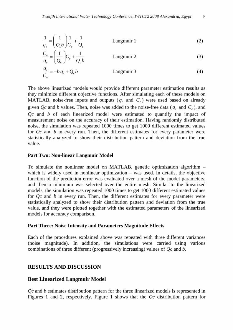
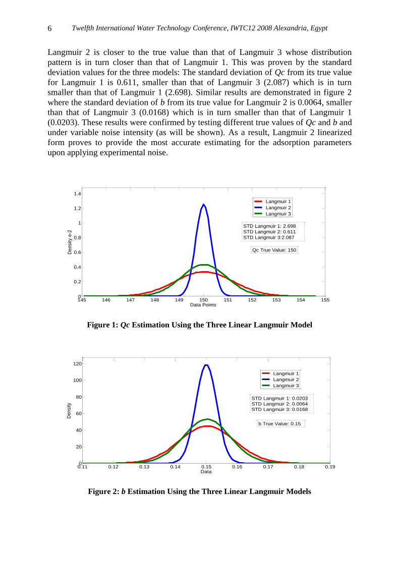
Qc and b estimates distribution pattern for the three linearized models is represented in
Figures 1 and 2, respectively. Figure 1 shows that the Qc distribution pattern for
Twelfth International Water Technology Conference, IWTC12 2008 Alexandria, Egypt
6
Langmuir 2 is closer to the true value than that of Langmuir 3 whose distribution
pattern is in turn closer than that of Langmuir 1. This was proven by the standard
deviation values for the three models: The standard deviation of Qc from its true value
for Langmuir 1 is 0.611, smaller than that of Langmuir 3 (2.087) which is in turn
smaller than that of Langmuir 1 (2.698). Similar results are demonstrated in figure 2
where the standard deviation of b from its true value for Langmuir 2 is 0.0064, smaller
than that of Langmuir 3 (0.0168) which is in turn smaller than that of Langmuir 1
(0.0203). These results were confirmed by testing different true values of Qc and b and
under variable noise intensity (as will be shown). As a result, Langmuir 2 linearized
form proves to provide the most accurate estimating for the adsorption parameters
upon applying experimental noise.
145 146 147 148 149 150 151 152 153 154 1550
0.2
0.4
0.6
0.8
1
1.2
1.4
Data Points
De
nsity e
-2
Langmuir 1
Langmuir 2
Langmuir 3
STD Langmuir 1: 2.698
STD Langmuir 2: 0.611
STD Langmuir 3:2.087
Qc True Value: 150
Figure 1: Qc Estimation Using the Three Linear Langmuir Model
0.11 0.12 0.13 0.14 0.15 0.16 0.17 0.18 0.190
20
40
60
80
100
120
Data
De
nsi
ty
Langmuir 1
Langmuir 2
Langmuir 3
STD Langmuir 1: 0.0203
STD Langmuir 2: 0.0064
STD Langmuir 3: 0.0168
b True Value: 0.15
Figure 2: b Estimation Using the Three Linear Langmuir Models
Twelfth International Water Technology Conference, IWTC12 2008 Alexandria, Egypt
7
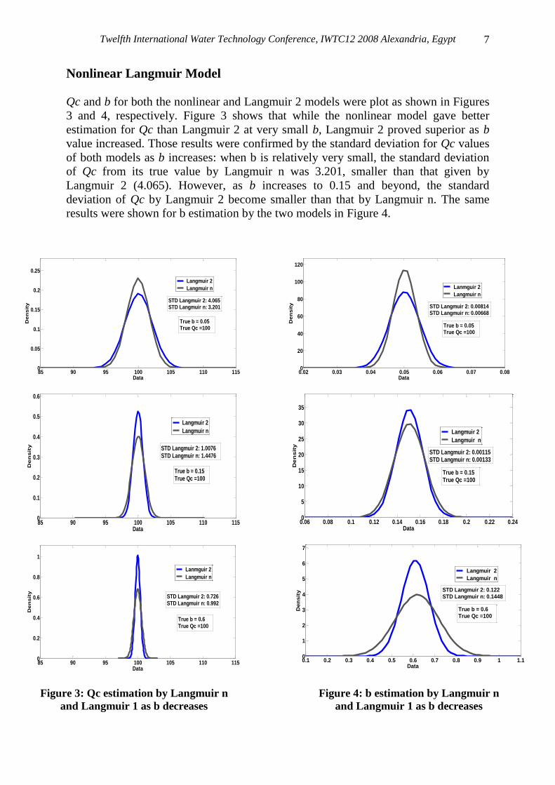
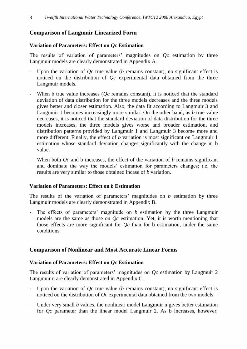
Nonlinear Langmuir Model
Qc and b for both the nonlinear and Langmuir 2 models were plot as shown in Figures
3 and 4, respectively. Figure 3 shows that while the nonlinear model gave better
estimation for Qc than Langmuir 2 at very small b, Langmuir 2 proved superior as b
value increased. Those results were confirmed by the standard deviation for Qc values
of both models as b increases: when b is relatively very small, the standard deviation
of Qc from its true value by Langmuir n was 3.201, smaller than that given by
Langmuir 2 (4.065). However, as b increases to 0.15 and beyond, the standard
deviation of Qc by Langmuir 2 become smaller than that by Langmuir n. The same
results were shown for b estimation by the two models in Figure 4.
85 90 95 100 105 110 1150
0.05
0.1
0.15
0.2
0.25
Data
De
ns
ity
Langmuir 2
Langmuir n
STD Langmuir 2: 4.065STD Langmuir n: 3.201
True b = 0.05True Qc =100
0.02 0.03 0.04 0.05 0.06 0.07 0.080
20
40
60
80
100
120
Data
De
ns
ity
Lanmguir 2
Langmuir n
True b = 0.05True Qc =100
STD Langmuir 2: 0.00814STD Langmuir n: 0.00668
85 90 95 100 105 110 1150
0.1
0.2
0.3
0.4
0.5
0.6
Data
De
ns
ity
Langmuir 2
Langmuir n
STD Langmuir 2: 1.0076STD Langmuir n: 1.4476
True b = 0.15True Qc =100
0.06 0.08 0.1 0.12 0.14 0.16 0.18 0.2 0.22 0.240
5
10
15
20
25
30
35
Data
De
ns
ity
Langmuir 2
Langmuir n
STD Langmuir 2: 0.00115STD Langmuir n: 0.00133
True b = 0.15True Qc =100
85 90 95 100 105 110 1150
0.2
0.4
0.6
0.8
1
Data
De
ns
ity
Lanmguir 2
Langmuir n
STD Langmuir 2: 0.726STD Langmuir n: 0.992
True b = 0.6True Qc =100
0.1 0.2 0.3 0.4 0.5 0.6 0.7 0.8 0.9 1 1.10
1
2
3
4
5
6
7
Data
De
ns
ity
Langmuir 2
Langmuir n
STD Langmuir 2: 0.122STD Langmuir n: 0.1448
True b = 0.6True Qc =100
Figure 3: Qc estimation by Langmuir n
and Langmuir 1 as b decreases
Figure 4: b estimation by Langmuir n
and Langmuir 1 as b decreases
Twelfth International Water Technology Conference, IWTC12 2008 Alexandria, Egypt
8
Comparison of Langmuir Linearized Form
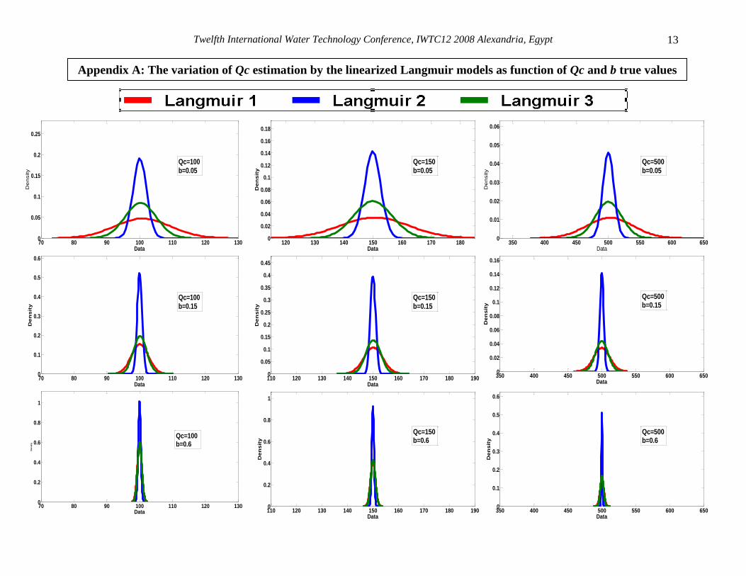
Variation of Parameters: Effect on Qc Estimation
The results of variation of parameters’ magnitudes on Qc estimation by three
Langmuir models are clearly demonstrated in Appendix A.
- Upon the variation of Qc true value (b remains constant), no significant effect is
noticed on the distribution of Qc experimental data obtained from the three
Langmuir models.
- When b true value increases (Qc remains constant), it is noticed that the standard
deviation of data distribution for the three models decreases and the three models
gives better and closer estimation. Also, the data fit according to Langmuir 3 and
Langmuir 1 becomes increasingly more similar. On the other hand, as b true value
decreases, it is noticed that the standard deviation of data distribution for the three
models increases, the three models gives worse and broader estimation, and
distribution patterns provided by Langmuir 1 and Langmuir 3 become more and
more different. Finally, the effect of b variation is most significant on Langmuir 1
estimation whose standard deviation changes significantly with the change in b
value.
- When both Qc and b increases, the effect of the variation of b remains significant
and dominate the way the models’ estimation for parameters changes; i.e. the
results are very similar to those obtained incase of b variation.
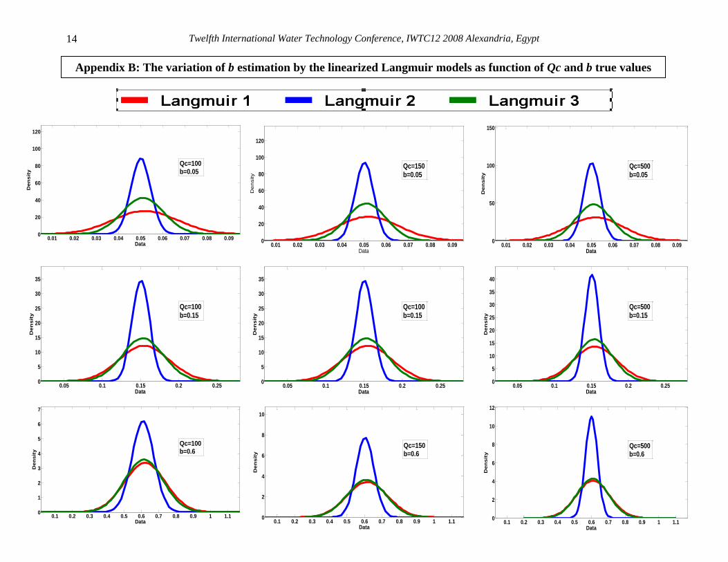
Variation of Parameters: Effect on b Estimation
The results of the variation of parameters’ magnitudes on b estimation by three
Langmuir models are clearly demonstrated in Appendix B.
- The effects of parameters’ magnitude on b estimation by the three Langmuir
models are the same as those on Qc estimation. Yet, it is worth mentioning that
those effects are more significant for Qc than for b estimation, under the same
conditions.
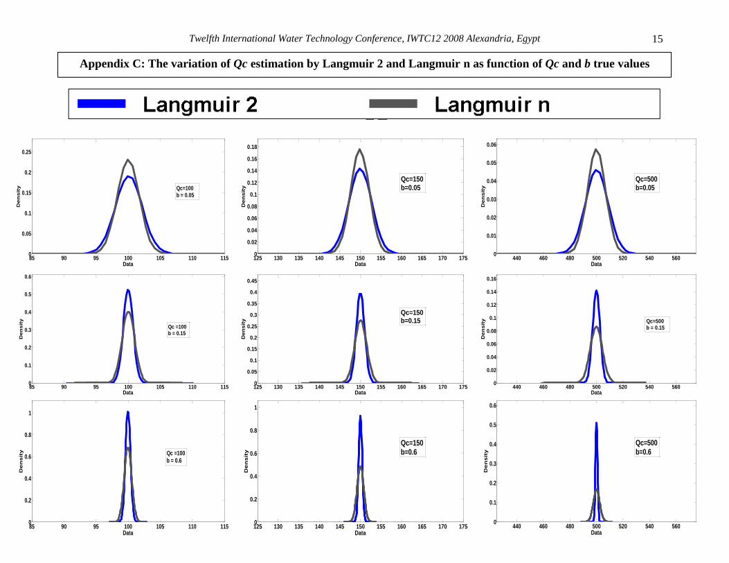
Comparison of Nonlinear and Most Accurate Linear Forms
Variation of Parameters: Effect on Qc Estimation
The results of variation of parameters’ magnitudes on Qc estimation by Langmuir 2
Langmuir n are clearly demonstrated in Appendix C.
- Upon the variation of Qc true value (b remains constant), no significant effect is
noticed on the distribution of Qc experimental data obtained from the two models.
- Under very small b values, the nonlinear model Langmuir n gives better estimation
for Qc parameter than the linear model Langmuir 2. As b increases, however,
Twelfth International Water Technology Conference, IWTC12 2008 Alexandria, Egypt
9
Langmuir 2 estimation improves and becomes even better than that of Langmuir n.
Also, as b true value increases, it is noticed that the standard deviation of data
distribution for the two models decreases and thus both models give better and
closer estimation.
- When both Qc and b increases, the effect of the variation of b remains significant
and dominate the way the models’ estimation for parameters changes; i.e. the
results are very similar to those obtained incase of b variation.
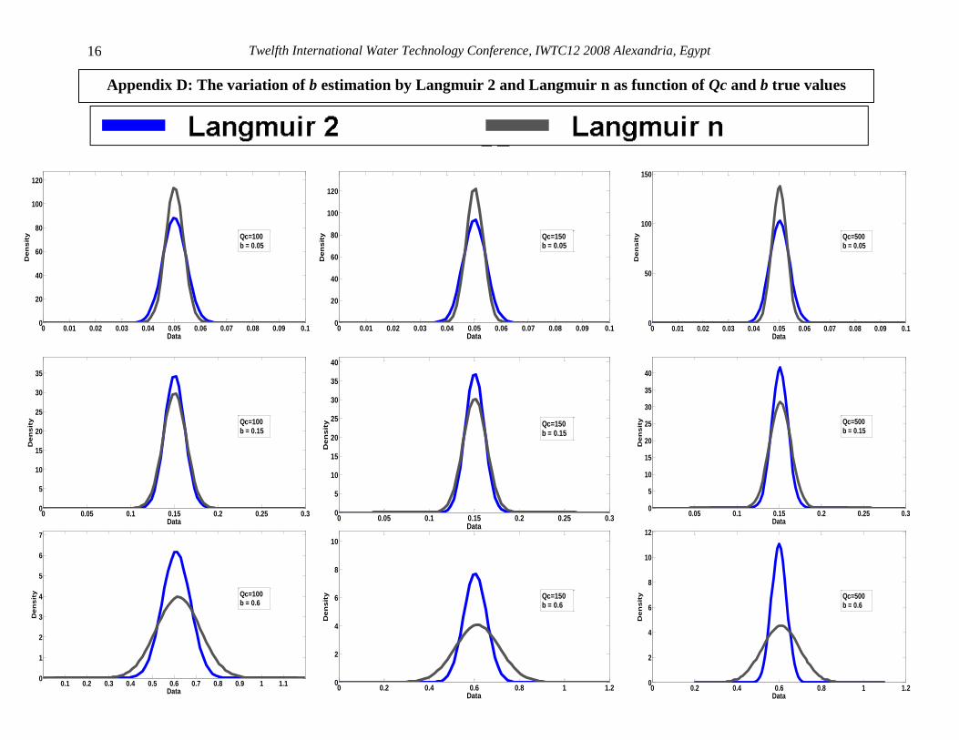
Variation of Parameters: Effect on b Estimation
The results of variation of parameters’ magnitudes on b estimation by Langmuir 2
Langmuir n are clearly demonstrated in Appendix D.
- Unlike all other cases, as Qc true value increases (b remains constant), the
estimation of b by both linear and nonlinear models slightly improves.
- Under very small b values, the nonlinear model Langmuir n gives better estimation
for b parameter than the linear model Langmuir 2. As b true value increases, its
estimation by Langmuir 2 improves and becomes even better than that of Langmuir
n. Also, as b true value increases, it is noticed that the standard deviation of data
distribution for the two models decreases and thus both models give better and
closer estimation. Yet, it is worth mentioning that the latter effect is more
significant for Qc than for b estimation, under the same conditions.
- When both Qc and b increases, the effect of the variation of b remains significant
and dominate the way the models’ estimation for parameters changes; i.e. the
results are very similar to those obtained incase of b variation.
Noise Variation Effect
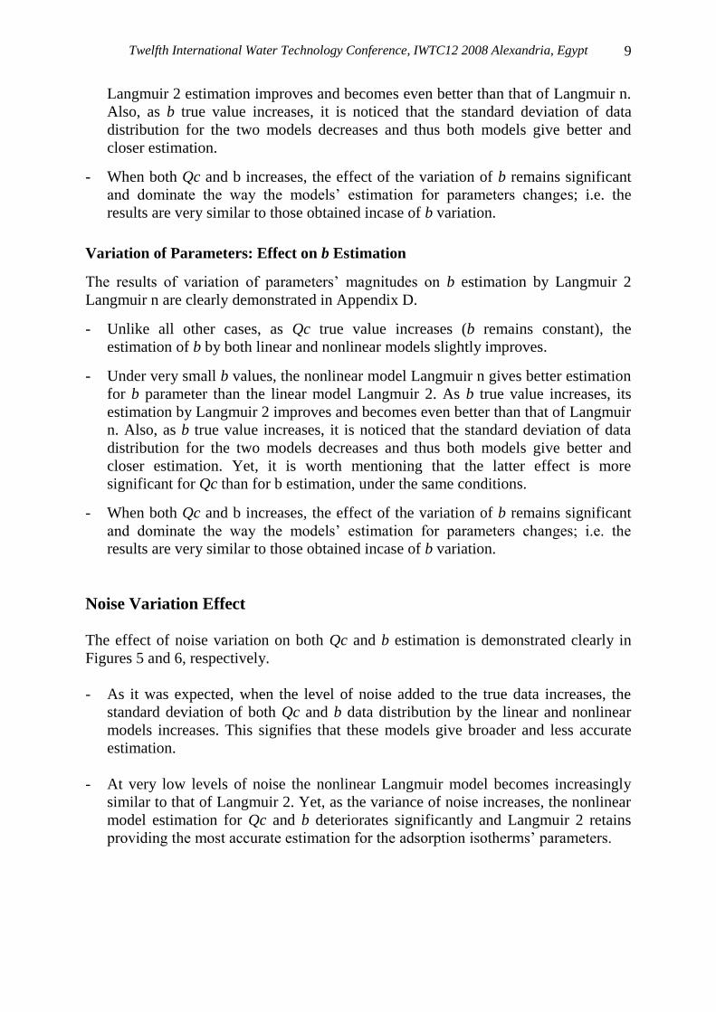
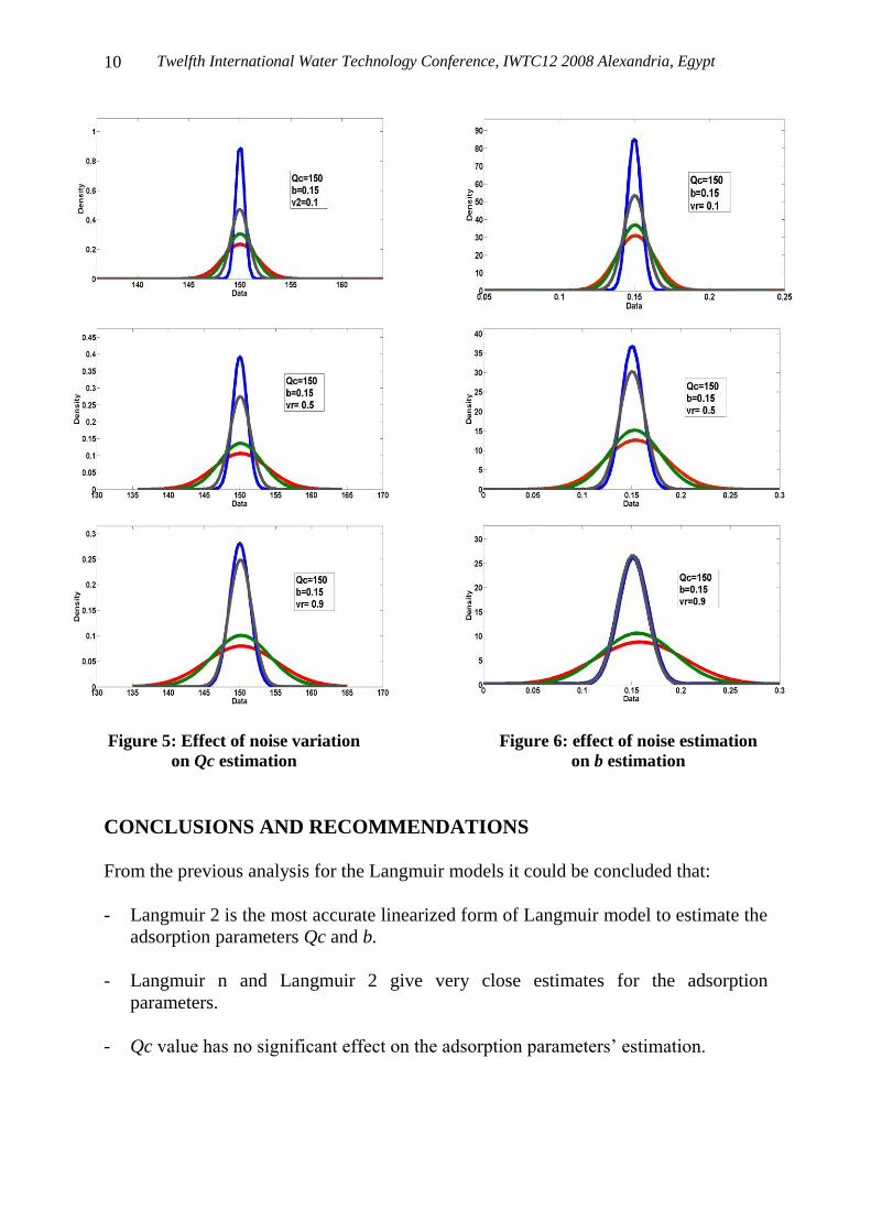
The effect of noise variation on both Qc and b estimation is demonstrated clearly in
Figures 5 and 6, respectively.
- As it was expected, when the level of noise added to the true data increases, the
standard deviation of both Qc and b data distribution by the linear and nonlinear
models increases. This signifies that these models give broader and less accurate
estimation.
- At very low levels of noise the nonlinear Langmuir model becomes increasingly
similar to that of Langmuir 2. Yet, as the variance of noise increases, the nonlinear
model estimation for Qc and b deteriorates significantly and Langmuir 2 retains
providing the most accurate estimation for the adsorption isotherms’ parameters.
Twelfth International Water Technology Conference, IWTC12 2008 Alexandria, Egypt
10
Figure 5: Effect of noise variation
on Qc estimation Figure 6: effect of noise estimation
on b estimation
CONCLUSIONS AND RECOMMENDATIONS
From the previous analysis for the Langmuir models it could be concluded that:
- Langmuir 2 is the most accurate linearized form of Langmuir model to estimate the
adsorption parameters Qc and b.
- Langmuir n and Langmuir 2 give very close estimates for the adsorption
parameters.
- Qc value has no significant effect on the adsorption parameters’ estimation.
Twelfth International Water Technology Conference, IWTC12 2008 Alexandria, Egypt
11
- As the affinity constant between the adsorbent and adsorbate magnitude increases:
the estimation of Qc and b by all models improves and Langmuir 2 proves
superior.
These results allow better understanding of the adsorption modeling by Langmuir.
Thus, depending on the experimental conditions specified, it would be easier to
determine which Langmuir form would give them most accurate adsorption
parameters and thus the most accurate modeling. In addition, the results prove to be of
significant practical value. From on side, now that it is known that the second
linearized form gives at least the accuracy than the original model, this linearized form
can be used with high level of confidence to get accurate estimations for the final
equilibrium solid phase concentration eq . On the other hand, the suggested Langmuir
2 provides a more accurate alternative for the linearizing the Langmuir model than
Langmuir 1 used by most industries.
Finally, after determining the best linear Langmuir model, comparing this model with
the original nonlinear form, and determining the effect of noise and parameters’
magnitude on the latter’s estimation accuracy, it is highly recommended to carry
similar analysis on other adsorption models (Freundlich, Redlich-Peterson, Sips…etc)
and compare their respective estimation accuracy with that of Langmuir n and
Langmuir 2. This would allow having a thorough knowledge about the parameters’
estimation accuracy of various adsorption models. Eventually, it would permit better
adsorption modeling and thus more accurate results in the various practical fields of
adsorption, especially water pollution.
ACKNOWLDGEMENTS
This publication was made possible by a grant from the Qatar National Research
Fund. Its contents are solely the responsibility of the authors and do not necessarily
represent the official views of the Qatar National Research Fund.
REFERENCES
[1] Hence, K.R., Water Environ. Res., 70, 1178 (1998).
[2] Ning, R.Y., Desalination, 143, 237 (2002).
[3] Alkan, M. and Dogan, M., J. Colloid Interface Sci, 243, 280 (2001).
[4] Dabaybeh, M. “Evaluation of Animal Solid Waster as a New Adsorbent”, M.S.
Thesis, Jordan University of Science and Technology (2001).
Twelfth International Water Technology Conference, IWTC12 2008 Alexandria, Egypt
12
[5] Otun, J. A., Oke, I. A., Olarinoye, N. O., Adie, D. B., and Okuofu, C. A.,
Journal of Applied Sciences. ANSInet, Asian Network for Scientific
Information, Faisalabad, Pakistan: 2006. 6: 11, 2368-2376. 26 ref.
[6] Pikaar, Ilje, Albert A. Koelmans and Paul C.M. van Noort, Sorption of organic
compounds to activated carbons. Evaluation of isotherm models, Chemosphere,
Volume 65, Issue 11, December 2006, Pages 2343-2351.
[7] Radhika, M., and Palanivelu, K., Adsorptive removal of chlorophenols from
aqueous solution by low cost adsorbent—Kinetics and isotherm analysis,
Journal of Hazardous Materials, Volume 138, Issue 1, 2 November 2006, Pages
116-124.
[8] Karahan, S., Yurdakoc, M., Seki, Y., and Yurdakoc, K., Removal of boron from
aqueous solution by clays and modified clays, Journal of Colloid and Interface
Science, Volume 293, Issue 1, 1 January 2006, Pages 36-42.
[9] Gormi, S., Seguin, J. L., Guerin, J., and Aguir, K., Erratum to “Adsorption–
desorption noise in gas sensors: Modelling using Langmuir and Wolkenstein
models for adsorption”, Sensors and Actuators B: Chemical, Volume 119, Issue
1, 24 November 2006, Page 351.
[10] Gritti, F., and Guiochon, G., Systematic errors in the measurement of
adsorption isotherms by frontal analysis: Impact of the choice of column hold-
up volume, range and density of the data points, Journal of Chromatography
A, Volume 1097, Issues 1-2, 2 December 2005, Pages 98-115.
[11] Gritti, F., and Guiochon, G., Accuracy and precision of adsorption isotherm
parameters measured by dynamic HPLC methods, Journal of Chromatography
A, Volume 1043, Issue 2, 23 July 2004, Pages 159-170.
[12] Joshi, M., A. Kremling, and Seidel-Morgenstern, A., Model based statistical
analysis of adsorption equilibrium data, Chemical Engineering Science,
Volume 61, Issue 23, December 2006, Pages 7805-7818.
Twelfth International Water Technology Conference, IWTC12 2008 Alexandria, Egypt
13
70 80 90 100 110 120 1300
0.05
0.1
0.15
0.2
0.25
Data
De
nsity
Qc=100b=0.05
120 130 140 150 160 170 1800
0.02
0.04
0.06
0.08
0.1
0.12
0.14
0.16
0.18
DataD
en
sit
y
Qc=150b=0.05
350 400 450 500 550 600 6500
0.01
0.02
0.03
0.04
0.05
0.06
Data
De
nsity
Qc=500b=0.05
70 80 90 100 110 120 1300
0.1
0.2
0.3
0.4
0.5
0.6
Data
De
ns
ity
Qc=100b=0.15
110 120 130 140 150 160 170 180 1900
0.05
0.1
0.15
0.2
0.25
0.3
0.35
0.4
0.45
Data
De
ns
ity
Qc=150b=0.15
350 400 450 500 550 600 6500
0.02
0.04
0.06
0.08
0.1
0.12
0.14
0.16
Data
De
ns
ity
Qc=500b=0.15
110 120 130 140 150 160 170 180 1900
0.2
0.4
0.6
0.8
1
Data
De
ns
ity
Qc=150b=0.6
350 400 450 500 550 600 6500
0.1
0.2
0.3
0.4
0.5
0.6
Data
De
ns
ity
Qc=500b=0.6
70 80 90 100 110 120 1300
0.2
0.4
0.6
0.8
1
Data
Den
sit
y
Qc=100b=0.6
Appendix A: The variation of Qc estimation by the linearized Langmuir models as function of Qc and b true values
Twelfth International Water Technology Conference, IWTC12 2008 Alexandria, Egypt
14
0.01 0.02 0.03 0.04 0.05 0.06 0.07 0.08 0.090
20
40
60
80
100
120
Data
De
ns
ity
Qc=100b=0.05
0.01 0.02 0.03 0.04 0.05 0.06 0.07 0.08 0.090
20
40
60
80
100
120
DataD
en
sity
Qc=150b=0.05
0.01 0.02 0.03 0.04 0.05 0.06 0.07 0.08 0.090
50
100
150
Data
De
ns
ity
Qc=500b=0.05
0.05 0.1 0.15 0.2 0.250
5
10
15
20
25
30
35
Data
De
ns
ity
Qc=100b=0.15
0.05 0.1 0.15 0.2 0.250
5
10
15
20
25
30
35
Data
De
ns
ity
Qc=100b=0.15
0.05 0.1 0.15 0.2 0.250
5
10
15
20
25
30
35
40
Data
De
ns
ity
Qc=500b=0.15
0.1 0.2 0.3 0.4 0.5 0.6 0.7 0.8 0.9 1 1.10
1
2
3
4
5
6
7
Data
De
ns
ity
Qc=100b=0.6
0.1 0.2 0.3 0.4 0.5 0.6 0.7 0.8 0.9 1 1.10
2
4
6
8
10
Data
De
ns
ity
Qc=150b=0.6
0.1 0.2 0.3 0.4 0.5 0.6 0.7 0.8 0.9 1 1.10
2
4
6
8
10
12
Data
De
ns
ity
Qc=500b=0.6
Appendix B: The variation of b estimation by the linearized Langmuir models as function of Qc and b true values
Twelfth International Water Technology Conference, IWTC12 2008 Alexandria, Egypt
15
85 90 95 100 105 110 1150
0.05
0.1
0.15
0.2
0.25
Data
De
ns
ity
Qc=100b = 0.05
125 130 135 140 145 150 155 160 165 170 1750
0.02
0.04
0.06
0.08
0.1
0.12
0.14
0.16
0.18
Data
De
ns
ity
Qc=150b=0.05
440 460 480 500 520 540 5600
0.01
0.02
0.03
0.04
0.05
0.06
Data
De
ns
ity
Qc=500b=0.05
85 90 95 100 105 110 1150
0.1
0.2
0.3
0.4
0.5
0.6
Data
De
ns
ity
Qc =100b = 0.15
125 130 135 140 145 150 155 160 165 170 1750
0.05
0.1
0.15
0.2
0.25
0.3
0.35
0.4
0.45
Data
De
ns
ity
Qc=150b=0.15
440 460 480 500 520 540 5600
0.02
0.04
0.06
0.08
0.1
0.12
0.14
0.16
Data
De
ns
ity
Qc=500b = 0.15
85 90 95 100 105 110 1150
0.2
0.4
0.6
0.8
1
Data
De
ns
ity
Qc =100b = 0.6
125 130 135 140 145 150 155 160 165 170 1750
0.2
0.4
0.6
0.8
1
Data
De
ns
ity
Qc=150b=0.6
440 460 480 500 520 540 5600
0.1
0.2
0.3
0.4
0.5
0.6
Data
De
ns
ity
Qc=500b=0.6
Appendix C: The variation of Qc estimation by Langmuir 2 and Langmuir n as function of Qc and b true values
Twelfth International Water Technology Conference, IWTC12 2008 Alexandria, Egypt
16
0 0.01 0.02 0.03 0.04 0.05 0.06 0.07 0.08 0.09 0.10
20
40
60
80
100
120
Data
De
ns
ity
Qc=100b = 0.05
0 0.01 0.02 0.03 0.04 0.05 0.06 0.07 0.08 0.09 0.10
20
40
60
80
100
120
Data
De
ns
ity
Qc=150b = 0.05
0 0.01 0.02 0.03 0.04 0.05 0.06 0.07 0.08 0.09 0.10
50
100
150
Data
De
ns
ity
Qc=500b = 0.05
0 0.05 0.1 0.15 0.2 0.25 0.30
5
10
15
20
25
30
35
Data
De
ns
ity
Qc=100b = 0.15
0 0.05 0.1 0.15 0.2 0.25 0.30
5
10
15
20
25
30
35
40
Data
De
ns
ity
Qc=150b = 0.15
0.05 0.1 0.15 0.2 0.25 0.30
5
10
15
20
25
30
35
40
Data
De
ns
ity
Qc=500b = 0.15
0.1 0.2 0.3 0.4 0.5 0.6 0.7 0.8 0.9 1 1.10
1
2
3
4
5
6
7
Data
De
ns
ity
Qc=100b = 0.6
0 0.2 0.4 0.6 0.8 1 1.20
2
4
6
8
10
Data
De
ns
ity
Qc=150b = 0.6
0 0.2 0.4 0.6 0.8 1 1.20
2
4
6
8
10
12
Data
De
ns
ity
Qc=500b = 0.6
Appendix D: The variation of b estimation by Langmuir 2 and Langmuir n as function of Qc and b true values

Twelfth International Water Technology Conference, IWTC12 2008 Alexandria, Egypt
17