Sensitivity of downward longwave surface radiation to moistureand cloud changes in a high-elevation region

Catherine M. Naud,1 Yonghua Chen,1 Imtiaz Rangwala,2,3 and James R. Miller 2

Received 22 February 2013; revised 6 June 2013; accepted 9 July 2013; published 11 September 2013.

[1] Several studies have suggested enhanced rates of warming in high-elevation regionssince the latter half of the twentieth century. One of the potential reasons why enhancedrates of warming might occur at high elevations is the nonlinear relationship betweendownward longwave radiation (DLR) and specific humidity (q). Using ground-basedobservations at a high-elevation site in southwestern Colorado and coincidentsatellite-borne cloud retrievals, the sensitivity of DLR to changes in q and cloud propertiesis examined and quantified using a neural network method. It is also used to explore howthe sensitivity of DLR to q (dDLR/dq) is affected by cloud properties. When binned byseason, dDLR/dq is maximum in winter and minimum in summer for both clear andcloudy skies. However, the cloudy-sky sensitivities are smaller, primarily because (1) forboth clear and cloudy skies dDLR/dq is proportional to 1/q, for q> 0.5 g kg�1, and (2) theseasonal values of q are on average larger in the cloudy-sky cases than in clear-sky cases.For a given value of q, dDLR/dq is slightly reduced in the presence of clouds and thisreduction increases as q increases. In addition, DLR is found to be more sensitive tochanges in cloud fraction when cloud fraction is large. In the limit of overcast skies, DLRsensitivity to optical thickness decreases as clouds become more opaque. These results arebased on only one high-elevation site, so the conclusions here need to be tested at otherhigh-elevation locations.

Citation: Naud, C.M., Y. Chen, I. Rangwala, and J. R.Miller (2013), Sensitivity of downward longwave surface radiationtomoisture and cloud changes in a high-elevation region, J. Geophys. Res. Atmos., 118, 10,072–10,081, doi:10.1002/jgrd.50644.

1. Introduction

[2] Mountain systems are critical to people and ecosys-tems, and they play a significant role as “water towers”within the terrestrial system. More than half of the globalrivers have their origins in mountains, and since midlatitudeto high-latitude rivers are often dominated by snowmelt run-off, it is important to understand how climate is changing inthese environments in response to increasing levels of atmo-spheric greenhouse gases [Christensen et al., 2007].[3] Since the latter half of the twentieth century, several

high-elevation regions may be experiencing a greater rateof warming than low-lying areas at the same latitude, andthe reason is still unclear [Rangwala and Miller, 2012 andreferences therein]. A number of positive feedbacks may bemore active in these cold and dry regions, and the water va-por feedback may be one of the most potent [Rangwalaand Miller, 2009; Rangwala, 2012]. One of the difficulties

in assessing these feedbacks is the sparsity of observationsin mountainous regions where radiation and cloud measure-ments are often missing. Several studies have already exam-ined the nonlinear relationship between humidity anddownward longwave radiation (DLR): the drier the atmo-sphere, the greater the impact of a small change in humidityon DLR [e.g., Ruckstuhl et al., 2007; Rangwala et al.,2010; Naud et al., 2012]. However, it is unclear how cloudsmay affect this sensitivity, i.e., if clouds are present, is the im-pact of a change in moisture on DLR reduced?[4] Using 6 years of ground-based observations of DLR

and specific humidity (q) collected at a high-elevation site(3719m altitude) in Colorado’s San Juan Mountains, and co-incident NASA Terra and Aqua Moderate resolutionImaging Spectroradiometer (MODIS) [Salomonson et al.,1989] cloud fraction and optical thickness retrievals, we eval-uate the impact of clouds on the DLR-q relationship. We notonly explore the change in sensitivity of DLR to changes inq, as a function of q, when clouds are present but also theimpact of changes in cloud fraction and optical thickness.[5] For this, we use a neural network (NN) method as an

alternative statistical method to traditional regression tech-niques; it has been widely used in environmental sciencesand water resources since the 1990s. A neural network is amapping model that relates one or several input variables toan output variable in a nonlinear way. In his review paper,Stephens [2005] recommends extending the classical feed-back diagnostics to investigate instantaneous sensitivities

1Department of Applied Physics and Applied Mathematics, ColumbiaUniversity, New York, New York, USA.

2Institute of Marine and Coastal Science, Rutgers, State University ofNew Jersey, New Brunswick, New Jersey, USA.

3WesternWater Assessment, PSDNOAAESRL, Boulder, Colorado, USA.

Corresponding author: C. M. Naud, Columbia University, 2880Broadway, New York, NY 10025, USA. (cn2140@columbia.edu)

©2013. American Geophysical Union. All Rights Reserved.2169-897X/13/10.1002/jgrd.50644

10,072

JOURNAL OF GEOPHYSICAL RESEARCH: ATMOSPHERES, VOL. 118, 10,072–10,081, doi:10.1002/jgrd.50644, 2013

instead of equilibrium estimates. These sensitivities con-stitute a step toward a more realistic representation andevaluation of feedback processes, particularly in theirtime evolution and their roles in governing cloud-radia-tion interactions. Stephens suggests that the Aires andRossow [2003] method is one way to obtain the instanta-neous sensitivities, that is, to apply a neural network ap-proach and examine the NN Jacobians.[6] The Jacobian matrix contains the first partial deriva-

tives of a given output variable with respect to a given inputvariable. This, by definition, is the sensitivity of the outputvariable to all input variables as inferred by the NN model.The neural network Jacobians can provide not only an esti-mate of the mean sensitivity between two variables but alsoan estimate of the distribution of the sensitivity. The advan-tage of this NN Jacobian is that it gives a direct statisticalevaluation of the multivariate and nonlinear sensitivities thatdepends on each configuration of input and output variables[Aires and Rossow, 2003]. Consequently, we examine notonly the NN outputs but also the Jacobian matrix within theneural network following the method of Aires and Rossow[2003]. Here, the input variables are specific humidity andeither cloud fraction or cloud optical thickness, and the out-put variable is DLR.

2. Data

[7] We use two different sets of data, one obtained from aground-based station and the other from a satellite. Both aredescribed below.

2.1. Senator Beck Study Plot

[8] The Center for Snow and Avalanche Studies (www.snowstudies.org) installed and manages four different mea-surement stations within the Senator Beck Basin in south-western Colorado. For our study, we choose one of thesesites, the Senator Beck Study Plot (37.9°N–107.725°W, alti-tude 3719m), because it is above tree line in an alpine tundraenvironment and exposed to strong winds that prevent coldair pooling issues as well as snow accumulation on the instru-ments. More detail on the site and instrumentation can befound in Painter et al. [2012]. Automated observations oftemperature, relative humidity, and downward longwaveand shortwave radiation (DLR and DSR), to only cite thoseused here, are performed every 5 s and provided as hourlyaverages, using the end of the hour as the reporting time(e.g., the 9A.M. observation includes all 5 s intervals be-tween 8A.M. and 9A.M.). The air temperature and relativehumidity are measured with a Campbell-Vaisala CS500-UHumitter® and the radiation with a Kipp and Zonen CG4180° field-of-view pyrgeometer for longwave and Kippand Zonen CM21 for shortwave. The instruments areleveled in situ, at the top of a tower; slight shifts may oc-cur after the operator gets off of the tower.[9] The radiometers were installed with the original manu-

facturer’s calibration and have gone through regular intervalsof calibration by AccuFlux per Annex A.3.1 of the ISO-9847Standard. Detailed information on the radiometers, includingtheir calibration and other history can be found at http://snowstudies.org/data/metadata/SBSP_metadata.pdf. The ra-diometers are sufficiently ventilated owing to strong windsat the study site. There have only been rare instances of snowaccumulation on the sensors (Landry, 2013, private commu-nication). The pyrgeometer includes a solar blind filter thatblocks all solar radiation. The solar radiation absorbed bythe silicon window covering the radiometer is conductedeffectively to facilitate very low heating effects even in fullsunlight and allows for accurate daytime measurementswithout the need for a shading disc. Both instruments areexpected to have an accuracy well within 2%, and as weexplore sensitivities, i.e., differences in fluxes, we do not ex-pect biases large enough to affect our conclusions.

(a) all observations

0 2 4 6 8 10 12100

150

200

250

300

350

DLR

(W

m-2)

(b) conservative cloud mask

0 2 4 6 8 10 12q (gkg-1)

100

150

200

250

300

350

DLR

(W

m-2)

y=219x overcast

y=152x clear

Figure 1. Daytime Senator Beck observations of down-ward longwave radiation (DLR) versus specific humidity(q), for clear (blue) and cloudy sky (red), using (a) allground-based observations and (b) ground-based observa-tions where the ground-based cloud mask and MODIS cloudfraction of exactly 0 and 100% (overcast) agree. The equa-tions represent a least square fit (solid lines).

Table 1. Daytime Seasonal Average of Sensitivity of DownwardLongwave Radiation DLR to Specific Humidity q (dDLR/dq) andSpecific Humidity (q) for Clear and Cloudy Sky, When BothCloud Masks Agree

Season

Clear Sky Cloudy Sky

q(g kg�1)

dDLR/dq(Wm�2(g kg�1)�1)

q(g kg�1)

dDLR/dq(Wm�2(g kg�1)�1)

Winter 1.3 36 2.8 18Spring 2.0 27 3.6 15Summer 3.9 17 7.7 8Autumn 3.2 19 4.9 11

10,073

NAUD ET AL.: DLR-Q SENSITIVITY TO CLOUDS IN MOUNTAINS

[10] For surface air pressure, we use measurements fromthe nearby Swamp Angel Study Plot (37.9°N–107.711°W;3371m) and estimate them for Senator Beck Study Plot usinga linear relationship of pressure with elevation. Although, airpressure changes exponentially with elevation along theatmospheric column, the assumption of a linear relationshipis valid for small elevation differences (here< 350m). Weuse the surface air pressure, along with relative humidityand temperature to calculate the specific humidity (q). Wealso estimated surface air pressure at the study site using ahypsometric equation. The difference in calculation of q fromthe two different pressure estimates is less than 6%.[11] The hourly DLR, DSR, and q data are available

from 2005 onward, but here we selected data over 6 yearsfrom the beginning of the collection. This gave a total of58,517 valid hourly observations of which 31,322 occurredduring daytime.

2.2. MODIS

[12] The moderate resolution imaging spectroradiometer(MODIS) is mounted on both NASA Terra and Aquaplatforms and observes the Earth with 36 channels at wave-lengths between 0.4 and 14μm since 1999 and 2002 respec-tively. The MODIS cloud retrievals are described in Platnicket al. [2003] and are archived in the MOD06 and MYD06files for Terra and Aqua platforms, respectively. Here we col-lect from both platforms the 5 min long granules that over-pass the Senator Beck station. This can occur 2–3 times aday, depending on the orbits. Only MODIS 5 km pixels thatcontain the ground site are used here. Cloud fractions (CF)are calculated from the 1 km cloud mask [Platnick et al.,2003; Ackerman et al., 2008], and thus vary between 0 and100% in 4% increments. Cloud optical thicknesses (τ) areavailable at 1 km, but here we only use the central pixel ina 5 × 5 km zone to match the cloud fraction resolution.These retrievals are only performed during the daytime

hours, because visible channels are used and only on pixelswith a near complete cloud fraction to avoid retrieval errorscaused by clear-sky contamination.[13] Uncertainties in the MODIS cloud mask are described

in Ackerman et al. [2008]. Clouds are missed when their op-tical thickness is less than 0.4 and also in polar regions atnight. However, daytime observations in these regions withbright surfaces were found to be mislabeled only 5% of thetime. We anticipate issues with the MODIS cloud fractionsin high-elevation regions to be largest in the winter whensnow is present, at night, and when thin cirrus are present.Consequently, some of the clear-sky points in our data setmay in fact contain clouds. For overcast scenes and opticalthicknesses greater than 0.4, the MODIS optical thicknessesare expected to be of good quality [e.g., Painemal andZuidema, 2011].[14] To relate cloud observations with the ground measure-

ments of q and DLR, we require the MODIS observing timeto be within the hour reported in the ground-based measure-ments. This reduces the daytime ground-based data set withcoincident cloud fraction to 3975 hourly observations. Thedata set is further reduced to 1491 hourly observations whenwe examine cloud optical thickness because it is only avail-able for mostly overcast 1 km pixels.

Senator Beck, daytime

0 2 4 6 8Average q per season (gkg-1)

0

10

20

30

40

Ave

rage

dD

LR/d

q pe

r se

ason

(W

m-2(g

kg-1)-1

)

* clear+ cloudy

Eq. (1a)Eq. (1b)dDLR/dq= 44.0/q+3.4

Figure 2. Seasonal average of dDLR/dq as a function ofaverage q for clear- (star) and cloudy- (cross) sky observa-tions as presented in Table 1. The dashed line represents alinear fit of both cloudy and clear-sky points as a functionof 1/q, while the solid line represents the first derivativeof equation (1a) and the dotted line the first derivative ofequation (1b).

(a) clear sky

0 2 4 6 8 10 12100

150

200

250

300

350

DLR

(W

m-2)

DLR

(W

m-2)

(b) cloudy sky

0 2 4 6 8 10 12q (gkg-1)

100

150

200

250

300

350

Figure 3. Downward longwave radiation (DLR) as a func-tion of specific humidity (q) for all (a) clear-sky and(b) cloudy-sky points processed by the neural network.The solid line shows the fit estimated by the neural net-work and the dashed line the fits given in equations(1a) for clear sky and (1b) for overcast sky.

10,074

NAUD ET AL.: DLR-Q SENSITIVITY TO CLOUDS IN MOUNTAINS

3. Methods

[15] In this section, we first describe how we delineateclear- and cloudy-sky conditions using a method based onground-based observations of incident solar radiation andthen describe the neural network technique.

3.1. Ground-Based Cloud Mask

[16] We use downward solar radiation measurements todetermine clear- and cloudy-sky conditions on a diurnal basisusing a strict criterion. For each month, if the daily meansolar radiation is one standard deviation above the monthlymean, we flag the whole diurnal period as a clear-sky case,and if the radiation is one standard deviation below themonthly mean, we flag it as a cloudy-sky case. All data pointswithin the one standard deviation are excluded from theanalysis, thereby reducing the ground-based daytime hourlydata pool to 10,424 hourly observations.[17] To assess the performance of this ground-based cloud

mask, we perform a comparison with the MODIS observa-tions. We require the measurements from the ground andsatellite to be coincident within half an hour and definethe MODIS cloud mask such as clear sky is for 0% cloudfraction and cloudy sky for 100% cloud fraction. We com-pare 931 daytime hourly observations and both platformsagree it was clear for 272 observations, agree it was cloudyfor 629 observations and disagree for 30 observations. Thisimplies a disagreement of only 3% between the two plat-forms during the daytime hours. Note that this disagreementincreases to 22% for the night time hourly observations.These results give great confidence in the ground-basedcloud mask for the daytime observations, and, therefore, onlydaytime observations are used for analysis in this study.

3.2. Neural Network

[18] The neural network (NN) approach is describedbriefly in this section. A much more detailed description, in-cluding an illustrative example, is given in Chen et al.[2006]. A neural network is a nonlinear mapping model that,given an input variable, provides an output quantity in anonlinear way. In this paper the output variable is DLR andthe input variables are specific humidity, cloud fraction,and cloud optical thickness.[19] A by-product of a neural network model is the

NN Jacobian matrix. This NN Jacobian matrix is equivalentto obtaining the first partial derivative of a given output var-iable with respect to a given input variable and will be a crit-ical component of our analysis in this paper. These Jacobianshave been used to add constraints in a radiative transfer

model [e.g., Aires et al., 1999] for variational assimilationapplications [Chevallier and Mahfouf, 2001] or to investigatesensitivities in a remote sensing algorithm [Aires et al.,2001]. In a different context, the NN Jacobians were inte-grated into a theoretical framework as a tool to study the in-stantaneous, multivariate, nonlinear sensitivities in climatefeedback processes [Aires and Rossow, 2003]. Chen et al.[2006] presented a test case that showed that NN estimatescould capture nonlinear relationships much better than thetraditional linear regression method. In this paper we usethe same NN model as Chen et al. [2006].[20] Initially, about half of the data are randomly selected

from the data set to train the neural network. The NN is opti-mized using the training data set, and the training process isstopped when the root mean square error between iterationsis small [Bishop, 1996]. The neural network structureobtained after this process is referred to as a trained neuralnetwork. Since there is some concern about overtraining inthe NN model, another portion of the original data set is usedto perform an independent validation of the trained neural

Table 2. Average Per NN Bin (From Low to High Sensitivity) of Clear Sky and Cloudy Skya

Clear Sky: Average Per Bin Cloudy Sky: Average Per Bin

NN Bins: Low toHigh dDLR/dq N

dDLR/dq(Wm�2 (g kg�1)�1)

DLR(Wm�2) q (g kg�1) T (°C) N

dDLR/dq(Wm�2 (g kg�1)�1)

DLR(Wm�2) q (g kg�1) T (°C)

1 552 11 (2) 267 6.7 10.8 634 5.4 (1) 301 6.9 4.72 1408 16 (2) 228 4.1 8.0 1530 8.4 (1) 301 6.5 3.93 826 24 (2) 207 2.7 3.3 1397 12.4 (1) 290 5.5 1.64 1909 32 (2) 171 1.6 �4.7 2168 18.2 (1) 254 2.5 �8.6

aN (number of points per bin), dDLR/dq (sensitivity of downward longwave radiation DLR to specific humidity q) with associated one standard devi-ation per bin in parenthesis, downward longwave radiation (DLR), specific humidity (q), and T is the surface air temperature. Each bin is of equal rangein dDLR/dq.

(a) clear sky

0 10 20 30 40

0.5

0.4

0.3

0.2

0.1

0.0

0.5

0.4

0.3

0.2

0.1

0.0

Fre

quen

cy o

f occ

urre

nce

(1)

(2)(3)

(4)

(b) cloudy sky

0 10 20 30 40dDLR/dq (Wm-2(gkg-1)-1)

Fre

quen

cy o

f occ

urre

nce

(1)

(2) (3)

(4)

Figure 4. Frequency of occurrence of dDLR/dq sorted intofour separate NN bins for (a) clear- and (b) cloudy-sky obser-vations. The frequency of occurrence is defined as the ratioof number of points per bin to the total number of points inthe data set. Each bin is of equal sensitivity range. SeeTable 2 for the average properties of each bin.

10,075

NAUD ET AL.: DLR-Q SENSITIVITY TO CLOUDS IN MOUNTAINS

network. If the errors between the NN predictions and thevalidation data set are small, we assume there is noovertraining in the NN model, and that the NN is providingthe correct output variables given the specified inputs. Onelimitation of the NN model is that it requires a large numberof data points, generally a few thousand, but we do haveenough for our analysis here.

[21] We apply the NN method to three sets of data: (1) thefull set with only ground observations during the daytimehours using the ground-based cloud mask (10,424 datapoints, section 4.1), (2) the subset for which MODIS cloudfractions are available (3975 data points, section 4.2), and(3) the subset of data for which MODIS cloud optical thick-nesses are available (1491 data points, section 4.3). In eachcase the output variable is DLR, and we are particularly inter-ested in the Jacobian matrix that provides the sensitivity ofDLR to changes in q and show how the sensitivities areaffected by clouds. We consider both bivariate (one inputvariable) and multivariate (two input variables) cases. Forthe bivariate case discussed in section 4.1, the input variableis q. For the multivariate cases, the input variables are qand cloud fraction (section 4.2), and q and cloud opticalthickness (section 4.3).

4. Results

[22] This section is divided into three parts. We first exam-ine the sensitivity of DLR to changes in q separately for clearand cloudy skies, regardless of cloud properties. In thesecond section we examine the effect of changes in cloudfraction on the DLR-q sensitivities. In the last section weinclude a discussion of the effect of changes in cloud opticalthickness (τ) on the sensitivities in overcast cases (cloudfractions of 100%). For all experiments, only daytime obser-vations are used to avoid inclusion of erroneous cloud detec-tions for both ground and satellite measurements.

Senator Beck, daytime

0 2 4 6 8

Average q per NN bin (gkg-1)

0

10

20

30

40

Ave

rage

dD

LR/d

q pe

r N

N b

in (

Wm

-2(g

kg-1)-1

)

* clear+ cloudy

Eq. (1a)Eq. (1b)dDLR/dq= 45.8/q+2.7

Figure 5. Average of dDLR/dq per NN bin as a function ofaverage q for clear- (star) and cloudy- (cross) sky conditionsas presented in Table 2. The dashed line is a linear fit in 1/q,the solid line is the first derivative of equation (1a), while thedotted line is the first derivative of equation (1b).

Figure 6. Frequency of occurrence of month per NN bin for (top) clear- and (bottom) cloudy-sky condi-tions (left to right) from low sensitivity (bin 1) to high sensitivity (bin 4). Each bin is of equal dDLR/dqrange. The frequency of occurrence is defined as the ratio of number of points per month to the total numberof points in the bin.

10,076

NAUD ET AL.: DLR-Q SENSITIVITY TO CLOUDS IN MOUNTAINS

4.1. DLR Sensitivity to Specific Humidity: Clear VersusCloudy Sky

[23] We first use all of the hourly observations measured atthe ground to examine the relationship between DLR and q,and we then apply the ground-based cloud mask to separateclear- from cloudy-sky cases. Figure 1a shows how the rela-tionship between DLR and q changes when clouds are pres-ent. Two distinct clusters can be seen, with DLR larger forthe cloudy-sky cluster as expected owing to the blackbodyeffect of the clouds on DLR. The clear-sky cluster exhibitsa longer tail toward the lower values of q, while the cloudy-sky cluster reaches further into the higher values of q.[24] Although two main clusters emerge as clear- and

cloudy-sky observations are delineated, there are many ob-servations that fall between these two main clusters. Thesepoints may be observations for which (1) the cloud mask iswrong, (2) the cloud fraction is small, or (3) the cloud opticalthickness is low. In order to correct for problems 1 and 2, weenforce a strict selection criterion that only retains observa-tions when both the ground-based and MODIS cloud masks(defined as clear sky for 0% cloud fraction and cloudy skyfor 100%) agree. For this subset, Figure 1b shows a betterseparation between clear- and overcast- (100% cloud frac-tion) sky observations, with overcast-sky DLR values beinglarger for a given q, and clear-sky values of q extending tolower values. We evaluate the relationship between DLRand q separately for clear- and overcast-sky conditions byapplying a regression fit to the log of DLR and q and obtain

DLR ¼ 152 q0:29 for clear sky (1a)

DLR ¼ 219 q0:19 for overcast sky (1b)

[25] A first order derivative of both fits indicates thatthe sensitivities at low values of q are slightly lower in over-cast conditions (e.g., for q = 2 g kg�1, dDLR/dq = 27 Wm�2

(g kg�1)�1 for clear sky and 23 Wm�2 (g kg�1)�1 forcloudy sky).[26] Table 1 shows the average seasonal dDLR/dq sensi-

tivities calculated from the slopes of the power law curves

shown in Figure 1b at mean seasonal q values associated withboth the clear- and overcast-sky cases. For both conditions,sensitivities are largest in the winter, and lowest in summer,but sensitivities are much lower for overcast sky. This isbecause the average seasonal q is larger when clouds arepresent, causing the sensitivities to decrease. By plottingthe relation between average sensitivity and average q asgiven in Table 1, we examine whether for a given q, the sen-sitivities change between clear- and cloudy-sky conditions.Figure 2 indicates the sensitivity is only slightly lower inthe presence of clouds (when overcast), although the two fitsobtained from equation (1) suggest this decrease in sensitiv-ity increases with increasing q. However, uncertainty inobservations and method prevent any definite conclusionas to the actual impact of clouds. A least square regressionassuming a linear relationship between the sensitivity and1/q also provides a reasonable fit to both clear- and cloudy-sky conditions, in between the first derivatives of equations(1a) and (1b).[27] We next use the NN to process all observations

(regardless of the value of the MODIS cloud fraction, as inFigure 1a) separately for clear- and cloudy-sky conditions(determined with the ground-based cloud mask). This allows

Table 3. Variable Correlation Matrix From NN Experiment WithDLR as a Function of q and Cloud Fraction (CF)

Variable/Variable DLR q CF

DLR 1.00 0.81 0.61q 0.81 1.00 0.30CF 0.61 0.30 1.00

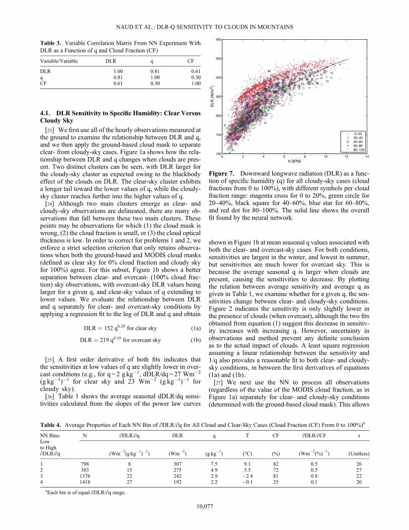
Figure 7. Downward longwave radiation (DLR) as a func-tion of specific humidity (q) for all cloudy-sky cases (cloudfractions from 0 to 100%), with different symbols per cloudfraction range: magenta cross for 0 to 20%, green circle for20–40%, black square for 40–60%, blue star for 60–80%,and red dot for 80–100%. The solid line shows the overallfit found by the neural network.

Table 4. Average Properties of Each NN Bin of ∂DLR/∂q for All Cloud and Clear-Sky Cases (Cloud Fraction (CF) From 0 to 100%)a

NN Bins:Lowto High∂DLR/∂q

N ∂DLR/∂q DLR q T CF ∂DLR/∂CF τ

(Wm�2(g kg�1)�1) (Wm�2) (g kg�1) (°C) (%) (Wm�2(%)�1) (Unitless)

1 798 8 307 7.5 9.1 82 0.5 262 383 15 275 4.9 5.5 72 0.5 273 1376 22 242 2.9 �2.4 81 0.8 224 1418 27 192 2.2 �0.1 25 0.1 20

aEach bin is of equal ∂DLR/∂q range.

10,077

NAUD ET AL.: DLR-Q SENSITIVITY TO CLOUDS IN MOUNTAINS

us to verify if the results from the NN method are consistentwith the least square regression method used above, and fur-ther helps in their interpretation. Figure 3a shows a scatterplot of DLR versus q for all points used in the neural networkfor clear sky only, while Figure 3b shows the cloudy-skycase. The solid line represents a fit automatically generatedby the NN, while the dashed lines show the fits given byequations (1a) and (1b). For clear-sky conditions, theNN method gives a fit very similar to the one found forthe restricted data set in Figure 1b. For cloudy-sky cases,the correspondence between equation (1b) and the NN fit isfairly good for q< 4 g kg�1 but there is more deviation forlarger values of q. Part of this bias would arise from thefact that for the NN fit all cloudy points are included, whileequation (1b) is only for strictly overcast cases. This suggeststhe inclusion of cloud fractions less than 100% has a largerimpact on the DLR-q relationship for larger values of q.In addition, the number of observations decreases rapidlywith q for q> 4 g kg�1, which may also affect the qualityof both fits.[28] The NN results are then binned according to specified

criteria, e.g., month, sensitivity, cloud fraction, q, and cloudoptical thickness. We sort the results by sensitivity into fourbins with equal sensitivity range for each bin. If one desireshigher resolution of the sensitivities, then more bins can bespecified. Since the ranges of sensitivities in each of the fourbins are equal, there is no expectation that each bin will con-tain the same number of observations, and Table 2 shows thatto be the case. Table 2 also includes the mean quantities foreach bin and the standard deviation of the sensitivities per

bin. Figure 4 shows the frequency of occurrence of theDLR-q sensitivities sorted into these four separate bins forboth clear- and cloudy-sky conditions. For both clear- andcloudy-sky conditions, the lowest sensitivity bin is the leastpopulated while the highest sensitivity bin is the most popu-lated. For all four sensitivity bins, cloudy-sky conditionsexhibit lower sensitivities than clear-sky conditions. Whenexploring the relationship between the average sensitivityand average q per bin (Table 2), for both clear- and cloudy-sky conditions, Figure 5 shows that we obtain a linear fit in1/q that is very close to the seasonal relationship shown inFigure 2. However, there is more scatter in the cloudy-skypoints (cf. Figure 3b), and it becomes difficult to reconcilethe overcast sky fit of equation (1b) (dotted line) with thecloudy-sky points in Figure 5 at the lower sensitivity—larger q end.[29] We next examine the temporal distribution of each of

the four bins in Figure 4 by separating the sensitivities bymonth for both clear- and cloudy-sky conditions. Figure 6reveals that the lowest sensitivity bin (bin 1) contains mostlysummer months, for both clear- and cloudy-sky conditions,although for cloudy conditions, late spring and early fallare also represented. The second bin includes, in both cases,late spring, summer, and early fall. For the third bin, the dis-tribution is slightly different between clear- and cloudy-skyconditions, with most months represented for both, butwith a peak in late spring for clear-sky cases and a peak insummer for cloudy-sky cases. Finally, the highest sensitivitybin (bin 4) occurs in winter and early spring for both clear-and cloudy-sky conditions. Compared with the sensitivities

Figure 8. Frequency of occurrence of (a) ∂DLR/∂q and (b)∂DLR/∂CF sorted into four NN bins where CF is cloud frac-tion. The frequency of occurrence is defined as the ratio ofnumber of points per bin to the total number of points inthe data set. Each bin is of equal sensitivity range. SeeTable 4 for average properties of each bin in Figure 8a andTable 5 for Figure 8b.

Table 5. Same as Table 4 but for Bins of Equal ∂DLR/∂CF Range

NN Bins:Lowto High∂DLR/∂CF

N ∂DLR/∂CF DLR q T CF ∂DLR/∂q τ

(Wm�2(%)�1) (Wm�2) (g kg�1) (°C) (%) (Wm�2(g kg�1)�1) (Unitless)

1 1119 �0.2 187 2.2 1.6 4 25 NA2 662 0.3 264 5.9 8.2 45 16 273 1355 0.7 278 5.0 3.3 92 16 244 839 1.1 232 2.1 �7.0 97 24 22

Figure 9. Downward longwave radiation (DLR) as a func-tion of specific humidity (q) for cloudy-sky conditions, withdifferent colors for different cloud optical thicknesses τ: 0–20(blue), 20–40 (red), 40–60 (orange), 60–80 (green), and 80–100 (black).

10,078

NAUD ET AL.: DLR-Q SENSITIVITY TO CLOUDS IN MOUNTAINS

given in Table 1 where seasons are intentionally sepa-rated, the lowest and highest sensitivity bins obtainedwith the NN strongly resemble the summer and wintersensitivities, respectively.[30] Using both the NN and a direct method, we find that

the sensitivity of DLR to changes in q is similar whetherclouds are present or not, albeit with a slight reduction incloudy-sky DLR-q sensitivities for a given q. In this section,our focus has been on clear- and cloudy-sky conditionsregardless of cloud properties; we next investigate the impactof changing cloud fraction.

4.2. DLR Sensitivity to Specific Humidity andCloud Fraction

[31] We now use the neural network to investigate sensitiv-ities of DLR to both changes in q and cloud fraction. Thisexperiment is conducted on the subset for which MODIScloud fractions are available (3975 data points). The NN var-iable correlation matrix (Table 3) indicates a stronger correla-tion between DLR and q than between DLR and cloudfraction. Also, it shows that the correlation between q andcloud fraction is low.[32] Figure 7 shows the relationship between DLR and q

for all points with cloud fractions between 0 (clear sky) and100% (overcast). It also shows how this relationship changeswith cloud fraction and how most observations with a cloudfraction less than 80% fall onto the clear-sky cluster whilefractions greater than 80% tend to follow the overcast cluster(see Figure 1b). The all-points NN fit tends to be closer to theclear-sky/low cloud fraction cluster than the overcast cluster.[33] For the two-variable experiment with changes in q and

CF, the NN output is first partitioned into four distinct bins ofequal ∂DLR/∂q range for all observations including thosewith intermediate cloud fraction, clear, and overcast skies.Table 4 gives the average properties for each bin, andFigure 8a shows the frequency of occurrence of the ∂DLR/∂q bins. The distribution of sensitivities differs slightly frompurely clear- or overcast-sky cases (see Figure 4). The sensi-tivities in each bin lie between those in the clear- and cloudy-sky bins, and we find that they align with the 1/q fit in

Figure 5 (not shown). Focusing on the two highest sensitivitybins, 3 and 4, we find that their properties are very different(Table 4). For bin 3, the cloud fractions are large (around80% on average), while for bin 4, the cloud fractions arelow (around 25%). Also, the sensitivity of DLR to changesin cloud fraction in bin 3 is much larger than in bin 4.Finally, bin 3 is colder with slightly larger mean specifichumidity than bin 4. Thus, for similar DLR-q sensitivities(22 versus 27 Wm�2(g kg�1)�1 for bins 3 and 4, respec-tively), and fairly close values of q (2.9 versus 2.2 g kg�1),the bin with high cloud fractions exhibits sensitivities ofDLR to q of the same order as the bin with the low cloudfractions. This suggests that cloud fraction has a minorimpact on the sensitivity of DLR to q, at least for q between2 and 3 g kg�1.[34] We now examine the same outputs but this time

partitioned into four bins of equal sensitivity to cloud frac-tion. This differs from the discussion in the previous para-graph because the binning is now performed according tothe sensitivities of DLR to changes in cloud fraction ratherthan to changes in q. Table 5 summarizes the average proper-ties of each bin, and Figure 8b shows the frequency of occur-rence of each bin. The distribution displays fewer highsensitivity points as compared to other distributions that havebeen shown. Table 5 shows that cloud fraction is positivelycorrelated with DLR-CF sensitivities, i.e., higher values ofcloud fraction associated with higher values of DLR-CFsensitivities. The lowest and highest DLR-CF sensitivitybins also correspond to cases with low specific humidity(2.2 versus 2.1 g kg�1) and high DLR-q sensitivities (25

Table 6. Variable Correlation Matrix From NN Experiment WithDLR as a Function of q and Cloud Optical Thickness τ

Variable/Variable DLR q τ

DLR 1.00 0.85 0.21q 0.85 1.00 0.10τ 0.21 0.10 1.00

Table 7. Same as Table 4 for Data Set With Overcast Clouds and Cloud Optical Thickness (τ) Retrievalsa

NN Bins:Lowto High∂DLR/∂q

N ∂DLR/∂q DLR q T ∂DLR/∂τ τ

(Wm�2(g kg�1)�1) (Wm�2) (g kg�1) (°C) (Wm�2) (Unitless)

1 379 8 320 7.8 7.9 0.4 292 210 13 292 5.0 2.3 0.5 283 290 17 271 3.6 �2.3 0.5 284 612 22 243 2.3 �7.5 0.7 19

aEach bin is of equal ∂DLR/∂q range.

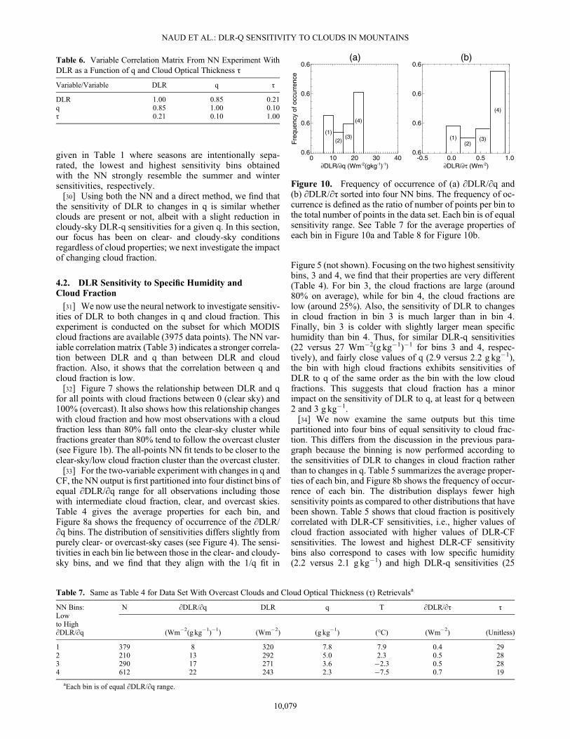
Figure 10. Frequency of occurrence of (a) ∂DLR/∂q and(b) ∂DLR/∂τ sorted into four NN bins. The frequency of oc-currence is defined as the ratio of number of points per bin tothe total number of points in the data set. Each bin is of equalsensitivity range. See Table 7 for the average properties ofeach bin in Figure 10a and Table 8 for Figure 10b.

10,079

NAUD ET AL.: DLR-Q SENSITIVITY TO CLOUDS IN MOUNTAINS

versus 24 Wm�2(g kg�1)�1). This means that, at low valuesof q (~2 g kg�1) and high values of DLR-q sensitivities, whencloud fractions are low, DLR is marginally sensitive tochanges in cloud fraction but when the cloud fraction is large,DLR is very sensitive to changes in cloud fraction. Thissuggests that at high cloud fraction, the ∂DLR/∂CF sensi-tivity does not saturate in the low q range. Next, we in-vestigate the impact of cloud optical thickness duringovercast conditions.

4.3. DLR Sensitivity to Specific Humidity and CloudOptical Thickness

[35] As explained earlier, MODIS optical thickness re-trievals are only performed during the daytime for pixels thatare mostly overcast. Therefore, we can study the impactof changes in optical thickness without much interferencefrom changes in cloud fraction. This means the subset ofpoints used will be smaller than those described in section4.2 (i.e., 1491 instead of 3975 data points). Figure 9 showsthe relationship between DLR and q in overcast situationsas a function of cloud optical thickness (color coded). Thepoints are transitioning from the cloudy to clear-sky clusteras clouds become more transparent (τ< 20). This is similarto the behavior we observed when cloud fraction decreased.Table 6 shows the variable matrix for this NN experiment,with DLR and q highly correlated while DLR and cloudoptical thickness are weakly correlated.[36] For this subset of points (overcast with an optical

thickness retrieval available), we again partition the outputdata points into four equal range bins based on the valuesof ∂DLR/∂q. The lowest DLR-q sensitivity bin exhibits thehighest values of cloud optical thickness, while the highestsensitivity bin exhibits the lowest values of cloud opticalthickness (Table 7). The neural network yields a bimodal dis-tribution of sensitivities of DLR to q (Figure 10a), with themaximum occurrence for the lowest and highest sensitivitybins. In fact, Table 7 shows little change in optical thicknessfor bins one through three. This suggests that thicker cloudsreduce the impact of q on DLR, while as clouds become moretransparent, the impact of q on DLR increases.[37] Then we partition the data points into four bins of

equal ∂DLR/∂τ range. The average properties of each binare given in Table 8, and Figure 10b shows the distributionof sensitivity of DLR to cloud optical thickness in the fourbins. There are two main modes of DLR sensitivities tochanges in τ, one highly populated for the highest sensitivi-ties and the second most populated mode is for the lowestsensitivity. We find that low DLR-τ sensitivities correspondto cases with high optical thickness and relatively large q(Table 8). Considering bins 1 to 3 where DLR, q, and

∂DLR/∂q are fairly similar, the DLR-τ sensitivity increasesas the optical thickness decreases.[38] These results suggest that in overcast situations, as

optical thickness increases, sensitivity of DLR to τ decreases.Furthermore, for mean τ ≥ 20 (bins 1–3), ∂DLR/∂q, and qremain more or less constant which suggests a saturationeffect whereby the impact of changes in τ has less and lesseffect on DLR-q sensitivities once τ is above a certain value.However, ∂DLR/∂τ and ∂DLR/∂q are largest for semitrans-parent clouds (mean τ= 8).

5. Conclusions

[39] Using ground-based observations of DLR and q at onehigh-elevation location in southwestern Colorado, we inves-tigate the relationship between these two variables, in cloud-free and cloudy conditions. Both a simple regression and aneural network method suggest that clouds not only increaseDLR for a given q, they also slightly reduce the sensitivity ofDLR to q, and this reduction increases with increasing q.Despite uncertainties in the measurements themselves andin the method that may affect the significance of these results,this reduction is consistent with previous work by Ruckstuhlet al. [2007]. They examined the sensitivity of DLR to q forclear- and all-sky conditions and found a slightly lower sen-sitivity in all-sky conditions.[40] Overall, the sensitivity of DLR to changes in cloud

fraction increases with cloud fraction. When the sky isovercast, DLR is sensitive to changes in optical thickness.However, as clouds become optically thicker, DLR reachessaturation and additional changes in DLR with cloud opticalthickness are small. The sensitivity of DLR to changes in q islargest at low values of q, and in these conditions, cloudfraction changes have a minor impact on this sensitivity.However, for overcast clouds in fairly humid conditions,increases in optical thickness tend to decrease the DLR-q sensitivity.[41] For each neural network experiment, we find that the

highest sensitivities to changes in q are the following:[42] 1. 32 Wm�2(g kg�1)�1 for 0< q< 2 g kg�1

(clear sky);[43] 2. 18 Wm�2(g kg�1)�1 for 1.5< q< 3.5 g kg�1

(cloudy sky, 100% cloud fraction);[44] 3. 27 Wm�2(g kg�1)�1 for 0< q< 4 g kg�1 (all cloud

fractions from 0 to 100% included); and[45] 4. 22 Wm�2(g kg�1)�1 for 0< q< 4 g kg�1 (cloudy

sky, 100% fraction, optical thickness retrieved)which means for a change in q of 2 g kg�1, DLR changes byup to 65Wm�2, 36Wm�2, 54Wm�2, and 44Wm�2, respec-tively. The differences among these sensitivities are causedin part by different ranges of q within the highest sensitivity

Table 8. Same as Table 7 but for Bins of Equal ∂DLR/∂τ Range

NN Bins:Lowto High∂DLR/∂τ

N ∂DLR/∂τ DLR q T τ ∂DLR/∂q

(Wm�2) (Wm�2) (g kg�1) (°C) (Unitless) (Wm�2(g kg�1)�1)

1 269 �0.0 293 5.1 -1.0 75 132 151 0.3 294 5.3 0.1 31 143 245 0.6 290 5.1 0.3 20 144 826 0.8 261 3.7 �1.9 8 18

10,080

NAUD ET AL.: DLR-Q SENSITIVITY TO CLOUDS IN MOUNTAINS

bins. Potentially, the nighttime observations (not consideredhere) during winter or spring will have even drier and colderconditions, which will lead to realizations of even highermagnitudes of DLR-q sensitivities. Preliminary tests confirmthis hypothesis, but issues with the cloud mask need to beresolved before any definite conclusion can be reached. Wealso note here that these changes in DLR are likely to beupper bounds on the response to changes in q because in-creases in temperature cause DLR to increase, and we havenot considered the impact of changes in temperature whichtend to be positively correlated with changes in q.[46] Quantifying the influence of cloud properties on DLR,

we find a DLR change of 0.8 Wm�2 per unit of optical thick-ness when optical thickness is between 0 and 20, and a DLRchange of 1.1 Wm�2(%)�1 for cloud fraction between 80 and100%. These entail a maximum change in DLR of 16 Wm�2

for a 20 unit change in optical thickness, and a DLR changeof 22 Wm�2 for a 20% change in cloud fraction. In general,we find the impact on DLR from a change in q, for the rangeof q available at this elevation, to be greater than that from achange in either cloud optical thickness or cloud fraction.Although these numbers are only indicative of what the realcloud effect might be, these results are qualitatively sound,as errors in the MODIS retrievals will mostly affect nighttimeobservations which are not used here. In addition, opticallythin clouds, which are also a source of errors for MODIS re-trievals, are not found to have a large impact. Furthermore,ground measurement uncertainties are small and suffer fromno systematic bias, and are further reduced by using multipleyears and a large sample.[47] Overall, our experiments suggest the presence of

clouds has a very limited influence on the sensitivity ofDLR to q in the low q range (<5 g kg�1). However, at highervalues of q, clouds tend to reduce this sensitivity. In thecontext of a future warming at high elevations, which maybe accompanied by increases in the atmospheric moisture,winter and early spring may see a significant increase inDLR and possibly accelerated warming that could be par-tially offset by a change in cloud properties. These resultsare obtained using only one high-elevation site during day-time, but include a large sample size that should reducethe impact of measurement uncertainties and interannual var-iability (which was found to cause an uncertainty of nogreater than 10% in the exponents of equation (1)). The lowvalues of the standard deviations of the seasonal sensitivitiesprovide additional evidence that the errors in sensitivities aresmall. Nevertheless, further work is needed to include night-time observations and compare our results with other high-elevation locations.

[48] Acknowledgments. The Senator Beck Basin observations areprovided by the Center for Snow and Avalanche Studies (http://www.snowstudies.org/). The MODIS cloud product (MOD06/MYD06) files areprovided by the Level 1 and Atmospheric Archive Distribution System atthe NASA Goddard Space Flight Center. We thank Filipe Aires for helpfuldiscussions of the neural net analysis and Chris Landry for information andclarification related to instrumentation at the Senator Beck study site. We

also thank three anonymous reviewers for significantly improving this man-uscript. This work is funded by the NSF grants 1064281 and 1064326.

ReferencesAckerman, S. A., R. E. Holz, R. Frey, E. W. Eloranta, B. C. Maddux, andM. McGill (2008), Cloud detection with MODIS. Part II: Validation,J. Atmos. Oceanic Technol., 25, 1073–1086.

Aires, F., and W. B. Rossow (2003), Inferring instantaneous, multivariateand nonlinear sensitivities for the analysis of feedback processes in a dy-namical system: The Lorenz model case study, Quart. J. Roy. Meteorol.Soc., 129, 239–275.

Aires, F., M. Schmitt, N. Scott, and A. Chedin (1999), The weight smooth-ing regularisation for MLP for resolving the input contribution’s errorsin functional interpolations, IEEE Trans. Neural Networks, 10,1502–1510.

Aires, F., C. Prigent, W. B. Rossow, and M. Rothstein (2001), A new neuralnetwork approach including first-guess for retrieval of atmospheric watervapor, cloud liquid water path, surface temperature and emissivities overland from satellite microwave observations, J. Geophys. Res., 106,14,887–14,907.

Bishop, C. M. (1996), Neural Networks for Pattern Recognition, pp. 482,Oxford University Press, Oxford.

Chen, Y., F. Aires, J. A. Francis, and J. R. Miller (2006), Observed relation-ships between Arctic longwave cloud forcing and cloud parameters using aneural network, J. Climate, 19, 4087–4104.

Chevallier, F., and J. F. Mahfouf (2001), Evaluation of the Jacobians ofinfrared radiation models for variational data assimilation, J. Appl.Meteorol., 40, 1445–1461.

Christensen, J. H., B. Hewitson, A. Busuioc, A. Chen, X. Gao, R. Held,R. Jones, R. K. Kolli, W. Kwon, and R. Laprise (2007), Regional climateprojections, Climate Change, 2007: The Physical Science Basis.Contribution of Working group I to the Fourth Assessment Report of theIntergovernmental Panel on Climate Change, University Press,Cambridge, Chapter 11 (Box 11.3), 847-940.

Naud, C. M., J. R. Miller, and C. Landry (2012), Using satellites to investi-gate the sensitivity of longwave downward radiation to water vapor at highelevations, J. Geophys. Res., 117, D05101, doi:10.1029/2011JD016917.

Painemal, D., and P. Zuidema (2011), Assessment of MODIS cloud effec-tive radius and optical thickness retrievals over the Southeast Pacificwith VOCALS-Rex in situ, J. Geophys. Res., 116, D24206, doi:10.1029/2011JD016155.

Painter, T. J., S. McKensie Skiles, J. S. Deems, A. C. Bryant, andC. C. Landry (2012), Dust radiative forcing in snow of the UpperColorado River Basin: 1. A 6 year record of energy balance, radiation,and dust concentrations, Water Resour. Res., 48, W07521, doi:10.1029/2012WR011985.

Platnick, S., M. D. King, S. A. Ackerman, W. P. Menzel, B. A. Baum,J. C. Riédi, and R. A. Frey (2003), The MODIS cloud products: Algorithmsand examples from Terra, IEEE Trans. Geosci. Remote Sens., 41, 459–472.

Rangwala, I. (2012), Amplified water vapor feedback at high altitudes duringwinter, Int. J. Climatol., doi:10.1002/joc.3477.

Rangwala, I., and J. R. Miller (2009), Warming in the Tibetan Plateau:Possible influences of the changes in surface water vapor, Geophys. Res.Lett., 36, L06703, doi:10.1029/2009GL037245.

Rangwala, I., and J. R. Miller (2012), Climate change in mountains: Areview of elevation-dependent warming and its possible causes, Clim.Change, doi:10.1007/s10584-012-0419-3.

Rangwala, I., J. Miller, G. Russell, andM. Xu (2010), Using a global climatemodel to evaluate the influences of water vapor, snow cover and atmo-spheric aerosol on warming in the Tibetan Plateau during the twenty-firstcentury, Climate Dynam., 34(6), 859–872.

Ruckstuhl, C., R. Philipona, J. Morland, and A. Ohmura (2007), Observedrelationship between surface specific humidity, integrated water vapor,and longwave downward radiation at different altitudes, J. Geophys.Res., 112, L19809, doi:10.1029/2005GL023624.

Salomonson, V. V., W. L. Barnes, P. W. Maymon, H. E. Montgomery, andH. Ostrow (1989), MODIS: Advanced facility instrument for studies of theEarth as a system, IEEE Trans. Geosci. Remote Sens., 27, 145–153.

Stephens, G. L. (2005), Cloud feedbacks in the climate system: A criticalreview, J. Climate, 18, 237–273.

10,081

NAUD ET AL.: DLR-Q SENSITIVITY TO CLOUDS IN MOUNTAINS