Sensor Data ProcessingCNT 5517-5564

Mobile & Pervasive Computing

Dr. Sumi HelalComputer & Information Science & Engineering Department

University of Florida, Gainesville, FL 32611helal@cise.ufl.edu

Credit - Slides designed from two articles that appeared in the IEEE Pervasive Computing Magazine:1. Dr. Diane Cook, “Making Sense of Sensor Data,” April-June 2007 Issue

2. Dr. Hani Hagras, “Embedding Computational Intelligence in Pervasive Spaces, Sept-Dec 2007 Issue.

0.02344442 0100111101101 0.997342 67 66 69

0.000023 0.23E-2 0.0 1.0 -1 -1 -4 17 2.00523 1 1

0.02344442 0100111101101 0.997342 67 66 69

0.000023 0.23E-2 0.0 1.0 -1 -1 -4 17 2.00523 1 1 0.02344442 0100111101101 0.997342 67 66 69

0.000023 0.23E-2 0.0 1.0 -1 -1 -4 17 2.00523 1 1

0.02344442 0100111101101 0.997342 67 66 69

0.000023 0.23E-2 0.0 1.0 -1 -1 -4 17 2.00523 1 1

0.02344442 0100111101101 0.997342 67 66 69

0.000023 0.23E-2 0.0 1.0 -1 -1 -4 17 2.00523 1 1

0.02344442 0100111101101 0.997342 67 66 69

0.000023 0.23E-2 0.0 1.0 -1 -1 -4 17 2.00523 1 1

0.02344442 0100111101101 0.997342 67 66 69

0.000023 0.23E-2 0.0 1.0 -1 -1 -4 17 2.00523 1 1

0.02344442 0100111101101 0.997342 67 66 69

0.000023 0.23E-2 0.0 1.0 -1 -1 -4 17 2.00523 1 1

0.02344442 0100111101101 0.997342 67 66 69

0.000023 0.23E-2 0.0 1.0 -1 -1 -4 17 2.00523 1 1

0.02344442 0100111101101 0.997342 67 66 69

0.000023 0.23E-2 0.0 1.0 -1 -1 -4 17 2.00523 1 1

0.02344442 0100111101101 0.997342 67 66 69

0.000023 0.23E-2 0.0 1.0 -1 -1 -4 17 2.00523 1 1

0.02344442 0100111101101 0.997342 67 66 69

0.000023 0.23E-2 0.0 1.0 -1 -1 -4 17 2.00523 1 1

Hot Warm

Having a Good Day

Dehydrated

Insecure

….. F

eeling Good!

Utility of

Sensor Data

The Utility of Sensor Data

Filtering

Analysis, Learning and DiscoveryPervasive & Ubiquitous Systems

Events

Activities

Sensor Virtualization:For Reliability & Availability

Smart Space Application

Sensor Fusion

Learning Engines(fuzzy logic)

PhenomenaDetection

Detecting patterns

Classification Detecting trends

Data Characterization

Detecting anomalies

Analysis Tools

Row Sensor Data

Analysis, Learning and Discovery

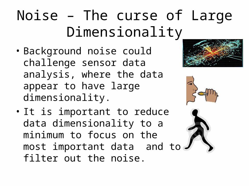
Noise – The curse of Large Dimensionality

• Background noise could challenge sensor data analysis, where the data appear to have large dimensionality.

• It is important to reduce data dimensionality to a minimum to focus on the most important data and to filter out the noise.

Reducing Dimensionality

• Principle Component Analysis (PCA)– Project data on PC’s that reflect the greatest

variance in the data– Subsequent orthogonal PC’s to capture

variance missed by first PC’s – Ignore data that are not within pc’s. they

should be considered as noise.

• PCA is good in finding new, more informative, uncorrelated features; it reduces dimensionality by rejecting low variance features

PC2

PC1

Principle Components - Example

Finding Principle Components

Looking for a transformation of the data matrix X (nxp) such that

Y= T X=1 X1+ 2 X2+..+ p Xp

Where =(1 , 2 ,.., p)T is a column vector of wheights with

1²+ 2²+..+ p² =1

Maximize the Variance: Var(T X)Good Better

Characterizing Sensor Data

• In dealing with a large amount of sensor data, it may be crucial to understand the nature of the data - that is to characterize the data in a way meaningful to the analyst.

• Clustering is a well known technique to achieve this goal.

• Also known as unsupervised learning.

Clustering Definition

Clustering is the classification of objects into different groups, or more precisely, the partitioning of a data set into subsets (clusters), so that the data in each cluster (ideally) share some common trait - often proximity according to some defined distance measure.

Example: Euclidean metric

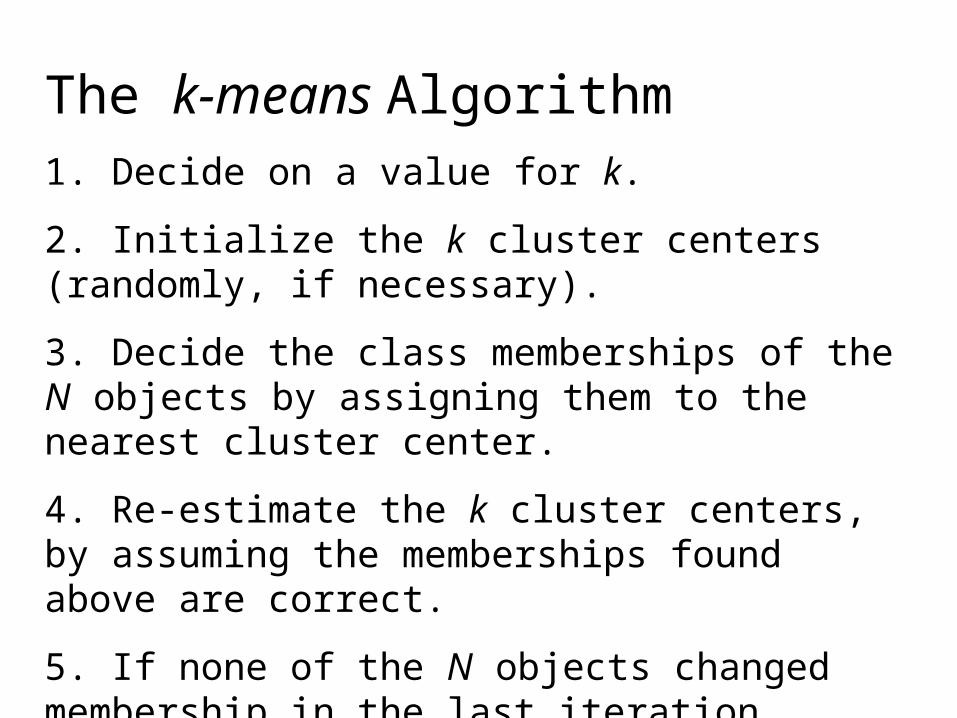
The k-means Algorithm1. Decide on a value for k.

2. Initialize the k cluster centers (randomly, if necessary).

3. Decide the class memberships of the N objects by assigning them to the nearest cluster center.

4. Re-estimate the k cluster centers, by assuming the memberships found above are correct.

5. If none of the N objects changed membership in the last iteration, exit. Otherwise go to 3.

Goal of k-means Algorithm

10

1 2 3 4 5 6 7 8 9 10

1

2

3

4

5

6

7

8

9

Objective Function

0

1

2

3

4

5

0 1 2 3 4 5

K-means Clustering: Step 1K-means Clustering: Step 1Algorithm: k-means, Distance Metric: Euclidean Distance

k1

k2

k3

0

1

2

3

4

5

0 1 2 3 4 5

K-means Clustering: Step 2K-means Clustering: Step 2Algorithm: k-means, Distance Metric: Euclidean Distance

k1

k2

k3

0

1

2

3

4

5

0 1 2 3 4 5

K-means Clustering: Step 3K-means Clustering: Step 3Algorithm: k-means, Distance Metric: Euclidean Distance

k1

k2

k3

0

1

2

3

4

5

0 1 2 3 4 5

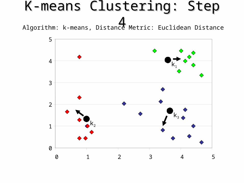
K-means Clustering: Step 4K-means Clustering: Step 4Algorithm: k-means, Distance Metric: Euclidean Distance

k1

k2

k3

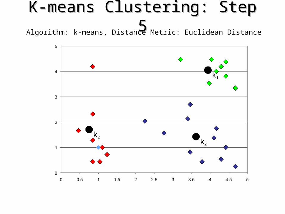
K-means Clustering: Step 5K-means Clustering: Step 5Algorithm: k-means, Distance Metric: Euclidean Distance

k1

k2k3

Pros and ConsPros and Cons

• Pros– Relatively efficient: O(tkn), where n is # objects, k is #

clusters, and t is # iterations. Normally, k, t << n.– Often terminates at a local optimum. The global optimum

may be found using techniques such as: deterministic annealing and genetic algorithms

• Cons– Applicable only when mean is defined, then what about

categorical data?– Need to specify k, the number of clusters, in advance– Unable to handle noisy data and outliers– Not suitable to discover clusters with non-convex shapes

0.00E+00

1.00E+02

2.00E+02

3.00E+02

4.00E+02

5.00E+02

6.00E+02

7.00E+02

8.00E+02

9.00E+02

1.00E+03

1 2 3 4 5 6k

Obj

ectiv

e F

unct

ion

Selecting K

For in-depth study of clustering

• Duda, R.O., Hart, P.E., Stork, D.G. Pattern classification (2nd edition), Wiley, 2001.

• Bishop , C., Pattern Recognition and Machine Learning (1st edition), Springer, 2006.

Detecting Patterns

• A form of knowledge discovery, to allow us understand the raw sensors data better, and to learn more about the phenomena generating the data

• Approach I: Association analysis (a.k.a Affinity analysis) finds frequent co-occurrences between values of raw sensors (aka frequent item set) – Frequent item sets are important patterns that can

lead to if-then rules that guides classification of future data points.

• Approach II: Episode Detection Algorithm

Example

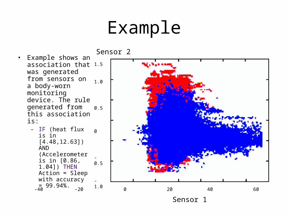
• Example shows an association that was generated from sensors on a body-worn monitoring device. The rule generated from this association is:

– IF (heat flux is in [4.48,12.63]) AND (Accelerometer is in [0.86, 1.04]) THEN Action = Sleep with accuracy = 99.94%.

-40 -20 0 20 40 60 80 100

1.5

1.0

0.5

0

-0.5

-1.0

Sensor 1

Sensor 2

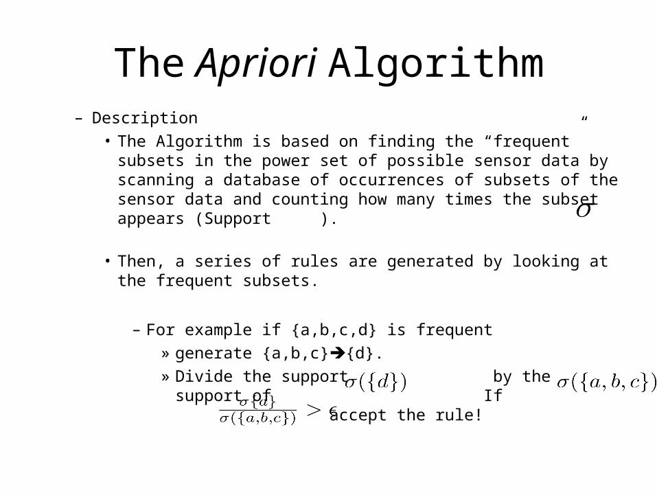
– Description• The Algorithm is based on finding the “frequent” subsets in

the power set of possible sensor data by scanning a database of occurrences of subsets of the sensor data and counting how many times the subset appears (Support ).

• Then, a series of rules are generated by looking at the frequent subsets.

– For example if {a,b,c,d} is frequent » generate {a,b,c}{d}. » Divide the support by the support of

If accept the rule!

The Apriori Algorithm

For more on Affinity Analysis

• Agrawal R, Imielinski T, Swami AN. "Mining Association Rules between Sets of Items in Large Databases." SIGMOD. June 1993, 22(2):207-16.

Episode Discovery Algorithm

• Based on: a sliding window

• .. and: the Minimum Description Length (MDL) principle– Any regularity in the data can be used to compress the

data, i.e. to describe it using fewer symbols than the number of symbols needed to describe the data literally. The more regularities there are, the more the data can be compressed

€

ti ti+1 ti+2 ti+3 ti+4 ...The sequence of time stamps for the sensor outputs

1 2 4 4 4 4 3 4 4 4 4

Classifying Sensor Data

• Unlike data clustering, classification is a supervised learning process

• Common Data Analysis goal is to map sensor data points to pre-defined class label, i.e. classifying the data.– For example, each individual in a house is a class, then we want

to map each time-ordered data to each of the individuals.

• Examples of Classifiers– Bayesian Classifiers.– Linear Classifiers.– Neural networks.– Support Vector Machines– more

Example - Linear Classifiers

Y is the outputX are the input data for a pointW are the weights for each input data

Multiple Linear Classifiers Examples

Class 1

Class 2

A Line has below points and above points, you can use that for classification.

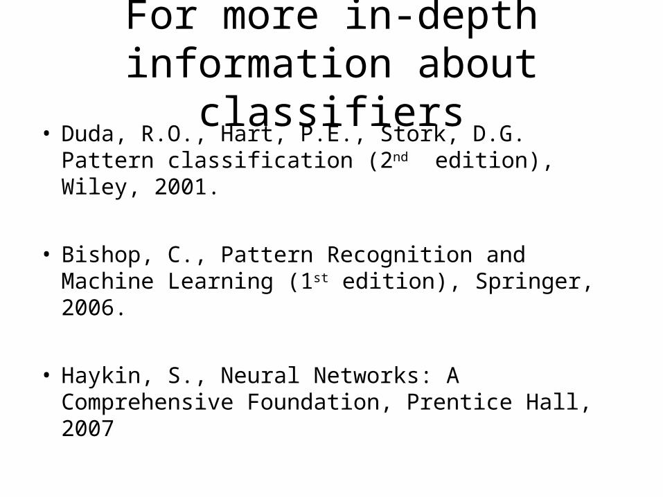
For more in-depth information about classifiers

• Duda, R.O., Hart, P.E., Stork, D.G. Pattern classification (2nd edition), Wiley, 2001.

• Bishop, C., Pattern Recognition and Machine Learning (1st edition), Springer, 2006.

• Haykin, S., Neural Networks: A Comprehensive Foundation, Prentice Hall, 2007

Detecting Trends

• Because sensor data has a time component, it can be analyzed to determine trends.– Increasing patterns.– Decreasing patterns – Cyclic patterns, – Stable patterns.

• Two main methods– Temporal Autocorrelation plots.– Anomaly Detection

Cyclic Data

Autocorrelation plot

Temporal Autocorrelation• Temporal autocorrelation refers to the correlation between time-

shifted values of a time series. It reflects the fact that the signal value at a given time point is not completely independent of its past signal values.

High Correlation

A little bit of Math

• Autocorrelation Function looks like

• E is the expectation.

• represents the signal at time t.

• represents the shifted signal at a different time s.

Then the process can be seen as…

• Trying to match the signal that you have against a shifted version of the same signal with respect to time.

For more information

• Denning, D., "An Intrusion Detection Model," Proceedings of the Seventh IEEE Symposium on Security and Privacy, May 1986, pages 119-131.

• Teng, H. S., Chen, K., and Lu, S. C-Y, "Adaptive Real-time Anomaly Detection Using Inductively Generated Sequential Patterns," 1990 IEEE Symposium on Security and Privacy

• Jones, A. K., and Sielken, R. S., "Computer System Intrusion Detection: A Survey," Technical Report, Department of Computer Science, University of Virginia, Charlottesville, VA, 1999

Phenomena Clouds

• A phenomenon cloud P is expressed as a 5-tuple:

P = <a, b, pT, m, n>; where:

[a, b] defines the range of magnitude of the phenomenon,

pT defines threshold probability,

m defines sliding window size and,

n defines minimum quorum.

Classification of Roles assigned to Sensors

• Tracking

• Candidate

• Potential Candidate

• Idle

Role Transition Rules• R1: Candidate → Tracking: If a sensor satisfies the Phenomenon-Condition then it transitions into the tracking category.

• R2: Potential Candidate → Candidate: A potential candidate sensor will transition to a candidate sensor if any of its neighbors transitions into a tracking sensor.

• R3: Idle → Potential Candidate: An idle sensor transitions into a potential candidate if any of its neighbors becomes a candidate sensor.

• R4: Tracking → Candidate: A tracking sensor will transition down to the candidate category; if it is unable to satisfy the Phenomenon-Condition.

• R5: Candidate → Potential Candidate: A candidate sensor will transition to a potential candidate sensor if none of its neighbors are tracking sensors.

• R6: Potential Candidate → Idle: A potential candidate transitions into an idle sensor if all its neighbors are either potential candidates or idle, that is none of its neighbors are in the candidate category.

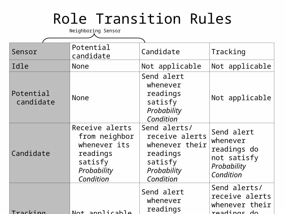
Role Transition Rules

Sensor Potential candidate Candidate Tracking

Idle None Not applicable Not applicable

Potential candidate None

Send alert whenever readings satisfy Probability Condition

Not applicable

Candidate

Receive alerts from neighbor whenever its readings satisfy Probability Condition

Send alerts/ receive alerts whenever their readings satisfy Probability Condition

Send alert whenever readings do not satisfy Probability Condition

Tracking Not applicable

Send alert whenever readings satisfy Probability Condition

Send alerts/ receive alerts whenever their readings do not satisfy Probability Condition

Neighboring Sensor

Steps in the Detection & Tracking ProcessInitial Selection &

Monitoring Initial OccurrenceGrowth of Phenomenon

Cloud

Idle Sensor Potential Candidate

CandidateTracking

Shrinking of Phenomenon Cloud

A Practical Demonstration of Phenomena Detection and Tracking

Gator Tech Smart House (GTSH)

Smart Floor

Effect of a Footstep on the Smart Floor

Experimental Analysis - Detection Performance

Effect of varying quorum ‘n’ on detection performance

Pervasive & Ubiquitous Systems

The Role of Computational Intelligence in Pervasive Spaces

• Learn over time from user interactions and behavior, and from the environment

• Robustly manage User Uncertainty– Intra-User Uncertainty: user approach same problem differently

over time– Inter-User uncertainty: different users approach same problem

differently.

• Similarly, robustly manage environmental uncertainty such as noise, change of season etc.

CI techniques are tolerant to imprecision, uncertainty, approximation, and partial truths.

Three widely used techniques in Computational Intelligence

• Fuzzy Systems– They mimic the human gray-logic.

• Neural Networks – They are function approximation devices.

• Evolutionary Systems– They mimic the evolutionary abilities of complex

organisms.

Fuzzy Systems

• They mimic human gray logic– We do not say

“If the temperature is above 24 degrees and the cloud cover is less than 10 percent, and I have three hours time, I will go for a hike with a probability of 0.47.”

– We say “If the weather is nice and I have a little time, I will probably go for a walk.”

Type-1 fuzzy sets

• Definition

A fuzzy set is a pair (A,m) where A is a set

and

This function m represent the confidence of an element in the fuzzy set (A,m).

Example: Represent Linguistic Variables

• Quality of a car in a scale from 0-1000

Relationship to Boolean Logic

• The Boolean set is a special case of the fuzzy set.

• No crisp boundaries between the different fuzzy sets. This means

that paradox are acceptable.

– For example, a plate can be cold and hot at the same time.

Fuzzy Logic as a Generalization of Boolean Logic

• Union is the operator max

• Intersection is the operator min

• Complement is defined as

• Implication rule

Example• Assume the set of temperatures with range 0 to 35

Celsius, we have the following fuzzy sets

0 5 10 15 20 25 30 350

0.1

0.2

0.3

0.4

0.5

0.6

0.7

0.8

0.9

1

Temperature Co

Cold Membership

Cold

0 5 10 15 20 25 30 350

0.1

0.2

0.3

0.4

0.5

0.6

0.7

0.8

0.9

1

Temperature CoWarm Membership

Warm

0 5 10 15 20 25 30 350

0.1

0.2

0.3

0.4

0.5

0.6

0.7

0.8

0.9

1

Temperature Co

Hot Membership

Hot

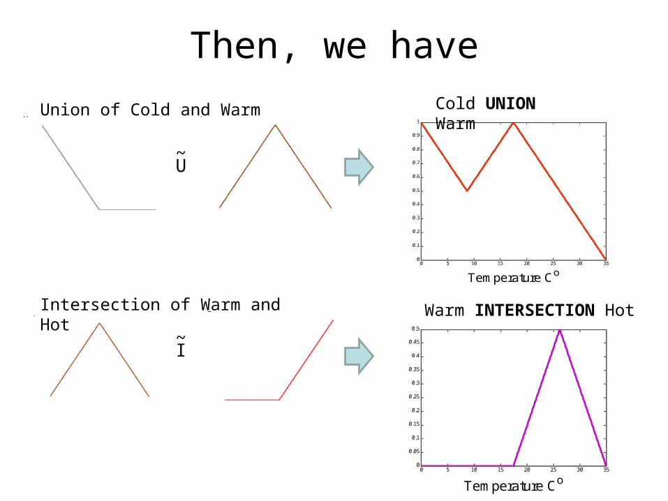
Then, we have

Union of Cold and Warm

0 5 10 15 20 25 30 350

0.1

0.2

0.3

0.4

0.5

0.6

0.7

0.8

0.9

1

Temperature Co

Cold Membership

0 5 10 15 20 25 30 350

0.1

0.2

0.3

0.4

0.5

0.6

0.7

0.8

0.9

1

Temperature CoWarm Membership

U~

0 5 10 15 20 25 30 350

0.1

0.2

0.3

0.4

0.5

0.6

0.7

0.8

0.9

1

Temperature Co

Cold UNION Warm

Intersection of Warm and Hot

0 5 10 15 20 25 30 350

0.1

0.2

0.3

0.4

0.5

0.6

0.7

0.8

0.9

1

Temperature CoWarm Membership

0 5 10 15 20 25 30 350

0.1

0.2

0.3

0.4

0.5

0.6

0.7

0.8

0.9

1

Temperature Co

Hot Membership

I~

Warm INTERSECTION Hot

0 5 10 15 20 25 30 350

0.05

0.1

0.15

0.2

0.25

0.3

0.35

0.4

0.45

0.5

Temperature Co

Cont…Complement Hot

0 5 10 15 20 25 30 350

0.1

0.2

0.3

0.4

0.5

0.6

0.7

0.8

0.9

1

Temperature Co

Hot Membership

0 5 10 15 20 25 30 350

0.1

0.2

0.3

0.4

0.5

0.6

0.7

0.8

0.9

1

Temperature Co

Quasi – Cold Warm?

¬

Now the Implication Cold→Warm

0 5 10 15 20 25 30 350

0.1

0.2

0.3

0.4

0.5

0.6

0.7

0.8

0.9

1

Temperature Co

0 5 10 15 20 25 30 350

0.1

0.2

0.3

0.4

0.5

0.6

0.7

0.8

0.9

1

Temperature Co

Cold Membership

0 5 10 15 20 25 30 350

0.1

0.2

0.3

0.4

0.5

0.6

0.7

0.8

0.9

1

Temperature CoWarm Membership

Utility of Fuzzy Systems

• They mimic the gray human logic

• Linguistic variables can be easily mapped into real values

• Implement rule services that can be used by applications. – E/C/A models can utilize fuzzy rules providing

a much more human-like and smoother reactivity to events

Limitations of Type 1 Fuzzy Sets

• They handle short term uncertainties very well. For instance: – Slight noise and imprecision associated with sensors and

actuators.– Slight user-behavior variations.

• Long-term uncertainties (e.g., aging models) will degrade the effectiveness of type-1 based Fuzzy Logic Systems.

• Type-2 fuzzy sets handles longer term uncertainties

Type-2 Fuzzy Sets

• Type-2 fuzzy sets have grades of membership that are themselves fuzzy.

Type-2 Fuzzy Set with fuzzy Gaussian membership.

Type-2 Fuzzy Sets Advantages

• They handle long term uncertainties better because the membership value itself is a fuzzy function.

• The fussy systems based on type-2 fuzzy sets need less rules to work compared to the type-1 fuzzy sets based systems.

Deployment of Fuzzy Logic Systems

• University of Zurich• Office building at the university.• Type-1 FLSs are employed as multiple agents

controlling subparts of the environment.

• University of Essex• iDorm• Unsupervised techniques are used for learning abd

extracting the fuzzy membership functions and rules that represent and model behaviors in the environment that are particular to a user.

Neural Networks

• This computing paradigm is loosely modeled after the brain’s cortical structures and the central nervous system.

• Such networks consist of interconnected processing

elements called neurons that work together to produce an output function.

• The most commonly used model is the multilayer perceptron

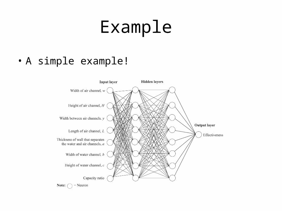
Example

• A simple example!

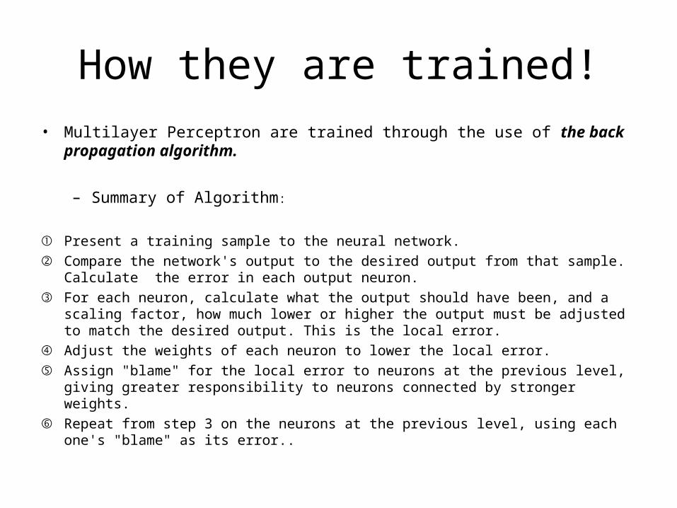
How they are trained!

• Multilayer Perceptron are trained through the use of the back propagation algorithm.

– Summary of Algorithm:

① Present a training sample to the neural network.

② Compare the network's output to the desired output from that sample. Calculate the error in each output neuron.

③ For each neuron, calculate what the output should have been, and a scaling factor, how much lower or higher the output must be adjusted to match the desired output. This is the local error.

④ Adjust the weights of each neuron to lower the local error.

⑤ Assign "blame" for the local error to neurons at the previous level, giving greater responsibility to neurons connected by stronger weights.

⑥ Repeat from step 3 on the neurons at the previous level, using each one's "blame" as its error..

Neural Network based Deployments

• University of Colorado – Adaptive Smart House

• To control the environment inside of the house to increase comfort and improve power saving.

• Researchers have also employed neural networks in pervasive living spaces to identify patterns of behavior and alterations in those patterns to better support care systems.

Evolutionary Systems

• Examples– Genetic Algorithms

– Learning Classifier Systems

– Evolutionary Programming

– Swarm Intelligence

Swarm intelligence

Example

The ant colony optimization algorithm (ACO), introduced by Marco Dorigo in 1992 in his PhD thesis, is a probabilistic technique for solving computational problems which can be reduced to finding good paths through graphs.

It is inspired by the behavior of ants in finding paths from the colony to food.

Using Swarm Intelligence in Pervasive Spaces

• You could think of each sensor as an ant, and of goals (or contexts) as end of a path that ant will take. – For instance, floor pressure sensors are ants and detetcing walking

patterns are paths.

• The system takes time to evolves and allows these paths to be discovered.