sensor networks acoe 422 adopted from ieee tutorial on sensor networks
TRANSCRIPT
Sensor Networks
ACOE 422
Adopted from IEEE Tutorial on Sensor Networks
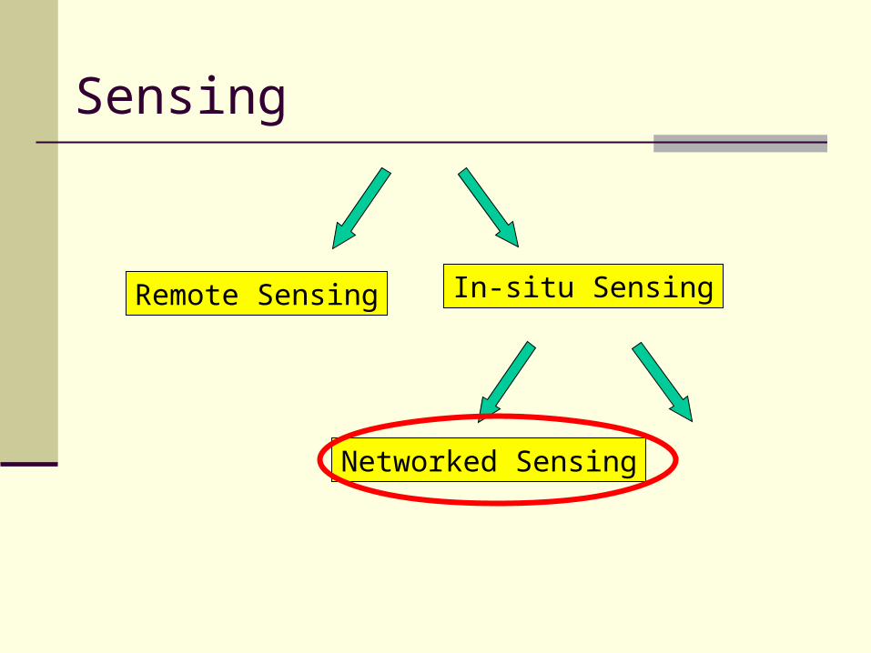
Sensing
Remote Sensing In-situ Sensing
Networked Sensing
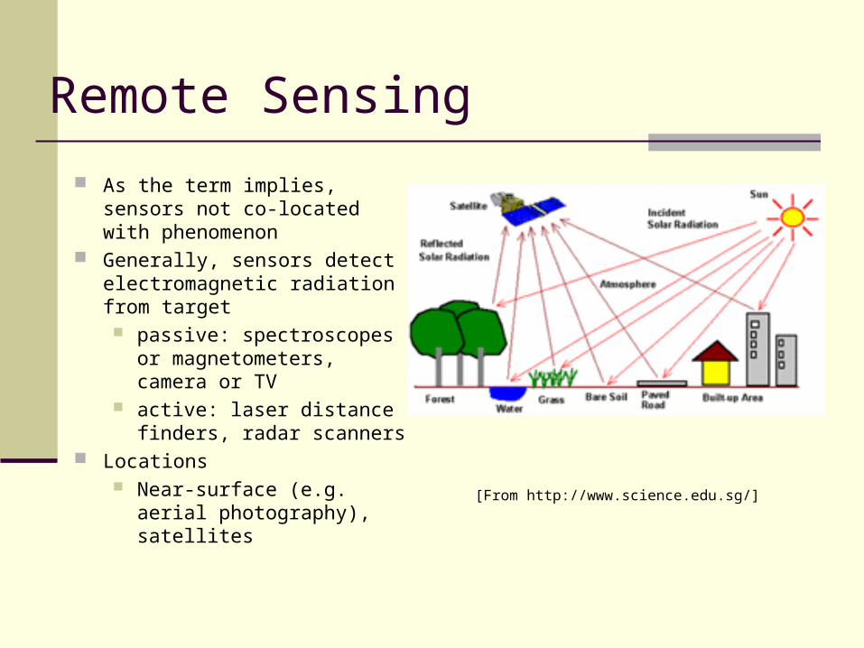
Remote Sensing
As the term implies, sensors not co-located with phenomenon
Generally, sensors detect electromagnetic radiation from target passive: spectroscopes or
magnetometers, camera or TV active: laser distance finders,
radar scanners Locations
Near-surface (e.g. aerial photography), satellites [From http://www.science.edu.sg/]
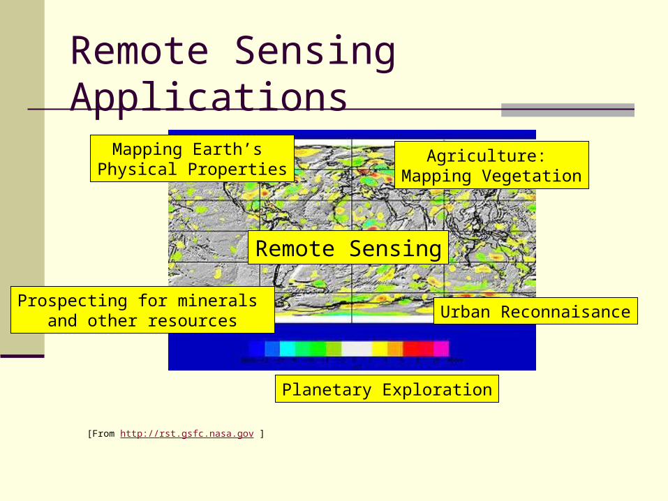
Remote Sensing Applications
Remote Sensing
Mapping Earth’s Physical Properties
Prospecting for minerals and other resources
Agriculture: Mapping Vegetation
Urban Reconnaisance
Planetary Exploration
[From http://rst.gsfc.nasa.gov ]

Remote SensingAnalysis and Systems Analysis: mostly image-processing
related spectral analysis image filtering classification (maximum
likelihood) principal components analysis
Systems GIS: Geographic Information
Systems Flexibly combine various
images
[From http://erg.usgs.gov/ ]

In-situ Sensing
Sensors situated close to phenomena accurate, microscopic
observations … but with limited range
General uses in engineering applications Condition monitoring Performance tuning
[From http://www.sensorland.com/ ]
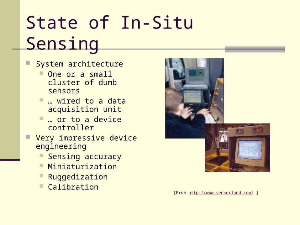
State of In-Situ Sensing
System architecture One or a small cluster of
dumb sensors … wired to a data
acquisition unit … or to a device controller
Very impressive device engineering Sensing accuracy Miniaturization Ruggedization Calibration
[From http://www.sensorland.com/ ]

Current Applications
Agriculture Plant positioning Precision hoeing
Automotive, highway systems Engine pressure and oxygen
monitoring Suspension positioning of racing cars
and motorcycles Road noise measurements
Aviation Aircraft engine pressure
Entertainment Rotational stability of Ferris wheels Acoustic adjustments in symphony
halls
Manufacturing processes Humidity in compressed air Tail-lift testing Fan pitch monitoring Calibrating bullet speeds
Railways Braking control load distribution Traction control in slippery
conditions Shipping
Rudder positioning Space
Rocket engine valve positioning Utilities
Water distribution and storage
Industry
Many, many sensor manufacturers Sensor Magazine’s buying
guide lists 240 manufacturers of acceleration measurement sensors!
Some names Agilent, Wilcoxon,
Crossbow, GEMS, Penny and Giles, Delphi, Motorola, ScanTek, Bosch, National Instruments
The applicability of sensors is vast …
Companies often stratified by Industry segment (e.g.
Delphi automotive) Application (e.g. vibration
measurement, or pressure measurement)
… and differentiate themselves by offering a wide range of
products with different specifications or differing form factors

Standardization
Fair amount of activity since the mid-1990s IEEE P1451.x
Two thrusts: Sensor board to processor
interfaces wired/wireless bus,
point-to-point both for data access and
sensor self-identification
Object-oriented abstractions for sensor data and application interaction
[From Plug-and-Play Sensors Sensors Magazine, December 02]

Sensing
Remote Sensing In-situ Sensing
Networked Sensing

Networked Sensing Enabler
Small (coin, matchbox sized) nodes with Processor
8-bit processors to x86 class processors
Memory Kbytes – Mbytes range
Radio 20-100 Kbps initially
Battery powered Built-in sensors!

The Opportunity
Large-scale fine-grain in-situ sensing and actuation 100s to 1000s of nodes 5m to 50m spacing
Inherently collaborative … sensors cannot act alone because they have limited view
Inherently distributed … since communication is energy-intensive (we’ll see this later)
Embedded (In-Situ) Networked Sensing
Applications

Application Areas
Seismic Structure Response
Contaminant Transport
Marine Microorganisms
Ecosystems, Biocomplexity
Structural Condition Assessment

Seismic Structure Response
Interaction between ground motions and structure/foundation response not well understood.
Current seismic networks not spatially dense enough to monitor structure
deformation in response to ground motion.
to sample wavefield without spatial aliasing.
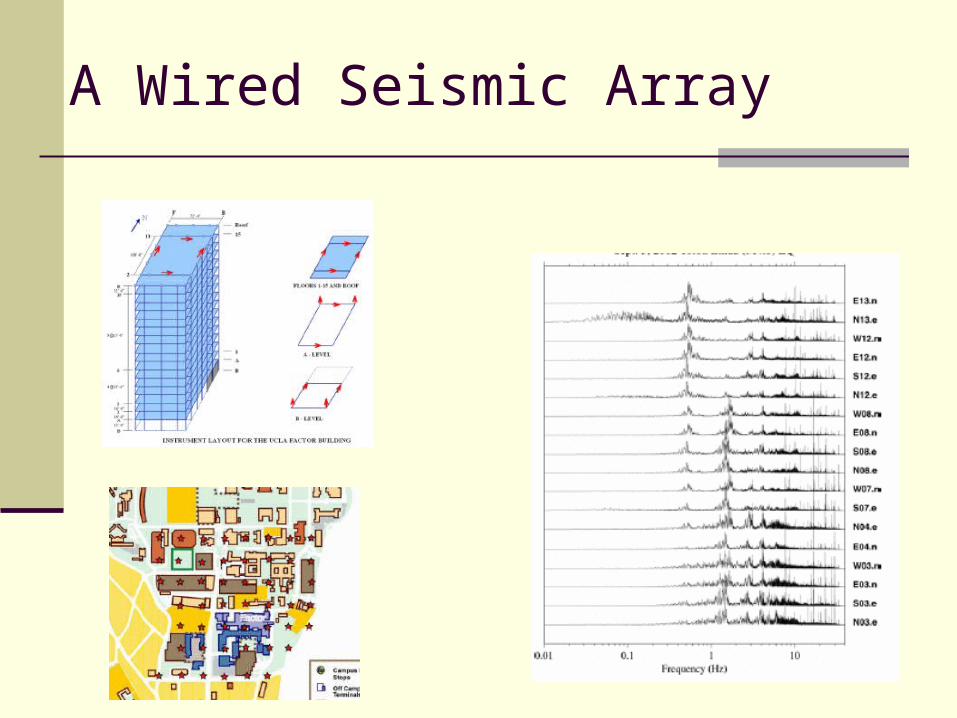
A Wired Seismic Array
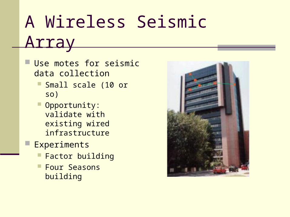
A Wireless Seismic Array
Use motes for seismic data collection Small scale (10 or so) Opportunity: validate
with existing wired infrastructure
Experiments Factor building Four Seasons building
Condition Assessment
Longer-term Challenges:
Detection of damage (cracks) in structures
Analysis of stress histories for damage prediction
Applicable not just to buildings Bridges, aircraft

Contaminant Transport
Industrial effluent dispersal can be enormously damaging to the environment marine contaminants groundwater contaminants
Study of contaminant transport involves Understanding the physical (soil
structure), chemical (interaction with and impact on nutrients), and biological (effect on plants and marine life) aspects of contaminants
Modeling their transports Mature field! Fine-grain sensing can help
Responsible Party contributions for cleanup of “Superfund” sites (source: U.S. EPA, 1996)
1 9 8 0 1 9 8 5 1 9 9 0 1 9 9 5 0
42
681012
Bil
lion
s of
dol
lars

Lab-Scale Experiments
Use surrogates (e.g. heat transfer) to study contaminant transport
Testbed Tank with heat source
and embedded thermistors
Measure and model heat flow
[From CENS Annual Technical Report, 03]

Field-Level Experiments
Nitrates in groundwater Application
Wastewater used for irrigating alfalfa
Wastewater has nitrates, nutrients for alfalfa
Over-irrigation can lead to nitrates in ground-water
Need monitoring system, wells can be expensive
Pilot study of sensor network to monitoring nitrate levels
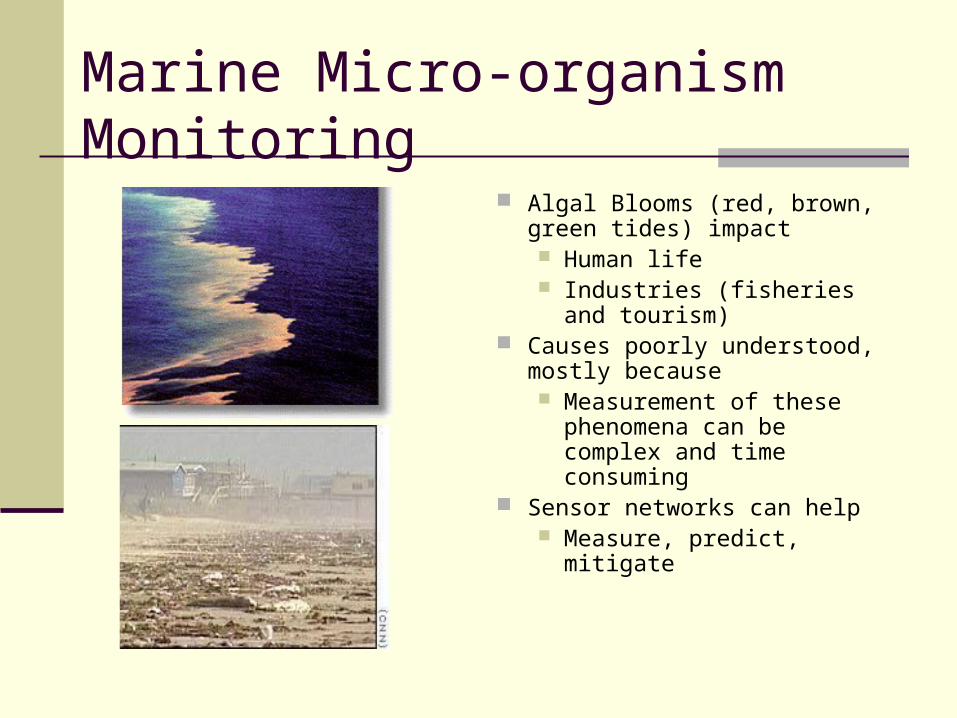
Marine Micro-organism Monitoring
Algal Blooms (red, brown, green tides) impact Human life Industries (fisheries and
tourism) Causes poorly understood,
mostly because Measurement of these
phenomena can be complex and time consuming
Sensor networks can help Measure, predict, mitigate

Lab-Scale Experimentation
Build a tank testbed in which to study the factors that affect micro-organism growth
Actuation is a central part of this Can’t expect to deploy at
density we need Mobile sensors can help
sample at high frequency Initial study:
thermocline detection
1m
Tethered-robot sample
collectors

Ecosystem Monitoring
Remote sensing can enable global assessment of ecosystem
But, ecosystem evolution is often decided by local variations Development of canopy, nesting patterns often
decided by small local variations in temperature In-situ networked sensing can help us understand
some of these processes
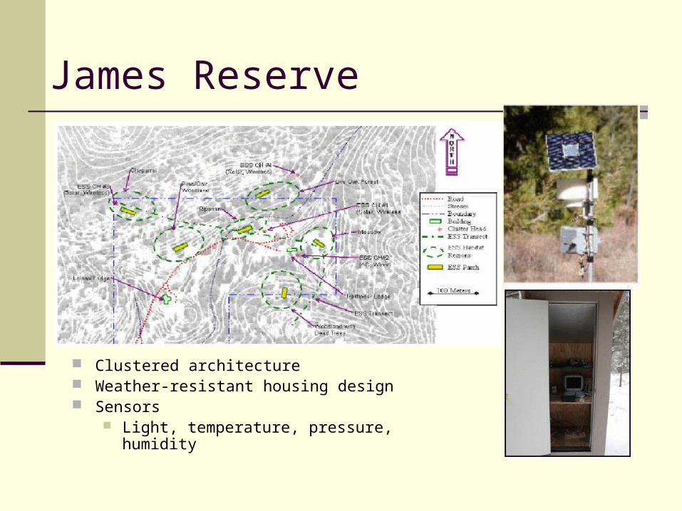
James Reserve
Clustered architecture Weather-resistant housing design Sensors
Light, temperature, pressure, humidity

Great Duck Island
Study nesting behavior of Leach’s storm petrels
Clustered architecture: 802.11 backbone multihop sensor cluster
Now running for several months
Base-Remote Link
Data Service
Internet
Client Data Browsing and Processing
Transit Network
Basestation
Gateway
Sensor Patch
Patch Network
Sensor Node

Challenges and Goals

Networked Sensing Challenges
Energy is a design constraint Network lifetime now becomes a metric
Interaction with the physical world A lot messier than we’ve been used to
Autonomous deployment We’re not used to building systems that can self-deploy
Single (or a small number) of users Need a different model

Communication is Expensive
The Communication/Computation Tradeoff Received power drops off as the fourth power of distance
10 m: 5000 ops/transmitted bit 100 m: 50,000,000 ops/transmitted bit Gets networking and distributed systems researchers excited! At short transmission ranges, reception costs are significant
Implications Avoid communication over long distances Cannot assume global knowledge, or centralized solutions Can leverage data processing/aggregation inside the networkCan leverage data processing/aggregation inside the network
Communication is Expensive The Communication/Computation Tradeoff
Received power drops off as the fourth power of distance
10 m: 5000 ops/transmitted bit 100 m: 50,000,000 ops/transmitted bit Gets networking and distributed systems researchers excited! At short transmission ranges, reception costs are significant
Implications Avoid communication over long distances Cannot assume global knowledge, or centralized solutions Can leverage data processing/aggregation inside the networkCan leverage data processing/aggregation inside the network

The Goal
An infrastructure that can be used by many different sensing applications

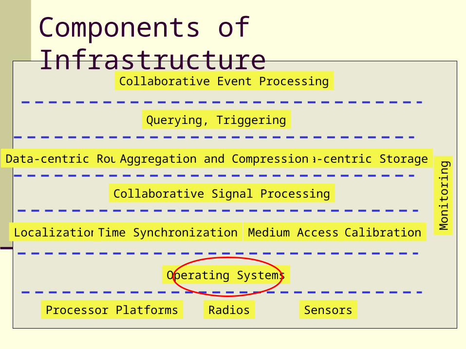
Components of Infrastructure
Processor Platforms Radios Sensors
Operating Systems
Localization Time Synchronization Medium Access Calibration
Collaborative Signal Processing
Data-centric Routing Data-centric Storage
Querying, Triggering
Aggregation and Compression
Collaborative Event Processing
Mon
itor
ing
Secu
rity

Tutorial Overview
Discuss components bottom-up Present a networking and systems view In each topic
Present relatively mature systems (to the extent they exist) first
Then discuss systems research Finally, present some theoretical underpinnings

Hardware: Platforms, Radios and Sensors
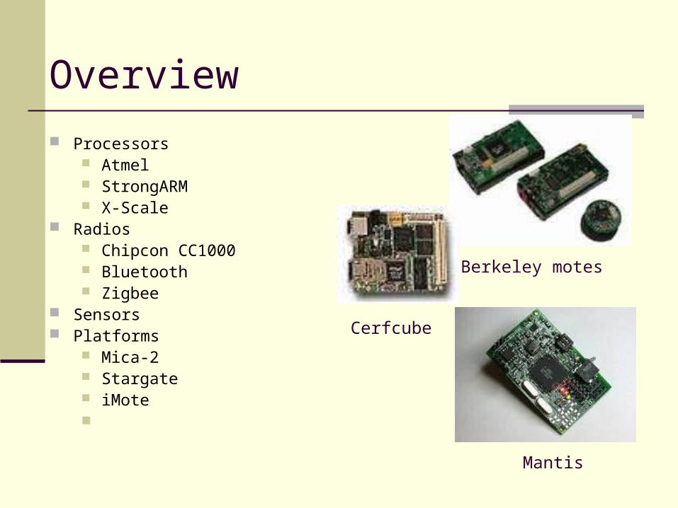
Overview
Berkeley motes
Mantis
Cerfcube
Processors Atmel StrongARM X-Scale
Radios Chipcon CC1000 Bluetooth Zigbee
Sensors Platforms
Mica-2 Stargate iMote
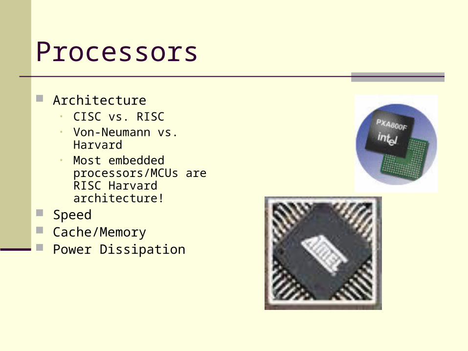
Processors
Architecture • CISC vs. RISC • Von-Neumann vs. Harvard • Most embedded
processors/MCUs are RISC Harvard architecture!
Speed Cache/Memory Power Dissipation

Atmel Atmega 128L
Harvard 8-bit RISC Speed : 8MHz Memory:
128KB program memory 4KB SRAM 4KB EEPROM
Power draw: run mode: 16.5mW sleep mode: < 60µW
Microcontroller used in Mica2

Intel StrongARM SA1100
Harvard 32-bit RISC Speed: 206MHz Cache:
16KB instruction cache 8KB data cache
Power draw: run mode : 800mW idle mode : 210mW sleep mode : 50µW
Microprocessor used in iPAQ H3700

Intel XScale PXA-250
A successor to the StrongARM Harvard 32-bit RISC Speed : 200/300/400MHz Cache:
32KB instruction cache 32 KB data cache
Power draw: run mode : 400mW idle mode : 160mW sleep mode : 50µW
Microprocessor used in iPAQ H3900
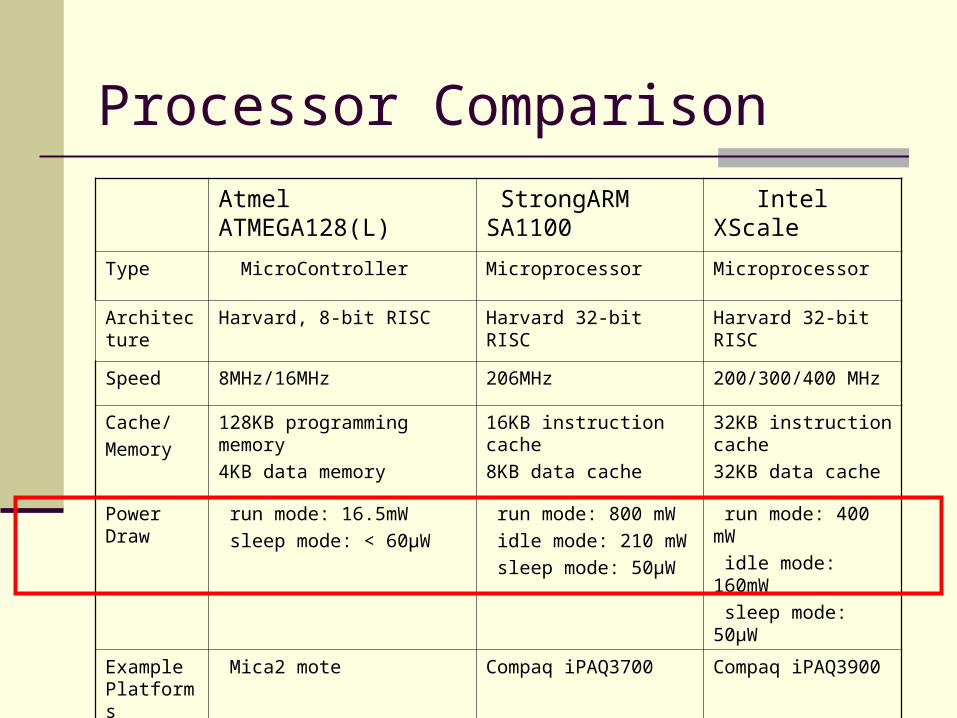
Atmel ATMEGA128(L) StrongARM SA1100
Intel XScale
Type MicroController Microprocessor Microprocessor
Architecture Harvard, 8-bit RISC Harvard 32-bit RISC Harvard 32-bit RISC
Speed 8MHz/16MHz 206MHz 200/300/400 MHz
Cache/
Memory
128KB programming memory
4KB data memory
16KB instruction cache
8KB data cache
32KB instruction cache
32KB data cache
Power Draw run mode: 16.5mW
sleep mode: < 60µW
run mode: 800 mW
idle mode: 210 mW
sleep mode: 50µW
run mode: 400 mW
idle mode: 160mW
sleep mode: 50µW
Example Platforms
Mica2 mote Compaq iPAQ3700 Compaq iPAQ3900
Processor Comparison
Radios
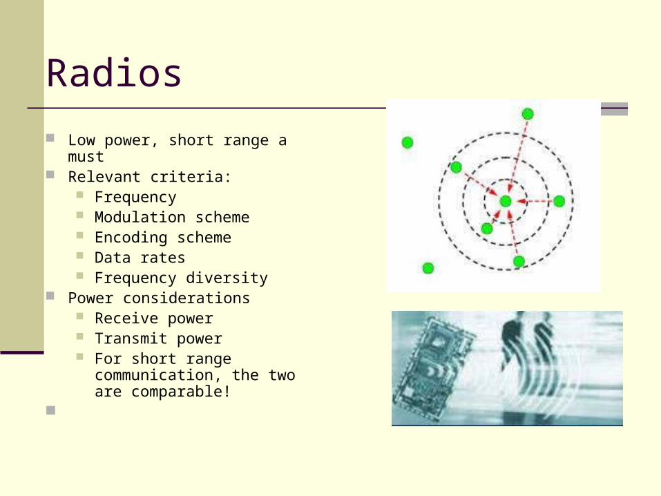
Low power, short range a must Relevant criteria:
Frequency Modulation scheme Encoding scheme Data rates Frequency diversity
Power considerations Receive power Transmit power For short range
communication, the two are comparable!

[From http://www.rfm.com]
RFM TR1000
OOK/ASK 433/916 MHz Date rate up to 115.2Kbps Power draw:
Rx: 3.8mA Tx:12mA
No spread spectrum support Used in earlier platforms
Now largely obsolete
[From http://www.chipcon.com]
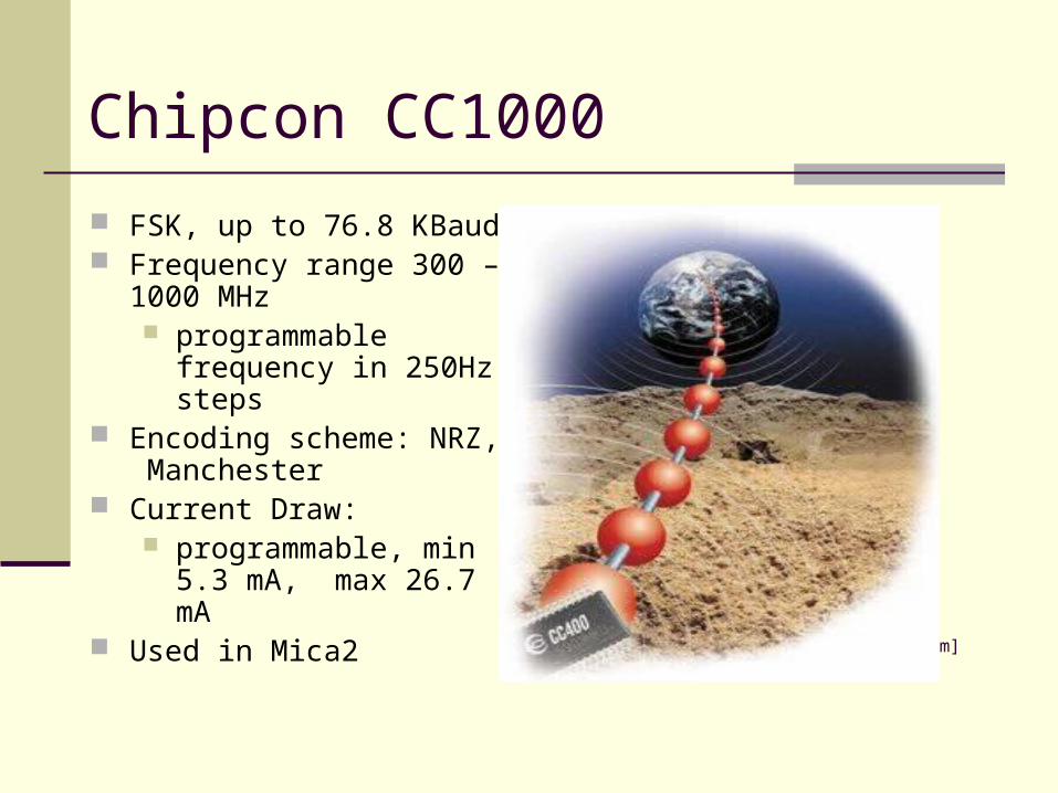
Chipcon CC1000
FSK, up to 76.8 KBaud Frequency range 300 – 1000
MHz programmable frequency in
250Hz steps Encoding scheme: NRZ,
Manchester Current Draw:
programmable, min 5.3 mA, max 26.7 mA
Used in Mica2

Bluetooth
Modulation Gaussian Filtered FSK (GFSK) 2.4GHz (ISM)
Diversity coding Frequency Hopping Spread
Spectrum. Power consumption:
Transmit: 150 mW Receive: 90 mW
Gross data rate: 6-12 KBps Point-to-point and point-to-multipoint
protocols. up to 8 devices per piconet
IEEE 802.15.4
Carriers and Modulation 868 Mhz, 900 Mhz ISM, 2.5 Ghz
ISM Different modulations at different
frequencies Diversity coding
Direct sequence MAC layer
CSMA/CA Status
Standards complete, radios expected soon
Zigbee Alliance is pushing for this Home and industrial automation They have defined a simple topology
construction/routing layer on top of this

Sensors
We describe some of the sensors types commonly used in some of our applications Theory of operation Performance parameters

[From Sensors Magazine, “How to Select and Use the Right Temperature Sensor”]
Temperature Sensor
Operation Change in resistance
induced by temperature change
Semiconductor or metal Differential changes in
resistance Thermocouples,
thermopiles Parameters
Temperature range Linearity Resolution (sensitivity)

Photo Sensors
Operation Uses Photoconductive material
Resistance decreases with increase in light
Parameters Peak Sensitivity Wavelength Illuminance Range Ambient Temperature
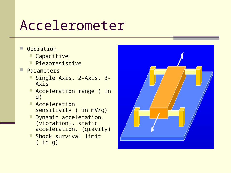
Accelerometer
Operation Capacitive Piezoresistive
Parameters Single Axis, 2-Axis, 3-Axis Acceleration range ( in g) Acceleration sensitivity ( in
mV/g) Dynamic acceleration.
(vibration), static acceleration. (gravity)
Shock survival limit ( in g)

Displacement Sensors (LVDT)
Operation Iron core between Primary
and Secondary Coils Displacement causes
voltage output Parameters
Range Linearity Sensitivity
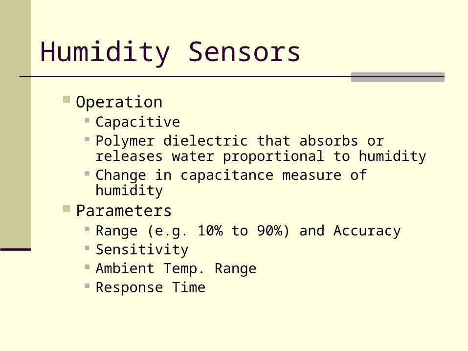
Humidity Sensors
Operation Capacitive Polymer dielectric that absorbs or releases water
proportional to humidity Change in capacitance measure of humidity
Parameters Range (e.g. 10% to 90%) and Accuracy Sensitivity Ambient Temp. Range Response Time

Magnetic Field Sensor
Operation Ferro-magnetic material (e.g. iron, nickel, cobalt) change
shape and size when placed in a Magnetic Field Parameters
Number of axes ( one, two, three) – direction of magnetic field
Range (Gauss) Noise Sensitivity Linearity Sensitivity (V/Gauss)
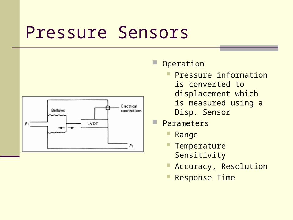
Pressure Sensors
Operation Pressure information is
converted to displacement which is measured using a Disp. Sensor
Parameters Range Temperature Sensitivity Accuracy, Resolution Response Time

Platforms
Several platforms in the community Various combinations of the processors, radios and
sensors discussed so far
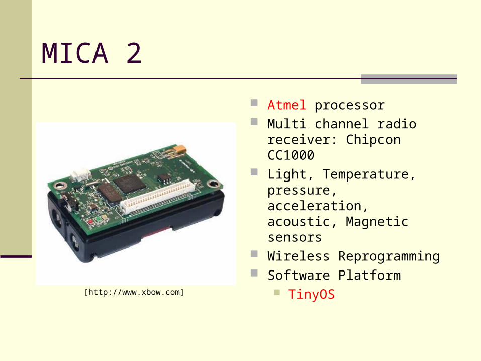
MICA 2
Atmel processor Multi channel radio receiver:
Chipcon CC1000 Light, Temperature, pressure,
acceleration, acoustic, Magnetic sensors
Wireless Reprogramming Software Platform
TinyOS
[http://www.xbow.com]
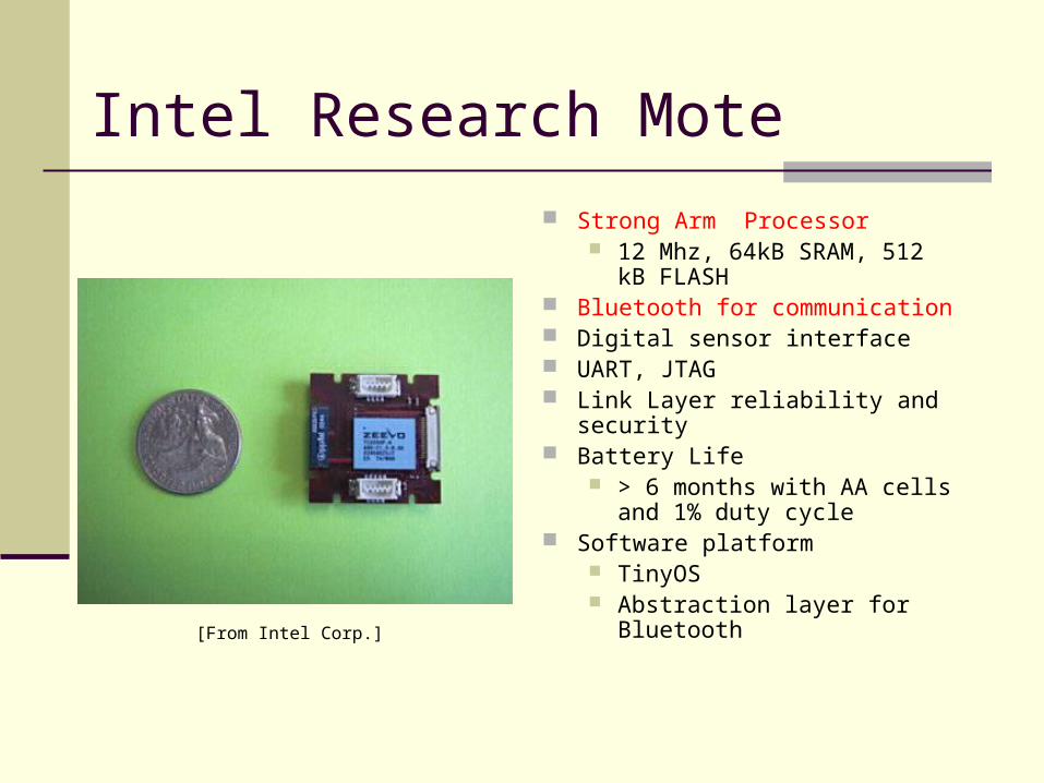
Intel Research Mote
Strong Arm Processor 12 Mhz, 64kB SRAM, 512 kB
FLASH Bluetooth for communication Digital sensor interface UART, JTAG Link Layer reliability and security Battery Life
> 6 months with AA cells and 1% duty cycle
Software platform TinyOS Abstraction layer for Bluetooth [From Intel Corp.]

Stargate
High Processing Node (Gateway)
400Mhz Xscale processor, 64MB RAM, 32MB Flash
3.5'' x 2.5 '' Ethernet, UART, JTAG, USB
via daughter card Connectors for sensor boards Standard Mica2 Connector Software Platform
Linux
[From Crossbow Inc., http://www.xbow.com]
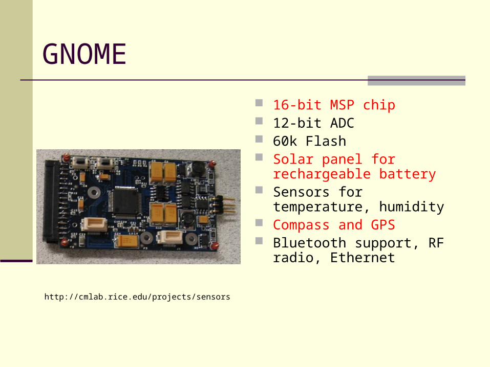
GNOME
16-bit MSP chip 12-bit ADC 60k Flash Solar panel for rechargeable
battery Sensors for temperature,
humidity Compass and GPS Bluetooth support, RF radio,
Ethernet
http://cmlab.rice.edu/projects/sensors

Medusa MK-2
High Capability node Two Microcontrollers
8-bit RISC Atmega 128L 4MHz, 32k Flash, 4kb RAM, JTAG, UART
32-bit RISC, 40MHz, 1MB Flash, 136KB RAM, JTAG, UART, GPS
They communicate via UART On Board Power Mgmt. And
Tracking Unit

Medusa MK-2
Power consumption 200 mW (fully operational)
RF Radio compatible with Mica motes
Two accessory board for ultrasonic distance measurement
Software Platform PALOS (power aware light
weight OS) Event Driven Priority Support
[http://nesl.ee.ucla.edu]

MANTIS
Hardware: The Nymph Chipcon CC1000 10 bit ADC GPS Support UART and JTAG
interface 3.5 x 5.5 sq. cm Support for up to 8
batteries
[http://mantis.cs.colorado.edu]

MANTIS
MOS Unix like development and
runtime environment Multithreaded with priority
support. But Round-Robin (not event driven)
New H/w addition via a new H/w driver
Remote login and reprogramming via wired and wireless
[http://mantis.cs.colorado.edu]
Components of Infrastructure
Processor Platforms Radios Sensors
Operating Systems
Localization Time Synchronization Medium Access Calibration
Collaborative Signal Processing
Data-centric Routing Data-centric Storage
Querying, Triggering
Aggregation and Compression
Collaborative Event Processing
Mon
itor
ing
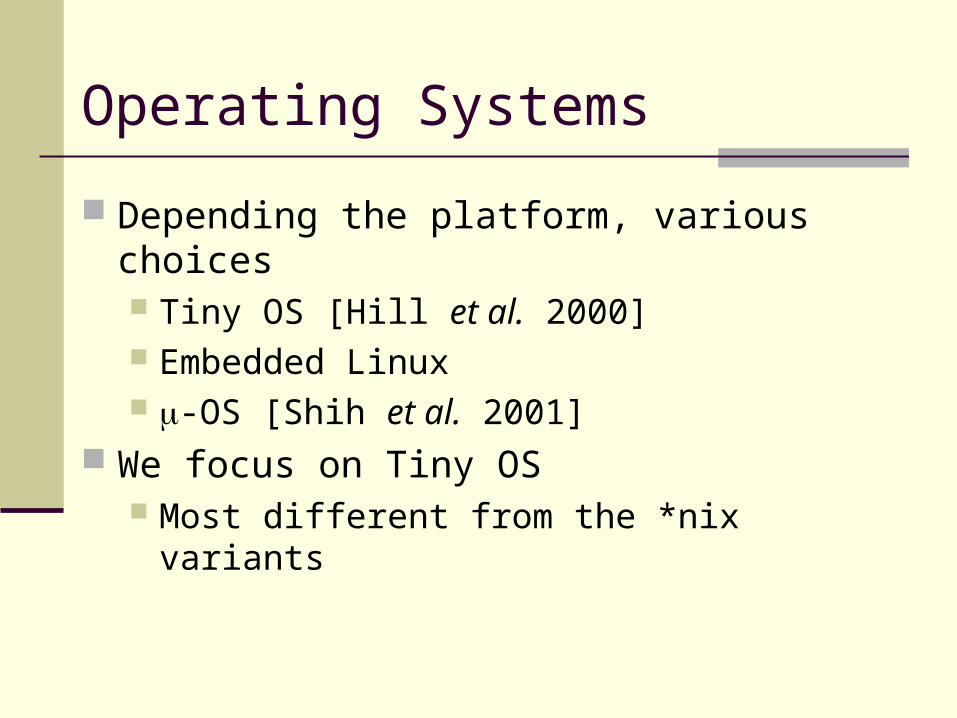
Operating Systems
Depending the platform, various choices Tiny OS [Hill et al. 2000] Embedded Linux -OS [Shih et al. 2001]
We focus on Tiny OS Most different from the *nix variants

TinyOS
De-facto sensor programming platform Initially developed by UC-Berkeley History
v0.5.1 – released at 10/19/2001 v0.6.0 – released at 02/13/2002 v0.6.1 – released at 05/10/2002 v1.0.0 – released at 10/14/2002 v1.1.0 – released at 09/23/2003

H/W Platforms using TinyOS
Crossbow Mica Crossbow Mica2 Intel Mote
CPU ATmega128L ATmega128L(4MHz) ARM core(12MHz)
Program Memory
128k Flash memory
128k Flash memory 512k Flash memory
Data Memory
4k SRAM 4k SRAM 64k SRAM
Radio RFM TR1000 ChipCon CC1000 Bluetooth
Data Rate 40 kbps 76.8 kBaud 1 Mbps
Frequency 916.50 MHz 315/433/868/915MHz
2.4GHz

TinyOS Programming Model
Event-driven execution no polling, no blocking
Concurrency intensive operation multi-threads based, no long-running thread
Component-based program := layering of components
No dynamic memory allocation program analysis and code optimization[Gay03] easy migration from software to hardware
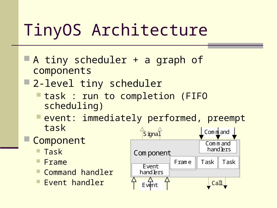
TinyOS Architecture
A tiny scheduler + a graph of components 2-level tiny scheduler
task : run to completion (FIFO scheduling) event: immediately performed, preempt task
Component Task Frame Command handler Event handler
Command
Component
Event
Signal
Task
Command handlers
Event handlers
Frame Task
Call

TinyOS-nesC System programming language [Gay03]
To support TinyOS programming model Component specification
provides and uses interfaces interface contains commands and events
Component implementation Module : provide code and implement interfaces Configuration : connect uses-interface of component to provides-
interface of other component Support for concurrency
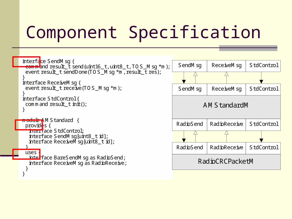
interf ace SendMsg { command result_t send(uint16_t, uint8_t, TOS_Msg *m); event result_ t sendDone(TOS_Msg *m, result_ t res);}interf ace ReceiveMsg { event result_ t receive(TOS_Msg *m);}interf ace StdControl { command result_t init();}
module AMStandard { provides { interf ace StdControl; interf ace SendMsg[uint8_t id]; interf ace ReceiveMsg[uint8_t id]; } uses { interf ace BareSendMsg as RadioSend; interf ace ReceiveMsg as RadioReceive; }}
AMStandardM
SendMsg ReceiveMsg StdControl
RadioSend RadioReceive StdControl
SendMsg ReceiveMsg StdControl
RadioCRCPacketM
RadioSend RadioReceive StdControl
Component Specification

Component Implementation
module AMstandard { .... }
I mplement { bool state; TOS_Msg* buff er;
command result_ t SendMsg.send[uint8_t id](uint16_t addr,uint8_t length, TOS_Msg* data) { .... post sendTask(); buff er = data; .... } event result_ t RadioSend.sendDone(TOS_Msg* msg, result_ t res) { .... signal SendMsg.sendDone[msg->type](msg, success); .... } event TOS_MsgPtr RadioReceive.receive(TOS_Msg* packet) { .... signal ReceiveMsg.receive[packet->type](packet); .... } task void sendTask() { ..... call RadioSend.send(buff er); .... }
confi guration GenericComm { .... }
implementation{ components AMStandard; components RadioCRCPacket as RadioPacket; components UARTFramedPacket as UARTPacket;
Control = AMStandard.Control; SendMsg = AMStandard.SendMsg; ReceiveMsg = AMStandard.ReceiveMsg; sendDone = AMStandard.sendDone;
AMStandard.UARTControl -> UARTPacket.Control; AMStandard.UARTSend -> UARTPacket.Send; AMStandard.UARTReceive -> UARTPacket.Receive;
AMStandard.RadioControl -> RadioPacket.Control; AMStandard.RadioSend -> RadioPacket.Send; AMStandard.RadioReceive -> RadioPacket.Receive;}
Code Wiring

A TinyOS application: DIM
DI M
GPSR Timer
Clock
HPLClock
Clocks
Temperature
ADC
HPLADC
I 2C
AM
RadioCRCPacket
CC1000RadioI nt
CC1000
UARTFramPacket
UART
UART
SW
HW
application
routing
message
packet
byte

Common System Components
AM (Active Message) Messaging layer
implementation that for packet de-muxing
RadioCRCPacket Provides simple radio
abstraction Send/receive packets
over radio
RadioCRCPacket
CC1000RadioI nt
RadioCRCPacket
MicaHighSpeedRadio
Mica2Radio(76.8 KBaud)
MicaRadio(40Kbps)

Common System Components UARTFramedPacket
provides serial communication to Host PC 19.2kbps(Mica/Mica2Dot), 57.6Kbps(mica2)
Timer provides periodic and one-shot timers
ADC abstraction of the analog-to-digital converter used by sensing components
Temperature, light sensor

Components of Infrastructure
Processor Platforms Radios Sensors
Operating Systems
Localization Time Synchronization Medium Access Calibration
Collaborative Signal Processing
Data-centric Routing Data-centric Storage
Querying, Triggering
Aggregation and Compression
Collaborative Event Processing
Mon
itor
ing

MAC Layer Issues
Energy-efficient MAC layers Topology control for higher energy-efficiency MAC and radio layer performance

Medium Access Control
Important design considerations Collision avoidance Energy efficiency Scalability in node density Latency Fairness Throughput Bandwidth utilization
Reduce idle listening, collisions, control overhead, overhearing

MAC Design in TinyOS
CSMA/Collision Avoidance Optional MAC layer acknowledgement (Mica) Hill et al. 2002
Synchronization
Start Symbol Search Receiving individual bits
StartSym Detection
RX
MAC Delay Transmitting encoded bits
TX
Ack
StartSym

Sensor-MAC (S-MAC)
Tradeoffs Higher latency, less fairness Higher energy efficiency
Major components in S-MAC Periodic listen and sleep Collision avoidance Overhearing avoidance Message passing
Combine TDMA and contention-based protocols
Ye et al., Infocom2002
Latency
Fairness Energy

Collision Avoidance
Solution: Similar to IEEE 802.11 ad hoc mode (DCF) Physical and virtual carrier sense Randomized backoff time RTS/CTS for hidden terminal problem RTS/CTS/DATA/ACK sequence
Overhearing avoidance Reserve channel for duration of entire message (rather than a
fragment) … so that others can aggressively sleep to avoid overhearing
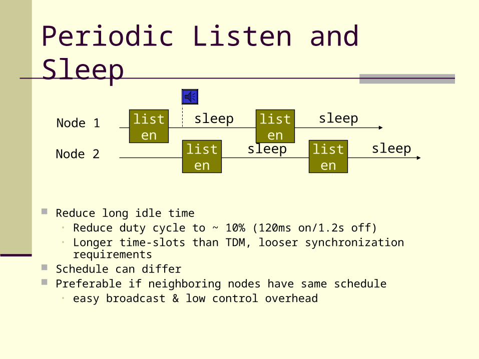
Periodic Listen and Sleep
Reduce long idle time • Reduce duty cycle to ~ 10% (120ms on/1.2s off) • Longer time-slots than TDM, looser synchronization requirements
Schedule can differ Preferable if neighboring nodes have same schedule
• easy broadcast & low control overhead
Node 1 sleeplisten listen sleep
Node 2 sleeplisten listen sleep

Schedule 2
Coordinated Sleep
Nodes coordinate on sleep schedules Nodes periodically broadcast schedules New node tries to follow an existing schedule Nodes on border of two schedules follow both
Periodic neighbor discovery and synchronization Early part of listen interval devoted to this
Schedule 1 1
2

Implementation on Testbed
Platform Mica/Mica2 Motes TinyOS Used as NIC for x86/xscale embedded Linux box
Configurable S-MAC options Low duty cycle with
adaptive listen Low duty cycle without
adaptive listen Fully active mode (no
periodic sleeping)
S-MAC Performance
Two-hop network at different traffic loads
S-MAC consumes much less energy than 802.11-like protocol w/o sleeping
At heavy load, overhearing avoidance is the major factor in energy savings
At light load, periodic sleeping plays the key role
Source 1
Source 2
Sink 1
Sink 2
0
2
4
6
8
10
200
400
600
800
1000
1200
1400
1600
1800 Average energy consumption in the source nodes
Message inter-arrival period (second)
Ene
rgy
cons
umpt
ion
(mJ)
802.11-like protocol without sleep
Overhearing
avoidance
S-MAC

Adaptive Topology Control
Can we put nodes to sleep for long periods of time?
More aggressively than S-MAC Leverage redundant deployments
Topology adapts to Application activities Environmental changes Node density
Extend system lifetime Reduce traffic collision Complementary to topology control
schemes that adjust transmit power levels

Example: ASCENT
The nodes can be in active or passive state Active nodes forward data packets (using a routing
mechanism that runs on the topology). Passive nodes do not forward packets but might sleep or
collect network measurements. Each node joins the network topology or sleeps according to
the number of neighbors and packet loss as measured locally.

ASCENT State Transitions
Test
Passive Sleep
Active
after Tt
after Tp
after Ts
neighbors < NT and • loss > LT • loss < LT & help
neighbors > NT (high ID for ties); or loss > loss T0
NT: neighbor threshold
LT: loss threshold
T?: state timer values (p: passive, s: sleep, t: test)

Topology Control Schemes
Empirical adaptation: Each node adapts based on measured operating region. ASCENT (Cerpa et al. 2002)
Routing/Geographic topology based: Redundant links are removed. SPAN (Chen et al. 2001), GAF (Xu et al. 2001)
Cluster based: Workload is shared within clusters CEC (Xu et al. 2002)
Data/traffic driven: Nodes starts on demand using paging channel STEM (Tsiatsis et al. 2002)
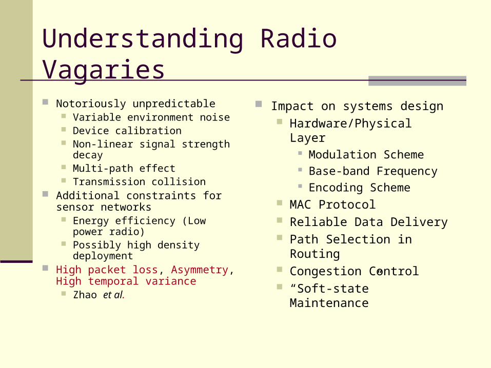
Understanding Radio Vagaries
Notoriously unpredictable Variable environment noise Device calibration Non-linear signal strength decay Multi-path effect Transmission collision
Additional constraints for sensor networks Energy efficiency (Low power
radio) Possibly high density
deployment High packet loss, Asymmetry,
High temporal variance Zhao et al.
Impact on systems design Hardware/Physical Layer
Modulation Scheme Base-band Frequency Encoding Scheme
MAC Protocol Reliable Data Delivery Path Selection in Routing Congestion Control “Soft-state” Maintenance

Spatial Profile of Packet Delivery
Node positions
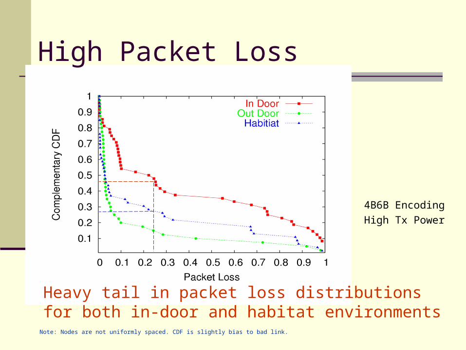
4B6B Encoding
High Tx Power
In-door
2hrs (7200 pkts)
“Gray Area” is evident in the communication range

Grey Area in Packet Loss Relatively large region of
poor connectivity Across a wide variety of
environments Spanning as large as 30%
of the effective transmission range
In-door
Out-door Unobstructed
4B6B Encoding
High Tx Power
High Packet Loss
Note: Nodes are not uniformly spaced. CDF is slightly bias to bad link.
Heavy tail in packet loss distributions for both in-door and habitat environments

Standard Deviation in Packet Loss
Window size = 40
4B6B Encoding
High Tx Power
Variability over time with large dynamic range

Components of Infrastructure
Processor Platforms Radios Sensors
Operating Systems
Localization Time Synchronization Medium Access Calibration
Collaborative Signal Processing
Data-centric Routing Data-centric Storage
Querying, Triggering
Aggregation and Compression
Collaborative Event Processing
Mon
itor
ing

What is localization?
Determining the location of a node in a global coordinate system
Availability of location information is a fundamental need Interpreting the data Routing (GPSR) Geo-spatial queries Location based addressing
Why not equip every node with GPS? GPS needs line of sight, cannot be used
in indoor environments in the presence of foliage
Early Schemes
Active Bat (AT&T) People wear badges which emit ultra-sound pulse Receivers mounted in a regular grid on ceiling Time of flight based triangulation (centralized)
CRICKET (MIT) Ultrasound ranging Fixed emitter infrastructure with known positions
RADAR (Microsoft Research) Uses existing 802.11 LAN Signal/Noise ratio of the targets used for localization

Ad-hoc Localization
Sensor nodes are randomly scattered
“Where am I”? Only a “small” fraction of
nodes have GPS Anchors
The rest have to infer their global positions somehow

General Approach
Find distance to neighboring nodes Ranging
Neighbors of anchors fix position relative to anchors Position fixing
Other nodes fix their positions relative to at least three neighbors
Iterative refinement

Ranging
Radio Received signal strength based Use a path loss model to estimate range Need careful calibration for accuracy
Can get to within 10% of radio range Examples: SpotON (Hightower et al.), Calamari (Whitehouse et al.)
Acoustic Use time of flight of sound (ultrasound) Potentially high accuracy: 1% of radio range May need code spreading to counter multipath effects Examples: Girod et al., Savvides et al.

•
Position Fixing Taxonomy
Topological Schemes Rely only on topology information Can result in very inaccurate localization Usually require less resources
Geometric Schemes Use geometric techniques to determine location Usually result in highly accurate position estimates May require more resources

d1
d2
d3
d1+d2+d3
Topological Schemes
DV-Hop (Niculescu et. al.) Find average distance or hop
davg distance = davg*(No of Hops) requires no ranging!!!
DV-Dist (Niculescu et. al.) Standard distance vector
algorithm range as metric
Refinement can help significantly

x
y
Geometric Schemes
Savvides et. al. Each anchor defines a
coordinate system, anchor is the origin.
nodes localize in this coordinate system using hop by hop lateration
nodes maintain (nodeId, x,y) 3 such tuples can be used to
localize Observations
Local coordinates may be translated, rotated or flipped versions of the global system
distance from anchor is invariant

Comparison of existing schemes
3 schemes (20% anchors, 1% error) Geometric (Savvides et al.,
Niculescu et. al.) Topological (DV-dist)
Localization extent Nodes localized within 2m
Topological scheme Higher localization extent
than geometric scheme. Need 10-11 neighbors

The State of Localization
Lots of research in the area Probably far from deploying robust systems in the
field Every component is hard and error-prone
Ranging Position-fixing

Components of Infrastructure
Processor Platforms Radios Sensors
Operating Systems
Localization Time Synchronization Medium Access Calibration
Collaborative Signal Processing
Data-centric Routing Data-centric Storage
Querying, Triggering
Aggregation and Compression
Collaborative Event Processing
Mon
itor
ing

Time Synchronization
Critical piece of functionality Applications:
Sample-level correlation Event time correlations
Wide variety of requirements Microsecond level for acoustic
localization Perhaps less for events Global? Post-facto?
Prior work NTP
Research Systems
RBS (Elson et al.) TPSN (Ganeriwal et al.) DMTS (Ping Su) LTS (van Greunen et al.)
Theory Optimal global
synchronization (Karp et al. and Hu et al.)

One-Hop Synchronization
Key step: determine clock offset
Observation: Can use timestamped message exchange to infer clock offset Similar to the NTP
algorithm Tricky
1T
2T 3T
4T
))()((5.0 3412 TTTToffset

Timing Components
Send Processing Time
Access Time
Propagation Latency
Transmission Latency
Receive Processing
Time
Non-Deterministic
Negligible
Deterministic
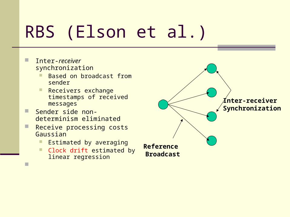
RBS (Elson et al.)
Inter-receiver synchronization Based on broadcast from sender Receivers exchange timestamps of
received messages Sender side non-determinism eliminated Receive processing costs Gaussian
Estimated by averaging Clock drift estimated by linear
regression
Reference Broadcast
Inter-receiver Synchronization
TPSN and LTS
Sender-side synchronization Use the NTP algorithm TPSN
Timestamps packets as close to radio as possible to remove non-determinism
LTS Uses RBS-style averaging
to remove non-determinism
1T
2T 3T
4T
))()((5.0 3412 TTTToffset

DMTS One-way, one-packet synchronization Receiver computes offset from sender’s clock
Do away with all sources of non-determinism by timestamping close to radio layer
Send Processing Time
Access Time
Propagation Latency
Transmission Latency
Receive Processing
Time
Non-Deterministic
Negligible
Deterministic
TimestampTimestamp

Multihop Synchronization
Goals Synchronize a pair of nodes
across multiple hops Synchronize all nodes with
a base-station Basic idea is the same in both
cases Successively synchronize
nodes along a path In the latter case, do it over
a spanning tree Error accumulates linearly
Reducing the Error
One-hop synchronization estimates offsets between nodes For global synchronization, need:
Minimum variance offset estimation Consistent maximum likelihood estimation of clock values
Theoretical result: There exists estimators that jointly determine minimum variance offsets that give maximum likelihood times Karp et al. and Hu et al.
Both based on the observation that one can use information along multiple paths
Error grows logarithmically

Components of Infrastructure
Processor Platforms Radios Sensors
Operating Systems
Localization Time Synchronization Medium Access Calibration
Collaborative Signal Processing
Data-centric Routing Data-centric Storage
Querying, Triggering
Aggregation and Compression
Collaborative Event Processing
Mon
itor
ing