Sensors 2014, 14, 2199-2224; doi:10.3390/s140202199OPEN ACCESS

sensorsISSN 1424-8220

www.mdpi.com/journal/sensors

Article

A Multimetric, Map-Aware Routing Protocol for VANETs inUrban AreasCarolina Tripp-Barba 1,2,*, Luis Urquiza-Aguiar 1, Monica Aguilar Igartua 1,David Rebollo-Monedero 1, Luis J. de la Cruz Llopis 1, Ahmad Mohamad Mezher 1

and Jose Alfonso Aguilar-Calderon 2

1 Department of Telematic Engineering, Universitat Politecnica de Catalunya (UPC),C/ Jordi Girona 1-3, Barcelona 08034, Spain; E-Mails: luis.urquiza@entel.upc.edu (L.U.-A.);maguilar@entel.upc.edu (M.A.I.); david.rebollo@entel.upc.edu (D.R.-M.);luis.delacruz@entel.upc.edu (L.J.C.L.); ahmad.mezher@entel.upc.edu (A.M.M.)

2 Faculty of Informatics, Autonomic University of Sinaloa (UAS), De los Deportes Avenue andLeonismo Internacional s/n, Mazatlan 82107, Mexico; E-Mail: ja.aguilar@uas.edu.mx

* Author to whom correspondence should be addressed; E-Mail: ctripp@maz.uasnet.mx;Tel.: +52-1-6691-20-23-83.

Received: 3 December 2013; in revised form: 4 January 2014 / Accepted: 8 January 2014 /Published: 28 January 2014

Abstract: In recent years, the general interest in routing for vehicular ad hoc networks(VANETs) has increased notably. Many proposals have been presented to improve thebehavior of the routing decisions in these very changeable networks. In this paper, wepropose a new routing protocol for VANETs that uses four different metrics. which arethe distance to destination, the vehicles’ density, the vehicles’ trajectory and the availablebandwidth, making use of the information retrieved by the sensors of the vehicle, in order tomake forwarding decisions, minimizing packet losses and packet delay. Through simulation,we compare our proposal to other protocols, such as AODV (Ad hoc On-Demand DistanceVector), GPSR (Greedy Perimeter Stateless Routing), I-GPSR (Improvement GPSR) andto our previous proposal, GBSR-B (Greedy Buffer Stateless Routing Building-aware).Besides, we present a performance evaluation of the individual importance of each metricto make forwarding decisions. Experimental results show that our proposed forwardingdecision outperforms existing solutions in terms of packet delivery.

Sensors 2014, 14 2200

Keywords: vehicular ad hoc networks; multi-metric forwarding decisions; geographicrouting protocol

1. Introduction

Vehicular ad hoc networks (VANETs) [1,2] are an emerging area of wireless networking thatfacilitate ubiquitous connectivity among smart vehicles through vehicle-to-vehicle (V2V) communicationsand between vehicles and the city or the road infrastructure through vehicle-to-roadside (V2R)communications. This emerging technology field aims to improve the safety of passengers, alleviate thetraffic flow, reduce pollution and enable in-vehicle entertainment applications for passengers. Safetyapplications can reduce accidents by providing traffic information to drivers, such as collision warning,road surface conditions or the state of the traffic flow. Moreover, passengers could use the availableinfrastructure of the city to connect to the Internet for entertainment applications [3].

The growing interest in this technology is an incentive for car manufacturers, the research communityand governments who, day after day, increase their efforts towards creating a standardized platformfor vehicular communications. The unique characteristics and some special requirements of VANETsgenerate different challenges for the research community. To address these challenges in both safetyand comfort-oriented applications, there is a pressing need to develop new routing protocols speciallydesigned for this kind of network, which provide a good performance, either under sparse or dense trafficconditions. This work proposes a new routing protocol for VANETs, which considers several metricsto select the best next forwarding node for each packet in each step towards its destination. Simulationresults show the benefits of our protocol compared to other proposals under different network conditions.

2. Related Work

Traditional traffic management systems are based on centralized infrastructures in which camerasand sensors placed along the roadside collect information about vehicle density and the traffic state.These data are sent to a central unit that processes them and makes appropriate decisions. This typeof framework is very costly in terms of deployment and is characterized by the long time needed toprocess information.

The rapid development of wireless communication has raised the interest for car manufacturers,the research community and governments, making a new decentralized architecture based onvehicle-to-vehicle communications. Vehicular ad hoc networks are a specific type of mobile ad hocnetwork (MANET) [1] in which the nodes are vehicles. The road-constrained characteristics of thesenetworks, the high mobility of the vehicles, their unbounded power source and the presence of roadsidewireless infrastructures make VANETs an important research topic. The main purpose of VANETs is tobe a platform that can support intelligent inter-vehicle communication, improving traffic safety, althoughthey are also useful for traffic management and other services, e.g., Internet access.

The presence of city infrastructure in emerging smart cities has an important impact on urbancommunications. In some applications, one must find a route to the closest access point (AP), e.g.,

Sensors 2014, 14 2201

connecting to the Internet. In a city with advanced wireless infrastructure deployed, it would take only afew hops to reach the nearest AP under day-traffic conditions. Roadside access points should be placedin special locations, such as on traffic lights, since they are well positioned to act as traffic routers. Theyalready form a traffic grid, usually located where traffic is most intense, and are equipped with a powersupply and directly maintained by local municipalities. For instance, [4] proposes a priority intersectioncontrol scheme in a self-organized manner, so that smart traffic lights detect the presence of emergencyvehicles and assign them a priority at intersections. The goal is to provide a “green-wave” signal displayfor the emergency vehicles seeking to avoid accidents.

Several proposals of routing protocols for VANETs have been presented. Research works claim thatthe best routing protocols for VANETs are those that use geographic routing, which are based on theknowledge of the instantaneous locations of nodes [5].

GPSR (greedy perimeter stateless routing) [6] is a well-known geographic routing protocol speciallydesigned for VANETs. It forwards packets to the neighbor node that is closest to destination following ahop-by-hop scheme. GPSR uses two different techniques to forward packets: greedy forwarding, whichis used by default, and perimeter forwarding, which is used whenever greedy forwarding cannot beused. Since nodes require knowing their neighbors’ positions, they periodically transmit a hello messagecontaining their own identifier (e.g., IP address) and their position. Several proposals that improveGPSR have been presented in the literature. The authors in [7] proposed movement prediction-basedrouting (MOPR), which improves the routing process of GPSR by selecting the most stable route interms of lifetime with respect to the movement of vehicles. In [8], an algorithm was proposed thatmodifies GPSR and exploits information about movement to improve the next forwarding node decision.The authors use information about position, moving direction and speed to make routing decisions.The proposed protocol was compared to GPSR in a highway setting, showing improvement. AdvancedGreedy Forwarding (AGF) [9] improves the performance of GPSR, since its forwarding technique ismore fault-tolerant than the traditional greedy forwarding.

Recently, some proposals of routing protocols for VANETs that include several metrics have beenpresented. The use of alternative metrics in VANETs in addition to the classic distance has shown notablebenefits. For instance, the trajectory of the vehicles is used in [7,10]. The authors in [11] propose theImprovement GPSR routing protocol (I-GPSR), which incorporates distance, vehicle density, movingdirection and vehicle speed to make packet forwarding decisions. A new data forwarding mechanism,which uses a store-carry-forward scheme besides the position information and moving direction of thenodes, was presented in [10].

Nevertheless, none of the existent proposals takes the available bandwidth into account as a metric tomake forwarding decisions. The reason could be that obtaining a fairly simple, but accurate, model tocalculate the available bandwidth in VANETs is a difficult task. Our proposal includes several metricsto optimize the selection of the next forwarding node in a geographic-based protocol. These metricsare vehicle density, trajectory, distance to destination and available bandwidth. The trajectory of a nodeconsists of its moving direction and speed, which are used to estimate how fast a node gets near toor goes away from a destination. Then, we weight those four metrics into a single multimetric score.Furthermore, we evaluate the performance of each single metric compared to the global multimetricvalue and also to some combination of them.

Sensors 2014, 14 2202

3. Multimetric Map-Aware Routing Protocol (MMMR)

3.1. Motivation

VANET nodes are vehicles that move along roads, potentially at a high speed. These vehiclesfollow transit rules, respect the direction of the streets, traffic lights and also the presence of buildingsand other vehicles. The vehicle density in VANETs constantly changes depending on the area andthe time of the day, so it is difficult to establish and maintain end-to-end communication pathsbetween sources and destinations, as is traditionally done in MANETs. Several routing protocols basedon geographic information have specially been proposed for VANETs. Nonetheless, a proper dataforwarding mechanism is still needed to cope with the special constraints of VANETs, e.g., the highnodes’ speed, the dynamic network topology and the variable nodes’ density.

We propose a new routing protocol for VANETs in urban scenarios that we call the multimetricmap-aware routing protocol (MMMR). MMMR seeks to improve the decision of the next forwardingnode based on four routing metrics, which are the distance to destination, the vehicles’ density, thevehicles’ trajectory and the available bandwidth. We weight the four metrics to finally obtain amultimetric value for every neighbor node that is a candidate as the next forwarding node. The schemeis self-configured and able to adapt to the changing vehicles’ density in real time.

In our proposal, we can distinguish five processes: map-aware capability, use of a local buffer,signaling, the evaluation of metrics and the forwarding decision. We explain each one in the following.

3.2. Map-Aware Capability and Use of a Local Buffer

An important issue that one should face in the design of a routing protocol for VANETs in urbanscenarios is the presence of the buildings, trees and other obstacles usually found in cities. Greedyforwarding in GPSR is often restricted,because direct communication between nodes may not exist, dueto an obstacle. We include a map-aware capability, which focuses on two important enhancements: (a) ittakes into account the presence of buildings in the decision of the next forwarding node; and (b) it usesa local buffer to temporarily store packets when no forwarding node was found.

The forwarding decision included in MMMR uses the same criteria as the original GPSR [6]. Itconsists in choosing the neighbor located nearest to a destination. Besides, our proposal tackles theimportant issue of deciding which neighbors are actually reachable. This feature is of paramountimportance to determine if a neighbor in the list could be a good forwarding node. The accurateinformation about the current position of a neighbor has a strong impact on the routing performance,because knowing this information makes the node aware of which neighbors are reliable to act as thenext forwarding nodes. At the same time, it avoids sending packets to an unreachable node, becauseit is, for instance, behind a building. This feature makes vehicles be map-aware, since they avoidsending packets to nodes behind the walls of the buildings in the city. The presence of obstacles, such asbuildings, are tackled using vehicular location. If the straight line between the current vehicle positionand the next vehicle position is blocked by any rectangular area representing a building, then that nodebehind a building cannot be chosen as the next forwarding node. Otherwise, packets sent to that nodewould be lost.

Sensors 2014, 14 2203

Furthermore, an important drawback of GPSR is the implementation of perimeter forwarding,because it is not clear when the algorithm switches its mode to greedy forwarding again. The mainproblem of GPSR is the use of outdated information to select the next forwarding node. It is possibleto find inconsistencies in the neighbor tables or in destination node’s location set in the packet. Theneighbor table problem is to select a node that is out of range, resulting in packet loss. This happenoften because often, the nearest neighbor to the destination node is also the farthest neighbor. Due todestination node’s location included in the packet, the header is never updated by any forwarding node;packets with high a delay will never arrive to the destination node and will get lost in a location wherethe destination is no longer. In addition, mobility can induce routing loops while using the perimetermode [12]. To avoid these problems caused by perimeter forwarding, our proposal stores packets in alocal buffer of the current relaying node when there is no neighbor that satisfies all the requirementsneeded to be a next forwarding node. If at least one of the two conditions (i.e., being actually areachable neighbor and being closer than the current carrier node to the destination) required to bethe next forwarding node is not satisfied, then packets are stored according to the FCFS (First-Come,First-Served) scheme in a local buffer instead of being discarded. If the buffer gets full, packets willbe dropped. The nodes periodically look for a neighbor that can satisfy the requirements to be the nextforwarding node. Every period of time (1 s), the node looks for a new node candidate. After previoussimulations analysis, it was concluded that this period of time is frequent enough to detect quickly anytopology change. If a candidate fulfills the requirements, the stored packets are forwarded to that node.In our case, the impact of out of order is not remarkable, due to the kind of services that we use, such asthe report of accidents, traffic or environmental information obtained by the car sensors.

We use the LOS (line of sight) criteria, because our evaluation scenario is a city, i.e., an urban zonewith walls and buildings. Besides, the evaluated network is a VANET (nodes are vehicles). Thus, inthis case, the more important and restrictive point to take into account is the line of sight of the nodes inthe network. Due to that, in the moment the forwarding decision is made, we act in a conservative way,considering only as candidates to be the next forwarding node those nodes that actually can receive thepacket, because they are in the LOS of the current carrying node.

Concluding, three conditions must be verified for a node to be chosen as the next forwarding node,i.e., being in the coverage range, in LOS (line of sight) and nearer to a destination than the current node.If the candidate fulfills all three requirements, packets are forwarded to it; otherwise, packets are storedin the local buffer of the current carrier node.

In addition to these two improvements, the decision of the next forwarding node is based on thecombination of four metrics, which are detailed in Section 3.4.

3.3. Signaling

MMMR, as most geographic routing protocols, requires nodes to periodically send signalingmessages announcing their presence to the neighbors in transmission range. To obtain precise locationinformation about each node without introducing new signaling messages, we use a new format of theexisting hello messages (HM) to exchange information between neighbors. The format of hello messagesused by MMMR is presented in Table 1, and they include the following fields:

Sensors 2014, 14 2204

• ID: A four-byte field with the identifier of each node.• Position: This field is divided into 32 bits for latitude (lx) and 32 bits for longitude (ly), which

represent the geographic position of each node. Each set of 32 bits is also divided into one bit forthe direction (north or south for longitude; east or west for latitude), eight bits for the grades, sixbits for the minutes and 17 bits for the seconds.• Velocity: A two-byte field that uses one byte for speed (m/s) in the x-axis (vx) and one byte for

speed in the y-axis (vy). Each node calculates its own speed from two consecutive position points,(x1, y1) and (x2, y2), taken at times t1 and t2:

vx =x2 − x1t2 − t1

, vy =y2 − y1t2 − t1

(1)

• Antenna sensing (S): One byte to express the antenna sensing in the power ratio in decibels(dBm) used by the node. A signal power below the antenna sensing is not detectable.• Idle time (tidle): Each node calculates the units of time that it spends without sending nor receiving

data since the last HM sent. This value is represented in one byte. That is, tidle measures the amountof time the node is idle between two consecutive hello messages.• Density (ρ): One byte to represent the number of neighbors within the transmission range at the

moment of sending the current hello message.

Table 1. Hello messages (HMs) format in the multimetric map-aware routing protocol.

ID lx ly vx vy S tidle ρ

32 bits 32 bits 32 bits 8 bits 8 bits 16 bits 8 bits 8 bits

When a node receives a hello message from a neighbor in transmission range, the node stores thereception time and updates its neighbor list with all the values shown in Table 1. This is done followingthe conditions shown in Algorithm 1. If a hello message is received from a neighbor already registeredin the neighbor list, the information of this neighbor is just updated (Lines 1, 2 from Algorithm 1). Tokeep the list of neighbors updated and to use only nodes that actually are in transmission range, nodesremain in a neighbors list for twice the interval between consecutive hello messages.

In addition, we were careful to check whether a node was located too close to the transmissionrange before considering it as a neighbor. When a node receives a hello message from a new neighbor(a neighbor not yet registered in the list), it has first to check if this is a stable node before adding it in theneighbor list. This means that hello messages have to be received with a power higher than the antennasensing plus a security margin (Lines 4 to 8). We set this security margin to 1 dB, since we observedfrom simulation results that this was a proper value. If this condition is not fulfilled, that neighbor willnot be included in the neighbor list (Line 7), since this node probably is around the border line of thetransmission range.

Sensors 2014, 14 2205

Algorithm 1 Updating the neighbor list.Require: A new hello message received with these parameters: ID, lx, ly, vx, vy, S, tidle, ρ.

1: if (The neighbor is already in the neighbor list) then2: Update neighbor information3: else4: if (Reception power ≥ antenna sensing + 1 dB) then5: Add node in the neighbor list6: else7: Ignore hello message8: end if9: end if

The sending period of hello messages could be higher to obtain more accuracy in the composition ofthe list of neighbors, although a higher signaling traffic could produce an increase in packet collisions.By default, the sending period of the HM is set to 1 s.

The list of neighbors includes the data sent in hello messages (see Table 1) and the data shown inTable 2. For each neighbor, i, we store the reception time when the last hello message arrived (thereception time of the last HM in Table 2). This is done to estimate the future position of that neighbornode. Furthermore, we store the moment when the first hello message arrived (the reception time ofthe first HM )and the total number of hello messages received (No. HM). These values will be used toestimate the available bandwidth using a metric explained in the next section.

Table 2. Extra data per node used in the neighbor list included in the HM.

Neighbor i Reception Time of the Last HM Reception Time of the First HM No. HM

32 bits 8 bits 8 bits 8 bits

3.4. Metrics Evaluation

In this section, we detail each one of the four metrics included in our multimetric algorithm MMMR,which is a geographic routing protocol based on hop-by-hop forwarding decisions. The use of thesemetrics is a way to improve the choice of the next forwarding node. The four metrics considered are thedistance to a destination, the trajectory of the vehicles, the nodes’ density and the available bandwidth.They are described below.

Distance: The typical goal of most geographic routing protocols is to send packets hop-by-hop totheir destination, so that the next forwarding hop is the neighbor that is closest to the destination. Thesekind of protocols are based on the knowledge of geographic information of every node in the scenario.Each vehicle knows its own position and also the position of the destination. Therefore, it is usuallyassumed that the position of the packet’s destination and the positions of the next hop candidates aresufficient to make proper forwarding decisions. We also use the distance (d) to the destination as ametric to evaluate each neighbor in our proposal. We obtain this information from the fact that senders

Sensors 2014, 14 2206

know the destination position (xD, yD) and also each neighbor includes in the hello messages its ownposition. With the position (xi, yi) of each neighbor, i, we can obtain its Euclidean distance (di) to thedestination (D) (see Equation (2)):

di((xi, yi), (xD, yD)) = ‖~xi − ~xD‖ =√

(xi − xD)2 + (yi − yD)2 (2)

To compute the metric based on this distance, u1,i, we use Expression (3), where di is the previousEuclidean distance and dref is a reference distance, above which losses start to increase notably faster.This dref is obtained from simulations where we evaluated the performance of a fixed node set in differentdistances from the AP. The results are presented in Figure 1, where we can see that dref is around 2,000 min our urban scenario. Notice that for a transmission range of 250 m, such a path of around 2,000 mwould take around eight hops. α is an attenuation factor that equals 0.77, obtained after a mathematicalregression using the results of the simulations mentioned before and shown in Figure 1. This value,represented in Figure 1, measures the utility of the metric of the distance. Consequently, low distancesto the destination obtain a high benefit, while long distances to the destination obtain low profits. Themain settings used in this evaluation are presented in Table 3.

Figure 1. The relation between the distance to the destination and packet losses.

Table 3. The main simulation setting used in the distance evaluation.

Parameter Value

Simulation area 1,500 m × 1,500 mNumber of nodes 120 vehiclesMaximum node speed 50 km/hTransmission/sensing range 250/300 mMAC specification IEEE 802.11pQoS access category BE (best effort)Bandwidth 12 MbpsSimulation time 1,000 sMaximum packet size 1,000 bytesTraffic profile CBR (Constant Bit Rate) 4 KbpsRouting protocol GPSR

Sensors 2014, 14 2207

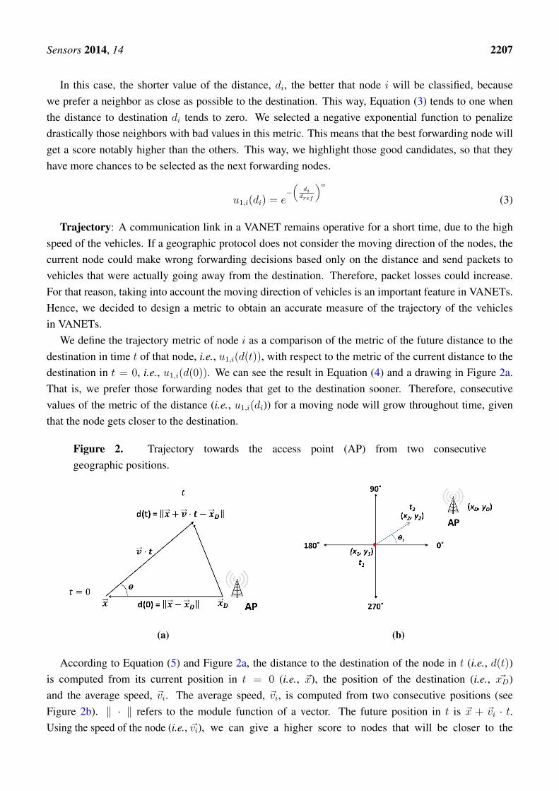
In this case, the shorter value of the distance, di, the better that node i will be classified, becausewe prefer a neighbor as close as possible to the destination. This way, Equation (3) tends to one whenthe distance to destination di tends to zero. We selected a negative exponential function to penalizedrastically those neighbors with bad values in this metric. This means that the best forwarding node willget a score notably higher than the others. This way, we highlight those good candidates, so that theyhave more chances to be selected as the next forwarding nodes.

u1,i(di) = e−(

didref

)α(3)

Trajectory: A communication link in a VANET remains operative for a short time, due to the highspeed of the vehicles. If a geographic protocol does not consider the moving direction of the nodes, thecurrent node could make wrong forwarding decisions based only on the distance and send packets tovehicles that were actually going away from the destination. Therefore, packet losses could increase.For that reason, taking into account the moving direction of vehicles is an important feature in VANETs.Hence, we decided to design a metric to obtain an accurate measure of the trajectory of the vehiclesin VANETs.

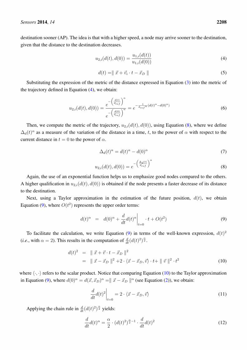
We define the trajectory metric of node i as a comparison of the metric of the future distance to thedestination in time t of that node, i.e., u1,i(d(t)), with respect to the metric of the current distance to thedestination in t = 0, i.e., u1,i(d(0)). We can see the result in Equation (4) and a drawing in Figure 2a.That is, we prefer those forwarding nodes that get to the destination sooner. Therefore, consecutivevalues of the metric of the distance (i.e., u1,i(di)) for a moving node will grow throughout time, giventhat the node gets closer to the destination.

Figure 2. Trajectory towards the access point (AP) from two consecutivegeographic positions.

(a) (b)

According to Equation (5) and Figure 2a, the distance to the destination of the node in t (i.e., d(t))is computed from its current position in t = 0 (i.e., ~x), the position of the destination (i.e., ~xD)and the average speed, ~vi. The average speed, ~vi, is computed from two consecutive positions (seeFigure 2b). ‖ · ‖ refers to the module function of a vector. The future position in t is ~x + ~vi · t.Using the speed of the node (i.e., ~vi), we can give a higher score to nodes that will be closer to the

Sensors 2014, 14 2208

destination sooner (AP). The idea is that with a higher speed, a node may arrive sooner to the destination,given that the distance to the destination decreases.

u2,i(d(t), d(0)) =u1,i(d(t))

u1,i(d(0))(4)

d(t) =‖ ~x+ ~vi · t− ~xD ‖ (5)

Substituting the expression of the metric of the distance expressed in Equation (3) into the metric ofthe trajectory defined in Equation (4), we obtain:

u2,i(d(t), d(0)) =e−(d(t)dref

)α

e−(d(0)dref

)α = e− 1dref

α (d(t)α−d(0)α)(6)

Then, we compute the metric of the trajectory, u2,i(d(t), d(0)), using Equation (8), where we define∆d(t)

α as a measure of the variation of the distance in a time, t, to the power of α with respect to thecurrent distance in t = 0 to the power of α.

∆d(t)α = d(t)α − d(0)α (7)

u2,i(d(t), d(0)) = e−(

∆d(t)

dref

)α(8)

Again, the use of an exponential function helps us to emphasize good nodes compared to the others.A higher qualification in u2,i(d(t), d(0)) is obtained if the node presents a faster decrease of its distanceto the destination.

Next, using a Taylor approximation in the estimation of the future position, d(t), we obtainEquation (9), where O(t2) represents the upper order terms:

d(t)α = d(0)α +d

dtd(t)α

∣∣∣∣t=0

· t+O(t2) (9)

To facilitate the calculation, we write Equation (9) in terms of the well-known expression, d(t)2

(i.e., with α = 2). This results in the computation of ddt

(d(t)2)α2 .

d(t)2 = ‖ ~x+ ~v · t− ~xD ‖2

= ‖ ~x− ~xD ‖2 +2 · 〈~x− ~xD, ~v〉 · t+ ‖ ~v ‖2 · t2 (10)

where 〈·, ·〉 refers to the scalar product. Notice that comparing Equation (10) to the Taylor approximationin Equation (9), where d(0)α = d(~x, ~xD)α =‖ ~x− ~xD ‖α (see Equation (2)), we obtain:

d

dtd(t)2

∣∣∣∣t=0

= 2 · 〈~x− ~xD, ~v〉 (11)

Applying the chain rule in ddt

(d(t)2)α2 yields:

d

dtd(t)α =

α

2· (d(t)2)

α2−1 · d

dtd(t)2 (12)

Sensors 2014, 14 2209

At t = 0, we have d(0) = d and ddtd(t)2

∣∣t=0

= 2 · 〈~x− ~xD, ~v〉. Hence,

d

dtd(t)α

∣∣∣∣t=0

=α

2· d2(

α−22 ) · 2 · 〈~x− ~xD, ~v〉 (13)

Let θ be the angle between vectors ~x − ~xD and ~v · t; see Figure 2a. On account of the fact that〈~x− ~xD, ~v〉 = d · ‖~v‖ · cos θ, we have:

d

dtd(t)α

∣∣∣∣t=0

= α · dα−2 · d· ‖ ~v ‖ · cos θ

= α · dα−1· ‖ ~v ‖ · cos θ (14)

Replacing Equation (14) in Equation (9), we obtain:

d(t)α ' dα + α · dα−1· ‖ ~v ‖ · cos θ · t (15)

Next, comparing Equation (15) to Equation (7), we achieve an expression for ∆d(t)α, i.e., our

proposed measure of the variation of the distance in a time, t, to the power of α with respect to thecurrent distance in t = 0 to the power of α.

∆d(t)α ' α · dα−1· ‖ ~v ‖ · cos θ · t (16)

Equation (15) can be divided into two parts: the current distance, d, to the power of α, and ourmeasure of the future position, ∆d(t)

α.Finally, replacing Equation (16) in Equation (8), we obtain an equation for the metric of the trajectory

of vehicles, where we set t = 1 s as the interval of time to evaluate the trajectory of the vehicle, i:

u2,i(d(t = 1), d(t = 0)) = e−(α·dα−1·‖~v‖· cos θ

dαref

)(17)

Due to the exponential behavior of metrics u1,i(di) and u2,i(d(t), d(0)), we decided to use exponentialfunctions also to define the metrics of density u3,i and available bandwidth u4,i. This way, we avoidhaving an excessive influence of metrics u1,i and u2,i in the final value of the multimetric score, becausethese metrics could obtain high values that might affect the final score.

Density: This is computed as the number of vehicles in the list of neighbors (Nneigh) of each nodeat the moment, t, of sending the current hello message, divided by the transmission range (Tx) of thenode. The list of neighbors is composed of vehicles in transmission range that send packets with enoughpower to be considered stable neighbors. Each node, i, computes its current density of nodes ρi(t) andincludes it in the next hello message.

ρi(t) =Nneigh(t)

Tx(18)

According to Equation (19), the algorithm gives a higher score (bounded by one) to this metric whenthe node has a higher value of the density of nodes, ρi. Nodes with a denser area in the transmissionrange will have more possibilities to forward the packet to a better next node. This is true until reachinga maximum traffic density, above which, the too high number of vehicles in the surrounding area of eachnode increases the frequency of collisions. This maximum traffic density will depend on the specificscenario and configuration parameters and will be determined in each simulation.

Sensors 2014, 14 2210

We evaluate our proposal in two scenarios with different vehicle densities, to be able to analyze theperformance of the next forwarding selection used by our protocol. Our approach to calculate the densitymetric uses a simple algorithm that gives a higher score to those nodes with higher vehicle densities.Moreover, we leave to the available bandwidth metric the task of dealing with the data congestionproblem. For instance, a node with a high vehicle density metric that has a congestion problem(i.e., a low available bandwidth) will be highly rated by the density metric, but will also be penalizedby the available bandwidth estimator (ABE) metric. In this way, we face the trade-off between densityand congestion.

u3,i(t) = e− 1ρi(t) (19)

Available bandwidth: Multimedia services (e.g., video streaming) require a given amount of networkresources to run correctly. To improve the QoS (Quality of Service) provided with our proposal, weincluded an estimator of the available bandwidth in VANETs based on a previous approach, called theavailable bandwidth estimator (ABE) developed in [13]. The ABE algorithm estimates the availablebandwidth in a link between two general nodes in IEEE 802.11 networks. We previously evaluated ABEfor VANETs in [14] and improved its operation further in [15]. Here, we summarize the ABE proposal,while a full explanation can be found in [13].

Each node estimates its percentage of idle time by sensing the common wireless medium. This valueis included in its hello messages. The ABE algorithm uses the idle times of the emitter (Ts) and thereceiver (Tr) of a link of capacity C. Furthermore, ABE computes the collision probability of the hellomessages, named phello. The packet collision probability of packets of m bits, named pm, is derived fromthe collision probability of the hello messages using Equation (20).

pm = f(m) · phello (20)

The function, f(m), is used in Equation (20) to estimate the packet collision probability that isincluded in the ABE algorithm. This f(m) was obtained in [13] by computing the Lagrange interpolatingpolynomial, taking pairs of values of packet losses (pm) and losses of hello messages (phello) fromsimulations. The result was f(m) = −5.65 · 10−9 · m3 + 11.27 · 10−6 · m2 − 5.58 · 10−3 · m + 2.19.The additional overhead introduced by the binary exponential backoff mechanism used in IEEE 802.11networks was computed in [13] using Equation (21).

K =DIFS + backoff

Tm(21)

where Tm (in s) is the time separating the emission of two consecutive frames, DIFS (Distributed InterFrame Space) [16] is a fixed interval and backoff is the number of backoff slots decremented on averagefor a single frame. Finally, a node estimates the available bandwidth, ABEi, on each neighbor’s, i’,wireless link using Equation (22) [13]. Notice that for us, s is the current forwarding node and r refersto every neighbor, i, with which s establishes a link.

ABEi = (1−K) · (1− pm) · Ts · Tr · C (22)

As was done in [13], in this present work, we considered the packet size (m) as a variable, butalso, we took into consideration other variables that are determinant in vehicular scenarios: the nodes’

Sensors 2014, 14 2211

density (N ) and the average speed of the nodes (s). Our goal was to obtain a new function, f(m,N, s),to be included in Equation (20) instead of the former f(m) used in [13]. The routing protocol willbe able to make better forwarding decisions to minimize packet losses in VANETs, since N and s aredeterminant configuration parameters.

We computed a multiple lineal regression [17] using the software, IBM SPSS 20 [18], with resultsobtained from simulations, varying the three parameters (m, N and s) in a wide range of values ofinterest in urban scenarios. After the analysis, we obtained the expression for f(m,N, s) shown inEquation (23). Then, we used Equation (24) to estimate the collision probability of packets.

f(m,N, s) = −7.4754 · 10−5 ·m− 8.9836 · 10−3 ·N − 1.4289 · 10−3 · s+ 1.9846 (23)

p(m,N, s) = f(m,N, s) · phello(m,N, s) (24)

Finally, the value for the available bandwidth of each neighbor, i, is obtained using Equation (22),where pm is now substituted by the new p(m,N, s). Then, using Equation (25), the algorithm assigns avalue to the available bandwidth metric (u4,i), which is closer to one when the bandwidth is very high.Again, the use of an exponential function helps us to emphasize good nodes compared to the others.

u4,i(m,N, s) = e− 1

ABEi (25)

3.5. Forwarding Decision

MMMR makes forwarding decisions hop-by-hop based on geographic information. When a nodewants to send a packet, it has first to find the optimal next forwarding node from its list of neighbors.

When a sender node receives hello messages from its neighbors in transmission range, the nodeupdates its neighbors list with all those nodes that sent their packets with enough power to be consideredas a neighbor. After that, the node evaluates and assigns a total multimetric qualification to each neighbor.We assign the same weights (w1, w2, w3, w4) to each metric (u1, u2, u3, u4) in the qualification of eachneighbor, i. We propose a weighted geometric average metric with Equation (26). A global geometricscore is used, because it is less sensitive than the arithmetic metric in the extreme values of the metriccomponents. Due to the fact that all the metrics are exponential functions with the same base, the nextforwarding node will be the one that has the greatest sum of all the exponents.

ui =4∏j=1

uwjj = uw1

1 · uw22 · uw3

3 · uw44

=4∏j=1

uwjj = e

−(

didref

)αw1

· e−(

∆d(t)dref

)αw2

· e−1

ρi(t)w3

· e−1

ABEi

w4

(26)

Because of this, to simplify the computation of the final value, the logarithmic of each metric is usedas shown in Equation (27), which is a monotonic transformation of the original score function.

Sensors 2014, 14 2212

ln ui =4∑j=1

wj · lnuj = w1 · ln e−(

didref

)α+ w2 · ln e

−(

∆d(t)dref

)α+ w3 · ln e−

1ρi(t) + w4 · ln e−

1ABEi

= −w1 ·(didref

)α− w2 ·

(∆d(t)

dref

)α− w3 ·

1

ρi(t)− w4 ·

1

ABEi

− ln ui = w1 ·(didref

)α+ w2 ·

(α · dα−1· ‖ ~v ‖ · cos θ

dαref

)+ w3 ·

1

ρi(t)+ w4 ·

1

ABEi(27)

We give a score to each node using the negative of the logarithm in the final calculation of the metric.Therefore, the best next forwarding node is the neighbor with the lowest multimetric value obtainedapplying the MMMR algorithm. Notice that the exponent of the metrics distance and trajectory includealso the exponent alpha, which could be merged with the weight of the metric (see Equation (26)) ina unique exponent as a new compound weight. Nevertheless, we preferred not to do that in order toemphasize the difference between the metric itself and the correspondent weight and to not distort theirrole in the equation. As previously said, we give the same degree of importance to all the metrics, i.e.,we set wj = 1/4, as the starting point of our work.

4. Simulation Results

4.1. Simulation Scenario

We analyzed the performance of our multimetric algorithm MMMR and compared it to AODV [19],GPSR [6], I-GPSR [11] and GBSR-B [20]. To do this, we carried out several simulations using theNCTUns 6.0 (National Chiao Tung University network simulator) [21]. We used the NCTUns simulatordue to the fact that it allows for a simple and accurate way of designing VANET scenarios [22]. It ispossible to use our own mobility model, including walls to attenuate the signal, among others.

GBSR-B is our previous proposal that improves GPSR with its map-aware capability and a bufferscheme to be used instead of the perimeter mode of GPSR, as was explained in Section 3.2. GBSR-Bonly uses the distance as the metric to make forwarding decisions.

We used a grid scenario to model a common urban scenario formed by streets and crossroads. Seekingto simulate a realistic scenario, we used Citymob [23] to generate the movements of vehicles that followstreets and respect the presence of other vehicles and traffic lights. We use in the scenarios blocks(orange lines) that work as buildings. These walls are set with the total block of the signal, and thesimulation process of attenuation is detailed in [24]. The simulation area was 1,500 m × 1,500 m.Each street was 100 m-long, with intersections of 40 m (see Figure 3) according to the area of theexample in Barcelona, Spain. We considered two densities of vehicles (60 and 120 vehicles), whichwere randomly positioned. The maximum average speed of the vehicles was 50 km/h. There was onefixed destination, the access point (henceforth, called AP; see Figure 3), through which vehicles connectto the network to report traffic information. We use a fixed AP position in the border of the scenario,because in this way, we obtained different route lengths, depending on the position of the cars in thescenario. Half of the nodes sent 1,000-byte packets every 2 s to the unique destination for 1,000 s. Thetraffic profile is CBR (Constant Bit Rate) 4 Kbps per source. There is an interfered traffic of 800 Kbps.

Sensors 2014, 14 2213

The simulations were carried out using the IEEE 802.11 p standard on physical and MAC layers. Thelatter was simulated with only the best effort (BE) access category. Furthermore, we use the two-rayground as the radio propagation model joint to the Rician fading model. We set an average transmissionrange of 250 m, which is a typical parameter in vehicular environments. All the figures are presentedwith confidence intervals (CI) of 95% obtained from five simulations per point. Table 4 summarizes themain simulation settings.

Figure 3. Dimensions of the streets in the urban scenario used in the evaluations andlocalization of the access point (AP; destination).

Table 4. The main simulation settings used in the evaluation scenarios.

Parameter Value

Simulation area 1,500 m × 1,500 mNumber of nodes 60 and 120 vehiclesMaximum node speed 50 km/hTransmission range 250 mSensing range 300 mMobility model Double-ManhattanDowntown area 700 × 700 mMobility generator CitymobMAC specification IEEE 802.11pQoS access category BE (best effort)Bandwidth 12 MbpsSimulation time 1,000 sMaximum packet size 1,000 bytesTraffic profile CBR 4 KbpsRouting protocol AODV, GPSR, GBSR-B, I-GPSR, MMMR

Sensors 2014, 14 2214

4.2. Comparison between MMMR and Other Routing Protocols

In this section, we present the results of the evaluation of MMMR in two different scenarios: a lowdensity scenario with 60 nodes and a medium density scenario with 120 nodes. A medium densityscenario in this case is enough to evaluate the protocol routing proposed without causing mediumsaturation. Each one is analyzed using different routing protocols to see the benefits that MMMR offers.The well-known routing protocols, AODV [19] and GPSR [6], are evaluated as references. We show theresults with AODV for comparison purposes, because this protocol is an important reference in mobilead hoc networks and is the basis for other reactive protocols designed for VANETs. We implementedanother proposal, named I-GPSR [11], because it has some similarities with our proposal. Furthermore,we use our previous proposal, called GBSR-B [20], which includes a buffer to temporarily store packetsinstead of dropping them when there is no proper next hop. GBSR-B is also building-aware to avoidsending packets to nodes in transmission range that are behind a building. Finally, we simulate MMMRconfigured with a weight of 0.25 in each metric (see Equation (27)).

First, we can see in Figure 4 the percentage of packet losses obtained using each one of the evaluatedprotocols. We can notice that MMMR obtains the best results in both scenarios. This is due to theoptimal selection of the next forwarding node based on the four proposed metrics. Besides, GBSR-Bachieves a good result, due to the use of the buffer as an alternative to the perimeter mode used in GPSR,which results in lower packet losses. We observe lower packet losses in the medium density scenario.This makes sense, since the presence of a higher number of neighbors allows for a better selection of thenext forwarding node. Regarding AODV, it is known that AODV is not an efficient routing protocol forVANETs, because it establishes a full end-to-end path. This is not suitable for VANETs, due to the highmobility of the nodes. When the link is established, however, it can successfully send a high number ofpackets; see Figure 4a,b.

Figure 4. The behavior of the protocols AODV, GPSR, I-GPSR, GBSR-B and MMMR interms of the percentage of packet losses are presented in (a) a low density scenario (60 nodes)and (b) a medium density scenario (120 nodes) (CI 95%).

(a) (b)

Sensors 2014, 14 2215

Meanwhile, GPSR uses the perimeter mode (as a recovery path process) that is not very efficient andproduces a considerable number of packet losses. Finally, we see that the highest number of packet lossesis obtained by I-GPSR in both low and medium density scenarios. This behavior of I-GPSR is mainlydue to how the selection of the next hop is designed. The forwarding operation of I-GPSR is based ondistance, speed, moving direction and density, which are adequate metrics for VANETs. I-GPSR prefersthose vehicles that approach the destination faster, which is good in VANETs. Nevertheless, since oururban scenario has a mobility model that includes stops (in crossroads), it may happen that sometimes,vehicles remain static (e.g., in a crossroads, due to a traffic light), affecting the calculation of its score.I-GPSR thinks that such a stopped node is not a good forwarder node. We tackled this issue in MMMR,so that our proposed metric of the trajectory analyses the movement of the vehicle from two consecutivetime instants.

Figure 5 shows the results of the average packet delay. The delay is calculated based on those packetsthat successfully arrived at the destination. Since GPSR takes the forwarding decision considering onlydistance, it frequently uses the perimeter mode (recovery process), which is not much more efficient andincreases the probability of packet losses. GPSR obtains the lowest packet delay in both scenarios, asthe second columns in Figure 5a,b shown.

Figure 5. The average end-to-end packet delay in (a) a low density scenario (60 nodes) and(b) a medium density scenario (120 nodes) are presented, comparing the protocols, AODV,GPSR, I-GPSR, GBSR-B and MMMR (CI 95%).

(a) (b)

This is because with GPSR, a low number of packets considered to compute the average delay,arrived at the destination. Moreover, much of the lost packets traveled through several hops beforebeing dropped. GBSR-B obtains the highest delay in the low density scenario (see Figure 5a), due tothe high amount of time that packets spend in the local buffer. This does not happen so frequentlyin the medium density scenario, due to the presence of a higher number of neighbors, which allowsfor a faster selection of an optimal next forwarding hop. The same happens with MMMR, but withbetter results, since it also includes the building-aware capability and the improvement of the forwardingdecision with the use of the four metrics described in the previous section. In the case of AODV in

Sensors 2014, 14 2216

the low density scenario (see Figure 5a), packets that needed a recovery process (after route breakage,new RREQ/RREP (Route Request/Route Reply) messages to find a new end-to-end path are exchanged)suffered a high loss probability and often did not arrive at the destination. Consequently, AODV obtains alow packet delay computed only from packets successfully delivered. In contrast, in the medium densityscenario (see Figure 5b), packets that used the recovery process had a higher probability to arrive at thedestination, due to the presence of a high number of neighbors, which offers more options to forwardthe packets. However, those packets suffered a higher packet delay (Figure 5b). Finally, we can see thatI-GPSR obtains a slightly lower delay in the low density scenario compared to MMMR, due to the highnumber of packet losses that used a long path, so that they were not considered in the computation ofthe average delay. In the medium density scenario, I-GPSR obtains the highest delay compared to theother protocols, due to the process of the next forwarding selection, which penalizes vehicles stoppedmomentarily in crossroads, although they could be good forwarding candidates.

Figure 6. The average number of hops to the destination in (a) a low density scenario(60 nodes) and (b) a medium density scenario (120 nodes) are presented, comparing theprotocols, AODV, GPSR, I-GPSR, GBSR-B and MMMR (CI 95%).

(a) (b)

Regarding the average number of hops, depicted in Figure 6, the results are very much related to thescheme to choose the next forwarding node used by each routing protocol. We can see that GBSR-B(fourth column) delivers more packets successfully after using more hops compared to GPSR (secondcolumn). This is mainly due to the building-aware scheme of GBSR-B, which refrains from choosingvehicles behind buildings, which reduces the losses (see Figure 4), although more hops are used. InAODV (first column), we can see that in the medium density scenario (Figure 6b), there are paths witha lower number of hops compared to the low density scenario (Figure 6a), since shorter paths could beformed among more nodes to be chosen. However, AODV spends more time in establishing the full path,obtaining, therefore, a high delay (see Figure 5b). Notice that our MMMR presents the highest numberof hops in the low density scenario (Figure 6a). The reason is that MMMR not only uses distance asthe metric to choose the next forwarding nodes; MMMR also uses the trajectory, density and availablebandwidth that longer number of hops will use. In the medium density scenario (Figure 6b), a lower

Sensors 2014, 14 2217

number of hops were needed, since there are more neighbors to choose a proper next hop according tothe four-metric algorithm.

Notice that our proposal is mainly focused on VANETs, and we try to increase the number ofpackets that arrive at the destination. With our proposal, packets sent from farther distances, whichneed more hops to get to the destination, can reach the destination more frequently, thus increasingthe average number of hops. Besides, the high number of hops is not a drawback from the powerconsumption point of view, since in VANETs (contrary to WSN or MANETs), the on-board unit (OBU)of the vehicle is powered by the car battery. Hence, the communication equipment do not have batteryconstraint problems.

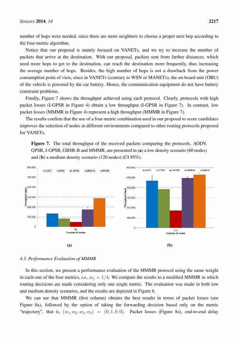
Finally, Figure 7 shows the throughput achieved using each protocol. Clearly, protocols with highpacket losses (I-GPSR in Figure 4) obtain a low throughput (I-GPSR in Figure 7). In contrast, lowpacket losses (MMMR in Figure 4) represent a high throughput (MMMR in Figure 7).

The results confirm that the use of a four-metric combination used in our proposal to score candidatesimproves the selection of nodes in different environments compared to other routing protocols proposedfor VANETs.

Figure 7. The total throughput of the received packets comparing the protocols, AODV,GPSR, I-GPSR, GBSR-B and MMMR, are presented in (a) a low density scenario (60 nodes)and (b) a medium density scenario (120 nodes) (CI 95%).

(a) (b)

4.3. Performance Evaluation of MMMR

In this section, we present a performance evaluation of the MMMR protocol using the same weightin each one of the four metrics, i.e., wj = 1/4. We compare the results to a modified MMMR in whichrouting decisions are made considering only one single metric. The evaluation was made in both lowand medium density scenarios, and the results are depicted in Figure 8.

We can see that MMMR (first column) obtains the best results in terms of packet losses (seeFigure 8a), followed by the option of taking the forwarding decision based only on the metric“trajectory”, that is, (w1, w2, w3, w4) = (0, 1, 0, 0). Packet losses (Figure 8a), end-to-end delay

Sensors 2014, 14 2218

(Figure 8b) and the average number of hops (Figure 8c) are best when the density of the scenario is120 nodes, because the probability of finding a good neighbor is higher than in the case of low densityscenarios (60 nodes). Moreover, in the low density scenario, the probability of using the buffer to storepackets is higher, so that higher delays are obtained. Given that throughput is related to packet losses,we can see that in the medium density scenario, there is a higher throughput (Figure 8d), because lowerlosses were produced (Figure 8a).

Figure 8. The performance of multimetric routing using single metrics in a low (60 nodes)and a medium (120 nodes) density scenario compared to MMMR. The results show: (a) thepercentage of packet losses; (b) the average packet delay; (c) the average number of hops todestination; and (d) the throughput of the received packets (CI 95%).

(a) (b)

(c) (d)

With these results, we can conclude that our proposal based on the use of four metrics to makeforwarding decisions is a good choice to decrease the packet losses in vehicular scenarios and to obtaina low delay in both low and medium density scenarios.

Sensors 2014, 14 2219

Figure 9. The performance of MMMR using four combination of metrics in low (60 nodes)and medium (120 nodes) density scenarios, compared to MMMR using the four metrics.The results show: (a) the percentage of packet losses; (b) the average packet delay; (c) theaverage number of hops to the destination; and (d) the throughput of the received packets(CI 95%).

(a) (b)

(c) (d)

In Figure 9, we present the results of the MMMR protocol compared to another modified versionthat considers only some combinations of metrics. Packet losses are slightly lower in the mediumdensity scenario when forwarding decisions are taken based on the combination of the metric “distance +density”, (w1, w2, w3, w4) = (0.5, 0, 0.5, 0). However, it is not the case in the low density scenario, wherethe best results are obtained with MMMR (w1, w2, w3, w4) = (0.25, 0.25, 0.25, 0.25); see Figure 9a.These results prove that the density of the scenario is a very important parameter in VANETs to obtainthe final score of the candidates to make the forwarding decisions. The behavior of packet delay andthe number of hops in the low density scenario are as expected, i.e., a low number of hops produces ahigh delay, as is the case for the “distance + ABE” combination (w1, w2, w3, w4) = (0.5, 0, 0, 0.5). Thereason is that the use of the buffer, i.e., short paths in low density scenarios, means that packets spent a

Sensors 2014, 14 2220

significant time in the buffer. In the case of the medium density scenario, it shows a quite stable numberof hops and lower delays, because there is a higher number of neighbors, and it was not necessary to usethe local buffer of the nodes often to store packets temporarily until finding a good next forwarder; seeFigure 9a,b.

We can conclude that the metric of the vehicles’ density is decisive in both scenarios, since ithas a high impact on the results. Furthermore, we can notice that it is possible to have goodmetric combinations that improve packet losses and delay, as is the case for “distance + density”(w1, w2, w3, w4) = (0.5, 0, 0.5, 0) in the medium density scenario.

In Tables 5 and 6, we summarize some combination of the weights in the low and medium densityscenarios, respectively. Both tables show the percentage of losses and the average delay obtained witheach combination of weights.

Table 5. A summary of the results of the evaluation of some combination of the weights foreach metric (in a low density scenario). ABE, available bandwidth estimator.

Distance Trajectory Density ABE% Losses

Average Delayw1 w2 w3 w4 [s]

0.25 0.25 0.25 0.25 65.66 1.451 0 0 0 79.17 2.260 1 0 0 70.02 1.560 0 1 0 72.79 1.910 0 0 1 81.14 2.27

0.5 0 0 0.5 83.50 2.880 0.5 0 0.5 71.62 1.54

0.5 0 0.5 0 66.90 1.630 0.5 0.5 0 72.98 2.08

Table 6. A summary of the results of the evaluation of some combination of the weights foreach metric (in a medium density scenario).

Distance Trajectory Density ABE% Losses

Average Delayw1 w2 w3 w4 [s]

0.25 0.25 0.25 0.25 40.58 1.141 0 0 0 44.36 1.220 1 0 0 42.13 1.200 0 1 0 45.47 1.270 0 0 1 53.81 1.40

0.5 0 0 0.5 41.75 1.160 0.5 0 0.5 41.56 1.20

0.5 0 0.5 0 40.29 1.120 0.5 0.5 0 45.75 1.26

Sensors 2014, 14 2221

We can see in Table 5 that the best results, in terms of packet losses and average delay,are obtained with the MMMR combination of weights (w1, w2, w3, w4) = (0.25, 0.25, 0.25, 0.25).In the case of the medium density scenario (see Table 6), the best option is the combination“distance + density” (w1, w2, w3, w4) = (0.5, 0, 0.5, 0). The second best option is our proposal(w1, w2, w3, w4) = (0.25, 0.25, 0.25, 0.25), which, differently from the “distance + density” option,includes a bandwidth guarantee by using the ABE algorithm.

The possible drawback of MMMR is the simple way of assigning weights to each metric,i.e., equitably.

5. Conclusions and Future Work

In this paper, we presented a new routing protocol for VANETs that includes four metrics (distance,trajectory, density and ABE) to make hop-by-hop forwarding decisions. Furthermore, the proposal isbuilding-aware, avoiding those nodes in transmission range, but behind a building. This feature protectspackets from being thrown out. Besides, a local buffer is used to temporarily store those packets whenthe routing protocol fails in finding a proper next forwarding node. We analyzed several metrics anddeveloped an algorithm that includes four of them. The algorithm computes a global score value used toselect the best next forwarding node among all the neighbors in transmission range.

Firstly, we evaluated our proposal compared to other routing proposals present in the literature intwo scenarios (a low and a medium density scenario). In terms of packets losses and throughput,MMMR improves all the protocols evaluated, due to the new way of selecting the next forwarding node.Compared to other existing routing protocols, we concluded that MMMR has a better performance inboth scenarios, low and medium density.

Secondly, we presented a performance evaluation, taking into account the forwarding decision basedon each single metric compared to MMMR. The results show that MMMR, which makes the nextforwarding decision using the equitable combination of the four metrics, is better than making theforwarding decision based only on one of the four metrics independently.

Finally, we evaluated some combinations of the four metrics to analyze the behavior depending onthe scenario. In this evaluation, we noticed that in the case of the 60 node scenario, the best results wereobtained with MMMR. In terms of packet losses, MMMR was followed by the combination of weightsdistance+density, while, in terms of average delay, by the combination of weightsABE+trajectory.This makes sense, since in scenarios with a low density of vehicles, it is better to select nodes that aremoving towards the destination. In the case of the 120 node scenario, the best results are obtained by thedistance+ density combination, followed in second place by MMMR.

As future work, we plan to analyze other methods to obtain a global metric value. Furthermore, thecomputation of the weights of the metrics will be improved in a future work using machine learningtechniques [25] to auto-configure the weights, varying throughout time, making the algorithm adaptableto the changing network conditions that are inherent in VANETs. Finally, we also will explore theavailable power level of each node as a metric to mark nodes as reliable next forwarding nodes.

Sensors 2014, 14 2222

Acknowledgments

This work was partly supported by the Spanish Government through the projects CONSEQUENCE(TEC 2010-20572-C02-02) and TAMESIS (TEC2011-22746). Carolina Tripp and Ahmad Mezherare the recipient of an FI-AGAUR grant of the “Comissionat per a Universitats i Recerca del DIUE”from the Government of Catalonia and the Social European Budget. Carolina also receives a grantfrom the Autonomous University of Sinaloa (Mexico). Luis Urquiza is the recipient of a grantfrom Secretaria Nacional de Educacion Superior, Ciencia y Tecnologıa SENESCYT and the EscuelaPolitecnica Nacional (Ecuador). David Rebollo-Monedero is the recipient of a Juan de la Ciervapostdoctoral fellowship, JCI-2009-05259, from the Spanish Ministry of Science and Innovation.

Author Contributions

Carolina Tripp-Barba developed the analysis of the proposal, conducted simulations, carried outthe analysis of results and took care of most of the writing. Luis Urquiza-Aguiar made most ofthe changes in the code, helped in the analysis of the simulation results and wrote several sections.Monica Aguilar Igartua guided the entire process as well as the analysis of the proposal, made correctionsof the manuscript and wrote some sections. David Rebollo-Monedero contributed to the mathematicalconception and formalization of the metrics. Luis J. de la Cruz Llopis, Ahmad Mohamad Mezher andJose Alfonso Aguilar-Calderon made a general review of the mathematical proposal, assisted with thereview of the simulation results and made corrections throughout the manuscript. All authors participatedin the discussion to develop the proposal and contributed to the analysis of the simulation results, in orderto provide a more comprehensible final version.

Conflicts of Interest

The authors declare no conflict of interest.

References

1. Olariu, S.; Weigle, M. Vehicular Networks: From Theory to Practice; Chapman & Hall/CRCComputer and Information Science Series; Taylor & Francis: Boca Raton, FL, USA, 2009.

2. Hartenstein, H.; Laberteaux, K. VANET Vehicular Applications and Inter-NetworkingTechnologies; Intelligent Transport Systems; Wiley: Chichester, UK, 2009.

3. Papadimitratos, P.; de la Fortelle, A.; Evenssen, K.; Brignolo, R.; Cosenza, S. Vehicularcommunication systems: Enabling technologies, applications, and future outlook on intelligenttransportation. IEEE Commun. Mag. 2009, 47, 84–95.

4. Viriyasitavat, W.; Tonguz, O. Priority Management of Emergency Vehicles at IntersectionsUsing Self-Organized Traffic Control. In Proceedings of the 76th IEEE Vehicular TechnologyConference, Quebec, QC, Canada, 3–6 September 2012; pp. 1–4.

5. Lee, K.; Lee, U.; Gerla, M. Survey of Routing Protocols in Vehicular Ad Hoc Networks. InAdvances in Vehicular Ad-Hoc Networks: Development and Challenges; IGI Global: Hershey, PA,USA , 2009; pp. 149–170.

Sensors 2014, 14 2223

6. Karp, B.; Kung, H.T. GPSR: Greedy Perimeter Stateless Routing for Wireless Networks. InProceedings of the 6th International Conference on Mobile Computing and Networking, Boston,MA, USA, 6–11 August 2006; pp. 243–254.

7. Menouar, H.; Lenardi, M.; Filali, F. Movement Prediction-Based Routing (MOPR) Conceptfor Position-Based Routing in Vehicular Networks. In Proceedings of the 66th IEEE VehicularTechnology Conference, Baltimore, MD, USA, 30 September–3 October 2007; pp. 2101–2105.

8. Granelli, F.; Boato, G.; Kliazovich, D.; Vernazza, G. Enhanced GPSR routing in multi-hopvehicular communications through movement awarness. IEEE Commun. Lett. 2007, 11, 781–783.

9. Naumov, V.; Bauman, R.; Gross, T. An Evaluation of Inter-Vehicle Ad Hoc Networks Based onRealistic Vehicular Traces. In Proceedings of the 7th ACM International Symposium on MobileAd Hoc Networking and Computing, Florence, Italy, 22–25 May 2006; pp. 108–119.

10. Ohta, Y.; Ohta, T.; Kohno, E.; Kakuda, Y. A Store-Carry-Forward-Based Data Transfer SchemeUsing Positions and Moving Direction of Vehicles for Vanets. In Proceedings of the 10thInternational Symposium on Autonomous Decentralized Systems, Tokyo, Japan, 23–27 March2011; pp. 131–138.

11. Xiao, D.; Peng, L.; Asogwa, C.O.; Huang, L. An improved GPSR routing protocol. Int. J. Adv.Comput. Technol. 2011, 3, 132–139.

12. Li, G.; Wang, Y. Routing in vehicular ad hoc networks: A survey. IEEE Veh. Technol. Mag. 2007,2, 12–22.

13. Sarr, C.; Chaudet, C.; Chelius, G.; Guerin-Lassous, I. Bandwidth estimation for IEEE 802.11-basedad hoc networks. IEEE Trans. Mob. Comput. 2008, 7, 1228–1241.

14. Tripp Barba, C.; Mezher, A.M.; Guerin-Lassous, I.; Sarr, C.; Aguilar Igartua, M. AvailableBandwidth-Aware Routing in Urban Vehicular Ad-hoc Networks. In Proceedings of the 76thIEEE Vehicular Technology Conference, Quebec, QC, Canada, 3–6 September 2012; pp. 1–6.

15. Tripp-Barba, C.; Urquiza Aguiar, L.; Aguilar Igartua, M.; Mezher, A.M.; Zaldıvar, A.;Guerin-Lassous, I. Available Bandwidth Estimation in GPSR for VANETs. In Proceedings ofthe 3rd ACM International Symposium on Design and Analysis of Intelligent Vehicular Networksand Applications, Barcelona, Spain, 3–8 November 2013; pp. 1–8.

16. IEEE. 802.11 Standard: Part 11: Wireless LAN Medium Access Control (MAC) and PhysicalLayer (PHY) Specifications. Available online: http://standards.ieee.org/getieee802/download/(accessed on 9 May 2013)

17. Johnson, R.A.; Wichern, D.W. Applied Multivariate Statistical Analysis, 6th ed.; Prentice-Hall, Inc.:Upper Saddle River, NJ, USA, April 2007; pp. 360–413.

18. IBM SPSS Statistics. Available online: http://www-01.ibm.com/software/analytics/spss/ (accessedon 9 May 2013)

19. Perkins, C.E.; Royer, E.M. Ad-hoc On-Demand Distance Vector Routing. In Proceedings of the2nd IEEE workshop on Mobile Computing Systems and Applications, New Orleans, LA, USA,25–26 February 1999; pp. 90–100.

20. Tripp Barba, C.; Urquiza Aguiar, L.; Aguilar Igartua, M. Design and evaluation of GBSR-B, animprovement of GPSR for VANETs. IEEE Lat. Am. Trans. 2013, 11, 1083–1089.

Sensors 2014, 14 2224

21. Wang, S.Y.; Chou, C.L.; Huang, C.H.; Hwang, C.C.; Yang, Z.M.; Chiou, C.C.; Lin, C.C. Thedesign and implementation of the NCTUns 1.0 network simulator. Comput. Netw. 2003, 42,175–197.

22. Wang, S.Y.; Chou, C.L.; Chiu, Y.H.; Tseng, Y.S.; Hsu, M.S.; Cheng, Y.W.; Liu, W.L.; Ho, T.W.NCTUns 4.0: An Integrated Simulation Platform for Vehicular Traffic, Communication, andNetwork Researches. In Proceedings of the 66th IEEE Vehicular Technology Conference,Baltimore, MD, USA, 30 September–3 October 2007; pp. 2081–2085.

23. Martinez, F.; Cano, J.C.; Calafate, C.; Manzoni, P. CityMob: A Mobility Model Pattern Generatorfor VANETs. In Proceedings of the IEEE International Conference on Communications, Beijing,China, 19–23 May 2008; pp. 370–374.

24. Wang, S.Y.; Chou, C.L. NCTUns 5.0: A Network Simulator for IEEE 802.1p and 1609Wireless Vehicular Network Researches. In Proceedings of the 68th IEEE Vehicular TechnologyConference, Calgary, BC, Canada, 21–24 September 2008; pp. 1–2.

25. Mitchel, T. Machine Learning; McGraw-Hill: New York, NY, USA, 1997; pp. 22–47.

c© 2014 by the authors; licensee MDPI, Basel, Switzerland. This article is an open access articledistributed under the terms and conditions of the Creative Commons Attribution license(http://creativecommons.org/licenses/by/3.0/).