i

ney

September, 2009 October, 2009 December 7, 2009

ii

Acknowledgments EPA authors and contributors: Benjamin DeAngelo, Jason Samenow, Jeremy Martinich, Doug Grano, Dina Kruger, Marcus Sarofim, Lesley Jantarasami, William Perkins, Michael Kolian, Melissa Weitz, Leif Hockstad, William Irving, Lisa Hanle, Darrell Winner, David Chalmers, Brian Cook, Chris Weaver, Susan Julius, Brooke Hemming, Sarah Garman, Rona Birnbaum, Paul Argyropoulos, Al McGartland, Alan Carlin, John Davidson, Tim Benner, Carol Holmes, John Hannon, Jim Ketcham-Colwill, Andy Miller, and Pamela Williams. Federal expert reviewers Virginia Burkett, USGS; Phil DeCola; NASA (on detail to OSTP); William Emanuel, NASA; Anne Grambsch, EPA; Jerry Hatfield, USDA; Anthony Janetos; DOE Pacific Northwest National Laboratory; Linda Joyce, USDA Forest Service; Thomas Karl, NOAA; Michael McGeehin, CDC; Gavin Schmidt, NASA; Susan Solomon, NOAA; and Thomas Wilbanks, DOE Oak Ridge National Laboratory. Other contributors: Eastern Research Group (ERG) assisted with document editing and formatting. Stratus Consulting also assisted with document editing and formatting.

iii

Table of Contents Executive Summary..............................................................................................................ES-1 I. Introduction

1. Introduction and Background ..................................................................................................... 2 a. Scope and Approach of This Document.................................................................................... 2 b. Data and Scientific Findings Considered by EPA..................................................................... 4 c. Roadmap for This Document .................................................................................................... 8

II. Greenhouse Gas Emissions

2. Greenhouse Gas Emissions and Concentrations ...................................................................... 11 a. U.S. and Global Greenhouse Gas and Selected Aerosol Emissions........................................ 11 b. Lifetime of Greenhouse Gases in the Atmosphere.................................................................. 16 c. Historic and Current Global Greenhouse Gas Concentrations ............................................... 17

III. Global and U.S. Observed and Projected Effects From Elevated Greenhouse Gas

Concentrations

3. Direct Effects of Elevated Greenhouse Gas Concentrations.................................................... 21

4. Radiative Forcing and Observed Climate Change ................................................................... 23 a. Radiative Forcing Due to Greenhouse Gases and Other Factors ............................................ 23 b. Global Changes in Temperature.............................................................................................. 26 c. U.S. Changes in Temperature.................................................................................................. 32 d. Global Changes in Precipitation.............................................................................................. 34 e. U.S. Changes in Precipitation.................................................................................................. 35 f. Global Sea Level Rise and Ocean Heat Content ..................................................................... 35 g. U.S. Sea Level Rise................................................................................................................. 37 h. Global Ocean Acidification..................................................................................................... 38 i. Global Changes in Physical and Biological Systems .............................................................. 38 j. U.S. Changes in Physical and Biological Systems.................................................................. 41 k. Global Extreme Events............................................................................................................ 43 l. U.S. Extreme Events ............................................................................................................... 44

5. Attribution of Observed Climate Change to Anthropogenic Greenhouse Gas Emissions at

the Global and Continental Scale ............................................................................................... 47 a. Attribution of Observed Climate Change to Anthropogenic Emissions ................................. 47 b. Attribution of Observed Changes in Physical and Biological Systems................................... 53

6. Projected Future Greenhouse Gas Concentrations and Climate Change .............................. 55

a. Global Emissions Scenarios and Associated Changes in Concentrations and Radiative Forcing .................................................................................................................................... 55

b. Projected Changes in Global Temperature, Precipitation Patterns, Sea Level Rise, and Ocean Acidification............................................................................................................................ 63

c. Projected Changes in U.S. Temperature, Precipitation Patterns, and Sea Level Rise............. 68 d. Cryosphere (Snow and Ice) Projections, Focusing on North America and the United States. 72 e. Extreme Events, Focusing on North America and the United States. ..................................... 73

iv

f. Abrupt Climate Change and High-Impact Events................................................................... 75 g. Effects on/from Stratospheric Ozone ...................................................................................... 78 h. Land Use and Land Cover Change.......................................................................................... 80

IV. U.S. Observed and Projected Human Health and Welfare Effects from Climate Change

7. Human Health .............................................................................................................................. 82 a. Temperature Effects ................................................................................................................ 83 b. Extreme Events........................................................................................................................ 85 c. Climate-Sensitive Diseases ..................................................................................................... 86 d. Aeroallergens........................................................................................................................... 88

8. Air Quality.................................................................................................................................... 89

a. Tropospheric Ozone ................................................................................................................ 89 b. Particulate Matter ................................................................................................................... 93 c. Health Effects Due to CO2-Induced Increases in Tropospheric Ozone and Particulate

Matter… ................................................................................................................................ ..96

9. Food Production and Agriculture .............................................................................................. 97 a. Crop Yields and Productivity .................................................................................................. 98 b. Irrigation Requirements......................................................................................................... 100 c. Climate Variability and Extreme Events ............................................................................... 101 d. Pests and Weeds .................................................................................................................... 101 e. Livestock ............................................................................................................................... 102 f. Freshwater and Marine Fisheries........................................................................................... 103

10. Forestry....................................................................................................................................... 104

a. Forest Productivity ............................................................................................................... 105 b. Wildfire and Drought Risk .................................................................................................... 106 c. Forest Composition ............................................................................................................... 108 d. Insects and Diseases .............................................................................................................. 108

11. Water Resources ........................................................................................................................ 110

a. Water Supply and Snowpack ................................................................................................ 110 b. Water Quality ........................................................................................................................ 113 c. Extreme Events...................................................................................................................... 115 d. Implications for Water Uses.................................................................................................. 116

12. Sea Level Rise and Coastal Areas............................................................................................. 117

a. Vulnerable Areas .................................................................................................................. 117 b. Extreme Events...................................................................................................................... 120

13. Energy, Infrastructure, and Settlements ................................................................................. 122

a. Heating and Cooling Requirements....................................................................................... 122 b. Energy Production................................................................................................................. 123 c. Infrastructure and Settlements............................................................................................... 125

14. Ecosystems and Wildlife............................................................................................................ 131

a. Ecosystems and Species ........................................................................................................ 131 b. Ecosystem Services ............................................................................................................... 138 c. Extreme Events...................................................................................................................... 139

v

d. Implications for Tribes .......................................................................................................... 139 e. Implications for Tourism....................................................................................................... 140

15. U.S. Regional Climate Change Impacts ................................................................................... 141

a. Northeast ............................................................................................................................... 142 b. Southeast ............................................................................................................................... 143 c. Midwest ................................................................................................................................. 144 d. Great Plains ........................................................................................................................... 146 e. Southwest .............................................................................................................................. 148 f. Northwest .............................................................................................................................. 150 g. Alaska.................................................................................................................................... 152 h. Islands.................................................................................................................................... 153

V. Observed and Projected Human Health and Welfare Effects From Climate Change in

Other World Regions

16. Impacts in Other World Regions .............................................................................................. 157 a. National Security Concerns................................................................................................... 157 b. Overview of International Impacts ........................................................................................ 159

References............................................................................................................................... 164 Appendix A: Brief Overview of Adaptation .......................................................................... 176 Appendix B: Greenhouse Gas Emissions From Section 202(a) Source Categories ........ 180 Appendix C: Direct Effects of GHGs on Human Health....................................................... 195

ES-1

Executive Summary This document provides technical support for the endangerment and cause or contribute analyses concerning greenhouse gas (GHG) emissions under section 202(a) of the Clean Air Act. This document itself does not convey any judgment or conclusion regarding the question of whether GHGs may be reasonably anticipated to endanger public health or welfare, as this decision is ultimately left to the judgment of the Administrator. The conclusions here and the information throughout this document are primarily drawn from the assessment reports of the Intergovernmental Panel on Climate Change (IPCC), the U.S. Climate Change Science Program (CCSP), the U.S. Global Change Research Program (USGCRP), and the National Research Council (NRC). Observed Trends in Greenhouse Gas Emissions and Concentrations Greenhouse gases, once emitted, can remain in the atmosphere for decades to centuries, meaning that 1) their concentrations become well-mixed throughout the global atmosphere regardless of emission origin, and 2) their effects on climate are long lasting. The primary long-lived GHGs directly emitted by human activities include carbon dioxide (CO2), methane (CH4), nitrous oxide (N2O), hydrofluorocarbons (HFCs), perfluorocarbons (PFCs), and sulfur hexafluoride (SF6). Greenhouse gases have a warming effect by trapping heat in the atmosphere that would otherwise escape to space. In 2007, U.S. GHG emissions were 7,150 teragrams1 of CO2 equivalent2 (TgCO2eq). The dominant gas emitted is CO2, mostly from fossil fuel combustion. Methane is the second largest component of U.S. emissions, followed by N2O and the fluorinated gases (HFCs, PFCs, and SF6). Electricity generation is the largest emitting sector (34% of total U.S. GHG emissions), followed by transportation (28%) and industry (19%). Transportation sources under Section 202 of the Clean Air Act (passenger cars, light duty trucks, other trucks and buses, motorcycles, and cooling) emitted 1,649 TgCO2eq in 2007, representing 23% of total U.S. GHG emissions. U.S. transportation sources under Section 202 made up 4.3% of total global GHG emissions in 2005, which, in addition to the United States as a whole, ranked only behind total GHG emissions from China, Russia, and India but ahead of Japan, Brazil, Germany, and the rest of the world’s countries. In 2005, total U.S. GHG emissions were responsible for 18% of global emissions, ranking only behind China, which was responsible for 19% of global GHG emissions. U.S. emissions of sulfur oxides (SOx), nitrogen oxides (NOx), direct particulates, and ozone precursors have decreased in recent decades, due to regulatory actions and improvements in technology. Sulfur dioxide (SO2) emissions in 2007 were 5.9 Tg of sulfur, primary fine particulate matter (PM2.5) emissions in 2005 were 5.0 Tg, NOx emissions in 2005 were 18.5 Tg, volatile organic compound (VOC) emissions in 2005 were 16.8 Tg, and ammonia emissions in 2005 were 3.7 Tg. The global atmospheric CO2 concentration has increased about 38% from pre-industrial levels to 2009, and almost all of the increase is due to anthropogenic emissions. The global atmospheric

1 One teragram (Tg) = 1 million metric tons. 1 metric ton = 1,000 kilograms = 1.102 short tons = 2,205 pounds. 2 Long-lived GHGs are compared and summed together on a CO2-equivalent basis by multiplying each gas by its global warming potential (GWP), as estimated by IPCC. In accordance with United Nations Framework Convention on Climate Change (UNFCCC) reporting procedures, the U.S. quantifies GHG emissions using the 100-year timeframe values for GWPs established in the IPCC Second Assessment Report.

ES-2

concentration of CH4 has increased by 149% since pre-industrial levels (through 2007); and the N2O concentration has increased by 23% (through 2007). The observed concentration increase in these gases can also be attributed primarily to anthropogenic emissions. The industrial fluorinated gases, HFCs, PFCs, and SF6, have relatively low atmospheric concentrations but the total radiative forcing due to these gases is increasing rapidly; these gases are almost entirely anthropogenic in origin. Historic data show that current atmospheric concentrations of the two most important directly emitted, long-lived GHGs (CO2 and CH4) are well above the natural range of atmospheric concentrations compared to at least the last 650,000 years. Atmospheric GHG concentrations have been increasing because anthropogenic emissions have been outpacing the rate at which GHGs are removed from the atmosphere by natural processes over timescales of decades to centuries. Observed Effects Associated With Global Elevated Concentrations of GHGs Current ambient air concentrations of CO2 and other GHGs remain well below published exposure thresholds for any direct adverse health effects, such as respiratory or toxic effects. The global average net effect of the increase in atmospheric GHG concentrations, plus other human activities (e.g., land-use change and aerosol emissions), on the global energy balance since 1750 has been one of warming. This total net heating effect, referred to as forcing, is estimated to be +1.6 (+0.6 to +2.4) watts per square meter (W/m2), with much of the range surrounding this estimate due to uncertainties about the cooling and warming effects of aerosols. However, as aerosol forcing has more regional variability than the well-mixed, long-lived GHGs, the global average might not capture some regional effects. The combined radiative forcing due to the cumulative (i.e., 1750 to 2005) increase in atmospheric concentrations of CO2, CH4, and N2O is estimated to be +2.30 (+2.07 to +2.53) W/m2. The rate of increase in positive radiative forcing due to these three GHGs during the industrial era is very likely to have been unprecedented in more than 10,000 years. Warming of the climate system is unequivocal, as is now evident from observations of increases in global average air and ocean temperatures, widespread melting of snow and ice, and rising global average sea level. Global mean surface temperatures have risen by 1.3 ± 0.32F (0.74°C ± 0.18C) over the last 100 years. Eight of the 10 warmest years on record have occurred since 2001. Global mean surface temperature was higher during the last few decades of the 20th century than during any comparable period during the preceding four centuries. Most of the observed increase in global average temperatures since the mid-20th century is very likely due to the observed increase in anthropogenic GHG concentrations. Climate model simulations suggest natural forcing alone (i.e., changes in solar irradiance) cannot explain the observed warming. U.S. temperatures also warmed during the 20th and into the 21st century; temperatures are now approximately 1.3°F (0.7°C) warmer than at the start of the 20th century, with an increased rate of warming over the past 30 years. Both the IPCC and the CCSP reports attributed recent North American warming to elevated GHG concentrations. In the CCSP (2008g) report, the authors find that for North America, “more than half of this warming [for the period 1951-2006] is likely the result of human-caused greenhouse gas forcing of climate change.” Observations show that changes are occurring in the amount, intensity, frequency and type of precipitation. Over the contiguous United States, total annual precipitation increased by 6.1% from 1901 to 2008. It is likely that there have been increases in the number of heavy precipitation events within

ES-3

many land regions, even in those where there has been a reduction in total precipitation amount, consistent with a warming climate. There is strong evidence that global sea level gradually rose in the 20th century and is currently rising at an increased rate. It is not clear whether the increasing rate of sea level rise is a reflection of short-term variability or an increase in the longer-term trend. Nearly all of the Atlantic Ocean shows sea level rise during the last 50 years with the rate of rise reaching a maximum (over 2 millimeters [mm] per year) in a band along the U.S. east coast running east-northeast. Satellite data since 1979 show that annual average Arctic sea ice extent has shrunk by 4.1% per decade. The size and speed of recent Arctic summer sea ice loss is highly anomalous relative to the previous few thousands of years. Widespread changes in extreme temperatures have been observed in the last 50 years across all world regions, including the United States. Cold days, cold nights, and frost have become less frequent, while hot days, hot nights, and heat waves have become more frequent. Observational evidence from all continents and most oceans shows that many natural systems are being affected by regional climate changes, particularly temperature increases. However, directly attributing specific regional changes in climate to emissions of GHGs from human activities is difficult, especially for precipitation. Ocean CO2 uptake has lowered the average ocean pH (increased acidity) level by approximately 0.1 since 1750. Consequences for marine ecosystems can include reduced calcification by shell-forming organisms, and in the longer term, the dissolution of carbonate sediments. Observations show that climate change is currently affecting U.S. physical and biological systems in significant ways. The consistency of these observed changes in physical and biological systems and the observed significant warming likely cannot be explained entirely due to natural variability or other confounding non-climate factors. Projections of Future Climate Change With Continued Increases in Elevated GHG Concentrations Most future scenarios that assume no explicit GHG mitigation actions (beyond those already enacted) project increasing global GHG emissions over the century, with climbing GHG concentrations. Carbon dioxide is expected to remain the dominant anthropogenic GHG over the course of the 21st century. The radiative forcing associated with the non-CO2 GHGs is still significant and increasing over time. Future warming over the course of the 21st century, even under scenarios of low-emission growth, is very likely to be greater than observed warming over the past century. According to climate model simulations summarized by the IPCC, through about 2030, the global warming rate is affected little by the choice of different future emissions scenarios. By the end of the 21st century, projected average global warming (compared to average temperature around 1990) varies significantly depending on the emission scenario and climate sensitivity assumptions, ranging from 3.2 to 7.2F (1.8 to 4.0C), with an uncertainty range of 2.0 to 11.5F (1.1 to 6.4C). All of the United States is very likely to warm during this century, and most areas of the United States are expected to warm by more than the global average. The largest warming is projected to occur in winter over northern parts of Alaska. In western, central and eastern regions of North America,

ES-4

the projected warming has less seasonal variation and is not as large, especially near the coast, consistent with less warming over the oceans. It is very likely that heat waves will become more intense, more frequent, and longer lasting in a future warm climate, whereas cold episodes are projected to decrease significantly. Increases in the amount of precipitation are very likely in higher latitudes, while decreases are likely in most subtropical latitudes and the southwestern United States, continuing observed patterns. The mid-continental area is expected to experience drying during summer, indicating a greater risk of drought. Intensity of precipitation events is projected to increase in the United States and other regions of the world. More intense precipitation is expected to increase the risk of flooding and result in greater runoff and erosion that has the potential for adverse water quality effects. It is likely that hurricanes will become more intense, with stronger peak winds and more heavy precipitation associated with ongoing increases of tropical sea surface temperatures. Frequency changes in hurricanes are currently too uncertain for confident projections. By the end of the century, global average sea level is projected by IPCC to rise between 7.1 and 23 inches (18 and 59 centimeter [cm]), relative to around 1990, in the absence of increased dynamic ice sheet loss. Recent rapid changes at the edges of the Greenland and West Antarctic ice sheets show acceleration of flow and thinning. While an understanding of these ice sheet processes is incomplete, their inclusion in models would likely lead to increased sea level projections for the end of the 21st century. Sea ice extent is projected to shrink in the Arctic under all IPCC emissions scenarios. Projected Risks and Impacts Associated With Future Climate Change Risk to society, ecosystems, and many natural Earth processes increase with increases in both the rate and magnitude of climate change. Climate warming may increase the possibility of large, abrupt regional or global climatic events (e.g., disintegration of the Greenland Ice Sheet or collapse of the West Antarctic Ice Sheet). The partial deglaciation of Greenland (and possibly West Antarctica) could be triggered by a sustained temperature increase of 2 to 7F (1 to 4ºC) above 1990 levels. Such warming would cause a 13 to 20 feet (4 to 6 meter) rise in sea level, which would occur over a time period of centuries to millennia. CCSP reports that climate change has the potential to accentuate the disparities already evident in the American health care system, as many of the expected health effects are likely to fall disproportionately on the poor, the elderly, the disabled, and the uninsured. IPCC states with very high confidence that climate change impacts on human health in U.S. cities will be compounded by population growth and an aging population. Severe heat waves are projected to intensify in magnitude and duration over the portions of the United States where these events already occur, with potential increases in mortality and morbidity, especially among the elderly, young, and frail. Some reduction in the risk of death related to extreme cold is expected. It is not clear whether reduced mortality from cold will be greater or less than increased heat-related mortality in the United States due to climate change.

ES-5

Increases in regional ozone pollution relative to ozone levels without climate change are expected due to higher temperatures and weaker circulation in the United States and other world cities relative to air quality levels without climate change. Climate change is expected to increase regional ozone pollution, with associated risks in respiratory illnesses and premature death. In addition to human health effects, tropospheric ozone has significant adverse effects on crop yields, pasture and forest growth, and species composition. The directional effect of climate change on ambient particulate matter levels remains uncertain. Within settlements experiencing climate change, certain parts of the population may be especially vulnerable; these include the poor, the elderly, those already in poor health, the disabled, those living alone, and/or indigenous populations dependent on one or a few resources. Thus, the potential impacts of climate change raise environmental justice issues. CCSP concludes that, with increased CO2 and temperature, the life cycle of grain and oilseed crops will likely progress more rapidly. But, as temperature rises, these crops will increasingly begin to experience failure, especially if climate variability increases and precipitation lessens or becomes more variable. Furthermore, the marketable yield of many horticultural crops (e.g., tomatoes, onions, fruits) is very likely to be more sensitive to climate change than grain and oilseed crops. Higher temperatures will very likely reduce livestock production during the summer season in some areas, but these losses will very likely be partially offset by warmer temperatures during the winter season. Cold-water fisheries will likely be negatively affected; warm-water fisheries will generally benefit; and the results for cool-water fisheries will be mixed, with gains in the northern and losses in the southern portions of ranges. Climate change has very likely increased the size and number of forest fires, insect outbreaks, and tree mortality in the interior West, the Southwest, and Alaska, and will continue to do so. Over North America, forest growth and productivity have been observed to increase since the middle of the 20th century, in part due to observed climate change. Rising CO2 will very likely increase photosynthesis for forests, but the increased photosynthesis will likely only increase wood production in young forests on fertile soils. The combined effects of expected increased temperature, CO2, nitrogen deposition, ozone, and forest disturbance on soil processes and soil carbon storage remain unclear. Coastal communities and habitats will be increasingly stressed by climate change impacts interacting with development and pollution. Sea level is rising along much of the U.S. coast, and the rate of change will very likely increase in the future, exacerbating the impacts of progressive inundation, storm-surge flooding, and shoreline erosion. Storm impacts are likely to be more severe, especially along the Gulf and Atlantic coasts. Salt marshes, other coastal habitats, and dependent species are threatened by sea level rise, fixed structures blocking landward migration, and changes in vegetation. Population growth and rising value of infrastructure in coastal areas increases vulnerability to climate variability and future climate change. Climate change will likely further constrain already overallocated water resources in some regions of the United States, increasing competition among agricultural, municipal, industrial, and ecological uses. Although water management practices in the United States are generally advanced, particularly in the West, the reliance on past conditions as the basis for current and future planning may no longer be appropriate, as climate change increasingly creates conditions well outside of historical observations. Rising temperatures will diminish snowpack and increase evaporation, affecting seasonal

ES-6

availability of water. In the Great Lakes and major river systems, lower water levels are likely to exacerbate challenges relating to water quality, navigation, recreation, hydropower generation, water transfers, and binational relationships. Decreased water supply and lower water levels are likely to exacerbate challenges relating to aquatic navigation in the United States. Higher water temperatures, increased precipitation intensity, and longer periods of low flows will exacerbate many forms of water pollution, potentially making attainment of water quality goals more difficult. As waters become warmer, the aquatic life they now support will be replaced by other species better adapted to warmer water. In the long term, warmer water and changing flow may result in deterioration of aquatic ecosystems. Ocean acidification is projected to continue, resulting in the reduced biological production of marine calcifiers, including corals. Climate change is likely to affect U.S. energy use and energy production and physical and institutional infrastructures. It will also likely interact with and possibly exacerbate ongoing environmental change and environmental pressures in settlements, particularly in Alaska where indigenous communities are facing major environmental and cultural impacts. The U.S. energy sector, which relies heavily on water for hydropower and cooling capacity, may be adversely impacted by changes to water supply and quality in reservoirs and other water bodies. Water infrastructure, including drinking water and wastewater treatment plants, and sewer and stormwater management systems, will be at greater risk of flooding, sea level rise and storm surge, low flows, and other factors that could impair performance. Disturbances such as wildfires and insect outbreaks are increasing in the United States and are likely to intensify in a warmer future with warmer winters, drier soils, and longer growing seasons. Although recent climate trends have increased vegetation growth, continuing increases in disturbances are likely to limit carbon storage, facilitate invasive species, and disrupt ecosystem services. Over the 21st century, changes in climate will cause species to shift north and to higher elevations and fundamentally rearrange U.S. ecosystems. Differential capacities for range shifts and constraints from development, habitat fragmentation, invasive species, and broken ecological connections will alter ecosystem structure, function, and services. Climate change impacts will vary in nature and magnitude across different regions of the United States. Sustained high summer temperatures, heat waves, and declining air quality are projected in the

Northeast3, Southeast4, Southwest5, and Midwest6. Projected climate change would continue to cause loss of sea ice, glacier retreat, permafrost thawing, and coastal erosion in Alaska.

Reduced snowpack, earlier spring snowmelt, and increased likelihood of seasonal summer droughts are projected in the Northeast, Northwest7, and Alaska. More severe, sustained droughts and water scarcity are projected in the Southeast, Great Plains8, and Southwest.

3 Northeast includes West Virginia, Maryland, Delaware, Pennsylvania, New Jersey, New York, Connecticut, Rhode Island, Massachusetts, Vermont, New Hampshire, and Maine. 4 Southeast includes Kentucky, Virginia, Arkansas, Tennessee, North Carolina, South Carolina, southeast Texas, Louisiana, Mississippi, Alabama, Georgia, and Florida. 5 Southwest includes California, Nevada, Utah, western Colorado, Arizona, New Mexico (except the extreme eastern section), and southwest Texas. 6 The Midwest includes Minnesota, Wisconsin, Michigan, Iowa, Illinois, Indiana, Ohio, and Missouri. 7 The Northwest includes Washington, Idaho, western Montana, and Oregon.

ES-7

The Southeast, Midwest, and Northwest in particular are expected to be impacted by an increased frequency of heavy downpours and greater flood risk.

Ecosystems of the Southeast, Midwest, Great Plains, Southwest, Northwest, and Alaska are expected to experience altered distribution of native species (including local extinctions), more frequent and intense wildfires, and an increase in insect pest outbreaks and invasive species.

Sea level rise is expected to increase storm surge height and strength, flooding, erosion, and wetland loss along the coasts, particularly in the Northeast, Southeast, and islands.

Warmer water temperatures and ocean acidification are expected to degrade important aquatic resources of islands and coasts such as coral reefs and fisheries.

A longer growing season, low levels of warming, and fertilization effects of carbon dioxide may benefit certain crop species and forests, particularly in the Northeast and Alaska. Projected summer rainfall increases in the Pacific islands may augment limited freshwater supplies. Cold-related mortality is projected to decrease, especially in the Southeast. In the Midwest in particular, heating oil demand and snow-related traffic accidents are expected to decrease.

Climate change impacts in certain regions of the world may exacerbate problems that raise humanitarian, trade, and national security issues for the United States. The IPCC identifies the most vulnerable world regions as the Arctic, because of the effects of high rates of projected warming on natural systems; Africa, especially the sub-Saharan region, because of current low adaptive capacity as well as climate change; small islands, due to high exposure of population and infrastructure to risk of sea level rise and increased storm surge; and Asian mega-deltas, such as the Ganges-Brahmaputra and the Zhujiang, due to large populations and high exposure to sea level rise, storm surge and river flooding. Climate change has been described as a potential threat multiplier with regard to national security issues.

8 The Great Plains includes central and eastern Montana, North Dakota, South Dakota, Wyoming, Nebraska, eastern Colorado, Nebraska, Kansas, extreme eastern New Mexico, central Texas, and Oklahoma

1

Part I

Introduction

2

Section 1 Introduction and Background The purpose of this Technical Support Document (TSD) is to provide scientific and technical information for an endangerment and cause or contribute analysis regarding greenhouse gas (GHG) emissions from new motor vehicles and engines under Section 202(a) of the Clean Air Act. Section 202 (a)(1) of the Clean Air Act states that:

the Administrator shall by regulation prescribe (and from time to time revise)…standards applicable to the emission of any air pollutant from any class or classes of new motor vehicles …, which in his judgment cause, or contribute to, air pollution which may reasonably be anticipated to endanger public health or welfare.

Thus before EPA may issue standards addressing emissions of an air pollutant from new motor vehicles or new motor vehicle engines under Section 202(a), the Administrator must make a so-called “endangerment finding.” That finding is a two-step test. First, the Administrator must decide if, in her judgment, air pollution may reasonably be anticipated to endanger public health or welfare. Second, the Administrator must decide whether, in her judgment, emissions of any air pollutant from new motor vehicles or engines cause or contribute to this air pollution. If the Administrator answers both questions in the affirmative, EPA shall issue standards under Section 202(a). This document itself does not convey any judgment or conclusion regarding the two steps of the endangerment finding, as these decisions are ultimately left to the judgment of the Administrator. Readers should refer to the Final Endangerment and Cause or Contribute Findings for Greenhouse Gases (signed December 7, 2009) for a discussion of how the Administrator considered the information contained in this TSD in her determinations regarding the endangerment and cause or contribute findings. This TSD has been revised and updated since the version of this document released April 17, 2009, to accompany the Administrator’s proposed endangerment and cause or contribute findings (74 FR 18886, EPA-HQ-OAR-2009-0171). The proposed findings and TSD were subject to a 60-day public comment period as well as two public hearings. An earlier version of the TSD was released July 11, 2008, to accompany the Advance Notice of Proposed Rulemaking on the Regulation of Greenhouse Gases under the Clean Air Act (73 FR 44353, EPA-HQ-OAR-2008-0318), which was subject to a 120-day public comment period. The draft released in April 2009 has been revised to reflect the most up-to-date GHG emissions and climate data, a new major scientific assessment by the U.S. Global Change Research Program (USGCRP), and EPA’s responses to significant public comments pertaining to the draft TSD.9 The remainder of this introductory chapter explains the scope and approach of this document and the underlying references and data sources on which it relies. 1(a) Scope and Approach of This Document The primary GHGs that are directly emitted by human activities in general are those reported in EPA’s annual Inventory of U.S. Greenhouse Gas Emissions and Sinks and include carbon dioxide (CO2), methane (CH4), nitrous oxide (N2O), hydrofluorocarbons (HFCs), perfluorocarbons (PFCs) and sulfur hexafluoride (SF6). The primary effect of these gases is their influence on the climate system by trapping

9 Detailed responses to all significant public comments received on the Administrator’s Proposed Endangerment and Cause or Contribute Findings released on April 17, 2009, can be found in the separate Response to Comments document.

3

heat in the atmosphere that would otherwise escape to space. This heating effect (referred to as radiative forcing) is very likely to be the cause of most of the observed global warming over the last 50 years. Global warming and climate change can, in turn, affect health, society, and the environment. There also are some cases where these gases have other non-climate effects. For example, elevated concentrations of CO2 can lead to ocean acidification and stimulate terrestrial plant growth, and CH4 emissions can contribute to background levels of tropospheric ozone, a criteria pollutant. These effects can in turn be influenced by climate change in certain cases. Carbon dioxide and other GHGs can also have direct health effects but at concentrations far in excess of current or projected future ambient concentrations. There are other known anthropogenic forcing agents that influence climate, such as changes in land use, which can in turn change surface reflectivity, as well as emissions of aerosols, which can have both heating and cooling influences on the climate. These other forcing agents are discussed as well to place the anthropogenic GHG influence in context. This document reviews a wide range of observed and projected vulnerabilities, risks, and impacts due to the elevated levels of GHGs in the atmosphere and associated climate change. Any known or expected benefits of elevated atmospheric concentrations of GHGs or of climate change are documented as well (recognizing that climate impacts can have both positive and negative consequences). The extent to which observed climate change can be attributed to anthropogenic GHG emissions is assessed. The term “climate change” in this document generally refers to climate change induced by human activities, including activities that emit GHGs. Future projections of climate change, based primarily on future scenarios of anthropogenic GHG emissions, are shown for the global and national scale. The vulnerability, risk, and impact assessment in this document primarily focuses on the United States. However, given the global nature of climate change, there is a brief review of potential impacts in other regions of the world. Greenhouse gases, once emitted, become well mixed in the atmosphere, meaning U.S. emissions can affect not only the U.S. population and environment but other regions of the world as well; likewise, emissions in other countries can affect the United States. Furthermore, impacts in other regions of the world may have consequences that in turn raise humanitarian, trade, and national security concerns for the United States. The timeframe over which vulnerabilities, risks, and impacts are considered is consistent with the timeframe over which GHGs, once emitted, have an effect on climate, which is decades to centuries for the primary GHGs of concern. Therefore, in addition to reviewing recent observations, this document generally considers the next several decades, until approximately 2100, and for certain impacts, beyond 2100. Adaptation to climate change is a key focus area of the climate change research community. This document, however, does not assess the climate change impacts in light of potential adaptation measures. This is because adaptation is essentially a response to any known and/or perceived risks due to climate change. Likewise, mitigation measures to reduce GHGs, which could also reduce long-term risks, are not explicitly addressed. The purpose of this document is to review the effects of climate change and not to assess any potential policy or societal response to climate change. There are cases in this document, however, where some degree of adaptation is accounted for; these cases occur where the literature on which this document relies already incorporates information about adaptation that has already occurred or uses assumptions about adaptation when projecting the future effects of climate change. Such cases are noted in the document.10

10 A brief overview of adaptation is provided in Appendix A.

4

1(b) Data and Scientific Findings Considered by EPA This document relies most heavily on existing, and in most cases very recent, synthesis reports of climate change science and potential impacts, which have undergone their own peer-review processes, including review by the U.S. government. Box 1.1 describes this process11. The information in this document has been developed and prepared in a manner that is consistent with EPA's Guidelines for Ensuring and Maximizing the Quality, Objectivity, Utility and Integrity of Information Disseminated by the Environmental Protection Agency (U.S. EPA 2002). In addition to its reliance on existing and recent synthesis reports, which have each gone through extensive peer-review procedures, this document also underwent a technical review by 12 federal climate change experts, internal EPA review, interagency review, and a public comment period. Box 1.1: Peer Review, Publication, and Approval Processes for IPCC, CCSP/USGCRP, and NRC Reports Intergovernmental Panel on Climate Change The World Meteorological Organization (WMO) and the United Nations Environment Programme (UNEP) established the Intergovernmental Panel on Climate Change (IPCC) in 1988. It bases its assessment mainly on peer reviewed and published scientific/technical literature. IPCC has established rules and procedures for producing its assessment reports. Report outlines are agreed to by government representatives in consultation with the IPCC bureau. Lead authors are nominated by governments and are selected by the respective IPCC Working Groups on the basis of their scientific credentials and with due consideration for broad geographic representation. For Working Group I (The Physical Science Basis) there were 152 coordinating lead authors, and for Working Group II (Impacts, Adaptation and Vulnerability) there were 48 coordinating lead authors. Drafts prepared by the authors are subject to two rounds of review; the first round is technical (or “expert” in the IPCC lexicon), and the second round includes government review. For the IPCC Working Group I report, more than 30,000 written comments were submitted by over 650 individual experts, governments, and international organizations. For Working Group II there were 910 expert reviewers. Under the IPCC procedures, review editors for each chapter are responsible for ensuring that all substantive government and expert review comments receive appropriate consideration. For transparency, IPCC documents how every comment is addressed. Each Summary for Policymakers is approved line-by-line, and the underlying chapters then accepted, by government delegations in formal plenary sessions. Further information about IPCC’s (2009) principles and procedures can be found at: http://www.ipcc.ch/organization/organization_procedures.htm. U.S. Climate Change Science Program and U.S. Global Change Research Program Under the Bush Administration, the U.S. Climate Change Science Program (CCSP) integrated federal research on climate and global change, as sponsored by thirteen federal agencies and overseen by the Office of Science and Technology Policy, the Council on Environmental Quality, the National Economic Council and the Office of Management and Budget. As of January 16, 2009, the CCSP had completed 21 synthesis and assessment products (SAPs) that address the highest priorities for U.S. climate change research, observation, and decision support needs. Different agencies were designated the lead for different SAPs; EPA was the designated lead for three of the six SAPs addressing impacts and adaptation. For each SAP, there was first a prospectus that provided an outline, the proposed authors, and the process for completing the SAP; this went through two stages of expert, interagency, and public review. Authors produced a first draft that went through expert review; a second draft was posted for public review. The designated lead agency ensured that the third draft complied with the Information Quality Act. Finally, each SAP was submitted for approval by the National Science and Technology Council (NSTC), a cabinet-level council that coordinates science and technology research across the federal government. Further information about the clearance and review procedures for the CCSP SAPs can be found at: http://www.climatescience.gov/Library/sap/sap-guidelines-clarification-aug2007.htm. In June 2009, the U.S. Global Change Research Program (which had been incorporated under the CCSP during the

11 Volume 1 of EPA’s Response to Comments document on the on the Administrator’s Endangerment and Cause or Contribute Findings, provides more detailed information on these review processes.

5

Bush Administration, but, as of January 2009, was re-established as the comprehensive and integrating body for global change research, subsuming CCSP and its products) completed an assessment, Global Climate Change Impacts in the United States that incorporated all 21 SAPs from the CCSP, as well as the IPCC Fourth Assessment Report. As stated in that report, “This report meets all Federal requirements associated with the Information Quality Act, including those pertaining to public comment and transparency.” National Research Council of the U.S. National Academy of Sciences The National Research Council (NRC) is part of the National Academies, which also comprise the National Academy of Sciences, National Academy of Engineering and Institute of Medicine. They are private, nonprofit institutions that provide science, technology, and health policy advice under a congressional charter. The NRC has become the principal operating agency of both the National Academy of Sciences and the National Academy of Engineering in providing services to the government, the public, and the scientific and engineering communities. Federal agencies are the primary financial sponsors of the Academies’ work. The Academies provide independent advice; the external sponsors have no control over the conduct of a study once the statement of task and budget are finalized. The NRC (2001a) study, Climate Change Science: An Analysis of Some Key Questions, originated from a White House request. The NRC (2001b) study, Global Air Quality: An Imperative for Long-Term Observational Strategies, was supported by EPA and NASA. The NRC 2004 study, Air Quality Management in the United States, was supported by EPA. The NRC 2005 study, Radiative Forcing of Climate Change: Expanding the Concept and Addressing Uncertainties, was in response to a CCSP request and was supported by NOAA. The NRC (2006b) study, Surface Temperature Reconstructions for the Last 2,000 Years, was requested by the Science Committee of the U.S. House of Representatives. Each NRC report is authored by its own committee of experts, reviewed by outside experts, and approved by the Governing Board of the NRC. Table 1.1 lists the core reference documents for this TSD. These include the 2007 Fourth Assessment Report of the Intergovernmental Panel on Climate Change (IPCC), the Synthesis and Assessment Products of the U.S. Climate Change Science Program (CCSP) published between 2006 and 2009, the 2009 USGCRP scientific assessment, National Research Council (NRC) reports under the U.S. National Academy of Sciences (NAS), the National Oceanic and Atmospheric Administration’s (NOAA’s) 2009 State of the Climate in 2008 report, the 2009 EPA annual U.S. Inventory of Greenhouse Gas Emissions and Sinks, and the 2009 EPA assessment of the impacts of global change on regional U.S. air quality. This version of the TSD, as well as previous versions of the TSD dating back to 2007, have taken the approach of relying primarily on these assessment reports because they 1) are very recent and represent the current state of knowledge on GHG emissions, climate change science, vulnerabilities, and potential impacts; 2) have assessed numerous individual, peer-reviewed studies in order to draw general conclusions about the state of science; 3) have been reviewed and formally accepted, commissioned, or in some cases authored by U.S. government agencies and individual government scientists; and 4) they reflect and convey the consensus conclusions of expert authors. Box 1.1 describes the peer review and publication approval processes of IPCC, CCSP/USGCRP and NRC reports. Peer review and transparency are central to each of these research organizations’ report development process. Given the comprehensiveness of these assessments and their review processes, these assessment reports provide EPA with assurances that this material has been well vetted by both the climate change research community and by the U.S. government. Furthermore, use of these assessments complies with EPA’s information quality guidelines, as this document relies on information that is objective, technically sound and vetted, and of high integrity.12

12 The Response to Comments document, which also accompanies the Administrator’s final Endangerment and Cause or Contribute Findings, contains additional information about EPA’s responses to comments received about EPA’s use of assessment reports such as those from IPCC and USGCRP, as well as issues concerning the Data Quality Act.

6

Uncertainties and confidence levels associated with the scientific conclusions and findings in this document are reported, to the extent that such information was provided in the original scientific reports upon which this document is based. Box 1.2 describes the lexicon used by IPCC to communicate uncertainty and confidence levels associated with the most important IPCC findings. The CCSP and USGCRP generally adopted the same lexicon with their respective definitions. Therefore, this document employs the same lexicon when referencing IPCC, CCSP and USGCRP statements.

Table 1.1 Core references relied upon most heavily in this document.

Science Body/Author Short Title and Year of Publication

NOAA State of the Climate in 2008 (2009)

USGCRP Global Climate Change Impacts in the United States (2009)

IPCC Working Group I: The Physical Science Basis (2007)

IPCC Working Group II: Impacts, Adaptation and Vulnerability (2007)

IPCC Working Group III: Mitigation of Climate Change (2007)

CCSP SAP 1.1: Temperature Trends in the Lower Atmosphere (2006)

CCSP SAP 1.2: Past Climate Variability and Change in the Arctic and at High Latitudes (2009)

CCSP SAP 1.3: Re-analyses of Historical Climate Data (2008)

CCSP SAP 2.1: Scenarios of GHG Emissions and Atmospheric Concentrations (2007)

CCSP SAP 2.3: Aerosol Properties and their Impacts on Climate

CCSP SAP 2.4: Trends in Ozone-Depleting Substances (2008)

CCSP SAP 3.1: Climate Change Models (2008)

CCSP SAP 3.2: Climate Projections (2008)

CCSP SAP 3.3: Weather and Climate Extremes in a Changing Climate (2008)

CCSP SAP 3.4: Abrupt Climate Change (2008)

CCSP SAP 4.1: Coastal Sensitivity to Sea Level Rise (2009)

CCSP SAP 4.2: Thresholds of Change in Ecosystems (2009)

CCSP SAP 4.3: Agriculture, Land Resources, Water Resources, and Biodiversity (2008)

CCSP SAP 4.5: Effects on Energy Production and Use (2007)

CCSP SAP 4.6: Analyses of the Effects of Global Change on Human Health (2008) CCSP SAP 4.7: Impacts of Climate Change and Variability on Transportation Systems

(2008) NRC Climate Change Science: Analysis of Some Key Questions (2001)

NRC Radiative Forcing of Climate Change (2005)

NRC Surface Temperature Reconstructions for the Last 2,000 Years (2006)

NRC Potential Impacts of Climate Change on U.S. Transportation (2008)

EPA Impacts of Global Change on Regional U.S. Air Quality (2009)

EPA Inventory of U.S. Greenhouse Gas Emissions and Sinks (2009)

ACIA Arctic Climate Impact Assessment (2004)

7

Box 1.2: Communication of Uncertainty in the IPCC Fourth Assessment Report and CCSP/USGCRP Because some aspects of climate change are better understood, established, and/or resolved than others and involve projections, it is helpful to precisely convey the degree of certainty of statements and findings. Uncertainty can arise from a variety of sources: (1) a misspecification of the cause(s), such as the omissions of a causal factor resulting in spurious correlations; (2) mischaracterization of effect(s), such as a model that predicts cooling rather than warming; (3) absence of or imprecise measurement or calibration; (4) fundamental stochastic (chance) processes; (5) ambiguity over the temporal ordering of cause and effect; (6) time delays in cause and effect; and (7) complexity where cause and effect between certain factors are camouflaged by a context with multiple causes and effects, feedback loops, and considerable noise (CCSP, 2008b). For this reason, climate change assessments have developed procedures and terminology for communicating uncertainty. Consistent and transparent treatment of uncertainty helps minimize ambiguity and opportunities for misinterpretation of language. IPCC Fourth Assessment Report Uncertainty Treatment A set of terms to describe uncertainties in current knowledge is common to all parts of the IPCC Fourth Assessment Report based on the Guidance Notes for Lead Authors of the IPCC Fourth Assessment Report on Addressing Uncertainties(http://www.ipcc.ch/pdf/assessment-report/ar4/wg1/ar4-uncertaintyguidancenote.pdf), produced by the IPCC in July 2005 (IPCC, 2005). Any use of these terms in association with IPCC statements in this Technical Support Document carries the same meaning as originally intended in the IPCC Fourth Assessment Report. Description of confidence Based on a comprehensive reading of the literature and their expert judgment, authors have assigned a confidence level as to the correctness of a model, an analysis, or a statement as follows:

Very high confidence At least 9 out of 10 chance of being correct High confidence About 8 out of 10 chance Medium confidence About 5 out of 10 chance Low confidence About 2 out of 10 chance Very low confidence Less than a 1 out of 10 chance

Description of likelihood Likelihood refers to a probabilistic assessment of some well defined outcome having occurred or occurring in the future, and may be based on quantitative analysis or an elicitation of expert views. When authors evaluate the likelihood of certain outcomes, the associated meanings are:

Virtually certain >99% probability of occurrence Very likely 90 to 99% probability Likely 66 to 90% probability About as likely as not 33 to 66% probability Unlikely 10 to 33% probability Very unlikely 1 to 10% probability Exceptionally unlikely <1% probability

CCSP/USGCRP Uncertainty Treatment In many of its SAPs and its report “Global Climate Change Impacts in the United States” (Karl et al., 2009), the CCSP/USGCRP uses the same or similar terminology to the IPCC to describe confidence and likelihood. However, there is some variability from report to report, so readers should refer to the individual SAPs for a full accounting of the respective uncertainty language. In this document, when referencing CCSP/USGCRP reports, EPA attempted to reflect the underlying CCSP/USGCRP reports’ terminology for communicating uncertainty.

8

Throughout this document, when these various assessments are referred to in general or as a whole, the full reports are cited. For example, a general reference to the CCSP report Weather and Climate Extremes in a Changing Climate is cited as “CCSP, 2008i” (the “i” differentiates the report from other CCSP reports published that same year). When specific findings or conclusions from these larger assessment reports are referenced, citations are given for the relevant individual chapter or section. For example, a finding from CCSP, 2008i, Chapter 5 “Observed Changes in Weather and Climate” by Kunkel et al., is cited as “Kunkel et al., 2008.” In some cases, this document references other reports and studies in addition to the core references of IPCC, CCSP/USGCRP, NRC, and, for GHG emissions, EPA. These references are primarily for major reports and studies produced by U.S. federal and state government agencies. This document also references data made available by other government agencies, such as NOAA and National Aeronautics and Space Administration (NASA). EPA recently completed and published an assessment of the literature on the effect of climate change on air quality (U.S. EPA, 2009a). Therefore, because EPA evaluated the literature in the preparation of that assessment, EPA does cite some individual studies it reviewed in its summary of this topic in Section 8. Also, for Section 16a on the national security implications of climate change, this document cites a number of analyses and publications, from inside and outside the government, because IPCC and CCSP/USGCRP assessments have not traditionally addressed these issues. EPA recognizes that scientific research is very active and constantly evolving in many areas addressed in this document (e.g., aerosol effects on climate, climate feedbacks such as water vapor, and internal and external climate forcing mechanisms) as well as for some emerging issues (e.g., ocean acidification, and climate change effects on water quality). For this very reason, major assessments are conducted periodically by the scientific community to update the general understanding of the effects of GHG emissions on the climate and on the numerous impact sectors; such a process places individual, less-comprehensive studies in the context of the broader body of peer-reviewed literature. EPA reviewed new literature in preparation of this TSD to evaluate its consistency with recent scientific assessments. We also considered public comments received and studies incorporated by reference. In a number of cases, the TSD was updated based on such information to add context for assessment literature findings which includes supporting information and/or qualifying statements. In other cases, material that was not incorporated into the TSD is discussed within the Response to Comments document13 as part of EPA’s responses to key scientific and technical comments received by the public. 1(c) Roadmap for This Document The remainder of this document is structured as follows: Part II, Section 2 describes sources of U.S. and global GHG emissions. How anthropogenic GHG

emissions have contributed to changes in global atmospheric concentrations of GHGs is described, along with other anthropogenic drivers of climate change.

13 The Response to Comments document addresses many individual studies that were either included or referenced as part of the public comments. These individual studies may not be reflected in this TSD if the studies were not or have not yet been incorporated into the major and more comprehensive assessments on which this TSD relies. EPA considered all studies submitted to the Agency through the public comment process. Refer to sections I.C.3 and III.A in Final Endangerment and Cause or Contribute Findings for Greenhouse Gases for further discussion on the scientific information from which the findings are based.

9

Part III, Sections 3 – 6 describe the effects of elevated GHG concentrations including any direct health and environmental effects (3); the heating or radiative forcing effects on the climate system (4); observed climate change (e.g., changes in temperature, precipitation and sea level rise) for the United States and for the globe (5); and recent conclusions about the extent to which observed climate change can be attributed to the elevated levels of GHG concentrations; these sections also summarize future projections of climate change—driven primarily by scenarios of anthropogenic GHG emissions—for the remainder of this century (6).

Part IV, Sections 7 – 15 review recent findings for the broad range of observed and projected vulnerabilities, risks, and impacts for human health, society, and the environment within the United States due to climate change. The specific sectors, systems and regions include:

o Human health (7) o Air Quality (8) o Food Production and Agriculture (9) o Forestry (10) o Water Resources (11) o Coastal Areas (12) o Energy, Infrastructure and Settlements (13) o Ecosystems and Wildlife (14) o Regional Risks and Impacts for the United States (15)

Part V, Section 16 briefly addresses some key impacts in other world regions that may occur due to climate change, with a view towards how some of these impacts may in turn affect the United States.

o Impacts in Other World Regions (16)

10

Part II

Greenhouse Gas Emissions and Concentrations

11

Section 2 Greenhouse Gas Emissions and Concentrations This section first describes current U.S. and global anthropogenic GHG emissions, as well as historic and current global GHG atmospheric concentrations. Future GHG emissions scenarios are described in Part III, Section 6; however, these scenarios primarily focus on global emissions, rather than detailing individual U.S. sources. 2(a) U.S. and Global Greenhouse Gas and Selected Aerosol Emissions To track the national trend in GHG emissions and carbon removals since 1990, EPA develops the official U.S. GHG inventory each year. In accordance with Article 4.1 of the United Nations Framework Convention on Climate Change (UNFCCC), the Inventory of U.S. Greenhouse Gas Emissions and Sinks includes emissions and removals of carbon dioxide (CO2), methane (CH4), nitrous oxide (N2O), hydrofluorocarbons (HFCs), perfluorocarbons (PFCs), and sulfur hexafluoride (SF6) resulting from anthropogenic activities in the United States. Total emissions are presented in teragrams14 (Tg) of CO2 equivalent (TgCO2eq), consistent with IPCC inventory guidelines. To determine the CO2 equivalency of different GHGs, in order to sum and compare different GHGs, emissions of each gas are multiplied by its global warming potential (GWP), a factor that relates it to CO2 in its ability to trap heat in the atmosphere over a certain timeframe. Box 2.1 provides more information about GWPs and the GWP values used throughout this report. Box 2.1: Global Warming Potentials Used in This Document In accordance with UNFCCC reporting procedures, the United States quantifies GHG emissions using the 100-year timeframe values for GWPs established in the IPCC Second Assessment Report (SAR) (IPCC, 1996). The GWP index is defined as the cumulative radiative forcing between the present and some chosen later time horizon (100 years) caused by a unit mass of gas emitted now. All GWPs are expressed relative to a reference gas, CO2, which is assigned a GWP = 1. Estimation of the GWPs requires knowledge of the fate of the emitted gas and the radiative forcing due to the amount remaining in the atmosphere. To estimate the CO2 equivalency of a non-CO2 GHG, the appropriate GWP of that gas is multiplied by the amount of the gas emitted.

100-year GWPs CO2 1 CH4 21 N2O 310 HFCs 140 to 6,300 (depending on type of HFC) PFCs 6,500 to 9,200 (depending on type of PFC) SF6 23,900 The GWP for CH4 includes the direct effects and those indirect effects due to the production of tropospheric ozone and stratospheric water vapor. These GWP values have been updated twice in the IPCC Third (IPCC, 2001c) and Fourth Assessment Reports (IPCC, 2007a). The national inventory totals used in this report for the United States (and other countries) are gross emissions, which include GHG emissions from the electricity, industrial, commercial, residential, and agriculture sectors. Emissions and sequestration occurring in the land use, land-use change, and forestry

14 1 teragram (Tg) = 1 million metric tons. 1 metric ton = 1,000 kilograms = 1.102 short tons = 2,205 pounds.

12

sector (e.g., forests, soil carbon) are not included in gross national totals but are reported under net emission totals (sources and sinks), according to international practice. In the United States, this sector is a significant net sink, while in some developing countries it is a significant net source of emissions. Also excluded from emission totals in this report are bunker fuels (fuels used for international transport). According to UNFCCC reporting guidelines, emissions from the consumption of these fuels should be reported separately and not included in national emission totals, because there exists no agreed upon international formula for allocation between countries. The most recent inventory was published in 2009 and includes U.S. annual data for the years 1990 to 2007.

U.S. Greenhouse Gas Emissions

In 2007, U.S. GHG emissions were 7,150.1 TgCO2eq (see Figure 2.1).15 The dominant gas emitted is CO2, mostly from fossil fuel combustion (85.4%) (U.S. EPA, 2009b). Weighted by GWP, CH4 is the second largest component of emissions, followed by N2O, and the high-GWP fluorinated gases (HFCs, PFCs, and SF6). Electricity generation (2445.1 TgCO2eq) is the largest emitting sector, followed by transportation (1995.2 TgCO2eq) and industry (1386.3 TgCO2eq) (U.S. EPA, 2009b) (Figure 2.2). Agriculture and the commercial and residential sectors emit 502.8 TgCO2eq, 407.6 TgCO2eq, and 355.3 TgCO2eq, respectively (U.S. EPA, 2009b). Removals of carbon through land use, land-use change and forestry activities are not included in Figure 2.2 but are significant; net sequestration is estimated to be 1062.6 TgCO2eq in 2007, offsetting 14.9% of total emissions (U.S. EPA, 2009b).

15 Per UNFCCC reporting requirements, the United States reports its annual emissions in gigagrams (Gg) with two significant digits (http://unfccc.int/national_reports/annex_i_ghg_inventories/reporting_requirements/items/2759.php). For ease of communicating the findings, the Inventory of U.S. Greenhouse Gas Emissions and Sinks report presents total emissions in Tg with one significant digit.

13

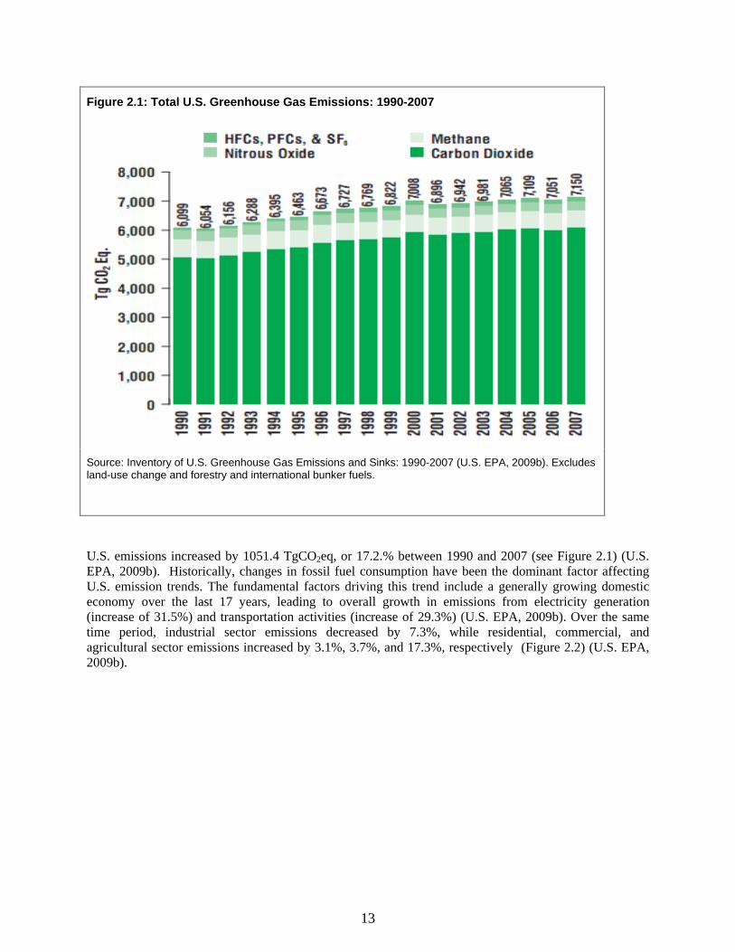
U.S. emissions increased by 1051.4 TgCO2eq, or 17.2.% between 1990 and 2007 (see Figure 2.1) (U.S. EPA, 2009b). Historically, changes in fossil fuel consumption have been the dominant factor affecting U.S. emission trends. The fundamental factors driving this trend include a generally growing domestic economy over the last 17 years, leading to overall growth in emissions from electricity generation (increase of 31.5%) and transportation activities (increase of 29.3%) (U.S. EPA, 2009b). Over the same time period, industrial sector emissions decreased by 7.3%, while residential, commercial, and agricultural sector emissions increased by 3.1%, 3.7%, and 17.3%, respectively (Figure 2.2) (U.S. EPA, 2009b).

Figure 2.1: Total U.S. Greenhouse Gas Emissions: 1990-2007

Source: Inventory of U.S. Greenhouse Gas Emissions and Sinks: 1990-2007 (U.S. EPA, 2009b). Excludes land-use change and forestry and international bunker fuels.

14

U.S. Emissions of Selected Aerosols and Ozone Precursors Aerosols are not GHGs but rather small, short-lived particles present in the atmosphere with widely varying size, concentration, and chemical composition. They can be directly emitted or formed in secondary reactions from emitted compounds. Aerosols are removed from the atmosphere primarily through cloud processing and wet deposition in precipitation, a mechanism that establishes average tropospheric aerosol atmospheric lifetimes at a week or less (CCSP, 2009a). Tropospheric ozone is a short-lived GHG produced largely by chemical reactions of precursor species in the atmosphere. Aerosols and tropospheric ozone precursors do not have widely accepted GWP or CO2 equivalent values but can still have significant impacts on regional and global climate. Four of the more important aerosols are sulfates, nitrates, organic carbon, and black carbon. Tropospheric ozone is not directly emitted but is a secondary product formed by atmospheric reactions from ozone precursors such as volatile organic compounds (VOCs) and nitrogen oxides (NOx). While some aerosols are directly emitted, others are formed through secondary reactions (for example, sulfates and nitrates can be formed by oxidation of sulfur dioxide [SO2] and NOx respectively), and their properties can change as they mix and react in the atmosphere. In the United States, these substances have been controlled under a number of local, state, and federal regulations over the last several decades, either directly, for SO2 by the Clean Air Act Amendments of 1990, among other legislation; or indirectly, for black and organic carbon as components of particulate matter (a criteria pollutant); for example through the 2007 Highway Diesel Rule or the National Ambient Air Quality (NAAQS) standards. The U.S. inventory does include SO2 emissions, which were 5.9 Tg of sulfur (TgS) in 2007, a reduction from 10.5 TgS in 1990 (U.S. EPA, 2009b) and 12 TgS in 1980 (CCSP 2009a). EPA estimates that 0.44 TgS per year (yr-1) of those emissions come from the transportation sector (U.S. EPA, 2009b). National inventories do not yet explicitly include black carbon or organic carbon: however, black carbon and organic carbon emissions can be derived from total fine particulate matter (PM2.5) emissions, which were estimated to be 5.0 Tg in 2005. In that year, ammonia emissions were 3.7 Tg, and of the ozone precursors, NOx emissions were estimated to be 18.5 Tg and VOC emissions were 16.8 Tg (U.S. EPA, 2009c). According to the EPA, U.S. emissions of SOx, NOx, direct particulates, and ozone precursors have decreased from 1990 to 2007 (U.S. EPA, 2008), and average concentrations of sulfates, nitrates, particulate matter, and ozone as measured at U.S. monitoring sites have all decreased between 1990 and 2007 (U.S. EPA, 2008).

Figure 2.2: U.S. GHG Emissions Allocated to Economic Sector

Source: Inventory of U.S. Greenhouse Gas Emissions and Sinks: 1990-2007 (U.S. EPA, 2009b). All GHGs. Excludes land use, land-use change and forestry, emissions from U.S. territories and international bunker fuels.

15

U.S. Greenhouse Gas Emissions From Source Categories Under Section 202(a) of the Clean Air Act Source categories under Section 202(a) of the Clean Air Act include passenger vehicles, light- and heavy-duty trucks, buses, motorcycles, and the cooling systems designed for passenger comfort, as well as auxiliary systems for refrigeration. In 2007, Section 202(a) source categories collectively were the second largest GHG-emitting sector within the United States (behind the electricity generating sector), emitting 1,649 TgCO2eq and representing 23% of total U.S. GHG emissions. Between 1990 and 2007, total GHG emissions from passenger cars decreased 2.6%, while emissions from light-duty trucks increased 59 percent, largely due to the increased use of sport-utility vehicles and other light-duty trucks. Total global emissions are estimated by summing emissions of the six GHGs, by country. The World Resources Institute compiles data from recognized national and international data sources in its Climate Analysis Indicators Tool (CAIT).16 Globally, total GHG emissions were 38,725.9 TgCO2eq in 2005, the most recent year for which data are available for all countries and all GHGs (WRI, 2009).17 This global total for the year 2005 represents an increase of about 26% from the 1990 global GHG emission total of 30,704.9 TgCO2eq (WRI, 2009). Excluding land use, land-use change, and forestry, U.S. emissions were 18% of the total year 2005 global emissions (see Figure 2.3) (WRI, 2009). Global Greenhouse Gas Emissions

Globally in 2005, Section 202(a) source category GHG emissions represented 28% of global transport GHG emissions and 4.3% of total global GHG emissions (Figure 2.3). The global transport sector was 15% of all global GHG emissions in 2005. If U.S. Section 202(a) source category GHG emissions were ranked against total GHG emissions for entire countries, U.S. Section 202(a) emissions would rank behind only China, the United States as a whole, Russia, and India, and would rank ahead of Japan, Brazil, Germany, and every other country in the world (Figure 2.3).

16 Primary data sources referenced in CAIT include the U.S. Department of Energy’s Carbon Dioxide Information Analysis Center, EPA, the International Energy Agency, and the National Institute for Public Health and the Environment, an internationally recognized source of non-CO2 data. 17 Source: WRI Climate Analysis and Indicators Tool. Available at http://cait.wri.org/.

Figure 2.3: Total GHG Emissions for 2005 by Country and for U.S. Section 202a Source Categories

0

1,000

2,000

3,000

4,000

5,000

6,000

7,000

8,000

China

U.S.A

Wor

ld T

rans

port

Russia

India

U.S. S

ectio

n 20

2(a)

Japa

n

Brazil

Ger

man

y

Canad

aU.K

.

Mex

ico

Indo

nesia Ira

n

Tg

CO

2eq

.

Source: WRI (2009). Available at http://cait.wri.org/. Excludes land use, land-use change and forestry, and international bunker fuels. More recent emission data are available for the United States and other individual countries, but 2005 is the most recent year for which data for all countries and all gases are available. Data accessed August 5, 2009. Refer to Appendix B for U.S. section 202a data and reference.

16

Further detail on these emissions can be found in Appendix B of this document. Global Emissions of Aerosols Inventories of anthropogenic aerosol emissions are not regularly reported in most national climate inventories, and the uncertainties in inventory estimates tend to be larger than for GHGs, ranging from 15% for sulfur emissions to a factor of two for black carbon (Forster et al., 2007). CCSP (2009a) provided estimates for global emissions of black carbon, organic matter, and sulfur in the year 2000: 7.7 Tg yr–1 of black carbon, 47 Tg yr–1 of particulate organic matter, and 112.6 Tg yr–1 of sulfur emissions (including SO2 and particulate sulfate). Historically, particle emissions were high due to lack of particulate controls and use of biofuels, but more recently technological controls have led to reductions in particulate emissions from coal burning. Therefore, over the past century, emissions of particulates did not grow as fast as CO2 emissions, as the latter are roughly proportional to total fuel use (CCSP, 2009a). 2(b) Lifetime of Greenhouse Gases in the Atmosphere Greenhouse gas concentrations in the atmosphere are a function of both the emissions of the GHGs and the effective lifetime of these gases. Each gas has a characteristic lifetime that is a function of the total atmospheric burden and the removal mechanism (i.e., sinks) for that gas. Each GHG has different interactions of each gas with the various available sinks, which include chemical reaction with the hydroxyl (OH) free radical or other highly reactive species, photolysis by sunlight, dissolution into the oceans, reactions on the surface, biological processes, or other mechanisms. According to the IPCC, the lifetime of the HFCs of industrial importance range from 1.4 to 270 years, the lifetime of N2O is 114 years, and the lifetime of the PFCs and SF6 range from 1,000 to 50,000 years (Forster et al., 2007). The lifetime of CH4 is more complicated: the atmospheric lifetime or residence time (the burden over the sink) is 8.7 years; however, emissions of CH4 lead to consumption of the available OH sink, thereby increasing the lifetime for the remaining CH4 in the atmosphere. Therefore, a “perturbation lifetime” of CH4 that accounts for this effect is used for most purposes, and the IPCC reports the perturbation lifetime to be 12 years (Denman et al., 2007). Carbon dioxide has a very different life cycle compared to the other GHGs, which have well-defined lifetimes. Instead, unlike the other gases, CO2 is not destroyed by chemical, photolytic, or other reaction mechanisms, but rather the carbon in CO2 cycles between different reservoirs in the atmosphere, ocean, land vegetation, soils, and sediments. There are large exchanges between these reservoirs, which are approximately balanced such that the net source or sink is near zero. Anthropogenic CO2 emissions released through the use of fossil fuel combustion and cement production from geologically stored carbon (e.g., coal, oil, and natural gas) that is hundreds of millions of years old, as well as anthropogenic CO2

emissions from land-use changes such as deforestation, perturb the atmospheric concentration of CO2 and the distribution of carbon within different reservoirs readjusts. Carbon cycle models indicate that for a pulse of CO2 emissions, given an equilibrium background, 50% of the atmospheric increase will disappear within 30 years, 30% within a few centuries, and the last 20% may remain in the atmosphere for thousands of years (Denman et al., 2007). Because it takes one to two years to mix the emissions of a species throughout the troposphere, gases that are chemically stable and persist in the atmosphere over time scales of decades to centuries or longer are referred to in the IPCC as “long-lived” or “well-mixed” gases.

17

2(c) Historic and Current Global Greenhouse Gas Concentrations Greenhouse gas concentrations in the atmosphere vary over very long time scales in response to natural influences such as geologic activity and temperature change associated with ice age cycles, but ice core data show nearly constant concentrations of CO2, CH4 and N2O over more than 10,000 years prior to the Industrial Revolution. However, since the Industrial Revolution, anthropogenic GHG emissions have resulted in substantial increases in the concentrations of GHGs in the atmosphere (IPCC, 2007d; NRC, 2001a). Carbon Dioxide (CO2) Carbon dioxide concentrations have increased substantially from pre-industrial levels (Figure 2.4). The long-term trends in the CO2 concentrations are as follows (NOAA, 2009c; Forster et al., 2007; Karl et al., 2009): The CO2 concentration has increased about 38% from a pre-industrial value of about 280 parts per

million (ppm) to 385 ppm (which is about 0.039% of the atmosphere by volume) in 200818. The present atmospheric concentration of CO2 exceeds by far the natural range over the last 800,000

years (172 to 300 ppm) as determined from ice cores (Karl et al., 2009). The annual CO2 concentration growth rate19 has been larger since 2000 (2000-2008 average: 1.9 ppm

per year), than it was over the previous 20 years (1980-1999 average: 1.5 ppm per year) or since the beginning of continuous direct atmospheric measurements at Mauna Loa (1959–1999 average: 1.3 ppm per year) although there is year-to-year variability.

Almost all of the increase in the CO2 concentration during the Industrial Era is due to anthropogenic emissions (Forster et al., 2007). Since the 1980s, about half of the anthropogenic emissions have been taken up by the terrestrial biosphere and the oceans, but observations demonstrate that these processes cannot remove all of the extra flux due to human activities. Historically, about half of the anthropogenic emissions have remained in the atmosphere. There is year-to-year variability in the fraction of fossil fuel emissions remaining in the atmosphere due to changes in land-atmosphere fluxes associated with El Niño Southern Oscillation (ENSO20) and events such as the eruption of Pinatubo (Forster et al., 2007). The rate of emission of CO2 currently exceeds its rate of removal, and the slow and incomplete removal implies that small to moderate reductions in its emissions would not result in stabilization of CO2 concentrations but rather would only reduce the rate of its growth in coming decades (Meehl et al., 2007).

18 The 2008 value is preliminary. 19 The estimated uncertainty in the global annual mean growth rate at marine surface sites is 0.1010 ppm/yr, in the Mauna Loa growth rate it is 0.11 ppm/yr. The 2000-2008 average rate of change at Mauna Loa is 2.0 ppm/yr. 20 ENSO describes the full range of the Southern Oscillation (a see-saw of atmospheric mass or pressure between the Pacific and Indo-Australian areas) that includes both sea surface temperature (SST) increases as well as SST decreases when compared to a long-term average. It has sometimes been used by scientists to relate only to the broader view of El Niño or the warm events, the warming of SSTs in the central and eastern equatorial Pacific. The acronym, ENSO, is composed of El Niño-Southern Oscillation, where El Niño is the oceanic component of the phenomenon, and the Southern Oscillation is the atmospheric component.

18

Methane (CH4) Methane concentrations have also risen substantially (Figure 2.4). The following trends in atmospheric methane have been observed according to the NOAA State of the Climate reports for 2007 and 2008 and IPCC (Horvitz, 2008; Peterson and Baringer, 2009; Forster et al., 2007): The global atmospheric concentration of

methane has increased from a pre-industrial value of about 715 parts per billion (ppb) to 1732 ppb in the early 1990s, and was 1782 ppb in 2007—a 149% increase from pre-industrial levels.

The atmospheric concentration of methane in 2007 exceeds by far the natural range of the last 650,000 years (320 to 790 ppb) as determined from ice cores (Jansen et al., 2007).

Growth rates declined between the early 1990s and mid-2000s. The reasons for the decrease in the atmospheric CH4 growth rate and the implications for future changes in its atmospheric burden are not well understood but are clearly related to the imbalances between CH4 sources and sinks.

The methane concentration grew 7.5 ppb between 2006 and 2007, driven by increased emissions in both the Arctic and tropical regions likely caused by high temperatures and precipitation in wetland regions, particularly in the Arctic. Analysis of carbon monoxide measurements suggests little contribution from enhanced biomass burning. Methane concentrations grew again in 2008, with most of the increase driven by the tropics, the first consecutive year-to-year increases since 1998. The observed increase in methane concentration is very likely due to anthropogenic activities, predominantly agriculture and fossil fuel use, but relative contributions from different source types are not well determined (Forster et al., 2007).

Figure 2.4: Atmospheric Concentrations of Carbon Dioxide, Methane and Nitrous Oxide over the Last 10,000 Years

Source: IPCC (2007d). Atmospheric concentrations of carbon dioxide, methane and nitrous oxide over the last 10,000 years (large panels) and since 1750 (inset panels). Measurements are shown from ice cores (symbols with different colors for different studies) and atmospheric samples (red lines). The corresponding radiative forcings (discussed in Section 2(e)) are shown on the right-hand axes of the large panels.

19

Nitrous Oxide (N2O) The N2O concentration has increased 23% from its pre-industrial value of 262 ppb (Figure 2.4) to 322 ppb in 2007 (Peterson and Baringer, 2009). The concentration has increased linearly by about 0.8 ppb yr–1 over the past few decades and is due primarily to human activities, particularly agriculture and associated land-use change (Forster et al., 2007). Ice core data show that the present atmospheric concentration of N2O exceeds levels measured in the ice core record of the past 650,000 years, with sufficient resolution to exclude a peak similar to the present for at least the past 16,000 years with very high confidence (Jansen et al., 2007). Fluorinated Gases The industrial fluorinated gases that serve as substitutes for chlorofluorocarbons (CFCs) and hydrochlorofluorocarbons (HCFCs), such as HFCs, PFCs, and SF6, have relatively low atmospheric concentrations. Concentrations of many of these gases increased by large factors (between 1.3 and 4.3) between 1998 and 2005. These gases are almost entirely anthropogenic in origin, although CF4, which contributes 20% of the total forcing due to anthropogenic increases in these gases, has a natural source that accounts for about one-half of its current atmospheric content (Forster et al., 2007). Ozone-depleting substances covered by the Montreal Protocol Chlorofluorocarbons and HCFCs are GHGs that are entirely anthropogenic in origin. Emissions of these gases have decreased due to their phase-out under the Montreal Protocol, and the atmospheric concentrations of CFC-11 and CFC-113 are now decreasing due to natural removal processes (Forster et al., 2007). Ice core and in situ data confirm that industrial sources are the cause of observed atmospheric increases in CFCs and HCFCs (Forster et al., 2007). Ozone (O3) Due to its short atmospheric life time, tropospheric ozone concentrations exhibit large spatial and temporal variability. Changes in tropospheric ozone also occur due to changes in transport of ozone across the tropopause (Forster et al., 2007). Relative to the other GHGs, there is less confidence in reproducing the changes in ozone associated with large changes in emissions or climate, and in the simulation of observed long-term trends in ozone concentrations over the 20th century (Forster et al., 2007). Aerosols (Sulfates, Nitrates, Black Carbon, and Organic Carbon Aerosols) On a global basis, aerosol mass derives predominantly from natural sources, mainly sea salt and dust. However, anthropogenic (manmade) aerosols, arising primarily from a variety of combustion sources, can dominate concentrations in and downwind of highly populated and industrialized regions and in areas of intense agricultural burning (CCSP, 2009a). Aerosol optical density trends observed in the satellite and surface-based data records suggest that since the mid-1990s, the amount of anthropogenic aerosol has decreased over North America and Europe, but has increased over parts of east and south Asia; on average, the atmospheric concentration of low-latitude smoke particles has increased, consistent with changes in emissions (CCSP, 2009a). Ice core data from Greenland and Northern Hemisphere mid-latitudes show a very likely rapid post-industrial era increase in sulfate concentrations above the preindustrial background, though in recent years, SO2 emissions have decreased globally and in many regions of the Northern Hemisphere. In general, the concentration, composition, and distribution of aerosols in the paleoclimate record are not as well known as the long-lived GHGs (Jansen et al., 2007).

20

Part III

Global and U.S. Observed and Projected Effects From Elevated Greenhouse Gas Concentrations

21

Section 3 Direct Effects of Elevated Greenhouse Gas Concentrations Carbon dioxide and other GHGs can have direct effects that are independent of their radiative forcing on climate (the primary effect discussed throughout this document). Such effects are described in the following sections. Effects on Human Health Current and projected ambient GHG concentrations remain well below published thresholds for any direct adverse health effects, such as respiratory or toxic effects. The literature supporting this conclusion is described in Appendix C. Effects on Plants and Carbon Dioxide Fertilization Carbon dioxide can have a stimulatory or fertilization effect on plant growth. There is debate and uncertainty about the sensitivity of crop yields to the direct effects of elevated CO2 levels. However, the IPCC (Easterling et al., 2007) confirmed the general conclusions from its previous Third Assessment Report in 2001 and concluded that elevated CO2 levels are expected to result in small beneficial effects on crop yields. Experimental research on crop responses to elevated CO2 through the FACE (Free Air CO2 Enrichment)21 experiments indicate that, at ambient CO2 concentrations of 550 ppm (approximately double the concentration from pre-industrial times) crop yields increase under unstressed conditions by 10 to 25% for C3 crops, and by 0 to 10% for C4 crops22 (medium confidence). Crop model simulations under elevated CO2 are consistent with these ranges (high confidence) (Easterling et al., 2007). High temperatures and ozone exposure, however, could significantly limit the direct stimulatory CO2 response (see also Section 8 on Air Quality and Section 9 on Food Production and Agriculture). Studies have demonstrated increases in CO2 effects water use and water use efficiency of plants. For example, elevated CO2 causes partial stomatal closure, which decreases conductance, and reduces loss of water vapor from leaves to the atmosphere (Hatfield et al., 2008). Interpolating the results from several studies indicates that it is very likely that an increase in CO2 concentration from 380 to 440 ppm will cause reductions in stomatal conductance on the order of 10% compared to today’s values (Hatfield et al., 2008). Elevated CO2 may affect forage quality for livestock, because it can increase the carbon-to-nitrogen ratio in forages, thus reducing the nutritional value of those grasses. This, in turn, can affect animal weight and performance. The decline under elevated CO2 of C4 grasses, however, which are less nutritious than C3 grasses, may compensate for the reduced protein (Hatfield et al., 2008). At much higher ambient CO2 concentrations, such as those areas exposed to natural CO2 outgassing due to volcanic activity, the main characteristic of long-term elevated CO2 zones at the surface is the lack of vegetation (IPCC, 2005). New CO2 releases into vegetated areas cause noticeable die-off. In those areas where significant impacts to vegetation have occurred, CO2 makes up about 20 to 95% of the soil gas, whereas normal soil gas usually contains about 0.2 to 4% CO2. Carbon dioxide concentrations above 5% may be dangerous for vegetation and as concentrations approach 20%, CO2 becomes phytotoxic. Carbon

21 http://www.bnl.gov/face/ 22 C3 and C4 refer to different carbon fixation pathways in plants during photosynthesis. C3 is the most common pathway, and C3 crops (e.g., wheat, soybeans, and rice) are more responsive to CO2 enrichment than C4 crops such as maize.

22

dioxide can cause death of plants through “root anoxia,” together with low oxygen concentration (IPCC, 2005). No projections show CO2 concentrations approaching these phytotoxic levels. As concentrations of atmospheric CO2 increase, more CO2 is absorbed at the surface of oceans, estuaries, streams, and lakes. Increases in the amount of dissolved CO2 and, for some species, bicarbonate ions (HCO3

-) present in aquatic environments will lead to higher rates of photosynthesis in submerged aquatic vegetation, similar to the fertilization effects of CO2 enrichment on most terrestrial plants, if other limiting factors do not offset the potential for enhanced productivity. A study cited in Nicholls et al., (2007) indicates algal growth may also respond positively to elevated dissolved inorganic carbon (DIC), though marine macroalgae do not appear to be limited by DIC levels. An increase in epiphytic or suspended algae would decrease light available to submerged aquatic vegetation and also increase the incidence of algal blooms that lower dissolved oxygen available to fish and shellfish (Nicholls et al., 2007). Ocean Acidification According to the IPCC (Fischlin et al., 2007) elevated CO2 concentrations are resulting in ocean acidification, which may affect marine ecosystems (medium confidence). This issue is discussed further in Sections 4h, 6b, and 14a.

23

Section 4 Radiative Forcing and Observed Climate Change This section focuses primarily on the more significant effects associated with GHGs, which is their heat-trapping ability (referred to as radiative forcing) that results in climate change. Observed climate change is reviewed, including changes in temperature, precipitation, and sea level rise, for the globe and the United States. Observed changes in climate-sensitive physical and biological systems are also addressed, as well as observed trends in extreme events. Sections 7 to 16 provide more specific information on the sectoral implications of both the observed changes described here and the projected changes described in Section 6. 4(a) Radiative Forcing Due to Greenhouse Gases and Other Factors This section describes radiative forcing and the factors that contribute to it. Radiative forcing is a measure of the change that a factor causes in altering the balance of incoming (solar) and outgoing (infrared and reflected shortwave) energy in the Earth-atmosphere system, and thus shows the relative importance of different factors in terms of their contribution to climate change. Positive forcing means the factor causes a warming effect, and negative forcing means the factor causes a cooling effect. Radiative forcing values presented here for GHGs and other factors come from the IPCC Fourth Assessment Report of Working Group I (IPCC, 2007a). These radiative forcing values are the result of global changes in atmospheric concentrations of GHGs (see Section 2(c) above) and other factors, and are therefore not the result of U.S. transportation emissions in isolation. All values are for the year 2005 relative to pre-industrial times in 1750; represent global averages; and are expressed in watts per square meter23 (W/m2). IPCC (2007d) concluded that the understanding of anthropogenic warming and cooling influences on climate has improved since the IPCC Third Assessment Report, leading to very high confidence24 that the global average net effect of human activities since 1750 has been one of warming, with a radiative forcing of +1.6 (+0.6 to +2.4) W/m2. Greenhouse gases have a positive forcing because they absorb and reradiate in all directions outgoing, infrared radiation that would otherwise directly escape into space. The combined radiative forcing due to the cumulative (i.e., 1750 to 2005) increase in atmospheric concentrations of CO2, CH4, and N2O is +2.30 W/m2 (with an uncertainty range of +2.07 to +2.53 W/m2) (see Figure 4.1). This positive radiative forcing, like the observed accumulation of these gases in the atmosphere, is primarily anthropogenic in origin. Furthermore, the IPCC (2007d) stated that the rate of increase in positive radiative forcing due to these three GHGs during the industrial era is “very likely to have been unprecedented in more than 10,000 years.” The positive radiative forcing due to CO2 is the largest (+1.66 ± 0.17 W/m2) (Figure 4.1) and has increased by 20% from 1995 to 2005, the largest change for any decade in at least the last 200 years. Methane is the second largest source of positive radiative forcing (+0.48 ± 0.05 W/m2). Nitrous oxide has a positive radiative forcing of +0.16 (±0.02) W/m2.

23 Watts per square meter is the standard metric unit for radiative and other energy fluxes. 24 According to IPCC terminology, “very high confidence” conveys a 9 out of 10 chance of being correct. See Box 1.2 for a full description of IPCC’s uncertainty terms.

24

The other three GHGs reported by the U.S. Inventory—HFCs, PFCs and SF6—have a total radiative forcing in 2005 of +0.017 (±0.002) W/m2, which is increasing by roughly 10% per year (Forster et al., 2007). The ozone-depleting substances covered under the Montreal Protocol (CFCs, HCFCs, and chlorocarbons) are also strong GHGs and, as a group, contributed +0.32 (±0.03) W/m2 to anthropogenic radiative forcing in 2005. Their radiative forcing peaked in 2003 and is now beginning to decline (Forster et al., 2007). The radiative forcing due to the destruction of stratospheric ozone by these gases is estimated to be –0.05 ± 0.10 W/m2 with a medium level of scientific understanding (Forster et al., 2007). In addition to the six main GHGs directly emitted by human activities and the gases covered by the Montreal Protocol, there are additional anthropogenic and natural factors that contribute to both positive and negative forcing.

Figure 4.1: Global Average Radiative Forcing (RF) Estimates and Ranges in 2005 for Anthropogenic GHG Emissions and Other Factors

Source: IPCC (2007d). Global average radiative forcing (RF) estimates and ranges in 2005 for anthropogenic carbon dioxide (CO2), methane (CH4), nitrous oxide (N2O) and other important factors, together with the typical geographical extent (spatial scale) of the forcing and the assessed level of scientific understanding (LOSU). The net anthropogenic radiative forcing and its range are also shown. These require summing asymmetric uncertainty estimates from the component terms, and cannot be obtained by simple addition. Additional forcing factors not included here are considered to have a very low LOSU. Volcanic aerosols contribute an additional natural forcing but are not included in this figure due to their episodic nature. The range for linear contrails does not include other possible effects of aviation on cloudiness.

25

With regard to climate change, ozone affects the radiative budget of the atmosphere through its interaction with both shortwave and longwave radiation (Forster et al., 2007). Tropospheric ozone changes caused by emissions of ozone-forming chemicals, or precursors (nitrogen oxides, carbon monoxide, and hydrocarbons including methane), contribute a positive forcing of +0.35 (+0.25 to +0.65) W/m2. As described in CCSP (2008d), robust model simulations project climate change will also increase the radiative forcing from ozone by increasing stratosphere-troposphere exchange and hence ozone near the tropopause where it is most important radiatively. Unlike the GHGs mentioned previously, tropospheric ozone is not as well-mixed in the global atmosphere because its atmospheric lifetime is on the order of days to months (versus decades to centuries for the well-mixed GHGs). Tropospheric ozone is a criteria air pollutant under the U.S. Clean Air Act. Emissions of ozone precursors and other substances also contribute to changes in levels of the reactive gas OH. OH is the major oxidizing chemical in the atmosphere, destroying significant quantities of many non-CO2 GHGs (e.g., CH4, HFCs, HCFCs, and ozone) thus influencing their chemical lifetimes and radiative forcing; it also plays an important role in the formation of sulfate, nitrate, and some organic aerosol species (Forster et al., 2007). Anthropogenic emissions of aerosols contribute to both positive and negative radiative forcing. Aerosols are non-gaseous substances other than water or ice that are suspended in the atmosphere and are either solid particles or liquid droplets. Most aerosols, such as sulfates (which are mainly the result of SO2 emissions from fossil fuel burning), exert a negative forcing or cooling effect, as they reflect and scatter incoming solar radiation. Some aerosols, such as black carbon, cause a positive forcing by absorbing incoming solar radiation. IPCC (2007d) estimated that the net effect of all anthropogenic increases in aerosols (primarily sulfate, organic carbon, black carbon, nitrate, and dust) produce a cooling effect, with a total direct radiative forcing of –0.5 (–0.9 to –0.1) W/m2 and an additional indirect cloud albedo (i.e., enhanced reflectivity)25 forcing of –0.7 (–1.8 to –0.3) W/m2. Understanding of these forcings has improved since the IPCC Third Assessment Report (IPCC, 2001c) but nevertheless remain the dominant uncertainty in radiative forcing (IPCC, 2007d). The direct radiative forcing of the individual aerosol species is less certain than the total direct aerosol radiative forcing. The estimates are: sulfate, -0.4 ( 0.2) W/m2; fossil fuel organic carbon, -0.05 (0.05) W/m2; fossil fuel black carbon, +0.2 (0.15) W/m2; biomass burning, +0.03 (0.12) W/m2; nitrate, -0.1 (0.1) W/m2; and mineral dust, -0.1 (0.2) W/m2. Including both fossil fuel and biomass burning sources, the total black carbon aerosol forcing is estimated to be 0.34 (0.09 to 0.59) W/m2. In addition, black carbon can cause another positive radiative forcing effect (+0.1 (0.0 to +0.2) W/m2) by decreasing the surface albedo of snow and ice, although scientific understanding of this forcing is low (Forster et al., 2007), with implications for Arctic and glacial melt. Also, according to the CCSP (2009a), since aerosol forcing is much more pronounced on regional scales than on the global scale because of the highly variable aerosol distributions, it would be insufficient or even misleading to place too much emphasis on the global average, with effects being dependent on both the location and timing of the emissions. Aerosols can alter the atmospheric circulation patterns and water cycles due to the manner in which aerosols can heat the atmosphere and cool the surface as well as to various cloud interactions (CCSP, 2009a). The total forcing associated with anthropogenic aerosols is less certain than that for GHGs, due to the indirect effects of aerosols, including cloud formation and albedo change.

25 In addition to directly reflecting solar radiation, aerosols cause an additional, indirect negative forcing effect by enhancing cloud albedo (a measure of reflectivity or brightness). This effect occurs because aerosols act as particles around which cloud droplets can form; an increase in the number of aerosol particles leads to a greater number of smaller cloud droplets, which leads to enhanced cloud albedo. Aerosols also influence cloud lifetime and precipitation, but no central estimates of these indirect forcing effects are estimated by IPCC. These aerosol indirect effects remain some of the biggest uncertainties of the climate forcing/feedback processes (CCSP, 2009a).

26

The radiative forcing from increases in stratospheric water vapor due to oxidation of anthropogenic increases in CH4 is estimated to be +0.07 ± 0.05 W/m2 (Forster et al., 2007). The level of scientific understanding is low because the contribution of CH4 to the corresponding vertical structure of the water vapor change near the tropopause is uncertain. Changes in surface albedo due to human-induced land cover changes exert a forcing of –0.2 (–0.4 to 0.0) W/m2. Changes in solar irradiance since 1750 are estimated to cause a radiative forcing of +0.12 (+0.06 to +0.30) W/m2. This estimate is less than half of the estimate given in IPCC’s Third Assessment Report (2001), with a low level of scientific understanding (Forster et al., 2007). Uncertainties remain large because of the lack of direct observations and incomplete understanding of solar variability mechanisms over long time scales. Empirical associations have been reported between solar-modulated cosmic ray ionization of the atmosphere and global average low-level cloud cover, but evidence for a systematic indirect solar effect remains ambiguous. The lack of a proven physical mechanism and the plausibility of other causal factors make the association between galactic cosmic ray-induced changes in aerosol and cloud formation controversial (Forster et al., 2007). Although water vapor is the most important and abundant GHG in the atmosphere, human activities produce only a very small direct increase in tropospheric water vapor (Karl et al., 2009). Irrigation and deforestation both have small, poorly understood effects on humidity, in opposite directions, and the IPCC concluded that radiative forcing from these sources of tropospheric water vapor is smaller than their non-radiative effects (such as evaporative cooling). Emissions of water vapor from combustion processes are significantly lower than emissions from land use; hence the absence of water vapor in Figure 4.1 (Forster et al., 2007). As temperatures increase, however, tropospheric water vapor concentrations also increase, representing a key positive feedback (e.g., one that enhances warming) but not a forcing of climate change (Solomon et al., 2007). Feedbacks are defined as processes in the climate system (such as a change in water vapor concentrations) that can either amplify or dampen the system’s initial response to radiative forcing changes (NRC, 2005). 4(b) Global Changes in Temperature Multiple lines of evidence lead to the robust conclusion that the climate system is warming. The IPCC (2007d) stated in its Fourth Assessment Report: “Warming of the climate system is unequivocal, as is now evident from observations of increases in global average air and ocean temperatures, widespread melting of snow and ice, and rising global average sea level.” This finding was reaffirmed in the U.S. Global Change Research Program’s June 2009 report Global Climate Change Impacts in the United States (Karl et al., 2009). Air temperature is a main property of climate and the most easily measured, directly observable, and geographically consistent indicator of climate change. The extent to which observed changes in global and continental temperature and other climate factors can be attributed to anthropogenic emissions of GHGs is addressed in Section 5. Global Surface Temperatures Surface temperature is calculated by processing data from thousands of worldwide observation sites on land and sea. Substantial gaps in data coverage remain, especially in the tropics and the Southern Hemisphere, particularly Antarctica, although data coverage has improved with time. These gaps are

27

largest in the 19th century and during the two world wars (Trenberth et al., 2007). The long-term mean temperatures are calculated by interpolating within areas with no measurements using the collected data available. Mears et al. (2006) caution: “For regions with either poor coverage or data gaps, trends in surface air temperature should be regarded with considerable caution, but do not have serious effects on the largest of scales as most of the variability is well sampled.” Biases may exist in surface temperatures due to changes in station exposure and instrumentation over land, or changes in measurement techniques by ships and buoys in the ocean. It is likely that these biases are largely random and therefore cancel out over large regions such as the globe or tropics (Wigley et al., 2006). Likewise, urban heat island effects are real but local, and have not biased the large-scale trends (Trenberth et al., 2007). However, it is conceivable that systematic changes in many station exposures of a similar kind may exist over the land during the last few decades. If such changes exist, they may lead to small amounts of spurious cooling or warming, even when the data are averaged over large land areas (Mears et al., 2006). The following trends in global surface temperatures were observed for the period 1850 to 2005, according to the IPCC (Trenberth et al., 2007): Global mean surface temperatures have risen by 1.3 0.3F (0.74 ± 0.18°C) when estimated by a

linear trend over the last 100 years (1906–2005) as shown by the magenta line in Figure 4.2. The warmest years in the instrumental record of global surface temperatures are 1998 and 2005, with 1998 ranking first in one estimate, but with 2005 slightly higher in the other two estimates. 2002 to 2004 are the third, fourth, and fifth warmest years in the series since 1850. Eleven of the last 12 years (1995 to 2006) – the exception being 1996 – rank among the 12 warmest years on record since 1850. Temperatures in 2006 were similar to the average of the past five years.

The warming has not been steady, as shown in Figure 4.2. Two periods of warming stand out: an

increase of 0.63F (0.35°C) that occurred from the 1910s to the 1940s and then a warming of about 0.99F (0.55°C) from the 1970s up to the end of 2006. In between those two periods (from the 1940s to the 1970s), temperatures leveled off or cooled slightly. The remainder of the past 150 years has included short periods of both cooling and warming. The rate of warming over the last 50 years is almost double that over the last 100 years 0.23 0.05F vs. 0.13 0.04F (0.13 ± 0.03°C vs. 0.07 ± 0.02°C) per decade.

Land regions have warmed at a faster rate than oceans. Warming has occurred in both land and

oceans and in both sea surface temperature (SST) and nighttime marine air temperature over the oceans. However, for the globe as a whole, surface air temperatures over land have risen at about double the ocean rate after 1979 (more than 0.49F [0.27°C] per decade vs. 0.23F [0.13°C] per decade), with the greatest warming during winter (December to February) and spring (March to May) in the Northern Hemisphere. Recent warming is strongly evident at all latitudes in SSTs over each of the oceans.

Average Arctic temperatures increased at almost twice the global average rate in the past 100 years.

Arctic temperatures have high decadal variability. A slightly longer warm period, almost as warm as the present, was also observed from the late 1920s to the early 1950s, but appears to have had a different spatial distribution than the recent warming.

28

Between 1901 and 2005, statistically significant warming was observed over most of the world’s

surface with the exception of an area south of Greenland and three smaller regions over the southeastern United States and parts of Bolivia and the Congo basin. The lack of significant warming at about 20% of the locations and the enhanced warming in other places, is likely to be a result of changes in atmospheric circulation. Warming is strongest over the continental interiors of Asia and northwestern North America and over some mid-latitude ocean regions of the Southern Hemisphere as well as southeastern Brazil.

Since 1979, warming has been strongest over western North America; northern Europe and China in

winter; Europe and northern and eastern Asia in spring; Europe and North Africa in summer; and northern North America, Greenland, and eastern Asia in autumn.

Box 4.1: Updated Global Surface Temperature Trends Through 2008 The global surface temperature trend analysis in IPCC (2007a) includes data through 2005 from the United Kingdom’s Hadley Centre (Hadley Centre, 2009), referred to as HadCRUT. Three additional years of data have become available since then (2006-2008) and two additional global surface temperature datasets are available for

Figure 4.2: Annual Global Mean Temperatures (black dots) with Linear Fits to the Data.

Source: Solomon et al. (2007). The left-hand axis shows temperature anomalies relative to the 1961 to 1990 average, and the right-hand axis shows estimated actual temperatures, both in Celsius. Linear trends are shown for the last 25 (yellow), 50 (orange), 100 (magenta), and 150 years (red). The smooth blue curve shows decadal variations with the decadal 90% error range shown as a pale blue band about that line. The total temperature increase from the period 1850 to 1899 to the period 2001 to 2005 is 1.37°F ± 0.34°F (0.76°C ± 0.19°C).

29

comparison. The updated HadCRUT dataset26 (which spans 1850-2008), NOAA’s Merged Land-Ocean Surface Temperature dataset27 (which spans 1880-2008) (NOAA, 2009a), and NASA’s Global Surface Temperature dataset28 (which spans 1880-2008), (NASA, 2009) all indicate:

Eight of the 10 warmest years on record have occurred since 2001 The 10 warmest years have all occurred in the past 12 years The 20 warmest years have all occurred since 1981

2008 was the ninth warmest year on record globally for the NOAA and NASA datasets and the 10th warmest year on record for the HadCRUT dataset. The warmest year on record was 2005 for the NOAA and NASA datasets and 1998 for the HadCRUT dataset. Because trends may be sensitive to the choice of start date in a time series, it is instructive to analyze trends when varying these dates. The following table shows warming trends29 starting in 1880 (when data is available across all three datasets) at 20 year intervals for all three datasets:

Period HadCRUT NOAA NASA 1880-2008 0.11°F (0.061C) /decade 0.10°F (0.056C) /decade 0.10°F (0.056C) /decade 1900-2008 0.13°F (0.072C) /decade 0.13°F (0.072C) /decade 0.12°F (0.067C) /decade 1920-2008 0.13°F (0.072C) /decade 0.12°F (0.067C) /decade 0.12°F (0.067C) /decade 1940-2008 0.15°F (0.083C) /decade 0.15°F (0.083C) /decade 0.14°F (0.078C) /decade 1960-2008 0.25°F (0.14C) /decade 0.24°F (0.13C) /decade 0.24°F (0.13C) /decade 1980-2008 0.29°F (0.16C) /decade 0.30°F (0.17C) /decade 0.29°F (0.16C) /decade

These trends show strong agreement among the three datasets, a conclusion also drawn in CCSP (2006), Trenberth et al. (2007), and the NOAA study, “State of the Climate in 2008” (Peterson and Baringer, 2009). The warming rate in the last 10 30-year periods (averaging about 0.30°F [0.17C] per decade) is the greatest in the observed record, followed closely by the warming rate (averaging about 0.25°F [0.14C] per decade) observed during a number of 30-year periods spanning the 1910s to the 1940s. Though most of the warmest years on record have occurred in the last decade in all available datasets, according to an analysis of the HadCRUT dataset in the “State of the Climate in 2008” report (Peterson and Baringer, 2009), the rate of warming has, for a short time, slowed. The temperature trend calculated for January 1999 to December 2008 was about +0.13 ± 0.13°F (+0.07 ± 0.07°C) per decade, which is less than the 0.32°F (0.18°C) per decade trend

recorded between 1979 and 2005 (or 0.30°F [0.17C] per decade for 1980 to 2008 as stated above). However, NOAA (NOAA, 2009a) and NASA (NASA, 2009) trends do not show the same marked slowdown for the 1999-2008 period. The NOAA trend was ~0.21°F (0.12C) per decade while the NASA trend was ~0.34°F (0.19C) per decade. The variability among datasets is a reflection of fewer data points and some differences in dataset methodologies. Analysis of trends for the years 2000, 2001, and 2002 through 2008 indicate a rather flat trend, with slight warming or cooling depending on choice of dataset and start date. It is important to recognize that year-to-year fluctuations in natural weather and climate patterns can produce a period that does not follow the long-term trend (Karl et al., 2009). Thus, each year will not necessarily be warmer than every year before it, though the long-term warming trend continues (Karl et al., 2009). For a discussion of how recent temperature trends relate to future climate projections, refer to Section 6b.

26 Downloadable from: http://cdiac.ornl.gov/ftp/trends/temp/jonescru/global.dat 27 Downloadable from: ftp://ftp.ncdc.noaa.gov/pub/data/anomalies/annual.land_ocean.90S.90N.df_1901-2000mean.dat 28 Downloadable from: http://data.giss.nasa.gov/gistemp/tabledata/GLB.Ts+dSST.txt 29 The trends in this table do not provide uncertainty estimates and are, therefore, approximate. In Trenberth et al. (2007), the uncertainty is given for these three datasets for different time periods in Table 3.3 and is about ±0.03°F ( 0.017C) for 1901-2005 and ±0.09°F ( 0.05C) for 1979-2005. These uncertainty estimates could reasonably be interpolated to the time series in this table.

30

Temperature trend analysis over Antarctica is complicated due to large regional and interannual variability and sparse data coverage. Recent studies and assessments have led to some different conclusions. Trenberth et al. (2007) indicate cooling over most of interior Antarctica and strong warming over the peninsula. However, the NOAA report State of the Climate in 2008 (Peterson and Baringer, 2009) refers to a recent study that finds Antarctic warming is much broader in spatial extent, extending to include West Antarctica. Alternatively, it refers to another study that indicates little change in near-surface temperatures during the past 50 years over most of the continent despite finding marked warming over the Antarctic Peninsula. Global Upper Air Temperatures Temperature measurements have also been made above the Earth's surface over the past 50 to 60 years using radiosondes (balloon-borne instruments) and for the past 28 years using satellites. These measurements support the analysis of trends and variability in the troposphere (surface to 6.2 to 10 mi [10 to 16 kilometers, km]) and stratosphere 6.2 to 31 mi [10 to 50 km] above the Earth's surface). The CCSP prepared a report that assessed temperature changes in the atmosphere, differences in the changes at various levels in the atmosphere, and an explanation of the causes of these changes and differences. It concluded (Wigley et al., 2006): “…the most recent versions of all available data sets show that both the surface and troposphere have warmed, while the stratosphere has cooled. These changes are in accord with our understanding of the effects of radiative forcing agents and with the results from model simulations.” The IPCC (Trenberth et al., 2007) reaffirmed the major conclusions of this CCSP report finding: New analyses of radiosondes and satellite measurements of lower- and mid-tropospheric temperature

show warming rates that are similar to those of the surface temperature record and are consistent within their respective uncertainties.

The satellite tropospheric temperature record is broadly consistent with surface temperature trends.

The range (due to different data sets) of global surface warming since 1979 is 0.29F (0.16°C) to 0.32F (0.18°C) per decade compared to 0.22F (0.12°C) to 0.34F (0.19°C) per decade for estimates of tropospheric temperatures measured by satellite.

Lower-tropospheric temperatures measured by radiosondes have slightly greater warming rates than

those at the surface over the period 1958 to 2005. The radiosonde record is markedly less spatially complete than the surface record and increasing evidence suggests that it is very likely that a number of records have a cooling bias, especially in the tropics.

Lower stratospheric temperatures have cooled since 1979. Estimates from adjusted radiosondes, satellites, and re-analyses are in qualitative agreement, suggesting a lower-stratospheric cooling of between 0.5F (0.3°C) and 1F (0.6°C) per decade since 1979. The global upper air temperature trend analysis in IPCC (2007a) described above includes data through 2005. Three additional years of data have become available since then (2006–2008). The addition of these three years does not significantly alter the above trends. For example, in NOAA (2009b) the satellite mid-tropospheric temperature trend computed for 1979–2008 ranges from +0.20 to 0.27F (+ 0.11°C to + 0.15°C) per decade compared to the estimate of +0.22 to +0.34F (+ 0.12°C to + 0.19°C) per decade given in IPCC (2007a). Combining the radiosonde and satellite records of the troposphere, the

31

State of the Climate in 2008 report estimates the trend is +0.261 0.04F (+0.145 ± 0.02°C) per decade for the period 1958–2008 with the range of the trends calculated from the various datasets (Peterson and Baringer, 2009). The report notes there is no indication of acceleration of the trend. As in the surface temperature data, the trend over the last seven to 10 years in these data is relatively flat, but this does not fundamentally alter the longer term warming signal. The 2008 annual average temperature of the lower stratosphere was similar to that of the last dozen years according to the State of the Climate in 2008 report (Peterson and Baringer, 2009). The report notes that globally the lower stratosphere has been about 2.7F (1.5°C) cooler over the past decade than in the 1960s when the radiosonde network began to offer reasonable global monitoring. It finds the general evolution of global lower stratospheric temperature is robustly captured in all available radiosonde (1958–present) and satellite (1979–present) datasets. However, the datasets differ in detail. For example, of those that cover 1979–2008, 2008 ranks as the coldest year in three, the second coldest in one, and the eighth coldest in another (Peterson and Baringer, 2009). Global Surface Temperatures Over the Last 2,000 Years Instrumental surface temperature records only began in the late 19th century, when a sufficiently large global network of measurements was in place to reliably compute global mean temperatures. To estimate temperatures further back in time, scientists analyze proxy evidence from sources such as tree rings, corals, ocean and lake sediments, cave deposits, ice cores, boreholes, glaciers, and documentary evidence. A longer temperature record can help place the 20th century warming into a historical context. NRC conducted a study to describe and assess the state of scientific efforts to reconstruct surface temperature records for the Earth over approximately the last 2,000 years and the implications of these efforts for understanding global climate change. It found (NRC, 2006b): Large-scale surface temperature reconstructions, as illustrated in Figure 4.3, yield a generally

consistent picture of temperature trends during the preceding millennium, including relatively warm conditions centered around 1000 A.D. (identified by some as the “Medieval Warm Period”) and a relatively cold period (or “Little Ice Age”) centered around 1700.

It can be said with a high level of confidence that global mean surface temperature was higher during

the last few decades of the 20th century than during any comparable period during the preceding four centuries. The observed warming in the instrumental record shown in Figure 4.2 supports this conclusion.

Less confidence can be placed in large-scale surface temperature reconstructions for the period from

900 to 1600 A.D. Presently available proxy evidence indicates that temperatures at many, but not all, individual locations were higher during the past 25 years than during any period of comparable length since 900 A.D. The uncertainties associated with reconstructing hemispheric mean or global mean temperatures from these data increase substantially backward in time through this period and are not yet fully quantified.

32

Very little confidence

can be assigned to statements concerning the hemispheric mean or global mean surface temperature prior to about 900 A.D. because of sparse data coverage and because the uncertainties associated with proxy data and the methods used to analyze and combine them are larger than during more recent time periods.

Considering this study and additional research, the IPCC (2007d) concluded: “Paleoclimatic information supports the interpretation that the warmth of the last half century is unusual in at least the previous 1,300 years.” However, like NRC (2006b), IPCC cautions that uncertainty is significant prior to 1600 (Jansen et al., 2007). 4(c) U.S. Changes in Temperature Like global mean temperatures, U.S. temperatures also warmed during the 20th and into the 21st century. According to NOAA (2009e) and data from NOAA30: U.S. average annual temperatures (for the contiguous United States or lower 48 states) are now

approximately 1.25°F (0.69°C) warmer than at the start of the 20th century, with an increased rate of warming over the past 30 years. The rate of warming for the entire period of record (1901–2008) is 0.13°F (0.072C) per decade while the rate of warming increased to 0.58°F (0.32°C) per decade for the period 1979–2008.

2005, 2006, and 2007 were exceptionally warm years (among the top 10 warmest on record), while

2008 was slightly warmer than average (the 39th warmest year on record), 0.2°F (0.1°C) above the 20th century (1901-2000) mean (though 0.06°F (0.035°C) below the 1971-2000 mean).

30 Data for contiguous U.S. temperature time series analysis obtained from NOAA’s National Climatic Data Center (NCDC). Data may be downloaded from: http://www.epa.gov/climatechange/endangerment/data.html (see file: us-temps-time-series-1901-2008-noaa.pdf).

Figure 4.3: Reconstructions of (Northern Hemisphere Average or Global Average) Surface Temperature Variations from Six Research Teams

Source: NRC (2006b). Reconstructions of (Northern Hemisphere average or global average) surface temperature variations from six research teams (in different color shades), along with the instrumental record of global average surface temperature (in black). Each curve illustrates a somewhat different history of temperature changes, with a range of uncertainties that tend to increase backward in time (as indicated by the shading).

33

The last 10 five-year periods (2004–2008, 2003–2007, 2002–2006, 2001–2005, 2000–2004, 1999–2003, 1998–2002, 1997–2001, 1996–2000, and 1995–1999), were the warmest five-year periods (i.e., pentads) in the period of record (since 1901), demonstrating the anomalous warmth of the last 15 years.

NASA’s U.S. temperature dataset31 for the lower 48 states indicates a somewhat lower warming trend (relative to NOAA) of 0.079°F (0.044C) per decade for the period 1901–2008. But this warming trend increases to 0.47°F (0.26C) per decade for the period 1979–2008 and the last eight five-year periods have been among the 10 warmest five-year periods on record. 1998 and 1934 are tied for the warmest year in NASA’s U.S. record. Over the past 50 years, Karl et al. (2009) report the U.S. average temperature has risen more than 2°F (1C) over the past 50 years resulting in longer warm seasons and shorter, less-intense cold seasons. Regional data33 analyzed from NOAA through 2008, as illustrated in Figure 4.4, indicate warming has occurred throughout most of the United States, with all but four of the 11 climate regions showing an increase of more than 1ºF (0.6C) since 1901 (NOAA, 2009d). As shown in Figure 4.4, the greatest temperature increase occurred in Alaska (for the period 1918–2008) and the Northeast (1.9°F [1.06C] and 2.0°F [1.1C] per century, respectively). The least warming occurred in the Southeast, where the trend was 0.26°F (0.14C) per century. Including all of North America in its assessment of regional temperatures, the IPCC (Field et al., 2007) stated: For the period 1955–2005, the greatest warming occurred in Alaska and northwestern Canada, with

substantial warming in the continental interior and modest warming in the southeastern United States and eastern Canada.

Spring and winter show the greatest changes in temperature and daily minimum (nighttime)

temperatures have warmed more than daily maximum (daytime) temperatures.

31 NASA U.S. temperature data may be downloaded from: http://data.giss.nasa.gov/gistemp/graphs/Fig.D.txt. 32 Data for U.S. temperature map obtained from NOAA’s NCDC. Data may be downloaded from: http://www.epa.gov/climatechange/endangerment/data.html (see file: us-temps-map-fig4-4-1901-2008-noaa.pdf). 33 Data for U.S. regional temperature time series analysis obtained from NOAA’s NCDC. Data may be downloaded from: http://www.epa.gov/climatechange/endangerment/data.html (see file: us-regional-temps-time-series-1901-2008-noaa.pdf).

Figure 4.4: Map of the United States, Depicting Regional U.S. Temperature Trends for the Period 1901 to 200832

Red shades indicate warming over the period and blue shades indicate cooling over the period.

34

4(d) Global Changes in Precipitation A consequence of rising temperature is increased evaporation, provided that adequate surface moisture is available (e.g., over the oceans and other moist surfaces). The average atmospheric water vapor content has increased since at least the 1980s over land and ocean, as well as in the upper troposphere (IPCC, 2007d). When evaporation increases, more water vapor is available for precipitation producing weather systems leading to precipitation increases in some areas. Conversely, enhanced evaporation and evapotranspiration from warming accelerates land surface drying and increases the potential incidence and severity of droughts in other areas. Observations show that changes are occurring in the amount, intensity, frequency, and type of precipitation. Cautioning that precipitation is highly variable spatially and temporally, and data are limited in some regions, the IPCC highlighted the following trends (Trenberth et al., 2007): Long-term trends from 1900 to 2005 have been observed in precipitation amount over many large

regions. Significantly increased precipitation has been observed in eastern parts of North and South America, northern Europe, and northern and central Asia.

Drying has been observed in northern Africa, southern Eurasia, Canada, and Alaska (Trenberth et al.,

2007). The IPCC notes the trend towards drying in northern Africa and the Sahel region, with a partial recovery since 1990, has been a common feature of climate in these regions in the paleoclimate record (Jansen et al., 2007).

For 1961–1990, rising temperature have generally resulted in rain rather than snow in locations and

seasons where climatological average temperatures were close to 32F (0°C). The trends described in the NOAA report State of the Climate in 2008 (Peterson and Baringer, 2009) are largely consistent with the IPCC. The NOAA report finds on a century time scale, most of the globe has trended towards wetter conditions, and particularly the northern high latitudes. But it also finds notable exceptions. A trend towards drier conditions is found over the tropics and some other locations. These include parts of southern Europe, most of Africa (while noting the drying trend over the Sahel reversed in 1989), southwestern Australia, and the west coast of South America. It highlights two regions that have become significantly drier over the past two decades: the southwestern United States and southeastern Australia. For information on changes in global precipitation extremes (heavy precipitation and drought), see Section 4(k).

35

4(e) U.S. Changes in Precipitation Data35 analyzed from NOAA show that over the contiguous United States, total annual precipitation increased at an average rate of 6.1% per century from 1901–2008, and about 5% over the last 50 years (Karl et al., 2009). As shown in Figure 4.5 displaying regional data36, the greatest increases in precipitation were in the East North Central climate region (9.6% per century), the Northeast (9.8% per century) and the South (10.5%). Precipitation increased in the Southeast by 1.3%, the Central United States by 7.2%, the West North Central by 4.0%, the Southwest by 3.7%, the West by 3.8%, and the Northwest by 4.1%. Outside the contiguous United States, Hawaii experienced a decrease of 5.4% per century (since records begin in 1905). Precipitation over Alaska (not shown due to limited data coverage) has a decreasing long-term trend, but with significant variability over time and space. Despite the overall national trend towards wetter conditions, a severe drought has affected the southwest United States from 1999 through 2008 (see Section 4(l)), which is indicative of significant variability in regional precipitation patterns over time and space. 4(f) Global Sea Level Rise and Ocean Heat Content Global Sea Level Rise There is strong evidence that global sea level gradually rose in the 20th century and is currently rising at an increased rate, after a period of little change between AD 0 and AD 1900 (IPCC, 2007a). According to Bindoff et al. (2007), there is high confidence that the rate of sea level rise increased between the mid-19th and mid-20th centuries. The average rate of sea level rise measured by tide gauges from 1961 to 2003 was 0.071 0.02 inch (0.18 0.05 cm) per year (Bindoff et al., 2007). The global average rate of sea level rise measured by satellite altimetry during 1993 to 2003 was 0.12 0.03 inch (0.31 0.07 cm) per year (Bindoff et al., 2007). Coastal tide gauge measurements confirm this observation. It is unclear whether the faster rate for 1993 to 2003 is a reflection of short-term variability

34 Data for U.S. precipitation map obtained from NOAA’s NCDC. Data may be downloaded from: http://www.epa.gov/climatechange/endangerment/data.html (see file: us-precip-map-fig4-5-1901-2008-noaa.pdf). 35 Data for contiguous U.S. precipitation time series analysis obtained from NOAA’s National Climatic Data Center. Data may be downloaded from: http://www.epa.gov/climatechange/endangerment/data.html (see file: us-precip-time-series-1901-2008-noaa.pdf). 36 Data for U.S. regional precipitation time series analysis obtained from NOAA’s National Climatic Data Center. Data may be downloaded from: http://www.epa.gov/climatechange/endangerment/data.html (see file: us-regional-precip-time-series-1901-2008-noaa.pdf).

Figure 4.5: Map of the United States, Depicting Precipitation Trends for the Contiguous United States 1901-2008 and Hawaii 1905-200834

Green shades indicate a trend toward wetter conditions over the period, and brown shades indicate a trend toward dryer conditions. No data are available for areas shaded white.

36

or an increase in the longer-term trend (Bindoff et al., 2007). The total 20th century sea level rise is estimated to be 6.7 2 inches (17 ± 5 (cm)) (Bindoff et al., 2007). Sources of uncertainty in measuring global average sea level rise include the adjustment for vertical land movements in tide gauge data and the proper accounting for instrumental bias and drifts in satellite altimetry data (Bindoff et al., 2007). Two major processes lead to changes in global mean sea level on decadal and longer time scales: i) thermal expansion, and ii) the exchange of water between oceans and other reservoirs (glaciers and ice caps, ice sheets, and other land water reservoirs). It is believed that on average, over the period from 1961 to 2003, thermal expansion contributed about one-quarter of the observed sea level rise, while melting of land ice accounted for less than half; the full magnitude of the observed sea level rise was not satisfactorily explained by the available data sets (Bindoff et al., 2007). During this period, global ocean temperature rose by 0.18F (0.10°C) from the surface to a depth of 2,300 ft (700 m), contributing an average of 0.016 0.004 inch (0.04 ± 0.01 cm) yr-1 to sea level rise (Bindoff et al., 2007). The contribution from ice was approximately 0.028 0.02 inch (0.07 ± 0.05 cm) yr-1 (Lemke et al., 2007). In recent years (1993–2003), during which the observing system has been much better, thermal expansion and melting of land ice each account for about half of the observed sea level rise, although there is some uncertainty in the estimates. Thermal expansion contributed about 0.063 0.02 inch (0.16 ± 0.05 cm) per year, reflecting a high rate of warming for the period relative to 1961 to 2003 (Bindoff et al., 2007). The total contribution from melting ice to sea level change between 1993 and 2003 ranged from 0.047 0.016 inch (0.12 ± 0.04 cm) per year. The rate increased over the 1993 to 2003 period primarily due to increasing losses from mountain glaciers and ice caps, from increasing surface melt on the Greenland Ice Sheet, and from faster flow of parts of the Greenland and Antarctic Ice Sheets (Lemke et al., 2007). Thermal expansion and exchanges of water between oceans and other reservoirs cause changes in the global mean as well as geographically non-uniform sea level change. Other factors influence changes at the regional scale, including changes in ocean circulation or atmospheric pressure, and geologic processes (Bindoff et al., 2007). Satellite measurements (for the period 1993–2003) provide unambiguous evidence of regional variability of sea level change (Bindoff et al., 2007). In some regions, rates of rise have been as much as several times the global mean, while sea level is falling in other regions. According to the IPCC (Bindoff et al., 2007), the largest sea level rise since 1992 has taken place in the western Pacific and eastern Indian oceans, while nearly all of the Atlantic Ocean shows sea level rise during the past decade with the rate of rise reaching a maximum (over 0.08 inch [0.2 cm] yr–1) in a band running east-northeast from the U.S. east coast. Sea level in the eastern Pacific and western Indian oceans has been falling. Ocean Heat Content The thermal expansion of sea water is an indicator of increasing ocean heat content. Ocean heat content is also a critical variable for detecting the effects of the observed increase in GHGs in the Earth’s atmosphere and for resolving the Earth’s overall energy balance (Bindoff et al., 2007). For the period 1955 to 2005, Bindoff et al. (2007) analyze multiple time series of ocean heat content and find an overall increase, while noting interannual and inter-decadal variations. NOAA’s report State of the Climate in 2008 (Peterson and Baringer, 2009), which incorporates data through 2008, finds “large” increases in global ocean heat content since the 1950s and notes that over the last several years, ocean heat content has reached consistently higher values than for all prior times in the record.

37

4(g) U.S. Sea Level Rise Sea level37 has been rising 0.08 to 0.12 inch yr-1 (0.2 to 0.3 cm yr-1) along most of the U.S. Atlantic and Gulf coasts, as seen in Figure 4.6. During the past 50 years, sea level has risen up to 8 inches (20 cm) or more along some coastal areas, and has fallen in other locations (Karl et al., 2009). The rate of sea level rise varies from about 0.36 inch per year (1 cm yr–1) along the Louisiana Coast (due to land sinking), to a drop of a few inches per decade in parts of Alaska (because land is rising). Records from the coast of California indicate that sea levels have risen almost 7.1 inches (18 cm) during the past century (California Energy Commission, 2006). According to the CCSP (2009b), in the Mid-Atlantic region from New York to North Carolina, tide-gauge observations indicate that relative sea level rise (the combination of global sea level rise and land subsidence) rates were higher than the global mean and generally ranged between 0.094 and 0.17 inch (0.24 and 0.44 cm) yr-1, or about 1 inch (2.54 cm) over the 20th century.

37 U.S. sea level data obtained from the Permanent Service for Mean Sea Level (http://www.pol.ac.uk/psmsl/) of the the Proudman Oceanographic Laboratory.

Figure 4.6: Relative Sea Level Changes on United States Coastlines, 1958 to 2008.

Source: Karl et al. (2009) Observed changes in relative sea level from 1958 to 2008 for locations on the United States coast.

38

Rosenzweig et al. (2007) document studies that find 75% of the shoreline, when the influence of spits, tidal inlets, and engineering structures is removed, is eroding along the U.S. East Coast probably due to sea level rise. They also cite studies reporting losses in coastal wetlands observed in Louisiana, the Mid-Atlantic region, and in parts of New England and New York, in spite of recent protective environmental regulations. 4(h) Global Ocean Acidification Ocean waters can absorb large amounts of CO2 from the atmosphere because when the gas dissolves in water it forms a weak acid, and the minerals dissolved in the ocean have created, over geologic time, a slightly alkaline ocean, with surface pH ranging from 7.9 to 8.25. The amount of carbon contained in the oceans has increased due to the elevated atmospheric pressure of CO2 from anthropogenic emissions (Denman et al., 2007). The IPCC estimates that the total inorganic carbon content of the oceans increased by 118 ± 19 gigatonnes of carbon (GtC) between 1750 and 1994 and continues to increase (Bindoff et al., 2007). This absorptive capacity of the oceans has resulted in atmospheric CO2 concentrations substantially lower than they otherwise would be. Since the beginning of the Industrial Revolution, global average sea surface pH has dropped by about 0.1 pH units, with the lowest decrease (0.06) in the tropics and subtropics, and the highest decrease (0.12) at high latitudes, consistent with the lower buffer capacity of the high latitudes compared to the low latitudes (Bindoff et al., 2007). This average pH decline of 0.1 pH unit corresponds to a 30% increase in the concentration of hydrogen ions (Denman et al., 2007). Ocean acidification is causing a series of cascading changes to the chemistry of ocean water, including a decrease in the saturation state of calcium carbonate. Marine calcifiers, such as corals, are dependent upon this mineral to form shells, skeletons, and other protective structures. Reduced availability of calcium carbonate can slow or even halt calcification rates in these organisms (Fischlin et al., 2007). The availability of carbonate is also important because it controls the maximum amount of CO2 that the ocean is able to absorb (Bindoff et al., 2007, p. 406). More information regarding ocean acidification projections and effects on marine ecosystems can be found in Sections 6(b) and 14(a), respectively. Ocean acidification is a direct consequence of fossil fuel CO2 emissions, which are also the main driver of the anticipated climate change (Denman et al., 2007). 4(i) Global Changes in Physical and Biological Systems Physical and biological systems on all continents and in most oceans are already being affected by recent climate changes, particularly regional temperature increases (very high confidence) (Rosenzweig et al., 2007). Climatic effects on human systems, although more difficult to discern due to adaptation and non-climatic drivers, are emerging (medium confidence) (Rosenzweig et al., 2007). The majority of evidence comes from mid- and high latitudes in the Northern Hemisphere, while documentation of observed changes in tropical regions and the Southern Hemisphere is sparse (Rosenzweig et al., 2007). Hence, the findings presented in this section apply generally to the globe but most directly to Europe and North America (including the United States) where these observational studies were conducted. The extent to which observed changes discussed here can be attributed to anthropogenic GHG emissions is discussed in Section 5. Cryosphere (Snow and Ice) Observations of the cryosphere (the “frozen” component of the climate system) have revealed changes in sea ice, glaciers and snow cover, freezing and thawing, and permafrost. The following physical changes have been observed:

39

Ice cover in the Arctic began to diminish in the late 19th century, and this shrinkage has accelerated during the last several decades. Shrinkages that were both similarly large and rapid have not been documented over at least the last few thousand years, although the paleoclimatic record is sufficiently sparse that similar events might have been missed (Alley et al., 2009). Total annual Arctic sea ice extent has been declining at the rate of 4.1% (193,000 mi2;~500,000 km2) per decade for the period 1979–2008 (NSIDC, 2009a). The latest data from NASA indicate Arctic sea ice set a record low in September 2007, 38% below the 1979–2007 average (NASA Goddard Space Flight Center, 2007). The extent of the sea ice loss between 1979 and 2007 can be seen in Figure 4.7. In September 2008, Arctic sea ice reached its second lowest extent on record (NASA Goddard Space Flight Center, 2008). In September 2009, Arctic sea ice reached its third lowest extent on record (NSIDC, 2009b). Figure 4.7: Arctic Sea Ice Concentrations Comparisons

1979 2007 Source: NASA (2007), Sea Ice Yearly Minimum 1979-2007. Available at: http://svs.gsfc.nasa.gov/vis/a000000/a003400/a003464/index.html. These two images, constructed from satellite data, compare arctic sea ice concentrations in September of 1979 and 2007 (Images courtesy of NASA). For the period 1979–2008, Antarctic sea ice underwent a not statistically significant increase of 0.9%

(~100,000 km2; 42,000 mi2) per decade (NSIDC, 2009a). The average sea ice thickness in the central Arctic has very likely decreased by up to 1 m from 1987

to 1997, based upon submarine-derived data. Model-based reconstructions support this finding, suggesting an Arctic-wide reduction of 24 to 35 inches (60 to 90 cm) over the same period (Lemke et al., 2007).

Mountain glaciers and snow cover have declined on average in both hemispheres with evidence of

acceleration in glacier decline in the last decade (Karl et al., 2009). o Though the studies cited by the IPCC (in Lemke et al., 2007) demonstrate widespread large-scale

retreat of glacier tongues since the 1800s and mass losses since the 1960s (when mass loss measurements began), IPCC cautions records of directly measured glacier mass balances are few, and that there is high spatial and temporal variability in glacier trends. For example, it discusses glaciers along the coast of Norway and in the New Zealand Alps that advanced in the 1990s and started to shrink around 2000. It also notes that whereas glaciers in the high mountains of Asia have generally shrunk, several high glaciers in the central Karakoram are reported to have advanced and/or thickened at their tongues.

o Northern hemisphere snow cover observed by satellite over the 1966–2005 period decreased in

every month except November and December, with a stepwise drop of 5% in the annual mean in the late 1980s (Lemke et al., 2007). The NOAA-led State of the Climate in 2008 report indicated the snow cover extent over the Northern Hemisphere in 2008 was 0.42 million square miles (1.1

40

million km2) less than the 39-year average, the fourth least extensive cover on record (Peterson and Baringer, 2009) In the Southern Hemisphere, the few long records or proxies mostly show either decreases or no changes in the past 40 years or more.

The freeze-up date for river and lake ice has occurred later at a rate of 5.8 ± 1.6 days per century,

averaged over available data for the Northern Hemisphere spanning the past 150 years. The breakup date has occurred earlier at a rate of 6.5 ± 1.2 days per century (Lemke et al., 2007).

Temperatures at the top of the permafrost layer have generally increased since the 1980s in the Arctic

(by up to 5F [3°C]). The permafrost base has been thawing at a rate ranging up to 1.6 inches (4 cm) yr-1 in Alaska since 1992 and 0.8 inch (2 cm) yr-1 on the Tibetan Plateau since the 1960s. The maximum area covered by seasonally frozen ground has decreased by 7% in the Northern Hemisphere since 1900, with a decrease in spring of up to 15% (Lemke et al., 2007).

There are additional effects related to changes in the cryosphere. Melting of highly reflective snow and ice reveals darker land and ocean surfaces, creating a positive feedback that increases absorption of the sun’s heat and further warms the planet. Increases in glacial melt and river runoff add more freshwater to the ocean, raising global sea level. Hydrosphere The term “hydrosphere” refers to the component of the climate system comprising liquid surface and subterranean water, such as rivers, lakes, and underground water. Several changes in these features have been observed, as summarized by the IPCC (Rosenzweig et al., 2007): Documented trends in severe droughts and heavy rains show that hydrological conditions are

becoming more intense in some regions. Globally, very dry areas (Palmer Drought Severity Index—PDSI—less than or equal to -3.0) have more than doubled since the 1970s due to a combination of ENSO events and surface warming. Very wet areas (PDSI greater than or equal to +3.0) declined by about 5% since the 1970s, with precipitation as the major contributing factor during the early 1980s and temperature more important thereafter. The areas of increasing wetness include the Northern Hemisphere high latitudes and equatorial regions.

Climate change signals related to increasing runoff and streamflow have been observed over the last

century in many regions, particularly in basins fed by glaciers, permafrost, and snowmelt. Evidence includes increases in average runoff of Arctic rivers in Eurasia, which has been at least partly correlated with climate warming, and earlier spring snowmelt and increase in winter base flow in North America and Eurasia due to enhanced seasonal snow melt associated with climate warming.

Freshwater lakes and rivers are experiencing increased water temperatures and changes in water

chemistry. Surface and deep lake-waters are warming, with advances and lengthening of periods of thermal stability in some cases associated with physical and chemical changes such as increases in salinity and suspended solids, and a decrease in nutrient content. Lake formation and subsequent disappearance in permafrost have been reported in the Arctic.

Changes in river discharge as well as in droughts and heavy rains in some regions indicate that

hydrological conditions have become more intense but significant trends in floods and in evaporation and evapotranspiration have not been detected globally. Some local trends in reduced ground water and lake levels have been reported, but studies have been unable to separate the effects of variations

41

in temperature and precipitation from the effects of human interventions such as ground water management (Rosenzweig et al., 2007).

Biosphere According to the IPCC, terrestrial ecosystems and marine and freshwater systems show that recent warming is strongly affecting natural biological systems (very high confidence) (Rosenzweig et al., 2007): The overwhelming majority of studies of regional climate effects on terrestrial species reveal

consistent responses to warming trends, including poleward and elevational range shifts of flora and fauna. Changes in abundance of certain species, including limited evidence of a few local disappearances, and changes in community composition over the last few decades have been attributed to climate change.

Responses of terrestrial species to warming across the Northern Hemisphere are well documented by

changes in the timing of growth stages, especially the earlier onset of spring events, migration, and lengthening of the growing season. Changes in phenology (the timing of annual phenomena of animal and plant life) include clear temperature-driven extension of the growing season by up to two weeks in the second half of the 20th century in mid- and high northern latitudes, mainly due to an earlier spring, but partly due also to a later autumn. Egg-laying dates have advanced in many bird species, and many small mammals have been found to come out of hibernation and to breed earlier in the spring now than they did a few decades ago.

Many observed changes in phenology and distribution of marine species have been associated with

rising water temperatures, as well as other climate-driven changes in salinity, oxygen levels, and circulation. For example, plankton has moved poleward by 10° latitude over a period of four decades in the North Atlantic. While there is increasing evidence for climate change impacts on coral reefs, discerning the impacts of climate-related stresses from other stresses (e.g., overfishing and pollution) is difficult. Warming of lakes and rivers is affecting abundance and productivity, community composition, phenology, distribution, and migration of freshwater species (high confidence).

4(j) U.S. Changes in Physical and Biological Systems Many of the global changes in physical and biological systems mentioned in Section 4(i) broadly apply to the United States. Some U.S.-specific changes in these systems cited in the IPCC’s Fourth Assessment Report are described in this subsection, as well as in Section 11(a) for physical systems related to water resources and Section 14(a) related to biological systems. Of all the observed changes to physical systems assessed by the IPCC (Rosenzweig et al., 2007) for North America (totaling 355), 94% of them were consistent with changes one would expect with average warming. Similar consistency was found between observed biological system changes and warming for North America (see discussion below under Biosphere). Furthermore, a CCSP (2008e) assessment reported that climate changes are very likely already affecting U.S. water resources, agriculture, land resources, and biodiversity as a result of climate variability and change. It noted that “[t]he number and frequency of forest fires and insect outbreaks are increasing in the interior West, the Southwest, and Alaska. Precipitation, streamflow, and stream temperatures are increasing in most of the continental United States. The western United States is experiencing reduced snowpack and earlier peaks in spring runoff. The growth of many crops and weeds is being stimulated. Migration of plant and animal species is changing the composition and structure of arid, polar, aquatic, coastal, and other ecosystems” (Backlund et al., 2008a)

42

Additional findings from this CCSP assessment along with results presented in IPCC’s Fourth Assessment Report are described in the following sections. Cryosphere (Snow and Ice) In North America, from 1915 to 2004, snow-covered area increased in November, December, and January due to increases in precipitation. However, snow cover decreased during the latter half of the 20th century, especially during the spring over western North America (Lemke et al., 2007). Eight-day shifts towards earlier melt since the mid-1960s were also observed in northern Alaska (Lemke et al., 2007). Consistent with these findings, Lettenmaier et al. (2008) note a trend toward reduced mountain snowpack, and earlier spring snowmelt runoff peaks across much of the western United States. The IPCC (Lemke et al., 2007) cites a study documenting glacier mass balance loss in the northwest United States and Alaska, with losses especially rapid in Alaska after the mid-1990s. Rosenzweig et al. (2007) refer to a study documenting evidence of present crustal uplift in response to recent glacier melting in Alaska. Hydrosphere Lettenmaier et al. (2008) document increases in U.S. streamflow during the second half of the 20th century consistent with increases in precipitation described in Section 4(e). Rosenzweig et al. (2007) indicate surface water temperatures have warmed by 0.4 to 4F (0.2 to 2°C) in lakes and rivers in North America since the 1960s. They also discuss evidence for an earlier occurrence of spring peak river flows and an increase in winter base flow in basins with important seasonal snow cover in North America. Biosphere The IPCC (Rosenzweig et al., 2007) assessed a multitude of studies that find changes in terrestrial ecosystems and marine and freshwater systems in North America. Of 455 biological observations assessed from these studies, 92% were consistent with the changes expected due to average warming. Backlund et al. (2008a) find: There has been a significant lengthening of the growing season and increase in net primary

productivity (NPP) in the higher latitudes of North America. Over the last 19 years, global satellite data indicate an earlier onset of spring across the temperate latitudes by 10 to 14 days.

In an analysis of 866 peer-reviewed papers exploring the ecological consequences of climate change,

nearly 60% of the 1,598 species studied exhibited shifts in their distributions and/or phenologies over the 20- and 140-year timeframe.

Subtropical and tropical corals in shallow waters have already suffered major bleaching events that

are clearly driven by increases in sea surface temperatures. In addition, Ryan et al. (2008) note that “[c]limate change has very likely increased the size and number of forest fires, insect outbreaks, and tree mortality in the interior West, the Southwest, and Alaska.”

43

4(k) Global Extreme Events Climate is defined not simply as average temperature and precipitation but also by the type, frequency, and intensity of extreme events. The IPCC documents observed changes in climate extremes related to temperature, precipitation, tropical cyclones, and sea level. The changes described apply generally to all parts of the globe, including the United States, although there are some regional and local exceptions due to patterns of natural climate variability. Current observations are summarized here, projected trends are covered in Section 6, and the sectoral impacts of these changes are covered as relevant in Sections 7 to 15. Temperature Widespread changes in extreme temperatures have been observed in the last 50 years. Cold days, cold nights, and frost have become less frequent, while hot days, hot nights, and heat waves have become more frequent (IPCC, 2007d). A widespread reduction in the number of frost days in mid-latitude regions, an increase in the number of warm extremes and a reduction in the number of daily cold extremes are observed in 70 to 75% of the land regions where data are available. The most marked changes are for cold nights (lowest 10%, based on 1961–1990), which have become rarer over the 1951–2003 period. Warm nights (highest 10%) have become more frequent. Heavy Precipitation and Drought Trenberth et al. (2007) note the following observed changes in drought and heavy precipitation events across the globe: More intense and longer droughts have been observed over wider areas since the 1970s, particularly

in the tropics and subtropics. Increased drying linked with higher temperatures and decreased precipitation has contributed to changes in drought. The regions where droughts have occurred seem to be determined largely by changes in sea surface temperatures (SSTs), especially in the tropics, through associated changes in the atmospheric circulation and precipitation. Decreased snowpack and snow cover have also been linked to droughts.

It is likely that there have been increases in the number of heavy precipitation events38 within many

land regions, even in those where there has been a reduction in total precipitation amount, consistent with a warming climate and observed significant increasing amounts of water vapor in the atmosphere. Increases have also been reported for rarer precipitation events (1-in-50-year return period), but only a few regions have sufficient data to assess such trends reliably (Trenberth et al., 2007).

Storms Trenberth et al (2007) find there has likely been a net increase in frequency and intensity of strong low-pressure systems (also known as mid-latitude storms and/or extratropical cyclones) over Northern Hemisphere land areas, as well as a poleward shift in track since about 1950. They caution, however, that detection of long-term changes in cyclone measures is hampered by incomplete and changing observing systems. They also note longer records for the northeastern Atlantic suggest that the recent extreme period may be similar in level to that of the late 19th century.

38 Heavy precipitation events refer to those in the 95th percentile of precipitation events.

44

The CCSP (2008i) report on extreme events, in its section on tropical cyclones (i.e., tropical storms and hurricanes), states that there have been spatially inhomogeneous increases in the power dissipation index, a measure of potential tropical cyclone destructiveness, over the last few decades (Kunkel et al., 2008). However, there remain reliability issues with historical data. Kunkel et al. (2008) refer to a study that was not able to corroborate the presence of upward intensity trends over the last two decades in ocean basins other than the North Atlantic. The report cautions that quantifying tropical cyclone variability is limited, sometimes seriously, by a large suite of problems with the historical record of tropical cyclone activity. Correspondingly, there is no clear trend in the annual numbers of tropical cyclones (IPCC, 2007d). The IPCC (2007a; Trenberth et al., 2007) concluded there is insufficient evidence to determine whether trends exist in small-scale phenomena such as thunderstorms, tornadoes, hail, lightning and dust-storms. High Sea Level Apart from non-climatic events such as tsunamis, extreme sea levels occur mainly in the form of storm surges generated by tropical or extra-tropical cyclones. There is evidence for an increase in extreme high sea level since 1975 based upon an analysis of 99th percentiles of hourly sea level at 141 stations over the globe (Bindoff et al., 2007). 4(l) U.S. Extreme Events Many of the global changes in extreme events mentioned in Section 4(k) broadly apply to the United States. Additionally, the U.S. CCSP (2008i) published a report that focused on changing climate extremes in the United States and North America. It concluded (Karl et al., 2008 in CCSP, 2008i):

Many extremes and their associated impacts are now changing. For example, in recent decades most of North America has been experiencing more unusually hot days and nights, fewer unusually cold days and nights, and fewer frost days. Heavy downpours have become more frequent and intense. Droughts are becoming more severe in some regions, though there are no clear trends for North America as a whole. The power and frequency of Atlantic hurricanes have increased substantially in recent decades, though North American mainland land-falling hurricanes do not appear to have increased over the past century. Outside the tropics, storm tracks are shifting northward and the strongest storms are becoming even stronger.

Many of these changes were also assessed in IPCC’s Fourth Assessment Report and are described in this subsection. Temperature The IPCC (Trenberth et al., 2007) cites North America regional studies that all show patterns of changes in temperature extremes consistent with a general warming. Since 1950, the annual percent of days exceeding the 90th, 95th, and 97.5 percentile thresholds for both maximum (hottest daytime highs) and minimum (warmest nighttime lows) temperature have increased when averaged over all of North America (Kunkel et al., 2008). Karl et al. (2008) conclude the number of heat waves (extended periods of extremely hot weather) has been increasing over the past 50 years. This conclusion is based on the following findings in Kunkel et al. (2008):

There was a highly statistically significant increase in the number of U.S. heat waves (defined as warm spells of 4 days in duration with mean temperature exceeding the threshold for a 1 in 10 year event) for the period 1960 to 2005

45

The annual number of warm spells (defined as at least three consecutive days above the 90th percentile threshold done separately for maximum and minimum temperature) averaged over all of North America has increased since 1950.

The heat waves of the 1930s remain the most severe in the U.S. historical record and suggest the intense drought of the period played a large role in the extreme heat by depleting soil moisture and reducing the moderating effects of evaporation.

Changes in cold extremes (days falling below the 10th, 5th, and 1st percentile threshold temperatures) show decreases, particularly since 1960 (Kunkel et al., 2008). Trenberth et al. (2007) cite a study finding intense warming of the lowest daily minimum temperatures over western and central North America. Trenberth et al. (2007) caution the observed changes of the tails of the temperature distributions are often more complicated than a simple shift of the entire distribution would suggest. Kunkel et al. (2008) find some evidence of a downward linear trend in cold waves (extended periods of cold) for the period 1895-2005, but note the trend is not statistically significant, largely owing to multi-decadal variabilty. But they find the very recent period from 1998-2007 exhibited fewer severe cold snaps than any other 10-year period in the historical record dating back to 1895. Kunkel et al. (2008) also indicate a decrease in frost days and a lengthening of the frost-free season over the past century. Heavy Precipitation and Drought In the contiguous United States, Trenberth et al. (2007) cite studies finding statistically significant increases in heavy precipitation (the heaviest 5%) and very heavy precipitation (the heaviest 1%) of 14 and 20%, respectively. The increase in the frequency and intensity of heavy downpours was responsible for most of the observed increase in overall precipitation (see Section 4e) during the last 50 years (Karl et al., 2009). Much of the increase in heavy precipitation occurred during the last three decades of the 20th century and is most apparent over the eastern parts of the country (Trenberth et al., 2007; Karl et al., 2009).). There is also evidence from Europe and the United States that the relative increase in precipitation extremes is larger than the increase in mean precipitation (Trenberth et al., 2007). In fact, Karl et al. report there has been little change in the frequency of light and moderate precipitation during the past 30 years. Lettenmaier et al. (2008) state that “[w]ith respect to drought, consistent with streamflow and precipitation observations, most of the continental United States experienced reductions in drought severity and duration over the 20th century. However, there is some indication of increased drought severity and duration in the western and southwestern United States….” For the past 50 years, Dole et al. (2008) conclude: “It is unlikely that a systematic change has occurred in either the frequency or area coverage of severe drought over the contiguous United States from the mid-twentieth century to the present." Diminishing snow pack and subsequent reductions in soil moisture appear to be factors in recent drought conditions in the western United States (Trenberth et al., 2007). This drought has also been attributed to changes in atmospheric circulation associated with warming of the western tropical Pacific and Indian oceans as well as multidecadal fluctuations (Trenberth et al., 2007). Jansen et al. (2007) find (based on paleoclimate studies) that there have been periods over the past 2,000 years during which drought in North America was "more frequent, longer and/or geographically more extensive ... than during the 20th century." They indicate some evidence suggests droughts were particularly extensive, severe, and frequent during intervals characterized by warmer than average summer temperatures in the Northern Hemisphere.

46

Storms Karl et al. (2008) indicate a northward shift in the tracks of strong low-pressure systems (also known as mid-latitude storms and/or extratropical cyclones) in both the North Atlantic and North Pacific over the past fifty years with increases in storm intensity noted in the Pacific (data inconclusive in the Atlantic). Correspondingly, they also find northward shift in snow storm occurrence, which is also consistent with the warming temperatures and a decrease in snow cover extent over the United States. Assessing trends in tropical cyclone (i.e., tropical storms and/or hurricanes) frequency and/or intensity is complicated by uncertainties in the observational record. Confidence in the tropical storm and hurricane record increases after 1900 and is greatest during the satellite era, from 1965 to present (Karl et al., 2009). IPCC (2007d) and Karl et al. (2009) report observational evidence of an increase in intense tropical cyclone activity in the North Atlantic (where cyclones develop that affect the U.S. East and Gulf Coasts) since about 1970, correlated with increases of tropical sea surface temperatures of nearly 2ºF (1C) in the main Atlantic hurricane development region (Karl et al., 2009). The strongest hurricanes (Category 4 and 5) have, in particular, increased in intensity (Karl et al., 2009). The total number of Atlantic hurricanes and strongest hurricanes observed from 1881 through 2008 shows multi-decade periods of above-average activity in the 1800s, the mid-1900s, and since 1995 (Karl et al., 2009). During this period, there has been little change in the total number of land-falling hurricanes (Karl et al., 2009). As in hurricanes, there are significant uncertainties in assessing long-term trends in thunderstorms and tornadoes due to changing observing systems. Kunkel et al. (2008) conclude: "There is no evidence for a change in the severity of tornadoes and severe thunderstorms, and the large changes in the overall number of reports make it impossible to detect if meteorological changes have occurred." High Sea Level Studies of the longest records of extremes in sea level are restricted to a small number of locations. Consistent with global changes, U.S.-based studies document increases in extreme sea level closely following the rise in mean sea level (Bindoff et al., 2007).

47

Section 5 Attribution of Observed Climate Change to Anthropogenic Greenhouse Gas Emissions at the Global and Continental Scale This section addresses the extent to which observed climate change at the global and continental or national scale (described in Section 4) can be attributed to global anthropogenic emissions of GHGs. Section 2 describes the share of the U.S. transportation sector to U.S. and global anthropogenic emissions of GHGs, and the resultant share of U.S. transportation emissions to global increases in atmospheric concentrations of GHGs. Evidence of the effect of anthropogenic GHG emissions on the climate system, as well as climate-sensitive systems and sectors, has increased over the last 15 years or so and even since the previous IPCC assessment published in 2001. The evidence in the recent IPCC Fourth Assessment Report (IPCC, 2007a) is based on analyses of global- and continental-scale temperature increases, changes in other climate variables and physical and biological systems, and the radiative forcing caused by anthropogenic versus natural factors. 5(a) Attribution of Observed Climate Change to Anthropogenic Emissions The attribution of observed climate change to anthropogenic activities is based on multiple lines of evidence. The first line of evidence arises from the basic physical understanding of the effects of changing concentrations of GHGs, natural factors, and other human impacts on the climate system. The second line of evidence arises from indirect, historical estimates of past climate changes that suggest that the changes in global surface temperature over the last several decades are unusual (Karl et al, 2009). The third line of evidence arises from the use of computer-based climate models to simulate the likely patterns of response of the climate system to different forcing mechanisms (both natural and anthropogenic). Confidence in these models comes from their foundation in accepted physical principles and from their ability to reproduce observed features of current climate and past climate changes (IPCC, 2007a). For additional discussion on the strengths and limitations of models, see Section 6(b). Attribution studies evaluate whether observed changes are consistent with quantitative responses to different forcings (from GHGs, aerosols, and natural forcings such as changes solar intensity) represented in well-tested models and are not consistent with alternative physically plausible explanations. Studies to detect climate change and attribute its causes using patterns of observed temperature change show clear evidence of human influences on the climate system (Karl et al., 2006). Discernible human influences extend to additional aspects of climate including ocean warming, continental-average temperatures, temperature extremes, and wind patterns (Hegerl et al., 2007). Temperature IPCC statements on the linkage between GHGs and temperatures have strengthened since the organization’s early assessments (Solomon et al., 2007). The IPCC’s First Assessment Report in 1990 contained little observational evidence of a detectable anthropogenic influence on climate (IPCC, 1990). In its Second Assessment Report in 1995, the IPCC stated the balance of evidence suggests a discernible human influence on the climate of the 20th century (IPCC, 1996). The Third Assessment Report in 2001 concluded that most of the observed warming over the last 50 years is likely to have been due to the increase in GHG concentrations (IPCC, 2001b). The conclusion in IPCC’s 2007 Fourth Assessment Report (2007b) is the strongest yet:

48

Most of the observed increase in global average temperatures since the mid-20th century is very likely39 due to the observed increase in anthropogenic GHG concentrations.

The IPCC (Hegerl et al., 2007) finds that anthropogenic GHG emissions were one of the influences contributing to temperature rise during the early part of the 20th century along with increasing solar output and a relative lack of volcanic activity. During the 1950s and 1960s, when temperature leveled off, increases in aerosols from fossil fuels and other sources are thought to have cooled the planet. For example, the eruption of Mt. Agung in 1963 put large quantities of reflective dust into the atmosphere. The rapid warming since the 1970s has occurred in a period when the increase in GHGs has dominated over all other factors (Hegerl et al., 2007). The increased confidence in the GHG contribution to the observed warming results from (Hegerl. et al., 2007): An expanded and improved range of observations allowing attribution of warming to be more fully

addressed jointly with other changes in the climate system. Improvements in the simulation of many aspects of present mean climate and its variability on

seasonal to inter-decadal time scales. More detailed representations of processes related to aerosol and other forcings in models. Simulations of 20th-century climate change that use many more models and much more complete

anthropogenic and natural forcings. Multi-model ensembles that increase confidence in attribution results by providing an improved

representation of model uncertainty. Box 5.1: The Relationship Between GHG Concentrations and Temperature Over Geologic Time and Implications for Attribution of Recent Global Temperature Trends Direct and proxy measurements of past changes in biological, chemical, and physical indicators provide a means of reconstructing key aspects of past climates. These measurements show that past climates have been both warmer and colder than present, and that warmer periods have generally coincided with high atmospheric CO2 levels (Jansen et al., 2007). While sources of uncertainty including inexact age models and possible seasonal biases remain a factor in paleoclimatic studies, recent methodological advances in, for example, multi-proxy approaches have led to increasingly confident reconstructions (Jansen et al., 2007). Climate reconstructions reaching back in time beyond the reach of ice cores (i.e., prior to about one million years ago) are uncertain, but generally verify that warmer climates are to be expected with increased GHG concentrations (Jansen et al., 2007). Jansen et al. (2007) report that the major expansion of Antarctic glaciations starting around 35 to 40 million years ago (Ma) was likely a response, in part, to declining atmospheric CO2, and that the major glaciations around 300 Ma likely coincided with low CO2 concentrations relative to the surrounding periods. The mid-Pliocene (about 3.3 to 3.0 Ma) is the most recent time in Earth’s history when global mean temperatures were substantially warmer than present for a prolonged period. Temperatures for mid-Pliocene are estimated by General Circulation Models (GCMs) to have been about 4 to 5F (2 to 3C) above pre-industrial levels (Jansen et al., 2007). The ice core record extends for approximately 800,000 years and allows for higher-confidence assessments compared to the more distant past. According to the IPCC (Jansen et al., 2007), “The ice core record indicates that GHG co-varied with Antarctic temperature over glacial-interglacial time scales, suggesting a close link between natural atmospheric GHG concentrations and temperature.” Evidence strongly suggests that the timing of glacial-interglacial periods are paced by the variations in the orbit of the earth; however, the large response of the climate system implies a strong positive amplification of the initial orbital forcing (Jansen et al., 2007). Jansen et al. (2007)

39 According to IPCC terminology, “very likely” conveys a 90 to 99% probability of occurrence. See Box 1.2 for a full description of IPCC’s uncertainty terms.

49

conclude: “It is very likely that glacial-interglacial CO2 variations have strongly amplified climate variations, but it is unlikely that CO2 variations have triggered the end of glacial periods. Antarctic temperatures started to rise several centuries before atmospheric CO2 during past glacial terminations.” CO2 (and other GHG) changes over glacial to interglacial transitions, therefore, contribute to, but do not initiate, the temperature changes seen. A variety of proxy records provide temporal and spatial information concerning climate change during the current interglacial, the Holocene, which began approximately 11.6 thousand years ago. Jansen et al. (2007) find evidence for local multi-centennial periods warmer than the last decades by up to several degrees in the early to mid-Holocene, but note that these local warm periods were very likely not globally synchronous and that the tendency for high-latitude summer temperature maxima to occur early in the Holocene (8,000-10,000 years ago) points to a direct influence of orbital forcing on temperature, rainfall, and sea ice extent. According to the IPCC (Jansen et al., 2007), current data limitations limit the ability to determine if there were multi-decadal periods of global warmth comparable to the last half of the 20th century prior to about 1,000 years ago. The IPCC (Hegerl et al., 2007) reports that analyses of paleoclimate have increased confidence in the role of external influences on climate, and that key features of past climates have been reproduced by climate models using boundary conditions and radiative forcing for those periods. Climate model simulations by the IPCC, shown in Figure 5.1, suggest natural forcings alone cannot explain the observed warming (for the globe, the global land and global ocean). The observed warming can only be reproduced with models that contain both natural and anthropogenic forcings.

Additional evidence documented in the IPCC report supports its statement linking warming to increasing concentrations of GHGs (Hegerl et al., 2007): Warming of the climate system has been detected in changes of surface and atmospheric

temperatures, in the upper several hundred meters of the ocean (as evident by the observed increase in ocean heat content, see Section 4(f)), and in contributions to sea level rise. Attribution studies have established anthropogenic contributions to all of these changes.

Figure 5.1: Comparison of Observed Global-Scale Changes in Surface Temperature with Results Simulated by Climate Models Using Natural and Anthropogenic Forcings

Source: IPCC (2007d). Decadal averages of observations are shown for the period 1906 to 2005 (black line) plotted against the center of the decade and relative to the corresponding average for 1901to1950. Lines are dashed where spatial coverage is less than 50%. Blue shaded bands show the 5 to 95% range for 19 simulations from five climate models to using only the natural forcings due to solar activity and volcanoes. Red shaded bands show the 5–95% range for 58 simulations from 14 climate models using both natural and anthropogenic forcings.

50

Analyses of paleoclimate data have increased confidence in the role of external influences on climate.

Coupled climate models used to predict future climate have been used to reproduce key features of past climates using boundary conditions and radiative forcing for those periods.

The IPCC states that it is very unlikely that the global pattern of warming observed during the past half century is due to only known natural external causes (solar activity and volcanoes) since the warming occurred in both the atmosphere and ocean and took place when natural external forcing factors would likely have produced cooling (Hegerl et al., 2007). It also states GHG forcing alone would likely have resulted in warming greater than observed if there had not been an offsetting cooling effect from aerosols and natural forcings during the past half century (Hegerl et al., 2007). Solomon et al. (2007) and Karl et al. (2009) indicate the sum of solar and volcanic forcing in the past half century would likely have produced cooling, not warming. Not only has an anthropogenic signal been detected for the surface temperatures, but evidence has also accumulated of an anthropogenic influence through the vertical profile of the atmosphere. Fingerprint studies40 have identified GHG and sulfate aerosol signals in observed surface temperature records, a stratospheric ozone depletion signal in stratospheric temperatures, and the combined effects of these forcing agents in the vertical structure of atmospheric temperature changes (Karl et al., 2006). Karl et al. (2009) state that more recent studies have also found human fingerprints in the patterns of change in Arctic and Antarctic temperatures. However, an important inconsistency may have been identified in the tropics. In the tropics, most observational data sets show more warming at the surface than in the troposphere, while almost all model simulations have larger warming aloft than at the surface (Karl et al., 2006). Karl et al. (2009) state that when uncertainties in models and observations are properly accounted for, newer observational data sets are in agreement with climate model results. The IPCC states that the substantial anthropogenic contribution to surface temperature increases likely applies to every continent except Antarctica (which has insufficient observational coverage to make an assessment) since the middle of the 20th century (Hegerl. et al., 2007). However, newer research led the USGCRP (Karl et al., 2009) to conclude that there are human fingerprints in the pattern of changes in Antarctic surface temperatures. Figure 5.2 indicates North America’s observed temperatures over the last century can only be reproduced using model simulations containing both natural and anthropogenic forcings. In the CCSP (2008g) report Reanalysis of Historical Climate Data for Key Atmospheric Features: Implications for Attribution of Causes of Observed Change, Dole et al. (2008) find that for North America “more than half of this warming [for the period 1951–2006] is likely the result of human-caused GHG forcing of climate change.”

40 Fingerprint studies use rigorous statistical methods to compare the patterns of observed temperature changes with model expectations and determine whether or not similarities could have occurred by chance. Linear trend comparisons are less powerful than fingerprint analyses for studying cause-effect relationships but can highlight important differences and similarities between models and observations (as in Figures 5.1 and 5.2).

51

Temperature extremes have also likely been influenced by anthropogenic forcing. Many indicators of climate extremes, including the annual numbers of frost days, warm and cold days, and warm and cold nights, show changes that are consistent with warming (Hegerl et al., 2007). An anthropogenic influence has been detected in some of these indices, and there is evidence that anthropogenic forcing may have substantially increased the risk of extremely warm summer conditions regionally, such as the 2003 European heat wave (Hegerl et al., 2007). Karl et al. (2008) conclude the increase in human-induced emissions of GHGs is estimated to have substantially increased the risk of a very hot year in the United States, such as that experienced in 2006. They add that other aspects of observed increases in temperature extremes, such as changes in warm nights and frost days, have been linked to human influences. The IPCC (Hegerl et al., 2007) cautions that difficulties remain in attributing temperature changes on smaller than continental scales and over time scales of less than 50 years. It states that attribution at these scales, with limited exceptions, has not yet been established. It further explains (Hegerl et al., 2007):

Averaging over smaller regions reduces the natural variability less than does averaging over large regions, making it more difficult to distinguish between changes expected from different external forcings, or between external forcing and variability. In addition, temperature changes associated with some modes of variability are poorly simulated by models in some regions and seasons. Furthermore, the small-scale details of external forcing, and the response simulated by models are less credible than large-scale features.

Changes arising from internally generated variations in the climate system can influence surface and atmospheric temperatures substantially; however, climate models indicate that global-mean unforced variations on multidecadal timescales are likely to be smaller than the 20th century global-mean increase in surface temperature (Karl et al., 2006). The IPCC reports that global mean and hemispheric scale temperatures on multi-decadal time scales are largely controlled by external forcing (Hegerl et al., 2007).

Figure 5.2: Comparison of Observed North American Changes in Surface Temperature with Results Simulated by Climate Models Using Natural and Anthropogenic Forcings

Source: Hegerl et al. (2007). Decadal averages of observations are shown for the period 1906 to 2005 (black line) plotted against the center of the decade and relative to the corresponding average for 1901 to1950. Lines are dashed where spatial coverage is less than 50%. Blue shaded bands show the 5 to 95% range for 19 simulations from five climate models using only the natural forcings due to solar activity and volcanoes. Red shaded bands show the 5 to 95% range for 58 simulations from 14 climate models using both natural and anthropogenic forcings.

52

Hegerl et al. (2007) note that “many observed changes in surface and free atmospheric temperature, ocean temperature, and sea ice extent, and some large-scale changes in the atmospheric circulation over the 20th century are distinct from internal variability and consistent with the expected response to anthropogenic forcing.” Additional Climate Variables There is evidence of anthropogenic influence in other parts of the climate system. The IPCC and CCSP noted the following examples: Anthropogenic forcing has likely contributed to the recent decreases in Arctic sea ice extent while

noting large-scale modes of variability contribute to interannual variations in ice formation (Hegerl et al., 2007). Karl et al. (2009) also state year-to-year changes in sea ice extent are influenced by natural variations but add that the observed decline in Arctic sea ice has been more rapid than projected by climate models, and clear linkages between rising GHG concentrations and declines in Arctic sea ice have been identified.

It is very likely that the response to anthropogenic forcing contributed to sea level rise during the

latter half of the 20th century. Models including anthropogenic and natural forcing simulate the observed thermal expansion since 1961 reasonably well. Anthropogenic forcing dominates the surface temperature change simulated by models and has likely contributed to the observed warming of the upper ocean and widespread glacier retreat (Hegerl et al., 2007).

Hegerl et al. (2007) find trends over recent decades in the Northern and Southern Annular Modes41,

which correspond to sea level pressure reductions over the poles, are likely related in part to human activity, affecting storm tracks, winds, and temperature patterns in both hemispheres. Models reproduce the sign of the Northern Annular Mode trend, but the simulated response is smaller than observed. Models including both GHG and stratospheric ozone changes simulate a realistic trend in the Southern Annular Mode, leading to a detectable human influence on global sea level pressure patterns.

According to the IPCC (Hegerl et al., 2007), a human influence has not been detected in global

precipitation. However, the latitudinal pattern of change in land precipitation and observed increases in heavy precipitation over the 20th century appear to be consistent with the anticipated response to anthropogenic forcing. Karl et al. (2009) further state that increased extremes of summer dryness and winter wetness that have been observed are consistent with future projections of anthropogenic warming.

As with temperature, attributing changes in precipitation to anthropogenic forcing at continental or smaller scales is more challenging. One reason is that as spatial scales considered become smaller, the uncertainty becomes larger because internal climate variability is typically larger than the expected responses to forcing on these scales (Gutowski et al., 2008). For example, there is considerable evidence that modes of internal variability (such as ENSO, the Pacific Decadal Oscillation42, and NAM)

41 Annular modes are preferred patterns of change in atmospheric circulation corresponding to changes in the zonally averaged mid-latitude westerly winds. The Northern Annular Mode has a bias to the North Atlantic and has a large correlation with the North Atlantic Oscillation (see footnote 48). The Southern Annular Mode occurs in the Southern Hemisphere. 42 The Pacific Decadal Oscillation (PDO) is a pattern of Pacific climate variability that shifts phases on at least inter-decadal time scale, usually about 20 to 30 years. The PDO is detected as warm or cool surface waters in the Pacific

53

substantially affect the likelihood of extreme temperature, droughts, and short-term precipitation extremes over North America (Gutowski et al., 2008). Karl et al. (2008) find that heavy precipitation events averaged over North America have increased over the past 50 years at a rate higher than total precipitation increased, consistent with the observed increases in atmospheric water vapor, which have been associated with human-induced increases in GHGs. Clark et al. (2008) state that recent drought in the Southwest is consistent with projections of increasing subtropical aridity and recent trends in increasing precipitation intensity are also consistent with projected trends. However, Clark et al. caution that there is considerable natural variability in the hydroclimate in the Southwest and conclude that: “There is no clear evidence to date of human-induced global climate change on North American precipitation amounts.” Regarding tropical cyclones (i.e., hurricanes and tropical storms), the IPCC (Hegerl et al., 2007) finds it is more likely than not that anthropogenic influence has contributed to increases in the frequency of the most intense storms. However, the IPCC (Hegerl et al., 2007) cautions that detection and attribution of observed changes in hurricane intensity or frequency due to external influences remains difficult because of deficiencies in theoretical understanding of tropical cyclones, their modeling, and their long-term monitoring. In the Atlantic basin, Gutowski et al. (2008, as cited in the CCSP, 2008i) likewise find evidence suggesting a human contribution to recent tropical cyclone activity in the Atlantic basin. Similar to IPCC, they caution that a confident assessment of human influence on hurricanes will require further studies using models and observations, with emphasis on distinguishing natural from human-induced changes in hurricane activity through their influence on factors such as historical sea surface temperatures, wind shear, and atmospheric vertical stability. An anthropogenic influence has not yet been detected in extra-tropical cyclones owing to large internal variability and problems due to changes in observing systems (Hegerl et al., 2007). 5(b) Attribution of Observed Changes in Physical and Biological Systems In addition to attributing the observed changes in average global- and continental-scale temperature and other climate variables to anthropogenic GHG forcing, a similar attribution can be made between anthropogenic GHG forcing and observed changes in physical systems (e.g., melting glaciers) and biological systems and species (e.g., geographic shift of species), which are shown to change as a result of recent warming. This section includes the observed changes in physical and biological systems in North America and in other parts of the world. The IPCC (2007b) concluded that “[o]bservational evidence from all continents and most oceans shows that many natural systems are being affected by regional climate changes, particularly temperature increases.” Furthermore, the IPCC states that “[a] global assessment of data since 1970 has shown it is likely that anthropogenic warming has had a discernible influence on many physical and biological systems.” As detailed in Section 5(a), recent warming of the last 50 years is very likely the result of the accumulation of anthropogenic GHGs in the atmosphere. Climate variability and non-climate drivers (e.g., land-use change, habitat fragmentation) need to be considered in order to make robust conclusions about the role of anthropogenic climate change in affecting biological and physical systems. The IPCC (Rosenzweig et al., 2007) reviewed a number of

Ocean, north of 20° N. During a "warm", or "positive", phase, the west Pacific becomes cool and part of the eastern ocean warms; during a "cool" or "negative" phase, the opposite pattern occurs.

54

joint attribution studies that linked responses in some physical and biological systems directly to anthropogenic climate change using climate, process, and statistical models. The conclusion of these studies is that “the consistency of observed significant changes in physical and biological systems and observed significant warming across the globe likely cannot be explained entirely due to natural variability or other confounding non-climate factors (Rosenzweig et al., 2007).” The physical systems undergoing significant change include the cryosphere (snow and ice systems), hydrological systems, water resources, coastal zones and the oceans. These effects (reported with high confidence by the IPCC (Rosenzweig et al., 2007) include ground instability in mountain and permafrost regions, a shorter travel season for vehicles over frozen roads in the Arctic, enlargement and increase of glacial lakes in mountain regions and destabilization of moraines damming these lakes, changes in Arctic flora and fauna including the sea-ice biomes and predators higher in the food chain, limitations on mountain sports in lower-elevation alpine areas, and changes in indigenous livelihoods in the Arctic. Backlund et al. (2008a) specifically note: “There is a trend toward reduced mountain snowpack and earlier spring snowmelt runoff peaks across much of the western United States. This trend is very likely attributable at least in part to long-term warming, although some part may have been played by decadal-scale variability, including a shift in the phase of the Pacific Decadal Oscillation in the late 1970s.” Regarding biological systems, the IPCC (Rosenzweig et al., 2007) reports with very high confidence that the overwhelming majority of studies of regional climate effects on terrestrial species reveal trends consistent with warming, including poleward and elevational range shifts of flora and fauna; the earlier onset of spring events, migration, and lengthening of the growing season; changes in abundance of certain species, including limited evidence of a few local disappearances; and changes in community composition. Human system responses to climate change are more difficult to identify and isolate due to the larger role that non-climate factors play (e.g., management practices in agriculture and forestry, and adaptation responses to protect human health against adverse climatic conditions) (Rosenzweig et al., 2007).

55

Section 6 Projected Future Greenhouse Gas Concentrations and Climate Change According to the IPCC (2007d), “continued greenhouse gas emissions at or above current rates would cause further warming and induce many changes in the global climate system during the 21st century that would very likely43 be larger than those observed during the 20th century.” This section describes future GHG emissions scenarios, the associated changes in atmospheric concentrations and radiative forcing, and the resultant changes in temperature, precipitation and sea level at global and U.S. scales. Scenarios are story lines regarding possible futures. These storylines are designed to be internally consistent in their assumptions regarding population and economic growth, implementation of policies, technology change and adoption, and other factors that will influence emissions. Scenarios are not predictions of the future but are used to illustrate how the future might look if a given set of events occurred and policies implemented. All future GHG emissions scenarios described in this section assume no new explicit GHG mitigation policies—neither in the United States nor in other countries—beyond those which were already enacted at the time the scenarios were developed. Future risks and impacts associated with the climate change projections are addressed in Part IV for domestic impacts and Part V for impacts in other regions of the world. 6(a) Global Emission Scenarios and Associated Changes in Concentrations and Radiative Forcing Greenhouse Gas Emissions As described in Section 4(a), a number of different GHGs and other factors, including aerosols, cause radiative forcing changes and thus contribute to climate change. This section discusses the range of published global reference (or baseline) future emission projections for which no explicit GHG mitigation policies beyond those currently enacted are assumed. The IPCC’s most recent future climate change projections from the Fourth Assessment Report (IPCC, 2007a) (discussed in Section 6(b)) are based on the GHG emissions scenarios from the IPCC Special Report on Emissions Scenarios (SRES) (IPCC, 2000). Box 6.1 provides background information on the different SRES emissions scenarios. The SRES developed a range of long-term (to the year 2100) global reference scenarios for the major GHGs directly emitted by human activities and for some aerosols. The IPCC SRES scenarios do not explicitly account for implementation of the Kyoto Protocol. Figure 6.1 presents the global IPCC SRES projections for the two most significant anthropogenic GHGs: CO2 emissions primarily from the burning of fossil fuels, and CH4 emissions.

43 According to IPCC terminology, “very likely” conveys a 90 to 99% probability of occurrence. See Box 1.2 for a full description of IPCC’s uncertainty terms.

56

Figure 6.1: Observed, and Projected Global CO2 and CH4 Emissions for the IPCC SRES Scenarios

Source: Meehl et al. (2007). Projected fossil CO2 and CH4 emissions for six illustrative SRES non-mitigation emissions scenarios. Historical emissions (black lines) are shown for fossil and industrial CO2, and for CH4.

Box 6.1: IPCC Reference Case Emission Scenarios from the Special Report on Emission Scenarios (SRES) A1. The A1 storyline and scenario family describes a future world of very rapid economic growth, global population that peaks in mid-century and declines thereafter, and the rapid introduction of new and more efficient technologies. Major underlying themes are convergence among regions, capacity building, and increased cultural and social interactions, with a substantial reduction in regional differences in per capita income. The A1 scenario family develops into three groups that describe alternative directions of technological change in the energy system. The three A1 groups are distinguished by their technological emphasis: fossil intensive (A1FI), non-fossil energy sources (A1T), or a balance across all sources (A1B) (where balanced is defined as not relying too heavily on one particular energy source, on the assumption that similar improvement rates apply to all energy supply and end-use technologies). A2. The A2 storyline and scenario family describes a very heterogeneous world. The underlying theme is self-reliance and preservation of local identities. Fertility patterns across regions converge very slowly, which results in a continuously increasing population. Economic development is primarily regionally oriented, and per capita economic growth and technological change is more fragmented and slower than other storylines. B1. The B1 storyline and scenario family describes a convergent world with the same global population that peaks in mid-century and declines thereafter as in the A1 storyline, but with rapid change in economic structures toward a service and information economy, with reductions in material intensity and the introduction of clean and resource-efficient technologies. The emphasis is on global solutions to economic, social, and environmental sustainability, including improved equity, but without additional climate initiatives. B2. The B2 storyline and scenario family describes a world in which the emphasis is on local solutions to economic, social, and environmental sustainability. It is a world with continuously increasing global population (at a rate lower than A2), intermediate levels of economic development, and less rapid and more diverse technological change than in the B1 and A1 storylines. While the scenario is also oriented toward environmental protection and social equity, it focuses on local and regional levels. An illustrative scenario was chosen for each of the six scenario groups-A1B, A1FI, A1T, A2, B1 and B2. All should be considered equally sound. The SRES scenarios do not include additional climate initiatives, which means that no scenarios are included that explicitly assume implementation of the United Nations Framework Convention on Climate Change or the emission targets of the Kyoto Protocol.

57

The main drivers of emissions are population, economic growth, technological change, and land-use activities including deforestation. The detailed underlying assumptions (including final and primary energy by major fuel types) across all scenarios, and across all modeling teams that produced the scenarios, can be found in IPCC (2000). The range of GHG emissions in the scenarios widen over time to reflect uncertainties in the underlying drivers. Similar future GHG emissions can result from different socio-economic developments. The IPCC (2000) SRES did not assign probabilities or likelihood to the scenarios, as it was stated that there is no single most likely, central, or best-guess scenario, either with respect to SRES scenarios or to the underlying scenario literature. This is why IPCC (2000) has recommended using a range of SRES scenarios with a variety of underlying assumptions for use in analysis. Despite the range in future emissions scenarios, the majority of all reference-case scenarios project an increase of GHG emissions across the century and show that CO2 remains the dominant GHG over the course of the 21st century. For 2030, projections of the six key GHGs (CO2, CH4, N2O, HFCs, PFCs, SF6) consistently show an increase of 25-90% compared with 2000, with more recent projections higher than earlier ones. Total cumulative (1990 to 2100) CO2 emissions across the SRES scenarios range from 2,826 gigatonnes of CO2 (GtCO2) (or 770 GtC) to approximately 9,322 GtCO2 (or 2,540 GtC) (IPCC, 2007c).44 Since the IPCC SRES (2000), new scenarios have been published in the literature. The emissions scenario range from the recent literature is similar to the range in the IPCC SRES. The IPCC (2007c) reported that baseline annual emissions scenarios published since SRES are comparable in range to those presented in the SRES scenarios (25 to 135 GtCO2eq per year in 2100). Studies since SRES used lower values for some drivers for emissions, notably population projections. However, for those studies incorporating these new population projections, changes in other drivers, such as economic growth, resulted in little change in overall emission levels (IPCC, 2007c). For comparison, Figure 6.2 provides global projections of CO2 emissions from the burning of fossil fuels and industrial sources from the three reference-case scenarios developed by the CCSP (CCSP, 2007b). Box 6.2 provides background information on the reference case scenarios developed by the CCSP. The CCSP scenarios, because they were developed more recently than the IPCC SRES scenarios, account for the implementation of the Kyoto Protocol for participating countries but no explicit GHG mitigation policies beyond the Kyoto Protocol. Emissions in 2100 are approximately 88 GtCO2 (24 GtC). This level of emissions is above the post-SRES IPCC median of 60 GtCO2 (16 GtC) but well within the 90th percentile of the IPCC range. The three reference scenarios developed by CCSP display a larger share of emissions growth outside of the Annex I nations.

44 1 gigatonne (Gt) = 1 billion metric tons.

58

Figure 6.2: Projected Global Emissions of CO2 from Fossil Fuels and Industrial Sources Across CCSP Reference Scenarios

Source: CCSP (2007b). Global emissions of CO2 from fossil fuel combustion and other industrial sources, mainly cement production, increase over the century in all three reference scenarios. By 2100 emissions reach 22.5 GtC yr–1 to 24.0 GtC yr–1.

Box 6.2: CCSP (2007b) Reference Case Emission Scenarios from Synthesis and Assessment Product 2.1 The scenarios in this report were developed using three integrated assessment models (IAMs). These models integrate socioeconomic and technological determinants of the emissions of GHGs with models of the natural science of earth system response, including the atmosphere, oceans, and terrestrial biosphere. The three IAMs used are:

• The Integrated Global Systems Model (IGSM) of the Massachusetts Institute of Technology’s Joint Program on the Science and Policy of Global Change.

• The Model for Evaluating the Regional and Global Effects (MERGE) of GHG reduction policies developed jointly at Stanford University and the Electric Power Research Institute.

• The MiniCAM Model of the Joint Global Change Research Institute, a partnership between the Pacific Northwest National Laboratory and the University of Maryland. The MiniCAM model was also used to generate IPCC SRES scenarios.

Each modeling group produced a reference scenario under the assumption that no climate policies are imposed beyond current commitments, namely the 2008-2012 first period of the Kyoto Protocol and the U.S. goal of reducing GHG emissions per unit of its gross domestic product by 18% by 2012. The resulting reference cases are not predictions or best-judgment forecasts, but scenarios designed to provide clearly defined points of departure for studying the implications of alternative stabilization goals. The modeling teams used model input assumptions they considered meaningful and plausible. The resulting scenarios provide insights into how the world might evolve without additional efforts to constrain GHG emissions, given various assumptions about principal drivers of these emissions, such as population increase, economic growth, land and labor productivity growth, technological options, and resource endowments.

59

Figure 6.3 illustrates reference case emission projections for CO2, CH4, N2O, and the fluorinated gases in aggregate (HFCs, PFCs, and SF6 or “F-gases”). The emission projections in Figure 6.3 are from the 21st Study of Stanford University’s Energy Modeling Forum (EMF) on multigas mitigation, as referenced by Fisher et al. (2007). Eighteen models participated in the EMF-21 study and the emission ranges in Figure 6.3 are representative of the literature. The broad ranges of EMF-21 emission projections in Figure 6.3, especially for N2O and the fluorinated gases, illustrate the uncertainties in projecting these future emissions, which is generally consistent with the range found in SRES. Emissions of ozone-depleting substances controlled under the Montreal Protocol (including CFCs and HCFCs) increased from a low level in 1970 to about 7.5 GtCO2 in 1990, but then decreased to about 1.5 GtCO2 in 2004, and are projected to decrease further due to the phase-out of CFCs in developing countries (IPCC, 2007c). Modeling groups have developed a multiplicity of projections for the emissions of aerosol species. Within the IPCC process, all the SRES scenarios specified sulfate emissions. The inclusion, magnitude, and temporal evolution of other forcing agents such as nitrates and carbonaceous aerosols were left to the discretion of the individual modeling groups. There are still large uncertainties associated with current inventories of black carbon and organic carbon and the ad hoc scaling methods used to produce future emissions, and considerable variation among estimates of the optical properties of carbonaceous aerosols. Given these uncertainties, future projections of forcing by black carbon and organic carbon are quite dependent on the model and emissions assumptions (Meehl et al., 2007). Similarly, the CCSP (2008d) concluded that one of the most important uncertainties in characterizing the potential climate impact of aerosols is the projection of their future emissions.

60

Figure 6.3: EMF-21 and IPCC Global Emission Projections for CO2, CH4, N2O, and the Fluorinated Gases

Source: CCSP (2007b). Development of baseline emissions in EMF-21 scenarios developed by a number of different modeling teams (left) and a comparison between EMF-21 and SRES scenarios (right).

61

For comparison, Figure 6.4 provides the global CH4 and N2O projections from the three CCSP reference-case scenarios (CCSP, 2007b). Future Concentration and Radiative Forcing Changes For a given emission scenario, various biogeochemical models are used to calculate concentrations of constituents in the atmosphere and various radiation schemes and parameterizations are required to convert these concentrations to radiative forcing. The formulation of, and interaction with, the carbon cycle in climate models also introduces important feedbacks. Uncertainty arises at each of these steps (Meehl et al. 2007). Historically, the airborne fraction of CO2 (the increase of CO2 concentrations relative to the emissions from fossil fuel and cement production) has shown no long term trend though it does vary from year to year mainly due to the effect of interannual variability in land uptake (Denman et al., 2007). However, for future projections, Meehl et al. (2007) found “unanimous agreement among the coupled climate carbon cycle models driven by emission scenarios run so far that future climate change would reduce the efficiency of the Earth system (land and ocean) to absorb anthropogenic CO2. As a result, an increasingly large fraction of anthropogenic CO2 would stay airborne in the atmosphere under a warmer climate.” Figure 6.5 shows the latest IPCC projected increases in atmospheric CO2, CH4, and N2O concentrations for the SRES scenarios, and Figure 6.6 shows the associated radiative forcing for these CO2 scenarios. In general, reference concentrations of CO2 and other GHGs are projected to increase. Concentrations of long-lived gases increase even for those scenarios where annual emissions toward the end of the century are assumed to be lower than current annual emissions. The CCSP scenarios show a similar picture of how atmospheric concentrations of the main GHGs and total radiative forcing change over time. CO2 is projected to be the largest contributor to total radiative forcing in all periods, and the radiative forcing associated with CO2 is projected to be the fastest growing. The radiative forcing associated with the non-CO2 GHGs is still significant and growing over time.

Figure 6.4: Projected Global CH4 and N2O Emissions Across Three CCSP Reference Scenarios

Source: CCSP (2007b). Global anthropogenic emissions of CH4 and N2O vary widely among the reference scenarios. There is uncertainty in CH4 emissions for 2000, with MIT’s IGSM reference scenario ascribing more of the emissions to human activity and less to natural sources. Differences in scenarios reflect, to a large extent, different assumptions about whether current emission rates will be reduced significantly for other reasons (for example, whether higher natural gas prices will stimulate capture of CH4 for use as a fuel.)

62

Figure 6.5: Projected Global CO2, CH4 and N2O Concentrations for the IPCC SRES Scenarios

Source: Meehl et al. (2007). Projected fossil CO2, CH4, and N2O concentrations for six illustrative SRES non-mitigation emissions scenarios as produced by a simple climate model tuned to 19 atmosphere-ocean general circulations models (AOGCMs).

63

6(b) Projected Changes in Global Temperature, Precipitation Patterns, Sea Level Rise, and Ocean Acidification Using the emissions scenarios described in Section 6(a), computer models project future changes in temperature, precipitation, and sea level at global and regional scales. According to the IPCC (Meehl at al., 2007): “[C]onfidence in models comes from their physical basis, and their skill in representing observed climate and past climate changes. Models have proven to be extremely important tools for simulating and understanding climate, and there is considerable confidence that they are able to provide credible quantitative estimates of future climate change, particularly at larger scales. Models continue to have significant limitations, such as in their representation of clouds, which lead to uncertainties in the magnitude and timing, as well as regional details, of predicted climate change. Nevertheless, over several decades of model development, they have consistently provided a robust and unambiguous picture of significant climate warming in response to increasing greenhouse gases.”45 Confidence decreases in changes projected by global models at smaller spatial scales. Many important small-scale processes cannot be represented explicitly in models and so must be included in approximate form as they interact with larger-scale features (Randall et al., 2007). Some of the most challenging aspects of understanding and projecting regional climate changes relate to possible changes in the circulation of the atmosphere and oceans, and their patterns of variability (Christensen et al., 2007). Nonetheless, the IPCC (2007d) concluded that recent advances in regional-scale modeling lead to higher confidence in projected patterns of warming and other regional-scale features, including changes in wind patterns, precipitation, and some aspects of extremes and of ice. The CCSP (2008c) report Climate Models: An Assessment of Strengths and Limitations finds that models “have been steadily improving over the past several decades,” “show many consistent features in their simulations and projections for the future,” and “are able to simulate the recorded 20th century global mean temperature in a plausible way.” However, it cautions that projections of precipitation in some

45 A number of climate models are developed and run at academic institutions and government-supported research laboratories in the United States and other countries. The IPCC helps coordinate modeling efforts to facilitate comparisons across models and synthesizes results published by several modeling teams.

Figure 6.6: Projected Radiative Forcing from CO2 for the IPCC SRES Scenarios

Source: Meehl et al. (2007). Projected radiative forcing from CO2 for six illustrative SRES non-mitigation emissions scenarios as produced by a simple climate model tuned to 19 AOGCMs. The lighter shaded areas depict the change in this uncertainty range, if carbon cycle feedbacks are assumed to be lower or higher than in the medium setting.

64

cases remain “problematic” (especially at the regional scale) and that “uncertainties in the climatic effects of manmade aerosols (liquid and solid particles suspended in the atmosphere) constitute a major stumbling block” in certain modeling experiments. It adds that “uncertainties related to clouds increase the difficulty in simulating the climatic effects of aerosols, since these aerosols are known to interact with clouds and potentially can change cloud radiative properties and cloud cover.” Global Temperature The latest IPCC assessment uses a larger number of simulations available from a broader range of models to project future climate relative to earlier assessments (IPCC, 2007d). All of the simulations performed by the IPCC project warming for the full range of emissions scenarios. For the next two decades, a warming of about 0.4°F (0.2°C) per decade is projected for a range of SRES emissions scenarios (IPCC, 2007d). Even if the concentrations of all GHGs and aerosols had been kept constant at year 2000 levels (see the “Year 2000 Constant Concentrations” scenario in Figure 6.7), a further warming of about 0.2°F (0.1°C) per decade would be expected because of the time it takes for the climate system, particularly the oceans, to reach equilibrium (with year 2000 GHG levels). Through about 2030, the warming rate is mostly insensitive to choices between the SRES A2, A1B, or B1 scenarios and is consistent with that observed for the past few decades. Possible future variations in natural forcings (e.g., a large volcanic eruption) could change these values somewhat (Meehl et al., 2007). Large changes in emissions of short-lived gases could also have a near-term effect on temperatures, especially on the regional scale (CCSP, 2008d). According to IPCC (see Figure 6.7), by mid-century (2046–2065), the choice of scenario becomes more important for the magnitude of the projected warming, with average values of 2.3°F (1.3°C), 3.2°F (1.8°C), and 3.1°F (1.7°C) from the models for scenarios B1 (low-emission growth), A1B (medium-emission growth) and A2 (high-emission growth), respectively (Meehl et al., 2007). About a third of that warming is projected to be due to climate change that is already committed (as shown in the “Year 2000 Constant Concentrations” scenario). By the 2090–2099 period (relative to the 1980–1999 range), projected warming varies significantly by emissions scenario. The full suite of SRES scenarios (given below) provides a warming range of 3.2°F to 7.2°F (1.8°C to 4.0°C) with an uncertainty range of 2.0°F to 11.5°F (1.1°C to 6.4°C). The multi-model average warming and associated uncertainty ranges for the 2090–2099 period (relative to 1980–1999) for each scenario, as illustrated in Figure 6.7 are shown in Table 6.1:

Table 6.1: Multi-model Average warming for the 2090-2099 Period

Scenario Average Global Warming by End of

Century Relative to ~1990 Uncertainty Range B1 3.2°F (1.8°C) 2.0°F to 5.2°F (1.1°C to 2.9°C) A1T 4.3°F (2.4°C) 2.5°F to 6.8°F (1.4°C to 3.8°C) B2 4.3°F (2.4°C) 2.5°F to 6.8°F (1.4°C to 3.8°C) A1B 5.0°F (2.8°C) 3.1°F to 7.9°F (1.7°C to 4.4°C) A2 6.1°F (3.4°C) 3.6°F to 9.7°F (2.0°C to 5.4°C) A1FI +7.2°F (+4.0°C) 4.3°F to 11.5°F (2.4°C to 6.4°C) The wide range of uncertainty in these estimates reflects the different assumptions about future concentrations of GHGs and aerosols in the various scenarios considered by the IPCC and the differing climate sensitivities of the various climate models used in the simulations (NRC, 2001a; Meehl et al., 2007; Karl et al., 2009).

65

Figure 6.7: Multi-Model Averages and Assessed Ranges for Surface Warming

Source: IPCC (2007d). Solid lines are multi-model global averages of surface warming (relative to 1980–1999) for the scenarios A2, A1B, and B1, shown as continuations of the 20th century simulations. Shading denotes the ±1 standard deviation range of individual model annual averages. The orange line is for the experiment where concentrations were held constant at 2000 values. The grey bars at right indicate the best estimate (solid line within each bar) and the likely range assessed for the six SRES marker scenarios. The assessment of the best estimate and likely ranges in the grey bars includes the AOGCMs in the left part of the figure, as well as results from a hierarchy of independent models and observational constraints.

66

Box 6.3: Climate Sensitivity The sensitivity of the climate system to a forcing is commonly expressed in terms of the global mean temperature change that would be expected after a time sufficiently long enough for both the atmosphere and ocean to come to equilibrium with the change in climate forcing (NRC, 2001a). Since IPCC’s Third Assessment Report (IPCC, 2001b), the levels of scientific understanding and confidence in quantitative estimates of equilibrium climate sensitivity have increased substantially (Meehl et al., 2007). Solomon et al. (2007) indicate there is increased confidence of key processes that are important to climate sensitivity due to improved comparisons of models to one another and to observations. Water vapor changes dominate the feedbacks affecting climate sensitivity and are now better understood. Observational and model evidence support a combined water vapor-lapse rate (the rate at which air temperature decreases with altitude) feedback that corresponds to about a 50% amplification of global mean warming. Cloud feedbacks remain the largest source of uncertainty. Basing their assessment on a combination of several independent lines of evidence, including observed climate change and the strength of known feedbacks simulated in general circulation models, the authors concluded that the global mean equilibrium warming for doubling CO2 (a concentration of approximately 540 ppm), or “equilibrium climate sensitivity”, very likely is greater than 2.7°F (1.5°C) and likely to lie in the range 4 to 8.1°F (2 to 4.5°C), with a most likely value of about 5°F (3°C). For fundamental physical reasons, as well as data limitations, the IPCC states a climate sensitivity higher than 8.1F (4.5°C) cannot be ruled out, but that agreement for these values with observations and proxy data is generally worse compared to values in the 4 to 8.1F (2 to 4.5°C) range (Meehl et al., 2007). IPCC Climate Sensitivity Probabilities

Less than 2.7F (1.5°C) 10% or less probability Less than 3.6F (2.0°C) 5-17% probability 4 to 8.1F (2 to 4.5°C) 66-90% probability Greater than 8.1F (4.5°C) 5-17% probability

The overwhelming majority of the impacts literature assessed in IPCC analyzes the effects of warming for climate sensitivities within the most likely range (4 to 8.1F [2 to 4.5°C]), not at the tails of the distribution. As such, the effects information summarized in Chapter IV, Sections 6-14 of this document focuses on the plausible climate change effects assessed for climate sensitivities within the most likely range. Section 5(d) does address the state of knowledge pertaining to low probability effects of climate change that may be triggered by abrupt (non-linear) processes that become more likely at higher rates of climate forcing (NRC, 2002). However, abrupt climate change processes cannot be predicted with confidence and the thresholds linked to risks for social systems are at least as uncertain (Schneider et al., 2007).

67

Geographical patterns of projected warming show greatest temperature increases over land (roughly twice the global average temperature increase) and at high northern latitudes, and less warming over the southern oceans and North Atlantic, consistent with observations (see Section 4b) during the latter part of the 20th century (Meehl et al., 2007). According to the NOAA report The State of the Climate in 2008 (Peterson and Baringer, 2009), the recent slowdown in observed climate warming (see Box 4.1) in some datasets has led some to question climate predictions of substantial 21st century warming. The study finds that climate models possess internal mechanisms of variability capable of reproducing the current slowdown in global temperature rise. It concludes that “[g]iven the likelihood that internal variability contributed to the slowing of global temperature rise in the last decade, we expect that warming will resume in the next few years, consistent with predictions from near-term climate forecasts.” Global Precipitation Models simulate that global mean precipitation increases with global warming (Meehl et al., 2007). However, there are substantial spatial and seasonal variations. Increases in the amount of precipitation are very likely in high latitudes, while decreases are likely in most subtropical land regions, continuing observed patterns in recent trends in observations. According to Solomon et al. (2007): In the Northern Hemisphere, a robust pattern of increased subpolar and decreased subtropical

precipitation dominates the projected precipitation pattern for the 21st century over North America and Europe, while subtropical drying is less evident over Asia.

In the Southern Hemisphere, there are few land areas in the zone of projected supolar moistening during the 21st century, with the subtropical drying more prominent.

Projections of the precipitation over tropical land regions are more uncertain than those at higher latitudes.

Global Sea Level Rise By the end of the century (2090–2099), sea level is projected by IPCC (2007d) to rise between 7.1 and 23 inches (18 and 59 cm) relative to the base period (1980–1999). These numbers represent the lowest and highest projections of the 5 to 95% ranges for all SRES scenarios considered collectively and include neither uncertainty in carbon cycle feedbacks nor rapid dynamical changes in ice sheet flow. In all scenarios, the average rate of sea level rise during the 21st century very likely exceeds the 1961 to 2003 average rate (0.071 to 0.02 inch [0.18 0.05 cm] yr-1 ). Even if GHG concentrations were to be stabilized, sea level rise would continue for centuries due to the time scales associated with climate processes and feedbacks (IPCC, 2007d). Thermal expansion of ocean water contributes 70 to 75% of the central estimate for the rise in sea level for all scenarios (Meehl et al., 2007). Glaciers, ice caps, and the Greenland Ice Sheet are also projected to add to sea level. The IPCC projects a range of sea level rise contributions from all glaciers, ice caps, and ice sheets between 2 to 9.1 inches (4 to 23 cm), not including the possibility of rapid dynamical changes. The Antarctic ice sheet is estimated to be a negative contributor to sea level rise over the next century under these assumptions (Meehl et al., 2007). General circulation models indicate that the Antarctic ice sheet will receive increased snowfall without experiencing substantial surface melting, thus gaining mass and reducing sea level rise according to IPCC (Meehl et al., 2007). However, Meehl et al. (2007) note further accelerations in ice flow of the kind recently observed in some Greenland outlet glaciers and West Antarctic ice streams could substantially increase the contribution from the ice sheets, a possibility not reflected in the projections above. For example, if ice discharge from these processes were to increase in proportion to global average surface

68

temperature change, it would add 3.9 to 7.9 inches (10 to 20 cm) to the upper bound of sea level rise by 2090 to 2099. Dynamic processes related to ice flow not included in current models but suggested by recent observations could increase the vulnerability of the ice sheets to warming, increasing future sea level rise. In the CCSP (2008a) report on abrupt climate change, Clark et al. (2008) find that “[r]ecent rapid changes at the edges of the Greenland and West Antarctic ice sheets show acceleration of flow and thinning, with the velocity of some glaciers increasing more than twofold.” They add that “[i]nclusion of these processes in models will likely lead to sea level projections for the end of the 21st century that substantially exceed the projections presented in the IPCC AR4 [Fourth Assessment] report.” The CCSP (2009b) sea level rise report notes that a recent study and other climate scientists have indicated that a global sea level rise of 39 inches (100 cm) is plausible within this century if increased melting of ice sheets in Greenland and Antarctica is added to the factors included in the IPCC estimates. It concludes: “Therefore, thoughtful precaution suggests that a global sea level rise of 39 inches (100 cm) to the year 2100 should be considered for future planning and policy discussions.” Though few studies have assessed the issue, Karl et al. (2009) report there is some evidence to suggest that it would be virtually impossible for the upper bound of sea level rise this century to exceed about 78 inches (198 cm). The CCSP (2008c) report on the strengths and limitations of models notes that models of glacial ice are “in their infancy” and that “recent evidence for rapid variations in this glacial outflow indicates that more-realistic glacial models are needed to estimate the evolution of future sea level.” Sea level rise during the 21st century is projected by IPCC to have substantial geographic variability due to factors that influence changes at the regional scale, including changes in ocean circulation or atmospheric pressure, and geologic processes (Meehl et al., 2007). The patterns in different models are not generally similar in detail, but have some common features, including smaller than average sea level rise in the Southern Ocean, larger than average sea level rise in the Arctic, and a narrow band of pronounced sea level rise stretching across the southern Atlantic and Indian oceans. Global Ocean Acidification The oceans have absorbed, and will continue to absorb, CO2 emissions associated with anthropogenic activities. Surface ocean pH has decreased by 0.1 units due to oceanic absorption of CO2, and it is predicted to decrease by an additional 0.3–0.4 units by 2100 (Fischlin et al., 2007). This projected rate of decline may lead to ocean pH levels within a few centuries that have not been observed for a few hundred million years (Denman et al., 2007). Acidification is affecting calcium carbonate saturation in ocean waters and is thereby reducing calcification rates of organisms that rely on the minerals for development. Future acidification is projected to result in under-saturated ocean waters (see Box 14.1 for information on the effects of this undersaturation). Polar and subpolar surface waters and the Southern Ocean will be aragonite (a form of calcium carbonate) undersaturated by 2100, and Arctic waters will be similarly threatened (Fischlin et al., 2007). According to a model experiment using a “business as usual” emissions scenario (IPCC -IS92a), biocalcification will be reduced by 2100, in particular within the Southern Ocean, and by 2050 for aragonite-producing organisms (Denman et al., 2007). 6(c) Projected Changes in U.S. Temperature, Precipitation Patterns, and Sea Level Rise IPCC’s Fourth Assessment Report includes projections for changes in temperature, precipitation, and sea level rise for North America—which can be generalized for the United States—as well as some U.S.-specific information. These projections are summarized in this section.

69

U.S. Temperatures According to the IPCC, all of North America is very likely to warm during this century, as shown in Figures in 6.8 and 6.9, and warm more than the global mean warming in most areas (Christensen et al., 2007). For scenario A1B (moderate emission growth), the largest warming through 2100 is projected to occur in winter over northern parts of Alaska, reaching 13 to 18°F (7 to 10°C) in the northernmost parts, as shown in Figure 6.9, due to the positive feedback from a shorter season of snow cover. In western, central, and eastern regions of North America, the projected warming has less seasonal variation and is not as large, especially near the coast, consistent with less warming over the oceans. The average warming in the United States through 2100 is projected by nearly all the models used in the IPCC assessment to exceed 4°F (2°C) for all scenarios (see Figure 6.8), with five out of 21 models projecting average warming in excess of 7°F (4°C) for the A1B (mid-range) emissions scenario. The CCSP (2008e) report The Effects of Climate Change on Agriculture, Land Resources, Water Resources, and Biodiversity provides shorter-term temperature projections for the United States for the year 2030. It projects a warming of approximately 2°F (1°C) in the southeastern United States, to more than 4°F (2°C) in Alaska and northern Canada, with other parts of North America having intermediate values (Backlund et al., 2008b). By the end of the century, Karl et al. (2009) project average U.S. temperature to increase by approximately 7 to 11°F (4 to 6.1°C) under a high-emissions scenario (SRES A1FI) and by approximately 4 to 6.5°F (2 to 3.6°C) under a low-emissions scenario (SRES B1). On a seasonal basis, most of the United States is projected to experience greater warming in summer than in winter, while Alaska experiences far more warming in winter than summer (Karl et al., 2009).

70

Source: Christensen et al. (2007). Temperature anomalies with respect to 1901 to 1950 for four North American land regions (the “Alaska” region includes a portion of northwest Canada) for 1906 to 2005 (black line) and as simulated (red envelope) by multi-model dataset (MMD) models incorporating known forcings; and as projected for 2001 to 2100 by MMD models for the A1B scenario (orange envelope). The bars at the end of the orange envelope represent the range of projected changes for 2091 to 2100 for the B1 scenario (blue), the A1B scenario (orange), and the A2 scenario (red). The black line is dashed where observations are present for less than 50% of the area in the decade concerned.

Figure 6.8: Temperature Anomalies With Respect to 1901 to 1950 for Four North American Land Regions

71

U.S. Precipitation A widespread increase in annual precipitation is projected by IPCC over most of the North American continent except the south and southwestern part of the United States and over Mexico, largely consistent with trends in recent decades (as described in Section 4) (Christensen et al., 2007). The largest increases are projected over northern North America (i.e., Canada and Alaska) associated with a poleward shift in storm tracks where precipitation increases by the largest amount in autumn and by the largest fraction in winter, as shown in Figure 6.9. In western North America, modest changes in annual mean precipitation are projected, but the majority of models indicate an increase in winter and a decrease in summer. Models show greater consensus on winter increases to the north and on summer decreases to the south. These decreases are consistent with enhanced subsidence and flow of drier air masses in the southwest United States and northern Mexico. Accordingly, some models project drying in the southwest United States, with more than 90% of the models projecting drying in northern and particularly western Mexico. On the windward slopes of the mountains in the West, precipitation increases are likely to be enhanced

Figure 6.9: Projected Temperature and Precipitation Changes Over North America From the MMD-A1B Simulations

Source: Christensen et al. (2007). Top row: Annual mean, December-January-February, and June-July-August temperature between 1980 to 1999 and 2080 to 2099, averaged over 21 models. Bottom row: same as top, but for fractional change in precipitation.

72

due to orographic lifting46. Overall, annual mean precipitation in the northeastern United States is very likely to increase and likely to decrease in the southwestern United States Karl et al (2009) report model projections of future precipitation in the United States generally indicate northern areas will become wetter, and southern areas, particularly in the West, will become drier. In some northern areas, warmer conditions will result in more precipitation falling as rain and less as snow. In southern areas, significant reductions in precipitation are projected in winter and spring as the subtropical dry belt expands, particularly in the Southwest (Karl et al, 2009). U.S. Sea Level Rise For North American coasts, emissions scenario A1B shows sea level rise values close to the global mean, with slightly higher rates in eastern Canada and western Alaska, and stronger positive anomalies in the Arctic. The projected rate of sea level rise off the low-lying U.S. South Atlantic and Gulf coasts is also higher than the global average. Vertical land motion from geologic processes may decrease (uplift) or increase (subsidence) the relative sea level rise at any site (Nicholls et al., 2007). Impact of Short-Lived Species on U.S. Temperature and Precipitation Modeling results suggest that changes in short-lived species (mainly sulfates and black carbon) may significantly influence 21st century climate. A Geophysical Fluid Dynamics Laboratory (GFDL) simulation of SRES scenario A1B shows that changes in short-lived species could be responsible for up to 40% of the continental U.S. summertime warming projected to occur in this scenario by 2100 along with a statistically significant decrease in precipitation, mainly due to a combination of domestic sulfate emission reductions and increases in Asian black carbon emissions (CCSP, 2008d). However, the CCSP study concludes that “we could not find a consensus in this report on the duration, magnitude, or even sign (warming or cooling) of the climate change due to future levels of the short-lived gases and particles” due to uncertainties about different pollution control storylines. 6(d) Cryosphere (Snow And Ice) Projections, Focusing on North America and the United States Snow season length and snow depth are very likely to decrease in most of North America as illustrated in Figure 6.10, except in the northernmost part of Canada where maximum snow depth is likely to increase (Christensen et al., 2007). Widespread increases in thaw depth are projected over most permafrost regions globally (IPCC, 2007d). Lettenmaier et al. (2008) find where shifts to earlier snowmelt peaks and reduced summer and fall low flows have already been detected, continuing shifts in this direction are very likely. Meehl et al (2007) conclude that as the climate warms, glaciers will lose mass, owing to dominance of summer melting over winter precipitation increases, contributing to sea level rise.

46 Orographic lifting is defined as the ascent of air from a lower elevation to a higher elevation as it moves over rising terrain.

73

Sea ice is projected to shrink in both the Arctic and the Antarctic under all SRES scenarios. In some projections, Arctic late-summer sea ice disappears almost entirely by the latter part of the 21st century (IPCC, 2007d). Taking into account recent late summer sea ice loss, Polyak et al (2009) indicate that the Arctic Ocean may become seasonally ice free as early as 2040. 6(e) Extreme Events, Focusing on North America and the United States Models suggest that human-induced climate change is expected to alter the prevalence and severity of many extreme events such as heat waves, cold waves, storms, floods, and droughts. This section describes CCSP (2008i) and IPCC’s projections for extreme events focusing on North America and the United States. Sections 7 to 14 summarize some of the sectoral impacts of extreme events for the United States. Temperature According to the IPCC, it is very likely that heat waves globally will become more intense, more frequent, and longer lasting in a future warm climate, whereas cold episodes are projected to decrease significantly. (Meehl, G.A. et al., 2007). Meehl et al. (2007) report on a study finding that the pattern of future changes in heat waves, with greatest intensity increases over western Europe, the Mediterranean, and the southeast and western United States, is related in part to circulation changes resulting from an increase in GHGs. The IPCC cites a number of studies that project changes in temperature extremes in the United States (Christensen et al., 2007). One study finds that the frequency and the magnitude of extreme temperature events changes dramatically under a high-end emissions scenario (SRES A2), with increases in extreme hot events and decreases in extreme cold events. Another study examines changes in temperature extremes in their simulations centered on California and finds increases in extreme temperature events, prolonged hot spells, and increased diurnal temperature range. A third study finds increases in diurnal temperature range in six sub-regions of the western United States in summer.

Figure 6.10: Percent Snow Depth Changes in March

Source: Christensen et al. (2007). Percent snow depth changes in March (only calculated where climatological snow amounts exceed 5 mm of water equivalent), as projected by the Canadian Regional Climate Model (CCRM), driven by the Canadian General Circulation Model (CGCM), for 2041 to 2070 under SRES A2 compared to 1961 to 1990.

74

Karl et al. (2008) find for a mid-range scenario (A1B) of future GHG emissions, a day so hot that it is currently experienced only once every 20 years would occur every three years by the middle of the century over much of the continental United States; by the end of the century, it would occur every other year or more. The number of days exceeding 90°F (32C) is projected to increase throughout the country with parts of the South that currently average 60 days per year with temperatures above 90°F (32C) increasing to 150 or more such days by the end of the century under a high-emissions scenario (SRES A1FI) (Karl et al., 2009). Some implications for human health resulting from these projected changes in temperature extremes are discussed in Section 7(b). Heavy Precipitation and Drought Intensity of precipitation events is projected to increase globally, particularly in tropical and high latitude areas that experience increases in mean precipitation (Meehl et al., 2007). Even in areas where mean precipitation decreases (most subtropical and mid-latitude regions), precipitation intensity is projected to increase but there would be longer periods between rainfall events. Meehl et al. (2007) note that increases in heavy precipitation events have been linked to increases in flooding. The IPCC projects a tendency for drying in mid-continental areas during summer, indicating a greater risk of droughts in those regions (Meehl et al., 2007). Extreme drought increases from 1% of present-day land area to 30% by the end of the century in the A2 (high-emission growth) scenario according to a study assessed in Meehl et al. (2007). In the United States, Karl et al. (2009) conclude droughts are likely to become more frequent and severe in some regions, particularly the Southwest, as well as that the lightest precipitation is projected to decrease. Several regional studies in the IPCC project changes in precipitation extremes in parts of the United States, ranging from a decrease in heavy precipitation in California to an increase during winter in the northern Rocky, Cascade, and Sierra Nevada mountain ranges (Christensen et al., 2007). For the contiguous United States, a study in Christensen et al. (2007) finds widespread increases in extreme precipitation events under SRES A2 (high-emission growth). Climate models consistently project that parts of the eastern United States will experience increased runoff, which accumulates as streamflow and can cause flooding when heavy precipitation persists for weeks to months in large river basins (Karl et al., 2009). Karl et al. (2009) report that climate models project continued increases in the heaviest downpours during this century, and heavy downpours that are now one-in-20-year occurrences are projected to occur about every four to 15 years by the end of this century, depending on location. The intensity of downpours is projected to increase by 10 to 25% by the end of the century relative to today (Karl et al., 2009). Storms The IPCC (Meehl et al., 2007) concludes model projections show fewer mid-latitude storms (or extra-tropical, primarily cold season) averaged over each hemisphere, associated with the poleward shift of the storm tracks that is particularly notable in the Southern Hemisphere, with lower central pressures for these poleward shifted storms. Over North America, Gutowski et al. (2008) indicate strong mid-latitude storms will be more frequent though the overall number of storms may decrease. Based on a range of models, it is likely that tropical cyclones (tropical storms and hurricanes) will become more intense, with stronger peak winds and more heavy precipitation associated with ongoing increases of tropical sea surface temperatures (IPCC, 2007d). Karl et al. (2008) analyze model simulations and find

75

that for each 1.8ºF (1ºC) increase in tropical sea surface temperatures, core rainfall rates will increase by 6 to 18%, and the surface wind speeds of the strongest hurricanes will increase by about 1 to 8%. Storm surge levels are likely to increase because of increasing hurricane intensity coupled with sea level rise (Karl et al., 2009). Karl et al. (2008) indicate projections in frequency changes in tropical cyclones are currently too uncertain for confident projections. Some modeling studies have projected a decrease in the number of tropical cyclones globally due to increased stability of the tropical atmosphere in a warmer climate, characterized by fewer weak storms and greater numbers of intense storms (Meehl et al., 2007). A number of modeling studies have also projected a general tendency for more intense but fewer storms outside the tropics, with a tendency towards more extreme wind events and higher ocean waves in several regions associated with these deepened cyclones (Meehl et al., 2007). Sources of uncertainty involved with projecting changes in tropical cyclone activity include the limited capacity of climate models to adequately simulate intense tropical cyclones and potential changes in atmospheric stability and circulation (Karl et al., 2008). Taking these uncertainties into account, Karl et al. (2009) reached the following conclusion on the basis of both model- and theory-based evidence: “As ocean temperatures continue to increase in the future, it is likely that hurricane rainfall and wind speeds will increase in response to human-caused warming.” Possible implications of extreme precipitation events in the United States for health are described in Section 7, for food production and agriculture in Section 9, for water resources in Section 11, for coastal areas in Section 12, and for ecosystems and wildlife in Section 14. 6(f) Abrupt Climate Change and High-Impact Events The CCSP (2008a), in its report on abrupt climate change, defines this phenomenon as a “large-scale change in the climate system that takes place over a few decades or less, persists (or is anticipated to persist) for at least a few decades, and causes substantial disruptions in human and natural systems.” Abrupt climate changes are an important consideration because, if triggered, they could occur so quickly and unexpectedly that human or natural systems would have difficulty adapting to them (NRC, 2002). Potential abrupt climate change implications in the United States are not discussed in Sections 7 through 14 (the U.S. sectoral impacts) because they cannot be predicted with confidence, particularly for specific regions. This section therefore focuses on the general risks of abrupt climate change globally, with some discussion of potential regional implications where information is available. According to NRC (2002): “Technically, an abrupt climate change occurs when the climate system is forced to cross some threshold, triggering a transition to a new state at a rate determined by the climate system itself and faster than the cause.” Crossing systemic thresholds may lead to large and widespread consequences (Schneider et al., 2007). The triggers for abrupt climate change can be forces that are external and/or internal to the climate system including (NRC, 2002): Changes in the Earth’s orbit.47 A brightening or dimming of the sun. Melting or surging ice sheets. Strengthening or weakening of ocean currents.

47 According to the National Research Council (2002), changes in the Earth’s orbit occur too slowly to be prime movers of abrupt change but might determine the timing of events. Abrupt climate changes of the past were especially prominent when orbital processes were forcing the climate to change during the cooling into and warming out of ice ages (NRC, 2002).

76

Emissions of climate-altering gases and particles into the atmosphere. More than one of these triggers can operate simultaneously, since all components of the climate system are linked. Scientific data show that abrupt changes in the climate at the regional scale have occurred throughout history and are characteristic of the Earth’s climate system (NRC, 2002). During the last glacial period, abrupt regional warmings 14 to 30F (8 to 16°C) within decades over Greenland) and coolings occurred repeatedly over the North Atlantic region (Jansen et al., 2007). These warmings likely had some large-scale effects such as major shifts in tropical rainfall patterns and redistribution of heat within the climate system, but it is unlikely that they were associated with large changes in global mean surface temperature. NRC concluded that anthropogenic forcing may increase the risk of abrupt climate change (NRC, 2002): “…greenhouse warming and other human alterations of the Earth system may increase the possibility of large, abrupt, and unwelcome regional or global climatic events. The abrupt changes of the past are not fully explained yet, and climate models typically underestimate the size, speed, and extent of those changes. Hence, future abrupt changes cannot be predicted with confidence, and climate surprises are to be expected.” Changes in weather patterns (sometimes referred to as weather regimes or natural modes) can result from abrupt changes that might occur spontaneously due to dynamic interactions in the atmosphere-ice-ocean system, or from the crossing of a threshold from slow external forcing (as described previously) (Meehl et al., 2007). In a warming climate, changes in the frequency and amplitudes of these patterns might not only evolve rapidly but also trigger other processes that lead to abrupt climate change (NRC, 2002). Examples of these patterns include ENSO and the North Atlantic Oscillation/Arctic Oscillation (NAO/OA). 48 ENSO has important linkages to patterns of tropical sea surface temperatures, which historically have been strongly tied to drought, including “megadroughts” that likely occurred between 900 and 1600 A.D. over large regions of the southwestern United States and Great Plains (Clark et al., 2008). The possibility of severe drought as an abrupt change resulting from changes in sea surface temperatures in a warming world is assessed by Clark et al. (2008). They find that under greenhouse warming scenarios, the cause of model-projected subtropical drying is an overall widespread warming of the ocean and atmosphere, in contrast to the causes of historic droughts (linked specifically to sea surface temperature). But they note models may not correctly represent the ENSO patterns of tropical SST change that could create impacts on global hydroclimate (e.g., drought) in addition to those caused by overall warming. The current model results do show drying over the southwestern United States, potentially increasing the likelihood of severe and persistent drought there in the future. Clark et al. (2008) note this drying has already begun (see also Section 4k) but caution that it is not clear if the present drying is outside the range of natural variability and linked to anthropogenic causes. Scientists have investigated the possibility of an abrupt slowdown or shutdown of the Atlantic meridional overturning circulation (MOC) triggered by GHG forcing. The MOC transfers large quantities of heat to the North Atlantic and Europe, so an abrupt change in the MOC could have important implications for the

48 The North Atlantic Oscillation (NAO) is the dominant mode of winter climate variability in the North Atlantic region ranging from central North America to Europe and much into Northern Asia. The NAO is a large-scale see-saw in atmospheric mass or pressure between the subtropical high and the polar low. Similarly, the Arctic Oscillation (AO) refers to opposing atmospheric pressure patterns in northern middle and high latitudes. The NAO and AO are different ways of describing the same phenomenon.

77

climate of this region (Meehl et al., 2007). However, according to Meehl et al. (2007), the probability of an abrupt change in (or shutdown of) the MOC is low: “It is very unlikely that the MOC will undergo a large abrupt transition during the 21st century. Even further into the future, Clark et al. (2008) note that “it is unlikely that the Atlantic MOC will collapse beyond the end of the 21st century because of global warming, although the possibility cannot be entirely excluded.” While models project a slowdown in the MOC over the 21st century and beyond, it is so gradual that the resulting decrease in heat transport to the North Atlantic and Europe would not be large enough to reverse the warming that results from the increase in GHGs (Clark et al., 2008). Clark et al. (2008) caution that while a collapse of the MOC is unlikely, the potential consequences of this event could be severe if it were to happen. Potential impacts include a southward shift of the tropical rainfall belts, additional sea level rise around the North Atlantic, and disruptions to marine ecosystems. The rapid disintegration of the Greenland Ice Sheet (GIS), which would raise sea levels 23 feet (7 meters), is another commonly discussed abrupt change. Clark et al. (2008) report that observations demonstrate that it is extremely likely that the Greenland Ice Sheet is losing mass and that this loss has very likely been accelerating since the mid-1990s. In the CCSP (2009c) report Past Climate Variability and Change in the Arctic and at High Latitudes, Alley et al. (2009) find a threshold for ice-sheet removal from sustained summertime warming of 9F (5°C), with a range of uncertainties from 3.6 to 12.6F (2° to 7°C). Meehl et al. (2007), in the IPCC report, suggest the complete melting of the GIS would only require sustained warming in the range of 3.4 to 8.3F (1.9°C to 4.6°C) (relative to the pre-industrial temperatures) but suggest it would take many hundreds of years to complete. A collapse of the West Antarctic Ice Sheet (WAIS), which would raise seas 16 to 20 feet (5 to 6 meters), has been discussed as a low probability, high-impact response to global warming (NRC, 2002; Meehl et al., 2007). The weakening or collapse of ice shelves, caused by melting on the surface or by melting at the bottom by a warmer ocean, might contribute to a potential destabilization of the WAIS. Recent satellite and in situ observations of ice streams behind disintegrating ice shelves highlight some rapid reactions of ice sheet systems (Lemke et al., 2007). Clark et al. (2008) indicate that while ice is thickening over some higher elevation regions of Antarctica, substantial ice losses from West Antarctica and the Antarctic Peninsula are very likely occurring and that Antarctica is losing ice on the whole. Ice sheet models are only beginning to capture the small-scale dynamic processes that involve complicated interactions with the glacier bed and the ocean at the perimeter of the ice sheet (Meehl et al., 2007). These processes are not represented in the models used by the IPCC to project sea level rise. These models suggest Antarctica will gain mass due to increasing snowfall (although recent studies find no significant continent-wide trends in snow accumulation over the past several decades; Lemke et al., 2007), reducing sea level rise. But it is possible that acceleration of ice discharge could become dominant, causing a net positive contribution. Given these competing factors, there is presently no consensus on the long-term future of the WAIS or its contribution to sea level rise (Meehl et al., 2007). Considering the Greenland and West Antarctic ice sheets together, Schneider et al. (2007) find paleoclimatic evidence suggests that Greenland and possibly the WAIS contributed to a sea level rise of 13 to 20 feet (4 to 6 meters) during the last interglacial, when polar temperatures were 5.4 to 9F (3 to 5°C) warmer, and the global mean was not notably warmer than at present. Accordingly, they conclude with medium confidence that at least partial deglaciation of the Greenland Ice Sheet, and possibly the WAIS, would occur over a period of time ranging from centuries to millennia for a global average temperature increase of 2 to 7F (1 to 4°C) (relative to 1990–2000), causing a contribution to sea level rise of 13 to 20 feet (4 to 6 meters) or more.

78

Another potential abrupt change of concern assessed by CCSP (2008a) is the catastrophic release of methane from clathrate hydrates in the sea floor and, to a lesser extent, in permafrost soils. Clark et al. (2008) find the following: The size of the hydrate reservoir is uncertain, perhaps by up to a factor of 10, making judgments

about risk difficult to assess. Although there are a number of suggestions in the literature about the possibility of a dramatic abrupt

release of methane to the atmosphere, modeling and isotopic fingerprinting of ice-core methane do not support such a release to the atmosphere over the last 100,000 years or in the near future.

Clark et al (2008) conclude:

“While the risk of catastrophic release of methane to the atmosphere in the next century appears very unlikely, it is very likely that climate change will accelerate the pace of persistent emissions from both hydrate sources and wetlands. Current models suggest that wetland emissions could double in the next century. However, since these models do not realistically represent all the processes thought to be relevant to future northern high-latitude CH4 emissions, much larger (or smaller) increases cannot be discounted. Acceleration of persistent release from hydrate reservoirs is likely, but its magnitude is difficult to estimate.”

6(g) Effects on/from Stratospheric Ozone Substances that deplete stratospheric ozone, which protects the Earth’s surface from much of the sun’s biologically harmful ultraviolet radiation, are regulated under Title VI of the Clean Air Act. According to the World Meteorological Organization (WMO, 2007), climate change that results from changing GHG concentrations will affect the evolution of the ozone layer through changes in chemical transport, atmospheric composition, and temperature. In turn, changes in the stratospheric ozone can have implications for the weather and climate of the troposphere. The coupled interactions between the changing climate and ozone layer are complex, and scientific understanding is incomplete (WMO, 2007). Specific information on climate change effects on/from stratospheric ozone in the United States has not been assessed. Except where indicated, the findings in this section apply generally to the globe, with a focus on polar regions. Effects of Elevated Greenhouse Gas Concentrations on Stratospheric Ozone WMO’s 2006 Scientific Assessment of Ozone Depletion (2007) concluded that future concentrations of stratospheric ozone are sensitive to future levels of the well-mixed GHGs. According to the WMO (2007): Future increases of GHG concentrations, primarily CO2, will contribute to the average cooling in the

stratosphere. Stratospheric cooling is expected to slow gas-phase ozone depletion reactions and increase ozone.

Enhanced methane emission (from warmer and wetter soils) is expected to enhance ozone production in the lower stratosphere.

An increase in nitrous oxide emissions is expected to reduce ozone in the middle and high stratosphere.

Two-dimensional models that include coupling between all of these well-mixed GHGs and temperature project that ozone levels between 60º S and 60º N will return to 1980 values up to 15 years earlier than in

79

models that are uncoupled (Bodeker et al., 2007). The impact of stratospheric cooling on ozone might be the opposite in polar regions where cooling could cause increases in polar stratospheric clouds, which, given enough halogens, would increase ozone loss (Bodeker et al., 2007). Concentrations of stratospheric ozone are also sensitive to stratospheric water vapor concentrations which may remain relatively constant or increase (Baldwin et al., 2007). Increases in water vapor would cause increases in hydrogen oxide (HOx) radicals, affecting ozone loss processes (Baldwin et al., 2007). Several studies cited in Baldwin et al. (2007) suggest increasing stratospheric water vapor would delay ozone layer recovery. Increases in stratospheric water vapor could also increase springtime ozone depletion in the polar regions by raising the temperature threshold for the formation of polar stratospheric clouds (WMO, 2007). The possible effects of climate change on stratospheric ozone are further complicated by possible changes in climate dynamics. Climate change can affect temperatures, upper level winds, and storm patterns which, in turn, impact planetary waves49 that affect the stratosphere (Baldwin et al., 2007). Changes in the forcing and propagation of planetary waves in the polar winter are a major source of uncertainty for predicting future levels of Arctic ozone loss (Baldwin et al., 2007). The CCSP (2008h) report Trends in Emissions of Ozone-Depleting Substances, Ozone Layer Recovery, and Implications for Ultraviolet Radiation Exposure includes results from two-dimensional chemistry transport models and three-dimensional climate chemistry models estimating the recovery of the ozone layer under a GHG scenario. It finds: From 60°N to 60°S, global ozone is expected to return to its 1980 value up to 15 years earlier than the

halogen recovery date because of stratospheric cooling and changes in circulation associated with GHG emissions. Global ozone abundances are expected to be 2% above the 1980 values by 2100 with values at mid-latitudes as much as 5% higher.

Model simulations show that the ozone amount in the Antarctic will reach the 1980 values 10 to 20

years earlier (i.e., from 2040 to 2060) than the 2060 to 2070 timeframe of when the ozone-depleting substances reach their 1980 levels in polar regions.

Most climate chemistry models show Arctic ozone values by 2050 to be larger than the 1980 values,

with the recovery date between 2020 and 2040. Climate Change Effects from Stratospheric Ozone The WMO (2007) found changes to the temperature and circulation of the stratosphere affect climate and weather in the troposphere. The dominant tropospheric response, simulated in models and identified in analyses of observations, comprises changes in the strength of mid-latitude westerly winds. The mechanism for this response is not well-understood. Modeling experiments (that simulate observed changes in stratospheric ozone and combined stratospheric ozone depletion and GHG increases) also suggest that Antarctic ozone depletion, through its effects on the lower stratospheric vortex, has contributed to the observed surface cooling over interior Antarctica and warming of the Antarctic Peninsula, particularly in summer (Baldwin et al., 2007). While the physics of these effects are not well-understood, the simulated pattern of warming and cooling is a robust result seen in many different models, and well-supported by observational studies.

49 A planetary wave is a large horizontal atmospheric undulation that is associated with the polar-front jet stream and separates cold, polar air from warm, tropical air.

80

As the ozone layer recovers, tropospheric changes that have occurred as a result of ozone depletion are expected to reverse (Baldwin et al., 2007). 6(h) Land Use and Land Cover Change Changes in land surface (vegetation, soils, water) resulting from human activities can significantly affect local climate through shifts in radiation, cloudiness, surface roughness, and surface temperature. Solomon et al. (2007) find the impacts of land-use change on climate are expected to be locally significant in some regions, but are small at the global scale in comparison with greenhouse warming. Similarly, the release of heat from anthropogenic energy production can be significant over urban areas but is not significant globally (Solomon et al., 2007). The CCSP report (2008e) on the effects of climate change on agriculture, land resources, water resources, and biodiversity in the United States concludes that global climate change effects will be superimposed on and modify those resulting from land use and land cover patterns in ways that are as of yet uncertain.

81

Part IV

U.S. Observed and Projected Human Health and Welfare Effects From Climate Change

82

Section 7

Human Health Warm temperatures and extreme weather already cause and contribute to adverse human health outcomes through heat-related mortality and morbidity, storm-related fatalities and injuries, and disease. In the absence of effective adaptation, these effects are likely to increase with climate change. Depending on progress in health care and access, infrastructure, and technology, climate change could increase the risk of heat wave deaths, respiratory illness through exposure to aeroallergens and ozone (discussed in Section 8), and certain diseases (CCSP, 2008b; Confalonieri et al, 2007). Studies in temperate areas (which would include large portions of the United States) have shown that climate change is projected to bring some benefits, such as fewer deaths from cold exposure. The balance of positive and negative health impacts as a result of climate change will vary from one location to another and will alter over time as climate change continues (CCSP, 2008b). In its Third Assessment Report, the IPCC produced a number of key findings summarizing the likely climate change health effects in North America. These effects, which were reaffirmed in the IPCC Fourth Assessment Report (Field et al., 2007), include: Increased deaths, injuries, infectious diseases, and stress-related disorders and other adverse effects

associated with social disruption and migration from more frequent extreme weather. Increased frequency and severity of heat waves leading to more illness and death, particularly among

the young, elderly, and frail. Expanded ranges of vector-borne and tick-borne diseases in North America but with moderating

influence by public health measures and other factors. The more recent CCSP (2008b) report on human health stated as one of its conclusions: “The United States is certainly capable of adapting to the collective impacts of climate change. However, there will still be certain individuals and locations where the adaptive capacity is less and these individuals and their communities will be disproportionally impacted by climate change.” There are few studies that address the interactive effects of multiple climate change impacts or of interactions between climate change health impacts and other kinds of local, regional, and global socio-economic changes (Field et al., 2007). For example, climate change impacts on human health in urban areas will be compounded by aging infrastructure, maladapted urban form and building stock, urban heat islands, air pollution, population growth, and an aging population (Field et al., 2007). Vulnerability is the summation of all the factors of risk and resilience that determine whether individuals experience adverse health impacts. Specific subpopulations may experience heightened vulnerability for climate-related health effects. Climate change is very likely to accentuate the disparities already evident in the American health care systems, as many of the expected health effects are likely to fall disproportionately on the poor, the elderly, the disabled, and the uninsured (Ebi et al., 2008). The IPCC concludes that human health risks from climate change will be strongly modulated by changes in health care, infrastructure, technology, and accessibility to health care (Field et al., 2007). The aging of the population and patterns of immigration and/or emigration will also strongly influence risks (Field et al., 2007).

83

This section describes the literature on the impacts of climate change on human health in four areas: temperature effects, extreme events, climate sensitive diseases, and aeroallergens. The health impacts resulting from climate change effects on air quality are discussed in Section 8. 7(a) Temperature Effects According to the IPCC (2007d), it is very likely50 that there were warmer and fewer cold days and nights and warmer and more frequent hot days over most land areas during the late 20th century (see Section 4(b)). It is virtually certain that these trends will continue during the 21st century (see Section 6(b)). As a result of the projected warming, the IPCC projects increases in heat-related mortality and morbidity globally (IPCC, 2007b). The projected warming is also expected to result in fewer cold-related deaths. It is not clear whether reduced mortality from cold will be greater or less than increased heat-related mortality in the United States due to climate change (Gamble et al., 2008). Local factors, such as climate, topography, heat-island magnitude, demographic and health characteristics of the population, and policies that affect the social and economic structures of communities, including urban design, energy policy, water use and transportation planning are important in determining the underlying temperature-mortality relationship in a population (Confalonieri et al, 2007; Ebi et al., 2008). Increased heat exposure Extreme heat is associated with marked short-term increases in mortality (Confalonieri et al, 2007). Hot temperatures have also been associated with increased morbidity. A study cited in Field et al. (2007) indicates increased hospital admissions for cardiovascular disease and emergency room visits have been documented in parts of North America during heat events. The populations most vulnerable to hot temperatures are older adults, the chronically sick, the very young, city-dwellers, those taking medications that disrupt thermoregulation, the mentally ill, those lacking access to air conditioning, those working or playing outdoors, and the socially isolated (Ebi et al., 2008; IPCC, 2007b). Exposure to heat is already the leading cause of weather-related deaths in the United States and more than 3,400 deaths between 1999 and 2003 were reported as resulting from exposure to extreme heat (Karl et al., 2009). The Centers for Disease Control and Prevention (CDC, 2006) indicate heat-related deaths can be difficult to identify when illness onset or death is not witnessed by a clinician and that the criteria used to determine heat-related causes of death vary among states. This can lead to underreporting of heat-related deaths or to reporting heat as a factor contributing to death rather than the underlying cause. The excess mortality during the extreme heat wave in Europe in 2003 demonstrates the lethality of such events, which led to approximately 15,000 deaths in France alone (Confalonieri et al., 2007). Karl et al. (2009) report that an analysis of the European summer heat wave of 2003 found that the risk of such a heat wave is now roughly four times greater than it would have been in the absence of human-induced climate change. Given projections for climate warming, heat-related morbidity and mortality are projected to increase globally (including in the United States) with climate warming (Confalonieri et al, 2007; Karl et al., 2009). Heat exposures vary widely, and current studies do not quantify the years of life lost due to high temperatures. Estimates of heat-related mortality attributable on extreme heat days are reduced but not eliminated when assumptions about acclimatization and adaptation are included in models. Confalionieri et al. (2007) cite a series of studies that suggests populations in the United States became less sensitive to high temperatures over the period 1964–1998, in part, due to these factors. However, Ebi et al. (2008)

50 According to IPCC terminology, “very likely” conveys a 90 to 99% probability of occurrence. See Box 1.2 for a full description of IPCC’s uncertainty terms.

84

suggest these results do not imply future increases in heat-related mortality may not occur in the United States, because the percentage of the population with access to air conditioning is high in most regions (thus with limited possibilities for increasing access). In fact, Karl et al. (2009) note air-conditioning is reaching near saturation and report that a recent study shows that the general decline in heat-related deaths that had been observed since the 1970s leveled off in the mid-1990s. Growing numbers of older adults will increase the size of the population at risk because of a decreased ability to thermoregulate that is a normal part of the aging process (Confalonieri et al, 2007). In addition, according to a study in Confalonieri et al. (2007), almost all the population growth in the next 50 years is expected to occur in cities where temperatures tend to be higher due to the urban heat island51 effect, increasing the total number of people at risk of adverse health outcomes from extreme heat conditions. In other words, non-climatic factors related to demographics will have a significant influence on future heat-related mortality. Across North America, the population over the age of 65—those most at-risk of dying from heat waves—will increase slowly to 2010, and then grow dramatically as the Baby Boomers age (Field et al., 2007). Field et al. (2007) also find that severe heat waves are projected to intensify in magnitude and duration over the portions of the United States where these events already occur (high confidence). The IPCC documents the following U.S. regional scenario projections of increases in heat and/or heat-related effects (Confalonieri et al, 2007; Field et al., 2007): By the 2080s, in Los Angeles, the number of heat wave days (at or above 90ºF [32 ºC]) increases

four-fold under the B1 emissions scenario (low growth) and six- to eight-fold under A1FI emissions scenario (high growth). Annual number of heat-related deaths in Los Angeles increases from about 165 in the 1990s to 319 to 1,182 for a range of emissions scenarios.

Chicago is projected to experience 25% more frequent heat waves annually by the period spanning 2080–2099 for a business-as-usual (A1B) emissions scenario.

Additional projections for changes in extreme heat in the U.S. can be found in Section 15 on United States regional climate impacts. Reduced Cold Exposure Cold waves continue to pose health risks in northern latitudes in temperature regions where very low temperatures can be reached in a few hours and extend over long periods (Confalonieri et al, 2007). Accidental cold exposure occurs mainly outdoors, among socially deprived people (e.g., alcoholics, the homeless), workers, and the elderly in temperate and cold climates, but cold waves also affect health in warmer climates (Confalonieri et al, 2007). Living in cold environments in polar regions is associated with a range of chronic conditions in the non-indigenous population with acute risk from frostbite and hypothermia (Confalonieri et al, 2007). In countries with populations well-adapted to cold conditions, cold waves can still cause substantial increases in mortality if electricity or heating systems fail (Confalonieri et al, 2007). Ebi et al. (2008) cite a study reporting that from 1979 to 2002, an average of 689 reported deaths per year (range 417 to 1,021) in the United States, totaling 16,555 over the period, were attributed to exposure to excessive cold temperatures on death certificates. The cold during these events also contributes to deaths caused by respiratory and cardiovascular diseases, so the overall mortality burden is likely underestimated (Ebi et al., 2008).

51 A heat island refers to urban air and surface temperatures that are higher than nearby rural areas. Many U.S. cities and suburbs have air temperatures up to 10°F (5.6°C) warmer than the surrounding natural land cover.

85

The IPCC projects reduced human mortality from cold exposure through 2100 (Confalonieri et al, 2007). Projections of cold-related deaths, and the potential for decreasing their numbers due to warmer winters, can be overestimated unless they take into account the effects of season and influenza, which is not strongly associated with monthly winter temperature (Ebi et al., 2008; Confalonieri et al, 2007). Ebi et al. (2008) report many factors contribute to winter mortality, making the question of how climate change could affect mortality highly uncertain. They report no projections have been published for the United States that incorporate critical factors such as the influence of influenza outbreaks. Aggregated Changes in Heat and Cold Exposure The IPCC (2007a) does not explicitly assess studies since the Third Assessment Report, which analyzes changes in both heat- and cold-related mortality in the United States in the observed climate or for different future climate scenarios. Given the paucity of recent literature on the subject and the challenges in estimating and projecting weather-related mortality, IPCC concludes additional research is needed to understand how the balance of heat- and cold-related deaths might change globally under different climate scenarios (Confalonieri et al, 2007). Similarly, Ebi et al. (2008) find net changes in mortality are difficult to estimate. The most recent USGCRP assessment (Karl et al., 2009) refers to a study that analyzed daily mortality and weather data in 50 U.S. cities from 1989 to 2000 and found that, on average, cold snaps in the United States increased death rates by 1.6%, while heat waves triggered a 5.7% increase in death rates. The study concludes that increases in heat-related mortality due to global warming are unlikely to be compensated for by decreases in cold-related mortality. 7(b) Extreme Events In addition to the direct effects of temperature on heat- and cold-related mortality, projected trends in climate change-related exposures of importance to human health will increase the number of people (globally, including in the United States) suffering from disease and injury due to floods, storms, droughts, and fires (high confidence) (Confalonieri et al, 2007). Vulnerability to weather disasters depends on the attributes of the people at risk (including where they live, age, income, education, and disability) and on broader social and environmental factors (level of disaster preparedness, health sector responses, and environmental degradation) (Ebi et al., 2008). Floods and Storms The IPCC projects a very likely increase in heavy precipitation event frequency over most areas as described in Section 6(b) and Section 6(c). Increases in the frequency of heavy precipitation events are associated with increased risk of deaths and injuries as well as infectious, respiratory and skin diseases (IPCC, 2007b). Floods are low-probability, high-impact events that can overwhelm physical infrastructure, human resilience, and social organization (Confalonieri et al, 2007). Flood health impacts include deaths, injuries, infectious diseases, intoxications, and mental health problems (Confalonieri et al, 2007). Karl et al. (2009) indicate flooding rains can increase incidence of waterborne diseases due to pathogens such as Cryptosporidium and Giardia. Flooding may also lead to contamination of waters with dangerous chemicals, heavy metals, or other hazardous substances from storage or from chemicals already in the environment (Confalonieri et al, 2007). In addition, heavy downpours can trigger sewage overflows, contaminating drinking water (Karl et al., 2009) The IPCC (2007d) also projects likely increases in intense tropical cyclone activity as described in Section 6(b). Increases in tropical cyclone intensity are linked to increases in the risk of deaths, injuries,

86

waterborne and foodborne diseases, as well as post-traumatic stress disorders (IPCC, 2007b). Drowning by storm surge, heightened by rising sea levels and more intense storms (as projected by IPCC), is the major killer in coastal storms where there are large numbers of deaths (Confalonieri et al, 2007). High-density populations in low-lying coastal regions such as the U.S. Gulf of Mexico experience a high health burden from weather disasters, particularly among lower income groups. In 2005, Hurricane Katrina claimed more than 1,800 lives in the vicinity of the low-lying United States. Gulf Coast and lower income groups were disproportionately affected (Graumann et al., 2005; Nicholls et al., 2007; Confalonieri et al., 2007). While Katrina was a Category 3 hurricane, and its path was forecast well in advance, there was a secondary failure of the levee system. This illustrates that multiple factors contribute to making a disaster and that adaptation measures may not fully avert adverse consequences (Ebi et al., 2008). Additional information about U.S. vulnerability to the potential for more intense tropical cyclones can be found in Section 12(b). Droughts Areas affected by droughts are likely to increase according to the IPCC (2007d) as noted in Section 6(e). The health impacts associated with drought tend to most affect semi-arid and arid regions, poor areas and populations, and areas with human-induced water scarcity; hence, many of these effects are likely to be experienced in developing countries and not directly in the United States. Information about the effects of increasing drought on U.S. agriculture can be found in Section 9(c). Wildfires In some regions, changes in the mean and variability of temperature and precipitation are projected to increase the size and severity of fire events, including in parts of the United States (Easterling et al., 2007). Wildfires can increase eye and respiratory illnesses and injuries, including burns and smoke inhalation (Ebi et al., 2008). A study cited in Confalonieri et al. (2007) indicates large fires are also accompanied by an increased number of patients seeking emergency services for inhalation of smoke and ash. The IPCC (Field et al., 2007) noted a number of observed changes in U.S. wildfire size and frequency. Additional information on the effects of forest fires can be found in Sections 8(b) and 10(b). 7(c) Climate-Sensitive Diseases The IPCC (2007b) notes that many human diseases are sensitive to weather. Similarly Karl et al. (2009) reports that important disease-causing agents commonly transmitted by food, water, or animals are susceptible to changes in replication, survival, persistence, habitat range, and transmission as a result of changing climatic conditions such as increasing temperature, precipitation, and extreme weather events. They conclude some diseases transmitted by food, water, and insects are likely to increase. The incidence of airborne infectious diseases (e.g., coccidioidomycosis) varies seasonally and annually, due partly to climate variations such as drought, which is projected to increase in the southwestern United States (Field et al., 2007; Karl et al., 2008). Waterborne disease outbreaks are distinctly seasonal (which suggests potential underlying environmental or weather control), clustered in particular watersheds, and associated with heavy precipitation. IPCC (Confalonieri et al., 2007) reports that the risk of infectious disease following flooding in high-income countries is generally low, although increases in respiratory and diarrheal diseases have been reported after floods. However, CCSP (Peterson et al., 2008) finds that analyses of the United States indicate that the assumption that developed countries have low vulnerability may be premature, citing to studies that “have repeatedly concluded that water and food-borne pathogens (that cause diarrhea) will likely increase with projected increases in regional flooding events, primarily by contamination of main waterways.” In

87

another report, CCSP (2008b) notes that flooding can overwhelm sanitation infrastructure and lead to water-related illnesses. A U.S. study documented that 51% of waterborne disease outbreaks were preceded by precipitation events in the top 10% of occurrences, with 68% of outbreaks preceded by precipitation in the top 20% (Peterson et al., 2008). After hurricanes Katrina and Rita in 2005, contamination of water supplies with fecal bacteria led to many cases of diarrheal illness and some deaths (Ebi et al., 2008; CDC, 2005; Confalonieri et al., 2007). Foodborne diseases show some relationship with temperature (e.g., increased temperatures have been associated with increased cases of Salmonellosis) (Confalonieri et al, 2007). Vibrio spp. infections from shellfish consumption may also be influenced by temperature (Confalonieri et al, 2007). For example, Confalonieri et al. (2007) cited a study documenting a 2004 outbreak of V. parahaemolyticus linked to atypically high temperatures in Alaskan coastal waters. According to the CCSP (2008b) report, for the U.S., it is not anticipated that climate change will lead to loss of life or years of life due to chronic illness or injury from waterborne or foodborne illnesses. However, it notes there will likely be an increase in the spread of several foodborne and waterborne pathogens among susceptible populations depending on the pathogens’ survival, persistence, habitat range, and transmission under changing climate and environmental conditions. While the United States has successful programs to protect water quality under the Safe Drinking Water Act and the Clean Water Act, some contamination pathways and routes of exposure do not fall under regulatory programs (e.g., dermal absorption from floodwaters, swimming in lakes and ponds with elevated pathogen levels). The primary climate-related factors that affect these pathogens include temperature, precipitation, extreme weather events, and shifts in ecological regimes. Consistent with the latest understanding of climate change on human health, the impact of climate on foodborne and waterborne pathogens will seldom be the only factor determining the burden of human injuries, illness, and death (CCSP 2008b). The sensitivity of many zoonotic52 diseases to climate fluctuations is also highlighted by the IPCC (Field et al., 2007). Saint Louis encephalitis has a tendency to appear during hot, dry La Nina years according to a study cited in Field et al. (2007). Associations between temperature and precipitation and tick-borne Lyme disease are also noted by IPCC (Field et al., 2007). A study cited in Field et al. (2007) found that the northern range limit of Ixodes scapularis, the tick that carries Lyme disease, could shift north by 120 mi (200 km) by the 2020s and 620 mi (1,000 km) by the 2080s. According to Ebi et al. (2008), studies suggest that higher minimum temperatures generally were favorable to the potential of expanding tick distributions and greater local abundance of these vectors. However, Ebi et al. (2008) add that: “changing patterns of tick-borne disease in Europe are not consistently related to changing climate (Randolph, 2004a). Climate change is projected to decrease the geographic range of TBE (tick-borne encephalitis) in areas of lower latitude and elevation as transmission expands northward (Randolph and Rogers, 2000)". A study discussed in Field et al. (2007) linked above-average temperatures in the United States during the summers of 2002–2004 to the greatest transmissions of West Nile virus. Karl et al. (2009) refer to a study that suggests greater risks from West Nile virus may result from increases in the frequency of heatwaves, though the risk will also depend on the effectiveness of mosquito control programs. Although large portions of the United States may be at potential risk for diseases such as malaria based on the distribution of competent disease vectors, locally acquired cases have been virtually eliminated, in part due to effective public health interventions, including vector and disease control activities. (Ebi et al., 2008; Confalonieri et al, 2007).

52A zoonotic disease is any infectious disease that is able to be transmitted from an animal or nonhuman species to humans. The natural reservoir is a nonhuman reservoir.

88

7(d) Aeroallergens Climate change, including changes in CO2 concentrations, could impact the production, distribution, dispersion and allergenicity of aeroallergens and the growth and distribution of weeds, grasses, and trees that produce them (McMichael. et al., 2001; Confalonieri et al., 2007). These changes in aeroallergens and subsequent human exposures could affect the prevalence and severity of allergy symptoms. However, the scientific literature does not provide definitive data or conclusions on how climate change might impact aeroallergens and subsequently the prevalence of allergenic illnesses in the United States In addition, there are numerous other factors that affect aeroallergen levels and the prevalence of associated allergenic illnesses, such as changes in land use, air pollution, and adaptive responses, many of which are difficult to assess (Ebi et al., 2008). It has generally been observed that the presence of elevated CO2 concentrations and temperatures stimulates plants to increase photosynthesis, biomass, water use efficiency, and reproductive effort. The IPCC concluded that pollens are likely to increase with elevated temperature and CO2 (Field et al., 2007). Laboratory studies cited by Field et al. (2007) stimulated increased ragweed-pollen production by over 50% using a doubling of CO2. A U.S.-based field study referenced by Field et al. (2007), which used existing temperature/CO2 concentration differences between urban and rural areas as a proxy for climate change, found that ragweed grew faster, flowered earlier, and produced significantly greater aboveground biomass and ragweed pollen at urban locations than at rural locations. The IPCC (Confalonieri et al, 2007) noted that climate change has caused an earlier onset of the spring pollen season in North America and that there is limited evidence that the length of the pollen season has increased for some species. However, it is unclear whether the allergenic content of these pollens has changed. The IPCC concluded that introductions of new invasive plant species with high allergenic pollen present important health risks, noting that ragweed (Ambrosia artemisiifolia) is spreading in several parts of the world (Confalonieri et al, 2007).

89

Section 8 Air Quality Surface air concentrations of air pollutants are highly sensitive to winds, temperature, humidity, and precipitation (Denman et al., 2007). Climate change can be expected to influence the concentration and distribution of air pollutants through a variety of direct and indirect processes, including the modification of biogenic emissions, the change of chemical reaction rates, wash-out of pollutants by precipitation, and modification of weather patterns that influence pollutant buildup. In summarizing the impact of climate change on ozone and particulate matter (PM), the IPCC (Denman et al., 2007) states that “future climate change may cause significant air quality degradation by changing the dispersion rate of pollutants, the chemical environment for ozone and PM generation and the strength of emissions from the biosphere, fires and dust.” This section describes how climate change may alter ambient concentrations of ozone and PM with associated impacts on public health and welfare in the United States. 8(a) Tropospheric Ozone According to the IPCC (Denman et al., 2007), climate change is expected to lead to increases in regional ozone pollution in the United States and other countries. Ozone impacts on pubic health and welfare are described in EPA’s Air Quality Criteria Document for Ozone (U.S. EPA, 2006). Breathing ozone at sufficient concentrations can reduce lung function, thereby aggravating asthma or other respiratory conditions. Ozone exposure at sufficient concentrations has been associated with increases in respiratory infection susceptibility, medicine use by asthmatics, emergency department visits, and hospital admissions. Ozone exposure may contribute to premature death, especially in susceptible populations. In contrast to human health effects, which are associated with short-term exposures, the most significant ozone-induced plant effects (e.g., biomass loss, yield reductions) result from the accumulation of ozone exposures over the growing season, with differentially greater impact resulting from exposures to higher concentrations and/or longer durations. Tropospheric ozone is both naturally occurring and, as the primary constituent of urban smog, a secondary pollutant formed through photochemical reactions involving nitrogen oxides (NOx) and volatile organic compounds (VOCs) in the presence of sunlight. As described below, climate change can affect ozone by modifying 1) emissions of precursors, 2) atmospheric chemistry, and 3) transport and removal (Denman et al., 2007). There is now consistent evidence from models and observations that 21st century climate change will worsen summertime surface ozone in polluted regions of North America compared to a future with no climate change (Jacob and Winner, 2009). The IPCC (Denman et al., 2007) states that, for all world regions, “climate change affects the sources of ozone precursors through physical response (lightning), biological response (soils, vegetation, and biomass burning) and human response (energy generation, land use, and agriculture).” NOx emissions due to lightning are expected to increase in a warmer climate (Denman et al., 2007). Additionally, studies using general circulation models (GCM) concur that influx of ozone from the stratosphere to the troposphere could increase due to large-scale atmospheric circulation shifts (i.e., the Brewer-Dobson circulation) in response to climate warming (Denman et al., 2007). The sensitivity of microbial activity in soils to temperature also points toward a substantial increase in the nitric oxide emissions (Brasseur et al., 2006). As described below, biogenic VOC emissions increase with increasing temperature.

90

Climate-induced changes of biogenic VOC emissions alone may be regionally substantial and cause significant increases in ozone concentrations (Hauglustaine et al., 2005; Hogrefe et al., 2004; European Commission, 2003). Sensitivity simulations for the 2050s, relative to the 1990s suggest under the A2 (high-end) climate scenario that increased biogenic emissions alone add 1 to 3 ppb to summertime average daily maximum 8-hour ozone concentrations in the Midwest and along the eastern seaboard (Hogrefe et al., 2004). The IPCC (Meehl et al., 2007) reports that biogenic emissions are projected to increase by between 27 and 59%, contributing to a 30 to 50% increase in ozone formation over northern continental regions (for the 2090–2100 timeframe, relative to 1990–2000). Consistent with this, for nearly all simulations in the EPA Interim Assessment (2009a), climate change is associated with increases in biogenic VOC emissions over most of the United States, with especially pronounced increases in the Southeast. These biogenic emissions increases do not necessarily correspond with ozone concentration increases, however. The report suggests that the response of ozone to changes in biogenic emissions depends on how isoprene chemistry is represented in the models—models that recycle isoprene nitrates back to NOx will tend to simulate significant ozone concentration increases in regions with biogenic emissions increases, while models that do not recycle isoprene nitrates will tend to simulate small changes, or even ozone decreases. Climate change impacts on temperature could affect ozone chemistry significantly (Denman et al., 2007). A number of studies in the United States have shown that summer daytime ozone concentrations correlate strongly with temperature. That is, ozone generally increases at higher temperatures. This correlation appears to reflect contributions of comparable magnitude from 1) temperature-dependent biogenic VOC emissions, as mentioned previously, 2) thermal decomposition of peroxyacetylnitrate (PAN), which acts as a reservoir for NOx, as described immediately below, and 3) association of high temperatures with regional stagnation, also discussed below (Denman et al., 2007). The EPA Interim Assessment (IA) (2009a), however, reports that considering a single meteorological variable, such as temperature, may not provide a sufficient basis for determining future ozone risks due to climate change in every region. This is consistent with the potential for different competing effects in different regions. The modeling studies found some regions of the country where simulated increases in cloud cover, and hence decreases in the amount of sunlight reaching the surface, partially counteracted the effects of warming temperatures on ozone concentrations in these regions, to go along with the many regions where the effects of temperature and cloud cover reinforced each other in producing ozone increases. Climate change is projected to increase surface layer ozone concentrations in both urban and polluted rural environments due to decomposition of PAN at higher temperatures (Sillman and Samson, 1995; Liao and Seinfeld, 2006). Warming enhances decomposition of PAN, releasing NOx, an important ozone precursor (Stevenson et al., 2005). Model simulations (using the high-end A2 emissions scenario) with higher temperatures for the year 2100 showed that enhanced PAN thermal decomposition caused this species to decrease by up to 50% over source regions and ozone net production to increase (Hauglustaine et al., 2005). Atmospheric circulation can be expected to change in a warming climate and, thus, modify pollutant transport and removal. The CCSP (2008b) reports that stagnant air masses related to climate change are likely to degrade air quality in some densely populated areas. More frequent occurrences of stagnant air events in urban or industrial areas could enhance the intensity of air pollution events, although the importance of these effects is not yet well quantified (Denman et al., 2007). The IPCC (2007d) concluded that “extra-tropical storm tracks are projected to move poleward, with consequent changes in wind, precipitation, and temperature patterns, continuing the broad pattern of observed trends over the last half-century.”

91

The IPCC (Denman et al., 2007) cites a study for the eastern United States that found an increase in the severity and persistence of regional pollution episodes due to the reduced frequency of ventilation by storms tracking across Canada. This study found that surface cyclone activity decreased by approximately 10 to 20% in a future simulation (for 2050, under the mid-range IPCC A1B scenario), in general agreement with a number of observational studies over the northern mid-latitudes and North America. Northeast U.S. summer pollution episodes are projected in this study to increase in severity and duration; pollutant concentrations in episodes increase 5 to 10%, and episode durations increase from two to three or four days. Analysis of historical data supports both the trend in decreasing frequency of ventilation and the increase in summer pollution episodes (Leibensperger et al., 2008). Regarding the role water vapor plays in tropospheric ozone formation, the IPCC (Denman et al., 2007) reports that simulations for the 21st century indicate a decrease in the lifetime of tropospheric ozone due to increasing water vapor. The projected increase in water vapor both decelerates the chemical production and accelerates the chemical destruction of ozone (Meehl et al., 2007). Overall, the IPCC states that climate change is expected to decrease background tropospheric ozone due to higher water vapor and to increase regional and urban-scale ozone pollution due to higher temperatures and weaker air circulation (Denman et al., 2007; Confalonieri et al., 2007). For North America, the IPCC (Field et al., 2007) reports that surface ozone concentration may increase with a warmer climate. For the continental United States, the CCSP (2008b) report states that the northern latitudes are likely to experience the largest increases in average temperatures, and they will also bear the brunt of increases in ground-level ozone and other airborne pollutants. Modeling studies discussed in EPA’s IA (U.S. EPA, 2009a) show that simulated climate change causes increases in summertime ozone concentrations over substantial regions of the country, though this was not uniform, and some areas showed little change or decreases, though the decreases tend to be less pronounced than the increases. For those regions that showed climate-induced increases, the increase in maximum daily 8-hour average ozone concentration, a key metric for regulating U.S. air quality, was in the range of 2 to 8 ppb, averaged over the summer season. The increases were substantially greater than this during the peak pollution episodes that tend to occur over a number of days each summer. While the results from the different research groups agreed on the above points, their modeling systems did not always simulate the same regional patterns of climate-induced ozone changes across the United States. Certain regions show greater agreement than others: for example, there is more agreement on climate-induced increases for the eastern half of the country than for the West. Parts of the Southeast also show strong disagreements across the modeling groups. Where climate-change-induced increases in ozone do occur, damaging effects on ecosystems, agriculture, and health are expected to be especially pronounced, due to increases in the frequency of extreme pollution events. The EPA IA (U.S. EPA, 2009a) suggests that climate change effects on ozone grow continuously over time, with evidence for significant increases emerging as early as the 2020s. The results in the IA demonstrate that O3 responds to climate change in a qualitatively consistent manner across the simulations from multiple research groups. The patterns of relative changes in regional climate vary across the same simulations. Figure 3-11 of the IA graphically illustrates the net change in daily average ozone values across the research results for summertime ozone. Ozone concentrations increase across most areas of the country with decreases limited to some parts of the Southwest. The net increases of ozone concentrations in the large population centers of the northeastern and middle Atlantic United States are the results with the highest confidence. The net increases in the Southeast and the small net changes in the Northwest are the features with the lower confidence.

92

The IA and the IPCC (Field et al., 2007; Wilbanks et al., 2007) cite a study that evaluates the effects of climate change on regional ozone in 15 U.S. cities, finding that average summertime daily 8-hour maximum ozone concentrations could increase by 2.7 ppb in the 2020s and by 4.2 ppb in the 2050s under the A2 (high-end) scenario. Studies reviewed in the IA and Jacob and Winner (2009) indicate the largest increases in ozone concentrations due to climate change occur during peak pollution events. The locations of peak ozone episodes tend to be large metropolitan areas such as Los Angeles, Houston, and the Northeast corridor, suggesting higher increases of potentially dangerous levels of ozone over significant population centers. Mickley et al. (2004) find that climate change projected to occur under the A1B (mid-range) scenario results in significant changes that occur at the high end of the pollutant concentration distribution (episodes) in the Midwest and Northeast between 2000 and 2050 given constant levels of criteria pollutant emissions. Using the A2 (high-end) emissions scenario, Hogrefe et al. (2004) find that while regional climate change in the eastern United States causes the summer average daily maximum 8-hour ozone concentrations to increase by 2.7, 4.2, and 5.0 ppb in 2020s, 2050s, and 2080s (compared to 1990s), respectively, regional climate changes causes the fourth-highest summertime daily maximum 8-hour ozone concentrations to increase by 5.0, 6.4, and 8.2 ppb for the 2020s, 2050s, and 2080s, respectively (compared to 1990s) (Hogrefe et al., 2004). The CCSP (2008b) also reports climate change is projected to have a much greater impact on extreme values and to shift the distribution of ozone concentrations towards higher values, with larger relative increases in future decades. In addition, simulations reviewed in the IA showed that, for parts of the country with a defined summertime ozone season, climate change expanded its duration into the fall and spring. These findings raise particular health concerns. The IPCC (Field et al., 2007) states that, “warming and climate extremes are likely to increase respiratory illness, including exposure to pollen and ozone.” And the IPCC further states that “severe heat waves, characterized by stagnant, warm air masses and consecutive nights with high minimum temperatures will intensify in magnitude and duration over the portions of the United States and Canada, where they already occur (high confidence) (Field et al., 2007).” Further, as described in CCSP (2008b), there is some evidence that combined effects of heat stress and air pollution may be greater than simple additive effects and historical data show relationships between mortality and temperature extremes. Holding population, dose-response characteristics, and pollution prevention measures constant, ozone-related deaths from climate change in the New York City metropolitan area are projected to increase by approximately 4.5% from the 1990s to the 2050s (under the high-end IPCC A2 scenario) (Field et al., 2007). According to the IPCC (Field et al., 2007), the “large potential population exposed to outdoor air pollution translates this small relative risk into a substantial attributable health risk.” In New York City, health impacts could be further exacerbated by climate change interacting with urban heat island effects (Field et al., 2007). For A2 scenario in the 2050s, Bell et al. (2007) report that the projected effects of climate change on ozone in 50 eastern U.S. cities increased the number of summer days exceeding the 8-hour EPA standard by 68%. On average across the 50 cities, the summertime daily 8-hour maximum increased 4.4 ppb. Elevated ozone levels correspond to approximately a 0.11% to 0.27% increase in daily total mortality. The largest ozone increases are estimated to occur in cities with present-day high pollution. As noted in CCSP (2008b), the influence of climate change on air quality will play out against a backdrop of ongoing regulatory control of both ozone and PM that will shift the baseline concentrations of these two important pollutants. Both emissions and climate changes can significantly affect ozone and PM concentrations. Thus, modeling of future emission control programs coupled with climate change does not isolate the impact of GHGs on air quality. Modeling of future climate change without future emission

93

control programs does isolate this impact of GHGs on air quality. Further, the range of plausible short-lived emission projections is very large. For example, emission projections used in CCSP (2008d) and in the IPCC Fourth Assessment Report (IPCC, 2007a) differ on whether black carbon particle and nitrogen oxides emission trends continue to increase or decrease. Improvements in our ability to project social, economic, and technological developments affecting future emissions are needed. Additionally, most studies to date that have examined potential future climate change impacts on air quality isolate the climate effect by holding precursor air pollutant emissions constant over time. For the above reasons, the analyses referenced in this TSD generally held emissions constant while varying meteorological factors consistent with future climate change. The National Ambient Air Quality Standards (NAAQS) for ozone and their accompanying regulations have helped to reduce the dangers from ozone in the United States. However, half of all Americans—158 million people—live in counties where air pollution exceeds national health standards (U.S. EPA 2008). To predict future conditions, models are essential tools. As noted in the IA, coupling atmospheric chemical processes and the climate system presents considerable challenges because of the large number of physical, chemical, and biological processes involved, many of which are poorly understood, all interacting in complex ways. The types of modeling systems developed under this assessment permit the detailed exploration of the potential responses of air quality to climate change over the next few decades in a way that would be difficult or impossible with other approaches. They permit the systematic investigation of the multiple competing climate- and weather-related drivers of air quality interactions on the regional scale, which produce aggregate patterns of air quality change. The IPCC reports (Denman et al., 2007) that “the current generation of tropospheric ozone models is generally successful in describing the principal features of the present-day global ozone distribution.” The IPCC (Denman et al., 2007) also states that “there are major discrepancies with observed long-term trends in ozone concentrations over the 20th century” and “resolving these discrepancies is needed to establish confidence in the models.” In addition to human health effects, elevated levels of tropospheric ozone have significant adverse effects on crop yields in the United States and other world regions, pasture and forest growth, and species composition (Easterling et al., 2007). Furthermore, the effects of air pollution on plant function may indirectly affect carbon storage; recent research showed that tropospheric ozone resulted in significantly less enhancement of carbon sequestration rates under elevated CO2, due to negative effects of ozone on biomass productivity and changes in litter chemistry (Easterling et al., 2007). 8(b) Particulate Matter Particulate matter (PM) effects on public health and welfare are described in EPA’s Air Quality Criteria Document for Particulate Matter (U.S. EPA, 2004). Particulate matter is a complex mixture of anthropogenic, biogenic, and natural materials, suspended as aerosol particles in the atmosphere. When inhaled, the smallest of these particles can reach the deepest regions of the lungs. Scientific studies have found an association between exposure to PM and significant health problems, including aggravated asthma, chronic bronchitis, reduced lung function, irregular heartbeat, heart attack, and premature death in people with heart or lung disease. Particle pollution also is the main cause of visibility impairment in the nation’s cities and national parks. The overall directional impact of climate change on PM levels in the United States remains uncertain (CENR, 2008), as too few data yet exist on PM to draw firm conclusions about the direction or magnitude of climate impacts (CCSP, 2008b). However, preliminary results of modeling analyses reported in the EPA IA are listed below. These analyses show a range of increases and decreases in PM concentrations in different regions and for different component chemical species in the same region:

94

1. Precipitation is a more important primary meteorological driver of PM than of ozone, due to its role in removing PM from the atmosphere (wet deposition). Precipitation, however, is particularly difficult to model and shows greater disagreement across simulations than other variables.

2. Aerosol chemical processes, especially those concerning the formation of organic aerosols, are not fully understood and therefore not well characterized in current regional air quality models.

3. Preliminary simulation results suggest that, globally, PM generally decreases as a result of simulated climate change, due to increased atmospheric humidity and increased precipitation.

4. Regionally, simulated 2050 climate change produces increases and decreases in PM (on the order of a few percent), depending on region. For the United States, the largest simulated increases are found in the Midwest and Northeast.

5. This PM response reflects the combined climate change responses of the individual species that make up PM (e.g., sulfate, nitrate, ammonium, black carbon, organic carbon). Depending on the region, these individual responses can be in competing directions.

6. Increase in wildfire frequency associated with a warmer climate has the potential to increase PM levels in certain regions.

Further, Jacob and Winner (2009) summarize the current state of knowledge as: “The response of PM to climate change is more complicated than that for ozone because of the diversity of PM components, compensating effects, and general uncertainty in GCM projections of the future hydrological cycle. Observations show little useful correlation of PM with climate variables to guide inferences of the effect of climate change. Rising temperature is expected to have a mild negative effect on PM due to volatilization of semi-volatile components (nitrate, organic), partly compensated by increasing sulfate production. Increasing stagnation should cause PM to increase. Precipitation frequency, which largely determines PM loss, is expected to increase globally but to decrease in southern North America and southern Europe. PM is highly sensitive to mixing depths but there is no consensus among models on how these will respond to climate change… Increases in wildfires driven by climate change could significantly increase PM concentrations beyond the direct effect of changes in meteorological variables.” PM and PM precursor emissions are affected by climate change through physical response (windblown dust), biological response (forest fires and vegetation type/distribution), and human response (energy generation). Most natural aerosol sources are controlled by climatic parameters like wind, moisture, and temperature; thus, human-induced climate change is expected to affect the natural aerosol burden. Biogenic organic material is directly emitted into the atmosphere and produced by VOCs. All biogenic VOC emissions are highly sensitive to changes in temperature and are also highly sensitive to climate-induced changes in plant species composition and biomass distributions. Denman et al. (2007) cite a study in which biogenic emission rates are predicted to increase on average across world regions by 10% per 1°C increase in surface temperature. The response of biogenic secondary organic carbon aerosol production to a temperature change, however, could be considerably lower than the response of biogenic VOC emissions since aerosol yields can decrease with increasing temperature (Denman et al., 2007). Particulate matter emissions from forest fires can contribute to acute and chronic illnesses of the respiratory system, particularly in children, including pneumonia, upper respiratory diseases, asthma, and chronic obstructive pulmonary diseases (Confalonieri et al., 2007). The IPCC (Field et al., 2007) reported with very high confidence that in North America, disturbances like wildfire are increasing and are likely to intensify in a warmer future with drier soils and longer growing seasons. Forest fires with their associated decrements to air quality and pulmonary effects are likely to increase in frequency, severity, distribution, and duration in the Southeast, the Intermountain West, and the West compared to a future with no climate change (CCSP, 2008b). Pollutants from forest fires can affect air quality for thousands of kilometers (Confalonieri et al., 2007). A study cited in Field et al. (2007) found that in the last three

95

decades the wildfire season in the western United States has increased by 78 days, and burn durations of large fires have increased from 7.5 to 37.1 days, in response to a spring-summer warming of 1.6F (0.87°C). It also found earlier spring snowmelt has led to longer growing seasons and drought, especially at higher elevations, where the increase in wildfire activity has been greatest. Analysis by the state of California suggests that large wildfires could become up to 55% more frequent in some areas toward the end of the century due to continued global warming (California Climate Change Center, 2006). PM chemistry is affected by changes in temperature brought about by climate change. Temperature is one of the most important meteorological variables influencing air quality in urban atmospheres because it directly affects gas and heterogeneous chemical reaction rates and gas-to-particle partitioning. The net effect that increased temperature has on airborne particle concentrations is a balance between increased production rates for secondary particulate matter (increases particulate concentrations) and increased equilibrium vapor pressures for semi-volatile particulate compounds (decreases particulate concentrations). Increased temperatures may either increase or decrease the concentration of semi-volatile secondary reaction products such as ammonium nitrate depending on ambient conditions. Denman et al., 2007 note that there has been less work on the sensitivity of aerosols to meteorological conditions. It cites a study that produces regional model simulations for Southern California on September 25, 1996, projecting decreases in 24-hour average PM2.5 concentrations with increasing temperatures for inland portions of the South Coast air basin, and projecting increases for coastal regions. In CCSP (2008b), using the New York Climate and Health Project (NYCHP)-integrated model, PM2.5 concentrations are projected to increase with climate change, with the effects differing by component species, with sulfates and primary PM increasing markedly and with organic and nitrated components decreasing, mainly due to movement of these volatile species from the particulate to the gaseous phase. The transport and removal of PM is highly sensitive to winds and precipitation. Removal of PM from the atmosphere occurs mainly by wet deposition (NRC, 2005). Sulfate lifetime, for example, is estimated to be reduced from 4.7 days to 4.0 days as a result of increased wet deposition (Liao and Seinfeld, 2006). Precipitation also affects soil moisture, with impacts on dust source strength and on stomatal opening/closure of plant leaves, hence affecting biogenic emissions (Denman et al., 2007). Precipitation has generally increased over land north of 30°N over the period 1900 to 2005, and it has become significantly wetter in eastern parts of North America (Trenberth et al., 2007). However, model parameterizations of wet deposition are highly uncertain and not fully realistic in their coupling to the hydrological cycle (NRC, 2005). For models to simulate accurately the seasonally varying pattern of precipitation, they must correctly simulate a number of processes (e.g., evapotranspiration, condensation, transport) that are difficult to evaluate at a global scale (Randall et al., 2007). In 1997 (62 FR 38680), EPA concluded that particulate matter produces adverse effects on visibility, and that visibility impairment is experienced (though not necessarily attributed to climate change) throughout the United States, in multi-state regions, urban areas, and remote Federal Class I areas53. Visibility impairment depends strongly on ambient relative humidity (NARSTO, 2004). Although surface specific humidity globally has generally increased after 1976 in close association with higher temperatures over both land and ocean, observations suggest that relative humidity has remained about the same overall, from the surface throughout the troposphere (Trenberth et al., 2007). Nevertheless, increases in PM due to increases in wildfires induced by climate change might increase visibility impairment.

53 The Clean Air Act defines mandatory Federal Class I areas as certain national parks (greater than 6,000 acres), wilderness areas (greater than 5,000 acres), national memorial parks (greater than 5,000 acres), and international parks that were in existence as of August 7, 1977.

96

8(c) Health Effects Due to CO2-Induced Increases in Tropospheric Ozone and Particulate Matter In addition to the analyses described previously of climate change impacts on air quality, one study specifically examined the more direct effect of CO2 on air pollution mortality. As described in the CCSP (2008b) report, using a coupled climate-air pollution three-dimensional model, a study compared the health effects of pre-industrial vs. present-day atmospheric concentrations of CO2. The results suggest that increasing concentrations of CO2 increased tropospheric ozone and PM2.5, which increased mortality by about 1.1% per degree temperature increase over the baseline rate; the study estimated that about 40% of the increase was due to ozone and the rest to particulate matter. The estimated mortality increase was higher in locations with poorer air quality.

97

Section 9 Food Production and Agriculture Food production and the agricultural sector within the United States are sensitive to short-term climate variability and long-term climate change. This section addresses how observed and projected climate change may affect U.S. food production and agriculture. Food production and agriculture here include crop yields and production, livestock production (e.g., milk and meat), freshwater fisheries, and key climate-sensitive issues for this sector including drought risk and pests and weeds. In addition to changes in average temperatures and precipitation patterns, this section also addresses how U.S. food production and agriculture may be affected directly by elevated CO2 levels, as well as the frequency and severity of extreme events, such as droughts and storms. Climate change-induced effects on tropospheric ozone levels and their impacts on agriculture are discussed briefly in Section 8 on Air Quality. Vulnerability of the U.S. agricultural sector to climate change is a function of many interacting factors including pre-existing climatic and soil conditions, changes in pest competition, water availability, and the sector’s capacity to respond to climate change through management practices, improved seed and cultivar technology, and changes in economic competition among regions. The CCSP report on U.S. agriculture (Backlund et al., 2008a) made the following general conclusions for the United States: With increased CO2 and temperature, the life cycle of grain and oilseed crops will likely progress

more rapidly. But, as temperature rises, these crops will increasingly begin to experience failure, especially if climate variability increases and precipitation lessens or becomes more variable.

The marketable yield of many horticultural crops (e.g., tomatoes, onions, fruits) is very likely to be

more sensitive to climate change than grain and oilseed crops. Climate change is likely to lead to a northern migration of weeds. Many weeds respond more

positively to increasing CO2 than most cash crops, particularly C3 “invasive” weeds54. Recent research also suggests that glyphosate, the most widely used herbicide in the United States, loses its efficacy on weeds grown at the increased CO2 levels likely in the coming decades.

Disease pressure on crops and domestic animals will likely increase with earlier springs and warmer

winters, which will allow proliferation and higher survival rates of pathogens and parasites. Regional variation in warming and changes in rainfall will also affect spatial and temporal distribution of disease.

Projected increases in temperature and a lengthening of the growing season will likely extend forage

production into late fall and early spring, thereby decreasing need for winter season forage reserves. However, these benefits will very likely be affected by regional variations in water availability.

54 C3 and C4 refer to different carbon fixation pathways in plants during photosynthesis. C3 is the most common pathway, and C3 crops (e.g., wheat, soybeans and rice) are more responsive than C4 crops such as maize.

98

Climate change-induced shifts in plant species are already underway in rangelands. Establishment of perennial herbaceous species is reducing soil water availability early in the growing season. Shifts in plant productivity and type will likely also have significant impact on livestock operations.

Higher temperatures will very likely reduce livestock production during the summer season, but these

losses will very likely be partially offset by warmer temperatures during the winter season. For ruminants, current management systems generally do not provide shelter to buffer the adverse effects of changing climate; such protection is more frequently available for non-ruminants (e.g., swine and poultry).

The IPCC (2007b) made the following general conclusion about food production and agriculture for North America: Moderate climate change in the early decades of the century is projected to increase aggregate yields

of rain-fed agriculture (water demand met primarily derived from precipitation) by 5 to 20% , but with important variability among regions. Future trends in precipitation are difficult to project but will be associated with strong regional and seasonal variation, which means some areas in United States will continue to get wetter (e.g., Northeast and large parts of the Midwest) while some areas particularly, in the West, will become drier. Major challenges are projected for crops that are near the warm end of their suitable range or depend on highly utilized water resources [high confidence].55

9(a) Crop Yields and Productivity Observational evidence shows that, over the last century, aggregate yields of major U.S. crops have been increasing (USDA, 2007; Field et al., 2007), with significant regional and temporal variation. Multiple factors contribute to these long-term trends, including seed technology, use of fertilizers, management practices, and climate change (i.e., lengthening of the growing season).

For projected climate change effects, the IPCC summary conclusion of net beneficial effects in the early decades in the United States under moderate climate change, with significant regional variation, is supported by a number of recent assessments for most major crops, and is consistent with the previous IPCC Third Assessment (2001) conclusion.56 Moderate climate change for temperate regions such as the United States is described as local increases in temperature of ~2 to 5ºF (~1 to 3ºC), which may occur within the next few decades or past mid-century depending on scenario (see Section 6 for temperature projections). Increased average warming leads to an extended growing season, especially for northern regions of the United States. Further warming, however, is projected to have increasingly negative impacts in all regions (meaning both temperate, including the United States, and tropical regions of the world) (Easterling et al. 2007). The CCSP report on agriculture (Hatfield et al., 2008) provides further crop-specific detail about optimum temperatures in order to assess the effects of future climate change. Crops are characterized by an upper failure-point temperature at which pollination and grain-set processes fail. Considering these aspects, Hatfield et al., (2008) detail the following optimum mean temperatures for grain yields of the major agronomic crops: 64 to 72F (18 to 22ºC) for maize, 72 to 75F (22 to 24ºC) for soybean, 59F (15ºC) for

55 According to IPCC terminology, “high confidence” conveys an 8 out of 10 chance of being correct. See Box 12 for a full description of IPCC’s uncertainty terms. 56 The North America chapter from the IPCC Third Assessment Report (Cohen et al., 2001) concluded: “Food production is projected to benefit from a warmer climate, but there probably will be strong regional effects, with some areas in North America suffering significant loss of comparative advantage to other regions (high confidence).”

99

wheat, 73 to 79F (23 to 26ºC) for rice, 77F (25ºC) for sorghum, 77 to 79F (25 to 26ºC) for cotton, 68 to 79F (20 to 26ºC) for peanut, 73 to 75F (23 to 24ºC) for dry bean, and 72 to 77F (22 to 25ºC) for tomato. Given the variable responses of different crops to temperature (and other climatic) changes and the fact that different areas of the country specialize in different crops and have different regional climates, the variable future climate change effects among regions and crops are important to consider. The southeastern United States may be more vulnerable to increases in average temperature than more northern regions due to pre-existing temperatures that are already relatively high. Likewise, certain crops that are currently near climate thresholds (e.g., wine grapes in California) are likely to experience decreases in yields, quality, or both, even under moderate climate change scenarios (Field et al., 2007). As cited by USGCRP (Karl et al., 2009), a seemingly paradoxical impact of warming is that it appears to be increasing the risk of plant frost damage. Mild winters and warm, early springs, which are beginning to occur more frequently as climate warms, induce premature plant development and blooming, resulting in exposure of vulnerable young plants and plant tissues to subsequent late-season frosts. The 2007 spring freeze in the eastern United States caused widespread devastation of crops and natural vegetation because the frost occurred during the flowering period of many trees and during early grain development on wheat plants Without the benefit of CO2, the anticipated 2.2F (1.2ºC) rise in temperature over the next 30 years (a baseline assumption assumed in the CCSP (Hatfield et al., 2008) report) is projected to decrease maize, wheat, sorghum, and dry bean yields by 4.0, 6.7, 9.4, and 8.6%, respectively, in their major production regions. For soybean, the 2.2F (1.2ºC) temperature rise is projected to increase yield 2.5% in the Mid-west where temperatures during July, August, and September average 72.5F (22.5ºC), but will decrease yield 3.5% in the South, where mean temperature during July, August, and September averages 80F (26.7ºC). Likewise, in the South, that same mean temperature will result in reduced rice, cotton, and peanut yields, which will decrease 12.0, 5.7, and 5.4%, respectively (Hatfield et al., 2008). An anticipated CO2 increase from 380 to 440 ppm is projected to increase maize and sorghum yield by only 1%, whereas the listed C3 crops will increase yield by 6.1 to 7.4%, except for cotton, which shows a 9.2% increase (Hatfield et al., 2008). Changes in precipitation patterns will play a large role in determining the net impacts of climate change at the national and sub-national scales, where there is considerable variation and precipitation changes remain difficult to predict. Information on regional precipitation patterns in the United States is provided in Section 15. The IPCC (Field et al., 2007) reviewed integrated assessment modeling studies exploring the interacting impacts of climate and economic factors on agriculture, water resources, and biome boundaries in the United States and concluded that scenarios with decreased precipitation create important challenges, restricting the availability of water for irrigation and at the same time increasing water demand for irrigated agriculture, as well as urban and ecological uses. The critical importance of specific agro-climatic events, such as last frost, also introduces uncertainty in future projections (Field et al., 2007). There is still uncertainty about the sensitivity of crop yields in the United States and other world regions to the direct effects of elevated CO2 levels. The IPCC (Easterling et al., 2007) concluded that elevated CO2 levels are expected to contribute to small beneficial impacts on crop yields. The IPCC confirmed the general conclusions from its previous Third Assessment Report in 2001. Experimental research on crop responses to elevated CO2 through the FACE (Free Air CO2 Enrichment)57 experiments indicate that, at ambient CO2 concentrations of 550 ppm (approximately double the concentration from pre-industrial

57 http://www.bnl.gov/face/

100

times), crop yields increase under unstressed conditions by 10 to 25% for C3 crops and by 0 to 10% for C4 crops (medium confidence). Crop model simulations under elevated CO2 are consistent with these ranges (high confidence) (Easterling et al., 2007). Carbon dioxide also makes some plants more water-use efficient, meaning they produce more plant material, such as grain, on less water. This is a benefit in water-limited areas and in seasons with less than normal rainfall (Karl et al., 2009). High temperatures, water and nutrient availability, and ozone exposure, however, can significantly limit the direct stimulatory CO2 response. Hatfield et al. (2008) provides further detail about individual crop species responses to elevated CO2

concentrations and the interactive effects with other climate change factors. Overall, the benefits of CO2 rise over the next 30 years are projected to mostly offset the negative effects of temperature for most C3 crops except rice and bean, while the C4 crop yields are reduced by rising temperature because they have little response to the CO2 rise (Hatfield et al., 2008). Thus, according to Hatfield et al. (2008), the 30-year outlook for U.S. crop production is relatively neutral. However, the outlook for U.S. crop production over the next 100 years would not be as optimistic, if temperature continues to rise along with climbing CO2 concentrations, because the C3 response to rising CO2 is reaching a saturating plateau, while the negative temperature effects will become progressively more severe (Hatfield et al., 2008). There are continual changes in the genetic resources of crop varieties and horticultural crops that will provide increases in yield due to increased resistance to water and pest stresses. These need to be considered in any future assessments of the climatic impacts; however, the genetic modifications have not altered the basic temperature response or CO2 response of the biological system (Hatfield et al., 2008). Although horticultural crops (fruits, vegetables and nuts) account for more than 40% of total crop market value in the United States (2002 Census of Agriculture), there is relatively little information on their re-sponse to CO2, and few reliable crop simulation models for use in climate change assessments compared to that which is available for major grain and oilseed crops (Hatfield et al., 2008). The marketable yield of many horticultural crops is likely to be more sensitive to climate change than grain and oilseed crops because even short-term, minor environmental stresses can negatively affect visual and flavor quality (Hatfield et al., 2008). 9(b) Irrigation Requirements The impacts of climate change on irrigation water requirements may be large (Easterling et al., 2007). The IPCC considered this to be a new, robust finding since the Third Assessment Report in 2001. The increase in irrigation demand due to climate change is expected in the majority of world regions including the United States due to decreased rainfall in certain regions and/or increased evaporation arising from increased temperatures. Longer growing seasons may contribute to the increased irrigation demands as well. Hatfield et al. (2008) describe studies that examine changes in irrigation required for the United States under climate change scenarios. For corn, a study cited in Hatfield et al. (2008) calculated that by 2030, irrigation requirements will change from -1 (Lower Colorado Basin) to +451% (Lower Mississippi Basin), because of rainfall variation. Given the variation in the sizes and baseline irrigation requirements of U.S. basins, a representative figure for the overall U.S. increase in irrigation requirements is 64% if stomatal effects are ignored, or 35% if they are included. Similar calculations were made for alfalfa, for which overall irrigation requirements are predicted to increase 50 and 29% in the next 30 years in the cases of ignoring and including stomatal effects, respectively. These increases are more likely due to the decrease in rainfall during the growing season and the reduction in soil water availability.

101

9(c) Climate Variability and Extreme Events Weather events are a major factor in annual crop yield variation. The projected impacts of climate change often consider changes in average temperature and precipitation patterns alone, while not reflecting the potential for altered variability in events such as droughts and floods. The potential for these events to change in frequency and magnitude introduces a key uncertainty regarding future projections of changes in agricultural and food production due to climate change. On this issue, the IPCC (Easterling et al. 2007) drew the following conclusion: “Recent studies indicate that climate change scenarios that include increased frequency of heat stress, droughts and flooding events reduce crop yields and livestock productivity beyond the impacts due to changes in mean variables alone, creating the possibility for surprises. Climate variability and change also modify the risks of fires, and pest and pathogen outbreaks, with negative consequences for food, fiber and forestry (high confidence).” The adverse effects on crop yields due to droughts and other extreme events may offset the beneficial direct effects of elevated CO2, moderate temperature increases over the near term and longer growing seasons. Drought events are already a frequent occurrence, especially in the western United States Vulnerability to extended drought is, according to IPCC (Field et al., 2007), increasing across North America as population growth and economic development increase demands from agricultural, municipal, and industrial uses, resulting in frequent over-allocation of water resources. Though droughts occur more frequently and intensely in the western part of the United States, the East is not immune from droughts and attendant reductions in water supply, changes in water quality and ecosystem function, and challenges in allocation (Field et al., 2007). Average annual precipitation is projected to decrease in the southwestern United States but increase over the rest of North America (Christensen et al., 2007). Some studies project widespread increases in extreme precipitation (Christensen et al., 2007), with greater risks of not only flooding from intense precipitation, but also droughts from greater temporal variability in precipitation. Increased runoff due to intense precipitation on crop fields and animal agriculture operations may result in an increased contribution of sediments, nutrients, pathogens, and pesticides in surface waters (Kundzewicz et al., 2007). One economic consequence of excessive rainfall is delayed spring planting, which jeopardizes profits for farmers paid a premium for early season production of high-value horticultural crops such as melon, sweet corn, and tomatoes (Hatfield et al., 2008). Field flooding during the growing season causes crop losses associated with anoxia, increases susceptibility to root diseases, increases soil compaction (due to use of heavy farm equipment on wet soils), and causes more runoff and leaching of nutrients and agricultural chemicals into ground water and surface water (Hatfield et al., 2008). 9(d) Pests and Weeds Pests and weeds can reduce crop yields, cause economic losses to farmers, and require management control options. How climate change (elevated CO2, increased temperatures, altered precipitation patterns, and changes in the frequency and intensity of extreme events) might affect the prevalence of pests and weeds is an issue of concern for food production and the agricultural sector. Recent warming trends in the United States have led to earlier insect spring activity and proliferation of some species (Easterling, et al., 2007). The growth of many crops and weeds is being stimulated (Backlund et al., 2008a). Weeds generally respond more positively to increasing CO2 than most cash crops, particularly C3 invasive weeds; and while there are many weed species that have the C4 photosynthetic pathway and therefore show a smaller response to atmospheric CO2 relative to C3 crops, in most agronomic situations, crops are in competition

102

with both C3 and C4 weeds (Backlund et al., 2008a). The IPCC (Easterling et al., 2007) concluded, with high confidence, that climate variability and change modify the risks of fires, and pest and pathogen outbreaks, with negative consequences for food, fiber, and forestry across all world regions. Climate change is likely to lead to a northern migration of weeds (Backlund et al, 2008a). Recent research also suggests that glyphosate, the most widely used herbicide in the United States, loses its efficacy on weeds grown at the increased CO2 levels likely in the coming decades (Backlund et al., 2008a). Disease pressure on crops and domestic animals will likely increase with earlier springs and warmer winters, which will allow proliferation and higher survival rates of pathogens and parasites. Regional variation in warming and changes in rainfall will also affect the spatial and temporal distribution of diseases (Backlund et al., 2008a). Most studies, however, continue to investigate pest damage as a separate function of either elevated ambient CO2 concentrations or temperature. Pests and weeds are additional factors that, for example, are often omitted when projecting the direct stimulatory effect of elevated CO2 on crop yields. Research on the combined effects of elevated CO2 and climate change on pests, weeds and disease is still insufficient for U.S. and world agriculture (Easterling et al., 2007). 9(e) Livestock Hatfield et al. (2008) describe how temperature changes and environmental stresses can result in declines in physical activity and an associated decline in eating and grazing activity (for ruminants and other herbivores) or elicit a panting or shivering response, which increases maintenance requirements of the animal and contributes to decreases in animal productivity. Climate change has the potential to influence livestock productivity in a number of ways. Elevated CO2 concentrations can affect forage quality; thermal stress can directly affect the health of livestock animals; an increase in the frequency or magnitude of extreme events can lead to livestock loss; and climate change may affect the spread of animal diseases. The IPCC has generated a number of new conclusions in this area compared to the Third Assessment Report in 2001. These conclusions (Easterling et al., 2007), along with those from the more recent CCSP report (Hatfield et al., 2008) include: Higher temperatures will very likely reduce livestock production during the summer season, but these

losses will very likely be partially offset by warmer temperatures during the winter season. For ruminants, current management systems generally do not provide shelter to buffer the adverse effects of a changing climate; such protection is more frequently available for non-ruminants (e.g., swine and poultry).

Based on expected vegetation changes and known environmental effects on forage protein,

carbohydrate, and fiber contents, both positive and negative changes in forage quality are possible as a result of atmospheric and climatic change. Elevated CO2 can increase the carbon-to-nitrogen ratio in forages and thus reduce the nutritional value of those grasses, which in turn affects animal weight and performance. Under elevated CO2, a decrease of C4 grasses and an increase of C3 grasses (depending upon the plant species that remain) may occur, which could potentially reduce or alter the nutritional quality of the forage grasses available to grazing livestock; however the exact effects on both types of grasses and their nutritional quality still needs to be determined.

Increased climate variability (including extremes in both heat and cold) and droughts may lead to

livestock loss. The impact on animal productivity due to increased variability in weather patterns will likely be far greater than effects associated with the average change in climatic conditions.

103

9(f) Freshwater and Marine Fisheries Freshwater fisheries are sensitive to changes in temperature and water supply, which affect flows of rivers and streams, as well as lake levels. Climate change can interact with other factors that affect the health of fish and productivity of fisheries (e.g., habitat loss, land-use change). The IPCC (Field et al., 2007 and references therein) reviewed a number of North American studies showing how freshwater fish are sensitive to, or are being affected by, observed changes in climate: Cold- and cool-water fish, especially salmonids, have been declining as warmer/drier conditions

reduce their habitat. The sea-run salmon stocks are in steep decline throughout much of North America.

Pacific salmon have been appearing in Arctic rivers.58 Salmonid species have been affected by warming in U.S. streams. Success of adult spawning and survival of fry brook trout is closely linked to cold ground water

seeps, which provide preferred temperature refuges for lake-dwelling populations. Rates of fish egg development and mortality increase with temperature rise within species-specific tolerance ranges.

Regarding the impacts of future climate change, IPCC concluded, with high confidence for North America, that cold-water fisheries will likely be negatively affected; warm-water fisheries will generally benefit; and the results for cool-water fisheries will be mixed, with gains in the northern and losses in the southern portions of ranges (Field et al., 2007). A number of specific impacts by fish species and region in North America are projected (Field et al., 2007 and references therein): Salmonids, which prefer cold water, are likely to experience the most negative impacts. Arctic freshwaters will likely be most affected, as they will experience the greatest warming. Many warm-water and cool-water species will shift their ranges northward or to higher altitudes. In the continental United States, cold-water species will likely disappear from all but the deeper lakes,

cool-water species will be lost mainly from shallow lakes, and warm water species will thrive except in the far south, where temperatures in shallow lakes will exceed survival thresholds.

Climate variability and change can also impact fisheries in coastal and estuarine waters, although non-climatic factors, such as overfishing and habitat loss and degradation, are already responsible for reducing fish stocks (Nicholls et al., 2007). Coral reefs, for example, are vulnerable to a range of stresses and for many reefs, thermal stress thresholds will be crossed, resulting in bleaching, with severe adverse consequences for reef-based fisheries (Nicholls et al., 2007). Increased storm intensity, temperature, and salt-water intrusion in coastal water bodies can also adversely impact coastal fisheries production.

58 Arctic includes large regions of Alaska, and the Alaskan indigenous population makes up largest indigenous population of the Arctic (see ACIA, 2004).

104

Section 10 Forestry This section addresses how climate change may affect forestry, including timber yields, wildfires and drought risk, forest composition, and pests in the United States . The CCSP report addressing forestry and land resources (Ryan et al., 2008) notes climate strongly influences forest productivity, species composition, and the frequency of and magnitude of disturbances that impact forests and made the following general conclusions for the United States: Climate change has very likely increased the size and number of forest fires, insect outbreaks, and

tree mortality in the interior West, the Southwest, and Alaska, and will continue to do so. An increased frequency of disturbance (such as drought, storms, insect outbreaks, and wildfire) is at least as important to ecosystem function as incremental changes in temperature, precipitation, atmospheric CO2, nitrogen deposition, and ozone pollution. Disturbances partially or completely change forest ecosystem structure and species composition, cause short-term productivity and carbon storage loss, allow better opportunities for invasive alien species to become established, and command more public and management attention and resources.

Rising CO2 will very likely increase photosynthesis for forests, but the increased photosynthesis will

likely only increase wood production in young forests on fertile soils. Nitrogen deposition and warmer temperatures have very likely increased forest growth where water is

not limiting and will continue to do so in the near future. The combined effects of expected increased temperature, CO2, nitrogen deposition, ozone, and forest

disturbance on soil processes and soil carbon storage remain unclear. Globally, the IPCC (Easterling et al., 2007) concludes that modeling studies predict increased global timber production but that regional production will exhibit large variability. However, it notes CO2 enrichment effects may be overestimated in models. For North America, the IPCC (Field et al., 2007) concludes: Overall forest growth in North America will likely increase modestly (10 to 20%) as a result of

extended growing seasons and elevated CO2 over the next century but with important spatial and temporal variation (medium confidence).59

Disturbances like wildfire and insect outbreaks are increasing and are likely to intensify in a warmer

future with drier soils and longer growing seasons (very high confidence). Although recent climate trends have increased vegetation growth, continuing increases in disturbances are likely to limit carbon storage, facilitate invasive species, and disrupt ecosystem services.

Over the 21st century, pressure for tree species to shift north and to higher elevations will

fundamentally rearrange North American ecosystems. Differential capacities for range shifts and

59 According to IPCC terminology, “medium confidence” conveys a 5 out of 10 chance of being correct. See Box 1.2 for a full description of IPCC’s uncertainty terms.

105

constraints from development, habitat fragmentation, invasive species, and broken ecological connections will alter ecosystem structure, function, and services.

10(a) Forest Productivity Forestry productivity is known to be sensitive to changes in climate variables (e.g. temperature, radiation, precipitation, water vapor pressure in the air, and wind speed), as these affect a number of physical, chemical, and biological processes in forest systems (Easterling, et al., 2007). However, as noted in a CCSP report addressing the forest sector (Ryan et al., 2008), it is difficult to separate the role of climate from other potentially influencing factors, particularly because these interactions vary by location. For the United States as a whole, forest growth and productivity have been observed to increase since the middle of the 20th century, in part due to observed climate change. Nitrogen deposition and warmer temperatures have very likely increased forest growth where water is not limiting (Ryan et al., 2008). The IPCC (Field et al., 2007 and references therein) outlines a number of studies demonstrating the observed connection between changes in U.S. forest growth and changes in climate variables: Forest growth appears to be slowly accelerating (less than 1% per decade) in regions where tree

growth has historically been limited by low temperatures and short growing seasons. The length of the vegetation growing season has increased an average of two days per decade since

1950 in the conterminous United States, with most of the increase resulting from earlier spring warming.

Growth is slowing in areas subject to drought. On dry south-facing slopes in Alaska, growth of white spruce has decreased over the last 90 years,

due to increased drought stress. In semi-arid forests of the southwestern United States, growth rates have decreased since 1895,

correlated with drought from warming temperatures. Mountain forests are increasingly encroached upon from other species native to adjacent lowlands,

while simultaneously losing high altitude habitats due to warming (Fischlin et al., 2007). In Colorado, aspen have advanced into the more cold-tolerant spruce-fir forests over the past 100

years. A combination of warmer temperatures and insect infestations has resulted in economically

significant losses of the forest resource base in Alaska. Forest productivity gains may result through: 1) the direct stimulatory CO2 fertilization effect (although the magnitude of this effect remains uncertain over the long term and can be curtailed by other changing factors); 2) warming in cold climates, given concomitant precipitation increases to compensate for possibly increasing water vapor pressure deficits; and 3) precipitation increases under water-limited conditions (Fischlin et al., 2007). Most trees and shrubs use the C3 photosynthetic pathway, which means they respond more favorably to CO2 enrichment than plants that use the C4 pathway increasing the competitive ability of C3 versus C4 plants in water-limited systems (Ryan et al., 2008). New studies suggest that direct CO2 effects on tree growth may be lower than previously assumed (Easterling et al., 2007). Additionally, the initial increase in growth increments may be limited by competition, disturbance, air pollutants (primarily tropospheric ozone), nutrient limitations, ecological processes, and other factors, and the response is site- and species-specific (Easterling et al., 2007). Similarly, Ryan et al. (2008) stated that, where nutrients are not limiting, rising CO2 increases photosynthesis and wood production (with younger stands responding most strongly), but that on infertile soils the extra carbon from increased photosynthesis will be quickly respired.

106

The general findings from a number of recent syntheses using data from the three American and one European CO2-enrichment FACE study sites show that North American forests will absorb more CO2 and might retain more carbon as atmospheric CO2 increases. The increase in the rate of carbon sequestration will be highest (mostly in wood) on nutrient-rich soils with no water limitation and will decrease with decreasing fertility and water supply. Several yet unresolved questions prevent a definitive assessment of the effect of elevated CO2 on other components of the carbon cycle in forest ecosystems (Ryan et al., 2008). Precipitation and weather extremes are key to many forestry impacts, accounting for part of the regional variability in forest response (Easterling et al., 2007). Ryan et al. (2008) note forest productivity varies with annual precipitation across broad gradients and with interannual variability within sites. They conclude if existing trends in precipitation continue: Forest productivity will likely decrease in the Interior West, the Southwest, eastern portions of the

Southeast, and Alaska. Forest productivity will likely increase in the northeastern United States, the Lake States, and in

western portions of the Southeast. They also state an increase in drought events will very likely reduce forest productivity wherever these events occur. As with crop yields, ozone pollution will modify the effects of elevated CO2 and any changes in temperature and precipitation, but these multiple interactions are difficult to predict because they have been poorly studied (Ryan et al., 2008). Nitrogen deposition has likely increased forest growth rates over large areas, and interacts positively to enhance the forest growth response to increasing CO2. These effects are expected to continue in the future as nitrogen deposition and rising CO2 continue. For the projected temperature increases over the next few decades, most studies support the conclusion that a modest warming of a few degrees Celsius will lead to greater tree growth in the United States Simulations with yield models show that climate change can increase global timber production through location changes of forests and higher growth rates, especially when positive effects of elevated CO2 concentration are taken into consideration (Easterling et al., 2007). There are many causes for this enhancement including direct physiological CO2 effects, a longer growing season, and potentially greater mineralization of soil nutrients. Because different species may respond somewhat differently to warming, the competitive balance of species in forests may change. Trees will probably become established in formerly colder habitats (more northerly, higher altitude) than at present (Ryan et al., 2008). Productivity gains in one area can occur simultaneously with productivity losses in other areas. For a widespread species like lodgepole pine, a 3ºC temperature increase would increase growth in the northern part of its range, decrease growth in the middle, and decimate southern forests (Field et al., 2007). Climate change is expected to increase California timber production by the 2020s because of stimulated growth in the standing forest. In the long run (up to 2100), these productivity gains would be offset by reductions in productive area for softwoods growth. Risks of losses from southern pine beetle likely depend on the seasonality of warming, with winter and spring warming leading to the greatest damage (Easterling et al., 2007 and references therein). 10(b) Wildfire and Drought Risk While in some cases a changing climate may have positive impacts on the productivity of forest systems, changes in disturbance patterns are expected to have a substantial impact on overall gains or losses. More prevalent forest fire disturbances have recently been observed in the United States and other world

107

regions (Fischlin, et al., 2007). According to a study cited in the recent USGCRP report (Karl et al., 2009), Alaska has experienced large increases in fire, with the area burned more than doubling in recent decades, and as in the western United States higher, air temperature is a key factor. Wildfires and droughts, among other extreme events (e.g., hurricanes) that can cause forest damage, pose the largest threats over time to forest ecosystems. Several lines of evidence suggest that large, stand-replacing wildfires will likely increase in frequency over the next several decades because of climate warming (Ryan et al., 2008). General climate warming encourages wildfires by extending the summer period that dries fuels, promoting easier ignition and faster spread (Field et al., 2007). The IPCC (Field et al., 2007 and references therein) noted a number of observed changes to U.S. wildfire size and frequency, often associating these changes with changes in average temperatures: Since 1980, an average of about 22,000 km2 yr-1 (8,500 mi2 yr-1) has burned in wildfires, almost twice

the 1920–1980 average of about 13,000 km2 yr-1 (5,020 mi2 yr-1). The forested area burned in the western United States from 1987–2003 is 6.7 times the area burned

from 1970-1986. Human vulnerability to wildfires has increased, with a rising population in the wildland-urban

interface. In the last three decades, the wildfire season in the western United States has increased by 78 days,

and burn durations of fires greater than 1,000 hectares (ha) (2,470 acres) have increased from 7.5 to 37.1 days, in response to a spring/summer warming of 1.6°F (0.87°C).

Earlier spring snowmelt has led to longer growing seasons and drought, especially at higher elevations, where the increase in wildfire activity has been greatest.

In the southwestern United States, fire activity is correlated with ENSO positive phases (La Niña) and higher Palmer Drought Severity Indices.60 El Niño events tend to bring wetter conditions to the southwest, enhancing the production of fine fuels61 and, La Niña events tend to bring drier conditions. Major fire years tend to follow the switching from El Niño to La Niña conditions due to buildup of material during wet years followed by desiccation during a dry year, whereas small fires are strongly associated directly with previous year drought. Other modes of atmospheric and oceanic variability are known to impact temperature and precipitation (Gutowski et al., 2008) and hence wildfire patterns and activity.

Increased temperature in the future will likely extend fire seasons throughout the western United States, with more fires occurring earlier and later than is currently typical, and will increase the total area burned in some regions.

Though fires and extreme events are not well represented in models, current climate modeling studies suggest that increased temperatures and longer growing seasons will elevate fire risk in connection with increased aridity. Some research identifies the possibility of a 10% increase in the seasonal severity of fire hazard over much of the United States under climate change (Easterling, et al., 2007). For Arctic regions, forest fires are expected to increase in frequency and intensity (ACIA, 2004). In California, the risk of increased wildfires as a result of climate change has been identified as a significant issue (California Energy Commission, 2006). 60 The Palmer Drought Severity Index (PSDI), used by NOAA, uses a formula that includes temperature and rainfall to determine dryness. It is most effective in determining long-term drought. Positive PDSI indicates wet conditions, and negative PDSI indicates dry conditions. 61 Fine fuels are defined as fast-drying fuels which are less than 1/4-inch (0.64 cm) in diameter. These fuels (e.g., grass, leaves, needles) ignite readily and are consumed rapidly by fire when dry.

108

10(c) Forest Composition Climate change and associated changes in disturbance regimes will cause shifts in the distributions of tree species and alter forest species composition. With warming, forests will extend further north and to higher elevations. Over currently dry regions, increased precipitation may allow forests to displace grasslands and savannas. Changes in forest composition in turn can alter the frequencies, intensities, and impacts of disturbances such as fire, insect outbreaks, and disease. In Alaska and neighboring Arctic regions, there is strong evidence of recent vegetation composition change, as outlined by the IPCC (Anisimov et al., 2007 and references therein): Aerial photographs show increased shrub abundance in 70% of 200 locations. Along the Arctic to sub-Arctic boundary, the tree-line has moved about 6 mi (10 km) northwards, and

2% of Alaskan tundra on the Seward Peninsula has been displaced by forest in the past 50 years. The pattern of northward and upward tree-line advances is comparable with earlier Holocene

changes. Analyses of satellite images indicate that the length of growing season is increasing by three days per

decade in Alaska. Likely rates of migration northward and to higher elevations are uncertain and depend not only on climate change but also on future land-use patterns and habitat fragmentation, which can impede species migration. Evidence of shifts in tree species has been observed in the Green Mountains of Vermont where temperatures have risen 2 to 4°F (4 to 7C) in the last 40 years. As reported by USGCRP, the ranges of some mountain tree species in this region have shifted to higher elevations by 350 feet (107 m) in the last 40 years (Karl et al., 2009). Tree communities were relatively unchanged at low and high elevations but in mid-elevation transition zones, the changes have been dramatic. Tree species suited to cold conditions in the Green Mountains declined from 43 to 18% while species suited to warmer conditions increased from 57 to 82%. Bioclimate modeling based on outputs from five general circulation models suggests increases in tree species richness in the Northwest and decreases in the Southwest on long time scales (millennia). Over the next century, however, even positive long-term species richness may lead to short-term decreases because species that are intolerant of local conditions may disappear relatively quickly while migration of new species into the area may be quite slow (Field, et al., 2007). The Arctic Climate Impact Assessment (ACIA, 2004) also concluded that vegetation zones are projected to migrate northward, with forests encroaching on tundra and tundra encroaching on polar deserts. Limitations in amount and quality of soils are likely to hinder these poleward shifts. 10(d) Insects and Diseases Insects and diseases are a natural part of forested ecosystems and outbreaks often have complex causes. The effects of insects and diseases can vary from defoliation and retarded growth, to timber damage, to massive forest diebacks. Insect life cycles can be a factor in pest outbreaks; and insect life cycles are sensitive to climate change. Many northern insects have a two-year life cycle, and warmer winter temperatures allow a larger fraction of overwintering larvae to survive. Recently, spruce budworm in Alaska has completed its life cycle in one year, rather than the previously observed duration of two years (Field et al., 2007). Recent warming trends in the United States have led to earlier spring activity of insects and proliferation of some species, such as the mountain pine beetle (Easterling et al., 2007). During the 1990s, Alaska’s Kenai Peninsula experienced an outbreak of spruce bark beetle over 6,200 square miles (16,000 km2) with 10 to 20% tree mortality (Anisimov et al., 2007). Also following recent

109

warming in Alaska, spruce budworm has reproduced farther north reaching problematic numbers (Anisimov et al., 2007). Climate change may indirectly affect insect outbreaks by affecting the overall health and productivity of trees. For example, susceptibility of trees to insects is increased when multi-year droughts degrade the trees’ ability to generate defensive chemicals (Field, et al., 2007). Warmer temperatures have already enhanced the opportunities for insect spread across the landscape in the United States and other world regions (Easterling et al., 2007). The IPCC (Easterling et al., 2007) stated that modeling of future climate change impacts on insect and pathogen outbreaks remains limited. Nevertheless, the IPCC (Field et al., 2007) states with high confidence that, across North America, impacts of climate change on commercial forestry potential are likely to be sensitive to changes in disturbances from insects and diseases, as well as wildfires. The CCSP report (Ryan et al., 2008) states that the ranges of the mountain pine beetle and southern pine beetle are projected to expand northward as a result of average temperature increases. Increased probability of spruce beetle outbreak as well as increase in climate suitability for mountain pine beetle attack in high-elevation ecosystems has also been projected in response to warming (Ryan et al., 2008). Climate change can shift the current boundaries of insects and pathogens and modify tree physiology and tree defense. An increase in climate extremes may also promote plant disease and pest outbreaks (Easterling et al., 2007).

110

Section 11 Water Resources This section covers climate change effects on U.S. water supply, water quality, extreme events affecting water resources, and water uses. Information about observed trends as well as projected impacts is provided. The vulnerability of freshwater resources in the United States to climate change varies from region to region. Although water management practices in the United States are generally advanced, particularly in the West, the reliance on past conditions as the basis for current and future planning may no longer be appropriate, as climate change increasingly creates conditions well outside of historical observations (Lettenmaier et al., 2008). Examples of large U.S. water bodies where climate change raises a concern include the Great Lakes, Chesapeake Bay, Gulf of Mexico, and the Columbia River Basin. For North America, the IPCC (Field et al., 2007) concluded: Climate change will constrain North America’s overallocated water resources, increasing competition

among agricultural, municipal, industrial, and ecological uses (very high confidence)62. Rising temperatures will diminish snowpack and increase evaporation, affecting seasonal availability of water. Higher demand from economic development, agriculture and population growth will further limit surface and ground water availability. In the Great Lakes and major river systems, lower levels are likely to exacerbate challenges relating to water quality, navigation, recreation, hydropower generation, water transfers, and binational relationships.

11(a) Water Supply and Snowpack Surface Water and Snowpack The semi-humid conditions of the eastern United States transition to drier conditions in the West that are interrupted by the Rocky Mountains. The driest climates, however, exist in the Intermountain West and Southwest, becoming more humid toward the west and north to more humid conditions on the upslope areas of the Cascade and coastal mountain ranges, especially in the Pacific Northwest (Lettenmaier et al., 2008). The IPCC and USGCRP reviewed a number of studies showing trends in U.S. precipitation patterns, surface water supply, and snowpack, and how climate change may be contributing to some of these trends (Field et al., 2007; Karl et al., 2009): On average, annual precipitation has increased throughout most of North America. However, much

of the Southeast and West has experienced reductions in precipitation and increases in drought severity and duration, especially in the Southwest (Field et al., 2007).

Streamflow in the eastern United States has increased 25% in the last 60 years but has decreased by about 2% per decade in the central Rocky Mountain region over the last century (Field et al., 2007).

Since 1950, stream discharge in both the Colorado and Columbia river basins has decreased (Field et al., 2007).

62 According to IPCC terminology, “very high confidence” conveys a 9 out of 10 chance of being correct. See Box 1.2 for a full description of IPCC’s uncertainty terms.

111

Over the past 50 years, there have been widespread temperature-related reductions in snowpack in the West, with the largest reductions occurring in lower elevation mountains in the Northwest and California where snowfall occurs at temperatures close to the freezing point (Karl et al., 2009).

In regions with winter snow, warming has shifted the magnitude and timing of hydrologic events. The fraction of annual precipitation falling as rain (rather than snow) increased at 74% of the weather stations studied in the western mountains of the United States from 1949 to 2004 (Field et al., 2007). Runoff in snowmelt-dominated areas is occurring up to 20 days earlier or more in the West, and up to 14 days earlier in the Northeast (Karl et al., 2009).

Spring and summer snow cover has also decreased in the U.S. West (Field et al., 2007). Break-up of river and lake ice across North America advanced by 0.2 to 12.9 days over the last 100

years (Field et al., 2007). In the Arctic, precipitation has increased by about 8% on average over the past century. Much of the increase has fallen as rain, with the largest increases occurring in autumn and winter. Later freeze-up and earlier break-up of river and lake ice have combined to reduce the ice season by one to three weeks in some areas. Glaciers throughout North America are melting, and the particularly rapid retreat of Alaskan glaciers represents about half of the estimated loss of glacial mass worldwide (ACIA, 2004). Permafrost plays a large role in the hydrology of lakes and ponds. The spatial pattern of lake disappearance strongly suggests that permafrost thawing is driving the changes. These changes to Arctic precipitation, ice extent, and glacial abundance will affect key regional biophysical systems, act as climatic feedbacks (primarily by changing surface albedo), and have socioeconomic impacts (high confidence) (Anisimov et al., 2007). In regions including the Colorado River, Columbia River, and Ogallala Aquifer, surface and/or ground water resources are intensively used and subject to competition from agricultural, municipal, industrial, and ecological needs. This increases the potential vulnerability to future changes in timing and availability of water (Field et al., 2007). Climate change has already altered, and will continue to alter, the water cycle, affecting where, when, and how much water is available for all uses (Karl et al., 2009). With higher temperatures, the water-holding capacity of the atmosphere and evaporation into the atmosphere increase, and this favors increased climate variability, with more intense precipitation and more droughts (Kundzewicz et al., 2007). Projections for the western mountains of the United States suggest that warming, and changes in the form, timing, and amount of precipitation will very likely (high confidence) lead to earlier melting and significant reductions in snowpack by the middle of the 21st century (Lettenmaier et al., 2008; Field et al., 2007). In mountainous snowmelt-dominated watersheds, projections suggest advances in the timing of snowmelt runoff, increases in winter and early spring flows (raising flooding potential), and substantially decreased summer flows. Heavily utilized water systems of the western United States that rely on capturing snowmelt runoff, such as the Columbia River system, will be especially vulnerable (Field et al., 2007). Reduced snowpack has been identified as a major concern for the state of California (California Energy Commission, 2006). Globally, current water management practices are very likely to be inadequate to reduce the negative impacts of climate change on water supply reliability, flood risk, and aquatic ecosystems (very high confidence) (Kundzewicz et al., 2007). Less reliable supplies of water are likely to create challenges for managing urban water systems as well as for industries that depend on large volumes of water. It is projected that the negative impacts of climate change on freshwater systems outweigh its benefits (high confidence). Areas in which runoff is projected to decline are likely to face a reduction in the value of the services provided by water resources (very high confidence). The beneficial impacts of increased annual runoff in other areas will be tempered by the negative effects of increased precipitation variability and

112

seasonal runoff shifts on water supply, water quality, and flood risks (high confidence) (Kundzewicz, 2007). U.S. water managers currently anticipate local, regional, or state-wide water shortages over the next 10 years. Threats to reliable supply are complicated by high population growth rates in western states where many resources are at or approaching full utilization. In eastern North America, daily precipitation so heavy that it now occurs only once every 20 years is projected to occur approximately every eight years by the end of this century, under a mid-range emissions scenario (CCSP, 2008i). Potential increases in heavy precipitation, with expanding impervious surfaces, could increase urban flood risks and create additional design challenges and costs for stormwater management (Field et al., 2007). The IPCC (Field et al., 2007 and references therein) reviewed several regional-level studies on climate change impacts to U.S. water management which showed: In the Great Lakes–St. Lawrence Basin, many, but not all, assessments project lower net basin

supplies and lake water levels. Lower water levels are likely to influence many sectors, with multiple, interacting impacts (IPCC: high confidence). Atmosphere–lake interactions contribute to the uncertainty in assessing these impacts.

Urban water supply systems in North America often draw water from considerable distances, so climate impacts need not be local to affect cities. By the 2020s, 41% of the water supply to southern California is likely to be vulnerable due to snowpack loss in the Sierra Nevadas and Colorado River basin.

The New York area will likely experience greater water supply variability. New York City’s system can likely adapt to future changes, but the region’s smaller systems may be vulnerable, leading to a need for enhanced regional water distribution plans.

In the Arctic, river discharge to the ocean has increased during the past few decades, and peak flows in the spring are occurring earlier. These changes are projected to accelerate with future climate change. Snow cover extent in Alaska is projected to decrease by 10 to 20% by the 2070s, with greatest declines in spring (ACIA, 2004 and reference therein). The IPCC concluded with high confidence that under most climate change scenarios, water resources in small islands around the globe are likely to be seriously compromised (Mimura et al., 2007). Most small islands have a limited water supply, and water resources in these islands are especially vulnerable to future changes and distribution of rainfall. Reduced rainfall typically leads to decreased surface water supply and slower recharge rates of the freshwater lens63, which can result in prolonged drought impacts. Many islands in the Caribbean (which include U.S. territories of Puerto Rico and U.S. Virgin Islands) and Pacific (including American Samoa, the Marshall Islands, and Republic of Palau) are likely to experience increased water stress as a result of climate change. Under all SRES scenarios, reduced rainfall in summer is projected for the Caribbean, making it unlikely that the demand for water resources will be met. Increased rainfall in winter is unlikely to compensate for these water deficits due to lack of storage capacity (Mimura et al., 2007). Ground Water Ground water systems generally respond more slowly to climate change than surface water systems. Limited data on existing supplies of ground water makes it difficult to understand and measure climate

63 Freshwater lens is defined as a relatively thin layer of freshwater within island aquifer systems that floats on an underlying mass of denser seawater. Numerous factors control the shape and thickness of the lens, including the rate of recharge from precipitation, island geometry, and geologic features such as the permeability of soil layers.

113

effects. In general, ground water levels correlate most strongly with precipitation, but temperature becomes more important for shallow aquifers, especially during warm periods. In semi-arid and arid areas, ground water resources are particularly vulnerable because precipitation and streamflow are concentrated over a few months, year-to-year variability is high, and deep ground water wells or reservoirs generally do not exist (Kundzewicz et al., 2007). With climate change, availability of ground water is likely to be influenced by changes in withdrawals (reflecting development, demand, and availability of other sources) and recharge (determined by temperature, timing, and amount of precipitation, and surface water interactions) (medium confidence). In general, simulated aquifer levels respond to changes in temperature, precipitation, and the level of withdrawal. According to IPCC, base flows were found to decrease in scenarios that are drier or have higher pumping rates, and increase in wetter scenarios on average across world regions (Kundzewicz et al., 2007). Changes in vegetation and soils that occur as temperature changes or due to fire or pest outbreaks are also likely to affect recharge by altering evaporation and infiltration rates. More frequent and larger floods are likely to increase ground water recharge in semi-arid and arid areas, where most recharge occurs through dry streambeds after heavy rainfalls and floods (Karl et al., 2009). Projections suggest that efforts to offset declining surface water availability by increasing ground water withdrawals will be hampered by decreases in ground water recharge in some water-stressed regions, such as the southwest United States. Vulnerability in these areas is also often exacerbated by the rapid increase of population and water demand (high confidence) (Kundzewicz et al., 2007). Projections for the Ogallala aquifer region suggest that natural ground water recharge decreases more than 20% in all simulations with different climate models and future warming scenarios of 4.5F (2.5°C) or greater (Field et al., 2007 and reference therein). In addition, sea level rise will extend areas of salinization of ground water and estuaries, resulting in a decrease in freshwater availability for humans and ecosystems in coastal areas. For a discussion of these impacts, see Section 12. 11(b) Water Quality The IPCC concluded with high confidence that higher water temperatures, increased precipitation intensity, and longer periods of low flows exacerbate many forms of water pollution and can impact ecosystems, human health, and water system reliability and operating costs (Kundzewicz et al., 2007). A CCSP (2008e) report also acknowledges that water quality is sensitive to both increased water temperatures and changes in precipitation; however, most water quality changes observed so far in the United States are likely attributable to causes other than climate change. Pollutants of concern particularly relevant to climate change effects include sediment, nutrients, organic matter, pathogens, pesticides, salt, and thermal pollution (Kundzewicz et al., 2007). The IPCC (Kundzewicz et al., 2007) reviewed several studies discussing the observed impacts of climate change on water quality that showed: In lakes and reservoirs, climate change effects are primarily caused by water temperature variations.

These variations can be caused by climate change or indirectly through increases in thermal pollution as a result of higher demand for cooling water in the energy sector. This affects, for the United States and all world regions, dissolved oxygen regimes, redox potentials64, lake stratification, mixing rates, and the development of aquatic biota, as they all depend on water temperature. Increasing water

64 Redox potential is defined as the tendency of a chemical species to acquire electrons and therefore be reduced.

114

temperature affects the self-purification capacity of rivers by reducing the amount of dissolved oxygen available for biodegradation.

Water pollution problems are exacerbated during low flow conditions where small water quantities

result in less dilution and greater concentrations of pollutants. Heavy precipitation frequencies in the United States were at a minimum in the 1920s and 1930s and

have increased through the 1990s (Field, et al., 2007). Increases in intense rain events result in the introduction of more sediment, nutrients, pathogens, and toxics into water bodies from non-point sources but these events also provide the pulse flow needed for some ecosystems.

North American simulations of future surface and bottom water temperatures of lakes, reservoirs, rivers, and estuaries consistently increase, with summer surface temperatures exceeding 86F (30°C) in Midwestern and southern lakes and reservoirs. The IPCC projects that warming is likely to extend and intensify summer thermal stratification in surface waters, further contributing to oxygen depletion (Field et al., 2007 and references therein). Oxygen is essential for most living things, and its availability is reduced at higher temperatures both because the amount that can be dissolved in water is lower and because respiration rates of living things are higher. Low oxygen stresses aquatic animals such as coldwater fish and the insects and crustaceans on which they feed. Lower oxygen levels also decrease the self-purification capabilities of rivers (Karl et al., 2009). Climate models consistently project that the eastern United States will experience increased runoff, while there will be substantial declines in the interior West, especially the Southwest. While this represents the projected general trends, important regional and seasonal differences exist, and there is less agreement among model projections for some areas (e.g., the Southeast). Projections for runoff in California and other parts of the West also show reductions, although less than in the interior West (Karl et al., 2009). Higher water temperature and variations in runoff are likely to produce adverse changes in water quality affecting human health, ecosystems, and water uses. Elevated surface water temperatures will promote algal blooms and increases in bacteria and fungi levels. Increases in water temperature can also make some contaminants, such as ammonia (U.S. EPA, 1999), more toxic for some species and foster the growth of microbial pathogens in sources of drinking water. Warmer waters also transfer volatile and semi-volatile compounds (ammonia, mercury, polychlorinated biphenyls [PCBs], dioxins, pesticides) from surface water bodies to the atmosphere more rapidly (Kundzewicz et al., 2007). Although this transfer will improve water quality, this may have implications for air quality. Lowering of the water levels in rivers and lakes can lead to re-suspension of bottom sediments and liberating compounds, with negative effects on water supplies (Field et al., 2007 and references therein). These impacts can lead to a bad odor and taste in chlorinated drinking water and greater occurrence of toxins. More intense rainfall will lead to increases in suspended solids (turbidity) and pollutant levels in water bodies due to soil erosion (Kundzewicz et al., 2007). Moreover, even with enhanced phosphorus removal in wastewater treatment plants, algal growth in water bodies may increase with warming over the long term. Increasing nutrient and sediment loads due to more intense runoff events will negatively affect water quality, requiring additional treatment to render it suitable for drinking water. In coastal areas, precipitation increases on land have increased river runoff, polluting coastal waters with more nitrogen and phosphorous, sediments, and other contaminants (Karl et al., 2009). The direct influence of sea level rise on freshwater resources comes principally from seawater intrusion into surface waters and coastal aquifers and further encroachment of saltwater into estuaries and coastal river systems. These changes can have significant impacts on coastal populations relying on surface water or coastal aquifers for drinking water (Nicholls et al., 2007).

115

Climate change is likely to make it more difficult to achieve existing water quality goals for sediment (IPCC: high confidence) because hydrologic changes affect many geomorphic processes including soil erosion, slope stability, channel erosion, and sediment transport (Field et al., 2007). IPCC reviewed a number of region-specific studies on U.S. water quality and projected that: Changes in precipitation may increase nitrogen loads from rivers in the Chesapeake and Delaware

Bay regions by up to 50% by 2030 (Kundzewicz et al., 2007 and reference therein). Decreases in snow cover and increases in winter rain on bare soil will likely lengthen the erosion

season and enhance erosion intensity. This will increase the potential for sediment-related water quality impacts in agricultural areas without appropriate soil management techniques (Field et al., 2007 and reference therein). All studies on soil erosion suggest that increased rainfall amounts and intensities will lead to greater rates of erosion, within the United States and in other regions, unless protection measures are taken (Kundzewicz et al., 2007). Soil management practices (e.g., crop residue, no-till) in some regions (e.g., the Corn Belt) may not provide sufficient erosion protection against future intense precipitation and associated runoff (Field et al., 2007).

11(c) Extreme Events There are a number of climatic and non-climatic drivers influencing flood and drought impacts. Whether risks are realized depends on several factors. Floods can be caused by intense and/or long-lasting precipitation events, rapid snowmelt, dam failure, or reduced conveyance due to ice jams or landslides. Flood magnitude and spatial extent depend on the intensity, volume, and time of precipitation, and the antecedent conditions of rivers and their drainage basins (e.g., presence of snow and ice, soil composition, level of human development, existence of dikes, dams, and reservoirs) (Kundzewicz et al., 2007). Precipitation intensity will increase across the United States, but particularly at mid- and high latitudes where mean precipitation also increases. This increase will affect the risk of flash flooding and urban flooding (Kundzewicz et al., 2007). Some studies project widespread increases in extreme precipitation with greater risks of not only flooding from intense precipitation but also droughts from greater temporal variability in precipitation. In general, projected changes in precipitation extremes are larger than changes in mean precipitation (Field et al., 2007). It is likely that anthropogenic warming has increased the impacts of drought over North America in recent decades, but the magnitude of the effect is uncertain (CCSP, 2008g). The socioeconomic impacts of droughts arise from the interaction between climate, natural conditions, and human factors such as changes in land use. In dry areas, excessive water withdrawals from surface and ground water sources can exacerbate the impacts of drought (Kundzewicz et al., 2007). Although drought has been more frequent and intense in the western part of the United States, the East is also vulnerable to droughts and attendant reductions in water supply, changes in water quality and ecosystem function, and challenges in allocation (Field et al., 2007). An additional impact of greenhouse warming is a likely increase in evapotranspiration during drought episodes, thus sustaining and amplifying impacts, because of warmer land surface temperatures. This effect would not have initiated drought conditions but would be an additional factor, one that is likely to grow as climate warms and result in longer, more intense droughts. Hence, by adding additional water stress, warming can exacerbate naturally occurring droughts, in addition to influencing the meteorological conditions responsible for drought (Hoerling et al., 2008).

116

In addition to the effects on water supply, extreme events, such as floods and droughts, will likely reduce water quality. Increased erosion and runoff rates during flood events will wash pollutants (e.g., organic matter, fertilizers, pesticides, heavy metals) from soils into water bodies, with subsequent impacts to species and ecosystems. Heavy rains and floods beyond the design capacity of water treatment systems will likely cause overflows of combined sewer systems65 and untreated wastewater discharges from overwhelmed or damaged wastewater treatment plants, resulting in impaired water quality and risks to human health (Karl et al., 2009). During drought events, the lack of precipitation and subsequent low flow conditions will impair water quality by reducing the amount of water available to dilute pollutants. These effects from floods and droughts will make it more difficult to achieve pollutant discharge limits and water quality goals (Kundzewicz et al., 2007). 11(d) Implications for Water Uses There are many competing water uses in the United States that will be adversely impacted by climate change impacts to water supply and quality. Furthermore, the past century is no longer a reasonable guide to the future for water management (Karl et al., 2009). The IPCC reviewed a number of studies describing the impacts of climate change on water uses in the United States that showed: Decreased water supply and lower water levels are likely to exacerbate challenges relating to

navigation in the United States (Field et al., 2007). Some studies have found that low-flow conditions may restrict ship loading in shallow ports and harbors (Kundzewicz et al., 2007). However, navigational benefits from climate change exist as well. For example, the navigation season for the North Sea Route is projected to increase from the current 20 to 30 days per year to 90 to 100 days by 2080 (ACIA, 2004 and references therein).

Climate change impacts to water supply and quality will affect agricultural practices, including the increase of irrigation demand in dry regions and the aggravation of non-point source water pollution problems in areas susceptible to intense rainfall events and flooding (Field et al., 2007). For more information on climate change impacts to agriculture, see Section 9.

The U.S. energy sector, which relies heavily on water for generation (hydropower) and cooling capacity, will be adversely impacted by changes to water supply and quality in reservoirs and other water bodies (Wilbanks et al., 2007). For more information on climate change impacts to the energy sector, see Section 13.

Climate-induced environmental changes (e.g., loss of glaciers, reduced river discharge in some regions, reduced snow fall in winter) will affect park tourism, winter sport activities, inland water sports (e.g., fishing, rafting, boating), and other recreational uses dependent upon precipitation (Field et al., 2007). While the North American tourism industry acknowledges the important influence of climate, its impacts have not been analyzed comprehensively.

Ecological uses of water could be adversely impacted by climate change. Temperature increases and changed precipitation patterns alter flow and flow timing. These changes will threaten aquatic ecosystems (Kundzewicz et. al., 2007). For more information, on climate change impacts on ecosystems and wildlife, see Section 14.

By changing the existing patterns of precipitation and runoff, climate change will further stress existing water disputes across the United States. Disputes currently exist in the Klamath River, Sacramento Delta, Colorado River, Great Lakes region, and Apalachicola-Chattahoochee-Flint River system (Karl et al., 2009).

65 Combined sewer systems are an older infrastructure design that carries storm water and sewage in the same pipes. During heavy rains, these systems often cannot handle the volume, and untreated sewage is discharged into lakes or waterways, including drinking water supplies and places where people swim.

117

Section 12 Sea Level Rise and Coastal Areas This section discusses areas in the United States vulnerable to sea level rise, associated interactions with coastal development, important coastal processes, observed and projected impacts, and how climate change effects on extreme events will impact coastal areas. Information on the observed and projected rates of sea level rise due to climate change can be found in Sections 4(g) and 6(c), respectively. Information on ocean acidification is discussed in Sections 4(l), 6(b), and 14(a). The IPCC (Field et al., 2007) concluded the following when considering how climate change effects, including sea level rise, may result in impacts to North American coasts: Coastal communities and habitats will be increasingly stressed by climate change impacts interacting

with development and pollution (very high confidence).66 Sea level is rising along much of the coast, and the rate of change will increase in the future, exacerbating the impacts of progressive inundation, storm-surge flooding, and shoreline erosion.

Storm impacts are likely to be more severe, especially along the Gulf and Atlantic coasts. Salt marshes, other coastal habitats, and dependent species are threatened by sea level rise, fixed structures blocking landward migration, and changes in vegetation. Population growth and rising value of infrastructure in coastal areas increases vulnerability to climate variability and future climate change.

12(a) Vulnerable Areas Interaction With Coastal Zone Development Coastal population growth in deltas, barrier islands, and estuaries has led to widespread conversion of natural coastal landscapes to agriculture and aquaculture as well as industrial and residential uses. According to NOAA (Crossett et al., 2004), approximately 153 million people (53% of the total population) lived in the 673 U.S. coastal counties67 in 2003. This represents an increase of 33 million people since 1980, and by 2008, the number was projected to rise to 160 million. This population growth, the rising value of coastal property, and the projected increases in storm intensity have increased the vulnerability of coastal areas to climate variability and future climate change (IPCC, 2007b). For small islands, the coastline is long, relative to island area. As a result, many resources and ecosystem services are threatened by a combination of human pressures and climate change effects, including sea level rise, increases in sea surface temperature, and possible increases in extreme weather events (Mimura et al., 2007). Coastal and ocean activities contribute more than $1 trillion to the U.S. gross domestic product (Karl et al., 2009). Although climate change is impacting coastal systems, non-climate human impacts have been more damaging over the past century. The major non-climate impacts for the United States and other world regions include drainage of coastal wetlands, resource extraction68, deforestation, introductions of invasive species, shoreline protection, and the discharge of sewage, fertilizers, and contaminants into

66 According to IPCC terminology, “very high confidence” conveys a 9 out of 10 chance of being correct. See Box 1.2 for a full description of IPCC’s uncertainty terms. 67 “Coastal county” is generally defined in NOAA reports as a county in which at least 15% of its total land area is located within a coastal watershed. 68 Resource extraction activities in coastal areas include sand/coral mining, hydrocarbon production, and commercial and recreational fishing.

118

coastal waters (Nicholls et al., 2007). The cumulative effect of these non-climate, anthropogenic impacts increases the vulnerability of coastal systems to climate-related stressors. Coastal Processes Climate change and sea level rise affect sediment transport in complex ways. Erosion and ecosystem loss is affecting many parts of the U.S. coastline, but it remains unclear to what extent these losses result from climate change instead of land loss associated with relative sea level rise due to subsidence and other human drivers (Nicholls et al., 2007). Coastal wetland loss is also being observed in the United States where these ecosystems are squeezed between natural and artificial landward boundaries and rising sea levels, a process known as “coastal squeeze” (Field et al., 2007). The degradation of coastal ecosystems, especially wetlands and coral reefs, can have serious implications for the well-being of societies dependent on them for goods and services (Nicholls et al., 2007). For more information regarding climate change impacts to coral reefs, see Section 14. Engineering structures, such as bulkheads, dams, channelizations, and diversions of coastal waterways, limit sediment supply to coastal areas. Wetlands are especially threatened by sea level rise when insufficient amounts of sediment from upland watersheds are deposited on them. If sea level rises slowly, the balance between sediment supply and morphological adjustment can be maintained if a salt marsh vertically accretes69, or a lagoon infills, at the same rate. However, an acceleration in the rate of sea level rise may mean that coastal marshes and wetlands cannot keep up, particularly where the supply of sediment is limited (e.g., where coastal floodplains are inundated after natural levees or artificial embankments are overtopped) (Nicholls et al., 2007). Although open coasts have been the focus of research on erosion and shore stabilization technology, sheltered coastal areas in the United States are also vulnerable and suffer secondary effects from rising seas (NRC, 2006a). For example, barrier island erosion in Louisiana has increased the height of waves reaching the shorelines of coastal bays. This has enhanced erosion rates of beaches, tidal creeks, and adjacent wetlands. The impacts on gravel beaches have received less attention than sandy beaches; however these systems are threatened by sea level rise, even under high wetland accretion rates. The persistence of gravel and cobble-boulder beaches will also be influenced by storms, tectonic events, and other factors that build and reshape these highly dynamic shorelines (Nicholls et al., 2007). Observed Changes According to the IPCC, most of the world’s sandy shorelines retreated during the past century, and climate change-induced sea level rise is one underlying cause. Over the past century in the United States, more than 50% of the original salt marsh habitat has been lost. In Mississippi and Texas, over half of the shorelines eroded at average rates of 8.5 to 10 feet yr-1 (2.6 to 3.1 m yr–1) since the 1970s, while 90% of the Louisiana shoreline eroded at a rate of 39 feet yr-1 (12.0 m yr-1 ) (Nicholls et al., 2007 and references therein). High rates of relative sea level rise, coupled with cutting off the supply of sediments from the Mississippi River and other human alterations, have resulted in the loss of 1,900 square miles (4900 km2) of Louisiana’s coastal wetlands during the past century, weakening their capacity to absorb the storm surge of hurricanes such as Katrina (Karl et al., 2009).

69 The term “vertical accretion” is defined as the accumulation of sediments and other materials in a wetland habitat that results in build-up of the land in a vertical direction.

119

In the Great Lakes where sea level rise is not a concern, both extremely high and low water levels resulting from changes to the hydrological cycle have been damaging and disruptive to shoreline communities (Nicholls et al., 2007). Future changes to the hydrological cycle brought on by climate change may exacerbate these effects (Field et al., 2007; Bates et al., 2008). High lake water levels increase storm surge flooding, accelerate shoreline erosion, and damage industrial and commercial infrastructure located on the shore. Conversely, low lake water levels can pose problems for navigation, expose intake/discharge pipes for electrical utilities and municipal water treatment plants, and cause unpleasant odors. In the Arctic, coastal stability is affected by factors common to all areas (e.g., shoreline exposure, relative sea level change, climate, and local geology), and by factors specific to the high latitudes (e.g., low temperatures, ground ice, and sea ice) (Anisimov et al., 2007). Adverse impacts have already been observed along Alaskan coasts, and traditional knowledge points to widespread coastal change in Alaska. Rising temperatures in Alaska are reducing the thickness and spatial extent of sea ice. This creates more open water and allows for winds to generate stronger waves, which increase shoreline erosion. Sea level rise and thawing of coastal permafrost exacerbate this problem. Higher waves will create even greater potential for this kind of erosion damage (ACIA, 2004). Projected Impacts The U.S. coastline is long and diverse with a wide range of coastal characteristics. Sea level rise changes the shape and location of coastlines by moving them landward along low-lying contours and exposing new areas to erosion (NRC, 2006a). Coasts subsiding due to natural or human-induced causes will experience larger relative rises in sea level. In some locations, such as deltas and coastal cities (e.g., the Mississippi delta and surrounding cities), this effect can be significant (Nicholls et al., 2007). Rapid development, including an additional 25 million people in the coastal United States over the next 25 years, will further reduce the resilience of coastal areas to rising sea levels (Field et al., 2007). Superimposed on the impacts of erosion and subsidence, the effects of rising sea level will exacerbate the loss of waterfront property and increase vulnerability to inundation hazards (Nicholls et al., 2007). Cities such as New Orleans, Miami, and New York are particularly at risk, and could have difficulty coping with the sea level rise projected by the end of the century under a higher emissions scenario (Karl et al., 2009). If sea level rise occurs over the next century at a rate consistent with the higher range of the 2007 IPCC scenarios (i.e., 1.6 to 2.0 feet (50 to 60 cm) rise in sea level by 2100), it is about as likely as not that some barrier island coasts in the mid-Atlantic region will cross a geomorphic threshold and experience significant changes. Such changes include more rapid landward migration or barrier island segmentation (Gutierrez et al., 2009). Up to 21% of the remaining coastal wetlands in the U.S. Mid-Atlantic region are potentially at risk of inundation between 2000 and 2100 (Field et al., 2007 and reference therein). Rates of coastal wetland loss, in the Chesapeake Bay and elsewhere, will increase with accelerated sea level rise, in part due to “coastal squeeze” (IPCC: high confidence). It is virtually certain that those tidal wetlands already experiencing submergence by sea level rise, and associated high rates of loss will continue to lose area in the future due to both accelerated rates sea level rise as well as changes in other environmental and climate drivers (Cahoon et al., 2009). Salt-marsh biodiversity is likely to decrease in northeastern marshes through expansion of non-native species such as cordgrass (Spartina alterniflora), at the expense of high-marsh species (Field et al., 2007). The IPCC (Field et al., 2007) projects that many U.S. salt marshes in less developed areas can potentially keep pace with sea level rise through vertical accretion. Furthermore, the CCSP concluded that those wetlands keeping pace with 20th century rates of sea level rise would survive a 0.08 inch (0.2 cm) yr-1 acceleration of sea level rise only under optimal hydrology

120

and sediment supply conditions, and would not survive a 0.3 inch (0.7 cm) yr-1 acceleration of sea level rise (Cahoon et al., 2009). Climate change is likely to have a strong impact on saltwater intrusion into coastal sources of ground water in the United States and other world regions. Sea level rise and high rates of water withdrawal promote the intrusion of saline water into the ground water supplies, which adversely affects water quality. Reduced ground water recharge associated with decreases in precipitation and increased evapotranspiration70 will exacerbate sea level rise effects on salinization rates (Kundzewicz et al., 2007). This effect could impose enormous costs on water treatment infrastructure (i.e., costs associated with relocating infrastructure or building desalinization capacity), especially in densely populated coastal areas. Saltwater intrusion is also projected to occur in freshwater bodies along the coast. Estuarine and mangrove ecosystems can withstand a range of salinities on a short term basis; however, they are unlikely to survive permanent exposure to high salinity environments. Saltwater intrusion into freshwater rivers has already been linked with the decline of bald cypress forests in Louisiana and cabbage palm forests in Florida. Given that these ecosystems provide a variety of ecosystem services and goods (e.g., spawning habitat for fish, pollutant filtration, sediment control, storm surge attenuation), the loss of these areas could be significant (Kundzewicz et al., 2007). The vulnerable nature of coastal indigenous communities to climate change arises from their geographical location, reliance on the local environment for aspects of everyday life such as diet and economy, and the current state of social, cultural, economic, and political change taking place in these regions (Anisimov et al., 2007). Sea ice extent in the Arctic Ocean is expected to continue to decrease and may even disappear entirely during summer months in the coming decades. This reduction of sea ice increases extreme coastal erosion in Arctic Alaska, due to the increased exposure of the coastline to strong wave action (CCSP, 2008i). These effects, along with sea level rise, will accelerate the already high coastal erosion rates in permafrost-rich areas of Alaska’s coastline, thereby forcing the issue of relocation for threatened settlements. It has been estimated that relocating the village of Kivalina, Alaska, to a nearby site would cost $54 million (Anisimov et al., 2007). For small islands, some studies suggest that sea level rise could reduce island size, particularly in the Pacific, raising concerns for Hawaii and other U.S. territories (Mimura et al., 2007). In some cases, accelerated coastal erosion may lead to island abandonment, as has been documented in the Chesapeake Bay. Island infrastructure tends to predominate in coastal locations. In the Caribbean and Pacific islands, more than 50% of the population lives within 0.9 mi (1.5 km) of the shore. International airports, roads, capital cities, and other types of infrastructure are typically sited along the coasts of these islands as well. Therefore, the socioeconomic well-being of island communities will be threatened by inundation, storm surge, erosion, and other coastal hazards resulting from climate change (high confidence) (Mimura et al., 2007). 12(b) Extreme Events Although increases in mean sea level over the 21st century and beyond will inundate unprotected, low-lying areas, the most devastating impacts are likely to be associated with storm surge. Superimposed on accelerated sea level rise, the present storm and wave climatology and storm surge frequency distributions suggest more severe coastal flooding and erosion hazards (Nicholls et al., 2007). Higher sea level provides an elevated base for storm surges to build upon and diminishes the rate at which low-lying areas drain, thereby increasing the risk of flooding from rainstorms (CCSP, 2009b). In New York City and

70 Evapotranspiration is defined as the total amount of evaporation from surface water bodies (e.g., lakes, rivers, reservoirs), soil, and plant transpiration. In this context, warmer temperatures brought on by climate change will drive greater levels of evapotranspiration.

121

Long Island, flooding from a combination of sea level rise and storm surge could be several meters deep (Field et al., 2007). Projections suggest that the return period of a 100-year flood event in this area might be reduced to 19 to 68 years, on average, by the 2050s, and to four to 60 years by the 2080s (Wilbanks et al., 2007; and references therein). Additionally, some major urban centers in the United States are situated in low-lying flood plains. For example, areas of New Orleans and its vicinity are 59 to 118 inches (150 to 300 cm) below sea level. Considering the rate of subsidence and using a mid-range estimate of 19 inches (48 cm) sea level rise by 2100, it is projected that this region could be 98 to 157 inches (250 to 400 cm) or more below mean sea level by 2100 (Field et al., 2007). In this scenario, a storm surge from a Category 3 hurricane (estimated at 118 to 157 inches (300 to 400 cm) without waves) could be 20 to 23 feet (6 to 7 m) above areas that were heavily populated in 2004 (Field et al., 2007 and references therein). The IPCC discusses a number of other extreme event scenarios and observations with implications for coastal areas of the United States (see also Section 6(f) for a discussion of abrupt changes and sea level rise): Very large sea level rises that would result from widespread deglaciation of Greenland and West

Antarctic ice sheets imply major changes in coastlines and ecosystems, and inundation of low-lying areas, with greatest effects in river deltas. Relocating populations, economic activity, and infrastructure would be costly and challenging (IPCC, 2007b).

Under El Niño conditions, high water levels combined with changes in winter storms along the Pacific coast have produced severe coastal flooding and storm impacts. In San Francisco, 140 years of tide-gauge data suggest an increase in severe winter storms since 1950, and some studies have detected accelerated coastal erosion (Field et al., 2007).

Recent winters with less ice in the Great Lakes and Gulf of St. Lawrence have increased coastal exposure to damage from winter storms (Field et al., 2007).

Recent severe tropical and extra-tropical storms demonstrate that North American urban centers with assumed high adaptive capacity remain vulnerable to extreme events (Field et al., 2007).

Demand for waterfront property and building land in the United States continues to grow, increasing the value of property at risk. Of the $19 trillion value of all insured residential and commercial property in the U.S. states exposed to North Atlantic hurricanes, $7.2 trillion (41%) is located in coastal counties71. According to a study referenced in Field et al. (2007), this economic value includes 79% of the property in Florida, 63% of property in New York, and 61% of the property in Connecticut. The devastating effects of hurricanes Ivan in 2004 and Katrina, Rita, and Wilma in 2005 illustrate the vulnerability of North American infrastructure and urban systems that were not designed or not maintained to adequate safety margins. When protective systems fail, impacts can be widespread and multi-dimensional (Field et al., 2007).

71 “Coastal county” is generally defined in NOAA reports as a county in which at least 15% of its total land area is located within a coastal watershed.

122

Section 13 Energy, Infrastructure, and Settlements According to the IPCC (Wilbanks et al., 2007), “[i]ndustries, settlements and human society are accustomed to variability in environmental conditions, and in many ways they have become resilient to it when it is a part of their normal experience. Environmental changes that are more extreme or persistent than that experience, however, can lead to vulnerabilities, especially if the changes are not foreseen and/or if capacities for adaptation are limited.” Climate change is likely72 to affect U.S. energy use and energy production, physical infrastructures, and institutional infrastructures and will likely interact with and possibly exacerbate ongoing environmental change and environmental pressures in settlements (Wilbanks et al., 2007), particularly in Alaska where indigenous communities are facing major environmental and cultural impacts on their historic lifestyles (ACIA, 2004). Climate warming will be accompanied by decreases in demand for heating energy and increases in demand for cooling energy (Karl et al., 2009). These changes will vary by region and by season, but they will affect household and business energy costs and their demands on energy supply institutions. The latter will result in significant increases in electricity use and higher peak demand in most regions (Karl et al., 2009). Other effects on energy consumption are less clear (CCSP, 2007a). 13(a) Heating and Cooling Requirements With climate warming, less heating is required for industrial, commercial, and residential buildings in the United States, but more cooling is required, with changes varying by region and by season. Net energy demand at a national scale will be influenced by the structure of the energy supply. The main source of energy for cooling is electricity, while coal, oil, gas, biomass, and electricity are used for space heating. Regions with substantial requirements for both cooling and heating could find that net annual electricity demands increase while demands for other heating energy sources decline. Critical factors for the United States are the relative efficiency of space cooling in summer compared to space heating in winter and the relative distribution of populations in colder northern or warmer southern regions. Seasonal variation in total demand is also important. In some cases, due to infrastructure limitations, peak demand could go beyond the maximum capacity of the electricity transmission system (Wilbanks et al., 2007). An increase in peak demand can lead to a disproportionate increase in energy infrastructure investment (Karl et al., 2009). Recent North American studies generally confirm earlier work showing a small net change (increase or decrease, depending on methods, scenarios, and location) in net demand for energy in buildings but a significant increase in demand for electricity for space cooling, with further increases caused by additional market penetration of air conditioning (high confidence) (Field et al., 2007). Generally speaking, the net effects of climate change in the United States on total energy demand are projected to amount to between perhaps a 5% increase and decrease in demand per 1ºC in warming in buildings. Existing studies do not agree on whether there would be a net increase or decrease in energy consumption with changed climate because a variety of methodologies have been used (CCSP, 2007a). In California, if temperatures rise according to a high scenario range (8 to 10.5ºF [~4.5 to 5.6ºC]), annual electricity demand for air conditioning could increase by as much as 20% by the end of the century (relative to the 1961–1990 base period, assuming population remains unchanged and limited

72 According to IPCC terminology, “likely” conveys a 66 to 90% probability of occurrence. See Box 1.2 for a full description of IPCC’s uncertainty terms.

123

implementation of efficiency measures) (California Energy Commission, 2006)73. In Alaska, there will be savings on heating costs; modeling has predicted a 15% decline in the demand for heating energy in the populated parts of the Arctic and sub-Arctic and up to one month decrease in the duration of a period when heating is needed (Anisimov et al., 2007). Overall, both net delivered energy and net primary energy consumption increase or decrease only a few percent with a 2 or 4ºF [1 or 2ºC] warming; however, there is a robust result that, in the absence of an energy efficiency policy directed at space cooling, climate change would cause a significant increase in the demand for electricity in the United States, which would require the building of additional electricity generation capacity (and probably transmission facilities) worth many billions of dollars (CCSP, 2007a). Beyond the general changes described above, general temperature increases can mean changes in energy consumption in key climate-sensitive sectors of the economy, such as transportation, construction, agriculture, and others. Furthermore, there may be increases in energy used to supply other resources for climate-sensitive processes, such as pumping water for irrigated agriculture and municipal uses (CENR, 2008). 13(b) Energy Production Climate change could affect U.S. energy production and supply a) if extreme weather events become more intense, b) where regions dependent on water supplies for hydropower and/or thermal power plant cooling face reductions or increases in water supplies, c) where changed conditions affect facility siting decisions, and d) where climatic conditions change (positively or negatively) for biomass, wind power, or solar energy production (Wilbanks et al., 2007; CCSP 2007a). Significant uncertainty exists about the potential impacts of climate change on energy production and distribution, in part because the timing and magnitude of climate impacts are uncertain. Nonetheless, every existing source of energy in the United States has some vulnerability to climate variability. Renewable energy sources tend to be more sensitive to climate variables, but fossil energy production can also be adversely effected by air and water temperatures, and the thermoelectric cooling process that is critical to maintaining high electrical generation efficiencies also applies to nuclear energy. In addition, extreme weather events have adverse effects on energy production, distribution, and fuel transportation (CCSP, 2007a). Fossil and Nuclear Energy Climate change impacts on U.S. electricity generation at fossil and nuclear power plants are likely to be similar. The most direct climate impacts are related to power plant cooling and water availability. As currently designed, power plants require significant amounts of water, and they are vulnerable to fluctuations in water supply. Regional-scale changes would likely mean that some areas would see significant increases in water availability while other regions would see significant decreases. In those areas seeing a decline, the impact on power plant availability or even siting new capacity could be significant. Plant designs are flexible and new technologies for water reuse, heat rejection, and use of alternative water sources are being developed; but, at present, some impact—significant on a local level—can be foreseen (CCSP, 2007a).

73 Temperature projections for the state of California are based on IPCC global emissions scenarios as discussed in Section 6(a).

124

Renewable Energy Because renewable energy depends directly on ambient natural resources such as hydrological resources, wind patterns and intensity, and solar radiation, it is likely to be more sensitive to climate variability than fossil or nuclear energy systems that rely on geological stores. Renewable energy systems in the United States are also vulnerable to damage from extreme weather events (CCSP, 2007a). Hydropower generation is sensitive to the amount, timing, and geographical pattern of precipitation as well as temperature (rain or snow, timing of melting). Reduced streamflows are expected to jeopardize hydropower production in some areas of the United States, whereas greater streamflows, depending on their timing, might be beneficial (Wilbanks et al., 2007; Bates et al., 2008). In California, where hydropower now comprises about 15% of in-state energy production, diminished snow melt flowing through dams will decrease the potential for hydropower production by up to 30% if temperatures rise to the medium warming range by the end of the century (~5.5 to 8ºF [~3.1 to 4.4ºC] increase in California) and precipitation decreases by 10 to 20%. However, future precipitation projections are quite uncertain so it is possible that precipitation may increase and expand hydropower generation (California Energy Commission, 2006). North American wind and solar resources are about as likely as not to increase (medium confidence). Studies to date project wind resources that are either unchanged by climate change, or reduced by 0 to 40%. Future changes in cloudiness could slightly increase the potential for solar energy in North America south of 60°N, but one study projected that increased cloudiness will likely decrease the output of photovoltaics by 0 to 20% (Field et al., 2007). Bioenergy potential is climate-sensitive through direct impacts on crop growth and availability of water for irrigation and biofuel processing purposes. Warming and precipitation increases are expected to allow the bioenergy crop switchgrass, for instance, to compete effectively with traditional crops in central United States (Field et al., 2007). Renewable energy production is highly susceptible to localized and regional changes in the resource base. As a result, the greater uncertainties on regional impacts under current climate change modeling pose a significant challenge in evaluating medium to long-term impacts on renewable energy production (CCSP, 2007a). Energy Supply and Transmission Extreme weather events can threaten coastal energy infrastructures and electricity transmission and distribution infrastructures in the United States and other world regions (Wilbanks et al., 2007). Hurricanes, in particular, can have severe impacts on energy infrastructure. In 2004, Hurricane Ivan destroyed seven Gulf of Mexico oil drilling platforms and damaged 102 pipelines, while Hurricanes Katrina and Rita in 2005 destroyed more than 100 platforms and damaged 558 pipelines (CCSP, 2007a). Though it is not possible to attribute the occurrence of any singular hurricane to climate change, projections of climate change suggest that extreme weather events are very likely to become more intense. If so, then the impacts of Katrina may be a possible indicator of the kinds of impacts that could manifest as a result of climate change (CCSP, 2007a). In addition to the direct effects on operating facilities themselves, U.S. networks for transport, electric transmission, and delivery would be susceptible to changes due to climate change in streamflow, annual and seasonal precipitation patterns, storm severity, and even temperature increases (e.g., pipelines handling supercritical fluids may be impacted by greater heat loads) (CCSP, 2007a). It is not yet possible to project effects of climate change on the grid, because so many of the effects would be more localized than current climate change models can depict, but weather-related grid disturbances are recognized as a challenge for strategic planning and risk management (Karl et al., 2009).

125

A significant fraction of the U.S. energy infrastructure is located near the coasts. In these locations, rising sea levels are likely to lead to direct losses (e.g., equipment damage from flooding) as well as indirect effects such as the costs associated with raising vulnerable assets to higher levels. The U.S. East Coast and Gulf Coast have been identified as particularly vulnerable to sea level rise because the land is relatively low with respect to mean sea level and also sinking in many places (Karl et al., 2009). U.S. rail transportation lines, which transport approximately two-thirds of the coal to the nation’s power plants (CCSP, 2007a), often closely follow riverbeds. More severe rainstorms can lead to flooding of rivers which then can wash out or degrade the nearby roadbeds. Flooding may also disrupt the operation of inland waterways, the second-most important method of transporting coal. With utilities carrying smaller stockpiles and projections showing a growing reliance on coal for a majority of the nation’s electricity production, any significant disruption to the transportation network has serious implications for the overall reliability of the grid as a whole (CCSP, 2007a). In the Arctic, soil subsidence caused by the melting of permafrost is a risk to gas and oil pipelines, electrical transmission towers, and natural gas processing plants (Wilbanks et al., 2007). Along the Beaufort Sea in Alaska, climate impacts on oil and gas development in the region are likely to result in both financial benefits and costs in the future. For example, offshore oil exploration and production are likely to benefit from less extensive and thinner sea ice, although equipment will have to be designed to withstand increased wave forces and ice movement (ACIA, 2004). 13(c) Infrastructure and Settlements Climate change vulnerabilities of industry, settlement, and society are mainly related to extreme weather events rather than to gradual climate change. The significance of gradual climate change (e.g., increases in the mean temperature) lies mainly in changes in the intensity and frequency of extreme events, although gradual changes can also be associated with thresholds beyond which impacts become significant, such as in the capacities of infrastructures (Field et al., 2007). Such climate-related thresholds for human settlements in the United States are currently not well understood (Wilbanks et al., 2008). Extreme weather events could threaten U.S. coastal energy infrastructure and electricity transmission and distribution infrastructures. Moreover, soil subsidence caused by the melting of permafrost in the Arctic region is a risk to gas and oil pipelines, and electrical transmission towers. Vulnerabilities of industry, infrastructures, settlements, and society to climate change are generally greater in certain high-risk locations, particularly coastal and riverine areas, and areas whose economies are closely linked with climate-sensitive resources, such as agricultural and forest product industries, water demands, and tourism. These vulnerabilities tend to be localized but are often large and growing (high confidence) (Wilbanks et al., 2007). Additionally, infrastructures are often connected, meaning that an impact on one can also affect others. For example, an interruption in energy supply can increase heat stress for vulnerable populations (Wilbanks et al., 2008). As noted previously, rising sea levels are likely to result in direct losses and indirect effects for the significant portion of the U.S. energy infrastructure located near the coasts (Karl et al., 2009). A few studies have projected increasing vulnerability of U.S. infrastructure to extreme weather related to climate warming unless adaptation is effective (high confidence). Examples include the New York Metropolitan Region, the Mid-Atlantic Region, and the urban transportation network of the Boston metropolitan area (Wilbanks et al., 2007). In Alaska, examples where infrastructure is projected to be at “moderate to high hazard” in the mid-21st century include Shishmaref, Nome, Barrow, the Dalton Highway, and the Alaska Railroad (Field et al., 2007). Where extreme weather events become more

126

intense and/or more frequent with climate change, the economic and social costs of those events will increase (high confidence) (Wilbanks et al., 2007). Buildings and Construction In some Arctic areas, interactions between climate warming and inadequate engineering are causing problems. The weight of buildings on permafrost is an important factor; while many heavy, multi-story buildings of northern Russia have suffered structural failures, the lighter-weight buildings of North America have had fewer such problems as permafrost has warmed. Continuous repair and maintenance is also required for building on permafrost, a lesson learned because many of the buildings that failed were not properly maintained. The problems now being experienced in Russia may be expected to occur elsewhere in the Arctic if buildings are not designed and maintained to accommodate future warming (ACIA, 2004). The cost of rehabilitating community infrastructure damaged by thawing permafrost could be significant. Even buildings designed specifically for permafrost environments may be subject to severe damage if design criteria are exceeded. The impervious nature of ice-rich permafrost has been relied on for contaminant-holding facilities, and thawing such areas could result in severe contamination of hydrological resources and large cleanup costs, even for relatively small spills (Anisimov et al., 2007). A significant number of Alaskan airstrips are built on permafrost and will require major repairs or relocation if their foundations are compromised by thawing. Overall, the cost of maintaining Alaska’s public infrastructure is projected to increase by 10 to 20% by 2030 due to warming, costing the state an additional $4 billion to $6 billion, with roads and airports accounting for about half of this cost (Karl et al., 2009). The construction season in the northern United States likely will lengthen with warming. In permafrost areas in Alaska, increasing the depth of the “active layer” or loss of permafrost can lead to substantial decreases in soil strength. Construction methods are likely to require changes in areas currently underlain by permafrost, potentially increasing construction and maintenance cost (high confidence) (Field et al., 2007). Transportation In a 2008 report entitled Potential Impacts of Climate Change on U.S. Transportation, the National Research Council (NRC) issued the following finding:

Climate change will affect transportation primarily through increases in several types of weather and climate extremes, such as very hot days; intense precipitation events; intense hurricanes; drought; and rising sea levels, coupled with storm surges and land subsidence. The impacts will vary by mode of transportation and region of the country, but they will be widespread and costly in both human and economic terms and will require significant changes in the planning, design, construction, operation, and maintenance of transportation systems (NRC, 2008).

NRC states that transportation infrastructure was designed for typical weather patterns, reflecting local climate and incorporating assumptions about a reasonable range of temperatures and precipitation levels (NRC, 2008). Stronger hurricanes would lead to a higher probability of such infrastructure failures as displacement of highway and rail bridge decks, or railroad tracks being washed away. The increase in heavy precipitation will cause increases in weather-related accidents, delays, and traffic disruptions in a network that is already being challenged by increasing congestion (Karl et al., 2009).

127

An increase in the frequency, intensity, or duration of heat spells in the United States and other world regions could cause railroad tracks to buckle and affect roads through softening and traffic-related rutting. Warmer or less snowy winters will likely reduce delays, improve ground and air transportation reliability, and decrease the need for winter road maintenance. More intense winter storms could, however, increase risk for traveler safety and require increased snow removal. Continuation of the declining fog trend in at least some parts of North America should benefit transport (Field et al., 2007). Warming will likely affect infrastructure for surface transport at high northern latitudes, such as Alaska. Permafrost degradation reduces surface bearing capacity and potentially triggers landslides. While the season for transport by barge is likely to be extended, the season for ice roads will likely be compressed. Other types of roads are likely to incur costly improvements in design and construction (Field et al., 2007). Similarly, NRC found the following:

Potentially, the greatest impact of climate change for North America’s transportation systems will be flooding of coastal roads, railways, transit systems, and runways because of global rising sea levels, coupled with storm surges and exacerbated in some locations by land subsidence (NRC, 2008).

An example of this vulnerability lies in the fact that an estimated 60,000 miles (96,600 km) of coastal highway in the United States are already exposed to periodic flooding from coastal storms and high waves (Karl et al., 2009). Because of warming, the number of days per year in which travel on the tundra is allowed under Alaska Department of Natural Resources standards has dropped from more than 200 to about 100 in the past 30 years, resulting in a 50% reduction in days that oil and gas exploration and extraction can occur (ACIA, 2004). Forestry is another industry in the Arctic region that requires frozen ground and rivers. Higher temperatures mean thinner ice on rivers and a longer period during which the ground is thawed. This leads to a shortened period during which timber can be moved from forests to sawmills and increasing problems associated with transporting wood (ACIA, 2004). Lakes and river ice have historically provided major winter transportation routes and connections to smaller settlements in the Arctic. Reductions in ice thickness will reduce the load-bearing capacity, and shortening of the ice season will shorten period of access. Where an open-water network is viable, it will be sensible to increase reliance on water transport. In land-locked locations, construction of all-weather roads may be the only viable option, with implications for significantly increased costs. Similar issues will impact the use of sea ice roads primarily used to access offshore facilities (Anisimov et al., 2007). Loss of summer sea ice will bring an increasingly navigable Northwest Passage. Increased marine navigation and longer summers will improve conditions for tourism and travel associated with research (Anisimov et al., 2007). Along with rising water temperatures, however, increased shipping will also multiply the risk of marine pests and pollution (Anisimov et al., 2007). Sea ice reduction will likely increase erosion rates on land as well, thereby raising the maintenance costs for ports and other transportation infrastructure (Karl et al., 2009). Negative impacts on transportation very likely will include coastal and riverine flooding and landslides. Although offset to some degree by fewer ice threats to navigation, reduced water depth in the Great Lakes would lead to “light loading” and adverse economic impacts (Field et al., 2007). A recent study found that the projected reduction in Great Lakes water levels would increase shipping costs for Canadian commercial navigation by an estimated 13 to 29% by 2050, all else remaining equal (Karl et al., 2009).

128

Of all the possible impacts on transportation, the greatest in terms of cost is that of flooding. The costs of delays and lost trips would be relatively small compared with damage to the infrastructure and to other property (Wilbanks et al., 2007). The central Gulf Coast is particularly vulnerable to climate variability and change because of the frequency with which hurricanes strike, because much of its land is sinking relative to mean sea level and because much of its natural protection—in the form of barrier islands and wetlands—has been lost. While difficult to quantify, the loss of natural storm buffers will likely intensify many climate impacts, particularly in relation to storm damage (CCSP, 2008f). Since much of the land in the Gulf Coast is sinking, this area is facing much higher increases in relative sea level rise (the combination of local land surface movement and change in mean sea level) than most other parts of the U.S. coast. A CCSP report found that relative sea level rise in the study area is very likely to increase by at least 12 inches (30 cm) across the region and possibly as much as 7 feet (2 m) in some parts of the study area over the next 50 to 100 years. The analysis of even a middle range of potential sea level rise of 12 to 35 inches (30 to 90 cm) indicates that a vast portion of the Gulf Coast from Houston to Mobile may be inundated in the future. The projected rate of relative sea level rise for the region during the next 50 to 100 years is consistent with historical trends, region-specific analyses, and the IPCC Fourth Assessment Report (IPCC, 2007a) findings, which assume no major changes in ice-sheet dynamics (CCSP, 2008f). Twenty-seven percent of the major roads, 9% of the rail lines, and 72% of the ports in the region are at or below 48 inches (122 cm) in elevation, although portions of the infrastructure are guarded by protective structures such as levees and dikes. These protective structures could mitigate some impacts, but considerable land area is still at risk to permanent flooding from rising tides, sinking land, and erosion during storms. Furthermore, the crucial connectivity of the intermodal system in the area means that the services of the network can be threatened even if small segments are inundated (CCSP, 2008f). A great deal of the Gulf Coast study area’s infrastructure is subject to temporary flooding associated with storm surge. More than half of the area’s major highways (64% of interstates, 57% of arterials), almost half of the rail miles, 29 airports, and virtually all of the ports are subject to flooding based on the study of a 18- and 23-feet (5.5- and 7.0-m) storm surge (CCSP, 2008f). The national importance of this area’s transportation infrastructure is borne out by the fact that seven of the nation’s 10 largest ports (by tons of traffic) are located along the Gulf Coast. Additionally, approximately two-thirds of U.S. oil imports are transported through this region (Karl et al., 2009). Aviation may also be affected. Increases in precipitation and the frequency of severe weather events could negatively affect aviation. Higher temperatures affect aircraft performance and increase the necessary runway lengths. Some of these risks are expected to be offset by improvements in technology and information systems (CENR, 2008). Sea level rise and storm surge will increase the risk to coastal airports, and several of the nation’s busiest airports that lie in coastal zones face the potential for closure or restrictions. Rising temperatures will affect airport ground facilities and runways similar to how roads will be affected. Airports in some areas will likely benefit through reduction in the cost of snow and ice removal and the impacts of salt and chemical use, though some locations have seen increases in snowfall (Karl et al., 2009).

129

Settlements Since societies and their built environments have developed under a climate that has fluctuated within a relatively confined range of conditions, most impacts of a rapidly changing climate will present challenges. Society is especially vulnerable to extremes, many of which are increasing as climate changes. While there are likely to be some benefits and opportunities in the early stages of warming, negative impacts are projected to dominate as climate continues to change. Additionally, climate change impacts do not affect society in isolation but rather are exacerbated when combined with the effects of an aging and growing population, pollution, poverty, and natural environmental fluctuations (Karl et al., 2009). According to the IPCC (2007b), “[t]he most vulnerable industries, settlements and societies are generally those in coastal and river flood plains, those whose economies are closely linked with climate-sensitive resources, and those in areas prone to extreme weather events, especially where rapid urbanization is occurring (high confidence). Poor communities can be especially vulnerable, in particular those concentrated in high-risk areas. They tend to have more limited adaptive capacities, and are more dependent on climate-sensitive resources such as local water and food supplies (high confidence)”. Effects of climate change on human settlements in the United States are very likely to vary considerably according to location-specific vulnerabilities, with the most vulnerable areas likely to include Alaska, flood-risk coastal zones and river basins, arid areas with associated water scarcity, and areas where the economic base is climate sensitive (CCSP, 2007a). In Alaska and elsewhere in the Arctic, indigenous communities are facing major economic and cultural impacts. Many indigenous peoples depend on hunting polar bear, walrus, seals, and caribou, and herding reindeer, fishing and gathering, not only for food and to support the local economy but also as the basis for cultural and social identity. Changes in species’ ranges and availability, access to these species, a perceived reduction in weather predictability, and travel safety in changing ice and weather conditions present serious challenges to human health and food security, and possibly even the survival of some cultures (ACIA, 2004). More than 100 coastal villages in Alaska are subject to increased flooding and erosion due to warming (Karl et al., 2009). More broadly, Native American communities possess unique vulnerabilities to climate change. Native Americans who live on established reservations are restricted to reservation boundaries and therefore have limited relocation options. Southwest native cultures are especially vulnerable to water quality and availability impacts (Karl et al., 2009).

Communities in risk-prone U.S. regions have reason to be particularly concerned about any potential increase in severe weather events. The combined effects of severe storms and sea level rise in coastal areas or increased risks of fire in drier arid areas are examples of how climate change may increase the magnitude of challenges already facing risk-prone communities. Vulnerabilities may be especially great for rapidly growing and/or larger metropolitan areas, where the potential magnitude of both impacts and coping requirements are likely to be very large. On the other hand, such regions have greater opportunity to put more adaptable infrastructure in place and make decisions that limit vulnerability (CCSP, 2007a).

Climate change has the potential not only to affect U.S. communities directly but also through undermining their economic bases. In particular, some regional economies are dependent on sectors highly sensitive to changes in climate: agriculture, forestry, water resources, or tourism. Climate change can add to stress on social and political structures by increasing management and budget requirements for public services such as public health care, disaster risk reduction, and even public safety. As sources of stress grow and combine, the resilience of social and political structures are expected to suffer, especially

130

in locales with relatively limited social and political capital (CCSP, 2007a). Additionally, as noted in Wilbanks et al. (2008), “[h]uman settlements are the foci for many economic, social, and governmental processes, and historical experience has shown that catastrophes in cities can have significant economic, financial, and political effects much more broadly.” Within settlements experiencing climate change, certain parts of the population may be especially vulnerable. These include the poor, the elderly, those already in poor health, the disabled, those living alone, and/or indigenous populations dependent on one or a few resources. Environmental justice issues are clearly raised through examples such as warmer temperatures in urban areas having a more direct impact on those without air-conditioning (Wilbanks et al., 2008). Notably, vulnerable groups represent a more significant portion of the total population in some regions and localities than others (Karl et al., 2009). More than 80% of the U.S. population currently resides in urban areas, which are becoming increasingly spread out, complex, and interconnected with regional and national economies and infrastructure. Climate-related changes will add further stress to an existing host of social problems that cities experience, including neighborhood degradation, traffic congestion, crime, unemployment, poverty, and inequities in health and well-being. Climate change impacts on cities are further compounded by aging infrastructure, buildings, and populations, as well as air pollution and population growth (Karl et al., 2009). Finally, growth and development is generally moving toward areas more likely to be vulnerable to the effects of climate change. Overlaying projections of future climate change and its impacts on expected changes in U.S. population and development patterns reveals that more Americans will be living in the areas most vulnerable to climate change (Karl et al., 2009). For example, approximately half of the U.S. population—160 million people—were projected to live in one of 673 coastal counties by 2008. Coastal residents—particularly those on gently sloping coasts—should be concerned about sea level rise in the longer term, especially if these areas are subject to severe storms and storm surges and/or if their regions are showing gradual land subsidence. Areas that have been classified as highly vulnerable to climate change (based on measures of physical vulnerability and adaptive capacity) include counties lying along the East and West coasts and Great Lakes, with medium vulnerability counties mostly inland in the Southeast, Southwest, and Northeast (CCSP, 2007a).

131

Section 14 Ecosystems and Wildlife This section of the document covers: 1) ecosystem and species-level impacts due to climate change and elevated CO2 levels, 2) implications for ecosystem services, 3) how climate change effects on extreme event frequency and intensity may impact ecosystems, 4) implication for tribes, and 5) implications for tourism. For North America, the IPCC (Field et al., 2007; Fischlin et al., 200774) concluded: Disturbances such as wildfire and insect outbreaks are increasing and are likely to intensify in a

warmer future with drier soils and longer growing seasons (very high confidence).75 Although recent climate trends have increased vegetation growth, continuing increases in disturbances are likely to limit carbon storage, facilitate invasive species, and disrupt ecosystem services. Over the 21st century, changes in climate will cause species to shift north and to higher elevations and fundamentally rearrange North American ecosystems. Differential capacities for range shifts and constraints from development, habitat fragmentation, invasive species, and broken ecological connections will alter ecosystem structure, function, and services.

14(a) Ecosystems and Species Ecosystems, plants, and animals are sensitive to climate variability and always have been. Three clearly observable connections between climate and terrestrial ecosystems are the seasonal timing of life cycle events (referred to as phenology), responses of plant growth or primary production, and the biogeographic distribution of species (see Figure 14.1). However, climate change effects on ecosystems do not occur in isolation. Ecosystems are increasingly being subjected to other human-induced pressures, such as land-use change, extractive use of goods, increasing degradation of natural habitats, air pollution, wildfires, and competition with invasives (Field et al., 2007; Fischlin et al., 2007). In the medium term (i.e., decades), climate change will increasingly exacerbate these human-induced pressures, causing a progressive decline in biodiversity (Fischlin et al., 2007). The IPCC reviewed a number of studies describing observations of climate change effects on plant species (Field, et al., 2007 and references therein): Between 1981 and 2000, global daily satellite data indicate earlier onset of spring “greenness” by 10

to 14 days, particularly across temperate latitudes of the Northern Hemisphere. Field studies conducted in the same areas confirm these satellite observations. o Leaves are expanding earlier (e.g., apple and grape plants by two days per decade at 72 sites in

Northeastern United States). o Flowering plants are blooming earlier (e.g., lilac by 1.8 days per decade earlier from 1959 to

1993, at 800 sites across North America; honeysuckle by 3.8 days per decade earlier in the western United States).

74 Fischlin et al., 2007 citation refers to Chapter 4, “Ecosystems, Their Properties, Goods, and Services” in IPCC’s 2007 Fourth Assessment Report, Working Group II. 75 According to IPCC terminology, “very high confidence” conveys a 9 out of 10 chance of being correct. See Box 1.2 for a full description of IPCC’s uncertainty terms.

132

Figure 14.1: North American Observations

Source: Field, et al. (2007). Observed trends in some biophysical and socioeconomic indicators. Background: change in annual mean temperature from 1955 to 2005. Insets: (a) trend in April 1 SWE across western North America from 1925 to2002, with a linear fit from 1950 to 2002, (b) spring bud-burst dates for trembling aspen in Edmonton since 1900, (c) anomaly in five-year mean area burned annually in wildfires in Canada since 1930, plus observed mean summer air temperature anomaly, weighted for fire areas, relative to 1920 to 1999, (d) relative sea level rise from 1850 to 2000 for Churchill, MB; Pointe-au-Père, QB; New York, NY; and Galveston, TX, (e) hurricane energy (PDI), economic damages, and deaths from Atlantic hurricanes since 1900, and (f) trend in North American NPP (Net Primary Productivity) from 1981 to 1998. The 10 studies on which the data of this figure is based are summarized and referenced in Field et al. (2007).

133

The timing of autumn leaf senescence76 across the continental United States, which is controlled by a

combination of temperature, photoperiod, and water deficits, shows weaker trends. The IPCC also discussed several studies showing how North American animals are responding to climate change, with effects on phenology, migration, reproduction, dormancy, and geographic range (Field, et al., 2007 and references therein): Warmer springs have led to earlier nesting for 28 migrating bird species on the East Coast of the

United States and to earlier egg laying for Mexican jays and tree swallows. Several frog species now initiate breeding calls 10 to 13 days earlier than a century ago in the Upstate

New York region. In lowland California, 16 of 23 butterfly species advanced the date of first spring flights an average

24 days over 31 years. Reduced water depth, related to recent warming, in Oregon lakes has increased exposure of toad eggs

to ultraviolet (UV) radiation (UV-B), leading to increased mortality from a fungal parasite. The Edith’s checkerspot butterfly has become locally extinct in the southern, low elevation portion of

its western North American range, but has extended its range 56 mi (90 km) north and 394 feet (120 m) higher in elevation.

Changes in phenology vary between species, and the life cycles of plants, prey animals, and predators may shift out of sync, causing species to become decoupled from their resource requirements. For example, the decline of long-distance migratory birds in the United States may originate in mistiming of breeding and food abundance due to differences in phenological shifts in response to climate change (Scott et al., 2008). As warming drives changes in timing and geographic ranges for various species, it is important to note that entire communities of species do not shift intact (Karl et al., 2009). Many changes in phenology are occurring faster than the abilities of ecosystems and species to resist adverse impacts (Fischlin et al., 2007). Many North American species, like the Edith’s checkerspot butterfly, have shifted their ranges, typically to the north or to higher elevations (Field, et al., 2007). Migrating to higher elevations with more suitable temperatures can be an effective strategy for species if habitat connectivity77 exists and other biotic and abiotic conditions are appropriate. However, many organisms cannot shift their ranges fast enough to keep up with the current pace of climate change (Fischlin et al., 2007). For example, migration rates of tree species from paleoecological records are on average 660 to 980 feet (200 to 300 m) yr-1, which is significantly slower that what would be required to respond to anticipated climate change, which has been estimated to be greater than 0.6 mi (1 km) yr-1 (Fischlin et al., 2007). In addition, species that require higher elevation habitat (e.g., alpine pikas), or assemblages for which no substrate may exist at higher latitudes (e.g., coral reefs), often have nowhere to migrate (Fischlin et al., 2007). Major changes have already been observed in alpine pika, as previously reported populations have disappeared entirely as climate has warmed over recent decades (Karl et al., 2009). Cold- and cool-water fisheries, especially salmonids, have been declining as warmer/drier conditions reduce their habitat (Field et al., 2007). The rates of changing conditions and the resulting habitat shifts, changes in phenology, and timing of migration generally have adverse effects on species, including decreased productivity and fitness (Fischlin et al., 2007).

76 The term “senescence” is defined as the last stage of leaf development that includes changes in pigment expression, cell death, and eventual leaf drop. 77 Connectivity is defined as the degree to which a habitat is physically linked with other suitable areas for a particular species.

134

The direct effects of elevated CO2 concentrations and climate change to marine ecosystems include ocean warming, increased thermal stratification, reduced upwelling, sea level rise, increased wave height and frequency, loss of sea ice, and decreases in the pH and carbonate ion concentration of the surface oceans (see Box 14.1). With lower pH, aragonite (calcium carbonate) that is used by many organisms to make their shells or skeletons will decline or become undersaturated, affecting coral reefs and other marine calcifiers (e.g., pteropods-marine snails). Additional compounding effects, such as higher seawater temperatures leading to bleaching events, or higher seawater temperatures and nutrients leading to increased risk of diseases in marine biota will make these ecosystems even more vulnerable to changes in ocean chemistry along the United States and other world regions (Fischlin, et al., 2007). Subtropical and tropical coral reefs in shallow waters have already suffered major bleaching events that are clearly driven by increases in sea surface temperatures (Janetos et al., 2008). The effects of various other stressors, particularly human impacts such as overfishing, pollution, and the introduction of invasive species, appear to be exacerbating the thermal stresses on reef systems and, at least on a local scale, exceeding the thresholds beyond which coral is replaced by other organisms (Nicholls, et al., 2007). As a result of bleaching events and the subsequent disease outbreaks among those coral that survived the bleaching, approximately 50% of the corals in Virgin Islands National Park have died (Karl et al., 2009). Box 14.1: Ocean Acidification Effects on Marine Calcifiers Elevated atmospheric concentrations of GHGs impact the health of marine calcifiers by changing the physical and chemical properties of the oceans. Calcifiers play important roles in marine ecosystems by serving as the base of food chains, providing substrate, and helping to regulate biogeochemical cycles (Fischlin et al., 2007). Ocean acidification lowers the saturation of calcium carbonate (CaCO3) in sea water, making it more difficult for marine calcifiers to build shells and skeletons (Fischlin et al., 2007). The IPCC (Denman et al., 2007) made the following statements regarding ocean acidification:

The biological production of corals, as well as calcifying photoplankton and zooplankton within the water column, may be inhibited or slowed down as a result of ocean acidification;

Cold-water corals are likely to show large reductions in geographic range this century. The dissolution of CaCO3 at the ocean floor will be enhanced, making it difficult for benthic calcifiers to

develop protective structures. Acidification can influence the marine food web at higher trophic levels.

The impacts of elevated CO2 concentrations on oceanic chemistry will likely be greater at higher latitudes (Fischlin et al., 2007). Carbonate decreases at high latitudes and particularly in the Southern Ocean may have particularly adverse consequences for marine ecosystems because the current saturation horizon is closer to the surface than in other basins (Bindoff et al., 2007). Polar and sub-polar surface waters and the southern ocean are projected to be aragonite (a form of CaCO3) under-saturated by 2100, and Arctic waters will be similarly threatened (Denman et al., 2007). These impacts will likely threaten ecosystem dynamics in these areas where marine calcifiers play dominant roles in the food web and in carbon cycling (Fischlin et al., 2007). The overall reaction of marine biological carbon cycling and ecosystems to a warm and high-CO2 world is not yet well understood. In addition, the response of marine biota to ocean acidification is not yet clear, both for the physiology of individual organisms and for ecosystem functioning as a whole (Denman et al., 2007). In the Bering Sea along the Alaskan coast, rising air and sea water temperatures have caused reductions in sea ice cover and primary productivity in benthic ecosystems78 (Anisimov et al., 2007). A change from Arctic to sub-Arctic conditions is happening with a northward movement of the pelagic-dominated marine ecosystem that was previously confined to the southeastern Bering Sea (Anisimov, et al., 2007).

78 Benthic is defined as the deepest environment of a water body, which usually includes the seabed or lake floor.

135

Climate-related impacts observed in the Bering Sea include significant reductions in seabird and marine mammal populations, increases in pelagic fish, occurrences of previously rare algal blooms, abnormally high water temperatures, and smaller salmon runs in coastal rivers (ACIA, 2004). Plants and animals in polar regions are also vulnerable to attacks from pests and parasites that develop faster and are more prolific in warmer and moister conditions (Anisimov, et al., 2007). See Box 14.2 for more information on potential climate change impacts to polar bears. Box 14.2: Polar Bears (adapted from Box 4.3 in Fischlin et al., 2007) There are an estimated 20,000 to 25,000 polar bears (Ursus maritimus) worldwide, mostly inhabiting the annual sea ice over the continental shelves and inter-island archipelagos of the circumpolar Arctic. Polar bears are specialized predators that hunt ice-breeding seals and are therefore dependent on sea ice for survival. After emerging in spring from a five to seven month fast in nursing dens, females require immediate nourishment and thus, depend on close proximity between land and sea ice before the sea ice breaks up. Continuous access to sea ice allows bears to hunt throughout the year, but in areas where the sea ice melts completely each summer, they are forced to spend several months in tundra fasting on stored fat reserves until freeze-up (Fischlin et al., 2007). Polar bears face great challenges from the effects of climatic warming, as projected reductions in sea ice will drastically shrink marine habitat for polar bears, ice-inhabiting seals, and other animals (Fischlin, et al., 2007). The two Alaskan populations (Chukchi Sea: ~2,000 individuals in 1993, Southern Beaufort Seas: ~1,500 individuals in 2006) are vulnerable to large-scale dramatic seasonal fluctuations in ice movements because of the associated decreases in abundance and access to prey and increases in the energy costs of hunting (FWS, 2007). The IPCC projects that with a warming of 5F (2.8C) above pre-industrial temperatures and associated declines in sea ice, polar bears will face a high risk of extinction. Other ice-dependent species (e.g., walruses [for resting location]; small whales [for protection from predators]) face similar consequences, not only in the Arctic but also in the Antarctic (Fischlin et al., 2007). In 2005, the World Conservation Union’s (IUCN) Polar Bear Specialist Group concluded that the IUCN Red List classification for polar bears should be upgraded from Least Concern to Vulnerable based on the likelihood of an overall decline in the size of the total population of more than 30% within the next 35 to 50 years (Fischlin et al., 2007). In May 2008, the U.S. Fish and Wildlife Service listed the polar bear as a threatened species under the Endangered Species Act. This decision was based on scientific evidence showing that sea ice loss threatens, and will likely continue to threaten, polar bear habitat (FWS, 2008). One consequence of longer and warmer growing seasons and less extreme cold in winter is that opportunities are created for many insect pests and disease pathogens to flourish. Accumulating evidence links the spread of some disease pathogens to a warming climate (Karl et al., 2009). Ecosystem-Level Projections For terrestrial ecosystems across all world regions, the IPCC concluded that substantial changes in structure and functioning of terrestrial ecosystems are very likely to occur with a global warming greater than 4 to 5F (2 to 3°C) above pre-industrial levels (high confidence) (Fischlin, et al., 2007). Furthermore, changes in ecosystem structure and function, ecological interactions, and species’ geographical ranges are projected to have predominantly negative consequences for biodiversity and the provisioning of ecosystem goods and services (IPCC, 2007b). Fischlin et al. (2007) concludes that ecosystems are expected to tolerate some level of future climate change and, in some form or another, will continue to persist, as they have done repeatedly with palaeoclimatic changes. A key issue, however, is whether ecosystem resilience79 inferred from these responses will be sufficient to tolerate future

79 Ecosystem resilience is the disturbance an ecosystem can tolerate before it shifts into a different state.

136

anthropogenic climate change (Fischlin et al., 2009). In North America, disturbances like wildfire and insect outbreaks are increasing and are likely to intensify in a warmer future with drier soils and longer growing seasons (very high confidence) (Field, et al., 2007). At high latitudes, several models project longer growing seasons and increased net primary productivity (NPP) as a result of forest expansion into tundra ecosystems. In the mid-latitudes, simulated changes in NPP are variable, depending on whether there is sufficient enhancement of precipitation to offset increased evapotranspiration in a warmer climate. By the end of the 21st century, ecosystems in the northeast and southeast United States are projected to become carbon sources, while the western United States remains a carbon sink (Field, et al., 2007). Figure 14.1 shows the observed NPP trend in North America between 1981 and 1998. The areal extent of drought-limited ecosystems is projected to increase 11% per degree celsius warming in the continental United States Climate change and direct human land-use pressures are both likely to have adverse impacts on desert ecosystems and species. Increases in plant productivity resulting from the direct effects of rising atmospheric CO2 concentrations may partially offset these adverse effects. In California, temperature increases greater than 4F (2°C) may lead to the conversion of shrubland into desert and grassland ecosystems and evergreen conifer forests into mixed deciduous forests (Fischlin, et al., 2007). Climate models suggest a warmer, drier future climate for the Prairie Pothole Region, which would result in a reduction in, or elimination of, wetlands that provide waterfowl breeding habitat (CCSP, 2009d). These types of regional impacts are indicative of the kinds of changes that can be expected across large parts of the country. The sea ice biome accounts for a large proportion of primary production in polar waters and supports a substantial food web. In the Northern Hemisphere, projections of ocean biological response to climate warming by 2050 show contraction of the highly productive marginal sea ice biome by 42% (Fischlin, et al., 2007). In the Bering Sea, primary productivity in surface waters is projected to increase, the ranges of some cold-water species will shift north, and ice-dwelling species (e.g., polar bears and walruses) will experience habitat loss (ACIA, 2004). Species-Level Projections After reviewing studies on the projected impacts of climate change on species, IPCC concluded that on a global scale (Fischlin et al., 2007 and references therein): Projected impacts on biodiversity are significant and of key relevance, since global losses in

biodiversity are irreversible (very high confidence). Endemic species80 richness is highest where regional palaeoclimatic changes have been subtle,

providing circumstantial evidence of their vulnerability to projected climate change (medium confidence). With global average temperature changes of 4F (2°C) above pre-industrial levels, many terrestrial, freshwater, and marine species (particularly endemics across the globe) are at a far greater risk of extinction than in the geological past (medium confidence).

Approximately 20 to 30% of species (global uncertainty range from 10 to 40%, but varying among regional biota from as low as 1% to as high as 80%) will be at increasingly high risk of extinction by 2100.

In North America, climate change impacts on inland aquatic ecosystems will range from the direct effects of increased temperature and CO2 concentration to indirect effects associated with alterations in

80 Endemic species are unique to their location or region and are not found anywhere else on Earth.

137

hydrological systems resulting from changes to precipitation regimes and melting glaciers and snow pack (Fischlin et al., 2007). For many freshwater animals, such as amphibians, migration to breeding ponds and the production of eggs is intimately tied to temperature and moisture availability. Asynchronous timing of breeding cycles and pond drying due to the lack of precipitation can lead to reproductive failure. Differential responses among species in arrival or persistence in ponds will likely lead to changes in community composition and nutrient flow in ponds (Fischlin et al., 2007). Many warm-water and cool-water (freshwater) fish species will shift their ranges northward and to higher altitudes. In the continental United States, cold-water species will likely disappear from all but the deeper lakes, cool-water species will be lost mainly from shallow lakes, and warm water species will thrive except in the far South, where temperatures in shallow lakes will exceed survival thresholds (Field et al., 2007). See also Section 9(f) for a discussion of climate change impacts to freshwater and marine fish populations. Bioclimate modeling based on output from five general circulation models (GCMs) suggests that on the long (millennial) timescale there may be decreases of bird and mammal species richness in warmer, low elevation areas, but increases in cold high elevation zones, and increases of reptile species richness in all areas. IPCC found that climate change impacts will vary regionally and across biomes and will lead to increasing levels of global biodiversity loss, as expressed through area reductions of wild habitats and declines in the abundance of wild species, putting those species at risk of extinction. Overall, climate change has been estimated to be a major driver of biodiversity loss in cool conifer forests, savannas, mediterranean-climate systems, tropical forests, in the Arctic tundra, and in coral reefs (Fischlin et al., 2007). In the United States, some common forests types are projected to expand, such as oak-hickory; others are projected to contract, such as maple-beech-birch. Still others, such as spruce-fir, are likely to disappear from the contiguous United States (Karl et al., 2009). Changes in plant species composition in response to climate change can increase ecosystem vulnerability to other disturbances, including fire and biological invasion. There are other possible, and even probable, impacts and changes in biodiversity-related relationships (e.g., disruption of the interactions between pollinators, such as bees, and flowering plants), for which there is not a substantial observational database (Janetos et al., 2008). On small oceanic islands with cloud forests or high elevation ecosystems, such as the Hawaiian Islands, extreme elevation gradients exist, ranging from nearly tropical to alpine environments. In these ecosystems, anthropogenic climate change, land-use changes, and biological invasions will work synergistically to drive several species (e.g., endemic birds) to extinction (Mimura et al., 2007). Coastal waters in the United States are very likely to continue to warm. In the Northeast, water temperatures may increase by as much 4 to 8°F (2 to 4C) in this century, both in summer and winter. This will result in a northward shift in the geographic distribution of marine life along the coasts, which is already being observed in some areas. The shift occurs because some species cannot tolerate the higher temperatures and others are outcompeted by species moving in from more southerly locations. Warming also opens the door to invasion by species that humans are intentionally or unintentionally transporting around the world, for example in the ballast water carried by ships. Species that were previously unable to establish populations because of cold winters are likely to find the warmer conditions more suitable and gain a foothold, particularly as native species are under stress from climate change and other human activities. Non-native clams and small crustaceans have already had major effects on the San Francisco Bay ecosystem and the health of its fishery resources (Karl et al., 2009). According to the IPCC, climate change (very high confidence) and ocean acidification (see Box 14.1) due to the direct effects of elevated CO2 concentrations (medium confidence) will impair a wide range of planktonic and other marine organisms that use aragonite to make their shells or skeletons (Fischlin et al., 2007). Average pH for the ocean surface is projected to decrease by up to 0.3 to 0.4 units by 2100 (Fischlin et al., 2007). These impacts could result in potentially severe ecological changes to tropical and coldwater marine ecosystems where carbonate-based phytoplankton and corals are the foundation for the

138

trophic system (Schneider et al., 2007). Calcification rates in aragonitic corals may decline by 20 to 60% under a doubling of atmospheric CO2 concentrations, with erosion outpacing reef formation at even lower concentrations (Fischlin et al., 2007). The IPCC concluded that it is very likely that a projected future sea surface temperature increase of 2 to 5F (1 to 3°C) will result in more frequent bleaching events and widespread mortality, if there is not thermal adaptation or acclimatization by corals and their algal symbionts (Nicholls et al., 2007). The ability of coral reef ecosystems to withstand the impacts of climate change will depend to a large degree on the extent of degradation from other anthropogenic pressures (Nicholls et al., 2007). Furthermore, the migration of corals to higher latitudes with more optimal sea surface temperatures is unlikely, due to latitudinally decreasing aragonite concentrations, projected acidification from increasing CO2 in the atmosphere, and the lack of available substrate (Fischlin et al., 2007). For the Arctic, the IPCC (Anisimov et al., 2007 and references therein) concluded that: Decreases in the abundance of keystone species81 are expected to be the primary factor in causing

ecological cascades82 and other changes to ecological dynamics. Arctic animals are likely to be most vulnerable to warming-induced drying of small water bodies;

changes in snow cover and freeze-thaw cycles that affect access to food (e.g., polar bear dependence on sea ice for seal hunting; see Box 14.2) and protection from predators (e.g., snow rabbit camouflage in snow); changes that affect the timing of behavior (e.g., migration and reproduction); and influx of new competitors, predators, parasites, and diseases.

In the past, sub-arctic species have been unable to live at higher latitudes because of harsh conditions. Climate-change-induced warming will increase the rate at which sub-arctic species are able to establish. Some non-native species, such as the North American mink, will become invasive, while other species that have already colonized some Arctic areas are likely to expand into other regions. The spread of non-native, invasive plants will likely have adverse impacts on native plant species. For example, experimental warming and nutrient addition has shown that native mosses and lichens become less abundant when non-native plant biomass increases.

Bird migration routes and timing are likely to change as the availability of suitable habitat in the Arctic decreases.

Loss of sea ice will impact species, such as harp seals, which are dependent on it for survival. Climate warming is likely to increase the incidence of pests, parasites, and diseases such as musk ox

lung worm and abomasal nematodes of reindeer. 14(b) Ecosystem Services Ecosystems provide many goods and services that are of vital importance for biosphere function and provide the basis for the delivery of tangible benefits to humans. These services include: maintenance of biodiversity, nutrient regulation, shoreline protection, food and habitat provisioning, sediment control, carbon sequestration, regulation of the water cycle and water quality, protection of human health, and the production of raw materials (Fischlin et al., 2007). Climate change is projected to have an increasing effect on the provisioning of ecosystem services in the United States. Increasing temperatures and shifting precipitation patterns, along with the direct effects of elevated CO2 concentrations, sea level rise, and changes in climatic variability, will affect the quantity and quality of these services. By the end of the

81 Keystone species are species that have a disproportionate effect on their environment relative to their abundance or total biomass. Typically, ecosystems experience dramatic changes with the removal of such species. 82 Ecological cascades are defined as sequential chains of ecological effects, including starvation and death, beginning at the bottom levels of the food chain and ascending to higher levels, including apex predators.

139

21st century, climate change and its impacts may be the dominant driver of biodiversity loss and changes in ecosystem services globally (Millennium Ecosystem Assessment-Synthesis, 2005). Many U.S. ecosystems and the services they provide are already threatened by natural and anthropogenic non-climate stressors. Climate-related effects on ecosystems services will amplify the effects of non-climate stressors. Multiple U.S. industries, such as timber, fisheries, travel, tourism, and agriculture that are already threatened could face substantially greater impacts with concurrent effects on financial markets (Ryan et al., 2008; Field et al., 2007). 14(c) Extreme Events Many significant impacts of climate change on U.S. ecosystems and wildlife may emerge through changes in the intensity and the frequency of extreme weather events. Extreme events, such as hurricanes, can cause mass mortality in wildlife populations and contribute significantly to alterations in species distribution and abundance following the disturbance. For example, the aftermath of a hurricane can cause coastal forest to die from storm surge-induced salt deposition, leading to habitat loss. More intense hurricanes may therefore increase coastal flooding resulting in a larger extent of forest dieback (Karl et al., 2009). Droughts play an important role in forest dynamics as well, causing pulses of tree mortality in the North American woodlands. Greater intensity and frequency of extreme events may alter disturbance regimes in North American coastal ecosystems leading to changes in diversity and ecosystem functioning (Field et al., 2007; Fischlin et al., 2007). Species inhabiting saltmarshes, mangroves, and coral reefs are likely to be particularly vulnerable to these effects (Fischlin et al., 2007). Higher temperatures, increased drought, and more intense thunderstorms will very likely increase erosion and promote invasion of exotic grass species in arid lands (Ryan et al., 2008). 14(d) Implications for Tribes North American indigenous communities whose health, economic well-being, and cultural traditions depend upon the natural environment will likely be affected by the degradation of ecosystem goods and services associated with climate change (Field et al., 2007). Among the most climate-sensitive North American communities are those of indigenous populations dependent on one or a few natural resources. About 1.2 million (60%) of U.S. tribal members live on or near reservations, and many pursue lifestyles with a mix of traditional subsistence activities and wage labor (Field et al., 2007). In Alaska and elsewhere in the Arctic, indigenous communities are facing major economic and cultural impacts. Many indigenous peoples depend on hunting polar bear, walrus, seals, and caribou, and herding reindeer, fishing and gathering, not only for food and to support the local economy, but also as the basis for cultural and social identity. These livelihoods are already being threatened by multiple climate-related factors, including reduced or displaced populations of marine mammals, caribou, seabirds, and other wildlife; losses of forest resources due to insect damage; and reduced/thinner sea ice, making hunting more difficult and dangerous (ACIA, 2004).

140

14(e) Implications for Tourism The United States ranks among the top 10 nations for international tourism receipts (US$112 billion), with domestic tourism and outdoor recreation markets that are several times larger than most other countries. Nature-based tourism is a major market segment in North America, with more than 900 million visitor-days in national/provincial/state parks in 2001. Climate variability affects many segments of this growing economic sector. For example, wildfires in Colorado (2002) caused tens of millions of dollars in tourism losses by reducing visitation and destroying infrastructure. Similar economic losses during that same year were caused by drought-affected water levels in rivers and reservoirs in the western United States and parts of the Great Lakes. The 10-day closure and clean-up following Hurricane Georges (September 1998) resulted in tourism revenue losses of approximately $32 million in the Florida Keys. While the North American tourism industry acknowledges the important influence of climate, its impacts have not been analyzed comprehensively (Field et al., 2007 and references therein).

141

Section 15 U.S. Regional Climate Change Impacts This section summarizes the present and future impacts of climate change on the different regions of the United States. The information presented here is taken from a recent report by the USGCRP entitled Global Climate Change Impacts in the United States (Karl et al., 2009), which includes key conclusions from all 21 CCSP synthesis and assessment products. All of the information presented in this section derives from this comprehensive assessment report. The discussion of impacts is divided into the nine regions used in Karl et al., (2009): Northeast, Southeast, Midwest, Great Plains, Southwest, Northwest, Alaska, and Islands (Figure 15.1). Information about observed trends as well as projected impacts is provided. In some cases, a range of potential future impacts is described, reflecting lower and higher emissions scenarios.83

83 Karl et al. (2009) use “lower emission scenario” to refer to the IPCC SRES B1 and “higher emission scenario” to refer to A2. The SRES emission scenarios are described in Section 6(a).

Figure 15.1: Map of U.S. Regions Discussed in USGCRP

Midwest

Northeast

Southeast

Great Plains

Southwest

Northwest

Alaska

Islands

Coasts

Source: Karl et al. (2009). This section summarizes key climate change impacts on specific regions of the United States.

142

15(a) Northeast According to studies cited in Karl et al. (2009), the annual average temperature in the Northeast has increased by 2°F (1C) (relative to a 1960-1979 base period) since 1970; winter temperatures have risen by 4°F (2C); and there are more frequent days with temperatures above 90°F (32C). Temperatures in the Northeast are projected to rise an additional 2.5 to 4°F (1.4 to 2C) in winter and 1.4 to 3.4°F (0.78 to 1.9C) in summer over the next several decades (across low and high emissions scenarios). Precipitation changes are likely84 to include an increase in heavy rainfall events and less winter precipitation falling as snow and more as rain. Water and Coastal Resources Given the anticipated changes in temperature and precipitation, the Northeast is likely to experience reduced snowpack in the mountains, earlier breakup of winter ice on lakes and rivers, and earlier spring snowmelt resulting in earlier peak river flows. These projected changes in regional hydrology would impact summer water storage and availability, and could cause short-term (one- to three-month) droughts to occur as frequently as once each summer across the New England states and in the Catskill and Adirondack Mountains. The densely populated coasts of the Northeast are particularly vulnerable to sea level rise, which is projected to rise more than the global average and increase the frequency and severity of damaging storm surges, coastal flooding, and related impacts like erosion, property damage, and loss of wetlands. New York State alone has more than $2.3 trillion in insured coastal property, but some major insurance companies are beginning to withdraw coverage in coastal areas of the Northeast, including New York City. A coastal flood in New York City currently considered a once-in-a-century event (also known as a 100-year flood) is projected to occur every 10 to 22 years on average by late this century, depending on a higher or lower emissions scenario. Human Health Rising temperatures will impact human health, particularly among vulnerable populations like children, the elderly, and the economically disadvantaged. Under a high-emissions scenario, hot summer conditions are projected to arrive three weeks earlier and last three weeks longer into the fall by late this century. Cities that presently experience on average few days over 100°F (38C) each summer would experience 20 such days on average by late this century. Certain cities such as Hartford and Philadelphia would average nearly 30 days over 100°F (38C) (under a high emissions scenario). Heat waves are currently rare in the Northeast but are likely to become much more commonplace. In addition, the number of days that fail to meet federal air quality standards is projected to increase with rising temperatures if there are no additional controls on ozone-causing pollutants. Key Economic Sectors Rising temperatures will extend the growing season for the region’s agriculture, but are also likely to make large areas unsuitable for growing apples, blueberries, and cranberries typical of the Northeast. The maple-beech-birch forests of the Northeast are projected to shift dramatically northward as temperatures rise, affecting the viability of maple sugar businesses. An important agricultural sector in the Northeast—the dairy industry—is projected to experience a 10 to 20% decline in milk production by the end of the

84 Kart et al. (2009) use the term “likely” to reflect at least a two-thirds chance of occurring and “very likely” to reflect at least a 90% chance of occurring.

143

century in the southern parts of the region. Winter recreation industries including downhill and cross-country skiing and snowshoeing will be adversely affected by the projected decline in snow cover. The region’s lobster and cod fishing industry may also be impacted by rising ocean temperatures and subsequent northward shift of species in search of cooler waters. 15(b) Southeast The annual average temperature in the Southeast has risen about 2°F (1C) since 1970, with the greatest seasonal increase in winter (Karl et al., 2009). On average, there have been four to seven fewer freezing days per year for most of the region since the mid-1970s. Under a lower future emissions scenario, average temperatures in the region are projected to rise by about 4.5°F (2.5C) by the 2080s. Under a higher emissions scenario, climate models project a temperature increase of 9°F (5C) on average, with about a 10°F (5.8C) increase in summer. Current precipitation trends indicate an increase in autumn rainfall in some parts of the region. Winter and spring rainfall is projected to decline across most of the Southeast, with greater reductions expected in Gulf Coast states compared with the more northern states in the region. Water and Coastal Resources The extent of the region experiencing moderate to severe spring and summer drought has increased by 12% and 14%, respectively, since the mid-1970s. The future frequency, duration, and intensity of droughts are likely to increase. Increasing evaporation and plant water loss rates could affect the amount of runoff and groundwater recharge, which would likely lead to saltwater intrusion into shallow aquifers in many parts of the Southeast. Any increase in groundwater pumping would further stress or deplete aquifers, which could in turn place additional strain on surface water resources. Major hurricanes already pose a severe risk to people, personal property, and public infrastructure in the Southeast, particularly in low-lying coastal ecosystems and coastal communities along the Gulf and South Atlantic coasts. The intensity of Atlantic hurricanes has increased since 1970, correlated with an increase in ocean surface temperature; however, a similar correlation has not been established for the frequency of hurricanes making landfall. The intensity of Atlantic hurricanes is likely to increase during this century with higher peak wind speeds, rainfall intensity, and storm surge height and strength. Even with no increase in hurricane intensity, more frequent storm surge flooding, shoreline retreat, and permanent inundation of coastal ecosystems and communities is likely. An increase in average sea level of up to 24 inches (60 cm) or more is projected for the Southeast, with greatest impact expected in low-lying areas such as those along the central Gulf Coast where the land surface is sinking. Human Health and Ecosystems Climate changes and associated impacts projected to occur in the Southeast, including increases in water scarcity, sea level rise, extreme weather events, and heat stress, have implications for health and quality of life. The number of very hot days is projected to rise at a greater rate than the average temperature (Figure 15.2), and both heat stress and heat-stress related deaths in the summer months are likely to increase. While fewer cold-related deaths are expected, this is not expected to offset the increase in heat-related deaths. Ecosystem impacts from projected temperature increases may include altered distribution of native plants and animals; local extinction of many threatened and endangered species; displacement of native species by invasive species; more frequent and intense wildfires, forest pest outbreaks (such as the southern pine beetle); and loss of lakes, ponds, and wetlands from intense droughts. Sea level rise and associated

144

impacts are also likely to increase the salinity of estuaries, coastal wetlands, and tidal rivers. Salinity changes may reduce viable habitat and displace native plant and animal species farther inland (if no migration barriers exist).

Key Economic Sectors The Southeast’s projected rate of warming over the next 50 to 100 years would contribute to heat-related stress for trees and crop species. Warmer water temperatures reduce dissolved oxygen in stream, lakes, and shallow aquatic habitats, potentially leading to fish kills and negatively impacting the region’s fisheries. Beef cattle production is negatively affected at continuous temperatures in the 90 to 100°F (32 to 38C) range; cattle and other rangeland livestock may also experience significant production declines. Although the poultry and swine industries primarily use indoor operations, projected temperature increases could significantly increase energy requirements. 15(c) Midwest In recent decades, an increase in average temperatures in the Midwest has been observed despite the strong year-to-year variations (Karl et al., 2009). The greatest increase has been measured in winter, reducing lake ice and extending the length of the frost-free or growing season by more than one week. Heat waves have been more frequent in the Midwest in the last three decades than any time in the last century outside of the Dust Bowl years of the 1930s. Climate models indicate that summer average temperature in Illinois and Michigan is expected to feel progressively more like summers currently experienced in the southeastern states. The last three decades have been the wettest period in a century, with above average summer and winter precipitation. Precipitation in the Midwest is projected to increase in winter and spring, but decrease in summer in some parts of the region. Heavy downpours are

Figure 15.2: Number of Very Hot Days Per Year in the Southeast United States

Source: Karl et al. (2009). The number of days per year with peak temperature over 90ºF (32C).

145

now twice as frequent as they were a century ago, and the intensity of rainfall events is also expected to increase in the future. Human Health Rising temperatures will increase the frequency of hot days as well as the frequency, severity, and duration of heat waves in the Midwest. Warmer air temperatures, more stagnant air, and more emissions from vegetation could contribute to increased ground-level ozone (a component of smog) and affect air quality throughout the region unless the emissions of ozone-forming pollutants are significantly reduced. Increased tick and mosquito survival during warmer winters may contribute to the spread of diseases like West Nile virus. Warmer water temperatures may increase the risk of waterborne diseases as many pathogens thrive in warmer conditions. The projected increase in heavy downpours may overload drainage systems and water treatment facilities, which can result in beach closures to reduce the risk of disease transmission. Additionally, warmer water and low-oxygen conditions can more readily mobilize mercury and other persistent pollutants in contaminated lake sediment. These contaminants can then be taken up in the aquatic food chain, increasing the health risks for humans and wildlife that eat fish from the lakes. Expected positive benefits of warming include improved traffic safety due to fewer days with snow on the ground and decreased heating oil demand. Water Resources and Ecosystems Projected increases in evaporation rates and longer periods between rainfalls in the summer may decrease ground water recharge and surface water flows, and increase the likelihood of drought in the Midwest. Water levels in rivers, streams, lakes, and wetlands are likely to decline, which may degrade aquatic and wetland habitat for native plants and animals. Water levels in the Great Lakes are projected to fall up to 12 inches (30 cm) by the end of the century under a lower emissions scenario and between 12 and 24 inches (30 and 60 cm) under a higher emissions scenario. In some lakes, warming water temperatures also contribute to the creation of oxygen-poor or oxygen-free “dead zones” that kill fish and other species. Populations of cold-water fish, such as brook trout, lake trout, and whitefish, are expected to decline dramatically while cool-water and warm-water fish such as muskie, smallmouth bass, and bluegill would benefit from warmer water temperatures. Non-native and invasive aquatic species, which tend to thrive under a wide range of environmental conditions, may displace native species that are adapted to a narrower range of conditions. In response to warming temperatures, plants native to the Southeast are likely to shift their ranges northward and become established throughout the Midwest by the end of the century. The ability of plants and animals native to the Midwest to shift their ranges northward to keep pace with the changing climate will be inhibited by migration barriers such as major urban areas and the Great Lakes. Likely climate change impacts on forests include both the positive effects of higher CO2 and nitrogen levels acting as fertilizers as well as the negative effects of decreasing air quality, more frequent droughts and wildfire hazards, and an increase in insect pests like gypsy moths.

146

Regional Infrastructure and Economy The Midwest has experienced two record-breaking floods in the past 15 years, and this trend is expected to continue given projected future increases in winter and spring precipitation combined with greater frequency of heavy downpours. More frequent flooding is likely to cause increased property damage, insurance rates, emergency management costs, and clean-up and rebuilding costs. High electricity demand for air conditioning during heat waves may stress energy production systems and increase the likelihood of electricity shortages, brownouts, and blackouts. Positive benefits of rising temperatures include a decreased demand for heating oil and gas in the winter. Projected reductions in water levels in the Great Lakes and Mississippi and Missouri river systems may impact and increase costs associated with dredging, infrastructure, river barge traffic, and shipping (low water levels reduce a ship’s ability to carry freight). Climate change impacts on agriculture include both the positive effects of longer growing seasons and CO2 fertilization as well as the negative effects of increased flooding, disease-causing pathogens, insect pests, and weeds. The livestock industry is expected to face higher costs as higher temperatures stress livestock and decrease production. 15(d) Great Plains Studies cited by Karl et al. (2009) indicate that average temperatures in the Great Plains region have increased approximately 1.4°F (0.78C) relative to a 1960s and 1970s baseline, with the largest changes occurring in winter months and over the northern states. Relatively cold days are becoming less frequent and relatively hot days more frequent. By the end of the century, temperatures are projected to continue to increase by 2.5°F (1.4C) to more than 13°F (7.2C) compared with the 1960 to 1979 baseline, depending on future emissions. Summer warming is projected to be greater than that in winter throughout the southern and central Great Plains. Increased spring precipitation and overall wetter conditions are expected in the northern part of the region, while the South is projected to experience decreased spring precipitation and overall drier conditions by the end of the century (Figure 15.3). Water Resources The High Plains aquifer (sometimes called the Ogallala aquifer, after its largest formation) stretches from South Dakota to Texas and supplies the Great Plains with most of its drinking and irrigation water. Current water use on the Great Plains is unsustainable, with more water withdrawn (19 billion gallons daily on average) than the rate of recharge. Projected changes including increasing temperatures, faster evaporation rates, and more sustained droughts will further stress the region’s ground water resources. The region will likely be challenged with supplying water for agriculture, ranching, and the region’s rapidly growing cities. The largest effects are expected in heavily irrigated areas in the southern Great Plains, already experiencing unsustainable water use and greater frequency of extreme heat.

147

Ecosystems Changes in temperature and precipitation affect the composition and diversity of native animals and plants by altering their breeding patterns, water and food supply, and habitat availability. Climate-driven changes combined with other human-induced stresses are likely to further increase the vulnerability of ecosystems to pests, invasive species, and loss of native species. Some pest populations such as red fire ants and rodents are projected to increase because they are better adapted to a warmer climate. Key

Figure 15.3: Projected Spring Precipitation Change (2080-2099) in the Great Plains Region

Source: Karl et al. (2009). Percentage change in March-April-May precipitation for 2080-2099 compared to 1960-1979 in the Great Plains region of the United States. Confidence in the projected changes is highest in the hatched areas.

148

ecosystems like grasslands and wetlands are already threatened by urban sprawl and certain agriculture and ranching practices and may be further impacted by future heat and water stress. These ecosystems provide crucial habitat for grassland and plains birds, migratory waterfowl and shorebirds, and some threatened and endangered species, all of which may experience significant shifts and reductions in their ranges as a result of climate change. Regional Economy and Human Health As temperatures increase over this century, agriculture will be affected as optimal areas for growing particular crops shift. Insect pests that were historically unable to survive in the Great Plains’ cooler areas are expected to increase in population and spread northward. Rising CO2 levels in the atmosphere can increase crop growth, but also make some types of weeds grow even faster. Projected precipitation increases in the northern Great Plains are unlikely to be sufficient to offset decreasing soil moisture and aquifer depletion. Some areas are expected to be unable to sustain even current agricultural usage given projections of future water supply. Many rural areas in the Great Plains region have relatively large populations of very old and very young people, who are at greater risk of health impacts from climate change. Urban populations, particularly the young, elderly, and economically disadvantaged, may also be disproportionately affected by heat. 15(e) Southwest According to studies cited in Karl et al. (2009), the average annual temperature in the Southwest has increased 1.4°F (0.78C) compared to a 1960–1979 baseline. Average annual temperature across the region is projected to rise approximately 4°F to 10°F (2 to 5.6C) above the historical baseline by the end of the century, depending on emissions scenarios. Summer temperature increases are projected to be greater than the annual average increases in some parts of the region. Spring precipitation is expected to decline across most of the region (Figure. 15.4), but future changes in the summer rainy season remain uncertain. Water Resources Since 1999, the Southwest has experienced the most severe drought in over a century, which has been exacerbated by recent temperature increases. Studies cited by Karl et al. (2009) point to an increasing probability of future drought for the region. Warm, dry conditions have reduced spring snowpack levels and flows of major rivers like the Colorado. Droughts are features of the region’s natural climate variability, but human-induced climate change may increase the incidence and severity of prolonged drought and amplify impacts to water resources. Climate impacts may also be intensified by the region’s rapid population growth and increased demand for water, which has already lowered water tables in some areas due to ground water pumping. Current climate trends in addition to population growth suggest that water supplies will likely be substantially diminished in the future. Water shortages will necessitate trade-offs among competing uses—for example, agriculture, hydroelectricity, ecosystems, and urban areas.

149

Despite a greater likelihood of drier overall conditions in the Southwest, precipitation patterns are expected to fluctuate between extremely dry and extremely wet winters. If there is rainfall, it is more likely to occur in heavy downpours and may trigger rain-on-snow events (i.e., rapid snowmelt associated with heavy rainfall). The projected future increase in the amount of precipitation falling as rain rather than snow in lower mountain elevations also contributes to the likelihood of flooding. Forestry and Ecosystems In recent years, rising temperatures and related reductions in spring snowpack and soil moisture have led to record wildfires (Karl et al., 2009). Overall total area burned by wildfire is projected to increase, although the likelihood of impacts at any given location will depend on local conditions. Some forest types, such as piñon pine-juniper woodlands in the Four Corners region of the Southwest, have experienced substantial die-off due to the severity of current drought conditions and are at greater risk of wildfire. Grasslands are also projected to expand in some areas of the Southwest as a result of increasing temperatures and shifting precipitation patterns, which will likely increase fire risk. Climate-sensitive ecosystems such as high-elevation alpine forests and tundra are expected to decline under future temperature and precipitation changes. In California, studies project that high-elevation forests will be reduced by 60 to 90% by the end of the century under higher emissions scenarios. Climate change is also expected to threaten the future viability of globally significant biodiversity “hotspots” of

Figure 15.4: Projected Change in Spring Precipitation (2080-2099) in the Southwest

Source: Karl et al. (2009). Percentage change in March-April-May precipitation for 2080-2099 compared to 1961-1979 in the Southwest. Confidence in the projected changes is highest in the hatched areas.

150

the Southwest such as the Madrean pine-oak woodlands, which presently exist only in isolated mountaintop patches in southern Arizona, New Mexico, and West Texas. This unique ecosystem contains numerous endemic plant and animal species as well as the greatest diversity of pine species in the world. In response to projected changes in temperature, precipitation, and drought patterns in the Southwest, some native species are expected to experience substantial range reductions and competition from non-native and invasive species. Studies cited in Karl et al. (2009) project that two-thirds of the more than 5,500 native plant species in California will decline up to 80% by the end of the century under higher emissions scenarios. The Sonoran Desert is already being invaded by red brome and buffle grasses native to Africa and may be threatened with future loss of its iconic species, the saguaro cactus. Some species may be able to shift their ranges northward and upward in elevation to cooler climates but will be challenged by the mountainous topography and human-caused fragmentation of the landscape. Regional Infrastructure, Economy, and Health Increased risk of wildfire and flooding expected under future climate change threatens infrastructure and the region’s rapidly expanding cities. In addition, projected temperature increases in a region that already experiences very high summer temperatures and poor air quality will significantly stress human health, electricity, and water supply. This will be particularly evident in major cities such as Phoenix, Albuquerque, and Las Vegas, and many California cities with substantial urban heat island effects. More intense, longer-lasting heat wave events are projected to occur over this century, which may increase risks of electricity brownouts and blackouts as demands for air conditioning increase. Hydroelectric systems will also be affected by changes in the timing and amount of river flows, particularly in areas with limited storage capacity. Much of the region’s agriculture may be negatively impacted by future warming, particularly specialty crops in California such as apricots, almonds, artichokes, figs, kiwis, olives, and walnuts. These crops require a minimum number of hours at a certain winter temperature threshold to become dormant and set fruit for the following year. Tourism and outdoor recreation, also important to the region’s economy, will be affected by increasing temperatures and changing precipitation patterns. The winter recreation and associated businesses such as downhill and cross-country skiing, snowshoeing, and snowmobiling will likely be affected by a decline in snowpack. Under a high emissions scenario 40% to almost 90% decreases in end-of-season snowpack have been projected in counties with major ski resorts from New Mexico to California. The recreational experience of hikers, bikers, birders, boaters, and others may be affected by reductions in river flow and lake/reservoir levels and changes to the region’s iconic ecosystems and landscapes. 15(f) Northwest Studies cited by Karl et al. (2009) indicate that average annual temperature in the Northwest rose about 1.5°F (0.83C) over the past century, with some areas experiencing increases up to 4°F (2C). By the end of the century, regional temperature is projected to increase another 3°F to 10°F (2 to 5.6C) under lower and higher emissions scenarios, respectively. Precipitation is expected to increase in the winter and decrease in the summer, though these projections are less certain than those for temperature.

151

Water and Coastal Resources The majority of the Northwest is highly dependent on water stored in spring snowpack to maintain streamflow throughout the summer (measured as April 1 snow water equivalent). April 1 snowpack has already declined substantially throughout the region and is projected to decline up to 40% in the Cascades by the 2040s. Warming temperatures will cause more precipitation to fall as rain rather than snow and contribute to earlier snowmelt and major changes in the timing of runoff. Over the past 50 years, the peak spring runoff has occurred up to 25 to 30 days earlier and this trend is projected to continue, with runoff shifting 20 to 40 days earlier within this century. Streamflow is projected to increase in winter and early spring but decrease in late spring, summer, and fall. Given these changes, some sensitive watersheds may experience both increased flood risk in winter and increased drought risk in summer. Sea level rise will likely contribute to increased coastal erosion and loss of beaches in the Northwest. Some climate models have projected changes in atmospheric pressure patterns that suggest a more southwesterly direction of future winter winds. This change, combined with higher sea levels, would accelerate coastal erosion all along the Pacific Coast. Risk of landslides on coastal bluffs may increase due to the projected heavier winter rainfall that saturates soils and causes them to become unstable. Forestry and Ecosystems In recent decades, the risk of forest fires has risen as the region has experienced higher summer temperatures, earlier spring snowmelt, and increased summer moisture deficits; this trend is expected to continue under future climate change. In the short term, the growth of high elevation forests on the west side of the Cascade Mountains is expected to increase; however, projected soil moisture deficits will likely decrease tree growth and limit forest productivity over the long term, with low elevation forests experiencing these changes first. The extent and species composition of Northwest forests are also expected to change in response to climate change. The frequency and intensity of mountain pine beetle and other insect attacks is likely to rise, which may further increase fire risk as the number of standing dead trees increases. Local populations of plants and animals may become extirpated if species are unable or if environmental changes outpace their ability to shift their ranges to more favorable habitat. For example, already threatened or endangered species like wild Pacific salmon will be further impacted by earlier peak streamflows, lower summer streamflows, warmer water temperatures, and changes in the ocean environment. Studies cited by Karl et al. (2009) indicate that about one-third of the current habitat for the Northwest’s salmon and other cold-water fish will no longer be suitable for them by the end of this century when temperature surpasses key thresholds. Regional Infrastructure and Economy The Northwest’s network of dams and reservoirs are operated for a complex set of competing uses—including flood protection, hydropower, municipal and industrial uses, agricultural irrigation, navigation, and ecosystem protection—and is not designed to accommodate projected precipitation and streamflow changes. For example, reservoirs might have to release (rather than store) large amounts of runoff during the winter and early spring to fulfill flood protection objectives, leaving the region without a reliable water supply for hydroelectric power production in summer and early fall when temperatures reach their peak and electricity demand for air conditioning and refrigeration is greatest. Conflicts and the need for trade-offs between all of these water uses are expected to increase. Much of the region’s agriculture, especially production of tree fruit such as apples, is likely to be negatively impacted by future warming and precipitation changes. Impacts may include a decline water supply for irrigation, an increase in insect pests and disease, and increased competition from weeds. The

152

projected decline in forest productivity and limited tree growth may affect the Northwest’s timber industry. 15(g) Alaska Over the past 50 years, Alaska’s annual average temperature has increased by 3.4°F (1.9C) and winters have warmed by 6.3°F (3.5C), which is more than twice the rate of the rest of the United States These observed changes are consistent with climate model projections of temperature increases in Alaska of 4 to 7°F (2 to 4C) by mid-century. Climate models also project precipitation increases; however, higher air temperatures coupled with increased evaporation are expected to result in reduced soil moisture and drier overall conditions. Forestry and Ecosystems Alaska’s higher average annual temperatures are already contributing to earlier spring snowmelt, reduced sea ice, widespread glacier retreat, and permafrost thawing. Across southern Alaska, increased rates of evaporation and permafrost thawing have reduced areas covered by surface waters, particularly closed-basin lakes (i.e., lakes without stream inputs and outputs). Drought stress has substantially reduced the rate of growth in white spruce forests in interior Alaska, and continued warming could lead to widespread tree mortality. Alaska’s tree line is shifting northward into tundra, impacting wildlife such as migratory birds and caribou that depend on open tundra habitat. Warmer, drier conditions have also led to an increased incidence of forest insect pest outbreaks and wildfire. The largest outbreak of spruce beetles in the world occurred in south-central Alaska during the 1990s, worsened by a multi-year drought that left trees too stressed to withstand the infestation. Outbreaks of spruce budworm are also expected to increase as summers become warmer and drier; prior to 1990, interior Alaskan winters were too severe for this species to reproduce. Pest infestations can create large, dense areas of dead trees, which are highly flammable and increase the likelihood of wildfire. The area burned by wildfire in Alaska and northwest Canada tripled between the 1960s and the 1990s. Under future climate conditions, the average area burned per year in Alaska is projected to double by mid-century. By the end of this century, area burned by fire could triple or quadruple under moderate or higher GHG emissions scenarios. Regional Infrastructure and Economy Throughout Alaska, warming air temperatures have increased permafrost temperatures to the point of thawing, putting roads, runways, water and sewer systems, and other infrastructure at risk from land subsidence. Forest ecosystems are also threatened as thawing permafrost undermines tree root systems. Agriculture may benefit from longer summers and growing seasons associated with warming temperatures. However, crop production may also be negatively affected due to an increased likelihood of summer drought and decreased soil moisture. Over this century, increased sea surface temperatures and reduced sea ice cover are likely to lead to northward shifts in the Pacific storm track, an increased frequency and/or intensity of storms, and increased impacts on Alaska’s coasts. High-wind events have already become more frequent along the western and northern coasts and the rate of erosion along Alaska’s northeastern coastline has doubled over the past 50 years. Coastal areas are increasingly vulnerable to wind and wave damage due to the loss of their protective sea ice buffer, increasing storm activity, and thawing coastal permafrost. These impacts are especially significant given that Alaska has more coastline than all other U.S. states combined.

153

Potential benefits of reduced sea ice include increased economic opportunities such as shipping and resource extraction. Potential negative effects include increased coastal erosion and flooding associated with coastal storms. Rising air and water temperatures and reduced sea ice will also affect the timing and location of plankton blooms, which may displace marine species dependent on plankton such as pollock and other commercial fish stocks, seabirds, seals, and walruses. Species ranges are shifting northward in search of colder waters and food sources; one study found that between 1982 and 2006, the center of the range for the examined species moved 19 miles (31 km) north. The commercial fishing industry may be affected by rising costs as the most productive commercial fisheries move further away from existing fishing ports and processing infrastructure, requiring either relocation or increased transportation time and fuel expense. Native Alaskans Climate change threatens the livelihoods and communities of the indigenous peoples of Alaska, whose cultural identities often depend on traditional ways of collecting and sharing food. Reduced sea ice is already affecting the availability and accessibility of seal, walrus, and fish populations that are traditional food sources for Native Alaskans. Caribou, another traditional food source, are likely to be affected by future warming since their migration patterns depend on being able to cross frozen rivers and wetlands. In addition, over 100 Native Alaskan villages on the coast and in low-lying areas along rivers are at risk of increased flooding and erosion due to warming. 15(h) Islands Impacts from a changing climate pose challenges to the U.S.-affiliated islands of the Caribbean and Pacific. In the Caribbean, this includes Puerto Rico and the U.S. Virgin Islands. In the Pacific, this includes the Hawaiian Islands, American Samoa, the Commonwealth of the Northern Mariana Islands, Guam, the Federated States of Micronesia, the Republic of the Marshall Islands, and the Republic of Palau. According to studies cited by Karl et al. (2009), the Caribbean and Pacific islands have experienced rising air temperatures over the last century, with even larger increases (up to 6 or 7oF [3 or 4C]) under higher emissions scenarios) projected for the future (Figure 15.5). Ocean surface temperatures in both the Pacific and Caribbean are also expected to increase. Average annual precipitation is projected to decrease in the Caribbean, while the Pacific Islands are expected to experience an increased frequency of heavy downpours and increased rainfall in summer rather than the normal winter rainy season (although projections are less certain). Small islands are considered among the most vulnerable to climate change; however, the degree to which climate change will affect each island depends upon a variety of factors, including the island’s geology, area, height above sea level, extent of reef formation, and the size of its freshwater aquifer. Although the exact nature and magnitude of climate change impacts will be unique for each island, the following discussion highlights general types of impacts the U.S.-affiliated islands are expected to experience under a changing climate.

154

Water Resources The majority of islands in the Pacific and the Caribbean have limited sources of the freshwater needed to support unique ecosystems, public health, agriculture, and tourism. These limited water resources are already strained in some areas by a rapidly rising population. Because rainfall and tropical storms serve to replenish ground water supplies, the significant decreases in precipitation projected for the Caribbean and changes in tropical storm patterns will likely reduce the availability of freshwater. In the Pacific Islands, potential positive impacts of projected increases in rainfall during the summer months include an increased seasonal water supply. Potential negative impacts include increased flooding, which would increase the risk of water contamination from agricultural or sewage pollution. Sea level rise and increased frequency of flooding from higher storm tides may also increase risk of contamination of the freshwater supply by saltwater. Island Coastal and Marine Ecosystems Sea level rise will likely contribute to increased erosion and permanent loss of shorelines and coastal land, particularly in low-lying island areas. “Extreme” sea level days (with a daily average of more than 6 inches (15 cm) above the long-term average) and their associated impacts may also result from a combination of gradual sea level rise, seasonal heating, and high tides. Flooding is expected to become more frequent due to higher storm tides. Certain plant and animal species, many of which are endemic to specific islands and exist nowhere else in the world, may experience habitat loss as a result of these impacts, potentially threatening the survival of many already vulnerable species. Sea level rise, increasing storm damage, warmer water temperatures, and ocean acidification due to a rising carbon dioxide concentration will likely contribute to a decline in important island ecosystems such as mangroves and coral reefs. Even small increases in water temperature can cause coral bleaching, which damages and kills corals. If carbon dioxide concentrations continue to rise at their current rate, the Florida Keys, Puerto Rico, Hawaii, and the Pacific Islands are projected to lose their coral reef ecosystems as a result of these stresses.

Figure 15.5: Pacific and Caribbean Island Air Temperature Change

Source: Karl et al. (2009). Observed and projected air temperature changes, 1900 to 2100, relative to 1960 to 1979. The shaded areas show the likely ranges, while the lines show the central projections from a set of climate models.

155

Island Infrastructure and Economy Hurricanes, typhoons, and other storm events, with their intense precipitation and storm surge, already cause major impacts to Pacific and Caribbean island communities each year. As the climate continues to warm, peak wind intensities and precipitation from future tropical cyclones are likely to increase. This in addition to sea level rise is expected to cause higher storm surge levels and flooding that could potentially impact critical infrastructure such as communications, port facilities and harbors, roads, airports, and bridges. Many islands already have weak water distribution systems and old infrastructure, which would be severely strained by extreme events. Long-term infrastructure damage would affect communities’ ability to recover between events and increase costs associated with disaster risk management, health care, education, management of freshwater resources, and food production. The tourism and fisheries industries, critical to most island economies, would be impacted by climate changes affecting freshwater supplies, infrastructure, and coastal and marine ecosystems, particularly coral reefs. In the Caribbean, coral reefs provide between $3.1 billion and $4.6 billion of annual net benefits from fisheries, tourism, and shoreline protection services. The loss of income from degraded reefs is conservatively estimated at several hundred million dollars annually by 2015.

156

Part V

Observed and Projected Human Health and Welfare Effects From Climate Change in Other World Regions

157

Section 16 Impacts in Other World Regions The primary focus of this document is on the observed and potential future impacts associated with elevated GHG concentrations and associated climate change within the United States. However, EPA has considered the global nature of climate change in at least two ways for purposes of this document. First, GHGs, once emitted, remain in the atmosphere for decades to centuries, and thus become, for all practical purposes, uniformly mixed in the atmosphere, meaning that U.S. emissions have climatic effects not only in the United States but in all parts of the world. Likewise, GHG emissions from other countries can influence the climate of the United States, and therefore affect human health, society, and the natural environment within the United States. All observed and potential future climate change impacts within the United States reviewed in this document consider climate change driven by global anthropogenic GHG emissions. Second, despite widely discussed metrics such as global average temperature, climate change will manifest itself very differently in different parts of the world, where regional changes in temperatures and precipitation patterns, for example, can deviate significantly from changes in the global average. This regional variation in climate change, coupled with the fact that countries are in very different positions with respect to their vulnerability and adaptive capacity, means that the impacts of climate change will be experienced very differently in different parts of the world. In general, the relatively poor nations may experience the most severe impacts, due to their heavier reliance on climate-sensitive sectors such as agriculture and tourism, and due to their lack of resources for increasing resilience and adaptive capacity to climate change (see Parry et al., 2007). In addition to the fact that U.S. GHG emissions contribute to these impacts (see Section 2 for a comparison of U.S. total and transportation emissions to other countries’ emissions), climate change impacts in certain regions of the world will have political, social, economic, and environmental ramifications for the United States. Climate change has the potential to alter trade relationships and may exacerbate problems that raise humanitarian and national security issues for the United States (Karl et al., 2009). 16(a) National Security Concerns A number of analyses and publications inside and outside the government have focused on the potential U.S. national security implications of climate change.85 For the most part, this body of work has been developed by organizations such as the Center for Naval Analyses (CNA) Corporation and National Intelligence Council rather than teams of scientists. These organizations have leveraged their national security expertise to synthesize the potential security implications of various climate impacts. The recent USGCRP scientific assessment (Karl et al., 2009) has also recognized this issue, stating:

In an increasingly interdependent world, U.S. vulnerability to climate change is linked to the fates of other nations. For examples, conflicts or mass migrations of people resulting from food scarcity and other resource limits, health impacts, or environmental stresses in other parts of the world could threaten U.S. national security … Meeting the challenge of improving conditions for the world’s poor has economic implications for the United States, as does intervention and resolution of intra- and intergroup conflicts. Where climate change exacerbates such challenges,

85 As the discussion on the national security risks of climate change is limited in the assessment literature, this section relies upon the following sources: U.S. government-published or -funded analyses — including the 2009 assessment report Global Climate Change Impacts in the United States — and a report by the Center for Naval Analyses (CNA) Corporation. These sources typically rely on the assessment literature for their underlying science.

158

for example by limiting access to scarce resources or increasing incidence of damaging weather events, consequences are likely for the U.S. economy and security.”

A public report prepared for the Department of Defense (Schwartz and Randall, 2003) examined what the effects on U.S. national security might be from an abrupt climate change scenario.86 Based on their interviews with leading climate scientists and their independent research, the authors conclude that the resultant climatic conditions could lead to resource constraints and potentially destabilize the global geo-political environment, with resultant national security concerns for the United States. ACIA (2004) raised security issues, stating that as Arctic sea ice declines, historically closed sea passages will open, thus raising questions regarding sovereignty over shipping routes and ocean resources. In IPCC (Anisimov, 2007), a study shows projections suggesting that by 2050, the Northern Sea Route will have 125 days per year with less than 75% sea ice cover, which represents favorable conditions for navigation by ice-strengthened cargo ships. This may have implications for trade and tourism as well. CNA Corporation, a nonprofit national security analysis institution, issued a report entitled National Security and the Threat of Climate Change (2007), in which a dozen retired generals and admirals prepared an assessment of the threats of climate change to national security, based on briefings from the U.S. intelligence community, climate scientists, and business and state leaders. Among their conclusions was that climate change acts as a “threat multiplier” for instability in some of the most volatile regions of the world. “Projected climate change will seriously exacerbate already marginal living standards in many Asian, African, and Middle Eastern nations, causing widespread political instability and the likelihood of failed states,” said the authors. Regarding the potential impact of climate change on military systems, infrastructure and operations, the report stated that climate change will stress the U.S. military by affecting weapons systems and platforms, bases, and military operations. A U.S. Navy (2001) study was cited which states that an ice-free Arctic will require an increased scope for naval operations. Given these concerns, one of the recommendations of the CNA (2007) report was for the Department of Defense to conduct an assessment of the impact on U.S. military installations worldwide of rising sea levels, extreme weather events, and other possible climate change impacts over the next 30 to 40 years. The U.S. Congress has recognized there are potential national security concerns due to climate change and requested that the defense and intelligence communities examine these linkages. H.R. 4986, passed in January 2008, requires the Department of Defense to consider the effect of climate change on its facilities, capabilities, and missions. Specific directives in the bill include that future national security strategies and national defense strategies must include guidance for military planners to assess the risks of projected climate change on current and future armed forces missions, as well as update defense plans based on these assessments (H.R. 4986, 2008). In June 2008 testimony before the House, Dr. Thomas Fingar, Deputy Director of National Intelligence for Analysis, laid out a national intelligence statement on the U.S. national security implications from climate change projected out to 2030. Using a broad definition for national security,87 the assessment found that:

86 The abrupt climate change used for the study was the unlikely, but plausible, collapse of the thermohaline circulation in the Atlantic, modeled after an event that occurred 8,200 years ago. 87 This definition of national security considered if the effects would directly impact the U.S. homeland, a U.S. economic partner, or a U.S. ally. Additionally, the potential for humanitarian disaster was focused on as well as if an effect would result in degrading or enhancing an element of national power. For more information, see Fingar, 2008.

159

“[G]lobal climate change will have wide-ranging implications for U.S. national security interests over the next 20 years…We judge that the most significant impact for the United States will be indirect and result from climate-driven effects on many other countries and their potential to seriously affect U.S. national security interests. We assess that climate change alone is unlikely to trigger state failure in any state out to 2030, but the impacts will worsen existing problems—such as poverty, social tensions, environmental degradation, ineffectual leadership, and weak political institutions. Climate change could threaten domestic stability in some states, potentially contributing to intra- or, less likely, interstate conflict, particularly over access to increasingly scarce water resources.” (Fingar, 2008)

Building on that work, the National Intelligence Council in November 2008, in its publication Global Trends 2025: A Transformed World, discussed climate change impacts prominently. The report posed a scenario named “October Surprise,” which discussed the economic and sociopolitical ramifications of an extreme flooding event linked to global climate change in New York City in 2020 (NIC, 2008). 16(b) Overview of International Impacts The IPCC Working Group II volume of the Fourth Assessment Report reviews the potential impacts in different regions of the world. The IPCC (Parry et al., 2007) identifies as the most vulnerable regions: The Arctic, because of high rates of projected warming on natural systems. Africa, especially the sub-Saharan region, because of current low adaptive capacity as well as climate

change. Small islands, due to high exposure of population and infrastructure to risk of sea level rise and

increased storm surge. Asian mega deltas, such as the Ganges-Brahmaputra and the Zhujiang, due to large populations and

high exposure to sea level rise, storm surge and river flooding. Table 16.1 summarizes the vulnerabilities and projected impacts for different regions of the world, as identified by the IPCC (2007b); the paragraphs that follow provide some additional detail for key sectoral impacts that have received attention by the research community. On a global basis, according to IPCC, “projected climate change-related exposures are likely to affect the health status of millions of people, particularly those with low adaptive capacity,” through several factors including “the increased frequency of cardio-respiratory diseases due to higher concentrations of ground level ozone related to climate change (IPCC, 2007b).” More specifically, “cities that currently experience heat waves are expected to be further challenged by an increased number, intensity and duration of heat waves during the course of the century, with potential for adverse health impacts.” Mosquito-borne diseases which are sensitive to climate change, such as dengue and malaria are of great importance globally. Studies cited in Confalonieri et al. (2007) have reported associations between spatial, temporal, or spatiotemporal patterns of dengue and climate, although these are not entirely consistent. Similarly, the spatial distribution, intensity of transmission, and seasonality of malaria is observed to be influenced by climate in sub-Saharan Africa (Confalonieri et al., 2007). In other world regions (e.g., South America, continental regions of the Russian Federation), there is no clear evidence that malaria has been affected by climate change (Confalonieri et al., 2007). Changes in reporting, surveillance, disease control measures, population, land use, and other factors must to be taken into account when attempting to attribute changes in human diseases to climate change (Confalonieri et al., 2007).

160

Food production is expected to be much more vulnerable to climate change in poorer regions of the world compared to food production in the United States and other high, northern latitude regions. The IPCC (2007b) stated with medium confidence88 that, at lower latitudes, especially seasonally dry and tropical regions, crop productivity is projected to decrease for even small local temperature increases (~2 to 3.5F [1 to 2°C]), which would increase risk of hunger. Furthermore, increases in the frequency of droughts and floods are projected to affect local production negatively, especially in subsistence sectors at low latitudes. Drought conditions, flooding, and pest outbreaks are some of the current stressors to food security that may be influenced by future climate change. Sub-Saharan Africa is currently highly vulnerable to food insecurity (Easterling et al., 2007). A study cited by Easterling et al. (2007) projected increases in carbon storage on croplands globally under climate change up to 2100 but found that ozone damage to crops could significantly offset these gains. Regarding global forest production, the IPCC (Easterling et al., 2007) concluded that forestry production is estimated to change modestly with climate change in the short- and medium-term (medium confidence). The projected change in global forest products output ranges from a modest increase to a slight decrease, with significant variations regionally. There is projected to be a production shift from low latitude regions in the short-term, to high latitude regions in the long-term. Projected changes in the frequency and severity of extreme climate events have significant consequences for forestry production in addition to impacts of projected mean climate (high confidence) (Easterling et al., 2007). Climate variability and change also modify the risks of fires, and pest and pathogen outbreaks, with negative consequences for forestry (high confidence) (Easterling et al., 2007). The IPCC made the following conclusions when considering how climate change may affect water resources across all world regions: The impacts of climate change on freshwater systems and their management are mainly due to the

observed and projected increases in temperature, sea level, and precipitation variability (very high confidence) (Kundzewicz et al., 2007).

All regions show an overall net negative impact of climate change on water resources and freshwater ecosystems (high confidence). Areas in which runoff is projected to decline are likely to face a reduction in the value of the services provided by water resources (very high confidence). The beneficial impacts of increased annual runoff in other areas will be tempered by negative effects due to increased precipitation variability and seasonal runoff shifts on water supply, water quality, and flood risk (high confidence) (Kundzewicz et al., 2007).

Climate change affects the function and operation of existing water infrastructure as well as water management practices. Adverse effects of climate change on freshwater systems aggravate the impacts of other stresses, such as population growth, changing economic activity, land-use change, and urbanization. Globally, water demand will grow in the coming decades, primarily due to population growth and increased affluence; regionally, large changes in irrigation water demand as a result of climate changes are likely. Current water management practices are very likely to be inadequate to reduce negative impacts of climate change on water supply reliability, flood risk, health, energy, and aquatic ecosystems (very high confidence) (Kundzewicz et al., 2007).

88 According to IPCC terminology, “medium confidence” conveys a 5 out of 10 chance of being correct. See Box 1.2 for a full description of IPCC’s uncertainty terms.

161

In polar regions, components of the terrestrial cryosphere and hydrology are increasingly being affected by climate change. Changes to cryospheric processes89 are also modifying seasonal runoff (very high confidence) (Anisimov et al., 2007).

The IPCC (Nicholls et al., 2007) identified that coasts are experiencing the adverse consequences of hazards related to climate and sea level (very high confidence). They are highly vulnerable to extreme events, such as storms which impose substantial costs on coastal societies. Through the 20th century, global rise of sea level contributed to increased coastal inundation, erosion, and ecosystem losses but with considerable local and regional variation due to other factors (Nicholls et al., 2007). Many large cities are located in areas that are vulnerable to sea level rise and flooding. In most of these cities, the poor often live in areas that are susceptible to extreme events and face constraints on their ability to adapt (Karl et al., 2009). The IPCC (Fischlin et al., 2007) recently made the following conclusions when considering how climate change may affect ecosystems across all world regions: During the course of this century, the resilience of many ecosystems is likely to be exceeded by an

unprecedented combination of changes in climate and in other global change drivers (especially land use, pollution, and overexploitation), if GHG emissions and other changes continue at or above current rates (high confidence). The elevated CO2 levels and associated climatic changes will alter ecosystem structure, reduce biodiversity, perturb functioning of most ecosystems, and compromise the services they currently provide (high confidence). Present and future land-use change and associated landscape fragmentation are very likely to impede species’ migrations and geographic range shifts in response to changes in climate (very high confidence).

Ecosystems and species are very likely to show a wide range of vulnerabilities to climate change, depending on the extent to which climate change alters conditions that could cross critical, ecosystem-specific thresholds (very high confidence). The most vulnerable ecosystems include coral reefs, the sea ice biome and other high latitude ecosystems (e.g., boreal forests), mountain ecosystems, and Mediterranean-climate ecosystems90 (high confidence). Least vulnerable ecosystems include savannas and species–poor deserts, but this assessment is especially subject to uncertainty relating to the CO2 fertilization effect and disturbance regimes such as fire (low confidence).

While there is currently a lack of information about how potential impacts due to climate change may influence trade and migration patterns, there is considerable evidence that they will be affected. The USGCRP (Karl et al., 2009) concluded that the number of people wanting to immigrate to the United States will increase as conditions worsen elsewhere, and that climate change has the potential to alter trade relationships by changing the comparative trade advantages of regions or nations. Shifts in both trade and migration can have multiple causes and the direct cause of potential increased migration, such as extreme climatic events, will be difficult to separate from other forces that drive people to migrate (Karl et al., 2009).

89 Cryospheric processes are defined to include the annual freezing and melting of snow cover, ice sheets, lake and river ice, permafrost, and sea ice. 90 Mediterranean climate ecosystems feature subtropical climate with dry summers. Despite the name, these ecosystems exist in the United States along the coasts of central and southern California.

162

Table 16.1: Examples of Key Regional Impacts as Identified by IPCC (2007b)* Africa

New studies confirm that Africa is one of the most vulnerable continents to climate

variability and change because of multiple stresses and low adaptive capacity. Some adaptation to current climate variability is taking place; however, this may be insufficient for future changes in climate.

By 2020, between 75 million and 250 million people are projected to be exposed to increased water stress due to climate change. If coupled with increased demand, this will adversely affect livelihoods and exacerbate water-related problems.

Agricultural production, including access to food, in many countries and regions is projected to be severely compromised by climate variability and change. The area suitable for agriculture, the length of growing seasons, and yield potential, particularly along the margins of semi-arid and arid areas, are expected to decrease. This would further adversely affect food security and exacerbate malnutrition in the continent. In some countries, yields from rain-fed agriculture could be reduced by up to 50% by 2020.

Asia

Glacier melt in the Himalayas is projected to increase flooding and rock avalanches from

destabilized slopes and to affect water resources within the next two to three decades. This will be followed by decreased river flows as the glaciers recede.

Freshwater availability in Central, South, East and South-East Asia, particularly in large river basins, is projected to decrease due to climate change, which, along with population growth and increasing demand arising from higher standards of living, could adversely affect more than a billion people by the 2050s.

Coastal areas, especially heavilypopulated mega delta regions in South, East, and South-East Asia, will be at greatest risk due to increased flooding from the sea and, in some mega deltas, flooding from the rivers.

It is projected that crop yields could increase up to 20% in East and South-East Asia, while they could decrease up to 30% in Central and South Asia by the mid-21st century. The risk of hunger is projected to remain very high in several developing countries.

Endemic morbidity and mortality due to diarrhea disease primarily associated with floods and droughts is expected to rise in East, South, and South-East Asia due to projected changes in the hydrological cycle associated with global warming. Increases in coastal water temperature would exacerbate the abundance and/or toxicity of cholera in South Asia.

Latin America

By mid-century, increases in temperature and associated decreases in soil water are

projected to lead to gradual replacement of tropical forest by savanna in eastern Amazonia. Semi-arid vegetation will tend to be replaced by arid-land vegetation. There is a risk of significant biodiversity loss through species extinction in many areas of tropical Latin America.

In drier areas, climate change is expected to lead to salinization and desertification of agricultural land. Productivity of some important crops is projected to decrease and livestock productivity to decline, with adverse consequences for food security. In temperate zones, soybean yields are projected to increase.

Sea level rise is projected to cause increased risk of flooding in low-lying areas. Increases in sea surface temperature due to climate change are projected to have adverse effects on Mesoamerican coral reefs and cause shifts in the location of Southeast Pacific fish stocks.

Changes in precipitation patterns and the disappearance of glaciers are projected to significantly affect water availability for human consumption, agriculture, and energy generation.

163

Polar Regions

For human communities in the Arctic, impacts, particularly those resulting from changing

snow and ice conditions, are projected to be mixed. Detrimental impacts would include those on infrastructure and traditional indigenous ways of life.

Beneficial impacts would include reduced heating costs and more navigable northern sea routes.

Small Islands

Small islands, whether located in the tropics or at higher latitudes, have characteristics that

make them especially vulnerable to the effects of climate change, sea level rise, and extreme events.

Deterioration in coastal conditions (e.g., through erosion of beaches and coral bleaching) is expected to affect local resources (e.g., fisheries) and reduce the value of these destinations for tourism.

Sea level rise is expected to exacerbate inundation, storm surge, erosion, and other coastal hazards, thus threatening vital infrastructure, settlements, and facilities that support the livelihood of island communities.

By mid-century climate change is projected to reduce water resources in many small islands, (e.g., in the Caribbean and Pacific), to the point where they become insufficient to meet demand during low-rainfall periods.

* With the exception of some very high-confidence statements for small islands, all other IPCC conclusions within this box are of either high or medium confidence.

164

References ACIA (2004) Impacts of a Warming Arctic: Arctic Climate Impact Assessment. Cambridge University Press. Alley, R.B., J. Brigham-Grette, , G.H. Miller, L. Polyak, and J.W.C. White (2009) Key Findings and

Recommendations. In: Past Climate Variability and Change in the Arctic and at High Latitudes. A report by the U.S. Climate Change Program and Subcommittee on Global Change Research. U.S. Geological Survey, Reston, VA, pp. 421–430.

Anisimov, O.A. et al. (2007) Polar Regions. In: Climate Change 2007: Impacts, Adaptation and Vulnerability.

Contribution of Working Group II to the Fourth Assessment Report of the Intergovernmental Panel on Climate Change [M.L. Parry, O.F. Canziani, J.P. Palutikof, P.J. van der Linden, and C.E. Hanson (eds.)]. Cambridge University Press, Cambridge, United Kingdom and New York, NY, USA.

Backlund, P., A. Janetos, D.S. Schimel, J. Hatfield, M.G. Ryan, S.R. Archer, and D. Lettenmaier (2008a) Executive

Summary. In: The Effects of Climate Change on Agriculture, Land Resources, Water Resources, and Biodiversity in the United States. A Report by the U.S. Climate Change Science Program and the Subcommittee on Global Change Research. Washington, DC., USA, 362 pp.

Backlund, P., D. Schimel, A. Janetos, J. Hatfield, M.G. Ryan, S.R. Archer, and D. Lettenmaier (2008b) Introduction.

In: TheEffects of Climate Change on Agriculture, Land Resources,WaterResources, and Biodiversity in the United States. A Report by the U.S. Climate Change Science Program and the Subcommittee on Global Change Research. Washington, DC., USA, 362 pp.

Baldwin, M. et al. (2007) Climate-Ozone connections, Chapter 5. In Scientific Assessment of Ozone Depletion:

2006. Global Ozone Research and Monitoring Project—Report No. 50, Geneva, Switzerland,572 pp. Bates, B.C., Z.W. Kundzewicz, S. Wu, and J.P. Palutikof, (Eds.), (2008): Climate Change and Water. Technical

Paper of the Intergovernmental Panel on Climate Change, IPCC Secretariat, Geneva, 210 pp. Bell, M.L., Goldberg, C. Hogrefe, P.L. Kinney, K. Knowlton, B. Lynn, J. Rosenthal, C. Rosenweig, and J. Patz

(2007) Climate Change, ambient ozone, and health in 50 U.S. cities. Climate Change, DOI 10.1007/s10584-006-9166-7.

Bindoff, N.L. et al. (2007) Observations: Oceanic Climate Change and Sea Level. In: Climate Change 2007: The

Physical Science Basis. Contribution of Working Group I to the Fourth Assessment Report of the Intergovernmental Panel on Climate Change [Solomon, S., D. Qin, M. Manning, Z. Chen, M. Marquis, K.B. Averyt, M. Tignor and H.L. Miller (eds.)]. Cambridge University Press, Cambridge, United Kingdom and New York, NY, USA.

Bodeker et al. (2007) The ozone layer in the 21st century, Chapter 6. In Scientific Assessment of Ozone Depletion:

2006. Global Ozone Research and Monitoring Project—Report No. 50, Geneva, Switzerland, 572 pp. Brasseur, G.P., et al. (2006) Impact of Climate Change on the Future Chemical Composition of the

Global Troposphere, Journal of Climate, 19, 3932-3951. Brennan, W. (2007). Clarification of review and clearance process for CCSP Synthesis and Assessment Products:

Memorandum, dated 3 August 2007 to CENR and CCSP principals from William Brennan, Acting Director, U.S. Climate Change Science Program. http://www.climatescience.gov/Library/sap/sap-guidelines-clarification-aug2007.htm. Accessed December 6, 2009.

Cahoon, D.R., D.J. Reed, A.S. Kolker, M.M. Brinson, J.C. Stevenson, S. Riggs, R. Christian, E. Reyes, C. Voss, and

D. Kunz (2009) Coastal Wetland Sustainability. In: Coastal Sensitivity to Sea-Level Rise: A Focus on the Mid-

165

Atlantic Region. A report by the U.S. Climate Change Science Program and the Subcommittee on Global Change Research. Washington DC, USA, 320 pp.

California Climate Change Center (2006) Scenarios of Climate Change in California: An Overview. CEC-500-2005-

186-SF. California Energy Commission (2006) Our Changing Climate: Assessing the Risks to California. [Accessed

08.08.07: http://www.energy.ca.gov/2006publications/CEC-500-2006-077/CEC-500-2006-077.PDF] Canadian Centre for Occupational Health and Safety (CCOHS) 1990. CHEMINFO database search. CCSP (2009a) Atmospheric Aerosol Properties and Impacts on Climate. A Report by the U.S. Climate Change

Science Program and the Subcommittee on Global Change Research. [Mian Chin, Ralph A. Kahn, and Stephen E. Schwartz (eds.)]. National Aeronautics and Space Administration, Washington, D.C., USA, 139 pp.

CCSP (2009b) Coastal Sensitivity to Sea-Level Rise: A Focus on the Mid-Atlantic Region. A Report by the U.S.

Climate Change Science Program and the Subcommittee on Global Change Research. [James G. Titus (Coordinating Lead Author), K. Eric Anderson, Donald R. Cahoon, Dean B. Gesch, Stephen K. Gill, Benjamin T. Gutierrez, E. Robert Thieler, and S. Jeffress Williams (Lead Authors)], U.S. Environmental Protection Agency, Washington DC, USA, 320 pp.

CCSP (2009c) Past Climate Variability and Change in the Arctic and at High Latitude. A Report by the U.S.

Climate Change Program and Subcommittee on Global Change Research [Alley, R.B., Brigham-Grette, J., Miller, G.H., Polyak, L., and White, J.W.C. (coordinating lead authors)]. U.S. Geological Survey, Reston , VA, 461 pp.

CCSP (2009d) Thresholds of Climate Change in Ecosystems. A Report by the U.S. Climate Change Science

Program and the Subcommittee on Global Change Research [Fagre, D.B., C.W. Charles, C.D. Allen, C. Birkeland, F.S. Chapin III, P.M. Groffman, G.R. Guntenspergen, A.K. Knapp, A.D. McGuire, P.J. Mulholland, D.P.C. Peters, D.D. Roby, and George Sugihara]. U.S. Geological Survey, Reston, VA, 156 pp.

CCSP (2008a) Abrupt Climate Change. A report by the U.S. Climate Change Science Program and the

Subcommittee on Global Change Research [Clark, P.U., A.J. Weaver (coordinating lead authors), E. Brook, E.R. Cook, T.L. Delworth, and K. Steffen (chapter lead authors)]. U.S. Geological Survey, Reston, VA, 459 pp.

CCSP (2008b) Analyses of the effects of global change on human health and welfare and human systems. A Report

by the U.S. Climate Change Science Program and the Subcommittee on Global Change Research. [Gamble, J.L. (ed.), K.L. Ebi, F.G. Sussman, T.J. Wilbanks, (Authors)]. U.S. Environmental Protection Agency, Washington, DC, USA.

CCSP (2008c) Climate Models: An Assessment of Strengths and Limitations. A Report by the U.S. Climate Change

Science Program and the Subcommittee on Global Change Research [Bader D.C., C. Covey, W.J. Gutowski Jr., I.M. Held, K.E. Kunkel, R.L. Miller, R.T. Tokmakian and M.H. Zhang (Authors)]. Department of Energy, Office of Biological and Environmental Research, Washington, DC, USA, 124 pp.

CCSP (2008d) Climate Projections Based on Emissions Scenarios for Long-Lived and Short-Lived Radiatively

Active Gases and Aerosols. A Report by the U.S. Climate Change Science Program and the Subcommittee on Global Change Research [H. Levy II, D.T. Shindell, A. Gilliland, M.D. Schwarzkopf, L.W. Horowitz (eds.)]. Department of Commerce, Washington, DC, USA, 100 pp.

CCSP (2008e) The Effects of Climate Change on Agriculture, Land Resources, Water Resources, and Biodiversity in

the United States. A Report by the U.S. Climate Change Science Program and the Subcommittee on Global Change Research [P. Backlund, A. Janetos, D. Schimel et al.] U.S. Department of Agriculture, Washington, DC, USA, 362 pp.

166

CCSP (2008f) Impacts of Climate Change and Variability on Transportation Systems and Infrastructure: Gulf Coast Study, Phase I. A Report by the U.S. Climate Change Science Program and the Subcommittee on Global Change Research [Savonis, M. J., V.R. Burkett, and J.R. Potter (eds.)]. Department of Transportation, Washington, DC, USA, 445 pp.

CCSP (2008g) Reanalysis of Historical Climate Data for Key Atmospheric Features: Implications for Attribution of

Causes of Observed Change. A Report by the U.S. Climate Change Science Program and the Subcommittee on Global Change Research [Randall Dole, Martin Hoerling, and Siegfried Schubert (eds.)]. National Oceanic and Atmospheric Administration, National Climatic Data Center, Asheville, NC, 156 pp.

CCSP (2008h) Trends in Emissions of Ozone-Depleting Substances, Ozone Layer Recovery, and Implications for

Ultraviolet Radiation Exposure. A Report by the U.S. Climate Change Science Program and the Subcommittee on Global Change Research. [Ravishankara, A.R., M.J. Kurylo, and C.A. Ennis (eds.)]. Department of Commerce, NOAA’s National Climatic Data Center, Asheville, NC, 240 pp.

CCSP (2008i) Weather and Climate Extremes in a Changing Climate. Regions of Focus: North America, Hawaii,

Caribbean, and U.S. Pacific Islands. A Report by the U.S. Climate Change Science Program and the Subcommittee on Global Change Research. [Thomas R. Karl, Gerald A. Meehl, Christopher D. Miller, Susan J. Hassol, Anne M. Waple, and William L. Murray (eds.)]. Department of Commerce, NOAA’s National Climatic Data Center, Washington, DC, USA, 164 pp.

CCSP (2007a) Effects of Climate Change on Energy Production and Use in the United States. A Report by the U.S.

Climate Change Science Program and the subcommittee on Global Change Research [Thomas J. Wilbanks, Vatsal Bhatt, Daniel E. Bilello, Stanley R. Bull, James Ekmann, William C. Horak, Y. Joe Huang, Mark D. Levine, Michael J. Sale, David K. Schmalzer, and Michael J. Scott]. Department of Energy, Office of Biological & Environmental Research, Washington, DC., USA, 160 pp.

CCSP (2007b) Scenarios of Greenhouse Gas Emissions and Atmospheric Concentrations (Part A) and Review of

Integrated Scenario Development and Application (Part B). A Report by the U.S. Climate Change Science Program and the Subcommittee on Global Change Research [Clarke, L., J. Edmonds, J. Jacoby, H. Pitcher, J. Reilly, R. Richels, E. Parson, V. Burkett, K. Fisher-Vanden, D. Keith, L. Mearns, H. Pitcher, C. Rosenzweig, M. Webster (Authors)]. Department of Energy, Office of Biological & Environmental Research, Washington, DC, USA, 260 pp.

CCSP (2006) Temperature Trends in the Lower Atmosphere: Steps for Understanding and Reconciling Differences.

A Report by the Climate Change Science Program and the Subcommittee on Global Change Research. [Thomas R. Karl, Susan J. Hassol, Christopher D. Miller, and William L. Murray (eds.)], Washington, DC.

CDC (2005) Vibrio illnesses after Hurricane Katrina: multiple states, August–September (2005) MMWR–

Morbidity& Mortality Weekly. Report, 54, 928-931. CDC (2006). Heat-related deaths—United States, 1999-2003. MMWR 55:796-798. CENR (2008) Scientific Assessment of the Effects of Global Change on the United States, Committee on

Environment and Natural Resources and National Science and Technology Council, U.S. Climate Change Science Program, 261 pp.

Christensen, J.H. et al. (2007) Regional Climate Projections. In: Climate Change 2007: The Physical Science Basis.

Contribution of Working Group I to the Fourth Assessment Report of the Intergovernmental Panel on Climate Change [Solomon, S., D. Qin, M. Manning, Z. Chen, M. Marquis, K.B. Averyt, M. Tignor and H.L. Miller (eds.)]. Cambridge University Press, Cambridge, United Kingdom and New York, NY, USA.

Clark, P.U., A.J. Weaver, E. Brook, E.R. Cook, T.L. Delworth, and K. Steffen (2008) Executive Summary. In:

Abrupt Climate Change. A Report by the U.S. Climate Change Science Program and the Subcommittee on Global Change Research. U.S. Geological Survey, Reston, VA, pp. 7–18.

167

CNA Corporation (2007) National Security and the Threat of Climate Change, Alexandria, Virginia. http://securityandclimate.cna.org/.

Cohen, S., K. Miller et al. (2001) North America. In: Climate Change 2001: Impacts, Adaptation and Vulnerability.

Contribution of Working Group II to the Third Assessment Report of the Intergovernmental Panel on Climate Change [J.J. McCarthy et al. (eds.)]. Cambridge University Press, Cambridge, United Kingdom and New York, NY, USA.

Confalonieri, U. et al. (2007) Human Health. In: Climate Change 2007: Impacts, Adaptation and Vulnerability.

Contribution of Working Group II to the Fourth Assessment Report of the Intergovernmental Panel on Climate Change [M.L. Parry, O.F. Canziani, J.P. Palutikof, P.J. van der Linden and C.E. Hanson (eds.)]. Cambridge University Press, Cambridge, United Kingdom and New York, NY, USA.

Crossett, K.M., T.J. Culliton, P.C. Wiley, and T.R. Goodspeed (2004). Population Trends Along the Coastal United

States: 1980-2008. NOAA publication, Silver Spring, MD. Denman, K.L., et al. (2007) Couplings Between Changes in the Climate System and Biogeochemistry. In: Climate

Change 2007: The Physical Science Basis. Contribution of Working Group I to the Fourth Assessment Report of the Intergovernmental Panel on Climate Change [Solomon, S., D. Qin, M. Manning, Z. Chen, M. Marquis, K.B. Averyt, M. Tignor and H.L. Miller (eds.)]. Cambridge University Press, Cambridge, United Kingdom and New York, NY, USA.

Dole, R., M. Hoerling, and S. Schubert (2008) Executive summary. In: Reanalysis of Historical Climate Data for

Key Atmospheric Features: Implications for Attribution of Causes of Observed Change. A Report by the U.S. Climate Change Science Program and the Subcommittee on Global Change Research [Randall Dole, Martin Hoerling, and Siegfried Schubert (eds.)]. National Oceanic and Atmospheric Administration, National Climatic Data Center, Asheville, NC, pp. 1–4

Easterling, W. et al. (2007) Food, Fibre and Forest Products. In: Climate Change 2007: Impacts, Adaptation and

Vulnerability. Contribution of Working Group II to the Fourth Assessment Report of the Intergovernmental Panel on Climate Change [(eds.)]. Cambridge University Press, Cambridge, United Kingdom and New York, NY, USA.

Ebi, K.L., J. Balbus, P.L. Kinney, E. Lipp, D. Mills, M.S. O’Neill, and M. Wilson (2008) Effects of Global Change

on Human Health. In: Analyses of the effects of global change on human health and welfare and human systems. A Report by the U.S. Climate Change Science Program and the Subcommittee on Global Change Research. [Gamble, J.L. (ed.), K.L. Ebi, F.G. Sussman, T.J. Wilbanks, (Authors)]. U.S. Environmental Protection Agency, Washington, DC, USA, pp. 2-1 to 2-78.

European Commission (2003) Ozone-climate interactions. In: Air pollution research report [Isaksen, I.S.A. (eds.)].

Report 81, EUR 20623, Luxembourg. Field, C.B. et al. (2007) North America. In: Climate Change 2007: Impacts, Adaptation and Vulnerability.

Contribution of Working Group II to the Fourth Assessment Report of the Intergovernmental Panel on Climate Change [M.L. Parry, O.F. Canziani, J.P. Palutikof, P.J. van der Linden and C.E. Hanson (eds.)]. Cambridge University Press, Cambridge, United Kingdom and New York, NY, USA.

Fingar, T. (2008) National Intelligence Assessment on the National Security Implications of Global Climate Change

to 2030. Testimony before the House Permanent Select Committee on Intelligence and House Select Committee on Energy Independence and Global Warming, June 25, 2008.

Fish and Wildlife Service (FWS) (2008) Endangered and Threatened Wildlife and Plants; Determination of

Threatened Status for the Polar Bear (Ursus maritimus) Throughout Its Range. 50 CFR Part 17, RIN 1018-AV19, FWS-R7-ES-2008-0038.

168

Fish and Wildlife Service (FWS) (2007) 12-Month Petition Finding and Proposed Rule to List the Polar Bear (Ursus maritimus) as Threatened Through Its Range. 50 CFR Part 17, RIN 1018-AV19.

Fisher, B. et al. (2007) Issues related to mitigation in the long term context. In: Climate Change 2007: Mitigation.

Contribution of Working Group III to the Fourth Assessment Report of the Intergovernmental Panel on Climate Change [B. Metz, O.R. Davidson, P.R. Bosch, R. Dave, L.A. Meyer (eds.)]. Cambridge University Press, Cambridge, United Kingdom and New York, NY, USA.

Fischlin, A. et al. (2007) Ecosystems, their Properties, Goods, and Services. In: Climate Change 2007: Impacts,

Adaptation and Vulnerability. Contribution of Working Group II to the Fourth Assessment Report of the Intergovernmental Panel on Climate Change [M.L. Parry, O.F. Canziani, J.P. Palutikof, P.J. van der Linden and C.E. Hanson (eds.)]. Cambridge University Press, Cambridge, United Kingdom and New York, NY, USA.

Forster, P. et al. (2007) Changes in Atmospheric Constituents an din Radiative Forcing. In: Climate Change 2007.

The Physical Science Basis. Contribution of Working Group I to the Fourth Assessment Report of the Intergovernmental Panel on Climate Change [Solomon, S., D. Qin, M. Manning, Z. Chen, M. Marquis, K.B. Averyt, M. Tignor and H.L. Miller (eds.)]. Cambridge University Press, Cambridge, United Kingdom and New York, NY, USA.

Gamble, J.L., K.L. Ebi, F.G. Sussman, T.J. Wilbanks, C. Reid, J.V. Thomas, C.P. Weaver, M. Harris, and R. Freed,

(2008) Executive Summary. In: Analyses of the effects of global change on human health and welfare and human systems. A Report by the U.S. Climate Change Science Program and the Subcommittee on Global Change Research. [Gamble, J.L. (ed.), K.L. Ebi, F.G. Sussman, T.J. Wilbanks (Authors)]. U.S. Environmental Protection Agency, Washington, DC, USA, pp. 1–11.

Graumann, A.,T. Houston, J. Lawrimore, D. Levinson, N. Lott, S. McCown, S. Stephens and D.Wuertz (2005)

Hurricane Katrina S a climatological perspective. October 2005, updated August 2006. Technical Report 2005-01. 28 p. NOAA National Climate Data Center, available at: http://www.ncdc.noaa.gov /oa/reports/tech-report-200501z.pdf

Gutierrez, B.T., S. J. Williams, and E. R. Thieler (2009) Ocean Coasts. In: Coastal Sensitivity to Sea-Level Rise: A

Focus on the Mid-Atlantic Region. A Report by the U.S. Climate Change Science Program and the Subcommittee on Global Change Research. Washington DC, USA, 320 pp.

Gutowski, W.J., G.C. Hegerl, G.J. Holland, T.R. Knutson, L.O. Mearns, R.J. Stouffer, P.J. Webster, M.F. Wehner,

F.W. Zwiers (2008). Causes of observed changes in extremes and projections of future changes in weather and climate extremes in a changing climate. In: T.R. Karl, G.A. Meehl, CD. Miller, S.J. Hassol, AM. Waple, and W.L. Murray, eds. Regions of Focus: North America, Hawaii, Caribbean, and U.S. Pacific Islands. A report by the U.S. Climate Change Science Program and the Subcommittee on Global Change Research.

Hadley Centre (2009) HadCRUT3 dataset, http://hadobs.metoffice.com/hadcrut3/. Accessed September 24, 2009. Hatfield, J., K. Boote, P. Fay, L. Hahn, C. Izaurralde, B.A. Kimball, T. Mader, J. Morgan, D. Ort, W. Polley, A.

Thomson, and D. Wolfe (2008) Agriculture. In: The effects of climate change on agriculture, land resources, water resources, and biodiversity in the United States. A Report by the U.S. Climate Change Science Program and the Subcommittee on Global Change Research. Washington, DC., USA, 362 pp.

Hauglustaine D.A., et al. (2005) Future tropospheric ozone simulated with a climate-chemistry-biosphere model,

Geophys. Res. Lett., 32, L24807, doi:10.1029/2005GL024031. Hegerl, G.C. et al. (2007) Understanding and Attributing Climate Change. In: Climate Change 2007: The Physical

Science Basis. Contribution of Working Group I to the Fourth Assessment Report of the Intergovernmental Panel on Climate Change [Solomon, S., D. Qin, M. Manning, Z. Chen, M. Marquis, K.B. Averyt, M. Tignor, and H.L. Miller (eds.)]. Cambridge University Press, Cambridge, United Kingdom and New York, NY, USA.

169

Hoerling, M., G. Hegerl, D. Karoly, A. Kumar, and D. Rind(2008) Attribution of the causes of climate variations

and trends over North America during the modern reanalysis period. In: Reanalysis of Historical Climate Data for Key Atmospheric Features: Implications for Attribution of Causes of Observed Change. A Report by the U.S. Climate Change Science Program and the Subcommittee on Global Change Research [Randall Dole, Martin Hoerling, and Siegfried Schubert (eds.)]. National Oceanic and Atmospheric Administration, National Climatic Data Center, Asheville, NC, pp. 47–92.

Hogrefe C.B. et al. (2004) Simulating changes in regional air pollution over the eastern United States due to changes

in global and regional climate and emissions, J. Geophys. Res., 109: D22301. Horvitz, A ed., (2008) Global Climate, In: State of the Climate in 2007. [Levinson, D.H., and J.H. Lawrimore

(eds.)], Bulletin of the American Meteorological Society, 89: S37-S61. H.R. 4986 (2008) PL 110-181, Jan. 28, 2008. Available from Thomas (Library of Congress) http://thomas.loc.gov;

accessed 2/23/09. IPCC (2009). Procedures. http://www.ipcc.ch/organization/organization_procedures.htm. Accessed December 6,

2009. IPCC (2007a) Climate Change 2007: The Physical Science Basis. Contribution of Working Group I to the Fourth

Assessment Report of the Intergovernmental Panel on Climate Change [Solomon, S., D. Qin, M. Manning, Z. Chen, M. Marquis, K.B. Averyt, M. Tignor, and H.L. Miller (eds.)]. Cambridge University Press, Cambridge, United Kingdom and New York, NY, USA.

IPCC (2007b) Summary for Policymakers. In: Climate Change 2007: Impacts, Adaptation and Vulnerability.

Contribution of Working Group II to the Fourth Assessment Report of the Intergovernmental Panel on Climate Change [M.L. Parry, O.F. Canziani, J.P. Palutikof, P.J. van der Linden and C.E. Hanson (eds.)]. Cambridge University Press, Cambridge, United Kingdom and New York, NY, USA.

IPCC (2007c) Summary for Policymakers. In: Climate Change 2007: Mitigation. Contribution of Working Group

III to the Fourth Assessment Report of the Intergovernmental Panel on Climate Change [B. Metz, O.R. Davidson, P.R. Bosch, R. Dave, L.A. Meyer (eds.)]. Cambridge University Press, Cambridge, United Kingdom and New York, NY, USA.

IPCC (2007d) Summary for Policymakers. In: Climate Change 2007: The Physical Science Basis. Contribution of

Working Group I to the Fourth Assessment Report of the Intergovernmental Panel on Climate Change [Solomon, S., D. Qin, M. Manning, Z. Chen, M. Marquis, K.B. Averyt, M. Tignor and H.L. Miller (eds.)]. Cambridge University Press, Cambridge, United Kingdom and New York, NY, USA.

IPCC (2005) Guidance Notes for Lead Authors of the IPCC Fourth Assessment Report on Addressing Uncertainties,

available at: http://www.ipcc.ch/pdf/assessment-report/ar4/wg1/ar4-uncertaintyguidancenote.pdf (accessed on November 30th, 2009).

IPCC (2001a) Summary for Policymakers. In Climate Change 2001: Impacts, Adaptation and Vulnerability.

Contribution of Working Group II to the Third Assessment Report of the Intergovernmental Panel on Climate Change [J.J. McCarthy et al. (eds.)]. Cambridge University Press, Cambridge, United Kingdom and New York, NY, USA.

IPCC (2001b) Summary for Policymakers. In. Climate Change 2001: The Scientific Basis. Contribution of Working

Group I to the Third Assessment Report of the Intergovernmental Panel on Climate Change [J.T. Houghton et al. (eds.)]. Cambridge University Press, Cambridge, United Kingdom and New York, NY, USA.

IPCC (2001c) Climate Change 2001: The Scientific Basis. Contribution of Working Group I to the Third

Assessment Report of the Intergovernmental Panel on Climate Change [Houghton, J.T.,Y. Ding, D.J. Griggs,

170

M. Noguer, P.J. van der Linden, X. Dai, K. Maskell, and C.A. Johnson (eds.)]. Cambridge University Press, Cambridge, United Kingdom and New York, NY, USA, 881pp.

IPCC (2000) Special Report on Emissions Scenarios. A Special Report of Working Group III of the

Intergovernmental Panel on Climate Change [N. Nakicenovic et al. (eds.)]. Cambridge University Press, Cambridge, United Kingdom and New York, NY, USA.

IPCC (1996) Climate Change 1995: The Science of Climate Change. Intergovernmental Panel on Climate Change

[J.T. Houghton, L.G. Meira Filho, B.A. Callander, N. Harris, A. Kattenberg, and K. Maskell (eds)]. Cambridge University Press. Cambridge, United Kingdom.

IPCC (1990) Scientific Assessment of Climate Change—Report of Working Group I [Houghton, J.T., G.J. Jenkins

and JJ Ephraums]. Cambridge University Press, UK. pp 365. IPCC Technology and Economic Assessment Panel (2005) IPCC/TEAP Special Report on Safe-guarding the Ozone

Layer and the Global Climate System: Issues Related to Hydrofluorocarbons and Perfluorocarbons. Prepared by Working Group I and III of the IPCC, and the TEAP. [B. Metz, L. Kuijpers, S. Solomon, S.O. Andersen, O. Davidson, J. Pons, D. de Jager, T. Kestin, M. Manning, and L.A. Meyers (eds.), Cambridge University Press, Cambridge United Kingdom, and New York, NY, USA, 488 pp.,.

Jacob, D.J., and D.A. Winner (2009) Effect of climate change on air quality, Atmospheric Environment., 43: 51S63. Janetos, A., L. Hansen, D. Inouye, B.P. Kelly, L. Meyerson, B. Peterson, and R. Shaw (2008) Biodiversity. In: The

effects of climate change on agriculture, land resources, water resources, and biodiversity in the United States. A Report by the U.S. Climate Change Science Program and the Subcommittee on Global Change Research. Washington, DC., USA, 362 pp.

Jansen, E., J. Overpeck, K.R. Briffa, J.C. Duplessy, F. Joos, V. Masson-Delmotte, D. Olago, B. Otto-Bliesner, W.R.

Peltier, S. Rahmstorf, R. Ramesh, D. Raynaud, D. Rind, O. Solomina, R. Villalba and D. Zhang (2007) Palaeoclimate. In: Climate Change 2007: The Physical Science Basis. Contribution of Working Group I to the Fourth Assessment Report of the Intergovernmental Panel on Climate Change [Solomon, S., D. Qin, M. Manning, Z. Chen, M. Marquis, K.B. Averyt, M. Tignor and H.L. Miller (eds.)]. Cambridge University Press, Cambridge, United Kingdom and New York, NY, USA.

Karl, T., J. Melillo, and T. Peterson (Eds.) (2009) Global Climate Change Impacts in the United States. Cambridge

University Press, Cambridge, United Kingdom. Karl, T.R., G.A. Meehl, T.C. Peterson, K.E. Kunkel, W.J. Gutowski, Jr., D.R. Easterling (2008) Executive Summary

In: Weather and Climate Extremes in a Changing Climate. Regions of Focus: North America, Hawaii, Caribbean, and U.S. Pacific Islands[T.R. Karl, G.A. Meehl, C.D. Miller, S.J. Hassol, A.M. Waple, and W.L. Murray (eds.)]. A Report by the U.S. Climate Change Science Program and the Subcommittee on Global Change Research, Washington, DC.

Karl, T.R., S.J. Hassol, C.D. Miller, and W.L. Murray, eds. (2006). Temperature Trends in the Lower Atmosphere:

Steps for Understanding and Reconciling Differences. A report by the Climate Change Science Program and Subcommittee on Global Change Research.

Kundzewicz, Z.W. et al. (2007) Freshwater Resources and Their Management. In: Climate Change 2007: Impacts,

Adaptation and Vulnerability. Contribution of Working Group II to the Fourth Assessment Report of the Intergovernmental Panel on Climate Change [M.L. Parry, O.F. Canziani, J.P. Palutikof, P.J. van der Linden, and C.E. Hanson (eds.)]. Cambridge University Press, Cambridge, United Kingdom and New York, NY, USA.

Kunkel, K.E., P.D. Bromirski, H.E. Brooks, T. Cavazos, A.V. Douglas, D.R. Easterling, K.A. Emanuel, P. Ya.

Groisman, G.J. Holland, T.R. Knutson, J.P. Kossin, P.D. Komar, D.H. Levinson, R.L. Smith (2008) Observed Changes in Weather and Climate Extremes. In: Weather and Climate Extremes in a Changing Climate. Regions

171

of Focus: North America, Hawaii, Caribbean, and U.S. Pacific Islands [T.R. Karl, G.A. Meehl, C.D. Miller, S.J. Hassol, A.M. Waple, and W.L. Murray (eds.)]. A Report by the U.S. Climate Change Science Program and the Subcommittee on Global Change Research, Washington, DC.

Leibensperger, E. M., L. J. Mickley, D. J. Jacob (2008) Sensitivity of U.S. air quality to mid-latitude cyclone

frequency and implications of 1980-2006 climate change, Atmos. Chem. Phys., 8: 7075S7086. Lemke, K. et al. (2007) Observations: Changes in Snow, Ice and Frozen Ground. In: Climate Change 2007: The

Physical Science Basis. Contribution of Working Group I to the Fourth Assessment Report of the Intergovernmental Panel on Climate Change [Solomon, S., D. Qin, M. Manning, Z. Chen, M. Marquis, K.B. Averyt, M. Tignor and H.L. Miller (eds.)]. Cambridge University Press, Cambridge, United Kingdom and New York, NY, USA.

Lettenmaier, D., D. Major, L. Poff, and S. Running (2008) Water Resources. In: The effects of climate change on

agriculture, land resources, water resources, and biodiversity. A Report by the U.S. Climate Change Science Program and the Subcommittee on Global change Research. Washington, DC., USA, 362 pp.

Liao, C. and Seinfeld (2006) Role of climate change in global predictions of future tropospheric ozone and aerosols,

J. Geophys. Res., 111, D12304, doi:10.1029/2005JD006852. McMichael et al. (2001). Human Health. In: Climate Change 2001: Impacts, Adaptation and Vulnerability.

Contribution of Working Group II to the Third Assessment Report of the Intergovernmental Panel on Climate Change [M.L. Parry, O.F. Canziani, J.P. Palutikof, P.J. van der Linden and C.E. Hanson (eds.)]. Cambridge University Press, Cambridge, United Kingdom and New York, NY, USA.

Mears, C.A., C.E. Forest, R.W. Spencer, R.S. Vose, R.W. Reynolds (2006) What is our understanding of the

contributions made by observational or methodological uncertainties to the previously reported vertical differences in temperatures trends? In: Temperature Trends in the Lower Atmosphere: Steps for Understanding and Reconciling Differences [T.R. Karl, S.J. Hassol, C.D. Miller, and W.L Murray (eds)]. A Report by the U.S. Climate Change Science Program and the Subcommittee on Global Change Research, Washington, DC.

Meehl, G.A. et al. (2007) Global Climate Projections. In: Climate Change 2007: The Physical Science Basis.

Contribution of Working Group I to the Fourth Assessment Report of the Intergovernmental Panel on Climate Change [Solomon, S., D. Qin, M. Manning, Z. Chen, M. Marquis, K.B. Averyt, M. Tignor and H.L. Miller (eds.)]. Cambridge University Press, Cambridge, United Kingdom and New York, NY, USA.

Mickley, L.J., D.J. Jacob, B.D. Field, and D. Rind (2004) Effects of future climate change on regional air pollution

episodes in the United States. Geophys. Res. Lett., 30, 1862, doi:10.1029/2003GL017933. Millennium Ecosystem Assessment (2005) Ecosystems and Human Well-being: Synthesis. Island Press,

Washington, DC. Mimura, N. et al. (2007) Small Islands. In: Climate Change 2007: Impacts, Adaptation and Vulnerability.

Contribution of Working Group II to the Fourth Assessment Report of the Intergovernmental Panel on Climate Change . Cambridge University Press, Cambridge, United Kingdom and New York, NY, USA.

NARSTO (2004) Particulate Matter Assessment for Policy Makers: A NARSTO Assessment [P. McMurry, M.

Shepherd, and J. Vickery (eds). Cambridge University Press, Cambridge, England. ISBN 0 52 184287 5. National Aeronautical and Space Administration (NASA) (2009) GISS Surface Temperature Analysis.

http://data.giss.nasa.gov/gistemp/2008/. Accessed March 4, 2009. National Aeronautical and Space Administration (NASA) Goddard Space Flight Center (2008) 2008 Arctic Sea Ice

from AMSR-E. http://svs.gsfc.nasa.gov/vis/a000000/a003500/a003556/. Accessed March 4, 2009.

172

National Aeronautical and Space Administration (NASA) Goddard Space Flight Center (2007) 2007 Arctic Sea Ice from AMSR-E. http://svs.gsfc.nasa.gov/vis/a000000/a003400/a003464/index.html. Accessed March 4, 2009.

National Intelligence Council (NIC) (2008) Global Trends 2025: A Transformed World. Office of the Director of

National Intelligence, Washington DC, 120 pp. National Oceanic and Atmospheric Administration (NOAA) (2009a) Global Surface Temperature Anomalies. . http://www.ncdc.noaa.gov/oa/climate/research/anomalies/index.html . Accessed September 24, 2009. National Oceanic and Atmospheric Administration (NOAA) (2009b) State of the Climate Global Analysis- Annual

2008. http://www.ncdc.noaa.gov/sotc/?report=global&year=2008&month=13&submitted=Get+Report. Accessed November 1, 2009.

National Oceanic and Atmospheric Administration (NOAA) (2009c) Trends in Atmospheric Carbon Dioxide -

Mauna Loa. http://www.esrl.noaa.gov/gmd/ccgg/trends/ Accessed March 4, 2009. National Oceanic and Atmospheric Administration (NOAA) (2009d). U.S. Historical Climate Network Version 2

Serial Monthly Dataset. http://www.ncdc.noaa.gov/oa/climate/research/ushcn/. Accessed November 1, 2009. National Oceanic and Atmospheric Administration (NOAA) (2009e). 2008 Annual Climate Review – National

Overview. http://www.ncdc.noaa.gov/sotc/?report=national&year=2008&month=13&submitted=Get+Report. Accessed November 1, 2009.

National Research Council (NRC) (2008) Potential Impacts of Climate Change on U.S. Transportation. National

Academy Press, Washington, DC. National Research Council (NRC) (2006a) Mitigating Shore Erosion Along Sheltered Coasts, National Academy

Press, Washington, DC. National Research Council (NRC) (2006b) Surface Temperature Reconstructions For the Last 2,000 Years. National

Academy Press, Washington, DC. National Research Council (2005) Radiative Forcing of Climate Change: Expanding the Concept and Addressing

Uncertainties. Committee on Radiative Forcing Effects on Climate, Climate Research Committee, ISBN: 0-309-54688-5.

National Research Council (NRC) (2004) Air Quality Management in the United States. National Academy Press,

Washington, DC. National Research Council (NRC) (2002) Abrupt Climate Change, Inevitable Surprises. National Academy Press,

Washington, DC. National Research Council (NRC) (2001a) Climate Change Science: An Analysis of Some Key Questions. National

Academy Press, Washington, DC. National Research Council (NRC) (2001b) Global Air Quality: An Imperative for Long-Term Observational

Strategies. National Academy Press, Washington, DC. National Snow and Ice Data Center (NSIDC) (2009a) Characteristics: Arctic vs. Antarctic,

http://nsidc.org/seaice/characteristics/difference.html. Accessed October 8, 2009. National Snow and Ice Data Center (NSIDC) (2009b) 2009 Arctic Sea Ice Minimum,

http://nsidc.org/news/press/20091005_minimumpr.html. Accessed October 8, 2009. Nicholls, R.J. et al. (2007) Coastal Systems and Low-lying Areas. In: Climate Change 2007: Impacts, Adaptation

and Vulnerability. Contribution of Working Group II to the Fourth Assessment Report of the Intergovernmental

173

Panel on Climate Change [M.L. Parry, O.F. Canziani, J.P. Palutikof, P.J. van der Linden, and C.E. Hanson (eds.)]. Cambridge University Press, Cambridge, United Kingdom and New York, NY, USA.

Parry, M.L. et al. (2007) Technical Summary. In: Climate Change 2007: Impacts, Adaptation and Vulnerability.

Contribution of Working Group II to the Fourth Assessment Report of the Intergovernmental Panel on Climate Change [M.L. Parry, O.F. Canziani, J.P. Palutikof, P.J. van der Linden, and C.E. Hanson (eds.)], Cambridge University Press, Cambridge, United Kingdom, pp. 23S78.

Peterson, T. C., and M. O. Baringer (Eds.) (2009) State of the Climate in 2008. Bull. Amer. Meteor. Soc., 90, S1-

S196. Peterson, T.C., D.M. Anderson, S.J. Cohen, M. Cortez-Vázquez, R.J. Murnane, C. Parmesan, D. Phillips, R.S.

Pulwarty, J.M.R. Stone, 2008: Why Weather and Climate Extremes Matter in Weather and Climate Extremes in a Changing Climate. Regions of Focus: North America, Hawaii, Caribbean, and U.S. Pacific Islands. T.R. Karl, G.A. Meehl, C.D. Miller, S.J. Hassol, A.M. Waple, and W.L. Murray (eds.). A Report by the U.S. Climate Change Science Program and the Subcommittee on Global Change Research, Washington, DC.

Polyak, L., J. T. Andrews, J. Brigham-Grette, D. Darby, A. Dyke, S. Funder, M. Holland, A. Jennings, J. Savelle, M.

Serreze, E. Wolff (2009) History of Sea Ice in the Arctic. In: Past Climate Variability and Change in the Arctic and at High Latitudes. A Report by the U.S. Climate Change Program and Subcommittee on Global Change Research. U.S. Geological Survey, Reston, VA, pp. 358–420.

Randall, D.A., R.A. Wood, S. Bony, R. Colman, T. Fichefet, J. Fyfe, V. Kattsov, A. Pitman, J. Shukla, J. Srinivasan,

R.J. Stouffer, A. Sumi, and K.E. Taylor (2007) Climate Models and Their Evaluation. In: Climate Change 2007: The Physical Science Basis. Contribution of Working Group I to the Fourth Assessment Report of the Intergovernmental Panel on Climate Change [Solomon, S., D. Qin, M. Manning, Z. Chen, M. Marquis, K.B. Averyt, M. Tignor and H.L. Miller (eds.)]. Cambridge University Press, Cambridge, United Kingdom and New York, NY, USA.

Rosenzweig, C., et al. (2007) Assessment of observed changes and responses in natural and managed systems. In:

Climate Change 2007: Impacts, Adaptation and Vulnerability. Contribution of Working Group II to the Fourth Assessment Report of the Intergovernmental Panel on Climate Change [M.L. Parry, O.F. Canziani, J.P. Palutikof, P.J. van der Linden, and C.E. Hanson, (eds.) Cambridge University Press, Cambridge, UK, pp. 79S131.

Ryan, M., S. Archer, R. Birdsey, C. Dahm, L. Heath, J. Hicke, D. Hollinger, T. Huxman, G. Okin, R. Oren, J.

Randerson, and W. Schlesinger (2008) Land Resources. In: The effects of climate change on agriculture, land resources, water resources, and biodiversity. A Report by the U.S. Climate Change Science Program and the Subcommittee on Global Change Research. Washington, DC., USA, 362 pp.

Schneider, S.H. et al. (2007) Assessing key vulnerabilities and the risk from climate change. In: Climate Change

2007: Impacts, Adaptation and Vulnerability. Contribution of Working Group II to the Fourth Assessment Report of the Intergovernmental Panel on Climate Change, M.L. Parry, O.F. Canziani, J.P. Palutikof, P.J. van der Linden, and C.E. Hanson (eds.)., Cambridge University Press, Cambridge, UK, pp. 779S810.

Schwartz, P. and D. Randall (2003) “An Abrupt Climate Change Scenario and Its Implications for United States

National Security.” Prepared for the Department of Defense by the Global Business Network. Scott, J.M., B. Griffith, R.S. Adamcik, D.M. Ashe, B. Czech, R.L. Fischman, P. Gonzalez, J.J. Lawler, A.D.

McGuire, and A. Pidgorna (2008) National Wildlife Refuges. In: Preliminary review of adaptation options for climate-sensitive ecosystems and resources. A Report by the U.S. Climate Change Science Program and the Subcommittee on Global Change Research [Julius, S.H., J.M. West (eds.), J.S. Baron, B. Griffith, L.A. Joyce, P. Kareiva, B.D. Keller, M.A. Palmer, C.H. Peterson, and J.M. Scott (Authors)]. U.S. Environmental Protection Agency, Washington, DC, USA, pp. 5-1 to 5-100.

174

Sillman, S., and P. J. Samson (1995) Impact of temperature on oxidant photochemistry in urban, polluted rural and remote environments, J. Geophys. Res., 100: 11,497–11,508.

Solomon, S., D. Qin, M. Manning, R.B. Alley, T. Berntsen, N.L. Bindoff, Z. Chen, A. Chidthaisong, J.M. Gregory,

G.C. Hegerl, M. Heimann, B. Hewitson, B.J. Hoskins, F. Joos, J. Jouzel, V. Kattsov, U. Lohmann, T. Matsuno, M. Molina, N. Nicholls, J. Overpeck, G. Raga, V. Ramaswamy, J. Ren, M. Rusticucci, R. Somerville, T.F. Stocker, P. Whetton, R.A. Wood and D. Wratt (2007) Technical Summary. In: Climate Change 2007: The Physical Science Basis. Contribution of Working Group I to the Fourth Assessment Report of the Intergovernmental Panel on Climate Change [Solomon, S., D. Qin, M. Manning, Z. Chen, M. Marquis, K.B. Averyt, M. Tignor, and H.L. Miller (eds.)]. Cambridge University Press, Cambridge, United Kingdom and New York, NY, USA.

Stevenson, D.S., et al. (2005) Impacts of climate change and variability on tropospheric ozone and its precursors.

Faraday Discuss., 130, doi:10.1039/b417412g. Trenberth, K.E. et al. (2007) Observations: Surface and Atmospheric Climate Change. In: Climate Change 2007:

The Physical Science Basis. Contribution of Working Group I to the Fourth Assessment Report of the Intergovernmental Panel on Climate Change [Solomon, S., D. Qin, M. Manning, Z. Chen, M. Marquis, K.B. Averyt, M. Tignor and H.L. Miller (eds.)]. Cambridge University Press, Cambridge, United Kingdom and New York, NY, USA.

USDA (2007) Crop Production Historical Track Records, National Agricultural Statistics Service (NASS):

http://jan.mannlib.cornell.edu/usda/nass/htrcp//2000s/2007/htrcp-04-27-2007.pdf. U.S. EPA (2009a) Assessment of the Impacts of Global Change on Regional U.S. Air Quality: A Synthesis of

Climate Change Impacts on Ground-Level Ozone. An Interim Report of the U.S. EPA Global Change Research Program. U.S. Environmental Protection Agency, Washington, DC, EPA/600/R-07/094.

U.S. EPA (2009b) Inventory of U.S. Greenhouse Gas Emissions and Sinks: 1990–2007. EPA-430-R-09-004,

Washington, DC. U.S. EPA, 2009c. 2005 Point Source National Emissions Inventory (NEI). U.S. Environmental Protection Agency,

Emissions Monitoring and Analysis Division, Emission Inventory and Analysis Group, Research Triangle Park, North Carolina. http://www.epa.gov/ttn/chief/net/2005inventory.html

U.S. EPA (2008) National Air Quality: Status and Trends Through 2007. EPA-454/R-08-006, November 2008 U.S. EPA (2006) Air Quality Criteria for Ozone and Related Photochemical Oxidants, EPA 600/R-05/004aF,

February. U.S. EPA (2004) Air Quality Criteria for Particulate Matter, EPA/600/P-99/002aF, October. U.S. EPA (2002). Guidelines for Ensuring and Maximizing the Quality, Objectivity, Utility, and Integrity of

Information Disseminated by the Environmental Protection Agency. Washington, DC: U.S. Environmental Protection Agency. EPA/260/R-02/008.

U.S. EPA (1999) 1999 Update of Ambient Water Quality Criteria for Ammonia, EPA-822-R-99-014. U.S. Navy (2001) Naval Operations in an Ice-Free Arctic: Symposium, Office of Naval Research, Naval Ice Center,

April 17-18, 2001. Wigley, T.M.L., V. Ramaswamy, J.R. Christy, J.R. Lanzante, C.A. Mears, B.D. Santer, C.K. Folland (2006)

Executive Summary in Temperature Trends in the Lower Atmosphere: Steps for Understanding and Reconciling Differences [T. R. Karl, S. J. Hassol, C. D. Miller, and W. L. Murray (eds.)]. A Report by the

175

Climate Change Science Program and the Subcommittee on Global Change Research, Washington, DC.

Wilbanks, T.J., P. Kirshen, D. Quattrochi, P. Romero-Lankao, C. Rosenzweig, M. Ruth, W. Solecki, and J. Tarr (2008) Effects of Global Change on Human Settlements. In: Analyses of the Effects of Global Change on Human Health and Welfare and Human Systems. A Report by the U.S. Climate Change Science Program and the Subcommittee on Global Change Research. Washington, DC, USA, pp. 3-1to 3-31.

Wilbanks, T. et al. (2007) Industry, Settlement and Society. In: Climate Change 2007: Impacts, Adaptation and

Vulnerability. Contribution of Working Group II to the Fourth Assessment Report of the Intergovernmental Panel on Climate Change [M.L. Parry, O.F. Canziani, J.P. Palutikof, P.J. van der Linden and C.E. Hanson (eds.)]. Cambridge University Press, Cambridge, United Kingdom and New York, NY, USA.

WMO (World Meteorological Organization) (2007) Scientific Assessment of Ozone Depletion: 2006, Global Ozone

Research and Monitoring Project—Report No. 50, 572 pp., Geneva, Switzerland. WRI (2009) Climate Analysis Indicators Tool (CAIT) Version 6.0. Available at http://cait.wri.org/. Accessed August

5, 2009.

176

Appendix A: Brief Overview of Adaptation

Adaptation to climate change is the adjustment in the behavior or nature of a system to the effects of climate change. In the process of developing information to support the Administrator’s decision regarding whether elevated combined greenhouse gas (GHG) concentrations endanger public health or welfare, various questions were raised about the relevance of adaptation. As noted in the Introduction, this document does not focus on adaptation because it (like GHG mitigation) is essentially a response to any known and/or perceived risks due to climate change. Although adaptation was not considered explicitly in the document, it does note where the underlying references already take into account certain assumptions about adaptation. This appendix provides a brief overview of the state of knowledge pertaining to adaptation.

What is Adaptation? As defined in the Intergovernmental Panel on Climate Change (IPCC) Fourth Assessment Report (2007):

Adaptation to climate change takes place through adjustments to reduce vulnerability or enhance resilience in response to observed or expected changes in climate and associated extreme weather events. Adaptation occurs in physical, ecological and human systems. It involves changes in social and environmental processes, perceptions of climate risk, practices and functions to reduce potential damages or to realize new opportunities.

Adaptations vary according to the system in which they occur; who undertakes them, the climatic stimuli that prompts them: and their timing, functions, forms, and effects. Adaptation can be of two broad types:

Reactive or autonomous adaptation is the process by which species and ecosystems respond to

changed conditions. An example is the northward migration of a species in response to increasing temperature.

Anticipatory adaptation is planned and implemented before impacts of climate change are observed.

An example is the construction of dikes in response to (and to prepare for) expected sea level rise. Summary of the Scientific Literature on Adaptation

1. There is experience with adapting to weather, climate variability, and the current and projected impacts of climate change.

o There is a long record of practices to adapt to the impacts of weather, as well as natural

climate variability. These practices include proactive steps like water storage and crop and livelihood diversification, as well as reactive or ex-post steps like emergency response, disaster recovery and migration.91

o The IPCC (2007) states–with very high confidence92–that “Adaptation to climate change is

already taking place, but on a limited basis.”93 91 Adger et al. (2007), p. 720 92 A set of terms to describe uncertainties in current knowledge was used throughout IPCC’s Fourth Assessment Report. On the basis of a comprehensive reading of the literature and their expert judgment, IPCC authors assigned a confidence level to major statements on the basis of their assessment of current knowledge, as follows:

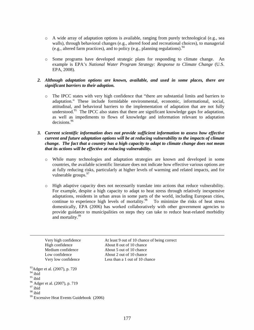
177

o A wide array of adaptation options is available, ranging from purely technological (e.g., sea

walls), through behavioral changes (e.g., altered food and recreational choices), to managerial (e.g., altered farm practices), and to policy (e.g., planning regulations).94

o Some programs have developed strategic plans for responding to climate change. An

example is EPA’s National Water Program Strategy: Response to Climate Change (U.S. EPA, 2008).

2. Although adaptation options are known, available, and used in some places, there are

significant barriers to their adoption.

o The IPCC states with very high confidence that “there are substantial limits and barriers to adaptation.” These include formidable environmental, economic, informational, social, attitudinal, and behavioral barriers to the implementation of adaptation that are not fully understood.95 The IPCC also states that there are significant knowledge gaps for adaptation, as well as impediments to flows of knowledge and information relevant to adaptation decisions.96

3. Current scientific information does not provide sufficient information to assess how effective

current and future adaptation options will be at reducing vulnerability to the impacts of climate change. The fact that a country has a high capacity to adapt to climate change does not mean that its actions will be effective at reducing vulnerability.

o While many technologies and adaptation strategies are known and developed in some

countries, the available scientific literature does not indicate how effective various options are at fully reducing risks, particularly at higher levels of warming and related impacts, and for vulnerable groups.97

o High adaptive capacity does not necessarily translate into actions that reduce vulnerability.

For example, despite a high capacity to adapt to heat stress through relatively inexpensive adaptations, residents in urban areas in some parts of the world, including European cities, continue to experience high levels of mortality.98 To minimize the risks of heat stress domestically, EPA (2006) has worked collaboratively with other government agencies to provide guidance to municipalities on steps they can take to reduce heat-related morbidity and mortality.99

Very high confidence At least 9 out of 10 chance of being correct High confidence About 8 out of 10 chance Medium confidence About 5 out of 10 chance Low confidence About 2 out of 10 chance Very low confidence Less than a 1 out of 10 chance

93Adger et al. (2007), p. 720 94 ibid 95 ibid 96 Adger et al. (2007), p. 719 97 ibid 98 ibid 99 Excessive Heat Events Guidebook (2006)

178

o Further research is needed to monitor progress on adaptation and to assess the direct as well as ancillary effects of adaptation measures.100

4. For any country–even one with high adaptive capacitySit is particularly difficult to reduce

vulnerability for all segments of the population. The most vulnerable and difficult to reach populations are the elderly, children, and the poor.

o The IPCC states with very high confidence that “adaptive capacity is uneven across and

within societies.” There are individuals and groups within all societies that have insufficient capacity to adapt to climate change.101

5. More adaptation will be required to reduce vulnerability to climate change. 102 Additional

adaptation can potentially reduce, but is never expected to completely eliminate, vulnerability to current and future climate change.

o According to the IPCC, “adaptation alone is not expected to cope with all the projected

effects of climate change, and especially not over the long term as most impacts increase in magnitude.” 103

6. A portfolio of adaptation and mitigation measures can diminish the risks associated with

climate change.

o Even the most stringent mitigation efforts cannot avoid further impacts of climate change in the next few decades, which makes adaptation essential, particularly in addressing near-term impacts. Unmitigated climate change would, in the long term, be likely to exceed the capacity of natural, managed, and human systems to adapt.104

100 Adger et al. (2007) p. 737 101 Adger et al. (2007), p. 719 102Adger et al. (2007), p. 719 103 IPCC (2007), p. 19 104 IPCC (2007), p. 20

179

References for Adaptation Appendix Adger, W.N., S. Agrawala, M.M.Q. Mirza, C. Conde, K. O’Brien, J. Pulhin, R. Pulwarty, B. Smit and K. Takahashi,

(2007) Assessment of adaptation practices, options, constraints and capacity. In: Climate Change 2007: Impacts, Adaptation and Vulnerability. Contribution of Working Group II to the Fourth Assessment Report of the Intergovernmental Panel on Climate Change [M.L. Parry, O.F. Canziani, J.P. Palutikof, P.J. van der Linden, and C.E. Hanson (eds.) Cambridge University Press, Cambridge, United Kingdom, pp. 717-743.

Excessive Heat Events Guidebook (2006). Report from the United States Environmental Protection Agency. 52

pages. June 2006. EPA 430-B-06-005. IPCC (2007) Summary for Policymakers. In: Climate Change 2007: Impacts, Adaptation and Vulnerability.

Contribution of Working Group II to the Fourth Assessment Report of the Intergovernmental Panel on Climate Change [M.L. Parry, O.F. Canziani, J.P. Palutikof, P.J. van der Linden and C.E. Hanson (eds.)]. Cambridge University Press, Cambridge, United Kingdom and New York, NY, USA.

U.S. EPA (2008) National Water Program Strategy: Response to Climate Change. Office of Water. EPA 800-R-

08001, September.

180

Appendix B: Greenhouse Gas Emissions From Section 202(a) Source Categories This Appendix provides greenhouse gas (GHG) emission information from Clean Air Act Section 202(a) source categories. It includes an overview of the respective source categories with a description of how the emission data from the Inventory of U.S. Greenhouse Gas Emissions and Sinks map to these source categories. Then, relevant emission data are presented and comparisons are made between U.S. GHG emissions from Section 202(a) source categories and domestic and global emission data. To inform the Administrator’s assessment, the following types of comparisons for both the collective and individual emissions of GHGs from Section 202(a) source categories are provided: As a share of total global aggregate emissions of the well-mixed GHGs As a share of total U.S. aggregate emissions of the six GHGs As a share of the total global transportation emissions of the six GHGs In addition, for each individual GHG, the following comparisons were also calculated: As a share of total U.S. Section 202(a) GHG emissions As a share of U.S. emissions of that individual GHG, including comparisons to the

magnitude of emissions of that GHG from non-transport related source categories As a share of global emissions of that individual GHG As a share of global transport GHG emissions As a share of all global GHG emissions (A) Overview of Section 202(a) Source Categories To inform the Administrator’s cause or contribute finding, EPA analyzed historical GHG emission data for motor vehicles and motor vehicle engines in the United States from 1990 to 2007 (the most recent year for which official EPA estimates are available). The motor vehicles and motor vehicle engines addressed include: Passenger cars Light-duty trucks Motorcycles Buses Medium/heavy-duty trucks The source of the emissions data is the Inventory of U.S. Greenhouse Gas Emissions and Sinks: 1990-2007 (U.S. EPA, 2009). The U.S. Inventory is organized around the source classification scheme put forth by the Intergovernmental Panel on Climate Change, in which emissions from motor vehicles and motor vehicle engines are reported within two different sectors: Energy and Industrial Processes. Table B.1 describes the correspondence between Section 202(a) GHG emission source categories and IPCC source categories:

181

Table B.1:Source Categories Included Under Section 202(a) Section 202(a) Source

Category IPCC Sector IPCC Source Category Greenhouse Gases Passenger Cars Energy 1A3b (i) Cars CO2, CH4, N2O Light-Duty Trucks Energy 1A3b (ii) Light-duty trucks CO2, CH4, N2O Motorcycles Energy 1A3b (iv) Motorcycles CO2, CH4, N2O Buses Energy 1A3b (iii) Heavy-duty trucks

and buses CO2, CH4, N2O

Medium/Heavy-Duty Trucks

Energy 1A3b (iii) Heavy-duty trucks and buses

CO2, CH4, N2O

Cooling (from section 202(a) sources)

Industrial Processes

2F1 Refrigeration and Air Conditioning Equipment

Hydrofluorocarbons (HFCs)

GHG emissions from aviation, pipelines, railways, and marine transport are included in the IPCC Energy Sector under 1A3 but are not included within Section 202(a). (B) GHG Emissions from Section 202(a) Source Categories (1) Total, combined GHG emissions from Section 202(a) source categories Table B.2 presents historical emissions of all GHGs (CO2, CH4, N2O, and HFCs) from Section 202(a) source categories from 1990-2007 in carbon dioxide equivalent units (TgCO2e).105 Passenger cars (38.7. percent), light-duty trucks (32.4 percent), and medium/heavy-duty trucks (24.8 percent) emitted the largest shares of GHG emissions in 2007, followed by cooling (from section 202(a) sources) (3.2 percent), buses (0.7 percent), and motorcycles (0.1 percent). From 1990 to 2007, GHG emissions from Section 202(a) source categories grew by 33.9 %due in part to increased demand for travel and the stagnation of fuel efficiency across the U.S. vehicle fleet. Since the 1970s, the number of highway vehicles registered in the United States has increased faster than the overall population, according to the Federal Highway Administration (FHWA).106 Likewise, the number of miles driven (up 41.3% from 1990 to 2007) and the gallons of gasoline consumed each year in the United States have increased steadily since the 1980s, according to the FHWA and Energy Information

105 A Tg is one teragram, or one million metric tons. 106 FHWA (1996 through 2008) Highway Statistics. Federal Highway Administration, U.S. Department of Transportation, Washington, DC. Report FHWA-PL-96-023-annual. Available online at <http://www.fhwa.dot.gov/policy/ohpi/hss/hsspubs.htm>.

182

Administration, respectively.107 These increases in motor vehicle use are the result of a confluence of factors, including population growth, economic growth, urban sprawl, low fuel prices, and increasing popularity of sport utility vehicles and other light-duty trucks that tend to have lower fuel efficiency.

107 DOE (1993 through 2008) Transportation Energy Data Book. Office of Transportation Technologies, Center for Transportation Analysis, Energy Division, Oak Ridge National Laboratory. ORNL-5198.

183

Table B.2: Total Greenhouse Gas Emissions by Section 202(a) Source Category (Tg CO2e) Section 202(a) Sources 1990 1995 2000 2001 2002 2003 2004 2005 2006 2007 Passenger Cars 656.9 633.9 670.3 673.1 686.5 664.4 660.7 677.3 651.1 639.6 Light-Duty Trucks 336.2 428.6 489.7 492.9 502.9 536.5 557.3 517.1 528.8 533.8 Motorcycles 1.8 1.8 1.9 1.7 1.7 1.7 1.8 1.7 1.9 2.1 Buses 8.3 9.0 10.9 10.0 9.7 10.5 14.7 11.8 12.1 12.1 Medium/Heavy-Duty Trucks 228.8 272.4 342.7 341.8 355.9 352.3 365.0 392.9 402.3 408.6 Cooling (from section 202(a) sources) 0.0 16.2 43.0 46.7 49.9 52.4 55.1 56.5 55.9 53.2 Total 1231.9 1362.1 1558.5 1566.3 1606.6 1617.7 1654.6 1657.3 1652.1 1649.3

Between 1990 and 2007, GHG emissions from passenger cars decreased 2.6%, though there was some growth in GHG emissions from 2000 to 2002, and again from 2004 to 2005. Emissions from light-duty trucks increased 58.8% from 1990 to2007, largely due to the increased use of sport-utility vehicles and other light-duty trucks. Meanwhile, GHG emissions from heavy-duty trucks increased 78.6%, reflecting the increased volume of total freight movement and an increasing share transported by trucks. In 1990, there were no hydrofluorocarbons (HFCs) used in vehicle cooling systems. HFCs were gradually introduced into motor vehicle air conditioning and refrigerating systems during the 1990s as chlorofluorocarbons (CFCs), and hydrochlorofluorocarbons (HCFCs) started to phase out of production as required under the Montreal Protocol and Title VI of the Clean Air Act. Table B.3 presents GHG emissions from Section 202(a) source categories alongside total U.S. emissions. The table also presents emissions from the electricity generation and industrial sectors for comparison. In 1990, Section 202(a) source categories emitted 20.2% of total U.S. emissions, behind the electricity generation sector (30.5%) and the industrial sector (24.5%). By 2007, Section 202(a) source categories collectively were the second largest sector with 23.1% of total U.S. emissions, due both to growth in vehicle emissions and a decline in emissions from industry.

184

Table B.3: Sectoral Comparison to Total U.S. Greenhouse Gas Emissions (Tg CO2e) U.S. Emissions 1990 1995 2000 2001 2002 2003 2004 2005 2006 2007 Section 202(a) GHG emissions 1231.9 1362.1 1558.5 1566.3 1606.6 1617.7 1654.6 1657.3 1652.1 1649.3

Share of U.S. (%) 20.2% 21.1% 22.2% 22.7% 23.1% 23.2% 23.4% 23.3% 23.4% 23.1% Electricity sector emissions 1859.1 1989.0 2329.3 2292.1 2301.1 2329.6 2362.0 2429.4 2375.5 2445.1

Share of U.S. (%) 30.5 30.8 33.2 33.2 33.1 33.4 33.4 34.2 33.7 34.2 Industrial sector emissions 1496.0 1524.5 1467.5 1415.0 1418.4 1394.7 1408.7 1364.9 1388.4 1386.3

Share of U.S. (%) 24.5 23.6 20.9 20.5 20.4 20.0 19.9 19.2 19.7 19.4 Total U.S. GHG emissions 6098.7 6463.3 7008.2 6896.3 6942.3 6981.1 7064.9 7108.6 7051.1 7150.1

Table B.4 compares total GHG emissions from Section 202(a) source categories to all U.S. GHG emissions, global GHG emissions from the transport sector (as defined by IPCC), and total global GHG emissions from all source categories, for 2005.108 Section 202(a) GHG emissions are a significantly larger share of global transport GHG emissions (28.0%) than the corresponding share of all U.S. GHG emissions to the global total (18.4%), reflecting the relative size of the transport sector in the United States compared to the global average. Section 202(a) GHG emissions were 4.3% of total global emissions in 2005. The global transport sector was 15.3% of all global emissions in 2005.

108 The year 2005 is the most recent year for which comprehensive greenhouse gas emissions data are available for all gases, all countries, and all sources. Global estimates are ‘gross’ emissions estimates and do not include removals of greenhouse gas emissions from the atmosphere by terrestrial sinks (i.e., forests and other biomass). Global data come from the World Resources Institute’s Climate Analysis Indicators Tool, which contains national data submitted by Parties to the UNFCCC, and other independent and peer-reviewed datasets (e.g., International Energy Agency).

185

Table B.4: Comparison to Global Greenhouse Gas Emissions (Tg CO2e)

2005 Sec 202(a) Share All U.S. GHG emissions 7,109 23.3% Global transport GHG emissions 5,925 28.0% All global GHG emissions 38,726 4.3%

(2) Individual GHG emissions from Section 202(a) source categories Table B.5 presents total GHG emissions from Section 202(a) source categories by gas, in CO2 equivalent units. In 2007, CO2 made up the largest share of emissions (95.1%), followed by HFCs (3.2%), N2O (1.6%) and CH4 (0.1%). Since 1990, the share of HFCs has increased (from zero in 1990), whereas the share of the other gases has correspondingly decreased. Methane and N2O emissions have decreased in absolute terms since 1990. Table B.5: Greenhouse Gas Emissions From Section 202(a) Source Categories by Gas (Tg CO2e)

Section 202(a) Sources 1990 1995 2000 2001 2002 2003 2004 2005 2006 2007 CO2 1187.3 1291.9 1463.8 1470.5 1512.0 1524.2 1561.4 1566.2 1564.9 1568.5

Share of Sec 202 GHGs 96% 95% 94% 94% 94% 94% 94% 95% 95% 95% CH4 4.2 3.8 2.9 2.8 2.4 2.2 2.1 1.9 1.8 1.7

Share of Sec 202 GHGs 0.34% 0.28% 0.18% 0.18% 0.15% 0.14% 0.13% 0.12% 0.11% 0.10% N2O 40.4 50.1 48.8 46.4 42.3 38.9 36.1 32.7 29.5 26.0

Share of Sec 202 GHGs 3.3% 3.7% 3.1% 3.0% 2.6% 2.4% 2.2% 2.0% 1.8% 1.6% HFCs 0.0 16.2 43.0 46.7 49.9 52.4 55.1 56.5 55.9 53.2

Share of Sec 202 GHGs 0.0% 1.2% 2.8% 3.0% 3.1% 3.2% 3.3% 3.4% 3.4% 3.2% Total GHGs 1231.9 1362.1 1558.5 1566.3 1606.6 1617.7 1654.6 1657.3 1652.1 1649.3

(a) Carbon dioxide emissions from Section 202(a) source categories Carbon dioxide is emitted from motor vehicles and motor vehicle engines during the fossil fuel combustion process. During combustion, the carbon (C) stored in the fuels is oxidized and emitted as CO2 and smaller amounts of other carbon compounds, including CH4, carbon monoxide (CO), and non-methane volatile organic compounds (NMVOCs). These other C-containing non-CO2 gases are emitted as by-products of incomplete fuel combustion, but are, for the most part, eventually oxidized to CO2 in the atmosphere.

186

As the dominant GHG emitted from motor vehicles and motor vehicle engines (95.1% of total emissions in 2007), CO2 emission trends in Table B.6 mirror those of the GHG emission total. Carbon dioxide emissions grew by 32.1% between 1990 and 2007. Most of this growth occurred as a result of increased CO2 emissions from light-duty trucks (62.8%) and medium/heavy-duty trucks (78.8%). Emissions from passenger cars did not grow over the same time period. Table B.6: CO2 Emissions by Section 202(a) Source Category (Tg CO2)

Sec. 202 Source Categories 1990 1995 2000 2001 2002 2003 2004 2005 2006 2007 Passenger Cars 628.8 604.9 643.5 647.9 662.6 642.1 640.0 658.4 634.4 625.0Light-Duty Trucks 320.7 405.0 466.2 470.5 483.5 519.1 541.2 502.8 515.5 522.0Motorcycles 1.7 1.8 1.8 1.7 1.7 1.6 1.7 1.6 1.9 2.0Buses 8.3 9.0 10.9 10.0 9.6 10.5 14.7 11.8 12.1 12.0Medium/Heavy-Duty Trucks 227.8 271.2 341.3 340.4 354.5 350.8 363.7 391.6 401.1 407.4Cooling (from section 202(a) sources) N/A N/A N/A N/A N/A N/A N/A N/A N/A N/A Total 1187.3 1291.9 1463.8 1470.5 1512.0 1524.2 1561.4 1566.2 1564.9 1568.5

Table B.7 presents CO2 emissions from Section 202(a) source categories alongside total U.S. CO2 emissions. The table also presents emissions from the electricity generation and industrial sectors for comparison. In 1990, Section 202(a) source categories emitted 23.4% of total U.S. CO2 emissions, behind the electricity generation sector (36.0%), and ahead of the industrial sector (22.3%). By 2007, emissions from Section 202(a) source categories increased to 25.7% of total U.S. CO2 emissions. Table B.7: Sectoral Comparison to Total U.S. CO2 Emissions (Tg CO2)

U.S. CO2 Emissions 1990 1995 2000 2001 2002 2003 2004 2005 2006 2007 Section 202 CO2 emissions 1187.3 1291.9 1463.8 1470.5 1512.0 1524.2 1561.4 1566.2 1564.9 1568.5

Share of U.S. CO2 (%) 23.4% 23.9% 24.6% 25.1% 25.6% 25.6% 25.8% 25.7% 26.0% 25.7%

Electricity Sector CO2 1829.7 1964.2 2311.7 2274.6 2284.0 2313.6 2345.0 2412.0 2358.3 2429.4

Share of U.S. CO2 (%) 36.0 36.3 38.8 38.8 38.7 38.8 38.8 39.6 39.2 39.8

Industrial Sector CO2 1132.6 1176.5 1148.6 1119.7 1122.5 1111.6 1130.4 1100.3 1126.0 1115.7

Share of U.S. CO2 (%) 22.3 21.8 19.3 19.1 19.0 18.6 18.7 18.1 18.7 18.3

Total U.S. CO2 emissions 5076.7 5407.9 5955.2 5860.0 5908.2 5963.2 6048.1 6090.8 6014.9 6103.4

187

Table B.8 compares total CO2 emissions from Section 202(a) source categories to total U.S. emissions, global GHG emissions from the transport sector (as defined by IPCC), and total global GHG emissions from all source categories, for 2005. Section 202(a) CO2 emissions are a significantly larger share of global transport GHG emissions (26.4%) than the corresponding share of all U.S. CO2 emissions to the global total (22.0%), reflecting the relative size of the transport sector in the U.S. compared to the global average. Section 202(a) CO2 emissions were 4.0% of total global GHG emissions in 2005. Table B.8: Comparison to U.S. and Global Greenhouse Gas Emissions (Tg CO2e)

Global Emissions 2005 Sec 202(a) CO2 Share

All U.S. GHG emissions 7,109 22.0%

All global CO2 emissions 27,526 5.7% Global transport GHG emissions 5,925 26.4% All global GHG emissions 38,726 4.0%

(b) Methane emissions from Section 202(a) source categories Methane emissions from motor vehicles are a function of the CH4 and hydrocarbon content of the motor fuel, the amount of hydrocarbons passing uncombusted through the engine, and any post-combustion control of hydrocarbon emissions (such as catalytic converters). Table B.9 shows the trend in CH4 emissions from Section 202(a) source categories since 1990, presented in carbon dioxide equivalents. The combustion of gasoline in passenger cars and light-duty trucks was responsible for the majority (91.2%) of the CH4 emitted from Section 202(a) source categories. From 1990 to 2007, CH4 emissions decreased by 61%. Table B.9: CH4 Emissions by Section 202(a) Source Category (Tg CO2e)

202(a) Sources 1990 1995 2000 2001 2002 2003 2004 2005 2006 2007 Passenger Cars 2.6 2.1 1.6 1.5 1.4 1.3 1.2 1.1 1.0 0.9 Light-Duty Trucks 1.4 1.4 1.1 1.1 0.9 0.8 0.7 0.7 0.7 0.6 Motorcycles 0.0 0.0 0.0 0.0 0.0 0.0 0.0 0.0 0.0 0.0 Buses 0.0 0.0 0.0 0.0 0.0 0.0 0.0 0.0 0.0 0.0 Medium/Heavy-Duty Trucks 0.2 0.2 0.1 0.1 0.1 0.1 0.1 0.1 0.1 0.1 Cooling (from section 202(a) sources) N/A N/A N/A N/A N/A N/A N/A N/A N/A` N/A Total 4.2 3.8 2.9 2.8 2.4 2.2 2.1 1.9 1.8 1.7

188

Table B.10 presents CH4 emissions from Section 202(a) source categories alongside total U.S. CH4 emissions. The table also presents CH4 emissions from landfills and natural gas systems for comparison. In 2007, Section 202(a) source categories emitted 0.3% of total U.S. CH4 emissions; landfills (22.7%) and natural gas systems (17.9.%) represented a significantly larger share. Overall, total U.S. CH4 emissions decreased by 5.1% (31.3 TgCO2e) from 1990 to 2007, in part due to efforts to reduce emissions at individual sources such as landfills and coal mines. Table B.10: Sectoral Comparison to Total U.S. CH4 Emissions (Tg CO2e)

U.S. CH4 Emissions 1990 1995 2000 2001 2002 2003 2004 2005 2006 2007 Section 202(a) CH4 emissions 4.2 3.8 2.9 2.8 2.4 2.2 2.1 1.9 1.8 1.7

Share of U.S. CH4 (%) 0.69 0.62 0.48 0.48 0.42 0.39 0.37 0.34 0.31 0.28 Landfill CH4 emissions 149.2 144.3 122.3 119.5 121.9 128.3 126.2 127.8 130.4 132.9

Share of U.S. CH4 (%) 24.2 23.4 20.7 20.7 21.0 22.2 22.4 22.8 22.4 22.7 Natural Gas CH4 emissions 129.6 132.6 130.8 129.5 129.0 127.2 118.0 106.3 104.8 104.7

Share of U.S. CH4 (%) 21.0 21.5 22.1 22.4 22.2 22.0 21.0 18.9 18.0 17.9

Total U.S. CH4 emissions 616.6 615.8 591.1 577.1 580.9 578.7 562.7 561.7 582.0 585.3 Table B.11 compares total CH4 emissions from Section 202(a) source categories to U.S. GHG emissions, global GHG emissions from the transport sector (as defined by IPCC), and total global GHG emissions from all source categories, for 2005. Section 202(a) CH4 emissions are a significantly smaller share of U.S., global transport, and global emissions in comparison to Section 202(a) CO2 emissions.

189

Table B.11: Comparison to US and global greenhouse gas emissions (Tg CO2e)

Global Emissions 2005 Sec 202(a) CH4 Share All U.S. GHG emissions 7,109 0.03% All global CH4 emissions 6,408 0.03% Global transport GHG emissions 5,925 0.03% All global GHG emissions 38,726 0.005%

(c) Nitrous oxide emissions from Section 202(a) source categories Nitrous oxide (N2O) is a product of the reaction that occurs between nitrogen and oxygen during fuel combustion. N2O emissions from motor vehicles and motor vehicle engines are closely related to fuel characteristics, air-fuel mixes, combustion temperatures, and the use of pollution control equipment. For example, some types of catalytic converters installed to reduce motor vehicle NOX, CO, and hydrocarbon emissions can promote the formation of N2O. Table B.12 shows the trend in N2O emissions from Section 202(a) source categories since 1990, presented in carbon dioxide equivalents. Section 202(a) emissions of N2O decreased by 35.55% from 1990 to 2007. Earlier generation control technologies initially resulted in higher N2O emissions, causing a 24.2% increase in N2O emissions from motor vehicles between 1990 and 1995. Improvements in later-generation emission control technologies have reduced N2O output, resulting in a 48.1% decrease in N2O emissions from 1995 to 2007. Overall, Section 202(a) N2O emissions were predominantly from gasoline-fueled passenger cars (52.8 %) and light-duty trucks (42.8%) in 2007. Table B.12: N2O Emissions by Section 202(a) Source Category (Tg CO2e)

202(a) Sources 1990 1995 2000 2001 2002 2003 2004 2005 2006 2007 Passenger Cars 25.4 26.9 25.2 23.8 22.5 21.0 19.5 17.8 15.7 13.7 Light-Duty Trucks 14.1 22.1 22.4 21.3 18.5 16.6 15.3 13.7 12.6 11.1 Motorcycles 0.0 0.0 0.0 0.0 0.0 0.0 0.0 0.0 0.0 0.0 Buses 0.0 0.0 0.0 0.0 0.0 0.0 0.0 0.0 0.0 0.0 Medium/Heavy-Duty Trucks 0.8 1.0 1.2 1.2 1.3 1.3 1.2 1.2 1.1 1.1 Cooling (from section 202(a) sources) N/A N/A N/A N/A N/A N/A N/A N/A N/A N/A Total 40.4 50.1 48.8 46.4 42.3 38.9 36.1 32.7 29.5 26.0

190

Table B.13 presents N2O emissions from Section 202(a) source categories alongside total U.S. N2O emissions. The table also presents N2O emissions from agricultural soil management and nitric acid production for comparison. In 2007, Section 202(a) source categories emitted 8.3% of total United States N2O emissions, making it the second largest source category. By far the largest source category in the United States is agricultural soil management, representing 66.7% of total N2O emissions in 2007. The third largest source in 2007 was nitric acid production (7.0%). Table B.13: Sectoral Comparison to Total U.S. N2O Emissions (Tg CO2e)

U.S. N2O Emissions 1990 1995 2000 2001 2002 2003 2004 2005 2006 2007 Section 202(a) N2O emissions 40.4 50.1 48.8 46.4 42.3 38.9 36.1 32.7 29.5 26.0

Share of U.S. N2O (%) 12.8 15.0 14.8 13.8 13.1 12.5 11.4 10.3 9.4 8.3 Agricultural Soil N2O emissions 200.3 202.3 204.5 220.4 207.6 202.8 211.2 210.6 208.4 207.9

Share of U.S. N2O (%) 63.6 60.6 62.1 65.5 64.5 64.9 66.4 66.7 66.8 66.7 Nitric Acid N2O emissions 20.0 22.3 21.9 17.8 19.3 18.1 18.0 18.6 18.2 21.7

Share of U.S. N2O (%) 6.3 6.7 6.7 5.3 6.0 5.8 5.6 5.9 5.8 7.0

Total U.S. N2O emissions 315.0 334.1 329.2 336.5 322.0 312.5 317.8 315.9 312.1 311.9

191

Table B.14 compares total N2O emissions from Section 202(a) source categories to U.S. GHG emissions, global GHG emissions from the transport sector (as defined by IPCC), total global N2O emissions, and total global GHG emissions from all source categories, for 2005. Section 202(a) N2O emissions are just under 0.55% of global transport emissions and 0.08% of all global GHG emissions. Table B.14: Comparison to U.S. and Global Greenhouse Gas Emissions (Tg CO2e)

2005 Sec 202(a) N2O Share All U.S. GHG emissions 7,109 0.46% All global N2O emissions 3,286 0.99% Global transport GHG emissions 5,925 0.55% All global GHG emissions 38,726 0.08%

(d) HFC emissions from Section 202(a) source categories HFCs (a term that encompasses a group of 11 related compounds) are progressively replacing CFCs and HCFCs in Section 202(a) cooling and refrigeration systems as they are being phased out under the Montreal Protocol and Title VI of the Clean Air Act.109 For example, HFC-134a has become a replacement for CFC-12 in mobile air conditioning systems. A number of HFC blends, containing multiple compounds, have also been introduced. The emission pathway can be complex, with HFCs being emitted to the atmosphere during the charging, operation, and decommissioning/disposal of cooling and refrigeration system. Table B.15 shows the trend in HFC emissions from Section 202(a) source categories since 1990, presented in carbon dioxide equivalents. As opposed to the GHGs discussed above, estimates of HFC emissions are presented here as the sum of HFC emissions from all vehicle modes that qualify as section 202(a) source categories. This was done because the U.S. Inventory does not disaggregate HFC emission data into vehicle types in exactly the same way as it does for other GHGs. The vehicle modes that are included in the HFC emission estimates are passenger cars, light-duty trucks and buses. Additionally, while HFC emissions associated with comfort cooling for passengers in medium and heavy duty trucks are considered a section 202(a) source, these emissions are not included here because they are not estimated for the U.S. Inventory due to insufficient data. As such, the numbers presented here are likely a slight underestimate of total section 202(a) HFC emissions. HFCs were not used in motor vehicles in 1990, but by 2007 emissions had increased to 53.2 Tg CO2e. From 1995 to 2007, HFC emissions from Section 202(a) source categories increased by 227%.

109 2006 IPCC Guidelines, Volume 3, Chapter 7. Page 43 (IPCC, 2006a).

192

Table B.15: HFC Emissions by Section 202(a) Source Category (Tg CO2e)

202(a) HFC Sources 1990 1995 2000 2001 2002 2003 2004 2005 2006 2007 Cooling (from section 202(a) sources) 0.0 16.2 43.0 46.7 49.9 52.4 55.1 56.5 55.9 53.2

Table B.16 presents HFC emissions from Section 202(a) source categories alongside total U.S. HFC emissions. The table also presents HFC emissions from HCFC-22 production and all other end-use applications of substitutes for ozone-depleting substances (ODS substitutes) for comparison. In 2007, Section 202(a) source categories emitted 42.4% of total U.S. HFC emissions, making it the largest source category. Other applications of ODS substitutes (including foam blowing, fire protection, aerosol propellants, solvents, and other applications) accounted for 44.1%. HCFC-22 chemical production results in byproduct releases of HFC-23, which accounted for 98.6% of HFC emissions in 1990, but declined by 2007 and now represents 13.5%. Table B.16: Sectoral Comparison to Total U.S. HFC Emissions (Tg CO2e)

U.S. HFC Emissions 1990 1995 2000 2001 2002 2003 2004 2005 2006 2007 Section 202(a) HFC emissions 0.0 16.2 43.0 46.7 49.9 52.4 55.1 56.5 55.9 53.2

Share of U.S. HFC (%) 0 26 43 48 48 52 49 49 46.9 42.4 HCFC-22 Production 36.4 33.0 28.6 19.7 21.1 12.3 17.2 15.8 13.8 17.0

Share of U.S. HFC (%) 98.6 53.4 28.6 20.4 20.2 12.1 15.3 13.6 11.6 13.5 Other ODS Substitutes 0.5 12.6 28.5 30.4 33.3 36.7 40.1 43.8 49.4 55.4

Share of U.S. HFC (%) 1.4 20.4 28.5 31.4 31.9 36.2 35.7 37.7 41.5 44.1 Total U.S. HFC emissions 36.9 61.8 100.1 96.9 104.3 101.4 112.4 116.1 119.1 125.5

Table B.17 compares total HFC emissions from Section 202(a) source categories to U.S. GHG emissions, global GHG emissions from the transport sector (as defined by IPCC), total global HFC emissions, and total global GHG emissions from all source categories, for 2005. Section 202(a) HFC emissions are 0.95% of global transport emissions and 0.15% of all global GHG emissions, but actually make up 14.8% of global HFC emissions. Table B.17: Comparison to U.S. and Global Greenhouse Gas Emissions (Tg CO2e)

2005 Sec 202(a) HFC Share All U.S. GHG emissions 7,109 0.79% All global HFC emissions 381 14.8% Global transport GHG emissions 5,925 0.95% All global GHG emissions 38,726 0.15%

193

(e) PFC and SF6 emissions Perfluorocarbons (PFCs) are not emitted from motor vehicles or motor vehicle engines in the United States. The main sources of PFC emissions in the United States are aluminum smelting and semiconductor manufacturing. Similarly, sulfur hexafluoride (SF6) is not emitted from motor vehicles or motor vehicle engines in the United States, although use of SF6 for tire inflation has been reported in other countries.110 The main sources of SF6 emissions in the United States are electrical transmission and distribution systems and primary magnesium smelting.

110 2006 IPCC Guidelines, Volume 3, Chapter 8 (IPCC, 2006b).

194

References for Appendix B DOE (1993 through 2008) Transportation Energy Data Book. Office of Transportation Technologies, Center for

Transportation Analysis, Energy Division, Oak Ridge National Laboratory. ORNL-5198. FHWA (1996 through 2008) Highway Statistics. Federal Highway Administration, U.S. Department of

Transportation, Washington, DC. Report FHWA-PL-96-023-annual. Available online at http://www.fhwa.dot.gov/policy/ohpi/hss/hsspubs.htm.

IPCC (2006a) Emissions of Fluorinated Substitues for Ozone Depleting Substances (Chapter 7), Industrial Processes

(Volume 3) In: 2006 IPCC Guidelines for National Greenhouse Gas Inventories, Prepared by the National Greenhouse Gas Inventories Programme, Eggleston H.S., Buendia L., Miwa K., Ngara T. and Tanabe K. (eds). Published: IGES, Japan.

IPCC (2006b) Other Product Manufacture and Use (Chapter 8), Industrial Processes (Volume 3) In: 2006 IPCC

Guidelines for National Greenhouse Gas Inventories, Prepared by the National Greenhouse Gas Inventories Programme, Eggleston H.S., Buendia L., Miwa K., Ngara T. and Tanabe K. (eds). Published: IGES, Japan.

U.S. EPA (2009) Inventory of U.S. Greenhouse Gas Emissions and Sinks: 1990 – 2007. EPA-430-R-09-004-004,

Washington, DC. WRI (2009) Climate Analysis Indicators Tool (CAIT) Version 6.0. Available at http://cait.wri.org/. Accessed

August 5, 2009.

195

Appendix C: Direct Effects of Ambient GHG Concentrations on Human Health Greenhouse gases (GHG), at both current and projected atmospheric concentrations, are not expected to pose exposure risks on human respiratory systems (i.e., breathing/inhalation). The literature supporting this conclusion is described below. Carbon dioxide (CO2) The direct effects of high CO2 concentrations on human health were assessed in the EPA (2000a) report, Carbon Dioxide as a Fire Suppressant: Examining the Risks, and have also been reviewed by the IPCC (2005) Special Report on Carbon Dioxide Capture and Storage. At concentrations above about 2%, CO2 has a strong effect on respiratory physiology, and at concentrations above 7 to 10%, it can cause unconsciousness and death (IPCC, 2005). Exposure studies have not revealed any adverse health effect of chronic exposure to concentrations below 1%. At concentrations greater than 17%, loss of controlled and purposeful activity, unconsciousness, convulsions, coma, and death occur within one minute of initial inhalation of CO2 (OSHA, 1989; CCOHS, 1990; Dalgaard et al., 1972; CATAMA, 1953; Lambertsen, 1971). But CO2 is a physiologically active gas and is a normal component of blood gases (U.S. EPA, 2000b). Acute CO2 exposure of up to 1% and 1.5% by volume is tolerated quite comfortably (U.S. EPA, 2000b). The ambient concentration of CO2 in the atmosphere is presently about 0.039% by volume (or 386 ppm). Projected increases in CO2 concentrations from anthropogenic emissions range from 41 to 158% above 2005 levels (of about 380 ppm) or 535 to 983 ppm by 2100 (Meehl et al., 2007) (see Section 5). Such increases would result in atmospheric CO2 concentrations of 0.054 to 0.098% by volume in 2100, which is well below published thresholds for adverse health effects. Methane (CH4) CH4 is flammable or explosive at concentrations of 5 to 15% by volume (50,000 to 150,000 ppm) of air (NIOSH, 1994; NRC, 2000). At high enough concentrations, CH4 is also a simple asphyxiant, capable of displacing enough oxygen to cause death by suffocation. Threshold limit values are not specified because the limiting factor is the available oxygen (NRC, 2000). Atmospheres with oxygen concentrations below 19.5% can have adverse physiological effects, and atmospheres with less than 16% oxygen can become life threatening (MSHA, 2007). Methane displaces oxygen to 18% in air when present at 14% (140,000 ppm). When oxygen is readily available, CH4 has little toxic effect (NRC, 2000). In assessing emergency exposure limits for CH4, the NRC (2000) determined that an exposure limit that presents an explosion hazard cannot be recommended, even if it is well below a concentration that would produce toxicity. As such, it recommended an exposure limit of 5,000 ppm for methane (NRC, 2000). The National Institute for Occupational Health Safety (NIOSH, 1994) established a threshold limit value (TLV) for methane at 1,000 ppm. The current atmospheric concentration of CH4 is 1.78 ppm. The projected CH4 concentration in 2100 ranges from 1.46 to 3.39 ppm by 2100, well below any recommended exposure limits (Meehl et al., 2007).

196

Nitrous Oxide (N2O)

N2O is an asphyxiant at high concentrations. At lower concentrations, exposure causes central nervous system, cardiovascular, hepatic (pertaining to the liver), hematopoietic (pertaining to the formation of blood or blood cells), and reproductive effects in humans (Hathaway et al., 1991). At a concentration of 50 to 67% (500,000 to 670,000 ppm) N2O is used to induce anesthesia in humans (Rom, 1992). NIOSH has established a recommended exposure limit (REL) for N2O of 25 ppm as a time-weighted average (TWA) for the duration of the exposure (NIOSH, 1992). The American Conference of Governmental Industrial Hygienists (ACGIH) has assigned N2O a TLV of 50 ppm as a TWA for a normal 8-hour workday and a 40-hour workweek (ACGIH, 1994). The NIOSH limit is based on the risk of reproductive system effects and decreases in audiovisual performance (NIOSH, 1992). The ACGIH limit is based on the risk of reproductive, hematological (related to the study of the nature, function, and diseases of the blood and of blood-forming organs), and nervous system effects (ACGIH, 1994). The current atmospheric concentration of N2O is 0.32 ppm. The projected N2O concentration in 2100 ranges from 0.36 to 0.46 ppm,, well below any exposure limits (Meehl et al., 2007). Fluorinated Gases (HFCs, PFCs, SF6) Most fluorinated gases emitted from anthropogenic activities are released in very small quantities relative to established thresholds for adverse health outcomes from exposure. The health effects of exposure to one illustrative HFC gas, one illustrative HCFC gas, and sulfur hexafluoride (SF6) are given in the context of their current atmospheric concentration. Chlorofluorocarbons are not included in this discussion given their phaseout under the Montreal Protocol. The NRC (1996) recommended a 1-hour emergency exposure guidance level (EEGL) of 4,000 ppm for HFC-134a. This recommendation was based on a no-observed-adverse-effect level of 40,000 ppm in cardiac-sensitization tests of male beagles (NRC, 1996). It recommended 24-hour EEGL of 1,000 ppm based on the fetotoxicity effects (slight retardation of skeletal ossification) observed in rats exposed to HFC-134a. Finally, it recommended a 90-day Continuous Exposure Guidance Level (CEGL) of 900 ppm based on a two-year chronic toxicity study conducted in male rats exposed to HFC-134a at different concentrations for six hours/day, five days/week. The atmospheric concentration of HFC 134a in 2003 was in the range of 26 to 31 parts per trillion according to IPCC/TEAP (2005), many orders of magnitude below EEGLs. For HCFC-123, the end points of pharmacological or adverse effects considered for establishing an EEGL are cardiac sensitization, anesthesia or CNS-related effects, malignant hyperthermia, and hepatotoxicity. According to the NRC (1996), the concentration required to produce cardiac sensitization in 50% of the animals for HCFC-123 was determined in dog studies to be 1.9% (19,000 ppm) for a 5-minute exposure. The NRC recommended that 1,900 ppm (19,000 ppm divided by an uncertainty factor of 10 for interspecies variability) should be considered the human no-observed-effect level for a 1-minute exposure to HCFC-123 on the basis of the dog cardiac-sensitization model. The concentration of HCFC-123 in 1996 was 0.03 parts per trillion according to IPCC/TEAP (2005), many orders of magnitude below the established effect level. SF6 is a relatively nontoxic gas but an asphyxiant at high concentrations. The NIOSH) recommended exposure limit is 1,000 ppm (NIOSH, 1997). The SF6 concentration in 2003 was about 5 parts per trillion according to IPCC/TEAP (2005), many orders of magnitude below the exposure limit.

197

References for Appendix C

ACGIH (1994) 1994-1995 Threshold limit values for chemical substances and physical agents and biological exposure indices. Cincinnati, OH: American Conference of Governmental Industrial Hygienists.

CATAMA (1953) Aviation Toxicology -- an Introduction to the Subject and a Handbook of Data. Committee on Aviation Toxicology, Aero Medical Association. The Blakiston Co.: New York, NY. pp. 6S9, 31S39, 52S55, 74S79, 110S115.

CCOHS (Canadian Centre for Occupational Health and Safety). 1990. CHEMINFO database search. Dalgaard, J.B., G. Dencker, B. Fallentin, P. Hansen, B. Kaempe, J. Steensberger, Wilhardt, P. (1972) Fatal

poisoning and other health hazards connected with industrial fishing. Br. J. Ind. Med. 29: 307S316. Hathaway GJ, NH Proctor, JP Hughes, and ML Fischman (1991) Proctor and Hughes' chemical hazards of the

workplace. 3rd ed. New York, NY: Van Nostrand Reinhold. IPCC (2005) Special Report on Carbon Dioxide Capture and Storage. A Special Report of Working Group III of the

Intergovernmental Panel on Climate Change. IPCC Technology and Economic Assessment Panel (2005) IPCC/TEAP Special Report on Safe-guarding the Ozone

Layer and the Global Climate System: Issues Related to Hydrofluorocarbons and Perfluorocarbons. Prepared by Working Group I and III of the IPCC, and the TEAP [B. Metz, L. Kuijpers, S. Solomon, S.O. Andersen, O. Davidson, J. Pons, D. de Jager, T. Kestin, M. Manning, and L.A. Meyers (eds.), Cambridge University Press, Cambridge, United Kingdom, and New York, NY, USA, 488 pp.

Lambertsen, C.J. (1971) “Therapeutic Gases—Oxygen, Carbon Dioxide, and Helium.” Drill’s Pharmacology in

Medicine. Chapter 556, [J.R. DiPalma (ed)], McGraw-Hill Book Co.: New York, NY. Meehl, G.A. et al. (2007) Global Climate Projections. In: Climate Change 2007: The Physical Science Basis.

Contribution of Working Group I to the Fourth Assessment Report of the Intergovernmental Panel on Climate Change [Solomon, S., D. Qin, M. Manning, Z. Chen, M. Marquis, K.B. Averyt, M. Tignor, and H.L. Miller (eds.)]. Cambridge University Press, Cambridge, United Kingdom and New York, NY, USA.

Mine Safety and Health Administration (MSHA) (2007) The Danger of Oxygen Deficiency in Underground Coal Mines. Department of Labor Program Information Bulletin NO. P07-05. http://www.msha.gov/regs/complian/PIB/2007/pib07-05.asp.

NIOSH (1997) NIOSH Pocket Guide to Chemical Hazards. U.S. Department of Health and Human Services, Public

Health Service, Centers for Disease Control and Prevention, Washington, D.C. NIOSH Publication no. 97-140; NTIS no. PB-97177604. http://www.cdc.gov/niosh/npg/npgd0576.html.

NIOSH (1994) International Chemical Safety CardsSMethane. U.S. Department of Health and Human Services,

Public Health Service, Centers for Disease Control and Prevention, Washington, D.C. http://www.cdc.gov/niosh/ipcsneng/neng0291.html.

NIOSH (1992) Recommendations for occupational safety and health: Compendium of policy documents and

statements. Cincinnati, OH: U.S. Department of Health and Human Services, Public Health Service, Centers for Disease Control, National Institute for Occupational Safety and Health (NIOSH) Publication No. 92-100.

National Research Council (NRC) (2000) Emergency and Continuous Exposure Limits for Selected Airborne

Contaminants, Volume 1. National Academy Press, Washington, D.C.

198

National Research Council (NRC) (1996) Toxicity of Alternatives to Chlorofluorocarbons: HFC-134a and HCFC-123. National Academy Press, Washington, D.C.

OSHA (1989) Carbon Dioxide, Industrial Exposure and Control Technologies for OSHA Regulated Hazardous

Substances, Volume I of II, Substance A - I. Occupational Safety and Health Administration. Washington, DC: U.S. Department of Labor. March.

Rom, WN (1992) Environmental and occupational medicine. 2nd ed. Boston, MA: Little, Brown and Company. U.S. EPA (2000a) Carbon Dioxide as a Fire Suppressant: Examining the Risks, EPA 430-R-00-002, May. U.S. EPA (2000b) Carbon Dioxide as a Fire Suppressant: Examining the Risks, Appendix B – Overview of Acute

Health Effects, EPA 430-R-00-002, May.