sequence textbook sequences and series
DESCRIPTION
Sequence Textbook Sequences and SeriesTRANSCRIPT

MOOCULUSmassive open online calculus
sequencesandseries
T H I S D O C U M E N T W A S T Y P E S E T O N A P R I L 1 7 , 2 0 1 4 .
Copyright © 2014 Jim Fowler and Bart Snapp
This work is licensed under the Creative Commons Attribution-NonCommercial-ShareAlike License. To view a copy of this license,visit http://creativecommons.org/licenses/by-nc-sa/3.0/ or send a letter to Creative Commons, 543 Howard Street,5th Floor, San Francisco, California, 94105, USA. If you distribute this work or a derivative, include the history of the document.
The source code is available at: https://github.com/kisonecat/sequences-and-series/tree/master/textbook
This text is based on David Guichard’s open-source calculus text which in turn is a modification and expansion of notes written byNeal Koblitz at the University of Washington. David Guichard’s text is available at http://www.whitman.edu/mathematics/calculus/ under a Creative Commons license.
The book includes some exercises and examples from Elementary Calculus: An Approach Using Infinitesimals, by H. Jerome Keisler,available at http://www.math.wisc.edu/~keisler/calc.html under a Creative Commons license. In addition, the chapteron differential equations and the section on numerical integration are largely derived from the corresponding portions of Keisler’sbook. Albert Schueller, Barry Balof, and Mike Wills have contributed additional material. Thanks to Walter Nugent, Nicholas J. Roux,Dan Dimmitt, Donald Wayne Fincher, Nathalie Dalpé, chas, Clark Archer, Sarah Smith, MithrandirAgain, AlmeCap, and hrzhu forproofreading and contributing on GitHub.
This book is typeset in the Kerkis font, Kerkis © Department of Mathematics, University of the Aegean.
We will be glad to receive corrections and suggestions for improvement at [email protected] or [email protected].
Contents
1 Sequences 13
1.1 Notation 13
1.2 Defining sequences 15
1.2.1 Defining sequences by giving a rule 15
1.2.2 Defining sequences using previous terms 16
1.3 Examples 17
1.3.1 Arithmetic sequences 18
1.3.2 Geometric sequences 18
1.3.3 Triangular numbers 19
1.3.4 Fibonacci numbers 20
1.3.5 Collatz sequence 21
1.4 Where is a sequence headed? Take a limit! 22
1.5 Graphs 24
1.6 New sequences from old 25
1.7 Helpful theorems about limits 27
1.7.1 Squeeze Theorem 28
1.7.2 Examples 29
4
1.8 Qualitative features of sequences 32
1.8.1 Monotonicity 33
1.8.2 Boundedness 34
2 Series 39
2.1 Definition of convergence 39
2.2 Geometric series 41
2.3 Properties of series 44
2.3.1 Constant multiple 44
2.3.2 Sum of series 47
2.4 Telescoping series 50
2.5 A test for divergence 51
2.6 Harmonic series 54
2.6.1 The limit of the terms 54
2.6.2 Numerical evidence 54
2.6.3 An analytic argument 55
2.7 Comparison test 56
2.7.1 Statement of the Comparison Test 56
2.7.2 Applications of the Comparison Test 57
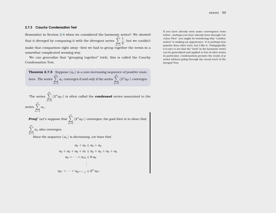
2.7.3 Cauchy Condensation Test 59
2.7.4 Examples of condensation 61
2.7.5 Convergence of p-series 63
5
3 Convergence tests 67
3.1 Ratio tests 67
3.1.1 Theory 68
3.1.2 Practice 71
3.2 Integral test 74
3.2.1 An example 74
3.2.2 Harmonic series 75
3.2.3 Statement of integral test 76
3.2.4 p-series 76
3.2.5 Integrating for approximations 78
3.3 More comparisons 81
3.4 The mostly useless root test 85
4 Alternating series 89
4.1 Absolute convergence 89
4.2 Alternating series test 93
5 Another comparison test 97
5.1 Convergence depends on the tail 98
5.2 Limit comparison test 101
5.2.1 Proof of the Limit Comparison Test 101
5.2.2 How to apply the Limit Comparison Test 102
6
6 Power series 105
6.1 Definitions 105
6.2 Convergence of power series 106
6.3 Power series centered elsewhere 110
6.4 Calculus with power series 114
7 Taylor series 117
7.1 Finding Taylor series 117
7.2 Taylor’s Theorem 126
Answers to Exercises 141
Index 147
How to read do mathematics
Reading mathematics is not the same as reading a novel—it’s more fun, and moreinteractive! To read mathematics you need
(a) a pen,
(b) plenty of blank paper, and
(c) the courage to write down everything—even “obvious” things.
As you read a math book, you work along with me, the author, trying to anticipatemy next thoughts, repeating many of the same calculations I did to write this book.You must write down each expression, sketch each graph, and constantly think
about what you are doing. You should work examples. You should fill-in the detailsI left out. This is not an easy task; it is hard work, but, work that is, I very muchhope, rewarding in the end.
Mathematics is not a passive endeavor. I may call you a “reader” but you arenot reading; you are writing this book for yourself.
—the so-called “author”


Acknowledgments
This text is a modification of David Guichard’s open-source calculus text which wasitself a modification of notes written by Neal Koblitz at the University of Washingtonand includes exercises and examples from Elementary Calculus: An Approach Using
Infinitesimals by H. Jerome Keisler. I am grateful to David Guichard for choosinga Creative Commons license. Albert Schueller, Barry Balof, and Mike Wills havecontributed additional material. The stylesheet, based on tufte-latex, wasdesigned by Bart Snapp.
This textbook was specifically used for a Coursera course called “Calculus Two:Sequences and Series.” Many thanks go to Walter Nugent, Donald Wayne Fincher,Robert Pohl, chas, Clark Archer, Mikhail, Sarah Smith, Mavaddat Javid, GrigoriyMikhalkin, Susan Stewart, Donald Eugene Parker, Francisco Alonso Sarría, EduardPascual Saez, Lam Tin-Long, mrBB, Demetrios Biskinis, Hanna Szabelska, RolandThiers, Sandra Peterson, Arthur Dent, Ryan Noble, Elias Sid, Faraz Rashid, andhrzhu for finding and correcting errors in early editions of this text. Thank you!
—Jim Fowler

Introduction, or. . . what is this all about?
Consider the following sum:
12+
14+
18+
116
+ · · ·+12i
+ · · ·
The dots at the end indicate that the sum goes on forever. Does this make sense?Can we assign a numerical value to an infinite sum? While at first it may seemdifficult or impossible, we have certainly done something similar when we talkedabout one quantity getting “closer and closer” to a fixed quantity. Here we couldask whether, as we add more and more terms, the sum gets closer and closer tosome fixed value. That is, look at
12=
12
34=
12+
14
78=
12+
14+
18
1516
=12+
14+
18+
116
and so on, and ask whether these values have a limit. They do; the limit is 1. Infact, as we will see,
12+
14+
18+
116
+ · · ·+12i
=2i − 1
2i= 1 −
12i
and thenlimi→∞
1 −12i
= 1 − 0 = 1.
12 sequences and series
This is less ridiculous than it appears at first. In fact, you might already believethat
0.33333̄ =310
+3
100+
31000
+3
10000+ · · · =
13
,
which is similar to the sum above, except with powers of ten instead of powers of two.And this sort of thinking is needed to make sense of numbers like π, considering
3.14159 . . . = 3 +110
+4
100+
11000
+5
10000+
9100000
+ · · · = π.
Before we investigate infinite sums—usually called series—we will investigatelimits of sequences of numbers. That is, we officially call
∞∑i=1
12i
=12+
14+
18+
116
+ · · ·+12i
+ · · ·
a series, while12
,34
,78
,1516
, . . . ,2i − 1
2i, . . .
is a sequence. The value of a series is the limit of a particular sequence, that is,
∞∑i=1
12i
= limi→∞
2i − 12i
.
If this all seems too obvious, let me assure you that there are twists and turnsaplenty. And if this all seems too complicated, let me assure you that we’ll be goingover this in much greater detail in the coming weeks. In either case, I hope thatyou’ll join us on our journey.
1 Sequences
1.1 Notation
Maybe you are feeling that this formality is unnec-essary, or even ridiculous; why can’t we just list offa few terms and pick up on the pattern intuitively?As we’ll see later, that might be very hard—nay,impossible—to do! There might be very different—but equally reasonable—patterns that start the sameway.
To resolve this ambiguity, it is perhaps not soridiculous to introduce the formalism of “functions.”Functions provide a nice language for associatingnumbers (terms) to other numbers (indices).
A “sequence” of numbers is just a list of numbers. For example, here is a list ofnumbers:
1, 1, 2, 3, 5, 8, 13, 21, . . .
Note that numbers in the list can repeat. And consider those little dots at theend! The dots “. . . ” signify that the list keeps going, and going, and going—forever.Presumably the sequence continues by following the pattern that the first few “terms”suggest. But what’s that pattern?
To make this talk of “patterns” less ambiguous, it is useful to think of a sequenceas a function. We have up until now dealt with functions whose domains are thereal numbers, or a subset of the real numbers, like f (x) = sin(1/x).
A real-valued function with domain the natural numbers N = {1, 2, 3, . . .} is asequence.
Other functions will also be regarded as sequences: the domain might include0 alongside the positive integers, meaning that the domain is the non-negativeintegers, Z≥0 = {0, 1, 2, 3, . . .}. The range of the function is still allowed to be thereal numbers; in symbols, the function f : N→ R is a sequence.
Sequences are written down in a few different, but equivalent, ways; you might
14 sequences and series
see a sequence written as
a1, a2, a3, . . . ,
an
(an)n∈N ,
{an}∞n=1 ,{
f (n)}∞n=1 , or
(f (n))n∈N ,
depending on which author you read. Worse, depending on the situation, thesame author (and this author) might use various notations for a sequence! In thistextbook, I will usually write (an) if I want to speak of the sequence as a whole(think gestalt) and I will write an if I am speaking of a specific term in the sequence.
Let’s summarize the preceding discussion in the following definition.
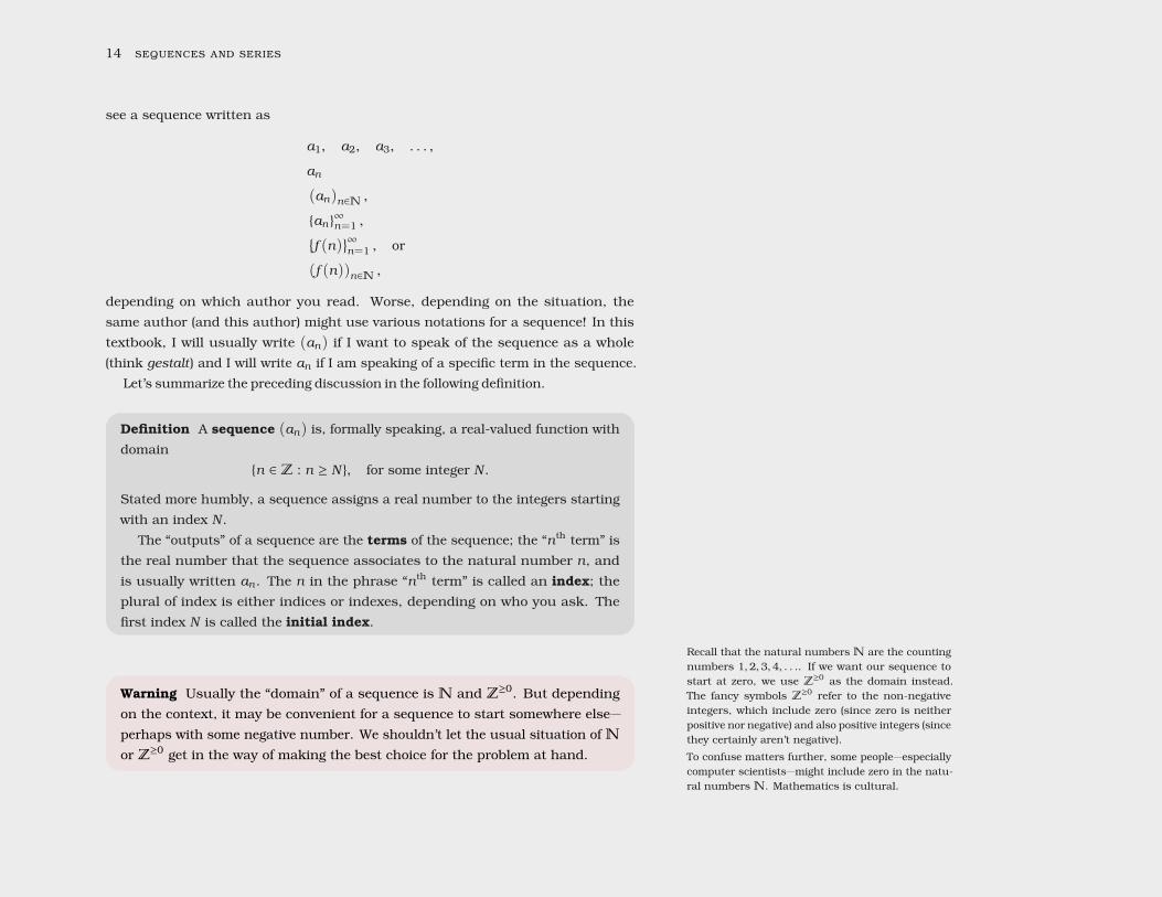
Definition A sequence (an) is, formally speaking, a real-valued function withdomain
{n ∈ Z : n ≥ N}, for some integer N .
Stated more humbly, a sequence assigns a real number to the integers startingwith an index N .
The “outputs” of a sequence are the terms of the sequence; the “nth term” isthe real number that the sequence associates to the natural number n, andis usually written an. The n in the phrase “nth term” is called an index; theplural of index is either indices or indexes, depending on who you ask. Thefirst index N is called the initial index.
Recall that the natural numbers N are the countingnumbers 1, 2, 3, 4, . . .. If we want our sequence tostart at zero, we use Z≥0 as the domain instead.The fancy symbols Z≥0 refer to the non-negativeintegers, which include zero (since zero is neitherpositive nor negative) and also positive integers (sincethey certainly aren’t negative).To confuse matters further, some people—especiallycomputer scientists—might include zero in the natu-ral numbers N. Mathematics is cultural.
Warning Usually the “domain” of a sequence is N and Z≥0. But dependingon the context, it may be convenient for a sequence to start somewhere else—perhaps with some negative number. We shouldn’t let the usual situation of N
or Z≥0 get in the way of making the best choice for the problem at hand.
sequences 15
As you can tell, there is a deep tension between precise definition and a vagueflexibility; as instructors, how we navigate that tension will be a big part of whetherwe are successful in teaching the course. We need to invoke precision when we’retempted to be too vague, and we need to reach for an extra helping of vaguenesswhen the formalism is getting in the way of our understanding. It can be a toughbalance.
1.2 Defining sequences
1.2.1 Defining sequences by giving a rule
Just as real-valued functions from Calculus One were usually expressed by aformula, we will most often encounter sequences that can be expressed by aformula. In the Introduction to this textbook, we saw the sequence given by the ruleai = f (i) = 1 − 1/2i . Other examples are easy to cook up, like
ai =i
i + 1,
bn =12n
,
cn = sin(nπ/6), or
di =(i − 1)(i + 2)
2i.
Frequently these formulas will make sense if thought of either as functions withdomain R or N, though occasionally the given formula will make sense only forintegers. We’ll address the idea of a real-valued function “filling in” the gaps betweenthe terms of a sequence when we look at graphs in Section 1.5.
Warning A common misconception is to confuse the sequence with the rulefor generating the sequence. The sequences (an) and (bn) given by the rulesan = (−1)n and bn = cos(π n) are, despite appearances, different rules whichgive rise to the same sequence. These are just different names for the same
16 sequences and series
object.
Let’s give a precise definition for “the same” when speaking of sequences. Compare this to equality for functions: two func-tions are the same if they have same domain andcodomain, and they assign the same value to eachpoint in the domain.Definition Suppose (an) and (bn) are sequences starting at 1. These se-
quences are equal if for all natural numbers n, we have an = bn.More generally, two sequences (an) and (bn) are equal if they have the same
initial index N , and for every integer n ≥ N , the nth terms have the same value,that is,
an = bn for all n ≥ N .
In other words, sequences are the same if they have the same set of valid indexes,and produce the same real numbers for each of those indexes—regardless of whetherthe given “rules” or procedures for computing those sequences resemble each otherin any way.
1.2.2 Defining sequences using previous termsYou might be familiar with recursion from a computerscience course.Another way to define a sequence is recursively, that is, by defining the later outputs
in terms of previous outputs. We start by defining the first few terms of the sequence,and then describe how later terms are computed in terms of previous terms.
Example 1.2.1 Define a sequence recursively by
a1 = 1, a2 = 3, a3 = 10,
and the rule that an = an−1 − an−3. Compute a5.
Solution First we compute a4. Substituting 4 for n in the rule an = an−1 −
an−3, we finda4 = a4−1 − a4−3 = a3 − a1.
But we have values for a3 and a1, namely 10 and 1, respectively. Thereforea4 = 10 − 1 = 9.
Now we are in a position to compute a5. Substituting 5 for n in the rule
sequences 17
an = an−1 − an−3, we find
a5 = a5−1 − a5−3 = a4 − a2.
We just computed a4 = 9; we were given a2 = 3. Therefore a5 = 9 − 3 = 6.
You can imagine some very complicated sequencesdefined recursively. Make up your own sequenceand share it with your friends! Use the hashtag#sequence.
1.3 Examples
Tons of entertaining sequences are listed in the TheOn-Line Encyclopedia of Integer Sequences.Mathematics proceeds, in part, by finding precise statements for everyday concepts.
We have already done this for sequences when we found a precise definition(“function from N to R”) for the everyday concept of “a list of real numbers.” Butall the formalisms in the world aren’t worth the paper they are printed on if therearen’t some interesting examples of those precise concepts. Indeed, mathematicsproceeds not only by generalizing and formalizing, but also by focusing on specific,concrete instances. So let me share some specific examples of sequences.
But before I can share these examples, let me address a question: how can Ihand you an example of a sequence? It is not enough just to list off the first fewterms. Let’s see why.
Example 1.3.1 Consider the sequence (an)
a1 = 41, a2 = 43, a3 = 47, a4 = 53, . . .
What is the next term a5? Can you identify the sequence?
This particular polynomial n2 −n+41 is rather inter-esting, since it outputs many prime numbers. Youcan read more about it at the OEIS.
Solution In spite of many so-called “intelligence tests” that ask questions justlike this, this question simply doesn’t have an answer. Or worse, it has toomany answers!
This sequence might be “the prime numbers in order, starting at 41.” Ifthat’s the case, then the next term is a5 = 59. But maybe this sequence is thesequence given by the polynomial an = n2 − n + 41. If that’s the case, thenthe next term is a5 = 61. Who is to say which is the “better” answer?
Recall that a prime number is an integer greaterthan one that has no positive divisors besides itselfand one.
Now let’s consider two popular “families” of sequences.
18 sequences and series
1.3.1 Arithmetic sequences
The first family1 we consider are the “arithmetic” sequences. Here is a definition. 1 Mathematically, the word family does not have anentirely precise definition; a family of things is acollection or a set of things, but family also has aconnotation of some sort of relatedness.Definition An arithmetic progression (sometimes called an arithmetic se-
quence) is a sequence where each term differs from the next by the same, fixedquantity.
Example 1.3.2 An example of an arithmetic progression is the sequence (an)
which begins
a1 = 10, a2 = 14, a3 = 18, a4 = 22, . . .
and which is given by the rule an = 6 + 4n. Each term differs from theprevious by four.
In general, an arithmetic progression in which subsequent terms differ by m canbe written as
an = m (n − 1) + a1.
Alternatively, we could describe an arithmetic progression recursively, by giving astarting value a1, and using the rule that an = an−1 +m. Why are arithmetic progressions called arithmetic?
Note that every term is the arithmetic mean, thatis, the average, of its two neighbors.
An arithmetic progression can decrease; for instance,
17, 15, 13, 11, 9, . . .
is an arithmetic progression.
1.3.2 Geometric sequences
The second family we consider are geometric progressions.
sequences 19
Definition A geometric progression (sometimes called a geometric sequence)is a sequence where the ratio between subsequent terms is the same, fixedquantity.
Example 1.3.3 An example of a geometric progression is the sequence (an)
startinga1 = 10, a2 = 30, a3 = 90, a4 = 270, . . .
and given by the rule an = 10 · 3n−1. Each term is three times the precedingterm.
In general, a geometric progression in which the ratio between subsequent termsis r can be written as
an = a1 · rn−1.
Alternatively, we could describe a geometric progression recursively, by giving astarting value a1, and using the rule that an = r · an−1. Why are geometric progressions called geometric?
Note that every term is the geometric mean of itstwo neighbors. The geometric mean of two numbersa and b is defined to be
√ab.
Of course, that raises another question: why isthe geometric mean called geometric? One geometricinterpretation of the geometric mean of a and b isthis: the geometric mean is the side length of asquare whose area is equal to that of the rectanglehaving side lengths a and b.
A geometric progression needn’t be increasing. For instance, in the followinggeometric progression
75
,710
,720
,740
,780
,7
160, . . .
the ratio between subsequent terms is one half, and each term is smaller than theprevious.
1.3.3 Triangular numbers
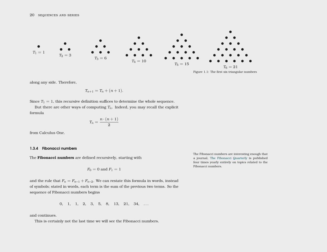
The sequence of triangular numbers (Tn) is a sequence of integers counting thenumber of dots in increasingly large “equilateral triangles” built from dots. The termTn is the number of dots in a triangle with n dots to a side.
There are a couple of ways of making this discussion more precise. Given anequilateral triangle with n dots to a side, how many more dots do you need to buildthe equilateral triangle with n + 1 dots to a side? All you need to do to transformthe smaller triangle to the larger triangle is an additional row of n + 1 dots placed
20 sequences and series
T1 = 1T2 = 3
T3 = 6T4 = 10
T5 = 15T6 = 21
Figure 1.1: The first six triangular numbers
along any side. Therefore,
Tn+1 = Tn + (n + 1).
Since T1 = 1, this recursive definition suffices to determine the whole sequence.But there are other ways of computing Tn. Indeed, you may recall the explicit
formula
Tn =n · (n + 1)
2
from Calculus One.
1.3.4 Fibonacci numbersThe Fibonacci numbers are interesting enough thata journal, The Fibonacci Quarterly is publishedfour times yearly entirely on topics related to theFibonacci numbers.
The Fibonacci numbers are defined recursively, starting with
F0 = 0 and F1 = 1
and the rule that Fn = Fn−1 + Fn−2. We can restate this formula in words, insteadof symbols; stated in words, each term is the sum of the previous two terms. So thesequence of Fibonacci numbers begins
0, 1, 1, 2, 3, 5, 8, 13, 21, 34, . . .
and continues.This is certainly not the last time we will see the Fibonacci numbers.
sequences 21
1.3.5 Collatz sequence
Here is a fun sequence with which to amuse your friends—or distract your enemies.Let’s start our sequence with a1 = 6. Subsequent terms are defined using the rule
an =
an−1/2 if an−1 is even, and
3an−1 + 1 if an−1 is odd.
Let’s compute a2. Since a1 is even, we follow the instructions in the first line, to findthat a2 = a1/2 = 3. To compute a3, note that a2 is odd so we follow the instructionin the second line, and a3 = 3a2 + 1 = 3 · 3 + 1 = 10. Since a3 is even, the firstline applies, and a4 = a3/2 = 10/2 = 5. But a4 is odd, so the second line applies,and we find a5 = 3 · 5+ 1 = 16. And a5 is even, so a6 = 16/2 = 8. And a6 is even,so a7 = 8/4 = 4. And a7 is even, so a8 = 4/2 = 2, and then a9 = 2/2 = 1. Oh,but a9 is odd, so a10 = 3 · 1 + 1 = 4. And it repeats. Let’s write down the start ofthis sequence:
6, 3, 10, 5, 16, 8, 4, 2, 1, 4, 2, 1,
repeats︷ ︸︸ ︷4, 2, 1, 4, . . .
What if we had started with a number other than six? What if we set a1 = 25 butthen we used the same rule? In that case, since a1 is odd, we compute a2 by finding3a1 + 1 = 3 · 25 + 1 = 76. Since 76 is even, the next term is half that, meaninga3 = 38. If we keep this up, we find that our sequence begins
25, 76, 38, 19, 58, 29, 88, 44, 22, 11, 34, 17, 52, 26,
13, 40, 20, 10, 5, 16, 8, 4, 2, 1, . . .
and then it repeats “4, 2, 1, 4, 2, 1, . . . ” just like before. If you think you have an argument that answersthe Collatz conjecture, I challenge you to try yourhand at the 5x + 1 conjecture, that is, use the rule
an =
an−1/2 if an−1 is even, and5an−1 + 1 if an−1 is odd.
Does this always happen? Is it true that no matter which positive integer youstart with, if you apply the half-if-even, 3x + 1-if-odd rule, you end up getting stuckin the “4, 2, 1, . . . ” loop? That this is true is the Collatz conjecture; it has beenverified for all starting values below 5× 260. Nobody has found a value which doesn’treturn to one, but for all anybody knows there might well be a very large initial valuewhich doesn’t return to one; nobody knows either way. It is an unsolved problem2 2 This is not the last unsolved problem we will en-
counter in this course. There are many things whichhumans do not understand.
in mathematics.
22 sequences and series
1.4 Where is a sequence headed? Take a limit!
We’ve seen a lot of sequences, and already there are a few things we might notice.For instance, the arithmetic progression
1, 8, 15, 22, 29, 36, 43, 50, 57, 64, 71, 78, 85, 92, . . .
just keeps getting bigger and bigger. No matter how large a number you think of, ifI add enough 7’s to 1, eventually I will surpass the giant number you thought of.On the other hand, the terms in a geometric progression where each term is halfthe previous term, namely
12
,14
,18
,116
,132
,164
,1
128,
1256
,1
512,
11024
, . . . ,
are getting closer and closer to zero. No matter how close you stand near but not atzero, eventually this geometric sequence gets even closer than you are to zero.
These two sequences have very different stories. One shoots off to infinity; theother zooms in towards zero. Mathematics is not just about numbers; mathematicsprovides tools for talking about the qualitative features of the numbers we dealwith. What about the two sequences we just considered? They are qualitatively verydifferent. The first “goes to” infinity; the second “goes to” zero. If you were with us in Calculus One, you are perhaps
already guessing that by “goes to,” I actually mean“has limit.”
In short, given a sequence, it is helpful to be able to say something qualitativeabout it; we may want to address the question such as “what happens after a while?”Formally, when faced with a sequence, we are interested in the limit
limi→∞
f (i) = limi→∞
ai .
In Calculus One, we studied a similar question about
limx→∞
f (x)
when x is a variable taking on real values; now, in Calculus Two, we simply want torestrict the “input” values to be integers. No significant difference is required in thedefinition of limit, except that we specify, perhaps implicitly, that the variable is aninteger.

sequences 23
Definition Suppose that (an) is a sequence. To say that limn→∞
an = L is to saythat
for every ε > 0,there is an N > 0,
so that whenever n > N ,we have |an − L | < ε.
If limn→∞
an = L we say that the sequence converges. If there is no finite value Lso that lim
n→∞an = L, then we say that the limit does not exist, or equivalently
that the sequence diverges.
The definition of limit is being written as if it werepoetry, what with line breaks and all. Like the bestof poems, it deserves to be memorized, performed,internalized. Humanity struggled for millenia to findthe wisdom contained therein.
Warning In the case that limn→∞
an = ∞, we say that (an) diverges, or perhaps
more precisely, we say (an) diverges to infinity. The only time we say that asequence converges is when the limit exists and is equal to a finite value.
One way to compute the limit of a sequence is to compute the limit of a function.
Theorem 1.4.1 Let f (x) be a real-valued function. If an = f (n) definesa sequence (an) and if lim
x→∞f (x) = L in the sense of Calculus One, then
limn→∞
an = L as well.
Example 1.4.2 Since limx→∞
(1/x) = 0, it is clear that also limn→∞
(1/n) = 0; inother words, the sequence of numbers
11
,12
,13
,14
,15
,16
, . . .
get closer and closer to 0, or more precisely, as close as you want to get to zero,after a while, all the terms in the sequence are that close.
More precisely, no matter what ε > 0 we pick, we can find an N big enoughso that, whenever n > N , we have that 1/n is within ε of the claimed limit,
24 sequences and series
zero. This can be made concrete: let’s suppose we set ε = 0.17. What is asuitable choice for N in response? If we choose N = 5, then whenever n > 5we have 0 < 1/n < 0.17.
But it is important to note that the converse3 of this theorem is not true. To 3 The converse of a statement is what you get whenyou swap the assumption and the conclusion; theconverse of “if it is raining, then it is cloudy” is thestatement “if it is cloudy, then it is raining.” Whichof those statements is true?
show the converse is not true, it is enough to provide a single example where it fails.Here’s the counterexample4.
4 An instance of (a potential) general rule being bro-ken is called a counterexample. This is a popularterm among mathematicians and philosophers.
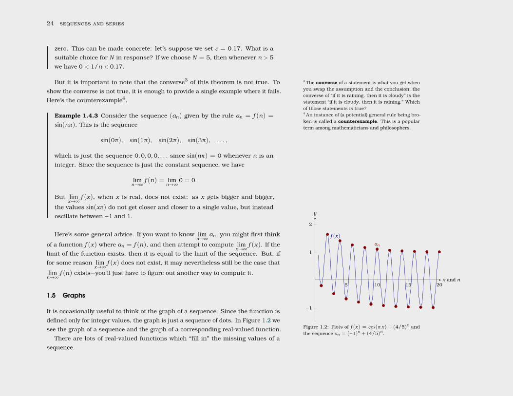
Example 1.4.3 Consider the sequence (an) given by the rule an = f (n) =
sin(nπ). This is the sequence
sin(0π), sin(1π), sin(2π), sin(3π), . . . ,
which is just the sequence 0, 0, 0, 0, . . . since sin(nπ) = 0 whenever n is aninteger. Since the sequence is just the constant sequence, we have
limn→∞
f (n) = limn→∞
0 = 0.
But limx→∞
f (x), when x is real, does not exist: as x gets bigger and bigger,
the values sin(xπ) do not get closer and closer to a single value, but insteadoscillate between −1 and 1.
Here’s some general advice. If you want to know limn→∞
an, you might first think
of a function f (x) where an = f (n), and then attempt to compute limx→∞
f (x). If thelimit of the function exists, then it is equal to the limit of the sequence. But, iffor some reason lim
x→∞f (x) does not exist, it may nevertheless still be the case that
limn→∞
f (n) exists—you’ll just have to figure out another way to compute it.
5 10 15 20
−1
1
2
f (x)
an
x and n
y
Figure 1.2: Plots of f (x) = cos(π x) + (4/5)x andthe sequence an = (−1)n + (4/5)n .
1.5 Graphs
It is occasionally useful to think of the graph of a sequence. Since the function isdefined only for integer values, the graph is just a sequence of dots. In Figure 1.2 wesee the graph of a sequence and the graph of a corresponding real-valued function.
There are lots of real-valued functions which “fill in” the missing values of asequence.
sequences 25
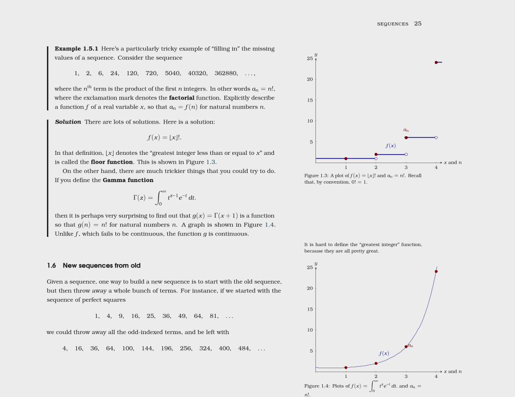
Example 1.5.1 Here’s a particularly tricky example of “filling in” the missingvalues of a sequence. Consider the sequence
1, 2, 6, 24, 120, 720, 5040, 40320, 362880, . . . ,
where the nth term is the product of the first n integers. In other words an = n!,where the exclamation mark denotes the factorial function. Explicitly describea function f of a real variable x, so that an = f (n) for natural numbers n.
1 2 3 4
5
10
15
20
25
f (x)
an
x and n
y
Figure 1.3: A plot of f (x) = bxc! and an = n!. Recallthat, by convention, 0! = 1.
Solution There are lots of solutions. Here is a solution:
f (x) = bxc!.
In that definition, bxc denotes the “greatest integer less than or equal to x” andis called the floor function. This is shown in Figure 1.3.
On the other hand, there are much trickier things that you could try to do.If you define the Gamma function
Γ(z) =∫ ∞
0tz−1e−t dt.
then it is perhaps very surprising to find out that g(x) = Γ(x + 1) is a functionso that g(n) = n! for natural numbers n. A graph is shown in Figure 1.4.Unlike f , which fails to be continuous, the function g is continuous.
It is hard to define the “greatest integer” function,because they are all pretty great.
1 2 3 4
5
10
15
20
25
f (x)
an
x and n
y
Figure 1.4: Plots of f (x) =∫ ∞
0tze−t dt. and an =
n!.
1.6 New sequences from old
Given a sequence, one way to build a new sequence is to start with the old sequence,but then throw away a whole bunch of terms. For instance, if we started with thesequence of perfect squares
1, 4, 9, 16, 25, 36, 49, 64, 81, . . .
we could throw away all the odd-indexed terms, and be left with
4, 16, 36, 64, 100, 144, 196, 256, 324, 400, 484, . . .

26 sequences and series
We say that this latter sequence is a subsequence of the original sequence. Here isa precise definition.
Definition Suppose (an) is a sequence with initial index N , and suppose wehave a sequence of integers (ni) so that
N ≤ n1 < n2 < n3 < n4 < n5 < · · ·
Then the sequence (bi) given by bi = ani is said to be a subsequence of thesequence an.
Limits are telling the story of “what happens” to a sequence. If the terms of asequence can be made as close as desired to a limiting value L, then the subsequencemust share that same fate.
Theorem 1.6.1 If (bi) is a subsequence of the convergent sequence (an), thenlimi→∞
bi = limn→∞
an.
Of course, just because a subsequence converges does not mean that the largersequence converges, too. We’ll see this again in more detail when we get toExample 1.7.6, but we’ll discuss it briefly now.
Example 1.6.2 Find a convergent subsequence of the sequence (an) given bythe rule an = (−1)n.
Solution Note that the sequence (an) does not converge. But by consideringthe sequence of indexes ni = 2 · i, we can build a subsequence
bi = ani = a2i = (−1)2i = 1,
which is a constant sequence, so it converges to 1.
sequences 27
There are other subsequences of an = (−1)n which converge but do not convergeto one. For instance, the subsequence of odd indexed terms is the constant sequencecn = −1, which converges to −1. For that matter, the fact that there are convergentsubsequences with distinct limits perhaps explains why the original sequence (an)
does not converge. Let’s formalize this.
Corollary 1.6.3
Suppose (bi) and (ci) are convergent subsequences of the sequence (an),but
limi→∞
bi , limi→∞
ci .
Then the sequence (an) does not converge.
Proof Suppose, on the contrary, the sequence (an) did converge. Then by
Theorem 1.6.1, the subsequence (bi) would converge, too, and
limi→∞
bi = limn→∞
an .
Again by Theorem 1.6.1, the subsequence (ci) would converge, too, and
limi→∞
ci = limn→∞
an .
But then limi→∞
bi = limi→∞
ci , which is exactly what we are supposing doesn’t
happen! To avoid this contradiction, it must be that our original assumption that
(an) converged was incorrect; in short, the sequence (an) does not converge.
1.7 Helpful theorems about limits
Not surprisingly, the properties of limits of real functions translate into propertiesof sequences quite easily.
28 sequences and series
Theorem 1.7.1 Suppose that limn→∞
an = L and limn→∞
bn = M and k is someconstant. Then
limn→∞
kan = k limn→∞
an = kL,
limn→∞
(an + bn) = limn→∞
an + limn→∞
bn = L +M ,
limn→∞
(an − bn) = limn→∞
an − limn→∞
bn = L −M ,
limn→∞
(anbn) = limn→∞
an · limn→∞
bn = LM , and
limn→∞
anbn
=limn→∞ anlimn→∞ bn
=L
M, provided M , 0.
1.7.1 Squeeze Theorem
Likewise, there is an analogue of the squeeze theorem for functions.
Theorem 1.7.2 Suppose there is some N so that for all n > N , it is the casethat an ≤ bn ≤ cn. If
limn→∞
an = limn→∞
cn = L
, then limn→∞
bn = L.
And a final useful fact:
Theorem 1.7.3 limn→∞
|an | = 0 if and only if limn→∞
an = 0.
Sometimes people write “iff” as shorthand for “if andonly if.”This says simply that the size of an gets close to zero if and only if an gets close
to zero.
sequences 29
1.7.2 Examples
Armed with these helpful theorems, we are now in a position to work a number ofexamples.
Example 1.7.4 Determine whether the sequence (an) given by the rule an =n
n + 1converges or diverges. If it converges, compute the limit.
Solution Consider the real-valued function
f (x) =x
x + 1.
Since an = f (n), it will be enough to find limx→∞
f (x) in order to find limn→∞
an . Wecompute, as in Calculus One, that
limx→∞
x
x + 1= lim
x→∞
(x + 1) − 1x + 1
= limx→∞
(x + 1x + 1
−1
x + 1
)= lim
x→∞
(1 −
1x + 1
)= lim
x→∞1 − lim
x→∞
1x + 1
= 1 − limx→∞
1x + 1
= 1 − 0 = 1.
We therefore conclude that limn→∞
an = 1.
And this is reasonable: by choosing n to be a largeenough integer, I can make
n
n + 1as close to 1 as I
would like. Just imagine how close1000000000010000000001is to one.
Example 1.7.5 Determine whether the sequence (an) given by an =lognn
converges or diverges. If it converges, compute the limit.
Solution By l’Hôpital’s rule, we compute
limx→∞
log xx
= limx→∞
1/x1
= 0.
30 sequences and series
Therefore,
limn→∞
lognn
= 0.
I’m not too fond of l’Hôpital’s rule, so I would havebeen happier if I had given a solution that didn’tinvolve it; you could avoid mentioning l’Hôpital’srule in Example 1.7.5 if you used, say, the squeezetheorem and the fact that logn ≤
√n.
Example 1.7.6 Determine whether the sequence (an) given by the rule an =
(−1)n converges or diverges. If it converges, compute the limit.
Solution Your first inclination might be to consider the “function” f (x) =
(−1)x , but you’ll run into trouble when trying to tell me the value of f (1/2).How does the sequence an = (−1)n begin? It starts
−1, 1, −1, 1, −1, 1, −1, 1, −1, 1, . . . ,
so the sequence isn’t getting close to any number in particular.Intuitively, the above argument is probably pretty convincing. But if you
want an airtight argument, you can reason like this: suppose—though we’llsoon see that this is a ridiculous assumption—that the sequence an = (−1)n
did converge to L. Then any subsequence would also converge to L, byTheorem 1.6.1 which stated that the limit of a subsequence is the same as thelimit of the original sequence. If I throw away every other term of the sequence(an), I am left with the constant sequence
−1, −1, −1, −1, −1, −1, −1, . . . ,
which converges to −1, and so L must be −1.On the other hand, if I throw away all the terms with odd indices and keep
only those terms with even indices, I am left with the constant subsequence
1, 1, 1, 1, 1, 1, 1, . . . ,
so L must be 1. Since L can’t be both −1 and 1, it couldn’t have been the casethat lim
n→∞an = L for a real number L. In other words, the limit does not exist.
I imagine that the “airtight argument” in the solutionto Example 1.7.6 is difficult to understand. Pleasedon’t worry if you find the argument confusing now—we’ll have more opportunities for doing these sortsof proofs by contradiction in the future.
sequences 31
Example 1.7.7 Determine whether the sequence an = (−1/2)n converges ordiverges. If it converges, compute the limit.
In this problem, you must be very careful to recognizethe difference between (−1/2)n and −(1/2)n . Theformer flip-flops between being positive and beingnegative, while the latter is always negative.
Solution Let’s use the Squeeze Theorem. Consider the sequences bn =
−(1/2)n and cn = (1/2)n. Then bn ≤ an ≤ cn. And limn→∞
cn = 0 because
limx→∞
(1/2)x = 0. Since bn = −cn, we have limn→∞
bn = − limn→∞
cn = −0 = 0.Since bn and cn converge to zero, the squeeze theorem tells us that lim
n→∞an = 0
as well.If you don’t want to mention the Squeeze Theorem, you could instead
apply Theorem 1.7.3. In that case, we would again consider the sequencecn = |an | and observe that lim
n→∞cn = 0. But then Theorem 1.7.3 steps in,
and tells us that limn→∞
an = 0 as well. Of course, a convincing argument forwhy Theorem 1.7.3 works at all goes via the squeeze theorem, so this secondmethod is not so different from the first.
Example 1.7.8 Determine whether an =sinn√n
converges or diverges. If it
converges, compute the limit.
Solution Since −1 ≤ sinn ≤ 1, we have
−1√n≤
sinn√n≤
1√n
,
and can therefore apply the Squeeze Theorem. Since limx→∞
1√x= 0, we get
limn→∞
−1√n= lim
n→∞
1√n= 0,
and so by squeezing, we conclude limn→∞
an = 0.
You might be wondering why I love the SqueezeTheorem so much; one reason is that the SqueezeTheorem gets you into the idea of “comparing” onesequence to another, and this “comparison” idea willbe big when we get to convergence tests in Chapter 3.
Example 1.7.9 A particularly common and useful sequence is the geometricprogression an = rn for a fixed real number r. For which values of r does thissequence converge?
32 sequences and series
Solution It very much does depend on r.If r = 1, then an = (1)n is the constant sequence
1, 1, 1, 1, 1, 1, 1, 1, . . . ,
so the sequence converges to one. A similarly boring fate befalls the case r = 0,in which case an = (0)n converges to zero.
If r = −1, we are reprising the sequence which starred in Example 1.7.6; aswe saw, that sequence diverges.
If either r > 1 or r < −1, then the terms an = rn can be made as large asone likes by choosing n large enough (and even), so the sequence diverges.
If 0 < r < 1, then the sequence converges to 0.If −1 < r < 0 then |rn | = |r |n and 0 < |r | < 1, so the sequence {|r |n}∞n=0
converges to 0, so also {rn}∞n=0 converges to 0.
That last example of a geometric progression is involved enough that it deservesto be summarized as a theorem.
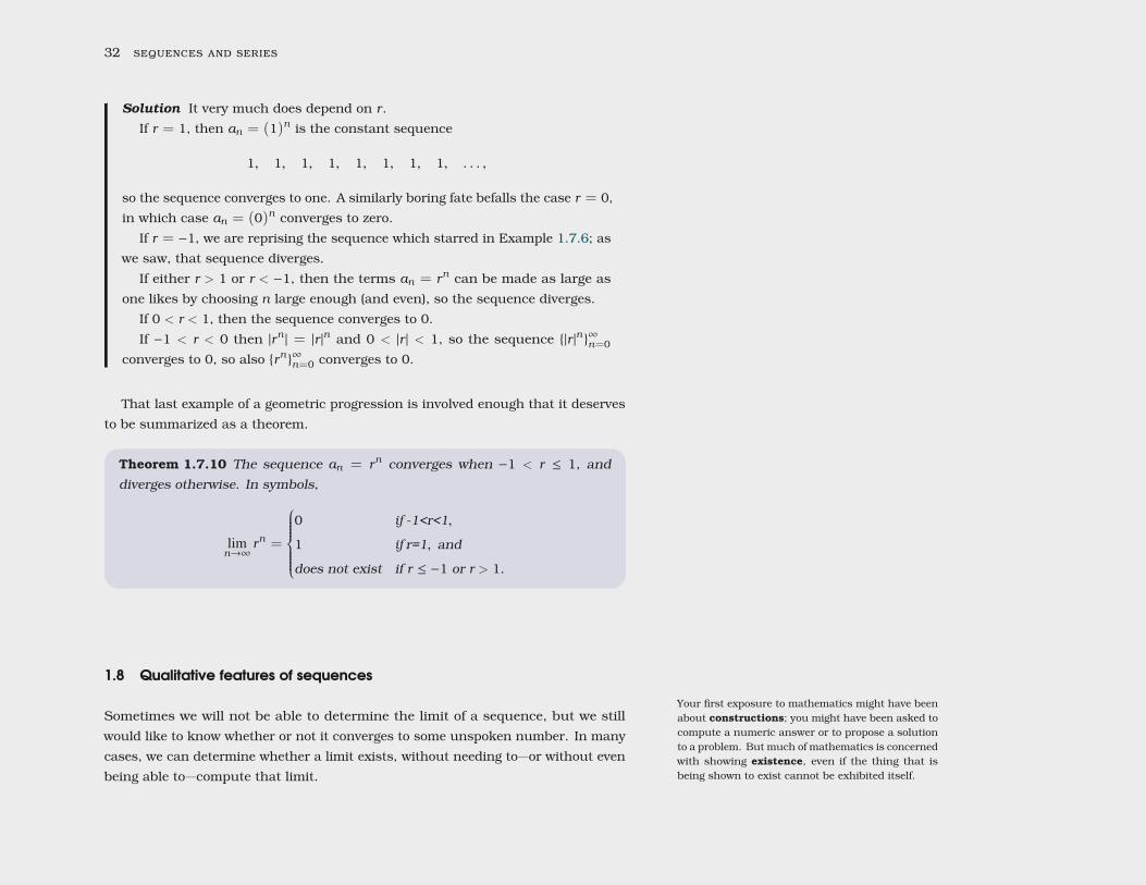
Theorem 1.7.10 The sequence an = rn converges when −1 < r ≤ 1, anddiverges otherwise. In symbols,
limn→∞
rn =
0 if -1<r<1,
1 if r=1, and
does not exist if r ≤ −1 or r > 1.
1.8 Qualitative features of sequences
Your first exposure to mathematics might have beenabout constructions; you might have been asked tocompute a numeric answer or to propose a solutionto a problem. But much of mathematics is concernedwith showing existence, even if the thing that isbeing shown to exist cannot be exhibited itself.
Sometimes we will not be able to determine the limit of a sequence, but we stillwould like to know whether or not it converges to some unspoken number. In manycases, we can determine whether a limit exists, without needing to—or without evenbeing able to—compute that limit.
sequences 33
1.8.1 Monotonicity
And sometimes we don’t even care about limits, but we’d simply like some terminol-ogy with which to describe features we might notice about sequences. Here is someof that terminology. For instance, how much money I have on day n is
a sequence; I probably hope that sequence is anincreasing sequence.
Definition A sequence is called increasing (or sometimes strictly increasing)if an < an+1 for all n. It is called non-decreasing if an ≤ an+1 for all n.
Similarly a sequence is decreasing (or, by some people, strictly decreasing)if an > an+1 for all n and non-increasing if an ≥ an+1 for all n.
To make matters worse, the people who insist on saying “strictly increasing” may—much to everybody’s confusion—insist on calling a non-decreasing sequence “in-creasing.” I’m not going to play their game; I’ll be careful to say “non-decreasing”when I mean a sequence which is getting larger or staying the same.
To make matters better, lots of facts are true for sequences which are eitherincreasing or decreasing; to talk about this situation without constantly saying“either increasing or decreasing,” we can make up a single word to cover both cases.
Definition If a sequence is increasing, non-decreasing, decreasing, or non-increasing, it is said to be monotonic.
Let’s see some examples of sequences which are monotonic.
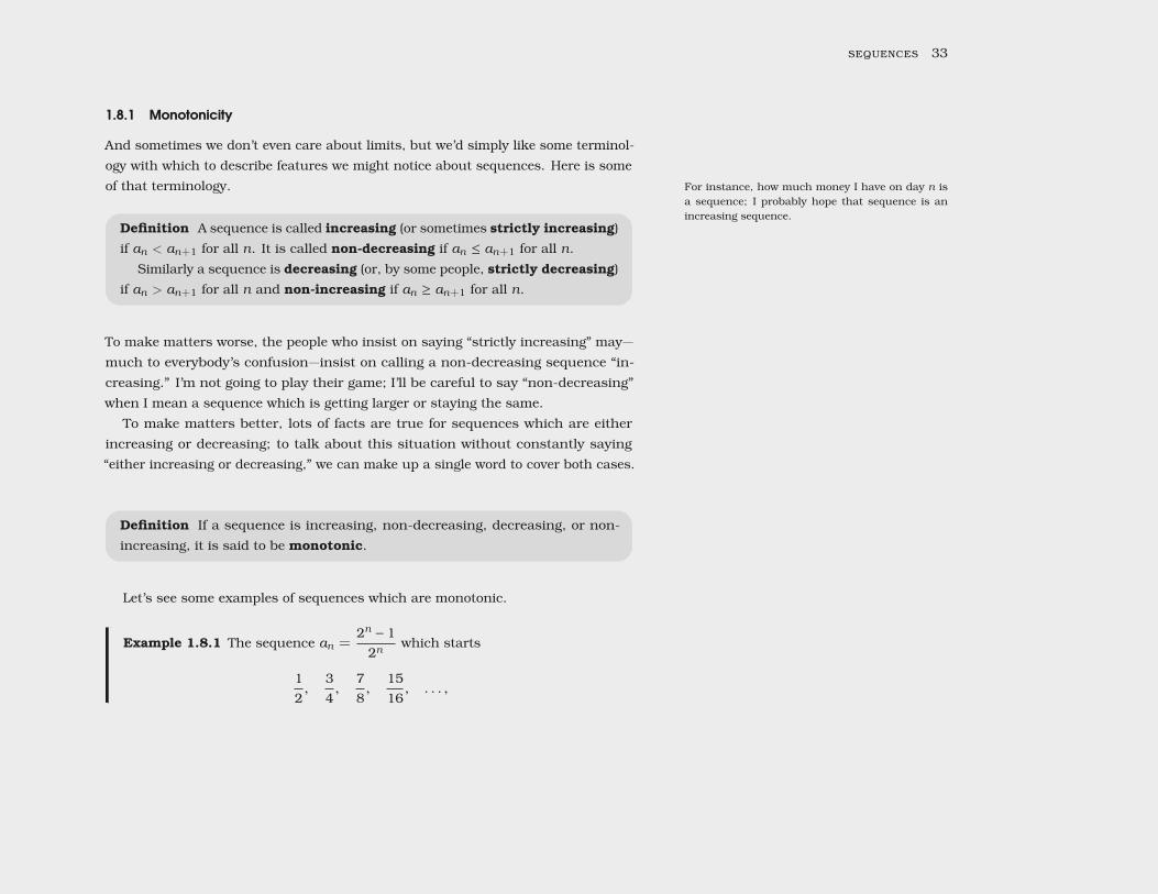
Example 1.8.1 The sequence an =2n − 1
2nwhich starts
12
,34
,78
,1516
, . . . ,
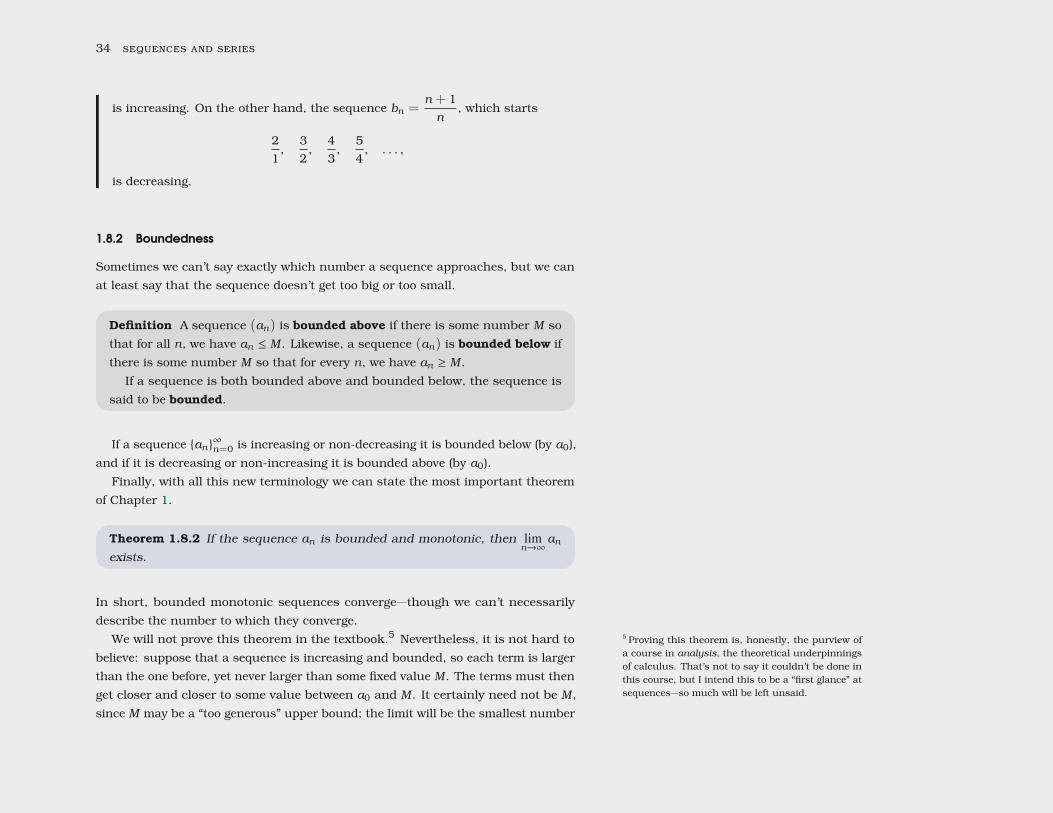
34 sequences and series
is increasing. On the other hand, the sequence bn =n + 1n
, which starts
21
,32
,43
,54
, . . . ,
is decreasing.
1.8.2 Boundedness
Sometimes we can’t say exactly which number a sequence approaches, but we canat least say that the sequence doesn’t get too big or too small.
Definition A sequence (an) is bounded above if there is some number M sothat for all n, we have an ≤ M . Likewise, a sequence (an) is bounded below ifthere is some number M so that for every n, we have an ≥ M .
If a sequence is both bounded above and bounded below, the sequence issaid to be bounded.
If a sequence {an}∞n=0 is increasing or non-decreasing it is bounded below (by a0),and if it is decreasing or non-increasing it is bounded above (by a0).
Finally, with all this new terminology we can state the most important theoremof Chapter 1.
Theorem 1.8.2 If the sequence an is bounded and monotonic, then limn→∞
anexists.
In short, bounded monotonic sequences converge—though we can’t necessarilydescribe the number to which they converge.
We will not prove this theorem in the textbook.5 Nevertheless, it is not hard to 5 Proving this theorem is, honestly, the purview ofa course in analysis, the theoretical underpinningsof calculus. That’s not to say it couldn’t be done inthis course, but I intend this to be a “first glance” atsequences—so much will be left unsaid.
believe: suppose that a sequence is increasing and bounded, so each term is largerthan the one before, yet never larger than some fixed value M . The terms must thenget closer and closer to some value between a0 and M. It certainly need not be M,since M may be a “too generous” upper bound; the limit will be the smallest number
sequences 35
that is above6 all of the terms an. Let’s try an example! 6 This concept of the “smallest number above all theterms” is an incredibly important one; it is the idea ofa least upper bound that underlies the real numbers.Example 1.8.3 All of the terms (2i − 1)/2i are less than 2, and the sequence
is increasing. As we have seen, the limit of the sequence is 1—1 is the smallestnumber that is bigger than all the terms in the sequence. Similarly, all ofthe terms (n + 1)/n are bigger than 1/2, and the limit is 1—1 is the largestnumber that is smaller than the terms of the sequence.
We don’t actually need to know that a sequence is monotonic to apply thistheorem—it is enough to know that the sequence is “eventually” monotonic,7 that is, 7 After all, the limit only depends on what is hap-
pening after some large index, so throwing away thebeginning of a sequence won’t affect its convergenceor its limit.
that at some point it becomes increasing or decreasing. For example, the sequence10, 9, 8, 15, 3, 21, 4, 3/4, 7/8, 15/16, 31/32, . . . is not increasing, because amongthe first few terms it is not. But starting with the term 3/4 it is increasing, so ifthe pattern continues and the sequence is bounded, the theorem tells us that the“tail” 3/4, 7/8, 15/16, 31/32, . . . converges. Since convergence depends only onwhat happens as n gets large, adding a few terms at the beginning can’t turn aconvergent sequence into a divergent one.
Example 1.8.4 Show that the sequence (an) given by an = n1/n converges.
You may be worried about my saying that log 3 > 1.If log were the common (base 10) logarithm, thiswould be wrong, but as far as I’m concerned, thereis only one log, the natural log. Since 3 > e, we mayconclude that log 3 > 1.
Solution We might first show that this sequence is decreasing, that is, weshow that for all n,
n1/n > (n + 1)1/(n+1).
36 sequences and series
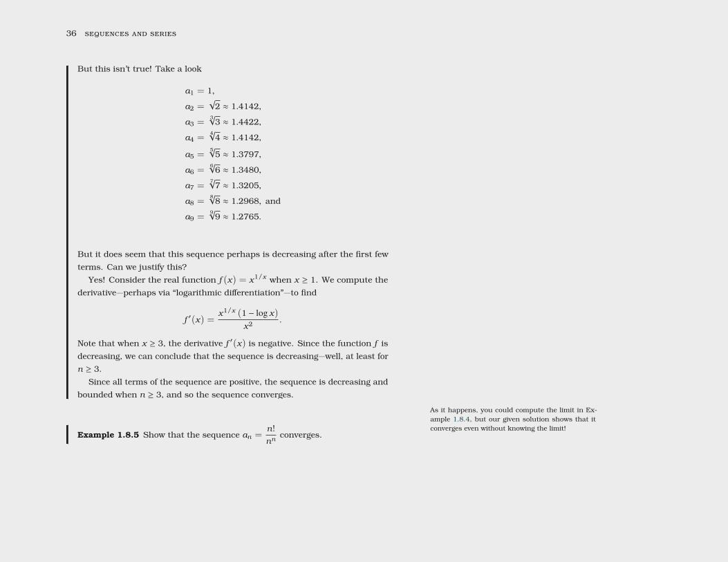
But this isn’t true! Take a look
a1 = 1,
a2 =√
2 ≈ 1.4142,
a3 =3√3 ≈ 1.4422,
a4 =4√4 ≈ 1.4142,
a5 =5√5 ≈ 1.3797,
a6 =6√6 ≈ 1.3480,
a7 =7√7 ≈ 1.3205,
a8 =8√8 ≈ 1.2968, and
a9 =9√9 ≈ 1.2765.
But it does seem that this sequence perhaps is decreasing after the first fewterms. Can we justify this?
Yes! Consider the real function f (x) = x1/x when x ≥ 1. We compute thederivative—perhaps via “logarithmic differentiation”—to find
f ′(x) =x1/x (1 − log x)
x2 .
Note that when x ≥ 3, the derivative f ′(x) is negative. Since the function f isdecreasing, we can conclude that the sequence is decreasing—well, at least forn ≥ 3.
Since all terms of the sequence are positive, the sequence is decreasing andbounded when n ≥ 3, and so the sequence converges.
As it happens, you could compute the limit in Ex-ample 1.8.4, but our given solution shows that itconverges even without knowing the limit!
Example 1.8.5 Show that the sequence an =n!nn
converges.
sequences 37
Solution Let’s get an idea of what is going on by computing the first few terms.
a1 = 1, a2 =12
, a3 =29≈ 0.22222, a4 =
332≈ 0.093750,
a5 =24625
≈ 0.038400, a6 =5
324≈ 0.015432,
a7 =720
117649≈ 0.0061199, a8 =
315131072
≈ 0.0024033.
The sequence appears to be decreasing. To formally show this, we would needto show an+1 < an, but we will instead show that
an+1
an< 1,
which amounts to the same thing. It is helpful trick here to think of the ratiobetween subsequent terms, since the factorials end up canceling nicely. Inparticular,
an+1
an=
(n + 1)!(n + 1)n+1
nn
n!
=(n + 1)!n!
nn
(n + 1)n+1
=n + 1n + 1
( n
n + 1
)n=
( n
n + 1
)n< 1.
Note that the sequence is bounded below, since every term is positive.Because the sequence is decreasing and bounded below, it converges.
Indeed, Exercise 2 asks you to compute the limit.
These sorts of arguments involving the ratio of subsequent terms will come upagain in a big way in Section 3.1. Stay tuned!
38 sequences and series
Exercises for Section 1.8
(1) Compute limx→∞
x1/x . à
(2) Use the squeeze theorem to show that limn→∞
n!nn
= 0. à
(3) Determine whether {√n + 47 −
√n}∞n=0 converges or diverges. If it converges, compute
the limit. à
(4) Determine whether{n2 + 1(n + 1)2
}∞n=0
converges or diverges. If it converges, compute the
limit. à
(5) Determine whether{
n + 47√n2 + 3n
}∞n=1
converges or diverges. If it converges, compute the
limit. à
(6) Determine whether{
2n
n!
}∞n=0
converges or diverges. If it converges, compute the limit.
à
2 Series
We’ve only just scratched the surface of sequences, and already we’ve arrived inChapter 2. Series will be the main focus of our attention for the rest of the course. Ifthat’s the case, then why did we bother with sequences? Because a series is what
you get when you add up the terms of a sequence, in order. So we needed totalk about sequences to provide the language with which to discuss series.
Suppose (an) is a sequence; then the associated series1 1 The Σ symbol may look like an E, but it is the Greekletter sigma, and it makes an S sound—just like thefirst letter of the word “series.” If you see “GRΣΣK,”say “grssk.”
∞∑k=1
ak = a1 + a2 + a3 + a4 + a5 + · · ·
I might be thinking that I feel just fine, but I have woken a terrible beast! Whatdoes that innocuous looking “· · · ” mean? What does it mean to add up infinitelymany numbers? It’s not as if I’ll ever be done with all the adding, so how can I everattach a “value” to a series? How can I do infinitely many things, yet live to sharethe answer with you?
I can’t.But I can do a large, but finite, number of things, and then see if I’m getting close
to anything in particular. In other words, I can take a limit.
2.1 Definition of convergence
But a limit. . . of what? From a sequence, we can consider the associated series, andassociated to that series is a yet another sequence—the sequence of partial sums.Here’s a formal definition which unwinds this tangled web.
40 sequences and series
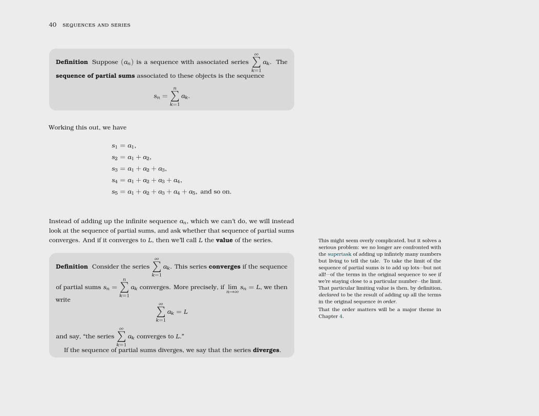
Definition Suppose (an) is a sequence with associated series∞∑k=1
ak . The
sequence of partial sums associated to these objects is the sequence
sn =n∑
k=1ak .
Working this out, we have
s1 = a1,
s2 = a1 + a2,
s3 = a1 + a2 + a3,
s4 = a1 + a2 + a3 + a4,
s5 = a1 + a2 + a3 + a4 + a5, and so on.
Instead of adding up the infinite sequence an, which we can’t do, we will insteadlook at the sequence of partial sums, and ask whether that sequence of partial sumsconverges. And if it converges to L, then we’ll call L the value of the series. This might seem overly complicated, but it solves a
serious problem: we no longer are confronted withthe supertask of adding up infintely many numbersbut living to tell the tale. To take the limit of thesequence of partial sums is to add up lots—but notall!—of the terms in the original sequence to see ifwe’re staying close to a particular number—the limit.That particular limiting value is then, by definition,declared to be the result of adding up all the termsin the original sequence in order.
That the order matters will be a major theme inChapter 4.
Definition Consider the series∞∑k=1
ak . This series converges if the sequence
of partial sums sn =n∑
k=1ak converges. More precisely, if lim
n→∞sn = L, we then
write∞∑k=1
ak = L
and say, “the series∞∑k=1
ak converges to L.”
If the sequence of partial sums diverges, we say that the series diverges.
series 41
Remember, infinity is not a number. So if it happens that limn→∞
n∑k=1
ak = ∞, then
we might write∞∑k=1
ak = ∞ but nevertheless we still say that the series diverges. Sometimes, to emphasize that the series involvesadding up infinitely many terms, we will say “infi-nite series” instead of just “series.”
2.2 Geometric series
Armed with the official definition of convergence in general, we focus in on the specificexample: a sequence of the form an = a0 r
n is called a geometric progression aswe learned back in Subsection 1.3.2. What happens when we add up the terms of ageometric progression? A geometric series was used by Archimedes—who
lived more than two thousand years ago!—to computethe area between a parabola and a straight line.Humans had the first inklings of calculus a very longtime ago.
Definition (Geometric Series) A series of the form
∞∑k=0
a0 rk
is called a geometric series.
We can’t simply “add” up the infinitely many terms in the geometric series. Whatwe can do, instead, is add up the a first handful of terms. Pick a big value for n,and instead compute
sn =n∑
k=0a0 r
k = a0 + a0 r + a0 r2 + a0 r
3 + · · ·+ a0 rn .
42 sequences and series
This is the nth partial sum. Concretely,
s0 = a0,
s1 = a0 + a0 r,
s2 = a0 + a0 r + a0 r2,
s3 = a0 + a0 r + a0 r2 + a0 r
3
...
sn = a0 + a0 r + a0 r2 + a0 r
3 + · · ·+ a0 rn .
In our quest to assign a value to the infinite series∞∑k=0
a0 rk , we instead2 consider 2 Replacing the actual “∞” by a limit (that is, a “po-
tential” infinity) shouldn’t seem all that surprising;we encountered the same trick in Calculus One.
limn→∞
sn = limn→∞
n∑k=0
a0 rk .
We can perform some algebraic manipulations on the partial sum. The manipulationbegins with our multiplying sn by (1 − r) to cause some convenient cancellation,specifically,
sn(1 − r) = a0 (1 + r + r2 + r3 + · · ·+ rn) (1 − r)
= a0 (1 + r + r2 + r3 + · · ·+ rn) 1 − a0 (1 + r + r2 + r3 + · · ·+ rn−1 + rn) r
= a0 (1 + r + r2 + r3 + · · ·+ rn) − a0 (r + r2 + r3 + · · ·+ rn + rn+1)
= a0 (1 + r + r2 + r3 + · · ·+ rn − r − r2 − r3 − · · · − rn − rn+1)
= a0(1 − rn+1).
Dividing both sides3 by (1 − r) shows 3 Here, we tacitly assume r , 1. But can you seewhat happens to the geometric series when r = 1without going through this argument?
sn = a0 ·1 − rn+1
1 − r.
Therefore,∞∑k=0
a0 rk = lim
n→∞sn = lim
n→∞
(a0 ·
1 − rn+1
1 − r
).
series 43
The limit depends very much on what r is.Suppose r ≥ 1 or r ≤ −1. In those cases, lim
n→∞rn+1 does not exist, and likewise
limn→∞
sn does not exist. So the series diverges if r ≥ 1 or if r ≤ −1. One quicker wayof saying this is that the series diverges when |r | ≥ 1.
On the other hand, suppose |r | < 1. Then limn→∞
rn+1 = 0, and so
limn→∞
sn = limn→∞
a01 − rn+1
1 − r=
a0
1 − r.
Thus, when |r | < 1 the geometric series converges to a0/(1 − r). This is importantenough that we’ll summarize it as a theorem.
Theorem 2.2.1 Suppose a0 , 0. Then for a real number r such that |r | < 1,the geometric series
∞∑k=0
a0rk
converges toa0
1 − r.
For a real number r where |r | ≥ 1, the aforementioned geometric seriesdiverges.
Example 2.2.2 When, for example, a0 = 1 and r = 1/2, this means
∞∑k=0
(12
)k=
11 − 1
2= 2,
which makes sense. Consider the partial sum
sn = 1 +12+
14+
18+
116
+ · · ·+12n
.
This partial sum gets as close to two as you’d like—as long as you are willingto choose n large enough. And it doesn’t take long to get close to two! Forexample, even just n = 6, we get
s6 = 1 +12+
14+
18+
116
+132
+164
=12764
44 sequences and series
which is close to two.
14
116
164
1256
11024
14096
116384
165536
1262144
12
18
132
1128
1512
12048
18192
132768
1131072
1524288
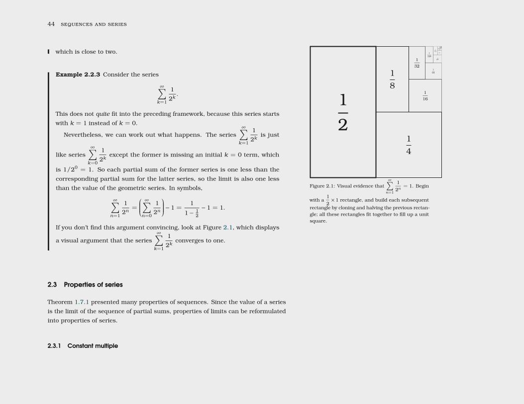
Figure 2.1: Visual evidence that∞∑n=1
12n
= 1. Begin
with a12× 1 rectangle, and build each subsequent
rectangle by cloning and halving the previous rectan-gle; all these rectangles fit together to fill up a unitsquare.
Example 2.2.3 Consider the series
∞∑k=1
12k
.
This does not quite fit into the preceding framework, because this series startswith k = 1 instead of k = 0.
Nevertheless, we can work out what happens. The series∞∑k=1
12k
is just
like series∞∑k=0
12k
except the former is missing an initial k = 0 term, which
is 1/20 = 1. So each partial sum of the former series is one less than thecorresponding partial sum for the latter series, so the limit is also one lessthan the value of the geometric series. In symbols,
∞∑n=1
12n
=
∞∑n=0
12n
− 1 =1
1 − 12− 1 = 1.
If you don’t find this argument convincing, look at Figure 2.1, which displays
a visual argument that the series∞∑k=1
12k
converges to one.
2.3 Properties of series
Theorem 1.7.1 presented many properties of sequences. Since the value of a seriesis the limit of the sequence of partial sums, properties of limits can be reformulatedinto properties of series.
2.3.1 Constant multiple
series 45
Theorem 2.3.1 Suppose∞∑k=0
ak is a convergent series, and c is a constant.
Then∞∑k=0
c ak converges, and
∞∑k=0
c ak = c∞∑k=0
ak .
Proof If you know just enough algebra to be dangerous, you may remember
that for any real numbers a, b, and c,
c(a + b) = c a + c b.
This is the distributive law for real numbers. By using the distributive law
more than once,
c(a0 + a1 + a2) = c a0 + c a1 + c a2,
or more generally, for some finite n,
c(a0 + a1 + a2 + · · ·+ an) = c a0 + c a1 + c a2 + · · ·+ c an .
So what’s the big deal with proving Theorem ? Can’t we just scream “distributive
law!” and be done with it? After all, Theorem amounts to
c a0 + c a1 + c a2 + · · ·+ c an + · · · = c(a0 + a1 + a2 + · · ·+ an + · · · ).
But hold your horses: you can only apply the distributive law finitely many
times! The distributive law, without some input from calculus, will not succeed
in justifying Theorem .
Let’s see how to handle this formally. By hypothesis,∞∑k=0
ak is a convergent
series, meaning its associated sequence of partial sums,
sn =n∑
k=0ak ,
46 sequences and series
converges. In other words, limn→∞
sn exists. Then, by Theorem ,
limn→∞
(c sn) = c limn→∞
sn .
But c sn is the sequence of partial sums for the series∞∑k=0
c ak , because
c sn = c a0 + c a1 + c a2 + · · ·+ c an .
Consequently,∞∑k=0
c ak = limn→∞
(c sn) = c limn→∞
sn ,
which is what we wanted to prove.
That theorem addresses the case of multiplying a convergent series by a constantc; what about divergence?
Example 2.3.2 Suppose that∞∑k=0
ak diverges; does∞∑k=0
c ak also diverge?
Solution If c = 0, then∞∑k=0
c ak =∞∑k=0
0 which does converge, to zero.
On the other hand, provided c , 0, then, yes,∞∑k=0
c ak also diverges. How
do we know?
We are working under the hypothesis that∞∑k=0
ak diverges. Suppose now, to
the contrary, that∞∑k=0
c ak did converge; applying Theorem 2.3.1 (albeit with
ak replaced by c ak and c replaced by (1/c)), the series
∞∑k=0
(1c
)c ak
series 47
converges, but that is ridiculous, since
∞∑k=0
(1c
)c ak =
∞∑k=0
ak
and the latter, under our hypothesis, diverged. A series cannot both converge
and diverge, so our assumption (that∞∑k=0
c ak did converge) must have been
mistaken—it must be that∞∑k=0
c ak diverges.
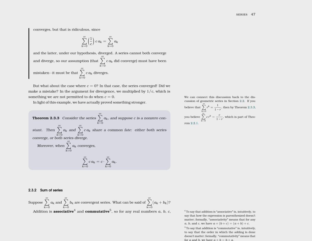
But what about the case where c = 0? In that case, the series converged! Did wemake a mistake? In the argument for divergence, we multiplied by 1/c, which issomething we are not permitted to do when c = 0. We can connect this discussion back to the dis-
cussion of geometric series in Section 2.2. If you
believe that∞∑k=0
rk =1
1 − r, then by Theorem 2.3.3,
you believe∞∑k=0
c rk =c
1 − r, which is part of Theo-
rem 2.2.1.
In light of this example, we have actually proved something stronger.
Theorem 2.3.3 Consider the series∞∑k=0
ak , and suppose c is a nonzero con-
stant. Then∞∑k=0
ak and∞∑k=0
c ak share a common fate: either both series
converge, or both series diverge.
Moreover, when∞∑k=0
ak converges,
∞∑k=0
c ak = c ·∞∑k=0
ak .
2.3.2 Sum of series
Suppose∞∑k=0
ak and∞∑k=0
bk are convergent series. What can be said of∞∑k=0
(ak + bk)?
Addition is associative4 and commutative5, so for any real numbers a, b, c, 4 To say that addition is “associative” is, intuitively, tosay that how the expression is parenthesized doesn’tmatter; formally, “associativity” means that for anya, b, and c, we have a + (b+ c) = (a + b) + c.5 To say that addition is “commutative” is, intuitively,to say that the order in which the adding is donedoesn’t matter; formally, “commutativity” means thatfor a and b, we have a + b = b+ a.
48 sequences and series
and d,(a + b) + (c + d) = (a + c) + (b+ d).
More generally, for real numbers a0, a1, a2, . . . , an and real numbers b0, b1, b2,. . . , bn,
(a0 +a1 +a2 + · · ·+an)+ (b0 +b1 +b2 + · · ·+bn) = (a0 +b0)+ (a1 +b1)+ (a2 +b2)+ · · ·+(an+bn).
But this finite statement can be beefed up into a statement about series. What wewant to prove is
∞∑k=0
ak +∞∑k=0
bk =∞∑k=0
(ak + bk) .
From above, we already know
n∑k=0
ak +n∑
k=0bk =
n∑k=0
(ak + bk) .
Take the limit of both sides.
limn→∞
n∑k=0
ak +n∑
k=0bk
= limn→∞
n∑k=0
(ak + bk) .
But the limit of a sum is the sum of the limits6, so 6 I like to call this a chiastic rule, since it has therhetorical pattern of a chiasmus. lim
n→∞
n∑k=0
ak
+ limn→∞
n∑k=0
bk
= limn→∞
n∑k=0
(ak + bk) .
Those three limits of partial sums can each be replaced by the series, which shows
∞∑k=0
ak +∞∑k=0
bk =∞∑k=0
(ak + bk) .
This can be summarized in a theorem.
series 49
Theorem 2.3.4 Suppose∞∑k=0
ak and∞∑k=0
bk are convergent series. Then
∞∑k=0
(ak + bk) is convergent, and
∞∑k=0
(ak + bk) =
∞∑k=0
ak
+ ∞∑k=0
bk
.
That covers sums of convergent series.
Example 2.3.5 Now suppose that∞∑k=0
ak and∞∑k=0
bk diverge; does∞∑k=0
(ak +bk)
diverge?
Solution Not necessarily. Let ak = 1 and bk = −1, so∞∑k=0
ak and∞∑k=0
bk
diverge. But
∞∑k=0
(ak + bk) =∞∑k=0
((1) + (−1)) =∞∑k=0
0 = 0.
This is not to say that the term-by-term sum of divergent series necessarily
converges, either. It is entirely possible that∞∑k=0
(ak + bk) will also diverge. For
istance, if ak = bk = 1, then
∞∑k=0
(ak + bk) =∞∑k=0
(1 + 1) =∞∑k=0
2
also diverges. So the term-by-term sum of divergent series might converge ormight diverge, depending on the situation.
50 sequences and series
2.4 Telescoping series
For most of this course, we will be happy if we can show that a series converges orthat a series diverges; we will not, usually, be too concerned with finding the valueof a series. Why not? Usually it is just too hard to determine the value; we would ifwe could, but since it is often too hard, we don’t bother.
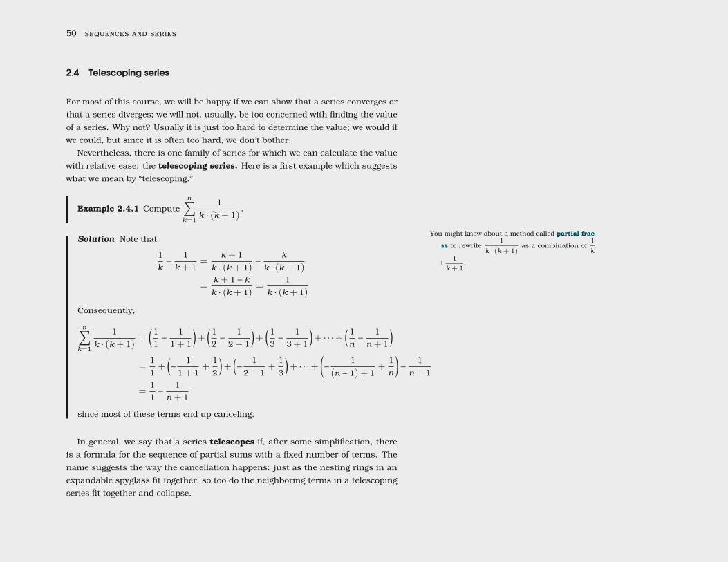
Nevertheless, there is one family of series for which we can calculate the valuewith relative ease: the telescoping series. Here is a first example which suggestswhat we mean by “telescoping.”
Example 2.4.1 Computen∑
k=1
1k · (k + 1)
.
You might know about a method called partial frac-
tions to rewrite1
k · (k + 1)as a combination of
1k
and1
k + 1.
Solution Note that
1k−
1k + 1
=k + 1
k · (k + 1)−
k
k · (k + 1)
=k + 1 − kk · (k + 1)
=1
k · (k + 1)
Consequently,
n∑k=1
1k · (k + 1)
=(11−
11 + 1
)+
(12−
12 + 1
)+
(13−
13 + 1
)+ · · ·+
(1n−
1n + 1
)=
11+
(−
11 + 1
+12
)+
(−
12 + 1
+13
)+ · · ·+
(−
1(n − 1) + 1
+1n
)−
1n + 1
=11−
1n + 1
since most of these terms end up canceling.
In general, we say that a series telescopes if, after some simplification, thereis a formula for the sequence of partial sums with a fixed number of terms. Thename suggests the way the cancellation happens: just as the nesting rings in anexpandable spyglass fit together, so too do the neighboring terms in a telescopingseries fit together and collapse.
series 51
Armed with a formula for the sequence of partial sums, we can attack thecorresponding infinite series.
Example 2.4.2 Compute∞∑k=1
1k · (k + 1)
.
Solution We just computed that
n∑k=1
1k · (k + 1)
= 1 −1
n + 1.
Rewriting the infinite series as the limit of the sequence of partial sums yields
∞∑k=1
1k · (k + 1)
= limn→∞
n∑k=1
1k · (k + 1)
= limn→∞
(1 −
1n + 1
)= lim
n→∞1 − lim
n→∞
1n + 1
= 1 − 0 = 1.
So the value of this series is 1.
2.5 A test for divergence
Usually, the sequence of partial sums sn = a0 + a1 + · · ·+ an is harder to under-stand and analyze than the sequence of terms ak . It would be helpful if we could saysomething about the complicated sequence sn by studying the easier-to-understandsequence ak .
Specifically, if the sequence sn converges, what can be said about the sequenceak? If adding up more and more terms from the sequence ak gets closer and closerto some number, then the size of the terms of ak had better be getting very small.Let’s make this precise.
52 sequences and series
Theorem 2.5.1 If∞∑k=0
ak converges then limn→∞
an = 0.
Proof Intuitively, this should seem reasonable: after all, if the terms in the
sequence an were getting very large (that is, not converging to zero), then adding
up those very large numbers would prevent the series∞∑k=0
ak from converging.
We can put this intuitive thinking on a firm foundation. Say∞∑k=0
ak con-
verges to L, meaning limn→∞
sn = L. But then also limn→∞
sn−1 = L, because that
sequence amounts to saying the same thing, but with the terms renumbered. By
Theorem ??,
limn→∞
(sn − sn−1) = limn→∞
sn − limn→∞
sn−1 = L − L = 0.
Replacing sn with a0 + · · ·+ an , we get
sn − sn−1 = (a0 + a1 + a2 + · · ·+ an) − (a0 + a1 + a2 + · · ·+ an−1) = an ,
and therefore, limn→∞
an = 0.
The contrapositive of Theorem 2.5.1 can be used as a divergence test.
Theorem 2.5.2 Consider the series∞∑k=0
ak . If the limit limn→∞
an does not exist
or has a value other than zero, then the series diverges.
We’ll usually call this theorem the “nth term test.”
Warning The converse of Theorem 2.5.1 is not true: even if limn→∞
an = 0, theseries could diverge.
series 53
This is a very common mistake: you might be tempted to show that a seriesconverges by showing lim
n→∞an = 0, but that doesn’t work. The nth term test
either says “diverges!” or says nothing at all. It is not possible to show thatanything converges by using the nth term test.
For an example, see Section 2.6.
One analogy that can be helpful is think about weather: whenever it is raining, itis cloudy. Yet it is possible for there to be clouds, even on a rainless day. 7 7 We first introduced this idea on Page 24.
Likewise, whenever the series∞∑k=0
ak converges (“it is raining”), the sequence
ak converges to zero (“it is cloudy”). If it isn’t cloudy, then we can be sure it isn’training—and this is the statement of Theorem 2.5.2. Let’s use this “divergence test”to show that a particular series diverges.
Example 2.5.3 Show that∞∑n=1
n
n + 1diverges.
Solution We apply the nth term test: all we need to do is to compute the limit
limn→∞
n
n + 1= 1 , 0.
Since the limit exists but is not zero (i.e., “it is not cloudy”), the series mustdiverge (“it can’t be raining.”).
Looking at the first few terms perhaps makes it clear that the series has nochance of converging:
12+
23+
34+
45+ · · ·
will just get larger and larger; indeed, after a bit longer the series starts tolook very much like · · ·+ 1 + 1 + 1 + 1 + · · · , and if we add up many numberswhich are very close to one, then we can make the sum as large as we desire.
54 sequences and series
2.6 Harmonic series
The series∞∑n=1
1n
has a special name.
Definition The series
∞∑n=1
1n=
11+
12+
13+
14+ · · ·
is called the harmonic series.
The main question for this section—indeed, the question which should always beour first question anytime we see an unknown series—is the following question:
Does the harmonic series converge. . . or diverge?
How can we begin to explore this question?
2.6.1 The limit of the termsWhen confronted with the question of whether aseries diverges or converges, the first thing to checkis the limit of the terms—if that limit doesn’t exist,or does exist but equals a number other than zero,then the series diverges.
In general, the easiest way to prove that a series diverges is to apply the nth termtest from Theorem 2.5.2. What does the nth term test tell us for the harmonic series?We calculate
limn→∞
1n= 0,
so the nth term test is silent; since the limit of the terms of the series exists and isequal to zero, the nth term test does not tell us any information.
The harmonic series passed the first gauntlet—but that does not mean theharmonic series will survive the whole game. All we know is that the harmonic doesdoesn’t diverge for the most obvious reason, but whether it diverges or converges isyet to be determined.
2.6.2 Numerical evidence
If you have the fortitude8 to add up the first hundred terms, you will find that 8 lacking fortitude, software will suffice
series 55
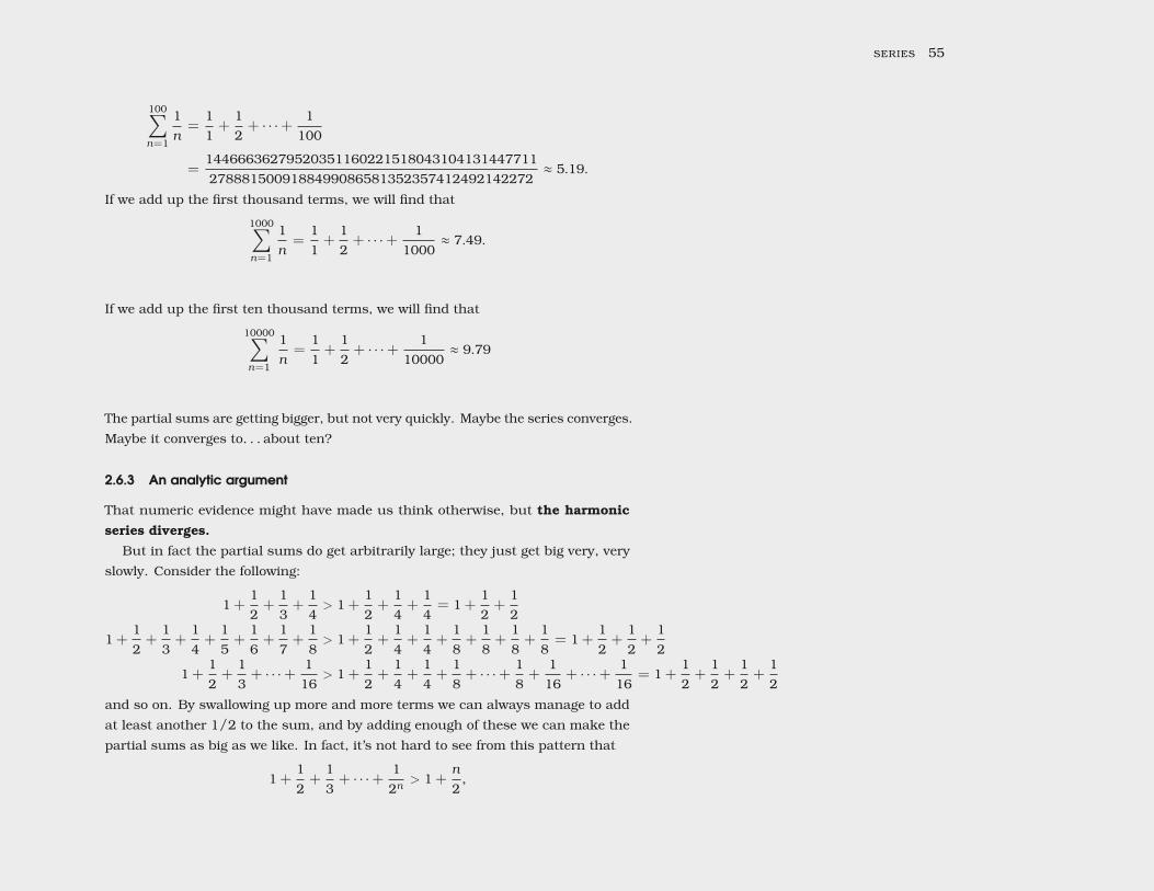
100∑n=1
1n=
11+
12+ · · ·+
1100
=144666362795203511602215180431041314477112788815009188499086581352357412492142272
≈ 5.19.
If we add up the first thousand terms, we will find that
1000∑n=1
1n=
11+
12+ · · ·+
11000
≈ 7.49.
If we add up the first ten thousand terms, we will find that
10000∑n=1
1n=
11+
12+ · · ·+
110000
≈ 9.79
The partial sums are getting bigger, but not very quickly. Maybe the series converges.Maybe it converges to. . . about ten?
2.6.3 An analytic argument
That numeric evidence might have made us think otherwise, but the harmonic
series diverges.
But in fact the partial sums do get arbitrarily large; they just get big very, veryslowly. Consider the following:
1 +12+
13+
14> 1 +
12+
14+
14= 1 +
12+
12
1 +12+
13+
14+
15+
16+
17+
18> 1 +
12+
14+
14+
18+
18+
18+
18= 1 +
12+
12+
12
1 +12+
13+ · · ·+
116
> 1 +12+
14+
14+
18+ · · ·+
18+
116
+ · · ·+116
= 1 +12+
12+
12+
12
and so on. By swallowing up more and more terms we can always manage to addat least another 1/2 to the sum, and by adding enough of these we can make thepartial sums as big as we like. In fact, it’s not hard to see from this pattern that
1 +12+
13+ · · ·+
12n
> 1 +n
2,
56 sequences and series
so to make sure the sum is over 100, for example, we’d add up terms until we get toaround 1/2198, that is, about 4 · 1059 terms.
2.7 Comparison test
A bounded, monotonic sequence necessarily converges (Theorem 1.8.2). How doesthis fact about sequences relate to series? When is the sequence of partial sumsmonotonic? If the terms of a series are non-negative, then the associated sequenceof partial sums is non-decreasing.
Corollary 2.7.1 Consider the series∞∑k=0
ak . Assume the terms ak are non-
negative. If the sequence of partial sums sn = a0 + · · ·+ an is bounded, thenthe series converges.
So we can show that a series of positive terms converges, provided we can boundthe sequence of partial sums.
2.7.1 Statement of the Comparison Test
But how can we manage to do that? One way to ensure that the sequence of partialsums is bounded is by comparing the series to another series. Consider two series
∞∑k=0
ak and∞∑k=0
bk .
Suppose, for all k, that bk ≥ ak ≥ 0. Then
a0 + a1 + · · ·+ an ≤ b0 + b1 + · · ·+ bn .
Suppose that∞∑k=0
bk converges to L. Then
a0 + a1 + · · ·+ an ≤ b0 + b1 + · · ·+ bn ≤ L,
series 57
so the sequence of partial sums sn = a0 + a1 + · · ·+ an is bounded. But we just won
the game: each term ak is nonnegative, so the sequence of partial sums sn =n∑
k=0ak
is increasing. Theorem 1.8.2 guarantees that the sequence (sn) converges.Let’s summarize what just happened: if a series with positive terms is, termwise,
less than a convergent series, it converges. We have just proved half of the followingtheorem.
Theorem 2.7.2 Suppose that an and bn are non-negative for all n and that,for some N , whenever n ≥ N , we have an ≤ bn.
If∞∑n=0
bn converges, so does∞∑n=0
an.
If∞∑n=0
an diverges, so does∞∑n=0
bn.
This is usually called the Comparison Test; we might summarize it like this:
• A non-negative series, overestimated by a convergent series, converges.
• A non-negative series, underestimated by a divergent series, diverges.
Warning Being less than a divergent series does not help: the comparison testis silent in that case.
Similarly, being larger than a convergent series does not help. The Compari-son Test only says something when a series (with non-negative terms!) is lessthan a convergent series, or greater than a divergent series.
2.7.2 Applications of the Comparison Test
Like the nth term test (Theorem 2.5.2), we can use the Comparison Test (Theo-rem 2.7.2) to show that a series diverges.
58 sequences and series
Example 2.7.3 Does the series∞∑n=2
lognn
converge?
Solution Our first inclination might be to apply the nth term test, but in thiscase,
limn→∞
lognn
= 0,
so the nth term test is silent in this case. As far as we know at this point, theseries may diverge or converge.
Instead, we’ll try the Comparison Test. Set an =1n
and bn =lognn
. Notethat whenever n ≥ 3, we have
0 ≤ an ≤ bn ,
but the series∞∑n=3
1n
diverges, and so by the Comparison Test, the given series
(which is even bigger!) must likewise diverge.
Recall that the nth term test cannot be used to prove that a series converges; ifthe nth term test does not answer “diverges!” then the test is silent. In wonderfulcontrast, the Comparison Test can be used to show that a series converges.
Example 2.7.4 Does the series∞∑n=1
sin2 n
2nconverge?
Solution Yes. Set
an =sin2 n
2nand bn =
12n
Note that 0 ≤ an ≤ bn . But the series∞∑n=1
bn converges, since it is a geometric
series with common ratio 1/2, as in Example 2.2.2. Therefore, the series∞∑n=1
an converges by the comparison test.
series 59
2.7.3 Cauchy Condensation TestIf you have already seen some convergence testsbefore—perhaps you have already been through Cal-culus Two!—you might be wondering why “conden-sation” is making an appearance. It is perhaps lesspopular than other tests, but I like it. Pedagogically,it is nice to see that the “trick” in the harmonic seriescan be generalized and applied to lots of other series.In particular, condensation permits the study of p-series without going through the usual route of theIntegral Test.
Remember in Section 2.6 when we considered the harmonic series? We showed
that it diverged by comparing it with the divergent series∞∑n=1
12
, but we couldn’t
make that comparison right away—first we had to group together the terms in asomewhat complicated seeming way.
We can generalize that “grouping together” trick; this is called the CauchyCondensation Test.
Theorem 2.7.5 Suppose (an) is a non-increasing sequence of positive num-
bers. The series∞∑n=1
an converges if and only if the series∞∑n=0
(2na2n ) converges.
The series∞∑n=0
(2na2n ) is often called the condensed series associated to the
series∞∑n=1
an.
Proof Let’s suppose that∞∑n=0
(2na2n ) converges; the goal then is to show that
∞∑n=1
an also converges.
Since the sequence (an) is decreasing, we have that
a2 + a3 ≤ a2 + a2
a4 + a5 + a6 + a7 ≤ a4 + a4 + a4 + a4
a8 + · · ·+ a15 ≤ 8a8
...
a2n + · · ·+ a2n+1−1 ≤ 2n a2n .
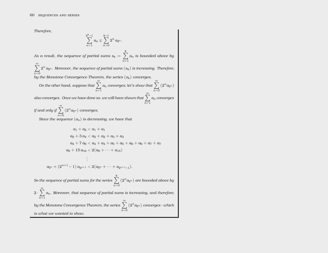
60 sequences and series
Therefore,2k−1∑n=1
an ≤k−1∑n=0
2n a2n .
As a result, the sequence of partial sums sk =k∑
n=1an is bounded above by
∞∑n=0
2n a2n . Moreover, the sequence of partial sums (sk) is increasing. Therefore,
by the Monotone Convergence Theorem, the series (sk) converges.
On the other hand, suppose that∞∑n=1
an converges; let’s show that∞∑n=0
(2na2n )
also converges. Once we have done so, we will have shown that∞∑n=1
an converges
if and only if∞∑n=0
(2na2n ) converges.
Since the sequence (an) is decreasing, we have that
a1 + a2 < a1 + a1
a2 + 3a4 < a2 + a2 + a3 + a3
a4 + 7a8 < a4 + a4 + a5 + a5 + a6 + a6 + a7 + a7
a8 + 15a16 < 2(a8 + · · ·+ a15)
...
a2n + (2n+1 − 1) a2n+1 < 2(a2n + · · ·+ a2n+1−1).
So the sequence of partial sums for the seriesk∑
n=0(2na2n ) are bounded above by
2 ·∞∑n=1
an . Moreover, that sequence of partial sums is increasing, and therefore,
by the Monotone Convergence Theorem, the series∞∑n=0
(2na2n ) converges—which
is what we wanted to show.
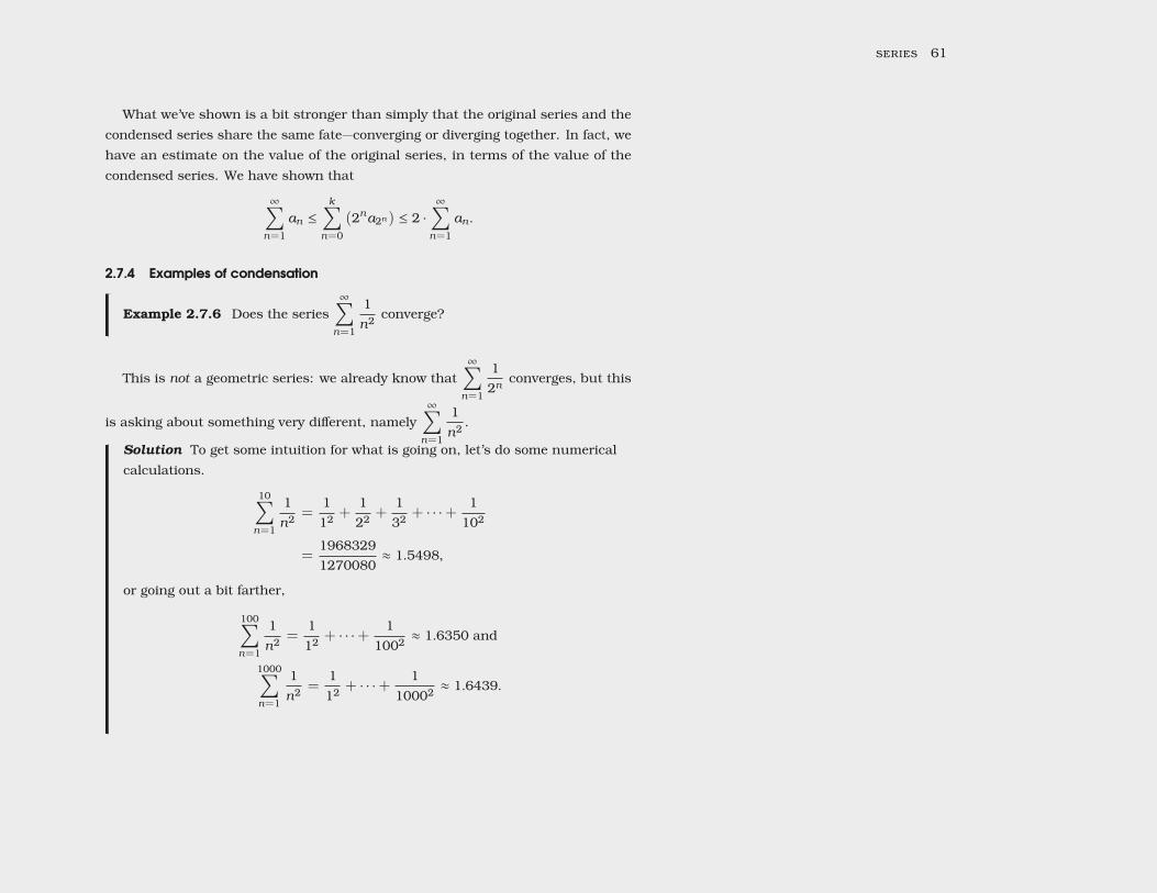
series 61
What we’ve shown is a bit stronger than simply that the original series and thecondensed series share the same fate—converging or diverging together. In fact, wehave an estimate on the value of the original series, in terms of the value of thecondensed series. We have shown that
∞∑n=1
an ≤k∑
n=0(2na2n ) ≤ 2 ·
∞∑n=1
an .
2.7.4 Examples of condensation
Example 2.7.6 Does the series∞∑n=1
1n2 converge?
This is not a geometric series: we already know that∞∑n=1
12n
converges, but this
is asking about something very different, namely∞∑n=1
1n2 .
Solution To get some intuition for what is going on, let’s do some numericalcalculations.
10∑n=1
1n2 =
112 +
122 +
132 + · · ·+
1102
=19683291270080
≈ 1.5498,
or going out a bit farther,
100∑n=1
1n2 =
112 + · · ·+
11002 ≈ 1.6350 and
1000∑n=1
1n2 =
112 + · · ·+
110002 ≈ 1.6439.
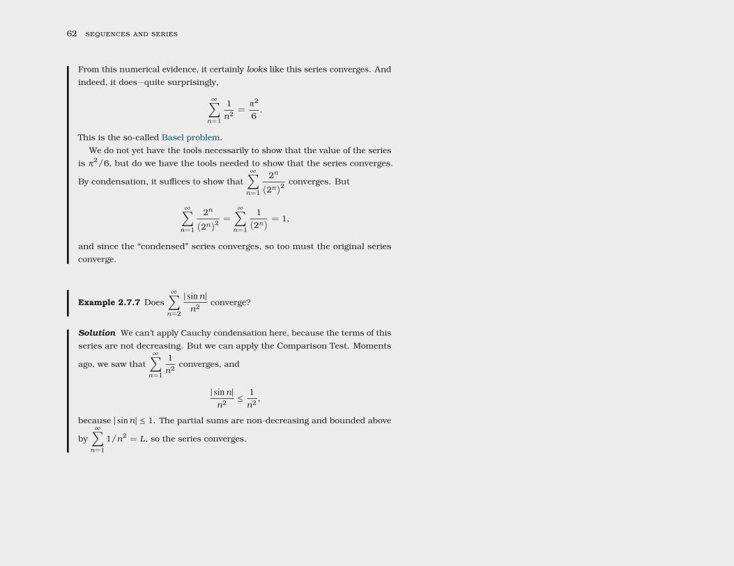
62 sequences and series
From this numerical evidence, it certainly looks like this series converges. Andindeed, it does—quite surprisingly,
∞∑n=1
1n2 =
π2
6.
This is the so-called Basel problem.We do not yet have the tools necessarily to show that the value of the series
is π2/6, but do we have the tools needed to show that the series converges.
By condensation, it suffices to show that∞∑n=1
2n
(2n)2 converges. But
∞∑n=1
2n
(2n)2 =∞∑n=1
1(2n)
= 1,
and since the “condensed” series converges, so too must the original seriesconverge.
Example 2.7.7 Does∞∑n=2
| sinn|n2 converge?
Solution We can’t apply Cauchy condensation here, because the terms of thisseries are not decreasing. But we can apply the Comparison Test. Moments
ago, we saw that∞∑n=1
1n2 converges, and
| sinn|n2 ≤
1n2 ,
because | sinn| ≤ 1. The partial sums are non-decreasing and bounded above
by∞∑n=1
1/n2 = L, so the series converges.
series 63
2.7.5 Convergence of p-series
Let us consider the series∞∑n=1
1np
. Such a series is called a p-series. Does a p-series
converge? Diverge? It depends on p. If we think of this as a function of p, then we havethe Riemann zeta function, that is,
ζ (p) =∞∑n=1
1np
.
The Riemann zeta function is quite important: itplays a key role in number theory via the Riemannhypothesis and also has applications in physics.Something that connects the physical world to num-ber theory must be pretty incredible.
Example 2.7.8 Let p ≤ 1. Does the series∞∑n=1
1np
converge?
Solution When p = 1, this series is the harmonic series we already proved todiverge in Section 2.6.
But more generally, the series∞∑n=1
1np
diverges whenever p ≤ 1. We will
show this by comparing to a harmonic series. Since p ≤ 1, then np ≤ n, and so
1np≥
1n
.
But the harmonic series∞∑n=1
1n
diverges, and so by comparison, the series
∞∑n=1
1np
diverges.
Example 2.7.9 Let p > 1. Does the series∞∑n=1
1np
converge?
Solution It converges. For this, we use Cauchy condensation: consider the“condensed” series
∞∑n=1
2n ·1
(2n)p.
But this series simplifies to
∞∑n=1
2n ·1
(2n)p=
∞∑n=1
1(2p−1)n
,

64 sequences and series
which converges.

series 65
Exercises for Section 2.7
(1) Explain why∞∑n=1
n2
2n2 + 1diverges. à
(2) Explain why∞∑n=1
521/n + 14
diverges. à
(3) Explain why∞∑n=1
3n
diverges. à
(4) Compute∞∑n=0
4(−3)n
−33n
. à
(5) Compute∞∑n=0
32n
+45n
. à
(6) Compute∞∑n=0
4n+1
5n. à
(7) Compute∞∑n=0
3n+1
7n+1 . à
(8) Compute∞∑n=1
(35
)n. à
(9) Compute∞∑n=1
3n
5n+1 . à

3 Convergence tests
It is generally quite difficult—indeed, often impossible—to determine the value of aseries exactly. Even if we can’t compute the value of a series, in many cases it ispossible to determine whether or not the series converges. We will spend most ofour time on this problem.
3.1 Ratio tests
Does the series∞∑n=0
n5
5nconverge? It is possible, but a bit unpleasant, to approach
this with the comparison test. Mathematics is more than just about getting an-swers; a goal of mathematics is not only to findtruth, but to package the resulting “truth” in a for-mat that permits another human being to under-stand the reasons for its being true. Arguments likethis—which are perfectly convincing but seem en-tirely unmotivated—are, arguably, missing the point.What has been gained if we find something is true butthe reason for its being true remains inscrutable?
Example 3.1.1 The series∞∑n=0
n5
5nconverges.
This idea—that the first handful of terms do notaffect convergence at all—will be discussed formallyin Section 5.1.
Solution As long as n ≥ 23, we have 2n ≥ n5. Therefore, as long as n ≥ 23,we have
n5
5n≤
2n
5n=
(25
)nBut the geometric series
∞∑n=23
(25
)nconverges, since the ratio between subse-
quent terms is less than one. So by comparison, the smaller series
∞∑n=23
n5
5n
68 sequences and series
must also converge. The first handful of terms when n < 23 doesn’t affectconvergence at all, so we are justified to conclude that the original series∞∑n=0
n5
5nconverges.
That worked—but it invoked an unmotivated fact: how do I know that 2n ≥ n5
whenever n ≥ 23? Invoking that fact seems a bit random—yes, yes, a proof, butperhaps not a proof that conveys exactly what is going on. It is a valid argument,but missing some motivation.
3.1.1 Theory
Instead, consider what happens as we move from one term to the next term in thisseries, that is, consider two neighboring terms
· · ·+n5
5n+
(n + 1)5
5n+1 + · · · .
The denominator goes up by a factor of 5, 5n+1 = 5 · 5n , but the numerator goes upby much less: (n + 1)5 = n5 + 5n4 + 10n3 + 10n2 + 5n + 1, which is much lessthan 5n5 when n is large, because 5n4 is much less than n5. (This sort of thinkingis why it was worth comparing n5 to an exponential 2n for n large.)
So we might guess that in the long run—when n is very large—it begins to look asif each term is about 1/5 of the previous term. We have seen series that behavelike this, namely the geometric series
∞∑n=0
15n
=54
.
We are beginning to see why it made sense to compare the given series to a geometricseries as in the initially very unmotivated argument above.
But we can do better! Instead of an ad hoc argument which compared n5 to 2n,we can try to make rigorous the idea that each term is “eventually” about a fifth asbig as the previous term. The key is to notice that
limn→∞
an+1
an= lim
n→∞
(n + 1)5
5n+15n
n5 = limn→∞
(n + 1)5
n515= 1 ·
15=
15
.
convergence tests 69
This is a more formal version of what we noticed about the ratio of subsequentterms: in the long run, each term is one fifth of the previous term. Pick some
number just slightly bigger than15
; let’s call that number15+ ε. The symbol ε is the Greek letter epsilon, and, con-
ventionally, denotes a small but positive number.Becauselimn→∞
an+1
an=
15
,
then by choosing n big enough, say n ≥ N for some N , we can guarantee thatan+1
an
is as close as we’d like to15
, say within ε of15
. More succinctly, there must be someN so that whenever n ≥ N , we have
an+1
an<
15+ ε
Multiplying both sides by an, we find whenever n ≥ N that
an+1 <(15+ ε
)an .
We can say the same thing when n is replaced by N + 1, meaning
aN+2 <(15+ ε
)aN+1,
which together with the previous statement when n is N implies
aN+2 <(15+ ε
)2aN .
And we can repeat this again! Since
aN+3 <(15+ ε
)aN+2,
we also learn that
aN+3 <(15+ ε
)3aN ,
or in general,
aN+k <(15+ ε
)kaN .
This is setting up a comparison. The geometric series
∞∑k=0
(15+ ε
)kaN =
∞∑k=0
(15+ ε
)kaN

70 sequences and series
converges as long as ε had been chosen so small that15+ ε < 1. But if that series
converges, then the series
∞∑k=0
aN+k = aN + aN+1 + aN+2 + · · ·
also converges, because each term of that series is smaller than the correspondingterm of the convergent geometric series. But if that series converges, then
∞∑k=0
ak = a0 + a1 + a2 + · · ·
converges since we’ve just added the number a0 + a1 + · · ·+ aN−1 to the convergent
series∞∑k=0
aN+k .
Under what circumstances could we do this? What was crucial was that the limitof an+1/an , say L, was less than 1 so that we could pick a value ε so that L + ε < 1and then compare to the convergent series
∞∑k=0
(L + ε)k · aN .
That’s really all that is required to make the argument work. We also made use ofthe fact that the terms of the series were positive. Let’s summarize the situation In general, we can consider instead the absolute
values of the terms, and end up testing for absoluteconvergence. We’ll discuss this topic in Section 4.1.
when this works.
Theorem 3.1.2 (The Ratio Test) Consider the series∞∑n=0
an where each term
an is positive. Suppose that
limn→∞
an+1
an= L.
If L < 1 the series∞∑n=0
an converges. If L > 1 the series diverges. If L = 1 this
test is inconclusive.
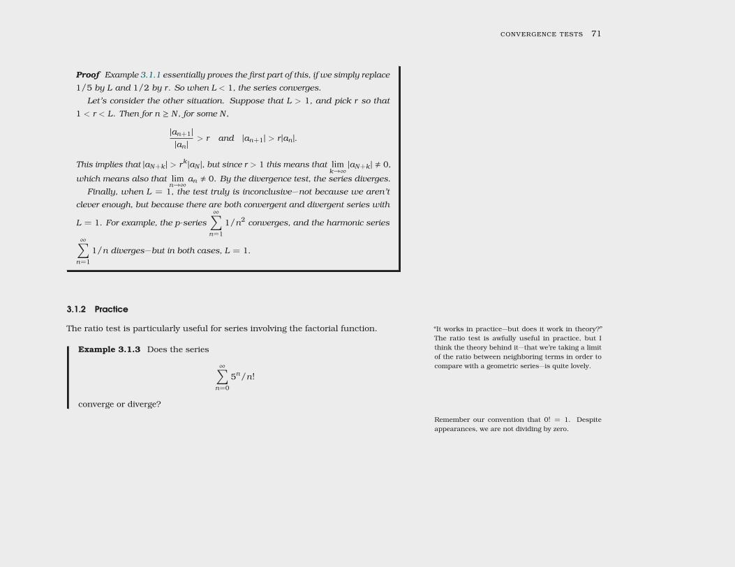
convergence tests 71
Proof Example 3.1.1 essentially proves the first part of this, if we simply replace
1/5 by L and 1/2 by r. So when L < 1, the series converges.
Let’s consider the other situation. Suppose that L > 1, and pick r so that
1 < r < L. Then for n ≥ N , for some N ,
|an+1|
|an |> r and |an+1| > r |an |.
This implies that |aN+k | > rk |aN |, but since r > 1 this means that lim
k→∞|aN+k | , 0,
which means also that limn→∞
an , 0. By the divergence test, the series diverges.
Finally, when L = 1, the test truly is inconclusive—not because we aren’t
clever enough, but because there are both convergent and divergent series with
L = 1. For example, the p-series∞∑n=1
1/n2 converges, and the harmonic series
∞∑n=1
1/n diverges—but in both cases, L = 1.
3.1.2 Practice
The ratio test is particularly useful for series involving the factorial function. “It works in practice—but does it work in theory?”The ratio test is awfully useful in practice, but Ithink the theory behind it—that we’re taking a limitof the ratio between neighboring terms in order tocompare with a geometric series—is quite lovely.
Example 3.1.3 Does the series
∞∑n=0
5n/n!
converge or diverge?
Remember our convention that 0! = 1. Despiteappearances, we are not dividing by zero.
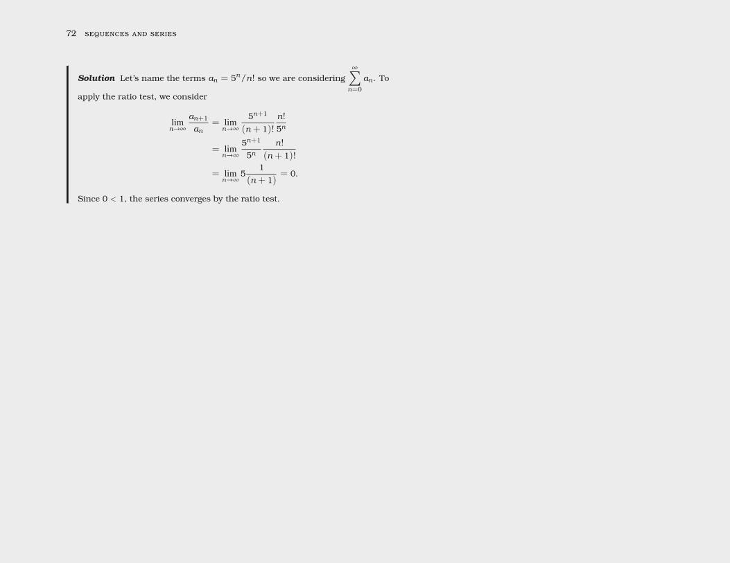
72 sequences and series
Solution Let’s name the terms an = 5n/n! so we are considering∞∑n=0
an. To
apply the ratio test, we consider
limn→∞
an+1
an= lim
n→∞
5n+1
(n + 1)!n!5n
= limn→∞
5n+1
5nn!
(n + 1)!
= limn→∞
51
(n + 1)= 0.
Since 0 < 1, the series converges by the ratio test.
convergence tests 73
Exercises for Section 3.1
(1) Compute limn→∞
|an+1/an | for the series∞∑n=1
1n2 . à
(2) Compute limn→∞
|an+1/an | for the series∞∑n=1
1n
. à
Determine whether each of the following series converges or diverges.
(3)∞∑n=0
(−1)n3n
5n à
(4)∞∑n=1
n!nn à
(5)∞∑n=1
n5
nn à
(6)∞∑n=1
(n!)2
nn à
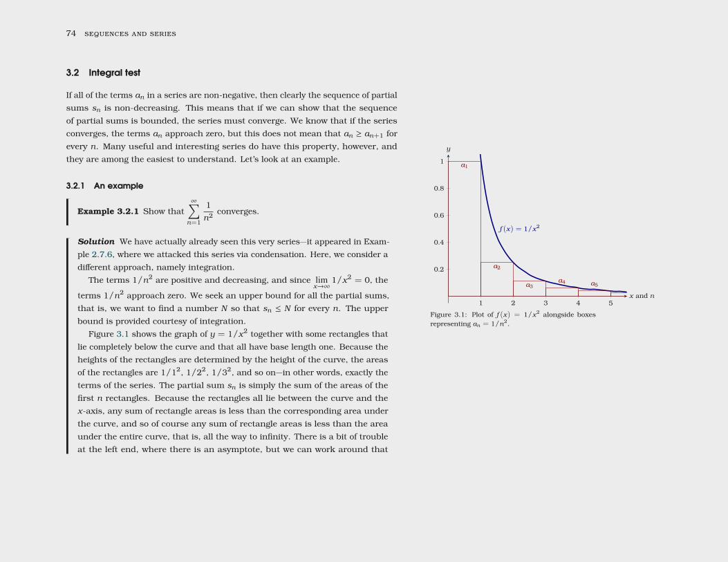
74 sequences and series
3.2 Integral test
If all of the terms an in a series are non-negative, then clearly the sequence of partialsums sn is non-decreasing. This means that if we can show that the sequenceof partial sums is bounded, the series must converge. We know that if the seriesconverges, the terms an approach zero, but this does not mean that an ≥ an+1 forevery n. Many useful and interesting series do have this property, however, andthey are among the easiest to understand. Let’s look at an example.
3.2.1 An example
Example 3.2.1 Show that∞∑n=1
1n2 converges.
1 2 3 4 5
0.2
0.4
0.6
0.8
1
f (x) = 1/x2
a1
a2
a3a4 a5
x and n
y
Figure 3.1: Plot of f (x) = 1/x2 alongside boxesrepresenting an = 1/n2.
Solution We have actually already seen this very series—it appeared in Exam-ple 2.7.6, where we attacked this series via condensation. Here, we consider adifferent approach, namely integration.
The terms 1/n2 are positive and decreasing, and since limx→∞
1/x2 = 0, the
terms 1/n2 approach zero. We seek an upper bound for all the partial sums,that is, we want to find a number N so that sn ≤ N for every n. The upperbound is provided courtesy of integration.
Figure 3.1 shows the graph of y = 1/x2 together with some rectangles thatlie completely below the curve and that all have base length one. Because theheights of the rectangles are determined by the height of the curve, the areasof the rectangles are 1/12, 1/22, 1/32, and so on—in other words, exactly theterms of the series. The partial sum sn is simply the sum of the areas of thefirst n rectangles. Because the rectangles all lie between the curve and thex-axis, any sum of rectangle areas is less than the corresponding area underthe curve, and so of course any sum of rectangle areas is less than the areaunder the entire curve, that is, all the way to infinity. There is a bit of troubleat the left end, where there is an asymptote, but we can work around that
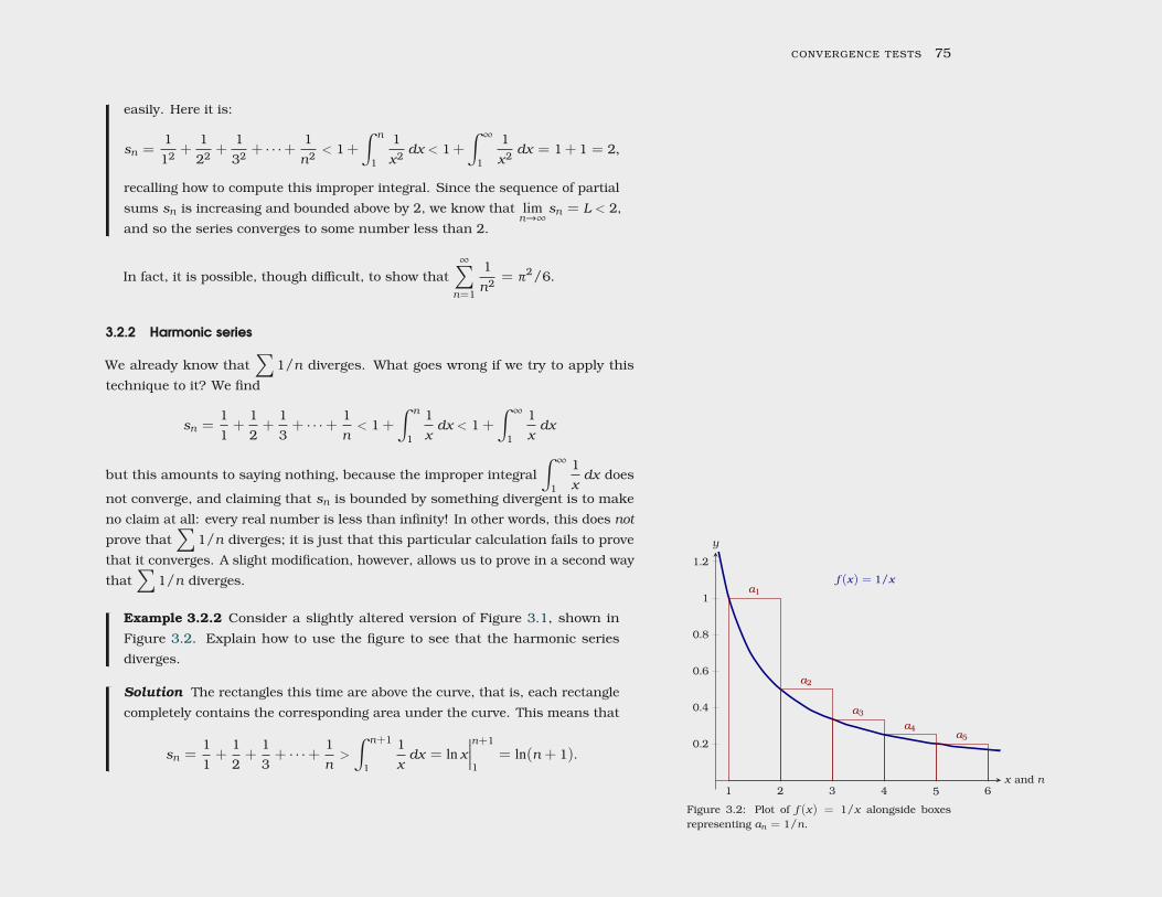
convergence tests 75
easily. Here it is:
sn =112 +
122 +
132 + · · ·+
1n2 < 1+
∫ n
1
1x2 dx < 1+
∫ ∞
1
1x2 dx = 1+ 1 = 2,
recalling how to compute this improper integral. Since the sequence of partialsums sn is increasing and bounded above by 2, we know that lim
n→∞sn = L < 2,
and so the series converges to some number less than 2.
In fact, it is possible, though difficult, to show that∞∑n=1
1n2 = π2/6.
3.2.2 Harmonic series
We already know that∑
1/n diverges. What goes wrong if we try to apply thistechnique to it? We find
sn =11+
12+
13+ · · ·+
1n< 1 +
∫ n
1
1xdx < 1 +
∫ ∞
1
1xdx
but this amounts to saying nothing, because the improper integral∫ ∞
1
1xdx does
not converge, and claiming that sn is bounded by something divergent is to makeno claim at all: every real number is less than infinity! In other words, this does not
prove that∑
1/n diverges; it is just that this particular calculation fails to provethat it converges. A slight modification, however, allows us to prove in a second waythat
∑1/n diverges.
Example 3.2.2 Consider a slightly altered version of Figure 3.1, shown inFigure 3.2. Explain how to use the figure to see that the harmonic seriesdiverges.
1 2 3 4 5 6
0.2
0.4
0.6
0.8
1
1.2f (x) = 1/x
a1
a2
a3a4
a5
x and n
y
Figure 3.2: Plot of f (x) = 1/x alongside boxesrepresenting an = 1/n.
Solution The rectangles this time are above the curve, that is, each rectanglecompletely contains the corresponding area under the curve. This means that
sn =11+
12+
13+ · · ·+
1n>
∫ n+1
1
1xdx = ln x
∣∣∣∣∣n+1
1= ln(n + 1).
76 sequences and series
As n gets bigger, ln(n + 1) goes to infinity, so the sequence of partial sums snmust also go to infinity, so the harmonic series diverges.
3.2.3 Statement of integral test
The important fact that clinches this example is that
limn→∞
∫ n+1
1
1xdx = ∞,
which we can rewrite as ∫ ∞
1
1xdx = ∞.
So these two examples taken together indicate that we can prove that a seriesconverges or prove that it diverges with a single calculation of an improper integral.This is known as the integral test, which we state as a theorem.
Theorem 3.2.3 (Integral test) Suppose that f (x) > 0 and is decreasing onthe infinite interval [k,∞) (for some k ≥ 1) and that an = f (n). Then the series∞∑n=k
an converges if and only if the improper integral∫ ∞
kf (x) dx converges.
3.2.4 p-series
The two examples we have seen are examples of p-series, which we first encountered
in Subsection 2.7.5. Recall that a p-series is any series of the form∞∑n=1
1/np.
Theorem 3.2.4 A p-series converges if and only if p > 1.
We already proved this theorem using condensation in Example 2.7.8 andExample 2.7.9. Nevertheless, we provide a second proof, using the integral test.
convergence tests 77
Proof We use the integral test; the case p = 1 is that of the harmonic series,
which we know diverges, so without loss of generality, we may assume that
p , 1. If p ≤ 0, limn→∞
1/np , 0, so the series diverges by Theorem 2.5.2. So we
may also assume that p > 0.
Then we compute∫ ∞
1
1xpdx = lim
N→∞
x1−p
1 − p
∣∣∣∣∣∣N1= lim
N→∞
N1−p
1 − p−
11 − p
.
If p > 1 then 1−p < 0 and limN→∞
N1−p = 0, so the integral converges. If 0 < p < 1
then 1 − p > 0 and limN→∞
N1−p = ∞, so the integral diverges.
Example 3.2.5 Show that∞∑n=1
1n3 converges.
Solution We could of course use the integral test, but now that we have thetheorem we may simply note that this is a p-series with p = 3 > 1.
Example 3.2.6 Show that∞∑n=1
5n4 converges.
Solution We know that if∞∑n=1
1/n4 converges then∞∑n=1
5/n4 also converges,
by Theorem 2.3.1. Since∞∑n=1
1/n4 is a convergent p-series,∞∑n=1
5/n4 converges
also.
Example 3.2.7 Show that∞∑n=1
5√n
diverges.
78 sequences and series
Solution This also follows from Theorem 2.3.4. Since∞∑n=1
1√n
is a p-series
with p = 1/2 < 1, it diverges, and so does∞∑n=1
5√n
.
3.2.5 Integrating for approximations
Since it is typically difficult to compute the value of a series exactly, a good approx-imation is frequently required. In a real sense, a good approximation is only asgood as we know it is, that is, while an approximation may in fact be good, it isonly valuable in practice if we can guarantee its accuracy to some degree1. This 1 After all, π ≈ 17 just with very bad error bounds.
It is better to make a statement like |π − 17| < 14,which is not only saying that π is “close” to 17, but isquantifying exactly how close (within 14—so perhapsnot all that close).
guarantee is usually easy to come by for series with decreasing positive terms.
Example 3.2.8 Approximate∞∑n=1
1/n2 to two decimal places.
It turns out that∞∑n=1
1n2 =
π2
6, so your approxima-
tion of this series will also—in a roundabout way—yield an approximate value for π—and one which willbe better than 17.
Solution Referring to Figure 3.1, if we approximate the sum byN∑n=1
1/n2,
the error we make is the total area of the remaining rectangles, all of whichlie under the curve 1/x2 from x = N out to infinity. So we know the truevalue of the series is larger than the approximation, and no bigger than theapproximation plus the area under the curve from N to infinity. Roughly, then,we need to find N so that ∫ ∞
N
1x2 dx < 1/100.
We can compute the integral: ∫ ∞
N
1x2 dx =
1N
,
so N = 100 is a good starting point. Adding up the first 100 terms gives approx-imately 1.634983900, and that plus 1/100 is 1.644983900, so approximatingthe series by the value halfway between these will be at most 1/200 = 0.005
convergence tests 79
in error. The midpoint is 1.639983900, but while this is correct to ±0.005, wecan’t tell if the correct two-decimal approximation is 1.63 or 1.64. We need tomake N big enough to reduce the guaranteed error, perhaps to around 0.004 tobe safe, so we would need 1/N ≈ 0.008, or N = 125. Now the sum of the first125 terms is approximately 1.636965982, and that plus 0.008 is 1.644965982and the point halfway between them is 1.640965982. The true value is then1.640965982 ± 0.004, and all numbers in this range round to 1.64, so 1.64 iscorrect to two decimal places.
Since∞∑n=1
1n2 =
π2
6, our estimate yields
1.63 <π2
6< 1.65,
and so9.78 < π2 < 9.90.
which means that3.127 < π < 3.147,
which is better than π ≈ 3. And we have explicit bounds on the error.
80 sequences and series
Exercises for Section 3.2
Determine whether each series converges or diverges.
(1)∞∑n=1
1nπ/4 à
(2)∞∑n=1
n
n2 + 1 à
(3)∞∑n=1
lnnn2 à
(4)∞∑n=1
1n2 + 1 à
(5)∞∑n=1
1en à
(6)∞∑n=1
n
en à
(7)∞∑n=2
1n lnn à
(8)∞∑n=2
1n(lnn)2 à
(9) Find an N so that∞∑n=1
1n4 is between
N∑n=1
1n4 and
N∑n=1
1n4 + 0.005. à
(10) Find an N so that∞∑n=0
1en
is betweenN∑n=0
1en
andN∑n=0
1en
+ 10−4. à
(11) Find an N so that∞∑n=1
lnnn2 is between
N∑n=1
lnnn2 and
N∑n=1
lnnn2 + 0.005. à
(12) Find an N so that∞∑n=2
1n(lnn)2 is between
N∑n=2
1n(lnn)2 and
N∑n=2
1n(lnn)2 + 0.005. à
convergence tests 81
3.3 More comparisons
Armed with the ratio test and the integral test, it can be tempting to apply them
frequently. But when faced with a new series∞∑n=1
an, what should we do? First,
consider limn→∞
an and if that limit is nonzero, then by Theorem 2.5.2 the seriesdiverges. If the series passes that first test, then it is worth considering other testslike the ratio test (perhaps if an has factorials and powers) or the integral test (if
an = f (n) and∫f (x) dx is not too hard to compute).
But the ratio test and integral test are not the only tools in our toolbox. Thecomparison test, which we discussed in Section 2.7, is extremely useful.
Example 3.3.1 Does∞∑n=2
1n2 logn
converge?
When I write log, I mean the natural logarithm. Iprefer writing logn to writing lnn.Solution The obvious first approach, based on what we know, is the integral
test. Unfortunately, we can’t compute the required antiderivative. But lookingat the series, it would appear that it must converge, because the terms we areadding are smaller than the terms of a p-series, that is,
1n2 logn
<1n2 ,
when n ≥ 3. Since adding up the terms 1/n2 doesn’t get “too big”, the newseries “should” also converge. Let’s make this more precise.
The series∞∑n=2
1n2 logn
converges if and only if∞∑n=3
1n2 logn
converges—all
we’ve done is dropped the initial term. We know that∞∑n=3
1n2 converges. Looking
at two typical partial sums:
sn =1
32 log 3+
142 log 4
+1
52 log 5+ · · ·+
1n2 logn
<132 +
142 +
152 + · · ·+
1n2 = tn .
Since the p-series converges, say to L, and since the terms are positive, tn < L.Since the terms of the new series are positive, the sn form an increasing
82 sequences and series
sequence and sn < tn < L for all n. Hence the sequence {sn} is bounded andso converges.
Sometimes, even when the integral test applies, comparison to a known seriesis easier, so it is a good idea to think about doing a comparison before doing theintegral test.
Like the integral test, the comparison test can be used to show both convergenceand divergence. In the case of the integral test, a single calculation will confirmwhichever is the case. To use the comparison test we must first have a good idea asto convergence or divergence and pick the sequence for comparison accordingly.
Example 3.3.2 Does∞∑n=2
1√n2 − 3
converge?
Solution We observe that the −3 should have little effect compared to the n2
inside the square root, and therefore guess that the terms are enough like1/√n2 = 1/n that the series should diverge. We attempt to show this by
comparison to the harmonic series. We note that
1√n2 − 3
>1√n2
=1n
,
so that
sn =1
√22 − 3
+1
√32 − 3
+ · · ·+1
√n2 − 3
>12+
13+ · · ·+
1n= tn ,
where tn is 1 less than the corresponding partial sum of the harmonic series(because we start at n = 2 instead of n = 1). Since lim
n→∞tn = ∞, lim
n→∞sn = ∞
as well.
So the general approach is this: If you believe that a new series is convergent,attempt to find a convergent series whose terms are larger than the terms of thenew series; if you believe that a new series is divergent, attempt to find a divergentseries whose terms are smaller than the terms of the new series. This is more of anart than a science, which is part of what makes these sorts of problems so muchfun to do.
convergence tests 83
Example 3.3.3 Does∞∑n=1
1√n2 + 3
converge?
Solution Just as in the last example, we guess that this is very much like theharmonic series and so diverges. Unfortunately,
1√n2 + 3
<1n
,
so we can’t compare the series directly to the harmonic series. A little thoughtleads us to
1√n2 + 3
>1
√n2 + 3n2
=1
2n,
so if∑
1/(2n) diverges then the given series diverges. But since∑
1/(2n) =
(1/2)∑
1/n, theorem ?? implies that it does indeed diverge.
84 sequences and series
Exercises for Section 3.3
Determine whether the series converge or diverge.
(1)∞∑n=1
12n2 + 3n + 5 à
(2)∞∑n=2
12n2 + 3n − 5 à
(3)∞∑n=1
12n2 − 3n − 5 à
(4)∞∑n=1
3n + 42n2 + 3n + 5 à
(5)∞∑n=1
3n2 + 42n2 + 3n + 5 à
(6)∞∑n=1
lognn à
(7)∞∑n=1
lognn3 à
(8)∞∑n=2
1logn à
(9)∞∑n=1
3n
2n + 5n à
(10)∞∑n=1
3n
2n + 3n à
convergence tests 85
3.4 The mostly useless root test
There is another convergence test called the root test, which can be justified with anargument not so different2 from that which justified the ratio test in Subsection 3.1.1. 2 Indeed, justifying the root test makes a good exer-
cise for you, the reader, so it is included among theexercises for this section.
The root test is very occasionally easier to apply, but usually not as good as choosingto use the ratio test.
With those disparaging remarks out of the way, let us now state the root test.
Theorem 3.4.1 (The Root Test) Consider the series∞∑n=0
an where each term
an is positive. Suppose that limn→∞
(an)1/n = L. Then,
• if L < 1 the series∑
an converges,
• if L > 1 the series diverges, and
• if L = 1, then the root test is inconclusive.
Let’s apply the root test to analyze the convergence of a series.
Example 3.4.2 Analyze∞∑n=0
5n
nn.
Solution Usually, the ratio test is a good choice when the series involves nth
powers; in this case, the ratio test turns out to be a bit difficult on this series,since we have to calculate
limn→∞
5n+1/(n + 1)n+1
5n/nn

86 sequences and series
and that may not be entirely obvious. So we, begrudgingly, apply the root test,which asks us to calculate
L = limn→∞
(5n
nn
)1/n
= limn→∞
(5n)1/n
(nn)1/n
= limn→∞
5n= 0.
Since L = 0 < 1, we may conclude that the given series converges.
The root test is frequently useful when n appears as an exponent in the generalterm of the series—though the ratio test is also useful in that case. Technically,whenever the ratio test is conclusive (i.e., whenever lim
n→∞an+1/an = L , 1), so is
the root test—but not vice versa. In other words, the root test does work on someseries that the ratio test fails on.
Example 3.4.3 Find a series for which the ratio test is inconclusive, but theroot test determines that the series converges.
Solution Here is such a situation. Try using the ratio test on∞∑n=1
an where
(an) is a sequence which “stutters” like
an =
1/2n/2 if n is even, and
1/2(n+1)/2 if n is odd.
Note that a1 = a2 and a3 = a4 and a5 = a6, so an+1/an is often 1, whichmesses up the ratio test—indeed, lim
n→∞an+1/an does not exist in this case.
Nevertheless,
n√an =
1/21/2 if n is even, and
1/2(n+1)/(2n) if n is odd,
and so limn→∞
n√an = 1/√
2 < 1, which means the sequence converges by theroot test. Admittedly, we didn’t need the root test: this series is just a geometric

convergence tests 87
series where the terms repeat, so it definitely converges. Still, it proves thepoint that the ratio test can fail while the root test succeeds.
88 sequences and series
Exercises for Section 3.4
(1) Prove theorem 3.4.1, the root test.à(2) Compute lim
n→∞|an |
1/n for the series∑
1/n2. à
(3) Compute limn→∞
|an |1/n for the series
∑1/n. à
4 Alternating series
4.1 Absolute convergence
Roughly speaking there are two ways for a series to converge: As in the case of∞∑n=1
1/n2, the individual terms get small very quickly, so that the sum of all of
them stays finite, or, as in the case of∞∑n=1
(−1)n+1/n, the terms don’t get small fast
enough (∞∑n=1
1/n diverges), but a mixture of positive and negative terms provides
enough cancellation to keep the sum finite. You might guess from what we’ve seenthat if the terms get small fast enough to do the job, then whether or not someterms are negative and some positive the series converges.
Theorem 4.1.1 If∞∑n=1|an | converges, then
∞∑n=1
an converges.
90 sequences and series
Proof Note that 0 ≤ an + |an | ≤ 2|an | so by the comparison test∞∑n=1
(an + |an |)
converges. Now
∞∑n=1
(an + |an |) −∞∑n=1|an | =
∞∑n=1
(an + |an | − |an |)
=∞∑n=1
an
converges by Theorem 2.3.4.
So given a series∞∑n=1
an with both positive and negative terms, you should first
ask whether∞∑n=1|an | converges. This may be an easier question to answer, because
we have tests that apply specifically to series with non-negative terms. If∞∑n=1|an |
converges then you know that∞∑n=1
an converges as well. If∑|an | diverges then it
still may be true that∞∑n=1
an converges—you will have to do more work to decide
the question. Another way to think of this result is: it is (potentially) easier for∞∑n=1
an to converge than for∞∑n=1|an | to converge, because the latter series cannot
take advantage of cancellation. With this terminology, Theorem 4.1.1 is saying thatan absolutely convergent series is also a plain oldconvergent series.If
∞∑n=1|an | converges we say that
∞∑n=1
an is absolutely convergent; to say that
∞∑n=1
an converges absolutely is to say that any cancellation that happens to come
along is not really needed, as the terms already get small so fast that convergence
is guaranteed by that alone. If∞∑n=1
an converges but∞∑n=1|an | does not, we say that
alternating series 91
∞∑n=1
an converges conditionally. For example,∞∑n=1
(−1)n−1 1n2 converges absolutely,
while∞∑n=1
(−1)n−1 1n
converges conditionally.
Example 4.1.2 Does∞∑n=2
sinnn2 converge?
Solution In Example 2.7.7, we saw that∞∑n=2
| sinn|n2 converges, so the given
series converges absolutely.
Example 4.1.3 Does∞∑n=1
(−1)n3n + 4
2n2 + 3n + 5converge?
Solution Taking the absolute value,∞∑n=1
3n + 42n2 + 3n + 5
diverges by comparison
to∞∑n=1
310n
, so if the series converges it does so conditionally. It is true
that limn→∞
(3n + 4)/(2n2 + 3n + 5) = 0, so to apply the alternating series
test we need to know whether the terms are decreasing. If we let f (x) =
(3x + 4)/(2x2 + 3x + 5) then f ′(x) = −(6x2 + 16x − 3)/(2x2 + 3x + 5)2,and it is not hard to see that this is negative for x ≥ 1, so the series isdecreasing and by the alternating series test it converges.
92 sequences and series
Exercises for Section 4.1
Determine whether each series converges absolutely, converges conditionally, or diverges.
(1)∞∑n=1
(−1)n−1 12n2 + 3n + 5 à
(2)∞∑n=1
(−1)n−1 3n2 + 42n2 + 3n + 5 à
(3)∞∑n=1
(−1)n−1 lnnn à
(4)∞∑n=1
(−1)n−1 lnnn3 à
(5)∞∑n=2
(−1)n1
lnn à
(6)∞∑n=0
(−1)n3n
2n + 5n à
(7)∞∑n=0
(−1)n3n
2n + 3n à
(8)∞∑n=1
(−1)n−1 arctannn à
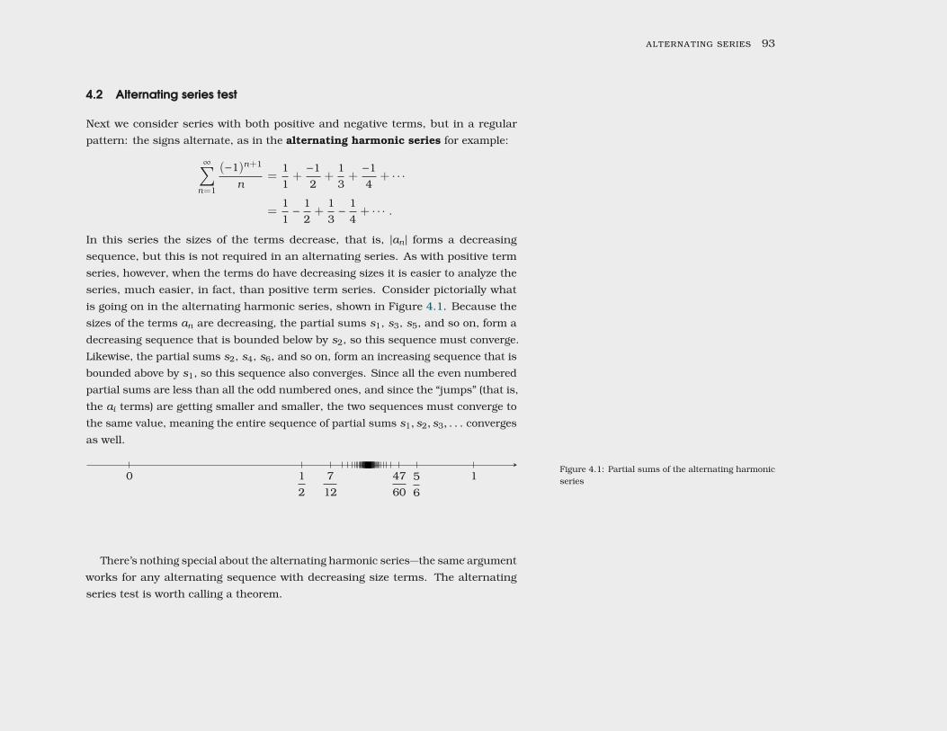
alternating series 93
4.2 Alternating series test
Next we consider series with both positive and negative terms, but in a regularpattern: the signs alternate, as in the alternating harmonic series for example:
∞∑n=1
(−1)n+1
n=
11+−12
+13+−14
+ · · ·
=11−
12+
13−
14+ · · · .
In this series the sizes of the terms decrease, that is, |an | forms a decreasingsequence, but this is not required in an alternating series. As with positive termseries, however, when the terms do have decreasing sizes it is easier to analyze theseries, much easier, in fact, than positive term series. Consider pictorially whatis going on in the alternating harmonic series, shown in Figure 4.1. Because thesizes of the terms an are decreasing, the partial sums s1, s3, s5, and so on, form adecreasing sequence that is bounded below by s2, so this sequence must converge.Likewise, the partial sums s2, s4, s6, and so on, form an increasing sequence that isbounded above by s1, so this sequence also converges. Since all the even numberedpartial sums are less than all the odd numbered ones, and since the “jumps” (that is,the ai terms) are getting smaller and smaller, the two sequences must converge tothe same value, meaning the entire sequence of partial sums s1, s2, s3, . . . convergesas well.
0 112
56
712
4760
Figure 4.1: Partial sums of the alternating harmonicseries
There’s nothing special about the alternating harmonic series—the same argumentworks for any alternating sequence with decreasing size terms. The alternatingseries test is worth calling a theorem.
94 sequences and series
Theorem 4.2.1 Suppose that (an) is a decreasing sequence of positive num-
bers and limn→∞
an = 0. Then the alternating series∞∑n=1
(−1)n+1an converges.
We have considered alternating series with first index1, and in which the first term is positive, but a littlethought shows this is not crucial. The same test
applies to any similar series, such as∞∑n=0
(−1)nan ,
∞∑n=1
(−1)nan ,∞∑
n=17(−1)nan , etc.
Proof The odd numbered partial sums, s1, s3, s5, and so on, form a de-
creasing sequence, because s2k+3 = s2k+1 − a2k+2 + a2k+3 ≤ s2k+1, since
a2k+2 ≥ a2k+3. This sequence is bounded below by s2, so it must converge,
say limk→∞
s2k+1 = L. Likewise, the partial sums s2, s4, s6, and so on, form
an increasing sequence that is bounded above by s1, so this sequence also
converges, say limk→∞
s2k = M . Since limn→∞
an = 0 and s2k+1 = s2k + a2k+1,
L = limk→∞
s2k+1 = limk→∞
(s2k + a2k+1) = limk→∞
s2k + limk→∞
a2k+1 = M + 0 = M ,
so L = M , the two sequences of partial sums converge to the same limit, and
this means the entire sequence of partial sums also converges to L.
We have shown more than convergence: if we are careful about thinking aboutthe previous argument, we can find error bounds. Let’s see how. Suppose that
L =∞∑n=1
(−1)n+1an
and that we approximate L by a finite part of this sum, say
L ≈N∑n=1
(−1)n+1an .
Because the terms are decreasing in size, we know that the true value of L must bebetween this approximation and the next one, that is, between
N∑n=1
(−1)n+1an andN+1∑n=1
(−1)n+1an .
Depending on whether N is odd or even, the second will be larger or smaller thanthe first. This is important enough that it deserves to be highlighted as a theorem.
alternating series 95
Theorem 4.2.2 Suppose that {an}∞n=1 is a decreasing sequence of positive
numbers and limn→∞
an = 0. By Theorem 4.2.1, we then know that∞∑n=1
(−1)n+1an
converges to some value, say L. Moreover, L is between
N∑n=1
(−1)n+1an andN+1∑n=1
(−1)n+1an .
Example 4.2.3 Approximate the alternating harmonic series to one decimalplace.
Solution We need to go roughly to the point at which the next term to beadded or subtracted is 1/10. Adding up the first nine and the first ten termswe get approximately 0.746 and 0.646. These are 1/10 apart, but it is notclear how the correct value would be rounded. It turns out that we are able tosettle the question by computing the sums of the first eleven and twelve terms,which give 0.737 and 0.653, so correct to one place the value is 0.7.
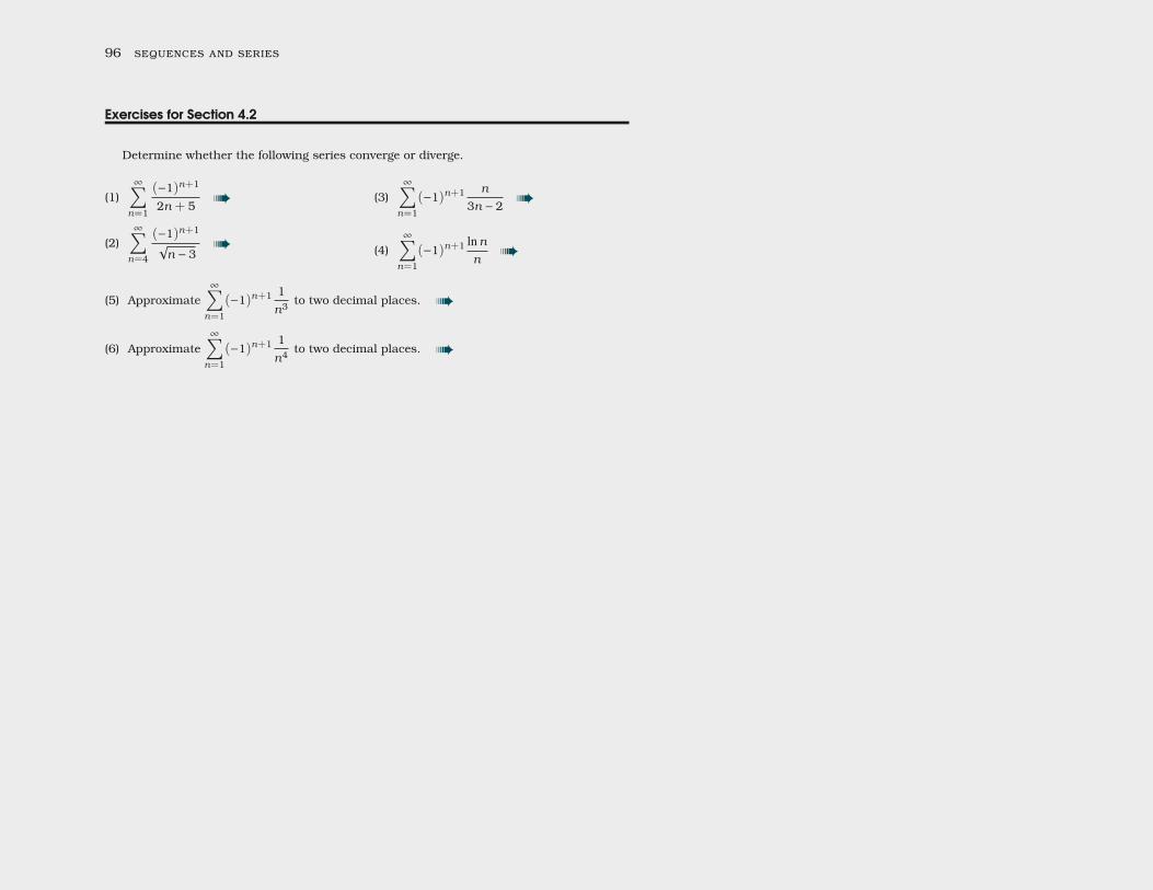
96 sequences and series
Exercises for Section 4.2
Determine whether the following series converge or diverge.
(1)∞∑n=1
(−1)n+1
2n + 5 à
(2)∞∑n=4
(−1)n+1√n − 3 à
(3)∞∑n=1
(−1)n+1 n
3n − 2 à
(4)∞∑n=1
(−1)n+1 lnnn à
(5) Approximate∞∑n=1
(−1)n+1 1n3 to two decimal places. à
(6) Approximate∞∑n=1
(−1)n+1 1n4 to two decimal places. à

5 Another comparison test
We’ve covered a ton of material thus far in this course; there is one more comparisontest that comes in quite handy—the Limit Comparison Test—which we will meet inSection 5.2. The purpose of this chapter, however, runs deeper than “just” anothercomparison test.
The emphasis on series has been almost entirely on the question of their conver-gence; we have not paid much heed to the value of the series, but we’ve developeda lot of techniques to analyze their convergence. The question is always “Does itconverge?” and the answer is “yes, it converges!” or “no, it does not converge.”Considering how qualitative our answer is, we might hope that there are equallyqualitative methods for analyzing series. If convergence is just a yes-or-no mat-ter, one might hope that the methods for analyzing series are equally loose andqualitative.
But that hasn’t been our experience. Convergence is a tricky business, requiringprecision and careful analysis. There have been hints, though, that things are easierthan they seem: the comparison test is perhaps the best example of that. In yourpast mathematical life, you’ve probably been given “expressions” or “equations” towhich you apply various rules in order to derive an answer. With the comparisontest, the situation is less about rules, and more about creatively ignoring parts ofthe expression in order to find a useful bound. More than being rule-based, testingconvergence via the comparison test requires some guesswork, and a willingness toignore the parts of the expression that don’t matter, in order to get at the part thatdoes.
Let me be more precise. Suppose we wanted to analyze the convergence of a
98 sequences and series
series such as∞∑
n=52
n4 − 3n + 52n5 + 5n3 − n2
This is a complicated series, but the given expression is the ratio between a fifthdegree polynomial and a fourth degree polynomial, so this series “is more or less”the same as the series
∞∑n=52
n4
n5 =∞∑
n=52
1n
which is the harmonic series, and diverges! This is how we’d like to think, but weneed to justify the concept of “is more or less.” This is what Section 5.2 will teachus to do.
5.1 Convergence depends on the tail
The harmonic series diverges, but so does the series
∞∑n=100
1n=
1100
+1
101+
1102
+1
103+ · · ·
Convergence doesn’t depend on the beginning of the series; whether or not I includethe first 99 terms
11+
12+
13+ · · ·+
197
+198
+199
does affect whether or the sum of all the terms diverges. In short, convergencedepends not on how a series begins, but on how a series ends. The end of a seriesis sometimes called the tail of the series.
Definition Let N > 1 be an integer, and consider a series∞∑n=1
an. The series
we get by removing the first N − 1 terms, namely
∞∑n=N
an
another comparison test 99
is called a tail of the given series.
Here is the theorem that describes how tails relate to convergence.
Theorem 5.1.1 Let N > 1 be an integer. The series∞∑n=1
an converges if and
only if∞∑n=N
an converges.
This could be shortened to “The series converges iff a tail of the series converges,” oreven just to the slogan that convergence depends on the tail.
Proof Suppose∞∑n=1
an converges to L, meaning
limM→∞
M∑n=1
an = L.
In that case, applying limit laws reveals
limM→∞
M∑n=N
an = limM→∞
M∑n=1
an
−N−1∑n=1
an
= limM→∞
M∑n=1
an
− limM→∞
N−1∑n=1
an
= lim
M→∞
M∑n=1
an
−N−1∑n=1
an
= L −
N−1∑n=1
an
,
100 sequences and series
which means the seriesM∑n=N
an converges.
The other direction is left to you, the reader.
Example 5.1.2 Does the series∞∑
n=153
1n2 converge?
Solution Yes! This series is a tail of the convergent p-series∞∑n=1
1n2 ; in this
case, p = 2.
You might recall Example 3.1.1, which we’ll redo here.
Example 5.1.3 Show that∞∑n=0
n5
5nconverges by using the comparison test and
Theorem 5.1.1.
Solution The given series converges iff∞∑
n=23
n5
5nby Theorem 5.1.1. But when-
ever n ≥ 23, we haven5
5n≤
2n
5n=
(25
)nThe series
∞∑n=23
(25
)nconverges, since it is a geometric series with common
ratio 2/5, so by comparison, the smaller series∞∑
n=23
n5
5nalso converges.
In light of Theorem 5.1.1, many textbooks will choose to write
∑n
an
another comparison test 101
instead of∞∑n=1
an when discussing convergence. Whether or not the series converges
doesn’t depend on the initial index, so if we want to state theorems about conver-gence, we can avoid potentially distracting details by simply not speaking aboutwhere the series begins.
5.2 Limit comparison test
This test is usually called the limit comparison test,
Theorem 5.2.1 Suppose an ≥ 0 and bn ≥ 0. Then if
limn→∞
anbn
= L > 0,
the series∞∑n=1
an converges if and only if∞∑n=1
bn converges.
The idea is that this is basically a comparison test, but instead of asking forsomething on the nose, like 0 ≤ an ≤ bn, I am instead asking only that an and bnbe similar in size.
5.2.1 Proof of the Limit Comparison Test
Assuming limn→∞
anbn
= L > 0, then we may also conclude that limn→∞
bnan
= 1/L > 0.
Theorem 5.2.2 Suppose an ≥ 0 and bn ≥ 0. Then if
limn→∞
anbn
= L > 0,
the series∞∑n=1
an converges if and only if∞∑n=1
bn converges.
102 sequences and series
5.2.2 How to apply the Limit Comparison Test
Example 5.2.3 Does the series
∞∑n=52
n4 − 3n + 52n5 + 5n3 − n2
converges or diverge?
Solution We will invoke the Limit Comparison Test, that is, Theorem 5.2.2.Set
an =n4 − 3n + 5
2n5 + 5n3 − n2 and bn =1n
,
so in this case,
limn→∞
anbn
= limn→∞
n4 − 3n + 52n5 + 5n3 − n2 ·
n
1
= limn→∞
n5 − 3n2 + 5n2n5 + 5n3 − n2
= limn→∞
n5 − 3n2 + 5n2n5 + 5n3 − n2 ·
1/n5
1/n5
= limn→∞
1 − 3n3 + 5
n4
2 + 5n2 −
1n3
=limn→∞
(1 − 3
n3 + 5n4
)limn→∞
(2 + 5
n2 −1n3
)=
12> 0,
and so∞∑
n=52
an and∞∑
n=52
bn share the same fate. But∞∑
n=52
bn diverges, and so
too does∞∑
n=52
an.
Of course, we could have just used a direct comparison test; the big benefit here isthat it is relatively painless to compute the limit, but it requires significant creativity
another comparison test 103
to set up a direct comparison test. Think back, for instance, to Example 3.1.1.

6 Power series
6.1 Definitions
At first, we studied the geometric series
∞∑n=0
(12
)n,
but then we replaced12
with a variable, so we were able to analyze all geometricseries simultaneously. In the end, we discovered that
∞∑n=0
kxn =k
1 − xif |x | < 1,
and that the series diverges when |x | ≥ 1. At the time, we thought of x as an You may recall that we used r instead of x; I think rwas a good choice back then, since r evokes “ratio”and stood for the common ratio between the termsin a geometric series. Now we use x, which I thinkis a good choice now. Why the change? To me, xsuggests “independent variable of a function” muchmore generally than just a parameter in a geometricseries, and we will be thinking very broadly abouthow quite general functions can be represented asa power series. One may regard power series as anatural generalization of polynomials, and you mayalready be comfortable thinking of x as the variablein a polynomial.
unspecified constant, but we could just as well think of it as a variable. A numberwhich depends on another number is just a function, so we may write
f (x) =∞∑n=0
kxn
and then observe that it is also the case that f (x) = k/(1 − x), as long as |x | < 1.While k/(1 − x) is a reasonably easy function to deal with, the more complicated∑
kxn does have its attractions: it appears to be an infinite version of one of thesimplest sorts of functions—a polynomial. Do other functions have representationsas series? Is there an advantage to viewing them in this way?
106 sequences and series
Usually the coefficients aren’t all the same in a polynomial; the geometric seriesis somewhat unusual in that all the coefficients of the powers of x are the same,namely k. We will need to allow more general coefficients if we are to get anythingother than the geometric series.
Definition Let (an) be a sequence of real numbers starting with a0. Then thepower series associated to (an) is
∞∑n=0
an xn .
Sometimes people are confused when considering, say,
∞∑n=0
(sin x) · xn .
Despite appearances, we will not be regarding such series as “power series.” Since(an) is a sequence of real numbers, the coefficients an cannot depend on x.
6.2 Convergence of power seriesIn Example 6.2.1, note that we are no longer con-sidering convergence of a single series; instead, byregarding x as a parameter, we are considering con-vergence for a whole family of series—namely all
those of the form∞∑n=1
xn/n. It often happens in
mathematics that it is wiser to study a family ofobjects simultaneously than to study a single objectin isolation.
Example 6.2.1 Consider the power series
f (x) =∞∑n=1
xn
n.
For which x does this converge?
Another way to think of this question is this: we are being asked to determinethe domain of f .
Solution We can investigate the convergence of this series using the ratio test.The difficulty now is that, instead of a single limit, we must now compute alimit than involves a variable x which is not the variable with respect to whichwe are taking a limit.
Another issue is that x may be negative, so we will actually check absolute
power series 107
convergence; in other words, we are actually considering
f (x) =∞∑n=1
∣∣∣∣∣xnn∣∣∣∣∣ .
Bravely,
L = limn→∞
|x |n+1
n+1|x |n
n
= limn→∞
|x |n+1
n + 1·
1|x |n
n
= limn→∞
|x |n+1
n + 1·n
|x |n
= limn→∞
|x |n+1 · n
(n + 1) · |x |n
= limn→∞
|x |n
n + 1= |x | · lim
n→∞
n
n + 1= |x |.
So when L = |x | < 1, the ratio test says that the series converges absolutely.When |x | > 1, the series does not converge absolutely—in fact, when |x | > 1, wehave that
limn→∞
xn
n, 0
and so the series diverges.So when |x | < 1 the series converges and when |x | > 1 it diverges, which
leaves only two values in doubt. When x = 1, the series is the harmonic seriesand diverges; when x = −1, it is the alternating harmonic series (rather, thenegative of the “usual” alternating harmonic series) and converges.
In other words, we may regard f as a function with domain [−1, 1).
We analyzed this power series by invoking the ratio test, but that was no accident.We will see that the ratio test applied to a power series will always have the same niceform. Feeling confident from our display of bravery before the preceding example,
108 sequences and series
let’s attack the general case of a power series
f (x) =∞∑n=0
an xn .
When does this series converge absolutely? Applying the ratio test again, we find
L = limn→∞
|an+1| · |x |n+1
|an | · |x |n
= limn→∞
|x | ·|an+1|
|an |
= |x | · limn→∞
|an+1|
|an |.
So the series converges absolutely whenever L < 1, but in this case, L depends in arather uncomplicated way on |x |. The whole story is controlled by a limit that does
not depend on x, namely
1/R = limn→∞
|an+1|
|an |,
which you see I have presciently related to a hitherto unmentioned variable, R. Sothe series converges absolutely whenever |x |/R < 1, meaning the series convergesabsolutely whenever |x | < R. When |x | > R, the series diverges1. 1 This is a consequent of the ratio test, but perhaps
we haven’t emphasized it enough; if L > 1 in theratio test, then the limit of the terms is not zero, sonot only does the series not converge absolutely—theoriginal series diverges, too, by the limit test.
Once again, only the two values x = ±R require further investigation. In anycase, if we begin with a sequence (an) for which
1/R = limn→∞
|an+1|
|an |,
the associated power series∞∑n=0
anxn will converge for values of x in the interval
(−R,R), and it may even converge (or not, depending on the specific situation) atx = R or at x = −R, so sometimes the interval on which the series makes sense willbe [−R,R) or (−R,R] or even [−R,R].
power series 109
Definition The set of values of x for which the series∞∑n=0
an xn converges is
the interval of convergence.
As a consequence of the above discussion, the interval of convergence of a powerseries always have a nice form.
Theorem 6.2.2 For a power series, the interval of convergence is, in fact, aninterval. It has the form (−R,R) or [−R,R) or (−R,R] or [−R,R]. In short, it iscentered around 0.
Because the interval of convergence is, indeed, centered around 0, and becausewe often don’t care about what happens at the endpoint, it is often convenient tojust describe R.
Definition In the interval of convergence of a power series, the value R iscalled the radius of convergence of the series.
Two special cases deserve mention. If
limn→∞
|an+1|
|an |= 0,
then we might say “R = ∞” since no matter what x is, the product
|x | limn→∞
|an+1|
|an |= 0,
and therefore for all values of x, the power series∞∑n=0
an xn converges. So the radius
of convergence, R, is infinite.The opposite may happen as well. It may happen that
limn→∞
|an+1|
|an |= ∞,
110 sequences and series
in which case the only way that
|x | limn→∞
|an+1|
|an |< 1
is when |x | = 0. The interval of convergence is just the single point {0}. And in thiscase, we say R = 0.
Warning People often confuse “radius of convergence” with “interval of con-vergence.” For starters, the radius of convergence is a single number, whilethe interval of convergence is, well, an interval (though it was defined as just aset—the fact that the set where the series converges is an interval was a theoremand was certainly not obvious—perhaps the first of many lovely surprises withpower series).
There is another difference between the radius of convergence and theinterval of convergence; it is not simply that they are the same informationin different packages. The radius of convergence cannot distinguish between,say, (−R,R) versus [−R,R]. The interval of convergence contains the extrainformation about what is happening at the endpoints. So a homework questionwhich asks you to find the radius R is much easier than a homework questionasking you to find the interval.
6.3 Power series centered elsewhere
If we are speaking of the “radius” of convergence, you might wonder about the “center”of convergence. Thus far, our intervals of convergence have been centered aroundthe origin, but by changing the series, we can move the interval of convergence.Let’s see how.
Consider once again the geometric series,
f (x) =∞∑n=0
xn =1
1 − xfor x ∈ (−1, 1).
Whatever benefits there might be in using the series form of this function are only
power series 111
available to us when x is between −1 and 1. We can address this shortcoming bymodifying the power series slightly.
Example 6.3.1 Find a series representation for1
1 − xvalid on the interval
(−5, 1).
Solution Consider that the series
∞∑n=0
(x + 2)n
3n=
∞∑n=0
(x + 23
)n=
11 − x+2
3=
31 − x
,
because this is just a geometric series with x replaced by (x+2)/3. Multiplyingboth sides by 1/3 gives
∞∑n=0
(x + 2)n
3n+1 =1
1 − x,
the same function as before. For what values of x does this series converge?Since it is a geometric series, we know that it converges when
|x + 2|/3 < 1
|x + 2| < 3
−3 < x + 2 < 3
−5 < x < 1.
So we have a series representation for 1/(1− x) that works on a larger intervalthan before, at the expense of a somewhat more complicated series. Theendpoints of the interval of convergence now are −5 and 1, but note that thosetwo endpoints can be described as −2 ± 3. We say that 3 is the radius ofconvergence, and we now say that the series is centered at −2.
Let’s capture this in a definition. It is worth contrasting Definition 18 with Defini-tion 15, our original description of power series. In
particular,∞∑n=0
an xn is a power series centered at
zero.
112 sequences and series
Definition Let (an) be a sequence of real numbers starting with a0. Then thepower series centered at c and associated to (an) is the series
∞∑n=0
an (x − c)n .
In Example 6.3.1, we formed a series that involved (x + 2)n, meaning that inthat case c = −2.
You are now in a position to try your hand at finding the radius of convergenceand sometimes even the interval of convergence for some power series. I encourageyou to cook up your own power series, and then see what you can say about theradius and interval of convergence.
power series 113
Exercises for Section 6.3
Find the radius and interval of convergence for each series. In exercises 3 and 4, do notattempt to determine whether the endpoints are in the interval of convergence.
(1)∞∑n=0
nxn à
(2)∞∑n=0
xn
n! à
(3)∞∑n=1
n!nnxn à
(4)∞∑n=1
n!nn
(x − 2)n à
(5)∞∑n=1
(n!)2
nn(x − 2)n à
(6)∞∑n=1
(x + 5)n
n(n + 1) à
(7) Find a power series with radius of convergence 0. à
114 sequences and series
6.4 Calculus with power series
Now we know that some functions can be expressed as power series, which looklike infinite polynomials. Since calculus, that is, computation of derivatives andantiderivatives, is easy for polynomials, the obvious question is whether the same istrue for infinite series. The answer is yes!
Theorem 6.4.1 Suppose the power series f (x) =∞∑n=0
an(x − c)n has radius
of convergence R. Then
f ′(x) =∞∑n=1
nan(x − c)n−1,
∫f (x) dx = C+
∞∑n=0
ann + 1
(x − c)n+1,
for values of x in the interval (c − R, c + R). The two new series have radius ofconvergence R, just like the original series.
Example 6.4.2 Find an alternating series for log(32
). Approximate this value
to two decimal places.
Solution Begin with the geometric series, namely
11 − x
=∞∑n=0
xn .

power series 115
Then integrate term-by-term to find∫1
1 − xdx = − log |1 − x | =
∞∑n=0
1n + 1
xn+1
log |1 − x | =∞∑n=0−
1n + 1
xn+1
for real numbers x such that |x | < 1. To compute log(3/2), we should choosex = −1/2. In that case,
log(3/2) = log(1 − −1/2)
=∞∑n=0
(−1)n1
n + 11
2n+1
and so
log(3/2) ≈12−
18+
124−
164
+1
160−
1384
+1
896=
9092240
≈ 0.406.
Because this is an alternating series with decreasing terms, we know that thetrue value is between 909/2240 and 909/2240 − 1/2048 = 29053/71680 ≈.4053, so log(3/2) is, to two decimal places, 0.41.
Example 6.4.3 What about log(9/4)? Find an approximate value for it.
Solution Since 9/4 is larger than 2 we cannot use the series directly, but
log(9/4) = log((3/2)2) = 2 log(3/2) ≈ 0.82,
so in fact we get a lot more from this one calculation than first meets the eye.To estimate the true value accurately we actually need to be a bit more careful.
When we multiply by two we know that the true value is between 0.8106and 0.812, and so, rounded to two decimal places, the true value is 0.81.
116 sequences and series
Exercises for Section 6.4
(1) Find a series representation for log 2. à(2) Find a power series representation for 1/(1 − x)2. à(3) Find a power series representation for 2/(1 − x)3. à(4) Find a power series representation for 1/(1 − x)3. What is the radius of convergence?
à
(5) Find a power series representation for∫
log(1 − x) dx. à
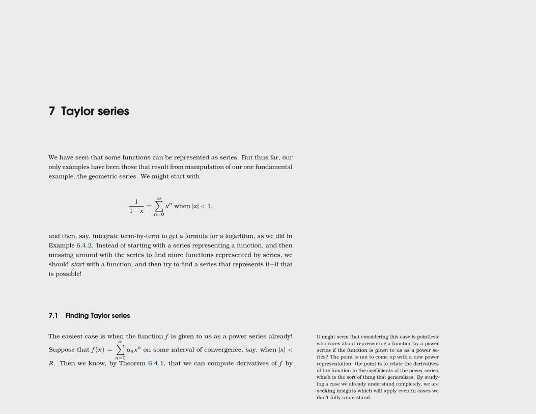
7 Taylor series
We have seen that some functions can be represented as series. But thus far, ouronly examples have been those that result from manipulation of our one fundamentalexample, the geometric series. We might start with
11 − x
=∞∑n=0
xn when |x | < 1,
and then, say, integrate term-by-term to get a formula for a logarithm, as we did inExample 6.4.2. Instead of starting with a series representing a function, and thenmessing around with the series to find more functions represented by series, weshould start with a function, and then try to find a series that represents it—if thatis possible!
7.1 Finding Taylor series
The easiest case is when the function f is given to us as a power series already! It might seem that considering this case is pointless:who cares about representing a function by a powerseries if the function is given to us as a power se-ries? The point is not to come up with a new powerrepresentation: the point is to relate the derivativesof the function to the coefficients of the power series,which is the sort of thing that generalizes. By study-ing a case we already understand completely, we areseeking insights which will apply even in cases wedon’t fully understand.
Suppose that f (x) =∞∑n=0
anxn on some interval of convergence, say, when |x | <
R. Then we know, by Theorem 6.4.1, that we can compute derivatives of f by

118 sequences and series
differentiating the series term-by-term. Let’s look at the first few derivatives.
f ′(x) =∞∑n=1
nanxn−1 = a1 + 2a2x + 3a3x
2 + 4a4x3 + · · ·
f ′′(x) =∞∑n=2
n(n − 1)anxn−2 = 2a2 + 3 · 2a3x + 4 · 3a4x2 + · · ·
f ′′′(x) =∞∑n=3
n(n − 1)(n − 2)anxn−3 = 3 · 2a3 + 4 · 3 · 2a4x + · · ·
By examining these derivatives, we can discern the general pattern. The kth
derivative must be Recall that, for a function f , we write its kth deriva-tive by writing f (k). So the kth derivative evaluatedat x is written f (k)(x).
f (k)(x) =∞∑n=k
n(n − 1)(n − 2) · · · (n − k + 1)anxn−k
= k(k − 1)(k − 2) · · · (2)(1)ak + (k + 1)(k) · · · (2)ak+1x +
+ (k + 2)(k + 1) · · · (3)ak+2x2 + · · · ,
but we can write this more easily by using factorials, namely
f (k)(x) =∞∑n=k
n!(n − k)!
anxn−k = k!ak + (k + 1)!ak+1x +
(k + 2)!2!
ak+2x2 + · · · .
Now, substituting x = 0 yields
f (k)(0) = k!ak +∞∑
n=k+1
n!(n − k)!
an0n−k = k!ak ,
and solving for ak gives
ak =f (k)(0)k!
.
So if a function f can be represented by a series, we know just what series it is! Weknow the series because we know the derivatives of f . Note that ak = f (k)(0)/k! makes sense even when
k = 0, since in that special case, we have a0 =f (0)(0)/0! = f (0) because the zeroth derivative of fis f itself, and 0! = 1.
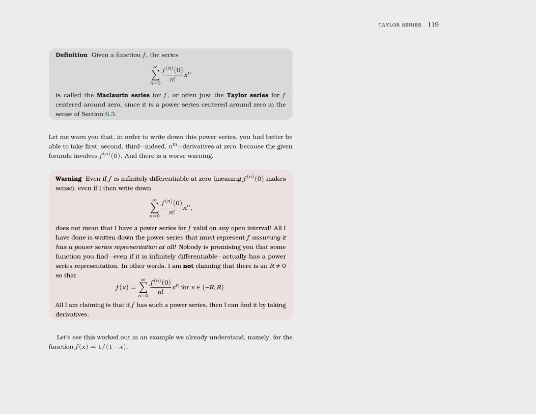
taylor series 119
Definition Given a function f , the series
∞∑n=0
f (n)(0)n!
xn
is called the Maclaurin series for f , or often just the Taylor series for fcentered around zero, since it is a power series centered around zero in thesense of Section 6.3.
Let me warn you that, in order to write down this power series, you had better beable to take first, second, third—indeed, nth—derivatives at zero, because the givenformula involves f (n)(0). And there is a worse warning.
Warning Even if f is infinitely differentiable at zero (meaning f (n)(0) makessense), even if I then write down
∞∑n=0
f (n)(0)n!
xn ,
does not mean that I have a power series for f valid on any open interval! All Ihave done is written down the power series that must represent f assuming it
has a power series representation at all! Nobody is promising you that somefunction you find—even if it is infinitely differentiable—actually has a powerseries representation. In other words, I am not claiming that there is an R , 0so that
f (x) =∞∑n=0
f (n)(0)n!
xn for x ∈ (−R,R).
All I am claiming is that if f has such a power series, then I can find it by takingderivatives.
Let’s see this worked out in an example we already understand, namely, for thefunction f (x) = 1/(1 − x).
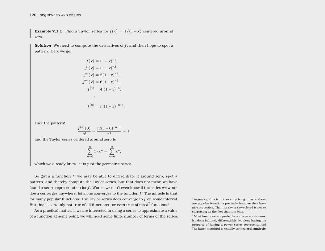
120 sequences and series
Example 7.1.1 Find a Taylor series for f (x) = 1/(1 − x) centered aroundzero.
Solution We need to compute the derivatives of f , and then hope to spot apattern. Here we go:
f (x) = (1 − x)−1,
f ′(x) = (1 − x)−2,
f ′′(x) = 2(1 − x)−3,
f ′′′(x) = 6(1 − x)−4,
f (4) = 4!(1 − x)−5,
...
f (n) = n!(1 − x)−n−1.
I see the pattern!f (n)(0)n!
=n!(1 − 0)−n−1
n!= 1,
and the Taylor series centered around zero is
∞∑n=0
1 · xn =∞∑n=0
xn ,
which we already knew—it is just the geometric series.
So given a function f , we may be able to differentiate it around zero, spot apattern, and thereby compute the Taylor series, but that does not mean we havefound a series representation for f . Worse, we don’t even know if the series we wrotedown converges anywhere, let alone converges to the function f ! The miracle is thatfor many popular functions1 the Taylor series does converge to f on some interval. 1 Arguably, this is not so surprising: maybe these
are popular functions precisely because they havenice properties. That the sky is sky-colored is not sosurprising as the fact that it is blue.
But this is certainly not true of all functions—or even true of most2 functions!
2 Most functions are probably not even continuous,let alone infinitely differentiable, let alone having theproperty of having a power series representation!The latter mouthful is usually termed real analytic.
As a practical matter, if we are interested in using a series to approximate a valueof a function at some point, we will need some finite number of terms of the series.
taylor series 121
Even for functions with terrible looking derivatives, we can compute the initial termsusing computer software like Sage. If we want to know the whole series—that is, thenth term in the series for an arbitrary n—then we need a function whose derivativesfall into a pattern that we can discern. A few of the most popular functions havenice patterns. Let’s see some now!
Example 7.1.2 Find a Taylor series for sin x.
Solution The derivatives are quite easy, namely
f ′(x) = cos x ,
f ′′(x) = − sin x ,
f ′′′(x) = − cos x ,
f (4)(x) = sin x ,
and then the pattern repeats. We want to know the derivatives at zero, sothose are
f ′(0) = cos 0 = 1
f ′′(0) = − sin 0 = 0
f ′′′(0) = − cos 0 = −1,
f (4)(0) = sin 0 = 0,
and then the pattern repeats, namely it goes—starting from the zeroth derivative—like this:
0, 1, 0, −1, 0, 1, 0, −1, 0, . . . .
And so, the Taylor series is
x −x3
3!+x5
5!− · · · =
∞∑n=0
(−1)nx2n+1
(2n + 1)!.
Sometimes people are confused by the fact that the exponent in this powerseries is 2n + 1 instead of just n. It turns out that setting it up this way,with x2n+1, nicely manages to kill all the terms xeven number which have a zero
122 sequences and series
coefficient, since differentiating f an even number of times results in ± sin x,which is zero when x = 0.
But there is more to be anxious about. Before worrying whether this seriesconverges to sin x, we should ask the prior question: does this series convergeanywhere? Let’s determine the radius of convergence by using the ratio test,which asks us to consider
L = limn→∞
|x |2n+3
(2n + 3)!(2n + 1)!|x |2n+1
= limn→∞
|x |2
(2n + 3)(2n + 2)= 0,
and so the series converges regardless of what x is. It will turn out later, byapplying Theorem 7.2.1, that this series does converge to sin x.
Sometimes the formula for the nth derivative of a function f is difficult to discover,but a combination of a known Taylor series and some algebraic manipulation leadseasily to the Taylor series for f .
Example 7.1.3 Find the Taylor series for f (x) = x sin(−x) centered at zero.
Solution To get from sin x to x sin(−x) we substitute −x for x and then multiplyby x. Let’s do the same thing to the series for sin x, namely
x∞∑n=0
(−1)n(−x)2n+1
(2n + 1)!= x
∞∑n=0
(−1)n(−1)2n+1 x2n+1
(2n + 1)!
=∞∑n=0
(−1)n+1 x2n+2
(2n + 1)!.
taylor series 123
Of course, we could have differentiated f (x), which would have yielded
f ′(x) = −x cos (−x) + sin (−x) = 0,
f ′′(x) = −x sin (−x) − 2 cos (−x) = −2,
f ′′′(x) = x cos (−x) − 3 sin (−x) = 0,
f (4)(x) = x sin (−x) + 4 cos (−x) = 4,
but maybe it would have been harder to pick up on the pattern that way.
As we have seen in Section 6.3, a general power series can be centered at a pointother than zero, and the method that produces the Taylor series can also producesuch series.
Definition Given a function f , the series
∞∑n=0
f (n)(c)
n!(x − c)n
is called the Taylor series for f centered around c.
Let’s see an example, reminiscent of Example 6.3.1 but attacked with a differentmethod.
Example 7.1.4 Find a Taylor series centered at −2 for 1/(1 − x).
Solution If the series is∞∑n=0
an(x + 2)n then looking at the kth derivative:
k!(1 − x)−k−1 =∞∑n=k
n!(n − k)!
an(x + 2)n−k
124 sequences and series
and substituting x = −2 we get k!3−k−1 = k!ak and ak = 3−k−1 = 1/3k+1, sothe series is
∞∑n=0
(x + 2)n
3n+1 .
taylor series 125
Exercises for Section 7.1
For each function, find the Taylor series centered at c, and the radius of convergence. Donot worry about whether or not the series converges to the given function—that will be ourconcern in Section 7.2.
(1) cos x around c = 0, à(2) ex around c = 0, à(3) 1/x around c = 5 à(4) log x around c = 1 à(5) log x around c = 2 à(6) 1/x2 around c = 1 à(7) 1/
√1 − x around c = 0 à
(8) Find the first four terms of the Taylor series for tan x centered at zero. By “first four terms”I mean up to and including the x3 term. à
(9) Use a combination of Taylor series and algebraic manipulation to find a series centeredat zero for x cos(x2). à
(10) Use a combination of Taylor series and algebraic manipulation to find a series centeredat zero for xe−x . à
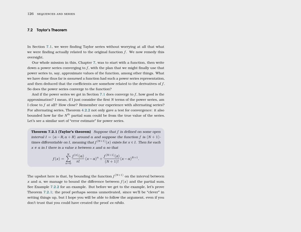
126 sequences and series
7.2 Taylor’s Theorem
In Section 7.1, we were finding Taylor series without worrying at all that whatwe were finding actually related to the original function f . We now remedy thisoversight.
Our whole mission in this, Chapter 7, was to start with a function, then writedown a power series converging to f , with the plan that we might finally use thatpower series to, say, approximate values of the function, among other things. Whatwe have done thus far is assumed a function had such a power series representation,and then deduced that the coefficients are somehow related to the derivatives of f .So does the power series converge to the function?
And if the power series we got in Section 7.1 does converge to f , how good is theapproximation? I mean, if I just consider the first N terms of the power series, amI close to f at all? How close? Remember our experience with alternating series?For alternating series, Theorem 4.2.2 not only gave a test for convergence: it alsobounded how far the N th partial sum could be from the true value of the series.Let’s see a similar sort of “error estimate” for power series.
Theorem 7.2.1 (Taylor’s theorem) Suppose that f is defined on some openinterval I = (a − R,a + R) around a and suppose the function f is (N + 1)-times differentiable on I, meaning that f (N+1)(x) exists for x ∈ I. Then for eachx , a in I there is a value z between x and a so that
f (x) =N∑n=0
f (n)(a)
n!(x − a)n +
f (N+1)(z)
(N + 1)!(x − a)N+1.
The upshot here is that, by bounding the function f (N+1) on the interval betweenx and a, we manage to bound the difference between f (x) and the partial sum.See Example 7.2.2 for an example. But before we get to the example, let’s proveTheorem 7.2.1; the proof perhaps seems unmotivated, since we’ll be “clever” insetting things up, but I hope you will be able to follow the argument, even if youdon’t trust that you could have created the proof ex nihilo.
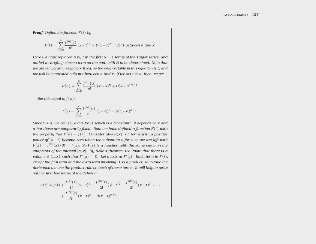
taylor series 127
Proof Define the function F (t) by
F (t) =N∑n=0
f (n)(t)
n!(x − t)n + B(x − t)N+1 for t between a and x.
Here we have replaced a by t in the first N + 1 terms of the Taylor series, and
added a carefully chosen term on the end, with B to be determined. Note that
we are temporarily keeping x fixed, so the only variable in this equation is t, and
we will be interested only in t between a and x. If we set t = a, then we get
F (a) =N∑n=0
f (n)(a)
n!(x − a)n + B(x − a)N+1.
Set this equal to f (x):
f (x) =N∑n=0
f (n)(a)
n!(x − a)n + B(x − a)N+1.
Since x , a, we can solve this for B, which is a “constant”—it depends on x and
a but those are temporarily fixed. Now we have defined a function F (t) with
the property that F (a) = f (x). Consider also F (x): all terms with a positive
power of (x − t) become zero when we substitute x for t, so we are left with
F (x) = f (0)(x)/0! = f (x). So F (t) is a function with the same value on the
endpoints of the interval [a, x ]. By Rolle’s theorem, we know that there is a
value z ∈ (a, x) such that F ′(z) = 0. Let’s look at F ′(t). Each term in F (t),
except the first term and the extra term involving B, is a product, so to take the
derivative we use the product rule on each of these terms. It will help to write
out the first few terms of the definition:
F (t) = f (t) +f (1)(t)
1!(x − t)1 +
f (2)(t)
2!(x − t)2 +
f (3)(t)
3!(x − t)3 + · · ·
+f (N)(t)
N !(x − t)N + B(x − t)N+1.
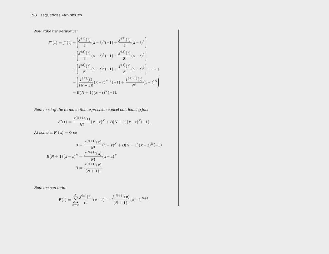
128 sequences and series
Now take the derivative:
F ′(t) = f ′(t) +
f (1)(t)1!(x − t)0(−1) +
f (2)(t)
1!(x − t)1
+
f (2)(t)1!(x − t)1(−1) +
f (3)(t)
2!(x − t)2
+
f (3)(t)2!(x − t)2(−1) +
f (4)(t)
3!(x − t)3
+ · · ·++
f (N)(t)(N − 1)!(x − t)N−1(−1) +
f (N+1)(t)
N !(x − t)N
+ B(N + 1)(x − t)N (−1).
Now most of the terms in this expression cancel out, leaving just
F ′(t) =f (N+1)(t)
N !(x − t)N + B(N + 1)(x − t)N (−1).
At some z, F ′(z) = 0 so
0 =f (N+1)(z)
N !(x − z)N + B(N + 1)(x − z)N (−1)
B(N + 1)(x − z)N =f (N+1)(z)
N !(x − z)N
B =f (N+1)(z)
(N + 1)!.
Now we can write
F (t) =N∑n=0
f (n)(t)
n!(x − t)n +
f (N+1)(z)
(N + 1)!(x − t)N+1.
taylor series 129
Recalling that F (a) = f (x) we get
f (x) =N∑n=0
f (n)(a)
n!(x − a)n +
f (N+1)(z)
(N + 1)!(x − a)N+1,
which is what we wanted to show.
It may not be immediately obvious that this is particularly useful, so let’s look atsome examples of Theorem 7.2.1 in action.
Example 7.2.2 Suppose x ∈ [−π/2, π/2]. Find a polynomial approximationfor sin x accurate to ±0.005.
Solution Note that if we can compute sin x for x ∈ [−π/2, π/2], then we cancompute sin x for all x. So what we are asking for here is actually quite general!Once we figure out how to calculate sin x for x ∈ [−π/2, π/2], we can shift anyother value of x into that interval, and thereby compute sin x.
Let’s get started. From Theorem 7.2.1, we have that
sin x =N∑n=0
f (n)(a)
n!(x −a)n+
f (N+1)(z)
(N + 1)!(x −a)N+1 for some z between a and x.
What can we say about the size of that “error” term? In other words, how bigcould
f (N+1)(z)
(N + 1)!(x − a)N+1
possibly be when z is between x and a? Every derivative of sin x is either ± sin xor ± cos x, so |f (N+1)(z)| ≤ 1. The factor (x − a)N+1 is a bit more difficult, sincex − a could be quite large. To simplify matters, let’s pick a = 0. We need topick N so that ∣∣∣∣∣∣ xN+1
(N + 1)!
∣∣∣∣∣∣ < 0.005.
Since we are only considering the case when x ∈ [−π/2, π/2], we have∣∣∣∣∣∣ xN+1
(N + 1)!
∣∣∣∣∣∣ < 2N+1
(N + 1)!.
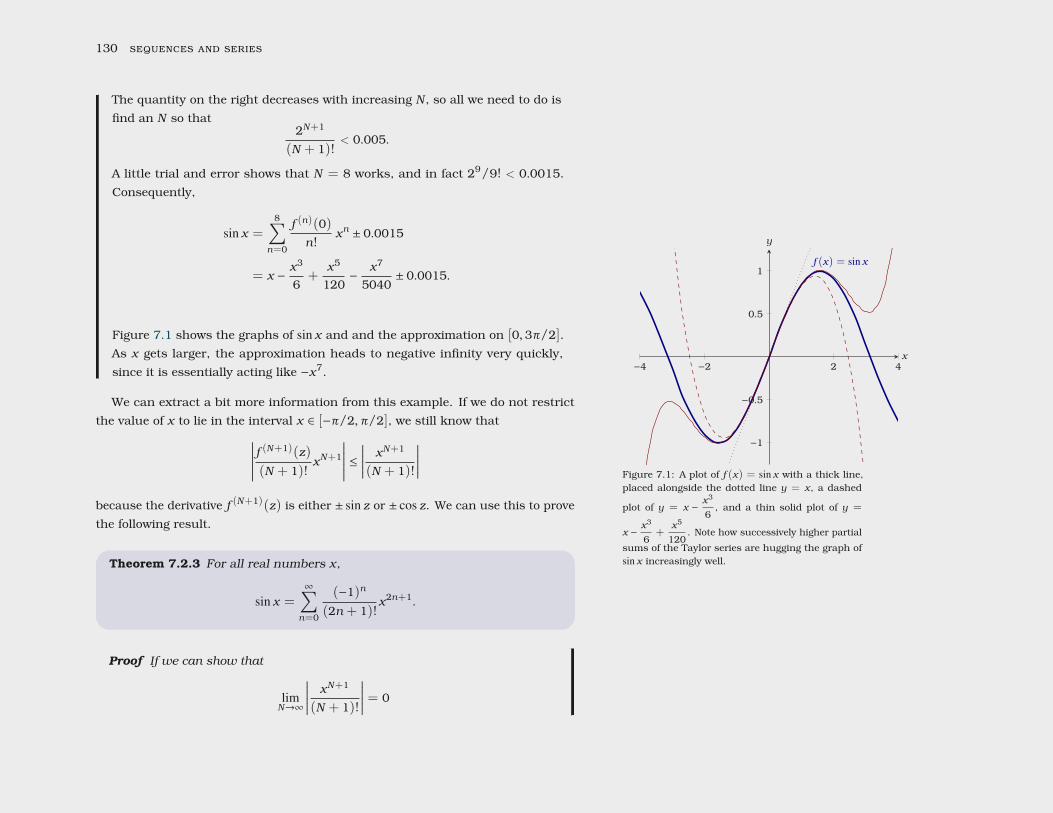
130 sequences and series
The quantity on the right decreases with increasing N , so all we need to do isfind an N so that
2N+1
(N + 1)!< 0.005.
A little trial and error shows that N = 8 works, and in fact 29/9! < 0.0015.Consequently,
sin x =8∑
n=0
f (n)(0)n!
xn ± 0.0015
= x −x3
6+
x5
120−
x7
5040± 0.0015.
Figure 7.1 shows the graphs of sin x and and the approximation on [0, 3π/2].As x gets larger, the approximation heads to negative infinity very quickly,since it is essentially acting like −x7. −4 −2 2 4
−1
−0.5
0.5
1f (x) = sin x
x
y
Figure 7.1: A plot of f (x) = sin x with a thick line,placed alongside the dotted line y = x, a dashed
plot of y = x −x3
6, and a thin solid plot of y =
x −x3
6+
x5
120. Note how successively higher partial
sums of the Taylor series are hugging the graph ofsin x increasingly well.
We can extract a bit more information from this example. If we do not restrictthe value of x to lie in the interval x ∈ [−π/2, π/2], we still know that∣∣∣∣∣∣∣ f (N+1)(z)
(N + 1)!xN+1
∣∣∣∣∣∣∣ ≤∣∣∣∣∣∣ xN+1
(N + 1)!
∣∣∣∣∣∣because the derivative f (N+1)(z) is either ± sin z or ± cos z. We can use this to provethe following result.
Theorem 7.2.3 For all real numbers x,
sin x =∞∑n=0
(−1)n
(2n + 1)!x2n+1.
Proof If we can show that
limN→∞
∣∣∣∣∣∣ xN+1
(N + 1)!
∣∣∣∣∣∣ = 0
taylor series 131
for each x, then we know that the error term∣∣∣∣∣∣∣ f (N+1)(z)
(N + 1)!xN+1
∣∣∣∣∣∣∣ ≤∣∣∣∣∣∣ xN+1
(N + 1)!
∣∣∣∣∣∣ ,is, in the limit, zero, and so we may conclude that
sin x =∞∑n=0
f (n)(0)n!
xn
=∞∑n=0
(−1)nx2n+1
(2n + 1)!.
In other words, we will conclude that the sine function is actually equal to its
Taylor series around zero for all x. But how can we prove that the limit is zero?
Suppose that N is larger than |x |, and let M be the largest integer less than |x |.
If M = 0, then xN+1 is small, and even smaller after dividing by (N + 1)!. On
the other hand, if M > 0, then just a bit more work is called for. We compute that
|xN+1|
(N + 1)!=
|x |
N + 1|x |
N
|x |
N − 1· · ·
|x |
M + 1|x |
M
|x |
M − 1· · ·|x |
2|x |
1
≤|x |
N + 1· 1 · 1 · · ·1 ·
|x |
M
|x |
M − 1· · ·|x |
2|x |
1
=|x |
N + 1|x |M
M !.
The quantity |x |M/M ! is a constant, so
limN→∞
|x |
N + 1|x |M
M != 0
and by squeezing via Theorem 1.7.2,
limN→∞
∣∣∣∣∣∣ xN+1
(N + 1)!
∣∣∣∣∣∣ = 0
as desired.
Essentially the same argument works for cos x, which yields the following.
132 sequences and series
Theorem 7.2.4 For all real numbers x,
cos x =∞∑n=0
(−1)n
(2n)!x2n .
And similarly, the function ex is real analytic, meaning that the Taylor seriesfor ex converges to ex .
Theorem 7.2.5 For all real numbers x,
ex =∞∑n=0
1n!xn .
Example 7.2.6 Find a polynomial approximation for ex near x = 2 accurateto ±0.005.
Solution From Taylor’s theorem:
ex =N∑n=0
e2
n!(x − 2)n +
ez
(N + 1)!(x − 2)N+1,
since f (n)(x) = ex for all n. We are interested in x near 2, and we need tocontrol the size of |(x − 2)N+1|, so we may as well specify that |x − 2| ≤ 1,meaning x ∈ [1, 3]. Also ∣∣∣∣∣∣ ez
(N + 1)!
∣∣∣∣∣∣ ≤ e3
(N + 1)!,
taylor series 133
so we need to find an N that makes e3/(N + 1)! ≤ 0.005. This time N = 6makes e3/(N + 1)! < 0.004, so the approximating polynomial is
ex = e2 + e2(x −2)+e2
2(x −2)2 +
e2
6(x −2)3 +
e2
24(x −2)4 +
e2
120(x −2)5 +
e2
720(x −2)6±0.004.
This presents an additional problem for approximation, since we also need toapproximate e2, and any approximation we use will increase the error, but wewill not pursue this complication.
Note well that in these examples we found polynomials of a certain accuracy onlyon a small interval, even though the series for sin x and ex converge for all x. Thisis usually how things work out. To get the same accuracy on a larger interval, whatcan you do? Use more terms!
134 sequences and series
Exercises for Section 7.2
(1) Find a polynomial approximation for cos x on [0, π], accurate to ±10−3 à(2) How many terms of the series for log x centered at 1 are required so that the guaranteed
error on [1/2, 3/2] is at most 10−3? What if the interval is instead [1, 3/2]? à(3) Find the first three nonzero terms in the Taylor series for tan x on [−π/4, π/4], and
compute the guaranteed error term as given by Taylor’s theorem. (You may want to useSage or a similar aid.) à
(4) Prove Theorem 7.2.4, that is, show that cos x is equal to its Taylor series for all x byshowing that the limit of the error term is zero as N approaches infinity. à
(5) Prove Theorem 7.2.5, that is, show that ex is equal to its Taylor series for all x by showingthat the limit of the error term is zero as N approaches infinity. à

Review
These problems require various techniques, and are in no particular order. Manyproblems may be done in more than one way.
I also encourage you to try your hand at crafting your own problems: mathematicsis more than answer-getting—it is also about problem-posing! Building your ownproblems will give you a strong sense of the limitations of the machinery we havebuilt in this book.
136 sequences and series
Exercises for Section 7.2
Determine whether the series converges.
(1)∞∑n=0
n
n2 + 4 à
(2)1
1 · 2+
13 · 4
+1
5 · 6+
17 · 8
+ · · · à
(3)∞∑n=0
n
(n2 + 4)2 à
(4)∞∑n=0
n!8n à
(5) 1 −34+
58−
712
+916
+ · · · à
(6)∞∑n=0
1√n2 + 4 à
(7)∞∑n=0
sin3(n)
n2 à
(8)∞∑n=0
n
en à
(9)∞∑n=0
n!1 · 3 · 5 · · · (2n − 1) à
(10)∞∑n=1
1n√n à
(11)1
2 · 3 · 4+
23 · 4 · 5
+3
4 · 5 · 6+
45 · 6 · 7
+ · · · à
(12)∞∑n=1
1 · 3 · 5 · · · (2n − 1)(2n)! à
(13)∞∑n=0
6n
n! à
(14)∞∑n=1
(−1)n−1√n à
taylor series 137
(15)∞∑n=1
2n3n−1
n! à
(16) 1 +52
22 +54
(2 · 4)2 +56
(2 · 4 · 6)2 +58
(2 · 4 · 6 · 8)2 + · · · à
(17)∞∑n=1
sin(1/n) à
Find the interval and radius of convergence; you need not check the endpoints of the intervals.
(18)∞∑n=0
2n
n!xn à
(19)∞∑n=0
xn
1 + 3n à
(20)∞∑n=1
xn
n3n à
(21) x +12x3
3+
1 · 32 · 4
x5
5+
1 · 3 · 52 · 4 · 6
x7
7+ · · · à
(22)∞∑n=1
n!n2 x
n à
(23)∞∑n=1
(−1)n
n23nx2n à
(24)∞∑n=0
(x − 1)n
n! à
Find a series for each function, using the formula for Maclaurin series and algebraicmanipulation as appropriate.
(25) 2x à(26) ln(1 + x) à(27) ln
(1 + x
1 − x
)à
(28)√
1 + x à(29)
11 + x2 à
(30) arctan(x) à(31) Use the answer to the previous problem to discover a series for a well-known mathematical
constant. à


Epilogue (or. . . what happens to Harry?)
The worst part about reading a great3 novel is that last page. The book gets thinner 3 Or even a bad novel.
and thinner, and then, poof! Not just the characters, but the whole world that theauthor has crafted for them is gone! And how frequently I want to stay in that worldjust a bit longer.
Humanity has found an antidote to novel-endings; this antidote is the sequel.
With a name like “Calculus Two” you might be getting the idea that there is aCalculus Three, and who knows. . . maybe!
A-hundred-and-some-odd4-pages ago, I pointed out that reading mathematics 4 Or even.
is not the same as reading a novel. This book is done, but you are not. There ismore mathematics yet to learn about, and more mathematics yet to create. AndI don’t mean to say that you should write go and write fan fiction. I’m no author,and you are no mere reader. You have worked through the exercises, you havethought about this material in your own way—so you are the author of your ownunderstanding, and you must keep writing.
—the so-called “author”

Answers to Exercises
Answers for 1.8
1. 1 3. 0 4. 1 5. 1 6. 0
Answers for 2.7
1. limn→∞
n2/(2n2 + 1) = 1/2 2. limn→∞
5/(21/n + 14) = 1/3 3.∞∑n=1
1n
diverges, so
∞∑n=1
31n
diverges 4. −3/2 5. 11 6. 20 7. 3/4 8. 3/2 9. 3/10
Answers for 3.1
1. 1 2. 1 3. converges 4. converges 5. converges 6. diverges
Answers for 3.2
1. diverges 2. diverges 3. converges 4. converges 5. converges 6. con-verges 7. diverges 8. converges 9. N = 5 10. N = 10 11. N = 168712. any integer greater than e200
Answers for 3.3
1. converges 2. converges 3. converges 4. diverges 5. diverges 6. diverges7. converges 8. diverges 9. converges 10. diverges
142 sequences and series
Answers for 3.4
Answers for 4.1
1. converges absolutely 2. diverges 3. converges conditionally 4. convergesabsolutely 5. converges conditionally 6. converges absolutely 7. diverges 8.converges conditionally
Answers for 4.2
1. converges 2. converges 3. diverges 4. converges 5. 0.90 6. 0.95
Answers for 6.3
1. R = 1, I = (−1, 1) 2. R = ∞, I = (−∞,∞) 3. R = e, I = (−e, e) 4. R = e,I = (2 − e, 2 + e) 5. R = 0, converges only when x = 2 6. R = 1, I = [−6,−4] 7.
There are many choices—for instance, see Exercise 5—but∞∑n=0
n! · xn works.
Answers for 6.4
1. the alternating harmonic series 2.∞∑n=0
(n + 1)xn 3.∞∑n=0
(n + 1)(n + 2)xn 4.
∞∑n=0
(n + 1)(n + 2)2
xn , R = 1 5. C+∞∑n=0
−1(n + 1)(n + 2)
xn+2
Answers for 7.1
1.∞∑n=0
(−1)nx2n/(2n)!, R = ∞ 2.∞∑n=0
xn/n!, R = ∞ 3.∞∑n=0
(−1)n(x − 5)n
5n+1 , R =
5 4.∞∑n=1
(−1)n−1 (x − 1)n
n, R = 1 5. log(2) +
∞∑n=1
(−1)n−1 (x − 2)n
n2n, R = 2 6.
∞∑n=0
(−1)n(n+1)(x −1)n , R = 1 7. 1+∞∑n=1
1 · 3 · 5 · · · (2n − 1)n!2n
xn = 1+∞∑n=1
(2n − 1)!22n−1(n − 1)! n!
xn ,
R = 1 8. x + x3/3 9.∞∑n=0
(−1)nx4n+1/(2n)! 10.∞∑n=0
(−1)nxn+1/n!
taylor series 143
Answers for 7.2
1. 1 −x2
2+x4
24−x6
720+ · · ·+
x12
12!2. 1000; 8 3. x +
x3
3+
2x5
15, error ±1.27.
Answers for 7.2
1. diverges 2. converges 3. converges 4. diverges 5. diverges 6. di-verges 7. converges 8. converges 9. converges 10. converges 11. con-verges 12. converges 13. converges 14. converges 15. converges 16.converges 17. diverges 18. (−∞,∞) 19. (−3, 3) 20. (−3, 3) 21. (−1, 1)22. radius is 0—it converges only when x = 0 23. (−
√3,√
3) 24. (−∞,∞)
25.∞∑n=0
(ln(2))n
n!xn 26.
∞∑n=0
(−1)n
n + 1xn+1 27.
∞∑n=0
22n + 1
x2n+1 28. 1 + x/2 +
∞∑n=2
(−1)n+1 1 · 3 · 5 · · · (2n − 3)2nn!
xn 29.∞∑n=0
(−1)nx2n 30.∞∑n=0
(−1)n
2n + 1x2n+1 31. π =
∞∑n=0
(−1)n4
2n + 1


taylor series 145

Index
p-series, 63
alternating harmonic series, 93arithmetic progression, 18associativity, 47
Basel problem, 62
Cauchy condensation test, 59chiastic rule, 48commutativity, 47comparison test, 57
limit, 101condensed series, 59convergent sequence, 23convergent series, 40
distributive law, 45divergence test, 52divergent sequence, 23divergent series, 40
geometric series, 41geometric progression, 19
harmonic series, 54alternating, 93
infinite series, see seriesintegral test, 76interval of convergence, 109
limit comparison test, 101limit of a sequence, 23
Maclaurin series, 119
p-series, 76partial sums, 39power series, 106
radius of convergence, 109
sequence, 12, 14bounded, 34bounded above, 34bounded below, 34convergent, 23decreasing, 33divergent, 23equality, 16increasing, 33index, 14
initial, 14monotonic, 33non-decreasing, 33
non-increasing, 33of partial sums, 39subsequence, 26term, 14
series, 12p-series, 76absolute convergence, 90alternating harmonic, 93condensed, 59conditional convergence, 91convergent, 40divergent, 40geometric, 41harmonic, 54integral test, 76interval of convergence, 109Maclaurin, 119radius of convergence, 109Taylor, 123telescoping, 50value of, 40
subsequence, 26
Taylor series, 123telescoping series, 50
value of series, 40