sequential and parallel heuristic algorithms for the rectilinear...

SEQUENTIAL AND PARALLEL HEURISTIC ALGORITHMS FOR THE RECTILINEAR STEINER TREE PROBLEM

A THESIS SUBMITTED TO THE GRADUATE SCHOOL OF NATURAL AND APPLIED SCIENCES

OF MIDDLE EAST TECHNICAL UNIVERSITY

BY

SERTAÇ CİNEL

IN PARTIAL FULFILLMENT OF THE REQUIREMENTS FOR

THE DEGREE OF MASTER OF SCIENCE IN

ELECTRICAL AND ELECTRONICS ENGINEERING

DECEMBER 2006

Approval of the Graduate School of Natural and Applied Sciences Prof. Dr. Canan ÖZGEN Director I certify that this thesis satisfies all the requirements as a thesis for the degree of Master of Science. Prof. Dr. İsmet ERKMEN Head of Department This is to certify that we have read this thesis and that in our opinion it is fully adequate, in scope and quality, as a thesis for the degree of Master of Science. Asst Prof. Dr. Cüneyt F. BAZLAMAÇCI Supervisor Examining Committee Members Prof. Dr. Hasan GÜRAN (METU, EE) Asst. Prof. Dr. Cüneyt F. BAZLAMAÇCI (METU, EE) Prof. Dr. Semih BİLGEN (METU, EE) Dr. Ece Schmidt (METU, EE) Ömer TUNALI (MSc) (OPTISIS INC.)

iii

I hereby declare that all information in this document has been obtained and

presented in accordance with academic rules and ethical conduct. I also

declare that, as required by these rules and conduct, I have fully cited and

referenced all material and results that are not original to this work.

Name, Last name : Sertaç CİNEL

Signature :

iv

ABSTRACT

SEQUENTIAL AND PARALLEL HEURISTIC

ALGORITHMS FOR THE RECTILINEAR STEINER

TREE PROBLEM

CİNEL, Sertaç

M.S., Department of Electrical and Electronics Engineering

Supervisor: Asst. Prof. Dr. Cüneyt F. BAZLAMAÇCI

December 2006, 127 pages

The Steiner Tree problem is one of the most popular graph problems and has many

application areas. The rectilinear version of this problem, introduced by Hanan, has

taken special attention since it addresses a fundamental matter in “Physical Design”

phase of the Very Large Scale Integrated (VLSI) Computer Aided Design (CAD)

process. The Rectilinear Steiner Tree Problem asks for a minimum length tree that

interconnects a given set of points by only horizontal and vertical line segments,

enabling the use of extra points. There are various exact algorithms. However the

problem is NP-complete hence approximation algorithms have to be used especially

for large instances. In this thesis work, first a survey on heuristics for the Rectilinear

Steiner Tree Problem is conducted and then two recently developed successful

algorithms, BGA by Kahng et. al. and RST by Zhou have been studied and

investigated deeply. Both algorithms have subproblems, most of which have

v

individual backgrounds in literature. After an analysis of BGA and RST, the thesis

proposes a modification on RST, which leads to a faster and non-recursive version.

The efficiency of the modified algorithm has been validated by computational tests

using both random and VLSI benchmark instances. A partially parallelized version

of the modified algorithm is also proposed for distributed computing environments.

It is implemented using MPI (message passing interface) middleware and the results

of comparative tests conducted on a cluster of workstations are presented. The

proposed distributed algorithm has also proved to be promising especially for large

problem instances.

Keywords: Analysis of Algorithms, Approximation Algorithms, Distributed

Algorithms, Graph Theory, Rectilinear Steiner Tree

vi

ÖZ

DOĞRULU STEİNER AĞAÇ PROBLEMİ İÇİN

YAKLAŞIK SONUÇ VEREN SERİ VE PARALEL

ALGORİTMALAR

CİNEL, Sertaç

Yüksek Lisans, Elektrik ve Elektronik Mühendisliği Bölümü

Tez Yöneticisi: Yrd. Doç. Dr. Cüneyt F. BAZLAMAÇCI

Aralık 2006, 127 Sayfa

Steiner Ağaç Problemi birçok uygulama alanı bulunan en gözde çizge

problemlerinden biridir. Bu problemin Hanan tarafından tanımlanan doğrulu biçimi,

Çok Büyük Ölçekli Tümleşik (VLSI) Bilgisayar Destekli Tasarım (CAD) işleminin

fiziksel tasarım evresinde temel bir soruna çözüm olması nedeniyle özel bir ilgi

çekmiştir. Doğrulu Steiner Ağaç Problemi, verilen bir nokta kümesindeki noktaları,

fazladan noktalar da kullanabilerek, yalnızca yatay ve dikey doğrularla birleştiren

en kısa uzunluktaki ağacı bulmaya çalışır. Problemi kesin sonuç bularak çözen

çeşitli algoritmalar bulunmaktadır. Ancak problem NP-tamdır ve dolayısıyla

özellikle büyük nokta kümeleri için yaklaşık çözüm veren algoritmalar

kullanılmalıdır. Bu tez çalışmasında öncelikle yaklaşık çözüm veren algoritmalar

üzerinde inceleme yapılmış ve sonrasında yakın zamanda Kahng et. al. tarafından

geliştirilen RST ve Zhou tarafından geliştirilen BGA algoritmaları çalışılmış ve de

vii

derinlemesine incelenmiştir. Her iki algoritma da teknik yazında çoğunun kendi

arka planları bulunan daha küçük problemlere bölünmüştür. BGA ve RST üzerinde

yapılan analiz sonucu tez çalışmasında RST üzerine daha hızlı ve tekrarlamasız bir

değişiklik önerilmiştir. Değiştirilmiş algoritmanın verimliliği hem rasgele hem de

VLSI referans örnekleri için test edilmiş ve de gösterilmiştir. Bu algoritmanın

dağıtık hesaplama ortamı için kısmen paralel biçimi önerilmiştir. Bu algoritma MPI

( mesaj gönderim arayüzü ) altyapısı kullanılarak gerçeklenmiş ve de birbirine

küme şeklinde bağlı iş istasyonları üzerinde karşılaştırmalı testler yapılmıştır.

Önerilen dağıtık algoritmanın özellikle büyük problem örnekleri için umut verici

olduğu gösterilmiştir.

Anahtar Kelimeler: Algoritma Analizi, Çizge Algoritmaları, Dağıtık Algoritmalar,

Doğrulu Steiner Ağaç Problemi, Yaklaşık Algoritmalar

viii

To my Family

ix

ACKNOWLEDGEMENTS

I would like to express my deepest gratitude to my supervisor Asst. Prof. Dr.

Cüneyt F. Bazlamaçcı for his guidance, advice, criticism, encouragements, insight

throughout this thesis study and my whole graduate life.

I also owe thanks to Mr. Ahmet Mumcu for his support and belief in me. I am also

grateful to ASELSAN Inc. and especially my department for their understanding.

Special thanks to my whole family, starting with my parents and my aunt Tülin

Ceyhan, for their encouragements not only throughout my thesis but also

throughout my life.

Finally, I would like to express my heartfelt thanks to Neval for her kindness,

support and encouragement even in most difficult time. Without her motivation and

moral support this thesis would not have been completed.

x

TABLE OF CONTENTS

PLAGIARISM……………………………………………………………………...iii

ABSTRACT.............................................................................................................. iv

ÖZ ............................................................................................................................. vi

ACKNOWLEDGEMENTS ...................................................................................... ix

TABLE OF CONTENTS........................................................................................... x

LIST OF TABLES ..................................................................................................xiii

LIST OF FIGURES................................................................................................. xiv

ABBREVIATIONS................................................................................................. xvi

CHAPTER

1. INTRODUCTION.................................................................................................. 1

2. THE STEINER TREE PROBLEM........................................................................ 5

2.1. Problem Description........................................................................................ 5

2.2. Historical Background of Steiner Tree Problem............................................. 5

2.3. Variations of Steiner Tree Problem................................................................. 6

2.4. Application Areas of Steiner Trees ................................................................. 7

3. VLSI PHYSICAL DESIGN AUTOMATION....................................................... 9

3.1. VLSI Design Problem..................................................................................... 9

3.2. VLSI Physical Design Problem .................................................................... 10

3.2.1. Circuit Partitioning................................................................................. 10

3.2.2. Floorplanning and Placement................................................................. 10

3.2.3. Routing................................................................................................... 11

3.2.4. Layout Compaction................................................................................ 11

3.2.5. Extraction and Verification .................................................................... 11

xi

3.3. Using Rectilinear Steiner Trees in VLSI Physical Design Problem............. 12

4. THE RECTILINEAR STEINER TREE PROBLEM........................................... 14

4.1. Problem Description...................................................................................... 14

4.2. Definitions and Basic Properties................................................................... 15

4.3. Exact Algorithms .......................................................................................... 19

4.3.1. Necessary Optimality Conditions .......................................................... 20

4.3.2. Geosteiner .............................................................................................. 22

4.3.3. Hanan Grid Based Exact Algorithms..................................................... 25

4.4. Approximation Algorithms ........................................................................... 25

4.4.1. MST Embeddings................................................................................... 26

4.4.2. Zelikovsky Based Heuristics.................................................................. 29

4.4.3. B1S and IRV Heuristics ......................................................................... 30

4.4.4. Borah’s Algorithm ................................................................................. 32

4.4.5. BGA ....................................................................................................... 33

4.4.6. RST ........................................................................................................ 35

4.4.7. Comparison of the Approximation Algorithms ..................................... 36

5. BGA and RST ...................................................................................................... 38

5.1. Detailed Description of BGA........................................................................ 38

5.1.1. Minimum Spanning Tree Construction.................................................. 44

5.1.2. Batched Greedy Triple Contraction Algorithm...................................... 57

5.1.3. Generation of Triples ............................................................................. 60

5.1.4. Hierarchical Greedy Preprocessing Algorithm ...................................... 67

5.2. Detailed Description of RST......................................................................... 71

5.2.1. Minimum Spanning Tree Construction.................................................. 76

5.2.2. RST Edge Based Heuristics ................................................................... 85

5.2.3. LCA Query Algorithm ........................................................................... 89

5.2.4. Tarjan’s Offline Least Common Ancestor Algorithm ........................... 90

5.3. Modified RST Algorithm.............................................................................. 92

6. DISTRIBUTED VERSION OF MODIFIED RST .............................................. 94

6.1. Computing Environment............................................................................... 94

6.2. Distributed Algorithm Proposed for Modified RST ..................................... 96

xii

7. COMPUTATIONAL WORK ............................................................................ 101

7.1. Implementation of RST............................................................................... 101

7.1.1. Balanced Binary Search Tree............................................................... 103

7.1.2. Disjoint-Set Class................................................................................. 106

7.2. Implementation Results of BGA, RST and Modified RST......................... 107

7.3. Implementation Results of Distributed Modified RST Algorithm ............. 113

8. CONCLUSION .................................................................................................. 116

REFERENCES....................................................................................................... 120

APPENDIX............................................................................................................ 124

xiii

LIST OF TABLES

Table 7-1 Test Results for Random Test Cases ..................................................... 108

Table 7-2 Test Results for VLSI Industry Test Cases............................................ 110

Table 7-3 Distributed RST Algorithm Results....................................................... 113

Table 7-4 Performance of RSG algorithm in distributed algorithm ...................... 115

Table Appendix-I. BGA, RST and Modified RST Test Results………………… 124

Table Appendix-II. Distributed Algorithm Test Results……………………..…. 126

xiv

LIST OF FIGURES

Figure 1-1 RMST vs. RSMT...................................................................................... 1

Figure 4-1 Sliding and Flipping Transformations.................................................... 16

Figure 4-2 Fulsome and Canonical SMTs ............................................................... 17

Figure 4-3 Hanan Grid for a Set of Terminals ......................................................... 18

Figure 4-4 Steiner Ratio Example............................................................................ 19

Figure 4-5 Empty Lune and Empty Corner Rectangle............................................. 21

Figure 4-6 Hwang topology FSTs............................................................................ 23

Figure 4-7 Different Embeddings and Insertion of a Steiner Point ......................... 26

Figure 4-8 RMST, Separable RMST and Optimal Embedding ............................... 28

Figure 4-9 Sample Run of I1S Algorithm................................................................ 31

Figure 5-1 BGA Pseudocode ................................................................................... 44

Figure 5-2 Octal Partitions for a point p .................................................................. 47

Figure 5-3 Quadrants of point p ............................................................................... 49

Figure 5-4 Octal Region 1........................................................................................ 51

Figure 5-5 First Quadrant......................................................................................... 52




Figure 5-9 Nearest Octal Neighbors of a Point ........................................................ 56

Figure 5-10 MST (A) U τ......................................................................................... 58

Figure 5-11 Types of triples..................................................................................... 61

Figure 5-12 Types of Triples and Divisions ............................................................ 62

Figure 5-13 Mapping of terminals to North-West triple type .................................. 63

Figure 5-14 Divide and Conquer Algorithm Example............................................. 64

Figure 5-15 Algorithm for Case 1 NW Triple Calculation ...................................... 65

Figure 5-16 Random Set of Points and MST........................................................... 68

xv

Figure 5-17 First Iteration of HGP Preprocessing Algorithm.................................. 69

Figure 5-18 Second Iteration of HGP Preprocessing Algorithm ............................. 70

Figure 5-19 RST Pseudocode................................................................................... 76

Figure 5-20 Example of Nearest Neighbors R1-R5 pair ........................................... 77

Figure 5-21 Equi-Distant Points for Octal Partitioning ........................................... 78

Figure 5-22 Scanning the Region Step by Step ....................................................... 79

Figure 5-23 Two Points that are not in the R1 Region of each other ....................... 81




Figure 5-27 Edge-Based Update .............................................................................. 85

Figure 5-28 Visibility Concept in the Spanning Graph ........................................... 87

Figure 5-29 Merging Binary Tree for the Sample Set ............................................. 89

Figure 5-30 LCA Algorithm Progress...................................................................... 91

Figure 6-1 A Sample NOW Structure...................................................................... 96

Figure 6-2 Division of the Points to Predefined Regions ........................................ 98

Figure 6-3 R1 Regions Divided for Separate Computation ..................................... 99

Figure 7-1 Binary Search Tree and Balanced Binary Search Tree ........................ 104

Figure 7-2 Binary Search Tree and its AA-Tree.................................................... 105

Figure 7-3 Skew and Split Operations ................................................................... 106

Figure 7-4 Improvement of MST for Random Instances....................................... 109

Figure 7-5 Run-time of Algorithms for Random Instances ................................... 109

Figure 7-6 Improvement of MST for VLSI Test Cases ......................................... 110

Figure 7-7 Run-time of Algorithms for VLSI Test Cases...................................... 111

Figure 7-8 Run-time of the Distributed Algorithm................................................ 114

xvi

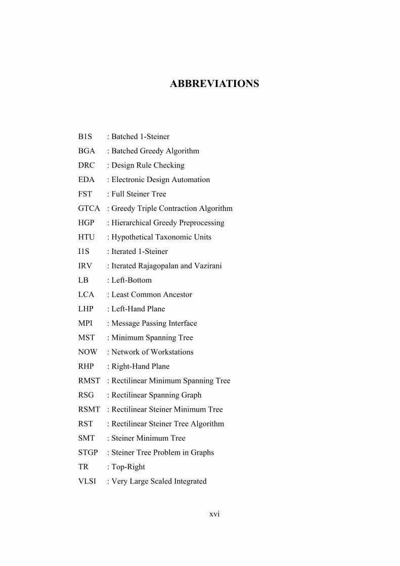
ABBREVIATIONS

B1S : Batched 1-Steiner

BGA : Batched Greedy Algorithm

DRC : Design Rule Checking

EDA : Electronic Design Automation

FST : Full Steiner Tree

GTCA : Greedy Triple Contraction Algorithm

HGP : Hierarchical Greedy Preprocessing

HTU : Hypothetical Taxonomic Units

I1S : Iterated 1-Steiner

IRV : Iterated Rajagopalan and Vazirani

LB : Left-Bottom

LCA : Least Common Ancestor

LHP : Left-Hand Plane

MPI : Message Passing Interface

MST : Minimum Spanning Tree

NOW : Network of Workstations

RHP : Right-Hand Plane

RMST : Rectilinear Minimum Spanning Tree

RSG : Rectilinear Spanning Graph

RSMT : Rectilinear Steiner Minimum Tree

RST : Rectilinear Steiner Tree Algorithm

SMT : Steiner Minimum Tree

STGP : Steiner Tree Problem in Graphs

TR : Top-Right

VLSI : Very Large Scaled Integrated

1

Equation Chapter (Next) Section 1

CHAPTER 1

INTRODUCTION

The Steiner Tree problem is one of the oldest optimization problems in graph theory

literature. It has many application areas one of which is the VLSI physical design

process. The rectilinear version of the Steiner Tree problem is used in VLSI

physical design because all nets are defined horizontally or vertically in this field

and the Rectilinear Steiner Tree Problem finds an interconnection of a net by using

only vertical and horizontal wires. It is different from the well studied rectilinear

minimum spanning tree (RMST) problem, which looks for the minimal total length

tree for a given set of vertices. The rectilinear Steiner minimum tree (RSMT)

achieves the possible minimum tree by using some extra points that are not in the

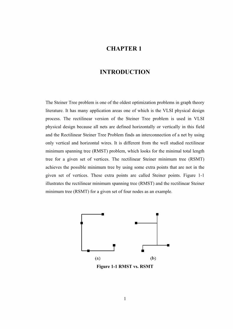
given set of vertices. These extra points are called Steiner points. Figure 1-1

illustrates the rectilinear minimum spanning tree (RMST) and the rectilinear Steiner

minimum tree (RSMT) for a given set of four nodes as an example.

Figure 1-1 RMST vs. RSMT

2

Following the developments in the VLSI field, the designs became very complex

and the number of transistors used in the designs has doubled every two years by

the famous Moore’s law. This brought up the result that up to millions of terminals

need to be connected in a minimum rectilinear path. It is worth noting that the

rectilinear Steiner minimum tree is calculated lots of times in a typical VLSI design

cycle. Since lots of electronic designs exist involving this number of terminals and

this number continuing to increase everyday, an efficient algorithm is needed to be

found. However it has been shown that the rectilinear Steiner minimum tree is NP-

complete. This result shows that the possibility of finding an efficient exact

algorithm to solve this problem is not known, at least with our current state of

knowledge. This leads the way to search for heuristic algorithms that solves the

problem approximately. Most of the heuristics proposed up to now uses rectilinear

minimum spanning tree as an initial step because it has been demonstrated that the

length of the RMST is at most 1,5 times longer than the RSMT and it can be

computed in polynomial time.

Although the rectilinear Steiner minimum tree has taken special interest, the

algorithms proposed until a few years ago did not fulfill the rising requirements.

Therefore several researchers have aimed at developing scalable algorithms but

there still seems to be a lack of parallel algorithms in this field.

In this thesis work, first a detailed survey on rectilinear Steiner minimum tree

problem has been presented. The major heuristics as well as exact algorithms that

are developed until now have been examined. The algorithms have been compared

mainly in terms of their performance and their time complexity. The performance of

the heuristics is given mostly in terms of their improvements to the MST.

Following the literature survey, two recently proposed heuristic algorithms have

been identified as efficient and satisfactory for relatively large input sizes. These are

Kahng, Mandoiu and Zelikovsky’s BGA algorithm [1] and Zhou’s RST algorithm

[2]. The other reason for selecting these two algorithms is the potential for their

parallel implementation in a distributed environment.

3

The main contributions of this study can be listed as follows:

- The thesis conducts a comprehensive literature survey on RSMT.

- It proposes a hybrid approach for solving the RSMT by modifying the

Zhou’s RST algorithm with some parts borrowed from Kahng et.al.’s BGA

algorithm.

- It proposes a partially distributed version of the modified algorithm.

- Following the implementation of the three algorithms, i.e., RST, BGA and

modified RST, comparisons on their performances and convergence times

are presented. The proposed modification approach, which is based on both

analysis and profiling results of the two known algorithms, has proved to be

effective.

- The proposed distributed algorithm is also implemented using the MPI

(message passing interface) middleware and the results of comparative tests

conducted on a cluster of workstations have been presented. The proposed

distributed algorithm has also proved to be promising and useful especially

for large problem instances.

This thesis work has been organized as follows:

In Chapter 2, the Steiner Tree Problem is defined and the historical background of

the problem is briefly given. Then different variations of the problem are presented

and the chapter ends by stating some application areas of the Steiner trees.

In Chapter 3, VLSI physical design cycle, which is one of the most important

application areas of Steiner trees, is reviewed. Since rectilinear Steiner trees are

heavily used in the physical design of VLSI systems, studying the Steiner trees and

consequently improving the VLSI physical design cycle is among the main

motivations and major interests of this thesis work.

In Chapter 4, the fundamental properties of rectilinear Steiner trees are defined

including the basic definitions used in the literature. Then the exact algorithms are

reviewed first, summarizing the main ideas that have created them. Afterwards

4

starting from the simplest algorithm, important heuristics are explained briefly. A

comparison of the reviewed heuristics is given and the purpose of selecting the

BGA and RST algorithms in this thesis is stated.

Chapter 5 first describes and explains in detail the components that form the BGA

algorithm. Secondly, it repeats the same type of decomposition for the RST

algorithm and it proposes the Modified RST algorithm finally.

In Chapter 6, parallel computing basics and a distributed environment are

introduced first. Then the modified RST algorithm components, which can be

parallelized, are discussed and the adopted method of parallelization is presented.

In Chapter 7, the data structures used in the implementations are explained. Then

the implementation results of sequential BGA, RST and the Modified RST are

presented. Chapter 7 also gives the implementation results of the distributed version

of the Modified RST.

Chapter 8 concludes the thesis work.

5

Equation Chapter 1 Section 1

CHAPTER 2

THE STEINER TREE PROBLEM

2.1. Problem Description

The Steiner problem asks for a shortest tree network spanning a given set of points

but it is different from the classical minimum spanning tree problem in which all

connections are required to be between the given set of points. The novel property

of Steiner tree problem is that new points other than the original points can be

introduced making the spanning tree as short as possible. These new points are

called Steiner points and the inclusion of these extra points makes the construction

of Steiner tree an NP-hard problem.

2.2. Historical Background of Steiner Tree Problem

The historical background of the Steiner Tree Problem goes to 1600’s. Fermat

proposed the problem of finding a point in the plane, the sum of whose distances

from three points is minimal. Torricelli proposed a geometric solution to this

problem before 1640. The general Fermat problem, which seeks a point in plane the

sum of whose distances from n given points is minimal, has attracted the attention

of many well-known mathematicians including Jacob Steiner [3].

In 1934 Jarnik and Kössler [4] raised the following question in a Czech journal:

Find a shortest network which interconnects n points in the plane?. But they did not

give any reference to Fermat.

6

Courant and Robbins first made the connection that the Fermat problem is the

shortest interconnection network with n=3 [5]. They have called the former Fermat

problem as ‘Steiner problem’ and called the Jarnik and Kössler problem as ‘street

network problem’. The popularity of their book made the problem called as the

Steiner problem afterwards.

Melzak established many basic properties of a shortest interconnecting network and

gave a finite solution to the Steiner problem [6]. Gilbert and Pollak introduced the

name Steiner minimal trees (SMT) for shortest interconnecting networks and

Steiner points for vertices of an SMT that are not among the n original points [7].

2.3. Variations of Steiner Tree Problem

There are many variations of the Steiner Tree problem for different metrics. These

different variations emerged from different types of applications. Some special

geometrical properties can be taken into account for special metrics.

Let ( , )x yu u u= and ( , )x yv v v= be a pair of points. The distance in the Lp metric,

where 1 p≤ ≤∞ , between u and v is ( )1/ pppx x y yp

uv u v u v= − + − . As special

cases L1-distance (called as rectilinear or Manhattan distance) equals to

( )1 x x y yuv u v u v= − + − and L2-distance (called as the Euclidean distance)

equals to 22

2 x x y yuv u v u v= − + − .

Three major versions have emerged for the Steiner tree problem. These are the

Euclidean Steiner problem, the Rectilinear Steiner problem and the Steiner problem

in networks. It can be shown that Steiner points in the Euclidean and the Rectilinear

cases belong to a finite set of points [3]. The Euclidean and the Rectilinear cases

can be thought as special cases of the network problem. The Euclidean Steiner

problem was the first identified version of the problem as was introduced in the

previous Section 2.2. The rectilinear Steiner problem is identified by Hanan in 1966

7

[8] and the Steiner problem in networks is defined by Hakimi in 1971 [9] as a

combinatorial version of the Euclidean Steiner problem. Other versions such as

octilinear Steiner minimum tree are defined afterwards.

Other variations also exist. One of them is the k-SMT where the Steiner minimum

tree spans exactly k points. Also Steiner Arborescence problem is defined as a

directed tree rooted at the origin, spanning all the given points. Another version of

the problem is the group Steiner tree problem, which is a generalization of the

Steiner tree problem where several subsets of vertices are given in a weighted graph,

where the goal is to find a minimum-weight connected sub-graph containing at least

one vertex from each group.

Although the above variations are among the most popular ones, other versions are

still possible and extensive surveys on the subject exists (for example [3]).

2.4. Application Areas of Steiner Trees

The Steiner tree problem is one of the most popular graph problems. Its popularity

depends on the fact that it has many application areas some of which are given

below.

One application of the Steiner tree stems from the minimal network theory.

Minimal networks are applied in many other fields such as cluster theory,

calculation of the characteristic dimension of a point set and minimization of the

length of conductors for electronic equipment manufacture. The most popular

problem in minimal network theory is finding the absolute minimal networks

spanning a given set of points. It is shown that any absolute minimal network

spanning a fixed set of points of the plane including some additional points is

always a tree and this tree is known as Minimal Steiner Tree [10].

Another application area arising from the network theory is the Quality of Service

Multicast Tree Problem, which appears in the context of multimedia multicast and

8

network design [11] and which is a generalization of the Steiner tree problem. The

aim of Multicast Routing is to efficiently interconnect a set of destinations in a

network for group communications like teleconferences. The resulting sub network,

known as a multicast tree, avoids unnecessary duplication of data while optimizing

a cost parameter such as bandwidth.

Other applications can also be found in different fields of science such as biology.

A phylogenetic tree is a tree showing the evolutionary interrelationship among

various species or other entities that are believed to have a common ancestor. In a

phylogenetic tree, each node with descendants represents the most recent common

ancestor of the descendants and edge lengths correspond to time estimates. Each

node in a phylogenetic tree is called a taxonomic unit. Internal nodes are generally

referred to as Hypothetical Taxonomic Units (HTUs) as they cannot be directly

observed [12]. These internal nodes correspond to Steiner points.

There may be several other applications of Steiner trees but the most important one

is its use in VLSI design. The next chapter presents the concepts of VLSI design

very briefly, to illustrate the motivations behind this thesis work.


9

CHAPTER 3

VLSI PHYSICAL DESIGN AUTOMATION

3.1. VLSI Design Problem

Very Large Scale Integration (VLSI) refers to those integrated circuits that contain

more than 105 transistors [13]. Since the VLSI chips today can contain more than a

hundred million transistors, a research field called electronic design automation

(EDA) has emerged. EDA is concerned with the tools that are used in the design

and production of VLSI systems.

In creating a VLSI system, six major steps have to be followed [14]. In specification

phase, a functional specification of the system under development is produced. In

logic design phase, the functional specification is transformed into a logical

representation. In circuit design phase, the logic representation is converted to

circuit elements like gates or standard cells. The physical design phase translates the

circuit design into a physical package representation also known as the layout. In

fabrication phase, the physical package representation is used to generate an actual

integrated circuit. In testing phase, the manufactured integrated circuit is examined

to determine whether there are manufacturing errors that prevent the integrated

circuit to work correctly in accordance with the functional specification.

VLSI Physical Design phase is within the scope of the current thesis work.

10

3.2. VLSI Physical Design Problem

The input to the physical design cycle is a circuit diagram and the output is the

layout of that circuit. It is accomplished by converting each logic component into a

geometric representation. Geometrical representation identifies the dimension and

location of the transistors and wires on a silicone surface [15]. Layouts of the

designs that need high performance may be partially manual designed but layouts of

most designs are automated. To efficiently solve the problem with automated

methods, physical design is accomplished in several stages main properties of

which are introduced in the following sections.

3.2.1. Circuit Partitioning

A chip can contain several millions of transistors, so it may not be possible to layout

the entire chip at one single step. Therefore the entire chip is normally partitioned

into sub-blocks. The partitioning process considers many factors such as the size of

blocks, the number of blocks and the number of interconnections between the

blocks. The output of partitioning is a set of blocks and the interconnections

required between the blocks [16].

3.2.2. Floorplanning and Placement

Floorplanning is concerned with selecting good layout alternatives for each block

coming from the previous step. The area can be estimated approximately for each

block after partitioning. This step is very critical because it constructs the basis for a

good layout. During the placement step the blocks are exactly positioned on the

chip. The goal of partitioning is to find a minimum area arrangement for the blocks

while meeting the performance constraints. The placement is done in two phases. In

the first phase an initial placement is created. In the second phase, the initial

placement is evaluated and iterative improvements are made until layout has

minimum area or best performance conforming the design specifications [16]. The

quality of placement will be determined after the routing is performed.

11

3.2.3. Routing

The objective of the routing phase is to complete the interconnections between

blocks according to the specified net list. First, the space that is not occupied by the

blocks is partitioned into rectangular regions. A router completes all

interconnections with shortest possible wire length using only rectangular regions.

The vertices of this grid graph represent potential pins and vias and the edges

represent the capacity of a channel, which can be defined as the routing space

between two channels [15]. The routing is realized in two phases called Global

Routing and Detailed Routing. In global routing phase, connections are made

between blocks but the details of each wire and pin are not taken into account.

Alternatively, the global routing is said to specify the different regions in the

routing space, which a wire should be routed. Then the point-to-point connections

between pins on each block is completed [16] in detailed routing.

3.2.4. Layout Compaction

Compaction phase can be identified by the task in which the layout is compressed in

all directions such that the total area is reduced. By making the chip even smaller

wire lengths are reduced, which in turn reduces the capacitances emerging from

long wires and so the signal delay. By reducing the area also the number of chips

produced from a wafer is increased, which may mean a significant cost decrease.

3.2.5. Extraction and Verification

This is a phase which checks the correctness of the layout. The Design Rule

Checking (DRC) is a process which verifies that all geometric patterns meet the

design rules imposed by the fabrication process [16]. After removing the design rule

violations, the functionality of the layout is verified by circuit extraction which is a

reverse engineering process. It generates a circuit from the layout to compare with

the original net list. In performance verification phase the geometric information to

compute resistance, capacitance, delay, etc is checked.

12

It is worth noting that physical design is an iterative process. That is to say, many

phases such as global routing and detailed routing are repeated several times to

obtain a better output. The quality of the design in some phase heavily depends on

the quality of the solution obtained in earlier phases. For example if a poor quality

solution is offered in the placement phase, even a high quality routing may not

produce a satisfactory and good result. In general whole design phases may be

repeated several times to accomplish the objectives of the design.

3.3. Using Rectilinear Steiner Trees in VLSI Physical Design

Problem

After defining the major concepts of VLSI physical design in the previous section,

this section will answer the question of ‘where does the Steiner tree problem fit in

the physical design process?’.

It has to be noted again that the geometry of VLSI, which usually allows only

vertical and horizontal wiring directions, has motivated the studies of the rectilinear

version of the problem [17]. The Steiner trees can be used in two phases of the

VLSI physical design process, namely the placement and global routing phases.

The quality of a placement solution is evaluated by estimating the total wire length

[13]. The total wire length is estimated by first estimating a length for each net and

then by summing them up. In the next step total wiring area can be derived from

this length by assuming a certain wire width and a wire separation distance. For

timing critical nets, the minimization of wire concept defined here is not enough,

but for most of the nets in a typical design is not that critical. Therefore, SMT can

be used as an accurate estimation of wire length for the placement phase and this

implies that the Steiner tree will be invoked millions of time [2].

The object of routing problem for a general purpose chip is to minimize the total

wire length [16]. This is because VLSI design rules dictate a minimum separation

13

between wires and therefore the area occupied by the routing on a chip is roughly

proportional to the total wire length of the routing [17]. Added wire length generally

increases signal delay and power consumption due to increased resistance and

capacitance. For global routing two types of nets exists; two terminal nets and nets

with more than two terminals. Multi-terminal nets can be formulated as Steiner tree

problems [3]. The size of the nets becomes larger with the improvements in the

VLSI technology, so does the size of the Steiner trees involved.

In Chapter 2, Steiner tree problem has been defined and in this chapter one

important use of the rectilinear Steiner tree problem is stated. The next section will

investigate the problem in more detail by giving its properties and the algorithms

that solve it.


14

CHAPTER 4

THE RECTILINEAR STEINER TREE PROBLEM

4.1. Problem Description

Hanan is the first author who considered the rectilinear version of the Steiner tree

problem [8]. This version constitutes all definitions that have been made in the

Euclidean version of the problem but all distances are measured in rectilinear metric.

The rectilinear Steiner minimum tree (RSMT) is a tree that interconnects a set of

terminals consisting of horizontal and vertical line segments only while having

minimum total length [18]. This is equivalent to saying ‘construct a Steiner

minimum tree for the given set of terminals under the L1 metric’. Given two points

( , )x yu u u= and ( , )x yv v v= , the L1 distance between them is

x x y yuv u v u v= − + − . In other words, it is equal to the sum of distances in each

of the two dimensions.

The problem is proved to be NP-complete by Garey and Johnson [19]. They have

transformed the problem of node cover in planar graphs, which was proved to be in

NP-complete class earlier, to rectilinear Steiner minimum tree (RSMT)

polynomially [20]. Therefore no polynomial-time algorithm is found up to now for

this problem and more effort is given to heuristic solutions after this proof.

Some definitions and properties about Rectilinear Steiner Minimum Tree will be

given in the next section. Then some important exact algorithms and heuristics

proposed up to now will be investigated.

15

4.2. Definitions and Basic Properties

A rectilinear segment is a horizontal or vertical line segment connecting its two

endpoints in the plane. The intersection points of these segments are called nodes.

The degree of a node is the number of segments incident to it. The nodes are either

terminals (from the given set of points) or non-terminals. There are three types of

non-terminals. Corner points have degree two and thus have exactly two incident

perpendicular segments. T-points have degree three and cross points have degree

four. T-points and cross points are also called Steiner points. Corner points are not

defined as Steiner points because they do not have a distinct position on the tree.

Namely, if the point that is in the opposite diagonal of the corner point is included

on the tree; the length of the tree does not change. It can be noted that each endpoint

of a segment is a terminal, a Steiner point or a corner point.

A line of segments is defined as a sequence of one or more adjacent, collinear

segments with no terminal nodes in its relative interior. A complete line is defined

as a line of maximal length. A corner point is incident to exactly one horizontal

complete line and one vertical complete line where these complete lines are referred

as the legs of the corner. If the other endpoints of the legs are terminals, the corner

is referred as a complete corner.

A rectilinear Steiner tree in which every terminal is a leaf is called a Full Steiner

Tree (FST). It is found that every SMT is a union of FSTs. A fulsome SMT is

defined as an SMT in which the number of FSTs is maximized. The number of

FSTs is equals to ( )1 deg( ) 1z Z

z∈

+ −∑ where Z is the set of terminals and deg(z) is

the degree of a terminal z ∈ Z. Therefore it can be said that in a fulsome SMT, sum

of the degree of all terminals in the set is maximized.

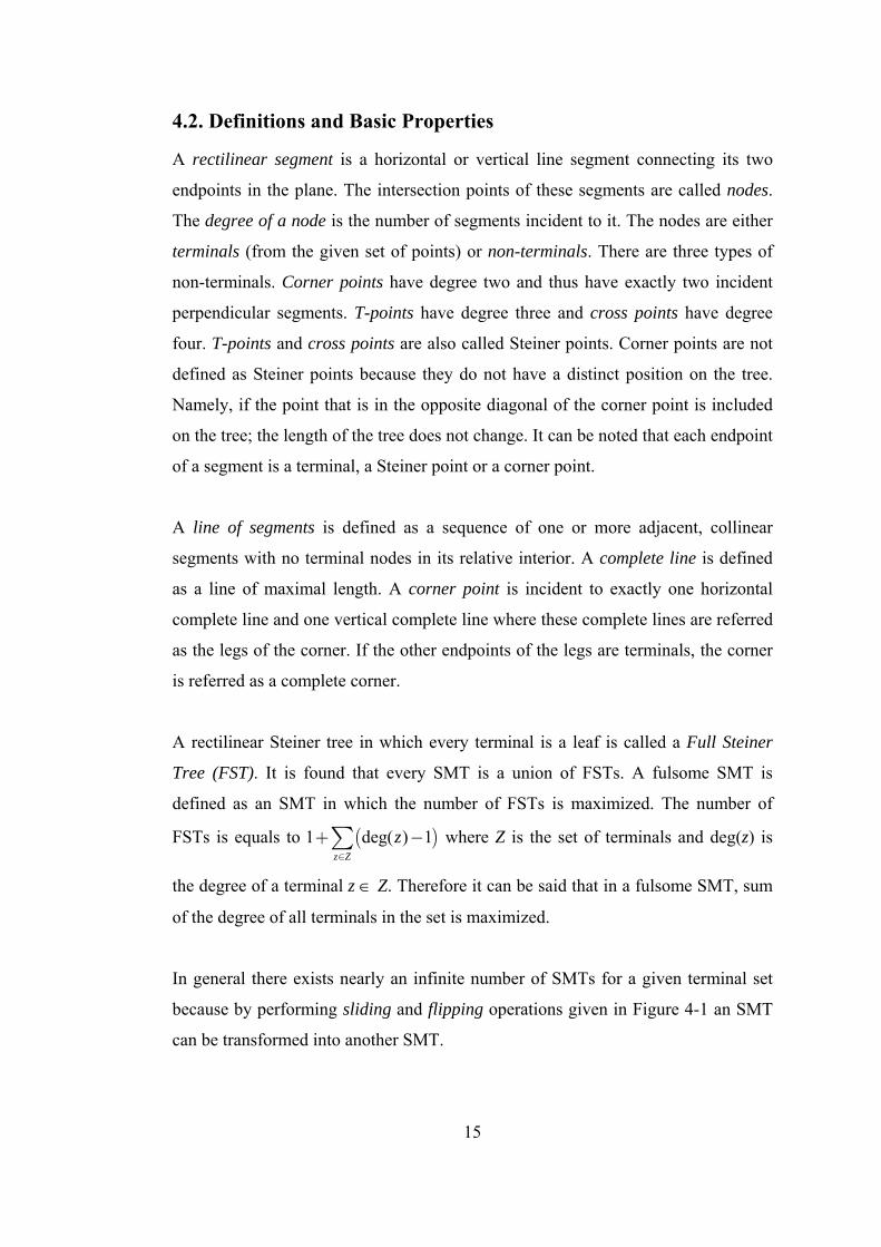
In general there exists nearly an infinite number of SMTs for a given terminal set

because by performing sliding and flipping operations given in Figure 4-1 an SMT

can be transformed into another SMT.

16

Figure 4-1 Sliding and Flipping Transformations

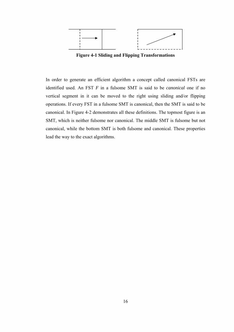
In order to generate an efficient algorithm a concept called canonical FSTs are

identified used. An FST F in a fulsome SMT is said to be canonical one if no

vertical segment in it can be moved to the right using sliding and/or flipping

operations. If every FST in a fulsome SMT is canonical, then the SMT is said to be

canonical. In Figure 4-2 demonstrates all these definitions. The topmost figure is an

SMT, which is neither fulsome nor canonical. The middle SMT is fulsome but not

canonical, while the bottom SMT is both fulsome and canonical. These properties

lead the way to the exact algorithms.

17

Figure 4-2 Fulsome and Canonical SMTs

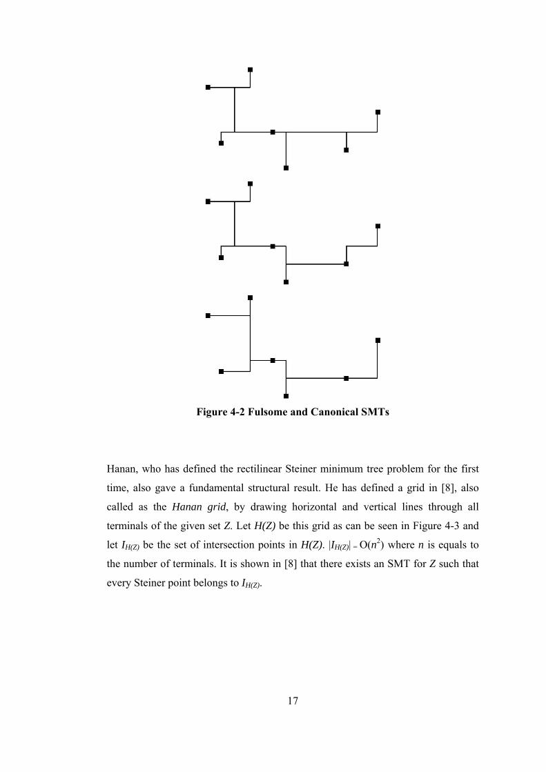
Hanan, who has defined the rectilinear Steiner minimum tree problem for the first

time, also gave a fundamental structural result. He has defined a grid in [8], also

called as the Hanan grid, by drawing horizontal and vertical lines through all

terminals of the given set Z. Let H(Z) be this grid as can be seen in Figure 4-3 and

let IH(Z) be the set of intersection points in H(Z). |IH(Z)| = O(n2) where n is equals to

the number of terminals. It is shown in [8] that there exists an SMT for Z such that

every Steiner point belongs to IH(Z).

18

Figure 4-3 Hanan Grid for a Set of Terminals

This result of Hanan can be interpreted as follows: only the intersection points in

the Hanan grid can be Steiner point candidates. This is a very important finding

because only a polynomial number of points need to be considered as possible

Steiner points. Another bound on the Steiner points is given by Gilbert and Pollak

[7] by proving that that any Steiner tree may contain at most n-2 Steiner points.

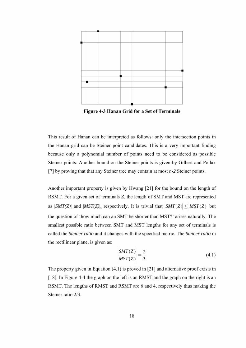
Another important property is given by Hwang [21] for the bound on the length of

RSMT. For a given set of terminals Z, the length of SMT and MST are represented

as |SMT(Z)| and |MST(Z)|, respectively. It is trivial that ( ) ( )SMT Z MST Z≤ but

the question of ‘how much can an SMT be shorter than MST?’ arises naturally. The

smallest possible ratio between SMT and MST lengths for any set of terminals is

called the Steiner ratio and it changes with the specified metric. The Steiner ratio in

the rectilinear plane, is given as:

( ) 2( ) 3

SMT ZMST Z

= (4.1)

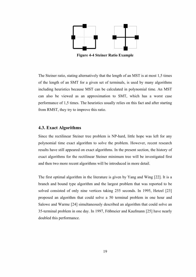
The property given in Equation (4.1) is proved in [21] and alternative proof exists in

[18]. In Figure 4-4 the graph on the left is an RMST and the graph on the right is an

RSMT. The lengths of RMST and RSMT are 6 and 4, respectively thus making the

Steiner ratio 2/3.

19

Figure 4-4 Steiner Ratio Example

The Steiner ratio, stating alternatively that the length of an MST is at most 1,5 times

of the length of an SMT for a given set of terminals, is used by many algorithms

including heuristics because MST can be calculated in polynomial time. An MST

can also be viewed as an approximation to SMT, which has a worst case

performance of 1,5 times. The heuristics usually relies on this fact and after starting

from RMST, they try to improve this ratio.

4.3. Exact Algorithms

Since the rectilinear Steiner tree problem is NP-hard, little hope was left for any

polynomial time exact algorithm to solve the problem. However, recent research

results have still appeared on exact algorithms. In the present section, the history of

exact algorithms for the rectilinear Steiner minimum tree will be investigated first

and then two more recent algorithms will be introduced in more detail.

The first optimal algorithm in the literature is given by Yang and Wing [22]. It is a

branch and bound type algorithm and the largest problem that was reported to be

solved consisted of only nine vertices taking 255 seconds. In 1995, Hetzel [23]

proposed an algorithm that could solve a 50 terminal problem in one hour and

Salowe and Warme [24] simultaneously described an algorithm that could solve an

35-terminal problem in one day. In 1997, Fößmeier and Kaufmann [25] have nearly

doubled this performance.

20

All these algorithms were based on the same method that was suggested by Winter

[26] for the Euclidean Steiner tree problem in the plane. This method is adopted to

the rectilinear case. It uses the fact that there exists an SMT, which is a union of

FSTs having Hwang topology, which is described in Section 4.3.2.1. Thus first,

they generate all Full Steiner Trees that could have been found in the terminal set.

Then they concatenate these trees in order to form a rectilinear Steiner minimum

tree. The major bottleneck of the algorithm was the concatenation phase until

Warme [27] introduced a major breakthrough in the process.

In the next section the properties that an algorithm has to satisfy in order to be

optimal will be discussed. Then the fastest algorithm that has been designed until

now will be introduced. And Hanan Grid based algorithms will be explained

afterwards.

4.3.1. Necessary Optimality Conditions

An edge e= (u, v) in a Steiner minimum tree is a direct connection between a pair of

nodes u and v, which are either terminal or Steiner points. In fulsome and canonical

SMT an edge is either a single segment or a pair of perpendicular segments adjacent

at a corner point. The length of it is calculated in rectilinear metric and called ||e||. It

is also worth noting that any sub-tree of an SMT must be an SMT for the nodes that

it spans and the same condition occurs for FST. Now some upper bounds about the

length of edges in MST will be discussed.

Consider an SMT and two terminals called i and j. The unique path between i and j

in the SMT is denoted by P(i, j). If any edge called e on this path is removed from

SMT, the tree will be broken into two connected components. Now an edge in the

MST, say f, will reconnect these broken components. Clearly these edges have to

satisfy e f< since otherwise SMT will not be optimal. Therefore the bottleneck

Steiner distance, bi,j, between a pair of terminals i and j is equal to the length of the

longest edge in the MST between i and j [3]. After identifying the bottleneck

21

Steiner distance, it can be proved that for any edge e ∈ P(i, j) in the SMT the

rectilinear length of ||e|| must be smaller from bi,j.

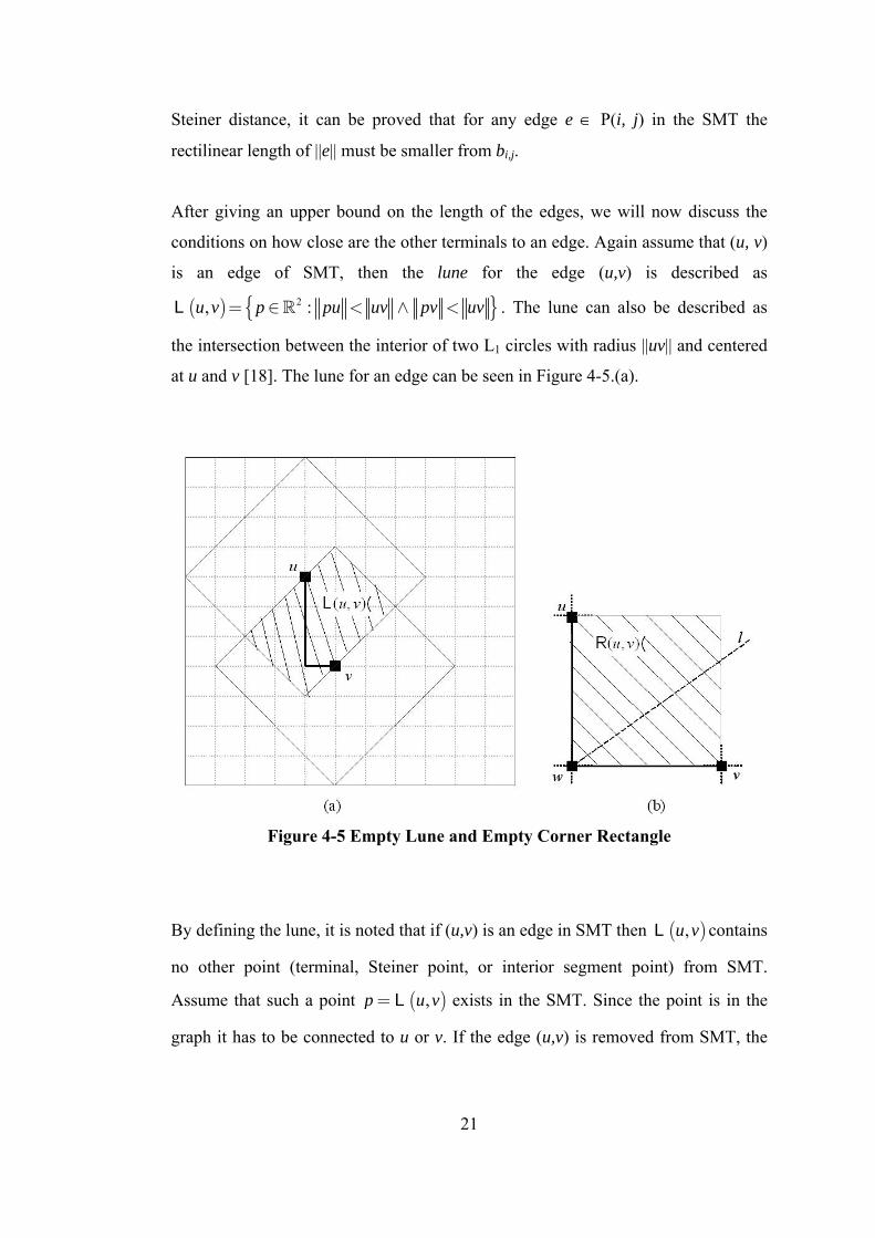
After giving an upper bound on the length of the edges, we will now discuss the

conditions on how close are the other terminals to an edge. Again assume that (u, v)

is an edge of SMT, then the lune for the edge (u,v) is described as

( ) { }2, :u v p pu uv pv uv= ∈ < ∧ <R L . The lune can also be described as

the intersection between the interior of two L1 circles with radius ||uv|| and centered

at u and v [18]. The lune for an edge can be seen in Figure 4-5.(a).

Figure 4-5 Empty Lune and Empty Corner Rectangle

By defining the lune, it is noted that if (u,v) is an edge in SMT then ( ),u vL contains

no other point (terminal, Steiner point, or interior segment point) from SMT.

Assume that such a point ( ),p u v= L exists in the SMT. Since the point is in the

graph it has to be connected to u or v. If the edge (u,v) is removed from SMT, the

22

edge will be split into two connected components and one component will contain

the point p. Supposing that the component that have point u contains point p also,

by adding edge (p,v) the length of the SMT will be reduced which results in a

contradiction. Therefore the lune has to be empty.

If two nodes u, v are not directly connected with an edge, but with another node, say

w, such that the segments uw and wv are perpendicular as in Figure 4-5.(b), ( ),u vR

can be defined as the interior of the rectangle with sides uw and wv and then no

other point can exist in ( ),u vR . This can be proved by assuming again that there

exists such a point ( ),p u v= R . Let l be a line that passes through w and assume

that p lies above the line l. Then when the edge (u,w) is removed from SMT, two

connected components are formed. If p was connected to u before the deletion

operation the SMT will be shortened by adding an edge from p to the segment wv,

which is a contradiction.

4.3.2. Geosteiner

The GeoSteiner algorithm [28] depends on the method that was suggested by

Winter [26] for the Euclidean Steiner tree problem in the plane as it was mentioned

below. It uses the fact that there exists an SMT, which is a union of FSTs having

Hwang topology. Thus first, they generate all Hwang topology Full Steiner Trees

that fulfills the necessary optimality conditions. Then a subset of these FST’s is

selected in the concatenation phase.

4.3.2.1. FST Generation

It can be noted that FST concatenation phase was computationally harder than the

FST generation phase. However, after Warme have introduced an effective way of

concatenating the FSTs [27], the FST generation phase then posed an overhead to

the whole algorithm. Therefore, a new method is also proposed by Zachariasen for

FST generation phase [29].

23

Hwang [21] has proven that every FST in a canonical and fulsome SMT has a very

particular shape denoted as the Hwang topology. The FSTs have one of the two

generic shapes, and two degenerate cases, which can be seen in Figure 4-6 and can

be stated as follows: An FST spanning k terminals consists of a corner (also denoted

as the backbone) given by root z0 and a tip zk-1. The root is incident to the long leg,

and the tip is incident to the short leg. Here long leg means, it has more incident

segments than the short leg. There are two main types (i) and (ii) and two

degenerate cases of type (i) [18]:

- Type (i) has k-2 alternating segments incident to the short leg. The first

degenerate case (i’) has a zero-length short leg, that is, the corner is

degenerated into a line. The second degenerate case (ii’) is a cross spanning

exactly four terminals.

- Type (ii) has k-3 alternating segments incident to the long leg and one

segment incident to the short leg.

Figure 4-6 Hwang topology FSTs

24

The FSTs that are generated from the algorithm are all Hwang-topology FSTs. The

algorithm works by growing FSTs. For a given terminal z0 and a specific direction,

an FST is grown out with long leg being in the specified direction. Let the growing

direction be East and an example growing algorithm can be stated as follows:. All

terminals to the right of the vertical line through z0 are sorted by their x-coordinate.

Also Za and Zb denote the list of sorted terminals that are above the horizontal line

through z0 and the list of sorted terminals that are below this line respectively. By

using the necessary optimality conditions and by selecting one terminal from Za and

then from Zb the algorithm saves the FSTs and recursively continues. It must be

noted that the algorithm also backtracks if the optimality conditions can not be

satisfied.

An independent preprocessing phase for FST generation, which runs in O(n2) time,

is given in [29]. The main purpose of this algorithm is reducing the set of terminals

that can be attached to a backbone. Bottleneck Steiner distances, empty lunes and

empty corner rectangles are used to eliminate long-leg and short-leg terminal

candidates which will reduce the overall complexity of the algorithm.

4.3.2.2. FST Concatenation

Warme gave an algorithm for finding the MST for the hypergraph problem [27]. He

has motivated this algorithm to the FST concatenation phase. A hypergraph is

generated with the set of terminals as its vertices and the generated FST in the

previous step as its hyperedges. It has been shown in [27] that this problem is NP-

hard when the hypergraph contains edges of cardinality four or more. Some

methods to solve this problem have been tried in [28] such as backtrack search,

dynamic programming or integer programming. Warme already gave an integer

programming (IP) formulation, which is used in his branch-and-cut method. His IP

formulation depends on three facts. First one is that the total length of the selected

hyperedges has to be small. Then the hyperedges have to span all edges and the

final one is that the resulting graph will have no cycles. The GeoSteiner code can be

found in [30].

25

Later Emanet [31] has also proposed a new method for this concatenation phase by

applying some modifications on Warme’s ideas.

4.3.3. Hanan Grid Based Exact Algorithms

The first algorithms for the Rectilinear Steiner Tree Problem were based on the

result that there exists an SMT in the Hanan grid that is composed for the given set

of terminals. Hanan shown that RSTP problem reduces to Steiner Tree Problem in

Graphs (STGP), which is stated as follows: Given an edge-weighted graph G=(V,E)

and a set of terminals Z V⊆ , find a tree in G that interconnects Z and has minimum

total length [18].

The best algorithm proposed for this problem up to now uses an IP formulation [32].

The algorithm first generates a directed graph having the same vertices as G; where

for every edge of G there are two directed edges and both of these edges costs as the

edge in G. Then by selecting an arbitrary terminal as root, the problem changes into

finding a rooted directed tree of minimum total length that contains all terminals,

which is also called a Steiner arborescence [18].

The algorithm mentioned above uses the complete Hanan grid so it has problem

when the number of terminals are more than 40. But the Hanan grid can be

simplified first to improve its performance. Techniques of such reductions are

presented in [33].

4.4. Approximation Algorithms

Since the Rectilinear Steiner Tree Problem is NP-hard, the major research effort is

given to heuristic approximation algorithms. Having shown also that the rectilinear

minimum spanning tree is at most 1,5 times longer than the rectilinear Steiner

minimum tree, most of the heuristics starts with MST and tries to improve it. In the

following, MST Embedding will be shown first and then the heuristics that improve

the Steiner ratio from 3/2. Next, B1S and IRV heuristics, which add Steiner points

26

to the MST iteratively, will be introduced. Afterwards Borah’s algorithm, which

updates edges of MST iteratively and BGA algorithm, which merges tiny optimal

Steiner trees to MST will be presented. And finally the RST algorithm, which

improves Borah’s algorithm with the help of the spanning graphs will be given.

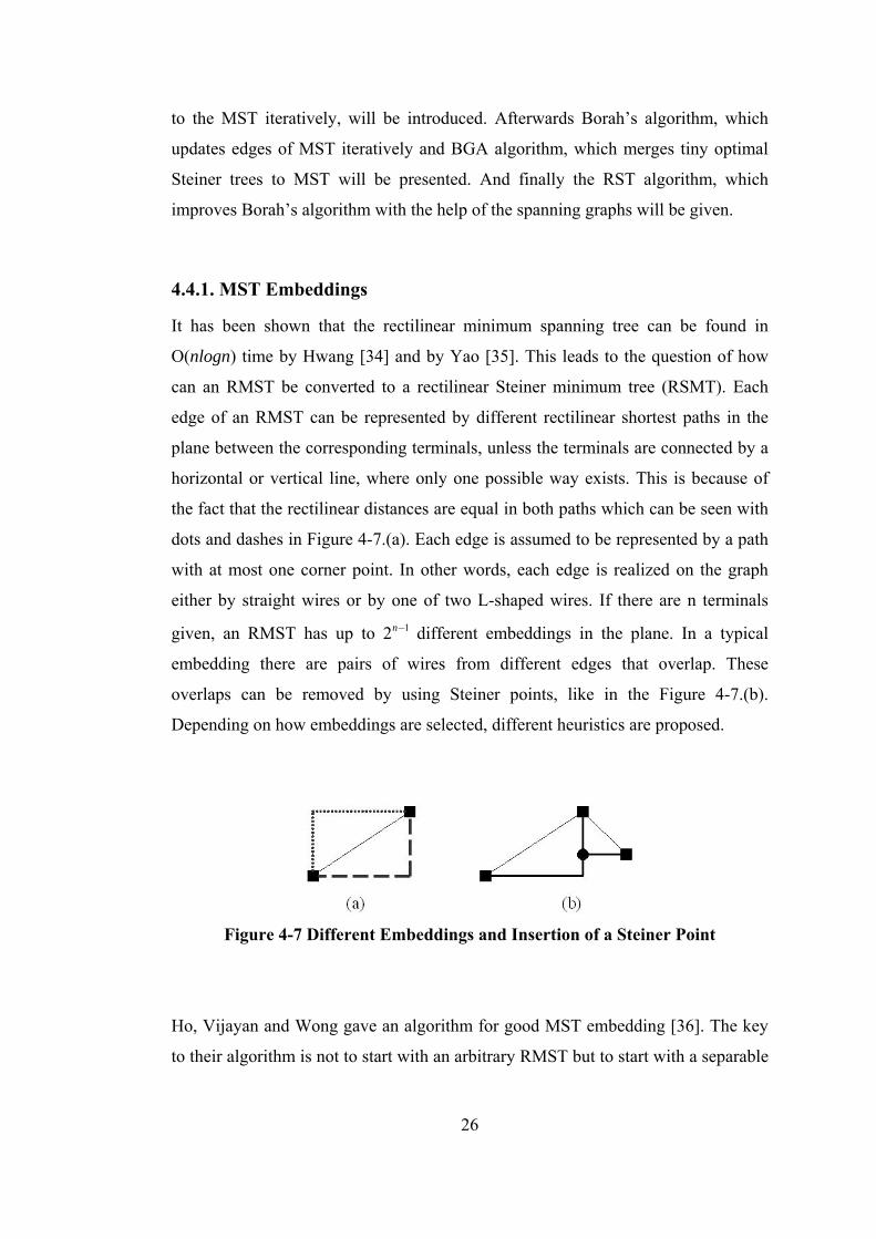
4.4.1. MST Embeddings

It has been shown that the rectilinear minimum spanning tree can be found in

O(nlogn) time by Hwang [34] and by Yao [35]. This leads to the question of how

can an RMST be converted to a rectilinear Steiner minimum tree (RSMT). Each

edge of an RMST can be represented by different rectilinear shortest paths in the

plane between the corresponding terminals, unless the terminals are connected by a

horizontal or vertical line, where only one possible way exists. This is because of

the fact that the rectilinear distances are equal in both paths which can be seen with

dots and dashes in Figure 4-7.(a). Each edge is assumed to be represented by a path

with at most one corner point. In other words, each edge is realized on the graph

either by straight wires or by one of two L-shaped wires. If there are n terminals

given, an RMST has up to 12n− different embeddings in the plane. In a typical

embedding there are pairs of wires from different edges that overlap. These

overlaps can be removed by using Steiner points, like in the Figure 4-7.(b).

Depending on how embeddings are selected, different heuristics are proposed.

Figure 4-7 Different Embeddings and Insertion of a Steiner Point

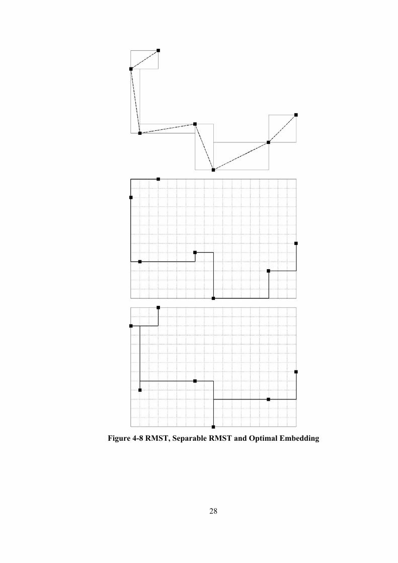
Ho, Vijayan and Wong gave an algorithm for good MST embedding [36]. The key

to their algorithm is not to start with an arbitrary RMST but to start with a separable

27

RMST. This is an MST for which the bounding boxes only overlap if the

corresponding edges share a terminal. This definition can be made clear by the

Figure 4-8. In the uppermost figure, overlapping bounding boxes can be seen. The

middle figure shows an MST where no line segments overlap, which is the case for

the separable MST. And also at the bottommost figure an optimal embedding can be

seen. They have also proven that such an MST can be constructed in O(nlogn) time.

28

Figure 4-8 RMST, Separable RMST and Optimal Embedding

29

They have shown that starting with a separable MST; an optimal L-shaped

embedding can be constructed in O(n) time. They have satisfied this with a O(n)

time dynamic programming algorithm. They have begun by rooting the separable

RMST at some leaf terminal and solve the sub-trees bottom-up. The key

observation of the algorithm is that with a separable RMST, the optimal solution for

a sub-tree depends only on the choice of which of the two embeddings of the L-

shaped wire connecting the root of the sub-tree to its parent was chosen. It is worth

noting that an optimal embedding for a given RMST is not necessarily an RSMT.

It can be shown that L-shaped wires are insufficient to find the optimal embeddings

[3]. So Z-shaped wires, which have two corner points are also offered in [36]. Z-

shaped optimal embeddings can achieve good improvements in O(n2) time

generally but the worst case running time is O(n7).

4.4.2. Zelikovsky Based Heuristics

As it was noted before the rectilinear minimum Steiner tree is at most 3/2 times the

rectilinear Steiner minimum tree. Zelikovsky worked generally on improving this

ratio. He has improved this ratio to 11/6 and 11/8 [37, 38]. The algorithm proposed

in [38] runs in O(n3) time and guarantees a performance of ratio 11/8. Afterwards

Berman and Ramaiyer improved this time complexity to O(n5/2) [39] and finally

Fößmeier has given a new time bound of O(n3/2) [40].

The main idea of the algorithm is to start with an initial rectilinear minimum

spanning tree and then iteratively computing optimal Steiner trees for small subset

of terminals and inserting these small Steiner trees into the current tree. In the

algorithm 3-restricted full Steiner trees will be used, since the computation of

bigger trees will be more complex than this one. A 3-restricted Steiner tree is

composed of FST’s each having at most 3 terminals. In the algorithm these small

trees are called stars and it is proven that O(n) stars will be enough to achieve 11/8-

approximation ratio. Also a method of finding O(n) stars in O(nlog2n) time has been

introduced in the paper.

30

Arora has also proposed an approximation algorithm but this has mainly a

theoretical importance [41]. His algorithm, for any fixed value 0ε> , produces a

rectilinear tree whose length is within a factor of 1 ε+ from optimum. His paper

was actually a major breakthrough with its main focus on approximating the

Euclidean traveling salesman problem [18]. The algorithm consists of three phases,

which are perturbation, shifted quadtree construction and dynamic programming.

As it was noted before this algorithm has mainly a theoretical importance but it

offers a way to solve the problem in polynomial time with a performance nearly like

the optimum.

4.4.3. B1S and IRV Heuristics

Kahng and Robins [42] presented a heuristics called Iterated 1-Steiner (I1S) that has

been used the Rectilinear Steiner Tree Problem for long years [3]. This heuristic is

based on the 1-Steiner Tree problem, which looks for the optimal Steiner tree if at

most one Steiner point is permitted. This can alternatively be stated as follows: what

is the location of a single point p such that RMST of N ∩ {p} is minimized? By

taking this as a starting point, the I1S heuristic finds a set of Steiner points S such

that MST(Z∩S) has minimum length.

It has to be noted that the number of Steiner points can be at most n-2 [7] and also

the Steiner point candidates are only needed to be searched in the Hanan grid. Using

these facts the I1S method repeatedly finds 1-Steiner points and includes them in

the Steiner point set. This procedure continues until no points can be found that will

improve MST (P ∩ S) where P represents the initial terminal set and S represents

the Steiner point set. This procedure can add more than n-2 points so that at each

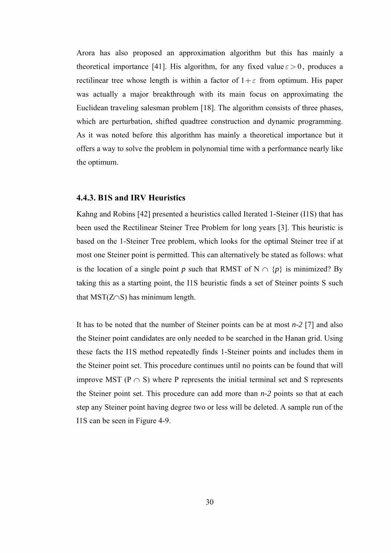
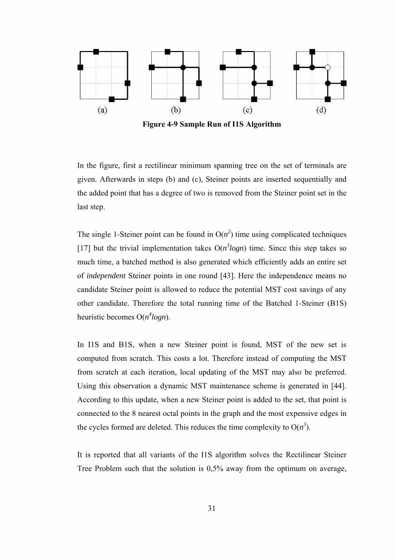
step any Steiner point having degree two or less will be deleted. A sample run of the

I1S can be seen in Figure 4-9.

31

Figure 4-9 Sample Run of I1S Algorithm

In the figure, first a rectilinear minimum spanning tree on the set of terminals are

given. Afterwards in steps (b) and (c), Steiner points are inserted sequentially and

the added point that has a degree of two is removed from the Steiner point set in the

last step.

The single 1-Steiner point can be found in O(n2) time using complicated techniques

[17] but the trivial implementation takes O(n3logn) time. Since this step takes so

much time, a batched method is also generated which efficiently adds an entire set

of independent Steiner points in one round [43]. Here the independence means no

candidate Steiner point is allowed to reduce the potential MST cost savings of any

other candidate. Therefore the total running time of the Batched 1-Steiner (B1S)

heuristic becomes O(n4logn).

In I1S and B1S, when a new Steiner point is found, MST of the new set is

computed from scratch. This costs a lot. Therefore instead of computing the MST

from scratch at each iteration, local updating of the MST may also be preferred.

Using this observation a dynamic MST maintenance scheme is generated in [44].

According to this update, when a new Steiner point is added to the set, that point is

connected to the 8 nearest octal points in the graph and the most expensive edges in

the cycles formed are deleted. This reduces the time complexity to O(n3).

It is reported that all variants of the I1S algorithm solves the Rectilinear Steiner

Tree Problem such that the solution is 0,5% away from the optimum on average,

32

and hence it can be called as the champion heuristic with respect to solution quality

performance [18].

More recently Mandiou et al.[45] have proposed a new heuristic, IRV, which is

similar to I1S concept. Similar to the previous ones, it also adds one or more points

to MST until the MST does not improve, but it identifies the Steiner point

candidates with a much more sophisticated algorithm. Their algorithm depends on

the ideas given in [46] and it performs a little better than B1S but slightly worse

when the empty rectangle test, which reduces the number of Steiner candidate

points in the Hanan grid, is used for B1S.

4.4.4. Borah’s Algorithm

The edge based heuristic that is proposed by Borah et al.[47] first calculates an

initial rectilinear minimum spanning tree. The algorithm improves the cost of this

MST by connecting a node to the rectangular layout of a neighboring edge and

removing the longest edge in the loop that is formed by this process. By a straight

forward implementation the complexity of Borah’s algorithm is O(n2). The

performance of the algorithm is shown to be close to the performances of other

more complex heuristics.

This algorithm will be explained in much detail in Section 5.2.2, therefore only its

general idea will be emphasized in the present section. In Figure 5-27 the basic

operation of the algorithm is shown. This algorithm shortens the length of the MST

by appending a terminal point to an edge in the MST. As a result a cycle is formed

and by deleting the most expensive edge in this cycle an improvement can be

achieved. The gain of this operation is positive if the cost between the terminal that

was appended and the Steiner point that is grown out after this operation is shorter

than the most expensive edge found in the cycle. It has to be noted that all costs are

computed in rectilinear metric.

33

In the straight forward implementation all terminals will be appended to all edges of

the MST. Thus the time complexity is O(n2) which is better than the previous

proposed heuristics. In the previous algorithms mostly new nodes were connected to

the graph, but in this heuristics edges are updated. Moreover it is mentioned in its

associated paper that the heuristic achieves this improvement with no degradation in

performance. It is noted that its performance, which is measured as the reduction of

the length of the MST, is in the range of Iterated 1-Steiner heuristic.

Besides the above straightforward implementation, another method is also offered

in [47]. First of all, for the initial minimum spanning tree phase they propose using

Hwang’s O(nlgn) time algorithm given in [34]. Then their new method relies on the

fact that for an edge under consideration, not all terminals have to be connected to

that edge. Considering only the terminals that are visible to the edge should be

sufficient. For a point-edge pair to be able to result in a positive gain when merging

into an MST, the point has to be visible to the edge meaning that there must be no

edge that exists in the path from the point to the edge. Although this new method

can result in a complexity of O(nlgn), it seems hard to implement it satisfactorily.

4.4.5. BGA

The BGA algorithm proposed by Kahng et. al. [1] starts with an initial minimum

spanning tree and iteratively improves it. It is claimed to run in O(nlg2n) time

producing high quality solutions. The BGA algorithm uses the implementations

proposed in [40] for the GTCA algorithm of Zelikovsky [37] with the batched

method introduced in [43].

In BGA algorithm, a sparse graph for initial minimum spanning tree computation is

constructed by using the Guibas-Stolfi algorithm [48]. This algorithm relies on the

fact that for the rectilinear metric a point can not be connected to two points in the

same octal region. In Guibas-Stolfi’s algorithm, first, all octal regions are mapped

into the first quadrant. Then with a recursive method, all north-east nearest

neighbors are found for all regions. Therefore all nearest points in all octal regions

34

are found and then Kruskal’s MST algorithm is used in order to obtain the final

rectilinear MST.

The GTCA algorithm finds an approximate minimum cost 3-restricted Steiner tree

by greedily choosing 3-restricted full components, which are called triples. When a

triple is merged into MST, two cycles are formed and then they are removed by

deleting the most expensive edges in each cycle. The gain of a triple is the

difference between two most expensive edges in each cycle formed and the cost of

the triple. A triple is called empty if the minimum rectangle bounding the triple

does not contain any other terminals and it is called a tree triple if the gain when the

triple is merged into MST is positive. In BGA algorithm all empty tree triples are

found and they are sorted according to the gains of the triples in non-increasing

order. Then the greedy rule used in GTCA is changed to batched method. This

means that starting from the triple with the biggest gain; all triples will be merged

into the MST if both most expensive edges for the triple are not deleted yet. Finally

all chosen triples will be applied to MST, the output being an approximate

minimum Steiner tree.

In BGA, a new methodology is also given for the triple generation phase. The

triples are divided into four types according to terminals’ geometrical position with

respect to each other. The terminals are partitioned recursively and four cases for

each type of triples are generated. With these methods all empty tree triples are

generated. The maximum number of such triples is O(n).

A maximum cost edge on the tree path is computed with a new method in BGA.

Two arrays are computed for this purpose, which have a maximum length of 2n.

These arrays are computed with a preprocessing algorithm, which runs in the same

time with Kruskal’s algorithm. This preprocessing algorithm takes O(nlgn) time

which is computed once. Then each maximum cost edge between two points is

calculated in O(lgn) time.

35

4.4.6. RST

The RST algorithm proposed by Zhou [2] is also a heuristic which starts with an

initial minimum spanning tree and iteratively improves it. This algorithm uses the

basis of Borah’s algorithm, which was introduced in Section 4.4.4. It is an enhanced

algorithm that uses the spanning graph introduced by Zhou et al. [49] among other

improvements. The algorithm runs in O(nlgn) time and takes O(n) storage without

losing the performance of Borah’s algorithm [2].

In Borah’s algorithm, point-edge pairs are formed and used. In the original

algorithm, all points in the given set are taken into account for all edges of the MST.

Borah has already pointed out that this is not necessary. A “spanning graph” is a

sparse graph in which a minimum spanning tree exists. Zhou noticed that a

spanning graph can be used to generate point-edge pairs although there is no direct

relationship with the visibility of the point and spanning graph. In Zhou’s RST

algorithm, for an edge in the MST, the neighbors in the spanning graph of the points

forming that edge are taken as point components of the corresponding point-edge

pair. Thus by forming point-edge pairs in this manner, O(n) point-edge pairs are

formed. This is because of the fact that a point can be connected to at most 8 octal

neighbors in the spanning graph. After a point-edge pair is updated in the MST, the

most expensive edge in the formed cycle is then found.

RST algorithm uses the spanning graph concept also in the initial MST computation

phase. The spanning graph depends on the octal partitioning concept. A point can

not be connected to two points in the same octal region for the rectilinear metric. A

sweep-line algorithm was designed by Zhou et al. [49] to generate the rectilinear

spanning graph.

After the spanning graph is generated, Kruskal’s algorithm is used to find the initial

rectilinear minimum spanning tree. Kruskal’s algorithm is used also in the longest

edge computation for all point-edge pairs. In Kruskal’s algorithm, the edges are

initially sorted with respect to their costs and this information is used for a least

36

common ancestor algorithm (LCA). Then LCA queries will be generated according

to this algorithm and most expensive edges will be calculated afterwards.

In RST, all point-edge pairs, the most expensive edges and the gain of each pair are

calculated first. Then the pairs are sorted in non-increasing order of gains and a

connection is made if both the connection edge and the deletion edge have not been

deleted yet.

The algorithm has a time complexity of O(nlgn) and it has a good performance

measured in terms of the improvements that it makes over the MST. Test results

exits in [2] reflecting the efficiency of the algorithm.

4.4.7. Comparison of the Approximation Algorithms

The present section compares the approximation algorithms in terms of their

performance, time complexity and ease of implementation. The performance of the

heuristics is given mostly in terms of their improvements to the MST. Namely, the

difference between the cost of the rectilinear Steiner minimum tree and the

minimum rectilinear spanning tree using rectilinear distances is compared. The time

complexity is calculated in terms of big-O notation. It is also very important

because very large instances up to millions of nodes are within the scope and

interest of the present thesis work.

The MST embeddings and the Zelikovsky’s heuristics give good performance, but

their time complexity is high in order to compute large instances. Also they are not

very easy to implement.

B1S has been the champion heuristic for a long time achieving an %11

improvement on the MST on average and also being 0,5% away from the optimum.

It is given in [44] that up to 10,000 nets can be computed efficiently with the O(n3)

implementation of the algorithm, which is fairly straightforward. The IRV heuristic

which gives better performance than B1S is much complicated to implement.

37

Borah’s algorithm has a performance that can be scaled with B1S, but can operate

faster than B1S with its time complexity of O(n2). It is again not scalable for very

large set of points.

The BGA algorithm is shown to match the solution quality of Borah’s edge based

heuristic and sometimes being better. With the O(nlog2n) implementation,

introduced in [1], a 34,000 terminal net can be solved within 25 seconds instead of

86 minutes of Borah’s time. The methods for the implementation of the algorithm

are shown to be realized efficiently.

The RST algorithm is based on Borah’s algorithm. It was shown that that the O(n2)

point-edge pairs in Borah’s algorithm decreased to O(n) in RST. By the help of this

improvement, a significant decrease in asymptotic time bound and hence a O(nlogn)

time algorithm has been achieved. However, the maximum update on the MST is at

most the value that Borah’s algorithm can get. It can also be said that the algorithm

does not need very complex data structures.

When all algorithms are compared, the two most recent ones, namely, the BGA and

the RST, seem to achieve very good performance. They can be used for very large

point sets, which is the main interest of this thesis work. The improvement to MST

of BGA and RST has been shown to be at most 1% worse than the optimal

improvement in the literature. It is observed that the BGA has better solution

performance and the RST has better running time. It is also envisioned that these

algorithms can be further modified or parallelized to increase efficiency. In Chapter

5 these two heuristics will be studied and described in more detail. A modification

on the RST using some parts of the BGA will be proposed. Afterwards in Chapter 6,

the modified RST will be parallelized. Equation Chapter 5 Section 1

38

CHAPTER 5

BGA and RST

In Chapter 4, important Rectilinear Steiner Tree Heuristics have been examined

according to their fundamental properties. After comparing these algorithms, BGA

and RST algorithms have been chosen among the others as the best and also most

promising to be used in larger instances. In the following sections, the two

algorithms are explained in detail and are divided into smaller parts which in turn

are investigated individually. First BGA and then RST are explained. At the end of

the chapter, a modification on RST algorithm is proposed.

5.1. Detailed Description of BGA

The BGA algorithm [1] proposed by Kahng in 2003 is a heuristic for Rectilinear

Steiner Tree Problem that starts from Rectilinear Minimum Spanning Tree (RMST)

and then updates it. The algorithm first finds the RMST and merges optimal Full

Steiner Triples into the RMST and then removes the most expensive edges in the

formed cycles to find the Rectilinear Steiner Tree (RSMT).

The following figure presents the BGA algorithm in the form of a pseudo code first

and the detailed explanation of the steps in the pseudo code follows next.

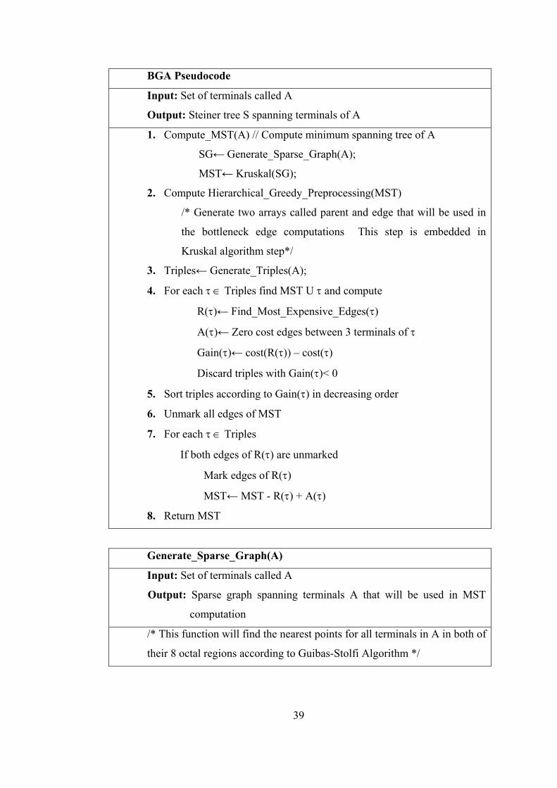
39

BGA Pseudocode

Input: Set of terminals called A

Output: Steiner tree S spanning terminals of A

1. Compute_MST(A) // Compute minimum spanning tree of A

SG← Generate_Sparse_Graph(A);

MST← Kruskal(SG);

2. Compute Hierarchical_Greedy_Preprocessing(MST)

/* Generate two arrays called parent and edge that will be used in

the bottleneck edge computations This step is embedded in

Kruskal algorithm step*/

3. Triples← Generate_Triples(A);

4. For each τ ∈ Triples find MST U τ and compute

R(τ)← Find_Most_Expensive_Edges(τ)

A(τ)← Zero cost edges between 3 terminals of τ

Gain(τ)← cost(R(τ)) – cost(τ)

Discard triples with Gain(τ)< 0

5. Sort triples according to Gain(τ) in decreasing order

6. Unmark all edges of MST

7. For each τ ∈ Triples

If both edges of R(τ) are unmarked

Mark edges of R(τ)

MST← MST - R(τ) + A(τ)

8. Return MST

Generate_Sparse_Graph(A)


Output: Sparse graph spanning terminals A that will be used in MST

computation

/* This function will find the nearest points for all terminals in A in both of

their 8 octal regions according to Guibas-Stolfi Algorithm */

40

1. For i=1 to 4 // first 4 octants

transformed← Transform the terminals ∈ octant(i) to first quadrant

Sort points according to x coordinates in ascending order

edges← Find_NE_SW_Nearest_Neighbors(transformed)

2. Return edges

Find_NE_SW_Nearest_Neighbors(transformed)

While transformed has more than 2 elements do

Find_NE_Nearest_Neighbors(1st half of transformed)

Find_NE_Nearest_Neighbors(2nd half of transformed)

Merge(1st half of transformed,2nd half of transformed)

// y-sorted list will also be calculated in parallel

Edges← Nearest_NE[transformed], Nearest_SW[transformed]

Merge(1st half of transformed,2nd half of transformed)

left← Biggest y coordinate in the 1st half

right← Biggest y coordinate in the 2nd half

min← Biggest y coordinate in the 2nd half

while( y[left]> y[right]) do

left← advance next point in the 1st half in decreasing y

while there are unprocessed elements in the 1st half do

while(y[right]> y[left]) do

if (||left,right||< ||left,min||) /* distances are calculated in

L1 distances */

min← right

right← advance next point in the 2nd half

Nearest_NE[left] ← min

Repeat same procedure for South-West region also

Kruskal (SG)

Input: Set of terminals A and sparse graph SG

Output: Minimum spanning tree spanning of A

1. MST← 0

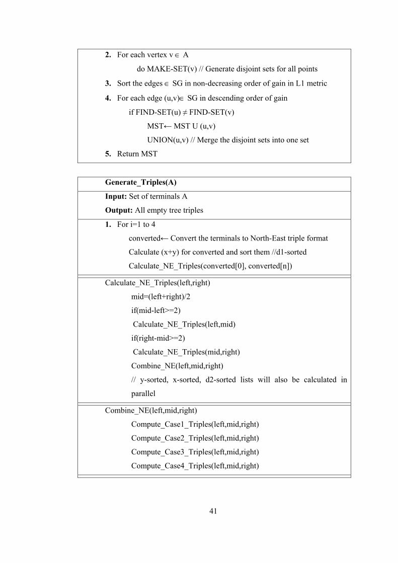
41

2. For each vertex v ∈ A

do MAKE-SET(v) // Generate disjoint sets for all points

3. Sort the edges ∈ SG in non-decreasing order of gain in L1 metric

4. For each edge (u,v)∈ SG in descending order of gain

if FIND-SET(u) ≠ FIND-SET(v)

MST← MST U (u,v)

UNION(u,v) // Merge the disjoint sets into one set

5. Return MST

Generate_Triples(A)

Input: Set of terminals A

Output: All empty tree triples

1. For i=1 to 4

converted← Convert the terminals to North-East triple format

Calculate (x+y) for converted and sort them //d1-sorted

Calculate_NE_Triples(converted[0], converted[n])

Calculate_NE_Triples(left,right)

mid=(left+right)/2

if(mid-left>=2)

Calculate_NE_Triples(left,mid)

if(right-mid>=2)

Calculate_NE_Triples(mid,right)

Combine_NE(left,mid,right)

// y-sorted, x-sorted, d2-sorted lists will also be calculated in

parallel

Combine_NE(left,mid,right)

Compute_Case1_Triples(left,mid,right)




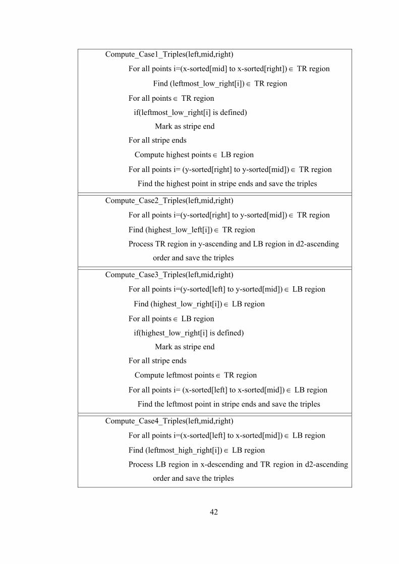
42


For all points i=(x-sorted[mid] to x-sorted[right]) ∈ TR region

Find (leftmost_low_right[i]) ∈ TR region

For all points ∈ TR region

if(leftmost_low_right[i] is defined)

Mark as stripe end

For all stripe ends

Compute highest points ∈ LB region

For all points i= (y-sorted[right] to y-sorted[mid]) ∈ TR region

Find the highest point in stripe ends and save the triples


For all points i=(y-sorted[right] to y-sorted[mid]) ∈ TR region

Find (highest_low_left[i]) ∈ TR region

Process TR region in y-ascending and LB region in d2-ascending

order and save the triples


For all points i=(y-sorted[left] to y-sorted[mid]) ∈ LB region

Find (highest_low_right[i]) ∈ LB region

For all points ∈ LB region

if(highest_low_right[i] is defined)

Mark as stripe end

For all stripe ends

Compute leftmost points ∈ TR region

For all points i= (x-sorted[left] to x-sorted[mid]) ∈ LB region

Find the leftmost point in stripe ends and save the triples


For all points i=(x-sorted[left] to x-sorted[mid]) ∈ LB region

Find (leftmost_high_right[i]) ∈ LB region

Process LB region in x-descending and TR region in d2-ascending

order and save the triples

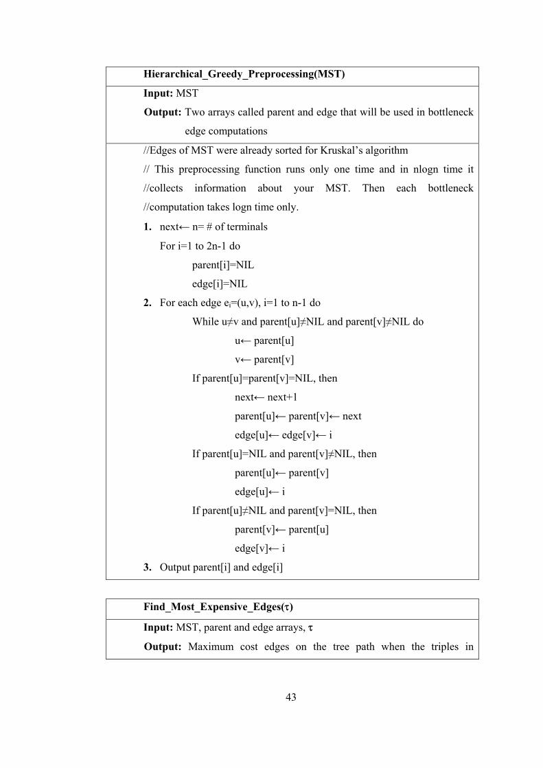
43

Hierarchical_Greedy_Preprocessing(MST)

Input: MST

Output: Two arrays called parent and edge that will be used in bottleneck

edge computations

//Edges of MST were already sorted for Kruskal’s algorithm

// This preprocessing function runs only one time and in nlogn time it

//collects information about your MST. Then each bottleneck

//computation takes logn time only.

1. next← n= # of terminals

For i=1 to 2n-1 do

parent[i]=NIL

edge[i]=NIL

2. For each edge ei=(u,v), i=1 to n-1 do

While u≠v and parent[u]≠NIL and parent[v]≠NIL do

u← parent[u]

v← parent[v]

If parent[u]=parent[v]=NIL, then

next← next+1

parent[u]← parent[v]← next

edge[u]← edge[v]← i

If parent[u]=NIL and parent[v]≠NIL, then

parent[u]← parent[v]

edge[u]← i

If parent[u]≠NIL and parent[v]=NIL, then

parent[v]← parent[u]

edge[v]← i

3. Output parent[i] and edge[i]

Find_Most_Expensive_Edges(τ)

Input: MST, parent and edge arrays, τ

Output: Maximum cost edges on the tree path when the triples in

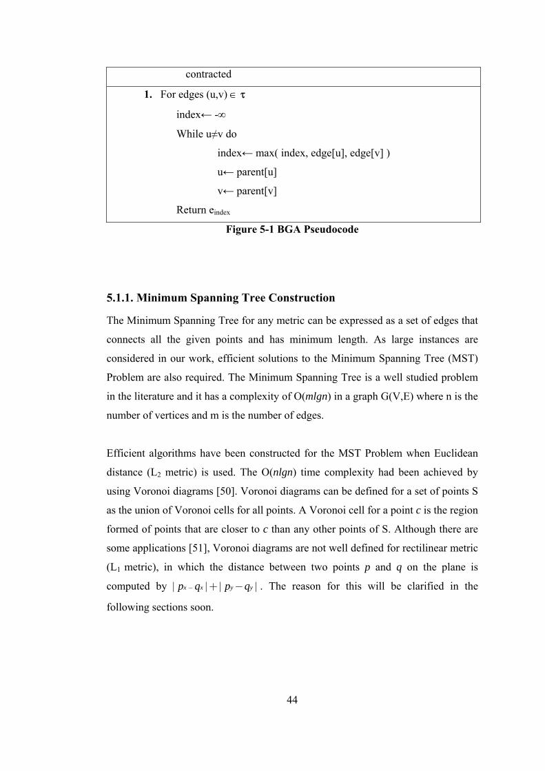
44

contracted

1. For edges (u,v) ∈ τ

index← -∞

While u≠v do

index← max( index, edge[u], edge[v] )

u← parent[u]

v← parent[v]

Return eindex

Figure 5-1 BGA Pseudocode

5.1.1. Minimum Spanning Tree Construction

The Minimum Spanning Tree for any metric can be expressed as a set of edges that

connects all the given points and has minimum length. As large instances are

considered in our work, efficient solutions to the Minimum Spanning Tree (MST)

Problem are also required. The Minimum Spanning Tree is a well studied problem

in the literature and it has a complexity of O(mlgn) in a graph G(V,E) where n is the

number of vertices and m is the number of edges.

Efficient algorithms have been constructed for the MST Problem when Euclidean

distance (L2 metric) is used. The O(nlgn) time complexity had been achieved by

using Voronoi diagrams [50]. Voronoi diagrams can be defined for a set of points S

as the union of Voronoi cells for all points. A Voronoi cell for a point c is the region

formed of points that are closer to c than any other points of S. Although there are

some applications [51], Voronoi diagrams are not well defined for rectilinear metric

(L1 metric), in which the distance between two points p and q on the plane is

computed by | | | |x x y yp q p q− + − . The reason for this will be clarified in the

following sections soon.

45

Because of the problem that exists in the computation of the spanning tree directly

in the L1 metric, other methods have been proposed. The most efficient one that has

been built is the sparse spanning graph concept. The main idea behind this method

is to find efficiently first a sparse graph that contains the MST and then to work on

this graph afterwards.

5.1.1.1. Sparse Spanning Graphs

In order to find the Minimum Spanning Tree for L1 metric, first a spanning graph

for the set of points is constructed. Input to the proposed algorithms to find the

spanning graphs is the set of points, call V. The spanning graph G= (V,E) is called a

spanning graph if it contains a minimum spanning tree of the complete graph. The

cost of the edges E are all computed in L1 metric. It is trivial that complete graph

which have n*(n-1) edges where n is equal to the number of elements of V, has the

MST inside it. Actually what is needed are sparse graphs that include MST inside.

The least dense graph obtainable that includes MST is the MST itself. So there must

be a trade off between a complete graph, which is easy to implement but so

crowded and MST, which is sparse but hard to implement.

The main idea in the sparse graph construction is to eliminate edges that are

guaranteed not to exist in the MST and to include edges that are guaranteed to exist

in the MST. The first property is the cut property. This property says that an edge of

smallest weight crossing any partition of the vertex set V into two parts belong to

MST. The second property is the cycle property, which states that an edge with

largest weight in any formed cycle in the graph can be safely deleted.

In [52] it is shown that for any partition of V, say V1 and V2 if |qp| is the shortest

segment between V1 and V2 then q is in the Voronoi diagram of V. By considering

strong cut property a Voronoi diagram can be used as a spanning graph in L2 metric.

But in the L1 metric consider the case where half of the points of V take place in the

x+y=c segment and half of them in the x-y=c segment. Then all edges between these

46

two subsets have the same length and all must be included in the spanning graph

according to the strong cut property.

According to the above results, new methodologies have been constructed for

spanning graph construction in L1 metric. In BGA, Guibas-Stolfi algorithm is used

for the sparse graph computation [53]. In RST, a Rectilinear Spanning Graph is

constructed for the same purpose and it will be explained in detail later. Both of

these algorithms uses octal partitioning concept. In the next section octal

partitioning and its use in sparse spanning graph computation is explained and

afterwards Guibas-Stolfi’s algorithm will be defined in the following section.

5.1.1.2. Use of Octal Partitions in Spanning Graph Computation

In order to explain the octal partitioning phenomena, first strict uniqueness property

needs to be defined.

Strict Uniqueness Property: Given a point p, a region R has the strict uniqueness

property with respect to p, if for every pair of points u, w ∈ R either

( , ) ( , )dist w u dist w p< or ( , ) ( , )dist u w dist u p< . A partition of space into a finite set

of disjoint regions is said to have the strict uniqueness property if each of its regions

have the strict uniqueness property [54].

There are different partition schemes that the strict uniqueness property can be

satisfied. But now octal partitioning will be defined and how it can be used for

spanning graph computations will be shown. Define the octal partition for point p as

two rectilinear lines and two 45 degree lines as can be seen in Figure 5-2(a). The

regions in the figure involve the line to the left of the region in, as illustrated in

Figure 5-2(b).

47

Figure 5-2 Octal Partitions for a point p

Now it must be proved that the octal partitioning have the strict uniqueness property.

For this, all regions from R1 to R8 must have strict uniqueness property. Since they

are similar, only R1 region will be shown to have the uniqueness property. All

others can then be shown to have it.

For the point p, the points (x, y) ∈ R1 region have the following inequalities:

p

p p

x xx y x y≥− < −

(5.1)

Now let us assume that we have two points u and w in R1 region. And also assume

that u wx x≤ . If u wy y≤ , then we have automatically pw pu uw uw= + >

where ab represents the rectilinear distance between point a and b. And for

u wy y> we have

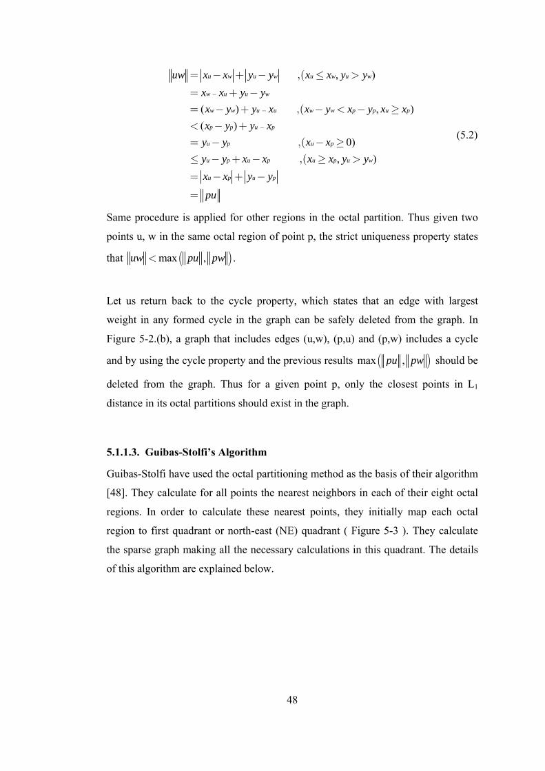
48

, )

( ) , )( )

0), )

u w u w u w u w

w u u w

w w u u w w p p u p

p p u p

u p u p

u p u p u p u w

u p

uw x x y y x x y yx x y yx y y x x y x y x xx y y x

y y x xy y x x x x y yx x y

−

−

−

= − + − ,( ≤ >= + − = − + ,( − < − ≥< − += − ,( − ≥≤ − + − ,( ≥ >= − + u py

pu

−

=

(5.2)

Same procedure is applied for other regions in the octal partition. Thus given two

points u, w in the same octal region of point p, the strict uniqueness property states

that ( )max ,uw pu pw< .

Let us return back to the cycle property, which states that an edge with largest

weight in any formed cycle in the graph can be safely deleted from the graph. In

Figure 5-2.(b), a graph that includes edges (u,w), (p,u) and (p,w) includes a cycle

and by using the cycle property and the previous results ( )max ,pu pw should be

deleted from the graph. Thus for a given point p, only the closest points in L1

distance in its octal partitions should exist in the graph.

5.1.1.3. Guibas-Stolfi’s Algorithm

Guibas-Stolfi have used the octal partitioning method as the basis of their algorithm

[48]. They calculate for all points the nearest neighbors in each of their eight octal

regions. In order to calculate these nearest points, they initially map each octal

region to first quadrant or north-east (NE) quadrant ( Figure 5-3 ). They calculate

the sparse graph making all the necessary calculations in this quadrant. The details

of this algorithm are explained below.

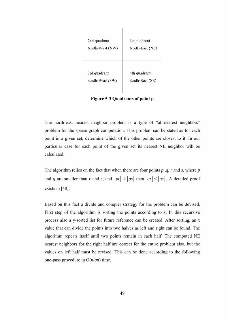
49

Figure 5-3 Quadrants of point p

The north-east nearest neighbor problem is a type of “all-nearest neighbors”

problem for the sparse graph computation. This problem can be stated as for each

point in a given set, determine which of the other points are closest to it. In our

particular case for each point of the given set its nearest NE neighbor will be

calculated.

The algorithm relies on the fact that when there are four points p ,q, r and s, where p

and q are smaller than r and s, and pr ps≤ then qr qs≤ . A detailed proof

exists in [48].

Based on this fact a divide and conquer strategy for the problem can be devised.

First step of the algorithm is sorting the points according to x. In this recursive

process also a y-sorted list for future reference can be created. After sorting, an x

value that can divide the points into two halves as left and right can be found. The

algorithm repeats itself until two points remain in each half. The computed NE

nearest neighbors for the right half are correct for the entire problem also, but the

values on left half must be revised. This can be done according to the following

one-pass procedure in O(nlgn) time.

50

There will be three pointers used for this computation. Pointer left will advance

down the y-sorted list for the left half starting from the biggest y-element. As it is

mentioned above y-sorted list will be formed in the algorithm during recursion

process. The purpose of this algorithm is to compute the NE nearest neighbor for

the pointer left. Pointer right and min will advance down the y-sorted list for the

right half starting from the biggest y-element. Pointer right must always be higher

than left, so it will be revised to be bigger than left in the beginning of the algorithm.

Pointer min is used to keep track of the nearest right half element for left seen until

now.

Now for any left value that the NE nearest neighbor is being sought the procedure is

started by finding the right element in the right half. Also set this element as min

because it is the nearest point to left seen until now. Then advance right in the right

hand plane as follows:

- If the point that right shows is higher than left in y, but the rectilinear

distance between right and left is larger than the rectilinear distance between

min and left, then advance right again

- If the point that right shows is higher than left in y, and the rectilinear

distance between right and left is smaller than the rectilinear distance

between min and left, then set min equal to right and advance right again

- If the point that right shows drops below the left in y, then set min as the

nearest NE neighbor of left, and advance left.

Actually by applying this recursive procedure all nearest NE neighbors can be

computed for a set of points. By the same procedure also the nearest SW neighbors

can be calculated in parallel in order to reduce the computation time.

But the algorithm is not finished yet. We have to find the nearest NE neighbors for

all points but what we need actually is to find the nearest octal neighbors of all

points. This is done by making transformations of all octants into first quadrant.

When making transformations some information about the points has to be

protected.

51

- If q is in the kth octant of p, then Tq must be in the first quadrant of Tp.

- If q1 and q2 are two points in the kth octant of p, and 1 2pq pq≤ , then

1 2p q p qT T T T≤ .

where Ti represents the transformed point of i into first quadrant. Now the transfer

functions for the octal regions will be calculated.

For octal region 1 which can be seen in Figure 5-4 the transformed function T can

be ( ) ( ): , 2 ,T x y x y x→ − . This function will map octal region 1 to first quadrant

which can be seen in Figure 5-5. Also the properties that the transformation has to

satisfy are proved below.

Figure 5-4 Octal Region 1

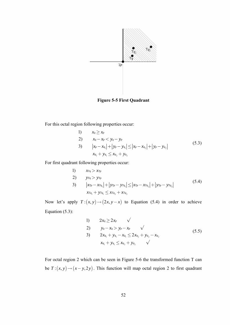
52

Figure 5-5 First Quadrant

For this octal region following properties occur:

1 1 2 2

1 1 2 2

1)2)3)

q p

q p q p

p q p q p q p q

q q q q

x xx x y yx x y y x x y yx y x y

≥ − < −

− + − ≤ − + − + ≤ +

(5.3)

For first quadrant following properties occur:

1 1 2 2

1 1 2 2

1)2)3)

Tq Tp

Tq Tp

Tp Tq Tp Tq Tp Tq Tp Tq

Tq Tq Tq Tq

x xy yx x y y x x y yx y x x

> >

− + − ≤ − + − + ≤ +

(5.4)

Now let’s apply ( ) ( ): , 2 ,T x y x y x→ − to Equation (5.4) in order to achieve

Equation (5.3):

1 1 1 2 2 2

1 1 2 2

1) 2

2)3) 2

q p

q q p p

q q q q q q

q q q q

x x

y x y xx y x x y x

x y x y

2 ≥ √ − > − √

2 + − ≤ + − + ≤ + √

(5.5)


be ( ) ( ): , , 2T x y x y y→ − . This function will map octal region 2 to first quadrant

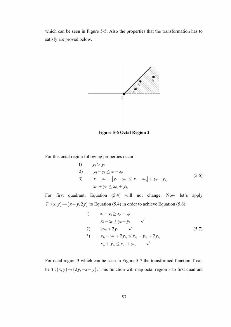
53





1 1 2 2

1 1 2 2

1)2)3)

q p

q p q p

p q p q p q p q

q q q q

y yy y x xx x y y x x y yx y x y

> − ≤ −

− + − ≤ − + − + ≤ +

(5.6)

For first quadrant, Equation (5.4) will not change. Now let’s apply

( ) ( ): , , 2T x y x y y→ − to Equation (5.4) in order to achieve Equation (5.6):

1 1 1 2 2 2

1 1 2 2

1)

2) 23) 2 2

q q p p

q p q p

q p

q q q q q q

q q q q

x y x y

x x y y

y yx y y x y y

x y x y

− ≥ − − ≥ − √

2 > √ − + ≤ − +

+ ≤ + √

(5.7)


be ( ) ( ): , 2 ,T x y y x y→ − − . This function will map octal region 3 to first quadrant

54





1 1 2 2

1 1 2 2

1)2)3)

q p

q q p p

p q p q p q p q

q q q q

y yx y x yx x y y x x y yy x y x

> + ≤ +

− + − ≤ − + − − ≤ −

(5.8)


( ) ( ): , 2 ,T x y y x y→ − − to Equation (5.4) in order to achieve Equation (5.8):

1 1 1 2 2 2

1 1 2 2

1) 22)

3) 2 2

q p

q q p p

q q p p

q q q q q q

q q q q

y yx y x y

x y x yy x y y x y

y x y x

2 ≥ √ − − >− −

+ < + √ − − ≤ − −

− ≤ − √

(5.9)


be ( ) ( ): , , 2T x y x y x→ + − . This function will map octal region 4 to first quadrant

55





1 1 2 2

1 1 2 2

1)2)3)

q p

q q p p

p q p q p q p q

q q q q

x yx y x yx x y y x x y yy x y x

< + ≥ +

− + − ≤ − + − − ≤ −

(5.10)


( ) ( ): , , 2T x y x y x→ + − to Equation (5.4) in order to achieve Equation (5.10):

1 1 1 2 2 2

1 1 2 2

1)2) 2

3) 2 2

q q p p

q p

q p

q q q q q q

q q q q

x y x yx x

x xx y x x y x

y x y x

+ ≥ + √ −2 >−

< √ + − ≤ + −

− ≤ − √

(5.11)

As a result, following the application of the specified algorithm above, all points in

the given set are connected to all nearest neighbors in their octal partition as in the

following figure:

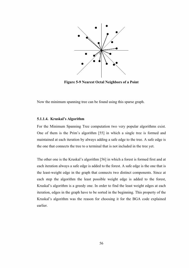
56

Figure 5-9 Nearest Octal Neighbors of a Point

Now the minimum spanning tree can be found using this sparse graph.

5.1.1.4. Kruskal’s Algorithm

For the Minimum Spanning Tree computation two very popular algorithms exist.

One of them is the Prim’s algorithm [55] in which a single tree is formed and

maintained at each iteration by always adding a safe edge to the tree. A safe edge is

the one that connects the tree to a terminal that is not included in the tree yet.

The other one is the Kruskal’s algorithm [56] in which a forest is formed first and at

each iteration always a safe edge is added to the forest. A safe edge is the one that is

the least-weight edge in the graph that connects two distinct components. Since at

each step the algorithm the least possible weight edge is added to the forest,

Kruskal’s algorithm is a greedy one. In order to find the least weight edges at each

iteration, edges in the graph have to be sorted in the beginning. This property of the

Kruskal’s algorithm was the reason for choosing it for the BGA code explained

earlier.

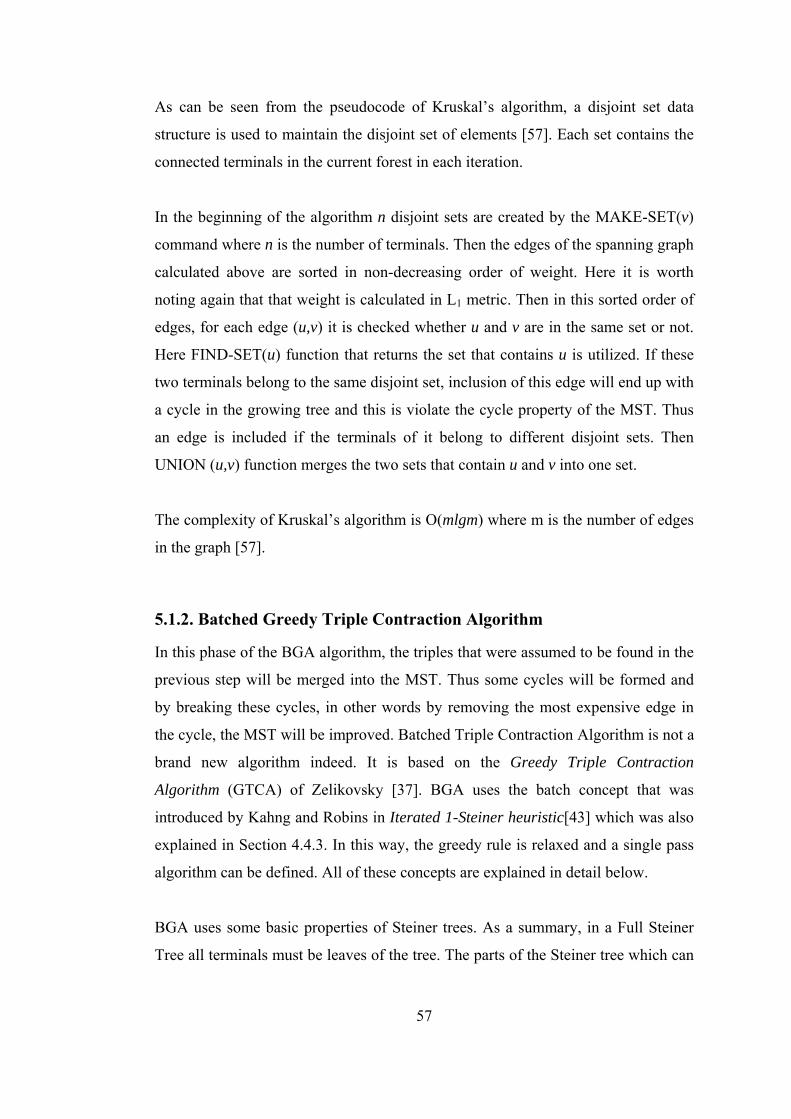
57

As can be seen from the pseudocode of Kruskal’s algorithm, a disjoint set data

structure is used to maintain the disjoint set of elements [57]. Each set contains the

connected terminals in the current forest in each iteration.

In the beginning of the algorithm n disjoint sets are created by the MAKE-SET(v)

command where n is the number of terminals. Then the edges of the spanning graph

calculated above are sorted in non-decreasing order of weight. Here it is worth

noting again that that weight is calculated in L1 metric. Then in this sorted order of

edges, for each edge (u,v) it is checked whether u and v are in the same set or not.

Here FIND-SET(u) function that returns the set that contains u is utilized. If these

two terminals belong to the same disjoint set, inclusion of this edge will end up with

a cycle in the growing tree and this is violate the cycle property of the MST. Thus

an edge is included if the terminals of it belong to different disjoint sets. Then

UNION (u,v) function merges the two sets that contain u and v into one set.

The complexity of Kruskal’s algorithm is O(mlgm) where m is the number of edges

in the graph [57].

5.1.2. Batched Greedy Triple Contraction Algorithm

In this phase of the BGA algorithm, the triples that were assumed to be found in the

previous step will be merged into the MST. Thus some cycles will be formed and

by breaking these cycles, in other words by removing the most expensive edge in

the cycle, the MST will be improved. Batched Triple Contraction Algorithm is not a

brand new algorithm indeed. It is based on the Greedy Triple Contraction

Algorithm (GTCA) of Zelikovsky [37]. BGA uses the batch concept that was

introduced by Kahng and Robins in Iterated 1-Steiner heuristic[43] which was also

explained in Section 4.4.3. In this way, the greedy rule is relaxed and a single pass

algorithm can be defined. All of these concepts are explained in detail below.

BGA uses some basic properties of Steiner trees. As a summary, in a Full Steiner

Tree all terminals must be leaves of the tree. The parts of the Steiner tree which can

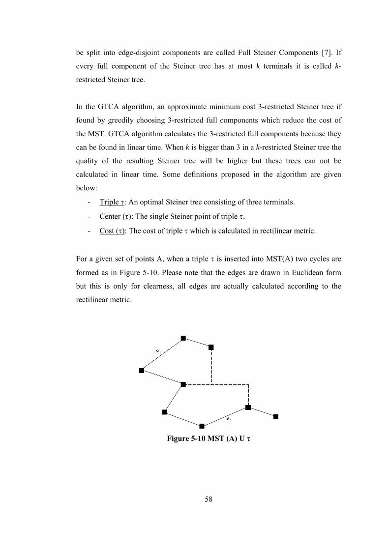
58

be split into edge-disjoint components are called Full Steiner Components [7]. If

every full component of the Steiner tree has at most k terminals it is called k-

restricted Steiner tree.

In the GTCA algorithm, an approximate minimum cost 3-restricted Steiner tree if

found by greedily choosing 3-restricted full components which reduce the cost of

the MST. GTCA algorithm calculates the 3-restricted full components because they

can be found in linear time. When k is bigger than 3 in a k-restricted Steiner tree the

quality of the resulting Steiner tree will be higher but these trees can not be

calculated in linear time. Some definitions proposed in the algorithm are given

below:

- Triple τ: An optimal Steiner tree consisting of three terminals.

- Center (τ): The single Steiner point of triple τ.

- Cost (τ): The cost of triple τ which is calculated in rectilinear metric.

For a given set of points A, when a triple τ is inserted into MST(A) two cycles are

formed as in Figure 5-10. Please note that the edges are drawn in Euclidean form

but this is only for clearness, all edges are actually calculated according to the

rectilinear metric.

Figure 5-10 MST (A) U τ

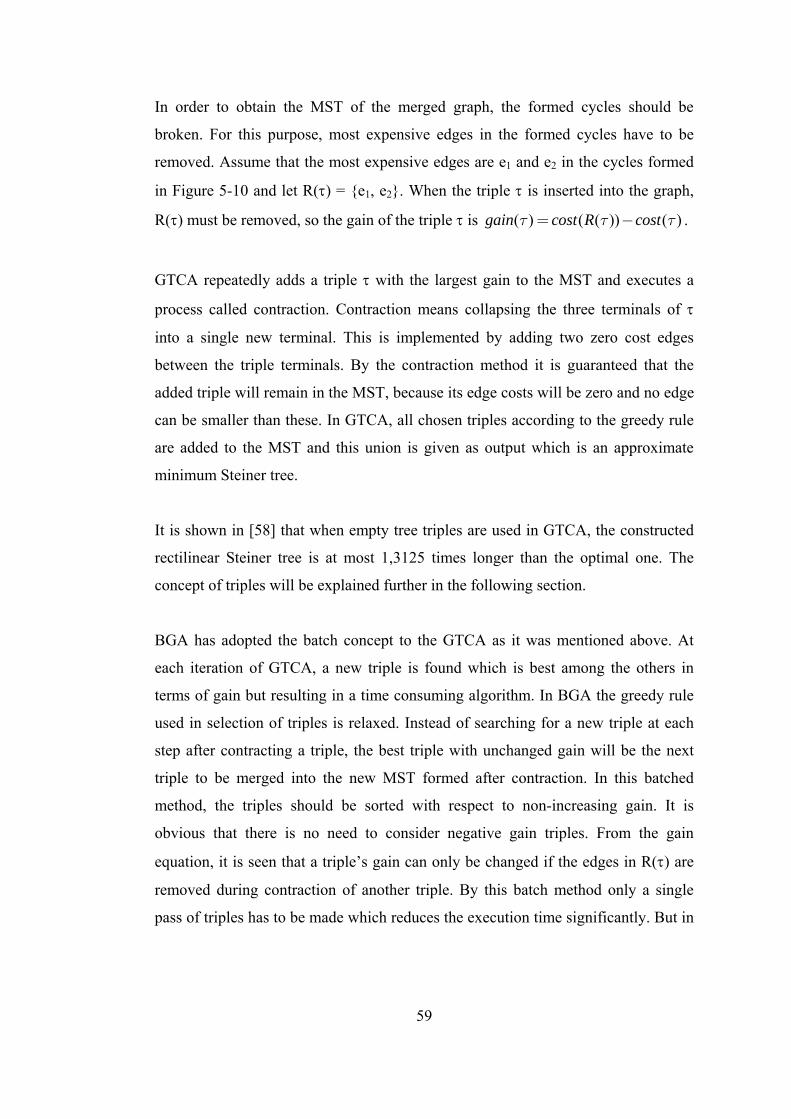
59

In order to obtain the MST of the merged graph, the formed cycles should be

broken. For this purpose, most expensive edges in the formed cycles have to be

removed. Assume that the most expensive edges are e1 and e2 in the cycles formed

in Figure 5-10 and let R(τ) = {e1, e2}. When the triple τ is inserted into the graph,

R(τ) must be removed, so the gain of the triple τ is ( ) ( ( )) ( )gain cost R costτ τ τ= − .

GTCA repeatedly adds a triple τ with the largest gain to the MST and executes a

process called contraction. Contraction means collapsing the three terminals of τ

into a single new terminal. This is implemented by adding two zero cost edges

between the triple terminals. By the contraction method it is guaranteed that the

added triple will remain in the MST, because its edge costs will be zero and no edge

can be smaller than these. In GTCA, all chosen triples according to the greedy rule

are added to the MST and this union is given as output which is an approximate

minimum Steiner tree.

It is shown in [58] that when empty tree triples are used in GTCA, the constructed

rectilinear Steiner tree is at most 1,3125 times longer than the optimal one. The

concept of triples will be explained further in the following section.

BGA has adopted the batch concept to the GTCA as it was mentioned above. At

each iteration of GTCA, a new triple is found which is best among the others in

terms of gain but resulting in a time consuming algorithm. In BGA the greedy rule

used in selection of triples is relaxed. Instead of searching for a new triple at each

step after contracting a triple, the best triple with unchanged gain will be the next

triple to be merged into the new MST formed after contraction. In this batched

method, the triples should be sorted with respect to non-increasing gain. It is

obvious that there is no need to consider negative gain triples. From the gain

equation, it is seen that a triple’s gain can only be changed if the edges in R(τ) are

removed during contraction of another triple. By this batch method only a single

pass of triples has to be made which reduces the execution time significantly. But in

60

the batched method triples that have positive gain may still remain. More than a

single pass of algorithm can be run in order to include them also.

5.1.3. Generation of Triples

The empty tree triples are used to shorten the MST. All empty tree triples will be

merged into the MST and the cycles formed during this process will be broken

which may reduce the size of MST. In this part of the algorithm, all empty tree

triples will be formed for the given set of terminals. For this purpose, the triples will

be classified into 4 distinct types and these distinct types will be solved individually

in a recursive manner. Each type of these triples are divided to four distinct cases

again and they are also solved individually. First, the empty triple concept, which

was introduced in [40] will be explained and then the algorithm that calculates all

empty tree triples in O(nlgn) time will be presented.

A triple is a sub-graph that consists of three terminals. If the minimum rectangle

bounding the triple does not contain any other terminals it is called an empty triple.

If the gain obtained by merging the triple into the MST is positive it is called a tree

triple. A triple is an empty tree triple if it is an empty triple and a tree triple. It is

shown in [40] that the number of all empty tree triples are at most 36n, where n is

the number of terminals in the given set of points. In [40], all these empty tree

triples are calculated in O(n2lgn) by also maintaining dynamic minimum spanning

trees. However this approach has been shown to be very impractical for large sets of

points [59].

The triples are said to be classified to four distinct types earlier. The classification is

made according to the position of the diagonal with respect to the center where the

diagonal is the terminal of the triple which does not share the same x or y

coordinates with the center. These types are called north-west, north-east, south-

west and south-east and they are illustrated in Figure 5-11.

61

Figure 5-11 Types of triples

In order to find all these types of triples, the terminals are partitioned into almost

equal halves in a recursive manner. The lines which partition the terminals into

equal halves are changing according to the types of triples. For the north-west and

south-east types, the divisor line is parallel to line y= -x and two halves are formed

called LB (Left-Bottom) and TR (Top-Right). For the north-east and south-west

type triples, the divisor line is parallel to y= x and two halves are formed called TL

(Top-Left) and BR (Bottom-Right). All these types and divisions are illustrated in

Figure 5-12:

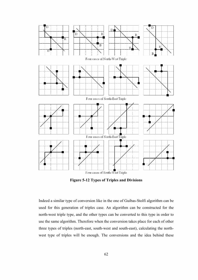
62

Figure 5-12 Types of Triples and Divisions

Indeed a similar type of conversion like in the one of Guibas-Stolfi algorithm can be

used for this generation of triples case. An algorithm can be constructed for the

north-west triple type, and the other types can be converted to this type in order to

use the same algorithm. Therefore when the conversion takes place for each of other

three types of triples (north-east, south-west and south-east), calculating the north-

west type of triples will be enough. The conversions and the idea behind these

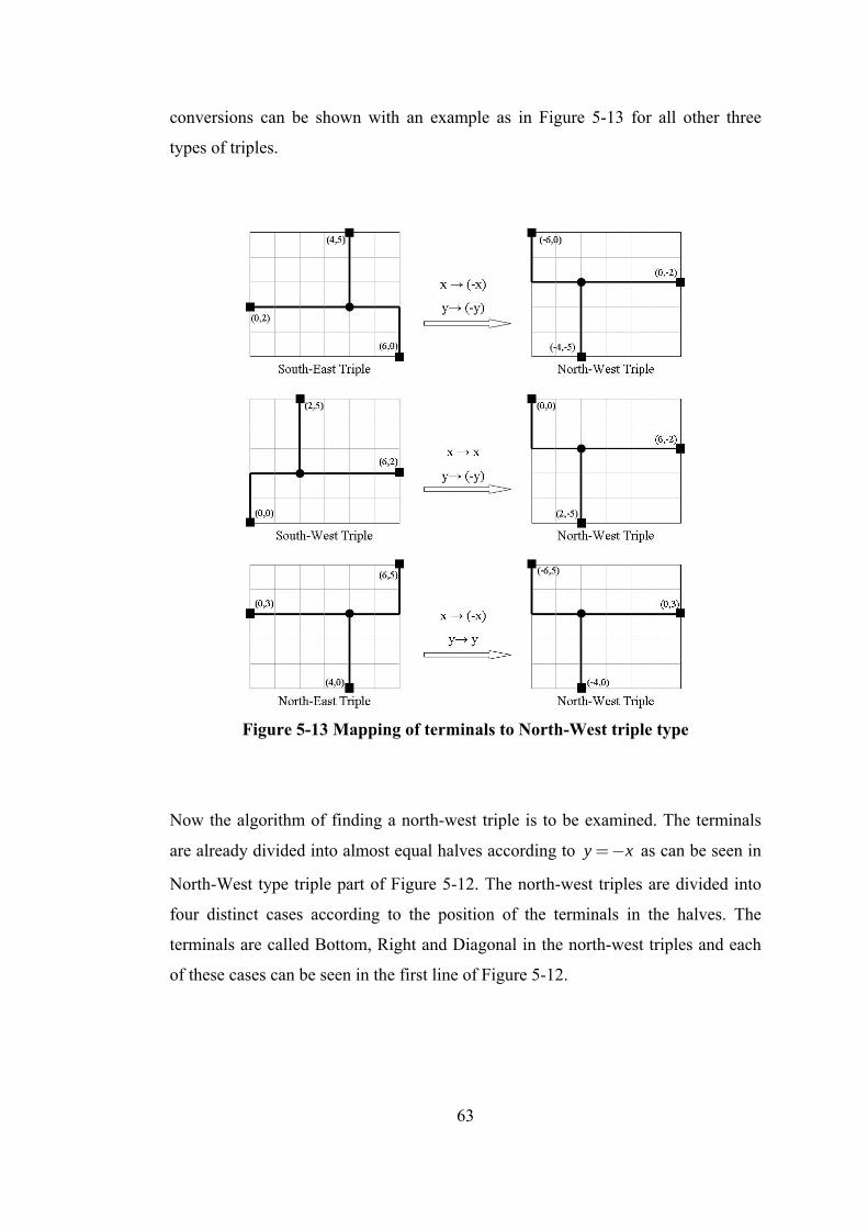
63

conversions can be shown with an example as in Figure 5-13 for all other three

types of triples.

Figure 5-13 Mapping of terminals to North-West triple type

Now the algorithm of finding a north-west triple is to be examined. The terminals

are already divided into almost equal halves according to y x=− as can be seen in

North-West type triple part of Figure 5-12. The north-west triples are divided into

four distinct cases according to the position of the terminals in the halves. The

terminals are called Bottom, Right and Diagonal in the north-west triples and each

of these cases can be seen in the first line of Figure 5-12.

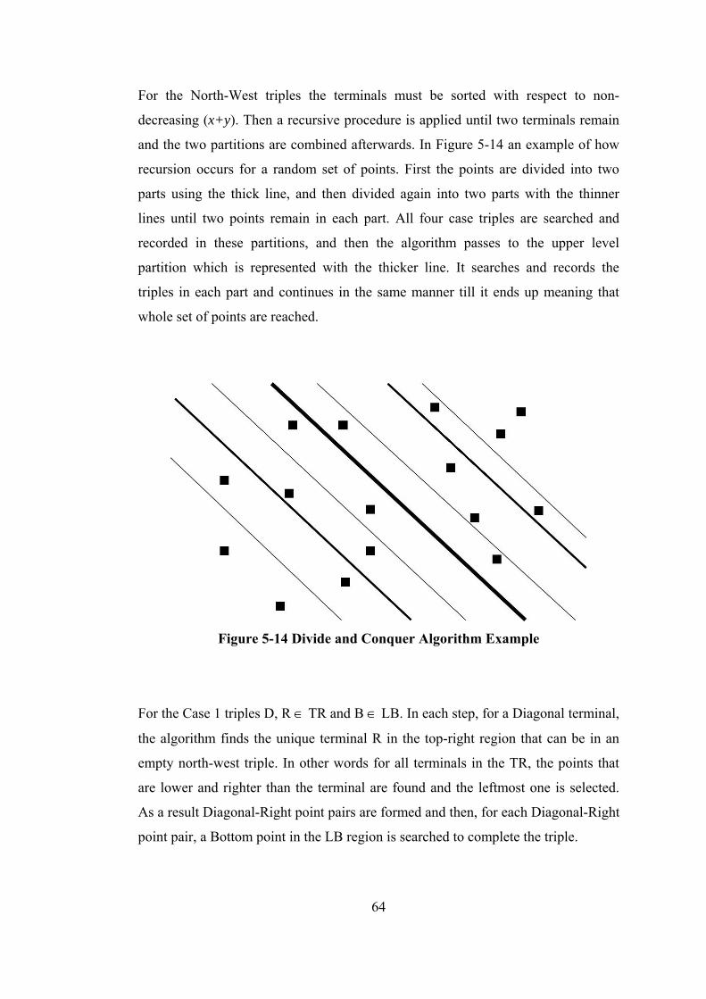
64

For the North-West triples the terminals must be sorted with respect to non-

decreasing (x+y). Then a recursive procedure is applied until two terminals remain

and the two partitions are combined afterwards. In Figure 5-14 an example of how

recursion occurs for a random set of points. First the points are divided into two

parts using the thick line, and then divided again into two parts with the thinner

lines until two points remain in each part. All four case triples are searched and

recorded in these partitions, and then the algorithm passes to the upper level

partition which is represented with the thicker line. It searches and records the

triples in each part and continues in the same manner till it ends up meaning that

whole set of points are reached.

Figure 5-14 Divide and Conquer Algorithm Example

For the Case 1 triples D, R ∈ TR and B ∈ LB. In each step, for a Diagonal terminal,

the algorithm finds the unique terminal R in the top-right region that can be in an

empty north-west triple. In other words for all terminals in the TR, the points that

are lower and righter than the terminal are found and the leftmost one is selected.

As a result Diagonal-Right point pairs are formed and then, for each Diagonal-Right

point pair, a Bottom point in the LB region is searched to complete the triple.

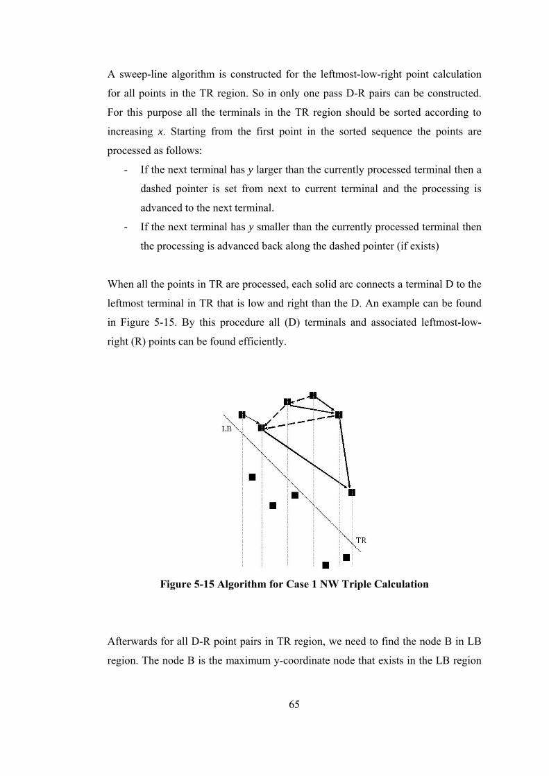
65

A sweep-line algorithm is constructed for the leftmost-low-right point calculation

for all points in the TR region. So in only one pass D-R pairs can be constructed.

For this purpose all the terminals in the TR region should be sorted according to

increasing x. Starting from the first point in the sorted sequence the points are

processed as follows:

- If the next terminal has y larger than the currently processed terminal then a

dashed pointer is set from next to current terminal and the processing is

advanced to the next terminal.

- If the next terminal has y smaller than the currently processed terminal then

the processing is advanced back along the dashed pointer (if exists)

When all the points in TR are processed, each solid arc connects a terminal D to the

leftmost terminal in TR that is low and right than the D. An example can be found

in Figure 5-15. By this procedure all (D) terminals and associated leftmost-low-

right (R) points can be found efficiently.

Figure 5-15 Algorithm for Case 1 NW Triple Calculation

Afterwards for all D-R point pairs in TR region, we need to find the node B in LB

region. The node B is the maximum y-coordinate node that exists in the LB region

66

and in the vertical strip defined by D and R. This can also be done in a sweeping

manner. First the stripe ends are marked and in ascending x order in LB the upper

point in these stripe ends are computed. Then starting from the highest point in TR

region, where we have the points in y-sorted order, all Bottom points are computed

in order to complete the triples. In each recursion step, the calculated triples are

saved and the recursion goes on. Therefore, the triples are not forming only in the

last step.

For the Case 2 triples B, R ∈ TR and D ∈ LB. In each step, for a Right terminal, the

recursive algorithm computes the unique terminal Bottom in the top-right region

that can be in an empty north-west triple. This time, for all terminals in TR, the

highest-low-left point is calculated that is in TR also. This can be made by a similar

procedure that is explained above in the Case 1 triples. This time the points in the

TR region must be sorted in non-increasing order for the sweeping process. Then in

the formed Right-Bottom point pairs Diagonal points in the LB region are searched

to complete the triple.

The Diagonal point in the LB region must be the closest point to R and also to B in

order to complete the triple into an empty tree triple. Finding the D point for each

pair of R-B is a little different from the procedure defined for Case-1 triples. This

time a simultaneous traversing of terminals should be done in both TR and LB

regions. The points in the TR must be sorted in y-ascending order and LB must be

sorted in (x-y) ascending order during the traversal. The points in the TR will be

advanced until a terminal R is reached that has an arc to a B whereas the points of

LB will be advanced until a terminal higher than R is reached. Then that D is

assigned to the B-R pair as a Diagonal point of the empty NW Case 2 triple.

For Case 3 triples R ∈ TR and D, B ∈ LB. The approach is similar to the one in

Case-1. First, for all points in LB, a point that will serve as a Bottom point is found.

This is equivalent to finding a point that is the highest low-right point of the

currently processed point. This time the points in the LB must be y-sorted. For all

67

pairs D-B, R points are required to be calculated in the LB region. After the similar

sweeping algorithm is used for the D-B pair computation, the stripe ends will be

marked. Then for TR region, which is sorted according to x the leftmost points are

found and then for each D-B pair the R point that will serve in the empty Case 3

triple is found.

For Case 4 triples D ∈ TR and R, B ∈ LB. In this case, the approach is similar to

the Case 2 part. First, for all points in the LB region, associated R points will be

searched. It is the rightmost-high-left point for all pairs. Similar sweeping procedure

can be followed as in the preceding cases but the points in the LB should be x-

sorted. After R-B pairs are constructed, a D in the TR region is required to be

calculated. D will be the closest point to R and B and also D must be to the left of B.

In order to complete the triple, LB region will be advanced in x-ascending order

whereas TR region will be advanced in (x-y) ascending order.

5.1.4. Hierarchical Greedy Preprocessing Algorithm

It is shown in 5.1.2 that when a triple is merged into the MST two cycles are formed.

These cycles in the merged graph have to be broken by removing the most

expensive edges. In BGA, Hierarchical Greedy Preprocessing (HGP) algorithm is

used for this purpose. In this algorithm two arrays are formed in O(nlgn) time first

by analyzing the graph. Then each most expensive edge computation is done in

O(lgn) time. The details are explained below.

The preprocessing phase of the algorithm is very similar with the ideas of Boruvka

who has developed a method for constructing an efficient electricity network for

Bohemia, in Czech Republic, in 1926 [60]. This algorithm was also a minimum

spanning tree construction algorithm which was also applied by Sollin [61] later.

The HGP algorithm works on the edges of MST which are sorted in ascending order

of cost. Since the MST is formed by using Kruskal’s algorithm the edges are sorted

already. It has to be emphasized that this step is embedded into Kruskal

computation. As the output of the preprocessing algorithm two arrays are formed

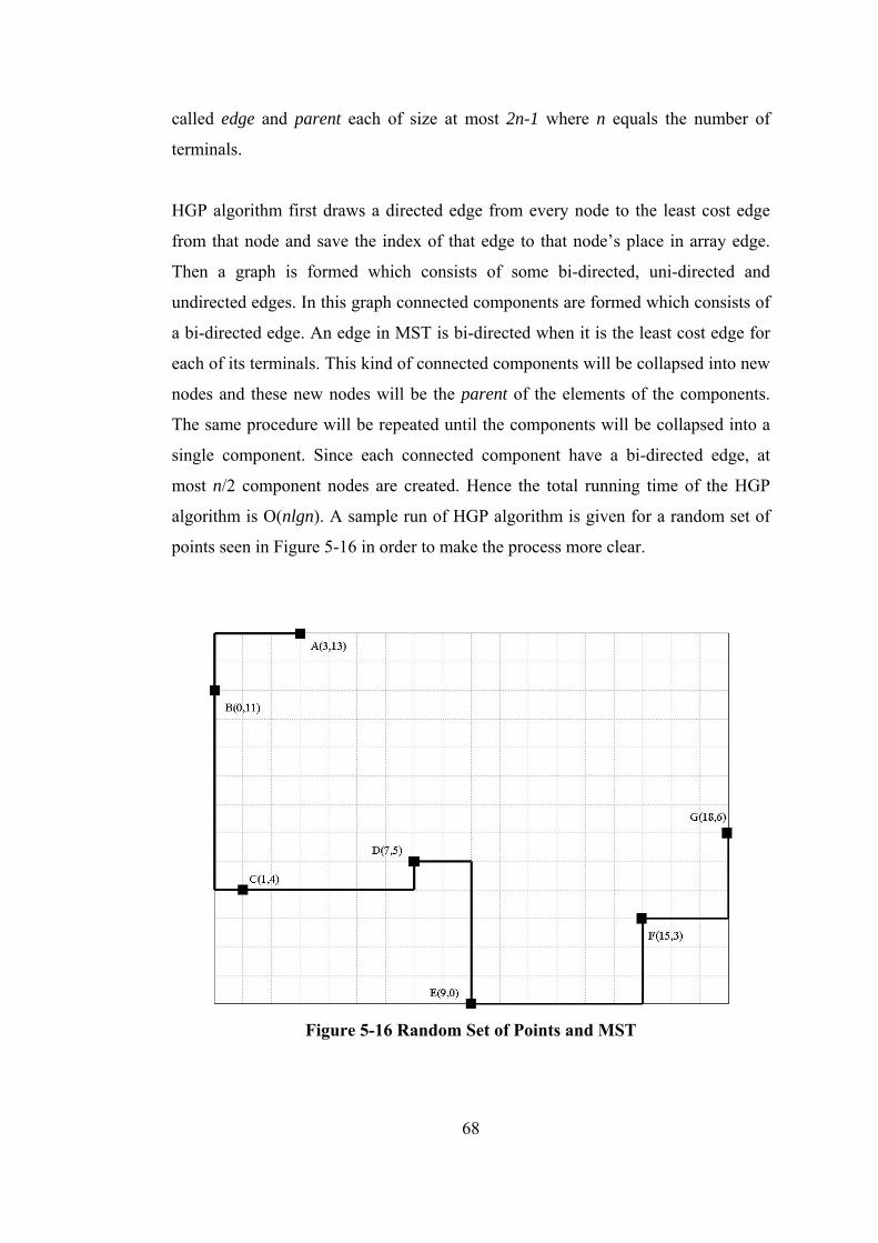
68

called edge and parent each of size at most 2n-1 where n equals the number of

terminals.

HGP algorithm first draws a directed edge from every node to the least cost edge

from that node and save the index of that edge to that node’s place in array edge.

Then a graph is formed which consists of some bi-directed, uni-directed and

undirected edges. In this graph connected components are formed which consists of

a bi-directed edge. An edge in MST is bi-directed when it is the least cost edge for

each of its terminals. This kind of connected components will be collapsed into new

nodes and these new nodes will be the parent of the elements of the components.

The same procedure will be repeated until the components will be collapsed into a

single component. Since each connected component have a bi-directed edge, at

most n/2 component nodes are created. Hence the total running time of the HGP

algorithm is O(nlgn). A sample run of HGP algorithm is given for a random set of

points seen in Figure 5-16 in order to make the process more clear.

Figure 5-16 Random Set of Points and MST

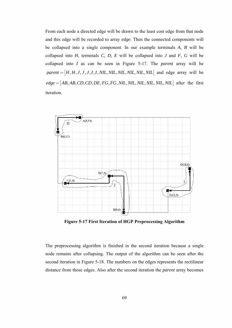
69

From each node a directed edge will be drawn to the least cost edge from that node

and this edge will be recorded to array edge. Then the connected components will

be collapsed into a single component. In our example terminals A, B will be

collapsed into H, terminals C, D, E will be collapsed into J and F, G will be

collapsed into I as can be seen in Figure 5-17. The parent array will be

[ ], , , , , , , , , , , ,parent H H J J J I I NIL NIL NIL NIL NIL NIL= and edge array will be

[ ], , , , , , , , , , , ,edge AB AB CD CD DE FG FG NIL NIL NIL NIL NIL NIL= after the first

iteration.

Figure 5-17 First Iteration of HGP Preprocessing Algorithm

The preprocessing algorithm is finished in the second iteration because a single

node remains after collapsing. The output of the algorithm can be seen after the

second iteration in Figure 5-18. The numbers on the edges represents the rectilinear

distance from those edges. Also after the second iteration the parent array becomes

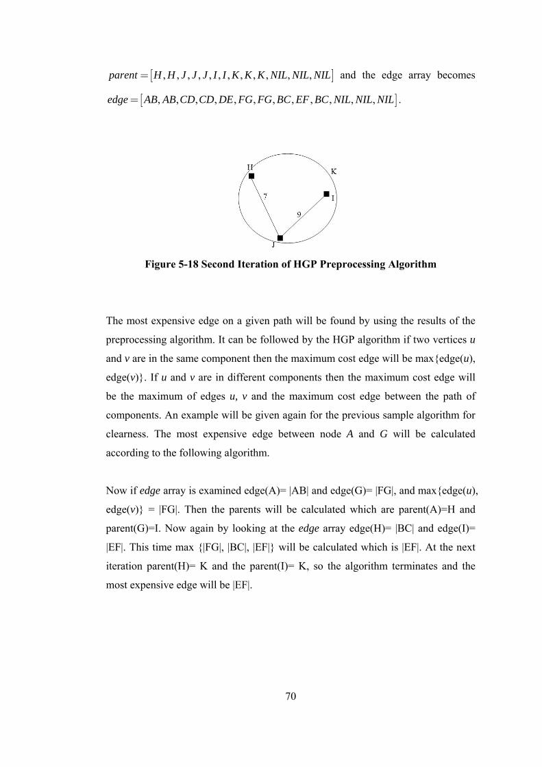
70

[ ], , , , , , , , , , , ,parent H H J J J I I K K K NIL NIL NIL= and the edge array becomes

[ ], , , , , , , , , , , ,edge AB AB CD CD DE FG FG BC EF BC NIL NIL NIL= .

Figure 5-18 Second Iteration of HGP Preprocessing Algorithm

The most expensive edge on a given path will be found by using the results of the

preprocessing algorithm. It can be followed by the HGP algorithm if two vertices u

and v are in the same component then the maximum cost edge will be max{edge(u),

edge(v)}. If u and v are in different components then the maximum cost edge will

be the maximum of edges u, v and the maximum cost edge between the path of

components. An example will be given again for the previous sample algorithm for

clearness. The most expensive edge between node A and G will be calculated

according to the following algorithm.

Now if edge array is examined edge(A)= |AB| and edge(G)= |FG|, and max{edge(u),

edge(v)} = |FG|. Then the parents will be calculated which are parent(A)=H and

parent(G)=I. Now again by looking at the edge array edge(H)= |BC| and edge(I)=

|EF|. This time max {|FG|, |BC|, |EF|} will be calculated which is |EF|. At the next

iteration parent(H)= K and the parent(I)= K, so the algorithm terminates and the

most expensive edge will be |EF|.

71

5.2. Detailed Description of RST

Similar to BGA, the RST algorithm [2] proposed by Zhou in 2004 is also a heuristic

for Rectilinear Steiner Tree Problem that starts from Rectilinear Minimum

Spanning Tree (RMST) and tries then updates it. For each edge in RMST, a

terminal from the set is connected to that edge and then the most expensive edges in

the formed cycles are removed to find the Rectilinear Steiner Tree (RSMT).

The following figure presents the RST algorithm in the form of a pseudo code first

and the detailed explanation of the steps in the pseudo code follows next.

RST Pseudocode


Output: Steiner tree S spanning terminals of A

1. Compute_MST_RSG(A) // Compute minimum spanning tree of A

RSG← Generate_Sparse_Graph_RSG(A) /* Generate the sparse

graph to compute MST and point edge pair candidates */

MST← Kruskal(RSG)

2. Binary tree

LCA queries

/* Compute both Binary tree and LCA queries with the same

algorithm. This step will be embedded into Kruskal computation*/

3. point-edge pairs← LCA(Binary tree, LCA queries)

4. for all point-edge pairs in form (w,(u,v),(k,l))

st← Compute single steiner point in each point-edge pair

gain[point-edge pair]← ||st,w|| + ||st,u|| + ||st,v|| - ||u,v|| - ||k,l||

// All distances will be calculated in L1 metric

5. Sort point-edge pairs according to descending gains

6. for each point-edge pair (w,(u,v),(k,l)) in sorted order

if((u,v)and (k,l) has not been deleted from MST)

In MST Connect w to (u,v) with 3 edges

← Compute_Binary_Tree(RSG)

72

//From the single steiner point to all 3 nodes

Delete (u,v) and (k,l) from MST

7. Return MST

Generate_Sparse_Graph_RSG(A)


Output: Sparse graph spanning terminals A that will be used in MST and

point edge pair candidate computation

1. for i=0; i<2;i++

if(i=0)

sort points according to (x+y)

Find_R1_R2_Neighbors(A)

else

sort points according to (x-y)



Input: Set of terminals called A sorted according to (x+y)

Output: Pair of terminals which are R1-R5 Nearest Neighbors of each

other or R2-R6 Nearest Neighbors of each other

1. for i=1; i<=2;i++

ASi= 0

for each point p in non-decreasing order

points← Find_Points_AS_Ri(p)

/* Find the points in ASi such that the points are in the R(i+4)

region of point p */

if(points≠0)

||min,p||← ∞

for all pt ∈ points

if (||pt,p||<||min,p||)

min=pt

73

Add_to_RSG(p,min)

if(i=1)

Remove_from_ASi(points) //Keep the x-increasing

order

else

Remove_from_ASi(points) //Keep the y-increasing

order

if(i=1)

Add_to_AS_Ri(p) // Keep the x-increasing order

else

Add_to_AS_Ri(p) // Keep the y-increasing order

//Insert the current point under investigation to the active set


Input: Set of terminals called A sorted according to (x-y)

Output: Pair of terminals which are R3-R7 Nearest Neighbors of each

other or R4-R8 Nearest Neighbors of each other

1. for i=3; i<=4;i++

ASi= 0

for each point p in non-decreasing order

points← Find_Points_AS_Ri(p)

/* Find the points in ASi such that the points are in the R(i+4)

region of point p */

if(points≠0)

||min,p||← ∞

for all pt ∈ points

if (||pt,p||<||min,p||)

min=pt

Add_to_RSG(p,min)

if(i=3)

Remove_from_ASi(points) //Keep the y-decreasing

74

order

else

Remove_from_ASi(points) //Keep the x-increasing

order

if(i=3)

Add_to_AS_Ri(p) // Keep the y-decreasing order

else

Add_to_AS_Ri(p) // Keep the x-increasing order

//Insert the current point under investigation to the active set

Find_Points_AS_R1(p)

Input: Active Set AS and point p under investigation

Output: Subset of active set that is in R5 region of p

1. Find the largest x in AS such that x<=xp

2. While ((x-y)>(xp-yp))

Add the current point to “points”

Move to the next point in AS in decreasing x-order




1. Find the largest y in AS such that y<=yp

2. While ((y-x)>=(yp-xp))


Move to the next point in AS in decreasing y-order




1. Find the smallest y in AS such that y>yp

2. While ((x+y)<(xp+yp))

75


Move to the next point in AS in increasing y-order




1. Find the largest x in AS such that x<xp

2. While ((x+y)>=(xp+yp))


Move to the next point in AS in decreasing x-order

Kruskal(RSG)

Input: Set of terminals A and sparse graph RSG

Output: Minimum spanning tree spanning of A

//Same function as BGA

Compute_Binary_Tree (RSG)

Input: Set of terminals A and sparse graph RSG

Output: LCA queries and merging binary tree

/*This step will be embedded into Kruskal computation. In Kruskal

computation we add an edge when two disjoint sets are not equal. At the same

time we do the following*/

1. For each neighbor w of (u,v) in RSG

if( s1== FIND-SET(w))

add(w,u,(u,v)) to lca queries

else

add(w,v(u,v)) to lca queries

2. Add_to_Binary_Tree((u,v), s1.edge)

3. Add_to_Binary_Tree((u,v), s2.edge)

/* Add the new edge to the merging binary tree. The new edge will be

connected to both branches of the tree as parent. The branches that will be

connected to this parent as children will be represented as s1.edge and

76

s2.edge */

//s= UNION(s1,s2) will be made in Kruskal

s.edge=(u,v) // New root of that branch will be (u,v)

LCA(Binary tree, LCA queries)

Input: Merging binary tree and LCA queries

Output: Point edge pairs

1. TOLCA(u)

Make-Set(u)

ancestor[ Find-Set(u) ] = u

for each child v of u

TOLCA(v)

Union( u,v )

ancestor[ Find-Set(u) ] = u

Mark u

for each v such that TOLCA( u,v ) is required

if v is marked

LCA of u and v is ancestor[ Find-Set(v) ]

Figure 5-19 RST Pseudocode

5.2.1. Minimum Spanning Tree Construction

In the RST algorithm first an MST has to be calculated. This part of the algorithm is

the same as Section 5.1.1 but the sparse graph construction is different from the

Guibas-Stolfi Algorithm. Instead it is based on the Rectilinear Spanning Graph

algorithm [49] which is explained below.

5.2.1.1. Rectilinear Spanning Graph (RSG) Algorithm

RSG algorithm constructs a sparse graph on which the minimum spanning tree can

be constructed on. It possesses all the properties of the sparse graph in Section

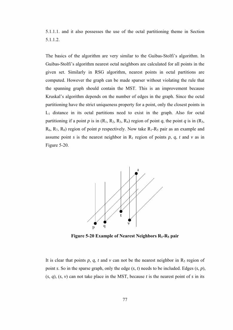
77

5.1.1.1. and it also possesses the use of the octal partitioning theme in Section

5.1.1.2.

The basics of the algorithm are very similar to the Guibas-Stolfi’s algorithm. In

Guibas-Stolfi’s algorithm nearest octal neighbors are calculated for all points in the

given set. Similarly in RSG algorithm, nearest points in octal partitions are

computed. However the graph can be made sparser without violating the rule that

the spanning graph should contain the MST. This is an improvement because

Kruskal’s algorithm depends on the number of edges in the graph. Since the octal

partitioning have the strict uniqueness property for a point, only the closest points in

L1 distance in its octal partitions need to exist in the graph. Also for octal

partitioning if a point p is in (R1, R2, R3, R4) region of point q, the point q is in (R5,

R6, R7, R8) region of point p respectively. Now take R1-R5 pair as an example and

assume point s is the nearest neighbor in R1 region of points p, q, t and v as in

Figure 5-20.

Figure 5-20 Example of Nearest Neighbors R1-R5 pair

It is clear that points p, q, t and v can not be the nearest neighbor in R5 region of

point s. So in the sparse graph, only the edge (s, t) needs to be included. Edges (s, p),

(s, q), (s, v) can not take place in the MST, because t is the nearest point of s in its

78

R5 region. It was proven before, that a point other than the nearest point in any octal

partition will be eliminated in the MST according to the cycle property. In the

Guibas-Stolfi’s algorithm all edges like the ones mentioned above will be in the

sparse graph which makes the sparse graph unnecessarily crowded. Therefore what

needs to be done is finding the nearest neighbors of all points in all octal regions

and taking the intersection of them. Intersection means including, if two points are

the nearest neighbors of each other in the opposing regions.

RST algorithm is mainly based on the above concepts. The algorithm is designed as

a sweep-line algorithm instead of a divide and conquer algorithm. It starts from a

point, does calculations for that point and continues to the next one in order without

any backtracking. It is explained in detail below.

The algorithm makes use of another property of octal partitioning. When a point

and its octal partitions are investigated, the equi-distant points from that point forms

a line segment in each region which can be seen in Figure 5-21. It can be also seen

from the figure that for regions R1, R2, R5 and R6 these line segments can be

represented by an equation in the form x+y=constant. For regions R3, R4, R7 and R8

the segments can be represented by an equation in the form x-y=constant.

Figure 5-21 Equi-Distant Points for Octal Partitioning

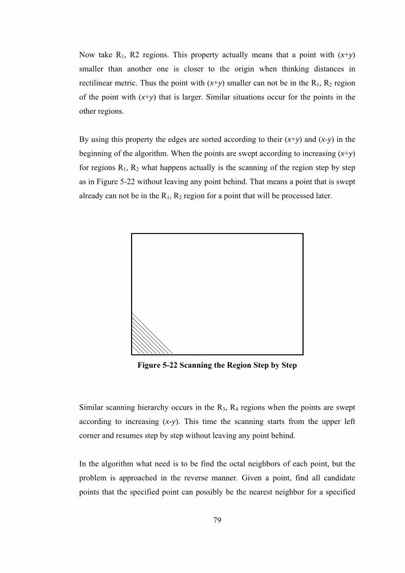
79

Now take R1, R2 regions. This property actually means that a point with (x+y)

smaller than another one is closer to the origin when thinking distances in

rectilinear metric. Thus the point with (x+y) smaller can not be in the R1, R2 region

of the point with (x+y) that is larger. Similar situations occur for the points in the

other regions.

By using this property the edges are sorted according to their (x+y) and (x-y) in the

beginning of the algorithm. When the points are swept according to increasing (x+y)

for regions R1, R2 what happens actually is the scanning of the region step by step

as in Figure 5-22 without leaving any point behind. That means a point that is swept

already can not be in the R1, R2 region for a point that will be processed later.

Figure 5-22 Scanning the Region Step by Step

Similar scanning hierarchy occurs in the R3, R4 regions when the points are swept

according to increasing (x-y). This time the scanning starts from the upper left

corner and resumes step by step without leaving any point behind.

In the algorithm what need is to be find the octal neighbors of each point, but the

problem is approached in the reverse manner. Given a point, find all candidate

points that the specified point can possibly be the nearest neighbor for a specified

80

octant. Now let’s consider R1 region in particular. As it was mentioned above, a

sweep line algorithm for this octant is constructed according to (x+y). During this

sweep an active set is constructed. The points in the active set are the ones whose

nearest neighbors are still not discovered yet. When a point is processed, all the

points in the active set are found which have that point in their R1 regions. In this

way, the whole point set is not searched for a point but only the points whose R1

regions are not discovered yet are taken in to account. Now suppose that a point s is

found in the active set when processing point p as p is in the R1 region of s. Since

the process is made in the form of non-decreasing (x+y) it is guaranteed that p is the

nearest neighbor of s in its R1 region. If there was another point that is closer to

point s it will be discovered before the point p is processed. Then the edge sp will

be included in the sparse graph and s will be removed from the active set. When the

processing of the point p is finished then it is added to the active set. Each point will

be added and deleted once from the active set.

The basic operation of the algorithm for a point p is to find in the sweeping

sequence a subset of active points such that p is in their R1 regions. Then the point p

will be referred as the nearest neighbor in R1 of the point q in this subset which is

closer to p in rectilinear metric. In this way we actually make the intersection of R1-

R5 regions which was discussed in the beginning of the section. Because when the

subset of active points is found that have p in their R1 region, actually p is found to

be the nearest R1 neighbor of those points. Then when the closest point in this

subset is connected to the graph, actually the R5 region of the point p is searched

and that closest point is the one that is the nearest R5 neighbor of point p. Also the

subset of these active points must be removed from the active set. Point p is the

nearest R1 neighbor of the points in this subset, but for the points other than the

closest one to point p, there is a closer point. So these points must be eliminated.

Since a point is deleted from the active set when a point that is in its R1 region is

found, no point in the active set can be in the R1 region of each other. Then the

following property holds for the points in the active set:

81

For any two points p and q that are in the active set it is guaranteed that p qx x≠ and

if p qx x< , then p p q qx y x y− ≤ − . This can be seen in the Figure 5-23:

Figure 5-23 Two Points that are not in the R1 Region of each other

Based on this property, the active set can be ordered in increasing order of x, which

also implies a non-decreasing order in x-y. The active set is ordered according to

this property and what needs to be done next is to find how it can be searched

efficiently. When a point p is swept, the points which have p in their R1 region

needs to be found, which means the points in the R5 region of p at the same time.

These points are characterized according to the following inequalities:

p

p p

x xx y x y≤− > −

(5.12)

Now to find the subset of active points which have p in their R1 regions, first the

largest element that have px x≤ in the active set is found. Then the other points in

the decreasing x order in the active set are proceeded until x-y becomes smaller than

p px y− .

When the sweeping process ends for the R1 region, also the R5 octant’s nearest

neighbors are found. Similar process occurs for also the other regions. For R2 region

82

the sweeping is kept in non-decreasing (x+y) also, and for R3 and R4 regions it is

kept in non-decreasing (x-y).

The changes will be made on the ordering of the active set. For R2 region any

element that is in the active set will not be in the R2 region of the other, so the

following properties occur according to Figure 5-24:

,q p q p

q p p p q q

x x y yif y y y x y x− ≠ − ≥ − < − (5.13)


According to the Equation(5.13) the active set for R2 region can be kept in non-

decreasing order of y. This also implies increasing order of y-x. Given a point p, the

points which have p in their R2 region must obey the following inequalities:

p

p p

y yy x y x

<− ≥ −

(5.14)

In order to find the subset of active points which have p in their R2 region, first

largest y such that py y< can be found and then by proceeding in decreasing order

of y in the active set until y-x becomes smaller than p py x− .

83

For R3 region any element that is in the active set will not be in the R3 region of the

other, so the following properties occur according to Figure 5-25:

,p q

q p q q p p

y yif y y x y x y

≠ < + ≤ + (5.15)


According to the Equation(5.15) the active set for R3 region can be kept in

decreasing order of y. This also implies non-increasing order of x+y. Given a point

p, the points which have p in their R3 region must obey the following inequalities:

p

p p

y yx y x y≥+ < +

(5.16)


smallest y such that py y≥ can be found and then by proceeding in increasing order

of y in the active set until x+y becomes larger than p px y+ .

For R4 region any element that is in the active set will not be in the R4 region of the

other, so the following properties occur according to Figure 5-26:

,

p p q q

p q p p q q

x y x yif x x x y x y

+ ≠ + ≤ + < +

(5.17)

84


According to the Equation(5.17) the active set for R4 region can be kept in non-

decreasing order of x. This also implies increasing order of x+y. Given a point p, the

points which have p in their R4 region must obey the following inequalities:

p

p p

x xx y x y

<+ ≥ +

(5.18)


largest x such that px x< can be found and then by proceeding in decreasing order

of x in the active set until x+y becomes smaller than p px y+ .

By the procedure mentioned above the spanning graph is generated. And now the

MST can be found using this sparse graph.

5.2.1.2. Calculating MST from RST

For calculating the MST from the spanning graph, the same procedure explained in

5.1.1.4. namely Kruskal’s MST algorithm is used, In Kruskal’s algorithm the edges

of the graph are sorted according to their gains. This sorting is used in the merging

binary tree step of the given pseudo code for the algorithm.

85

5.2.2. RST Edge Based Heuristics

The edge based heuristic used in RST takes its roots from the Edge-Based Heuristic

of Borah et al. [47]. The idea of the algorithm is starting with an initial minimum

spanning tree and then iteratively considering connecting a point to a nearby edge

and deleting the longest edge on the formed cycle. Next the idea of Borah and how

it is modified in the RST will be examined in more detail.

Borah’s algorithm uses an edge based update on the MST. Its main step can be

visualized easily with the help of Figure 5-27. It should be noted that the edges

shown in the figure are in Euclidean metric, but the actual distances are measured

by using the Rectilinear metric. This is preferred for clarity only.

Figure 5-27 Edge-Based Update

When point p is connected to point s1 in the upper figure, then a loop is formed in

the tree. As in GTCA algorithm this loop must be broken by removing the most

expensive edge in it. Now assume that for this example edge (b,c) is the most

expensive edge on the path from point b to point p. Thus this edge has to be

removed. Now by adding point s1 to the tree, then following modifications occur:

- Remove edge (a,b)

- Remove edge (b,c)

- Add edge (s1,a)

86

- Add edge (s1,b)

- Add edge (s1,p)

Hence it is observed that the procedure has added a new node to the tree and two

edges are replaced with three new edges in the tree. Following these modifications

the graph becomes a spanning tree for a new set of points including this extra node.

It can be observed that the total rectilinear costs of edge (s1,a) and edge (s1,b) is

equal to the cost of edge (a,b). Thus the total cost of these modifications is equal to:

1( ( , )) , ,gain adding point p to edge a b b c s p = − (5.19)

It can be seen in Equation (5.19) that when the rectilinear distance between point p

and point s1 is smaller than the rectilinear distance between point b and c, the gain

of adding point p to edge (a,b) reduces the cost of the total graph.

Borah’s algorithm starts with an initial minimum spanning tree and considers all

point-edge pairs in the graph whose size is equal to n2. In order to find the most

expensive edge in the cycle formed by each connected point-edge pair, a recursive

routine similar to depth first search is computed. This procedure starts with the

given edge as root and passes the maximum edge seen so far as a parameter to the

recursive calls. Each depth first search takes O(n) time and by applying this edge-

update procedure to all edges, this most expensive edge calculation procedure takes

O(n2) time. Then to keep the complexity at O(n2) only one point with largest gain is

held for each edge and O(n) point-edge pairs are sorted according to their gains.

Afterwards each point-edge pair is applied to the initial MST in a batched manner

starting from the one with the largest gain. Each point-edge pair is merged into the

tree if their gains did not change, which means that the edges that will be removed

for that particular point-edge pair is not deleted before.

Besides this implementation of the algorithm, Borah et al. have offered another

method in order to achieve the time complexity of O(nlgn). This was based on the

fact that, for a given edge, not all the points in the tree need to be considered as

point-edge pairs. The idea can be seen in Figure 5-27. For the edge (a,b), point e

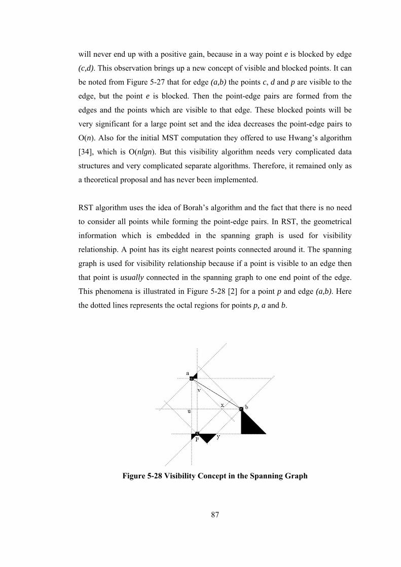
87

will never end up with a positive gain, because in a way point e is blocked by edge

(c,d). This observation brings up a new concept of visible and blocked points. It can

be noted from Figure 5-27 that for edge (a,b) the points c, d and p are visible to the

edge, but the point e is blocked. Then the point-edge pairs are formed from the

edges and the points which are visible to that edge. These blocked points will be

very significant for a large point set and the idea decreases the point-edge pairs to

O(n). Also for the initial MST computation they offered to use Hwang’s algorithm

[34], which is O(nlgn). But this visibility algorithm needs very complicated data

structures and very complicated separate algorithms. Therefore, it remained only as

a theoretical proposal and has never been implemented.

RST algorithm uses the idea of Borah’s algorithm and the fact that there is no need

to consider all points while forming the point-edge pairs. In RST, the geometrical

information which is embedded in the spanning graph is used for visibility

relationship. A point has its eight nearest points connected around it. The spanning

graph is used for visibility relationship because if a point is visible to an edge then

that point is usually connected in the spanning graph to one end point of the edge.

This phenomena is illustrated in Figure 5-28 [2] for a point p and edge (a,b). Here

the dotted lines represents the octal regions for points p, a and b.

Figure 5-28 Visibility Concept in the Spanning Graph

88

Since (a,b) is in the graph, point b is the nearest point in R3 region of point a and

also point a is the nearest point in R7 region of point b. So there can be no terminal

in region (a,x,b,z). Afterwards if point p is connected to point b in the spanning

graph, then point b is the nearest point in the R2 region of point p and also point p is

the nearest point in the R6 region of point b. Since (p,b) edge is in the spanning

graph there can be no terminal in region (p,y,b,x). If point p is connected to point a

in the spanning graph, then point a is the nearest point in the R8 region of point p

and also point p is the nearest point in the R1 region of point a. Since (p,a) edge is

in the spanning graph there can be no terminal in region (p,y,b,x). Thus according to

these properties point p is assumed to be visible to edge (a,b). On the other hand,

when there is no point between point p and edge (a,b), point p may not be

connected to edge (a,b) in the spanning graph when there is at least one point in

each of the shaded regions. This is because the points in the shaded regions are

nearer than the points mentioned. It is observed that such cases can cause loss of

information.

In the RST algorithm spanning graph is used for point-edge pair generation.

However it should be noted that there is no one-to-one correspondence between the

visibility and connection to the end points. For each edge in the Rectilinear

Minimum Spanning Tree (RMST), the end points of that edge are considered. Then

all neighbors of both endpoints in the Rectilinear Spanning Graph (RSG) are

considered as point components of point-edge pairs. Since the number of possible

point edge pairs is O(n) then the complexity of RSG is also O(n).

The same edge update procedure of Borah also applies to RST. After the initial

minimum spanning tree is formed by the Spanning Graph Algorithm, the point-edge

pairs are calculated. All point-edge pairs will be merged into MST and therefore

most expensive edges in the formed cycles should be found. Gains of these merging

processes are calculated and sorted afterwards. As a last step if the gain of the point-

edge pair in order has not been changed yet, three new edges will be connected to

the tree and two most expensive edges will be removed from the tree. The gain of a

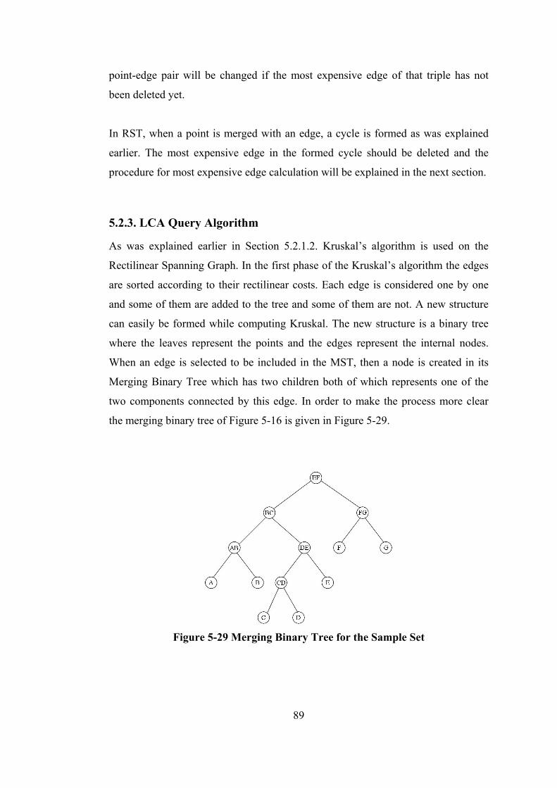
89

point-edge pair will be changed if the most expensive edge of that triple has not

been deleted yet.

In RST, when a point is merged with an edge, a cycle is formed as was explained

earlier. The most expensive edge in the formed cycle should be deleted and the

procedure for most expensive edge calculation will be explained in the next section.

5.2.3. LCA Query Algorithm

As was explained earlier in Section 5.2.1.2. Kruskal’s algorithm is used on the

Rectilinear Spanning Graph. In the first phase of the Kruskal’s algorithm the edges

are sorted according to their rectilinear costs. Each edge is considered one by one

and some of them are added to the tree and some of them are not. A new structure

can easily be formed while computing Kruskal. The new structure is a binary tree

where the leaves represent the points and the edges represent the internal nodes.

When an edge is selected to be included in the MST, then a node is created in its

Merging Binary Tree which has two children both of which represents one of the

two components connected by this edge. In order to make the process more clear

the merging binary tree of Figure 5-16 is given in Figure 5-29.

Figure 5-29 Merging Binary Tree for the Sample Set

90

It can be shown that the most expensive edge between two points is the least

common ancestor of these points in the corresponding merging binary tree. As an

example the most expensive edge between point A and point G is the edge (E,F) and

the most expensive edge between point A and point E is the edge (B,C). In RST in

order to find this longest edge between two points, Tarjan’s off-line least common

ancestor algorithm [62] is used.

In RST algorithm the maximum cost edge has to be found between a point and an

edge, which is a little different from Least Common Ancestor (LCA) procedure to

apply directly. What we need to do is to find the end point of the edge that was in

the same component in Kruskal computation before the edge is added to the MST.

It should be noted that this algorithm is embedded in the Kruskal computation.

Thus when an edge is to be added to the MST, it is added to the merging binary tree.

Then for each neighbor of the edge in the Rectilinear Spanning Graph, this edge’s

end point which is in the same component with the neighbor node and the neighbor

node itself will be added to LCA queries. Therefore Kruskal’s algorithm is modified

according to RST and the merging binary tree and the LCA queries are ready.

5.2.4. Tarjan’s Offline Least Common Ancestor Algorithm

Tarjan’s Offline Least Common Ancestor algorithm is used in RST to calculate the

least common ancestors for the computed LCA queries. The problem is called

offline because the entire request sequence can be seen before providing the first

answer. This algorithm is an important graph theory algorithm that has also

applications in many other fields such as computational biology [63] .

The algorithm works by performing a post-order tree traversal. When the algorithm

returns from processing a node, the pair list is examined to find out if there are any

ancestor calculations to be performed in the pair list or not. Namely, if u is the

current node under investigation and (u,v) is in the pair list, and also a recursive call

91

to v is already finished, then enough information is determined to calculate the least

common ancestors between u and v.

The progress of the algorithm can be seen in Figure 5-30. In the figure it is assumed

that a recursive call to D is about to finish. The nodes that have been visited are

shaded and the recursive calls for all nodes except the nodes on the path to node D

are already finished. When the recursive call to a node is finished that node is

marked. Also the closest node on the current access path to a visited node v is called

the anchor for node v. In Figure 5-30, A is the anchor of p, B is the anchor of q and

r is unanchored. In the algorithm all nodes that have the same anchor are assumed

to be on the same equivalence class and all nodes that are unvisited are assumed to

be on their own equivalence class. In the figure assume that (D,v) is in the pair list.

Then there are three possible cases:

- If v is unmarked, there is no information to compute the least common

ancestor of D and v.

- If v is marked but not in D’s sub-tree, then LCA of (D,v) is the anchor of v.

- If v is in D’s sub-tree, then LCA( D,v ) equals to D.

Figure 5-30 LCA Algorithm Progress

92

In order to determine the least common ancestors with the above algorithm, the

anchor must be identified at each time. After each recursive call returns the sub-tree

is combined into that point’s equivalence class and the anchor is updated. For

example after the recursive call to D returns as in Figure 5-30 all nodes that are in D

have changed their anchors to C from D.

5.3. Modified RST Algorithm

Investigating the BGA and RST algorithms in detail, one can conclude that some

parts of the two algorithms are very similar. For example both of them starts with an

initial sparse graph on which they try to find the rectilinear minimum spanning tree.

Then they add different structures to the minimum spanning tree and they both

compute the longest edge formed after this addition. A closer investigation on both

algorithms will be made and best parts of the algorithms in terms of performance

will be merged in the rest of this work.

First, the construction of the sparse graph will be investigated. The number of

selected edges is more in the BGA algorithm. When the initial graph gets a more

sparse nature, the Kruskal algorithm will deal with less number of edges, which

may cause it to run faster. In BGA, the edges are constructed through a recursive

algorithm, whereas the RST algorithm uses an iterative approach in a sweeping

manner. Recursive algorithms are not preferred when speed is desired because at

each recursion step the values are stored and then reloaded again. Also stack

overflows can occur at some point. This becomes a disadvantage when relatively

large instances are solved. Taking these facts into account, the RSG algorithm

should be taken as the initial spanning graph in the Modified RST algorithm.

The longest edge calculations are similar in both algorithms and they have been

implemented using different approaches. In BGA, first, parent and edge arrays are

constructed using Hierarchical Greedy Preprocessing (HGP) Algorithm. Then by

using these arrays longest edge can be determined between any given two terminals.

In RST merging binary tree are constructed initially and then Tarjan’s Offline Least

93

Common Ancestor algorithm is applied. When these are examined, RST algorithm

is conjectured to be more costly. Tarjan’s Offline Least Common ancestor

algorithm is also a recursive algorithm unlike the HGP algorithm. Therefore in the

Modified RST algorithm, we will adopt the BGA approach for longest edge

computations.

In BGA algorithm, triples are formed and then they are added to the tree. In RST

algorithm the neighbors of the edge in RSG are added to the tree. Since the

generation of triples requires a recursive approach again, it is not preferred in the

Modified RST algorithm. Since RSG is selected as an initial sparse graph, there is

no problem of selecting Borah’s algorithm for the Modified RST algorithm.

These assumptions and proposals made for the Modified RST algorithm need to be

verified. This is accomplished by profiling both of the algorithms where the results

are presented in Chapter 7.

94

CHAPTER 6

DISTRIBUTED VERSION OF MODIFIED RST

The Rectilinear Steiner Minimum Tree may be required to be computed for a large

number of times for a given physical design problem. In modern VLSI designs, also

there exist many large pre-routes. Therefore a very large amount of time may be

consumed for the Rectilinear Steiner Minimum Tree computation in a typical VLSI

design cycle. One way to reduce this time may be to find better heuristics that

calculates RSMT more efficiently. In another approach one may prefer to solve it

using many computers simultaneously rather than solving it in one computer only.

In this chapter, a distributed computing environment will be identified first that can

be used to compute the Rectilinear Steiner Minimum Tree in parallel. Then the

modified RST presented in detail in Chapter 5 will be parallelized such that it can

we can run it using many computers in parallel.

6.1. Computing Environment

Parallel programming consists of writing and running computer programs such that

a program runs simultaneously on several processors. These processors work all

together to achieve the computation task in a shorter time compared to one

processor case. The potential speedup in the execution time takes the attention of

many researchers for parallel computing [64].

There are mainly two types of parallel programming environments. One of them is

the shared memory environment and the other one is the distributed memory

95

environment. A shared memory environment is the one in which there are many

processors, each of which has access to the same common memory. This is an

advantage since all processors have access to all the data. However, the biggest

disadvantage is that it doesn't scale well to a large number of processors. Such

shared memory systems are also very expensive compared to a distributed memory

environment, which consists of many processors, each having its own local memory

space.

Network of Workstation (NOW) is a system, which is a kind of distributed memory

environment and is a good alternative to parallel computers since they can be set up

at relatively low cost [65]. This is because of having cheaper, faster and

commercially available of-the-shelf processors every day. In such an environment a

high degree of parallelism can be achieved by dividing the computation into

manageable subtasks and distributing these subtasks to the processor within the

cluster [66]. A network of workstation setup can contain desktops and workstations,

each of which is independent and autonomous systems themselves. The memory

can vary on each system, but the minimum memory on any of the components

should comply with the application. Theoretically, any number of nodes are

acceptable for setting up a NOW application, but the scalability may not be linear as

the number of nodes increases. The increase in performance should also be

comparable with the increase in cost. In a NOW setup, nodes are connected through

industry standard components and connections such as Ethernet [67]. An example

system can be seen in Figure 6-1.

96

Figure 6-1 A Sample NOW Structure

In a NOW structure, besides their autonomous tasks, every processor may cooperate

with each other for solving the same problem. Each processor may have its own

local copy of the problem instance in its local memory. When the program proceeds,

this data needs to be shared between the processors, which may be achieved by

some kind of a message passing system. PVM and MPI are the most popular

programs to implement message passing and synchronization among processes [68].

In this thesis work, MPI library will be used as a message passing library [69].

When an algorithm for distributed computing is designed, it is worth noting that

data exchange between the processors will have a relatively high cost. Although the

Ethernet is fast, a significant communication overhead may arise in the above

described system of workstations.

6.2. Distributed Algorithm Proposed for Modified RST

A distributed algorithm for the Modified RST will be proposed in this section by

parallelizing the major components of the Modified RST. Our proposal starts with

the parallelization of the Rectilinear Spanning Graph algorithm whose sequential

version is already explained in Section 5.2.1.1. and continues with the rest.

RSG algorithm is the backbone for the RST algorithm. Therefore, in order to

construct an efficient distributed algorithm, RSG has to be parallelized efficiently.

97

When the algorithm is investigated some parts of it seems naturally parallelizable.

For example octal regions can separately be solved because there is no relation

between the computations of the separate octal regions. Therefore each pair R1-R5,

R2-R6, R3-R7 and R4-R8 can be solved in different processors. However, this will

cause a problem if there are more than four processors. A more general procedure,

without any restriction on the number of processors will be more useful. The

following paragraphs describe a possible parallelization of RSG such that the

algorithm takes advantage of an increase in the number of processors.

In the first phase of the RSG algorithm for R1 and R2 regions the points have to be

sorted according to (x+y) and for R3 and R4 regions the points have to be sorted

according to (x-y). Then a master processor reads the data set and sends it to all

processors. It examines the data set, finds the maximum and minimum points both

in x and y-directions and also broadcasts these data to all processors, which will

identify the regions. Using this data, the whole region may be partitioned into equal

pieces depending on the number of processors. Each processor will process the

points that lie inside its defined region. Region partitioning idea is illustrated in

Figure 6-2.(a) for four processor case for R1 and R2 regions . A similar partitioning

approach is applicable for R3 and R4 regions as illustrated in Figure 6-2.(b) which is

drawn for number of processors is equal to 8. By assuming that the points are

scattered across the region uniformly, the regions can be selected such that their

area are equal.

98

Figure 6-2 Division of the Points to Predefined Regions

Each worker processor sorts its data according to non-decreasing gain. R1 region

will be investigated first; the others will be handled in the same manner. The

regions were divided to predefined halves depending on the number of processors

above. Now assume that there are eight processor assigned to these region pair.

Then the region is divided as can be seen in Figure 6-3. Starting from the regions

that have an arrow pointing upwards, the R1 nearest neighbors of the points will be

calculated. The process is the same as RSG algorithm, namely an active set will be

maintained whose elements consists of the points which have R1 region still not

have been discovered. Then for all points in that region it will be examined that if

that point is in the R5 region of the other. When all points in that region are

processed, R1 nearest neighbors of the points in that region are discovered except

for the points in the active set. According to the octal partitioning properties no

points are left behind other than the points in the active set whose R1 region is not

discovered because the points are sorted according to their (x+y).

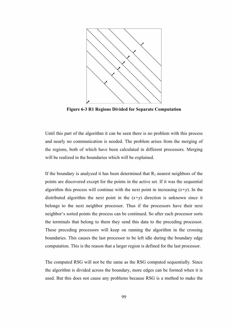
99

Figure 6-3 R1 Regions Divided for Separate Computation

Until this part of the algorithm it can be seen there is no problem with this process

and nearly no communication is needed. The problem arises from the merging of

the regions, both of which have been calculated in different processors. Merging

will be realized in the boundaries which will be explained.

If the boundary is analyzed it has been determined that R1 nearest neighbors of the

points are discovered except for the points in the active set. If it was the sequential

algorithm this process will continue with the next point in increasing (x+y). In the

distributed algorithm the next point in the (x+y) direction is unknown since it

belongs to the next neighbor processor. Thus if the processors have their next

neighbor’s sorted points the process can be continued. So after each processor sorts

the terminals that belong to them they send this data to the preceding processor.

These preceding processors will keep on running the algorithm in the crossing

boundaries. This causes the last processor to be left idle during the boundary edge

computation. This is the reason that a larger region is defined for the last processor.

The computed RSG will not be the same as the RSG computed sequentially. Since

the algorithm is divided across the boundary, more edges can be formed when it is

used. But this does not cause any problems because RSG is a method to make the

100

initial graph sparser. The extra edges will be eliminated in the Kruskal algorithm

without causing any harm.

By the above methodology, a spanning graph can be realized in a distributed

environment. Now the second step of the Modified RST algorithm is to run a

special type of Kruskal computation which will find the parent, edge arrays and the

LCA queries as well as the rectilinear minimum spanning tree. This step needs that

the edges are sorted according to their gains. So in the previous step when the RSG

algorithm is running, the processors will sort its points according to the rectilinear

distance and will send this list to all processors. Then each processor will run this

modified Kruskal algorithm after it has combined the list coming from the

processors. This Kruskal algorithm will run on the all processors separately in this

work because as disjoint set operations are used in the algorithm, the

communication overhead will become the bottleneck of the computation. Thus the

algorithm can be taught as a partially parallelized algorithm. It only recommends an

idea and will try to test if it is working.

Now every processor have parent, edge arrays, the rectilinear minimum spanning

tree and LCA queries which are the outputs of the previous algorithm. The LCA

queries will be divided across the processors according to the number of the

processors. Each LCA query is a point-edge pair indeed, so the processor will run

the Borah’s algorithm on them. The processor will merge the point to the edge and

will calculate the most expensive edge in the formed cycle. Since the processor has

the parent and edge arrays, it can calculate the most expensive edge easily and it can

calculate the gain of connecting that point-edge pair as explained in the sequential

algorithm. Then each processor sorts the point-edge pairs in terms of their gains and

sends this sorted list to the master processor. It has to be noted that the most

expensive edges that have been calculated are also been sent to the master processor.

The master processor combines the gains according to the sorted order and then

applies these point-edge pairs to the minimum spanning tree as in sequential

algorithm.Equation Chapter (Next) Section 1

101

CHAPTER 7

COMPUTATIONAL WORK

Both algorithms defined in the previous chapters are implemented using Microsoft

Visual C++ 6.0 on a Microsoft Windows machine. The stack size is not changed

and remained as 1MB as default. BGA algorithm that can be run readily in a Linux

machine was given in [53]. First this code is modified to run on Windows machines.

Then the RST algorithm is implemented following the pseudocode presented in

Chapter 5. We ran both programs and analyzed them in detail using a profiler. The

time consuming parts of the algorithms are identified and the assumptions made on

the algorithms are verified. Modified RST algorithm is then implemented as defined

in Chapter 5. Both programs have been run and results have been taken on a 3,2

GHz Pentium IV processor that has 2GB memory.

The parallel code proposed for the modified algorithm in the previous chapter is

implemented using the message passing interface (MPI). MPICH, an MPI

implementation of Argonne National Laboratory, is used as the MPI library. The

code is tested on a Windows cluster of eight machines all having a 2,4 GHz

Pentium IV processor and 512 MB of memory. Test results have been obtained and

will be presented below.

7.1. Implementation of RST

RST algorithm is implemented according to the pseudocode given in the previous

chapter. However there is an addition to that code. After a single pass of the RST

algorithm, there may still be a possibility of improvement. In the paper by Zhou [2]

102

this fact is taken into account and he has suggested to compute the sparse graph

once and then run the rest of the program five times. However it is not clearly stated

how the Steiner points that are found after the first pass will be handled in the

following additional passes. For this part of the algorithm the following procedure

is followed:

The first pass of the algorithm is carried out exactly according to the pseudocode.

Then bypassing the sparse graph generation, the algorithm is applied five times if

there are any improvements in the previous pass. In each pass Modified Kruskal

Algorithm is slightly modified and adding the edge to the MST phase is skipped

since the MST is generated already. Also it was noted that in the least common

ancestor queries construction phase, the algorithm seeks for the RSG neighbors of

the points that construct the edges. But after the first pass of the algorithm some

edges have a Steiner point. Since the Steiner points do not have neighbors in the

RSG, only the neighbors of the terminals in the edges will be considered for LCA

queries.

Another modification is at the end of each pass of the algorithm, the Steiner points

which have degree of two will be deleted and edges will be adjusted accordingly.

This procedure was given in Section 4.4.3. The Steiner points with degree two or

less are deleted because if they are not deleted, the algorithm will treat them like

normal terminals but they will not necessarily be included in the graph. Of course

after deleting these nodes the graph must not remain unconnected. For this reason if

the deleted Steiner point has degree two, both of the edges connecting to that point

will be deleted and the other points forming the deleted edges will be connected to

each other. Here attention has to be taken for special cases. For example in some

cases two Steiner points which have degree two can be connected to each other.

Also for Steiner points with degree one, that edge containing it can be taken out of

the graph.

After mentioning the differences when implementing the algorithm, now the basic

data structures used throughout the algorithm will be explained. Using the right data

103

structures is very important for this work because the performance of the algorithms

is measured in terms of size of the problem and the time to solve it. With a well-

designed data structure, a variety of critical operations can be performed using

fewer resources.

7.1.1. Balanced Binary Search Tree

The backbone of the algorithm is rectilinear spanning graph (RSG) construction

part and the key concept there is to keep an efficient active set. The active set is

defined as an ordered structure and insertion, deletion and search operations are

performed on it. So it will be a good choice to select binary search trees to

implement it. In a binary search tree all nodes to the left of the current node have

key value smaller than that of the current node and all nodes to the right of the

current node have key value larger than that of the current node. Most of the

operations’ complexity in a binary search tree depends on the height of the tree. For

a binary tree of n nodes these operations run in O(nlgn) average time but O(n) worst

case time.

A self-balancing binary search tree or height-balanced binary search tree seams

suitable for this thesis work. Balanced binary search tree is a binary search tree that

attempts to keep its height, or the number of levels of the nodes beneath the root, as

small as possible at all times, automatically. Namely with some effort to balance the

tree, all operations are guaranteed to run in O(lgn) time in the worst case. The

difference between the binary search tree (Figure 7-1.(a) ) and balanced binary

search tree (Figure 7-1.(b) ) can be depicted in Figure 7-1.

104

Figure 7-1 Binary Search Tree and Balanced Binary Search Tree

Some previously developed balanced binary search trees in the literature are AVL

Trees, Red-Black Trees and AA-Trees [63]. AA-Trees [70] have been selected for

their ease of implementation while providing a similar performance compared to

others. AA-Trees store a value called level where level represents the number of left

links of a node. In an AA-Tree the left child of a node must be one level lower than

its parent, and the right child of a node may be at most one level lower than the

parent. A binary search tree is shown in Figure 7-2.(a). In Figure 7-2.(b) besides the

key values, the level values are also presented in each node and this tree is

equivalent to the tree in Figure 7-2.(c).

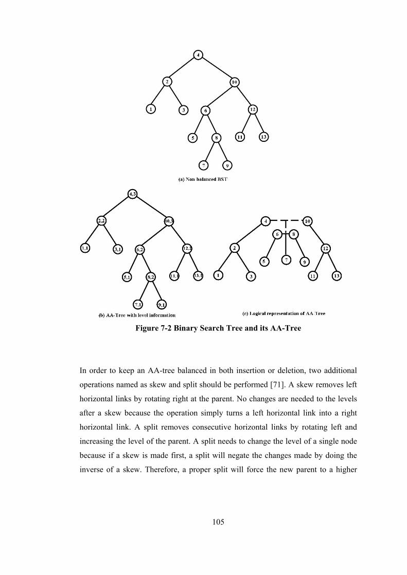
105

Figure 7-2 Binary Search Tree and its AA-Tree

In order to keep an AA-tree balanced in both insertion or deletion, two additional

operations named as skew and split should be performed [71]. A skew removes left

horizontal links by rotating right at the parent. No changes are needed to the levels

after a skew because the operation simply turns a left horizontal link into a right

horizontal link. A split removes consecutive horizontal links by rotating left and

increasing the level of the parent. A split needs to change the level of a single node

because if a skew is made first, a split will negate the changes made by doing the

inverse of a skew. Therefore, a proper split will force the new parent to a higher

106

level. A skew operation can be seen in Figure 7-3.(a) and a split operation can be

seen in Figure 7-3.(b).

Figure 7-3 Skew and Split Operations

This basic definition of AA-Tree is not sufficient to be used in our algorithm and

need some more additions. Besides addition and deletion operations, successor and

predecessor information are also needed. Therefore parent information will be kept

and updated in all operations. In standard AA-trees, when multiple values need to

be inserted, they are normally discarded. To overcome this issue for RST a pointer

that can hold duplicated values is inserted in each node and they are maintained at

all operations.

Another data structure that has importance in RST algorithm is disjoint set classes.

They are both used in Modified Kruskal’s algorithm and Tarjan’s offline least

common ancestor algorithm.

7.1.2. Disjoint-Set Class

Some applications involve grouping elements into a collection of disjoint sets [57].

Two basic operations are finding which set a given element belongs to and uniting

two sets. So the algorithm solving disjoint-set data structure is generally referred as

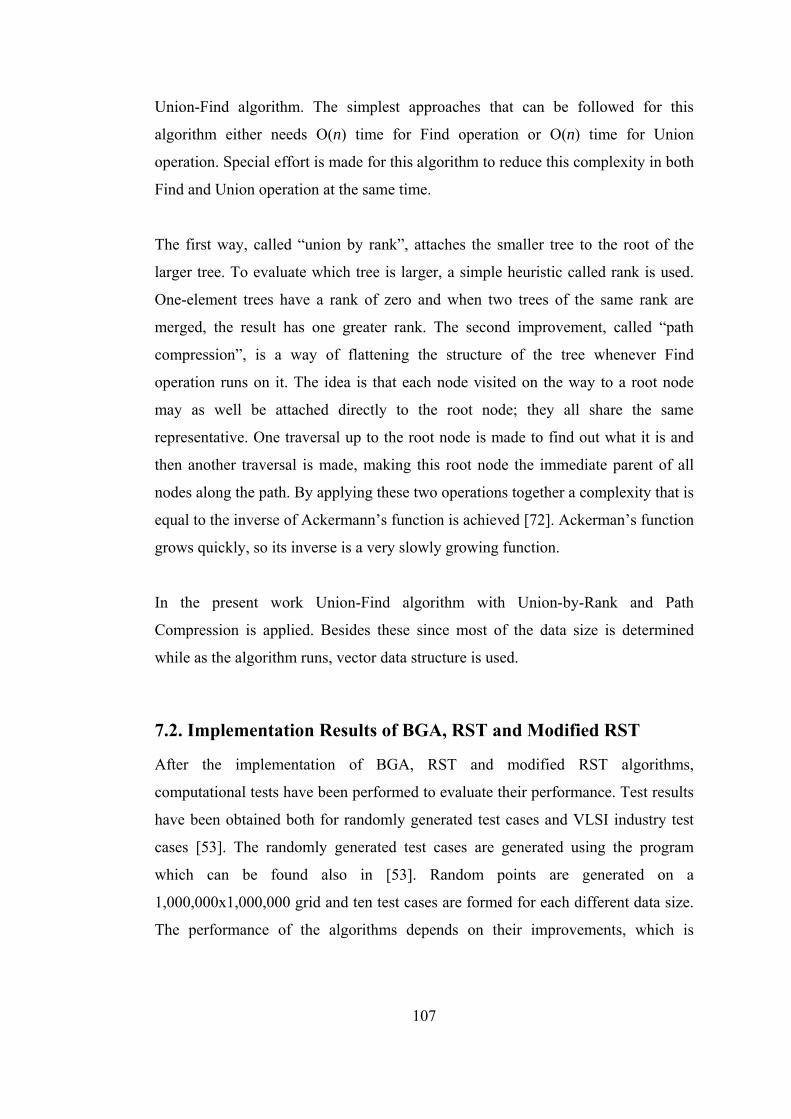
107

Union-Find algorithm. The simplest approaches that can be followed for this

algorithm either needs O(n) time for Find operation or O(n) time for Union

operation. Special effort is made for this algorithm to reduce this complexity in both

Find and Union operation at the same time.

The first way, called “union by rank”, attaches the smaller tree to the root of the

larger tree. To evaluate which tree is larger, a simple heuristic called rank is used.

One-element trees have a rank of zero and when two trees of the same rank are

merged, the result has one greater rank. The second improvement, called “path

compression”, is a way of flattening the structure of the tree whenever Find

operation runs on it. The idea is that each node visited on the way to a root node

may as well be attached directly to the root node; they all share the same

representative. One traversal up to the root node is made to find out what it is and

then another traversal is made, making this root node the immediate parent of all

nodes along the path. By applying these two operations together a complexity that is

equal to the inverse of Ackermann’s function is achieved [72]. Ackerman’s function

grows quickly, so its inverse is a very slowly growing function.

In the present work Union-Find algorithm with Union-by-Rank and Path

Compression is applied. Besides these since most of the data size is determined

while as the algorithm runs, vector data structure is used.

7.2. Implementation Results of BGA, RST and Modified RST

After the implementation of BGA, RST and modified RST algorithms,

computational tests have been performed to evaluate their performance. Test results

have been obtained both for randomly generated test cases and VLSI industry test

cases [53]. The randomly generated test cases are generated using the program

which can be found also in [53]. Random points are generated on a

1,000,000x1,000,000 grid and ten test cases are formed for each different data size.

The performance of the algorithms depends on their improvements, which is

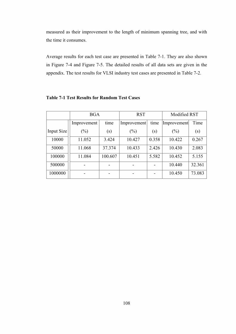
108

measured as their improvement to the length of minimum spanning tree, and with

the time it consumes.

Average results for each test case are presented in Table 7-1. They are also shown

in Figure 7-4 and Figure 7-5. The detailed results of all data sets are given in the

appendix. The test results for VLSI industry test cases are presented in Table 7-2.

Table 7-1 Test Results for Random Test Cases

BGA RST Modified RST

Input Size

Improvement

(%)

time

(s)

Improvement

(%)

time

(s)

Improvement

(%)

Time

(s)

10000 11.052 3.424 10.427 0.358 10.422 0.267

50000 11.068 37.374 10.433 2.426 10.430 2.083

100000 11.084 100.607 10.451 5.582 10.452 5.155

500000 - - - - 10.440 32.361

1000000

- - - - 10.450 73.083

109

Figure 7-4 Improvement of MST for Random Instances

Figure 7-5 Run-time of Algorithms for Random Instances

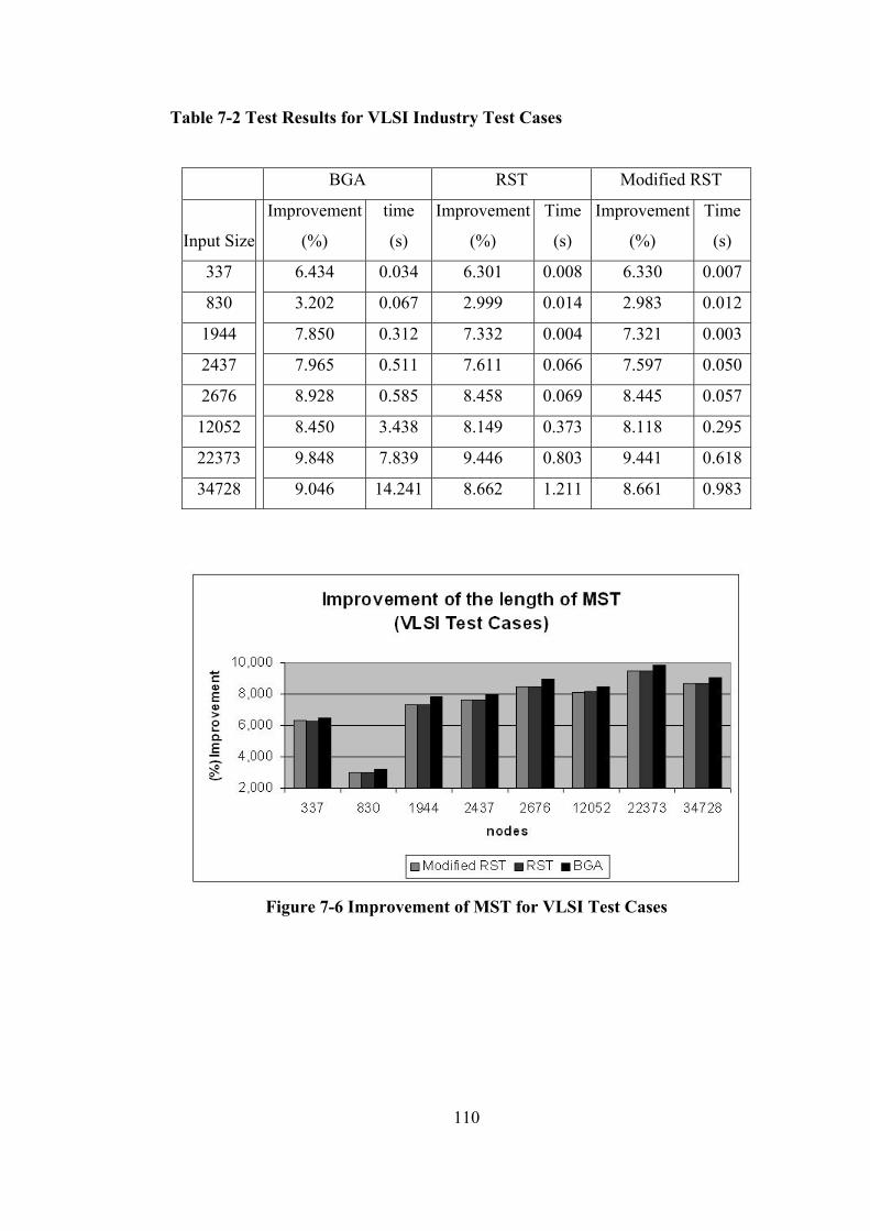
110

Table 7-2 Test Results for VLSI Industry Test Cases


Input Size

Improvement

(%)

time

(s)

Improvement

(%)

Time

(s)

Improvement

(%)

Time

(s)

337 6.434 0.034 6.301 0.008 6.330 0.007

830 3.202 0.067 2.999 0.014 2.983 0.012

1944 7.850 0.312 7.332 0.004 7.321 0.003

2437 7.965 0.511 7.611 0.066 7.597 0.050

2676 8.928 0.585 8.458 0.069 8.445 0.057

12052 8.450 3.438 8.149 0.373 8.118 0.295

22373 9.848 7.839 9.446 0.803 9.441 0.618

34728 9.046 14.241 8.662 1.211 8.661 0.983

Figure 7-6 Improvement of MST for VLSI Test Cases

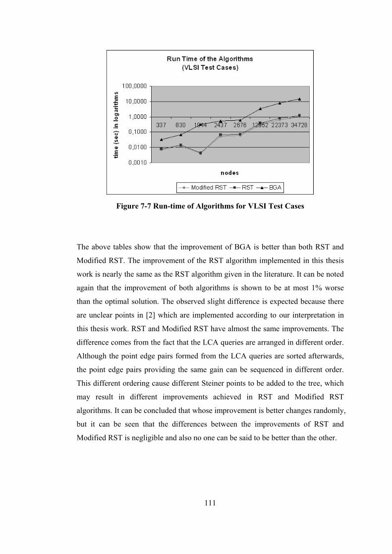
111

Figure 7-7 Run-time of Algorithms for VLSI Test Cases

The above tables show that the improvement of BGA is better than both RST and

Modified RST. The improvement of the RST algorithm implemented in this thesis

work is nearly the same as the RST algorithm given in the literature. It can be noted

again that the improvement of both algorithms is shown to be at most 1% worse

than the optimal solution. The observed slight difference is expected because there

are unclear points in [2] which are implemented according to our interpretation in

this thesis work. RST and Modified RST have almost the same improvements. The

difference comes from the fact that the LCA queries are arranged in different order.

Although the point edge pairs formed from the LCA queries are sorted afterwards,

the point edge pairs providing the same gain can be sequenced in different order.

This different ordering cause different Steiner points to be added to the tree, which

may result in different improvements achieved in RST and Modified RST

algorithms. It can be concluded that whose improvement is better changes randomly,

but it can be seen that the differences between the improvements of RST and

Modified RST is negligible and also no one can be said to be better than the other.

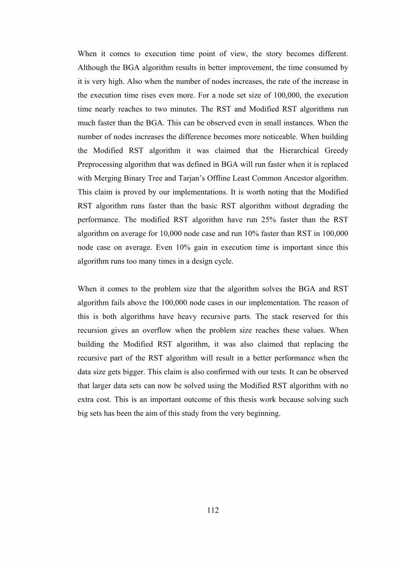
112

When it comes to execution time point of view, the story becomes different.

Although the BGA algorithm results in better improvement, the time consumed by

it is very high. Also when the number of nodes increases, the rate of the increase in

the execution time rises even more. For a node set size of 100,000, the execution

time nearly reaches to two minutes. The RST and Modified RST algorithms run

much faster than the BGA. This can be observed even in small instances. When the

number of nodes increases the difference becomes more noticeable. When building

the Modified RST algorithm it was claimed that the Hierarchical Greedy

Preprocessing algorithm that was defined in BGA will run faster when it is replaced

with Merging Binary Tree and Tarjan’s Offline Least Common Ancestor algorithm.

This claim is proved by our implementations. It is worth noting that the Modified

RST algorithm runs faster than the basic RST algorithm without degrading the

performance. The modified RST algorithm have run 25% faster than the RST

algorithm on average for 10,000 node case and run 10% faster than RST in 100,000

node case on average. Even 10% gain in execution time is important since this

algorithm runs too many times in a design cycle.

When it comes to the problem size that the algorithm solves the BGA and RST

algorithm fails above the 100,000 node cases in our implementation. The reason of

this is both algorithms have heavy recursive parts. The stack reserved for this

recursion gives an overflow when the problem size reaches these values. When

building the Modified RST algorithm, it was also claimed that replacing the

recursive part of the RST algorithm will result in a better performance when the

data size gets bigger. This claim is also confirmed with our tests. It can be observed

that larger data sets can now be solved using the Modified RST algorithm with no

extra cost. This is an important outcome of this thesis work because solving such

big sets has been the aim of this study from the very beginning.

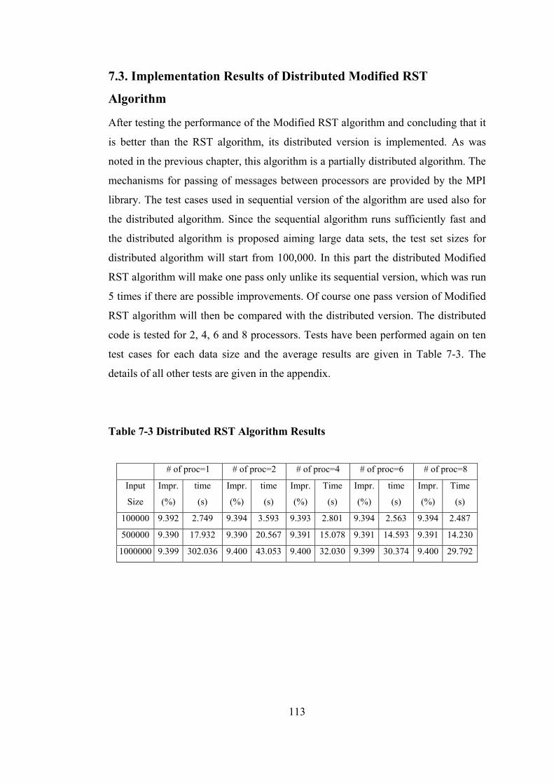
113

7.3. Implementation Results of Distributed Modified RST

Algorithm

After testing the performance of the Modified RST algorithm and concluding that it

is better than the RST algorithm, its distributed version is implemented. As was

noted in the previous chapter, this algorithm is a partially distributed algorithm. The

mechanisms for passing of messages between processors are provided by the MPI

library. The test cases used in sequential version of the algorithm are used also for

the distributed algorithm. Since the sequential algorithm runs sufficiently fast and

the distributed algorithm is proposed aiming large data sets, the test set sizes for

distributed algorithm will start from 100,000. In this part the distributed Modified

RST algorithm will make one pass only unlike its sequential version, which was run

5 times if there are possible improvements. Of course one pass version of Modified

RST algorithm will then be compared with the distributed version. The distributed

code is tested for 2, 4, 6 and 8 processors. Tests have been performed again on ten

test cases for each data size and the average results are given in Table 7-3. The

details of all other tests are given in the appendix.

Table 7-3 Distributed RST Algorithm Results

# of proc=1 # of proc=2 # of proc=4 # of proc=6 # of proc=8

Input

Size

Impr.

(%)

time

(s)

Impr.

(%)

time

(s)

Impr.

(%)

Time

(s)

Impr.

(%)

time

(s)

Impr.

(%)

Time

(s)

100000 9.392 2.749 9.394 3.593 9.393 2.801 9.394 2.563 9.394 2.487

500000 9.390 17.932 9.390 20.567 9.391 15.078 9.391 14.593 9.391 14.230

1000000 9.399 302.036 9.400 43.053 9.400 32.030 9.399 30.374 9.400 29.792

114

Figure 7-8 Run-time of the Distributed Algorithm

It can be observed from the above table that the improvement is pretty much the

same for all tests. The difference again may come from the possible different

orderings of the LCA queries and possibly from RSG part in the distributed version

which can have some extra edges.

The execution time needs to be examined in detail. For relatively small instances,

the algorithm for one processor runs faster than the two processor case. This is

because of the fact that the communication time is higher than the computation time.

As the number of processors increases the computation cost decreases but the

communication cost does not. As a result the overall time cost of the algorithm

decreases, but not in an efficient manner. In order to investigate this fact, a

1,000,000 terminal test case is taken and analyzed in detail. RSG is a backbone of

this algorithm, so its performance is examined and given in Table 7-4. First, the

result of RSG for the sequential algorithm and then the result of its distributed

version are given. The first recorded time is the maximum of each processors

completion time of RSG calculations in their partitions, and the second recorded

time is the time when each processor gets the overall sparse graph.

115

Table 7-4 Performance of RSG algorithm in distributed algorithm


RSG Time (sec) 13.105 8.466 5.693 4.222 3.506

After Broadcast (sec) - 22.220 13.556 12.671 12.471

As the number of processors increases, the RSG computation cost decreases almost

linearly. But after the broadcast the overall cost is nearly the same. It can be

concluded that as the number of processors increases the communication cost

increases also. This is because such a broadcast is implemented as unicast

operations in MPI. By using more appropriate methods or by using faster

communication links, this performance can be improved. However since the RSG

becomes faster it can still be concluded that the proposed algorithm is promising.

Another observation made from the above test results is that for the 1,000,000

terminal case the performance of one processor becomes bad. This is because for

that size the 512 MB RAM becomes the bottleneck and swapping operations on

memory to the hard disk start at this size. On the other hand for more than one

processor this size of data does not cause any problem. This performance of clusters

is the result of the increase in resources.

It can finally be concluded that although the distributed algorithm can not provide

linear speedup, it is still useful when the data size is relatively big.


116

CHAPTER 8

CONCLUSION

The Steiner Tree Problem is one of the fundamental problems in “Graph Theory”. It

is widely used in Physical Design phase of VLSI in which only horizontal and

vertical lines can be used due to technological constraints. The Steiner Tree version

used for VLSI Physical Design is the Rectilinear Steiner Tree which only consists

of rectilinear lines.

The Rectilinear Steiner Minimum Tree (RSMT) is defined as a tree that

interconnects a set of terminals by only using horizontal and vertical line segments

aiming to achieve minimum total length. It is different than the famous spanning

tree problem because extra nodes, called Steiner points, can be used in the solution.

The problem is shown to be NP-complete which reduces the hope of finding

efficient exact algorithms. In recent years successful exact algorithms have been

designed for sizes up to a thousand nodes. However, in this thesis work the aim is

solving the problem for sizes such as millions of nodes which eliminates the

possibility of using exact algorithms. This is the reason of using heuristics in this

study. The Rectilinear Steiner Minimum Tree Problem is solved many times

throughout a design so such a scalable algorithm is needed also for big data sets.

In order to solve the problem an extensive literature survey has been made

especially for approximation algorithms. Exact algorithms have also been studied to

investigate the proposed methods. It has been observed that most of the heuristics

start with minimum spanning tree and are updated with different algorithms. The

algorithms have been compared in terms of their performance keeping the focus on

117

the solution of relatively big sized problems. The performance has been measured

in terms of the length of the formed tree, the time that the algorithm takes to run and

the size of the problem it can solve. Another issue that has been taken into account

during the comparison between the algorithms is their adaptability for parallel

implementations.

Two recently developed algorithms have been selected according to their

performance namely Kahng’s BGA algorithm and Zhou’s RST algorithm. Both of

which have been shown to be suitable for problem sizes such as 100,000 nodes.

Both algorithms start with constructing a sparse graph on which initial minimum

spanning tree will be calculated and reduce the size of the minimum spanning tree.

To achieve this, the BGA algorithm uses Zelikovsky’s GTCA algorithm whereas

the RST algorithm uses Borah’s algorithm. Similar blocks of the algorithms have

been compared with each other first and their performances have been analyzed by

using a profiler. In this way the faster parts of the two algorithms have been

identified. The recursive parts have been removed because when a recursive routine

is implemented on a computer the registers are stored in a stack which makes the

algorithm slower. Besides as the input size becomes larger the stack can be

overflowed. As a result a modified algorithm has been proposed and implemented

in the thesis work.

In order to solve larger problems, a distributed version of the modified algorithm

has been studied. Some parts of the algorithm appeared costly to be implemented on

a distributed environment. So a partially distributed algorithm has been proposed

and its performance has been investigated accordingly.

The BGA algorithm for Linux that has been obtained at the end of the literature

survey has been modified to run on Windows. The RST algorithm has been

implemented in C++ language. Using the profiler results it has been concluded that

the modified algorithm can run faster than both of the algorithms. This fact has been

verified by tests conducted using random input sets and also with VLSI test cases.

The performance has been calculated in terms of time, improvement of MST and

118

the size of the node set that the algorithm solves. The BGA algorithm has been

found to be the best performing algorithm in terms of improvement, where the

improvements of RST and Modified RST can be rated as nearly equal. Their

performances have been found 1% worse than the BGA algorithm on average.

When the algorithms have been compared in terms of their timing performance,

BGA algorithm becomes the worst. The difference between timing performance

increases when the input set becomes larger. When the RST and Modified RST

algorithms have been compared it is concluded that the Modified RST algorithm is

faster in all data sizes. This speed up changes but it ranges from 10% to 25%. On

the solvable data set size the BGA and RST seem to be worse than the Modified

RST.

The first contribution of this work is proposing a modified algorithm that is formed

by analyzing and profiling the BGA and RST algorithms and then determining

faster blocks and removing recursive parts. Tests have been carried out on this

algorithm and shown that it can solve bigger data sets while providing a speed up

without degrading the performance.

The second contribution of this work is proposing a partially modified algorithm.

The distributed algorithm has been implemented by using MPI. The algorithm is

designed for large data sets so no tests have been made for small data sets. Tests

have been conducted on an eight computer cluster with different number of

processors. Results show that with increasing number of computers, the run time of

the algorithm decreases. But the rate of the decrease has not been as expected. The

main reason of it has been the communication overhead. It has been shown that the

RSG can be computed efficiently on a distributed environment but when the edges

have been gathered and broadcast through the communication medium the

performance of RSG becomes nearly the same as sequential RSG algorithm. Since

MPI converts broadcast operations to unicast operations, the communication

increases compared with processor computation load. Thus by using a faster link

and more importantly by using a more suitable message passing library than MPI

the performance can be improved.

119

On the other hand as the input size becomes relatively large the memory overflow

becomes a problem. At some point, memory gets full and swapping operations with

the hard disk begins slowing down the computation. Here using a cluster have

provided a gain in time by increasing the resources.

The partially modified algorithm can be improved as a future work. The idea

proposed for the distributed algorithm is useful but some further modifications can

be made on it. This partially parallelized algorithm can be modified to perform

better by using a more suitable message passing library than MPI which handles

collective communications better. Another improvement can be using a faster

communication medium. With these two the communication overhead can be

decreased. Also the sequential part of the algorithm that is not parallelized in this

work can be made to run in parallel. This can be provided by implementing a

successful Union-Find algorithm for the disjoint set data structure for distributed

environment.


120

REFERENCES

1. Kahng, A.B., I.I. Mandoiu, and A.Z. Zelikovsky. Highly scalable algorithms

for rectilinear and octilinear steiner trees. in In Proc. Asia South Pacific Design Automation Conf. 2003: p. 827-833.

2. Zhou, H., Efficient Steiner Tree Construction Based on Spanning Graphs. Computer-Aided Design of Integrated Circuits and Systems, IEEE Transactions on, 2004. 23(5): p. 704-710.

3. Hwang, F.K., D.S. Richards, and P. Winter, The Steiner tree problem. 1992: North-Holland.

4. Jarník, V. and M. Kössler, O minimálních grafech, obsahujících n danıch bodu. Casopis pro pestování matematiky a fysiky, 1934: p. 223-235.

5. Courant, R. and H. Robbins, What is Mathematics? 1941, Oxford University Press, New York.

6. Melzak, Z.A., On the problem of Steiner. Canad. Math. Bull, 1961. 4(2): p. 143-150.

7. Gilbert, E.N. and H.O. Pollak, Steiner Minimal Trees. SIAM Journal on Applied Mathematics, 1968. 16(1): p. 1-29.

8. Hanan, M., On Steiner's Problem with Rectilinear Distance. SIAM Journal on Applied Mathematics, 1966. 14(2): p. 255-265.

9. Hakimi, S.L., Steiner’s problem in graphs and its implications. Networks, 1971. 1(2): p. 113–133.

10. Ivanov, A.O. and A.A. Tuzilin, Minimal networks: the Steiner problem and its generalizations. 1994: CRC Press.

11. Karpinski, M., Mandoiu, II, A. Olshevsky, and A. Zelikovsky, Improved Approximation Algorithms for the Quality of Service Multicast Tree Problem. Algorithmica, 2005. 42(2): p. 109-120.

12. Penny, D., M.D. Hendy, and M.A. Steel, Progress with methods for constructing evolutionary trees. Trends in Ecology & Evolution, 1992. 7(3): p. 73–79.

13. Gerez, S.H., Algorithms for VLSI Design Automation. 1999: John Wiley & Sons, Inc. New York, NY, USA.

14. Cohoon, J., J. Karro, and J. Lienig, Evolutionary algorithms for the physical design of VLSI circuits. Natural Computing Series, 2003: p. 683-711.

15. Areibi, S., M. Xie, and A. Vannelli, An efficient rectilinear Steiner tree algorithm for VLSI global routing. Electrical and Computer Engineering, 2001. Canadian Conference on, 2001. 2: p. 1067-1072.

16. Sherwani, N.A., Algorithms for VLSI Physical Design Automation. 1995: Kluwer Academic Publishers Norwell, MA, USA.

17. Kahng, A.B. and G. Robins, On Optimal Interconnections for Vlsi. 1994: Kluwer Academic Publishers.

121

18. Zachariasen, M., The Rectilinear Steiner Tree Problem: A Tutorial. Steiner Trees in Industry, 2001. 11: p. 467–507.

19. Garey, M.R. and D.S. Johnson, The Rectilinear Steiner Tree Problem is NP-Complete. SIAM Journal on Applied Mathematics, 1977. 32(4): p. 826-834.

20. Garey, M.R., D.S. Johnson, and L.J. Stockmeyer, Some Simplified NP-Complete Graph Problems. TCS, 1976. 1(3): p. 237-267.

21. Hwang, F.K., On Steiner Minimal Trees with Rectilinear Distance. SIAM Journal on Applied Mathematics, 1976. 30(1): p. 104-114.

22. Yang, Y. and O. Wing, Suboptimal algorithm for a wire routing problem. Circuits and Systems, IEEE Transactions on [legacy, pre-1988], 1972. 19(5): p. 508-510.

23. Hetzel, A., Verdrahtung im VLSI-Design: Spezielle Teilprobleme und ein sequentielles Losungsverfahren, Ph. D. thesis, University of Bonn, 1995.

24. Salowe, J.S. and D.M. Warme, Thirty-Five Point Rectilinear Steiner Minimal Trees in a Day. Networks, 1995. 25(2): p. 69-87.

25. Fößmeier, U. and M. Kaufmann, Solving Rectilinear Steiner Tree Problems Exactly in Theory and Practice. Proceedings of the 5th Annual European Symposium on Algorithms, 1997: p. 171-185.

26. Winter, P., An algorithm for the Steiner problem in the euclidean plane. Networks(New York, NY), 1985. 15(3): p. 323-345.

27. Warme, D.M., Spanning Trees in Hypergraphs with Applications to Steiner Trees. 1998, University of Virginia.

28. Warme, D.M., P. Winter, and M. Zachariasen, Exact Algorithms for Plane Steiner Tree Problems: A Computational Study, Advances in Steiner trees. Advances in Steiner Trees. Norwell, Massachusetts: Kluwer Academic Publishers, pp, 2000: p. 81-116.

29. Zachariasen, M., Rectilinear full Steiner tree generation. Networks, 1999. 33(2): p. 125-143.

30. Warme, D.M., P. Winter, and M. Zachariasen, GeoSteiner 3.1 Department of Computer Science, University of Copenhagen (DIKU) http://www.diku.dk/geosteiner Last Updated: 07.01.2006

31. Emanet, N. and C. Özturan, Solving the Rectilinear Steiner Minimal Tree Problem with a Branch and Cut Algorithm. International Scientific Journal of Computing, 2004. 3(2).

32. Koch, T. and A. Martin, Solving Steiner tree problems in graphs to optimality. Networks, 1998. 32(3): p. 207-232.

33. Winter, P., Reductions for the rectilinear Steiner tree problem. Networks(New York, NY), 1995. 26(4): p. 187-198.

34. Hwang, F.K., An O (n log n) Algorithm for Rectilinear Minimal Spanning Trees. Journal of the ACM (JACM), 1979. 26(2): p. 177-182.

35. Yao, A.C.C., On Constructing Minimum Spanning Trees in k-Dimensional Spaces and Related Problems. SIAM J. Comput., 1982. 11(4): p. 721-736.

36. Ho, J.M., G. Vijayan, and C.K. Wong, New algorithms for the rectilinear Steiner tree problem. Computer-Aided Design of Integrated Circuits and Systems, IEEE Transactions on, 1990. 9(2): p. 185-193.

37. Zelikovsky, A.Z., An 11/6-approximation algorithm for the network steiner problem. Algorithmica, 1993. 9(5): p. 463-470.

http://www.diku.dk/geosteiner

122

38. Zelikovsky, A.Z., An 11/8-approximation Algorithm for the Steiner Problem on Networks with Rectilinear Distance. Coll. Math. Soc. J. Bolyai, 1992. 60: p. 733-745.

39. Berman, P. and V. Ramaiyer, Improved approximations for the Steiner tree problem. Proceedings of the third annual ACM-SIAM symposium on Discrete algorithms, 1992: p. 325-334.

40. Foßmeier, U., Faster Approximation Algorithms for the Rectilinear Steiner Tree Problem. Discrete and Computational Geometry, 1997. 18(1): p. 93-109.

41. Arora, S., Polynomial time approximation schemes for Euclidean traveling salesman and other geometric problems. Journal of the ACM (JACM), 1998. 45(5): p. 753-782.

42. Kahng, A. and G. Robins, A new class of Steiner tree heuristics with good performance: the iterated 1-Steiner approach. Proc. ICCAD, 1990. 9: p. 428–431.

43. Kahng, A.B. and G. Robins, A new class of iterative Steiner tree heuristics with good performance. Computer-Aided Design of Integrated Circuits and Systems, IEEE Transactions on, 1992. 11(7): p. 893-902.

44. Griffith, J., G. Robins, and J.S. Salowe, Closing the gap: near-optimal Steiner trees in polynomial time. Computer-Aided Design of Integrated Circuits and Systems, IEEE Transactions on, 1994. 13(11): p. 1351-1365.

45. Mandoiu, II, V.V. Vazirani, and J.L. Ganley, A new heuristic for rectilinear Steiner trees. Computer-Aided Design of Integrated Circuits and Systems, IEEE Transactions on, 2000. 19(10): p. 1129-1139.

46. Rajagopalan, S. and V.V. Vazirani, On the bidirected cut relaxation for the metric Steiner tree problem. Proceedings of the tenth annual ACM-SIAM symposium on Discrete algorithms, 1999: p. 742-751.

47. Borah, M., R.M. Owens, and M.J. Irwin, An edge-based heuristic for Steiner routing. IEEE Trans. on CAD of Integrated Circuits and Systems, 1994. 13(12): p. 1563-1568.

48. Guibas, L.J. and J. Stolfi, On computing all North-East nearest neighbors in the L1 metric. Information Processing Letters, 1983. 17: p. 219-223.

49. Zhou, H., N. Shenoy, and W. Nicholls, Efficient spanning tree construction without Delaney triangulation. Information Processing Letter, 2002. 81(5).

50. Fortune, S., A sweepline algorithm for Voronoi diagrams. Algorithmica, 1987. 2(1): p. 153-174.

51. Lee, D.T. and C.K. Wong, Voronoi Diagrams in L1 (L∞) Metrics with 2-Dimensional Storage Applications. SIAM J. Comput., 1980. 9(1): p. 200-211.

52. Preparata, F.P. and M.I. Shamos, Computational Geometry: An Introduction, 1985, Springer-Verlag.

53. Kahng, A.B. and I.I. Mandoiu, FastSteiner: Highly Scalable Rectilinear and Octilinear Minimum Steiner Tree Algorithms http://vlsicad.ucsd.edu/GSRC/bookshelf/Slots/RSMT/FastSteiner/ Last Updated: 16.09.2005

54. Robins, G. and J.S. Salowe, Low-Degree Minimum Spanning Trees. Discrete & Computational Geometry, 1995. 14(2): p. 151-165.

http://vlsicad.ucsd.edu/GSRC/bookshelf/Slots/RSMT/FastSteiner/

123

55. Prim, R.C., Shortest connection networks and some generalizations. Bell System Technical Journal, 1957. 36(6): p. 1389-1401.

56. Kruskal Jr, J.B., On the Shortest Spanning Subtree of a Graph and the Traveling Salesman Problem. Proceedings of the American Mathematical Society, 1956. 7(1): p. 48-50.

57. Cormen, T.T., C.E. Leiserson, and R.L. Rivest, Introduction to algorithms. 1990: MIT Press Cambridge, MA, USA.

58. Berman, P., Approaching the 5/4-approximation for Rectilinear Steiner Trees. 1994: International Computer Science Institute.

59. Cattaneo, G., P. Faruolo, U.F. Petrillo, and G.F. Italiano, Maintaining dynamic minimum spanning trees: an experimental study. Proc. 4th Int. Workshop on Algorithm Engineering and Experiments (ALENEX), Springer Verlag Lecture Notes in Computer Science, 2002. 2409: p. 111–125.

60. Boruvka, O., O jistem problemu minimalnim. Praca Moravske Prirodovedecke Spolecnosti, 1926. 3: p. 37-58.

61. Sollin, M., Le trace de canalisation. Programming, Games, and Transportation Networks, John Wiley & Sons, New York, 1965.

62. Harel, D. and R.E. Tarjan, Fast algorithms for finding nearest common ancestors. SIAM Journal on Computing, 1984. 13(2): p. 338-355.

63. Weiss, M.A., Algorithms, data structures, and problem solving with C++, Mark A. Weiss. 1996, Calif. Addison-Wesley Pub. Co.

64. Stevenson, P.D., Getting Started with Parallel Programming on Erwin Cluster using MPI http://www.ph.surrey.ac.uk/~phs3ps/mpi-erwin-1.html Last Updated: 2003

65. Anderson, T., D. Culler, and D. Patterson, A case for networks of workstations. IEEE Micro, 1995: p. 54–64.

66. Liu, P., T.H. Sheng, and C.H. Yang, Heuristic Search of Optimal Reduction Schedule in Heterogeneous Cluster Environments.

67. Microsoft, C., I. Technologies, C.T. Center, V. Ltd., and V.C. Services, Microsoft Solution Guide for Migrating High Performance Computing (HPC) Applications from UNIX to Windows

68. Piernas, J., A. Flores, and J.M. García, Analyzing the Performance of MPI in a Cluster of Workstations Based on Fast Ethernet. Proceedings of the 4th European PVM/MPI Users' Group Meeting on Recent Advances in Parallel Virtual Machine and Message Passing Interface, 1997: p. 17-24.

69. Gropp, W., E.L. Lusk, N. Doss, and A. Skjellum, A High-Performance, Portable Implementation of the MPI Message Passing Interface Standard. Parallel Computing, 1996. 22(6): p. 789-828.

70. Andersson, A., Balanced search trees made simple. Proc. 3rd Workshop on Algorithms and Data Structures (1993). 709: p. 60–72.

71. Walker, J., Eternally Confuzzled http://eternallyconfuzzled.com/tuts/andersson.html Last Updated: 2005

72. Tarjan, R.E. and J. van Leeuwen, Worst-case Analysis of Set Union Algorithms. Journal of the ACM (JACM), 1984. 31(2): p. 245-281.

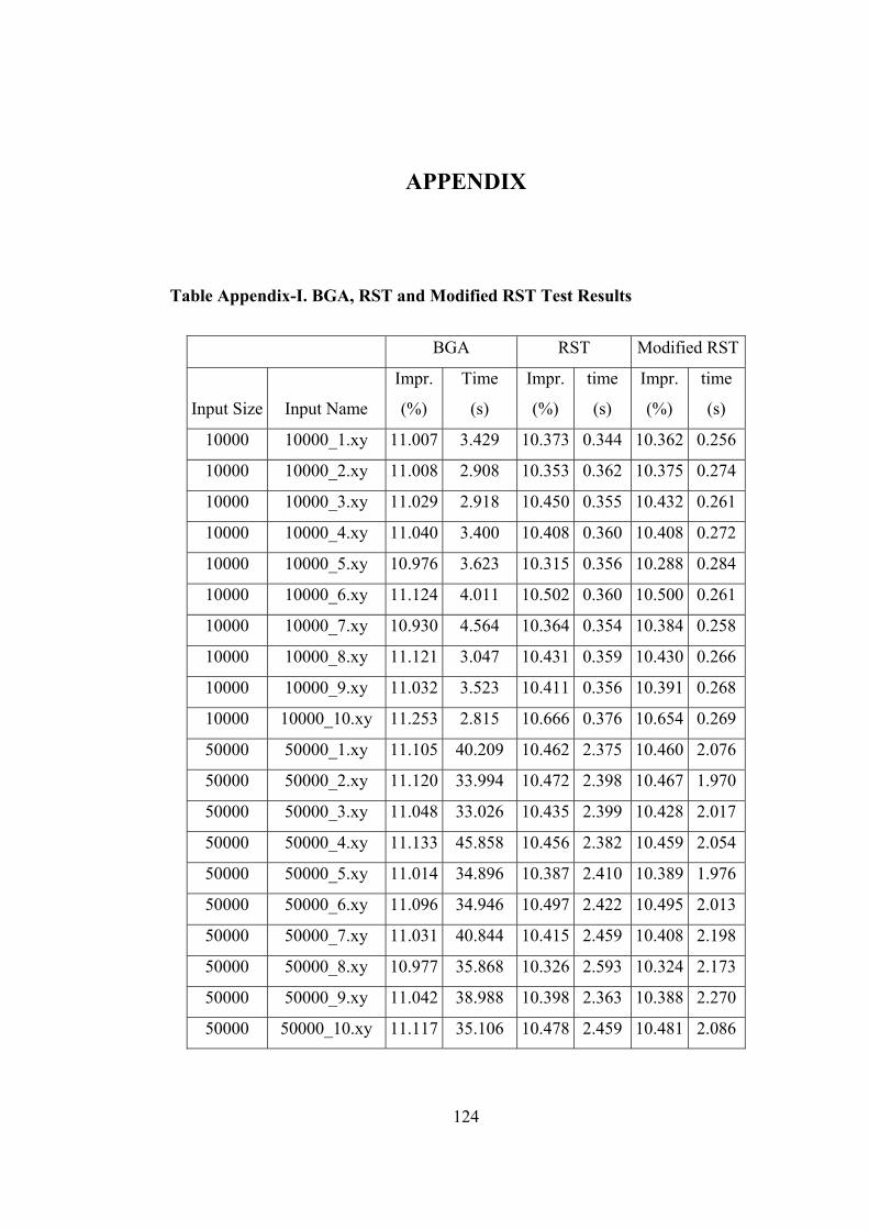
http://www.ph.surrey.ac.uk/~phs3ps/mpi-erwin-1.html

http://eternallyconfuzzled.com/tuts/andersson.html

124

APPENDIX

Table Appendix-I. BGA, RST and Modified RST Test Results


Input Size Input Name

Impr.

(%)

Time

(s)

Impr.

(%)

time

(s)

Impr.

(%)

time

(s)

10000 10000_1.xy 11.007 3.429 10.373 0.344 10.362 0.256

10000 10000_2.xy 11.008 2.908 10.353 0.362 10.375 0.274

10000 10000_3.xy 11.029 2.918 10.450 0.355 10.432 0.261

10000 10000_4.xy 11.040 3.400 10.408 0.360 10.408 0.272

10000 10000_5.xy 10.976 3.623 10.315 0.356 10.288 0.284

10000 10000_6.xy 11.124 4.011 10.502 0.360 10.500 0.261

10000 10000_7.xy 10.930 4.564 10.364 0.354 10.384 0.258

10000 10000_8.xy 11.121 3.047 10.431 0.359 10.430 0.266

10000 10000_9.xy 11.032 3.523 10.411 0.356 10.391 0.268

10000 10000_10.xy 11.253 2.815 10.666 0.376 10.654 0.269

50000 50000_1.xy 11.105 40.209 10.462 2.375 10.460 2.076

50000 50000_2.xy 11.120 33.994 10.472 2.398 10.467 1.970

50000 50000_3.xy 11.048 33.026 10.435 2.399 10.428 2.017

50000 50000_4.xy 11.133 45.858 10.456 2.382 10.459 2.054

50000 50000_5.xy 11.014 34.896 10.387 2.410 10.389 1.976

50000 50000_6.xy 11.096 34.946 10.497 2.422 10.495 2.013

50000 50000_7.xy 11.031 40.844 10.415 2.459 10.408 2.198

50000 50000_8.xy 10.977 35.868 10.326 2.593 10.324 2.173

50000 50000_9.xy 11.042 38.988 10.398 2.363 10.388 2.270

50000 50000_10.xy 11.117 35.106 10.478 2.459 10.481 2.086

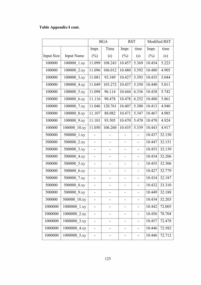
125

Table Appendix-I cont.



Impr.

(%)

Time

(s)

Impr.

(%)

time

(s)

Impr.

(%)

time

(s)

100000 100000_1.xy 11.099 108.243 10.457 5.369 10.454 5.223

100000 100000_2.xy 11.096 106.012 10.480 5.592 10.480 4.905

100000 100000_3.xy 11.081 93.349 10.427 5.393 10.435 5.044

100000 100000_4.xy 11.049 103.272 10.437 5.350 10.440 5.011

100000 100000_5.xy 11.098 96.114 10.444 6.336 10.438 5.742

100000 100000_6.xy 11.116 90.478 10.478 6.252 10.480 5.861

100000 100000_7.xy 11.046 120.761 10.407 5.380 10.413 4.940

100000 100000_8.xy 11.107 88.082 10.471 5.347 10.467 4.985

100000 100000_9.xy 11.101 93.505 10.470 5.470 10.470 4.924

100000 100000_10.xy 11.050 106.260 10.435 5.339 10.443 4.917

500000 500000_1.xy - - - - 10.437 32.150

500000 500000_2.xy - - - - 10.447 32.151

500000 500000_3.xy - - - - 10.453 32.139

500000 500000_4.xy - - - - 10.434 32.206

500000 500000_5.xy - - - - 10.455 32.306

500000 500000_6.xy - - - - 10.427 32.779

500000 500000_7.xy - - - - 10.434 32.187

500000 500000_8.xy - - - - 10.432 33.310

500000 500000_9.xy - - - - 10.449 32.188

500000 500000_10.xy - - - - 10.434 32.203

1000000 1000000_1.xy - - - - 10.442 72.005

1000000 1000000_2.xy - - - - 10.456 78.704

1000000 1000000_3.xy - - - - 10.457 72.478

1000000 1000000_4.xy - - - - 10.446 72.582

1000000 1000000_5.xy - - - - 10.446 72.712

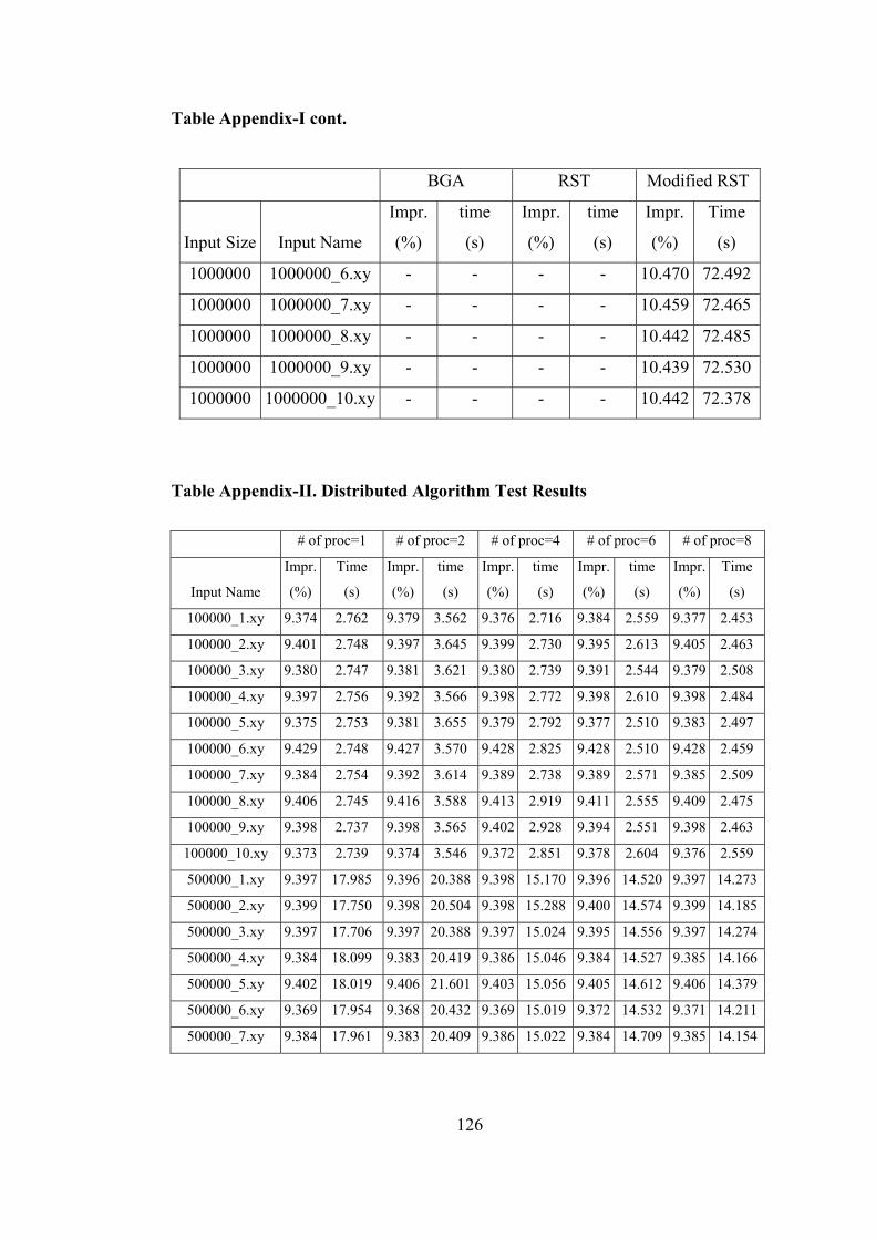
126

Table Appendix-I cont.



Impr.

(%)

time

(s)

Impr.

(%)

time

(s)

Impr.

(%)

Time

(s)

1000000 1000000_6.xy - - - - 10.470 72.492

1000000 1000000_7.xy - - - - 10.459 72.465

1000000 1000000_8.xy - - - - 10.442 72.485

1000000 1000000_9.xy - - - - 10.439 72.530

1000000 1000000_10.xy - - - - 10.442 72.378

Table Appendix-II. Distributed Algorithm Test Results


Input Name

Impr.

(%)

Time

(s)

Impr.

(%)

time

(s)

Impr.

(%)

time

(s)

Impr.

(%)

time

(s)

Impr.

(%)

Time

(s)

100000_1.xy 9.374 2.762 9.379 3.562 9.376 2.716 9.384 2.559 9.377 2.453

100000_2.xy 9.401 2.748 9.397 3.645 9.399 2.730 9.395 2.613 9.405 2.463

100000_3.xy 9.380 2.747 9.381 3.621 9.380 2.739 9.391 2.544 9.379 2.508

100000_4.xy 9.397 2.756 9.392 3.566 9.398 2.772 9.398 2.610 9.398 2.484

100000_5.xy 9.375 2.753 9.381 3.655 9.379 2.792 9.377 2.510 9.383 2.497

100000_6.xy 9.429 2.748 9.427 3.570 9.428 2.825 9.428 2.510 9.428 2.459

100000_7.xy 9.384 2.754 9.392 3.614 9.389 2.738 9.389 2.571 9.385 2.509

100000_8.xy 9.406 2.745 9.416 3.588 9.413 2.919 9.411 2.555 9.409 2.475

100000_9.xy 9.398 2.737 9.398 3.565 9.402 2.928 9.394 2.551 9.398 2.463

100000_10.xy 9.373 2.739 9.374 3.546 9.372 2.851 9.378 2.604 9.376 2.559

500000_1.xy 9.397 17.985 9.396 20.388 9.398 15.170 9.396 14.520 9.397 14.273

500000_2.xy 9.399 17.750 9.398 20.504 9.398 15.288 9.400 14.574 9.399 14.185

500000_3.xy 9.397 17.706 9.397 20.388 9.397 15.024 9.395 14.556 9.397 14.274

500000_4.xy 9.384 18.099 9.383 20.419 9.386 15.046 9.384 14.527 9.385 14.166

500000_5.xy 9.402 18.019 9.406 21.601 9.403 15.056 9.405 14.612 9.406 14.379

500000_6.xy 9.369 17.954 9.368 20.432 9.369 15.019 9.372 14.532 9.371 14.211

500000_7.xy 9.384 17.961 9.383 20.409 9.386 15.022 9.384 14.709 9.385 14.154

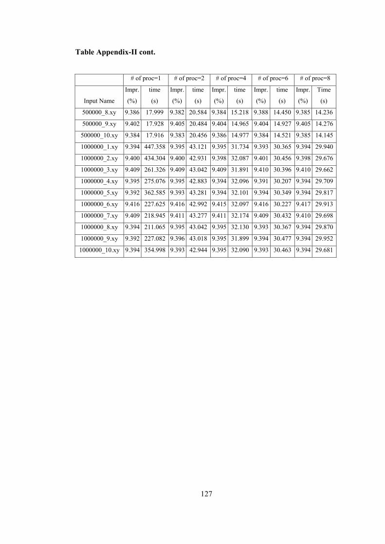
127

Table Appendix-II cont.


Input Name

Impr.

(%)

time

(s)

Impr.

(%)

time

(s)

Impr.

(%)

time

(s)

Impr.

(%)

time

(s)

Impr.

(%)

Time

(s)

500000_8.xy 9.386 17.999 9.382 20.584 9.384 15.218 9.388 14.450 9.385 14.236

500000_9.xy 9.402 17.928 9.405 20.484 9.404 14.965 9.404 14.927 9.405 14.276

500000_10.xy 9.384 17.916 9.383 20.456 9.386 14.977 9.384 14.521 9.385 14.145

1000000_1.xy 9.394 447.358 9.395 43.121 9.395 31.734 9.393 30.365 9.394 29.940

1000000_2.xy 9.400 434.304 9.400 42.931 9.398 32.087 9.401 30.456 9.398 29.676

1000000_3.xy 9.409 261.326 9.409 43.042 9.409 31.891 9.410 30.396 9.410 29.662

1000000_4.xy 9.395 275.076 9.395 42.883 9.394 32.096 9.391 30.207 9.394 29.709

1000000_5.xy 9.392 362.585 9.393 43.281 9.394 32.101 9.394 30.349 9.394 29.817

1000000_6.xy 9.416 227.625 9.416 42.992 9.415 32.097 9.416 30.227 9.417 29.913

1000000_7.xy 9.409 218.945 9.411 43.277 9.411 32.174 9.409 30.432 9.410 29.698

1000000_8.xy 9.394 211.065 9.395 43.042 9.395 32.130 9.393 30.367 9.394 29.870

1000000_9.xy 9.392 227.082 9.396 43.018 9.395 31.899 9.394 30.477 9.394 29.952

1000000_10.xy 9.394 354.998 9.393 42.944 9.395 32.090 9.393 30.463 9.394 29.681

sequential and parallel heuristic algorithms for the rectilinear...

Documents