sequential bottleneck decomposition: an … · 2008-12-14 · sequential bottleneck decomposition:...

SEQUENTIAL BOTTLENECK DECOMPOSITION: AN APPROXIMATION METHOD FOR GENERALIZED

JACKSON NETWORKS

J. G. DAI Georgia Institute of Technology, Atlanta, Georgia

VIEN NGUYEN Massachusetts Institute of Technology, Cambridge, Massachusetts

MARTIN 1. REIMAN AT&T Bell Laboratories, Murray Hill, New Jersey

(Received September 1991; revisions received April, October 1992; accepted December 1992)

In heavy traffic analysis of open queueing networks, processes of interest such as queue lengths and workload levels are generally approximated by a multidimensional reflected Brownian motion (RBM). Decomposition approximations, on the other hand, typically analyze stations in the network separately, treating each as a single queue with adjusted interarrival time distribution. We present a hybrid method for analyzing generalized Jackson networks that employs both decomposition approximation and heavy traffic theory: Stations in the network are partitioned into groups of "bottleneck subnetworks" that may have more than one station; the subnetworks then are analyzed "sequentially" with heavy traffic theory. Using the numerical method of J. G. Dai and J. M. Harrison for computing the stationary distribution of multidimensional RBMs, we compare the performance of this technique to other methods of approximation via some simulation studies. Our results suggest that this hybrid method generally performs better than other approximation techniques, including W. Whitt's QNA and J. M. Harrison and V. Nguyen's QNET.

nuestions related to the performance of computer, \/ communication, and manufacturing systems are ten addressed through the analysis of queueing network models. Exact solutions under realistic assumptions remain elusive, making approximate solutions a practical necessity. A popular approximation technique is decomposition, which consists of breaking the network into smaller pieces (typically with one station in each piece), and analyzing each piece separately. Examples of decomposition approximations are contained in Kuehn (1979), Whitt (1983), Bitran and Tirupati (1988), and Reiman (1990). All of these papers decompose the network into single stations. QNET, as described by Harrison and Nguyen (1990), is an alternative method for approximating queueing networks. Motivated by heavy traffic theory, QNET uses a reflected Brownian motion (RBM) on the J-dimensional nonnegative orthant to approximate a J-station queueing network. Numerical results can then be obtained using the procedure described in Dai and Harrison (1992),

known as the QNET algorithm. However, the computational complexity of the QNET algorithm grows in the size of the network, making it impractical for analyzing large networks.

The goal of this paper is to develop a hybrid method for approximating generalized Jackson networks using both decomposition methodology and heavy traffic theory. Our method, which we call Sequential Bottle- neck Decomposition (SBD), first partitions stations in the network into several "ordered" subnetworks (where each subnetwork may contain more than one station), then analyzes the subnetworks "sequentially" using a variant of the QNET method. This approximation is based on a heavy traffic limit theorem for queueing networks with several bottleneck stations (c.f. Johnson 1983, Chen and Mandelbaum 1991). When analyzing a particular subnetwork, SBD divides the remaining stations of the network into two sets, those that have larger traffic intensities than the stations in the designated subnetwork, and those with smaller traffic intensities. (This implies that

Subject classifications: Queues, networks: performance analysis of generalized Jackson networks. Probability, stochastic model applications: heavy traffic and Brownian system model.

Area of review: STOCHASTIC PROCESSES AND THEIR APPLICATIONS.

Operations Research 0030-364X/94/4201-01 19 $01.25 Vol. 42, No. 1, January-February 1994 119 ? 1994 Operations Research Society of America

120 / DAI, NGUYEN AND REIMAN

subnetworks are composed of stations whose traffic intensities are "roughly" similar.) Stations with smaller traffic intensities are treated as if their service times are zero (they are "instantaneous switches"). Stations with larger traffic intensities are treated as if they are supersaturated (or overloaded), which turns them into sinks for customers routed to them, and sources for customers routed from them. The analysis of a subnetwork with k stations is thus reduced to formulating the appropriate k-dimensional reflected Brownian motion, and then finding the stationary distribution of the RBM. Note that this method over- comes issues of computational complexity associated with the QNET method of Harrison and Nguyen because subnetworks can be kept to a reasonable size.

Reiman (1990) proposes two decomposition approximations for generalized Jackson networks which are similar in spirit to the SBD method described above. The critical difference in the methods proposed in Reiman (1990) is that all subnetworks are composed of a single station. The main incentive for using single-station subnetworks is that the approximating process, one-dimensional reflected Brownian motion, has a known (exponential) stationary distribution. The recent work of Dai and Harrison, which provides numerical solutions for the stationary distribution of multidimensional reflected Brownian motion on the nonnegative orthant, opens up the possibility of using bottleneck subnetworks of all sizes. The purpose of this paper is to explore the benefits of extending the methods first described in Reiman (1990) to subnetworks that consist of more than one station. To our knowledge, this is the first description of a decomposition approximation that makes use of multistation subnetworks for generalized Jackson networks.

The rest of the paper is organized as follows. We devote Section 1 to background material: In subsection 1.1 we present the details of the generalized Jackson network model; a general discussion of decomposition approximations is contained in subsection 1.2, and a description of the QNET method is provided in subsection 1.3. The sequential bottleneck decomposition (SBD) method is described in Section 2. In Section 3 we present some numerical results which compares the performance of SBD, QNET, and QNA (Whitt).

We conclude this section with a brief comment on our notation. All vectors are column vectors unless something is said to the contrary. For a J-vector a, if - C $1, 2, . . ., J}, then aB is the I Sl -vector (I -l is then cardinality of Sq) consisting of all elements of a with indices in _q. Similarly, if A is a J x J matrix,

then A, is the principal submatrix associated with indices in i5. Finally, givenf(l.) as a real-valued function and h as a constant, we will use the notation f(t) ht to mean f(t)/t h as t -> oo. In the case thatf(.) is a vector (matrix) valued function and h is a vector (matrix), one interpretsf(t) ~ ht component- wise in the natural way.

1. PRELIMINARIES

1.1. The Generalized Jackson Network

The queueing network we consider has J single-server stations, each of which has an associated infinite capacity waiting room. At least one station has an arrival stream from outside the network, and the arrival streams are assumed to be mutually independent renewal processes. The arrival rate to station i is ai, and the interarrival variance is a;, 1 < i < J. The squared coefficient of variation (SCV) for arrival stream i, ci,i, is Cai. Since our approximations are based on two moments, that is all we define. Cus- tomers are served in a first-in, first-out order at each station. Service times at stations 1, ..., J form mutually independent sequences of i.i.d. random vari- ables. The mean service time at station i is ri, and the service time variance is si2, 1 < i < J. The squared coefficient of variation of service times at station i, ci, is rT2si. After completing service at station i, a customer is routed to station j with probability Pij, 1 s j < J, and out of the network with probability 1 -

V- PFj, 1 < i s J. We assume that the network is open, so all customers eventually leave. This is true if the matrix P = (Pij) is strictly substochastic. We further assume that arrival streams, service streams, and routing streams are independent. We define the traffic intensity exactly as in Jackson (1957). Let X be the unique solution of

X = a + P'X, (1)

where a = (a,, a2, . . ., aj)'. By our assumption on P, (1) has a unique solution given by X = (I - P')-la =

Q'a, where Q = Xn=O JJPf. The traffic intensity at station i, pi, is given by

pi = X1T, 1 < i < J. (2)

Under certain technical assumptions, Borovkov (1986) has shown that this network is ergodic if

pi <1,I<.i < J. (3)

1.2. Decomposition Approximations

In decomposition approximation techniques, the analysis of a network is separated into analyses of

DAI, NGUYEN AND REIMAN / 121

smaller subnetworks, each typically consisting of one station. The mean waiting time of each station is then approximated by an expression that is similar in form to the approximation of Kraemer and Lagenbach-Belz (1976) for the GI/G/1 queue. In particular, let w

denote the approximation for the mean steady-state waiting time at station j under approximation scheme x. The typical decomposition approximation has the form

i( pi) 2 (4)

where Cjf is an approximate measure under scheme x of the composite variability associated with station j. One can think of CJ as being the sum of two components: The first component is associated with the SCV of the service time distribution, and the second component is associated with the SCV of the arrival process to that station. It is the expression for Cjx that differentiates the various decomposition approximations and determines their effectiveness and accuracy. Observe that in the special case of Jackson networks (i.e., networks of the type considered here with the additional assumption that all distributions are exponential), the exact answer is obtained by setting CJackson = 2 for all stations j.

One example of a decomposition approximation is Whitt's Queueing Network Analyzer (QNA) (Whitt 1983). The expression for the waiting time at each station is of the same form as (4); however, the determination of CV,A is rather involved, so we do not discuss it here and refer the interested reader to Whitt for details. Other decomposition approximations are contained in Kuehn (1979) and Bitran and Tirupati (1988).

The approximation for total mean sojourn time in the network is easy to derive from estimates of mean waiting times. Let vj denote the mean total number of visits that a customer makes to station j; it follows from the definition of the routing matrix P that if the customer in question enters the network through station i, then Vj = [(I - P)-']ij. The decompositon approximation scheme x estimates the mean steady- state sojourn time SI by

J SX = vA I ;x + rj]. (5)

j=1

1.3. The QNET Method

To use the QNET method (Harrison and Nguyen), one first replaces the queueing network by what we

call an approximating Brownian system model. For generalized Jackson networks considered in this paper, this step is rigorously justified by the limit theorem of Reiman (1984). The second step is the computation of the stationary distribution for the Brownian model, which amounts to solving a certain highly structured partial differential equation. No closed-form solution to the partial differential equation is known for the general case; however, an algorithm has been devel- oped by Dai and Harrison to numerically solve for the stationary distribution.

We begin by deriving the parameters for the Brownian model from the "primitive data" associated with the generalized Jackson network. The development here closely follows that of Harrison and Nguyen, and the interested reader is referred there for a more detailed description. First, set

6= p - e, (6)

where p is the vector of traffilc intensities calculated in (2) and e is the J-dimensional vector of ones. The jth element of 0 can be interpreted as the rate at which work accumulates at station j if the server is always busy. The stability condition (3) is equivalent to requiring 0 < 0; that is, on average, work accumulates at a negative rate.

Next let T be the diagonal matrix with diagonal elements (r,, . . ., rj), and define

M = T(I - P)-l T-1. (7)

It follows from the previous interpretation of the matrix (I - P')-' that Mij represents the average amount of residual work for server i embodied in a unit of immediate work for server j. The matrix M contains all the information about customer routing that is required in the QNET approach to system performance analysis. Observe that the "routing matrix" M is invertible, and denote its inverse by R,

R =M-1 = T(I-P')T-'. (8)

The final parameter of the Brownian system model is a covariance matrix F associated with the "workload input" processes to the network. For a more explicit definition of r, some additional notation must be introduced. Let Ej(t) be the number of external arrivals to enter station j by time t; let Aj(t) be the total number of visits to station j made by those customers who enter the network by time t (regardless of where the customer enters the network); and let E(t), A(t) be the J-dimensional vector processes defined in the obvious way. Let { w/(1), wj(2), . . .} be a sequence of i.i.d. service times at station j. We are interested in obtaining the asymptotic covariance


matrix IF associated with the total load input process L(t) = (L,(t), . .. , L,(t))' defined by

Lj(t) = w(1) + ... + wj(Aj(t)). (9)

Let 1k'(1), k1(2), ...) be a sequence of i.i.d. routing vectors for customers completing services at station l; the jth component of the vector equals one if the customer goes next to station j, and all other components are zero. Denoting by q5 a generic element of this sequence, it follows that

E[q/] = Pf' and Cov[k'] = H', (10)

where P, is the lth row of the routing matrix P and H' is the J x J matrix defined by

Hj= _PPz i

=1J H' -Pl F,,) oi

Next define the J-dimensional cumulative sums and the centered processes

n n

=bl(n) = E 5+(k) and 4'(n) = (0'(k) - PI ). k=l k=l

One can now define the total arrival process A(t) in terms of external arrival processes and routing vectors by means of the representation

J

A(t) = E(t) + E 4'(A,(t)) 1=1

J

= E(t) + , 4(Ai(t)) + P'A(t). ( 1) 1=1

The obvious manipulations reduce the above expression to

A(t) = (I - P1)- l E(t) + E V(A(t))] (12)

From renewal theory and the assumed independence of the various external arrival processes, one has E[E(t)] - at and Cov[E(t)] - At, where

A = diag(acY,1, .. . c a2,J). (13)

Furthermore, because the random vectors 1" have zero means, we can show that the asymptotic covariance matrix of the bracketed quantity in (12) remains unchanged if one replaces A,(t) by its asymptotic mean X,t, or more precisely, by the integer part of X,t. Com- bining that fact with (10), (13), and the obvious independence properties, one has from (12) that Cov[A(t)] - Bt, where

B = [(I - P')-l](A + H)[(I - P')-']' (14a)

and J

H= X X1H'. (14b) 1=1

The service times wj(n) are independent of A(t), so it follows from (9) and (14) that Cov[L(t)] rt, where

F= TBT+ TDT, (15)

and D = diag(X1c , ... c Xjc'J). Substituting (14) into (15) and simplifying, one has

F = [T(I - P')-']G[T(I - P')-']', (16)

where

G = A + H + (I - P')D(I-P). (17)

Readers may verify that (17) is equivalent to

aci + X1cS( 1 -2P'')

+ '[EJn=i XMPmi(PmzC2m + 1 -Pmi)] i =

Gj _ic2,p-jc2jPji

J=X AM(1 - C2m)PmzPmj ip mJ.

(18)

The approximating Brownian system model is defined by these six relationships:

Z(t = W() + I(t) (19)

{1(t), t - 0} is a J-dimensional Brownian motion with drift vector 0 and covariance matrix P, (20)

I(.) is nondecreasing and continuous with I(0) = 0 (21)

Ij(.) increases only when Wj((.) = 0, (22)

Z(t) = MW(t), and (23)

W(t) 3 0. (24)

The process W(t) as defined by (19)-(24) is a J-dimensional reflected Brownian motion with drift vector ,u = RO, covariance matrix Q = RrR' = TGT', and reflection matrix R, or simply (,A, Q, R) RBM. If pj < 1 for each stationj, Harrison and Williams (1987) proved that W(t) converges in distribution to a random vector W* = (W*, ..., W*) as t -4 oo. The QNET method proposes that H* be used as the approximating steady-state workload vector for the queueing network. Observe that a rigorous justification of this approximation requires an interchange of limits; namely, it remains to be shown that the steady-state distribution of the limiting Brownian model well approximates the heavy-traffic limit of the original queueing network in steady state.

DAIT NGUYEN AND REIMAN / 123

Nevertheless, we will proceed as if this were true, and set

W{yNET = E(Wj*) j = 1, ...,J. (25)

Finally, given the steady-state distribution of the waiting vector, QNET approximates the mean steady-state sojourn time via an equation of the same form as (5).

Let ir be the distribution of the limiting random variable V". Before we state an analytical characterization of the limiting distribution ir, we first introduce some additional notation. Let S denote the J-dimensional nonnegative orthant (the state space of the process), and let

Fj= {(xI,. . . ,x)ES:xj=01, forj= 1,. . .,J.

Recall that A, Q, and R are the drift vector, covariance matrix, and reflection matrix associated with W, and define the corresponding second-order elliptic differential operator CV via

1' J J 2 J

Wf(x) = 2 EE Qi d f(x) + EX d f(x), 2 i=l j=l axaj )j= Xj

f E C2(S),

where CQ(S) is the set of functions, which together with their first and second derivatives are continuous and bounded on S. Next, for each j = 1, . .. , J, define the directional derivative -7jf(x) = Ri Vf(x), where Ri is the jth column of the reflection matrix R. Note that -, f is the directional derivative off in the direc- tion of reflection associated with boundary face Fj.

Harrison and Williams prove that the stationary distribution ir has a density function po, which together with a certain boundary density function pj on Fj(j = 1, ..., J) jointly satisfy the basic adjoint relationship (BAR):

f S?f(x).po(x) dx + - E r % f(x) pj(x) daj = 0,

fE Ct(S); (26) here, rj is Lebesgue measure on boundary face F1(j = I I... ., J).

Dai and Harrison describe a general algorithm for the numerical solution of the basic adjoint relationship (26). There are some choices one has to make associated with that algorithm, and they have suggested one possibility. With that particular choice, the algorithm has been implemented in a computer program tenta- tively called QNET. Readers are referred to Dai (1990) and Dai and Harrison (1992) for a complete description of the algorithm as well as details of the implementation. Suffice it to say that QNET produces approximate densities indexed by n = 1, 2, ... of

the form pS')(x) = r ()(x). q(x), where r(n)(x) is some (n - 1)-degree polynomial of xl, . x. , J and

q(x) = exp (- 2,yj(l - Pj)[QIjJxj)

with -yj defined as

y --R-'y = e - p > O. (27)

Here e is the vector of ones. Under the condition

f [pO(x)2q(x) dx < oo and s (28)

T [pj(x)]2q(x) doj < oo,

the algorithm converges in the sense that

T [p n)(X) _ po(X)]2q(x) dx -- 0 as n -? oo. (29)

Unfortunately, not all RBMs arising from queueing networks satisfy condition (28), so convergence in the sense of (29) is not guaranteed in general. It is conjec- tured in Dai and Harrison that p() converges to po in some weak sense even if condition (28) is not satisfied. Numerical experiences so far seem to support this conjecture. One expects that larger values of n will give better accuracy; but readers should be warned that numerical round-off errors might destroy the property. As a practical matter we have found that n = 4, 5, 6 generally gives satisfactory answers for the test problems examined thus far. If one fixes n = 5, the computational complexity of the algorithm is O(J'?), which means that small and medium sized problems can be solved relatively fast using the current implementation of the algorithm. As discussed above, the sequential bottleneck decomposition method devel- oped in this paper will eliminate the restriction of QNET on the size of networks.

2. THE SEQUENTIAL BOTTLENECK DECOMPOSITION (SBD)

2.1. Heavy-Traffic Limit of a Queueing Network With Bottlenecks

To motivate the SBD method, we first describe the heavy traffic behavior of a queueing network in which there are nonbottlenecks, defined as stations j with pj < 1; bottlenecks, stations j with pj = 1; and strict bottlenecks, stationsj with pj > 1. We will interchange- ably refer to the nonbottlenecks, bottlenecks, and strict bottlenecks as underloaded, balanced, and overloaded stations, respectively. Let ? denote the set of


stations that are underloaded, iw the set of balanced stations, and -e the set of overloaded stations.

The heavy traffic limit theorem of Chen and Mandelbaum states that under "heavy-traffic normal- ization," workload and queue length processes at all underloaded stations "vanish." Furthermore, the heavy traffic limit for the rest of the network is iden- tical to that for the system in which all underloaded stations have zero service times. Next, the limits for the queue length and workload processes at strict bottleneck stations require centering; that is, workload processes and queue length processes at these stations build up at a positive rate. Thus, one may think of these stations as having infinite queue lengths in steady state. Finally, the limit of the balanced subnetwork 5 is a I 'lj -dimensional reflected Brownian motion, whose parameters reflect the effects on g

from the nonbottleneck as well as strict-bottleneck stations.

Although we are interested only in networks whose stations have traffic intensities strictly less than one, and the work of Chen and Mandelbaum applies to networks containing traffic intensities that are greater than or equal to one, their theory provides the motivation for the sequential bottleneck decomposition method. In particular, it suggests the following mode of analysis: One can partition a network into several subnetworks of stations whose traffic intensities are approximately equal, and then analyze each subnetwork separately. To analyze a particular subnetwork, one treats the designated subnetwork as "balanced." All stations with lower traffic intensities than the stations in the designated subnetwork are treated as ";underloaded," and all stations with higher traffic intensities are viewed as "overloaded." Then, in the spirit of the Chen and Mandelbaum theory, analysis of the designated subnetwork reduces to formulating an appropriate Brownian system model, and then calculating the steady-state distribution of the associated RBM.

2.2. The Mechanics of SBD Without loss of generality, one can assume stations are numbered so that Pi < P2 < . .. pJ < 1. Consider a partition that divides the J stations into N subsets, indexed by n = 1, ..., N. The nth subset will be referred to as subnetwork S, Suppose that partitions are made in such a way that all stations in a subnetwork are more or less balanced; that is, their traffic intensities are in the same range. We will further assume that the subnetworks Sl, . . ., SN are ordered in the following sense: if m < n, then pi < pj for all stations i E Sm and j E Sn. Observe that we have not

specified the number of subsets N, nor how the partition is to be made. For now let us proceed assuming that such a partition has already been made. In Section 3, we present some numerical examples and suggest "'natural" partitions for these networks. However, we do not strive to provide a general prescription for decomposing a network.

The SBD method analyzes the queueing network by analyzing each of the subnetworks S, ..., SN separately. The remainder of this section is devoted to specifying how to analyze a subnetwork S". Relative to S, all stations in subnetworks S with I < n are less heavily loaded, and similarly, all stations in subnetworks Sm with m > n are more heavily loaded. Thus, from the point of view of S, the network can be decomposed into three components, the "balanced" subnetwork q(n) = S, the "underloaded" subnetwork 1?(n) = Um<nSm, and the "overloaded" subnetwork ie(n) = Um>nSm. In the spirit of the limit theorem by Chen and Mandelbaum, all stations in JX(n) will be treated as if they are supersaturated, while all stations in ck<(n) are instantaneous switches (i.e., stations with zero service times). A supersaturated station has two main characteristics which result from it having an infinite queue length. First, customers routed there never return, and second, departures from there form a renewal process because the server is always busy.

To analyze subnetwork Sn one needs to define the parameters associated with the subnetwork, namely, the "exogenous" interarrival time distributions, the service time distributions, as well as the routing of the customers within the subnetwork. To minimize notation, henceforth S, q, 9i, and -.&will be used to mean S,, s?(n), and X6(n), respectively. We begin with the computation of the internal routing probabilities associated with subnetwork S. Let P = (Pij) be a J x J matrix whose components are given by

PiJ = { (30)

By assumption, P is a strictly substochastic matrix; from the construction in (30), it is easy to verify that P is also a strictly substochastic matrix, hence one can set

Q = (I _ p)- l (31)

For i E E and j E E U &, Qij denotes the probability that when a customer at station i first leaves the underloaded subnetwork @, it enters the nonunder- loaded subnetwork n U -e via station j. Next,


defining

P1i = P1i + E Pi,Q4y, (32) le 9i

it follows from the interpretation of Q that P is the internal routing matrix for the bottleneck subnetwork S; that is, for i, j E q, Pij is the probability that a customer at station i first re-enters the bottleneck subnetwork through station j. Similarly, P5 is the routing matrix to the balanced subnetwork for customers departing from the overloaded subnetwork. Finally, it is not difficult to verify that P, is strictly substochastic, and we set

QrgO_iO = (I - P_)l. (33)

The next step in the analysis is the determination of the "exogenous" arrival processes to the balanced subnetwork. The arrival process to each station j E E

is a superposition of several renewal processes, which can be identified as emanating from three sources:

a. the exogenous arrival stream of the original queueing network;

b. exogenous arrival streams to the underloaded stations which are then routed directly to j; and

c. arrivals resulting from the renewal services of stations that are supersaturated. (34)

In the exposition below, it will be convenient to introduce the following enumeration scheme. We will be concerned with vectors, matrices, and processes that are restricted to stations in the balanced subnetwork ?. Strictly speaking, the stations in - will not be numbered consecutively by 1, . . ., I l, but for the sake of notational simplicity, we abuse terminology somewhat and refer to stations in n by indices 1, . . ., 1-41, where by "station" j we mean the jth element in the set -4.

As in the development of subsection 1.3, let us now define sequences of i.i.d. routing vectors {?Q(1), ok(2), . . .} and o- k(2), . . .} for k E i, / E E U 9, corresponding to the routing matrices Q and P, respectively. To be more specific, denoting by OQ a generic element of the sequence {?k(1), ok(2), ...}, and by k' a generic element of {10(1), +/(2), ... , ok (respectively, 14) is a 1-5eI-vector whose jth component equals unity if a customer in k E @? (respectively, / E X&) next enters the balanced subnetwork g via station j, and all other components are zero. (Note that the new enumeration scheme of stations in -7 is being used here.) It thus follows that

E[OQ] = QLk Cov[OQ] = Hk, k E = (35)

E[01-] = P, Cov[op] = Hp, / E E U 4 (36)

where Qke is the kth row of Q P, is the lth row of P.,e and HQ, H^ are x I x f/I matrices defined by

(HQ) i = Qk_ - Q i (37)

LQkiQkJ 1?1,~

( =P'i(AlA Pli) i = j =H {"=j"p 71 (38)

Next, define cIQ and 4%^ to be the associated cumulative sums processes,

n n

(bQ(n)= E 0b(m) and o'^(n) E 0^(m) m=l m=1

and also their centered versions, n

4k (n) = E kbQ(m) - QLk] m=l

and n

4P^(n) = E kb'(m) - P,]. m=1

Using this representation, the modified external arrivals to the balanced subnetwork, denoted as the 14 -vector E, can now be expressed as a sum of the three sources of arrivals enumerated in (34). Let Si(t), i E e be a renewal process with rate Xi and SCV c2j. One can interpret Si(t) as the renewal process associated with services from station i with the following modification. We substitute the throughput rate Xi for the service rate at station i (originally r-'), as we believe that this more accurately represents the dynamics of the system. Then

E(t) = Ee(t) + E k (Ek(t)) + E (SXt)) keG2 Ief

= E(t) + Q 'E(t) + P?S4)

+ E 4 (EJ(t)) + E 4 (S1(t)) (39) ke %/ Iei

Notice that the last two terms of (39) consist of zero- mean random vectors. Hence, their asymptotic covariance matrix remains unchanged if Ek(t) and S,(t) were replaced by the asymptotic means, akt and x1t, respectively. From (35)-(39) and the independence assumptions, it follows that E[E(t)] & at and Cov[E(t)] At, where

A= + Q % a + P 9Xe (40)

and

[aiCa,i + LXe=. a!kOQki(QkiCa,k + 1 Qki)

) + Z, X P11i( 1c',1 + 1 - P,i) i = j

- Ek e, ak(l Ca,k)QkiQkj

- E l ,,21 ' 'A

i {


Finally, imitating the development of (11 )-(14), the modified total arrival process to the balanced subnetwork - can now be expressed as

A( = (I - PW)' E(t) + E kp(Ai(t)) iE- O

=Ql (k[() p(Ai(t))] (42) iE=-_~

Furthermore, the process A(t) has asymptotic mean X and covariance matrix B given by

X = (I - P') a =Qa (43)

and

B = QieAA + H]Qe, H= E X,(HP^),_ (44) 1E-2

where Qi,, Hp, &, and A are given in (33), (38), and (40)-(4 1).

Because service times are not affected in the decomposition, the modified total load input processes to the balanced subnetwork q, denoted by L(t), retain the same representation of (9),

Lj(t) = wi(l) + ... + wj(Aj(t)).

From the above expression and (1 5)-(18), the asymptotic covariance matrix r of L has the form

r = ( TQ W)G( Q 9),(45)

with

G = A + H + (I - P (I - RPe9~e), (46)

and D = diag( Xc i, i E ). Algebraic manipulations show G to have the components:

aica ci + XicSi( 1 - 2P1i)

+ Eke% akQki(QkiCa,k + 1 Qki)

+ S Cs2 + 1 - P,i)

G= + EE, XiPi(Piics2 + 1 - P1i) i = j (47)

- xiCs,iPii - X1CSJP1i - Xke% ak( l - ca,k)QkiQkJ

-_~ X,( 1 - cs, PiPj

- SE AX( 1 - Cs2,)P1Pj1 i ? i.

Defining

pj = X1r1, (48)

the bottleneck subnetwork n is approximated by a

I -I -dimensional RBM with parameters

4 = R(j - e),

Q = RrR' = T?q?qGT, and

R = T(I - P )T-7. (49)

This completes the description of the SBD method.

2.3. The Jackson Network

A typical validity test for an approximation method is to verify that it gives the correct solution for the class of Jackson networks. Recall that for such networks, the mean steady-state waiting time at each station is given by

WJackson = TiPi (50) j - pj

(0

In this subsection we show that SBD yields the approximations shown in (50) when applied to Jackson networks.

In Jackson networks, all service times and interarrival times are exponentially distributed, hence, C2 = C2 = 1 for allj = 1, J. Expression (47) for Gij thus simplifies to

|a ai + Xi(I 2Pij) + Ekc= akQki

Gii = + D, xP,i + ? x,P,i i =

l - ij -jji i ?1. (51)

Recall that ce = (I - P )X, so for each i E q, Xkei XkPki = Xi - ai. By definition, ai = ai + XkE akQki + D X1P,i, so (51) reduces to

{2Xj1= - (52)

One can verify that with these data, the skew symmetry condition in Harrison and Williams holds, which implies that the waiting times are exponentially distributed with mean

WBD =(I - ̂ X)(1 - Pi) -I ^ P

To prove the equivalence of (50) and (53), it suffices to show that for all i E q, Xi = Xi. The throughput rates X of the bottleneck subnetwork S uniquely satisfy (43), where 'a is given by (40). From (32), the internal routing matrix has the form P. = P. + P. ?Q, Substituting this expression and (40) into (43), we obtain

(I- Pg)3= a + P_gAe

+ Q ?4a+ Pj A] (54)


Recall the traffic equation

X = a + P'X, (55)

which has the unique solution given by X = (I -

P')-'a. In particular, we have

X Gi = a G + P ? + P GCX + P &X.

Using this expression in (54), we have

(I- Pn)X= a+ <X

+Q (-X -~~. (56) + [ ( I P, P G) X Gtp PG

It is straightforward to verify that (I- P- )QG?@=

PG,,, so that (56) reduces to

(I - Pw)S = a~ + P"X @ +P

+ P>AX,5- P X?. (57)

Again, because X uniquely solves the traffic equations (55), it satisfies

X = age + P'igA + P + P

so (57) becomes

(I - P")S = (I - P) .

Because (I - P ) is invertible, X = X?q and we have shown that WVSBD = WJackson

2.4. Some Notes on Choosing a Decomposition

We have completed the description of our approximation method for single-class open networks, based on a decomposition of the original system into smaller subnetworks. We will demonstrate the use of this method in the next section, where we will compare its performance with several other approximation schemes. As told, however, our story is not complete. To speak of the sequential bottleneck decomposition, we need to provide a more explicit prescription for breaking the original network into subnetworks. At present, it is not possible to recommend the "best" decomposition for a general case. On the other hand, we are able to suggest some basic guidelines.

First, one must construct subnetworks in such a way that the group of subnetworks can be ordered. That is, all traffic intensities of the stations within a subnetwork must be either smaller or greater than all traffic intensities in another subnetwork.

Second, noting that the decomposition method is partly driven by the dimensional limitations of Dai and Harrison's algorithm, we recommend that subnetworks be kept to a "reasonable" size. For example, based on the current implementation of their algorithm on a SUN SPARCstation 1, it takes 31.9 seconds

to analyze a five-station subnetwork, whereas it takes 2654.8 seconds to analyze an eight-station subnetwork. Therefore, for this computational platform, it is probably wise to decompose a network into subnetworks with five or less stations.

Third, the motivation for our decomposition technique derives partly from theoretical findings regard- ing the behavior of networks with nonbottlenecks, bottlenecks, and strict bottlenecks. Analogous to such a characterization, a default partition is to place the stations of a network into three groups: those that are lightly loaded, medium loaded, or heavily loaded. Our experience indicates that stations with traffic intensities greater than 0.85 may be regarded as heavily loaded; stations with traffic intensities less than 0.4 may be considered lightly loaded; and the remaining values correspond to the medium range of traffic intensities. If the default partition results in subnetworks that violate the size guidelines above, then these subnetworks should be decomposed further.

Of course, these are only general guidelines and the final decomposition must take into consideration the special circumstances of the network. For some networks, there will be an "obvious" decomposition, while the partition may be more vague in other situ- ations. For example, given a network of six queues whose traffic intensities are between 0.85 and 0.95, it is not clear that there would be a "best" decomposition, or that the network should be decomposed at all. In such a case, we suggest that the modeler experiment with different partitions and examine the range of results. As the figures in our next section suggest, however, this decomposition method is quite robust in the sense that one can typically expect similar approximations even with different partition schemes (provided, of course, that one abides by the rules for constructing subnetworks specified in subsection 2.2).

3. NUMERICAL EXAMPLES

3.1. A Three-Station Network

Pictured in Figure 1 is a three-station generalized Jackson network, where customers arrive to station 1 according to a Poisson process with rate a = 0.225. Customers who complete service at station 1 proceed to station 2, and after being served there go to either station 3 or to station 1, each with probability 1/2.

Customers finishing service at station 3 either go to station 2 or exit the system, each with probability 1/2.

The service-time distribution at station i is assumed to be general with SCV C2,. We consider five versions of this network. Each version corresponds to a


1/2

1/2

1 ~ ~ ~~~~~ 3

(X=0.225 1 1/2 1/2

Figure 1. A three-station network.

different triad of SCVs (c,1, cS,2, C3,3) chosen from the set: (0.0, 0.0, 0.0), (2.25, 0.0, 0.25), (0.25, 0.25, 2.25), (0.0, 2.25, 2.25), and (8.0, 8.0, 0.25). We label these five versions as systems A, B, C, D, and E. In each system we consider four different cases, which differ by the mean service times at each station. The parameters of these four cases are given in Table I.

Table I Mean Service Times of Four Cases of the

Three-Station Network Case ri 72 73 PI P2 P3

1 1 1 1 0.675 0.900 0.450 2 4/3 3/4 2 0.900 0.675 0.900 3 4/3 3/4 1 0.900 0.675 0.450 4 4/3 3/4 3/2 0.900 0.675 0.675

Table II gives the simulation estimates and approximations of the total mean sojourn time (calculated from (5)) in the network. Table III gives the mean sojourn time (service time plus waiting time) at each station for system D. In simulations, service times are fitted with Erlang distributions, exponential distributions, or hyperexponential distributions with balanced means depending on the SCV being less than one, equal to one, or larger than one, respectively. A random variable is said to have hyperexponential distribution with balanced means (having mean m and SCV c2 > 1) if it has density function

f(t) = pmle-"lt + (1 - p)12e-"2t, t : 0,

where p = 1/2 + 1/2 V(c2 - )/(c2 + 1), ALl = 2p/m and 82= 2(1 - p)/m. The simulations were performed using Panacea 3.3. 1. In all cases, ten replications were run and the simulation time of each replication was 1 05. In this table, as in all subsequent tables, the numbers in parentheses after the simulation results represent the half-width of 95 % confidence intervals, expressed as a percentage of the simulation average. The numbers in parentheses after the approximations represent percentage errors from the simulation average. This format makes it easy to determine the

Table II Simulation Estimates and Approximations for the Total Mean Sojourn Time of

the Three-Station Network System/Case Simulation QNA QNET (n = 5) SBD (n = 5)

A 1 40.390 (3.75%) 20.519 (-49.20%) * (****) 42.986 (6.43%) 2 59.580 (3.29%) 36.039 (-39.51%) 56.679 (-4.87%) 58.175 (-2.36%) 3 40.720 (4.78%) 23.985 (-41.10%) 38.682 (-5.00%) 40.188 (-1.31%) 4 42.119 (3.36%) 26.221 (-37.75%) 41.808 (-0.74%) 42.655 (1.27%)

B 1 52.399 (2.64%) 42.020 (-19.81%) 52.613 (0.41%) 50.200 (-4.20%) 2 91.523 (3.77%) 94.050 (2.76%) 83.704 (-8.54%) 95.270 (4.09%) 3 61.680 (3.44%) 72.230 (17.10%) 61.941 (0.42%) 60.902 (-1.26%) 4 63.336 (2.83%) 75.821 (19.71%) 64.142 (1.27%) 64.691 (2.14%)

C 1 44.244 (1.96%) 31.298 (-29.26%) 37.031 (-16.30%) 47.092 (6.44%) 2 92.417 (4.23%) 87.443 (-5.38%) 91.169 (-1.35%) 91.648 (-0.83%) 3 44.263 (4.69%) 33.222 (-24.94%) 43.966 (-0.67%) 44.994 (1.65%) 4 50.202 (1.04%) 41.353 (-17.63%) 51.077 (1.74%) 52.227 (4.03%)

D 1 55.813 (2.58%) 71.417 (27.96%) 58.754 (5.27%) 58.209 (4.29%) 2 98.364 (1.82%) 101.710 (3.40%) 97.198 (-1.19%) 94.363 (-4.07%) 3 47.718 (2.51%) 40.215 (-15.72%) 47.820 (0.21%) 48.206 (1.02%) 4 55.237 (4.37%) 49.281 (-10.78%) 55.990 (1.36%) 56.739 (2.72%)

E 1 134.426 (4.77%) 265.110 (97.22%) 155.080 (15.36%) 115.694 (-13.93%) 2 213.101 (3.47%) 308.440 (44.74%) 228.248 (7.11%) 206.114 (-3.28%) 3 138.722 (3.97%) 243.750 (75.71%) 161.290 (16.27%) 135.280 (-2.48%) 4 155.054 (4.37%) 252.330 (62.74%) 167.831 (8.24%) 147.299 (-5.00%)

Average absolute percentage error 32.12% 5.07% 3.64%


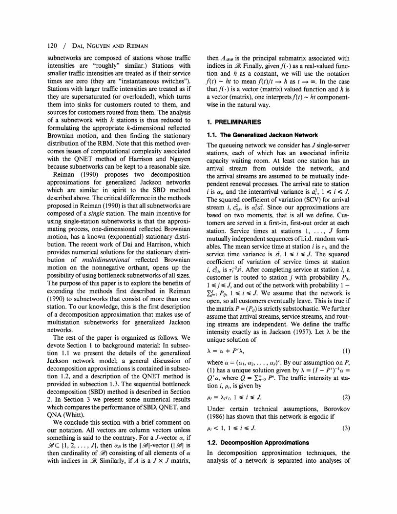
statistical significance of the errors. The QNA column contains the estimates produced by Whitt's QNA soft- ware package (Whitt). The QNET column contains the estimates obtained by the QNET method, as described in subsection 1.3. The SBD estimates are in the SBD column. In each table, we also display the average absolute percentage error of each approximation scheme, which is calculated by taking the average of the absolute value of the percentage errors.

The next paragraph gives a detailed discussion on how we partitioned the network into subnetworks when using the SBD method for this particular network. From Table II it is evident that both QNET and SBD outperform QNA, with SBD slightly better than QNET in general. For case 1 of system A, the current implementation of the QNET algorithm fails to con- verge to a positive number. We believe that (28) is not satisfied in this case, but further investigation of the QNET algorithm is needed to determine the exact cause of the problem.

In applying the sequential bottleneck decomposition method, we partitioned the network as follows. For case 1, we use the partition SI = 11, 3}, and S2 =

12). Similarly, for case 3, we consider the grouping SI = 12, 31 and S2 = {l}. In case 2, stations 1 and 3 have the same traffic intensity, so we set SI - 12}, and S2 = {1, 3}. Finally, for case 4, we have SI = 12, 3}, and S2= 11}.

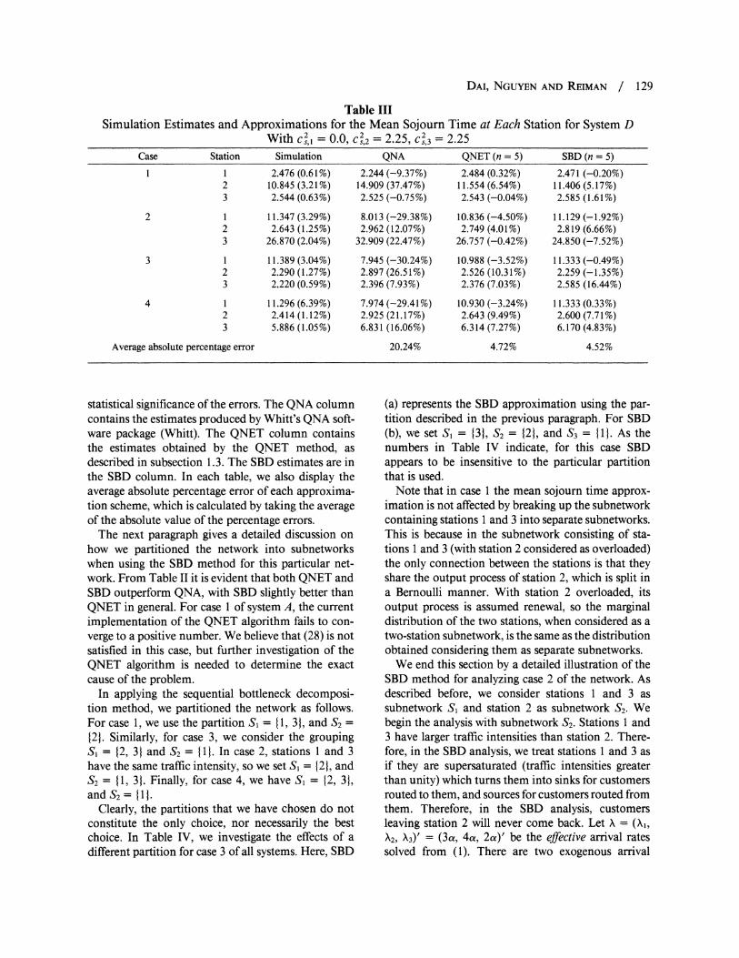
Clearly, the partitions that we have chosen do not constitute the only choice, nor necessarily the best choice. In Table IV, we investigate the effects of a different partition for case 3 of all systems. Here, SBD

(a) represents the SBD approximation using the partition described in the previous paragraph. For SBD (b), we set SI = 131, S2 = 121, and S3 = III. As the numbers in Table IV indicate, for this case SBD appears to be insensitive to the particular partition that is used.

Note that in case 1 the mean sojourn time approximation is not affected by breaking up the subnetwork containing stations 1 and 3 into separate subnetworks. This is because in the subnetwork consisting of stations 1 and 3 (with station 2 considered as overloaded) the only connection between the stations is that they share the output process of station 2, which is split in a Bernoulli manner. With station 2 overloaded, its output process is assumed renewal, so the marginal distribution of the two stations, when considered as a two-station subnetwork, is the same as the distribution obtained considering them as separate subnetworks.

We end this section by a detailed illustration of the SBD method for analyzing case 2 of the network. As described before, we consider stations 1 and 3 as subnetwork SI and station 2 as subnetwork S2. We begin the analysis with subnetwork S2. Stations 1 and 3 have larger trafflc intensities than station 2. There- fore, in the SBD analysis, we treat stations 1 and 3 as if they are supersaturated (traffic intensities greater than unity) which turns them into sinks for customers routed to them, and sources for customers routed from them. Therefore, in the SBD analysis, customers leaving station 2 will never come back. Let X = (X1, X2, X3)' = (3a, 4a, 2a)' be the effective arrival rates solved from (1). There are two exogenous arrival

Table III Simulation Estimates and Approximations for the Mean Sojourn Time at Each Station for System D

Withcs,1 =O.O,c,2=2.25,cS,3=2.25

Case Station Simulation QNA QNET (n = 5) SBD (n = 5)

I 1 2.476 (0.61%) 2.244 (-9.37%) 2.484 (0.32%) 2.471 (-0.20%) 2 10.845 (3.21%) 14.909 (37.47%) 11.554 (6.54%) 11.406 (5.17%) 3 2.544 (0.63%) 2.525 (-0.75%) 2.543 (-0.04%) 2.585 (1.61%)

2 1 11.347 (3.29%) 8.013 (-29.38%) 10.836 (-4.50%) 11.129 (-1.92%) 2 2.643 (1.25%) 2.962 (12.07%) 2.749 (4.01%) 2.819 (6.66%) 3 26.870 (2.04%) 32.909 (22.47%) 26.757 (-0.42%) 24.850 (-7.52%)

3 1 11.389 (3.04%) 7.945 (-30.24%) 10.988 (-3.52%) 11.333 (-0.49%) 2 2.290 (1.27%) 2.897 (26.51%) 2.526 (10.31%) 2.259 (-1.35%) 3 2.220 (0.59%) 2.396 (7.93%) 2.376 (7.03%) 2.585 (16.44%)

4 1 11.296 (6.39%) 7.974 (-29.41%) 10.930 (-3.24%) 11.333 (0.33%) 2 2.414 (1.12%) 2.925 (21.17%) 2.643 (9.49%) 2.600 (7.71%) 3 5.886 (1.05%) 6.831 (16.06%) 6.314 (7.27%) 6.170 (4.83%)



processes to station 2. One is a renewal arrival process ?I = {7R1(t), t > 01 from station 1, whose interarrival times have mean 1/X1 and squared coefficient of variation C2 1. The other is a "thinned" renewal process 172 = {n2(t), t > 01 from station 3. The incoming customers form a renewal counting process with interarrival times having mean 1 /X3 and squared coefficient of variation c2,3. An incoming customer from station 3 "flips" a fair coin, and goes to station 2 if the customer gets a head. It is easy to check that E[i7(t)] Xt and Var[nj(t)] X1c\2,It. Similarly we have E[72(t)] - (X3/2)t and Var[i2(t)] - [(X3/2) (1 + c2,3)/2]t. The superposition of these two arrival processes is the exogenous arrival processes to station 2, which has asymptotic rate XA + X3/2 = X2 and asymptotic variance X,1 + (X3/2)(1 + cs,3)/2.

Therefore,

W;2SBD

-T2(e) 2(C2+yACs,1+j2 ( C2))

-2 3 (Cs,2 + - Cs, I + 4 2 ) 32- 1/232 2 1(1_Ci\

3 27 C2 32+ ~ ~ s\ ,3

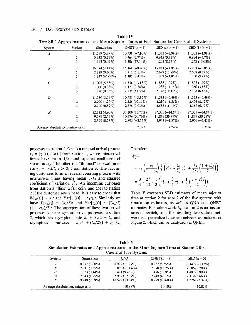
Table V compares SBD estimates of mean sojourn time at station 2 for case 2 of the five systems with simulation estimates, as well as QNA and QNET estimates. For subnetwork S1, station 2 is an instantaneous switch, and the resulting two-station network is a generalized Jackson network as pictured in Figure 2, which can be analyzed via QNET.

Table IV Two SBD Approximations of the Mean Sojourn Times at Each Station for Case 3 of all Systems

System Station Simulation QNET (n = 5) SBD (a) (n = 5) SBD (b) (n = 5)

A 1 11.559 (5.37%) 10.738 (-7.10%) 11.333 (-1.96%) 11.333 (-1.96%) 2 0.938 (0.21%) 0.964 (2.77%) 0.945 (0.75%) 0.894 (-4.7%) 3 1.113 (0.09%) 1.306 (17.34%) 1.205 (8.27%) 1.258 (13.03%)

B 1 16.484 (4.13%) 16.369 (-0.70%) 15.833 (-3.95%) 15.833 (-3.95%) 2 2.389 (0.50%) 2.512 (5.15%) 2.697 (12.89%) 2.608 (9.17%) 3 1.347 (67.04%) 1.393 (3.41%) 1.307 (-2.97%) 1.400 (3.93%)

C 1 11.705 (5.65%) 11.336 (-3.15%) 11.833 (1.09%) 11.833 (1.09%) 2 1.300 (0.38%) 1.422 (9.38%) 1.285 (-1.15%) 1.350 (3.85%) 3 1.976 (0.86%) 2.135 (8.05%) 2.176 (10.12%) 2.108 (6.68%)

D 1 11.389 (3.04%) 10.988 (-3.52%) 11.333 (-0.49%) 11.333 (-0.49%) 2 2.290 (1.27%) 2.526 (10.31%) 2.259 (-1.35%) 2.476 (8.12%) 3 2.220 (0.59%) 2.376 (7.03%) 2.585 (16.44%) 2.357 (6.17%)

E 1 32.132 (4.80%) 37.200 (15.77%) 27.333 (-14.94%) 27.333 (-14.94%) 2 9.089 (2.57%) 10.976 (20.76%) 11.849 (30.37%) 11.837 (30.23%) 3 2.999 (0.73%) 2.893 (-3.55%) 2.943 (-1.87%) 2.956 (-1.43%)


Table V Simulation Estimates and Approximations for the Mean Sojourn Time at Station 2 for

Case 2 of Five Systems System Simulation QNA QNET (n = 5) SBD (n = 5)

A 0.877 (0.00%) 0.982 (11.97%) 0.952 (8.55%) 0.847 (-3.42%) B 2.011 (0.65%) 1.869 (-7.06%) 2.378 (18.25%) 2.186 (8.70%) C 1.353 (0.44%) 1.481 (9.46%) 1.476 (9.09%) 1.407 (3.99%) D 2.643 (1.25%) 2.962 (12.07%) 2.749 (4.01%) 2.819 (6.66%) E 9.249 (2.39%) 10.529 (13.84%) 10.229 (10.60%) 11.776 (27.32%)



4

4

Figure 2. The two-station subnetwork SI.

3.2. A Five-Station Network Pictured in Figure 3 is a five-station generalized Jackson network. The exogenous arrival process to station 1 is Poisson with rate a = 1.0. We assume that service times at stations 2-5 have the same distribution. We further assume that the SCV of the service time at station 1 is the same as that at stations 2-5, and use c2 to denote the common SCV of the service times, i.e., c2 = c2i for i = 1,..., 5. We consider two versions of the network, labeled as systems A and B. In system A, all the service times are deterministic, which implies that c2 = 0. In system B, we allow more variability of the service times by taking c2 = 4. In each system, we again consider four different cases, whose parameters are given in Table VI. Note that by symmetry among stations 2 to 5 we have T3 = T4 =

T5 = T2, and consequently, P3 = P4 = P5 = P2. Thus, in the SBD analysis, stations 2 to 5 are always grouped as one subnetwork, and station 1 itself forms the other subnetwork. The simulation estimates and approximations for the total mean sojourn times for systems A and B are given in Table VII. The accuracy of QNET and SBD approximations are both impressive in this case, whereas the QNA approximations are not as accurate.

Table VI Mean Service Times of Four Cases of the

Five-Station Network Case TI T2 PI P2

1 0.400 1.2 0.80 0.60 2 0.300 1.6 0.60 0.80 3 0.400 1.5 0.80 0.75 4 0.375 1.6 0.75 0.80

3.3. Nine Stations in Series

Consider a generalized Jackson network consisting of nine single-server stations in series. Customers arrive at the first station according to a renewal process with interarrival times having a general distribution with mean 1 and squared coefficient of variation cc2,. The service-time distribution at station i is exponential (C2 = 1) with mean pi, where pi < 1. The traffic intensity at station i is pi = 0.6 for 1 < i < 8 and pq = 0.9. This network was chosen by Suresh and Whitt (1990b) to demonstrate the so called heavy- traffic bottleneck phenomenon: If the traffic intensity of one station is allowed to approach 1, then the waiting-time distribution at this bottleneck station is asymptotically the same as if the immediate arrival process (i.e., the departure process from the previous station) were replaced by the external arrival process to the first station. They showed that conventional parametric decomposition methods such as QNA fail to catch this heavy-traffic bottleneck phenomenon. They considered two cases for the interarrival times: high variability and low variability. The distribution for high variability is the hyperexponential (H2)

PoissonlX~

0.25 Ai

Poisson ~~ Fiur 3. A 0ie-25 io netork


distribution with balanced means and c2,1 = 8. The distribution for low variability is deterministic (D) with c,I = 0.

Tables VIII and IX give different estimates of the expected time at each station, as well as the total waiting time in the system. The simulation estimates

were taken from Suresh and Whitt (1 990a), and their simulation results show that customers will experience a long delay in queue 9 in both cases. When we apply the sequential bottleneck decomposition method as described in Section 2 to this network, there is a natural partition: SI = {1, 2, 3, 4, 5, 6, 7, 81 and

Table VII Simulation Estimates and Approximations for the Total Mean Sojourn Time of the Five-Station Network

System/Case Simulation QNA QNET (n = 5) SBD (n = 5)

A 1 6.725 (0.68%) 6.135 (-8.77%) 6.770 (0.67%) 6.950 (3.35%) 2 11.096 (5.59%) 9.959 (-10.25%) 10.998 (-0.88%) 11.345 (2.24%) 3 9.944 (0.68%) 8.911 (-10.39%) 9.842 (-1.03%) 9.576 (-3.70%) 4 11.567 (0.63%) 10.342 (-10.59%) 11.618 (0.44%) 11.998 (3.73%)

B 1 19.214 (0.64%) 21.512 (11.96%) 19.800 (3.05%) 19.150 (-0.33%) 2 35.948 (0.66%) 40.081 (11.50%) 34.832 (-3.10%) 35.648 (-0.83%) 3 33.676 (0.68%) 37.155 (10.33%) 34.416 (2.20%) 35.276 (4.75%) 4 40.704 (1.42%) 44.876 (10.25%) 39.338 (-3.36%) 39.803 (-2.21%)


Table VIII Simulation Estimates and Approximations of the Mean Steady-State Waiting Time at Each Station for

Nine Stations in Series With cla, = 0

Station Number Simulation QNA QNET (n = 4) SBD (n = 4)

1 0.290 (2.41%) 0.45 (55.17%) 0.45 (55.17%) 0.45 (55.17%) 2 0.491 (1.43%) 0.61 (24.24%) 0.66 (34.88%) 0.66 (35.01%) 3 0.607 (1.32%) 0.72 (18.62%) 0.74 (22.14%) 0.74 (22.29%) 4 0.666 (1.20%) 0.78 (17.12%) 0.79 (18.39%) 0.79 (18.58%) 5 0.706 (1.42%) 0.83 (17.56%) 0.82 (15.77%) 0.82 (16.00%) 6 0.731 (1.78%) 0.85 (16.28%) 0.84 (14.38%) 0.84 (14.63%) 7 0.748 (1.34%) 0.87 (16.31%) 0.85 (13.49%) 0.85 (13.76%) 8 0.775 (1.68%) 0.88 (13.55%) 0.86 (10.68%) 0.86 (10.91%) 9 5.031 (4.31%) 7.99 (58.82%) 6.97 (38.49%) 4.05 (-19.50%)

Total time in waiting 10.05 13.97 (39.00%) 13.01 (29.45%) 10.06 (0.09%)


Table IX Simulation Estimates and Approximations of the Mean Steady-State Waiting Time at Each Station

for Nine Stations in Series With c2, = 8 Station Number Simulation QNA QNET (n = 4) SBD (n = 4)

1 3.284 (3.50%) 4.05 (23.33%) 4.05 (23.33%) 4.05 (23.33%) 2 2.321 (4.18%) 2.92 (25.81%) 1.81 (-21.84%) 1.82 (-21.59%) 3 1.914 (3.40%) 2.19 (14.42%) 1.47 (-23.35%) 1.49 (-22.15%) 4 1.719 (4.07%) 1.73 (0.64%) 1.16 (-32.50%) 1.19 (-30.77%) 5 1.598 (3.69%) 1.43 (-10.51%) 1.07 (-32.90%) 1.10 (-31.16%) 6 1.478 (4.13%) 1.24 (-16.10%) 1.03 (-30.55%) 1.06 (-28.28%) 7 1.423 (3.23%) 1.12 (-21.29%) 1.00 (-29.71%) 1.03 (-27.62%) 8 1.413 (4.67%) 1.04 (-26.40%) 0.98 (-30.40%) 1.01 (-28.52%) 9 30.116 (16.84%) 8.90 (-70.45%) 6.04 (-79.95%) 36.45 (21.03%)

Total time in waiting 45.27 24.60 (-45.66%) 18.60 (-58.91%) 49.80 (10.01%)



S2 = {91. With this partition, station 9 is analyzed in isolation with stations 1-8 treated as instantaneous switches. Therefore, SBD analyzes station 9 as if it were a GIMII station with the same renewal arrival process as station 1. Hence, the average waiting time WgBD at station 9 is approximately given by

( 9p cq WgVBD~ - \p-p(I _ p1)

QNET is applied to S2 to obtain the SBD estimates of mean waiting times for stations 1-8. Note that, in both cases, the SBD estimates of total waiting time are very close to the simulation results. However, one can see from Tables VIII and IX that QNET, like QNA, fails to catch the heavy-traffic bottleneck phenomenon at station 9. Incidentally, the QNET estimates and SBD estimates of the mean waiting times at the first eight stations should be exactly the same. The small discrepancy is caused by the QNET algorithm when we fix (in both cases) n = 4 with dimension J= 8 and J= 9.

3.4. Ten Stations in Series

When there is high variability in an external arrival process, as in the second case of subsection 3.3 with C= 8.0, Suresh and Whitt (1990b) considered con- trolling the variability by filtering the arrival process through a low-variability station (i.e., by inserting a low variability station at the head of the network). In this section, we use their experiment to test our SBD method. The network model (system A) considered in this section is a modification of the network model from subsection 3.3, in which an extra station with deterministic service times is inserted before the same nine exponential stations. Hence, we have c2, = 0.

The remaining 9 stations do not change; they get relabeled so that now Pio = 0.9 and pi = 0.6 for 2 < i < 9. As before, c2, = 1 for 2 < i < 10. We consider two different traffic intensities for the first station, pI = 0.6 and 0.9. If pI = 0, we get back the nine stations in series considered in the previous section.

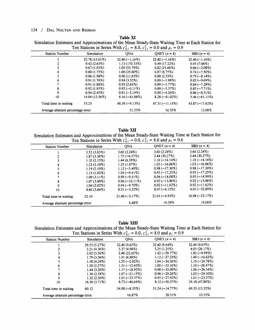
Tables X-XI give simulation estimates and different approximation estimates of the mean steady-state waiting times at each station for different traffic intensities at station 1. When p, = 0.6, station 10 is still the unique bottleneck station. Table X shows that SBD again predicts the bottleneck phenomenon at station 10 quite well. However, as shown in Table XI, SBD performs poorly when stations 1 and 10 are both bottleneck stations. One possible explanation of this is that SBD assumes that station 1 feeds immediately into station 10. Hence, c ljo is taken to be zero when in fact, due to intervening stations, it is not. The intervening stations are taken into account in both QNA and QNET. Tables XII-XIII report results for the dual examples (system B) in which the external arrival process is deterministic (c2 l = 0) and the first station has hyperexponential service times with cS, =

8.0. From Table XII we see that both QNET and QNA approximations perform very well in this case. The poor performance of SBD relative to QNA and QNET here has the same explanation as in the case of Table XI. SBD acts as if the input to the network (c,= 0) is fed directly into station 10. For the case Pi = 0.9, we see from Table XIII that high variability in the service times can also cause a much greater waiting time in a subsequent bottleneck station.

3.5. A Ten-Station Network With Feedback

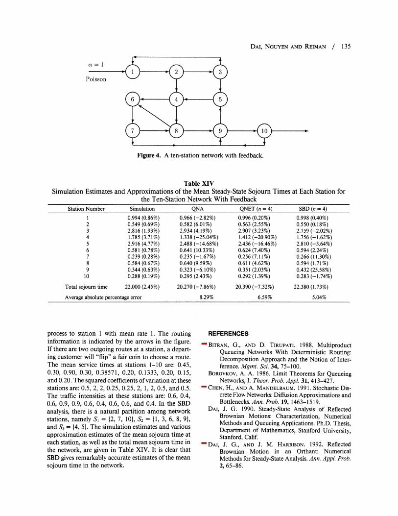
A ten-station generalized Jackson network is pictured in Figure 4. There is an exogenous Poisson arrival

Table X Simulation Estimates and Approximations of the Mean Steady-State Waiting Times at Each Station for

the Ten Stations in Series With c, I = 8.0, c ,l = 0.0 and Pi = 0.6


1 2.44 (3.69%) 3.60 (47.48%) 3.60 (47.48%) 3.60 (47.48%) 2 1.80 (3.90%) 2.75 (53.12%) 0.79 (-56.01%) 0.80 (-55.46%) 3 2.01 (4.38%) 2.09 (4.08%) 1.32 (-34.26%) 1.34 (-33.27%) 4 1.81 (3.32%) 1.66 (-8.24%) 1.25 (-30.90%) 1.27 (-29.80%) 5 1.66 (4.15%) 1.39 (-16.42%) 1.13 (-32.05%) 1.15 (-30.85%) 6 1.56 (3.65%) 1.21 (-22.54%) 1.06 (-32.14%) 1.08 (-30.86%) 7 1.45 (3.80%) 1.10 (-24.09%) 1.01 (-30.30%) 1.04 (-28.23%) 8 1.41 (3.27%) -1.03 (-26.69%) 0.98 (-30.25%) 1.01 (-28.11%) 9 1.40 (4.72%) 0.98 (-29.90%) 0.96 (-31.33%) 0.99 (-29.18%)

10 29.97 (16.90%) 8.57 (-71.40%) 5.14 (-82.85%) 36.45 (21.62%)



134 / DAI. NGUYEN AND REIMAN

Table XI Simulation Estimates and Approximations of the Mean Steady-State Waiting Time at Each Station for

Ten Stations in Series With cd,i = 8.0, c2, = 0.0 and P1 = 0.9 Station Number Simulation QNA QNET (n = 4) SBD (n = 4)

1 32.78 (15.61%) 32.40 (-1.16%) 32.40 (-1.16%) 32.40 (-1.16%) 2 0.42 (2.63%) 1.13 (170.33%) 0.49 (17.22%) 0.45 (7.66%) 3 0.67 (1.93%) 1.05 (55.79%) 0.82 (21.66%) 0.66 (-2.08%) 4 0.80 (1.75%) 1.00 (25.00%) 0.87 (8.75%) 0.74 (-7.50%) 5 0.86 (1.98%) 0.96 (11.63%) 0.88 (2.33%) 0.79 (-8.14%) 6 0.91 (1.76%) 0.94 (3.52%) 0.89 (-1.98%) 0.82 (-9.69%) 7 0.91 (1.88%) 0.93 (2.65%) 0.89 (-1.77%) 0.84 (-7.28%) 8 0.92 (1.95%) 0.92 (-0.11%) 0.89 (-3.37%) 0.85 (-7.71%) 9 0.94 (2.45%) 0.91 (-3.19%) 0.90 (-4.26%) 0.86 (-8.51%)

10 14.04 (13.56%) 8.16 (-41.88%) 8.28 (-41.02%) 5.46 (-61.11%)

Total time in waiting 53.25 48.39 (-9.13%) 47.31 (-11.15%) 43.87 (-17.62%)


Table XII Simulation Estimates and Approximations of the Mean Steady-State Waiting Time at Each Station for

Ten Stations in Series With c2 1 = 0.0, c2l = 8.0 and P1 = 0.6


1 3.52 (3.83%) 3.60 (2.24%) 3.60 (2.24%) 3.60 (2.24%) 2 1.87 (3.36%) 1.75 (-6.57%) 2.44 (30.27%) 2.44 (30.27%) 3 1.35 (2.15%) 1.44 (6.59%) 1.16 (-14.14%) 1.16 (-14.14%) 4 1.23 (3.10%) 1.25 (1.87%) 1.03 (-16.06%) 1.03 (-16.06%) 5 1.19 (2.19%) 1.12 (-5.49%) 0.98 (-17.30%) 0.98 (-17.30%) 6 1.15 (1.83%) 1.04 (-9.41%) 0.95 (-17.25%) 0.95 (-17.25%) 7 1.09 (3.11%) 0.99 (-9.51%) 0.94 (-14.08%) 0.93 (-14.99%) 8 1.07 (3.00%) 0.96 (-10.11%) 0.92 (-13.86%) 0.92 (-13.86%) 9 1.04 (2.02%) 0.94 (-9.70%) 0.92 (-11.62%) 0.92 (-11.62%)

10 8.60 (3.66%) 8.31 (-3.33%) 8.07 (-6.12%) 4.05 (-52.89%)

Total time in waiting 22.10 21.40 (-3.17%) 21.01 (-4.93%) 16.98 (-23.17%)


Table XIII Simulation Estimates and Approximations of the Mean Steady-State Waiting Time at Each Station for

Ten Stations in Series With c2,1 = 0.0, c2 l = 8.0 and P1 = 0.9 ,~~~~~~~~~~~~ .,c, 8. an i .

Station Number Simulation QNA QNET (n = 4) SBD (n =4)

1 29.55 (5.27%) 32.40 (9.65%) 32.40 (9.64%) 32.40 (9.65%) 2 3.21 (4.36%) 3.37 (4.98%) 3.25 (1.25%) 4.05 (26.17%) 3 2.02 (3.56%) 2.48 (22.65%) 1.42 (-29.77%) 1.82 (-9.99%) 4 1.79 (3.36%) 1.91 (6.88%) 1.12 (-37.33%) 1.49 (-16.62%) 5 1.58 (4.24%) 1.55 (-2.02%) 1.04 (-34.26%) 1.19 (-24.78%) 6 1.50 (2.27%) 1.31 (-12.43%) 1.00 (-33.16%) 1.10 (-26.47%) 7 1.44 (3.26%) 1.17 (-18.92%) 0.98 (-32.09%) 1.06 (-26.54%) 8 1.36 (2.58%) 1.07 (-21.15%) 0.96 (-29.26%) 1.03 (-24.10%) 9 1.32 (2.50%) 1.01 (-23.37%) 0.95 (-27.92%) 1.01 (-23.37%)

10 16.36 (5.71%) 8.73 (-46.64%) 8.12 (-50.37%) 24.18 (47.80%)




process to station 1 with mean rate 1. The routing information is indicated by the arrows in the figure. If there are two outgoing routes at a station, a departing customer will "flip" a fair coin to choose a route. The mean service times at stations 1-10 are: 0.45, 0.30, 0.90, 0.30, 0.38571, 0.20, 0.1333, 0.20, 0.15, and 0.20. The squared coefficients of variation at these stations are: 0.5, 2, 2, 0.25, 0.25, 2, 1, 2, 0.5, and 0.5. The traffic intensities at these stations are: 0.6, 0.4, 0.6, 0.9, 0.9, 0.6, 0.4, 0.6, 0.6, and 0.4. In the SBD analysis, there is a natural partition among network stations, namely SI = 12, 7, 0l, S2 = {1, 3, 6, 8, 9}, and S3 = 14, 5}. The simulation estimates and various approximation estimates of the mean sojourn time at each station, as well as the total mean sojourn time in the network, are given in Table XIV. It is clear that SBD gives remarkably accurate estimates of the mean sojourn time in the network.

REFERENCES

BITRAN, G., AND D. TIRUPATI. 1988. Multiproduct Queueing Networks With Deterministic Routing: Decomposition Approach and the Notion of Inter- ference. Mgmt. Sci. 34, 75-100.

BOROVKov, A. A. 1986. Limit Theorems for Queueing Networks, I. Theor. Prob. Appl. 31, 413-427.

CHEN, H., AND A. MANDELBAUM. 1991. Stochastic Dis- crete Flow Networks: Diffusion Approximations and Bottlenecks. Ann. Prob. 19, 1463-1519.

DAI, J. G. 1990. Steady-State Analysis of Reflected Brownian Motions: Characterization, Numerical Methods and Queueing Applications. Ph.D. Thesis, Department of Mathematics, Stanford University, Stanford, Calif.

DAI, J. G., AND J. M. HARRISON. 1992. Reflected Brownian Motion in an Orthant: Numerical Methods for Steady-State Analysis. Ann. Appl. Prob. 2, 65-86.

Figure 4. A ten-station network with feedback.

Table XIV Simulation Estimates and Approximations of the Mean Steady-State Sojourn Times at Each Station for

the Ten-Station Network With Feedback Station Number Simulation QNA QNET (n = 4) SBD (n = 4)

1 0.994 (0.86%) 0.966 (-2.82%) 0.996 (0.20%) 0.998 (0.40%) 2 0.549 (0.69%) 0.582 (6.01%) 0.563 (2.55%) 0.550 (0.18%) 3 2.816 (1.93%) 2.934 (4.19%) 2.907 (3.23%) 2.759 (-2.02%) 4 1.785 (3.71%) 1.338 (-25.04%) 1.412 (-20.90%) 1.756 (-1.62%) 5 2.916 (4.77%) 2.488 (-14.68%) 2.436 (-16.46%) 2.810 (-3.64%) 6 0.581 (0.78%) 0.641 (10.33%) 0.624 (7.40%) 0.594 (2.24%) 7 0.239 (0.28%) 0.235 (-1.67%) 0.256 (7.11%) 0.266 (11.30%) 8 0.584 (0.67%) 0.640 (9.59%) 0.611 (4.62%) 0.594 (1.71%) 9 0.344 (0.63%) 0.323 (-6.10%) 0.351 (2.03%) 0.432 (25.58%)

10 0.288 (0.19%) 0.295 (2.43%) 0.292 (1.39%) 0.283 (-1.74%)

Total sojourn time 22.000 (2.45%) 20.270 (-7.86%) 20.390 (-7.32%) 22.380 (1.73%)


136 / DAI. NGUYEN AND REIMAN

HARRISON, J. M., AND R. WILLIAMS. 1987. Brownian Models of Open Queueing Networks With Homo- geneous Customer Populations. Stochastics 22, 77-115.

HARRISON, J. M. AND V. NGUYEN. 1990. The QNET Method for Two-Moment Analysis of Open Queueing Networks. Queue. Syst. 6, 1-32.

JACKSON, J. R. 1957. Networks of Waiting Lines. Opns. Res. 5, 518-521.

JOHNSON, D. P. 1983. Diffusion Approximation for Opti- mal Filtering of Jump Processes and for Queueing Networks. Ph.D. Thesis, University of Wisconsin, Madison.

KRAEMER, W., AND M. LANGENBACH-BELZ. 1976. Approximate Formulae for the Delay in the Queueing System GI/G/1. Eighth Int. Teletraffic Congress, 235.1-235.8.

KUEHN, P. J. 1979. Approximate Analysis of General Queueing Networks by Decomposition. IEEE Trans. Commun. 27, 113-126.

REIMAN, M. I. 1984. Open Queueing Networks in Heavy Trafflc. Math. Opns. Res. 9, 441-458.

REIMAN, M. 1. 1990. Asymptotically Exact Decomposi- tion Approximations for Open Queueing Networks. OR Letts. 9, 363-370.

SURESH, S., AND W. WHITT. 1 990a. Arranging Queues in Series: A Simulation Experiment. Mgmt. Sci. 36, 1080-1091.

SURESH, S., AND W. WHITT. 1990b. The Heavy-Traffic Bottleneck Phenomenon in Open Queueing Net- works. OR Letts. 9, 355-362.

WHITT, W. 1983. The Queueing Network Analyzer. Bell Sys. Tech. J. 62, 2779-2815.

sequential bottleneck decomposition: an … · 2008-12-14 · sequential bottleneck decomposition:...

Documents